modeling generalized cylinders using direction map representation
TRANSCRIPT

Modeling generalized cylinders using direction map representation
Joo-Haeng Lee*
Intelligent Robot Lab, ETRI, 161 Gajeong-dong, Yuseong-gu, Daejeon 305-350, South Korea
Accepted 20 September 2004
Abstract
For generalized cylinders (GC) defined by contours of discrete curves, we propose two algorithms to generate GC surfaces (1) in polygonal
meshes and (2) in developable surface patches of the cylindrical type. To solve the contour blending problem of generalized cylinder, the
presented algorithms have adopted the algorithms and properties of linear interpolation by direction map (LIDM) that interpolate geometric
shapes based on direction map merging and group scaling operations. Moreover, we propose an algorithm to develop generated developable
surface patches on a plane. Proposed algorithms are fast to compute and easy to implement.
q 2005 Elsevier Ltd. All rights reserved.
Keywords: Generalized cylinder; Direction map representation; Developable surface
1. Introduction
Generalized cylinder (GC) is a well-known modeling
technique to design tube-like shapes whose surfaces are
constructed over skeletal frames composed of a finite
sequence of contours (2D cross-sectional curves) that are
systematically arranged on a 3D spine curve. (Initial
contours are referred to as control contours) Generally, the
spine curve determines the overall shape, and contours
expresses detailed features on the surface.
By interpolating (or blending) the given contours, we can
generate a one-parameter family of contours which
conceptually sweeps along the spine curve while changing
its orientation and shape. Using this general sweep analogy,
we can represent a GC as a tensor product surface with two
parameters representing the spine and the contour
directions, respectively. After generating the surface from
the initial design, we can interact with the skeletal curves
or the surface itself to change the shape characteristics. With
these simple building blocks and mechanisms coupled with
other geometric modeling techniques, we can design various
kinds of artificial shapes (i.e. pipes, vessels, and tires)
and natural shapes (i.e. human bodies, flowers,
0010-4485//$ - see front matter q 2005 Elsevier Ltd. All rights reserved.
doi:10.1016/j.cad.2004.09.012
* Tel.: C82 42 860 1338; fax: C82 42 860 6790.
E-mail address: [email protected].
and seashells) as GC models for CAD and computer
graphics applications.
Previous researches have focused on various GC topics
such as surface representations, deformation and interaction
techniques, and orientation arrangements. Note that, to be
integrated with general purpose geometric modeling tools, it
is a common practice to generate surface models directly
from the intrinsic definition of GC: i.e. a spine curve and a
sequence of contour curves. Hence, there are abundant
research works presenting how to represent GC surfaces as a
polyhedral mesh [1], Bezier [6], B-spline [14], or NURBS
surfaces [4] from the given skeletal frames. Some
representation methods focus on the direct ray-casting [14]
without converting into specific representations. We can find
researches presenting special representations suitable for
interactive deformation [4,6]. Contour arrangement with a
smooth orientation change is simply achieved by
embedding a contour on the normal plane [3] of the Frenet
frame [4,6,14]. For better results, rotation minimizing frame
can optimize distortion [7]. As a more sophisticated topic,
Gansca et al. [5] deals with the problem of self-intersection
avoidance in the generation of GC surfaces.
Another important GC topic is contour blending, which
is required to generate a one-parameter family of contours
continuously. One of the fundamental steps for contour
blending is to set up correspondences between features of
adjacent control contours. However, in most of previous
Computer-Aided Design 37 (2005) 837–846
www.elsevier.com/locate/cad

J.-H. Lee / Computer-Aided Design 37 (2005) 837–846838
approaches, these correspondences are assumed to be
described manually or implicitly. For example, although
very complicated contours were illustrated in B-Spline
surface approach of de Voogt et al. [14], no explicit step is
specified for setting correspondences between every pair of
control points from adjacent contours. This is partly because
every contour has the same number of control points, which
may lead to trivial correspondences in a certain case.
However, this is not the case of real-world examples where
correspondences are rather complicated to be described
manually or assumed implicitly.
This correspondence problem is also fundamental in
morphing. (Note that morphing is generally composed of
two steps: (1) correspondences and (2) path interpolation.)
When key-frame shapes are not so complex, existing
geometric morphing techniques work relatively fine.
However, we can hardly expect full automation: for better
result, a human intervention is inevitable. For example,
when we want to generate a sequence of in-betweens
interpolating given key-frames representing different pos-
tures of a dancer [12], we cannot specify a semantic
constraint such as ‘an arm should not be morphed to a leg’
based on geometric intelligence of the previous algorithms.
In addition, most of morphing techniques cannot express
interpolating path in the form of parametric curves. If we
consider contours as key-frames, the parametric represen-
tation of interpolating path is critical to generate the surfaces
of a GC.
In this paper, we suggest to adopt a geometric morphing
technique referred to as linear interpolation by direction
map (LIDM) proposed by Lee et al. [9] to solve both
correspondence and parametric interpolation problems in
contour blending. LIDM is closely related to previous
morphing technique referred to as linear interpolation by
Minkowski sum (LIMS) [8,11], but more generalized and
computationally efficient.
As a main contribution, we present methods to construct
GC surface with (1) polygonal mesh and (2) developable
surface patches of the cylindrical type using the geometric
properties of LIDM. The overall computation of proposed
methods is fast enough to be applied in interactive
geometric design applications. In addition, we also propose
an algorithm to make plane-development figures for a GC
whose surface is represented by developable surface patches
of the cylindrical type.
The remainder of this paper is organized as follows. In
Section 2, we describe a typical representation of parametric
GC surface and explain why contour blending problem
matters in GC design. In Section 3, we propose to adopt
LIDM method as a contour blending method in GC design.
In Section 4, we describe how to build a polygonal mesh of
GC whose control contours are blended by LIDM. In
Section 5, we describe how to represent the surface of a GC
as a set of developable surface of the cylindrical type. In
Section 6, we explain how to develop generated developable
surface patches on a plane, and demonstrate the example
results. In Section 7, we summarize this paper briefly.
2. Parametric representation of GC
Let each contour curve be placed on a contour plane. For
a spine curve parameterized as KðuÞ2R3, we can choose a
contour plane Nðu0Þ2R3 as the normal plane at K(u0),
which is intrinsically defined as a part of the Frenet frame
[3]. (As in Chang et al. [4], we can define the orientation
more generally—independently of differential
characteristics of the given spine curve.) In this case,
N(u0) is spanned by its normal and binormal vectors, nx(u)
and ny(u), and its local origin is placed at K(u0).
When a 2D contour curve �Cu0Z ðxu0
ðvÞ; yu0ðvÞÞ is
embedded in N(u0), it has the following parametric form
in 3D:
Cu0ðvÞ Z xu0
ðvÞ$nxðu0ÞCyu0ðvÞ$nyðu0Þ (1)
However, considering that every contour may have a
different shape at K(u), above parametric form should be
further generalized as follows:
CuðvÞ Z xuðvÞ$nxðuÞCyuðvÞ$nyðuÞ (2)
hCðu; vÞ (3)
Z xðu; vÞ$nxðuÞCyðu; vÞ$nyðuÞ: (4)
When we consider GC as a sweep surface of a moving
contour, the parametric form of GC surface S is generated
by sweeping Cu(v) along K(u) as follows:
Sðu; vÞ Z Cðu; vÞCKðuÞ
Z xuðvÞ$nxðuÞCyuðvÞ$nyðuÞCKðuÞ: (5)
In the above equation, we assume that a pair of
coordinate functions (xu(v),yu(v)) is defined at every point
K(u) of the spine curve; however, a human designer could
not specify infinite number of coordinate functions
manually at each value of u. This is the point where contour
blending problem arises: how do we smoothly interpolate a
finite set of control contours to generate a certain number of
in-between contours required to satisfy the given precision
criteria?
In this paper, to be more focused on the blending problem
itself, we can confine the bases of the contour plane to be
fixed over u. In this case, a GC surface has a simple
parametric form as follows:
Sðu; vÞ Z xuðvÞ$nx CyuðvÞ$ny CKðuÞ: (6)
This is the typical case when the spine curve is a straight
line segment. Specially, the developable surface examples
in Sections 5 and 6 are of this type.
J.-H. Lee / Computer-Aided Design 37 (2005) 837–846 839
3. Contour blending by LIDM
Recently, Lee et al. [9] proposed an efficient algorithm
referred to as linear interpolation by direction map (LIDM)
to interpolate two polygonal shapes. Moreover, a designer
can specify additional control shapes, which enables a
Bezier-curve or blossom-like control structure. The result of
LIDM is a sequence of interpolated polygons—a one-
parameter family of polygons. Specially, the automatic
correspondences work quite well for relatively simple
shapes rather than the complex ones required in character
animation applications. Note that GC does not require such
complex contours as in character animations. Hence, we
propose to adopt LIDM as a contour blending method in GC
design.
In LIDM, a polygon is represented by a circular list of
direction vectors, which is referred to as a direction map. A
direction vector is defined as a connecting vector of two
neighboring polygon vertices. A group of consecutive
direction vectors may represent a geometric feature such
as pocket, chamfer, and fillet. An important property of
LIDM is that the direction itself of any direction vector is
invariant through the interpolation process. Hence, (1) the
sequence of directions and (2) lengths of individual
direction vectors are key factors determining the actual
shape of a feature.
We can generate a new polygon by merging two
direction maps representing different shapes. This step is
analogous with blending features from different polygons.
When merging direction maps, we change neither the
direction nor the length of any direction vector; rather, the
sequence of direction vectors is newly generated after
merging with a certain geometric correspondence rule.
Among various feature correspondence strategies, convolu-
tion merging is closely related to Minkowski sum or
convolution operations, where vertex-wise feature corre-
spondences are set up by a certain geometric rule [9]. Note
that LIMS (linear interpolation by Minkowski sum [8,11]) is
a special case of LIDM. If we apply a different merging rule
such as convex-hull merging, the result of LIDM becomes
quite different from that of LIMS.
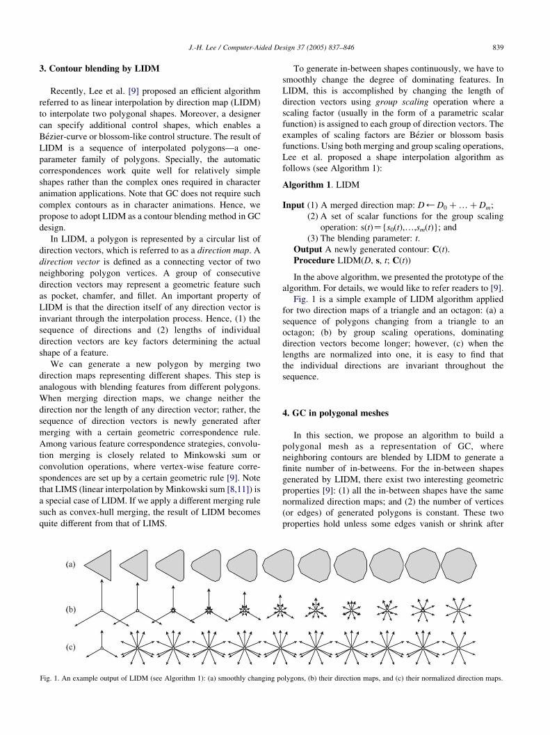
Fig. 1. An example output of LIDM (see Algorithm 1): (a) smoothly changing p
To generate in-between shapes continuously, we have to
smoothly change the degree of dominating features. In
LIDM, this is accomplished by changing the length of
direction vectors using group scaling operation where a
scaling factor (usually in the form of a parametric scalar
function) is assigned to each group of direction vectors. The
examples of scaling factors are Bezier or blossom basis
functions. Using both merging and group scaling operations,
Lee et al. proposed a shape interpolation algorithm as
follows (see Algorithm 1):
Algorithm 1. LIDM
Inp
olyg
ut (1) A merged direction map: D)D0 þ . þ Dm;
(2) A set of scalar functions for the group scalingoperation: s(t)Z{s0(t),.,sm(t)}; and
(3) The blending parameter: t.
Output A newly generated contour: C(t).
Procedure LIDM(D, s, t; C(t))
In the above algorithm, we presented the prototype of the
algorithm. For details, we would like to refer readers to [9].
Fig. 1 is a simple example of LIDM algorithm applied
for two direction maps of a triangle and an octagon: (a) a
sequence of polygons changing from a triangle to an
octagon; (b) by group scaling operations, dominating
direction vectors become longer; however, (c) when the
lengths are normalized into one, it is easy to find that
the individual directions are invariant throughout the
sequence.
4. GC in polygonal meshes
In this section, we propose an algorithm to build a
polygonal mesh as a representation of GC, where
neighboring contours are blended by LIDM to generate a
finite number of in-betweens. For the in-between shapes
generated by LIDM, there exist two interesting geometric
properties [9]: (1) all the in-between shapes have the same
normalized direction maps; and (2) the number of vertices
(or edges) of generated polygons is constant. These two
properties hold unless some edges vanish or shrink after
ons, (b) their direction maps, and (c) their normalized direction maps.

J.-H. Lee / Computer-Aided Design 37 (2005) 837–846840
trimming. (In the example of Fig. 1, the number of vertices
of every in-between polygon is constant as 11Z3C8.)
Based on these properties, it is straightforward to build
triangular (or quad) meshes by connecting corresponding
vertices from neighboring contours. See Algorithm 2
below.
Algorithm 2. LIDM-GC-Mesh
Fig
gen
Input (1) Two terminal contours and additional control
contours: CZ{C0,.,Cm};
(2) A set of scalar functions (i.e. Bernstein poly-
nomials): bZ{b0(t),.,bm(t)}; and
(3) The number of in-between contours to be generated:
n.
. 2. A
erate
Output A polygonal mesh interpolating given control
contours: M.
Procedure
1. D)D0C/CDm; /* to merge directions maps:
DiZDM(Ai) */
2. l)jDj; /* the number of dir. vectors in the merged
direction map */
3. Cprev)C(0)ZLIDM(D,b,0); /* to compute the
initial contour */
4. For iZ1 to (nC1)
5. ti)tZDt*i; /* DtZ1/(nC1) */
6. Ccurr)C(t)ZLIDM(D,b,ti); /* assuming
jDM(C(t))j is invariant. */
7. Mi):; /* At first the ith sub-mesh is empty. */
8. For jZ1 to l /* to construct a sub-mesh Mi
connecting Cprev and Ccurr */
9. mj)two triangle (or a quadrangle) constructed
using the corresponding four vertices: jth and
(jC1)th vertices of Cprev and Ccurr;
n example result of LIDM-GC-Mesh (see Algorithm 2): (a) control contours
d polygonal mesh, and (d) shaded result of (c).
10. Mi)Migmj; /* incremental addition of mesh
elements */
11. M)MgMi;
12. Cprev)Cnext; /* incremental addition of sub-
mesh */
(in pi
In Algorithm 2, each execution of LIDM at ti (see the
line 6) generates one intermediate contour C(ti). Note that,
however, direction map merging is computed just once
during the whole execution since the feature correspon-
dences are assumed to be static. (See the line 1 which is
outside the main loop starting at the line 4).
Each sub-mesh Mi is generated by connecting two
consecutive contours, Cprev and Ccurr. (See the lines from
8–10.) The edge connection rules are simple. For
example, to generate two triangles: (1) connect two
starting points, (2) two end points of corresponding edge,
and (3) choose one diagonal. The final mesh M is
generated by sequentially combining all the sub-meshes
Mi (See the line 11).
Fig. 2 illustrates the execution of LIDM-GC-Mesh
algorithm. Fig. 2(a) shows four control contours (in pink)
arranged on a spine curve: from the bottom, a cross, a
rectangle, a polygon of the circular shape, and a letter H. In
Fig. 2(b), gray contours are blended in-betweens
generated by LIDM. By connecting the result of Fig. 2(b),
LIDM-GC-Mesh can generate a mesh representing
the surface of a GC (See Fig. 2(c)). For display, we can
apply standard mesh shading to the generated mesh
(See Fig. 2(d)).
When correspondences should be made for direction
maps of trimmed contours, more sophisticated rules should
be applied to handle exceptions. We skip details here.
nk) arranged on a spine line, (b) blended contours (in gray), (c) the

J.-H. Lee / Computer-Aided Design 37 (2005) 837–846 841
For relatively simple non-convex contours, we can apply the
convex-hull merging rule to avoid trimming, and to make
the correspondences simpler.
5. GC in developable surface patches
In this section, we describe how to represent the surface
of a GC as a set of developable surface of the cylindrical
type. A developable surface is a special type of ruled
surface, where all the points from one ruling have the same
tangent plane [3]. Specially, a developable surface can be
unfolded (or developed) into a plane without stretching or
tearing. Hence, it has a wide-range of applications in
manufacturing based on sheet metal-like materials. The
recent works shows that a developable surface has a nice
structure of controllability [2] and a neat representation in
NURBS [10].
When every control contour has the same orientation (i.e.
not on the normal plane of Frenet frame but on the plane
parallel to a reference plane), corresponding edges of
blended contours are parallel to each other since they are
constructed by the same direction vector whose direction is
invariant throughout the interpolation process. Hence, each
direction vector di (moving along a certain directrix curve)
defines one developable surface patch Si of the cylindrical
type. It is a well-known fact that a ruling direction which is
fixed over a directrix defines a developable surface of the
cylindrical type [3].
Each developable surface patch Si is bounded by two
boundary curves: FiK1(u) and Fi(u). Let these curves be
profile curves. Each profile curve Fi(u) is identical to the
sweep trajectory of the ith vertex of the intermediate contour
C(u). In addition, based on the properties of merged direction
map and group scaling operation [9], every vertex of the
intermediate contour C(u) is defined by blending (mC1)
vertices {pi,0,.,pi,m}, each of which is chosen from one of
given control contours {C0,.,Cm}. In the above blending,
the weights are defined by the blending functions used in
group scaling operation.
For example, when applying Bernstein polynomials as
blending functions, a profile curve is represented as follows:
FiðuÞ ZXm
jZ0
Bmj ðuÞ$pi;j: (7)
According to the above equation, the relevant vertex pi,j
from the control contour Cj constitutes the control points of
the profile curve Fi(u). Actually, the type of boundary curve
(or surface) is defined by how we blend the given control
contours using a certain scaling factors such as blossom or
NURBS basis functions.
It is clear that profile curves satisfy the following
condition:
hFiðuÞKFiK1ðuÞ;dii Z 0: (8)
This leads to the following relation for every pair of
neighboring control points:
hpi;j KpiK1;j; dii Z 0: (9)
Hence, control points of FiK1(u) and Fi(u) are identical
except the direction (pi,jKpiK1,j)s0 is parallel to di.
Using this property, Algorithm 3 can find a set of control
points of each profile curve regardless of convexity of
control contours.
Algorithm 3. LIDM-GC-Dvlp
Input Two terminal contours and additional control
contours: CZ{C0,.,Cm};
Output Sets of control points defining boundary curves
of developable surface patches: PZ{P1,.,Pi} where
PiZ{pi,0,.,pi,m} and Pi defines a boundary curve Fi.
Procedure
1. D)D0C/CDm; /* merge directions maps: DiZDM(Ai) */
2. l)jDj; /* the number of direction vectors in D*/
3. for iZ1 to l /* for each profile curve Fl defined by a
direction vector di */
4. di) the ith direction vector of D;
5. Pi):;
6. for jZ0 to m /* find each set of control points Pi
defining Fi*/
7. d) find a direction vector of D that following
two conditions:
(1) the counter-clockwise nearest direction vector
from di in D (including di); and
(2) its group id is j; /* selecting a single vertex
from Cj */
8. Pi,j)the vertex of Cj corresponding to the end
point of d;
9. Pi)Pig{pi,j};/* finding each set of control
points */
10. P)Pg{pi};/* finding all the sets of control
points */
If we apply Bernstein polynomials of degree m as scaling
factors for the group scaling operation, each developable
surface can be represented as Bezier surface of degree (m, 1)
as follows
Siðu; vÞ Z ð1 KvÞFiK1ðuÞCvFiðuÞ (10)
Z ð1 KvÞXm
jZ0
Bmj ðuÞ$piK1;j Cv
Xm
jZ0
Bmj ðuÞ$pi;j
ZXm
jZ0
X1
kZ0
Bmj ðuÞB
1kðuÞ$piK1Ck;j; (11)
where i2{1,.,l}.
Fig. 3 shows an example result of where each patch is a
Bezier surface of degree (3, 1). In Fig. 3(a), four control

Fig. 3. An example result of LIDM-GC-Dvlp (see Algorithm 3): (a) control contours; (b) blended contours (in gray); (c) meshes (in gradient color) and a
developable surface patch (in cyan); (d) control points (connected by green lines) of boundary curves; (e) the control points of all boundary curves; and
(f) developable surface patches and their control points.
J.-H. Lee / Computer-Aided Design 37 (2005) 837–846842
contours—in this case, quadrangles of different sizes—are
placed on a straight line with the same orientation. In
Fig. 3(b), blended contours (in gray) are generated by
LIDM-GC-Mesh algorithm using Bernstein polynomials as
blending functions (i.e. scalar functions of group scaling
operation). In Fig. 3(c), when a mesh (in gradient color) is
displayed, we can easily observe an approximated devel-
opable surface patch (in cyan) bounded by two boundary
curves. (Note that, although LIDM-GC-Mesh is used in
Fig. 3(b) for the purpose of explanation, it has no
dependency on LIDM-GC-Dvlp.)
In Fig. 3(d), for each developable surface patch, we
can select a set of control points (connected by green line)
of each boundary curve among the vertices of control
contours using LIDM-GC-Dvlp algorithm. In Fig. 3(e),
after we find all the control points, we can evaluate the
boundary curves as Bezier curves. (Evaluated boundary
curves give an impression of the GC shape.) Otherwise, as
in Fig. 3(f), we can adopt existing shading algorithms for
Bezier surfaces.
Note that LIDM-GC-Dvlp is more powerful than
LIDM-GC-Mesh. If we want to generate in-between
contours using LIDM-GC-Dvlp, we can connect the points
from every boundary curves evaluated at the same value in
sequential order. For example, a contour at the spine
curve K(u) is defined by following vertices: {F1(u),F2
(u),.,Fl(u)}. However, it is not easy to generate a
parametric form of boundary curves using LIDM-GC-
Mesh since it is based on contour-wise evaluations.
6. Plane development of GC
In this section, we explain plane development algorithm
for the developable surface patches generated by LIDM-
GC-Dvlp. In addition, we provide examples experimented
with real paper patches.
In Fig. 4(a), a developable surface patch Si (the same one
introduced in Fig. 3(d)) is defined by the ruling parallel to
direction vector di along a certain directrix curve.
For plane development, we define a special directrix
curve Fdi ðtÞ for each developable surface patch Si that is
normal to di Such a directrix curve is referred to as
normal directrix, which is the trace of principal direction
along the maximum normal curvature. We can derive
control points pdi;j (connect in red lines in Fig. 4(a)) of

Fig. 4. Development of a developable surface patch on a plane: (a) finding the control points (connected in red line) of a normal directrix curve, (b) the normal
directrix and its control points on a plane normal to the direction vector di, and (c) developing on a plane whose coordinate axis are defined by the normal
directrix and direction vector.
J.-H. Lee / Computer-Aided Design 37 (2005) 837–846 843
Fdi ðtÞ as follows
di Z pi;j KpiK1;j; di s0 (12)
piK1;0 Z pdi;0; (13)
piK1;j Z pdi;j ChL
i;j$di; (14)
pi;j Z pdi;j ChU
i;j$di (15)
Z pdiC1;j ChL
iC1;j$diC1; (16)
where hL� and hU
� are scalar values. Based on the planarity
of pdi;j, the following property holds:
0 Z hðpdiK1;j Kpd
iK1;0Þ; dii (17)
Z hðpiK1;j KhLi;j$di KpiK1;0Þ;dii (18)
Using above property, we can sequentially derive the
following equations:
hLi;j Z
hðpiK1;j KpiK1;0Þ;dii
hdi; dii(19)
pdi;j Z piK1;j KhL
i;j$di (20)
hUi;j Z
hðpi;j Kpdi;jÞ; dii
hdi; dii(21)
Now, we can derive the profile curve as follows:
FiK1ðtÞ ZXm
jZ0
B3j ðtÞ$piK1;j (22)
ZXm
jZ0
B3j ðtÞ$ðp
di;j ChU
i;j$diÞ (23)
FiK1ðtÞ ZXm
jZ0
B3j ðtÞ$pd
i;j CXm
jZ0
B3j ðtÞ$hL
i;j
!$di
Z Fdi ðtÞCHL
i ðtÞ$di (24)
Similarly, we can derive the neighboring profile curve as
follows:
FiðtÞ Z Fdi ðtÞCHU
i ðtÞ$di (25)
FiðtÞ Z FdiC1ðtÞCHL
iC1ðtÞ$diC1 (26)
Let the development function Fi : R3/R
2 satisfy the
following two conditions:
(i)
When we develop the normal directrix curve Fdi ðtÞ on aplane §, it becomes a straight line Li(t) on the x-axis of §such that
FiðFdi ðtÞÞ Z LiðtÞ Z ðsiðtÞ; 0Þ; (27)

J.-H. Lee / Computer-Aided Design 37 (2005) 837–846844
where
siðtÞ Z
ðt
0k _F
di ðtÞkdt: (28)
(ii)
When we develop the ruling vector di on §, it becomes avector on the y-axis of §:
FiðdiÞ Z yi Z ð0; kdikÞ: (29)
orithm 4. LIDM-GC-Plane-Dvlp
AlgInput (1) Output of LIDM-GC-Dvlp of Algorithm 3: P;
and
(2) Number of samples for curve length approximation:
n.
Output A set of polygons representing planar boundary
curves of developable surface patches: CpZ fCp0;.;C
pl g
where Cpi is composed of a list of planar vertices {vi,j}.
Procedure
1. for iZ1 to l /* for each direction vector as the ruling
of a developable surface patch */
2. for jZ0 to m /* to find the ruling (or direction
vector) of the ith patch */
3. di)pi,jKpiK1,j;
4. if jdijs0 then break;
5. for jZ0 to m /* find each set of control points Pl
defining Fl */
6.
hLi;j)
hðpiK1;j KpiK1;0Þ; dii
hdi;dii;
/* hLi Z fhL
i;0;.; hLi;mg */
7.
pdi;j)piK1;j KhL
i;j$di;
/* Pdi Z fpd
i;0;.;pdi;mg */
8.
hUi;j)
hðpi;j Kpdi;jÞ;dii
hdi;dii;
/* hUi Z fhU
i;0;.; hUi;mg */
9. for jZ0 to n /* to get the vertices of Cpi Z fvi;jg */
10. t)Dt*j; /* DtZ1/n */
11. x)CurveLengthBezierCurve3Dðt;Pdi Þ; /* get
the curve length of Fdi ðtÞ from 0 to t */
12. yL ) jdij$BezierCurve1Dðt; hLi Þ; /* one dimen-
sional Bezier curve */
13. vi,j)(x,yL); /* the vertex in the lower devel-
oped boundary: DLi ðtÞ */
14. yU ) jdij$BezierCurve1Dðt; hUi Þ; /* one dimen-
sional Bezier curve */
15. vi;ð2nC1KjÞ) ðx; yUÞ; /* the vertex in the upper
developed boundary: DUi ðtÞ */
When we develop FiK1ðtÞ on § using Fi, it becomes a
planar curve DLi ðtÞof the following coordinates of §:
FiðFiK1ðtÞÞ Z DLi ðtÞ Z LiðtÞCHL
i ðtÞ$yi (30)
Z ðsiðtÞ; 0ÞCHLi ðtÞ$ð0; kdikÞ (31)
FiðFiK1ðtÞÞ Z ðsiðtÞ;HLi ðtÞ$kdikÞ: (32)
Similarly, we can develop FiC1(t) on § as DUi ðtÞ as
follows:
FiðFiðtÞÞ Z DUi ðtÞ (33)
Z ðsiðtÞ;HUi ðtÞ$kdikÞ; (34)
FiC1ðFiðtÞÞ Z DLiC1ðtÞ (35)
Z ðsiC1ðtÞ;HLiC1ðtÞ$kdiC1kÞ: (36)
LIDM-GC-Plane-Dvlp of Algorithm 4 can be used to
compute plane development of developable surface patches
that are generated by LIDM-GC-Dvlp of Algorithm 3. Note
that, however, LIDM-GC-Plane-Dvlp cannot produce the
exact boundary curves on a plane since there is no closed
form solution to compute the length of an arbitrary
parametric curve as in Eq. (28). Hence, we have to
approximate the curve lengths using a known method. For
example, we adopted the circular arc method of Vincent et al.
[13] in CurveLengthBezierCurve3D algorithm which is used
in the body of Algorithm 4. (See the line 11).
Fig. 5 shows real examples of plane development of GC’s.
Fig. 5(a) is a bottle and Fig. 5(b) is a bowl. (They are defined
by four simple control contours to simplify the paper
manipulation.) Fig. 5(c) is a picture of physical models
made of real paper development of developable surface
patches of Fig. 5(a) and (b). After designing the GC’s using
LIDM-GC-Dvlp, the result of plane development using
LIDM-GC-Plane-Dvlp was printed on papers automatically,
and then cut with scissors and glued, of course, manually.
7. Discussion
In this paper, we proposed three algorithms regarding
GC based on direction map representations: (1) LIDM-GC-
Mesh, (2) LIDM-GC-Dvlp, (2) LIDM-GC-Plane-Dvlp. The
first algorithm generates polygonal meshes of GC using the
previous method called LIDM. This is a simple procedure of
O(n$l) where n and l are the number of blended contours and
the number of direction vectors in a merged direction map,
respectively.
The second algorithm generates developable surface
patches of the cylindrical type for a GC whose contour
planes have the same orientation. This algorithm has
the complexity of O(m$l) where m is the number of control

Fig. 5. Examples of plane development based on LIDM-GC-Plane-Dvlp (see Algorithm 4): computer-aided design of (a) a bottle and (b) a bowl; and
(c) corresponding physical models assembled using paper patches.
J.-H. Lee / Computer-Aided Design 37 (2005) 837–846 845
contours. It sequentially generates control points of each
developable surface patch.
The third algorithm computes plane development for the
result of the second algorithm. Although it is simple
two-fold loop of O(n$l), its performance depends on the
computation of curve length.
The implementation of proposed algorithms is
straightforward, and their overall computations are fast enough
to be implemented in interactive geometric design applications.
As a further work, the supported developable surface
patches should include cone and tangent envelop types,
which will enhance the designer’s creativity about GC
shapes. In addition, the LIDM-GC-Dvlp should be extended
to support curved spine curves, which will require the
developable surface of the conic type, eventually.
Acknowledgements
This work has been supported in part by grant no. A1-03-
0021-00 of Korean Ministry of Information and
Communication. The preliminary result of this work was
presented in IJCC Workshop on Digital Engineering, Hyatt
Hotel Jeju, Korea, in August 21, 2003. The more enhanced
work including the plane development algorithm was
presented in the 2004 International CAD Conference and
Exhibition, Royal Cliff Beach Resort in Pattaya Beach,
Thailand, in May 24–28, 2004. The presentation file is
available at author’s homepage [15].
References
[1] Akman V, Arslan A. Sweeping with all graphical ingredients in a
topological picturebook. Comput Graphics 1992;16:273–81.
[2] Bodduluri RMC, Ravani B. Design of developable surfaces using
duality between plane and point geometries. Comput Aided Des 1993;
25(10):621–32.
[3] Carmo MPdo. Differential geometry of curves and surfaces. New
Jersy: Prentice-Hall; 1976.
[4] Chang T-I, Lee J-H, Kim M-S, Hong SJ. Direct manipulation of
generalized cylinders based on B-spline motion. Vis Comput 1998;14:
228–39.

J.-H. Lee / Computer-Aided Design 37 (2005) 837–846846
[5] Gansca I, Bronsvoort WF, Coman G, Tambulea L. Self-intersection
avoidance and integral properties of generalized cylinders. Comput
Aided Geom Des 2002;19(9):695–707.
[6] Kim M-S, Park E-J, Lee H-Y. Modeling and animation of generalized
cylinders with variable radius offset space curves. J Vis Comput
Animat 1994;5:189–207.
[7] Klok F. Two moving coordinate frames for sweeping along a 3D
trajectory. Comput Aided Geom Des 1986;3:217–29.
[8] Lee J-H, Lee JY, Kim H, Kim H-S. Interactive control of
geometric shape morphing based on Minkowski sum Trans SCCE.
2002;7(4):317–80http://joohaeng.etri.re.kr/pub/ToSCCE-2002-
LIMS.pdf.
[9] Lee J-H, Kim H, Kim H-S. Efficient computation and control of
geometric shape morphing based on direction map. Trans SCCE 2003;
8(4):243–53 [In Korean. The English version is available as a
technical report at http://joohaeng.etri.re.kr/pub/TR-2003-LIDM.pdf].
[10] Pottman H, Wallner J. Approximation algorithms for developable
surfaces. Comput Aided Geom Des 1999;16:539–56.
[11] Rossignac J, Kaul A. AGRELs and BIPs: metamorphosis as a Bezier
curve in the space of Polyhedra. In: Proceedings of EUROGRAPHICS
’94; 1994, p. C179–84
[12] Shapira M, Rappoport A. Shape blending using the star-skeleton
representation. IEEE Comput Graph Appl 1995;15(2):44–50.
[13] Vincent S, Forsey D. Fast and accurate parametric curve length
computation. J Graph Tools 2001;6(4):29–40.
[14] de Voogt E, van der Helm A, Bronsvoort WF. Ray tracing deformed
generalized cylinders. Vis Comput 2000;16:197–207.
[15] http://joohaeng.etri.re.kr/pub/CAD04-LIDM-GC.ppt.
Joo-Haeng Lee received his BS, MS, and PhD
in Computer Science from POSTECH, Korea,
in 1994, 1996 and 1999, respectively. He joined
ETRI (Electronics and Telecommunications
Research Institute), Korea in 1999, and is a
research staff member at Software Robot
Research Team, Intelligent Robot Division.
His research interests include geometric model-
ing and processing algorithms for computer
graphics, CAD, and robot motion planning. He
is also interested in knowledge engineering for
CAD and robot applications.