modeling, designing and developing a multidisciplinary

Modeling, Designing and Developing a Multidisciplinary Geodatabase GIS

with the physical Implementation of RDBMS in conjunction with CAD

and different GIS applications for the development of

Coastal /Marine Environment

Tesfazghi Ghebre Egziabeher

Promoters:

Prof. Dr. Ir. Leo Van Biesen and Prof. Dr. Marc Van Molle

Thesis submitted to obtain the Academic Degree of Doctorate in Sciences

(Spatial Information Science)

Geography Department, Faculty of Sciences, Vrije Universiteit Brussel

Pleinlaan 2, 1050 Brussels Belgium

Year: 2005

Modeling, Designing and Developing a Multidisciplinary Geodatabase GIS

with the physical Implementation of RDBMS in conjunction with CAD

and different GIS applications for the development of

Coastal /Marine Environment

Tesfazghi Ghebre Egziabeher

Geography Department, Faculty of Sciences, Vrije Universiteit Brussel

Pleinlaan 2, 1050 Brussels Belgium

Thesis submitted to obtain an Academic Degree of Doctorate in Sciences

Jury: Chairman: Prof. Dr. Eddy Vandjick Secretary: Prof. Dr. Frank Canters Promoters: Prof. Dr. Ir. Leo Van Biesen and Prof. Dr. Marc Van Molle Members: Prof. Dr. Ir. A. Barrel Members: Prof. Dr. S. Wartel Members: Dr. Ir. L. Perlinckx

Acknowledgemen t s

This research work could not have been made possible without the grant of the VUB and partially of

the MAS3-CT97-0100 marine science and technology research project.

I would like to express my gratitude to all the people who have contributed to the achievement of

this work. Principally, I am grateful for the genuine effort and support of Professor Leo Van Biesen

in all perspectives. He has been prominent in providing and granting all the possible and

indispensable resources to complete my research study, besides being best mentor academically and

socially.

My genuine thanks to the Department of Geography, and I’m grateful to express my special thanks

and respect to Professor Van Molle for his unconditional willingness to be a promoter from the

onset to the end of my research work. Furthermore, his crucial and constructive questions on the

subject matter were so advantageous in exploring and understanding the theoretical aspects on the

causes of tides in a marine environment.

My sincere thanks go to Professor Alain Barel, who was always genuine to provide occasional

social advice during the course of the research.

I would like to convey my frank gratitude to Prof. Frank Canters, for his affirmative corrections and

comments, which were practically useful for the development and strength of my geospatial

research work.

Equally, I would like to express my sincere gratitude to Professor Wartel who was an encouraging

force to carry on my career on this interesting field of Spatial Information Science. Furthermore,

unreserved tribute to Prof. De Smedt who was willing and open in permitting do some more tests of

the Object Relational model on recent GIS application in the department of hydrology (VUB).

Also, I want to convey my appreciation to Dr. Patrice Yamba and Mrs. Zobieda Cisneros for the

academicals discussion at the early stages of my research work.

Inevitably, my deep-seated thanks to all the ELEC department staff who were so keen and volunteer

to facilitate and offer help at anytime; particular appreciation to the technicians and secretaries for

the rewarding and affectionate assistances.

Special expression of admiration to all who were directly or indirectly instrumental in providing

their valuable advices intended to the realization of my research work.

Dedicated to:-

To my family who were exceptionally kindhearted and endlessly tolerant …. !

Table of Contents Page

I

Chapter 1: General Introduction .............................................................................................1

1.1. Introduction ................................................................................................................................ .1 1.1.1 Motivation .......................................................................................................................... .2 1.1.2 Problem Statement ............................................................................................................. .3 1.1.3 Research Objectives ........................................................................................................... .3 1.1.4 Research Questions ............................................................................................................ .3 1.1.5 Scope of the Research ........................................................................................................ .4 1.1.6 Methodology ...................................................................................................................... .4

1.2. Background ................................................................................................................................ .6 1.2.1 Conceptual Definition of (GIS) .......................................................................................... .6 1.2.2 Evolution of GIS ................................................................................................................ .6 1.2.3 GIS System Ingredients...................................................................................................... .7 1.2.3.1 Spatial Engine function...........................................................................................................8 1.2.3.2 Database Engine Functions....................................................................................................9

1.3. Measures and Solutions. ............................................................................................................. .9 1.3.1 Data Acquisition................................................................................................................. .9 1.3.2 GIS Objects Models ...........................................................................................................11 1.3.3 Approaches in the Application of GIS................................................................................12 1.3.3.1 Environmental Approach.......................................................................................... 12 1.3.3.2 Economic Approach .................................................................................................13 1.3.3.3 Societal Approach ....................................................................................................14 1.3.3.4 Hazard Approach......................................................................................................14

1.4. Study Area: Coastal GIS Data Source ........................................................................................15 1.4.1 Geographic set up: Guayaquil Estuary ...............................................................................15 1.4.2 Estuary ...............................................................................................................................17 1.4.3 The GIS’s Raw Data Resources .........................................................................................20 1.4.4 Coastal GIS Data Composition...........................................................................................22 1.4.5 Coastal GIS Data Classification .........................................................................................27 1.4.6 Coastal GIS Data Organization and Specification..............................................................27

1.5. Results and Conclusions.............................................................................................................30

Chapter 2: Building the Geodatabase......................................................................................31

2.1 Introduction .................................................................................................................................31 2.2 Development Processes ...............................................................................................................31

2.2.1. The Building Block Entities Descriptions .........................................................................31 2.2.1.1. Estuary’ Entities .......................................................................................................32 2.2.1.2. Coastal Periphery Entities ........................................................................................34

2.2.2. Design Analysis: Conceptual Structure............................................................................34 2.2.2.1. Conceptual Representations and Constraints............................................................35

2.3 Establishing Relationships among Entities ..................................................................................37 2.3.1. Location vs. Multidiscipline Results .................................................................................38

2.3.1.1. Location vs. Sedimentology (sed) entity ..................................................................39 2.3.1.2. Biology (bio) Entity .................................................................................................39 2.3.1.3. The Physical Entity ..................................................................................................40

2.3.2. Cardinality Relationship....................................................................................................40 2.3.2.1. One to Many.............................................................................................................40 2.3.2.2. One to One: ..............................................................................................................40 2.3.2.3. Many to Many..........................................................................................................41

2.3.3. Maintaining Relational Integrity .....................................................................................43 2.4 Implementation (Transforming the Model) .................................................................................44

2.4.1. Spatial Entities...................................................................................................................44 2.4.1.1. Object Composition .................................................................................................44 2.4.1.2. Object Identifier .......................................................................................................44 2.4.1.3. Point Object: Measurement Location.......................................................................44 2.4.1.4. Polygon objects: Estuary morphology and Zone......................................................45 2.4.1.5. GeoLithology and GeoTectonics: Polygon and Polyline Objects ............................45

2.4.2. Relationally Structured Entities (RSE)..............................................................................46 2.4.3. GeoDatabase Cardinality Relationship..............................................................................47 2.4.4. Physical Structure..............................................................................................................47


II

2.4.4.1. Schema Data Definition ...........................................................................................47 2.4.5. (DDL) The data definition language..................................................................................48

2.4.5.1. Indexing Tables (non procedural) ............................................................................49 2.4.5.2. Enforcing Index and Uniqueness .............................................................................50 2.4.5.3. Enforcing Referential Integrity ................................................................................50

2.4.6. The data Manipulation language (DML)...........................................................................51 2.4.6.1. Populating Procedure ...............................................................................................51 2.4.6.2. Select Statement.......................................................................................................53 2.4.6.3. Updating Database ...................................................................................................54

2.5 Results and Conclusions..............................................................................................................54

Chapter 3: Building the Spatial Database ...............................................................................55

3.1 Introduction .................................................................................................................................55 3.2 GIS Data Flow.............................................................................................................................55

3.2.1 Feature set up building Components ..................................................................................57 3.3 GISs project structures ................................................................................................................58

3.3.1 The Spatial Components Work Space................................................................................58 3.3.1.1 Spatial components ...................................................................................................58 3.3.1.2 Work Space and Connectivity...................................................................................59

3.3.2 Features definition..............................................................................................................60 3.3.2.1 An Active Feature .....................................................................................................62 3.3.2.2 The spatial Features’ methods and properties ...........................................................63 3.3.2.3 Element Type Validation ..........................................................................................63

3.3.4 Integrating the GIS Entities................................................................................................66 3.3.4.1 Interoperability..........................................................................................................66 3.3.4.2 The Related GeoDatabase System ............................................................................67


Chapter 4: Spatial Database Structure ...................................................................................70

4.1 Introduction .................................................................................................................................70 4.2 Basic Data Models.......................................................................................................................70

4.2.1 Hierarchical Data Model (HDM) .......................................................................................70 4.2.2 Network data model (NDS)................................................................................................71 4.2.3 Relational data structure (RDS)..........................................................................................72 4.2.4 The open GIS notion ..........................................................................................................73 4.2.5 Object –Relational Database (OR) .....................................................................................74

4.2.5.1 OR Features ..............................................................................................................75 4.2.5.2 Distinction between OR and Relational ....................................................................75

4.2.6 Spatial objects Structure Implementation ...........................................................................75 4.2.6.1 Point Object: (Location site) .....................................................................................76 4.2.6.2 Polyline Line Object: Geotectonic ............................................................................77 4.2.6.3 Polygon object: Geolithology....................................................................................77 4.2.6.4 Update Spatial Data Object (Point to Centroids).......................................................78 4.2.6.5 Update Spatial Data Object (Line) ............................................................................79

4.2.7 Meta data objects................................................................................................................80 4.2.7.1 Creation.....................................................................................................................80

4.2.8 Spatial Database Operations...............................................................................................81 4.2.8.1 Object Decomposition and Mending.........................................................................81 4.2.8.2 Spatial vs. Aspatial data Linkage ..............................................................................82 4.2.8.3 Spatial Integration .....................................................................................................83 4.2.8.4 Binding Geographic Objects .....................................................................................84

4.2.9 Topology Cleanup processes ..............................................................................................86 4.2.9.1 Topologically cleaned Maps .....................................................................................86 4.2.9.2 Snapping and Cleaning line fragments......................................................................86 4.2.9.3 Duplicate line ............................................................................................................86 4.2.9.4 Similar Line-work (SL).............................................................................................87 4.2.9.5 Line fragments (LF) ..................................................................................................87 4.2.9.6 Linear Segmentation (LS) .........................................................................................88 4.2.9.7 Gap among spatial elements (G) ...............................................................................89


III

4.2.9.8 Overlapping Polygons...............................................................................................90 4.3 Results and Conclusions ..........................................................................................................91

Chapter 5: Constructing the GIS Maps...................................................................................92

5.1 Introduction .................................................................................................................................92 5.2 GIS Maps (Vector and Raster).....................................................................................................93

5.2.1 Scanning Pre-Existing Maps ..............................................................................................93 5.2.2 Vectorising .........................................................................................................................94

5.2.2.1 Automated Scanning .................................................................................................94 5.2.2.2 Auto to Semi-Automatic ...........................................................................................95

5.3 Case Study: Guayaquil Estuary ...................................................................................................96 5.3.1 GIS Map’s Features............................................................................................................96

5.3.1.1 Coastal Geo-Lithology ..............................................................................................96 5.3.1.2 Measurement sites Map (Location points) ................................................................97 5.3.1.3 Derived Spatial Features ...........................................................................................97

5.3.2 Retrieving Geodata Source.................................................................................................98 5.3.2.1 Converting the Typed data ........................................................................................99 5.3.2.2 Graphic data generation ............................................................................................100

5.3.3 Visualization: Cross Sectional View ..................................................................................101 5.3.3.1 3D Perspective View of Measurement object ...........................................................102 5.3.3.2 Automated feature generation ...................................................................................103

5.4 Georeferencing ............................................................................................................................104 5.4.1 Geodetic Considerations.....................................................................................................105

5.4.1.1 Position .....................................................................................................................105 5.4.1.2 Datum........................................................................................................................106 5.4.1.3 Mean Sea Level.........................................................................................................106

5.4.2 Map projections..................................................................................................................107 5.4.2.1 A Case study: GIS Map Georeferencing process ....................................................107

5.4.3 Implemented Projection Procedures ...................................................................................108 5.4.3.1 Step 1: - Targeting Coordinate choice .............................................................................108

5.4.3.2 Step 2: - Define Control Pnts. .................................................................................109 5.4.3.3 Step 3: Wrapping and Merging ...............................................................................109 5.4.3.4 Step 4: Integrating the project maps........................................................................110


Chapter 6: Spatial Analysis ......................................................................................................113

6.1. Introduction ................................................................................................................................113 6.2. Spatial Data Processes ................................................................................................................113 6.3. Spatial Geodatabase Communications........................................................................................114

6.3.1 Interoperability operations Tests ........................................................................................114 6.3.2 Interoperability Outputs .....................................................................................................116

6.4. Spatial Information Process........................................................................................................117 6.4.1 Interrogating Spatial Database Practice..............................................................................118 6.4.2 Objects Expression approaches ..........................................................................................118 6.4.3 Consistency on Spatial Object Operations..........................................................................119 6.4.4 Case Study: Object Relational Processes ...........................................................................120 6.4.5 Spatial Interpretation (SI) ...................................................................................................120

6.4.5.1 Statistical Data Representation.................................................................................122 6.4.6 The Objects within Estuary and Coastal Periphery ............................................................123 6.4.7 Object Relational Spatial Analysis .....................................................................................124

6.4.7.1 Problems and Solutions...........................................................................................124 6.4.7.2 Objects: Heavy Metals vs. EstChannels ..................................................................124 6.4.7.3 Objects: GeoLitho_region, Sediments Object .........................................................124 6.4.7.4 Objects: GeoLitho_region and GeoTect_polyline...................................................125 6.4.7.5 Objects: GeoLithology, GeoTectonics and MeaResults.........................................126

6.4.8 Coastal Area Spatial Analysis ............................................................................................127 6.4.8.1 Geolithology and GeoTectonics ...............................................................................127

6.4.9 Thematic Correlation..........................................................................................................129


IV

6.4.10 Buffering - on Relevant Criteria .......................................................................................130 6.4.10.1 Salinity and Temperature .......................................................................................132 6.4.10.2 Sediments and Heavy Metals .................................................................................133 6.4.10.3 Overlay Interpretations...........................................................................................133

6.4.11 Meta Data (MD) ...............................................................................................................134 6.4.11.1 Managing Meta Data...............................................................................................134 6.4.11.2 Retrieving Approaches (Raster Type) .....................................................................135 6.4.11.3 Retrieving Approaches (Video Type)......................................................................136


Chapter 7: Spatio -Temporal Analysis ....................................................................................138

7.1. Introduction ................................................................................................................................138 7.2: Spatio -Temporal Conception ....................................................................................................138

7.2.1 Spatio-Temporal Processes ...............................................................................................139 7.2.1.1 Spatio-Temporal Significance...................................................................................139 7.2.1.2 Spatio-temporal Analysis Process (STA)..................................................................140 7.2.1.3 Composing Spatio-temporally ..................................................................................140

7.3. The Causes of Tides: A Theoretical Aspects .............................................................................144 7.3.1 Definition ...........................................................................................................................145 7.3.2 Tidal Ranges Fluctuation ...................................................................................................147

7.3.3 How are they Created? ......................................................................................................147 7.3.3.1 Positional Effects .....................................................................................................147 7.3.3.2 Parallel Effects .........................................................................................................148 7.3.2.3 The Tractive Forces .................................................................................................150 7.3.4 The Possible Types of Tides .............................................................................................151 7.4. Tidal Current’s Velocity and Direction Analysis.......................................................................153 7.4.1 Nature of the Data ................................................................................................................153 7.4.2 Analysis Process and Results................................................................................................154

7.4.2.1 Flood Tidal Velocity: Measured and Mean .................................................................155 7.4.2.2 Ebb Tidal Velocity: Measured and Mean on Depth vs. Time .....................................160 7.4.2.3 Ebb Tidal Velocity Direction: Measured and Mean on Depth vs. Time .....................165

7.4.2.4 Current’s Velocity and Direction (EbTd) all stations…………………………………170 7.4.3. Flood Tide Velocity ............................................................................................................172 7.4.4. Geo-Referenced Spatio-Temporal Interpretation ...............................................................173


Chapter 8: Aspatial Analysis ....................................................................................................178

8.1 Introduction ................................................................................................................................178 8.2 Aspatial Analysis Query (AAQ).................................................................................................178 8.2.1 Retrieval Efficiency..............................................................................................................178 8.2.2 Retrieval Illustrations ...........................................................................................................179 8.2.2.1 Test1: Retrieving embedded Stations ..........................................................................179 8.2.2.2 Test2: Retrieving Sites on Date and Aggregated output .............................................179 8.2.2.3 Aspatial Query Test3: Retrieving Information on Calculated time.............................179 8.3 Interfacing the GIS database .....................................................................................................180 8.3.1 Constructing the Interface ...................................................................................................181 8.3.1.1 A Retrieving user friendly process .............................................................................181 8.3.1.2 Triggering...................................................................................................................182 8.3.1.3 Connections ................................................................................................................183 8.3.2 Theme Display: ..................................................................................................................184 8.3.3 Retrieving Options .............................................................................................................185 8.3.3.1 By Event: Optional slot STATION ...........................................................................185 8.3.3.2 By Event: Optional slot ZONE..................................................................................185 8.3.3.3 By graph ....................................................................................................................186 8.3.3.4 By Labeled Site: ........................................................................................................187 8.3.3.5 By Interactive Query (Parameter Requery) ...............................................................188 8.3.3.6 By Environmental Indicator ......................................................................................188 8.3.4 Correlative Interpretation by Trend Graph .........................................................................189


V

8.3.4.2 Zonal type................................................................................................................190 8.4 Results and Conclusions.............................................................................................................191

Chapter 9: Recapitulations and Suggestions...........................................................................191

9.1. Recapitulations ...........................................................................................................................191 9.2. Suggestions.................................................................................................................................194

List of Figures

Figure 1-1 Motive: Georelational GIS Construction .............................................................................. 2 Figure 1-2 GIS Physical Component...................................................................................................... 7 Figure 1-3 GIS Ingredients..................................................................................................................... 8 Figure 1-4 GIS Information Layers........................................................................................................ 10 Figure 1-5 GIS Models (vector and raster)............................................................................................. 11 Figure 1-6 Geometric elements .............................................................................................................. 12 Figure 1-7 Type of Data Incorporated.................................................................................................... 12 Figure 1-8 Environmental Assessments ................................................................................................. 13 Figure 1-9 Economic Assessment (a), and Flood disaster in Europe (b)................................................ 14 Figure 1-10 Societal assessment ............................................................................................................ 14 Figure 1-11 Hazard Assessments: Storegga submarine slide scarp........................................................ 15 Figure 1-12 Study area: The Geodata..................................................................................................... 17 Figure 1-13 An Estuary’s dynamic view................................................................................................ 18 Figure 1-14: Estuary’s Definition Schematic Representation (Pritchard, 1967). ................................... 19 Figure 1-15 Coastal Zone Environment Data Interaction (a) and GIS Data Input Scheme (b) .............. 20 Figure 1-16 Van Veen Sampler (a) and Bottela Van Dorn Veen Sampler (b)........................................ 24 Figure 1-17 CTD Sea Bird - In situ........................................................................................................ 25 Figure 1-18 Schematic data specification (A) and elevation based data incorporation (B) .................... 29 Figure 2-1 Partial view of GIS building block entities........................................................................... 32 Figure 2-2 Fusing of the GIS Building blocks ....................................................................................... 33 Figure 2-3 Amalgamation of entities...................................................................................................... 34 Figure 2-4 Measurement Locations........................................................................................................ 37 Figure 2-5 Measurement Results and Relations to the Location feature Entity...................................... 38 Figure 2-6 SedResults ............................................................................................................................ 39 Figure 2-7 BioResult Object .................................................................................................................. 39 Figure 2-8 PhyResults ............................................................................................................................ 40 Figure 2-9 Example of 2D Map indicating a bore-hole ( BHs) Locations.............................................. 40 Figure 2-10 Schematic Illustration of a 3D Map.................................................................................... 41 Figure 2-11 A many to many relationship illustration............................................................................ 41 Figure 2-12 Conversion of Relations cardinality ................................................................................... 42 Figure 2-13 Location vs. CampagindateData ......................................................................................... 42 Figure 2-14 Location vs. field Data........................................................................................................ 43 Figure 2-15 Relational structure of UDE ............................................................................................... 46 Figure 2-16 Location GeoTable ............................................................................................................. 48 Figure 2-17 CampDate GeoTable .......................................................................................................... 49 Figure 2-18 Results GeoTable................................................................................................................ 49 Figure 2-19 Enforcing an Index ............................................................................................................. 50 Figure 2-20 Enforcing Referential Integrity........................................................................................... 51 Figure 2-21 Populating process.............................................................................................................. 52 Figure 2-22 The SELECT and UPDATE............................................................................................... 53 Figure 3- 1 Building GIS data flow diagram.......................................................................................... 55 Figure 3- 2 Feature set up data flow....................................................................................................... 57 Figure 3- 3 Project specific to MicroStation Geographic and MGE GISs.............................................. 58 Figure 3-4 ODBC Specification............................................................................................................. 60 Figure 3-5 Project Setup (MicroStation Geographics) ........................................................................... 60 Figure 3-6 Populated Geodatabase work space...................................................................................... 60 Figure 3-7 Generating the Marine Map Categories and related features ................................................ 61


VI

Figure 3-8 Categories and Features Definitions (Geographic GIS)........................................................ 62 Figure 3-9 An active Category and Related Features ............................................................................. 62 Figure 3-10 Possible communications among GIS applications projects............................................... 67 Figure 3-11 Integrated GIS Database ..................................................................................................... 68 Figure 4-1 An Illustrating Map .............................................................................................................. 70 Figure 4-2 Hierarchical Representation.................................................................................................. 71 Figure 4-3 Networking Relationship (top) and shared Geometric feature (bottom)............................... 72 Figure 4-4 Objects Relational Representation........................................................................................ 73 Figure 4-5 Objects Relational Representation........................................................................................ 76 Figure 4-6 Object creation from within a Spatial interface .................................................................... 77 Figure 4-8 Test Results Point Objects .................................................................................................... 79 Figure 4-9 Test Results Point-Line ........................................................................................................ 80 Figure 4-10 Meta Data Structure............................................................................................................ 80 Figure 4-11 Decomposition of polygon boundaries ............................................................................... 82 Figure 4-12 Polygon, Vertices and Centroids Relationship ................................................................... 82 Figure 4-13 Polygon-Coordinate-Attributes Relationship...................................................................... 83 Figure 4-14 Spatial Assimilation............................................................................................................ 84 Figure 4-15 Binding: - Graphic feature description, (II)-Spatial Objects vs. DB records ...................... 85 Figure 4-16 Locating map’s Similar Line-work..................................................................................... 87 Figure 4-17 Avoiding LF: 1-raw map, 2-detected line fragments, 3-toplogically cleaned. .................... 88 Figure 4-18 Segmenting Geographic Elements...................................................................................... 88 Figure 4-19 Gap and Tolerance Size ...................................................................................................... 89 Figure 4-20 Gaps and tolerance Variations ............................................................................................ 90 Figure 4-21 Overlapping Boundaries (common boundary).................................................................... 90 Figure 5-1 Raster-Vector Overlap: Northern Guayaquil GIS Map......................................................... 92 Figure 5-2 Maps representation.............................................................................................................. 93 Figure 5-3 Scanned Paper map............................................................................................................... 93 Figure 5-4 Vectorised and Topological clean up.................................................................................... 94 Figure 5-5 Digitizing process................................................................................................................. 94 Figure 5-6 Composite lithologic and Tectonic and Location Points ...................................................... 96 Figure 5-7 Estuary and Measurement sites ............................................................................................ 97 Figure 5-8 Longitudes and Latitude Sign Representation ...................................................................... 98 Figure 5-9 Easting (X) vs. Northing (Y) ................................................................................................ 98 Figure 5-10 Generating the 3D parameters ............................................................................................ 99 Figure 5-11 (A) Initial point of reference (B) extending (C) increment ................................................. 99 Figure 5-12 Illustrating the process........................................................................................................ 100 Figure 5-13 A 3D data source (a) Grid map on E, N and Z (b) .............................................................. 101 Figure 5-14 (a) Contours (b) and Cross Section..................................................................................... 101 Figure 5-15 Cross Sectional View.......................................................................................................... 102 Figure 5-16 (a) Submarine Morphology, (b) 3D, Bathymetric and measurement stations..................... 103 Figure 5-17 Geographic Features: a) top view b) left view (Z) meters View......................................... 104 Figure 5-18 (a), Semi-major axis (b) Semi-minor axis........................................................................... 104 Figure 5-19 The Geoids, (After Witold Fraczek) ................................................................................... 106 Figure 5-20 Map projections .................................................................................................................. 108 Figure 5-21 Datum Specifications.......................................................................................................... 109 Figure 5-22 Assimilation of a Grid and User Map................................................................................. 110 Figure 5-23 Projected and topologically cleaned GIS Maps .................................................................. 111 Figure 6-1 Measurement Points ............................................................................................................. 114 Figure 6-2 Interoperability ..................................................................................................................... 115 Figure 6-3 Compatibility of Objects ...................................................................................................... 115 Figure 6-4 Union and Difference ........................................................................................................... 118 Figure 6-5 Intersecting and Non Intersection ......................................................................................... 119 Figure 6-6 Containment and Within....................................................................................................... 119 Figure 6-7 The Effect of Class Variation in Spatial Results Displays.................................................... 122 Figure 6-8 Output (Light Blue) Cadmium Greater Than Mercury (Mg/Kg) .......................................... 124 Figure 6-9 Lithology Containing Measpoints and Sand>Gravel (%) ..................................................... 125 Figure 6-10 North Westerly Sheared Geolithology................................................................................ 127 Figure 6-11 East – West Dissecting Faults............................................................................................. 128


VII

Figure 6-12 Distribution of Cu-Zn-Pb, Associated Thematical Geology and GeoTectonics ................. 129 Figure 6-13 Correlated Pie Thematic Map of Zn, Pb and Pb ................................................................. 129 Figure 6-14 Correlative Environmental Distribution of Heavy Metals .................................................. 130 Figure 6-15 Buffered Points and Zone Generated.................................................................................. 131 Figure 6-16 Buffered Zone of Cd and Hg and Proximity Tectonics ...................................................... 132 Figure 6-17 Estuary Water Temperature and Salinity ............................................................................ 133 Figure 6-18 The Standard Deviation Distribution of Clay and Mercury ................................................ 134 Figure 6-19 Submarine Processes and Effects ....................................................................................... 136 Figure 6-20 Geographic Object and a Core Sample Image Meta Data................................................... 136 Figure 6-21 Geographic Object and a Video Display Meta Data ........................................................... 136

Figure 7-1 TMS Model (after Beller et, 1991) ....................................................................................... 138 Figure 7-2 An example of an STC layer for burns (Modified from Lnagran and Chrisman, 1988) ....... 139 Figure 7-3 Spatio-Temporal Retrieval Cycle ......................................................................................... 140 Figure 7-4 Spatio-Temporal data processing.......................................................................................... 141 Figure 7-5 (A) Multiple Spatial Objects at Time1 (t1) (B) Changes R to R1+1 in S1 as F (t) .............. 143 Figure 7-6 Spatio-temporal effects on attribute components.................................................................. 144 Figure 7-7 The flood and Ebb Tidal Ranges .......................................................................................... 147 Figure 7-8 The Phase Inequality: Spring and Neap Tides ...................................................................... 148 Figure 7-9 The Center of mass............................................................................................................... 149 Figure 7-10 The Lunar and Solar Parallax Inequalities.......................................................................... 149 Figure 7-11 Tide Generating Components ............................................................................................. 150 Figure 7-12 The Combination of Force of Lunar Origin Producing Tides............................................. 151 Figure 7-13 The Moon's Declination Effect on tides (Semidiurnal, Mixed, and Diurnal Tides)............ 152 Figure 7-14 Principal Types of Tides..................................................................................................... 152 Figure 7-15 Measurement Stations......................................................................................................... 153 Figure 7-16 Structural Relationship of the Physical and Spatio-Temporal Data.................................... 154 Figure 7-17 Flood tide Velocity Measured and Mean Values Station 3: (Quadrature) .......................... 155 Figure 7-18 Flood tide (syzygy): Measured and Mean Values Station 10 ............................................. 156 Figure 7-19 Flood tide (syzygy): Measured and Mean Values Station 7 ............................................... 157 Figure 7-20 Flood tide (syzygy): Measured and Mean Values Station 13 ............................................. 158 Figure 7-21 Flood tide (syzygy): Measured and Mean Values Station 16 ............................................. 159 Figure 7-22 Ebb tide (Qua): Measured and Mean Values Station 3....................................................... 160 Figure 7-23 Ebb tide (syzygy): Measured and Mean Values Station 10 ................................................ 161 Figure 7-24 Ebb tide (syzygy): Measured and Mean Values Station 1 .................................................. 162 Figure 7-25 Ebb tide (syzygy): Measured and Mean Values Station 7 .................................................. 163 Figure 7-26 Ebb tide (syzygy): Measured and Mean Values Station 16 ................................................ 164 Figure 7-27 Ebb tide Direction (Quadrature): Measured and Mean Values Station 3............................ 165 Figure 7-28 Ebb tide Direction (Quadrature): Measured & Mean Value Station 7 ................................ 166 Figure 7-29 Ebb tide Direction (Quadrature): Measured and Mean Values Station 10.......................... 167 Figure 7-30 Ebb tide Direction (syzygy): Measured & Mean Values Station 13 ................................... 168 Figure 7-31 Ebb tide Direction (Quadrature): Measured & Mean Values Station 16 ............................ 169 Figure 7-32 Ebb tide Velocity: Measured and Mean.............................................................................. 170 Figure 7-33 Ebb tide Velocity direction (cm/sec) in all stations ............................................................ 171 Figure 7-34 Flood tide Velocity direction (cm/sec) in all stations ......................................................... 172 Figure 7-35 Georeferenced Spatio-Temporal Visualization of Velocity Directions (ebb tide) .............. 173 Figure 7-36 Georeferenced Spatio-Temporal Visualization of Velocity Directions (Flood tide)........... 174 Figure 7-37 Spatio-Temporal Visualization of Mean Velocity and Direction at a specific time............ 175 Figure 8-1 (a) Tri-Table Information extraction and (b) Defined Relationship...................................... 178 Figure 8-2 Information flow Diagram.................................................................................................... 180 Figure 8-3 Automating the SQL............................................................................................................. 181 Figure 8-4 Exploring the GIS database Using User friendly Interface................................................... 182 Figure 8-5 Connection to spatial engines ............................................................................................... 182 Figure 8-6 Available interfaces .............................................................................................................. 183 Figure 8-7 (A) Thematic displays (B) Review Info (C) Environment.................................................... 184 Figure 8-8 Theme and Associated Information...................................................................................... 184 Figure 8-9 User Friendly Coordinate Display ........................................................................................ 186 Figure 8-10 multiple tools interface ....................................................................................................... 187 Figure 8-11 Interactive Querying and Outputs....................................................................................... 187 Figure 8-12 Extracting time dependent aspatial information ................................................................. 188


VIII

Figure 8-13 An automated trend analysis and message display ............................................................. 189 Figure 8-14 Lead and Zinc distribution.................................................................................................. 189 Figure 8-15 lead and zinc distribution.................................................................................................... 190

List of Tables

Table 1-1 Data source ............................................................................................................................ 21 Table 1-2 Measurement, Images and Coastal Geologic Document........................................................ 22 Table 1-3 Coastal Raw Data Descriptive Parameters............................................................................. 23 Table 1-4 Bottom sediments .................................................................................................................. 24 Table 1-5 Bottom Water Column Environment ..................................................................................... 24 Table 1-6 Physico-Chemical .................................................................................................................. 25 Table 1-7 BioData.................................................................................................................................. 26 Table 1-8 Geolithology and Tectonics ................................................................................................... 26 Table 1-9 The data: Attribute (a and b) and Geometric data (c)............................................................. 27 Table 1-10 classifying the data as Informative, temporal and Spatial .................................................... 28 Table 2-1 Building block attribute entities............................................................................................. 33 Table 2-2 A double Pointer objects...................................................................................................... 45 Table 2-3 GIS Database Cardinality Relationship ................................................................................. 47 Table 3- 1 Marine Map Category........................................................................................................... 59 Table 3-2 Feature Description and Related Geographic Elements......................................................... 59 Table 3-3 The Coastal Periphery and Main Estuary feature descriptions............................................... 63 Table 3-4 GIS building Categories and Textual Features description .................................................... 65 Table 3-5 (A) Feature Command (B) Maps table................................................................................... 65 Table 3-6 Mscatalog table and Ugtable-cat............................................................................................ 66 Table 4- 1 Object Relational Definition ................................................................................................. 74 Table 4- 2 Object Relational Schema..................................................................................................... 75 Table 4- 3 Query Result ......................................................................................................................... 85 Table 4- 4 Populating the GIS environments ......................................................................................... 86 Table 5-1 Vector and Raster files Dissimilarity ..................................................................................... 95 Table 5-2 (a) Geodata source (b) Extended 3D Measured Data source.................................................. 100 Table 5-1 Ellipsoids Parameters Variation............................................................................................. 105 Table 5-2 The projection Parameters ..................................................................................................... 107 Table 6-1 Generic Characteristics of the Object Pointers ...................................................................... 116 Table 6-2 Transformation Process: MicroStation Geographics GIS >> ................................................ 116 Table 6-3 Extended Transformation Processes: MapInfo >> AGIS....................................................... 117 Table 6-4 Preservation and Loss of Objects Properties.......................................................................... 117 Table 6-5 Analysis Results Table........................................................................................................... 121 Table 6-6 Filtered Analysis Result Table............................................................................................... 121 Table 6-7 Classification Ranges............................................................................................................. 122 Table 6-8 Buffer Class Ranges .............................................................................................................. 130 Table 7-1 Physical Data Summary......................................................................................................... 153 Table 7-2 Calculated mean Ebb tide Velocity........................................................................................ 160 Table 7-3 Calculated Ebb tide Velocity with depth vs. time .................................................................. 162 Table 7-4 Calculated Flood tide Velocity with time vs. depth ............................................................... 172 Table 8-1 Retrieved Results ................................................................................................................... 178 Table 8-2 Conditional table.................................................................................................................... 179 List of Appendixes and References Appendixes ............................................................................................................................................ 197 References.............................................................................................................................................. 213

IX

Abstract

The prime significance of Geographic Information System as a multidisciplinary data integrating,

analyzing and visualizing tool depends on the organization of data encompassed within the system. This

notion calls for the indispensability of structuring diverse raw data with the intention to establish a

functional and robust Geodatabase model that safeguard the consistency and integrities of spatial

information management.

This research work deals with the process of Georelational GIS data modeling, designing and

implementation of a wide spectrum coastal-marine measurement data.

To let the research task set in motion; raw coastal related issues have been discussed under the

perspective of Coastal Zone Environment. GIS building block entities were selected. Their conceptual

interrelationships have been diagrammatically illustrated. SQL’s DDL applied to execute the physical

creation, determine dimension, storage and constraints of the entities in an ODBC compliant RDBMS.

Likewise, GIS geographic elements were produced applying spatial programs and their integration with

attribute database led to the hatching of the object relational GIS.

Topologic operations pertaining to gap detection, segmentation, removal of redundant geographic

elements was performed using topology clean up spatial and editing tools.

Georefrencing of the coastal maps have been performed using a provided ellipsoid and datum (PSAD56)

of a case study area (Guayaquil estuary, Ecuador).

Interoperability tests among variety GIS applications show feature-transfer-related lose of spatial features

properties but successful regeneration of spatial pointers. The process shows the possibility of producing

or transforming a functional spatial database from a specific GIS application into another one.

Generating object-relational and spatio-temporal queries related to the developed GIS objects resulted in

disclosing thematically visualisable spatial maps. The output of the spatial analysis enables us to perform

possible spatial correlation of multidisciplinary results and perceive effects associated to certain marine

events.

chilekwa

Note

X

Preface

One of the essential appealing factors of Geographic Information System (GIS) in the field of

coastal environment management and decision-making is that the data dealt with is georeferenced

and can be spatially analyzed and visualized.

Heterogeneous disciplines data can be incorporated into the system for the purpose of querying and

retrieving the spatial information assets. With this regard as the data are the prime assets; their

embedded value in could be more appreciated when appropriate structuring and design process of

the GIS database is carried out. The result directs to the effective utility of GIS and enhances the

spatial data processing.

The principal task associated with this research work comprises of modeling, design and

implementation of available coastal-marine GIS database geodata (raster and vectors and attributes).

The research theme is partitioned mainly into eight chapters. Chapter 1 focuses on an over view of

the GIS subject matter and includes motives and research objectives, conceptual definitions, and

outline of coastal problems which could be challenged with the application of spatial technology

(GIS). It emphasis on why GIS is elected to be principal spatial tool to tackle coastal/marine

environment aspects.

Moreover, a brief rationalization of the application of GIS in disaster management (Environmental,

economic, societal, hazard) is illustrated to pinpoint some of the possible environmental application

and methodologies of exploiting the System. Eventually, background information (GIS case study)

on the estuary of Guayaquil Estuary is elaborated diagrammatically.

Chapter 2 centers mainly on the processes of constructing the geo-relational GIS database. The

process incepts by a brief description of the main coastal entities and stresses on the suitable method

of organizing and structuring of the GIS database. The conceptual representation and constraints of

the building block entities is based on certain propositions of the geodatabase data-modeling rules.

The possible relationship among the GIS building block entities is constrained grammatically. The

data model is generated according to the established design rules of the established cardinal

relationship information-structure diagrams (ISD). The constraints are defined to maintain and

ensure object relational integrity. The ISD were eventually transformed into definite objects.

Their physical creation executed using the data definition language (DDL) and programming

procedures (DAO). Likewise, data manipulation language (DML) was harnessed to manipulate the

data stored in each GIS building block entities. Moreover, macro programs that automate the manual

process of loading were developed.

Chapter 3 concentrates mainly on the issue of combining the GIS building block entities. A

compatible data source (ODBC) has been defined to achieve it. System generated special working

files and user defined and structured GIS building objects are integrated within the GIS project.

XI

Within the GIS project, a number of steps are employed. This includes the generation of the

workspace, populating the project Geodatabase (by categories and feature) and creating spatial

relationships.

This phase of the research work also shows the implementation of macro programs (MBE) to create

features. In most cases, the process of organizing the building block entities is described

hierarchically (explained in the feature setup interfaces) as follows. Every category is affiliated to

specific features and every feature contains its own properties and symbology. The categories are (a)

coastal geology category (b) estuary category and are further refined, at the feature level as

lithology, tectonic structure and measurement-locations and estuary morphology respectively. This

sequential process leads to the integration of the system generated special working files and user

defined and structured multidisciplinary attribute database as a main building blocks of the GIS

project.

The result of this process demonstrates that integrity and consistency of the information depends on

a clearly defined migrating spatial key (s) of the geo-data source table. Furthermore, it has been

discovered that the visualization of spatial features associated to attribute database records

thematically can be implemented only if the one to one relations of a centroid feature to the attribute

database record maintained. Otherwise, a process of aggregation of the many side is binding.

Chapter 4 commences with an introduction to the basic database models and ascends to the object

relational model. Highlights of each model’s differences, advantages and disadvantages are

described. Eventually, the essentiality of object relational database structure is paraphrased.

Furthermore the issue of spatial operations (superimposing and creation of map layers) is illustrated,

for instance the importance of having a commonly georeferenced maps for overlay analysis. This

has been ensued by a process of assimilation of the geographic objects.

The relationship among geometric elements influences the process of spatial analysis.

Inappropriately created geometric elements may hamper the possibility of displaying thematical

maps and visualization of the area of interest. Thus, taking into account the importances of topology

clean up for appropriate spatial analysis, experimental exercise on removal of line fragments,

overlapped polygons, splitting and reconstruction of geometric objects was executed.

The work in chapter five mainly reveals the essentiality of GIS maps construction. It includes the

process of registering new maps. A registered satellite image (datum PSAD56) depicting the

Guayaquil Estuary has been used as a base map for discrete measurement point within the estuary.

Furthermore, an extended experiment has been made to illustrate on how a scanned map is

vectorised and cleaned, projected and incorporated into the coastal GIS system. Besides, a process

of generating features by developing application macro shows more advantages in generating

geographic elements with less undesired line woks.

Based on the processes stated, coastal GIS maps (Lithology, tectonic-structure, estuary and

measurement) were produced for the purpose of integrated multidisciplinary spatial analysis;

XII

correlate the spatial distribution of the lithological composition and stratigraphic distributions and

the tectonic structure maps for depicting zones dissected by faults lines of different trend in the

coastal area and estuary channels. Furthermore, coordinates (x, y and z) values of the estuary were

used to model the estuary and produce 3D maps that enable visualization of the Guayaquil estuary

environment.

Chapter 6 focuses essentially on the process of spatial exploitation of the developed Georelational

GIS database. Spatial queries were formulated to extract location-oriented inquests.

Construction of the spatial queries is based on two important requirements. These are: - (a) the

matching of two object’s spatial pointers (b) objects commonality/cohesion of being referenced.

(Sharing of characteristics with other individual features) To accomplish this undertaking, the

objects were subjected to topology cleanup and registered under the same georeferencing datum.

Associated specific related feature have been utilized with their existing feature linkages in a

different GIS application to test interoperability among GIS applications (MicroStation Geographic,

MapInfo and ArcView and ArcGIS). The outcome shows preservation and loss of some information

characteristics, such as projection, shapes and linkages. The loss of the objects spatial property is

more pronounced when the test is performed between non-open GIS complaints and v.v.

Correlation of features among measured objects (SedResults, BioResult, PhyResults…etc.,)

associated to bottom sediments and bio-diversity distribution variation has been performed based on

spatial operators and statistical inbuilt packages of ArcGIS, MapInfo …etc. Thematic outputs

related to temperature vs. salinity, sediment type and distribution, sub marine erosion zones were

also demarcated.

Chapter 7: Emphases on spatio-temporal information analysis have been covered on chapter seven.

Although the utilized GIS has not been equipped with tools that store time within the spatial engine

coordinates, it was possible to challenge the analysis by storing the temporal parameters within the

attribute database and georeferenced it by a migrating feature identifiers. The analysis is not straight

forward, i.e., it requires reshaping of the data by means of aggregating functions, so that the M: 1

relationship of record-to-centroid is adjusted to 1:1. Temporal analysis focused on the measured

water current magnetic direction (magN) and the water current speed (cm.S-1) has been executed.

The combined analysis, of a thematic and linked linear graphic display of the value of magN and

speed (cm-1) as function of time (F (t)), discerns variation of direction and speed in the same

measurement point but at different times. Furthermore, the interpretation has been carried out by

comparing and contrasting the results out of the measured ebb and flood tidal velocity and ebb and

flood tidal velocity direction across different depths in different times in the same station. Generally,

the result has disclosed the lower current velocity at the surface or close water surface, higher at

deeper water column and again low velocity at deepest measurement points (x, y, and z). Such

effects are possibility attributed to the variation of the tide generating forces related to the syzygy

and quadrature positional effects of the moon-earth-sun system and to the possible frictional effects

XIII

on the surface water and morphological change of the estuary channel in which the data were

collected.

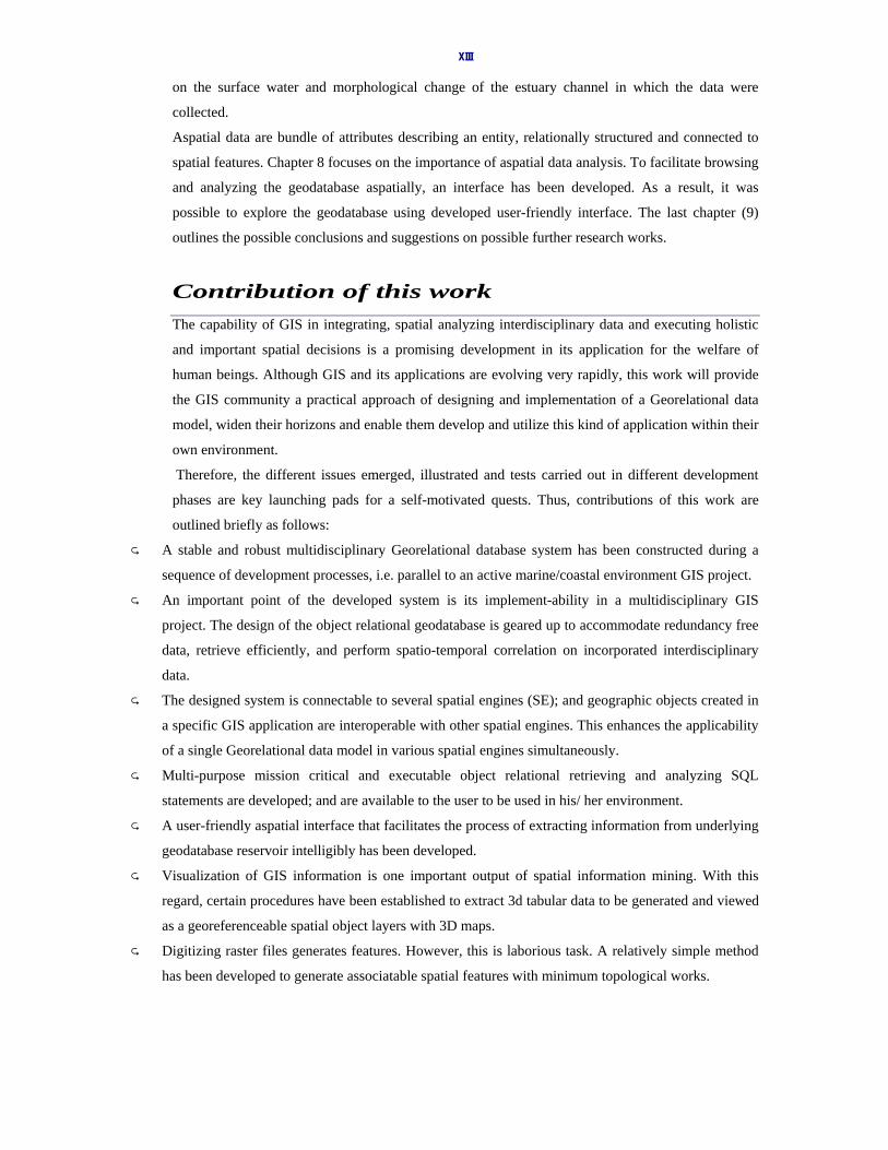
Aspatial data are bundle of attributes describing an entity, relationally structured and connected to

spatial features. Chapter 8 focuses on the importance of aspatial data analysis. To facilitate browsing

and analyzing the geodatabase aspatially, an interface has been developed. As a result, it was

possible to explore the geodatabase using developed user-friendly interface. The last chapter (9)

outlines the possible conclusions and suggestions on possible further research works.

Contribution of this work The capability of GIS in integrating, spatial analyzing interdisciplinary data and executing holistic

and important spatial decisions is a promising development in its application for the welfare of

human beings. Although GIS and its applications are evolving very rapidly, this work will provide

the GIS community a practical approach of designing and implementation of a Georelational data

model, widen their horizons and enable them develop and utilize this kind of application within their

own environment.

Therefore, the different issues emerged, illustrated and tests carried out in different development

phases are key launching pads for a self-motivated quests. Thus, contributions of this work are

outlined briefly as follows:

A stable and robust multidisciplinary Georelational database system has been constructed during a

sequence of development processes, i.e. parallel to an active marine/coastal environment GIS project.

An important point of the developed system is its implement-ability in a multidisciplinary GIS

project. The design of the object relational geodatabase is geared up to accommodate redundancy free

data, retrieve efficiently, and perform spatio-temporal correlation on incorporated interdisciplinary

data.

The designed system is connectable to several spatial engines (SE); and geographic objects created in

a specific GIS application are interoperable with other spatial engines. This enhances the applicability

of a single Georelational data model in various spatial engines simultaneously.

Multi-purpose mission critical and executable object relational retrieving and analyzing SQL

statements are developed; and are available to the user to be used in his/ her environment.

A user-friendly aspatial interface that facilitates the process of extracting information from underlying

geodatabase reservoir intelligibly has been developed.

Visualization of GIS information is one important output of spatial information mining. With this

regard, certain procedures have been established to extract 3d tabular data to be generated and viewed

as a georeferenceable spatial object layers with 3D maps.

Digitizing raster files generates features. However, this is laborious task. A relatively simple method

has been developed to generate associatable spatial features with minimum topological works.

XIV

G: Universal gravitational constant

Fg : Gravitational force

M1, M2 : Masses of two objects

s

to d2

R: separation between two object

d1, d2: distances changes from d1

ly: light year (astronomical unit)

XV

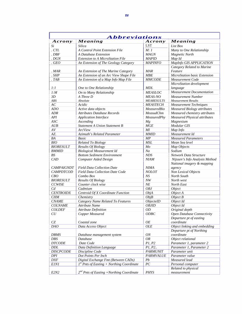
AbbreviationsAcrony Meaning Acrony Meaning

Si Silica LST List Box . CTL A Control Point Extension File M: 1 Many to One Relationship . DBF A Database Extension MAGN Magnetic North . DGN Extension to A MicroStation File MAPID Map Id . GEO An Extension of The Geology Category MAPINFO MapInfo GIS APPLICATION

. MAR An Extension of The Marine Category MAR Category Related to Marine Feature

. SHP An Extension of an Arc View Shape File MBE MicroStation basic Extension

. TAB An Extension of a Map Info Map File MMCODE Measurement Code

1:1 One to One Relationship MDL MicroStation development language

1:M On to Many Relationship MEASLOC Measurement Documentation 3D A Three D MEAS-NO Measurement Number ABS Absolute MEARESULTS Measurement Results AC Acidic MEASTECH Measurement Techniques ADO Active data objects MeasuredBio Measured Biology attributes ADR Attributes Database Records MeasudChm Measured chemistry attributes API Application Interface MeasuredPhy Measured Physical attributes ASC Ascending Mg Magnesium AUB Statement A Union Statement B MGE Modular GIS AV ArcView MI Map Info AZ. Azimuth’s Related Parameter MMID Measurement Id BA Basic MP Measured Parameters BIO Related To Biology MSL Mean Sea level BIORESULT Results Of Biology Mo Map Objects BMMID Biological Measurement Id Na Sodium BS Bottom Sediment Environment NDS Network Data Structure CAD Computer Aided Design NIAM Nijssen’s Info Analysis Method

CAMPAIGNDT Field Data Collection Date NIMA National imagery & mapping agency

CAMPDTCOD Field Data Collection Date Code NOLOT Non Lexical Objects CBO Combo Box NS North South BIORESULT Results Of Biology NW North west CCWISE Counter clock wise NE North East Cd Cadmium OBJ Object CENTROIDX Centroid Of X Coordinate Function ObjA Object A CHM Chemistry ObjB Object B CNAME Category Name Related To Features ObjecteID Object Id COLNAME Attribute Name OBJID Object Id COLDEF Attribute Definition OD Original depth CU Copper Measured ODBC Open Database Connectivity

CZ Coastal zone OE Departure pt of easting coordinate

DAO Data Access Object OLE Object linking and embedding

DBMS Database management system ON Departure pt of Northing coordinate

DBS Database OR Object relational DTCODE Date Code P1, P2 Parameter 1, parameter 2 DDL Data Definition Language P1, P2.. Parameter 1, Parameter 2 DISCPCODE Discipline Code PARMUNIT Parameter unit DPI Dot Points Per Inch PARMVALUE Parameter value DXF Digital Exchange Fmt (Between CADs) Pb Measured lead E1N1 1st Pnts of Easting + Northing Coordinate PC Personal computer

E2N2 2nd Pnts of Easting +Northing Coordinate PHYS Related to physical measurement

XVI

EBB.PARAM Ebb Related Parameter PMMID Physical measurement id

ECHODEPM Echo Sounding Measured Depth in Meters PSAD56 Provisional S_American Datum 1956

ECODE Estuary Data Code PT. Point ENTNM Entity Number PHS Primary hazard site ER1 Entity Relationship Rule R.S Results.Station EstChannels Estuary channels RCV Representative Class value E-W East to West RDBMS RD management system EXP.FILE Exportable File RDS Relational data structure φ Latitude REC-NO Record number (rec_no) F (T) Function Of Time REL Relation F (t) A Function of Time RESULTID Result Identifier F.F Field.Fieldcode RDS Relational data structure F-CODE Field Code of an Entity RSE Relationally structured entities FEATUREID A Feature Identifier S1, R1 Site1, Record 1 FIELDDATA Field Data S1, S2 Site2 Site 2 FK Foreign Key S1R1 Station 1 record 1 FDCODE Field Data Identifiers SA Spatial Analysis FMT Format SAMPDEPM Sample depth in meters FTDESC Fault description SAMPTIME-E End Of Sampling Time GCOORD Geocoordinator SE South East GeoLithology Lithology SED Sedimentology GEOREFNO Georeferenced Number SEDRESULT Results Of Sediments GeoTectonics Tectonics SGE System generated entities GIS Geographic Information System SILTPERC Silt Percent gm/l Micron Grams Per Liter SL Similar line works GPS Global position system SMMID Sedimentology id GVAL Gap Value SO Spatial objects HDS Hierarchical Data Structure SQR Square root Hevymet Heavy meta object SQRT Square root Hg Mercury Measured STC Space Time Composite I.O.C.A Oceana graphic de la Armada SW South West I: 1 or M: 1 One to One or Many to One SYStab System tables IGIS Integrated Geographic Information System T1 (L1) Layer 1 At Time 1 IMS Information management structure TAB Extension of MapInfo map INDVALUES Individual values TALIAS Table Alias ISD Information structure diagrams TbA Table A In Information at point TbB Table B JDBC Java database connectivity TCODE Tectonic structure code K Potassium TMS Temporal Map Sets λ Longitude TOLVAL Tolerance Value L1, L2 Layer 1, Layer 2 TSQL Transform SQL LAT Latitude UDE User Defined Entities LATDEGDEC Latitude Degree Decimal UDF User defined function LATTXT Latitude In Textual Form UDT User defined type

LBL Label UG-TAE-CAT System table compatible to MGE GIS

LCODE Lithology Code UMF Ultramafic composition LF Line Fragments URL Uniform Resource Identifier LITHID Lithology identifier UTM Universal Transverse Mercator LLE Longitude, latitude elevation VB Visual basic LOCATIONIDX Location Index WC Water Column LocID Location identifier WGS84 World geodetic system of 1984 LOCID Location Id WSI Eater Sediment Interface LON Longitude Z1, Z2 Zone 1 and zone2 LONDEC Longitude Decimal ZCODE Zone Code LONDEG Longitude Degree ZN Zinc LONTXT Longitude Text LST List Box LONTXT Longitude Text M: 1 Many to One Relationship LOT Lexical Objects MAGN Magnetic North

XVII

LS Line Segmentation MAPID Map Id Si Silica MAPINFO MapInfo GIS application

SOF Spatial Query Formulation MAR Category Related to Marine Feature

. CTL A Control Point Extension File MBE MicroStation basic Extension

. DBF A Database Extension MDL MicroStation development language

. DGN Extension to A MicroStation File MEASLOC Measurement Documentation

. GEO An Extension of The Geology Category MEAS-NO Measurement Number

. MAR An Extension of The Marine Category MEASRESUL Measurement Results

. SHP An Extension of an Arc View Shape File LST List Box

. TAB An Extension of a Map Info Map File MDL MicroStation development language

SYZYGY Alignment of the sun, moon and earth during spring tides QUADRATURE

In astronomy, arrangement of two celestial bodies at right angles to each other as viewed from a reference point. If the reference point is the earth and the sun is one of the bodies, a planet is in quadrature when its elongation is 90°.

http://www.infoplease.com/ce6/sci/A0817189.html

Chapter 1 1

Chapter 1: General Introduction

1.1. Introduction The coastal zone is an area at the edge of the oceans, which extends from the continental shelf to the

coastal plain [1]. Environmentally, it constitutes diverse habitats, major settlements, and significant

resources and socio-economically; it is the center of vibrant activities. It is marked by great

environmental instability effects such as sea level rise, geologic, geomorphologic and Sedimentological

changes. Moreover, it is a geographic center where a coastal zone shoreline is marked by prolonged

fluctuations of high/low tides. Understanding the magnitude and geographic scope of the changes and

effects might be difficult due to the cumulative processes of: - (i) Socio-economic activities impacts (ii)

Periodic environmental fluctuation and (iii) Intensive interaction among marine forces such as tides,

waves, winds, currents, etc.

i) Socio-Economic Activities Impacts: At the present time, the coastal ecosystem is being stressed

mainly due to higher population pressure compared to inland areas of the world. The related effects are

diverse and include polluted runoff (hazardous chemicals) into an estuarine environment ecosystem and

indiscriminate fishing (depletion and extinction of species)…etc.

ii) Periodic environmental Fluctuation: Although natural hazards have occurred throughout history,

their recent impact is becoming increasingly devastative along low lands of coastal zones.

iii) Interaction of Marine-Coastal Forces: The back and forth migration of shorelines results in

reshaping coastal geomorphology. These changes can pose a threat to the coastal community; and efforts

to manage problems associated with coastal resources, environment, population, uncontrolled

degradation pertaining to urbanization and their current potential relationship to sustainable

development of coastal resources has become wakeful issue [2]. Such changes related to the process can

be detected in images acquired through environmental satellites, for instance the Massive Iceberg Peels

off from Antarctic Ice Shelf [4].

One way of challenging the problem is establishing well Designed GeoRelational GIS Database

pertaining to a multidiscipline marine or coastal environment for an effective and efficient access and

managing the data spatially using Geographic Information System (GIS).

GIS is realized as an integrating, analyzing and visualizing tool for heterogeneous multidisciplinary

data within a system. This is due to the fact that, multiple information layers can be filtered and

analyzed to retrieve geo-referenced information, which are critical for decision-making. Thus, GIS is

becoming a vital tool for challenging issues that require spatial identification, interpretation and

assessing certain impacts [3] and vulnerability in the coastal zone. The application of GIS is increasing

across different disciplines. For instance, satellite images are available at a reasonable price and can be


Chapter 1 2

processed adequately to identify the evolution of deforestations or desertification. Further, GIS

associated with remote sensing can be exploited in mitigating and minimizing environmental

catastrophes (such as natural hazards-cyclones, floods etc) perform integrated coastal zones spatial

analysis and visualization of variety problems connected to the above stated issues (i-iii).

Motive: GeoRelational GIS DatabaseConstruction and Implementation

Process

MultidisciplinaryData

Aspatial DataStructuring

Entities andAttributes

Spatial DataStructuring

GeoreferencingTopology, Object

CreationDatabase Creation

Constraints

Spatial AnalysisOverlay AnalysisTrend AnalysisVisualization(2D And 3D)

InterpretationResults

Yes Yes

RECOMMENDATIONSDECISIONS

Yes

AssociationProcess

Point, Line,Polygon, Image

Anomaly DetectionZone Delineation

GeoRelational GIS

Interoperability

1.1.1 Motivation

An important derive behind this quest is founding of a functional GIS data model. The know-how on

how it is methodologically organized in space and time is fundamental to the development and

implementation of a Geodatabase. Without including multidisciplinary raw input data in a model, it

becomes rather difficult to reason about the dynamics of the real world spatial objects (SO).

Appropriate management and utilization of the miscellaneous data necessitates constructing a data

model that enables retrieving relevant information and performing a spatial analysis on

multidisciplinary data. Encrusting this notion in mind, the designed model is to be tested and

implemented across different GIS applications to assert its flexibility. Furthermore, the goal would

encompass performing spatial information

analysis on associated GIS building block

objects. This would include, discovering the

distribution rate of sediments and related

anomalous concentration (PCBs and heavy

metals), delimitation of abnormal

environmental spatial symptoms and

impacts discerned on biodiversity

distribution across the coastal environment

and understanding the process of tide

generation and effects on the current’s

velocity and direction.

Figure: 1-1 Motive : Georelational GIS

Construction

A graphical display of the intended motive

of this PhD research work is portrayed,

(see figure 1-1).

Moreover, decipher the hydro dynamics,

related to ebb and flows (current speed and direction) along estuary channels, perform spatial

correlation on the coastal geotectonic and GeoLithology on preexisting data, and thereby understand the

origin and relationship of the estuary channels (using a case study) to the coastal geology. Furthermore,


Chapter 1 3

perform Spatio-structural analysis on the tectonic trends to deduce tectonic alignment to the regional

structures, which is an essential step in assessing seismicity in the coastal zone of Guayaquil.

1.1.2 Problem Statement

Problem statement: The coastal zone is a dynamic environment and is essentially known as a source of

interdependent data. Data is powerful asset if managed appropriately by well established geodatabase.

Building a robust and implemental GeoRelational GIS data model is rather an overlooked challenged.

Connecting with this, implementing one and the same geodata model across different GIS applications

is very important, although, that but it requires a persistent efforts and resources to achieve it.

Conceptual Solution: Environmentally the coastal zone (CZ) can be subdivided into, (A) coastal

geology comprised of Lithology and Tectonic Structures (B) Main estuary, mainly of surface water, and

deep water which are associated different sediment particles. Based on these and other data categories, a

vector GeoRelational GIS Data model applicable in coastal zone/marine environment can be devised

and implemented. Spatial analysis can be performed to correlate events associated to the main estuary

and coastal zone through thematic and spatial coincidence of multidisciplinary geographic objects. This

would enhance understanding the relationship of estuary and Coastal GeoTectonics structures play vital

role in producing a priority search maps, locating (delimiting) environmental anomalies and assess

relevant potential resources.

1.1.3 Research Objectives

Model, Design and Implement a Geo-Relational Multidisciplinary GIS Database for the Application of

a Marine / Coastal environment across different GIS applications

Devise a plausible definition and populating methodology for conceptually and realistically structured

Multidisciplinary objects.

Integrate and link spatially diverse measurements data (biology, Sedimentology, physic-chemical

…etc.) and build up geo-reference-able and topologically cleaned coastal GIS maps which are

applicable across different GIS engines.

Validate and evaluate the reliability of graphic and tabular outputs utilizing Object Relational Spatial

Operators. Develop an aspatial interface that enable process and manipulate the data.

Harness complex sub-queries, spatial analysis akin to buffering, overlay and statistical delimited spatial

anomalous zones on the Geo-Relationally interconnected coastal objects.

Visualize the coastal zone via constructed 3d maps and associated Meta data.

1.1.4 Research Questions

Major questions addressed in this thesis work include: -


Chapter 1 4

How to organize, design and implement multidisciplinary data for the development of coastal/ marine

Georelational GIS

How to structure /define interdisciplinary entities that converge and share identical dereferencing

position

How to assimilate user defined objects, special system generated object; establish cardinality that

functions in object relational GIS data models.

How to construct interoperable Geographic objects with or without preserving its object properties

How to synchronize objects with a 1: M relationship in order to achieve thematic analysis results.

How to develop object Relational spatial queries and perform spatial analysis aimed on detecting

coastal environment impacts and trends

How to construct a 3D map and integrate with geo-referenced geographic objects

How to create and integrate Meta data (video, images and documents) with spatial objects and employ

them during the phase of data mining and thematical visualization

1.1.5 Scope of the Research

Modeling, Design and Implementation of a coastal/marine GeoRelational GIS database

Design Method of Generating and Integrating of multidisciplinary geographic objects

Technical tools development of topological clean up tools

Design of spatial query and analysis for employment among different geographic object types

Practical Interoperability operations and Communication of the model among GIS engines

Object Relational data mining methodology on Objects applying object operators and object Identifiers.

Development of spatial and aspatial interfaces

1.1.6 Methodology

Conceptual Geodatabase design: Conceptual entities design was carried out by establishing rules

(proposition) of communications based Nyssen Information Analysis Method [33]. Abstractly, the rules

link the entities and the information structure diagram conforms to the communication rules.

Physical implementation: Entities and attributes were physically created applying a Data Definition

Language (DDL) and the DAO (data access object). Data types and constraints among the conceptual

building block entities established. Graphic representation and cardinality of the structured geodatabase

was generated using a case tool (Visio Professional). Data types applicable at this phase were

alphanumeric and date and the possible entity pointers were determined.

Objects Definition and Topology: The geometric objects (Points, lines and shapes) executed using

MicroStation basic extension (MBE), [12] and Mapbasic, [36] programs. Furthermore, Digitizing

process was applied to create geometric features within a geo-reference-able map. Also, spatial update

operations on a generated object were applied to create new objects. E.g., a series of x, y coordinate

based object points were converted into a Polyline type by updating the point object. Topological


Chapter 1 5

operations were performed to clear undesired line works and create shapes required for thematic

resymbolisation.

Interoperability: The constructed GIS geodatabase has been set to communicate with different spatial

engines. (Geographics [11], ArcView [21], MapInfo, [30] and ArcGIS [89]), Connected via compatible

DLLs and ODBC version.

Also, experiment on interoperability among the spatial engines executed based on transforming and

employing a specific GIS application feature into another GIS application. (For instance MicroStation

Geographic DGN files into ArcView GIS shape file, or MapInfo tab file into ArcGIS shape etc.

The process necessitates an appropriate definition of the original feature and feature translation. The

interoperability experiment shows loss and preservation of feature property during the spatial

information exchanging process. E.g., object identifier of MicroStation Geographic changed into

MapInfo object identifier with certain object id prefix.

Geo-reference: Requires availability of a known ellipsoid, datum and a target map. A grid map that

conforms to a target map was generated applying projection application Geocoordinator. It was

implemented using a projection system of universal transverse Mercator (UTM) and a datum known as

PSAD56.

A satellite image related to the same target area and same datum has also been available. Reregistering

it using control points, applying the same datum, and corresponding to known points of reference has

proved a successful geo-referencing and superimposition of both types of GIS maps.

Spatial interface and spatial interpretations: Every GIS application presents its own interface to the

user. Some are very user friendly and others are relatively not. A customized interface for incorporating

spatial layers and connecting to the geodatabase has been developed. This has been done applying

ArcGIS and Visual basic (VB6) and Map objects (MO), [70]. Its functionality facilitates adding maps

and connecting to the Geodatabase. Since its interface functionality is already in the GIS application, it

is skipped.

Spatial interpretation process has been executed by designing object relational spatial queries. This

process includes (a) on the objects themselves (b) object identifiers and (c) type of the objects (d)

sharing of the same geo-referencing properties. The later has been vital for extraction of the spatial

information on the coincidence of the geographic objects boundary and centroids. A hybrid of spatial

and SQL operators (contain, intersect, within, overlays…etc.) were incorporated with a SELECT query

structure.

Aspatial interface: An object oriented programming environment Visual basic [74] has been applied

to develop an aspatial interface using procedures and program codes. The Aspatial interface-building

components include - VB forms, controls connected to the underlying procedure program codes and

embedded queries. The interface facilitates the performance of visual analysis of the underlying

Geodatabase data without writing SQL codes and connecting to different GIS applications.


Chapter 1 6

1.2. Background

1.2.1 Conceptual Definition of (GIS)

In most cases Geographic Information System (GIS) is a computer based information system used to

digitally represent and analyze the geographic features present on the Earth' surface and the events

(non-spatial attributes linked to geography elements). Every object present on the Earth can be geo-

referenced, is the fundamental key of associating any database to GIS. GIS stands for Geographic

Information System. Its perception can be paraphrased as follows: -

Geographic: Signify spatial features. Real world objects (features) referenced to a particular location in

space [6]. For instance, the different features (lines, points, polygons …etc.) on a map depict graphic

representation of real world objects. The spatial objects are represented by different symbology (color,

line weight and styles).

Information: It is a processed data converted to meaningful form through analysis [12].

Systems: A term utilized to indicate the systems approach taken by the GIS, where complex systems

are decomposed into their component parts for ease of understanding and managing. GIS encompass the

storage systems, processing and manipulation of tools, projection systems. In other words, a GIS is both

a database system with specific capabilities for spatially referenced data [7]. It is defined as a powerful

set of tools for collecting, retrieving, at will, transforming and displaying spatial data from the real

world [54].According to [21], a Geographic Information Sys tem is a computer-based tool for mapping

and analyzing things that exist and events that happen on earth. GIS Technology integrates common

database operations such as query and statistical analysis with unique visualization and geographic

analysis benefits offered by maps. These abilities distinguish GIS from other information systems and

make it valuable to a wide range of public and private enterprise for explaining events, predicting

outcomes, and planning strategy.

1.2.2 Evolution of GIS

The evolution of manual GIS system was derived from the discipline of cartography [7], as site

designers and architects required visual comparison and contrast the building plan with the site surveys.

These were translucent papers and later plastic sheets upon which maps were drawn or printed. For

instance, a map of a drainage site can be overlaid on a topographic map or a street plan. These layers of

information could help a site or urban planner to determine whether or not to locate houses or other

buildings at a given place. An information layer is mostly like a conventional map, flat drawing

indicating the nature, form, relative position and the size of the selected geographic area. A typical

overlay map includes several layers. Likewise, overlay layers (see figure 1-4) can be used to interpret


Chapter 1 7

different information layers; example, geo-chemical data over mineralized rock super imposed on a

satellite images.

1.2.3 GIS System Ingredients

A) Engines: Two main systems are involved in a dual architect GIS database; these are DBMS

(database management system) and graphics systems. The database is separated from the spatial engine

because the relational database stores the textual information format and the graphic with different

format. Textual data are stored and retrieved more efficiently the RDBMS. Further, the data in the

database becomes easily available for sharing with other software applications. An API is applied to

create the connection, transfer and process of data. However, the retrieving process subsumes migrating

spatial pointer to extract spatial information. Typical types of GIS with such architecture are, Modular

Geographic Information System (MGE), [20], MicroStation geographic [11], and MapInfo professional

Version [30]…etc.

Other GIS alternatives that encompass both engines in a single system are known as integrated GIS

(IGIS) system. For instance, some of the currently active integrated GIS management engine types

(IGIS) include Oracle spatial cartridge [90], Informix spatial [91], DB2 spatial extender [92].

B) Interfaces: Windows is fundamental for the display of the processed information within the

computer.

C) Hardware: machinery on which a GIS operates such as a computer, printer, plotter, scanners and

digitizers. Includes workstations and networks for communication with other systems, disks, and tape

for storage and digitizers for creating vector objects, see Figure 1-2.

D) People: - The most important of GIS; without people GIS will not work. To be useful and successful

it should have people dedicated to it. System user: is responsible for the day-to-day operation of the

system, engages with trouble shootings and system hang-ups, train and configure systems, act as system

as well as database

administrator whereas

GIS suppliers: are

responsible for the GIS

software provision.

Figure: 1-2 GIS Physical

Component

GIS system analysts: are group of people specialized in the study of systems design, professional

responsible for determine the goals and objectives of the GIS system within the organization.


Chapter 1 8

E) Data: GIS can use data from a wide variety of proprietary and standard maps and graphic formats,

cad files, spread sheets relational database sources.

Figure: 1-3 GIS Ingredients

1.2.3.1 Spatial Engine Functions

A GIS engine has the capabilities of data capturing, storage, data editing, management, retrieval,

analyses and display. GIS can detect and eliminate (capturing and editing) digitized errors, which are

one of the essential functions in editing of maps, for example in [19] and [20], a GIS function can snap

nodes so that points that are close to each other are automatically placed with identical co-ordinates

Shape Creation: Topological based GIS applications can check for gapped nodes, dangles, and

duplicate lines and eliminate unnecessary map elements (see chapter 4). Automated cleaning should be

carried out cautiously because the assigned tolerance may eliminate important topological elements.

Choroplethic Mapping: -Choroplethic Mapping is the display of mapped area based on classes of

attribute values. A legend acts as a lookup table with each range of attribute values being associated

with particular color of the distribution of attribute values, E.g. dispersion rate of Hg (mercury in

different areas) in a specified location and depth (see chapter 6). Spatial Analysis requires linkage

(assimilation) between the spatial features and the attribute data bounded to the same coordinate

performed by a process of projection (see chapter 5). Queries on a GIS can thus be Graphic driven or

Data Driven. Graphic driven queries involve spatial features based on searches for objects and retrieval

of the associated attribute data, and query functions to select features and retrieve the associated

information (see chapter 6).

Buffering: GIS performs analysis based on zonal boundary generation with reference to a spatially

associated feature (s) (lines, points or areas) at a specified distance. The distance is set from the

original object during a spatial analysis e.g. creation of buffer zone around measurement location to


Chapter 1 9

display the concentration of pollutants dissemination intensity 50 meters away from the foci of the geo-

referenced point.

Overlay Analysis: Shape features of specific data layer are overlaid onto those of other data layers in

order to calculate the areas, which have a certain combination of attribute values or lack of common

values.

E.g., overlay of geo-chemical distribution of the heavy metal lead concentration feature display over

the underlying geological rocks.

Depending on the provenance of base metals then relationship of the dispersion of the geo-chemical

elements can be related and interpolated directly to its main underlying source.

1.2.3.2 Database Engine Functions

Data Definitions, Manipulations and Integrity Checkups: In order to make a GIS useful, the database

manager checks the attributes integrity, enforce restrictions on the GIS that specified during the data

definition phase of the database construction, (see chapter 2).

The Database management system (DBMS) allows the manipulation and retrieving of information and

supports tabular or other list types of output. Much of the power of the GIS software is generated from

the ability to manage not just map data but also associated attribute data, stored in the DBMS.

1.3. Measures and Solutions Many spatial and aspatial problems can be handled if the development applications are known to some

extent to the user. The measures should include measurements related to spatial technology for

establishing spatial database that lead to appropriate assessment and monitor the environment.

The data (spatial and aspatial must be modeled by incorporating with appropriate geographical

coordinates [5] and temporal time-stamp.

Thus, integrated multidisciplinary data modeling is key approach to the possibility of appropriate and

holistic geographic analysis to obtain predictable results in order to understand the genesis of natural

phenomenon and protection of vital coastal eco-system.

1.3.1 Data Acquisition


Chapter 1 10

Integrated Monitoring: Regular assessments of environmental issues in coastal zones using integrated

environmental GIS database management analysis and visualization of the multidisciplinary data sets

enhance monitoring effects and response on coastal environment.

GIS related researches aimed on collecting integrated multidisciplinary data set (geological, biological,

physical, geo-chemical and digital spatial data) and integrating with pre-existing data using Geographic

Information System facilitate the holistic spatial analysis, decision making on monitoring performance

of the coastal zone environment.

Analysis and Display: GIS has the power and capability of being queried and display geo-referenced

information. Furthermore, it can integrate multidisciplinary data layers and view the extracted

information in a holistic perspective, (see figure 1-4). Geolithology (rocks) affected by different

magnitude of geotectonic structures, bathymetric contour and measurement stations layers are depicting

the processed data layers and all are bound to the same geo-referencing grid. GIS enables not only

process the tabular data but also monitor and analyze socio-economic and environments repercussions

by means of Choroplethic maps, 3D visualization and integrated statistical trend graphic displays.

Figure: 1-4 GIS Information Layers

1.3.2 GIS Objects Models

The principle of data modeling is based on the concept that all objects should be clearly defined. The

first point is how to define an object in a dual GIS database. Two diametrically opposed geographic

data models (vector and raster) are available nowadays for encapsulating the aspects of interest of

spatial phenomenon. In the vector model, lines link a series of exactly known points and exactly defined


Chapter 1 11

lines bound polygons. The raster object based model regards spatial data as a cell grid at a given level

of resolution. Figure 1-5 shows a common raster and vector data models where the grid is represented

by fixed sized pixels. These two models are abstraction of reality that appeals for their logical

consistency and their ease of handling using conventional reasoning [69].

Figure: 1-5 GIS Models ( vector and raster)

The advantage of vector (feature) object models is that the topological relationship can be expressed

explicitly; however, it lacks the handling of continuous objects. The advantage of a raster lies on its

capability to handle the continuity of spatial objects; however, it lacks a definite form of boundary.

Point – (Location site): composed of x and y coordinates, is the simplest graphical representation of an

object. Its visibility depends on the viewing scale. A point feature class has been used to represent a

measurement site during the construction of the Geodatabase in this research work.

Lines- (Area boundary): - composed of x1, y1 and x2, y2 coordinates, represents one-dimension

objects. Lines connect at least two points and are used to represent objects. For the coastal environment,

GIS (Guayaquil estuary) line features were applied as bounding geographic features.

Polygon – (An area of interest): composed of a series of x1, y1, x2, y2, x3, y3 and x1y1 coordinates.

Polygons represent geographic objects defined in two dimensions. It is represented by at least three

connecting lines, each of which comprises of points. In this work, polygons represent the delineated

zone of a coastal zone environment and Lithology covered by specific composition. Adding the

elevation (z) to an area feature allows us to observe and record information in 3D (see figure 1-6).


Chapter 1 12

Figure: 1-6 Geometric elements

These (points, line, polygon) are major building blocks of spatial elements of a vector based GIS where

their generation depends mainly within the spatial engine and the type of a seed file [7].

Figure: 1-7 Type of Data Incorporated

Besides the spatial objects, data available for the case study and research work encompasses data

collected insitu during a measurement field works from disparate locations and pre-existing documents.

They are classified as primary and secondary type to indicate originates of data acquired as indicated in

figure 1-7.

1.3.3 Approaches in the Application of GIS

1.3.3.1 Environmental Approach

The strength of GIS is based on its capability of integrating multiple disciplines and permitting the user

to inter-relate and correlate the processed data with respect to a geo-referencing point. However, the

complex nature of multidisciplinary data in general and the coastal environment data in particular

requires rigors analysis before incorporated into a structured GIS database [7].


Chapter 1 13

Figure: 1-8 Environmental

Assesment

Purpose: - Clearly

defined purpose is

required to harness

GIS as a supportive

tool for targeting

vulnerable locations

and applying for hazard mitigation. Figure 1-8 shows the required general environment assessment.

Detection of Sources data: - Identify areas susceptible to primary hazards sites (PHS) in relation to

most possible natural hazardous regions and design hypothetical inquire.

Identify key environmental resource: - locations and their proximity to secondary risk sites

(prioritize secondary risk sites). Examples: a) after flooding, dams may burst and inflict an adverse

environment on areas rich in vulnerable community. In this case, census on a bio-diversity is important

in identifying endangered species per area.

Suggested GIS Solution: - Overlay species maps per area may show either flourishing or extinction

trend of the flora and fauna.

1.3.3.2 Economic Approach

Identifying economic zones, which are categorized to be potentially vulnerable to hazard impacts?

Mapping primary centers of activity and assess major possible impacts on local economy and public

properties. For instance, floods cause disasters [42], whenever a river overflows its banks; it dumps

sediments and debris on to the surrounding land (see figure 1-9b).


Chapter 1 14

Figure: 1-9 Economic Assessment (a) Flood disaster in Europe (b)

Required considerations include (see figure 1-9a), identify and locate primary economic sectors, which

are vulnerable to hazard impacts, mapping primary centers of activities and assessing major possible

impacts on public properties and Identify linkages of economic core and high-risk areas.

1.3.3.3 Societal Approach

Identifying inter-relations of special consideration areas with high-risk, such as locations where

individual’s personal resources for dealing with hazards can be extremely limited.

Figure: 1-10 Societal assessment

Figure 1-10 illustrates the

processes of gathering

data and possible

outcomes of the process

during the application of

GIS in finding solutions

to social problems.

Suggested GIS

application Solution: =

Spatial Maps supported by ranked values will indicate areas that require prime priority. Use Overlay

and spatial analysis methods by taking into account special areas of special considerations

1.3.3.4 Hazard Approach

Extract all possible and best available information to identify higher potential impact areas as a

repercussion of each hazard. For instance, locating target areas liable to flooding or storms, burst of

polluted fluids; earthquakes on slop stability …etc. and categorize them in degree of different level of

risk intensity.


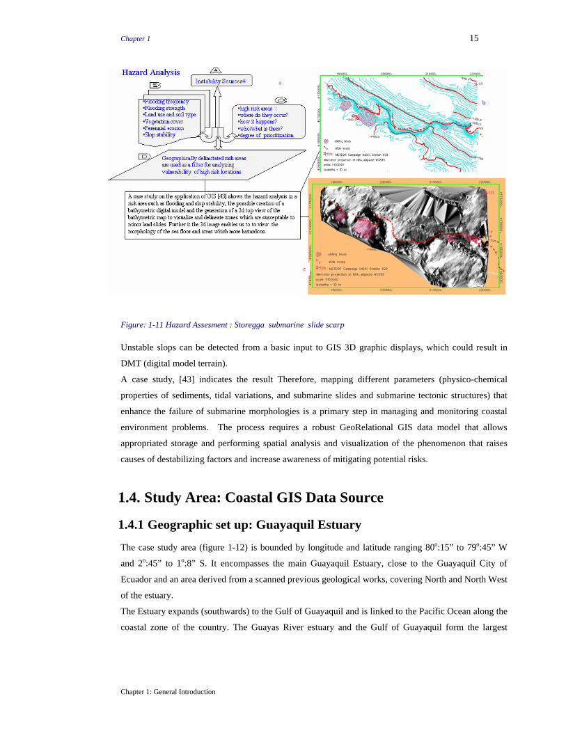
Chapter 1 15

Figure: 1-11 Hazard Assesment : Storegga submarine slide scarp

Unstable slops can be detected from a basic input to GIS 3D graphic displays, which could result in

DMT (digital model terrain).

A case study, [43] indicates the result Therefore, mapping different parameters (physico-chemical

properties of sediments, tidal variations, and submarine slides and submarine tectonic structures) that

enhance the failure of submarine morphologies is a primary step in managing and monitoring coastal

environment problems. The process requires a robust GeoRelational GIS data model that allows

appropriated storage and performing spatial analysis and visualization of the phenomenon that raises

causes of destabilizing factors and increase awareness of mitigating potential risks.

1.4. Study Area: Coastal GIS Data Source

1.4.1 Geographic set up: Guayaquil Estuary

The case study area (figure 1-12) is bounded by longitude and latitude ranging 80o:15” to 79o:45” W

and 2o:45” to 1o:8” S. It encompasses the main Guayaquil Estuary, close to the Guayaquil City of

Ecuador and an area derived from a scanned previous geological works, covering North and North West

of the estuary.

The Estuary expands (southwards) to the Gulf of Guayaquil and is linked to the Pacific Ocean along the

coastal zone of the country. The Guayas River estuary and the Gulf of Guayaquil form the largest


Chapter 1 16

estuarine ecosystem on the Pacific coast of South America [95], and it is an important sanctuary for

habitat and economically important marine invertebrates.

According to [96], the river-dominated estuary of Guayas has a tidal range of 3-5 meters compared to

the tidal range of 0.25 to 0.5 through out the Caribbean. This regional setting is classified as

allocthonous coasts with strong tidal currents.

Furthermore, the rainfall in the area is seasonal, with more than 95% of the precipitation occurring from

December to May causing seasonal river discharge ranging from 200 m3s-1 during an average dry

season to 1400 m3s-1 in the wet season during average year of precipitation [96]. The same literature

further indicates that the annual mean temperature varies from 24 to 27 (oC) along the coast resulting a

potential evapo-transpiration rate of about 1300 mmy-1.

The estuary acquires water from the perennial rivers that flow into and from the oceanographic

processes in the Gulf of Guayaquil, [14]. Two major channels of the Estuary are the Esterio Salado and

the Guayas River. The estuary occurs at the junction where the southerly tropical Current from the

Panama Bight and the northward flowing Humboldt Current from Peru. This current is what brought

Penguins and Fur Seals to the Galapagos [61].

This literature indicates that the dominance of the Panamanian current occurs during the summer

causing an increase in seawater temperature and initiates the onset of the rainy season. Years of

abnormally warm water temperature and associated rainfall attributed to the EL NINO climate pattern.

A research study reported in [15] depicts that warmer offshore waters resulted to the explosion of white

shrimp population off the coast from enhanced spawning and maturation. Geotectonically, a Regional,

a major fault system, known as the Delores-Guayaquil Mega shear, [97], on the gulf of Guayaquil

passes into the Interandean valley.

According to the literature the Delores-Guayaquil Mega shear is similar in scale and seismic activity to

the San Andreas Fault system in California. [97]. Such fault system has made the country exposed

continually to earthquakes and other geologic hazards, [98].

The north and northwestern part of the estuary is also characterized by multi-direction fault trends

indicating the geotectonic of the coastal region. The Progresso Basin in the Gulf of Guayaquil is

believed to have formed as pull-apart basins within the strike-slip regime of the Dolores–Guayaquil

Mega shear (DGM)


http://www.galapagosonline.com/Galapagos_Natural_History/Birds_and_Animals/Birds/Penguins.html

http://www.galapagosonline.com/Galapagos_Natural_History/Birds_and_Animals/Animals/Seals.html

Chapter 1 17

Figure: 1-12 Study area : The GeoData

1.4.2 Estuary

Description: The nature and organizations of facies within incised valley estuary is controlled by the

interplay between marine processes (waves and tides), which generally decreases in intensity up-

streaming, and fluvial process, which decreases in strength down estuary [101]. Further, the literature


Chapter 1 18

also illustrates that an ideal estuary posses a three-fold (tripartite) structures. These facial zones are: -

(a) an outer zone, which is a marine process dominated portion and the net bed-load is head-ward; (b)

central zone, relatively low energy, where there exist a net bed-load convergence and (c) inner zone: - a

marine dominated but river influenced where the net transport is seaward. However, all estuaries may

not show the same development mainly due to the availability of sediments, coastal gradients, and the

evolution of the estuary. Two distinct but intergradational types of estuaries (waves, and tides

dominate) are recognized based on the dominant marine process. The wave dominated estuaries

typically posses a well defined tripartite zonation: a marine sandy body barrier, wash-over, tidal inlet

and tidal delta deposit; a fine grained generally muddy (central basin); and a bay head delta that

experience tidal and saltwater influence. The marine tide dominated sand body consists elongated sand

bars and passes head into low-sinuosity or straight channel; equivalent to the central zone is described

by a tight meanders where bed-load transport by flood tidal and river currents is equal in the long term.

These ideal facies models and their conceptual basis provide means of highlighting the difference

between estuaries and the possibility of having a clear definition of an estuary.

Figure: 1-13 An Estuary’s dynamic view

Definition: Estuaries are dominant features along the modern coastlines, are results of Holocene

transgressions and some times are associated to tectonic structures filled by undifferentiated sediments.

They are strongly influenced by a seaward flow of terrestrial waters and by a landward surge of saline

ocean waters. These processes of mixing up of different water masses and different composition create

variation in the estuarine environment and Sedimentological depositions as indicated in the sketched

figure (see figure 1-13). The facies boundary marking the landward end of the estuary as defined always

lies landward of the 0.1%o salinity value but the facies boundary of the outer end may lie either

landward (as shown here) or seaward of the limit of normal marine salinities (32%0), (see figure 1-14).

The most widely used definition of an estuary is based on the salinity concentration, with specific

requirements and which states “a zone in the seaward river where the seawater is measurably diluted


Chapter 1 19

with water derived from land drainage” [102]. This definition implies that an estuary would occupy the

mouth of a river where the salinity ranges 0.1 to 30 ppt (see figure 1-14). This definition is useful when

dealing with chemical and biological process, in the fluvial–marine transgression. But it is of limited

use in the study of ancient deposits because the physical process rather than the salinity determines the

distribution of the lithofacises. On the other hand, defintions of an estuary include tides; for instance,

according to Fairbridge [104], an estuary is defined as “an outlet of the sea, reaching into a river valley

as far as the upper limit of tidal rise “ however this definition is argued, if strictly applied would

includes delta, barrier and lagoons as part of the estuary.

32%0 Salinity Facies Boundary Between EstuarineSand Body And Normal Marine Sediments

0.1%0 Salinity

Tidal Influence Limit

Fluvial Sediemnt

Facies boundary between Marine (tidally-)influencedand fluvial sediements

River ProcessesTidal Processes

Wave Processes

Marine Sediemnt

RiverEstuary(Pritchard,1967)Marine

Relat

ive en

ergy

(%)

50

0

100River CurrentsMarine Processes(Waves and Tides) Mixed Energy

Marine Dominated River DominatedRiverMarine

Central InnerOuter

Estuary (Dalrymple etal, 1992)River

I

II

Figure: 1-14 : I Estuary’s Definiton Schematic Representation ( Pritchard, 1967 )and Darymple et al., 1992).

Thus, the definition of estuary should include processes such as the river currents and marine process,

tides, waves as well salt-water intrusions. Based on these considerations - an estuary is the seaward

portion of a drowned valley which receives sediments from both fluvial and marine sources [101] and

which contains facies influenced by tides, waves and fluvial process, (see figure 1-14, II ).

In most cases, the fluvial energy, as given by energy influx per unit cross sectional area, typically

decrease downward of an estuary because the hydraulic gradient changes as the river approaches the

sea. Marine energy by contrast, generally decreases headword, either because the oceanic energy is

dissipated by wave built barriers or tidal speeds diminishes up estuary as a result of frictional damping.

Thus, Estuaries (marine influenced, seaward portion of a drowned valleys) are depostionally complex


Chapter 1 20

due to the interaction of river and marine (tidal or waves) processes. However, despite this, literature

study indicates certain organization of the estuaries environment due to the predictable nature of the

fluvial and marine intensities or the river and marine process. Coarse sediments supplied by marine,

river processes accumulates in the outer (marine dominated), and inner, (river dominated) portion of the

estuary respectively, while finer sediments occurs in the central zone. The nature of the sediments

depends on the nature of depositional environments (waves and tides), which are applied for the

purpose of classifying estuaries into wave and tide dominated. In an ideal wave dominated estuary, the

tripartite facies distribution is clearly expressed. An analogous tidal dominated estuary, clearly defined

zone is not possible because tides can penetrate the sediments more than the waves do. Most modern

estuarine differ from idealized models due factors such as the mixing influence of waves and tides,

variation in the coarse sediment supply by marine or river process and dimension of the valleys.

1.4.3 The GIS’s Raw Data Resources

Data employed during this research work have been obtained from a GIS project work conducted

during the 1996 and 1997, in the Guayaquil Estuary. The data constitutes a variety of measurement

data, temporal, images (scanned / satellite) and vector coastline maps.

Measurement data: multidisciplinary data pertaining to aquatic (extend from the estuary-water-

surface to estuary-bottom zone) environment (figure 1-15).

Figure: 1-15 Coastal Zone Environment Data Interaction (a) and GIS Data Input Scheme(b)


Chapter 1 21

The WC (water column) data is characterized by direct interaction with atmospheric and terrestrial data,

climatic change, coastal degradation and man made impacts respectively. This environment extends

vertically towards the (water sediment interface) WSI. The WSI is a benthic environment habituated by

benthos species and denser sediments particles. BS (bottom sediments) environment hosts muddy

sediments and organic material data, which can grade to undifferentiated bulk sediments, depending on

the state of the bottom estuary environment. The WC, WSI and BS are thought to have direct or indirect

interactive relationship with the coastal environment medium and coastal peripheral sediments can be

deposited within the WC-WSI-BS mediums (see figure 1-15).

The coastal data are complex. Figure 1-15(b) displays multidisciplinary measurement data incorporated

in the Geo-Relational GIS data Model of the Marine / Coastal GIS. This complexity necessitates the

Construction of Geo-relational data model for the appropriate storage, integration of spatial and aspatial

data and enhances analysis of various coastal phenomena.

It becomes evident if one takes into account factors such as the diversity of data resources related to

fishing, tourism, transportation, rhythmic motion of marine forces and heterogeneous constructions,

land use vs. misuse and consequences of industrial discharges into transitional water mediums

(estuaries). Implementing an integrated GIS database on data, acquired on regular span of time, better

image resolution and increased measurement density in a dynamic environment like an estuary

environment is indispensable to solve critical environmental problems.

Scanned Paper map data: They are maps derived from pre-existing geological reports [16] related to

the coastal peripheral geo-set-up (Lithology) and Tectonic structural. They have been registered and

vectorised before being incorporated to the geodatabase. The graphic data include bathymetric and

satellite images, as described in tables 1-1 and 1-2).

Table :1-1 Data source

The data has been obtained from the Instituto Oceanographico De La Armada (I.O.A.), 1976, Coastline

Ecuador: According to [95]. The Lithology of the coastal periphery is composed of typical coastal

deposition such as solidified carbonate rocks-limestone, argillite, greywacke, alluvial and colluvial

sediments [16]. The Peripheral Geology and Structural Data depicts that the area is composed of tertiary

sediments and the NW tectonic structures.


Chapter 1 22

Table:1-2

Measurement, Images

and Coastal Geologic

Document

1.4.4 Coastal GIS Data Composition

Various data were collected from the Guayaquil estuary, in different measurement stations with respect

to different depths during the 8th month of 1996 and 4th month of 1997 fieldwork by different scientists

for GIS related scientific research work. To facilitate the interpretation, the depths pertaining to the data

collected per station are categorized as surface water column (depth ranging 0.2 - 1.0 meter), middle

water column data (depth ranging 4.0-9.0 meters) and bottom water including the bottom sediments

(3.0-19.0 meters). Main components of the data include discipline specific entities such as Zoo and

phyto planktons, Bulk sediments, physico-chemical … etc., (see table 1-3)


Chapter 1 23

parameter unit parameter unit parameter unit parameter unit parameter unit parameteunit parameterunitAcartia spp. ind/m3 cadmium ug/l Abundance cel L1 clay % Nitrates μg/l ph ++ direction degMagAcrocalanus sp. ind/m3 chromium mg/kg Abundance ind.L-1 silt % Phosphates μg/l salinity ppt speed cm.s-1

Aegisthus ind/m3 chromium ug/l Abundance org/m3 sand % Silicates μg/l temp °CAppendicularia ind/m3 copper mg/kg Abundance net org/m3 gravel %Ascidian larvae ind/m3 copper ug/l Number of CountBivalvia ind/m3 mercury mg/kg Number of ind.L-1

Egg Pisces ind/m3 mercury ug/lForaminifera ind/m3 zinc mg/kgGastropoda ind/m3 zinc ug/lLarvae Pisces ind/m3Medusa ind/m3Mysids ind/m3Polychaeta ind/m3Rotifer ind/m3Tintinid ind/m3Tortanus sp. ind/m3total abundance ind/m3

Water CurrentBulk Sed

Physico chNutrients

Zoo planktonHeavy Metal

Phytoplankton

Table: 1-3 Coastal RawData Descriptive Parameters

Bottom Sediments: Data pertaining to the discipline Sedimentology, collected during the 1996 and

1997 GIS project field works were composed of bottom sediments, bottom water and surface water

environments. The bottom sediments data were approximately 21 samples and are of bulk sample type.

They are composed of unconsolidated sediments, organic materials and rock fragments.

The sampling technique applied includes Van Veen 5 kg, (A type of grab sampler for several sizes

sediments, especially applicable for collecting bottom sediments, (See figure 1-16 a).

The sampling depth environment of this data ranges between 3 and 19 meters. The analytic technique

has been carried out using R. Folk, Schla&Schm, 1969/pipette and R. Folk, Schla&Schm, 1969/sieve.

These bulk samples have been analyzed for the purpose of identifying Sedimentological processes,

compositions and perform spatial interpretation using GIS spatial applications.


Chapter 1 24

Table : 1-4 Bottom sediments

Heavy Metals: The data related to the discipline heavy metals, collected in the same duration of the

Sedimentological data belongs to the bottom water column environment. The data were of bottom

water sample type. The heavy metals analysis result is related to possible sources of a local galvanic

industry, natural set-up and gold mining environment. The sampling technique applied includes

Botella Van Dorn type, (Valve-closing bottle used to collect data), see figure 1-16) and Goulds NPE

pump, 2HP, 3450 rpm, 1 1/2 x 2” High Efficiency Impeller (turbine motion). The water samples

have been analyzed to gauge and identify the concentration (micro gram per liter) of the heavy metals

parameters of mercury, copper, zinc, chromium and lead, (see table 1-5).

Table: 1-5 Bottom Water Column Environment

Figure: 1-16 Van Veen Sampler

(a) and Bottela Van Dorn Veen

Sampler(b)


Chapter 1 25

Physico-Chemical: The physico-Chem. data collected during the same GIS project field works is of

water column environment type with a sampling depth environment ranging 0.2 to 15 meters. The

sampling technique applied includes Salinometer and CTD-Sea Bird In situ. The measurements have

been carried out to determine the water current’s speed in cm.s-1, water current direction in MagN,

temperature in Celsius and salinity.

Table: 1-6 Physico-Chemical

Salinometer - a hydrometer that determines the concentration of salt solutions by measuring their

density

CTD (Conductivity-Temperature-Depth) Sea Bird - In situ: an oceanographic research tool for

recording conductivity, temperature and pressure, designed for long-term fixed site

deployments. As the CTD instrument is lowered through, the water (see figure1-

17) measurements of conductivity, temperature and depth are recorded

continuously. (Source http://www.windows.ucar.edu/cgi-bin/tour.cgi/earth/Water/CTD.html)

Figure: 1-17 CTD Sea Bird - In situ

BioData: The biological data, collected from the Guayaquil estuary, in the same period were related

to water column environment, with a sampling depth ranging between 3.7 to 18.5 meters. The data

are composed of diverse biomasses, species related to phytoplankton and zooplanktons diversity.

Some of the samples weight ranges 1 – 28 kg.


http://www.windows.ucar.edu/cgi-bin/tour.cgi/earth/Water/CTD.html

Chapter 1 26

Table: 1-7 BioData

The sampling techniques applied were of Net 50 microns, Van Dor bottle +net 20u, Plastic Bucket

(40) and Stereomicroscopy. Biological species have been counted using standard microscopes and

expressed in org/m3 and plankton net filtered zooplanktons where the output is expressed in ind/m3.

Net 50 µ: Plankton Nets intended for biological study. Net Diameter Selections include 30, 50, 60,

75, 100, and 200 cm diameters

Geolithology and Tectonics: The lithologic and tectonic data are derived from pre-existing mapping

and exploration geo-works in the coastal region of Ecuador (16).

These compiled data are composed of various lihological compositions, stratigraphic names,

lithologic units and tectonic structures that dissect the different coastal geology extending towards the

main estuary.

Table: 1-8 Geolithology and Tectonics

Some of the extracted lithologic types or parameters incorporated in the modeling of the geodatabase

are siliceous limestone relate to the local Pinon formation, oceanic crust described by harzuburgite

outcrops, granodioritic intrusions associated with pyrite and rarely copper mineralization,

unconsolidated and calcareous sediments related to the Rio river, etc, see table 1-8.


Chapter 1 27

1.4.5 Coastal GIS Data Classification

Primary and Secondary type

Table :1-9 The data: Attribute (a and b) and Geometric data (c)

1.4.6 Coastal GIS Data Organization and Specification

The increasing amount and inherent complexity of coastal data collected in a multidisciplinary

research program requires organization and specification as an onset of the GIS database design.

Such approach requires that the vast amount of data that will be amassed be intelligently catalogued,

as well as spatially and temporally co-registered. This procedure permits us to understand the

discipline-specific objects as the core building block of the GIS. Table 1-4 depicts the classification

of the main estuarine attributes. The vertical dimension (z) or echo sounding measurement (measured

sample's depth (case study)) can also be extracted from core sample during sub surface data

collection. Figure 1-16 depicts the possible descriptive attributes and entities that could be derived

from core samples.


Chapter 1 28

Schematic Geodata specifications

Table : 1-10 Classifying the data as Informative, temporal and Spatial

The data specification can be described using a schematic core sample, assumed to have been

collected at a specific location with specific depth or surface level. The objective of such data

analysis and specification is to decompose a bulk data and generate possible building block entities

and attributes of the GIS database.

In the above example, the bulk data that can be sampled vertically or slanted (core) is coined as Field

Data. It is geo-referenced by its locational coordinates (x, y, and +-z) and is assigned to a relevant

field identifier and its specific depth interval hooked to a unit. Other environs characteristics included

are: - surrounding geo-set-up, field workdays whether, nativity of the measured data such as in situ or

allocthonous.

Also, further refinement of the data can be performed depending on the degree of analysis such

including or excluding into accounts the display and visualization of the vertical dimension of the

data (see figure 1-18)


Chapter 1 29

The locational data are viewed three dimensionally by incorporating the different measurement

interval (x, y, z where z extends to Z1, Z2 … while the x and y coordinates remaining constant

Visualizing the information, i.e. in the above figure shows the sampling measurement intervals at

0.232,5.00,and 8.964

meters at a geo-referenced

point of x, y of 612.772

and 9753.124.

This procedure of

decompose and analyze

method is vital to refine

the raw data into smaller

entity sets which could

stand as independent

interacting GIS building

block objects of the

Coastal–Marine

Geodatabase.

Figure: 1-18 Schematic data

specification (A) and

elevation based data

incorporation (B)

Furthermore, based on the

incorporated (z bearing

data), the process of spatial analysis to extract multidisciplinary measurements at a spatially

referenced point is facilitated by means of the data aggregation tools. Eventually this will enhance the

interpretation and extract the relationship of specific disciplines based data spatially.


Chapter 1 30

1.5 Results and Conclusions According to literature works, the environmental instability of the coastal zone is attributed to

impacts pertaining to diverse socio-economic activities and natural processes interactions.

Coastal zone encompasses estuaries, beaches …etc, and is the center of activity such as aqua culture,

fishing, marine transportation, agriculture and heavy industry …etc.

It is imperative to suggest that an eventual cumulative effect of the activities would influence the

coastal eco system in general and certain biological species in the surroundings.

It would be a recommended necessity to carry out Integrated Measurements through spatial

application, such as GIS and remote sensing. Besides, incorporating multidisciplinary measured data

into coherently and logically structured geodata model would facilitate analysis and visualization the

relevant spatial problem.

Such undertaking requires an integrated multidiscipline approach of analysis, with more holistic and

broader geographic perspectives to grasp genesis of natural as well human induced phenomenon.

With this regard, the complex nature of coastal data requires rigors organization before incorporating

into a structured GIS database.


Chapter 2 31

Chapter 2: Building the Geodatabase

2.1 Introduction Prior to this chapter, an endeavor has been exerted to introduce and explain the fundamentals and

possible applications of Geographic Information System as a spatial technology tool in tackling

coastal and related socio-environmental problems. Emphasis has also been given to data and its

acquisition process. Moreover, possible approaches of utilizing GIS in disaster mitigation,

management, and locating and identification environmentally susceptible spots site have been

illustrated.

Likewise, the main substance and emphasis of this chapter is the process of Building

Multidisciplinary GIS Geodatabase for a Coastal / Marine Environment. With regard to this theme,

modeling and structuring of the coastal data will be discussed. The advantage of conducting a

strategic database planning and designing with a phase of an active GIS project study will be

paraphrased, and the implementation of the actual procedures and physical designs to specific GIS

hardware and software will be elaborated. Subsequently, construction of the geo-relational data

model is resumed.

2.2 Development processes The GIS system design was founded on a PC using Win2000 and WinNT Operating systems and

Office2000. Graphic applications applied during this research work include- MicroStation95 [18] as

the main plat-form, MicroStation Geographic GIS [11], as a Geo-Engineering GIS package,

MicroStation Geocoordinator [22] as a projection application, Terra modeler, as a 3D modeling

[19], and MicroStation Basic [12], as a customizing application. On the other-hand, Intergraph's

Modular Geographic Environment (MGE) [20] and, at the late phase of the GIS development

ESRI’s ArcView [21], ArcGIS [70] and MapInfo [30] were implemented.

Oracle database, (version 7.1, NT 3.1) [39] and later an ODBC (.MDB) [34] were also applied to

the physical implementation of the Geodatabase GIS schema. Visio professional [71] and the inbuilt

MDB’s case tools were applied to generate information structure diagrams. Notions of the Nyssen

Information Analyses Method [33] have been implemented harnessed to analyze the information

construction.

Data model is the heart of any GIS, which is a set of constructs for representing objects and process

in the digital environment. The types of analysis that can be undertaken are strongly influenced by

the way the real world data is modeled. Thus, a decision about the type of the model to be adopted

is vital to the successes full implementation of a GIS project.

In this research work, the strategic database planning and design that encompasses the human-

oriented (reality to conceptual model) and computer-oriented (logical model to physical model)

have been conducted concurrently with an on going pilot GIS project study (Guayaquil Estuary GIS

Chapter 2: Design and Building the GIS Database

Chapter 2 32

project). The physical attribute database design depends on the structure and format of a specific

GIS special working system entities or objects generated simultaneously during a geodatabase

initiation. Figure 2–1 shows a partial view of the spatial system and user data entities, specific to

MicroStation Geographics GIS [11].

2.2.1. The

Building Block

Entities

Descriptions

The above

information

structure diagram

(ISD) geo-relational

model shows

integrated internal

and external

Entities defined as: -

Figure 2-1 Partial view of GIS building block entities

1. Internally generated entities (SGE);

2. Structured objects and spatial migrating pointers and

3. Relationally tied and appended entities (via pointers)

The system generated entities (SGEs) level 1, are special working entities generated at some stage

of the GIS project creation. The user’s spatially associated objects (level 2) are characterized by a

global coordinates (latitude, longitude and +- elevation), are linked upwards and downwards to the

SGE and RSEs respectively. Those entities at level 3 are designed to store non-spatial data

pertaining measurements and are geo-referenced via the user defined associated entities’ identifiers

and associated geometric objects. The conceptual formulation and description of this

Coastal/Marine GIS geodatabase was based on selected entities according to the needs and

assessments such as:

Entities that represent the Estuary (measurements, i.e., per discipline)

Entities that pertain to coastal periphery (secondary measurement)

The main Estuary and Coastal Periphery Entities are-

2.2.1.1. Estuary Entities


Chapter 2 33

1. Zone (Zonal Data of the estuary)Location (multidisciplinary Measurement Locations) Field Data (Raw Data description) CampagindateData (data with temporal issues) MeasuredResults, (measured / analyzed attributes) Estuary Morphology (features disclose estuary) Disciplines (main research groups) Tectonic Data (fault trends description) LithologyData (rock type and stratigraphic)

Table 2-1 Building block attribute entitie

Zone and Location: Zone: An entity described by zone attributes. It contains different

measurement stations in the estuarine channels. Location: The entity Location discerns

measurements points belonging to multidisciplinary scientific team performing variety of

measurements. A Location's attributes are strictly mandatory.

Field Data and CampagindateData: Field Data: data collected and described in the field by any

means of interface. Field data’s attributes are those, collected in a site instantaneously. On the other

hand, Date Data described the temporal attributes.

Measured Result: is an

entity described by the

measured attributes.

It encompasses all the discipline

objects.

Figure 2-2 Fusing of the GIS

Building blocks

It is linked to the main Location

object via migrating spatial

pointer to geo-reference the measured values residing inside the database and create all the required

objects, see figure 2-2, lower left.

Measured Result is an output of amalgamated layers (see figure 2-2, lower left). The process of

amalgamating the Measurement Results entities belonging to different discipline was required

because of -

(a) The descriptive classification of the attributes was based on mmcode or MMID (identifier) (see

figure 2-3) Chapter 2: Design and Building the GIS Database

Chapter 2 34

(b) To avoid repeating informative attributes that creates unnecessary layers of entities and inflates

the system

(c) To reduce multiple joins and alias during object relational inquiry on the GIS system.

Attributes - SMMID, P1, P2,P3,P4...

Attributes - BMMID, P1, P2,P3,P4...

Attributes - PMMID , P1, P2,P3,P4...

Attributes - HMMID, P1, P2,P3,P4...

Sed

Bio

Phy

Hev

Attributes For Retrival Purpose

Attributes For Informational PurposeP1, P2,P3,P4 = Aspatial attributes

ATTRIBUTES - ENTNM, MMID , P1, P2,P3,P4...MeasResults

MMID = MeasId +discipline prefix

Normalization has been

used to remove redundant

attributes.

Thus, normalization is

the process of converting

complex relations into a

larger number of simpler

relations that satisfy

relational rules [55].

Figure 2-3 Amalgamation of entities

It involves a study of the type, dimensions, interrelations of the data to be stored, handling the one

to many relationships, elimination of ambiguous attribute and repeating groups of attributes.

2.2.1.2. Coastal Periphery Entities

Estuary morphology: An entity described by attributes related to tributaries and main estuary

channels.

Geolithology and GeoTectonics: these entities were derived pre-existing geological and structural

data intended to explain the vicinity geological set up. They are considered as part of the

provenance of the estuarine deposits (See raw data description (chap1).

2.2.2. Design Analysis: Conceptual Structure

As one incepts with GIS information analyses, the data (in this case coastal/marine data) that the

user desires to exchange with the information system is analyzed and the grammar of the

information system is formulated. Representing the descriptive information about the geographic

features is fundamental to model the data [24]. GIS is composed of non-graphic data (structured

mainly in a RDBMS in the form of a tabular data) and graphic data structure stored within the

spatial engine of the GIS application. Thus, understanding the content and context of the two

separately before their amalgamation to form Marine /Coastal GIS is prerequisite.

The building block non-graphic data (coastal environment) specific to this work are categorized as

classes or NOLOT (Non Lexical Object Type) and attributes or LOT (Lexical Object Type) which

describes every measured attribute of each meaningful entity [33]. These Object types can be

communicated in the system using a certain manipulation language and an output of information

can be extracted. To facilitate the analyses and enhance the understanding of the Geo-Relational

GIS data modeling, the data source environment has been divided into three sub-environmental

zones (see chapter 1). Chapter 2: Design and Building the GIS Database

Chapter 2 35

During the design and creation of GIS database to store and track all the spatial and non-spatial

data processing and management, it can be difficult to think through all the entities. On such

circumstance, the database will need a mechanism on how the attributes are related to each other.

This is done by establishing specific rules about the interaction of the data and information stored in

each GIS database. Eventually, this process leads to the development of the information structure

diagrams (ISD) by establishing and considering certain propositions or rules as: -

Information that would be stored in an entity must be explained grammatically.

Rules stated for every entity structure and proposed phrases must reflect real world perspectives.

The grammatically explained rules must be depicted diagrammatically. This fact depicts interrelated

interaction of objects in a GIS system create communicable information. With this regard, the

following propositions and rules steps were established for the GIS database logical consistency and

information integrity.

2.2.2.1. Conceptual Representations and Constraints

Zone > An area or region where different Locations are encompassedZoneCode > An identifier of the entity zoneLocation > sites of measurements and sampling belonging to different disciplinesLocCode > An identifier of the entity LocationCampaignDateData > An entity identified by data/time parametersFieldData > Descriptive observatins (data) performed around the measuremet locationsResults > Measurement and analysis values pertaing to differenr disciplienesThere is a GeoLithology Entity, GeolEntity identified by LitIDThere is a Tectonic structur entityTectonicStructure Entity is identified by StrID

Estu

arin

e en

viro

nmen

tI

Coas

tal

Geo

logy

IIC

oast

al

Zone

Zone vs. Location

R u l e : 0 . 1 T h e r e i s a Z o n e e n t i t y d e s r i b e d b y i t s z o n a l a t t r i b u t e sR u l e : 0 . 1 . 1 A Z o n e e n t i t y i s i d e n t i f i e d b y a Z o n e C o d eR u l e : 0 . 1 . 2 A Z o n e C o d e b e l o n g s o n l y t o o n e Z o n e e n t i t y

R u l e : 0 . 2 T h e r e i s a L o c a t i o n e n t i t y d e s r i b e d b y i t s l o c a t i o n a l a t t r i b u t e sR u l e : 0 . 2 . 1 A L o c a t i o n e n t i t y i s i d e n t i f i e d b y a L o c I D a n d a p a i r o f c o n c a t e n a t e d g e o g r a p h i c c o o r d i n a t e sR u l e : 0 . 2 . 2 A L o c I d b e l o n g s o n l y t o o n e l o c a t i o n e n t i t y

R u l e : 0 . 1 . 1 + 0 . 2 . 1A Z o n e e n t i t y i s i d e n t i f i e d b y a Z o n e C o d e a n d c o n t a i n s L o c a t i o n e n t i t y i d e n t i f i e d b y L o c I D a n d a p a i r o f c o n c a t e n a t e d g e o g r a p h i c

c o o r d i n a t e s

FieldData vs. Location and Zone


Chapter 2 36

Rule:0.3 There is a fieldData Entity described by field oriented attributesRule:0.3 .1 FieldData Entty is identified by a fdCode

ER2 Rule: 0.3.1+ Rule: 0.2.1 + Rule 0.1.1 FieldData Entty is identified by a fieldCode is contained within A Location entityidentified by a LocationalID and a pair of concatenated geographic coordinates and inturn contained within A Zone entity identified by a its ZoneCode

Date Data vs. Measurement Results + FieldData vs. Location and Zone

Rule: 0.4 There is a CampagainDateData entityRule: 0.4.1 CampagainDateData entity is identified by DtCode

Rule: 0.5 There is a M easuredResult EntityRule: 0.5.1 M easuredResults Entity is identified by a M easCode

ER3 Rule: 0.5.1 + Rule: 0.4.1 M easuredResults Entity identified by a M easCode and collected in a campagiandate identified by dtcode.

ER4 Rule: 0.5.1 + Rule: 0.4.1 + Rule: 0.3.1+ Rule: 0.2.1 + Rule 0.1.1 = M easuredResults Entity identified by a M easCode and collected in a campagiandate identified by dtcode and is processed from fieidData (fdcode ) which in turn is contained within a Location entity identified by a LocID and a pair of concatenated geographic coordinates where this is contained within A Zone entity identified by a its ZoneCode.

Further decomposition of the rules illustrates the relationship's strength by LOT values pertaining to

the entities under consideration, E.g., Rule: 0.2.1. A LocID and a pair of concatenated geographic

coordinates identify a Location entity, where the LocID and geographic coordinates are mandatory

attributes. This rule can be translated by incorporating the mandatory attribute values of that entity

as follows.

Rule 0.2.1.1

8a (LocID' value) belongs to only one and only one Locationconcatenated with geographic coordinates 2O:29.70' and79O:52.18'. This logical relationship reveals the functionaldependency and relationship between entities and respectiveattribtes.

Rule 0.2.1.1: Defines the Functional Dependency among entities and attributes

Geolithology vs. Tectonic Structure


Chapter 2 37

Coastal GeologyEstuaryM orphologyGeoLithology GeoStructure Entities.

0.6.0 There is a GeoLithology Entity0.6.1 G eoLithology Entity is identified by LitID

0.7.0 There is a Tectonic Structur entity0.7.1 TectonicStructure Entity is identified by StrID

CER1 Rule 0.6.1 + 0.7.1GeolLithology entity identified by LitID and is sheared by TectStr Entity identified by strID

0.8.0 There is an estauarymorphology entity0.8.1 EstauryM orphilogy identified by EstID

CER2 Rule 0.6.1 + 0.7.1 + 0.8.1 GeolLithology entity identified by LitID is sheared by TectStr Entity identified by strID and in turn EstauryM orphilogy qualified by EstID characterised by distinct G eolithology.

Entities

Coa

stal

Ent

ity R

ule

Measurement Results and Geolithology

PR 2+ ER1 0.1.1 + 0.2.1 and R u le 0.6.1 + 0.7.1 +8.1It is possible to explore and identify an estuarine Zone entity identifieed by zonecode which is composed of M easurement location Entity identified by LocCode and hosted w ithin G eolithologic entity Identified by a LitID which is sheared by tectonic structures.

2.3 Establishing Relationships among Entities The above Entities/ Objects rules are fundamental to avoid common errors such as updating,

deletion and addition of data. Furthermore,

the propositions can be easily transformed

into geometric relationship among.

Let us illustrate the relationship between the

Measurement Results of a multidisciplinary

scientific team working in site-specific

position (Location) along the elongated

estuarine environment sites, see figure 2-4.

Figure 2-4 Measurement Locations

The estuary subdivided into zones marked by

rectangles and crosses indicate the

measurement locations.


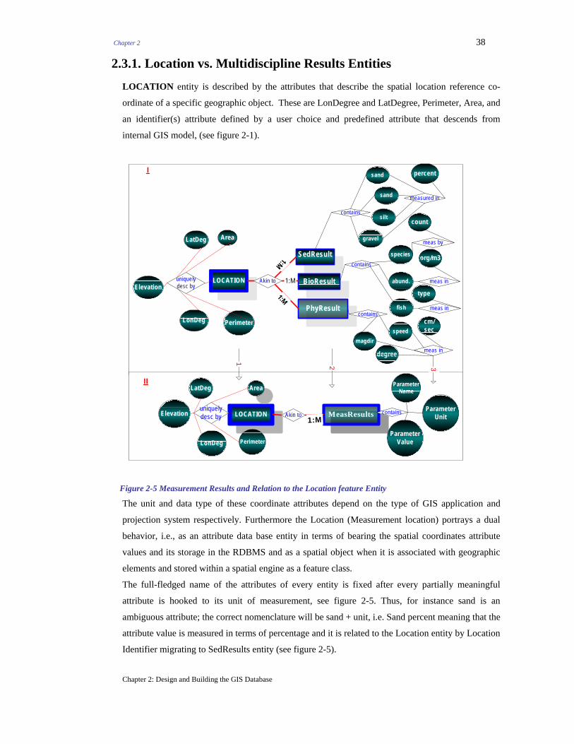
Chapter 2 38

2.3.1. Location vs. Multidiscipline Results Entities

LOCATION entity is described by the attributes that describe the spatial location reference co-

ordinate of a specific geographic object. These are LonDegree and LatDegree, Perimeter, Area, and

an identifier(s) attribute defined by a user choice and predefined attribute that descends from

internal GIS model, (see figure 2-1).

LOCATION

PhyResultcontains

meas in

speedcm/sec

magdir

degree

SedResult

contains

percent

measured insand

silt

gravel

sand

BioResult

contains

count

meas inabund.

species org/m3

fish

type

meas by

meas in

Akin to

1:M1:M

1:M

21

3

uniquelydesc by

Perimeter

Area

Elevation

I

II

LatDeg

LonDeg

MeasResults contains

ParameterName

ParameterUnit

ParameterValue

Akin to1:M

LOCATIONuniquelydesc by

Perimeter

AreaLatDeg

Elevation

LonDeg

Figure 2-5 Measurement Results and Relation to the Location feature Entity

The unit and data type of these coordinate attributes depend on the type of GIS application and

projection system respectively. Furthermore the Location (Measurement location) portrays a dual

behavior, i.e., as an attribute data base entity in terms of bearing the spatial coordinates attribute

values and its storage in the RDBMS and as a spatial object when it is associated with geographic

elements and stored within a spatial engine as a feature class.

The full-fledged name of the attributes of every entity is fixed after every partially meaningful

attribute is hooked to its unit of measurement, see figure 2-5. Thus, for instance sand is an

ambiguous attribute; the correct nomenclature will be sand + unit, i.e. Sand percent meaning that the

attribute value is measured in terms of percentage and it is related to the Location entity by Location

Identifier migrating to SedResults entity (see figure 2-5).


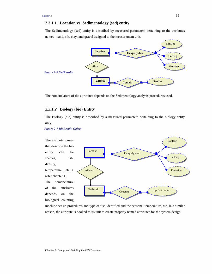
Chapter 2 39

2.3.1.1. Location vs. Sedimentology (sed) entity

The Sedimentology (sed) entity is described by measured parameters pertaining to the attributes

names - sand, silt, clay, and gravel assigned to the measurement unit.

SedResul Contain Sand%

Location

LonDeg

Uniquely desc LatDeg

Elevation Akint

Figure 2-6 SedResults

The nomenclature of the attributes depends on the Sedimentology analysis procedures used.

2.3.1.2. Biology (bio) Entity

The Biology (bio) entity is described by a measured parameters pertaining to the biology entity

only.

Figure 2-7 BioResult Object

The attribute names

that describe the bio

entity can be

species, fish,

density,

temperature... etc, +

refer chapter 1.

The nomenclature

of the attributes

depends on the

biological counting

machine set-up procedures and type of fish identified and the seasonal temperature, etc. In a similar

reason, the attribute is hooked to its unit to create properly named attributes for the system design.

BioResultContains Species Count

Location

LonDeg

Uniquely descLatDeg

Elevation Akin to


Chapter 2 40

2.3.1.3. The Physical Entity

The Physical (Phy) Entity is described by the measured parameters pertaining to the physical entity

only. The attribute names that reside within the physical entity can be current speed, current

direction, tides strength,

high tide and low tide and

others.

Figure 2-8 PhyResults

The nomenclature of the

attributes depends on the physical measurement set-up procedures. In a similar rationale, the

partially meaningful attribute name is fixed after it is hooked to its unit of measurement. Hence,

unambiguous nomenclature for current as current speed, and current direction are derived.

PhyResult Contains SpeedCm/Se

Location

LonDeg

Uniquely desc b LatDeg

Elevation Akin to

2.3.2. Cardinality Relationship

2.3.2.1. One to Many

In this case when we look for an attribute values belonging to Sedimentology entity, then we

make an instantaneous enquiry about which measured attribute value belongs to which feature class.

A Location ID (LocID) is a primary key field incorporated into an entity on level-2 (see figure 2-5)

creates a pointer to map and trace the information on that specific station, The relationship between

the Location entity and the other entities is termed as a one-to-many (1: M) see figure 2-5. Meaning

that there can be many measured attributes that can be geo-referenced uniquely by the spatial

feature pointer expressed relative to

a position. The de-normalized form

of the data model is depicted in

figure 2-5 (II), showing the product

of fusing entitles and related

attributes.

2.3.2.2. One to One:

Figure 2-9 Example of 2D Map indicating a bore hole ( BHs) Locations


Chapter 2 41

The relationship of one-to-one (1:1) can occur only when there is a correspondence between one

Location (LocID) and a specific record pertaining to a specific discipline and that record at single

borehole corresponds only to that location with LonDeg and LatDeg values.

For instance, the relationship of a Borehole entity and Location, see figure 2-9. This is true as long

as the relationship between the entities is

constrained to 1:1. However, in reality there is always database record represented by the Z value

inclined at a specific angle, then comes the representation transfer of the information from x,y (two

dimension feature) to a 3D (xyz) coordinate (see figure 2-10); which trespasses the uniqueness of

the records referenced by a unique spatial element. In such condition, the spatial information

retrieval would require an aggregating

tool.

Figure 2-10 Schematic Illustration of

a 3D Map

2.3.2.3. Many to Many

Many to Many: The many to many (M:

M) relationships exist if there is a

relationship in which many entity sets of

one entity are related to many entities sets in other entity. For instance:

A field can grow many types of crops,

Many types of crops can also grow in one field,

Many fault lines can shear the same Lithology (rock),

A single fault line with specific direction can shear many Lithologies (see figure 2-11).

Figure 2-11 A many to many relationship illustration

Although the data modeling technique ERD (entity relationship diagram) permits the specification of a many to

many relationships, these relationships are implemented in an object relational GIS database (see figure 2-12).

Because of such process, a many to many (M: M) relational model (see figure 2-12) uses a

connector feature table that contains a migrating mandatory identifiers of the M: M related entities


Chapter 2 42

to form a series of 1: M related tables. This would enable us to pinpoint Lithology records are

tectonically sheared by fault trends.

Similarly, the other entities (Field Data, Campaign Dates) and respective attributes describing any discipline

involved in the GIS data collection and measurement are derived in a similar process as indicated in Figure 2-

13.

LITHOLOGYuniquelydesc by

StrgNm

LatDeg

LonDegSheared by

LithDesc

Perimeter

Area

M M STRUCTUREuniquelydesc by

FtTrend

LatDeg

LonDeg

dip

Perimeter

Area

Strike

STRUCTUREuniquelydesc by

FtTrend

LatDeg

LonDeg

dip

Perimeter

Area

StrikeMAPS(connector)

CATEGORY MSLINK MAPNAME

LITHOLOGYuniquelydesc by

StrgNm

LatDeg

LonDeg

LithDesc

Perimeter

Area

Mapped in

1

Mapped in

1MM

Figure 2-12 Conversion of Relations cardinality

The Campdate data entity is the result of the combined product of all the field data dates of

measurement and sample collection during multidisciplinary GIS project activities.

Figure 2-13 Location vs. CampagindateData

This entity is populated by temporal attributes and related to a geo-referencing entity (see figure 2-13).

Location vs.

In a similar manner, the field data (see figure 2-14) entity is described mainly with attributes that

bear field descriptions on the site.

For instance, a Sedimentology scientist may describe his initial observation a muddy data collected

at the bottom of the water column as silty-clay type penetrated by roots and associated with benthic


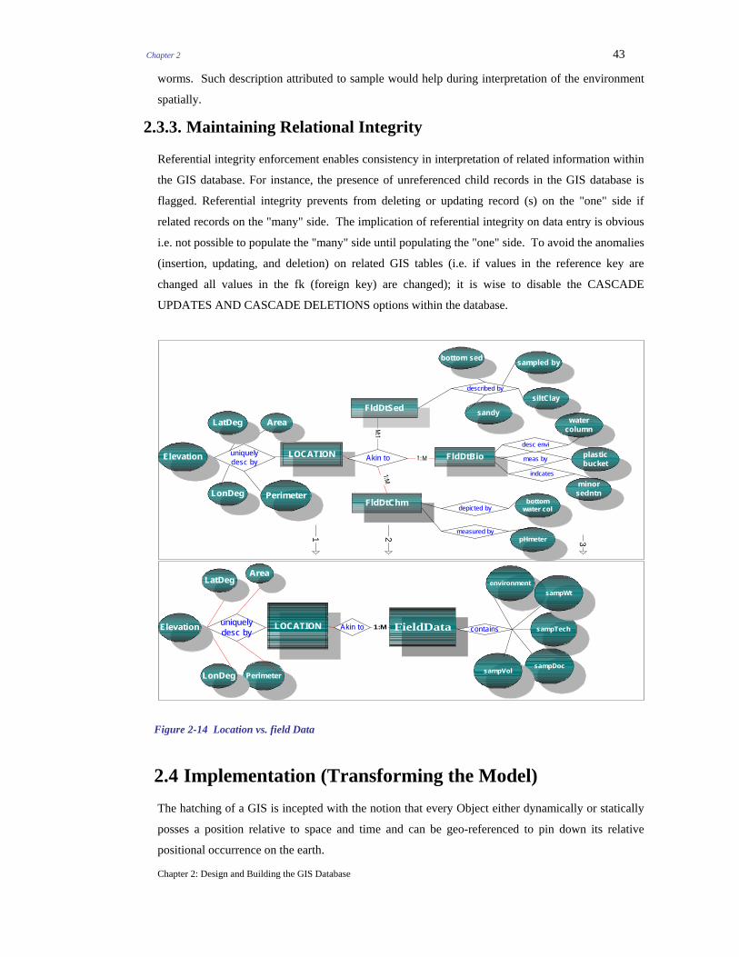
Chapter 2 43

worms. Such description attributed to sample would help during interpretation of the environment

spatially.

2.3.3. Maintaining Relational Integrity

Referential integrity enforcement enables consistency in interpretation of related information within

the GIS database. For instance, the presence of unreferenced child records in the GIS database is

flagged. Referential integrity prevents from deleting or updating record (s) on the "one" side if

related records on the "many" side. The implication of referential integrity on data entry is obvious

i.e. not possible to populate the "many" side until populating the "one" side. To avoid the anomalies

(insertion, updating, and deletion) on related GIS tables (i.e. if values in the reference key are

changed all values in the fk (foreign key) are changed); it is wise to disable the CASCADE

UPDATES AND CASCADE DELETIONS options within the database.

1 32

LOCATION

FldDtChm

FldDtSed

described by

FldDtBioAkin to

1:MM:1

uniquelydesc by

Perimeter

Area

Elevation

LatDeg

LonDeg

1:M

bottomwater col

pHmeter

siltClay

sandy

bottom sed

plasticbucket

watercolumn

minorsedntn

meas by

indcates

desc envi

measured by

depicted by

sampled by

1:MLOCATION Akin touniquelydesc by

Perimeter

Elevation

LatDeg

LonDeg

Area

FieldData contains

environment

sampTech

sampDocsampVol

sampWt

Figure 2-14 Location vs. field Data

2.4 Implementation (Transforming the Model) The hatching of a GIS is incepted with the notion that every Object either dynamically or statically

posses a position relative to space and time and can be geo-referenced to pin down its relative

positional occurrence on the earth.


Chapter 2 44

2.4.1. Spatial Entities

2.4.1.1. Object Composition

The attributes within the spatial feature table have been classified as - Informative attributes,

Identification attributes and Super Identification Attributes; where the Informative attributes

are fields that contain data items for informative purposes. The Identification attributes strictly

utilized as a basis for uniquely identify records, searching, sorting and joining two or more objects.

Super Identification Attributes: - are specific fields, which migrate as physical pointers from the

internal model to uniquely geo-reference associated GIS objects.

One can reference the Measurement Location object with one or more combined object identifiers.

However, a single attribute entity, which uniquely identifies the database record akin to different

fields but to the same entity, is required.

Close inspection of table 2-2 indicates that the station (LOCID) attribute is a key at the relational

linkage level; however, this is true as long as it stays unique. An ObjID is an attribute defined to

bridge the gap between the internal and external systems entities, spatially join, and retrieve

referenced information.

2.4.1.2. Object Identifier

The presence of the elevation attribute within the LOCATION entity raises the problem of

ambiguous records, which could stem out during sampling or measurement in a single location. At

this point, the station (LOCID) attribute loses its constraining power and could not identify spatial

information uniquely. However, it is possible to generate different object layers with respect to the

Z values. Therefore, the ObjID and MAPID (Geographic and MGE, ObjID ArcView) identification

attributes takes over the system integrity, functionality, i.e., by creating a pointer over a pointer as

indicated below.

A Spatial Record: -

2.4.1.3. Point Object: Measurement Location

The location entity is described by coordinate attributes and one or more internal mandatory pointer.

Upon geodetic referencing the LOCATION, entity is used as the primary entity. In real world

representation, the attributes of the location entity represent geographic point object. Depending on

the data items and required visualization the real world object can be represented by a two-

dimensional point, compose of latitude and longitude or a three-dimensional point, see table 2-2.


Chapter 2 45

Table 2-2 A double Pointer objects

The dual pointer data structure (table 2-2) depicts two important records. The first row with all

possible spatial attributes, second row depict attributes before being associated to the spatial

features. The different representation of latitude and longitude, (see table 2-2), (Londec and Lontxt)

is to facilitate populating the geodatabase and generating objects in different GIS applications. The

presence of elevation indicates the type of the seed file or template for a 3D GIS map.

A 2-dimensionl GIS contains mandatory coordinate attributes implies that the spatial relationship

visualization is to be implemented on a 2-dimension map. On the other-hand a 3-dimension contains

3 mandatory coordinate attributes and implies that the GIS’ object retrieval will include a third

column of elevation to geo-reference, and visualization is implemented on a 3-dimension

perspective. The fact that third dimension visualization in a GIS environment poses a problem can

be resolved by a vertical scale modification.

2.4.1.4. Polygon objects: Estuary morphology and Zone

Spatially, the Estuary object contains measurement locations. The relationship between the Estuary

object and location is 1: M. spatially the measurement locations are within the Estuary.

Zone: Polygon object

2.4.1.5. GeoLithology and GeoTectonics: Polygon and Polyline Objects

GeoLithology: The Lithology object is described by informative attribute such as the lihological

composition, rock types, lithologic contacts (boundary lines), stratigraphic name and geo-

referencing coordinate attributes. The area and perimeter attributes depicts zone of influence of each

rock composition distribution.

GeoTectonic Structure: GeoTectonic Structure entity is described with tectonic fault lineaments.

This include the fault direction, dip and strike) along the shear zone. The Results Table was also

structured in the same manner to describe and disclose the different relevant attributes.


Chapter 2 46

2.4.2. Relationally Structured Entities (RSE)

The Field Data, Campaign data, Disciplines and Results are the relationally structured entities

controlled mainly by their own attribute database identifiers. However, they can be geo-referenced

via migrating objecteID and related discipline name to generate any spatial object, See figure 2-15.

Figure 2-15 Relational structure of UDE Chapter 2: Design and Building the GIS Database

Chapter 2 47

2.4.3. GeoDatabase Cardinality Relationship

Table 2-3 GIS Database Cardinality Relationship

2.4.4. Physical Structure

2.4.4.1. Schema Data Definition

The relatively higher-level representation of the database is defined as a schema or conceptual

model. The database tool used to define the conceptual schema is a data definition language or

DDL. At the physical level, the data items are defined in terms of parameters such as the number of

bytes of storage they occupy and the address at which they are to be found in a physical memory.

The physical creation of the entities and the attributes leads to the building of the GeoRelational

GIS Database.


Chapter 2 48

The physical definition encompasses –

(a) DDL or DAO for the aspatial, (b) Spatial interface functions for geographic elements and for the

Meta data object. The considerations pertaining to (a) and (b) include -

Field types

Storage space

Operations anticipated on the attribute

Calculation (numbers OR currencies) not texts or OLE.

OLE Object fields for metadata

Decide if temporal query sorting (use date/time formats)

2.4.5. (DDL) The data definition language

In a dual architecture GIS, the definition of an ODBC enables database creation and facilitates the

creation of a new GIS project connectivity and workspace. The workspace is populated by the

system and user defined objects. Thus, establishing Open Data Base connectivity (ODBC) is

mandatory to link the external and internal systems (details see chapter 3).

The definition of the attributes data types can be specified in the table design view, query parameter

dialog, in visual basic, and in SQL view or within the spatial engine interface.

SQL (structured query language) is an access and manipulation language; it is acknowledged as the

relational database language, [60]. SQL is a non-procedural, i.e., one need to tell the computer what

data is interested to process and view. With SQL, system design specialist, application developers

and end users can work together to

perform smooth interaction of the

application requirements.

Figure 2-16 Location GeoTable

Out of the many data types, only

numeric, textual (char) and date/time

data types are defined applying non-

procedural SQL’s DDL. Otherwise,

data such as images, points, lines and shapes can be defined using special graphic programs.

However, the procedural method is more secured from the database integrity and security

perspective but it requires a database programming knowledge. Both methods were used during the

physical design and implementation of the geodatabase, see figure 2-16.

The DDL components of SQL (specific to Access) include:

CREATE, ALTER, and DROP.

The CREATE command syntax.


Chapter 2 49

CREATE TABLE name

(ColumnDefintion), [Multicolumn - Constraint]) [Single-constraint]

ColumnDefintion is column name, followed by a data type (with size if appropriate), and followed

by a single column constraint.

Figure 2-16 illustrates the definition of the master table location using the DDL. The MSLINK is a Primary

key. It is designed to be an object ID of the feature class table (object). The MAPID is specific to MicroStation

Geographics. It is required for spatial connection between the map and database records. The LatDeg and

LonDeg are coordinates in different formats.

Area and perimeter are specific for polygons but

are incorporated with alternatives formats and

the Easting and Northing are coordinates in map

units.

Figure 2-16 CampDate GeoTable

In the Campdate table, the MSLINK

(definition of CampDate) is a migrated key from the location feature class whereas the temporal

data were collected. The MAPID and station have the same context as the description of table

location. The samp_date, samp_time, samp_time_e, and samp_time_St are the temporal parameters

(see figure 2-17).

Figure 2-18: Results GeoTable

The temporal attributes pertaining to

table CampDateData references the

feature table LOCATION so that

spatial information retrieval can also

be interpreted with respect to

temporal aspects.

The definition of Measurement Result table is described by multidisciplinary attributes. All the other tables

are made to indicate the pointers towards this table. Thus, all the marine information stored in the other

tables can also be reference.

2.4.5.1. Indexing Tables (non procedural)

CREATE INDEX command is described by the following syntax.

Create [unique] index Name

On TabName ([Colname) [asc/desc)


Chapter 2 50

[With (primary) ~disallow null or ignore null)]

Where the ASC and DESC stands for ascending and descending

Illustrating the creation of GeoRelational indices:

Create Unique Index LocationIndex on Location (Mslink, Station, and Asc) With Primary;

Create Unique Index Fielddataidx on FieldData (Field_Code) With Primary;

Create Unique Index Resultsidx on Results Meas_No) With Primary;

Indexing can be executed on a single column or in concatenated columns. Indexing an elected

field(s) in a table is quite important for speeding up access and queries on the indexed fields, sorting

and grouping operations. See appendix A, for the full-fledged geodatabase structured data

definitions.

2.4.5.2. Enforcing Index and Uniqueness

Enforcing Index and Uniqueness is applied to guarantee that a column or combination columns is unique

for every row in the table. A UNIQUE key word is used to enforce the information integrity. Indexing a

mandatory spatial pointer enhances the retrieval process in general but may slow the updating.

Searching spatially geo-referenced records, either for tabular display or thematical visualization

based on the attribute values associated with the geographic objects is better done by creating an

index on the ObjID with Primary key restriction. Furthermore, besides the SQL DDL indexing

procedure, DAO (Data Access Object) was implemented to index the specific mandatory field of the

GIS tables (figure 2-19).

Figure 2-17 : Enforcing an Index Example, the following procedure creates an index on the Location Object mandatory ObjID known

in this cases study as MSLINK. The dimension database is defined and is set to the database which

is being active and is opened by the set dbs = OpenDatabase ("guayas.mdb"). This is followed by

the db.execute to create the index with primary, ignore null, or unique…. In order to perform the

indexing on all the selected tables, the procedures are called from a single command button

interfaced within the attributed database.

2.4.5.3. Enforcing Referential Integrity

The Relation object provides information to the underlying database engine about the relationship

between fields in two entities [34]. For instance, the relation object implements the referential

integrity between the LOCATION and MAPS objects as follows.


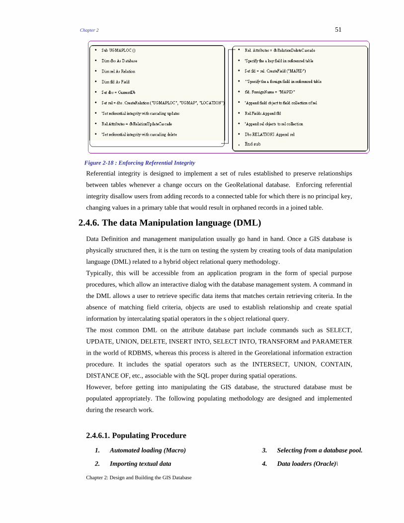
Chapter 2 51

Figure 2-18 : Enforcing Referential Integrity Referential integrity is designed to implement a set of rules established to preserve relationships

between tables whenever a change occurs on the GeoRelational database. Enforcing referential

integrity disallow users from adding records to a connected table for which there is no principal key,

changing values in a primary table that would result in orphaned records in a joined table.

2.4.6. The data Manipulation language (DML)

Data Definition and management manipulation usually go hand in hand. Once a GIS database is

physically structured then, it is the turn on testing the system by creating tools of data manipulation

language (DML) related to a hybrid object relational query methodology.

Typically, this will be accessible from an application program in the form of special purpose

procedures, which allow an interactive dialog with the database management system. A command in

the DML allows a user to retrieve specific data items that matches certain retrieving criteria. In the

absence of matching field criteria, objects are used to establish relationship and create spatial

information by intercalating spatial operators in the s object relational query.

The most common DML on the attribute database part include commands such as SELECT,

UPDATE, UNION, DELETE, INSERT INTO, SELECT INTO, TRANSFORM and PARAMETER

in the world of RDBMS, whereas this process is altered in the Georelational information extraction

procedure. It includes the spatial operators such as the INTERSECT, UNION, CONTAIN,

DISTANCE OF, etc., associable with the SQL proper during spatial operations.

However, before getting into manipulating the GIS database, the structured database must be

populated appropriately. The following populating methodology are designed and implemented

during the research work.

2.4.6.1. Populating Procedure

1. Automated loading (Macro)

2. Importing textual data

3. Selecting from a database pool.

4. Data loaders (Oracle)\


Chapter 2 52

1) Automated loading (Macro)

a. An action macro defined to

import textual data (Spreadsheet)

b. Action: Transfer Spreadsheet

c. Transfer type: >Import

d. Spreadsheet type:> format or

application

e. Structured table name: Location

f. File name: drive:\x\x1

g. Field names (y/n):> yes

Figure 2-21Populating Process

The steps applied to achieve figure 2-16 are -

Formatting raw data or retrieving from a structured geodatabase

Establishing a populating program

Spatial function to manipulate the spatial objects

Accordingly, the data in a remote location (flat file or geodatabase) is populated into the target table

at any time by clicking a loading command button attached to an interfaced macro.

2. Importing textual data

The importing of external data is rather specific to a database wizard application. The external data

could be directly imported into the database or linked. However, linking will not allow the database

to be modified.

3. Selecting from a database pool: Query Database data pool

Syntax

Insert into A (a1, a2, a3…) (a1…an are attributes of A)

Select (b1, b2, b3.) from B (b1…bn attributes of B)

Where A.Id (all possible operators);


53

The above syntax indicates data extraction possibility from a source table (TbB) to an empty structure table

(TbA). For instance, it is possible to create different structured tables from a single table that contain

completely heterogeneous attributes information together.

2.4.6.2 Select Statement

The SELECT statement is the workhorse of the SQL commands.

It can return a table and perform the relational algebra SELECTION and PROJECTION.

SELECT: denotes the relational algebra operation of Projection and the WHERE performs the

Selection. The predicate indicates the handling of the duplicate return rows.

ALL: (distinct, distinctrow) return the entire column description and the distinctrow return unique

records not unique value. Therefore, if we have attribute name named as station with data item in 1, in

ten records the distinctrow returns all the ten unique records with data item 1 record. To avoid the

duplicate value the three characters of the Key word (DISTINCTROW) are removed and returns unique

values.

FROM TblExpression: The FROM clause specifies the tables or queries from which the SELECT

statement is to take its rows. The TblExpression can be a single or more tables separated by commas

or joins.

WHERE Row Condition: any expression such as the attribute names, constants, arithmetic expression

such as (>, =…. BETWEEN) and logical (AND, or, XOR, not as well as functions and relations) e.g.,

LIKE, min (attribute name)…etc.

GROUPBY CRITERIA: The group by criteria allows records to be grouped together for computing

the value of an aggregate function, (Avg, count, min, max... etc), (see figure 2-23a).For instance, the

group by function is very important, especially to

relate the spatial table or associated table with RSE. It

returns results corresponding to the spatial entity. The

result retrieved can be spatial and thematically

visualized in an associated feature table.

HAVING Group Criteria: - The having option is used in

conjunction with group by option. It allows the query to

specify criteria in terms of aggregate functions for deciding

which data to display. It is shown that the

Figure 2-22 The SELECT and UPDATE


54

WHERE clause restricts the number of attributes or columns that participate in the grouping, and

hence contribute to the value of the aggregate functions, whereas the HAVING clause affects only

the attribute values to be displayed. ORDER BY option sets the default sort order of the database records.

Likewise, spatial operators are applied on spatial operations to retrieve and perform spatial analysis using

the spatial operating tools.

2.4.6.3 Updating Database

An updateable Table enables us to change and edit the content of the GIS database and any change

is reflected on the underlying GIS tables. Updating is important especially when the GIS databases

develop through time and a change is required (see figure 2-23b.

The possibilities of updateable tables depend on the conceptual relationship of the entities and the

possible definition of enable cascade update. If the query is mainly based on a single table or, in a

one to one relationship then there is less difficulty compared to a one-to-many relationship. The

Cascade Update Related Fields must be updated to execute the changes.

2.5 Results and Conclusions Designing an endurable and flexible Geodatabase system requires conceptual structuring of the

geodata model. This depends on the extent of understanding clearly a targeted problem and time

allocated to perform a sequence of Design and Implementation tests; this process has been done

during the conceptual and physical design of the geodatabase model.

The Construction and Integration of the coastal zone Multidisciplinary Geo-Relational data model

have been founded on object relational and the conceptual entities were represented using

information structure diagrams (ISD).

Data Definition Language was applied to the physical GIS database creation and implementation.

The objects-pointers have been hooked to the relationally structured entities (RSE) to achieve the

assimilation of geographic objects with attribute database records.

Amalgamating process has been implemented to avoid redundant Measurement Result entities

belonging to different disciplines. This has been achieved by de-normalizing the normalized

entities. The principle facilitated the mechanism of interacting objects and performs spatial analysis

at the phase of spatial information mining.


Chapter 3 55

Chapter 3: Building the Spatial Database

3.1 Introduction Design of a GIS project can be done with little hindrance if there is a fair understanding of what the

specific GIS project is comprises of and how it should be structured. Grasping this notion serves as bases

for creating a powerful spatial database development environment for management, analyses and

visualization geographic information system.

3.2 GIS Data Flow Globally, the construction of Geographic Information System is based on two types of data, coined as Non

Spatial (Aspatial) and Spatial (see Figure 3-1, I and II). Aspatial data are the characteristics that describe

the spatial

elements. Spatial

data are any

information

about the

location and

shape of, and

relationships

among

geographic

features [25].

The non-spatial

data are attribute

data source for

the data model

and are

structured and

created before

being integrated

with the spatial

objects in a dual

object relational

system.

Figure 3- 1 Building GIS data flow diagram

Chapter 3 56

Otherwise, the spatial data can be of raster (scanned paper or remote sensing image) or vector origin. One

mandatory process required during the building of the spatial database is registration of the maps or

assemblage of features with an appropriate projection system relevant to the specific area.

During scanning process, the data is stored as pixels form, which divides the imaged into regular grid

structure of rows and columns. Each cell within this matrix contains an attribute value as well as location

co-ordinates. Vector features are those geographic elements, which can be generated by tracing an image.

Vector features are comprised of points, lines and polygons. All lines have a beginning and ending points

(vertices). Space required by vector elements is less than that of raster. Once a feature is stored in the

system, then anything outside is non-existing space.

Referring to figure 3-1,vectorised data require a visual inspection (step 2-1) to identify areas of interest and

target features. The data generated in step 2 and visualized in step 2-1 are subjected into topology clean up

processes (step 3), specially in the aftermath of digitizing, where so many undesired line fragments, line

offshoots and gaps…etc., are produced, (see figure 3-1, steps3-1 to 3-4). Once laborious process of

topology operation is accomplished, then the geometric elements are processed to produce associated

geographic features, using appropriated spatial tools or spatial functions.

For instance the spatial function: - Place Point (X1, Y1) Values (_, _) creates a point by providing the

coordinates. Likewise, the attaché spatial function would prompt geographic object to be attached with

database record. Also a point feature table can be updated to create a line feature as follows- Update

MYpointtable set Obj = createline (StartX, StartY, EndX, EndY)

The object building coordinates are stored within a feature table (see figure 3-1, step 4). Feature tables are

distinguished from attribute tables in that the feature table represent object and object identifiers (see figure

3-1, step 4-1). Once step 4-1 is accomplished, the process of spatial and aspatial integration can be

executed provided the geodatabase structuring process (data modeling) is completed. If not then step 5;

process of data model (attribute data) is completed by executing (see figure 3-1, steps 5-1 and 5-2), which

are based on constraints established using information structure diagrams and physical creation of the

attributes within the database.

Note: A quick creation of GIS can be achieved by populating georeferencing-bearing data (see figure 3-1,

step 5-4 and 5-5) utilizing the integration process (see figure 3-1, step 6, 6-1). However, a stable and well-

organized GIS involves the populating of the data (see figure 3-1, step 5-3) to the data source or database

(see figure 3-1, 5-2) then after, step up the integration (see figure 3-1, 6, (6-1) of linking and association of

the database to spatial elements.

The procedures of integrating (step I) and (step II), using (see figure 3-1, step 6-1) encompass the

application of a spatial interface and spatial analysis tools. Results of the integration are expressed

thematically and visualized spatially. The eventual output is employed in a crucial decision-making about

the issue being explored (see figure 3-1, step 7)

Chapter 3 57

3.2.1 Feature set up building Components

Spreading the multiple features pertaining to a single Category, for instance as implemented in this PhD

research work, defined as the Marine Map or Geology over many levels is quite important for the spatial

data management pre to the feature set up, defining features, category specification, assigning symbology

to geographic object type is a essential.

Figure 3-2 depicts a typical data flow diagram of the GIS feature setup.

Figure 3- 2 Feature set up data flow

Referring to figure 3-2: -

(Figure 3-2, 1): - The Category is described by its own properties of the seed file type (map), its index,

extension of the map to be generated. The different extensions related to the Category are used to distinctly

differentiate maps in the GIS (as dgn, tab)…etc). The overlap is exploited for the possibility of importing

other GIS projects to the existing GIS system and the level indicates the position of the category as distinct

from the pertinent features.

(Figure 3-2, 2): - The assignment of the textual description and symbology is used to distinguish the

feature types by their respective properties. The element and thematic type represent the objects to be

attached spatially and the bounding elements.

(Figure 3-2, 3): - displays properties of the features, for instance, a point of centroid type can be

associated to its boundary to generate a spatial extension of the associated database records.

Chapter 3 58

(Figure 3-2, 4): - Different features can be distinguished by level, style, and color and feature command.

Duplicate records are controlled by linkage type and the read/write type is specified with respect to the

feature class table. The whole components defined in the hierarchical data flow diagram are properties of

the special working system files, which are designed to be associated with spatial data source of the user

and store the main tables that directly engaged with the spatial analysis and management of the spatial

information.

3.3 GISs project structures Different GIS applications have different structures. As an example1, the GIS project of MicroStation

Geographics [11] is composed of Mscatalog, category, feature, maps and feature-command (SGEs) (see

figure 3.2). Spatial and aspatial attributes creation and a linkage are committed within the project. As an

example2, In an ArcView GIS (3.2a) [21], a project contains all the view, tables, charts, and layouts and

scripts that used for a particular project work. A view defines the geographic data that will be used for

spatial analysis. The step-by-step process of building GIS project is explained bellow.

Figure 3- 3 Project specific to MicroStation Geographic and MGE GISs

3.3.1 The Spatial Components Work Space

3.3.1.1 Spatial components

Category: - is an assemblage of related features and is distinguished by specific extensions. For instance,

the Marine maps category described by a map extension of the .MAR. The Mar.Estaury.centroid is feature

description belonging to that category (see table 3-1).

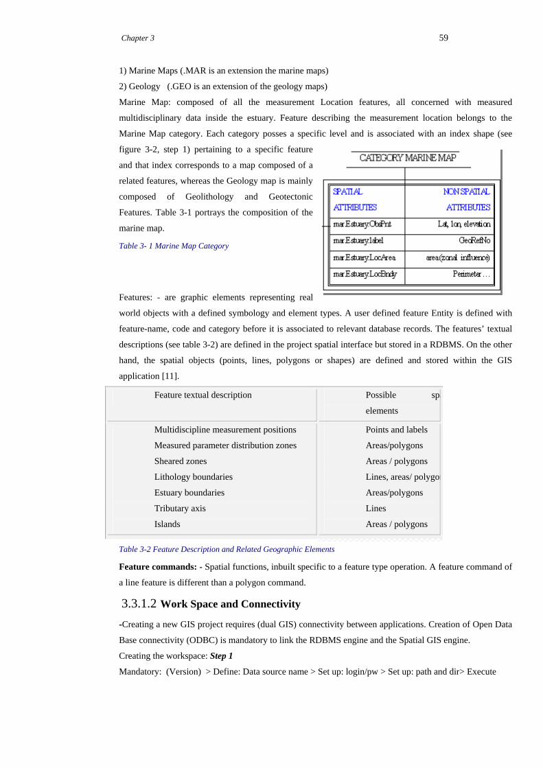
Chapter 3 59

1) Marine Maps (.MAR is an extension the marine maps)

2) Geology (.GEO is an extension of the geology maps)

Marine Map: composed of all the measurement Location features, all concerned with measured

multidisciplinary data inside the estuary. Feature describing the measurement location belongs to the

Marine Map category. Each category posses a specific level and is associated with an index shape (see

figure 3-2, step 1) pertaining to a specific feature

and that index corresponds to a map composed of a

related features, whereas the Geology map is mainly

composed of Geolithology and Geotectonic

Features. Table 3-1 portrays the composition of the

marine map.

Table 3- 1 Marine Map Category

Features: - are graphic elements representing real

world objects with a defined symbology and element types. A user defined feature Entity is defined with

feature-name, code and category before it is associated to relevant database records. The features’ textual

descriptions (see table 3-2) are defined in the project spatial interface but stored in a RDBMS. On the other

hand, the spatial objects (points, lines, polygons or shapes) are defined and stored within the GIS

application [11].

Feature textual description Possible spa

elements

Multidiscipline measurement positions

Measured parameter distribution zones

Sheared zones

Lithology boundaries

Estuary boundaries

Tributary axis

Islands

Points and labels

Areas/polygons

Areas / polygons

Lines, areas/ polygon

Areas/polygons

Lines

Areas / polygons

Table 3-2 Feature Description and Related Geographic Elements

Feature commands: - Spatial functions, inbuilt specific to a feature type operation. A feature command of

a line feature is different than a polygon command.

3.3.1.2 Work Space and Connectivity -Creating a new GIS project requires (dual GIS) connectivity between applications. Creation of Open Data

Base connectivity (ODBC) is mandatory to link the RDBMS engine and the Spatial GIS engine.

Creating the workspace: Step 1

Mandatory: (Version) > Define: Data source name > Set up: login/pw > Set up: path and dir> Execute

Chapter 3 60

New empty geodatabase (personal geodatabase) workspace created (see figure 3-4).

Figure 3-4 ODBC

Specification

The workspace is populated by the system (GIS geographic, MGE and user defined tables. In the Case of

the ArcView GIS, only the user-defined tables (UDEs)

are stored in the database. SQL connect is used to link to

the spatial engine (ArcView).

GIS Features Generation: Step 2

Figure 3-5 Project Setup (MicroStation Geographics)

Eventually the system tables generated from within the

GIS application are populated in the geodatabase

workspace (see figure 3-6). From then on, they are

available to be processed spatially in any GeoRelational

GIS environment.

Figure 3-6 Populated Geodatabase work space

3.3.2

3.3.3 Features definition

Definition and implementation of the feature elements or geographic objects attributed to the user-defined

feature entities is carried out in the feature set up interface. It is equipped with push button tools [Insert,

Chapter 3 61

Update, Delete Commit, and Rollback] and list box, which enable define categories, features and feature

commands [1].

Insert - Key-in: FOCUS INSERT create a new category, feature, or command by adding a new row to the

specified database table and populating the new row with data determined by user selections in the settings

box.

A macro tool, MicroStation basic extension program is used to generate the category, type of file, map

extension and level of the category (see figure 3-7). More over the FOCUS UPDATE, focus DELETE and

COMMIT and ROLLBACK are applied to update, commit and undo feature operations respectively.

Figure 3-7 Generating the Marine Map Categories and related features

Referring to figure 3-8, the populating of the category and related features is described as follow: -

Name>> the name of the selected category.

Extension>> the category name's extension. (3 letters)

Index >> the name of the category's index file

Level>> The MicroStation level that contains the index shapes.

Level used by the active category) highlighted.

Allow Foreign>> If on, permits the selected category to contain features belonging to other categories.

Overlaps>> Indicates that the index polygons for maps in the category may overlap.

Chapter 3 62

Figure 3-8 Categories and Features Definitions (Geographic GIS)

3.3.3.1 An Active Feature

The purpose of feature definition is critical since it is at this phase that the GIS features are decisively

defined and implemented. Any structured database record of the project is to be associated with these

spatial elements. A feature represents

an object. It has its own descriptive

symbology and usually contains

descriptive information. Category

Marine Map is triggered and its

attributes are defined in space provided

as features (see figure 3-9)

Figure 3-9 An active Category and Related

Features

An active feature can be displayed for

association process by triggering the

category list. Selecting one of these will populate the Feature list box with the features pertaining to the

category, see figure 3-9.

Chapter 3 63

The textual features describe the Geographic objects, which would be linked to geometric objects. These

Geographic objects references could be shapes, ellipsoid, point’s lines and also texts.

SPATIAL

FEATURES

NON SPATIAL

ATTRIBUTES

geo.Lithology.centroid Lat, lon

geo.Lithology.label StationCode

geo.Lithology.area area

geo.Lithology.boundar Perimeter …

SPATIAL

FEATURES

NON SPATIAL

ATTRIBUTES

geo.Stru.point Lat, lon

geo.Stru.label GeoRefNo

geo.Stru.ShearedArea area

geo.Struc.ShearedZone Perimeter …

CATEGORY GEOLOGY

SPATIAL

ATTRIBUTES

NON SPATIAL

ATTRIBUTES

mar.Location.point Lat, lon, elevation

mar.Location.label StationCode

mar.Location.area area (zonal influence)

mar.Location.line Perimeter …

SPATIAL

ATTRIBUTES

NON SPATIAL

ATTRIBUTES

mar.Estuary.ObsPnt Lat, lon, elevation

mar.Estuary.label GeoRefNo

mar.Estuary.LocArea area (zonal influence)

mar.Estuary.LocBndy Perimeter …

CATEGORY MARINE MAP

Table 3-3 The Coastal Periphery and Main Estuary feature descriptions

3.3.3.2 The spatial Features’ methods and properties

1) Element Type - the real world object feature e.g., LString, line, shape…etc.

2) Thematic Type- describes the spatial features visualization

3) Element strength- associability with related feature types

The steps (1-3) are crucial for later feature translations and interoperability among GIS applications (see

chapter 6).

3.3.3.3 Element Type Validation

Setting to Interest - enables the designated Category-feature to be attached to any element

Setting to Similar- enables the designated feature to be attached to the option shown on Element Type

Setting to exact - enables the designated feature to be attached only to the element type option shown on

Element Type. This is the same as defining an attribute as integer data type but trying to insert a non-

integer value. That is what is termed as data validation rules. Defining clearly the feature type at this level

facilitates the thematic resymbolisation.

Chapter 3 64

Theme Type- identifies a feature's topological type.

Point Feature - identifies the feature as a point.

Line Feature - identifies the feature as a linear element.

Text Feature - identifies the feature as a text element. Used only when element type is set to a text.

Setting boundary: Boundary - identifies the feature as a linear element, implying that such features will

obey topological rules

Setting Centroid - identifies the feature as a topological centroid. The associated element type can be a

cell, point, or text type. The centroid feature is to be linked or joined to a unique database row whose

attributes apply to the surrounding topological area.

Setting Label Features - text elements linked to a database row.

Display order: - Feature tags with low number display first than those with high number. Higher

numbered features display on top of lower numbered. Hence, layers of maps can be visualized according

to the defined order number. Fence Sort Display keyed in can display features in a sorted order during a

thematic display operation.

Feature Table: - Feature table with database records identifiable by featureID Linked to Centroid where

the centroid is associated to the area boundary feature. This object is also composed of all the possible

categories and related feature descriptions describe every geometric object during any process of spatial

analysis. The feature table is characterized by the each feature code that applied to distinctly identify any

object and associate information. The feature codes are related spatially to the respective categories.

Referring table 3-4, the category (feature table location) is related to the feature codes – 3, 3.1, 3.2, 3.3,

referring to the Mar.Marine.Line, Mar.Amrine.Point, Mar.Marine.Area and Mar.Marine.No. Furthermore,

the feature type, feature level, feature color and feature weight are the symbology of every geographic

element described by the respective feature table.

The feature length, feature weight and tolerance are defined to a specific feature type. The location feature

table represents, multiple disciplinary measurement location and is point a feature type. On the other hand

the Lithology and tectonics feature table with information related to the coastal or periphery of the main

estuary.

The sed feature table is one of the measured result feature tables for sediments. On the left side of the table,

3-4 is an attribute named MSLINK. This is a unique feature identifier is generally generated by the spatial

application during feature creation.

Chapter 3 65

Table 3-4 GIS building Categories and Textual Features description

Ugcommand_table: - each defined feature is associated to a specific feature command name and a

command key in. For instance, the AUTO COMMAND for the features mar.Location.Point and

mar.Location.Label is PLACE POINT and PLACE TEXT respectively, see Table 3-5A.

Table 3-5 (A) Feature Command (B) Maps table

Chapter 3 66

The feature value is related to the Mslink of the features table (see table 3-4). This process of allows us to

assign every feature a geometric indexing key i.e. the MSLINK. MSCATALOG TABLE: The GIS

application requires a data dictionary table that stores and references all GIS building block entities.

Table 3-6 Mscatalog table and Ugtable-cat

Mscatalog: - Is composed of two mandatory attributes (Tablename and entitynum) while it generates

automatically during the project creation. It is mandatory system table used to store in system tables.

Implicitly, any table that is not incorporated in the Mscatalog could not be recognized by MicroStation

geographic specific. The Ug_Table_Cat: - It is use to store the names of the objects associated to the GIS

project and the spatial pointers that implement the linkage of attribute and graphic elements.

3.3.4 Integrating the GIS Entities

3.3.4.1 Interoperability

The definition of the features in feature setup interface, utilizing feature transactions tools generates an

exportable file (.EXP). The .EXP contains all the information stored in the GIS Project geodatabase. This

extension is utilized to perform two types of linkages.

Perform feature description vs. spatial element linkage and (B)-Perform spatial elements (accomplished in

A) vs. structured database records association. The first process enables us to label and identify any

geographic object.

The second linkage is used to assimilate certain structured tabular information with the geographic

elements by means of spatial functions (for instance the attach or detach function).

From the on, the associated object information can be spatially retrieved by utilising the object identifier

(MSLINK), which is associated to every feature type and specific feature code. At this phase of the

constructed Georelational GIS project can be communicated with other GIS applications, as indicated in

figure 3-10 based on the object relational structure unveiled in figure 3-11.

The objects (features) are related to the system tables by two fields, MSLINK and MAPID (Geog. GIS)

feature ID (ArcView and ArcGIS) and MapInfo_ID (MapInfo GIS).

Chapter 3 67

two way spatialinfo transfer

two way spatial infotransfer with conversion

process

Connection Spatial vsRDBMS engines; PossibleSpatial info processesing

ODBCENABLED

GISDATABASE

ArcView

Geog/MGE

MapInfo

connection anddata transfer

GeoRelationalData Model(SGE

& UDE)

ArcGIS

Figure 3-10 Possible communications among GIS applications projects

Three possibility of interoperability indicated (a) a two way spatial information transfer without loss of the

spatial objects properties; for instance the preservation of shape and projection.

This process is executable among open GIS complaint applications and by means of feature translating

applications. The connection between Georelational data model and spatial engines is achieved by means

of application interfaces, which are composed of data transfer DLLs. This includes ODBC and ADO as

experimented in this research work.

3.3.4.2 The Related GeoDatabase System

The Geodatabase model (see figure 3-11) is composed of (a) System generated entities - block 1, (b)

Estuary environment entities, - block 2, (c) Coastal periphery Entities, - block 3 and relationally structured

entities, which are hooked to the master, feature tables (objects). Both blocks (2 and 3) are connected to

the system-generated entity via maps entity to complete the transfer of the information with the system.

Maps entity is an entity that is described by attributes map-name, category and MSLINK. MSLINK is a

migrating pointer from category entity in a 1: M relationships, likewise, the same information flow holds

true for the category vs. feature tables (see figure 3-11).

Chapter 3 68

Figure 3-11 Integrated GIS Database

The Location feature table is referenced to the maps system table by a common field; similarly, the

Estuary,

Tectonic structure and the Geology Feature tables are hooked to the maps entity to create a path of spatial

information flow. The feature table (object) and system-generated tables are stored within the Mscatalog

Table (block 1) so that spatial process is executed successfully. The system linkage zone is performed

between the user defined and associated feature table. For instance the location, lithology … etc., and the

system maps table is related to the category and the category to the feature table. All are encompassed

within the Mscatalog.

Chapter 3 69

3.4 Results and Conclusions The process of spatial database building requires a series of conceptual, as well as practical

experimentation. It requires piecing together of a data model, system entities and application tools,

identifying features, connectivity among the spatial and aspatial data and fundamental know-how of

the GIS objects during spatial operation phase of the GeoRelational GIS.

The methodology of enacting varies from one spatial engine to the other; however, one common point

that all GIS construction process requires construction of the GIS project where all the GIS building

block entities are integrated by means of associating geometric objects to structured tabular

information. These processes have been accomplished to achieve the full-fledged GIS project system.

To implement its applicability, the Geodatabase model has been tested across different GIS

applications. The connectivity of the attribute data model and the different spatial engines has been

established by means of ODBC and ADO during the GIS project operational processes.

To achieve a smooth interoperability, elected migrating spatial pointers and the relationship among the

objects have been established, the seed file that generates different features type and dimensions have

been defined appropriately.

Chapter 4 70

Chapter 4: Spatial Database Structure

4.1 Introduction An important subject matter of this chapter is spatial database structure construction. To begin with,

first, an introduction will be given about the basic database models (Hierarchical, Network, and

Relational) and will be ensued with more emphasis on the object-relational model, which is suitable

for dealing with multidisciplinary spatial problems. Further, the importance of avoiding redundancy

of spatial features and topological relationship (line, plotline and Polygon-Coordinate-Attributes) are

discussed. Eventually, the processes of binding geographic objects are explained, using illustrative

object relational methodology.

As a departure point, a single map composed of polygons, lines and points is provided. The common

line boundary between polygons and vertices that connects the lines derive the relationship among the

polygons. The practic1ality of this data structure is elaborated (see Figure 4 -1) and onward.

Figure 4- 1 An Illustrating Map

Object’s Relationship:

1. Silt Clay is a map

2. Polygon I is_part_of a Map.

3. Line a is_part_of Polygon I. (composed two points, at (1) x, y and at (2) x1, y1, (See figure 4-1)

4.2 Basic Data Models

4.2.1 Hierarchical Data Model (HDM)

HDM is a type of database where data is modeled in a tree like structure. A single entity presents the

source to which all the others are linked via parent-child relationships (hidden pointer). HDM used to

be famous in the 1960-1970 on IBM’s information management systems (IMS) [72]. This parent-


Chapter 4 71

child data segment structure implies that a database record can have repeating information, in most

cases in the child data segments.

They are useful for data, which are characterized by one to many relationships; implying that the

hierarchical mapping between entities is 1:M.Strict hierarchy along the relationship ensures unique

keys applications.

A) For instance, location point and variety disciplines (Sedimentology, biology, hydrology…etc).

B) The relationship between staff name and staff‘s child forms a hierarchical relationship.

Advantage: They are useful for one to many relationships and allow quick retrieval of stored data

suitable for such a structure.

Disadvantage: The parent-child relationship restricts a child segment to posses only one parent,

causing it to be less flexible hence, not widely used within GIS environment [65]. Referencing is

based on hidden pointers, includes large number of index files, complicated procedures required to

alter its internal pointer system and existence of redundancy (e.g. line c, point 1, 2, 3, 4, 5, and 6).

Case In Point -1

Hierarchically, the map can

be decomposed into 4

distinct levels as: - (1) A

Map (2) Polygons (I&II), (3)

Lines, (a, b, c, d, e, f, g) (4)

Points (1,2,3,4,5,6), (see

figure 4-2). At each level,

elements are listed and

linked (implicitly) to their

parent elements and child

elements and are identified

uniquely at the respective

levels depicting a

hierarchical classification.

Figure 4-2 Hierarchical Representation

It is regarded as generalizations [25] as described by the objects at lower level which share the same

characteristics of the higher level.

HDM constraint: = a child record is not supported to have a multiple parents.

4.2.2 Network data model (NDS)


Chapter 4 72

It is a type of database structure where data is modeled in a many to many relationships between

entities. A network data model is based upon the idea of explicit links between related entities. The

most well known example of the network model is the CODASYL data model [73], which

compensates the weakness of hierarchical database structure by permitting different parents to point

to a single child or vice versa.

Advantage: Minimum redundancy, fast search via established network pointers. Disadvantage:

inefficient in data editing and updating overhead caused by pointers.

Case In Point -2

The Intersection of polygon I and II (line c), (see figure 4-2), implies that two polygons sharing the

same line and is a redundant element. This creates unnecessary presence of boundaries between two

polygons. Network-wise the same map can be represented (see figure 4-3, a, b) without having a

repetition of similar elements. The relations or links between the elements are built directly during the

implementation phase.

Figure 4- 3 Networking Relationship (top) and shared Geometric feature (bottom)

Advantage: The redundancy related to the map elements is reduced to the minimum and search via

pointers is fast, however the associated shortcoming is inefficient data editing and updating overhead

caused by multiple pointers.

4.2.3 Relational data structure (RDS)


http://www.geo.ed.ac.uk/agidexe/term?1192

http://www.geo.ed.ac.uk/agidexe/term?1002

Chapter 4 73

Case in point 3: - Relational Database Management System is a type of database founded on a

relational model developed by E.F.Codd, 1970 [74], [72]. A relational database is based on a

relational algebra. It is composed of multiple tables, which are a collection of records and fields, with

some sort of unambiguous links between them. It allows the definition of data structures, storage,

retrieval operations and integrity constraints. Certain fields are designated as mandatory keys for the

purpose of indexing to facilitate the speed of a search. Matching fields’ values between two or more

tables can be used to form a join tables and select related records from the database.

Operations based on structured tables are easily implemented based on common values that can be

easily corrected and identified in case of system failures. A special language, called SQL’s

(Structured Query Language), DDL (data definition language) and DML (data manipulation

language) are usually employed for data defining and retrieving operations.

Advantages: adding an attribute category is to add a column; adding a map element or object is to add

a row (record), updating or editing is efficient and query is flexible and interactive.

Disadvantages:

A key in a

relational

database should

not be repeated

and redundancy

(e.g. line c and

polygon Ids),

(see figure 4-4).

Figure 4- 4Objects Relational Representation

4.2.4 The open GIS notion

Interoperability: An international trade association that deals with the development of geoprocessing

interoperable computing standards. It focuses on developing open and extensible software application

programming interface for geographic information [79]. Open GIS addresses the fundamental

constraint of geographic information management considering the propagation of different data types

and diversity of geographic information systems and applications. Applications that adhere to the

objectives of open GIS are more able to access various types of distributed and also utilize multiple

geoprocessing tools. The open geographic information specification is an operational model that

enable the translating of geodata from various sources into a single, comprehensive object based data

model which can then be accessed directly from applications using a basic toolkit or operation tools.


Chapter 4 74

Such optional application will reduce strict utilization of GIS applications to their internal models and

enhance the exchange of spatial information.

4.2.5 Object –Relational Database (OR)

Object Relational database is a type of database that adds new object storage and data manipulation

capabilities to the relational data structure and encompasses an object-relational (OR) implementation

[75]. It enables to work with familiar tabular structures and data definition languages while

assimilating new object management possibility of complex data. Most of the operations and

connections such: Querying, (SQL3), procedural languages, and API that provide cross –DBMS

connectivity to wide range of SQL databases (ODBC, JDBC) in object relational database are all

familiar extension of the relational database [76].

4.2.5.1 OR Features

Object relational (OR) database organizes data same way to that of relational tabular structure

OR database subsumes relational database model

OR databases are incremental upgrade of the predecessor relational database.

User defined type, (UDT), user defined functions (UDF), indexing and access methods are

important components of OR database.

UDT are new logical data type, which can be associated with a particular UDF; can be implemented

in any SQL expressions, to retrieve a string type or objects [77]. User can specify SQL styled

constraints on defined columns by UDF.

Table 4- 1 Object Relational Definition

An object-relational database, example ORACLE spatial is semantically equivalent to the SQL3

named row type [90]. An object type has one or more attributes and each attribute has a name and

type. Objects have identity that is the foundation for true integration of object modeling. The

structure of OR geodatabase is composed of ObjID, geometry data types, georeferencing data source

and multiple attributes with the possibility of alias assignment. The geometry type could be of a set of


Chapter 4 75

feature class that includes the point, polyline and polygons. A required georefrence column is

associated to define the projection of the feature class. The Methods, Spatial operators and aggregates are defined with the objects. Each object could have a

specific type method associated with it. Point Object has a specific method to generate it, for

instance: -

Point object: Place Point for generating a point based on an x and y coordinates

Line object: Place Line based on the coordinates of x, y and x1 and y1).

For a Point object inside a polygon objects the relationship is defined as

Spatial Operator: Point CONTAINED WITHIN a polygon

4.2.5.2 Distinction between OR and Relational

Object-relational Relational

SQL3, UDT, UDF Complex data

Complex schema / UDT Spatial data processing tools/spatial operators

SQL-89, SQL-92 Simple tabular data Simple schema/ Standard DDL/DML Aspatial data or business data processing 4G language, transaction, Security

Example: Schema Creation

Simple schema Complex Schema

Create table Species ( Stno Integer, Measuring date, SpeciesPictureSlide text, Depth float);

Create table site ( SiteNo Integer, Location point (x, y);

TABLE 4- 2 Object Relational Schema

A site number describes the right schema, and a geographic location coordinates. The position of

every species picture slides can be captured using the coordinates (x, y) of the point. Georegistration

is required. Queries utilized to retrieve the spatial information incorporate both standard SQL and

spatial operators [78].

Illustration: - Find the distance between two or more sites two types of species slides pictures occur

can be retrieved by incorporating tools related to SQL and geographic operators.

SELECT SpeciesPicture, Stno from SITE Within a distance of (10, unit);

4.2.6 Spatial objects Structure Implementation

The previous sections disclose the concepts of the fundamental database models and the object

relational data models, which are currently becoming popular geospatial database systems.


Chapter 4 76

Unlike the aspatial database structure, which is defined and constrained in the attribute database, the

spatial objects can be defined and generated on the spatial engine by a relevant graphic program. The

spatial objects generation involves spatial functions and spatial engine. The objects (Point, line and

polygon) are created to be associated with database record and visualized thematically. Therefore,

hereafter, the implementation and physical definition of geographic objects will be executed. The

physical definitions of geographic elements is vital to illustrate and indicate the composition of the

geodatabase and distinguish the difference between spatial and aspatial databases. The system

developed has been developed within a client or personal database (.MDB).

Figure 4-5 Objects Relational Representation

Object realtional founded on a certain fields, which includes field name and different data types.

Object identifier and geometric types are the fundamental data types in addition to the standard

relational database types. Every object ID could have its own alias and every geometry type is

decomposed into point, line and or polygon and the possibility of including or containment of z and

m attributes. One important characteristic of the object relational database is the possibility of

performing spatial reference for every geometric type, which is intended to be associated with tabular

structured records, (see figure 4-5). In order to facilitate and speed up the access, objects indexes are

defined within the geodatabase for selected identified objects.

4.2.6.1 Point Object: (Location site)

Importing files that contain georeferencing coordinates to the spatial interface environment and

triggering relevant functions to create point object can generate a point object. Graphic Customizing

tools are also implemented. Procedures applied: -

Step 1: Importing of a spatial data source table containing numeric georeferencing fields

Step 2: Employ spatial interface as follows.


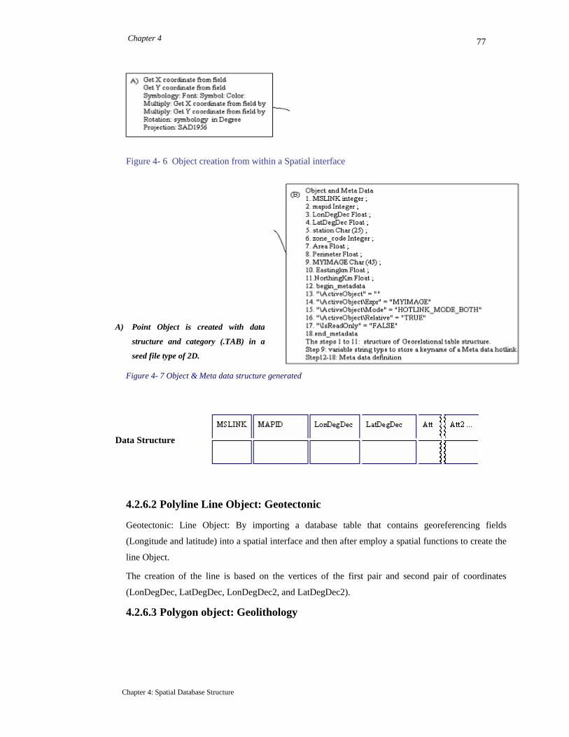
Chapter 4 77

Figure 4- 6 Object creation from within a Spatial interface

A) Point Object is created with data

structure and category (.TAB) in a

seed file type of 2D.

Figure 4- 7 Object & Meta data structure generated

Data Structure

4.2.6.2 Polyline Line Object: Geotectonic

Geotectonic: Line Object: By importing a database table that contains georeferencing fields

(Longitude and latitude) into a spatial interface and then after employ a spatial functions to create the

line Object.

The creation of the line is based on the vertices of the first pair and second pair of coordinates

(LonDegDec, LatDegDec, LonDegDec2, and LatDegDec2).

4.2.6.3 Polygon object: Geolithology


Chapter 4 78

a) By importing a database table that contains sorted georeferencing fields (Longitude and latitude)

into a spatial interface and then after employ a spatial functions that create the polyline and later

convert the polyline to polygon Objects.

b) Utilizing feature Creation Tools >> for instance Create polygon Tool (MBE)

4.2.6.4 Update Spatial Data Object (Point to Centroid)

Update Location Point

Set Obj = Create Circle (LonDegDec, LonDegDec, Unit)

The Point Object is converted into a circle with a specific filed radius in U (unit).

C) Update Circle Object

Set Obj= Create Point (Centroid (Obj)), (Centroid (Obj))

Output will be Point Object.

If seed file type is 3D type, then an elevation attribute is incorporated.

Test Results


Chapter 4 79

Figure 4- 8 Test Results Point Objects

4.2.6.5 Update Spatial Data Object (Line)

Set Obj = Create line (LonDegDec, LatDegDec, LonDegDec2, LatDegDec2)


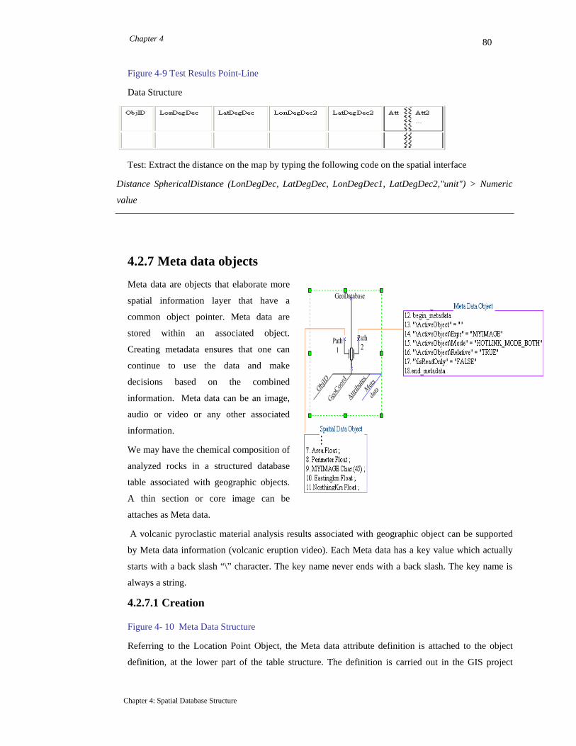
Chapter 4 80

Figure 4-9 Test Results Point-Line

Data Structure

Test: Extract the distance on the map by typing the following code on the spatial interface

Distance SphericalDistance (LonDegDec, LatDegDec, LonDegDec1, LatDegDec2,"unit") > Numeric

value

4.2.7 Meta data objects

Meta data are objects that elaborate more

spatial information layer that have a

common object pointer. Meta data are

stored within an associated object.

Creating metadata ensures that one can

continue to use the data and make

decisions based on the combined

information. Meta data can be an image,

audio or video or any other associated

information.

We may have the chemical composition of

analyzed rocks in a structured database

table associated with geographic objects.

A thin section or core image can be

attaches as Meta data.

A volcanic pyroclastic material analysis results associated with geographic object can be supported

by Meta data information (volcanic eruption video). Each Meta data has a key value which actually

starts with a back slash “\” character. The key name never ends with a back slash. The key name is

always a string.

4.2.7.1 Creation

Figure 4- 10 Meta Data Structure

Referring to the Location Point Object, the Meta data attribute definition is attached to the object

definition, at the lower part of the table structure. The definition is carried out in the GIS project


Chapter 4 81

table’s row as a text to store the path of the object that would be used to give further information

about the spatial layer. The populated path of the Meta data points to the location of the hot link while

it is bound to the same object identifier. Based on the generated structure the hotlink is stored as of

Label, Object, or both [30] as indicated bellow.

Querying the table that stores the information can retrieve Meta data. The process includes setting the

attribute to the keyname and triggering the event that opens the Meta data item, see chapter 6.

Data structure

4.2.8 Spatial Database Operations

4.2.8.1 Object Decomposition and Mending

At a time where two or more polygons coexists representing different information, extra line creation

adjacent to each polygon, as a means of demarcating polygons from each other is redundant since it

creates buffer zone and it consumes extra space.

Figure 4- 11

Decomposition of

polygon boundaries

Hence, these

superfluous lines

boundary must be

mended to represent

a single boundary

in between the two

and such mending

of the topologic

features is

accomplished

before the

association of database records with the respective features. Referring to figure 4-14, the geometry is

composed of three polygons (V, Z, and Y) with undefined polygonal boundary. They are neighbored

by the adjacent line S4 as a boundary between Polygons V and Z and S6 between Z and Y

respectively.


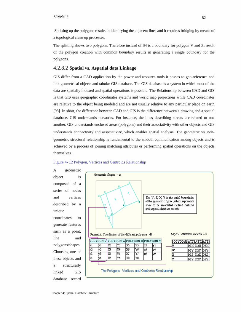
Chapter 4 82

Splitting up the polygons results in identifying the adjacent lines and it requires bridging by means of

a topological clean up processes.

The splitting shows two polygons. Therefore instead of S4 is a boundary for polygon V and Z, result

of the polygon creation with common boundary results in generating a single boundary for the

polygons.

4.2.8.2 Spatial vs. Aspatial data Linkage GIS differ from a CAD application by the power and resource tools it posses to geo-reference and

link geometrical objects and tabular GIS database. The GIS database is a system in which most of the

data are spatially indexed and spatial operations is possible. The Relationship between CAD and GIS

is that GIS uses geographic coordinates systems and world map projections while CAD coordinates

are relative to the object being modeled and are not usually relative to any particular place on earth

[93]. In short, the difference between CAD and GIS is the difference between a drawing and a spatial

database. GIS understands networks. For instance, the lines describing streets are related to one

another. GIS understands enclosed areas (polygons) and their associativity with other objects and GIS

understands connectivity and associativity, which enables spatial analysis. The geometric vs. non-

geometric structural relationship is fundamental to the smooth communication among objects and is

achieved by a process of joining matching attributes or performing spatial operations on the objects

themselves.

Figure 4- 12 Polygon, Vertices and Centroids Relationship

A geometric

object is

composed of a

series of nodes

and vertices

described by a

unique

coordinates to

generate features

such as a point,

line and

polygons/shapes.

Choosing one of

these objects and

a structurally

linked GIS

database record


Chapter 4 83

is fundamental to the hatching of geo-reference able information.

Referring to figure 4-12, every polygon is composed of a number of vertices in which the intersection

of the line makes a point at X and Y coordinates.

The polygon V (see figure 4-9) contains 4 vertices represented by x1; y1 …x4, y4 and a close loop of

the vertices produces a polygon. That polygon B (V) is described by its polygon ID and is attached to

database record C (v).

If the feature is a point type feature, then each point object can also be associated to attribute records,

which can be spatially georeferenced by a point rather than by a polygon.

For instance, in the case study GIS (Guayaquil project), measurement stations represented by latitude

longitude coordinates, which are represented by points, associated to a linked Gua.mdb.

The connected lines at a given vertex pertaining to the given shape determine every polygon limit.

Meanwhile its own spatial identifier identifies each polygon.

Thus, inter-connetiontion of the aspatial file with the geometric figures as depicted in figure 4-9

resulted in the founding of spatial-aspatial linkage (see figure 4-13).

Polygon-Coordinate-Attributes Relationship

Figure 4- 13 Polygon-Coordinate-Attributes Relationship

4.2.8.3 Spatial Integration

GIS tools have the capability to dissolve a common boundary during a process of thematic buffering

[20]. For example, it is possible to merge polygons together that have them same land use attribute.

This would enable to see continuous areas where land use type could be of the same.


Chapter 4 84

Figure 4-14 Spatial Assimilation

In the same analogy, the polygons (see figure 4-14) are demonstrating the application of thematic

merging by means of gauging the variation in a rock forming composition. During thematic

analysis on polygons, which are adjacent to each other and have similar characteristic, then, the

theme attribute values can be visualized with uniform thematic symbols by dissolving the

boundary between them.

4.2.8.4 Binding Geographic Objects

Case: MicroStation Geographics: - (The

feature names reveal textual descriptions of

(see chapter 3) geographic objects, such as

shapes, lines, points or text nodes which are

associated to the textual feature. The property

of geographic objects can be displayed by

attaching the textual feature description to the

object by a means of feature building

functions. There are two types of feature

attach

Figure 4-15 Binding:- Graphic feature

description, (II)-Spatial Objects vs. DB

records

ment.


Chapter 4


85

I. Geographic Elements vs. Descriptive feature attachment: Defined in the project feature set-up

and is related to a specific category. The feature description is stored within the system-generated

feature table.

The spatial functions (attach and detach) are triggered from within the geographic interface. The

textual description attached to the geographic object used to decipher the content of object upon

clicking it, (see figure 4-15).

II- Database Record vs. Features Attachment: The structured database records are appended and

assimilated to the geographic object after the attach operation.

For instance, the database record stored in the feature (object) Location required to be attached to its

centroid with specific OBJID is extracted

Extraction: = SELECT * FROM LOCATION WHERE OBJID = 1;

The query releases the result that corresponds to the geo-referencing coordinates.

ObjID MapID LonDeg LonDeg CurrentSpeed MeasUnit1 1 -2:30:45 -79:25:43 300 cm/sec Cm/sec

Table 4- 3 Query Result

Activating object Measurement point (figure 4_15) and executing the ATTACH function will

automatically result in assimilating the record within the Geographic object. This process is similar to

the joining of an object and tabular information for spatial visualization. Furthermore, the attribute

Talias in the Ugtable_Cat is used here to keep the consistency and integrity of the GIS information

extraction by referencing the value of an attribute to its specific table.

Case ArcView GIS: In the case of ArcView, the feature Identifier can migrate as a Foreign Key and

a join of the spatial object and aspatial database records is established. Linking or joining the database

records depends on the cardinality relationship between the .dbf or .txt files and the ObjID for the

respective feature type.

A relationship of type 1: M preferred type of association = LINKING

A relationship of type 1:1 preferred type of association = JOIN

Associating in a join of (1: M) results associated database records ONLY equal to the ObjID values.

Linking enables to georefrence the database records associated to the feature but with no thematic

displays. Event table with specific geodata source is directly loaded to generate point features if it

adheres to the 1:1 mapping principle.

GIS Applications Data files Processing Tools Outputs

MGE RDB Tables, ASCII Files MGAL, macro, manual Associated Point feature

GIS

Data

Popu

lat

Poss

ibiliti

es

Geographic RDB Tables, ASCII Files Macro, MBE, manual Associated Point feature

Chapter 4 86

ArcView RDB Tables, ASCII Files Importing, link Associated Point feature

MapInfo RDB Tables, ASCII Files Importing, link Associated Point feature

Table 4- 4 Populating the GIS environments

4.2.9 Topology Cleanup processes

4.2.9.1 Topologically cleaned Maps

The aim of topology operation is to clean up maps in order to ensure the integrity of information, and

perform successful spatial analysis. The topological relationship is determined with regard to the

purpose of the GIS designed. Many unnecessary line elements may stem out during digitizing

process, as consequence of converting of maps from one format to the other (e.g. .DGN to DXF).

Eventually this may influence the topology relationships [25] because bounding elements between

areas required to adhere to the process of GIS map construction, which includes performing

topological clean up to remove the undesired line fragments and connectivity.

The following examples are related to the topologic clean up operations [11].

4.2.9.2 Snapping and Cleaning line fragments

Generally, GIS is equipped with topological clean up

tools designed to find, modify and mend the

unnecessary elements. They work on a line, Line

strings, curves, and shapes. The tools in the case

study, based on [11] were utilized to detect and

update conditions outlined 1-6.

1. Duplicate line works 2. Similar line works, 3. Line fragments 4. Linear line segmentation 5. Finding gaps 6. Finding dangles

4.2.9.3 Duplicate line

A duplicate line (DL) is a linear element that shares the same coordinates as another linear element. A

DL may differ by assigning a Level, View and element symbology, so that they can be turned on and

off during the phase of attribute database record linkage and visualization. FIND DUPLICATE

LINKWORK TOOL locates the DL and moves to a new level for appropriate operations indicated

below.

Key-in: FENCE MOVE DUPLICATES [Level=n]

Key-in: FENCE DELETE DUPLICATES

Key-in: FENCE MERGE DUPLICATES

Fence: a fence on the target element

Move, delete and merge: are the underlying procedure calls.


Chapter 4 87

N: number of a level (related 63 view levels).

4.2.9.4 Similar Line-work (SL)

A similar line work is a line that occupies a common area as the other line, almost identical or is

partially over lapping. The similar line is detected by generating a zone specified tolerance value, (see

figure 4-16).

The output of the operation is singling out of the similar line fragments.

Key-in: FENCE MOVES SIMILAR [Toler=t] [Percent=p] [Level=l]

Key-in: FENCE DELETE SIMILAR [Toler=t] [Percent=p]

Key-in: FENCE FLAG SIMILAR [Toler=t] [Percent=p] [Color=c] [Weight=w] [Level=l]

Figure 4-16

Locating map’s

Similar Line-work

4.2.9.5 Line fragments (LF)

Line fragments are the riffraff elements that posses specific x, y coordinates that occur within a range

of specific tolerance during unstable digitizing process.

Key-in: FENCE MOVE FRAGMENTS [Toler=t] [Level=l]

Key-in: FENCE DELETE FRAGMENTS [Toler=t]

Only the line fragment that meets the criteria of the specified tolerance value moved into specified

level (L) (see figure 4-17, to find and clear the line fragments.


Chapter 4 88

Figure 4-17 Avoiding LF : 1-raw map, 2-detected line fragments, 3-toplogically cleaned.

4.2.9.6 Linear Segmentation (LS)

A topological tool is used to create a network of distinct line segments between each pair of

intersection or junction points. Operations related to this process include: -

Self: breaks lines that are self-intersect element at the cross over points.

Split: breaks overlapping linear elements at their intersection point to create linear elements.

Elements: segments elements at point of intersection or near point of intersection if the gap meets

the required tolerance.

Figure 4- 18 Segmenting Geographic Elements


Chapter 4 89

As a result of segmentation the input of two-line segment resulted to 4-segmented lines, (see figure 4-

18), which are eventually to be tagged and associated with 4 unique object identifiers.

4.2.9.7 Gap among spatial elements (G)

Proximally located linear elements should share a common end point to close the gap among them.

Thematic resymbolisation of areas or polygons is based on shapes.

Topologically, closed curves must be converted to shapes so that thematic visualization can be

possible. The gap closing process requires the definition of tolerance to snap the two-end endpoint

together. See illustration: Gap Tolerance setting-

Step 1 tolerance = user option

Test for 1, Gap value (A= 4) 2, Gap value (B= 7): - for a tolerance value of 4, gap A will be mended,

whereas B will not. So, as a function of tolerance value, a gap size is detected and shape mended. See

figure 4_19.

F (TolVal) > = (gVal) = gap repaired and F (tolVal) < = (gVal) gap not affected.

Figure 4- 19 Gap and Tolerance Size

Depending on the gaps among geographic elements, changing the value of the tolerance changes the flags

of gaps detected, then gaps detected corresponding to the specified tolerance (See Figure 4-20 (A); in step

1, two gaps and two dangles lines are corrected and the shape is created. By increasing the tolerance

value on step 2 (see figure.4-20B) to 1.000 the remaining gaps with higher values are flagged, eventually

transferred to a correction chamber.


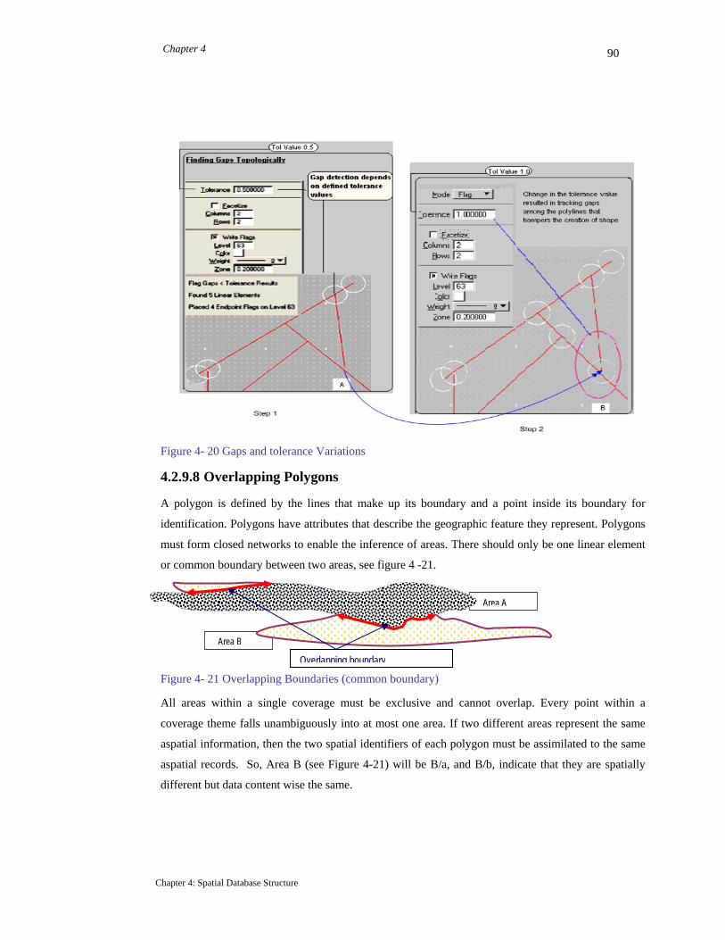
Chapter 4 90

Figure 4- 20 Gaps and tolerance Variations

4.2.9.8 Overlapping Polygons

A polygon is defined by the lines that make up its boundary and a point inside its boundary for

identification. Polygons have attributes that describe the geographic feature they represent. Polygons

must form closed networks to enable the inference of areas. There should only be one linear element

or common boundary between two areas, see figure 4 -21.

Area A

Area B

Overlapping boundary

Figure 4- 21 Overlapping Boundaries (common boundary)

All areas within a single coverage must be exclusive and cannot overlap. Every point within a

coverage theme falls unambiguously into at most one area. If two different areas represent the same

aspatial information, then the two spatial identifiers of each polygon must be assimilated to the same

aspatial records. So, Area B (see Figure 4-21) will be B/a, and B/b, indicate that they are spatially

different but data content wise the same.


Chapter 4 91

4.3 Results and Conclusions Structuring turns data into information, improves the way in which a large data are amassed

persistently in the Geodatabase, and enhances retrieving efficiency and maintenance respectively.

The Object Relational structure data model is flexible for the spatial data management because of

its capability in storing objects, implementing SQL, SQL3, and incorporating user defined functions

(UDF) and spatial operators to extract, display and perform spatial analysis.

The associativity of geometric objects and structured attribute tables requires a meticulous

preparation. One mandatory process is checking for topological incompatibility (unnecessary gaps,

overlapped polygons, presence of under or over shoots) of building block features, which has been

implemented using topology clean up tools.

Topology operation is indispensable to perform and achieve an appropriate object relational

analysis and visualization of the information spatially.

Overlapping of geographic objects could stem out of poorly represented boundary matches.

Overlapped objects cause undesired ambiguity and misleading results during spatial interpretations.

Creating clear topology relationships between objects before the action of spatial and aspatial data

integrations have settled this problem.


Chapter 5

Chapter 5: Constructing the GIS Maps

92


5.1 Introduction Obviously, maps are the primary components of GIS. Their production requires knowledge of geo-mapping

based on the principles of cartography, field surveying and spatial database managements. Typically, they

could be of raster or vector electronic file types. The type and dimension of maps varies depending on the

intended purpose. This chapter undertakes issues pertaining to appropriate GIS map generation within the

scope and relevance to this research work.

Currently, different mapping software packages are being designed to draw and produce digital maps,

example a CAD. However, such application is limited to graphical display, outputs non-relevant to spatial

analytical capabilities when matched up to GIS, which is created to integrate multidisciplinary data and

perform spatial analysis.

Creating full-fledged GIS maps involves storing data in a computer, in a digital form. The process requires a

sequence of processes, such as, scanning, digitizing, geo-registering and amalgamating with structured

databases.

Figure 5-1, is an illustration of GIS map of the northern part of Guayaquil Estuary (GIS case study), which

depicts vectorised tributary flanks overlaying a satellite image and labeled measurement sites ( 17). The

different color indicates different information on the ground.

GIS maps which are composed of features are valuable for

performing thematical display of integrated information

layers [10]. Also a raster base map (composed of pixels) can

be vectorised, and the output be applied to perform discrete

spatial analysis of the associated database records for that

specific area. Eventually, this fact enables us to evaluate

visually discrete status of the target area. With this regard, it

is natural to stress that the accuracy of GIS maps is vital not

only for the intention of depicting geo-referenceable

processed data but also for making important topologically

related spatial decisions akin to public and private spatial

assets.

Figure 5-1 Raster-Vector Overlap: Northern Guayaquil GIS Map

Examples: delineate zones susceptible to hazardous

environment, demarcating fertile soil types and potential of

economic resources, identify coastal zones with high

demographic pressure, navigate and monitor remote

research areas, urban and rural traffic managements …etc.

Chapter 5


93

The means of generating discrete geo-reference able features in the form of vector elements by

digitizing satellite images, scanned photos, numerical value derivative mapping, (2D and 3D) necessitates

projection of research maps.

5.2 GIS Maps (Vector and Raster)

overshoots

Vector dataRepresentaion

Raster dataRepresentaion

pixel

Vector map: It is composed of points, lines, and polygons, is an abstraction of the real world where

positional data is represented in the form of x and y coordinates [21]. Point is represented by a Cartesian

coordinates of x and y. Line is composed of series of ordered points. Polygon is represented as ordered list of

points; with beginning and ending points are made to coincide

in the same node and closed to create a defined polygon.

Vector maps require complex data structure but occupy less

storage space. However, maintaining topological relationship

is easier especially when compared with raster based GIS, see

figure 5-2.

Figure 5 - 2 Maps representation

Raster Map: Raster based maps (systems) are composed of a matrix of pixels. Pixel refers to the smallest

unit of information available in an image [25]. A unique reference coordinate represents each pixel and

posses a discrete attribute assigned to it. Resolution depends on either the grid size or pixel and may vary

from sub meters to kilometers [11], [21]. The resolution of the coastal satellite image in this research work is

of 30 meters.

5.2.1 Scanning Pre-Existing Maps

Scanning is a process utilized to convert objects (e.g. paper

maps) into image files. It is also equated to a means of

sampling images with different color intensity. The paper map

[see figure 5-3] is extracted from geo-scientific report related

to stratigraphic, Sedimentology and Tectonics of Ecuador

[16]. It has been scanned in an optical scanner of flat bed type

and later digitized on a computer screen with proper

registration [21], utilizing the area’s projection Datum.

Working on raster based maps is advantageous in the fields of

Soil, forestry, rock types, marine and sub marine volcanology

GIS to mention few; but there are some short comings which

crops out as in the following (case 1-case 4).

Figure5 - 3 Scanned Paper map

Chapter 5


94

Case 1 - The whole scanned image is converted to a single layer; hence, the apparently

visible different colors within the image are dictated to be a single layer.

Case 2 - Case 1 causes difficulties to distinct a river boundary and the measurement point features,

which can be associated with database record (in a feature based GIS).

Case 3 - In an image, a boundary can be visualized as a distinct set of specific pixel with specific

color but it can’t be relocated as a feature with a specific symbology.

Case 4 - Raster files are large and can consume huge space in the system.

5.2.2 Vectorising

Converting images (see figure 5-3) into a distinct feature

based map is a process of digitizing (see figure 5-4). This

process has been executed on the scanned coastal map. Any

scanned image with proper format can be viewed in a

computer screen using an image viewer, manipulated (zoom,

cut, paste…) and digitized appropriately. During digitizing the

coordinates of every digitized element on the image are placed

in a separate level with distinct symbology that identifies

uniquely. This process can also be accomplished utilizing

macros. Figure 5-4 is a display of the digitized and

topologically cleaned and geo-referenced coastal map.

Figure 5-4 Vectorised and Topological clean up

5.2.2.1 Automated Scanning

Macro based digitized map is based on geo-coordinates corresponding to the underlying registered image

file, (see figure 5-5). The vertices are joined to form lines (using mbe, see figure 5-5) that can be used as

features during the GIS construction process.

Figure5 -5 digitizing process

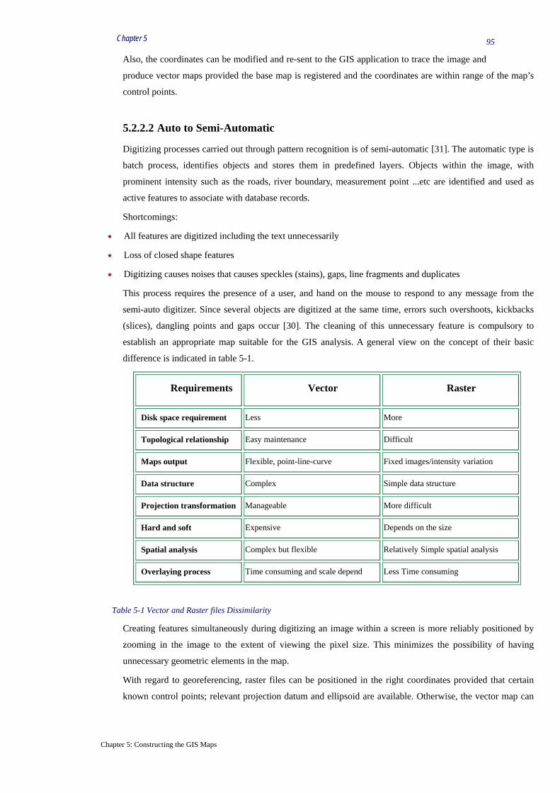
Chapter 5


95

Also, the coordinates can be modified and re-sent to the GIS application to trace the image and

produce vector maps provided the base map is registered and the coordinates are within range of the map’s

control points.

5.2.2.2 Auto to Semi-Automatic

Digitizing processes carried out through pattern recognition is of semi-automatic [31]. The automatic type is

batch process, identifies objects and stores them in predefined layers. Objects within the image, with

prominent intensity such as the roads, river boundary, measurement point ...etc are identified and used as

active features to associate with database records.

Shortcomings:

All features are digitized including the text unnecessarily

Loss of closed shape features

Digitizing causes noises that causes speckles (stains), gaps, line fragments and duplicates

This process requires the presence of a user, and hand on the mouse to respond to any message from the

semi-auto digitizer. Since several objects are digitized at the same time, errors such overshoots, kickbacks

(slices), dangling points and gaps occur [30]. The cleaning of this unnecessary feature is compulsory to

establish an appropriate map suitable for the GIS analysis. A general view on the concept of their basic

difference is indicated in table 5-1.

Requirements Vector Raster

Disk space requirement Less More

Topological relationship Easy maintenance Difficult

Maps output Flexible, point-line-curve Fixed images/intensity variation

Data structure Complex Simple data structure

Projection transformation Manageable More difficult

Hard and soft Expensive Depends on the size

Spatial analysis Complex but flexible Relatively Simple spatial analysis

Overlaying process Time consuming and scale depend Less Time consuming

Table 5-1 Vector and Raster files Dissimilarity

Creating features simultaneously during digitizing an image within a screen is more reliably positioned by

zooming in the image to the extent of viewing the pixel size. This minimizes the possibility of having

unnecessary geometric elements in the map.

With regard to georeferencing, raster files can be positioned in the right coordinates provided that certain

known control points; relevant projection datum and ellipsoid are available. Otherwise, the vector map can

Chapter 5


96

be positioned - (A) by creating projected grid based on a control points and hook the tips of the

grid to the target map (map to be projected). (B), by projecting individual features during the definition of

the objects, which a major importance of the object relational data management.

In terms of the spatial geodatabase construction and related spatial analysis, the topologically cleaned

features can be associated to individual geodatabase records based on the assigned ObjectID and geometry

type. Furthermore, the features can be thematically represented by different symbols to represent the content

of the associated, statistically classified geodatabase records.

Creating features from initially shrunken image will create discrepancy in the accuracy of the geo-referenced

locations and thus creates ambiguity in the reality of the GIS analysis and interpretation process.

5.3 Case Study: Guayaquil Estuary

5.3.1 GIS Map’s Features

In this case, study; the feature maps (see

figure 5-6) are those that represent the real

world objects associated to structured

database records. They are described as

types of line, polyline, polygon and text.

Their symbology includes, the level

situated, color, style, weight and the

tolerance and priority of display. The

vector map representation was chosen, for

it is convenient to locate geographic

objects that represent distinct area of

interest (area or perimeter, point of

measurement, boundary (contact zone),

extension and direction of a tectonic

shears) with specific element type

description and symbology (see figure 5-

6).

Figure5-6 Composite lithologic and Tectonic

and Location Points

5.3.1.1 Coastal Geo-Lithology

According to the literature [16], the

coastal geo set up of Guayaquil area is comprised of: -

Oceanic crust composition (basaltic), and theoletic type; harzuburgite outcrops with pyrite and

rarely copper dissemination; andesitic and dasitic basalt, dissected by dykes intrusive of granite.

Unconsolidated sediments of sand, silts and clay, silt stone, lenticular layers of calizas algae

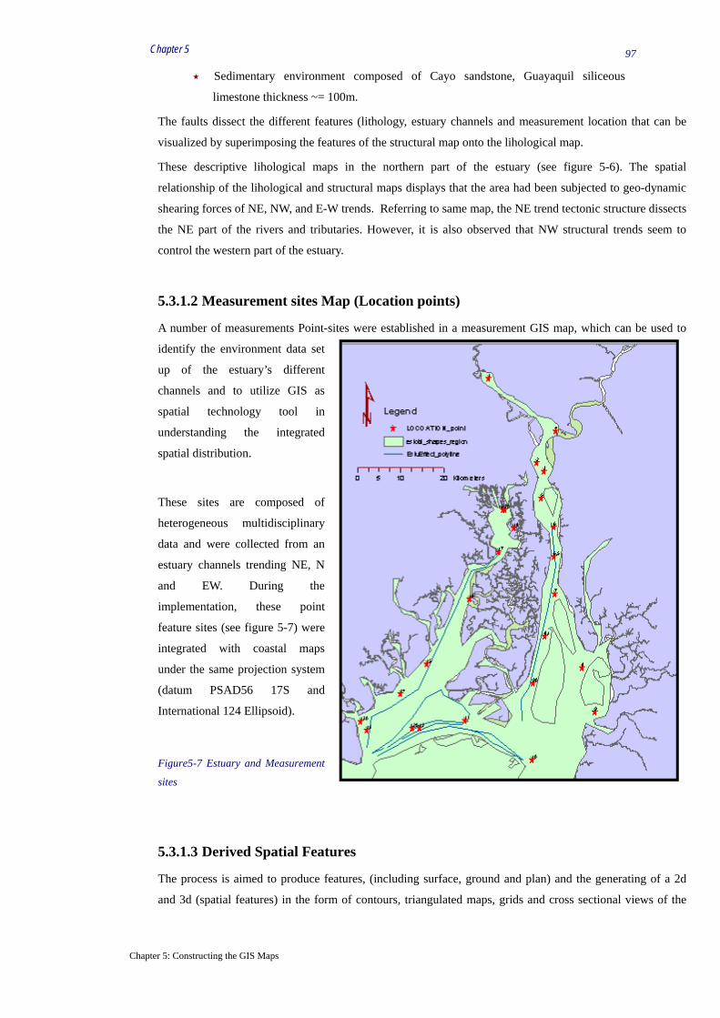
Chapter 5


97

Sedimentary environment composed of Cayo sandstone, Guayaquil siliceous

limestone thickness ~= 100m.

The faults dissect the different features (lithology, estuary channels and measurement location that can be

visualized by superimposing the features of the structural map onto the lihological map.

These descriptive lihological maps in the northern part of the estuary (see figure 5-6). The spatial

relationship of the lihological and structural maps displays that the area had been subjected to geo-dynamic

shearing forces of NE, NW, and E-W trends. Referring to same map, the NE trend tectonic structure dissects

the NE part of the rivers and tributaries. However, it is also observed that NW structural trends seem to

control the western part of the estuary.

5.3.1.2 Measurement sites Map (Location points)

A number of measurements Point-sites were established in a measurement GIS map, which can be used to

identify the environment data set

up of the estuary’s different

channels and to utilize GIS as

spatial technology tool in

understanding the integrated

spatial distribution.

These sites are composed of

heterogeneous multidisciplinary

data and were collected from an

estuary channels trending NE, N

and EW. During the

implementation, these point

feature sites (see figure 5-7) were

integrated with coastal maps

under the same projection system

(datum PSAD56 17S and

International 124 Ellipsoid).

Figure5-7 Estuary and Measurement

sites

5.3.1.3 Derived Spatial Features

The process is aimed to produce features, (including surface, ground and plan) and the generating of a 2d

and 3d (spatial features) in the form of contours, triangulated maps, grids and cross sectional views of the

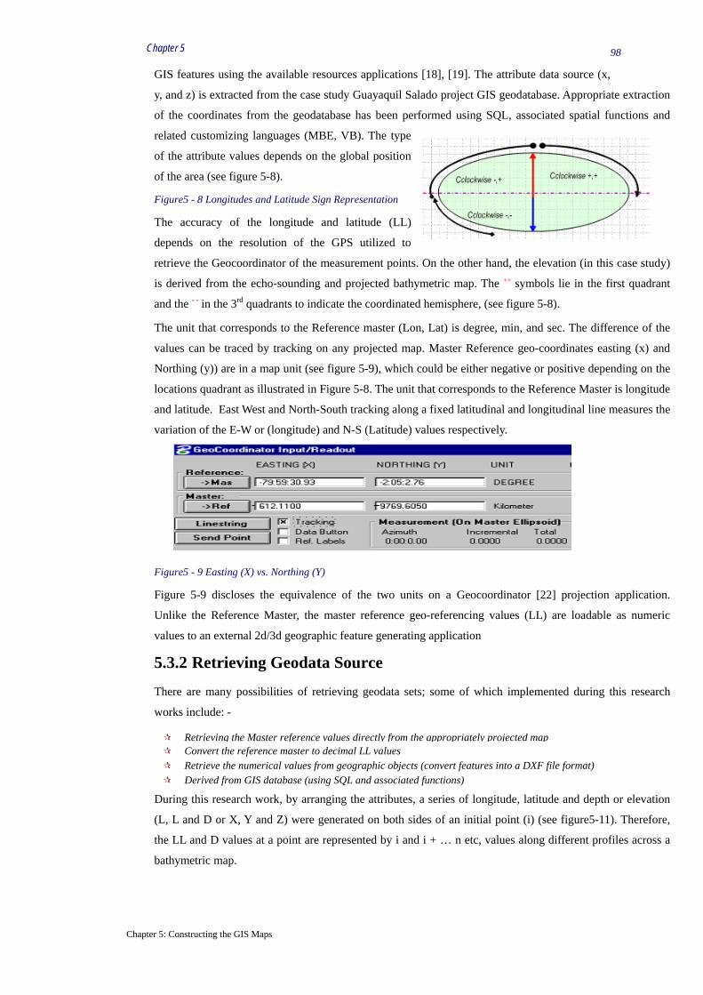
Chapter 5


98

GIS features using the available resources applications [18], [19]. The attribute data source (x,

y, and z) is extracted from the case study Guayaquil Salado project GIS geodatabase. Appropriate extraction

of the coordinates from the geodatabase has been performed using SQL, associated spatial functions and

related customizing languages (MBE, VB). The type

of the attribute values depends on the global position

of the area (see figure 5-8).

Figure5 - 8 Longitudes and Latitude Sign Representation

The accuracy of the longitude and latitude (LL)

depends on the resolution of the GPS utilized to

retrieve the Geocoordinator of the measurement points. On the other hand, the elevation (in this case study)

is derived from the echo-sounding and projected bathymetric map. The ++ symbols lie in the first quadrant

and the - - in the 3rd quadrants to indicate the coordinated hemisphere, (see figure 5-8).

The unit that corresponds to the Reference master (Lon, Lat) is degree, min, and sec. The difference of the

values can be traced by tracking on any projected map. Master Reference geo-coordinates easting (x) and

Northing (y)) are in a map unit (see figure 5-9), which could be either negative or positive depending on the

locations quadrant as illustrated in Figure 5-8. The unit that corresponds to the Reference Master is longitude

and latitude. East West and North-South tracking along a fixed latitudinal and longitudinal line measures the

variation of the E-W or (longitude) and N-S (Latitude) values respectively.

Figure5 - 9 Easting (X) vs. Northing (Y)

Figure 5-9 discloses the equivalence of the two units on a Geocoordinator [22] projection application.

Unlike the Reference Master, the master reference geo-referencing values (LL) are loadable as numeric

values to an external 2d/3d geographic feature generating application

5.3.2 Retrieving Geodata Source

There are many possibilities of retrieving geodata sets; some of which implemented during this research

works include: -

Retrieving the Master reference values directly from the appropriately projected map Convert the reference master to decimal LL values Retrieve the numerical values from geographic objects (convert features into a DXF file format) Derived from GIS database (using SQL and associated functions)

During this research work, by arranging the attributes, a series of longitude, latitude and depth or elevation

(L, L and D or X, Y and Z) were generated on both sides of an initial point (i) (see figure5-11). Therefore,

the LL and D values at a point are represented by i and i + … n etc, values along different profiles across a

bathymetric map.

Chapter 5


99

Linearly: = ( ) ( ) ( ) )2/,2/,2/( ZnZYnYXnXi ±±±=

Figure5 - 10 Generating the 3D parameters

The attribute data that control the 3d surface generation has been created, taking into account the original

values of OE, ON, OD (see figure 5-10, and 5-11) at a given point within a projected working map. For a

fixed azimuthal direction (ON) there is a change on OE + - n and change of elevation on (OD).

Figure5 -11 (A) Initial point of reference (B) extending (C) increment

5.3.2.1 Converting the Typed data

String type input (reference master values) of longitude and latitudes cannot be included into the calculations

as they are. They ought to be converted into numeric values using extended SQL programs so that they can

be included into the program calculation, see below the

procedure applied. The conversion process includes

following steps: -

(A) Step1 - Step2 selects the attributes from the table,

Step3 - Step8 extracts the longitude, latitude numeric

values and coins the name LonDeg, and LatDeg, LonMin and LatMin, and LonSec and LatSec for degree,

minute and seconds respectively. The converted values

are populated in the geodatabase with variables OE,

ON, OD and further can be extracted in a sorted order

to generate the geometric elements.

B) The program generates coordinates values converted

and arranged in a series of ordered X (OE) and Y (ON)

and respective Z (OD) coordinates with respect to original point of reference (Easting (X), Northing (Y) and

elevation (Z), (see figure 5-12)

X, Y, Zn

I X Y, Zn + 1

Chapter 5


100

Figure5 - 12 Illustrating the process

The ON, OE and OZ are the initial or departure point references for recording the different elevation with

respect to the change of the longitude and latitude coordinates. They ON+1, OE, OZ+1 indicate a move

along the Northing, with no change of easting but change on elevation. The ON, OE+1, OZ+1 shows the

shifting of the position eastwards with constant Northing as the initial point but with possible change on the

elevation. In a similar manner, the leftward and rightward extension with respect to the possible changes of

the elevation is indicated below, (see table 5-2).

5.3.2.2 Graphic data generation

Based on the procedure (section 5.3.2.1) the measured values of the co-ordinates and the corresponding

elevation values are retrieved from the structured database. The values generated are loaded into a Macro to

create a regular grid system for the geographic features that represent the GIS measurement points. Table 5-2

(a+b) shows the values corresponding to the variables defined in the database.

Table 5-2 (a) Geodata source (b) Extended 3D Measured Data source

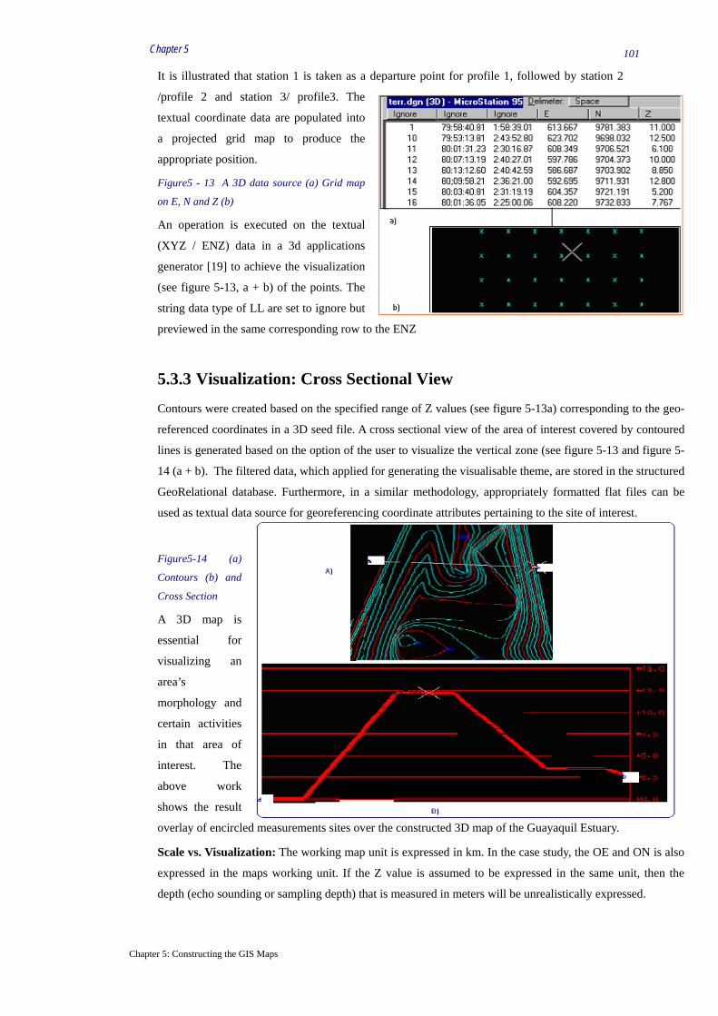
Chapter 5


101

It is illustrated that station 1 is taken as a departure point for profile 1, followed by station 2

/profile 2 and station 3/ profile3. The

textual coordinate data are populated into

a projected grid map to produce the

appropriate position.

Figure5 - 13 A 3D data source (a) Grid map

on E, N and Z (b)

An operation is executed on the textual

(XYZ / ENZ) data in a 3d applications

generator [19] to achieve the visualization

(see figure 5-13, a + b) of the points. The

string data type of LL are set to ignore but

previewed in the same corresponding row to the ENZ

5.3.3 Visualization: Cross Sectional View

Contours were created based on the specified range of Z values (see figure 5-13a) corresponding to the geo-

referenced coordinates in a 3D seed file. A cross sectional view of the area of interest covered by contoured

lines is generated based on the option of the user to visualize the vertical zone (see figure 5-13 and figure 5-

14 (a + b). The filtered data, which applied for generating the visualisable theme, are stored in the structured

GeoRelational database. Furthermore, in a similar methodology, appropriately formatted flat files can be

used as textual data source for georeferencing coordinate attributes pertaining to the site of interest.

Figure5-14 (a)

Contours (b) and

Cross Section

A 3D map is

essential for

visualizing an

area’s

morphology and

certain activities

in that area of

interest. The

above work

shows the result

overlay of encircled measurements sites over the constructed 3D map of the Guayaquil Estuary.

Scale vs. Visualization: The working map unit is expressed in km. In the case study, the OE and ON is also

expressed in the maps working unit. If the Z value is assumed to be expressed in the same unit, then the

depth (echo sounding or sampling depth) that is measured in meters will be unrealistically expressed.

Chapter 5


102

Thus, the minus (-11 meters) value, which has an actual information value in meters, is

considered as km.

Thus, the minus (-11 meters) value, which has an actual information value in meters, is

considered as km.

Figure5 - 15 Cross Sectional View

Z= (Actual depth) (m) = z *10-3

To avoid this, the visualization is executed at a scale (de-exaggerating coefficient) of 1:1/1000 i.e., the Z

value is conceptually understood that it has been de-extended by

the given coefficient to rectify with the actual depth and

perspective view. In this case the Z= 15.9222 m (rounded to 15.9 m) in meters which is displayed according

to the sub working scale (m) of the projected map.

5.3.3.1 3D Perspective View of Measurement object

Superimposing of associated measurement features and attributes values on a projected map are

advantageous because there is always synchronized matching of the measured spatial database record and

their respective position of that particularly information inside the 3D map. In such cases, the spatial

analysis will take into account the vertical dimension, which indicates the elevation environment, (see figure

5-15).

Via closer visualization of the maps (see figure 5-16 a and b), one can see the layers of the real world

features as: -

(1) a 3D map is at the base displaying the estuary geomorphology,

(2) Geo-referenced measurement points are placed at the right selected position, where all the possible

multidisciplinary data were collected and an aerial extension of associated feature surrounds each

centroid.

The bathymetric contour map layer blankets the area of study, showing variable contour width to reflect the

submarine geomorphology. Even though the process of constructing and implementing is laborious and time

consuming, but the output is very important for combined visualizations and spatial analysis, hence it is

worth doing it.

Chapter 5


103

Figure5 - 16 (a) Submarine Morphology, (b) 3D, Bathymetric and measurement stations

5.3.3.2 Automated feature generation

Macros select tools and view controls, send key-ins, manipulate dialog boxes, and modify elements. The

obvious advantage of writing a macro to perform a task that could otherwise be done manually is automating

mechanical and repetitive tasks. The macro (refer appendix C) - (A) Loads the spatial data source with

properties and symbology and (B) Generate measurement features. The steps followed are: -

Step 1: Design the macro (MBE) that loads the x, y and z values and creates and creates a synchronized

position of geographic point features, Places the feature on the specified level;

Step2: Create the feature point and second feature zone of influence as an aerial extension with a radius

defined, Changes the symbology, and ends the execution using the MbeSendReset.

Step 3: Adding Features Design that views the level of the surface water in the estuary channels, then setting Z

value (echo-depth) to 0 as follows.

Sub main MbeSendKeyin "place line" MbeSendKeyin” xy=613.928, 9781.452, 0.00" ' 1 MbeSendReset End sub

Chapter 5


104

Output:

Geographic map with the specified properties and symbology Measurement along (23 stations) Estuary channels viewed with respective to depth (m). Elevation scales de-exaggeration is described textually or geometrically (z *10-3). Possible views of the map (top view, isometric, left and right views).

Figure5 –17 Geographic Features: a) top view b) left view (Z) meters View

5.4 Georeferencing We know that the earth is not flat, yet, when we construct GIS maps, it becomes our effort to make them flat

using projection system procedures. This process of altering a spheroid or curved earth’s shapes to flat

surface triggers a problem of distortion on the original setup up of maps. The earth is not sphere (not

symmetric about its center), but it is of a spheroid-shape [70], which can be described by rotating an ellipse

(see Figure 5-18), which is characterized by its major and minor axes about its axis. The spherical

coordinates are the latitude and longitude ranging –90 to + 90 and –180 to + 180 respectively.

Figure5 - 18 (a), Semi-major axis (b) Semi-minor axis

Likewise, different measurements show different

semi-major and semi-minor axes and this in turn

creates different datums.

Thus, even if two shape files of the same scale unit (longitude and latitude) and area are treated on different

datums they will not match perfectly. The following ellipsoid constants indicate the variation of the

parameters [30]. Table 5-3 shows the international-1924 and WGS84 ellipsoids (of the local area of study)

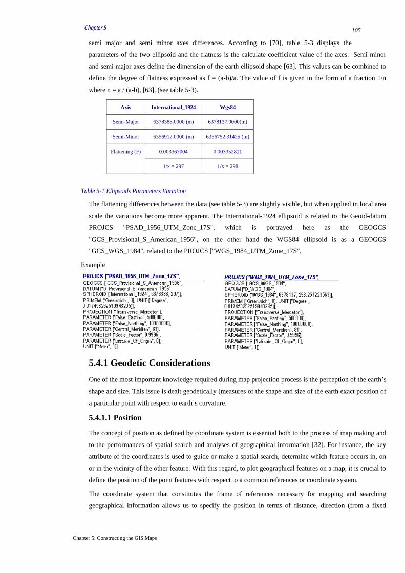
Chapter 5


105

semi major and semi minor axes differences. According to [70], table 5-3 displays the

parameters of the two ellipsoid and the flatness is the calculate coefficient value of the axes. Semi minor

and semi major axes define the dimension of the earth ellipsoid shape [63]. This values can be combined to

define the degree of flatness expressed as f = (a-b)/a. The value of f is given in the form of a fraction 1/n

where n = a / (a-b), [63], (see table 5-3).

Axis International_1924 Wgs84

Semi-Major 6378388.0000 (m) 6378137.0000(m)

Semi-Minor 6356912.0000 (m) 6356752.31425 (m)

0.003367004 0.003352811 Flattening (F)

1/x = 297 1/x = 298

Table 5-1 Ellipsoids Parameters Variation

The flattening differences between the data (see table 5-3) are slightly visible, but when applied in local area

scale the variations become more apparent. The International-1924 ellipsoid is related to the Geoid-datum

PROJCS "PSAD_1956_UTM_Zone_17S", which is portrayed here as the GEOGCS

"GCS_Provisional_S_American_1956", on the other hand the WGS84 ellipsoid is as a GEOGCS

"GCS_WGS_1984", related to the PROJCS ["WGS_1984_UTM_Zone_17S",

Example

5.4.1 Geodetic Considerations

One of the most important knowledge required during map projection process is the perception of the earth’s

shape and size. This issue is dealt geodetically (measures of the shape and size of the earth exact position of

a particular point with respect to earth’s curvature.

5.4.1.1 Position

The concept of position as defined by coordinate system is essential both to the process of map making and

to the performances of spatial search and analyses of geographical information [32]. For instance, the key

attribute of the coordinates is used to guide or make a spatial search, determine which feature occurs in, on

or in the vicinity of the other feature. With this regard, to plot geographical features on a map, it is crucial to

define the position of the point features with respect to a common references or coordinate system.

The coordinate system that constitutes the frame of references necessary for mapping and searching

geographical information allows us to specify the position in terms of distance, direction (from a fixed

Chapter 5


106

point), lines or surfaces. The representation can be revealed either in a two-dimensional planar

(rectangular) or three-dimensional polar coordinate.

5.4.1.2 Datum

A datum is a set of parameters defining a coordinate system and control points whose geometric

relationships are known, either through measurement or calculation [21]. In the last fifteen years, satellites

have provided geodesists with new measurements to define the best earth-fitting ellipsoid, which relates

coordinates to the earth’s center mass. The most recently widely used datum is the World Geodetic System

of 1984 (WGS84) [32], where the measurements are collected using GPS (Global Positioning System).

A datum is characterized by vertical and horizontal characteristic. Horizontal datum is the set of constants

specifying the coordinate system to which horizontal coordinates are referred to, whereas a vertical datum is

a set of constants specifying the coordinate system to which elevations are referred.

Substantial irregularities in the surface created by global mean see level (MSL) [15] is observed. These

irregularities form very gentle but massive “hills” and “valleys. This finding was made possible through the

use of GPS, a technology designed by national imagery and mapping agency (NIMA) [82]. The GPS

receivers compute and store coordinates in terms of WGS84, then transform to other datums when

information is displayed.

5.4.1.3 Mean Sea Level

The shape of the earth can also be defined by the surface of the oceans, which covers two thirds of the

Earth’s surface. The level of the oceans changes as the gravitational pull of the sun and the moon produce

the phenomena known as tides ellipsoid [80]. Compositionally, the earth is not uniform throughout. Regions

of denser material exist intermingled with regions of less dense material. As a function of the earth, mass

material the gravitational force varies unpredictably from one place to another. Result is complex undulating

shape with many peaks and valleys distributed over the entire surface of the Earth. “However, geodesists

have been able to establish an ellipsoid such that the height of the highest peaks and the depths of the

deepest valleys are in the order of 100 meters from this best fitting ellipsoid” [80]. So, Geoid, a term derived

from the Greek word meaning earthlike [25], is used to refer to the rather odd shape of the imaginary earth

shape] The Geoid approximates the mean sea level (MSL) [81].

Figure5-19 The Geoid, (After

Witold Fraczek)

The MSL is described as a

tidal datum that is the

arithmetic mean of hourly water elevations observed over a specific 19-year cycle [81]. This definition

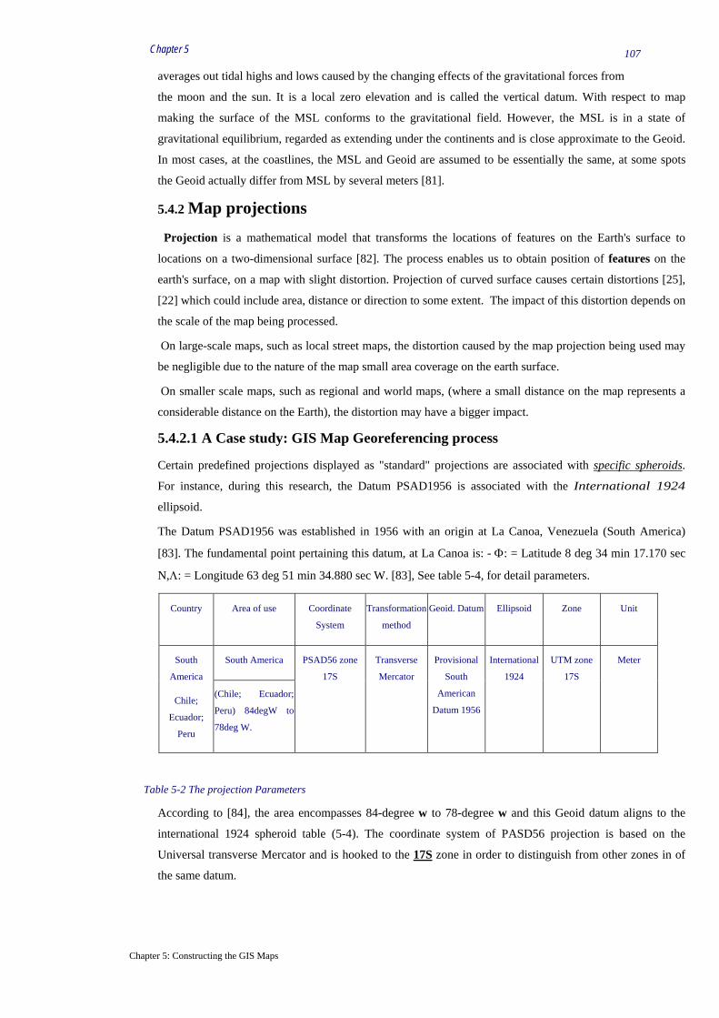
Chapter 5


107

averages out tidal highs and lows caused by the changing effects of the gravitational forces from

the moon and the sun. It is a local zero elevation and is called the vertical datum. With respect to map

making the surface of the MSL conforms to the gravitational field. However, the MSL is in a state of

gravitational equilibrium, regarded as extending under the continents and is close approximate to the Geoid.

In most cases, at the coastlines, the MSL and Geoid are assumed to be essentially the same, at some spots

the Geoid actually differ from MSL by several meters [81].

5.4.2 Map projections

Projection is a mathematical model that transforms the locations of features on the Earth's surface to

locations on a two-dimensional surface [82]. The process enables us to obtain position of features on the

earth's surface, on a map with slight distortion. Projection of curved surface causes certain distortions [25],

[22] which could include area, distance or direction to some extent. The impact of this distortion depends on

the scale of the map being processed.

On large-scale maps, such as local street maps, the distortion caused by the map projection being used may

be negligible due to the nature of the map small area coverage on the earth surface.

On smaller scale maps, such as regional and world maps, (where a small distance on the map represents a

considerable distance on the Earth), the distortion may have a bigger impact.

5.4.2.1 A Case study: GIS Map Georeferencing process

Certain predefined projections displayed as "standard" projections are associated with specific spheroids.

For instance, during this research, the Datum PSAD1956 is associated with the International 1924

ellipsoid.

The Datum PSAD1956 was established in 1956 with an origin at La Canoa, Venezuela (South America)

[83]. The fundamental point pertaining this datum, at La Canoa is: - Φ: = Latitude 8 deg 34 min 17.170 sec

N,Λ: = Longitude 63 deg 51 min 34.880 sec W. [83], See table 5-4, for detail parameters.

Country Area of use Coordinate

System

Transformation

method

Geoid. Datum Ellipsoid Zone Unit

South America South

America

Chile;

Ecuador;

Peru

(Chile; Ecuador;

Peru) 84degW to

78deg W.

PSAD56 zone

17S

Transverse

Mercator

Provisional

South

American

Datum 1956

International

1924

UTM zone

17S

Meter

Table 5-2 The projection Parameters

According to [84], the area encompasses 84-degree w to 78-degree w and this Geoid datum aligns to the

international 1924 spheroid table (5-4). The coordinate system of PASD56 projection is based on the

Universal transverse Mercator and is hooked to the 17S zone in order to distinguish from other zones in of

the same datum.

Chapter 5


108

Projection requires a grid map generation based on control points, related to a known datum and a target

map that needs georeferencing corresponding to the datum based control points, (see figure 5-20). The

intersection of x and y at a specific angle makes the map locatable. Example of such map projection grid is

the Universal Transversal Mercator (UTM) A projected coordinate system that divides the world (globe)

into 60 north and south zones, six degrees of longitude wide. Each UTM zone has its own central meridian

from which it spans 3 degrees west and 3 degrees east of that central meridian.

Figure5 -20 Map projections

The limits of each zone are 84°

N, 80° S. The origin for each

zone is the Equator and its

central meridian. To eliminate

negative coordinates, the

projection alters the coordinate

values at the origin. The value

given to the central meridian is

the false easting, and the value

assigned to the Equator is the false Northing.

For locations in the Northern Hemisphere, the origin is assigned a false easting of 500,000, and a false

Northing of 0. For locations in the Southern Hemisphere, the origin is assigned a false easting of 500,000

and a false Northing of 10,000,000.

The zone’s Northing starts at the equator as 0,000,000 and is numbered northward in meters. The easting

(longitude) coordinate is measured from an arbitrary number 500000 meters to the west of the central

meridian indicating that each central meridian is measured 500000 meters apart [27], [10].

For the southern hemisphere an offset of 10, 0000 km is applied to obtain specific coordinates. Each central

meridian is measured 50, 000 meters apart.

5.4.3 Implemented Projection Procedures

The process of the projection involved the definition of the grid and identification of the datum as given in

the operational GIS project. The steps utilized are as follows: -

5.4.3.1 Step 1: - Targeting Coordinate choice

Chapter 5


109

Figure5 - 21 Datum Specifications

The Master file coordinate system GRID was created with the Longitude and Latitudes (LL) at four corners

within an empty design file. MDL (MicroStation development language) keying is used to activate the

applications. So MDL LOAD > loads the MDL and MDL LOAD GCOORD loads the Geocoordinator

application.

5.4.3.2 Step 2: - Define Control Pnts.

Grid Generation: - Grid line parameters include - Longitude (x) and latitude (y), density of the intervals

and Min and Max values of the coordinates, level of the grid and related symbology utilized to distinguish it

from geographic features.

5.4.3.3 Step 3: Wrapping and Merging

Transformation: - Step3 involves the Merging of the projected grid with the target map user map, which has known

coordinate from the data source of the image.

Key in: - MDL LOAD MERGE (invokes merging application).

Path: - MERGE C: / ECUADOR\GUAYAS. DGN (dgn files)

Key in: - GCOORD PLACE CONTROL POINT:

1. Identify: source point = target point;

2. Map to be hooked = map in projection;

3. 4 control points selected are attached to the map

4. Warp Set-Up Fills Fills (Ctl Point);

5. Warp all (as fence) open .ctl >> transfer coordinate to target map (see figure 5-22)

6. Nailing of the 4 coordinate points of the grid to the corresponding map.

The map generated according to specified control point (4 ctl points) parameters, Datum parameters

(PSAD56) related spheroid and selected projection System (UTM). The projected grid map and the target

Chapter 5


110

map (coastal periphery map) are fused. Eventually, the projected map, (see figure 5-22), is

merged with the main estuary map as displayed in figure 5-23.

Figure5 – 22 Assimilation of a Grid and User Map

5.4.3.4 Step 4: Integrating the project maps

The area bounded by a rectangle is the newly projected map and is fitted to the main estuary map composed

of point measurement and estuary coastline geographic elements (see figure 5-23).

The performance of a perfect merging process of all the projected working features resulted to the

production of an integrated geo-referenceable map of the area of interest.

Eventually, this process facilitated the process of performing spatial analysis among the geographic

features, mainly – the measurement sites map within the Estuary and the coastal periphery maps, where the

later were derived from previous geological works, (see figure 5-23).

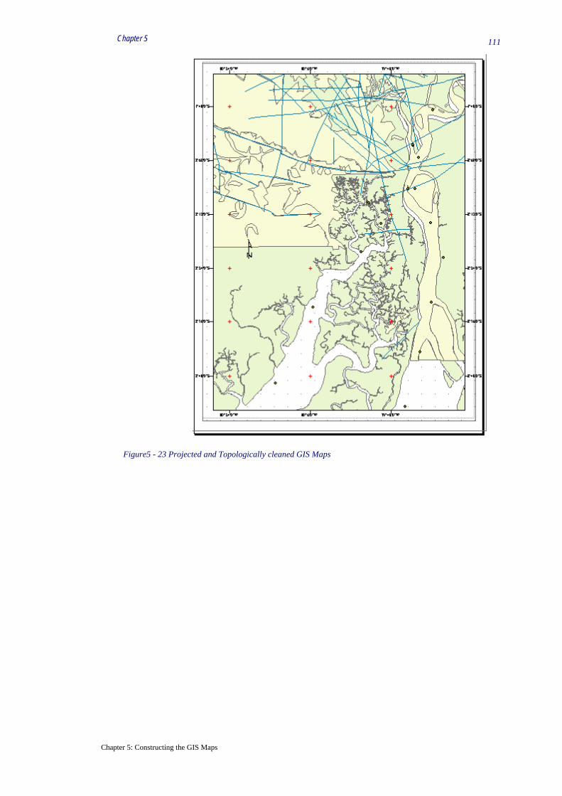
Chapter 5


111

Figure5 - 23 Projected and Topologically cleaned GIS Maps

Chapter 5


112

5.5 Results and Conclusions The Indispensability of GIS maps is not simply for depicting selected associated information but also

for making important locational and visual spatial analysis and decisions on public and private assets,

utilize in the application of sustainable environmental management, implement in the sector of mobility

of transportations and also in the identification and evaluation of economically viable potential

resources, …etc. With regard to this research work, to achieve the outlined goals, the processes of map

making (digitizing, scanning, topology and georeferencing) have been implemented.

Simultaneous digitizing and feature generating techniques have been applied to reduce the amount of

time consumed to clean maps subjected to different format conversion process.

Coastal paper maps have been scanned, vectorised, topologically cleaned and projected. Likewise, a

satellite image of the area has been registered by pin pointing known control points, conformable to the

provided PSAD56 datum.

Macro programs have been developed to generate topologically cleaned feature maps; and create 3D

GIS maps by increasing density points of observation on a 3D seed file and 3D.

The application of the developed vector and raster GIS maps were crucial to facilitate the creation of

distinct and associatable measurement features, generate thematically analyzed spatial information by

relating the developed objects and objects’ identifiers.

Chapter 6 113

Chapter 6 Spatial Analysis

Chapter 6: Spatial Analysis

6.1. Introduction

Prior to this chapter, a focus was given to the making of a GIS maps. That issue raised, that

spatial analysis (SA) performance required appropriately geo-referenced maps. Commonly,

during spatial analysis the data in the Geodatabase are examined by executing spatial operations

with the intent to create new data that fulfills some required condition(s). The process comprises

spatial operations such as polygon overlay, buffer generation, intersects, union, contains,

completely within and within distance of, and others which can be intercalated with spatial

queries. For instance, (a) the Union process creates a new theme by overlaying two polygon

themes; and (b) the completely within selects objects that fall completely within an object. Then

what is a SA?

Spatial Analysis (SA) is a technique of analyzing and visualizing associated geographic objects.

The association is mainly between geographic elements (graphic elements and tabular data). It is

vital in interpreting the results based on the model being applied [64].

SA encompasses topological operation analysis procedures for determining the spatial

coincidence of geographic features. Any collection of topology layers is assumed to share same

coordinate system to avoid unpredictable results. Once these requirements are met, spatial

analysis is implemented to obtain spatial results of selected specific problems.

Henceforth, the main theme of this chapter is to demonstrate and perform spatial analysis on the

constructed Geodatabase and illustrate the interacting objects in challenging certain selected

environmental problems.

6.2. Spatial Data Processes

GIS provides mechanisms to integrate multidisciplinary data and allows the description,

prediction and monitoring of alternative coastal management options. This is associated to its

ability to organize large volume of heterogeneous spatial, aspatial and temporal data and its

holistic visualizing power with respect to geo-referenced maps, which is indispensable for

detecting impact [44], risk forecasting, and mitigations issues.

A base map is requisite in order to perform overlay analysis under a common geo-referencing

coordinate system. To actualize the process, Geographic vector objects were created based on

longitude and latitude values by application development automating tools, such as MicroStation

Basic Extension (MBE) and Mapbasic.

Point objects were generated (see figure 6-1) to represent measurement point, such as the

BioObject, Sedobj, Heavy Metals Object… etc., whereas the Polyline and polygons represent the

coastal GeoLithology, GeoTectonic Coastline on the Guayaquil Estuary etc., and were made to

share the same coordinate system by means of a given projection datum and ellipsoid. Moreover,

the satellite image of the estuary and its surrounding has been fitted to the vector objects (see

Chapter 6 114


Explanation

For the purpose of

spatial interpretation

the Guayaquil Estuary

satellite-image map

was utilized as a

partial base map.

The overlaying vector

maps include coastline,

Estuary’s major rivers,

islands & measurement

points (red triangles)

along the estuary

channels (see figure 6-1).

figure 6-1), for the purpose of understanding the relationship of the measurements sites and raster

type maps of the coastal area.

Figure 6-1. Measurement Points

6.3. Spatial Geodatabase Communications

Geodatabase contains geographic information and provide services for managing geographic data

such as validation rules, relationships, and topological associations. Feature classes can be

organized into a feature dataset; they can also exist independently in the geodatabase. Feature

classes store geographic features represented as points, lines, or polygons, and their attributes. All

feature classes in a feature dataset share the same coordinate system [70]; hence, the information

retrieved is spatially synchronized and implemented across different GIS applications.

6.3.1 Interoperability operations Tests

Several tests of utilizing the geodatabase on different spatial engines have been performed in

order to grasp the process of possible interoperability among the spatial engines and respective

geographic objects, (see figure 6-2). At the center is the data model and the three GIS

applications are connected to exchange the spatial information with the GIS applications. The

Chapter 6 115


result depicts loss of some spatial properties during the exchange of geographic features

(especially on non Open GIS complaint). For instance, unlike the shape objects, the Data

Exchange Format, a format for storing vector data in ASCII or binary files (.dxf) and text (.txt)

objects depict a two-way communications.

GIS

DATA

MODEL

MapIn

fo

Geographic

ArcView

�

linked obj, -shapes, projection

dxf, txt fmt

Linked Obj, -Shapes,projection

dxf, txt fmt

miff,dxf -shapes,projection

dxf, txt fmt

Figure 6-2 Interoperability

This test has been executed initially, using MicroStation Geographics GIS features (dgn seed file)

and later applied in MapInfo, ArcView and ArcGIS GIS applications.

Figure 6-3 Compatibility of objects

Linked shape objects

DXF and TXT Two way exchange with preserved feature properties

There is a loss of shape and projected feature after transferring

the original seed file to other GIS application.

The associated geographic objects identified by ObjID (MSLINK) in the master coordinate bearing table are reproduced

into equal geographic features in the corresponding GIS application. E.g. Geographics >> ArcView or Geographics >>

MapInfo or MapInfo >> ArcGIS

Chapter 6 116


6.3.2 Interoperability Outputs

The tests also show that, during an exchange of the ODBC – enabled Geodatabase, linkages are

regenerated with prefixed occurrence number of the original GIS application when converted to

the other applications. For instance the ObjID (MSLINK) of the Geographic GIS would be

feature identifier with prefix for the ArcView GIS as FID =� Geo.FIDn, see table 6-1, A and B,

indicating a generic characteristics of the ObjID. Table 6-2 displays the conversion of

MicroStation Geographic GIS feature classes to a map info features. Likewise, table 6-3 discloses

the extension of the transformation process of table 6-2; MapInfo GIS features to ArcView and

ArcGIS. This illustration indicates .DGN seed file based feature is converted to a .TAB and the

.TAB to a .SHP or a .LYR respectively. During the exchange process, certain properties of the

features are preserved and lost. A summary for the process is displayed in table 6-4.

Table 6-1 Generic Characteristics of the Object Pointers

(A) Step 1

Process 1: dgn to shp Process 2:dgn to tab

MicStationGeo.Obj = ArcView.Obj MicroStaionGeog.ObjID = MapInfo.ObjID

MicStationGeo.MSLINK = ArcView.ODBC_MSLINK MicStationGeo.MSLINK = MapInfoMSLINK

DGN.link =SHP.Link DGN.link = tab. Link

(B) Step 2

Process 3: shp to tab Process 4: tab to dgn

ArcView.ObjID = MapInfo.ObjID MapInfo.ObjID = MicStationGeo.Obj

SHP.Link = tab. Link TAB.link = DGN.link

Elucidation: -

A: DGN.link=SHP.Link, DGN.Mslink=SHP.Mslink_n / Geo vs. ArcView

B: DGN.link=TAB.link, DGN.Mslink=TAB.Mslink_n / Geo vs. MapInfo

C: SHP.Link=TAB.link, SHP.FID=TAB.MIF.ID / ArcView vs. MapInfo

D: SHP.Link=TAB.link, SHP.FID=TAB.MIF.ID / ArcGIS vs. MapInfo

Transformation of MicroStation Geographics to MapInfo GIS

Table 6-2 Transformation Processes: MicroStation Geographics GIS >> MapInfo GIS

Chapter 6 117


Transformation of MicroStation Geographics >> MapInfo GIS >>ArcView and ArcGIS

Table 6-3 Extended Transformation Processes: MicroStionGeog GIS >> MapInfo >> AAGIS

The Preserved and Lost of features properties

Transformation Processes Preserved Loss

Geographic MapInfo Dxf, txt, linkage Shape, projection

Geographic ArcView Dxf, txt, linkage Shape

ArcView MapInfo DXF, txt, linkage, miff Shape, projection

MapInfo ArcView Dxf, txt, shape, projection, link Projection

MapInfo ArcGIS Shape, projection and linkage No loss

Table 6-4 Preservation and loss of Objects Properties

6.4. Spatial Information Process

Spatial-Query perception requires knowledge of the data, measurement methodology and analysis

procedures that vary on time and locatable media being measured. It is imperative to understand

that the limit of the data before the onset of the Spatial Query Formulations (SQF). Query

formulation with unrealistic data can lead to error. A GIS is a data driven application, then its

performance and usefulness is only as good as the data and the structure in which the data are

made to interact each other. For instance, the Geodatabase GIS built during this research work

accommodates variety spatial queries related to biologists, chemists, geologists …etc., because

Chapter 6 118


the data model is founded on multidiscipline perspectives. It has also been tested in different GIS

applications to evaluate the possibility of reusing the same seed file among variety spatial engines

(see table 6-3). Moreover, the efficiency of the spatial information depends on the specific GIS’s

user-friendliness of the interface. A user interface is a principal component of the GIS

application. Some GIS applications provide interface tools that permit a full-blown object

relational formulation of spatial quires and spatial interrogation to the system [37].

6.4.1 Interrogating Spatial Database Practice

Extracting spatial information is executed by posing different questions to the building block GIS

objects. To mention few, with respect to implementation of the model in the case study: -

� Find abnormal heavy metal concentration (within estuary channels)? Query posed to Heavy_metal Object

� Which part of the estuary is strongly polluted by pesticides? – PestPCBs Object

� Find the relationship of sediments distribution and biotic species ’? (SedResults a and BioResults objects)

� Where and when this effect happened – Spatio-temporal?

� Where and when was the diurnal variation (temperature) affecting the area? Spatio-Temporal.

Implementing these basic inquires and retrieving spatial and Spatio-temporal information requires

know-how on a spatial analytical concept, the data model, GIS applications characteristics and

the building block objects interactive relationships where spatial layers are derived. The first step

in Spatial Analysis is to create spatial layer of information. This can be done either by matching

two or more objects (rows) or by harnessing and combining spatial keyword object. Obj [object]

is a special key word [30]. Thus, if there exist two objects: - ObjA, and ObjB and respective

attributes, (a1, a2, a3) and (b1, b2, b3); then topological operations are put into practical effect to

retrieve spatial information belonging to the two.

6.4.2 Objects Expression approaches

On interacting objects

Union and Difference: ObjA ∪ ObjB: - extracts all objects.

Figure 6-4. Union and Difference

DIFFERENCE (D): - A directional operation that

subtracts the second polygon from the first- (a-b)

A union overlay is the result sum of all the polygons being

involved in the operation. - (aUb)

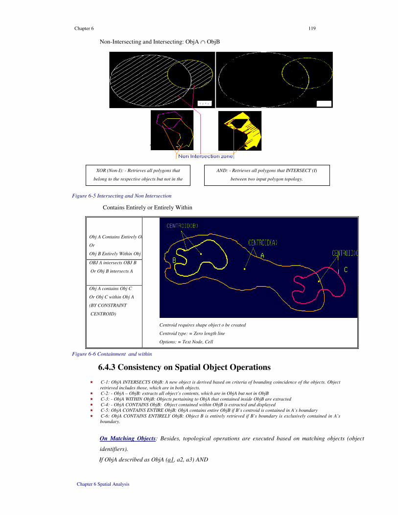
Chapter 6 119


Non-Intersecting and Intersecting: ObjA ∩ ObjB

Figure 6-5 Intersecting and Non Intersection

Contains Entirely or Entirely Within

Obj A Contains Entirely Obj B

Or

Obj B Entirely Within Obj A

OBJ A intersects OBJ B

Or Obj B intersects A

Obj A contains Obj C

Or Obj C within Obj A

(BY CONSTRAINT

CENTROID)

Centroid requires shape object o be created

Centroid type: = Zero length line

Options: = Text Node, Cell

Figure 6-6 Containment and within

6.4.3 Consistency on Spatial Object Operations

� C-1: ObjA INTERSECTS ObjB: A new object is derived based on criteria of bounding coincidence of the objects. Object

retrieved includes those, which are in both objects.

� C-2: - ObjA – ObjB: extracts all object’s contents, which are in ObjA but not in ObjB

� C-3: - ObjA WITHIN ObjB: Objects pertaining to ObjA that contained inside ObjB are extracted

� C-4: - ObjA CONTAINS ObjB: Object contained within ObjB is extracted and displayed

� C-5: ObjA CONTAINS ENTIRE ObjB: ObjA contains entire ObjB if B’s centroid is contained in A’s boundary

� C-6: ObjA CONTAINS ENTIRELY ObjB: Object B is entirely retrieved if B’s boundary is exclusively contained in A’s

boundary.

On Matching Objects: Besides, topological operations are executed based on matching objects (object

identifiers).

If ObjA described as ObjA (a1, a2, a3) AND

XOR (Non-I): - Retrieves all polygons that

belong to the respective objects but not in the

AND: - Retrieves all polygons that INTERSECT (I)

between two input polygon topology.

Chapter 6 120


ObjB described as ObjB (b1, b2, b3)

THEN ObjA.a1 = ObjB.b1

The Object is created based on the criteria of matching of the objects (rows) between the

objects.

The main difference between (contains and within) in one hand and CONTAIN ENTIRE and

ENTIRELY WITHIN is mainly due to the position of a centroid object and the status of a

bounded object, (i.e., one object encompassed within the other object) respectively. In the

absence of matching column, geographic objects are used to relate between two or more objects.

Both (object and matching field) techniques imply spatial analysis process in the form of attribute

and feature based spatial analysis. For instance it is possible to JOIN and extract the measurement

information related to MeasredHeavymetals object related to Geolithology Object composition as

indicated in the following formulation: -

MeasHeavymetals.OBJ WITHIN Geolithology.OBJ or Geolithology.OBJ CONTAINS MeasHeavymetals.OBJ

This shows that in an object relational GIS model, the communication among the objects is not

only based on matching numeric or textual attributes but also on objects that occur on both tables,

either as one object containing or intersecting the other.

6.4.4 Case Study: Object Relational Processes

Structurally, the Guayaquil zone is composed of NNW, NNE and E-W trend channels. The

estuary expands into the Gulf of Guayaquil, gets continental water supply from the perennial

rivers (see section 1.4.1) that flow to this partially enclosed body of water [17], [14].

Environmentally, the area is composed of distinct aquatic environment interfaces, extending from

the estuary-water-surface to estuary-bottom zone. This classification and the associated objects

are used to interpret spatially the environment of the estuary by employing certain statistical

tools.

6.4.5 Spatial Interpretation (SI)

The spatial analysis process includes objects of the multidisciplinary integrated coastal and main

estuary objects. Object relational Querying, Statistically classified thematical displays; overlay

and buffering based interpretations have been applied. However, before delving into detail, a

brief description of the statistical ranging process is given below.

Aggregation: Suppose one wants to present a thematic distribution of sediments (gravel, sand,

silt and clay) with respect to the measurement stations. The nature of the data is that a single

station is related not only to the x and y coordinates but also to the sampling depth in the same

station. In principle, one spatial object is supposed to be associated to one database record or

tuple. Then, how can this performed if the data format occurs as follows (see table 6-5)

Chapter 6 121


Table 6-5 Analysis Results table

A single station contains different informative database records. A centroid is assumed to be

associated to a database record, NOT records. A test on associating attribute records to spatial

features indicate the possibility of appending 80 database records to a single centroid feature in

(MicroStation Geographic) centroid, but to avoid unpredictable results the one to one

relationship is recommended in [11], [21], likewise a one to one join for the thematic mapping is

suggested [30]. Taking into account this natural occurrence of data, GIS applications are

equipped with aggregating functions.

Solution: - The multi-record-per-station nature of data shows that there are 180 records for the 25

stations. Thus, the data ought to be aggregated so that spatial feature with a specific geo-

referencing point fits to respective object (see table 6-6). For this purpose, a special SQL query is

designed.

1 TRANSFORM Avg (Results.pract_value) AS MeasValue

2 SELECT Location.station, Location.LonDegDec, LOCATION.LatDegDec,

3 Results.pract_unit AS MeasUnit, Field.environment, Field.discipline_name

4 FROM Location, field, Results

5 Where LOCATION.station = Field.station and

6 Field.field_code = Results.field_code

7 And Field.discipline_name = "SEDIMENTOLOGY"

8 GROUP BY Location.station, Field.environment

9 PIVOT Results.parameter;

Output

Table 6-6 Filtered Analysis Result table

Eventually, this output can be geo-referenced and appended. Appending of tabular data to objects

can be accomplished only if there is a relational cardinality of1111: 1 or∞∞∞∞: 1.

Chapter 6 122


6.4.5.1 Statistical Data Representation

Generating thematically visible GIS maps requires summarizing the geodatabase attribute values.

Main reason for this constraint is due to the 1: M cardinal relationships of a spatial object and the

attribute values. Aggregating process enable us to assign each value its own symbol or group the

values into classes applying different class for each symbol [89]. Therefore, classifying the bulk

database records enhances the impetus of thematically visible values in the map.

Values are classified statistically according to the distribution and this enables us to visualize

thematically the low, medium, high value pattern in the map. So if N = attribute database records

for a specific measured field parameter (MP) then range (R) for MP is: -

Max (N) – min (N) = R of MP

A representative class value: = (RCV or K = max (MP) – min (MP) / K

Table 6-7 Classfication Ranges

Figure 6-7 The Effect of Class Variation in Spatial Results display

Unique value mapping: Each unique value is symbolized with a different color. Drawing

features based on unique attribute values shows how different feature types are located in relation

to each other. This classification can also be used to sort the character typed attribute values.

Chapter 6 123


Standard deviation: The classification scheme depicts the amount a feature's attribute value

variation from the mean. A two or more color ramp could be used to mark out emphasis on

values above and below the mean. The mid range breaks at the mean of the data values, and the

ranges above and below the mid range is one standard deviation above or below the mean.

(a) Mean value, (b) classes above and below of (a) at Intervals of 1/4, 1/2, or 1 stdv

(c) Aggregates of any value beyond where the standard deviation is based on the formula:

Natural Break classification: The identification of the break points in natural classification

method is based on the identification of groupings and patterns inherent in the data (based on

Jenk’s optimization) This method is rather complex, but basically, the Jenk’s method minimizes

the sum of the variance within each of the classes. The features are divided into classes whose

boundaries are set to relatively big jumps in the data values. It minimizes the variation within

each class [21], because the range breaks are determined according to an algorithm such that the

difference between the data values and the average of the data values is minimized on a per range

basis [30]. A practical test on different number of classes from the same feature class (table)

shows different results. For instance, from a given object, taken higher number class will produce

an exaggerated distribution, view of graduated symbols; whereas a less number of classes will

show a restricted area distribution, viewed in graduated symbols. Despite the discrepancy of the

display that is due to the number of classes selected the spatial distribution lies within those

measurement or areas.

6.4.6 The Objects within Estuary and Coastal Periphery

A number of objects incorporated in the spatial analysis process include (a) MeasuredSed

object: Planned to comprehend sediments distribution and spatial affiliation to other discipline

parameters. Correlate the output with relevant objects in space and time.

(b) MeasuredBio object: Intended to decipher the spatial distribution of species. Differentiate

sites and zones biologically sensitive.

(c) MeasuredPhy-Chm object: planned to grasp the energetic water’s current and direction

variation and relate with phy-chm parameters (salinity, temperatures), spatial distributions

considerations of human and natural impacts in that coastal region.

(d) MeasuredChm object: intended to explain the spatial dissemination of chemicals and their

relationship with the sub marine environments.

(e) MeasureHeavyMetals Object: Aimed at understanding the magnitude heavy metals

dissemination across the estuary data mediums.

Chapter 6 124


(f) EstChannels Object: Objects that display the different parts of the estuary channels.

(g) GeoLithology object: Intended to explain the geo-setup, rock types and composition.

Interpret the associated lithologic parameters results and tectonics in the coastal area.

(h) GeoTectonics object: Intended to assess the geo-tectonic trends of the estuary channels and

shearing Lithology of the coastal zone.

6.4.7 Object Relational Spatial Analysis

6.4.7.1 Problems and Solutions

Two objects (HeavyMetals and EstChannels) are involved. The HeavyMetals object is of Point

type representing measurements sites whereas the EstChannels are the main parts of the estuary

water body. The retrieving and visualization incorporates Object-Relational query, spatial and

logical operators and aggregate functions.

6.4.7.2 Objects: HeavyMetals vs. EstChannels

Find and display part of the estuary that shows higher measured values of cadmium than mercury

(mg/kg).

1 SELECT *

2 FROM EstChannelaObject, HeavyMetalsObject.mercury

3 WHERE EstChannelsobject.obj

4 CONTAINS HeavyMetalsObject.obj

5 AND HeavyMetalsObj.cadmium > HeavyMetalsObj.mercury

Figure 6-8 Output (Light blue) cadmium greater than mercury (mg/kg)

Output reveals that the southern channel is characterized by a low dissemination of Hg.

6.4.7.3 Objects: GeoLitho_region, Sediments Object

Find and display the distribution of sediments confined within specific Lithology type.

� SELECT * From GeoLitho_region, Sediments

� WHERE GeoLitho_region.obj Contains Entire SEDIMENTS.obj

� And Sediment.sandpercent > sediment.gravelPercent ;

The output of the spatial query is:-

Chapter 6 125


Figure 6-9 Lithology containing MeasPoints and Sand>Gravel(%)

6.4.7.4 Objects: GeoLitho_region and GeoTect_polyline

Problem:

What is the dominant Geolithologic composition (GeolithObject), which is strongly sheared by NW

fault direction? - Identifying highly sheared, composition and trend. First step is to formulate the query

as follows>


Chapter 6 126


Figure 6-10 North Westerly Sheared Geolithology

The spatial process retrieves the Lithology extension, lithologic contact to the main estuary and

sheared zone with trends mainly to the NW direction.

6.4.7.5 Objects: GeoLithology, GeoTectonics and MeaResults

The following spatial query extracts all the information in the three objects GeoLithology,

GeoTectonics and MeaResults. The GeoLithology in the coastal area that is sheared by

Geotectonic structures trending East-West direction and relates to the sites which contains

maximum of silt% range between 60 and 80.

Problems and Solutions

Find and display the area dissected by E-W trending fault lines, maximum silt% ranging between 60 and 80 and

the depth sampling between 1 and 10 m.

•••• Select *

•••• FROM GeoTect_polyline, GeoLitho_region, MeaResults

•••• WHERE GeoTect_polyline.obj INTERSECTS GeoLitho_region.obj

•••• AND GeoLitho_region. LithID = MeasResults.MSLINK

•••• AND GeoTect_polyline. FTDESC LIKE "%E-W" And

•••• MeasResults.MAX (SILTPERC) BETWEEN 60 AND 80

•••• AND MeasResults.maxdepth BETWEEN 1 AND 10 ;


Chapter 6 127


Figure 6-11 East – West dissecting faults

6.4.8 Coastal Area Spatial Analysis

Problem: finding the spatial information heavy metals distribution associated with tectonically

sheared zone. Interacting objects are GeoLithology and GeoTectonics Objects and HeavyMetals.

It does the followings.

• Step 1: Find and retrieve the geolithology dissected by GeoTectonics trending E-W.

• Step 2 retrieve the geolithology description that sheared by this trend.

• Step 3 retrieves and display in a pie chart the concentration of heavy metals that meets the criteria stated in step1

and step 2; i.e., a lithology dissected by E-W faults and contains measurement sites related to the heavy metals

dissemination.

6.4.8.1 Geolithology and GeoTectonics

GeoLithology (Region or polygons)

Step 1.

1 SELECT *

2 From GeoLitho_region, GeoTect_polyline

3 Where GeoLitho_region.obj Contains GeoTect_polyline.obj

4 and GeoTect_polyline. FTDESC = "EW"

GeoTectonics (Polylines) Step 2

1 SELECT *

2 From GeoTect_polyline.obj, GeoLitho_region

3 Where GeoTect_polyline.obj INTERSECTS GeoLitho_region.obj

4 And GeoTect_polyline. FTDESC = "EW"

GeoLithology + GeoTectonic and HeavyMetals (measurement point info within region) STEP 3

1 SELECT *

2 HeavyMetals, GeoLitho_region, GeoTect_polyline

3 WHERE HeavyMetal.obj Entirely Within GeoLitho_region.obj

4 and GeoLitho_region.obj Contains GeoTect_polyline.obj

5 and GeoTect_polyline. FTDESC = "EW"

Chapter 6 128



Figure 6-12 Distribution of Cu-Zn-Pb, associated thematical Geology and GeoTectonics

The thematical display performed by relating relevant objects of the measurement results,

GeoLithology and GeoTectonics disclose that the major fault trending NS and NW dissect the

different Lithologies in the coast (see figure 6-11). The sheared zone that extends southwards

appears to have effect on the structure of the estuary.

Moreover, the HeavyMetals object thematic pie distribution shows higher zinc distribution

(heavy metal) throughout the estuary than copper and lead (Pb).

The NW trending faults, close to the estuary flanks could have certain clue of mineralized

solutions (sulfide) [16] that influence the concentration of the measured higher base metals,

specially the zinc.

Furthermore, the description of the rocks indicates some pyrite and malachite rich outcrops,

which support the possibility of mineralization along these fractures.

Despite the restricted data applied, this spatial analysis based hypothesis suggests a hint that in

addition to the possible human impact, the origin to the measured higher concentration of Zinc

could be attributed to the discharge of a sub-volcanic mineralized solution associated to shearing

process close to the estuary.

Chapter 6 129


6.4.9 Thematic Correlation

The thematic distribution pattern of the heavy metals shows variability.

Figure 6-13 Correlated Pie thematic map of Zn,Pb and Pb

A comparison across different estuary measurement mediums (bottom sediment, bottom water

and surface water), disclosed in figures 6-13 and 6-14, shows that Bottom sediments environment

is characterized by relatively higher dissemination of Zn than Pb and Cu respectively.

FFigu

re 6-14 Correlative Environmental Distribution of Heavy Metals

E n v iro n m e n t v s . H e a v y M e ta ls D is tr ib u t io n

0

2 0

4 0

6 0

8 0

1 0 0

1 2 0S S S S S S S S S S S S S S S S S S S S S S S S B B B B B B B B B B B B B B B B B B B B B B B B B S S S S S S S S S S S S S S S S S S S S S S S S

E s t u a r y E n v i r o n m e n t

Mic

gm

/l

c o p p e r le a d zin c

S u rfa c e W a te r E n vi ro n m e n t B o tto m W a te r c o lu m n E n vi ro n m e n t B o tto m s e d im e n ts E n vi ro n m e n t

Chapter 6 130


6.4.10 Buffering - on Relevant Criteria

A buffer is created as concentric rings or measured specified distance from geographic

features(s). The objects can be points, polylines or polygons.

Buffers are useful for the purpose of proximity or nearness analysis in area where geographic

features are constructed for the performances of spatial analysis. (For example, finding

measurement points within 500 meters of a proposed sheared zone).

For a point type object the point value can be either of Spherical or Cartesian x, y coordinates.

The size of the buffer depends on the defined radius of the object in a specific unit. Using

Latitude/Longitude data, the perfect buffer width, as defined in native Latitude/Longitude

decimal degrees, may change on different portions of an object. This is because the width

provided is in somehow flat measurement unit, (e.g. miles, meters), and the decimal degree to

measurement transformation will vary depending on the location on the earth. For instance, a

kilometer spans a larger number of latitude degrees as one move toward the poles of the earth and

away from the equator. On small objects, the distance may be negligible. Buffering point type

objects, in an area where they are scarcely populated, requires larger radius to generate an outline

or rings around the objects. For instance, two point objects, 6 km apart can be buffered wholly by

a radius a little greater than half distance (D), between them, see figure 6-15. Furthermore, the

tabular information of the buffered polygon object is reported with the shape length, shape area

and distance intervals, see table.

Table 6-8 Buffer Class Ranges

During geographic element buffering, any object residing with a radius less than the distance

between two points is included within the buffer zone. Specifying the desired distance from the

polyline type object can also perform buffering.

Figure 6-15 Buffered Points and Zone Generated

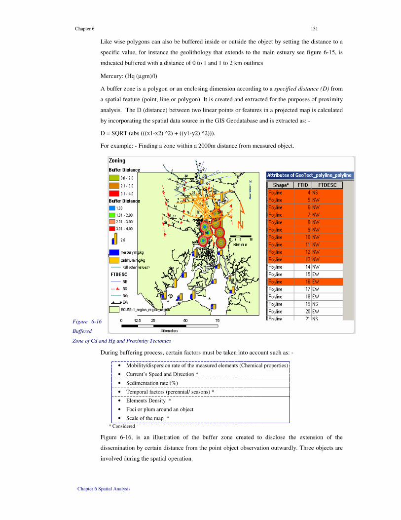
Chapter 6 131


Like wise polygons can also be buffered inside or outside the object by setting the distance to a

specific value, for instance the geolithology that extends to the main estuary see figure 6-15, is

indicated buffered with a distance of 0 to 1 and 1 to 2 km outlines

Mercury: (Hq (µgm)/l)

A buffer zone is a polygon or an enclosing dimension according to a specified distance (D) from

a spatial feature (point, line or polygon). It is created and extracted for the purposes of proximity

analysis. The D (distance) between two linear points or features in a projected map is calculated

by incorporating the spatial data source in the GIS Geodatabase and is extracted as: -

D = SQRT (abs (((x1-x2) ^2) + ((y1-y2) ^2))).

For example: - Finding a zone within a 2000m distance from measured object.

Figure 6-16

Buffered

Zone of Cd and Hg and Proximity Tectonics

During buffering process, certain factors must be taken into account such as: -

• Mobility/dispersion rate of the measured elements (Chemical properties)

• Current’s Speed and Direction *

• Sedimentation rate (%)

• Temporal factors (perennial/ seasons) *

• Elements Density *

• Foci or plum around an object

• Scale of the map *

* Considered

Figure 6-16, is an illustration of the buffer zone created to disclose the extension of the

dissemination by certain distance from the point object observation outwardly. Three objects are

involved during the spatial operation.

Chapter 6 132


(A) The GeoTectonic (NW and NS fault alignments), (B) HeavyMetals object: (A bar thematic

charted dissemination of Cd and Hg) and (C) The coastline features.

A spatial query on retrieving the geotectonic trending NW and EW are selected and thematically

viewed. The NW structures alignment coincides with the northern part of the eastern channel.

Furthermore, the NS and NW trending fault lines indicates the presence of catchments that flow

towards the estuary with possible; mineralized solutions that dilute the estuary water body,

Concentration of Mercury and Cadmium displayed by means of bar chart type is characterized

by elevated distribution of the elements in the northern part of the estuary.

Figure

6-17

Estuary

Water

Temperature and Salinity

The buffering process (two regions), in the North West and North East, shows zones with

maximum concentration distribution of mercury Hq (µgm) /l, (see figure 6-14). Applying a one

km interval (bounded zone), the zone with the maximum concentration coincides along the

southerly extending sheared zone or fault line (see figure 6-16), suggesting the effect of and

influence geodynamic processes and the also possible effect of human activities.

6.4.10.1 Salinity and Temperature

Temperature and Salinity: The measured water temperature ranging 25.2 to 26 is higher, close to

continental terrain, which is rather a normal phenomenon when contrasted to the seaward

temperature. On the other hand, the southern zone is characterized by colder (symbolized by

green color) temperature ranging 24 to 24.6 Celsius. This zone is close to the outlet of the estuary

to the ocean.

The colder temperature is attributed to the cold-water current surge and swelling of colder current

from the sea to wards the estuary, at the period of measurement. Otherwise, salinity is higher

towards the ocean compared to the depleted salinity landwards (see figure 6_17).

Chapter 6 133


6.4.10.2 Sediments and HeavyMetals

An attempt was also done to spatially analyze the relative relationship of the clay% standard

distribution with the heavy metal Mercury (Hg, mg/kg) standard deviation distribution along the

estuary’s measurement stations. There is a positive relationship between the clay and mercury

for values calculated close to the 1.5 stdv. The graduated symbolization shows that stations with

higher mercury also display similarity in distribution of clay%. Furthermore, such relationship

indicates that clay rich sediments are vulnerable to the effect of mercury contamination. The

higher value of the clay corresponds to the higher values of mercury, suggesting that there is

higher affinity of the mercury dissemination with distribution of clay. Such relationship indicates

that clay rich sediments are vulnerable to effect of mercury contamination. To verify the area,

buffer zones were created around the anomalous features, indicated as Z1 (Zone 1) and Z2 (zone

2), (see figure 6-18), polluted (stations 18, 19, 20) is close to activity zone with meandering and

relatively narrow stream tributaries whereas, Z2 (station 11 and 12) is adjacent to environ

prevailing a human activity zone. There are signs of elevated Hg, (kg/mg) in the north-eastern

channels (station 5, 6), which were beneath coverage of a 1 km buffer zoning.

Figure 6-18 The

standard deviation distribution of Clay and Mercury

6.4.10.3 Overlay Interpretations

Based on overlay spatial interpretation mechanisms, i.e., superimposing satellite image map and

vector features, it was possible to disclose impacts of activities. These effects were thematically

Chapter 6 134


visualized close to the southern periphery of the estuary and regions under submarine erosion

pressure, (see figure 6-19).

The process deciphered that the southern island’s northern flank (resymbolised red color)) is

deeply dissected and a canyon is being created. This may facilitate an early failure of the

unconsolidated coastal sediments. Moreover, close up view of the spatial overlay, of thematic

viewed maps suggest that southern part of the main estuary land is pinching out southwestward

(see figure 6-19), most probably due to submarine erosion impact.

These evidences rounded up from the spatial overlay analysis imply that the dimension of the

southwest estuary water body is expected to extend further northwards and the southern island

might submerge as a repercussion of combined effects of human and nature dynamism.

Figure 6-19 Submarine Processes and effects

6.4.11 Meta Data (MD)

6.4.11.1 Managing Meta Data

In the domain of GIS, Meta Data is advantageous in describing and understanding more an

associated geographic object. Meta data are created as Hyperlinks or hot link types with a

required full or relative path before being utilized. For instance D:\AMAPIFO2K44\CORE.BMP"

Chapter 6 135


is an image of .bmp type pointing to the root D. The Meta data variable (field) is of text type and

the string path is the value stored and associated with the object. It inherits the object Identifier

that describes it uniquely within Geodatabase system. The textual value of the Meta data attribute

is retrieved by means of object querying methodology.

The examples below show the process of creating and managing core and video Meta data type

associated to a respective object. The object is created within the Geodatabase; a separate field is

established (for storage) for the Meta data path associatable with an object. The implementation

is based on [37] and the attribute database is stored in .mdb.

Geodatabase Definition Table: = “equx.mdb"

Type ACCESS TABLE/ object "BioOrgAbundance"

a. Step 1: Fields 20

b. MSLINK Integer;

c. Mapid Integer;

d. Station Char (25);

e. Area Float;

f. Perimeter Float;

g. Step 2:

h. Video Path Char (100);

i. CorePath char (100);

j. Step 3: Path Pointer k. Begin metadata

l. "\ActiveObject" = ""

m. "\ActiveObject\Expr" = "Video"

n. "\ActiveObject\Mode" = "HOTLINK_MODE_BOTH"

o. "\ActiveObject\Relative" = "TRUE"

p. "\IsReadOnly" = "FALSE"

q. End_metadata

r. Begin_metadata

s. "\ActiveObject" = ""

t. "\ActiveObject\Expr" = "Core"

u. "\ActiveObject\Mode" = "HOTLINK_MODE_BOTH"

v. "\ActiveObject\Relative" = "TRUE"

w. "\IsReadOnly" = "FALSE"

x. End_metadata

Object relational spatial queries can retrieve Meta data (images, documents, videos and audio)

integrated with specific spatial objects. .

6.4.11.2 Retrieving Approaches (Raster Type)

The MeasSediment Object is described by its geospatial set of data source and the measured

attribute values pertaining to Sedimentology discipline. However, there exist additional data

about the MeasSediment spatial feature. These are core samples showing the physical nature of

the data, stored in a separate space but integrated to the specific object as a Meta data. Two

objects (MeasSediment and the EstChannels) are involved in the process of retrieving and

visualizing the Meta data.

See retrieval steps below: -

Step 1

1 SELECT

2 SEDIMENTS, EstChannels ‘ two objects

3 Where EstChannels.Obj Contains Sediments.Obj ‘ first object contains second

4 And SEDIMENTS.CORE1 = "D:\AMAPIFO2K44\CORE.BMP" ‘pointer to core path

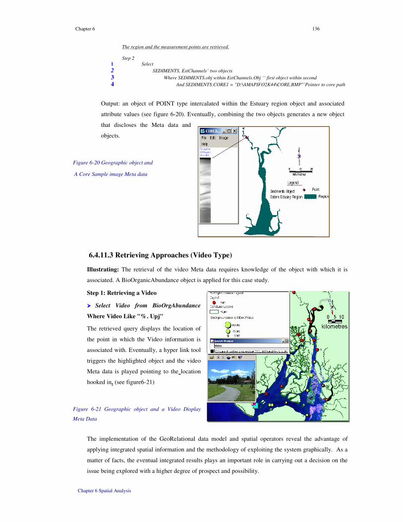
Chapter 6 136


The region and the measurement points are retrieved.

Step 2

1 Select

2 SEDIMENTS, EstChannels ‘ two objects

3 Where SEDIMENTS.obj within EstChannels.Obj ‘‘ first object within second

4 And SEDIMENTS.CORE1 = "D:\AMAPIFO2K44\CORE.BMP"’Pointer to core path

Output: an object of POINT type intercalated within the Estuary region object and associated

attribute values (see figure 6-20). Eventually, combining the two objects generates a new object

that discloses the Meta data and

objects.

Figure 6-20 Geographic object and

A Core Sample image Meta data

6.4.11.3 Retrieving Approaches (Video Type)

Illustrating: The retrieval of the video Meta data requires knowledge of the object with which it is

associated. A BioOrganicAbundance object is applied for this case study.

Step 1: Retrieving a Video

�� Select Video from BioOrgAbundance

Where Video Like "%. Upj"

The retrieved query displays the location of

the point in which the Video information is

associated with. Eventually, a hyper link tool

triggers the highlighted object and the video

Meta data is played pointing to the location

hooked in. (see figure6-21)

Figure 6-21 Geographic object and a Video Display

Meta Data

The implementation of the GeoRelational data model and spatial operators reveal the advantage of

applying integrated spatial information and the methodology of exploiting the system graphically. As a

matter of facts, the eventual integrated results plays an important role in carrying out a decision on the

issue being explored with a higher degree of prospect and possibility.

Chapter 6 137


6.5. Results and Conclusions

� Overlay analysis interpretations of the interdisciplinary objects have been carried out by

implementing object-relational analytical methodology

� Interoperability of features among different GIS applications and the Georelational model has

been executed via SQL and ODBC connections. One of the interoperability processes includes -

translating features type specific to a spatial engine. The output of the test disclosed preservation

and loss of features properties on non OPEN GIS complaint applications.

� A Hybrid of Object Relational spatial operators and SQL statements were constructed to perform

spatial search and display thematical information. The process has been accomplished by

executing the required topological relationship, checking containment of the spatial features,

georeferencing compatibility of the geographic objects and creating migrating spatial pointers

among the objects.

� A methodology of integrating and retrieving Meta Data associated with geographic objects has

been developed. The output revealed the possibility of utilizing objects and object relational

operators to retrieve and display full-fledged Meta data spatial information of such as video, audio,

image and documents that further elaborates the results of the spatial interpretation.

� Implementation of the Georelational GIS data model carried out in the Guayaquil estuary GIS

case study reveals zones of contaminated sediments, anomalous affinity of heavy metals to

sediments (clay); indicating that clay rich sediments are conducive medium to mercury deposition.

� Buffering process of the point type objects shows that the northeast and north west of the estuary

are characterized by higher concentration of mercury and that zone coincides with the southerly

extending shear zone, indicating geodynamic effects in addition to the human impacts.

� Comparison of surface water, bottom water and Bottom sediments environment revealed that the

surface water is characterized by relatively higher dissemination of Cd than Hg.

� An interpretation of the satellite image and vectorised features (southern part of the estuary)

discloses the presence of unstable submarine zones as a repercussion of human and submarine

erosion process.

Chapter 138

Chapter 7: Spatio-temporal Analysis

Chapter 7: Spatio -Temporal Analysis

7.1. Introduction In the field of location based geosciences, GIS, is composed of space, time and attribute components.

Connected with this, at the phase of a spatial analysis, a set of geometry-based spatial objects are

applied to represent thematic reality using different symbols with respect to classified time intervals.

In this work, the main spatio-temporal analysis focuses on the current velocity and direction in the

Guayaquil estuary. Furthermore, an extended theoretical explanatory aspect on the causes of tide

generating forces and possible influence on the nature of the current’s velocity and direction is

encompassed within the chapter. With this regard, the core theme concentrates on exploring the

possible ways of processing and analyzing spatio-temporal data in a coastal marine environment GIS.

Moreover, it emphasizes the analysis intended to extract and visualize environmental phenomenon in

a spatio-temporal perspectives and the importance of tracking and processing of a real-world time

elapsed ever since an event had been in the process in order to manage and predict about future

changes. Henceforth, a brief description on temporal concepts in relation to spatial sciences is given,

pursued by the theoretical aspects on the causes of tides and processes of spatio-temporal

implementation of the Geodatabase GIS.

7.2: Spatio -Temporal Conception In spatial science, the temporal information is associated with

time-stamped individual layers, which can be explained as the

temporal map set (TMS) [85], (see Figure 7-1 and snapshot models

[86]. In the snapshot model, every layer is a collection of

temporally homogeneous units of one theme. It shows the states of

a geographic distribution at different times without explicit

temporal relations among layers.

Figure 7- 1: TMS Model (after Beller et, 1991)

The fact that location based information is dependent on time, implies that, a location can’t exist

without a time (t) and remain always-interconnected issues. It implies that both spatial and temporal

references are required to define a location. The design of TMS endeavors to model geographic

Chapter 139


events in a defined area. The major drawback is its data redundancy and the risk of data

inconsistency [88].

On the other hand, the Space -Time Composites (STC) model represents the world as a set of

spatially homogenous and temporally uniform objects [87] in 2D space (see Figure7-2). The space-

time composites can be derived by temporal overlays of time-stamped layers (snapshots) and attribute

changes are recorded at discrete times.

Figure 7- 2: An example of an STC layer for burns

(Modified from Lnagran and Chrisman, 1988)

The STC model enables to record

temporality within the largest common units

of attribute, space, and time (i.e. change in

situ), but according to [87] this model fails to

capture temporality among attributes across

space (i.e., in motion or movement).

7.2.1 Spatio-Temporal Processes

7.2.1.1 Spatio-Temporal Significance

Incorporating temporal analysis of data in GIS is vital for a number of logical reasons: -

Every event and process that occurs on the earth’s data happens through a chain of time spans; and

most data are subjected into different transforming processes either pre or post measurements.

Therefore, as a function of time (F (t), attributes compositional variations can be gauged. Example, a

steady dynamic fluctuation of the coastal process through time results in reshaping the coastal

morphology and changes the habitat of the ecosystem.

As an illustration of the process, in the coastal zone, the study of current mobility and direction

allows us understanding and interpreting maps in the form of category time_t_map, category

time_t+1_ map, category time_t+2_ map …etc.

Chapter 140


7.2.1.2 Spatio-temporal Analysis Process (STA)

A.

t1, t2, t3

O

time

spatialobj.

adr.

R1

R2

R3

The purpose of such STA is to associate informative attributes values and temporal marker data with

their respective geo-referenceable geographic features (see figure 7-3). The factors described as Dim

1, Dim2, Dim3 and Dim4 (see figure 7-4) represent a geographic element, time stamp, measured

informative attribute values and aggregated values respectively. As spatio-temporal information is

information indexed with time [40], then the issue of thematic display becomes complex; especially

when multiple attribute records are not only referenced to two dimension features (point, line) but

also to time-stamp component of the

geodatabase.

Figure 7- 3: Spatio-Temporal Retrieval Cycle

At this juncture, the need of aggregating

process (see figure 7-3) crops out and is carried out to establish correspondence between associated

database records (D3) and specific spatial object (D1) tagged to specific date and time (D2), (see

figure 7-4).

Thus, temporal queries have been incorporated to enable smooth search of possible answers

pertaining to what had happened, is happening and would happen along geo-reference able sites

through time.

Thus, for instance, if a regularly measured temperature gradient is increasing gradually from time-1 to

time-2 and the influencing factors are outlined; it might be possible to establish a possible model that

help to predict and project the phenomenon in a geo-referenced time-n. To enact it, additional

availability of elapsed period’s measurements is prerequisite. It is possible to incorporate influencing

factors (seasonal, global climate changes and human activities impact) such as ELNINO [15], which

influence the climate variation in the Gulf of Guayaquil (Guayaquil estuary).

7.2.1.3 Composing Spatio-temporally

Normally, a geographic object occurs uniquely in a specific geodatabase system. But, some times a

single spatial object can be related to other attribute database records (adr.), linked to different

Temporal attributes (see figure 7-3). This would rather create a relationship of I: M type where a

geographic element is related to many attribute records and this contradicts the principle of 1:1

mapping. In such conditions the natural relationship between a spatial object and the attribute

database records (adr.), in a 2D GIS, results in producing a number of information layers represented

by different symbols to represent the evolution of a single parameter values through time. Referring

Chapter 141


to figure 7-4, the Dim 1 (dimension) represents the spatial object coordinate that is described by Dim

2 (temporal attributes) pertaining to alphanumeric attributes (Dim 3).

Any change in the magnitude of dim 3 as F(t) should be reflected in the change of spatial object

(dim1). The point is that the spatial object should respond to changes that occur in Dim 3 via Dim 2

to indicate that spatial objects are also dynamic.

Figure 7-4: Spatio-

Temporal data processing

Otherwise, Dim 3 data

should be aggregated

with specific time

such that as F (t) and F

(R1 to R1+n) then an

aggregate (A) that

corresponds to a spatial object is generated, (see figure 7-4). On the temporal dimension could not be

aggregated because it represents a specific temporal event in the system that can’t roll back. Hence, a

roll back operation cannot be committed is ruled out.

In the case of a single spatial object S where (S1=S2= S3=S4 …) S=S1 to Sn, the spatio-temporal

analysis can only be carried out by creating different Spatio-Temporal Layers (STLs) that correspond

to Dim 3, or adr, (See figures 7-5), and this process of can be explained as follows.

For the L1 = layer 1, L2 = layer 2: R1, R2 records, at x, y, t

L1 = corresponds to S1 & R1 at time t1

L2 = corresponds to S2 & R2 at time 2: where S1 =S2

In a multiple dimensions, (Dim 1, Dim 2,) which are represented by (S=S1-Sn) and (T=T1-Tn)

respectively, the possible spatio-temporal layers (STLs) can be retrieved by changing relationship

between the spatial object and time to M: 1 respectively.

To retrieve and symbolize information related to the question what happen in different geographic

locations at a particular time.

Thus: -For 2D geographic objects:

L1= X, Y related to R1 tagged to t1 = X, Y: R1T1

L2= X, Y related to R2 tagged to t2 = X, Y: R2T2

If the x, y of L1 = x, y for L2 the spatio-temporally tagged data is symbolized once at a time.

Chapter 142


For 3D geographic objects:

L1= X, Y, Z related to R1 tagged to t1 = X, Y, and Z: R1T1

L2= X, Y, Z related to R2 tagged to t2 = X, Y, and Z: R2T2

Based on this spatio-temporal relationship, the objects thematical resymbolisation is performed

discretely.

------------------------------------------------------------------------------------------------------------------

Figure 7- 5: (A) Multiple Spatial Objects at Time1 (t1) (B) Changes R to R1+1 in S1 as F (t])

Chapter 143


The layer information (L1), (see figure 7-5 A) is the output of the combined spatio-temporal and

associated informative database records, ranging from record1 (R1) to record6 (R6) constrained with

specific time filter. Further, layers of information are derived in the same pattern for (T=T1 to Tn)

and geographic features (S=S1 to Sn) for any event that occurs through time in different geo-

referenceable observation points.

The possible changes on an associated attribute values, on a specific site and a sequence of time

includes -

At Time (t1), L1 = is described by R1S1 (attributes assimilation to unique geographic element)

At Time (t2), L2 = is described by R2S1 = At Time (TN+1) Ln = is described by RnSn

The changes on the associated attribute values, as a function of time are distinguished using different

symbols.

Such phenomenon can be illustrated by the changes of attribute composition recorded in a specific

geo-referencing point at different times.

For instance at time T, concatenated to a specific LL coordinate, the attribute (for instance sediment

composition) value transition of grain size can be described as silty at time 1 and can be gauged at T

(i+1) as sandy, depending on events that took place during T (i+1).

Chapter 144


Figure 7- 6: Spatio-temporal effects on attribute components

Moreover, the situation may also be described as gravelly composition at T (i+2), depending on the

grain size changes of the sediments, as schematically illustrated (see figure 7-6).

7.3: The Causes of Tides: A Theoretical Aspect Daily, ocean water intrudes the shorelines to flood bays and estuaries. It inundates mud flats and

marshes, raises the water levels, and surges landward with sufficient force. As the process continues,

salt water mingles with fresh water, and within hours, the brackish brew slackens briefly to deposit

valuable nutrients that feed countless organisms residing in coastal waters or in the complex estuarine

system. Then, the process reverses, and receding waters flush the estuary, carrying organics and

inorganic materials and even potentially harmful pollutants to the sea.

These predictable and periodic movements of ocean waters are known as tides and are caused by the

attractive forces of the moon and the sun. Sir Isaac Newton’s law of gravitation tells us that any two

bodies in the universe are attracted to each other and that strength of this attraction depends on the

bodies’ mass and distance from each other [103].

The sun’s mass is greater than that of the moon but also the distance is further from the earth in

contrast to the moon. Therefore, although the sun affects the tides, the moon exerts greater

gravitational attraction because of its proximity to our planet.

Besides, the great variety of the earth’s topography, as well as other terrestrial influences causes the

tides to differ in various ways and exhibit certain similarity. Along the coasts, tides can vary greatly,

depending on the topography and other influences. In some parts of the world, the range of the tides is

Chapter 145


measured in inches; elsewhere, the disparity can be dramatic. At the Bay of Fund, in Nova Scotia, for

example, the difference between high and low waters can be as much as 15m [103] whereas in the

Guayaquil estuary the tidal ranges 3 to 5 meters [96].

7.3.1 Definition

The word “tides” is a generic term used to define the periodic rise and fall of the sea level with

respect to the land, produced by the gravitational attraction of the moon and the sun [104]. In other

words, it is astronomically induced vertical change in the height of the sea surface caused by slight

variations in gravitational attraction between the Earth, the moon and the sun [105] and geometric

relationship with locations on the Earth's surface [106].

The moon is the primary factor controlling the temporal rhythm and height of tides. The moon

produces two tidal bulges somewhere on the Earth through the effects of gravitational attraction. The

height of these tidal bulges is controlled by the moon's gravitational force and the Earth's gravity

pulling of the water back toward itself.

The second factor controlling tides on the Earth's surface is the sun's gravity. The height of the

average solar tide is about 50 % the average lunar tide [112]. At certain times during the moon's

revolution around the Earth, the direction of its gravitational attraction is aligned with the sun's

gravitational force. According to [106], at location on the Earth closest to the moon, seawater is

drawn toward the moon because of the greater strength of gravitational attraction. On the opposite

side of the Earth, another tidal bulge is produced away from the moon (due to the fact that at this

point on the Earth the force of the moon's gravity is at its weakest). Considering this information, any

given point on the Earth's surface should experience two tidal crests and two tidal troughs during each

tidal period (figure 7-7).

Knowledge of the times, heights and event of inflow and outflow of tidal waters is of significant

importance in a wide range of practical applications such as in: navigation through intracoastal

waterways, within estuaries, bays and harbors, establishment of standard datum, and furnishing of

data indispensable to fishing …etc and other considerable related issues.

7.3.2 Tidal Ranges Fluctuation

Currents reflect the horizontal movement of water, whereas tides reflect vertical movements. This

movement is primarily caused by the gravitational pull of celestial bodies and other factors playing a

significant role include - differences in water temperatures, differences in salinity caused by rain,

evaporation and friction … etc. Thus, tides are vertical rise and fall of the surface of water caused

http://www.physicalgeography.net/physgeoglos/g.html#anchor510801

Chapter 146


primarily by the differences in gravitational attraction of the moon, and to a lesser extent the sun,

when the positions of the moon and sun change with respect to the earth. The process results in

generating different types of tides such as the spring and neap tides...

Spring tide occurs when the sun, earth and moon are aligned straight with a tide larger than average.

On the other hand, the Neap tide occurs (smaller than average) average [100], when the moon is at

right angles to the earth-sun line.

The effects of landmasses, constrained waterways, friction, may distort this basic pattern … etc. The

incoming tide along the coast and into the bays and estuaries is the flood tide and the outgoing is the

ebb tide. As the tide rises, water moves towards the shore (flood current) and as it recedes moves

away from the shore (ebb current), (see figure 7-7).

Figure 7- 7: The flood and Ebb

Tidal Ranges

In the open ocean, tidal currents are relatively weak. Near estuary entrances, narrow straits and inlets,

the speed of the currents can reach up to several kilometers per hour [111], but it can be slowed by

friction against the bottom of the ocean.

These dynamic aspects of tides result in variation of the number of highs and lows per day at different

locations.

Therefore, even though the forces that move the tide are well understood, the tides at any spot are

essentially impossible to calculate theoretically, [113].

What we can do is to record the height of the tide at that spot over a certain period, and use these

measurements to predict the tides in the future.

Chapter

147

7.3.3 How are they created?

7.3.3.1 Positional Effects

Understanding how a tide forms require considering, that, the pull of the moon is slightly stronger on

the side facing the earth. This causes the earth to elongate slightly towards the moon, and due to

reason that water is more flexible than rocks, most of stretching occurs on oceans. This raises a small

tidal bulge on the earth facing the moon and on the opposite sides of the earth, (sees figure 7-11). The

timing of these tidal events is related to the Earth's rotation and the revolution of the moon around the

earth. One revolution takes about 27 days and adds up about 50 minutes to the tidal cycle [107],

[108].

As a result, the tidal period (Time it takes for one tidal cycle) is 24 hours and 50 minutes in length.

The tides at a given place in the Earth's oceans occur about an hour later each day. These situations

are explained with respect to the positional phases of the moon known as the syzygy and quadrature,

[106] (see figure 7-8).

The gravitational attractions (and resultant tidal

force envelopes) produced by the Moon and Sun

reinforce each other at times of new and full

moon to increase the range of the tides, and

counteract each other at the first and third

quarters to reduce the tidal range, (see figure 7-

8). The variation of tides can be explained as

follows.

Figure 7- 8: The Phase Inequality: Spring and Neap Tides

Quadrature: When the moon is at first and third-quarter phase (quadrature, perpendicular position to

the sun), the gravitational attraction of the moon and the sun upon the water of the earth are exerted at

right angles and relatively small tidal ranges, known as neap tides generated.

Syzygy: When the moon is at new and full phase (syzygy), the gravitational attraction of the moon

and the sun align to act and reinforce each other. Thus, the resultant tidal force is also increased; the

observed high tides are higher. Such greater-than-average tides resulting at the syzygy position of the

moon are known as spring tides; a term indicating welling up of the water or short-period,

astronomically induced vertical change in the height of the sea surface, [104], (and 7-12).


http://www.physicalgeography.net/physgeoglos/t.html#anchor1774028

javascript:locscrollmenu('http://www1.pactide.noaa.gov/information.htm','tides',650,450)

Chapter 148


7.3.3.2 Parallel effects

Since the moon follows an elliptical path, the distance between the moon and the earth will vary

throughout the month. The Moon exerts a gravitational force on every object on and in the Earth.

Some parts of the Earth are closer to the Moon than other parts, and since the gravitational force

drops off as the inverse square distance [108], those parts closer experience a larger gravitational tug

from the Moon than parts that are further away [109].

According to [108], Every object in the universe attracts every other object with a force directed

along the line of centers for the two objects that is proportional to the product of the masses and

inversely proportional to the square of the separation between the two objects (i.e., Law of universal

gravitation) is defined by: -

Where Fg is the gravitational

force, G is universal gravitational

constant, m1 and m2 are the

masses of the two objects and r is

the separation between the two objects. Thus, the distance is a function of the mass attracting forces

and any change of it will influence the force of gravity being exerted on the earth surface there by

influencing the nature of the tides range. For instance changing the d2 towards left will shift the

center of mass towards m1 to keep the center of mass in balance and vv, (see figure 7-9).

m1d1 = m2d2 and d1 + d2 = d (ly)

d1 = [m2/(m1 + m2)] d

d2 = [m1/(m1+m2)] d

Figure 7- 9: The Center of mass

With this regard, once a month when the earth orbit

is closest to the moon’s orbit (perigee), [104], the

tide generating force will be higher than usual, thus

producing more than-average-tide ranges. Conversely, about two weeks later when the moon is at the

farthest (apogee) from the earth, the lunar tide raising force will be lower and the tide ranges will be

below average. Similarly, in the earth-sun system, at the perihelion (sun’s closest position to the

earth,) and aphelion (sun’s furthest position), the tidal range will be enhanced and reduced

respectively, (see figure 7-10).

The fluctuating tidal heights and the changing of current direction as well as in speed are mainly the

result of the fluctuating gravitational forces of sun and moon on the water masses of the earth [107].

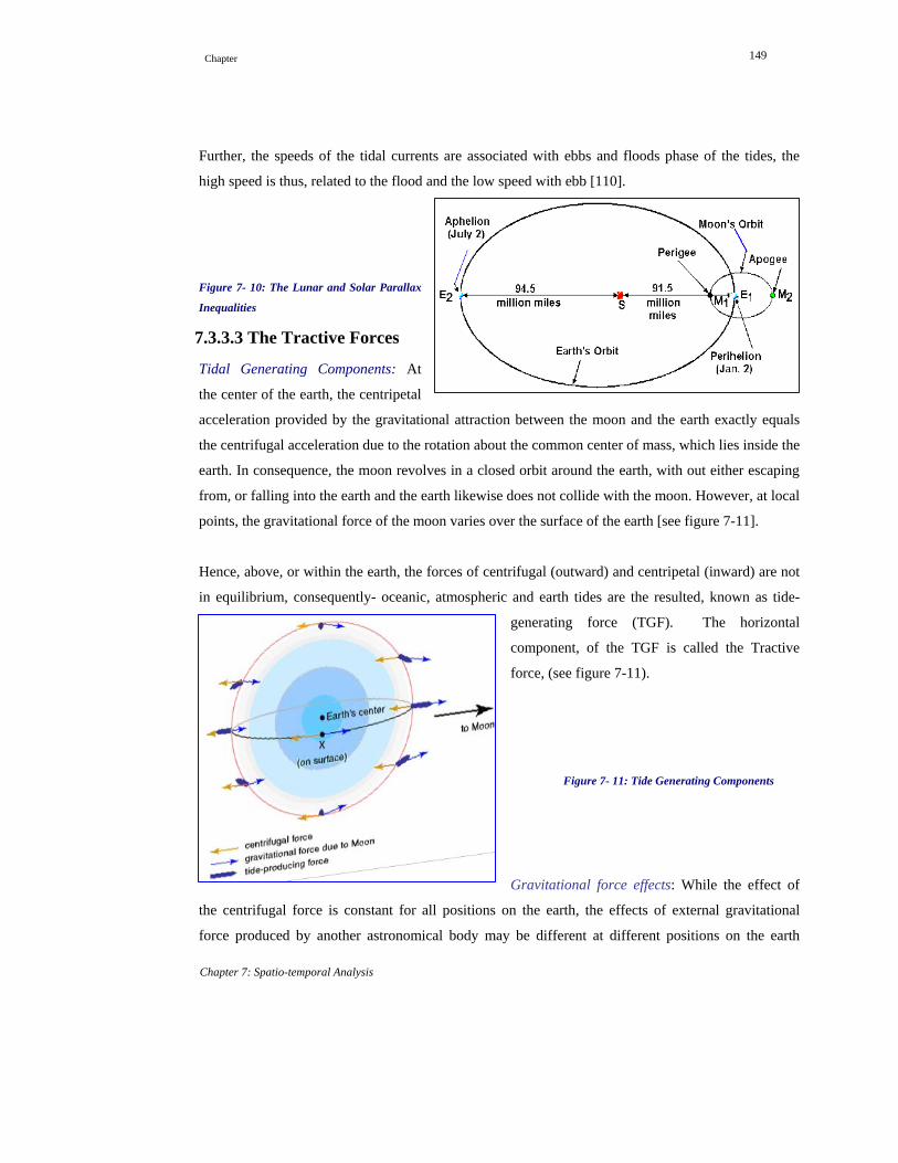
Chapter 149


Further, the speeds of the tidal currents are associated with ebbs and floods phase of the tides, the

high speed is thus, related to the flood and the low speed with ebb [110].

Figure 7- 10: The Lunar and Solar Parallax

Inequalities

7.3.3.3 The Tractive Forces

Tidal Generating Components: At

the center of the earth, the centripetal

acceleration provided by the gravitational attraction between the moon and the earth exactly equals

the centrifugal acceleration due to the rotation about the common center of mass, which lies inside the

earth. In consequence, the moon revolves in a closed orbit around the earth, with out either escaping

from, or falling into the earth and the earth likewise does not collide with the moon. However, at local

points, the gravitational force of the moon varies over the surface of the earth [see figure 7-11].

Hence, above, or within the earth, the forces of centrifugal (outward) and centripetal (inward) are not

in equilibrium, consequently- oceanic, atmospheric and earth tides are the resulted, known as tide-

generating force (TGF). The horizontal

component, of the TGF is called the Tractive

force, (see figure 7-11).

Figure 7- 11: Tide Generating Components

Gravitational force effects: While the effect of

the centrifugal force is constant for all positions on the earth, the effects of external gravitational

force produced by another astronomical body may be different at different positions on the earth

Chapter 150


because the magnitude of the gravitational force varies with distance of the attracting body [105]. The

relative gravitational force exerted at various positions is indicated in figure 7-12.

Net Tide-Raising Forces: Referring to figure 7-12, the center-of-mass of the earth and moon remain

in equilibrium at constant distances from the barycentre. The centrifugal force acting upon the center

of the earth (Point C) must be equal and opposite to the gravitational forces exerted by the moon on

the center of the earth [104]. At point A (see figure 7-12), the force produced by the gravitational pull

of the moon is considerably larger than the gravitational force at C due to the moon.

The net tide producing force at A obtained by taking the difference between the gravitational force

and the centrifugal forces is in favor of the gravitational component outward towards the moon. The

tide raising force at point A is indicated by double arrow (see figure 7-12), extending vertical from

the surface of the earth towards the direction of the moon.

At point B: Since gravitational force is less at B than at C, it follows that, the centrifugal force

exerted at B is greater than the gravitational force exerted by the moon at point B. The resultant tide

producing force at this point is, therefore, directed away from the earth center and opposite to the

position of the moon.

The tide produced in this location halfway around the earth from the sub lunar point, coincidentally

with the direct tide, is known as the opposite tide.

Figure 7- 12: The

Combination of Force of

Lunar Origin Producing

Tides

The tide raising force

of the moon is,

entirely insufficient

to” LIFT” the waters

physically against the

far greater pull of

Chapter 151


earth gravity. Instead, the tides are produced by the component of the tide- raising force of the moon,

which acts to draw the waters of the earth horizontally over its surface towards the sub lunar and

antipodal points [104].

Hence, at any point of the earth surface the tidal force produced by the moon’s gravitational attraction

may be resolved into two components: -

(a)Vertical or perpendicular to the earth surface and (b) horizontal or tangent to the earth surface, the

second component known as Tractive (drawing) component of force is the actual mechanism for

producing the tides.

Figure 7-13: The Moon's Declination Effect on

tides (Semidiurnal, Mixed, and Diurnal Tides)

These horizontal gravitational components, (TGF) cause the result of having two highs and two lows

per lunar day. Thus, there exist an active tendency for water to be drawn from other points on the

earth surface towards the sub lunar (point A) and antipodal (point B) (see figure 7-13) and to heaped

in the two points in two tidal bulges, due to the effects and strength of gravitational and centrifugal

forces.

7.3.4 The possible Types of Tides

A short description of the types of tides related to the explained theoretical processes is given below.

The positional declination effects (see figure 7-13) of the moon with respect of the equator on the

types of tides and the graphical visualization of the types of the tides that occur at different phases are

also explained (see figure 7-14).

Diurnal tides: Tides vary from day to day and from place to place. The geometric relationship of the

moon and sun to locations on earth surface and other influencing factors cause the creation of three

different types of tides [106].

As they (earth and moon) orbit, their positions shift, causing slight variation in gravitational effects

and initiates tides occurrence. In Figure 7-13, for example, the point C is seen to lie beneath a portion

of the tidal force envelopes. One half day later, as this point rotates to point C’ it is seen to lie above

Chapter 152


the tide force envelop. At this location, therefore, the tidal forces produce only one high water and

one low water each day, [106]. These tides are called diurnal tides, (see figures 7-13 and 7-14 C).

Semidiurnal Tide: When the two highs and the two lows are about the same height, the pattern is

called a semi-daily or semidiurnal tide. Consequently, successive highs and successive low are also

nearly equally spaced in time and occur twice daily. (See figure 7-13 and figure 7-14, A). So, tidal

data range related to the equatorial part of the earth falls to this category.

Mixed tide: However when the changing angular distance of the moon is above or below the equator,

the tidal forces envelop

produced by the moon is

canted or changed, and the

difference between the

heights of two daily tides of

the same phase began to

occur. This situation gives

rise to a twice-daily tide

displaying unequal heights

in successive highs or low

tides with strong diurnal

inequality (see figures 7-13

and 7-14, B).

Figure 7- 14: Principal Types of Tides

http://www.physicalgeography.net/physgeoglos/d.html#anchor586092

Chapter 7 153


Ch t II apter 7: Spatio-Temporal Analysis Par

7.4: Tidal Current’s Velocity and Direction Analysis

7.4.1 Nature of the tidal data

Measurement data related to the coastal

current (speed and direction), collected in

five different locations, have been

employed to interpret and understand the

current situation in the Guayaquil estuary.

These data are referenced by longitude,

latitude, depth or elevation (LLE), and a

specific time (hr) in a particular day.

Figure 7- 15: Measurement Stations

Thus, the five stations’ data reflect each

day’s (for 5 days) measurement (see table

7-1). No two or more stations were

measured in the same date. Furthermore, one station (3) is characterized by tide type (ebb and flood)

related to the quadrature positional phase of the moon (where moon and sun are perpendicular to each

other and the gravitational forces are counteracted to produced a lower bulge of tide on the earth,

known as neap tide).

On the other hand, the remaining stations are related to the positional phase of the moon (syzygy)

where both the moon and sun are aligned, and the cumulative forces create higher bulge of tide on the

earth known as the spring tide.

Table 7-1: Physical Data Summary

Chapter 7 154


With such kind of data, the water current’s velocity and direction analysis is supposed to be restricted

to date/time, elevation on a specific day uniquely. Example, a question such as what was the velocity

of the current at 7:00 AM at a specific LLE and STATION can be retrieved and its spatio-temporal

relationship visualized.

On the other-hand, the reverse of

the question “what was the

current velocity in all STATIONS

at a particular LLE, and

DATE/TIME cannot be retrieved

due to the fact that no two or

more stations were measured in

the same day. Nevertheless, such

limitations can be avoided by data

acquired simultaneously at

multiple stations.

Figure 7- 16: Structural Relationship of

the Physical and Spatio-Temporal Data

7.4.2 Analysis Processes and Results

Based on the conceptual relationship of the data models (see figure 7-16), the spatio-temporal

situation of the current velocity and direction analysis has been realized.

Conditions that reveal the dynamicity of the current (current velocity cm/sec and current direction

deg/mag) at different depths on particular time in a station have been executed applying the

contrasted mean and measured value distribution of velocity (cm/sec) and current direction (deg/mag)

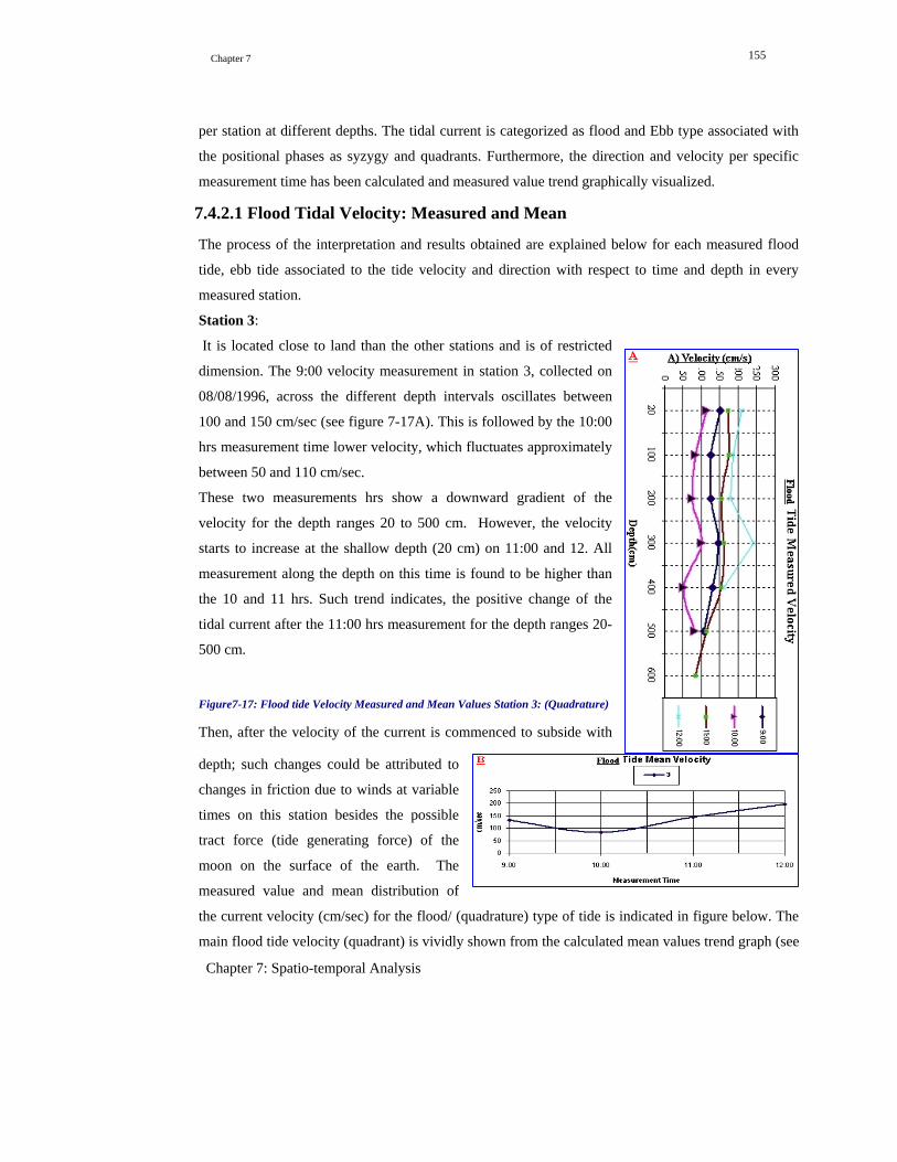
Chapter 7 155


per station at different depths. The tidal current is categorized as flood and Ebb type associated with

the positional phases as syzygy and quadrants. Furthermore, the direction and velocity per specific

measurement time has been calculated and measured value trend graphically visualized.

7.4.2.1 Flood Tidal Velocity: Measured and Mean

The process of the interpretation and results obtained are explained below for each measured flood

tide, ebb tide associated to the tide velocity and direction with respect to time and depth in every

measured station.

Station 3:

It is located close to land than the other stations and is of restricted

dimension. The 9:00 velocity measurement in station 3, collected on

08/08/1996, across the different depth intervals oscillates between

100 and 150 cm/sec (see figure 7-17A). This is followed by the 10:00

hrs measurement time lower velocity, which fluctuates approximately

between 50 and 110 cm/sec.

These two measurements hrs show a downward gradient of the

velocity for the depth ranges 20 to 500 cm. However, the velocity

starts to increase at the shallow depth (20 cm) on 11:00 and 12. All

measurement along the depth on this time is found to be higher than

the 10 and 11 hrs. Such trend indicates, the positive change of the

tidal current after the 11:00 hrs measurement for the depth ranges 20-

500 cm.

Figure7-17: Flood tide Velocity Measured and Mean Values Station 3: (Quadrature)

Then, after the velocity of the current is commenced to subside with

depth; such changes could be attributed to

changes in friction due to winds at variable

times on this station besides the possible

tract force (tide generating force) of the

moon on the surface of the earth. The

measured value and mean distribution of

the current velocity (cm/sec) for the flood/ (quadrature) type of tide is indicated in figure below. The

main flood tide velocity (quadrant) is vividly shown from the calculated mean values trend graph (see

Chapter 7 156


figure 7-17B). It is revealed that flood tide velocity between 9:00 and 10:00 displays a higher to lower

145 cm/sec and 10:00 12:00 an ascending trend of 85 cm/sec respectively.

Station 10:

The station is situated close to the southern edge of the estuary (see figure 7-18) is relatively wider

channel compared to stations 3 and 7.

With regard to the measured velocity, the lowest tidal velocity (associated to syzygy), collected on

08/ 14/ 1996) occurs close to the surface water across all the depths in the 13:00, followed by the

14:00 measurements time.

Therefore, no significant difference exists between shallow and

relatively deeper water medium between the 13:00 and 14:00

measurement hours.

The min and max range for both measurement times is found to be 25-

50 cm/sec and 55-85 cm/sec respectively.

However, during the 15:00, there relatively occurs a sharp increase of

water current velocity from 20 to 400 cm and subsequently it remains

high speed along the depth range 400 to 1000 cm; but the trend of the

velocity descends with depth until 1400 cm.

Figure 7-18: Flood tide (syzygy): Measured and

Mean Values Station 10

Chapter 7 157


This feature is established both by the measured flood tide of time vs. depth and mean value

distribution (see figure 7-18). Three conditions are established: -

Low tidal current water between 13:00 and 14: 00 along all the measurement points in this station,

which suggest a calm environment; Between 15 and 16hrs the situation changes and higher tidal

current is prevailed, mainly between 150 and 1050 cm; The general mean velocity discerns an

increasing trend of the tidal to be between 13 and 16 hrs.

Station 7:

Topographically, station 7 is described to be of a narrow morphology (see figure 7-19). The

measured data, near surface, on 20/08/1996, (associated with syzygy)

water current shows a lower velocity fluctuation between 75, 25 cm/sec,

100, and 75 cm/sec at 11:00 and 12:00 respectively. However, the

velocity descends around the 1050 cm to a rate of 50 to 25 cm/sec. The

change of the velocity rate at (A) surface is related to frictional force, (B)

at relatively higher depth to low friction water column and (C) at very

low of velocity corresponding to higher depth due to changes of the

morphology.

The mean velocity associated with the flood tide discloses increase of the

velocity 11:00-13:00 and descends gradually towards 15:00. The

interpretation result suggests that the dimension of the channel might be

wider at depth than at the surface and current spread across the channel at

a lower magnitude as observed with the depth range of 900- 1200 cm.

Figure 7-19: Flood tide (syzygy): Measured and Mean Values Station 7

Chapter 7 158


Station 13: This station is located in the western part of the estuary channel and is

also close to the open ocean.

Referring to figure 7-20a, measurement data of 08/15/1996, (associated

to syzygy) of the 13:00 measurement shows low velocity values near

surface water (unlike to the 14:00, 15:00, 16:00 and 17:00 hrs, across all

the depths (see figure7-20A) which are characterized by higher

velocity).

This phenomenon with respect to time of measurements is well

established by the mean value graphic display (see figure7-20B), related

to the flood measured velocity in station 13.


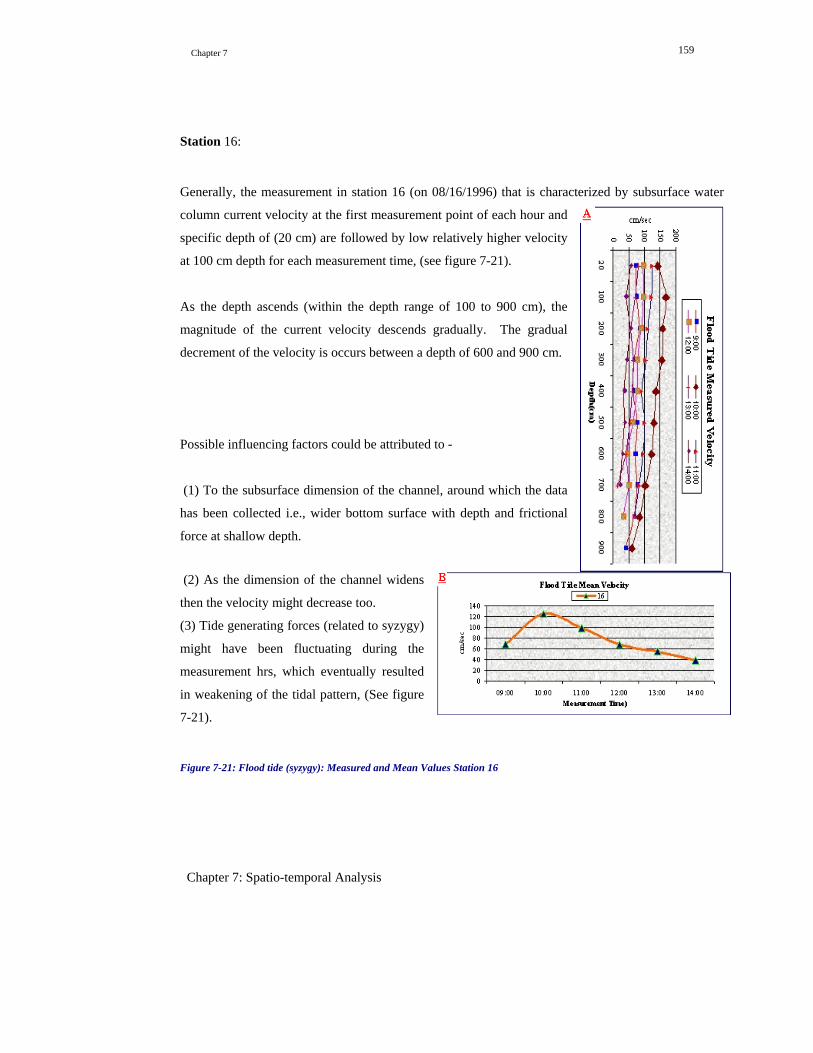
Chapter 7 159


Station 16: Generally, the measurement in station 16 (on 08/16/1996) that is characterized by subsurface water

column current velocity at the first measurement point of each hour and

specific depth of (20 cm) are followed by low relatively higher velocity

at 100 cm depth for each measurement time, (see figure 7-21).

As the depth ascends (within the depth range of 100 to 900 cm), the

magnitude of the current velocity descends gradually. The gradual

decrement of the velocity is occurs between a depth of 600 and 900 cm.

Possible influencing factors could be attributed to -

(1) To the subsurface dimension of the channel, around which the data

has been collected i.e., wider bottom surface with depth and frictional

force at shallow depth.

(2) As the dimension of the channel widens

then the velocity might decrease too.

(3) Tide generating forces (related to syzygy)

might have been fluctuating during the

measurement hrs, which eventually resulted

in weakening of the tidal pattern, (See figure

7-21).


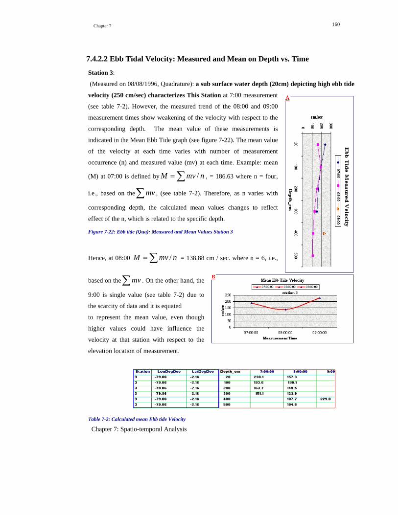
Chapter 7 160


7.4.2.2 Ebb Tidal Velocity: Measured and Mean on Depth vs. Time

Station 3:

(Measured on 08/08/1996, Quadrature): a sub surface water depth (20cm) depicting high ebb tide

velocity (250 cm/sec) characterizes This Station at 7:00 measurement

(see table 7-2). However, the measured trend of the 08:00 and 09:00

measurement times show weakening of the velocity with respect to the

corresponding depth. The mean value of these measurements is

indicated in the Mean Ebb Tide graph (see figure 7-22). The mean value

of the velocity at each time varies with number of measurement

occurrence (n) and measured value (mv) at each time. Example: mean

(M) at 07:00 is defined by ∑= nmvM / , = 186.63 where n = four,

i.e., based on the , (see table 7-2). Therefore, as n varies with

corresponding depth, the calculated mean values changes to reflect

effect of the n, which is related to the specific depth.

∑mv

Figure 7-22: Ebb tide (Qua): Measured and Mean Values Station 3

Hence, at 08:00 = 138.88 cm / sec. where n = 6, i.e.,

based on the∑ . On the other hand, the

9:00 is single value (see table 7-2) due to

the scarcity of data and it is equated

∑= nmvM /

mv

to represent the mean value, even though

higher values could have influence the

velocity at that station with respect to the

elevation location of measurement.

Table 7-2: Calculated mean Ebb tide Velocity

Chapter 7 161


Station 10:

The ebb tidal velocity on station 10, collected on 08/14/96, associated

to sygyzy shows highest velocity at 10:00, followed by low value of

the measurement times of 11:00 and 12:00 (see figure 7-23).

The number of measurement occurrence (n) for station 10, depth range

20 to 1400 cm are defined as follows; time (t) 10:00 = 15, time (t)

11:00 = 9, time (t) 12:00 = 12 respectively.

Thus, the mean value of the velocity varies with the n, which is

established by . ∑= nmvM /

The general trend conforms to a reciprocal relationship of velocity vs.

depth as shown by the fluctuating and diminution of the current

velocity (see figure 7-23).

Figure 7-23: Ebb tide (syzygy): Measured and Mean Values Station 10

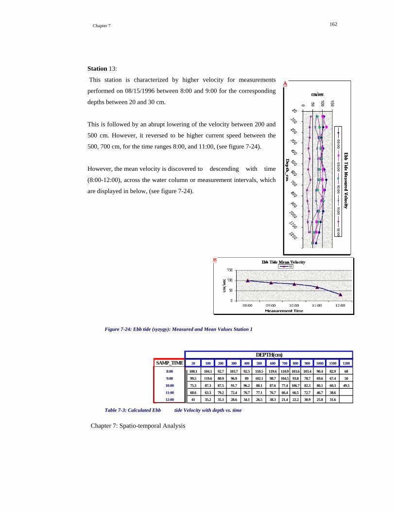
Chapter 7 162


SAMP_TIME 20 100 200 300 400 500 600 700 800 900 1000 1100 1200

8:00 108.1 104.1 92.7 103.7 92.5 110.5 119.6 110.9 103.6 103.4 90.4 82.9 68

9:00 99.5 119.6 80.9 96.9 89 102.1 98.7 104.5 93.8 78.7 69.6 67.4 50

10:00 75.3 87.3 87.5 91.7 96.2 88.1 87.6 77.4 106.7 82.3 80.1 60.3 49.5

11:00 68.6 63.3 79.2 72.4 76.7 77.1 76.7 66.4 66.5 72.7 46.7 38.6

12:00 41 35.2 35.3 28.6 34.1 26.5 38.3 21.4 22.2 30.9 25.8 31.6

DEPTH(cm

Station 13:

This station is characterized by higher velocity for measurements

performed on 08/15/1996 between 8:00 and 9:00 for the corresponding

depths between 20 and 30 cm.

This is followed by an abrupt lowering of the velocity between 200 and

500 cm. However, it reversed to be higher current speed between the

500, 700 cm, for the time ranges 8:00, and 11:00, (see figure 7-24).

However, the mean velocity is discovered to descending with time

(8:00-12:00), across the water column or measurement intervals, which

are displayed in below, (see figure 7-24).


)

Table 7-3: Calculated Ebb tide Velocity with depth vs. time

Chapter 7 163


Station 7: Measurements performed on 20/08/96, in this station discerns certain oscillating pattern. For

instance, the tide velocity on the depth of 20 cm at 11:00 is a little greater than 50 cm per second; at

same depth but different measurement time (11:00 and 13:00), the

velocity range is augmented dramatically to 80 and 120 cm/sec

respectively.

This indicates velocity increase between 11:00 and 12:00 at and around

the depth of 20 cm, for the 11:00 measurements.

Furthermore, as the depth increases from 20 to 300 cm, (see figure 7-

25A), the corresponding velocity decreases.

The measurement documentation associated to this particular data

indicates to the ebb tide type related to the syzygy positional phase of

the moon.

The mean value of the measured velocity based on the occurrences of

the depths shows an increase of the ebb velocity from the morning

towards the after noon with peak value being between 12:00 and 13:00

hrs (see figure 7-25B).

Figure 7-25: Ebb tide (syzygy): Measured and Mean

Values Station 7

Chapter 7 164


Station16: Geographically, station 16 is closer to the coastal land than to the main gulf of the estuary.

All the measurements times, in this station, related to the date of

08/16/96, show relatively lower current velocity at the 20 cm depths,

(see figure 7-26).

This magnitude descends gently as the depth is elevated from 100 to 900

cm, for all measurements periods except 10:00, which shows specific

peak at 100 cm.

This phase from low to high tends to subside gradually to indicate the

changes in the ebb tide generating forces at different levels of the water

column. Despite of the certain irregularity of the tidal current velocity

the trend significantly discerns the lowering of the velocity with depth.

Also, the over all mean velocity discerns a highest phase to coincide

around the 100 cm and the trend the mean velocity cm/sec, found to

gradually fall down with the increment of the depth and measurement

time from 11:00 towards 14:00 hrs(see figure 7-26 A+B)


Chapter 7 165


7.4.2.3 Ebb Tidal Velocity Direction: Measured and Mean with Depth vs. Time

Station 3:

Measurement related to the Ebb Tidal Velocity Direction is charactrized by the depth level and the

corresponding deviation of the velocity direction in magnetic degree.

According to the measurement data, the graphical visualization of the

ebb tide velocity direction shows high, low, high and low directional

values.

This means that the direction fluctuates with increase of depth from

S.West to S.East. For instance, the 200-measured degree (at 7:00)

indicates the S.West direction and the 150 at a depth of 500 cm is

S.East; see figure 7-27B and 7-27A respectively.

The interpretation is based on the geographical reading of the measured

degree with respect to the Georeferenced map which contains the all the

measurement sites.

This can be explained using the style of geography reading (0 degree =

N, 90 degree =E, 180 degree = S and 270degree = W).

The mean value directional changes, as

indicated by the measurement time (7:00 to

9:00) where the current velocity shifts its

direction relatively from southwest towards

southeast.

Figure 7-27: Ebb tide Direction (Quadrature): Measured and Mean Values Station 3

Probably, this could be attributed to the effects of the variation of changes in sub water topography

or change on the intensity of the current velocity due to TGF.

Chapter 7 166


Station 7: The station is located within a narrow channel of the statuary and is

closer to coastal land than the stations 10, 13.

Since the dimension of the channel where this station is located is of

restricted dimension, the possibility of the deviation of the current

velocity is subjected to channel dimension controlled.

The measurements of the current direction between 12:00 and 15:00

(20/08/1996) show a pattern of little variation at all measured depths

(see figure 7-28A).

The trend from southwest to southeast is associated with the slight

perturbation of the direction observed on the 12:00 measurement time

and along with depth increment. In other wards, the trend fluctuation is

restricted within the 150 to 200 degree.

The calculated mean tidal direction (see

figure 7-28B).ranges shows between170 and

180 degree between the measurement times

of 12:00 and 15:00.

Figure 7-28: Ebb tide Direction (Quadrature): Measured & Mean Value Station 7

The results suggest a deviation of the current from South East to South, which corresponds to the

mean degree direction of 170 to 180. It is unveiled that this current velocity direction continues to

persist between measurement times of 14:00 and 15:00. Further more the trend seems to extend

beyond the 14:00 with a north-south direction.

Chapter 7 167


Station 10:

This station is close to the mouth of the sea and is relatively a wider channel, for instance, compared

to station 3 and station 7.

The tidal current velocity directional measurement depth between 20 and 1000 cm ranges 105 to 153

degrees and it falls from East to S.East flowing direction

category. However, there is rather a phase of the direction where

all the different depths to indicate current velocity direction to

follow a southeast direction, especially between the depth

intervals 200 and 600 cm, (see figure 7-29A).

On the other hand, around 1200 cm, the measurements of the

11:00 shows a current velocity direction towards the east whereas

at the same (x, y, z) but different t, 12:00 the velocity direction

tends to deviate towards the south.

This result is interpreted to be due the change of tide generating

forces in the same x, y, and z but at different times, i.e., 11:00

and 12:00.

This pattern is well visualized by the mean values along the

measurement times (see figure 7-29B). The mean value Ebb tide

current velocity direction also shows a persistence of the

direction between the measurement times between 10:00 and

11:00 along the 150 degree (South East).

Figure 7-29: Ebb tide Direction (Quadrature): Measured and Mean Values Station 10

Chapter 7 168


Station 13: This station is characterized by a certain regularity of velocity direction around the 200-250 degree

(S.West) along all the measured depths; with the exception of 12:00 (see figure 7-30A), which

indicates certain perturbation on the depth ranging 400-900. The relatively similar direction is

observed along all the depths measured on the 8:00, 9:00 and 10:00 measurement time.

However, the 12:00 hrs measurements mean value shows a shift of a

westward direction, and this high value is indicated in the measured

velocity direction to occur around the depth of 800 cm (see figure 7-30).

The later results indicate initiation of change in the tide generating force

phase, which is completely different from the previous measurements.

Base on the results of the current direction, it seems possible to indicate

anticipation of tidal changes.

Figure 7-30: Ebb tide Direction (syzygy): Measured & Mean Values Station 13

Chapter 7 169


Station 16: Measurements on this site do not show significant variation in velocity direction. The range of

direction recorded is shown to be within 170 and 200 degree.

The first 150 cm depth along all the measurements points (x, y, z on different times) described by

SE-SW trend; However, at a depth of 250 cm, deviation of the velocity direction coincides to be

South Westerly (200 degree) on all the measurements times (9:00 to

13:00).

With the exception of measurement time 13:00, which shows slight

directional fluctuations (see figure 7-32 A+B), the others display a

regular SW velocity direction along all the measurement depths on all

the different times.

As the depth decreases (900 cm), the velocity direction changes

towards the South, which is discerned by the converging lines (see

figure 7-31A) and the falling trend line, i.e. mean velocity direction

distribution, (see figure 7-31B).

Figure 7-31: Ebb tide Direction (Quadrature): Measured & Mean Values Station 16

Chapter 7 170


7.4.2.4 Current’s Velocity and Direction (Ebb tide)

in all stations

I. Velocity

Velocity: Velocity with respect to time and depth

0 to 9:00 - 8:00 Lower phase of the current velocity

Around 10:00 – Highest phase of the current velocity

11:00 to 14:00 – Descending phase of the current velocity

The velocity in station 10 is shown to be with highest mean,

mainly with the depth range 150-900 (cm) and descends to

lowest phase around the depth of 1300 -+ 50 cm.

The same trend has been unveiled on the other stations (7, 16,

and 13) but with less mean value than station, 10(see figure 7-

32)

Figure 7-32: Ebb tide Velocity: Measured and Mean

Values in Stations (7, 10, 13, and 16)

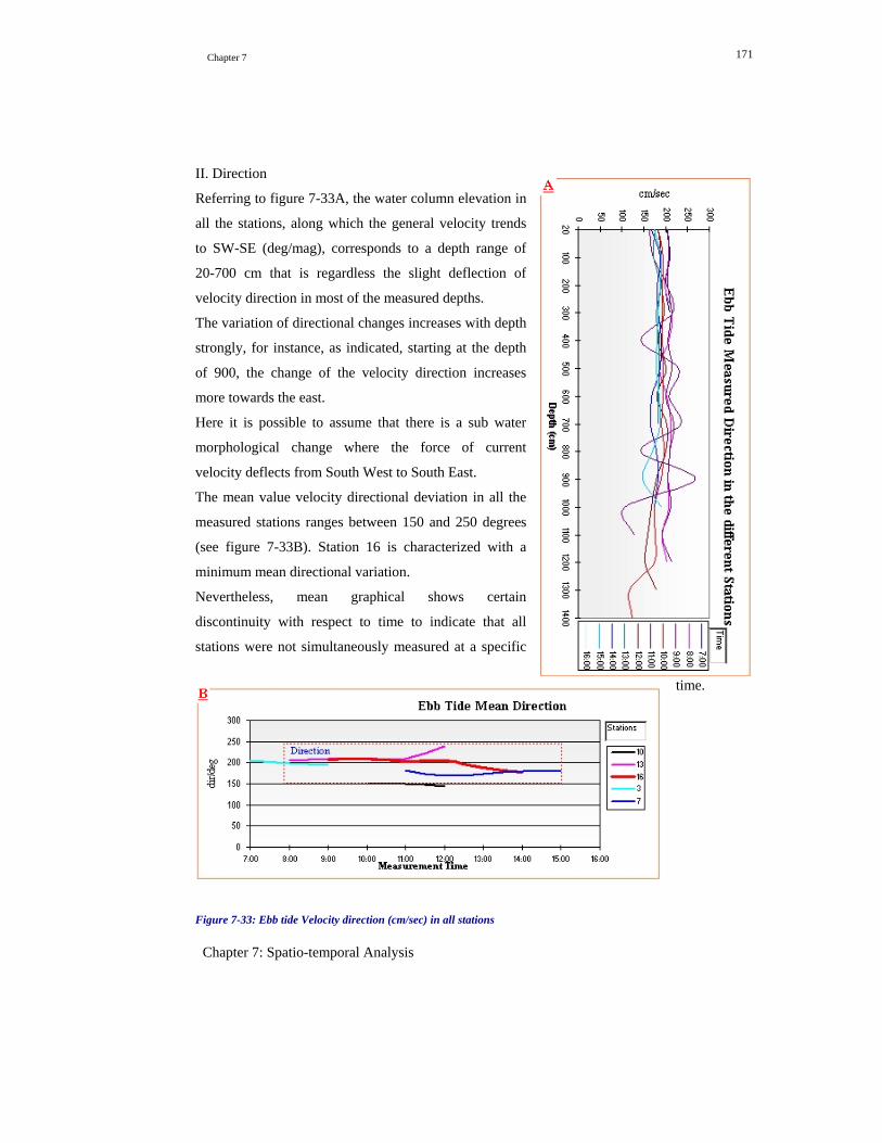
Chapter 7 171


II. Direction

Referring to figure 7-33A, the water column elevation in

all the stations, along which the general velocity trends

to SW-SE (deg/mag), corresponds to a depth range of

20-700 cm that is regardless the slight deflection of

velocity direction in most of the measured depths.

The variation of directional changes increases with depth

strongly, for instance, as indicated, starting at the depth

of 900, the change of the velocity direction increases

more towards the east.

Here it is possible to assume that there is a sub water

morphological change where the force of current

velocity deflects from South West to South East.

The mean value velocity directional deviation in all the

measured stations ranges between 150 and 250 degrees

(see figure 7-33B). Station 16 is characterized with a

minimum mean directional variation.

Nevertheless, mean graphical shows certain

discontinuity with respect to time to indicate that all

stations were not simultaneously measured at a specific

time.

Figure 7-33: Ebb tide Velocity direction (cm/sec) in all stations

Chapter 7 172


7.4.3. Flood Tide Velocity

A 3D line graph has been used to visualize the flood tide velocity with respect to time and depth data

(see table 7-4) in the different measurement stations, which is described as follows. As depth

increases, the flood tide velocity (measured velocity cm/sec) decreases to the lowest magnitude

between depths ranges of 800-1400 cm and respective corresponding measurement times (see figure

7-35).

Table 7-4: Calculated Flood tide Velocity with time vs. depth

Chapter 7 173


Figure 7-34: Flood tide Velocity direction (cm/sec) in all stations

For instance, the 13:00 measurement results show the lowest occurrence of the velocity in the

specified time of the day along all the measured depths (20-1400 cm).

On the other hand, the 16:00 results reflect the tidal velocity ranges 63.2-182 cm/sec with respect to

depth 1400 and 200 cm (see table 7-4). Some possible causes to the depletion or wedging out of the

current velocity with depth can be attributed to a dimensional change of the channel with depth,

which disperses the speed on the extended space and fluctuation of the tide generating tract forces.

7.4.4. Geo-referenced Spatio-temporal Interpretation

Velocity Direction at Specific Time (ebb): One of the important applications of GIS is its capability

to process and perform spatial analysis on the data with respect to geo-referenced sites. Also as the

application is extended to incorporate data associated with temporal parameters and visualize the

information with view to the time associated during the genesis of the data in the environment where

it was

acquired

for

example at

10h, 11h

and 12h,

that is in

different

stations

(see figure

7-35). The

indicated

Figure 7-35: Georeferenced Spatio-Temporal Visualization of Velocity Directions (ebb tide)

Chapter 7 174


Measurement times were selected because they contain data that can be represented and relevantly

interpreted in the respective stations (see figure 7-35 and 7-36) without discontinuity

With this, regard the deviation of the current velocity direction, based on the geodatabase attribute

values have been sptaio-temporally processed and revealed the following results (see figure 7-36)

Figure 7-36: Georeferenced Spatio-Temporal Visualization of Velocity Directions (Flood tide)

Tidal Velocity at Specific Time flood: Combining the thematical views of velocity direction

(mag/deg) and velocity (cm/sec) information enables us to asses the nature of the dynamicity and

fluctuations of the current in different sites of measurements.

The resymbolised dimension indicates the magnitude of the current velocity in that particular station

with respect to the time of measurement. According to the results of the analysis indicated (see figure

7-37), the highest range of the velocity associated to the situation of the syzygy occurs in station 7

and lowest in station 10.

Such occurrence is attributed to the strength of the tidal force components, which is stronger due to

the alignment of the celestial bodies (syzygy), would eventually enhances the gravitational force on a

Chapter 7 175


specific site on earth surface. Under such systems interaction, the tidal currents are prone to

influences which could be detected during relevant measurements and the processed data can be

visualized spatio-temporally as illustrated in figure 7-37, for the flood tide related current velocity

(cm/sec) at a specific time

Figure 7-37: Spatio-Temporal Visualization of Mean Velocity and Direction at a specific time

Otherwise, station 10 is uncovered to have not the characteristics of station 7. This is attributed due to

morphological difference (relatively wider) and proximity of the geographical proximity towards the

open sea. The velocity of the current might diminish with increment of the width and the tract forces

could have been at their lowest phase during the measurement. Nevertheless, one can see that

whenever a high-density measurement data are available, GIS is a tool that can be applied to analyze

the problem spatio-temporally and visualize the results thematically.

Chapter 7 176


7.5. Results and Conclusions a) The process of spatio-temporal analysis associated geographic features and tagged temporal

parameters are complex. This fact is supported by the practical dependence of location-based

information on time when many attribute data are collected in a single geo-referenced point at

different times. The problem related to such spatial information layers representation i.e., as function

of time has been resolved by formulating the layers of the associated features and temporal

parameters as follows.

Layer (n) = F (Tn) on X, Y, (+ - (Z), m:

Where n in Layer (n) is number of layers, n in (Tn) is number of occurrence time, X, Y and Z are the

coordinates and the m is possible measured value. The variation of m as a function of Tn has been

retrieved based on - Ln+1 = f (Tn+1) on X, Y, (+ - (Z), m)

b) Spatio-temporal information is indexed with time. It becomes easier said than done to represent it

thematically especially when multiple measured attributes (m) are associated and referenced to 2D

features. Such difficulties have been sorted out by aggregating methodology, which encompass

converting (of objects) mapping relationship of 1: M to 1:1. The following principle illustrates the

process: Analyzing features (•ro changes to •r1 and •r1 to •r2) function of time, f (t), at x, y, (+ - (z);

1) • S1 > •to > •ro > •A

2) Layer1 (S1) = f (t1): r1 ↓

3) Layer1 (S1) = f (t2): r2 ↓

… Layer (Sn) = f (tn+1): r n+1

Thus, the layer corresponding to A (aggregate) is processed as: -

3) Layer (Sn) = f (tn): f (rn+1)

c) A certain relationship between the current velocity and the depth environment along all the

measurement stations shows a situation of a higher depth corresponds to diminishing of the current

velocity. Likewise, the velocity of the current associated with the flood tide wedges out with depth.

These results suggest the possible morphological change of the estuary channel at depth or weakening

Chapter 7 177


of the current due to friction at top water surface and possible fluctuation of the tide generating force

(TF) at the sites of measurements.

d) The result at measurement time of 10:00, along all the measured depth related ebb tidal current

velocity shows higher tidal activity phase contrary to the phase of the velocity in the time interval

between 13:00 and 14:00 (see figure 7-33).

Furthermore, the 12:00 measurement time, related to azimuth/ebb tide velocity directional fluctuation,

on the eastern and western channels shows an opposing trend. The S to SW and S to SE describe this

direction and it rather tends to follow the trend of the major channels (see figure 7-37).

e) Referring to the figure 7-34, the ebb tide velocity associated to the positional phase of the moon

(syzygy) shows a Time vs. Depth related fluctuations. With this regard, the measurement time

ranging of 8:00 –8:30 indicates the descending of higher velocity to lower velocity and the 8:30 to

10:30 discloses the peak velocity which coincides to the 10:00+-00:20; and 10:20 to 15:00 displays

the diminution of the velocity from lower to lowest phase. The situation could be attributed to the

opposing frictional force at the surface, a calm environment of water column above the highest depth

and morphological change of t channel at depth.

e) The temporal analysis results are derived from very few and widely dispersed measurement

stations and limited respective depths. The methodology of interpretation can be implemented to

unveil the relationship of tidal current speed and direction within an estuary in a better way by

increasing the measurement density and incorporating more data types into the developed object

relational geodatabase. Nevertheless, results obtained from such process can be exploited in grasping

natural dynamic process and gauge human induced effects through time in the area of interest.

Chapter 8: 178

Chapter 8 : Aspatial Analysis

8.1 Introduction

The two preceding chapters have been focused on the spatial and spatio-temporal analysis

processes. Space and/or time were incorporated as main components in spatial and spatio-

temporal query. The theme of this chapter deals with aspatial analysis perception.

Aspatial is a term that used to describe non-spatial data associated to geographic objects [40].

Compositionally, aspatial data are heterogeneous in nature and are more complex when a

multidisciplinary teams function together in an integrated Coastal/Marine environment GIS

projects. They are valuable information assets and the potentiality of the value is appreciated

when processed meticulously not only taking into consideration the spatial context

(Georeferenced) but also analyze with respect to aspatial perspectives.

8.2 Aspatial Analysis Query (AAQ)

SQL Query Design: Query design is one of the most important components in the exploitation of

the geodatabase. SQL is an interactive and powerful non-procedural program language, close to

the human language if frequently used. The style of the aspatial query resembles that of spatial,

but it does not need any spatial operator but its efficient retrieval depends on the interlocking

migrating pointers.

8.2.1 Retrieval Efficiency

When a table is stored on disk, it is referred as a file with rows and column. During information

extraction, the disk access is typically slow. Constructing an index file that provides a direct

access to the data in the database file minimizes slowness of accessing and retrieving the needed

information [61]. Indexing reduce the time to find and process information within the

geodatabase. Figure 8-1A and figure 8-1B illustrates the possibility of data processing and

analysis using Linked tables information flow (figure 8-1A) (Location, Measurement Results, and

Field) and the corresponding SQL retrieving code is displayed (see figure 8-1B).

Figure 8-1 Tir-Table Information Extraction on a defined Relationship

Chapter 8: Aspatial Analysis

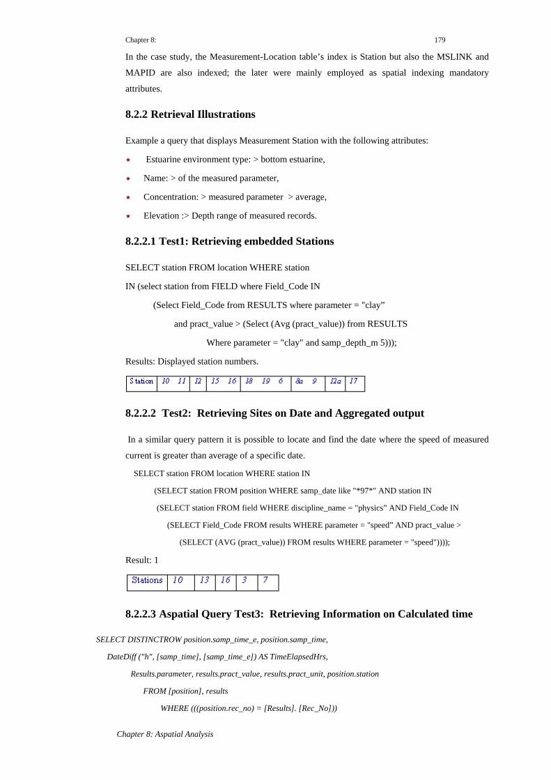
Chapter 8: 179

In the case study, the Measurement-Location table’s index is Station but also the MSLINK and

MAPID are also indexed; the later were mainly employed as spatial indexing mandatory

attributes.

8.2.2 Retrieval Illustrations

Example a query that displays Measurement Station with the following attributes:

Estuarine environment type: > bottom estuarine,

Name: > of the measured parameter,

Concentration: > measured parameter > average,

Elevation :> Depth range of measured records.

8.2.2.1 Test1: Retrieving embedded Stations

SELECT station FROM location WHERE station

IN (select station from FIELD where Field_Code IN

(Select Field_Code from RESULTS where parameter = "clay”

and pract_value > (Select (Avg (pract_value)) from RESULTS

Where parameter = "clay" and samp_depth_m 5)));

Results: Displayed station numbers.

8.2.2.2 Test2: Retrieving Sites on Date and Aggregated output

In a similar query pattern it is possible to locate and find the date where the speed of measured

current is greater than average of a specific date.

SELECT station FROM location WHERE station IN

(SELECT station FROM position WHERE samp_date like "*97*" AND station IN

(SELECT station FROM field WHERE discipline_name = "physics” AND Field_Code IN

(SELECT Field_Code FROM results WHERE parameter = "speed” AND pract_value >

(SELECT (AVG (pract_value)) FROM results WHERE parameter = "speed"))));

Result: 1

8.2.2.3 Aspatial Query Test3: Retrieving Information on Calculated time

SELECT DISTINCTROW position.samp_time_e, position.samp_time,

DateDiff ("h", [samp_time], [samp_time_e]) AS TimeElapsedHrs,

Results.parameter, results.pract_value, results.pract_unit, position.station

FROM [position], results

WHERE (((position.rec_no) = [Results]. [Rec_No]))


Chapter 8: 180

GROUP BY position.samp_time_e, position.samp_time, results.parameter,

Results.pract_value, results.pract_unit, position.station HAVING

(((Position.samp_time_e) Is Not Null) AND ((results.parameter)="mercury"));

Result: 2

Table 8- 1 Retrieved Results

8.3 Interfacing the GIS database

SQL query is powerful and flexible as far as it is applied to the purpose designed for. However, a

novice user may encounter problem in typing SQL codes and retrieve properly the information.

This is commonly encountered during practical works. A solution to this is to develop a user-

friendly interface to perform operations on the underlying GIS database by clicking interfacial

controls associated program codes. As a result of, many related actions on the underlain database

are executed; some of which are:

Process and retrieve information and design re-executable complex analytical query Communicate the underlying database tables graphically Display thematical results in a object-control based interface Locate the processed GIS database information on map-like form interface, indicate the

coordinates pertaining to the list values

Figure 8-2 Information flow Diagram


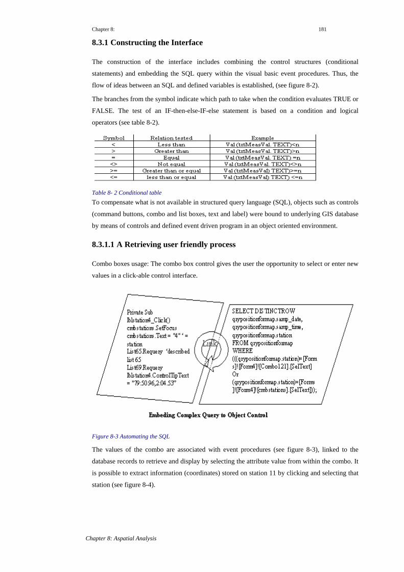
Chapter 8: 181

8.3.1 Constructing the Interface

The construction of the interface includes combining the control structures (conditional

statements) and embedding the SQL query within the visual basic event procedures. Thus, the

flow of ideas between an SQL and defined variables is established, (see figure 8-2).

The branches from the symbol indicate which path to take when the condition evaluates TRUE or

FALSE. The test of an IF-then-else-IF-else statement is based on a condition and logical

operators (see table 8-2).

Table 8- 2 Conditional table To compensate what is not available in structured query language (SQL), objects such as controls

(command buttons, combo and list boxes, text and label) were bound to underlying GIS database

by means of controls and defined event driven program in an object oriented environment.

8.3.1.1 A Retrieving user friendly process

Combo boxes usage: The combo box control gives the user the opportunity to select or enter new

values in a click-able control interface.

Figure 8-3 Automating the SQL

The values of the combo are associated with event procedures (see figure 8-3), linked to the

database records to retrieve and display by selecting the attribute value from within the combo. It

is possible to extract information (coordinates) stored on station 11 by clicking and selecting that

station (see figure 8-4).


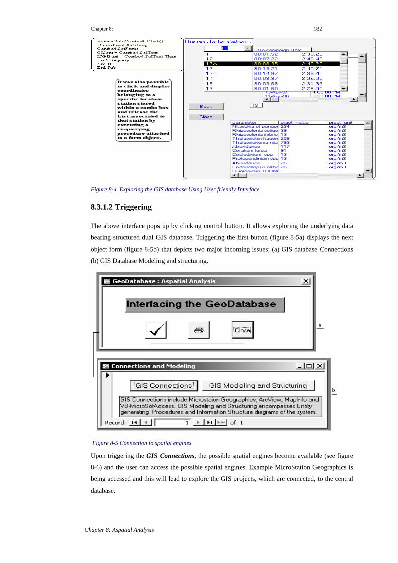
Chapter 8: 182

Figure 8-4 Exploring the GIS database Using User friendly Interface

8.3.1.2 Triggering

The above interface pops up by clicking control button. It allows exploring the underlying data

bearing structured dual GIS database. Triggering the first button (figure 8-5a) displays the next

object form (figure 8-5b) that depicts two major incoming issues; (a) GIS database Connections

(b) GIS Database Modeling and structuring.

Figure 8-5 Connection to spatial engines

Upon triggering the GIS Connections, the possible spatial engines become available (see figure

8-6) and the user can access the possible spatial engines. Example MicroStation Geographics is

being accessed and this will lead to explore the GIS projects, which are connected, to the central

database.


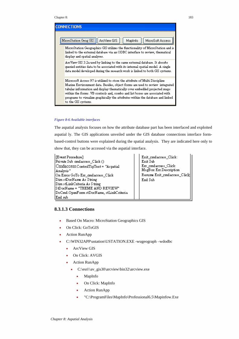
Chapter 8: 183


Figure 8-6 Available interfaces

The aspatial analysis focuses on how the attribute database part has been interfaced and exploited

aspatial ly. The GIS applications unveiled under the GIS database connections interface form-

based-control buttons were explained during the spatial analysis. They are indicated here only to

show that, they can be accessed via the aspatial interface.

8.3.1.3 Connections

Based On Macro: MicroStation Geographics GIS

On Click: GoToGIS

Action RunApp

C:\WIN32APP\ustation\USTATION.EXE -wugeograph –wdodbc

ArcView GIS

On Click: AVGIS

Action RunApp

C:\esri\\av_gis30\arcview\bin32\arcview.exe

MapInfo

On Click: MapInfo

Action RunApp

"C:\ProgramFiles\MapInfo\Professional6.5\Mapinfow.Exe

Chapter 8: 184

A program associated with a control, used to open ensuing objects is described below.

Three important issues are disclosed as a result of triggering the VB-Microsoft Access control

(see figure 8-6). Whenever the Theme Display tool is triggered (see figure 8-7), then figure 8-8 is

disclosed with all the data processing interface buttons.

Figure 8-7 A) Thematic displays B) Review Info (C) Environment

8.3.2 Theme Display:

The theme display is based on a combination of the VB6 binding controls code program and embedded SQL

beneath the interface. As a result of triggering the Theme Display tool, an aspatial information-analyzing

interface is disclosed with a number of possible tools, see figure 8-8.

Figure 8-8 Theme and Associated Information


Chapter 8: 185

The above interface enables to extract instantaneously multi discipline information both

graphically and in a tabular environment. Clicking an area represented by a box on the site where

measurement has taken place will first display the georeferencing parameters stored within the

structured database. Thus, one can understand the location coordinates that extracted from the

underlying geodatabase abruptly without connecting the spatial engine. Eventually, the event

procedure drives and display the station number corresponding to the georeferencing parameters

within the given text box. After few seconds, the embedded SQL query is processed behind the

scene and releases the temporal parameters of that station, and is filled in the first list with filed

names date and sampling time:

Furthermore, process of calculation takes place within the geodatabase reservoir by selecting

analyzed data and compares with certain constants and display graphically, distinguished by

different colors. On the given instance, the red color shows values of the clay greater than 6.5

percent (figure 8-8).

8.3.3 Retrieving Options

8.3.3.1 By Event: Optional slot STATION

NAME: cmbstations

Row Source:

Select Distinctrow Station_Loc.Station, Station_Loc.Lon, Station_Loc.Lat

From Station_Loc;

Private Sub Cmbstations_Click () 'cmbstations is name of the event,

Dim MyString As String ‘MyString is a variable of string data

Cmbstations. SetFocus ‘ set focus inserts the cursor on box

MyString = cmbstations. SelText ‘Assignment of value clicked in the combo box

If MyString = "1" Then ' Test for decision

Lblstation1. Caption = MyString 'action replaces caption = 1, in the map

Lblstation1. ForeColor = vbRed 'if success value color (1) is red

List65.Requery ' requires the database based on the

List69.Requery

End If ' execution ends

The embedded SQL example, for List65.Requery and List69;

8.3.3.2 By Event: Optional slot ZONE

Unlike the retrieving by station, the “by zone” extraction is different. It Extracts the different

sampling stations enclosed within a zone and displays them on the map. Furthermore, any

measurement information that meets the matching criteria of the migrating zone pointer (within

combo box) populates the corresponding two list boxes (List 65 and List 69). The following

program explains the process of performing retrieval by zone task.


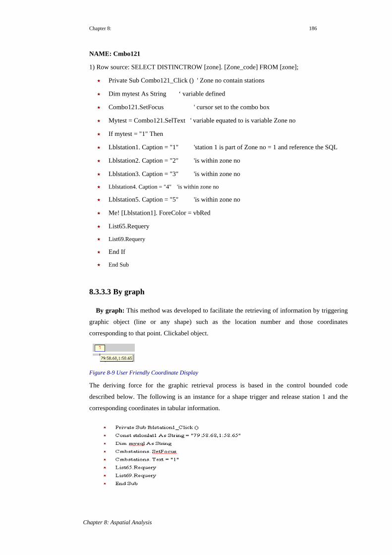
Chapter 8: 186


NAME: Cmbo121

1) Row source: SELECT DISTINCTROW [zone]. [Zone_code] FROM [zone];

Private Sub Combo121_Click () ' Zone no contain stations

Dim mytest As String ‘ variable defined

Combo121.SetFocus ' cursor set to the combo box

Mytest = Combo121.SelText ' variable equated to is variable Zone no

If mytest = "1" Then

Lblstation1. Caption = "1" 'station 1 is part of Zone no = 1 and reference the SQL

Lblstation2. Caption = "2" 'is within zone no




Me! [Lblstation1]. ForeColor = vbRed

List65.Requery

List69.Requery

End If

End Sub

8.3.3.3 By graph

By graph: This method was developed to facilitate the retrieving of information by triggering

graphic object (line or any shape) such as the location number and those coordinates

corresponding to that point. Clickabel object.

Figure 8-9 User Friendly Coordinate Display

The deriving force for the graphic retrieval process is based in the control bounded code

described below. The following is an instance for a shape trigger and release station 1 and the

corresponding coordinates in tabular information.

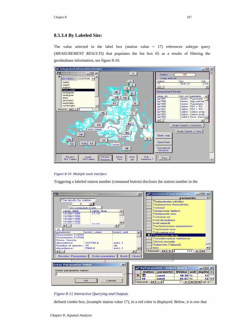
Chapter 8: 187

8.3.3.4 By Labeled Site:

The value selected in the label box (station value = 17) references subtype query

(MEASUREMENT RESULTS) that populates the list box 65 as a results of filtering the

geodatabase information, see figure 8-10.

Figure 8-10 Multiple tools interface

Triggering a labeled station number (command button) discloses the station number in the

Figure 8-11 Interactive Querying and Outputs

defined combo box, (example station value 17), in a red color is displayed. Below, it is row that


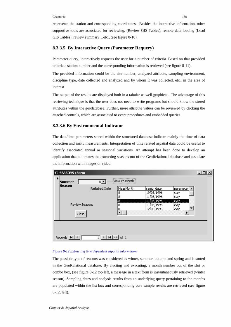
Chapter 8: 188

represents the station and corresponding coordinates. Besides the interactive information, other

supportive tools are associated for reviewing, (Review GIS Tables), remote data loading (Load

GIS Tables), review summary…etc., (see figure 8-10).

8.3.3.5 By Interactive Query (Parameter Requery)

Parameter query, interactively requests the user for a number of criteria. Based on that provided

criteria a station number and the corresponding information is retrieved (see figure 8-11).

The provided information could be the site number, analyzed attribute, sampling environment,

discipline type, date collected and analyzed and by whom it was collected, etc., in the area of

interest.

The output of the results are displayed both in a tabular as well graphical. The advantage of this

retrieving technique is that the user does not need to write programs but should know the stored

attributes within the geodatabase. Further, more attribute values can be reviewed by clicking the

attached controls, which are associated to event procedures and embedded queries.

8.3.3.6 By Environmental Indicator

The date/time parameters stored within the structured database indicate mainly the time of data

collection and insitu measurements. Interpretation of time related aspatial data could be useful to

identify associated annual or seasonal variations. An attempt has been done to develop an

application that automates the extracting seasons out of the GeoRelational database and associate

the information with images or video.

Figure 8-12 Extracting time dependent aspatial information

The possible type of seasons was considered as winter, summer, autumn and spring and is stored

in the GeoRelational database. By electing and executing, a month number out of the slot or

combo box, (see figure 8-12 top left, a message in a text form is instantaneously retrieved (winter

season). Sampling dates and analysis results from an underlying query pertaining to the months

are populated within the list box and corresponding core sample results are retrieved (see figure

8-12, left).


Chapter 8: 189

8.3.4 Correlative Interpretation by Trend Graph type

A cross tap type query result is used to generate the trend graph in association with aggregate

function and a VB specific

function linked with relevant

Timer event procedure. A Line

graph shows the rising and

falling trends among several

data values as indicated below.

For instance invoking a trend button displays graphically the heavy metals trend information. The

application also display the magnitude of the concentration of the heavy metals as SAFE and

UNSAFE, by calculating and comparing internally the values of the measured elements to a

constant attribute values, see figure 8-13.

Figure 8-13 An automated trend analysis and message display


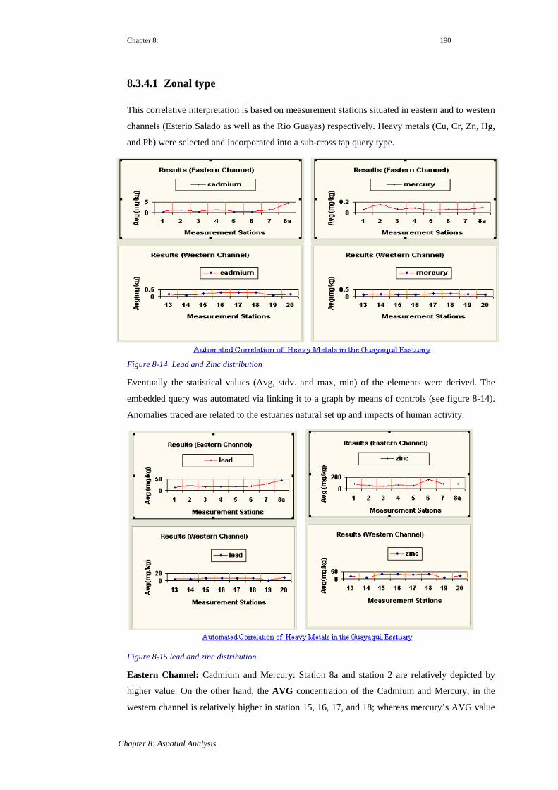
Chapter 8: 190

8.3.4.1 Zonal type

This correlative interpretation is based on measurement stations situated in eastern and to western

channels (Esterio Salado as well as the Rio Guayas) respectively. Heavy metals (Cu, Cr, Zn, Hg,

and Pb) were selected and incorporated into a sub-cross tap query type.

Figure 8-14 Lead and Zinc distribution

Eventually the statistical values (Avg, stdv. and max, min) of the elements were derived. The

embedded query was automated via linking it to a graph by means of controls (see figure 8-14).

Anomalies traced are related to the estuaries natural set up and impacts of human activity.

Figure 8-15 lead and zinc distribution

Eastern Channel: Cadmium and Mercury: Station 8a and station 2 are relatively depicted by

higher value. On the other hand, the AVG concentration of the Cadmium and Mercury, in the

western channel is relatively higher in station 15, 16, 17, and 18; whereas mercury’s AVG value


Chapter 8: 191

is displayed by less than 0.25 mg/kg in the western channel. Hooking a cross tab query to an

event procedure Timer, and changing zone parameter from western to eastern or vice versa

graphically display heavy metals concentration results displayed automatically (see figures15.)

The automated correlation results displays that, in both channels the concentration of zinc is

anomalously detected and is associated to the contaminated emission from the surrounding

galvanic industry.

8.4 Results and Conclusions

Retrieving and filtering important informative issues from the underlying geodatabase requires

know-how of SQL (Structured Query Language), which is an important component in the

exploitation of the constructed GIS. Different executable queries types such as -Parameter query

sub-query and cross tab queries were designed, associated to underlying programs.

By embedding database specific query types such as the TSQ (Transform query) with Visual

Basic (VB) program procedures that link user-friendly interface controls to the underlying

Geodatabase, an interface has been developed.

As a result of the aspatial interface, it was possible to execute many related actions on the

underlain database. Some of which are (a) user friendly process of retrieving information from

database tables, (b), communicate the underlying geodatabase tabular information graphically and

link to spatial engines) (c), display thematical results in an object-control based interface (d)

Locate the processed database information on map-like form interface (e) System-Time linked

automated graphic correlation of measurement results and related message displays.

Furthermore, it was possible to carry out an automated distribution graphic correlation of the

selected heavy metals in the different estuary channels; for instance visualizing the average

dissemination of Zn (zinc) on the eastern as well as western channels of the estuary on the

different measurement stations (see figure 8-15).

The developed tool enables to retrieve process and evaluate the information from different

disciplines incorporated in the geodatabase instantly, and distinguish the possible changes on

updated information.


Chapter 9: 192

Chapter 9: Recapitulations and Suggestions


9.1. Recapitulations

GIS’s potency is based on in its capability to integrate and analyze the organized multidisciplinary

environmental data spatially. With this regard, the need of designing and modeling of a geodatabase

are considered appropriately. Moreover, approaches of GIS application and methodology of organizing

diverse coastal raw data for constructing a functional geodatabase are described and graphically

illustrated.

Main emphasis is given to the Construction of Multidisciplinary Object-Relational Data Model

conceptual entities communication rules, on the bases of a feature class representation as a Non

Lexical Object Types (NOLOT) and Lexical object types (LOT).

To avoid redundancy, enhance spatial and non spatial integrity and reduce multiple spatial joins, a

method of amalgamating multidisciplinary entities belonging to different disciplines is developed. This

has been achieved by objects layering process through adherence of the common property, method,

type and dimensions of the objects.

Furthermore, a master Entity Measurement-Location composed of a set of geospatial coordinates and

migrating spatial pointer is constructed to reference any entity encapsulated within an amalgamated

objects. Physical Implementations of the GeoRelational database entities; including that of enforcing

referential integrity and indexing have been achieved by applying DDL and DAO.

Likewise, feature data sets (points, lines and polygons) were defined and generated using graphic

programs with the spatial engines. On this research work, Geographic Objects and relevant Meta data

were created based on georeferencing-coordinates-bearing data-files (event tables) and operating

macro digitizing.

Well-designed GIS project is vital since it is a chamber for integrating and piecing together of system

application tools; user defined tabular entities, geometric objects, topological operations and

association of geographic objects. Seed files of 2D or 3D types and related geographic objects with

respect to the properties and symbology of feature are created in a hierarchical pattern within a GIS

project. Such practical implementation is illustrated as Category => Marine Map (MP) > MP features

> MP features name > MP features name display order. Furthermore, features are indexed so that

spatial association validation is executed based on the fact that a centroid is associated only once to its

own attachable attribute values. Implementing the process strengthened the objects topological

Chapter 9 193

relationship and integrity of spatial information. Moreover, this process has been vital in clearing any

impediment of smooth interoperability between or among GIS applications.

The Object Relational (OR) GIS data model constructed is suitable and flexible for treating complex

data and it extends (RDBMS) possibility of defining and storing objects, implements both standard

SQL and SQL.x, integrate user defined functions, implement spatial operators to display and perform

spatial analysis by interacting and matching geographic objects.

The structure of Object relational is composed of ObjID, Georeferencing data source and multiple

attributes. Each object could have a specific method and property associated with it. For instance Point

Object method: PLACE POINT is a method for generating a point based on x and y coordinates.

Likewise, PLACE LINE generates geometric object line based on the coordinates of x, y and x1 and y1.

Furthermore, the relationship among objects has been implemented based objects relationship

example, for a Point object inside a polygon; the relationship is Point object CONTAINED WITHIN a

polygon or object polygon contains point object…etc.

GIS map is unique in its application due to the fact that every cited and processed data is geo-

reference-able and topologically related. Research maps georeferencing was carried out applying a

provided ellipsoid and datum of the area INTL–1924 and PSAD56 respectively.

3d Visualization has been executed by increasing the density of observation points (x, y, and z) along a

profile on bathymetric map (estuary) and the tabular data has been processed to generate 3d view of

the area.

Interoperability experiments among different spatial engines reveal loss of some spatial properties

(E.g. shape altered to polyline and projected features to non-projected) during the exchange of

geographic features between non Open GIS complaint and open GIS complaints applications.

The extracting of spatial information has been executed by introducing object-relational and statistical

queries on the developed GIS Geodatabase. Spatial query requires knowledge of (a) feature data set

and topological relationship, (b) sharing matching coordinate system and (c) topological cleanness.

Furthermore, two important aspects are considered to perform the spatial operations, (i) Compatibility

of Matching Rows and (ii) Interactivity of the Object themselves, as indicated in the example below.

� (a) ObjA.FID = ObjB.FID: - extracts all matching objects’ contents

� (b) ObjA ObjB: - extracts all objects topologically related’ contents

� (c) ObjA ObjB: - Extracts objects common,

� (d) ObjA contains ObjB or ObjB within ObjA …etc.


Chapter 9


194

Base on this object relational spatial analysis, it was possible to achieve results related to: -

� a) Identify channels, which disclose abnormality of heavy metals,

� b) Retrieve Lithology extension sheared by tectonics,

� c) Disclose the GeoTectonic trending dissecting different coastal Lithologies.

� d) Reveal thematical variation of temperature within the estuary

� e) Understanding Tidal pattern on the different channels velocity and direction

According to the overlay spatial analysis results of the coastal area image map and vectorised features,

the possible anthropological impacts and processes of submarine erosion pressure are thematically

visualized close to the southern periphery of the estuary. This overlay analysis implies that the

dimension of the southwest estuary water body may extend further northward and the southern island

might submerge as a repercussion of submarine and human dynamism.

Spatio-temporal analysis related to the tidal current velocity and direction, performed on the highly

scattered measurement stations unveiled a certain relationship between the current velocity and the

depth of measurement environment. In this case, the highest and lowest measurement depth points are

associated with lower flood and ebb tide current velocity.

The plausible reason suggested to such phenomenon is likely to be of morphological changes of the

estuary channel at depth, weakening of the current velocity due to friction at top water surface and due

oscillation of the tide generating force (TF) at the sites of measurements during the rise and fall of the

tidal levels..

Chapter 9 195

9.2. Suggestions

System Applications: - The constructed and implemented Geodatabase model has been designed to

deal with the management of multidisciplinary coastal / marine environmental problems. However, it

is also open to be utilized in challenging spatial problems related to continental surface and subsurface

areas.

Data sites: - The lateral distribution of the measurement stations, incorporated in the designed

geodatabase are few and sporadically dispersed. This fact has created a sense of constraint in

generating continuous zone of thematic interpretation. Increasing the measurement density and

integrating with historical data might lead to a better spatially visible result.

Interface: During this research, the geodatabase has been implemented with different GIS

applications. Nonetheless, an aspatial interface has been developed to exploit the underlying

geodatabase pool in a user-friendly manner. .

Raster GIS development: The implemented geodatabase objects are mainly of vector GIS type.

Relevant raster files (satellite images /scanned paper maps) were vectorised, topologically cleaned, and

spatio-temporally integrated. This was an essential step to sort out spatio-temporal problems and

suggest solutions related to coastal environment. However, developing a full-fledged raster and

remote sensing coupled with feature based GIS can be a major theme and task in challenging issues

concerning: -

Identifying areas of higher priorities and Diagnose environmental impacts

Perform remote aerial exploration and prospecting

Detect, Identify and Delineate source of economically viable deposits intended to the advantage

and development of societal wellbeing.


-196-

Appendixes and References

Appendix1 1 Geodatabase Application structure..................................................197 Appendix1 2 Executable Spatio-temporal Query ..................................................199 Appendix1 3 GIS Database Terminology ..............................................................204 Appendix1 4 Geographic Objects Generation (A, B, C, D and E) ........................207 Appendix1 5 Building Aspatial Interface Embedded Program .............................213 References .............................................................................................................218

- 197 -

Appendix 1: GeoDatabase Application Structure

Create table ZONE ( Create table ESTUARY(MSLINK integer UNIQUE, MSLINK integer,MAPID integer NOT NULL, MAPID integer,Zone_code integer CONSTRAINT pkMSLINK PRIMARY KEY, Estation text (6) Constraint PKEst PRIMARY KEY,Zone_locality TEXT (30)); zone_code integer REFERENCES ZONE(zone_code) ,

Create table LOCATION ( LonDegTxt text (10),MSLINK integer UNIQUE, LonDegTxt text (10),MAPID INTEGER NOT NULL, LonDegDec float,Station text (5) CONSTRAINT pkST PRIMARY KEY, LatDegDec float,LonDegTxt text (10), EastingKm float,LatDegTxt text (10), NorthingKm float,LonDegDec float, Area float,LatDegDec float, Perimeter float );EastingKm float, Create table LITHOLOGY(NorthingKm float, MSLINK integer,Area float, MAPID integer,Perimeter float, Georef integer CONSTRAINT Pkgeoref PRIMARY KEY,zone_code integer REFERENCES ZONE (zone_code)); zone_code integer References zone (zone_code),

create table CAMPDATE( LonDegTxt text (10),Dtcode integer CONSTRAINT pkDtcode PRIMARY KEY, LonDegTxt text (10),MSLINK integer, LonDegDec float,mapid integer, LatDegDec float,Station text (6) REFERENCES Location (station), EastingKm float,Samp_date date, NorthingKm float,Samp_time_st date, Area float,Samp_time_e date); Perimeter float,

StratgraphicName text (20),create table FIELD( Lithocomposition text (50)

MSLINK integer,mapid integer, Create table TECTONICSTRUCTURE(Dtcode integer REFERENCES campdate (dtcode), MSLINK integer,Field_code text (6) CONSTRAINT pkFcode PRIMARY KEY, MAPID integer,discipline_name TEXT(25), Georef integer CONSTRAINT Pkgeoref PRIMARY KEY,Environment TEXT (25), zone_code integer References zone (zone_code),Samp_technique TEXT (25), LatDegTxt text (10),Samp_doc TEXT (25), LonDegTxt text (10),Samp_weight_kg FLOAT, LonDegDec float,Samp_volume_m3 FLOAT, LatDegDec float,Samp_volume_l FLOAT); EastingKm float,

create table RESULTS( NorthingKm float,MSLINK integer, Area float,mapid integer, Perimeter float,zone_code integer REFERENCES ZONE (ZONE_CODE) , Trend text (10));Station text (6) REFERENCES LOCATION (STATION), Create table DISCIPLINES(Dtcode integer REFERENCES campdate (dtcode), Discp_code text (6) CONSTRAINT pkdscpcd PRIMARY KEY,Field_code TEXT (6) REFERENCES FIELD (field_code), Station text (6) REFERENCES Location (station),Parameter text (15), Discp_zone_code text (20),Meas_doc text (25), Discp_Name text (30),Meas_doc text (25), Zone_code integer REFERENCES ZONE (zone_code));Pract_value float,Pract_unit text (6), Create Unique Index Locmslink On Location (Mslink Asc); SI_value float, Create Unique Index Tecgeoref On Tectonicstructure (Tgeorefno Asc);SI_unit text (6), Create Unique Index Lgeoref On Lithology (Lgeorefno Asc);Precision float, Create Unique Index Estation On Estuary (Estation Asc);Samp_depth_m float, Create Unique Index Discpcode On Disciplines (Discp_Code Asc);Echo_depth_m float, Create Unique Index Fldcd On Field (Field_Code Asc);Abs_depth_m float, Create Unique Index Cmpdt On Campdate (Dtcode Asc);Meas_code text (15) CONSTRAINT Pkmcod PRIMARY KEY); Create Unique Index Zncd On Zone (Zone_Code Asc);

Create Unique Index Meas-No On Results (Meas_Code Asc);

User Defiend Entities

Geodatabase development Processes

- 198 -

System Generated EntitiesCreate table FEATURE( Create table UGJOIN_CAT(

MSLINK Integer, Jtype Smallint,Fcode Char(12), Table0 char (36),Fname Char (32), Index0 char (36),Category Integer, Table1 char (36),Tablename Char (18), Index1 char (36),Ftype Smallint, Value1 char (36),Flevel Smallint, Descr char (80));Fstyle Smallint, Fweight Smallint, Create table UGTABLE_CAT(Fcolor Smallint, Tname char (128),Digcmd Char (240), Talias char (32),Felement Smallint, Pkey char (32),Fangle Char (16), Descr char (80),Fheight Float, Ustn Smallint);Fwidth Float, Flinespace Float, Create table UGFEATURE(Linelength Smallint, Feature integer,Ffont Smallint, Elock Smallint,Fsymbol Char (1), Fclass SmallintFjustification Char (3), Fpriority Smallint,Celllibrary Char (14), Infomode Smallint,Fcellname Char (6), Das Smallint,Cellscale Float, Dprio integer,Streamdelta Float, Fodder char (16),Streamtolerance Float, Descr char (132),Streamunit Char (15), LsScale float,Snaptype Smallint, DashScale float,Snaptolerance Smallint, GapScale float,Newdup Smallint); StartWidth float,

Create table MSCATALOG( EndWidth float,Tablename char (32), Phase float,Entity integer); Phasetype Smallint, Create table category ( Slant float,MSLINK integer, Cs float,Cname char (32), Underline Smallint,Indexname char (14), Vertical Smallint,Indexlevel Smallint); Fraction Smallint,

Create tableUGCATEGORY ( LsName char (64));Category integer,Defaultf integer, Create tableUGCOMMAND(Olap Smallint, Feature integer,Foreign Smallint, Cname char (32),Dgnfex char (3)); Keyincmd char (240),

create table MAPS ( Sqlstmt char (240),MSLINK integer, Class Smallint );Category integer, Create Unique Index Mscatalog tname on Mscatalog (tablename);Mapname char (14)); Create Unique Index mscatalog_enum on Mscatalog (entitynum);

Create table UGMAP( Create Unique Index category_msl on category (MSLINK);

MAPID integer, Create Unique Index ugcategory_msl on ugcategory (category);Mdir char (128), Create Unique Index ugfeature_msl on ugfeature (feature);Descr char (132), Create Unique Index ugcommand_feanam on ugcommand (feature, name);Viewrot float, Create Unique Index feature_msl on Feature (MSLINK);

Filesize integer); Create Unique Index ugcategory_msl on ugcategory (category);Create Unique Index ugfeature_msl on ugfeature (feature);


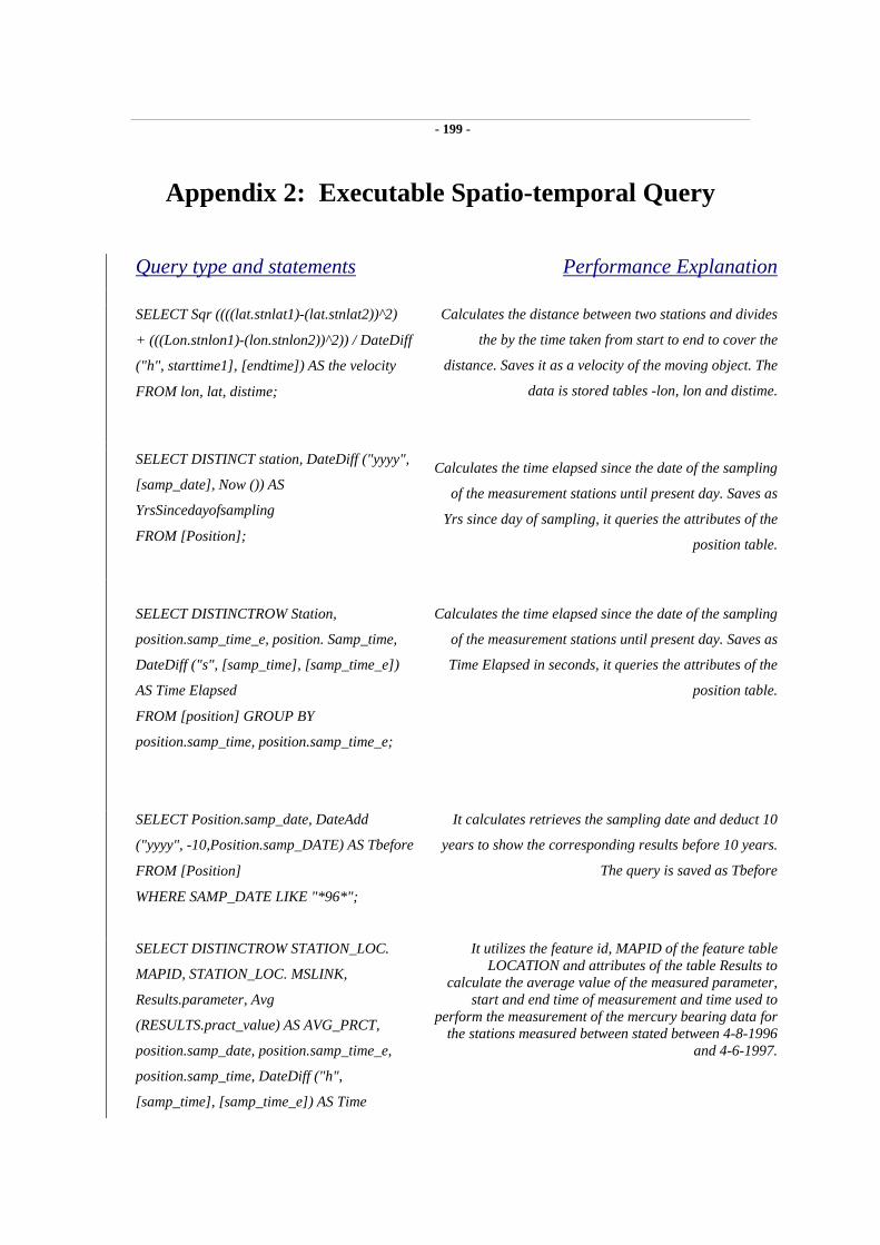
- 199 -

Appendix 2: Executable Spatio-temporal Query

Query type and statements Performance Explanation

SELECT Sqr ((((lat.stnlat1)-(lat.stnlat2))^2)

+ (((Lon.stnlon1)-(lon.stnlon2))^2)) / DateDiff

("h", starttime1], [endtime]) AS the velocity

FROM lon, lat, distime;

Calculates the distance between two stations and divides

the by the time taken from start to end to cover the

distance. Saves it as a velocity of the moving object. The

data is stored tables -lon, lon and distime.

SELECT DISTINCT station, DateDiff ("yyyy",

[samp_date], Now ()) AS

YrsSincedayofsampling

FROM [Position];

Calculates the time elapsed since the date of the sampling

of the measurement stations until present day. Saves as

Yrs since day of sampling, it queries the attributes of the

position table.

SELECT DISTINCTROW Station,

position.samp_time_e, position. Samp_time,

DateDiff ("s", [samp_time], [samp_time_e])

AS Time Elapsed

FROM [position] GROUP BY

position.samp_time, position.samp_time_e;

Calculates the time elapsed since the date of the sampling

of the measurement stations until present day. Saves as

Time Elapsed in seconds, it queries the attributes of the

position table.

SELECT Position.samp_date, DateAdd

("yyyy", -10,Position.samp_DATE) AS Tbefore

FROM [Position]

WHERE SAMP_DATE LIKE "*96*";

It calculates retrieves the sampling date and deduct 10

years to show the corresponding results before 10 years.

The query is saved as Tbefore

SELECT DISTINCTROW STATION_LOC.

MAPID, STATION_LOC. MSLINK,

Results.parameter, Avg

(RESULTS.pract_value) AS AVG_PRCT,

position.samp_date, position.samp_time_e,

position.samp_time, DateDiff ("h",

[samp_time], [samp_time_e]) AS Time

It utilizes the feature id, MAPID of the feature table LOCATION and attributes of the table Results to

calculate the average value of the measured parameter, start and end time of measurement and time used to

perform the measurement of the mercury bearing data for the stations measured between stated between 4-8-1996

and 4-6-1997.

- 200 -


Elapsed, STATION_LOC.station

FROM [position], STATION_LOC, RESULTS

WHERE

(((STATION_LOC.station)=[POSITION].

[STATION])

AND ((POSITION.rec_no)=[RESULTS].

[REC_NO])

AND ((Results.parameter)="MERCURY")

AND ((position.samp_date) Between #4/8/96#

And #4/6/97#))

GROUP BY STATION_LOC. MAPID,

STATION_LOC. MSLINK, Results.parameter,


position.samp_time, STATION_LOC.station;

SELECT DISTINCT Position.samp_date,

Count (Position.samp_time) AS

CountOfsamp_time

FROM [Position] GROUP BY

Position.samp_date;

Counts the number of measurement dates for collecting

the GIS project data from a single table.

TRANSFORM Avg (SUBQUERY1.pract_value)

AS AvgOfpract_value

SELECT SUBQUERY1.parameter

GROUP BY SUBQUERY1.parameter

PIVOT SUBQUERY1.station;

Creates a spreadsheet like table for the average values of

the attribute values of the attribute named parameter.

SELECT STATION_LOC.station,

station_loc.lat, meas_doc, station_loc.lon,

POSITION.samp_time,

POSITION.samp_depth_m, POSITION.rec_no,

RESULTS.rec_no, RESULTS.parameter,

RESULTS.pract_value

FROM station_loc, POSITION, RESULTS

WHERE station_loc.station =

JOIN and UNION Query type

The query process and retrieves information based on the

defined SQL statements.

The three attribute names processed are meas_doc

values, station number, sampling time, sampling depth in

meters, rec-number and the name of the parameter, value

of the parameter retrieved from station_loc and Position

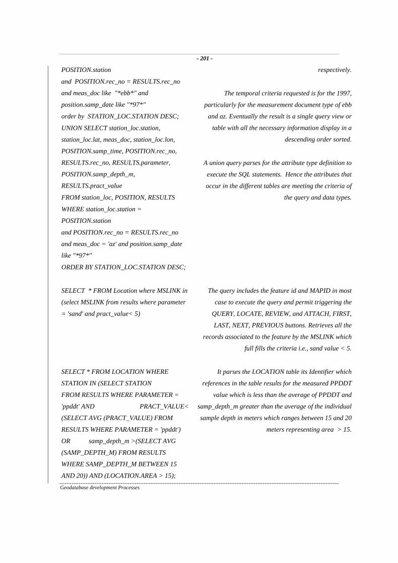
- 201 -


POSITION.station

and POSITION.rec_no = RESULTS.rec_no

and meas_doc like "*ebb*" and

position.samp_date like "*97*"

order by STATION_LOC.STATION DESC;

UNION SELECT station_loc.station,

station_loc.lat, meas_doc, station_loc.lon,

POSITION.samp_time, POSITION.rec_no,

RESULTS.rec_no, RESULTS.parameter,

POSITION.samp_depth_m,

RESULTS.pract_value

FROM station_loc, POSITION, RESULTS

WHERE station_loc.station =

POSITION.station

and POSITION.rec_no = RESULTS.rec_no

and meas_doc = 'az' and position.samp_date

like "*97*"

ORDER BY STATION_LOC.STATION DESC;

respectively.

The temporal criteria requested is for the 1997,

particularly for the measurement document type of ebb

and az. Eventually the result is a single query view or

table with all the necessary information display in a

descending order sorted.

A union query parses for the attribute type definition to

execute the SQL statements. Hence the attributes that

occur in the different tables are meeting the criteria of

the query and data types.

SELECT * FROM Location where MSLINK in

(select MSLINK from results where parameter

= 'sand' and pract_value< 5)

The query includes the feature id and MAPID in most

case to execute the query and permit triggering the

QUERY, LOCATE, REVIEW, and ATTACH, FIRST,

LAST, NEXT, PREVIOUS buttons. Retrieves all the

records associated to the feature by the MSLINK which

full fills the criteria i.e., sand value < 5.

SELECT * FROM LOCATION WHERE

STATION IN (SELECT STATION

FROM RESULTS WHERE PARAMETER =

'ppddt' AND PRACT_VALUE<

(SELECT AVG (PRACT_VALUE) FROM

RESULTS WHERE PARAMETER = 'ppddt')

OR samp_depth_m >(SELECT AVG

(SAMP_DEPTH_M) FROM RESULTS

WHERE SAMP_DEPTH_M BETWEEN 15

AND 20)) AND (LOCATION.AREA > 15);

It parses the LOCATION table its Identifier which

references in the table results for the measured PPDDT

value which is less than the average of PPDDT and

samp_depth_m greater than the average of the individual

sample depth in meters which ranges between 15 and 20

meters representing area > 15.

- 202 -



STATION IN (SELECT STATION FROM

RESULTS WHERE PARAMETER = 'lead'

AND PRACT_VALUE> (SELECT AVG

(PRACT_VALUE) * 2 FROM RESULTS

WHERE PARAMETER = 'lead') AND

samp_depth_m > (SELECT AVG


WHERE SAMP_DEPTH_M BETWEEN 0 AND

5)) AND (LOCATION.AREA > 5);

Select all the attributes in the Location table and

reference the station attributes to the station in the table

results. The parameter LEAD is selected and compared

ageist all those greater than 2 times average and

samp_depth_m is compared to that greater than average

forrange depth between 0 and 5 for area greater than 5.


STATION IN (SELECT STATION

FROM RESULTS WHERE PARAMETER =

'ppddt' AND pract_value <

(SELECT AVG (PRACT_VALUE) FROM

RESULTS WHERE PARAMETER = 'ppddt')

OR samp_depth_m >(SELECT AVG


WHERE SAMP_DEPTH_M BETWEEN 15

AND 20)) AND (LOCATION.AREA > 15);

It parses the LOCATION table its Identifier which

references in the table results for the measured PPDDT

value which is less than the average of PPDDT and

samp_depth_m greater than the average of the individual

sample depth in meters which ranges between 15 and 20

meters representing area > 15.


STATION IN (SELECT STATION FROM

RESULTS WHERE PARAMETER = 'salinity'

AND pract_value < (SELECT AVG

(pract_value) FROM RESULTS WHERE

PARAMETER = 'salinity') AND

samp_depth_m > (SELECT AVG


WHERE samp_depth_m BETWEEN 0 AND

15)) AND (LOCATION.AREA >5);

Retrieves locations where salinity less than the averages

and samp_dep_m is less than the average depth per

station only for the depth between 0 and 15 m and

locational area > 5 sq km.

- 203 -


PARAMETER [Beginning Date] DateTime,

[Ending Date] DateTime;

SELECT DISTINCTROW POSITION.station,

Format (samp_Date,"dd-mm-yyyy") AS [Year],

Format$(samp_time,"hh:nn:ss") AS MTime,

Results.parameter, RESULTS.pract_value,

results.SI_value

FROM [position], results

WHERE (((Results.parameter)="sand") AND

((POSITION.rec_no)=[results]. [Rec_no])

AND ((position.samp_date) Between

[Beginning Date] And [Ending Date]));

It requests the user the beginning date and ending date of

measurement, then selects the stations, measured

attributes and the value of analysis from the position and

results tables respectively. The value of the attribute is

equated to sand for the data only for those between the

beginning and ending date. The final results are

displayed in format as Mtime for the sampling time and

as a Year for the sampling year.

SELECT DISTINCTROW STATION_LOC.

MAPID, STATION_LOC.MSLINK,

RESULTS.parameter,

Results.pract_unit, Max

(RESULTS.pract_value) AS AVG_PRCT,


position.samp_time, DateDiff ("s",

[samp_time], [samp_time_e])/60 AS Time

Elapsed, STATION_LOC.station,

Station_Loc.lon, Station_Loc.lat

FROM [position], STATION_LOC, RESULTS

WHERE

(((STATION_LOC.station)=[POSITION].

[STATION]) AND

((POSITION.rec_no)=[RESULTS].

[REC_NO]) AND

((RESULTS.parameter)="MERCURY") AND

((Position.samp_date) Between #4/8/1996#

And #4/6/1997#))

GROUP BY STATION_LOC. MAPID,

STATION_LOC.MSLINK,

RESULTS.parameter, Results.pract_unit,


Calculates the measured values of mercury between the

time elapsed for measurement 1 and measurement 2 in

terms of minutes The search of the data includes three

tables in which the Master table is associated with spatial

features and checks for all samples which have last

measurement time represented by measurement

samp_time_e.

- 204 -


position.samp_time, STATION_LOC.station,

Station_Loc.lon, Station_Loc.lat

HAVING (((position.samp_time_e) Is Not

Null));

SELECT samp_date, DateDiff ("yyyy", now (),

samp_date) AS time difference

FROM [position];

Retrieves the information between the present and date of

measurements

Appendix 3: GIS Database Terminology

Term MeaningATTRIBUTE It is a column name that describe a specific entity

GEORELATIONAL_TABLE An out put of an associated attribute and feature tables

DDL An acronym for data definition language used by SQL

DML An acronym for data manipulation language used by SQL Statement to define

the database components

ENTITY Table related to its affiliated attributes

NOLOT Non Lexical Object (Entity)

LOT Lexical objects (attribute)

DATABASE DESIGN A process where the conceptually established data model is implemented in a

specific database.

RELATIONAL JOIN The relating of two or more tables in a relational database on the basis of a

common item or field

LINKED TABLE A Table or flat file linked to a database for viewing or editing

DATA TYPE Data type a reference to the type of an attribute’s content. For instance to

handle numerals as numbers or simply as character data and are utilized in

ensuring data integrity within a database.

NORMALIZATION A process in a data modeling method used as a database design tool for

relational databases.

3NF Every attribute is unique + pk, + non transitively - dependent on the pk

2NF Every attribute is unique + functionally dependent on pk

1NF Every attribute is unique

CREATE TABLE Defining the database table components using a data definition language

INSERT INTO An SQL statement function used to populate a table using the SELECT data

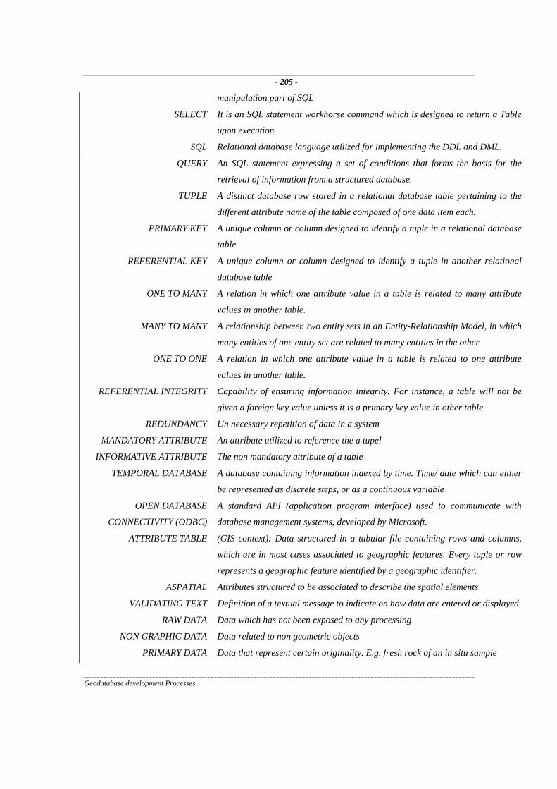
- 205 -


manipulation part of SQL

SELECT It is an SQL statement workhorse command which is designed to return a Table

upon execution

SQL Relational database language utilized for implementing the DDL and DML.

QUERY An SQL statement expressing a set of conditions that forms the basis for the

retrieval of information from a structured database.

TUPLE A distinct database row stored in a relational database table pertaining to the

different attribute name of the table composed of one data item each.

PRIMARY KEY A unique column or column designed to identify a tuple in a relational database

table

REFERENTIAL KEY A unique column or column designed to identify a tuple in another relational

database table

ONE TO MANY A relation in which one attribute value in a table is related to many attribute

values in another table.

MANY TO MANY A relationship between two entity sets in an Entity-Relationship Model, in which

many entities of one entity set are related to many entities in the other

ONE TO ONE A relation in which one attribute value in a table is related to one attribute

values in another table.

REFERENTIAL INTEGRITY Capability of ensuring information integrity. For instance, a table will not be

given a foreign key value unless it is a primary key value in other table.

REDUNDANCY Un necessary repetition of data in a system

MANDATORY ATTRIBUTE An attribute utilized to reference the a tupel

INFORMATIVE ATTRIBUTE The non mandatory attribute of a table

TEMPORAL DATABASE A database containing information indexed by time. Time/ date which can either

be represented as discrete steps, or as a continuous variable

OPEN DATABASE

CONNECTIVITY (ODBC)

A standard API (application program interface) used to communicate with

database management systems, developed by Microsoft.

ATTRIBUTE TABLE (GIS context): Data structured in a tabular file containing rows and columns,

which are in most cases associated to geographic features. Every tuple or row

represents a geographic feature identified by a geographic identifier.

ASPATIAL Attributes structured to be associated to describe the spatial elements

VALIDATING TEXT Definition of a textual message to indicate on how data are entered or displayed

RAW DATA Data which has not been exposed to any processing

NON GRAPHIC DATA Data related to non geometric objects

PRIMARY DATA Data that represent certain originality. E.g. fresh rock of an in situ sample

- 206 -


SECONDARY DATA Resampled data. E.g. converting paper map to electronic file for building the

GIS

SYSTEM GENERATED

ENTITIES

Special tables generated by the spatial engine to work coherently with an

external data model

USER DEFINED ENTITIES Structured relational database tables which could be joined to system generated

tables by means a migrating key

MEASURED_RESULTS Multidisciplinary data structured systematically to have a common a common

identifiers for easy access and retrieval process

LITHOLOGY-DATA Raw data related to geologically distinctive lithologic attributes

TECTONIC-DATA Attributes related to the tectonic structure for instance, fault trends, strike and

dip angles

CAMPAIGNDATEDATA An entity composed mainly of temporal parameters

LOCATION-DATA An entity containing georefrencing data sources

AMALGAMATION The fusing of different structured tables to reduce the number join tables and

facilitate the retrieving (a process of demoralization)

CASCADE UPDATES The possibility to enable a referential integrity constraint changes despite the

defined referential integrity to update

CASCADE DELETIONS The possibility to enable a referential integrity constraint changes despite the

defined referential integrity to delete

SPATIAL BUILDING BLOCK

ENTITIES

Entities that compose the GIS associated feature tables.

SQL SYNTAX DIFFERENCE The difference of utilizing SQL statement to return values in form a query view.

INDEXING A process of creating keys that helps to increase the speed of accessing and

retrieving the data

HIERARCHICAL DATA STR.

(HDS)

The data model is based on the required constraint that a child record is not

supported to have a multiple parents. Hierarchical data models represent data

in a tree like structure, with one data type providing the root (initial map) to

which all others are linked via parent/child relationships with hidden pointer.

NETWORK DATA STRU.

(HDS)

Network data model were constructed to compensate the weakness of a

hierarchical model by allowing different parents to point to a single child or a

child point to a different parents

RELATIONAL DATA STRU.

(RDS)

A relational database model based on tables (relations), fields and rows.

Operations based on structured tables are easily implemented based on common

values that can be easily corrected and identified in case of system failures.

DATABASE The possibility and ability of different software systems to exchange information

- 207 -


COMMUNICATION and requests, using methods such as object linking or translation of different

feature.

NESTED SQL (SUBQUERY) A query that reference a second query by means of IN key word to retrieve

related information

CROSS TAB QUERY Special select type query that output results in a spread sheet format

ASPATIAL ANALYSIS Analysis performed on data stored in an attribute database, without associating

to spatial features

UNION OPERATION A query used to create the union of two or more tables

INTERSECTION A query employed to generate the common attribute values of the two or more

tables

LIST BOX A List display of table's results in a visual basic form

ZONAL CORRELATION Spatial correlation based on different zone in a regional/ local environment

ANOMALIES Abnormal display of certain measured or analyzed values

ENTITY RELATIONAL MODEL A logical way of describing entities and their relationships within relational

databases, in most cases diagrammatically

TRANSFORMATION Process of rectification, typically involves rotation and scaling of grid cells

during a projection system.

Appendix 4: Geographic Objects Generation (A,B,C,D and E)

A Geographic Objects (MapInfo)

Set Obj = Create line (LonDegDec, LatDegDec,

LonDegDec2, LatDegDec2)

Purpose: Create a line object based on the starting

and ending points of coordinates.

Requirements: MapBasic and .tab file (MapInfo GIS)

Specific Projection system (case study PASDA56)

Update LocationPoint

Set Obj = Create Circle (LonDegDec, LonDegDec, Unit)

The Point Object is converted into a circle with a specific

filed radius in U (unit

Purpose: Create a circle object based on

Point and it’s a radius



Update Circle Object

Set obj= Create Point (Centroid (Obj)), (Centroid (Obj))

Purpose: Creates a point by reversing

a circle object into a point.



- 208 -


1. Mslink Integer ; 2. LonDegDec Float ; 3. LatDegDec Float ;

4. Area Float ; 5. Perimeter Float ;

6. Myimage Char (45) ; 7. Begin_Metadata

8. "\Activeobject" = "" 9. "\Activeobject\Expr" = "Myimage"

10. "\Activeobject\Mode" = "Hotlink_Mode_Both" 11. "\Activeobject\Relative" = "True"

12. "\Isreadonly" = "False" 13. End_Metadata

A spatial object and object generating code.Steps 1 defines an object identifier

2 and 3 are coordinates4 and 5 defines possible dimensions of the object

6 variable for the meta data object path7 defines the meta object creations

Requirements:.tab file

MapBasicSpecific projection system

B Geographic object (MBE): Polyline (lstring object)

Defining type and objects Sub Main Dim MaxNorthing As Double Dim MaxEasting As Double Dim scaleNorthing As Double Dim scaleEasting As Double Dim InString As String Dim PointCount As Integer Dim point() As MbePoint Dim ThisPoint As MbePoint Dim I As Intege MbeSendCommand "SUPPRESSED NOECHO" MbeWriteCommand "DRAWING Graph" MbeWriteStatus "Graph on work... MaxNorthing = 0.0 MaxEasting = 0.0 PointCount = 0 'Pointing to the data file Open "path" For Input Access Read As #1 '---------------------------------------------------------------------- ' Reading the Provided values into array ' the loop While NOT EOF(1) Line Input #1, InString thisPoint.X = Val(Item$(inString,1,1,",")) thisPoint.Y = Val(Item$(inString,2,2,",")) PointCount = PointCount + 1 Redim Preserve point(pointCount) point(pointCount) = thisPoint If thisPoint.X > MaxNorthing Then MaxNORTHING = thisPoint.X End If If thisPoint.Y> MaxEasting Then maxEasting = thisPoint.Y End If Wend Close #1 '----------------------------------------------------- scaleNorthing = Northing / MaxNorthing

- 209 -


scaleEasting = Easting / maxEasting 'Scaling the array For I = 1 to pointCount point(i).X = point(i).X * scalenorthing point(i).Y = point(i).Y * scaleeasting Next I 'Drawing the limiting axes MbeSendCommand "PLACE LSTRING SPACE" MbeSendDataPoint 0,7,0 MbeSendDataPoint 0,0,0 MbeSendDataPoint 9,0,0 MbeSendReset 'Generating the GEG Mbesendkeyin "place point" 'MbeSendCommand "PLACE LSTRING SPACE" For I = 1 to pointCount MbeSendKeyin "XY=" + Cstr(point(i).X) + "," + Cstr(point(i).Y) Next I MbeSendReset MbeWritePrompt "" MbeWriteCommand "" MbeWriteStatus "Finished - GEG" MbeSendCommand "ECHO" End Sub

C Geographic Objects : Points and shape on 3d Seed File SUB MAIN Dim startPoint As MbePoint Dim point As MbePoint, point2 As MbePoint MbeSendCommand "ACTIVE COLOR 12" MbeSendCommand "ACTIVE STYLE 0" MbeSendCommand "ACTIVE WEIGHT 0" MbeSendKeyin "place circle radius" MbeSendKeyin "1.2" MbeSendCommand "ACTIVE level 12" Mbesendkeyin"xy=613.928,9781.452,-11.00" ' 1 Mbesendkeyin"xy=628.344,9770.452,-4.000" '4 Mbesendkeyin"xy=625.346,9763.399,-5.500" '2 Mbesendkeyin"xy=626.588,9761.000,-7.000" '3 Mbesendkeyin"xy=624.575,9756.538,-11.000" '5 Mbesendkeyin"xy=626.990,9750.894,-8.000" '6 Mbesendkeyin"xy=630.013,9742.306,-9.600" '6.6 Mbesendkeyin"xy=628.162,9733.231,-12.500" '7 Mbesendkeyin"xy=625.986,9724.401,-8.600" '8A Mbesendkeyin"xy=622.475,9714.884,-7.000" '9A MbeSendKeyin "1.6" Mbesendkeyin"xy=623.991,9698.232,-6.46" '10 Mbesendkeyin"xy=608.492,9706.722,-7.000" '11 MbeSendKeyin "1." Mbesendkeyin"xy=598.066,9704.592,-12.000" '12 Mbesendkeyin"xy=596.181,9704.824,-4.1000" '12A Mbesendkeyin"xy=586.601,9703.875,-13.300" '13 'Mbesendkeyin"xy=582.071,9695.929,-5.500" '13_1 Mbesendkeyin"xy=583.613,9703.875,-3.500" '13A MbeSendKeyin "1.6"

Purpose: Create a an ellipsoid shape around point of measurement

Requirements:3D seed file (MicroStation Environment)

Preferable with a specific Projection (case study SAD1956)

Z value viewer tool (Accurate draw tool.

A Macro that generates point bounded by user defined radius (zone) of interest and measurement depth in a

given unit.A map is generated within a georeferenced grid map

The values of the x, y and z are referenced from within the Geodatabase

The comments characters with the left single quotation mark indicate

A label of the site of interest.

Flexibility: It is possible to modify the symbology of the features and the dimension of the given semi circular

- 210 -


Mbesendkeyin"xy=592.981,9712.216,-13.6000" '14 Mbesendkeyin"xy=604.487,9721.383,-7.000" '15 Mbesendkeyin"xy=608.617,9733.221,-10.700" '16 MbeSendKeyin "1.4" Mbesendkeyin"xy=616.258,9743.769,-19.000" '17 Mbesendkeyin"xy=621.742,9747.027,-14.000" '19 Mbesendkeyin"xy=619.031,9749.013,-17.000" '18 Mbesendkeyin"xy=617.491,9753.064,-19.000" '20 MBESENDRESET mbeSendKeyin "place point" MbeSendCommand "ACTIVE COLOR 10" MbeSendCommand "ACTIVE STYLE 0" MbeSendCommand "ACTIVE WEIGHT 3" MbeSendCommand "ACTIVE level 10" Mbesendkeyin"xy=613.928,9781.452,-11.00" ' 1 Mbesendkeyin"xy=628.344,9770.452,-4.000" '4 Mbesendkeyin"xy=625.346,9763.399,-5.500" '2 Mbesendkeyin"xy=626.588,9761.000,-7.000" '3 Mbesendkeyin"xy=624.575,9756.538,-11.000" '5 Mbesendkeyin"xy=626.990,9750.894,-8.000" '6 Mbesendkeyin"xy=630.013,9742.306,-9.600" '6.6 Mbesendkeyin"xy=628.162,9733.231,-12.500" '7 Mbesendkeyin"xy=625.986,9724.401,-8.600" '8A Mbesendkeyin"xy=622.475,9714.884,-7.000" '9A Mbesendkeyin"xy=623.991,9698.232,-6.46" '10 Mbesendkeyin"xy=608.492,9706.722,-7.000" '11 MbeSendKeyin "1.2" Mbesendkeyin"xy=598.066,9704.592,-12.000" '12 Mbesendkeyin"xy=596.181,9704.824,-4.1000" '12A MbeSendKeyin "1.2" Mbesendkeyin"xy=586.601,9703.875,-13.300" '13 'Mbesendkeyin"xy=582.071,9695.929,-5.500" '13_1 Mbesendkeyin"xy=583.613,9703.875,-3.500" '13A Mbesendkeyin"xy=592.981,9712.216,-13.6000" '14 Mbesendkeyin"xy=604.487,9721.383,-7.000" '15 Mbesendkeyin"xy=608.617,9733.221,-10.700" '16 Mbesendkeyin"xy=616.258,9743.769,-19.000" '17 Mbesendkeyin"xy=621.742,9747.027,-14.000" '19 Mbesendkeyin"xy=619.031,9749.013,-17.000" '18 Mbesendkeyin"xy=617.491,9753.064,-19.000" '20 MBESENDRESET END SUB

values.

The feature point is created and associated to shape geographic element via MbeSendCommand "CREATE

CENTROIDS "MbeSendCommand "FEATURE ATTACH " and provided that the MbeSendCommand "ACTIVE

FEATURE name= Category.featureName.Element type" the database records associated

MbeSendCommand MbeSendCommand "ASSOCIATE LINKAGES "

D Bottom channel morphology Profile Generation SUB MAIN Dim startPoint As MbePoint Dim point As MbePoint, point2 As MbePoint MbeSendCommand "ACTIVE COLOR 12" MbeSendCommand "ACTIVE STYLE 0" MbeSendCommand "ACTIVE WEIGHT 6" MbeSendKeyin "place line" Mbesendkeyin"xy=613.928,9781.452,-11.00" Mbesendkeyin"xy=621.136,9775.952,-7.500" Mbesendkeyin"xy=628.344,9770.452,-4.000" Mbesendkeyin"xy=625.346,9763.399,-5.500" Mbesendkeyin"xy=625.967,9762.203,-6.250" Mbesendkeyin"xy=626.588,9761.000,-7.00" Mbesendkeyin"xy=625.582,9758.772,-9.00"

Purpose: Generates cross sectional profile across the different estuary channels based on the measurements points. Depth

profile visualized by customizing the left, right or front. MicroStaion 3D viewing tools

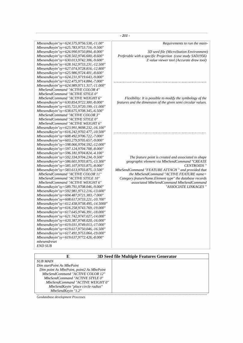
- 211 -


Mbesendkeyin"xy=624.575,9756.538,-11.00" Mbesendkeyin"xy=625.783,9753.716,-9.500" Mbesendkeyin"xy=626.990,9750.894,-8.000" Mbesendkeyin"xy=628.502,9746.600,-8.600" Mbesendkeyin"xy=630.013,9742.306,-9.600" Mbesendkeyin"xy=628.162,9733.231,-12.500" Mbesendkeyin"xy=627.074,9728.816,-12.800" Mbesendkeyin"xy=625.986,9724.401,-8.600" Mbesendkeyin"xy=624.231,9719.643,-9.000" Mbesendkeyin"xy=622.475,9714.884,-7.000" Mbesendkeyin"xy=624.989,9711.317,-11.000" MbeSendCommand "ACTIVE COLOR 4" MbeSendCommand "ACTIVE STYLE 0" MbeSendCommand "ACTIVE WEIGHT 6" Mbesendkeyin"xy=630.854,9722.300,-8.000" Mbesendkeyin"xy=635.721,9720.199,-11.000" Mbesendkeyin"xy=638.675,9708.345,-6.500" MbeSendCommand "ACTIVE COLOR 3" MbeSendCommand "ACTIVE STYLE 0" MbeSendCommand "ACTIVE WEIGHT 6" Mbesendkeyin"xy=623.991,9698.232,-16.100" Mbesendkeyin"xy=616.242,9702.477,-10.500" Mbesendkeyin"xy=608.492,9706.722,-7.000" Mbesendkeyin"xy=603.279,9705.657,-9.000" Mbesendkeyin"xy=598.066,9704.592,-12.000" Mbesendkeyin"xy=597.124,9704.708,-8.000" Mbesendkeyin"xy=596.181,9704.824,-4.100" Mbesendkeyin"xy=592.334,9704.234,-9.500" Mbesendkeyin"xy=586.601,9703.875,-13.300" Mbesendkeyin"xy=585.107,9703.875,-8.000" Mbesendkeyin"xy=583.613,9703.875,-3.500" MbeSendCommand "ACTIVE COLOR 11" MbeSendCommand "ACTIVE STYLE 10" MbeSendCommand "ACTIVE WEIGHT 6" Mbesendkeyin"xy=589.791,9708.046,-9.000" Mbesendkeyin"xy=592.981,9712.216,-13.600" Mbesendkeyin"xy=604.487,9721.383,-7.000" Mbesendkeyin"xy=608.617,9733.221,-10.700" Mbesendkeyin"xy=612.438,9738.495,-14.5000" Mbesendkeyin"xy=616.258,9743.769,-19.000" Mbesendkeyin"xy=617.645,9746.391,-18.000" Mbesendkeyin"xy=621.742,9747.027,-14.000" Mbesendkeyin"xy=620.387,9748.020,-16.000" Mbesendkeyin"xy=619.031,9749.013,-17.000" Mbesendkeyin"xy=619.617,9750.046,-16.500" Mbesendkeyin"xy=617.491,9753.064,-19.000" Mbesendkeyin"xy=619.637,9772.426,-8.000" mbesendreset END SUB

Requirements to run the main-

3D seed file (MicroStation Environment) Preferable with a specific Projection (case study SAD1956)

Z value viewer tool (Accurate draw tool)

………………………………………………………………………….

Flexibility: It is possible to modify the symbology of the features and the dimension of the given semi circular values.

…………………………………………………………………………


CENTROIDS " MbeSendCommand "FEATURE ATTACH " and provided that

the MbeSendCommand "ACTIVE FEATURE name= Category.featureName.Element type" the database records

associated MbeSendCommand MbeSendCommand "ASSOCIATE LINKAGES "

E 3D Seed file Multiple Features Generator

SUB MAIN Dim startPoint As MbePoint Dim point As MbePoint, point2 As MbePoint MbeSendCommand "ACTIVE COLOR 12" MbeSendCommand "ACTIVE STYLE 0" MbeSendCommand "ACTIVE WEIGHT 0" MbeSendKeyin "place circle radius" MbeSendKeyin "1.2"

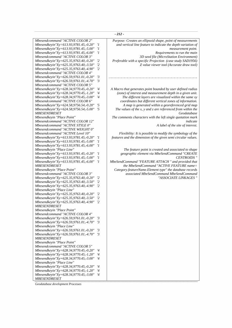
- 212 -


Mbesendcommand "ACTIVE COLOR 2" Mbesendkeyin"Xy=613.93,9781.45,-0.20" '1 Mbesendkeyin"Xy=613.93,9781.45,-5.00" '1 Mbesendkeyin"Xy=613.93,9781.45,-6.00" '1 Mbesendcommand "ACTIVE COLOR 3" Mbesendkeyin"Xy=625.35,9763.40,-0.20" '2 Mbesendkeyin"Xy=625.35,9763.40,-3.50" '2 Mbesendkeyin"Xy=625.35,9763.40,-4.90" '2 Mbesendcommand "ACTIVE COLOR 4" Mbesendkeyin"Xy=626.59,9761.01,-0.20" '3 Mbesendkeyin"Xy=626.59,9761.01,-4.70" '3 Mbesendcommand "ACTIVE COLOR 5" Mbesendkeyin"Xy=628.34,9770.45,-0.20" '4 Mbesendkeyin"Xy=628.34,9770.45,-1.20" '4 Mbesendkeyin"Xy=628.34,9770.45,-3.00" '4 Mbesendcommand "ACTIVE COLOR 6" Mbesendkeyin"Xy=624.58,9756.54,-0.20" '5 Mbesendkeyin"Xy=624.58,9756.54,-5.00" '5 MBESENDRESET Mbesendkeyin "Place Point" Mbesendcommand "ACTIVE COLOR 12" Mbesendcommand "ACTIVE STYLE 0" Mbesendcommand "ACTIVE WEIGHT 0" Mbesendcommand "ACTIVE Level 10" Mbesendkeyin"Xy=613.93,9781.45,-0.20" '1 Mbesendkeyin"Xy=613.93,9781.45,-5.00" '1 Mbesendkeyin"Xy=613.93,9781.45,-6.00" '1 Mbesendkeyin "Place Line" Mbesendkeyin"Xy=613.93,9781.45,-0.20" '1 Mbesendkeyin"Xy=613.93,9781.45,-5.00" '1 Mbesendkeyin"Xy=613.93,9781.45,-6.00" '1 MBESENDRESET Mbesendkeyin "Place Point" Mbesendcommand "ACTIVE COLOR 3" Mbesendkeyin"Xy=625.35,9763.40,-0.20" '2 Mbesendkeyin"Xy=625.35,9763.40,-3.50" '2 Mbesendkeyin"Xy=625.35,9763.40,-4.90" '2 Mbesendkeyin "Place Line" Mbesendkeyin"Xy=625.35,9763.40,-0.20" '2 Mbesendkeyin"Xy=625.35,9763.40,-3.50" '2 Mbesendkeyin"Xy=625.35,9763.40,-4.90" '2 MBESENDRESET Mbesendkeyin "Place Point" Mbesendcommand "ACTIVE COLOR 4" Mbesendkeyin"Xy=626.59,9761.01,-0.20" '3 Mbesendkeyin"Xy=626.59,9761.01,-4.70" '3 Mbesendkeyin "Place Line" Mbesendkeyin"Xy=626.59,9761.01,-0.20" '3 Mbesendkeyin"Xy=626.59,9761.01,-4.70" '3 MBESENDRESET Mbesendkeyin "Place Point" Mbesendcommand "ACTIVE COLOR 5" Mbesendkeyin"Xy=628.34,9770.45,-0.20" '4 Mbesendkeyin"Xy=628.34,9770.45,-1.20" '4 Mbesendkeyin"Xy=628.34,9770.45,-3.00" '4 Mbesendkeyin "Place Line" Mbesendkeyin"Xy=628.34,9770.45,-0.20" '4 Mbesendkeyin"Xy=628.34,9770.45,-1.20" '4 Mbesendkeyin"Xy=628.34,9770.45,-3.00" '4 MBESENDRESET

Purpose: Creates an ellipsoid shape, point of measurements and vertical line feature to indicate the depth variation of

measurement point. Requirements to run the main

3D seed file (MicroStation Environment) Preferable with a specific Projection (case study SAD1956)

Z value viewer tool (Accurate draw tool)

………………………………………………………………………….

A Macro that generates point bounded by user defined radius (zone) of interest and measurement depth in a given unit.

The different layers are visualized within the same xy coordinates but different vertical zones of information.

A map is generated within a georeferenced grid map The values of the x, y and z are referenced from within the

Geodatabase The comments characters with the left single quotation mark

indicate A label of the site of interest.

Flexibility: It is possible to modify the symbology of the

features and the dimension of the given semi circular values.


CENTROIDS " MbeSendCommand "FEATURE ATTACH " and provided that

the MbeSendCommand "ACTIVE FEATURE name= Category.featureName.Element type" the database records

associated MbeSendCommand MbeSendCommand "ASSOCIATE LINKAGES "

- 213 -


Mbesendkeyin "Place Point" Mbesendcommand "ACTIVE COLOR 6" Mbesendkeyin"Xy=624.58,9756.54,-0.20" '5 Mbesendkeyin"Xy=624.58,9756.54,-5.00" '5 Mbesendkeyin "Place Line" Mbesendcommand "ACTIVE COLOR 6" Mbesendkeyin"Xy=624.58,9756.54,-0.20" '5 Mbesendkeyin"Xy=624.58,9756.54,-5.00" '5 MBESENDRESET Mbesendcommand "ACTIVE COLOR 12" Mbesendcommand "ACTIVE STYLE 0" Mbesendcommand "ACTIVE WEIGHT 0" Mbesendkeyin "Place Circle Radius" Mbesendkeyin "1.2" Mbesendcommand "ACTIVE COLOR 2" Mbesendkeyin"Xy=613.93,9781.45,-0.20" '1 Mbesendkeyin"Xy=613.93,9781.45,-5.00" '1 Mbesendkeyin"Xy=613.93,9781.45,-6.00" '1 Mbesendcommand "ACTIVE COLOR 3" Mbesendkeyin"Xy=625.35,9763.40,-0.20" '2 Mbesendkeyin"Xy=625.35,9763.40,-3.50" '2 Mbesendkeyin"Xy=625.35,9763.40,-4.90" '2 Mbesendcommand "ACTIVE COLOR 4" Mbesendkeyin"Xy=626.59,9761.01,-0.20" '3 Mbesendkeyin"Xy=626.59,9761.01,-4.70" '3 Mbesendcommand "ACTIVE COLOR 5" Mbesendkeyin"Xy=628.34,9770.45,-0.20" '4 Mbesendkeyin"Xy=628.34,9770.45,-1.20" '4 Mbesendkeyin"Xy=628.34,9770.45,-3.00" '4 Mbesendcommand "ACTIVE COLOR 6" Mbesendkeyin"Xy=624.58,9756.54,-0.20" '5 Mbesendkeyin"Xy=624.58,9756.54,-5.00" '5 MBESENDRESET end sub

Appendix 5: Building Aspatial Interface Embedded Program Figure 8-8 : Retrieving by station and Zone

Private Sub Combo4_Click() Dim mysql As String mysql = "select attributes from attributes" Dim GISent As String Combo4.SetFocus GISent = Combo4.SelText If GISent = Combo4.SelText Then Combo4.ControlTipText = [Forms]![form3]![Combo4].SelText List6.Requery

- 214 -


End If If List6.Visible = True Then List6.ControlTipText = "selected entity's attributes" List6.ForeColor = vbBlack END SUB

Obj. Name: cobmo4 CONTROL TIP: location ROW SOURCE:

Select Qentities.Entityname From Qentities; Obj.name: Xlist6 ROW SOURCE: SELECT ATTRIbutes.attributes FROM ATTRIbutes WHERE (((ATTRIbutes.entityname)= [forms]![form3]![combo4].[seltext]));

Location coordinate driven results based on label object Obj.Name = lblstation1

Event Procedure: Private Sub lblstation1_Click() Const strlonlat1 As String = "79:58.68,1:58.65" Dim mysql As String cmbstations.SetFocus cmbstations.Text = "1" List65.Requery List69.Requery lblstation1.ControlTipText = strlonlat1 End Sub

name : Cmbstations Row source :

SELECT DISTINCTROW STATION_LOC.station, STATION_LOC.lon, STATION_LOC.lat FROM STATION_LOC;

Obj name List 65 ROW SOURCE:

SELECT DISTINCTROW qrypositionformap.samp_date, qrypositionformap.samp_time, qrypositionformap.station FROM qrypositionformap WHERE (((qrypositionformap.station)=[Forms]![Form4]![Combo121].[SelText] Or (qrypositionformap.station)=[Forms]![Form4]![cmbstations].[SelText]));

Obj name : list 69 Row source

Select Distinctrow Qryresultsmap.Parameter, Qryresultsmap.Pract_Value, Qryresultsmap.Pract_Unit, Qryresultsmap.Station

From Qryresultsmap Where (((Qryresultsmap.Parameter)="Gravel") And ((Qryresultsmap.Station)=[Forms]![Form4]![Combo121].[Seltext]))

- 215 -


Or (((Qryresultsmap.Parameter)="Sand") And ((Qryresultsmap.Pract_Value)<45) And ((Qryresultsmap.Station)=[Forms]![Form4]![Combo121].[Seltext])) Or (((Qryresultsmap.Parameter)="Silt") And ((Qryresultsmap.Station)=[Forms]![Form4]![Combo121].[Seltext])) Or (((Qryresultsmap.Parameter)="Clay") And ((Qryresultsmap.Station)=[Forms]![Form4]![Combo121].[Seltext])) Or (((Qryresultsmap.Station)=[Forms]![Form4]![Cmbstations].[Seltext]));

Figure 8-10 : Event cmdClickStation

Purpose of the program: - Retrieve and display the geodatabase information via clicking a button. Stations, georeferencing parameters, date and results of analyses based on the specified underlying query. It displays in a list-based form

Object Names : Text2, Xlist1, Ylist31

Private Sub cmdlocation17_Click () ' event on button Text2.SetFocus 'event cursor indicate location present

Text2.Text = "17" ‘control (constant) assigned station number Xlist1.Requery 'list4 is required for station display YList31. Requery ‘'list31 is requeried End Sub 'end of this specific operation

SQL: - list 1: Row source lstposition SELECT STATION_LOC.station, STATION_LOC.lon, STATION_LOC.lat' from station_loc where (((STATION_LOC.station)= [Forms]! [TEST]! [Text2]. [Text]));

SQL: - list 2: row source Query 12

SELECT DISTINCTROW Results.station, Results.meas_no, Results.rec_no, Results.parameter, Results.SI_value,'RESULTS.SI_UNIT FROM RESULTS WHERE (((Results.station)=[Forms]! [TEST]! [Text2]. [Text]));

Figure 8-13: On timer Event Procedure

Private Sub Form_Timer() Graph10.Requery If Me!pract_value < 1 * ((0.45)) And Me!parameter = "MERCURY" Then

Me![lbl].Caption = "safe" Me![lbl].ForeColor = Me![pract_value].ForeColor = vbBlue Me![pract_value].ForeColor = vbBlue Me![Label3].ForeColor = vbBlue Me![Label1].ForeColor = Me![Label3].ForeColor

ElseIf Me.pract_value > 2 * ((0.45)) And Me!parameter = "MERCURY" Then

Me![lbl].Caption = "unsafe"

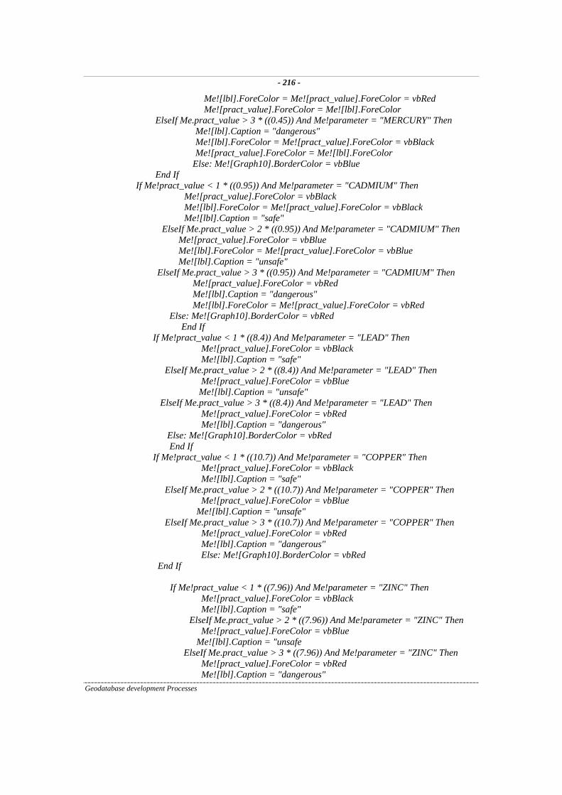
- 216 -


Me![lbl].ForeColor = Me![pract_value].ForeColor = vbRed Me![pract_value].ForeColor = Me![lbl].ForeColor

ElseIf Me.pract_value > 3 * ((0.45)) And Me!parameter = "MERCURY" Then Me![lbl].Caption = "dangerous" Me![lbl].ForeColor = Me![pract_value].ForeColor = vbBlack Me![pract_value].ForeColor = Me![lbl].ForeColor

Else: Me![Graph10].BorderColor = vbBlue End If If Me!pract_value < 1 * ((0.95)) And Me!parameter = "CADMIUM" Then

Me![pract_value].ForeColor = vbBlack Me![lbl].ForeColor = Me![pract_value].ForeColor = vbBlack Me![lbl].Caption = "safe"

ElseIf Me.pract_value > 2 * ((0.95)) And Me!parameter = "CADMIUM" Then Me![pract_value].ForeColor = vbBlue Me![lbl].ForeColor = Me![pract_value].ForeColor = vbBlue Me![lbl].Caption = "unsafe"

ElseIf Me.pract_value > 3 * ((0.95)) And Me!parameter = "CADMIUM" Then Me![pract_value].ForeColor = vbRed Me![lbl].Caption = "dangerous" Me![lbl].ForeColor = Me![pract_value].ForeColor = vbRed

Else: Me![Graph10].BorderColor = vbRed End If If Me!pract_value < 1 * ((8.4)) And Me!parameter = "LEAD" Then

Me![pract_value].ForeColor = vbBlack Me![lbl].Caption = "safe"

ElseIf Me.pract_value > 2 * ((8.4)) And Me!parameter = "LEAD" Then Me![pract_value].ForeColor = vbBlue Me![lbl].Caption = "unsafe"

ElseIf Me.pract_value > 3 * ((8.4)) And Me!parameter = "LEAD" Then Me![pract_value].ForeColor = vbRed Me![lbl].Caption = "dangerous"

Else: Me![Graph10].BorderColor = vbRed End If If Me!pract_value < 1 * ((10.7)) And Me!parameter = "COPPER" Then


ElseIf Me.pract_value > 2 * ((10.7)) And Me!parameter = "COPPER" Then Me![pract_value].ForeColor = vbBlue Me![lbl].Caption = "unsafe"

ElseIf Me.pract_value > 3 * ((10.7)) And Me!parameter = "COPPER" Then Me![pract_value].ForeColor = vbRed Me![lbl].Caption = "dangerous" Else: Me![Graph10].BorderColor = vbRed

End If

If Me!pract_value < 1 * ((7.96)) And Me!parameter = "ZINC" Then Me![pract_value].ForeColor = vbBlack Me![lbl].Caption = "safe"

ElseIf Me.pract_value > 2 * ((7.96)) And Me!parameter = "ZINC" Then Me![pract_value].ForeColor = vbBlue Me![lbl].Caption = "unsafe

ElseIf Me.pract_value > 3 * ((7.96)) And Me!parameter = "ZINC" Then Me![pract_value].ForeColor = vbRed Me![lbl].Caption = "dangerous"

- 217 -


Else: Me![Graph10].BorderColor = vbRed End If

If Me!pract_value < 1 * ((8.7)) And Me!parameter = "CHROMIUM" Then


ElseIf Me.pract_value > 2 * ((8.7)) And Me!parameter = "CHROMIUM" Then Me![pract_value].ForeColor = vbBlue Me![lbl].Caption = "unsafe"

ElseIf Me.pract_value > 3 * ((8.7)) And Me!parameter = "CHROMIUM" Then Me![pract_value].ForeColor = vbRed Me![lbl].Caption = "dangerous" Else: Me![Graph10].BorderColor = vbRed

End If On Error GoTo Err_Command116_Click

DoCmd.GoToRecord , , acNext Exit_Command116_Click:

Exit Sub

Err_Command116_Click: MsgBox Err.Description

Resume Exit_Command116_Click DoCmd.DoMenuItem acFormBar, acEditMenu, acUndo, , acMenuVer70

End Sub Row source

Transform Max(Subquery1.Pract_Value) As Maxofpract_Value Select Subquery1.Parameterfrom Subquery1 Where (((Subquery1.Discipline_Name)="Heavy_Metal")) Group By Subquery1.Parameter Pivot Subquery1.Station; Link Child Field = Station Link Parent Field = Station Obj.Name: Graph 10 Time Interval : 3000 Has A Module : True

- 218 -

References

[ 1 ] Kennet, J. P., 1982. Marine Geology. Prentice-Hall, Inc., Englewood Cliffs, N.J, 813 P.

[ 2 ] Shi, H. et al., 2001. The Status and Interconnections of Selected Environmental Issues of the Global Coastal

Zones: Problems Of Increasing Vulnerability. In: The Proceeding of the Coast GIS 01, Managing The

Interfaces, Halifax, and (Canada). 18-20 June 2001.

Progress and Problems in Preventing Pointless Pollution, Runoff Report Release. [ 3 ]

URL: http://www.coastalliance.org/press/pppress.htm, 1999.

[4 ] Massive Iceberg Peels Off from Antarctic Ice Shelf, (National Oceanic and Atmospheric Administration

satellite Image (NOAA). URL: http://uwamrc.ssec.wisc.edu/amrc/iceberg.html, March 21, 2000.

[ 5 ] Gilman, J. et al., 2001. Coastal GIS: An integrated system for coastal management. In: Proceedings of the

Coast GIS 01, Managing The Interfaces conference, In: The Proceeding of the Coast GIS 01, Managing The

Interfaces, Halifax, (Canada). 18-20 June 2001.

Training Modules on the Application of Geographic Information System (GIS) for the online Governances

and Access, Public Domain Information.

[ 6 ]

URL: http://ioc.unesco.org/oceanteacher/resourcekit/Module2/GIS/Module, UNESCO, 1999.

[ 7 ] What in the world is a 'GIS'? URL: http://www.census.gov/geo/www/faq-index.html.

[ 8 ] Wright, D., J. 1999. Down to the Sea in Ships: The Emergence of Marine Environment GIS. Marine and

coastal geographic information systems, Taylor and Francis.

[ 9 ] Tomlin, C. D., 1990. Geographic information systems and cartographic modeling Prentice-Hall, Inc

Englewood cliffs, N.J., 249 p.

[10] Components of GIS: http://www.njgin.co.somerset.nj.us/information/components.html#.

[11] Bentley (ed.), 1995. MicroStation geographic User’s Guide, Bentley Systems, Incorporated, Pennsylvanian

[12] Bentley (ed.), 1995. MicroStation 95, MicroStation Basic Guide. Bentley Systems, Incorporated,

Pennsylvania.

[13] Ghebre Egziabeher, T., Van Biesen, L., Yamba P., Cisneros. Z., 2000: The Construction and Implementation

of a Marine Environment Geographic Information System (GIS). In: The 6th proceedings of the 6th EC-GI &

GIS Workshop, Lyon (France), and 28-30 June 2000.

[14] Twilley, R. R., Gottfried, R.R., Rivera-Monroy, V. H., Zhang Wanqiao, Armijos, M. M., Bodero, Alcjandro,

1998. An approach and preliminary model of integrating ecological and economic constraints of

environmental quality in the Guayas River estuary, Ecuador. Environmental Science and Policy 1(1998) 271-

288.

[15] Zimmerman, R., Minello, T. J., 1986. Recruitment and distribution of post larval and early juvenile penaed

shrimp in a large mangrove estuary in the Gulf of Guayaquil during the 1985. In: Olsen, S., Arriaga. L (eds).

Establishing a sustainable shrimp Mari culture industry in Ecuador.

[16] Nunez, A., 1983, Conocimento Estratigrafico, Sedimentologic Y Tectonics de la Region Oriental de la

Peninsula de Santa Elena Y parte sur de la cuenca del Guayas (Ecuador) en base A17. In: Tercer congers

Ecuatoriano de Ingeneiros Geologos de minas Y Petrolleos p 1-31.

[17] Van Biesen, L., Cisneros. Z., Yamba P., Ghebre Egziabeher T., and Peirlnckx, L). Tackx, M., Tores, F.,

Roose, P., Gomez, h., Wartel, S., and Vincx, M., 1998. Development of a multi-disciplinary geographical

information system (GIS) of the Marine Environment in view of the monitoring and modeling of the Guayas

estuary and the Esterio Salado (Ecuador. In: The Proceeding of the oceans ’98 conference, Nice 28 sept-1 Oct

1998, and p.1168-1172.

http://www.coastalliance.org/press/pppress.htm

http://www.nsf.gov/od/lpa/news/press/00/pr0012.htm

http://uwamrc.ssec.wisc.edu/amrc/iceberg.html

http://uwamrc.ssec.wisc.edu/amrc/iceberg.html

http://ioc.unesco.org/oceanteacher/resourcekit/Module2/GIS/Module

- 219 -

[18] Bentley (ed.), 1996. MicroStation95 User’s Guide, Bentley Systems Incorporated, Pennsylvanian, USA.

[19] Bentley (ed.), 1996. MicroStation Terra Modeler. Bentley Systems Incorporated, Pennsylvania, USA.

[20] Intergraph (ed.), 1997. Modular Geographic Information System (MGE), Intergraph Corporation, USA.

[21] ESRI (ed.), 1996. ArcView GIS, The Geographic Information System for everyone, Environmental Research

Institute, Inc. N.Y, Redlands CA, USA.

[22] Bentley (ed.), 1997. Micro Station Geocoordinator. Bentley (Mizar) Systems, Incorporated, Pennsylvania.

[23] Date, C.J., 1995. An Introduction to Database Systems, 6th ed. Addison Wesley, 839p.

[24] ESRI, 1994. Arc/Info data management, concepts, data models, database design, and storage, N.Y, Redlands

CA., USA, 270P.

[25] Walker, R. ed (1993). AGI Standards Committee GIS Dictionary. In: Association for Geographic Information

2001, URL: http:// www.geo.ed.ac.uk/agidict/welcome.html.

[26] Jones, C. B., 1997. Geographic Information Systems and Computer Cartography, Addison Wesley 319p

[27] Longley P A, Maguire D J, Godchild M F, and Rhind D W (eds), 1991. Geographic Information Systems and

Science. Principles and applications, Longman.

[28] Stevens, A., (1992.) C++ Database Development, MIS: Press, 319P. N.Y., USA.

[29] Date, C.J., 1995. An Introduction to Database Systems, 6th ed. Addison Wesley, 839p.

[30] MapInfo (ed.), 2001. MapInfo professional Version 6.5. 1985-2000, MapInfo Corporation.

[31] Intergraph (ed), 1994. Modular GIS Environment. Intergraph Corporation, Huntsville, Alabama.

[32] Map OverView :-Peter H.Dana,http://www.colorado.edu/geography/gcraft/notes/mapproj/mapproj_f.html,

1995.

[33] Winteraecken, J.J.V.R., 1990. The NIAM Information Analysis Method: theory and practice, Kluwer

Academic pub. 469p.

[34] Simpson, A., et al, 1997. Mastering Access 97, fourth ed., SYBX inc., Marina Village Prkways, Alamada CA

–94501.USA.

[35] Smith. L Curtis and Amundsen M.M., (2000). Database programming with visual basic 6 Macmillan

Computer Publishing, Indianapolis, Indiana, USA. 855 P.

[36] MapInfo (ed.), 2002. MapBasic Development Environment Reference Guide, Version 7.0 1992-2002

MapInfo Corporation.

[37] MapInfo (ed.), 2001. MapInfo professional Version 7.0. 1985-2001, MapInfo Corporation.

[38] K. Van Hemelrijck, Y. Yan, P. Boets, L. Van Biesen, M. Persoons, A PC-Based Navigational GIS for Marine

Surveys, Proceedings of the Second Thematic Conference Remote Sensing for Marine and Coastal

Environments, (New Orleans, Louisiana, USA, 31 Jan - 2 Feb 1994), pp II-3-II-11.

[39] Oracle Corp, 1995. Oracle 7 server SQL language reference manual. Oracle Corporation Redwood City, Cal.

[40] Dictionary Of Abbreviations And Acronyms In Geographic Information Systems, Cartography, and Remote

Sensing. URL:- http://www.lib.berkeley.edu/EART/abbrev.html

[41] Mennecke, B.E., 1997. Understanding the role of geographic information Technology in Business:

Applications and research direction: In Journal of geographic information system and decision analysis, vol.1,

no1, pp. 44-68.

[42] Flood Impacts, Europe under water, URL: http://news.bbc.co.uk/2/hi/europe/2201763.htm, 2002.

http://www.terrainmap.conv/

http://news.bbc.co.uk/2/hi/europe/2201763.stm%5B

- 220 -

[43] Van Biesen, L. and Patrice Yamba P., 2002. Application of GIS for the Monitoring, Exploitation and

Sustainable Environmental Management of Marine Ecosystems. In: Tutorial Course for Young Acousticians

from European Countries, Lecture Notes, Edited by Z. Lubniewski and A. Stepnowski, ISBN 83-907591-4-4,

Gdansk, 2002, pp. 1938.

[44] Van Biesen, L., Patrice, T.K., Ghebre Egziabeber, T., and Zobeida C., 1999. "Monitoring and use of GIS for

sustainable environmental management". In: The Proceedings of the 3rd Biennial Conference MSA 99,

Measurement for a Sustainable Future, Sydney, Australia, 2224 September 1999, pp. 273277.

[45] Ghebre Egziabeher T., Van Biesen, L., Yamba P., 2001. "Integration and Implementation of a

multidisciplinary Coastal zone Geographic Information System (GIS)". : In: The Proceeding of the Coast GIS

01, Managing The Interfaces, Halifax, (Canada). 18-20 June 2001.

[46] Van Biesen, L., Cisneros Z, Ghebre Egziabeher T., 2003. On the application of the power of GIS to

environmental measurements for the monitoring, exploitation and sustainable environment of marine

ecosystems. In: XVII IMEKO world Congress, metrology in the 3rd millennium, Dubrovnik, Croatia.

[47] Van Biesen, L., Peirlinckx, L., Cisneros, Z., and Yamba, P. “Impact of Measurement Science in Sustainable

Management". In: the Proceedings of the IMEKO XIV World Congress, Tampere, Finland, June 1-6, 1997,

Vol. XA, pp 97-102.

[48] Rozakis S., Kallivrousisis L., Soldats Peter G., and Nicolaou I., 2001. Multiple Criteria Analysis of Bio-

Energy Project: Evaluation of Bio-Electricity production in Farsala Plain, Greece. Journal of Geographic

Information and decision analysis 2001, Vol. 5, No.1, pp.49-64.

[49] Vitalis K., Monalidiadis O., 2002. A two-level Multicritrea DSS for Landfill Site Selection using GIS: Case

study in Western Macedonia, Greece. Journal of Geographic Information and decision analysis 2002, Vol. 6,

No.1, pp.49-56.

[50] Marine protection, Research and Sanctuaries act and its Protection Regulations,URL:

http://www.coastalliance.org/mud/ch3.pdf, 1999.

Ecuador’s Coast, Complete online guide to Ecuador and the Galapagos Islands, URL: [51]

http://www.ecuadorexplorer.com/html/coast.html, 1997-2003.

[52] Rihnd, D.W., Mounsey, H., 1989. GIS/LIS in Britain in 1988. In: Shand P.J., Moore R.V. (eds.). The

association of geographic information Yearbook 1989.Taylor & Francis, London.

[53] Henderson Sellers A. & Robinson P.J., (1989). Contemporary Climatology. Longman Scientific and

Technical. Longman group UK, Longman House, Burnt Mill, Harlow, ESSEX cm20 2JE, England. 439p.

[54] Burrough, P.A., 1986. Principles of Geographic Information Systems for Land Resources Assessment.

Oxford: London.

[55] Bonham-Carter, G.F., 1994. Geographic Information Systems for Geoscientists: Modeling with GIS. In D.F.

Merrian, Series Editor: Computer Methods in the Geosciences. Vol.13, Pergamon, 398 pp, 1994.

[56] Ghebre Egziabeher, T., 1995. The Design and Development of a GeoDatabase Application in Geo-data

Process, Master degree Computer Science thesis, Vrije Universiteit Brussel, Department of computer science

(Informatics) 64p.

[57] Emani, S., Smuel, J., Clarck. E. R., Dow. K. G., Kasperson, J. X., Ksaperson, .R. E, Mouse. S and Schwarz.,

H., E., 1993. “Assessing Vulnerability extreme storm events and sea-level rise using Geographic Information

System (GIS)”. In: Proceedings GIS/LIS’93 Annual conference and exposition, Minneapolis, Minnesota,

November 2-4, 1993, .Vol. 1, pp 201- 218.

http://www.coastalliance.org/mud/ch3.pdf

http://www.ecuadorexplorer.com/HTML/COAST.HTML

http://www.ecuadorexplorer.com/html/coast.html

- 221 -

[58] Van Biesen, L., Yamba P., Ghebre Egziabeher T., S.Vanderplas and F. Louge, 1999. ”Integrating GIS in

Sediment Identification For GeoTechnics by Marine Acoustics. In: Proceedings of the 5th EG-GIS Workshop,

Stresa, (Italy), and 28-30 June 1999.

[59] Mezei L. M., 1992. Practical Laboratory Information Management for scientists & Engineers. Prentice- Hall,

Englewood Cliffs, New Jersey, 293P.

[60] Cronin, D.J., 1990. Mastering Oracle, Featuring Oracle’s SQL TM standard, Hayden Book Macmillan

Computer book publishing Division 542p.

[61] Humboldt Current Galapagos On line, UTR:

ttp://www.galapagosonline.com/Galapagos_Natural_History/Oceanography/Humboldt_Current.htm.

[62] Roman S., 1997. Access Database Design n & Programming, first ed. O’Reilly &Associates Inc, 251p.

[63] Longley D J., Goodchild M F., Rind D W., Maguire D J. (eds). 1999, Geographic Information Systems and

Science. John Wiley & Sons, Ltd, P184-203.

[64] GIS Technology and Spatial Analysis in Coastal Zone Management. URL :-

http://www.sustdev.org/journals/others/iczm/03.171.pdf

[65] Longley D J., Goodchild M F., Rind D W., Maguire D J. (eds). 1999, Geographic Information Systems and

Science. John Wiley & Sons, Ltd, P184-203.

[66] Snyder, D.J. (1987) Map projection-A working Manual. United States Geological Survey Professional Paper

1395, United states Government Printing Office.

[67] GIS Development: URL: http://www.gisdevelopment.net/tutorials/tuman006.htm

[68] Geographic Objects with Indeterminate Boundaries, P.A.Burrough and A.U.Frank (eds) Tailor and francis,

London, pp.171-187 (chapter 1)

[69] Worboys M.M., 1995, GIS- A computing perspective., Tailor and Francis

[70] Bruce, A. R., 2002. Developing GIS Solutions with MapObjects and Visual Basic, OnWord Press, 315p

[71] Visio Professional 2002, a working help on line manual

[72] Date, C.J. (1990) An Introduction to Database Systems. Vol. 1. (5th ed). Addison-Wesley

[73] Date, C. J. (1985) An introduction to database systems, Vol. II. Addison-Wesley

[74] Jung. D, Boutquin P.,Conley J.D., Edahl L..,Mauer L..,Purdum j., (1999). Visual Basic 6 Super Bible.

Macmillan Computer Publishing, Indianapolis, Indiana, USA. 855 P.

[75] The database Models :- (http:// unixspace.com/CONTEXT/DATABASE.html)

[76] SQL3 Object Model : - (http://WWW.OBJ.COM/X3H7/SQL3.HTM)

[77] ((Mat96) Nelson Mattos, “ An overview of SQL3 standard”, database technology institute, BM Santa Teressa

Lab., San Jose, CA, July 1996, Fttp://specckel.ncsl.nist.gov/isowg3/db1/Basedocs/SQL3)

[78] Object-Relational Database Systems - The Road Ahead : by Ramakanth S. Devarakonda URL:-

http://www.acm.org/crossroads/xrds7-3/ordbms.html

[79] [http://www.opengis.org/]

[80] Witold Fraczek, ESRI Applications Prototype Lab; ArcUser

Magazinehttp://www.mentorsoftwareinc.com/CC/gistips/TIPS1098.HTM,

[81] http://www.esri.com/news/arcuser/0703/geoid1of3.html].

[82] [Inter-governmental Committee on surveying and mapping, 02/04/01:

http://www.icsm.gov.au/icsm/gda/wgs84fact.pdf]

[83] http://www.mentorsoftwareinc.com/CC/gistips/TIPS1098.HTM,

[84] [http://mapserver.gis.umn.edu/doc36/proj.html#PSAD50/%20UTM%20zone%2017S]

http://www.gisdevelopment.net/tutorials/tuman006.htm

http://www.obj.com/X3H7/SQL3.HTM

http://www.mentorsoftwareinc.com/CC/gistips/TIPS1098.HTM


http://www.esri.com/news/arcuser/0703/geoid1of3.html

http://www.icsm.gov.au/icsm/gda/wgs84fact.pdf

http://www.icsm.gov.au/icsm/gda/wgs84fact.pdf


http://mapserver.gis.umn.edu/doc36/proj.html#PSAD50/%20UTM%20zone%2017S

- 222 -

[85] [Nicholas, A. koncz. 2002, Temporal data construct for multidimensional transportation GIS applications.

http://www.sit.wisc.edu/~nakoncz/TRB02_2834_temporal.pdf

[86] Armstrong, M. P., 1988, Temporality in spatial databases. Proceedings: GIS/LIS'88, 2:880-889.

[87] Langran, G. and Chrisman, N, R., 1988, A framework for temporal GI. Cartographica, 25(3):1-14.

[88] Beller, A., Giblin, T., Le, K. V., Litz, S., Kittel, T., and Schimel, D., 1991, A temporal GIS prototype for

global change research. Proceedings: GIS/LIS'91, 2:752-765.

[89] [Jill McCoy and Kevin Johnston, 2001-2002, Using ArcGIS Spatial Analyst, ESRI N.Y, RedLands, CA92373-

8100, USA.

[90] Oracle Spatial & Oracle Locator: Location Features for Oracle Database :

http://otn.oracle.com/products/spatial/index.html

[91] Informix blades spatial: http://www-306.ibm.com/software//data/blade module/

[92] DB2 Spatial Extender: http://www-306.ibm.com/Softwar//data/ spatial

[93] What is the Relationship between CAD and GIS?, Geographic Information Systems Services Division.

http://www.dot.co.pima.az.us/gis/whatis/cad-gis.htm

[94] Measuring Currents: Research on Physical Sciences, Virginia Institute of Marine Sciences (vims),

(http://vims.edu/physical/researchCurrentMeasure.htmm , 2004

[95] Robert R, Twilley R, and Rivera V. 1997, The Utility of a Dynamic Model to Address Ecological-Economic

Interactions: Shrimp Ponds and Mangroves in the Guayas River Estuary, Ecuador .

http://136.142.158.105/LASA97/gottfried.pdf -1

[96] Twilley, R.R., M. Pozo, V.H. Garcia, V.H. Rivera-Monroy, R. Zambrano, and A. Bodero. 1997. Litter dynamics

in riverine mangrove forests in the Guayas River estuary, Ecuador. Oecologia 111:109-122.,

http://www.ucs.louisiana.edu/~rrt4630/ms44.pdf -1

[97] Tectonics and Seismicityhttp://books.nap.edu/books/039048/html/29.html and Strain Partitioning And Active

Faulting During Oblique Convergence, Northern Andes

[98] Gutscher A., Malavieille J., Lallemand S., and Collot Y. 1999. Tectonic segmentation of the North Andean

margin: impact of the Carnegie Ridge collision. Earth and Planetary Science Letters (EPSL) 168 (1999) 255–

270 -7

[99] Tides and Navigation : http://www.sailingissues.com/navcourse7.html [99] -7,

[100] Lunar Tides: Astronomy 161, Solar System: University of

Tenesee,http://csep10.physutk.edu/astr161/lect/time/tides.html

101] Dalrymple, R.S., Zaitlin, B.A. and Boyd, R., 1992, Estuary facies models: conceptual basis and stratigraphic

implications. Journal of sedimentary petrology, vol. No. 6, 1992, p 1130-1146 102

[102] Pritchard, D.W., 1967, what is an estuary? Physical viewpoint, Lauff, G.H., ed., Estuaries: American Association

for the advancement of Science. Pub 83, p3-5. 103

[103] Our restless tides, a brief description of the basic astronomical factors, which produce tides and tidal currents,

http://www.co.ops.nos.noaa.gov/restless6.html); and Estuarine Research Reserve: Estuaries Feature Series

http://www.harborside.com/~ssnerr/tides.htm

[104] Basic concepts in physical oceanographic: Oceanic circulation and tidal models,

http://www.oc.nps.navy.mil/nom/day1/partc.html

http://www.sit.wisc.edu/%7Enakoncz/TRB02_2834_temporal.pdf

http://www.sit.wisc.edu/%7Enakoncz/TRB02_2834_temporal.pdf

http://www-306.ibm.com/software//data/blade

http://www.dot.co.pima.az.us/gis/whatis/cad-gis.htm

http://vims.edu/physical/researchCurrentMeasure.htmm

http://www.ucs.louisiana.edu/%7Errt4630/ms44.pdf




http://www.lehigh.edu/%7Easm3/AT_IAV.html

http://www.lehigh.edu/%7Easm3/AT_IAV.html

- 223 -

[105] [105] Introduction to the Hydrosphere: Ocean tides http://www.Physicalgeography.net, 1999-2004

[106] Geodesy and Tides: Netherlands National Institute for Marine and Coastal Management. www.getij.nl

[107] The Universal Law of Gravitation (Sir Isaac Newton) http://csep10.phys.utk.edu/astr161/lect/index.html

[108] Lunar Tides: http://csep10.phys.utk.edu/astr161/lect/time/tides.html

[109] Online Journey through Astronomy: http://csep10.phys.utk.edu/centermassframe.html

[110] NOAA, national oceanic service, http:/www.nos.noaa.gov/ tidal predictions.html and 140.90.121.76/publications/table3.pdf

[111] Sumich, J.L.1996. An Introduction to Biology of Marine Life,6th ed. Dubuque, IA: Wm. C. Brown. pp. 30-35.

[112] Thurman, H.V. 1994. Introductory Oceanography, seventh edition. New York, NY: Macmillan. pp. 252-276

[113] [NOAA’s: National Ocean service, Tides and currents: http://ocean service.noaa.gov/140.90.121.76/publications/tidepredictions.html

http://ocean/

modeling, designing and developing a multidisciplinary

Documents