modeling consumer preferences and price …jmcauley/pdfs/ consumer preferences and price...

Modeling Consumer Preferences and Price Sensitivitiesfrom Large-Scale Grocery Shopping Transaction Logs

Mengting Wan∗, Di Wang†, Matt Goldman†, Matt Taddy†, Justin Rao†,Jie Liu†, Dimitrios Lymberopoulos†, Julian McAuley∗

∗University of California, San Diego, CA, USA, †Microsoft Corporation, WA, USA∗{m5wan, jmcauley}@ucsd.edu,

†{wangdi, mattgold, taddy, justin.rao, jie.liu, dlymper}@microsoft.com

ABSTRACTIn order to match shoppers with desired products and pro-vide personalized promotions, whether in online or offlineshopping worlds, it is critical to model both consumer pref-erences and price sensitivities simultaneously. Personalizedpreferences have been thoroughly studied in the field of rec-ommender systems, though price (and price sensitivity) hasreceived relatively little attention. At the same time, pricesensitivity has been richly explored in the area of economics,though typically not in the context of developing scalable,working systems to generate recommendations. In this study,we seek to bridge the gap between large-scale recommendersystems and established consumer theories from economics,and propose a nested feature-based matrix factorization fra-mework to model both preferences and price sensitivities.Quantitative and qualitative results indicate the proposedpersonalized, interpretable and scalable framework is capableof providing satisfying recommendations (on two datasets ofgrocery transactions) and can be applied to obtain economicinsights into consumer behavior.

KeywordsRecommender System; Consumer Behavior; Price Elastic-ity; Matrix Factorization

1. INTRODUCTIONModeling consumer preferences and price sensitivities at

scale is useful in both online and offline shopping worlds:Matching shoppers with the most desired products can helpimprove overall satisfaction, while providing appropriate pro-motions may lead to increased basket sizes (and revenue).Grocery shopping is one of the most frequent and regularshopping patterns in an individual or household’s day-to-dayactivities. As a result, incredible volumes of data includingtransaction logs, product meta-data, and consumer demo-graphics, can be collected from a number of offline (e.g. Wal-

c©2017 International World Wide Web Conference Committee (IW3C2),published under Creative Commons CC BY 4.0 License.WWW 2017, April 3–7, 2017, Perth, Australia.ACM 978-1-4503-4913-0/17/04.http://dx.doi.org/10.1145/3038912.3052568

.

Consumer Behavior Model

(preference & price sensitivity)

Transaction Logs (with Price!);Product info.;Demographics

etc.

Optimizer

Product Recommendation;

Personalized Promotion

1. Buy or not? 2. Which product? 3. How many?

Category Purchase Product Choice Purchase Quantity

Yes! Selected!

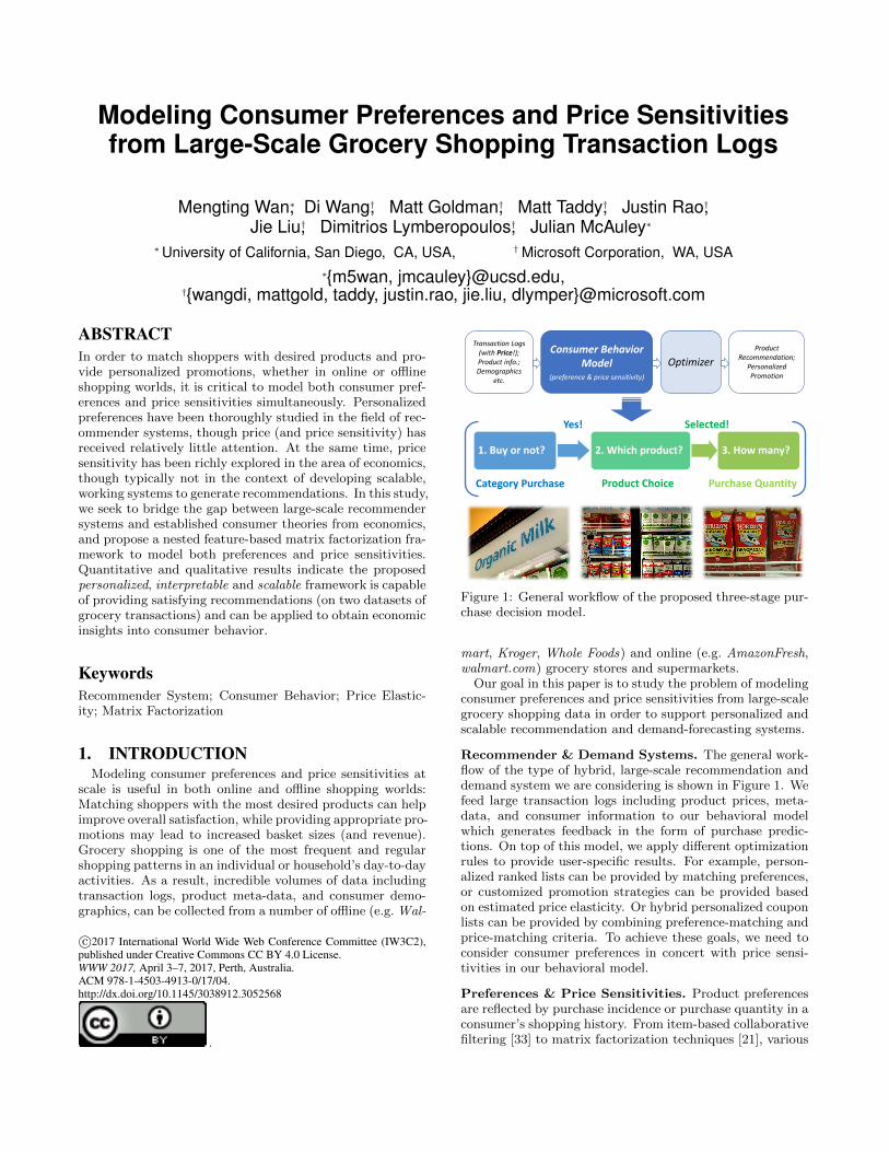
Figure 1: General workflow of the proposed three-stage pur-chase decision model.

mart, Kroger, Whole Foods) and online (e.g. AmazonFresh,walmart.com) grocery stores and supermarkets.

Our goal in this paper is to study the problem of modelingconsumer preferences and price sensitivities from large-scalegrocery shopping data in order to support personalized andscalable recommendation and demand-forecasting systems.

Recommender & Demand Systems. The general work-flow of the type of hybrid, large-scale recommendation anddemand system we are considering is shown in Figure 1. Wefeed large transaction logs including product prices, meta-data, and consumer information to our behavioral modelwhich generates feedback in the form of purchase predic-tions. On top of this model, we apply different optimizationrules to provide user-specific results. For example, person-alized ranked lists can be provided by matching preferences,or customized promotion strategies can be provided basedon estimated price elasticity. Or hybrid personalized couponlists can be provided by combining preference-matching andprice-matching criteria. To achieve these goals, we need toconsider consumer preferences in concert with price sensi-tivities in our behavioral model.

Preferences & Price Sensitivities. Product preferencesare reflected by purchase incidence or purchase quantity in aconsumer’s shopping history. From item-based collaborativefiltering [33] to matrix factorization techniques [21], various

methods for consumer preference matching have been devel-oped in the field of recommender systems. However, thereare few studies where price is considered as a factor, let alonethe relationship between preferences and price sensitivity.

On the other hand, price sensitivity has been richly stud-ied in the areas of economics and marketing, from classic de-mand systems [13] to customized promotion models [37,38].Demand systems are used to explore the relationship be-tween product prices and quantities sold. In this context,price sensitivity is measured by the ‘price elasticity’ valueobtained from a demand system, which is defined as the unitchange of purchase quantity (or probability) given a unitfluctuation in price [24]. In practice, elasticity-based con-sumer segments are considered and separate demand mod-els are constructed for different consumer segments. Suchsegments can be regarded as useful signals for retailers andmanufacturers to identify consumer groups to target. How-ever, there are two limitations in current demand systems:1) the data volumes involved are typically limited in termsof the number of products, categories and shopping trips1

and 2) classic demand models are not able to be updatedefficiently.

Therefore the major goal of this study is to constructan interpretable framework to model consumer preferencesand price sensitivities at scale, by connecting well-developedtechniques in recommender systems and well-established be-havioral economic theories.

Three-Stage Purchase Decision Model. Different frommodeling user preferences as a whole process, we follow thethree-stage framework from recent customized promotionstudies [37, 38]. We notice that in real-world grocery shop-ping scenarios, products can be categorized either based onan existing commodity hierarchy or by clustering their asso-ciated characteristics (e.g. text descriptions). Each categoryshould consist of some kind of products where consumers’purchase decisions share similar patterns. For example, onecategory might be ‘organic milk’ and two products in thiscategory could be ‘horizon organic whole milk’ and ‘organicvalley whole milk.’ As shown in Figure 1, we assume that fora given category, consumers’ purchase decisions can be de-composed into three stages: 1) category purchase incidence,2) product choice, and 3) purchase quantity. In a completepurchase decision-making process, stages are heterogeneousand consumers may behave quite differently across them.Given the fact that there are more than ten thousand dis-tinct products in a typical grocery store [1], this three-stagemodel is more efficient compared with a flat model withoutfine-grained product categorization [2, 14], since it can beconstructed in parallel across product categories and explic-itly interpreted across different purchase stages.

Specifically, we first consider whether a consumer willmake a purchase from a particular category in a certainshopping trip,2 which can be regarded as a binary predic-tion problem. If so, we model their purchase from this cate-gory following a multinomial distribution. Third, we deter-mine what quantity of the product will be purchased, whichleads to a numeric prediction problem. This combination

1Typical demand system studies [13, 18, 37, 38] usually in-volve only several products, categories and several hundredtransactions.2A ‘shopping trip’ in this study is represented as a (con-sumer, timestamp) pair.

of binary, categorical, and numeric prediction is quite dif-ferent from that used by traditional recommender systems,requiring new approaches to be developed. In particular,we develop a nested framework and extend state-of-the-artfeature-based matrix factorization models to include priceas a factor; this framework is embedded in the above pre-diction tasks with different link functions. We evaluate ourmodel on two real-world grocery shopping datasets whereour experiments reveal that the proposed framework is ca-pable of providing high-quality preference predictions andpersonalized price sensitivity estimates.

Contributions. Specifically, our contributions are as fol-lows:• We model consumer preferences and price sensitivities for

grocery shopping scenarios at scale, bridging a gap be-tween large-scale recommender systems and establishedeconomic theories.• We propose a nested feature-based matrix factorization

framework, which is flexible enough to include a range offeatures, to fit different prediction scenarios (for differentstages of purchase behavior), to be applied with scalablelearning algorithms (e.g. stochastic gradient descent) andcan be updated efficiently.• By applying matrix factorization techniques, separate con-

sumer segments no longer need to be extracted in advanceand personalized price elasticity can be obtained from themodel directly.• By applying the proposed framework, we can provide eco-

nomic insights from the results in our experiments. Theseinsights include: 1) price does not significantly affect cat-egory purchase decisions, suggesting that if the generalcategory of interest is not known, then ‘deal’ based pro-motions will be ineffective; 2) price is an important fac-tor in the product choice stage while there is wide vari-ance of price elasticities across categories, products andconsumers, which indicates that if the category of a con-sumer’s interest is known, it is effective to target appro-priate products and consumers in order to improve thefruitfulness of promotions.

2. RELATED WORKPreference matching has been richly studied in the area

of recommender systems, where two kinds of approaches ofinterest have been developed: 1) content-based approaches[23, 29], where explicit user profiles or item information areused as features, and 2) collaborative filtering approacheswhere preference predictions mainly rely on users’ previousbehavior [21,33]. By combining multiple techinques, hybridrecommender systems can be developed to handle a varietyof complex scenarios [8,17]. Matrix factorization techniqueshave been widely applied for recommender systems due totheir accuracy and scalability [6, 16, 21, 35]. Of particularinterest, feature-based matrix factorization techniques havebeen proposed [3,4,27,28,30] and efficient tools (e.g. SVD-feature, libFM) have been developed [9, 31]. Such ideashave been included in a recently proposed generalized lin-ear mixed model (GLMix) [39], which has been deployed inthe LinkedIn job recommender system with a scalable paral-lel block-wise coordinate descent algorithm. We build uponGLMix and adapt it to fit different prediction settings, suchas multi-class classification.

Demand systems and price sensitivity have been an ongo-ing focus of economists [2,13,14]. Three-stage purchase deci-sion decomposition (i.e., category purchase; product choice;purchase quantity), such as we consider here, has been ex-plored in several studies [5, 10, 18, 37, 38]. Customized pro-motion techniques have been recently proposed for offlineand online shopping behavior [12, 37, 38] where individualpurchase behavior is considered and optimal promotions arederived. However, these are not completely personalizeddemand systems and consumer segmentation is required be-forehand. In addition, none of these models is considered inthe context of large-scale predictive systems.

The idea of price sensitivity in recommender systems fore-commerce has been mentioned as a potential direction ina classic survey [34], though surprisingly we find that thisfactor has received relatively little attention. Optimiza-tion of online promotions in the context of recommenda-tion has been recently studied [19,20], where the reservationprice (i.e., the highest price a customer is willing to pay) isassumed as known information and a complete behavioralmodel is missing. The most related work is perhaps theprice-sensitive recommender system developed in [36]. Intheir study, however, price is discretized into different lev-els rather than evaluated numerically and personalization isnot thoroughly explored. Such a system thus struggles whenquantitatively estimating personalized price sensitivities andcannot effectively support customized promotion strategies.

3. BACKGROUNDIn this section, we introduce a generalized feature-based

matrix factorization approach, which can be adjusted andapplied in different purchase prediction stages. The basicnotation used in this paper is provided in Table 1.

3.1 A Unified Feature-Based Matrix Factor-ization Model

We extend the state-of-art GLMix approach [39] and con-sider a generalized Feature-Based Matrix Factorization(FMF) model:

link(Y (t)) = L(t) ≈ Φ(t)TΨ(t). (1)

Here Y (t) is the time-aware label matrix, where each ele-ment yi,u(t) indicates the label for an item i and a user u attimestamp t. yi,u(t) could be a binary label when predict-ing category purchase or product choice, or a numeric labelwhen predicting purchase quantity. By applying a link func-tion link(·) (e.g. the logit function, or logarithm function),we can transform the original label matrix into a numericmatrix L(t) and decompose L(t) as a product of Φ(t) andΨ(t). Here Φ(t) and Ψ(t) capture both explicit features andlatent factors from items and users. Specifically for each el-ement li,u(t) in L(t), we have

li,u(t) ≈ 〈φi(t),ψu(t)〉

=⟨w ,

global features︷︸︸︷g̃i,u(t)

⟩︸︷︷︸

global effect

+⟨item features︷︸︸︷φ̃

(o)i (t), ψ

(o)u

⟩+

⟨φ

(o)i ,

user feature︷︸︸︷ψ̃

(o)u (t)

⟩︸︷︷︸

observed item/user-specific effect

+⟨φ

(l)i ,ψ

(l)u

⟩︸︷︷︸

latent item-user interaction

,

(2)

where 〈·, ·〉 indicates the inner product. Here we decom-pose each prediction into three components: global effects,

Notation Description

i, u, t item, user, timestamp

(u, t) shopping trip associated with user u at time t

g̃i,u, w explicit global feature, global coefficient

φ̃(o)i (t), ψ̃

(o)u (t) explicit item feature, explicit user feature

φ(o)i , φ

(l)i item random coefficient, item latent factors

ψ(o)u , ψ

(l)u user random coefficient, item latent factors

µu(t) probability of user u selecting a category

ηi,u(t) conditional prob. of user u purchasing product i

q̂i,u(t) u’s conditional expected quantity of product i

β(·)i,u(t) coefficient associated with i’s price

e(cate)i,u (t) price elasticity in the category purchase stage

e(prod)ii,u (t) self price elasticity in the product choice stage

e(quant)i,u (t) price elasticity in the purchase quantity stage

Table 1: Notation.

observed item/user-specific effects and latent item-user in-teractions.

• Global effects. Here g̃i,u(t) includes a set of providedfeatures for (i, u, t) and w includes a set of global coeffi-cients which need to be estimated and should be consis-tent for ∀(i, u, t). Such features may include general tem-poral and spatial factors, such as day-of-week and storelocation.

• Observed item/user-specific effects. The next termcan be regarded as an analogy of the random coefficientmodel [22,25,36,39], which involves explicit features whose

coefficients are item- or user-dependent. Here φ̃(o)i (t) and

ψ̃(o)u (t) are explicit item- and user-related features (such

as item information, user demographics) while φ(o)u and

ψ(o)i are (latent) item- and user-dependent coefficients.

• Latent item-user interactions. The last component isdesigned to capture the remaining latent effects in terms

of low-rank user and item factors, where both φ(l)i ,ψ

(l)u

are latent parameters that need to be estimated.

Note that considering the identity link function link(x) = x,and discarding explicit features and timestamps, the aboveformulation extends typical matrix factorization formula-tions:

yi,u = b0 + bi + bu +⟨φ

(l)i ,ψ

(l)u

⟩. (3)

4. METHODOLOGYAs discussed, we assume that purchase decisions can be

predicted in three stages: category purchase incidence, prod-uct choice, and purchase quantity. In this section, we pro-pose a nested framework to holistically model the interde-pendence of these three stages, adopting the above FMFmodel as a building block in each stage.

4.1 A Nested Factorization FrameworkWe notice that in different categories, consumers’ pur-

chase patterns are different, which requires us to establish adistinct behavioral model for each category. Given a producti in category c, a consumer u, and a timestamp t, suppose

we have the following definitions:

Cu(t) : consumer u selects the category c at time t;

Bi,u(t) : consumer u purchases product i at t;

Qi,u(t) = q : consumer u’s purchase quantity of i at t is q.

Thus if we focus on the category c, a consumer’s preferencescan be represented by the joint probability of buying a cer-tain quantity of a particular product in category c, i.e.,

P (Qi,u(t) = q,Bi,u(t), Cu(t))

=P (Cu(t))︸︷︷︸category

preference

×P (Bi,u(t)|Cu(t))︸︷︷︸conditional

product preference

×P (Qi,u(t) = q|Bi,u(t), Cu(t))︸︷︷︸conditional quantity preference

.

(4)

This joint probability can be regarded as a product of threeconditional probabilities which represent the preferences inprevious purchase stages. By adopting different link func-tions in the previous FMF formulation, these three prefer-ences can be estimated by Logistic, Categorical, and Quant-ity-based FMF models.

• Category Purchase (L-FMF). For a given category c,we have the following logistic probability

µu(t) := PΘcate (Cu(t)) = σ(s(cate)u (t)), (5)

where σ(·) is the sigmoid function. Here s(cate)u (t) is a

category preference score, factorized using (2), where wehave only one general ‘item,’ i.e., the category c.

• Product Choice (C-FMF). Next we estimate the prob-ability of selecting a product within a category as a multi-nomial distribution via a softmax formulation:3

ηi,u(t) := PΘprod(Bi,u(t)|Cu(t)) =

exp(s(prod)i,u (t))∑

i′ exp(s(prod)i′,u (t))

. (6)

Similarly, we apply (2) to factorize the product preference

score s(prod)i,u (t).

• Purchase Quantity (Q-FMF) Purchase quantity canbe represented as a positive integer in {1, 2, . . .} and fol-lows a shifted Poisson distribution:

PΘquant (Qi,u(t) = q|Bi,u(t), Cu(t)) =zi,u(t)q−1 exp(−zi,u(t))

(q − 1)!,

(7)

where zi,u(t) = exp(s(quant)i,u (t)). Again we apply (2) to

factorize the quantity preference score s(quant)i,u (t). Notice

that the conditional expectation of purchase quantity canbe calculated as

q̂i,u(t) := EΘquant (Qi,u(t)|Bi,u(t), Cu(t)) = zi,u(t) + 1, (8)

which can be regarded as an estimate of Qi,u(t).

Finally, we let Θcate ,Θprod ,Θquant denote the sets of parame-ters involved in category purchase incidence, product choiceand purchase quantity prediction respectively.

3Note that given the fine-grained categories in our data(e.g. ‘organic milk’), the multinomial assumption can be jus-tified in most cases. If this were badly violated when userspurchase several different products in the same category, thisformulation is still helpful as providing the preference-basedproduct ranked list is sufficient in the personalized promo-tion and recommendation scenario.

4.2 InferenceSince the three purchase stages are heterogeneous, we as-

sume Θcate ,Θprod ,Θquant are separate parameter sets. Mod-els for each stage can then be inferred independently. Theproposed framework inherits the scalability of matrix factor-ization techniques, where efficient algorithms such as stochas-tic gradient descent can be applied [7]. We optimize allterms following the principle of maximum likelihood esti-mation (MLE). For a given category, we have the followinglikelihood functions for category purchase, product choiceand purchase quantity:

LLcate =∑u,t

[cu(t) log µu(t) + (1− cu(t)) log(1− µu(t))],

LLprod =∑i,u,t

bi,u(t) log ηi,u(t),

LLquant =∑i,u,t

[(qi,u(t)− 1) log zi,u(t)− zi,u(t)] + const ,

(9)

where const is a term independent of the parameters Θquant ,cu(t), bi,u(t) and qi,u(t) are corresponding labels for Cu(t),Bi,u(t) and Qi,u(t).4

Particularly for product choice, consumer purchase behav-ior is a kind of implicit feedback, in the sense that not pur-chasing a particular product does not necessarily indicatethat a consumer dislikes it. Thus rather than predictingif a product is selected via MLE, we can instead optimizea criterion that says purchased products are simply ‘morepreferred’ than non-purchased ones. This type of optimiza-tion criterion is captured by Bayesian Personalized Ranking(BPR) [32], a state-of-the-art technique that approximatelyoptimizes the area under the curve in terms of product rank-ings, i.e.,

AUC∗ =1

N

∑u,t

1

|P+u,t||P

−u,t|

∑i∈P+

u,t,i′∈P−u,t

δ(s(prod)i,u (t) > s

(prod)i′,u (t)),

(10)

where N is the total number of shopping trips for all con-sumers, P+

u,t is composed of the products selected by con-

sumer u at timestamp t and P−u,t includes (a random sam-ple of) products which were not selected. Here δ(·) is anindicator function (δ(x) = 1 if x is true; δ(x) = 0 other-

wise). δ(s(l)i,u(t) > s

(l)

i′,u(t)) = 1 indicates that the consumer

u prefers product i to product i′ (at timestamp t). In prac-tice, we maximize following objective function

LLBPR =∑i,u,t

bi,u(t)∑i′ 6=i

log pi>i′,u(t) (11)

where pi>i′,u(t) = σ(s(prod)i,u (t)− s(prod)

i′,u (t)).When optimizing the parameters above we adopt a simple

`2 regularization procedure in order to avoid overfitting.

4.3 Price Elasticity EstimationWe introduce the concept of ‘price elasticity’ to model

the product price sensitivity, which is a popular measurein economics and can be defined as the responsiveness of aproduct’s purchase quantity (or probability) to changes inits price (‘self elasticity’) or another product’s price (‘crosselasticity’) [11, 18]. Self elasticity values are usually neg-ative. Larger absolute values of elasticity indicate higher

4cu(t) = 1 indicates the incidence of Cu(t) and bi,u(t) = 1indicates the incidence of Bi,u(t)

price sensitivity, which means if the product price drops, itspurchase probability or purchase quantity will increase ac-cordingly. Since products within a category are often thesame kind of commodities (and likely to be substitutes),the cross elasticity values in the product choice stage areusually positive, which indicates that if the product pricedrops, purchase probabilities of other products within thesame category will decrease.

Suppose product prices are involved in previous FMFmodels by logarithmic transformations, and Pi(t) is definedas the price of product i at timestamp t. Due to the linearrepresentation of FMF, for a product i, we can represent

the previous preference scores s(cate)u (t), s

(prod)i,u (t), s

(quant)i,u (t)

as

s(cate)u (t) = r

(cate)u (t) + l

(cate)u +

∑i

β(cate)i,u (t) logPi(t),

s(prod)i,u (t) = r

(prod)i,u (t) + l

(prod)i,u + β

(prod)i,u (t) logPi(t),

s(quant)i,u (t) = r

(quant)i,u (t) + l

(quant)i,u + β

(quant)i,u (t) logPi(t).

(12)

where β(·)i,u(t) is the coefficient associated with the price of

product i, r(·)·,u(t) captures (temporal and spatial) contextual

information of the shopping trip (e.g. day-of-week, store lo-

cation) and l(·)·,u captures consumer u’s category loyalty or

product loyalty which is independent of the product’s priceand the environment of the shopping trip.5 Then we candefine the price elasticity of demand in different purchasestages.

• Category Purchase. For the probability of categorypurchase incidence and the price of product i in this cat-egory, we can define the elasticity as6

e(cate)i,u (t) :=

dµu(t)

µu(t)

/dPi(t)

Pi(t)≈ (1− µu(t))β

(cate)i,u (t). (13)

Based on (13), if we assume that β(cate)i,u (t) does not have

significant variations and e(cate)i,u (t) < 0, the absolute value

of e(cate)i,u (t) will decrease as the preference prediction µu(t)

increases.

• Product Choice. An advantage of our choice-basedmodel is that product competition within a category caneasily be modeled. That is, we can model the effect of aproduct’s price change not just to its own purchase prob-ability but other products’ purchase probabilities. To doso we define the self elasticity of i as

e(prod)ii,u (t) :=

dηi,u(t)

ηi,u(t)

/dPi(t)

Pi(t)≈ (1− ηi,u(t))β

(prod)i,u (t). (14)

As with (13) if β(prod)i,u (t) does not vary significantly and

e(prod)ii,u (t) < 0, the absolute value of e

(prod)ii,u (t) will decrease

as the associated preference prediction increases. For twoproducts i and i′, we have the cross elasticity (how a pricechange for i affects the sales of i′)

e(prod)ii′,u (t) :=

dηi′,u(t)

ηi′,u(t)

/dPi(t)

Pi(t)≈ −ηi,u(t)β

(prod)i,u (t). (15)

5Notice that r(·)·,u(t), l

(·)·,u and β

(·)i,u(t) can be composed of both

implicit parameters and explicit features.6This equation can be derived based on the fact thatd(log(x)) ≈ dx/x.

Notice that ηi,u(t)e(prod)ii,u (t) +

∑i′ 6=i ηi′,u(t)e

(prod)

ii′,u (t) = 0,which indicates that total choice shares must be conservedat the product selection level regardless of price fluctua-tions.

• Purchase Quantity. If we use the conditional expec-tation (8) as the estimation of the conditional purchasequantity, we have the following elasticity definition:

e(quant)i,u (t) :=

dq̂i,u(t)

q̂i,u(t)

/dPi(t)

Pi(t)≈ (1−

1

q̂i,u(t))β

(quant)i,u (t).

(16)

In this scenario, if the variance of β(quant)i,u (t) is limited and

e(quant)i,u (t) < 0, the absolute value of price elasticity will

increase as consumers’ preferences increase.

Notice that an advantage of the nested FMF framework isthat these three elasticities are additive. If we consider theprice elasticity for the whole shopping trip, since

EQi,u(t) =E(Qi,u(t)|Bi,u(t), Cu(t))P (Bi,u(t)|Cu(t))P (Cu(t))

=q̂i,u(t)ηi,u(t)µu(t)(17)

then this elasticity can be decomposed as

e∗i,u(t) =dEQi,u(t)

EQi,u(t)

/dPi(t)

Pi(t)= e

(cate)i,u (t)+e

(prod)ii,u (t)+e

(quant)i,u (t).

(18)

5. EXPERIMENTSWe evaluate the proposed nested feature-based matrix fac-

torization framework for consumer preference prediction andprice sensitivity estimation on two real-world grocery storetransaction datasets. For consumer preferences, we evaluatethe proposed FMF model’s ability to make satisfying pur-chase predictions in terms of category purchase incidence,product choice and purchase quantity estimation. In addi-tion, we provide analysis of the price elasticity estimationsand discuss the economic insights behind these observations.

5.1 DatasetsWe consider two real-world datasets of supermarket trans-

actions. MSR-Grocery is a new dataset of convenience storetransactions from a grocery store in the Seattle area; sincethis dataset is proprietary, we also evaluate our method onthe public Dunnhumby dataset to ensure the reproducibil-ity and extensibility of our results. Note that both datasetscontain instances of variability in the price of a given prod-uct due to promotions, making them an ideal platform tostudy the effect of price variability on consumer behavior.

• Dunnhumby. The first dataset is the The CompleteJourney dataset published by Dunnhumby.7 This datasetincludes transactions over two years from around two thou-sand households who are frequent shoppers at multiplestores of a retailer. Three-level category information isprovided in this dataset: department, commodity descrip-tion, and sub-commodity description. Here we regardthe most specific one as the category indicator. We fil-ter out small stores, infrequent shoppers, rare products,tiny categories, and finally obtain around 531 thousandproduct transactions8 from 98 thousand shopping trips

7https://www.dunnhumby.com/sourcefiles8Each product transaction is for a specific product in a shop-ping trip.

#producttransactions

#shoppingtrips

#users#tripsper user

Dunnhumby 531,201 98,020 799 123MSR-Grocery 152,021 53,075 1,228 43

#products #stores #categories#products

per category

Dunnhumby 4,247 108 104 42MSR-Grocery 1,929 1 55 35

Table 2: Basic dataset statistics.

by 799 consumers at 108 stores, across 4,247 productsand 104 categories. Consumer demographic information(household age, marital status, income, homeowner de-scription, household size, number of children, etc.) andproduct related information (retailer price, coupon infor-mation, manufacturer, brand, size, description, etc.) arealso included. We follow the dataset specification and cal-culate the actual product price based on the retailer priceand promotion information. By comparing the actualprice and retailer price, we find that 62% of the productsin transaction logs associated with these frequent shop-pers were sold on sale.

• MSR-Grocery . We collected eight months of transac-tions from a single (anonymous) convenience/grocery storein the Seattle area. After removing invalid transactions,infrequent shoppers, rare products, tiny categories, wekeep about 152 thousand product transactions from 53thousand distinct shopping trips by 1,228 frequent con-sumers across 1,929 popular products in 55 categories.Some product-related features (actual price, package size,size, description) are included, though we cannot obtainany consumer demographics due to the lack of a loyaltyprogram. Since the complete retailer price history is notavailable, we regard the maximum price in the transactionlogs as the retailer price and compare it with the actualprice. Ultimately around 50% of the products were soldon sale in this dataset.

Detailed statistics of above two datasets are included in Ta-ble 2.

5.2 Feature InstantiationRecall that in the general FMF representation in (2)

〈w, g̃i,u(t)〉︸︷︷︸global effect

+⟨φ

(o)i , ψ̃

(o)u (t)

⟩+

⟨φ̃

(o)i (t),ψ

(o)u

⟩︸︷︷︸

observed item/user-specific effects

+⟨φ

(l)i ,ψ

(l)u

⟩︸︷︷︸

latent interaction

both observed features and latent variables are involved. Inthis section, we will describe the general philosophy of fea-ture design in the context of the consumer behavior model,and the specific features used in each purchase stage for eachdataset.

• Category Purchase. For category purchase prediction,three global features (g̃i,u(t)) are considered: 1) consumeru’s previous category purchase frequency, which is usedto capture u’s category preference; 2) category purchasequantity in u’s last shopping trip, which is included tocapture u’s inventory information; 3) prices of productsin the given category c. Since popular products may havemore significant effects compared with unpopular prod-ucts from the same category, we transform product pricesinto log-scale, weighted by their cumulative sold quan-

tities. Since we have only one general ‘item’ (i.e., theselected category) at this stage, we only consider a simpleconsumer bias term and ignore latent item-user interac-tions.

• Product Choice. Similarly for a product i, we includethe following global features: 1) previous product pur-chase frequency by the consumer u; 2) current price of theproduct i (logPi(t)). Product biases and consumer biasesare included. logPi(t) is also considered in the item fea-

tures (φ̃(o)i (t)) such that each consumer and each product

has their own price-related coefficients. Latent item-userinteraction can be considered if provided product-relatedand consumer-related features are not sufficient.

• Purchase Quantity. For a product i, we consider theconsumer u’s previous average purchase quantity of theproduct and its current price as a global effect.

Besides the above mentioned features, additional featureconfigurations on the Dunnhumby dataset and the MSR-Grocery dataset can be found in Table 3.

5.3 Price History RecoveryIn real cases, the complete product price history may be

unavailable. Given the transaction logs, we can only observethe prices of those products sold at a certain timestamp.However, as we claimed in the previous section, prices ofunsold products ought to be included in the model as well,which requires us to attempt complete price history recov-ery. Specifically, we applied a simple ‘hot deck’ method [26]for imputing these missing prices, where the transactions aresorted by timestamps and the last observed price of the sameproduct is carried forward to the current missing price. Notethat this approach can be implemented efficiently but maygenerate biased values if people rarely buy products at theiroriginal price. Thus we claim that developing stronger ap-proaches to recover the complete price histories could be an-other important problem which can potentially be exploredas future research.

5.4 Baselines and Evaluation Methodology

Baselines. Consumers’ previous category purchase frequen-cies, product purchase frequencies and average purchase qua-ntities can be adopted as three simple baselines – cateFreq,prodFreq and avgQuant for category purchase, productchoice and purchase quantity predictions.

We also consider standard logistic regression (L-Reg) forcategory purchase where all the global features in Table 3are included. For product choice, matrix factorization asin (3) (MF-mle) is applied to fit the multi-class classifica-tion setting.9 L-Reg and MF-mle thus yield two learning-based recommendation benchmarks for category purchaseand product choice.

Finally, we apply two sets of FMF-based methods for allof these three prediction stages: 1) L-FMF-b, C-FMF-b-mle and Q-FMF-b are three FMF baselines where allfeatures in Table 3 except for product prices are included andthe MLE optimization criterion is applied; 2) L-FMF-p,C-FMF-p-mle and Q-FMF-p are three full FMF modelswhere product prices are added back. Comparing these twosets of baselines, the importance of product prices can be

9The dimension of φ(l)i , ψ

(l)u is set to 5.

Dataset global features (g̃i,u(t)) item features (ψ̃(o)u (t))

Dunnhumbycategory purchase freq., last purchase quant., day-of-week, storeID, household demographics,

prices of all productsintercept

MSR-Grocery category purchase freq., last purchase quant., day-of-week, prices of all products intercept

(a) Category Purchase

Dataset global features (g̃i,u(t)) item features (φ̃(o)i (t)) user features (ψ̃(o)

u (t))

Dunnhumbyproduct purchase freq., product price,

price*freq., price*day-of-week, price*storeIDintercept, product price,

product info. (brand, manufacturer, size description)intercept, product price,household demographics

MSR-Groceryproduct purchase freq., product price,

price*freq., price*day-of-weekintercept, product price,

product info. (package size, size description)intercept, product price

(b) Product Choice

Dataset global features (g̃i,u(t))

Dunnhumbyavg. purchase quant., day-of-week, storeID, product info., household demo., product price, price*(avg. quant.),

price*day-of-week, price*storeID, price*(product info.), price*(household demo.)

MSR-Grocery avg. purchase quant., day-of-week, product info., product price, price*quantity, price*day-of-week, price*product info.

(c) Purchase Quantity

Table 3: Specific features applied in FMF on the Dunnhumby and MSR-Grocery datasets. Notice that coefficients for theitem intercept and user intercept indicate consumer bias and product bias respectively.

evaluated. In addition to MLE, we adopt another methodC-FMF-p-bpr for product choice where the BPR criterion(11) is used to optimize the personalized product ranking(i.e., the AUC ∗) directly.

Evaluation Methodology. Note that the number of pur-chase incidences for each category is usually much smallerthan the total of those for the remaining categories in thecomplete transaction logs. Therefore we apply the area un-der the curve (AUC) metric to evaluate the performance ofcategory purchase prediction, which is suited to imbalancedbinary prediction tasks [15].

For product choice, in real-world recommender systems,one is often interested in providing satisfactory ranked listsinstead of simply predicting incidence. Thus we directlyadopt the AUC ∗ defined in (10), which measures if the se-lected product is preferred to those products that were notselected in each shopping trip.

Since purchase quantity estimation is a numeric predictiontask, we apply the mean absolute error (MAE) to evaluateperformance where

MAE =1

N∗

∑i,j,t

|q̂i,u(t)− qi,u(t)|, (19)

and N∗ indicates the total number of successful producttransactions in the given category. One advantage of thismeasure is that the MAE is more robust to outliers thanthe root mean squared error (RMSE).

5.5 ResultsWe chronologically partition shopping trips into 70/10/20

training/validation/test splits. Because of the number ofitem- and user-related parameters is very large, we set twodifferent coefficients on the `2 regularizers of the global pa-rameters (λ1) and the item-/user-related parameters (λ2).These coefficients are selected on the validation set.10 Allresults in this section are reported on the test data.

10λ1 is selected from {0.1, 0.5, 1, 5} and λ2 is selected from{1, 5, 10, 50}.

5.5.1 Preference PredictionWe evaluate the performance for preference prediction

based on the measures described in the previous section.

• Category Purchase. Results of category purchase pre-diction in terms of the AUC for binary classification areshown in Table 4a. Compared with the baseline cate-Freq, category prediction can be significantly improvedby incorporating additional features and consumer biases.However, we notice that price has little impact on perfor-mance, indicating that it may be difficult to drive con-sumers’ category purchase decisions by altering productprices.

• Product Choice. For product choice prediction, weevaluate the product-ranking AUC (i.e., AUC ∗ in (10)).Results across different categories are provided in Table4b. Compared with prodFreq and MF-mle, perfor-mance can be improved by incorporating more featuresand latent factors. We particularly notice the significanceof the price feature on the Dunnhumby dataset by com-paring the performance of C-FMF-b-mle and C-FMF-p-mle. Also in general, C-FMF-p-bpr reliably outper-forms other MLE-based methods by directly optimizingranking scores.

• Purchase Quantity. We include results for purchasequantity prediction in Table 4c. Again, performance canbe improved by including additional features in the Q-FMF model but product price features do not help sub-stantially.

5.5.2 Price Elasticity EstimationNext we consider price elasticity estimation. Table 5 shows

summary results (median, mean and standard deviation) ofthe elasticity distribution across all shopping trips in eachpurchase stage. Elasticity for product choice is calculatedfrom C-FMF-p-bpr.

Based on the results in Table 5, price elasticity for cate-gory purchase prediction is limited. This indicates that itis hard to drive consumers’ desire to purchase items from a

Dataset Dunnhumby MSR-Grocerymean s.e. mean s.e.

cateFreq 0.661 0.006 0.643 0.009L-Reg 0.722 0.006 0.657 0.009L-FMF-b 0.782 0.005 0.747 0.008L-FMF-p 0.783 0.005 0.746 0.007

(a) Category purchase prediction (AUC).


prodFreq 0.726 0.006 0.727 0.008MF-mle 0.723 0.006 0.641 0.006C-FMF-b-mle 0.824 0.005 0.802 0.007C-FMF-p-mle 0.830 0.005 0.802 0.007C-FMF-p-bpr 0.832 0.005 0.808 0.007

(b) Product choice (AUC*).


avgQuant 0.706 0.033 0.386 0.021Q-FMF-b 0.372 0.023 0.123 0.022Q-FMF-p 0.372 0.025 0.115 0.021

(c) Purchase quantity prediction (MAE).

Table 4: Mean and standard error of preference prediction results across different categories in different purchase stages onthe Dunnhumby and MSR-Grocery datasets.

Dunnhumby MSR-GroceryDataset median mean s.d. median mean s.d.

cate. purchase -0.001 -0.012 0.029 -0.025 -0.055 0.062product choice -0.798 -0.842 0.683 -0.117 -0.242 0.551purchase quant. -0.141 -0.196 0.213 -0.004 -0.024 0.067

Table 5: Summary of self price elasticity estimation.

particular category by a single product promotion (at leastfor grocery shopping). Compared with category and quan-tity prediction, product choice is the most price sensitivestage (in terms of elasticity) in the decision making pro-cess, while price still serves as an important, but less sig-nificant, feature for quantity prediction (especially on theDunnhumby dataset). We also notice that consumers in theDunnhumby dataset are more price-sensitive than those inthe MSR-Grocery dataset in the product choice and pur-chase quantity stages. One possible reason is that the MSR-Grocery dataset is collected from a convenience store, wherepeople usually have certain targets in mind and are less likelyto seek a large inventory of products. On the other hand, theDunnhumby dataset is composed of household-level shop-ping transactions where consumers may be more likely toredeem promotions and purchase more products.

In Table 6, we provide details of the eight most price-sensitive categories in each purchase stage. From Table 6b,we notice that consumers tend to select the most inexpen-sive products when shopping for meat (bacon, pork rolls,tuna), eggs, drinks (water, juice, coffee), cereal and snacks(potato chips, candy). In addition, from Table 6c we observethat consumers are more likely to stock products which haverelatively long shelf lives (e.g. frozen food, soft drinks) if ap-propriate promotions are offered. Some featured categories(categories with promotions and located in designated ar-eas) in the MSR-Grocery dataset appear in Table 6a andTable 6b, which indicates that a combination of promotionsand advertisements may help to affect consumers’ purchasedecisions.

6. CASE STUDY: BACONBesides showing the overall preference prediction perfor-

mance and the price elasticity distribution across the 104categories in the Dunnhumby and 55 categories in the MSR-Grocery dataset, we provide detailed explorations of themost price sensitive category from the Dunnhumby datasetin the product choice stage: ‘bacon (economy).’ A sum-mary of product prices in this category is included in Table7, where price variabilities can be observed for all productsexcept product 10. We also include the total quantity soldfor each product in Table 7, where we notice that productswith moderate prices are more popular than others.

p1

p2

p3

p4

p5

p6

p7

p8

p9

p10

p11

u1 u2 u3 u4 u5 u6 u7 u8 u9 u10

consumer

pro

duct

−0.5

−0.4

−0.3

−0.2

−0.1

elasticity


p1

p2

p3

p4

p5

p6

p7

p8

p9

p10

p11

u1 u2 u3 u4 u5 u6 u7 u8 u9 u10

consumer

pro

duct

−3.0

−2.5

−2.0

−1.5

elasticity

(b) Product Choice

p1

p2

p3

p4

p5

p6

p7

p8

p9

p10

p11

u1 u2 u3 u4 u5 u6 u7 u8 u9 u10

consumer

pro

duct

−0.5

−0.4

−0.3

−0.2

−0.1

0.0elasticity


Figure 2: Heatmaps of consumer-specific price elasticity indifferent purchase stages for the example category ‘bacon(economy).’ Darker blocks indicate higher price sensitivity.

Preference vs. Representative Features. We find thatthe estimated coefficient on ‘bacon (economy)’ for categoryfrequency in the category purchase stage is 0.28, which in-dicates that a consumer’s previous category purchase fre-quency is still positively related to the category preference.Also the estimated coefficient for last purchase quantity is−0.22, which means if consumers purchased a substantialvolume of economy bacon products in their previous shop-ping trips, they may avoid making the same category pur-chase in their current shopping trip. For the product choicestage and the purchase quantity stage, we find that the es-timated coefficients for product frequency and average pur-chase quantity are 0.28 and 0.20, which indicates these twofeatures are positively correlated with preferences as well.

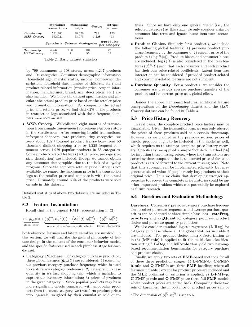
Personalized Product-Specific Price Sensitivity. Am-ong the 11 products in the example category ‘bacon (econ-omy)’ there are 448 consumers who have purchased prod-ucts in this category. We randomly select 10 consumers andcalculate their average price elasticity for each ‘bacon (econ-omy)’ product in terms of category purchase, product choiceand purchase quantity decisions. Heatmaps of the resultsare shown in Figure 2. We notice that within the ‘bacon(economy)’ category, different consumers and products mayhave significantly different price sensitivities in each of thethree stages, though the personalized elasticity is not obvi-ous in Figure 2a since the user-specific price coefficient is notconsidered in the first stage. By setting appropriate thresh-olds for price elasticity, we can easily uncover those pricesensitive consumer-product pairs in Figure 2 and customizepromotion strategies accordingly. In addition, we find thatin Figure 2a, consumers are more sensitive to the prices ofproducts 2–6 in the category purchase stage, which indeedare popular products as we observed in Table 7. This impliesthat while it is hard to increase the possibility of categorypurchase incidence, promotions on popular products will bemore effective than others in terms of category purchase.

Preference vs. Price Sensitivity. Recall we claimed thatif the variances of price-associated coefficients in (13), (14),(16) are limited, then consumers with high preference scoreswill be relatively insensitive to price changes as far as cat-

Dunnhumby MSR-Grocery

bacon (economy) -0.04 broth -0.19soft drinks (20/24pk) -0.04 spices -0.17beef (lean) -0.01 popcorn -0.15garbage compactor -0.01 energy drinks -0.15hot dogs -0.01 chocolate -0.14pork rolls -0.01 pizza -0.11salad -0.01 tortilla chips* -0.10baby diapers -0.01 protein bars -0.10



bacon (economy) -2.59 eggs -1.65milk (white) -1.96 coffee -1.18butter -1.84 chips -1.07cereal (family) -1.79 bottle water -1.06juice -1.78 tortilla chips* -0.98tuna -1.77 bottled dill -0.82cereal (kids) -1.67 fresh bread -0.80pork rolls -1.67 candy -0.80

(b) Product choice


mac & cheese -0.47 chocolate -0.12soft drink (12/15/18pk) -0.44 candy -0.06bacon (economy) -0.41 energy drinks -0.05hot dogs -0.41 mac & cheese -0.04milk (white) -0.34 sausage -0.04pork rolls -0.33 frozen fruit -0.04frozen dinner -0.32 spices -0.04facial tissue -0.32 soft drinks -0.04


Table 6: The eight most price sensitive categories regarding three different purchase stages on the Dunnhumby and MSR-Grocery datasets. Values are the median self-elasticities within each category. Categories marked with * are composed offeatured products at special locations of the store.

Product prod. 1 prod. 2 prod. 3 prod. 4 prod. 5 prod. 6 prod. 7 prod. 8 prod. 9 prod. 10 prod. 11

mean $1.95 $2.99 $2.88 $3.09 $3.02 $3.08 $3.38 $3.83 $3.90 $5.99 $5.66standard deviation $0.14 $0.72 $0.62 $0.67 $0.71 $0.77 $0.86 $0.66 $0.54 $0.00 $0.53

minimum $1.49 $2.00 $2.00 $2.00 $1.50 $2.50 $2.50 $0.99 $2.49 $5.99 $3.99maximum $1.99 $3.99 $3.99 $3.99 $3.99 $4.39 $4.39 $4.49 $4.99 $5.99 $5.99

# unique values 4 4 4 4 8 5 5 4 5 1 3

quantity sold 204 373 215 455 730 507 173 64 65 32 30

Table 7: Summary of product prices and sold quantities on ‘bacon (economy)’.

egory and product choice is concerned, but they tend tobe price sensitive with respect to purchase quantity. Againtaking ‘bacon (economy)’ as an example, in Figure 3 weshow the relationship between preferences and price sen-sitivities in different purchase stages. We notice that allelasticity values are negative, which is consistent with theintuition that purchase probability will increase if productprice drops. Here absolute price elasticity values are gener-ally negatively correlated with preferences in category pur-chase and product choice, but positively correlated withpurchase quantity, which indeed verifies our previous argu-ments about the relationship between preference and pricesensitivity. In Figure 3b, we notice that ‘low-preference’consumers have larger variations in price sensitivity than‘high-preference’ consumers. This is possibly because high-preference consumers’ preferences dominate purchase deci-sions (i.e., 1−ηi,u(t) is close to zero in (14)) and they tend topurchase a product no matter its price. On the other hand,if a product is not preferred by a consumer, this could beeither because the price is too high to trigger a purchase, orbecause the consumer simply dislikes the product. In Figure3c, we observe that those consumers with strong preferencesare not the most price-sensitive consumers. This observa-tion is consistent with the intuition that aggressive buyersare more likely to exhaust the potential of purchase quantitydue to budget limits so that it would be difficult to increasetheir purchase quantities by adjusting price.

7. CONCLUSIONS AND FUTURE WORKWe systematically studied the problem of modeling con-

sumer preferences and price sensitivities, and proposed anested feature-based matrix factorization framework to sup-port personalized and scalable recommendation and demandsystems. We verified that the proposed model is capableof providing high quality preference predictions and specificprice elasticity can be appropriately estimated for each shop-ping trip. By applying the proposed framework on two real-world datasets, we provided economic insights which maybenefit both data mining and economics communities. Par-

−0.6

−0.4

−0.2

0.0

0.0 0.1 0.2 0.3 0.4

category preference

pri

ce e

last

icit

y


−3

−2

−1

0

0.00 0.25 0.50 0.75

product preference

pri

ce e

last

icit

y

(b) Product Choice

−0.75

−0.50

−0.25

0.00

0.0 0.5 1.0 1.5 2.0

quantity preference

pri

ce e

last

icit

y


product prod. 1 prod. 2 prod. 3 prod. 4 prod. 5 prod. 6 prod. 7 prod. 8 prod. 9 prod. 10 prod. 11

Figure 3: Scatter plots between preference prediction andprice elasticity estimation in different purchase stages forthe example category ‘bacon (economy)’. Note that axeswithin each subfigure are scaled based on their own ranges.

ticularly, we noticed that price affects product choice buthas limited effects on category purchase or product quantity,which means coupons are primarily effective “within cate-gory”. Grocery shopping behavior is particularly exploredin this study but the nested multi-stage framework and therelationship between preference and price sensitivities canbe translated to other domains (e.g. clothes shopping, on-line advertising).

Price sensitivity in large-scale systems is an importantproblem and a number of possible topics can be exploredalong this trajectory. For example, temporally-aware mod-els could be developed to allow long-term purchase patternsto be carefully studied. Cross elasticity has been introducedbut not completely explored in this work; this could be stud-ied in detail in future work where not only product substi-tution but product complementarity could be modeled. Inaddition, since the straightforward imputation method weapplied to recover price history will be problematic if peoplerarely buy products at their original price, another possibledirection could be to develop more sophisticated approachesfor price history recovery by combining preference predictionand missing price inference. In the context of hybrid recom-mender and demand systems, we have so far only studiedconsumer behavior in this work, but the optimization strate-gies could be adapted to generate personalized coupons.

8. REFERENCES[1] Supermarket Facts. Food Marketing Institute,

Accessed Oct. 2016. http://www.fmi.org/research-resources/supermarket-facts.

[2] D. A. Ackerberg. Advertising, learning, and consumerchoice in experience good markets: an empiricalexamination. International Economic Review,44(3):1007–1040, 2003.

[3] D. Agarwal and B.-C. Chen. Regression-based latentfactor models. In SIGKDD, 2009.

[4] A. Ahmed, B. Kanagal, S. Pandey, V. Josifovski, L. G.Pueyo, and J. Yuan. Latent factor models withadditive and hierarchically-smoothed user preferences.In WSDM, 2013.

[5] N. Arora, G. M. Allenby, and J. L. Ginter. Ahierarchical bayes model of primary and secondarydemand. Marketing Science, 17(1):29–44, 1998.

[6] L. Baltrunas, B. Ludwig, and F. Ricci. Matrixfactorization techniques for context awarerecommendation. In RecSys, 2011.

[7] L. Bottou. Large-scale machine learning withstochastic gradient descent. In COMPSTAT, pages177–186, 2010.

[8] R. Burke. Hybrid recommender systems: Survey andexperiments. UMUAI, 12(4):331–370, 2002.

[9] T. Chen, W. Zhang, Q. Lu, K. Chen, Z. Zheng, andY. Yu. SVDFeature: a toolkit for feature-basedcollaborative filtering. JMLR, 13:3619–3622, 2012.

[10] P. K. Chintagunta. Investigating purchase incidence,brand choice and purchase quantity decisions ofhouseholds. Marketing Science, 12(2):184–208, 1993.

[11] L. G. Cooper and M. Nakanishi. Market-shareanalysis: Evaluating competitive marketingeffectiveness, volume 1. Springer Science & BusinessMedia, 1989.

[12] P. J. Danaher, M. S. Smith, K. Ranasinghe, and T. S.Danaher. Where, when, and how long: factors thatinfluence the redemption of mobile phone coupons.Journal of Marketing Research, 52(5):710–725, 2015.

[13] A. Deaton and J. Muellbauer. An almost idealdemand system. The American economic review,70(3):312–326, 1980.

[14] A. M. Degeratu, A. Rangaswamy, and J. Wu.Consumer choice behavior in online and traditionalsupermarkets: The effects of brand name, price, andother search attributes. International Journal ofresearch in Marketing, 17(1):55–78, 2000.

[15] T. Fawcett. An introduction to ROC analysis. Patternrecognition letters, 27(8):861–874, 2006.

[16] P. Forbes and M. Zhu. Content-boosted matrixfactorization for recommender systems: experimentswith recipe recommendation. In RecSys, 2011.

[17] A. Gunawardana and C. Meek. A unified approach tobuilding hybrid recommender systems. In RecSys,2009.

[18] S. Gupta. Impact of sales promotions on when, what,and how much to buy. Journal of Marketing research,pages 342–355, 1988.

[19] Y. Jiang and Y. Liu. Optimization of onlinepromotion: a profit-maximizing model integratingprice discount and product recommendation.

International Journal of Information Technology &Decision Making, 11(05):961–982, 2012.

[20] Y. Jiang, J. Shang, Y. Liu, and J. May. Redesigningpromotion strategy for e-commerce competitivenessthrough pricing and recommendation. InternationalJournal of Production Economics, 167:257–270, 2015.

[21] Y. Koren, R. Bell, C. Volinsky, et al. Matrixfactorization techniques for recommender systems.IEEE Computer, 42(8):30–37, 2009.

[22] N. T. Longford. Random coefficient models. InHandbook of statistical modeling for the social andbehavioral sciences, pages 519–570. Springer, 1995.

[23] P. Lops, M. De Gemmis, and G. Semeraro.Content-based recommender systems: State of the artand trends. In Recommender systems handbook, pages73–105. Springer, 2011.

[24] N. Mankiw. Principles of Microeconomics. EconomicsSeries. Cengage Learning, 2011.

[25] C. E. McCulloch and J. M. Neuhaus. Generalizedlinear mixed models. Wiley Online Library, 2001.

[26] F. J. Molnar, B. Hutton, and D. Fergusson. Doesanalysis using “last observation carried forward”introduce bias in dementia research? CanadianMedical Association Journal, 179(8):751–753, 2008.

[27] X. Ning and G. Karypis. Sparse linear methods withside information for top-n recommendations. InRecSys, 2012.

[28] S. Park, Y.-D. Kim, and S. Choi. Hierarchicalbayesian matrix factorization with side information. InIJCAI, 2013.

[29] M. J. Pazzani and D. Billsus. Content-basedrecommendation systems. In The Adaptive Web, pages325–341. Springer, 2007.

[30] I. Porteous, A. U. Asuncion, and M. Welling. Bayesianmatrix factorization with side information anddirichlet process mixtures. In AAAI, 2010.

[31] S. Rendle. Factorization machines with libfm. TIST,3(3):57, 2012.

[32] S. Rendle, C. Freudenthaler, Z. Gantner, andL. Schmidt-Thieme. BPR: Bayesian personalizedranking from implicit feedback. In UAI, 2009.

[33] B. Sarwar, G. Karypis, J. Konstan, and J. Riedl.Item-based collaborative filtering recommendationalgorithms. In WWW, 2001.

[34] J. B. Schafer, J. Konstan, and J. Riedl. Recommendersystems in e-commerce. In EC, 1999.

[35] A. P. Singh and G. J. Gordon. A unified view ofmatrix factorization models. In ECMLPKDD, 2008.

[36] P. Umberto. Developing a price-sensitive recommendersystem to improve accuracy and business performanceof ecommerce applications. International Journal ofElectronic Commerce Studies, 6(1):1, 2015.

[37] J. Zhang and L. Krishnamurthi. Customizingpromotions in online stores. Marketing Science,23(4):561–578, 2004.

[38] J. Zhang and M. Wedel. The effectiveness ofcustomized promotions in online and offline stores.Journal of Marketing Research, 46(2):190–206, 2009.

[39] X. Zhang, Y. Zhou, Y. Ma, B. Chen, L. Zhang, andD. Agarwal. Glmix: Generalized linear mixed modelsfor large-scale response prediction. In SIGKDD, 2016.

modeling consumer preferences and price …jmcauley/pdfs/ consumer preferences and price...

Documents