Louisiana State UniversityLSU Digital Commons

LSU Master's Theses Graduate School

2016

Modeling Churn and Annular Flow Regimes inVertical and Near-Vertical Pipes with Small andLarge DiametersErika Viana PaganLouisiana State University and Agricultural and Mechanical College, evpagan@gmail.com

Follow this and additional works at: https://digitalcommons.lsu.edu/gradschool_theses

Part of the Petroleum Engineering Commons

This Thesis is brought to you for free and open access by the Graduate School at LSU Digital Commons. It has been accepted for inclusion in LSUMaster's Theses by an authorized graduate school editor of LSU Digital Commons. For more information, please contact gradetd@lsu.edu.

Recommended CitationViana Pagan, Erika, "Modeling Churn and Annular Flow Regimes in Vertical and Near-Vertical Pipes with Small and Large Diameters"(2016). LSU Master's Theses. 1140.https://digitalcommons.lsu.edu/gradschool_theses/1140

MODELING CHURN AND ANNULAR FLOW REGIMES IN VERTICAL AND NEAR-VERTICAL PIPES WITH SMALL AND LARGE DIAMETERS

A Thesis

Submitted to the Graduate Faculty of the Louisiana State University and

Agricultural and Mechanical College in partial fulfillment of the

requirements for the degree of Master of Science in Petroleum Engineering

in

The Department of Petroleum Engineering

by Erika Viana Pagan

B.S., Universidade Federal do Ceará, 2011 August 2016

ii

Acknowledgements

I would like to thank Louisiana State University for funding this research. I sincerely

thank my supervisor Professor Paulo Waltrich for his mentoring, support, and patience

throughout the duration of this study. His guidance and support have been profoundly valuable to

me. I extend my gratitude to Professor Wesley Williams and Professor Seung Kam for helping

me on the development of this research and for all the helpful and indispensable assistance when

it was necessary.

Special thanks go to my husband Renato Coutinho for believing in my potential and for

having always encouraged me to face new challenges, and helping on my personal and

professional growth. I also acknowledge the support and care of my entire family, especially to

my mother Maria das Dores Viana Pagan and my grandmother Elza Coelho, my brother Filipe

Pagan, and my father Jose Carlos Pagan who stayed in my mother country, but have always been

tracking my path, always hoping for new and great achievements in my life.

I also would like to express my gratitude to Pedro Sousa for sharing with me some of his

knowledge and experience. Very special thanks to Matheus Pareto, Bruno Xavier, and Felipe

Maciel for assistance getting some experimental data for this research and also for the assistance

on implementing the model and running some of the simulations.

I am thankful to the faculty and staff of the Petroleum Engineering department who were

essential to my learning process. I am also grateful to all the friends I conquered during my

Master studies from the LSU Petroleum Engineering Department as well as from outside of

school for helping this experience to be even more enjoyable.

iii

Table of Contents

Acknowledgements ......................................................................................................................... ii 

List of Tables ...................................................................................................................................v 

List of Figures ................................................................................................................................ vi 

Abstract ........................................................................................................................................ viii 

1.  Introduction ................................................................................................................................ 1  Flow Regimes .................................................................................................................... 2 1.1 Two-Phase Flow Modeling in Small and Large Diameter Pipes ...................................... 5 1.2 Objectives .......................................................................................................................... 6 1.3 Thesis Outline .................................................................................................................... 7 1.4

2. Literature Review ....................................................................................................................... 9  Two-Phase Flow Modeling ............................................................................................... 9 2.1

2.1.1  Liquid Holdup ............................................................................................................ 9 2.1.2  Pressure Gradient ..................................................................................................... 10 

2.1.2.1 Superficial Velocities ......................................................................................... 12 2.1.3  Annular Flow ........................................................................................................... 13 2.1.4  Churn Flow .............................................................................................................. 13 2.1.5  Correlations Available in the Literature .................................................................. 15 

2.1.5.1 Duns and Ros (1963) Correlation ...................................................................... 16 2.1.5.2 Gray (1974) Correlation ..................................................................................... 16 2.1.5.3 Ansari et al. (1994) Correlation ......................................................................... 17 2.1.5.4 OLGA (2000) Correlation .................................................................................. 17 

 Liquid Loading ................................................................................................................ 18 2.22.2.1  Turner et al. (1969) Droplet Model .......................................................................... 18 2.2.2  Minimum Pressure Point and Nodal Analysis ......................................................... 19 2.2.3  Coupled Reservoir/Wellbore Modeling ................................................................... 20 

3. Models Description .................................................................................................................. 23  Churn and Annular Flow Modeling ................................................................................ 23 3.1

3.1.1  Momentum Equations .............................................................................................. 23 3.1.2  Wall and Interfacial Shear Stress ............................................................................. 25 3.1.3  The Churn to Annular Flow Transition ................................................................... 28 3.1.4  The Slug/Bubble to Churn Flow Transition ............................................................ 28 3.1.5  Main Contributions of Proposed Model .................................................................. 30  Liquid Loading Initiation Model ..................................................................................... 31 3.2

3.2.1  Reservoir Inflow Performance Model (IPR) ............................................................ 34 3.2.2  Tubing Performance Relationship (TPR) ................................................................ 34 

4. Model Validation, Results and Discussions ............................................................................. 38  Churn and Annular Flow Modeling Validation Results .................................................. 38 4.1

4.1.1  Comparison with Laboratorial Data......................................................................... 39 

iv

4.1.2  Comparison with Field Data .................................................................................... 46  Liquid Loading Modeling Validation and Result Discussions ....................................... 51 4.2

4.2.1  Testing the Concept of Minimum Pressure Point and Nodal Analysis (Lea et al., 2003) with Field Data of Veeken et al. (2010) .................................................................. 58 4.2.2  Explaining Liquid Loading Field Symptoms Using the Proposed Model ............... 59 

5. Conclusions and Recommendations for Future Work ............................................................. 66  Conclusions on the Churn and Annular Flow Modeling ................................................. 66 5.1 Conclusions on Liquid Loading Modeling ...................................................................... 68 5.2

References ......................................................................................................................................71 

Appendix: Permissions to Publish Previously Published Works ...................................................77 

Vita .................................................................................................................................................82 

v

List of Tables

Table 1 – Liquid loading data set for vertical and near-vertical gas wells published by Veeken et al. (2010). ...................................................................................................................................... 53 

vi

List of Figures

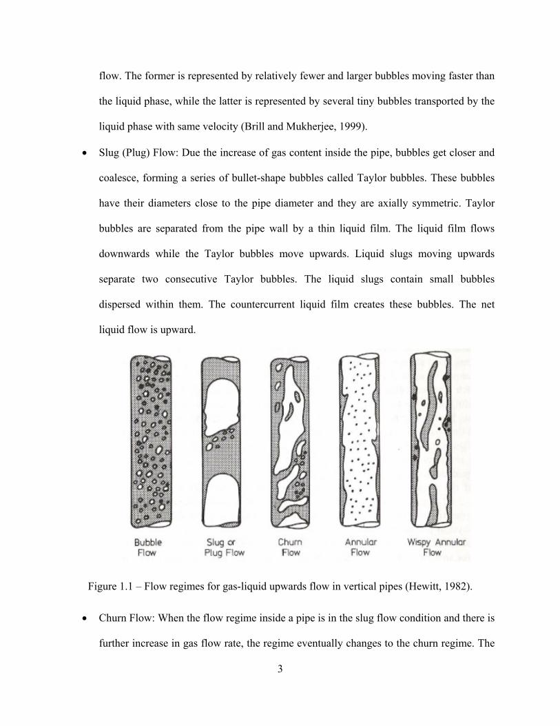
Figure 1.1 – Flow regimes for gas-liquid upwards flow in vertical pipes (Hewitt, 1982). ............. 3 

Figure 2.1 – Graphical representation of the total pressure gradient for gas-liquid flow in vertical- or near-vertical pipes (Modified after Shoham, 2006). .................................................. 11 

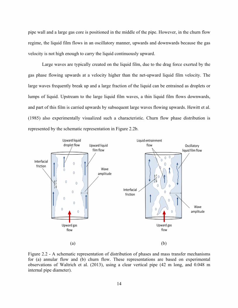
Figure 2.2 - A schematic representation of distribution of phases and mass transfer mechanisms for (a) annular flow and (b) churn flow. These representations are based on experimental observations of Waltrich et al. (2013), using a clear vertical pipe (42 m long, and 0.048 m internal pipe diameter). ................................................................................................................. 14 

Figure 2.3 – The nodal analysis technique used to predict liquid loading in gas wells. The intersection between the IPR and TPR curves to left of the minimum pressure point defines if the well is under liquid loading conditions (Lea et al., 2003). ........................................................... 20 

Figure 3.1 - Force balance for a pipe segment for churn and annular flow regimes on (a) gas core and (b) total cross-sectional area (including liquid film and gas core). ........................................ 24 

Figure 3.2 – Proposed nodal analysis technique to predict liquid loading: (a) the tangent between the IPR and TPR curves defines liquid loading initiation, and (b) gas production rate suddenly declines after time t4 as the reservoir cannot sustain steady-state two-phase flow for flow rates lower than Qmin. ............................................................................................................................. 32 

Figure 4.1 - Comparison between model and experimental results in terms of pressure gradient and liquid holdup (data from Skopich et al., 2015), for 0.0508 m (2 in) pipe diameter and superficial liquid velocities of (a) 0.01 m/s, and (b) 0.05 m/s. ..................................................... 40 

Figure 4.2 - Comparison between model and experimental results in terms of pressure gradient and liquid holdup (data from Skopich et al., 2015), for 0.102 m (4 in) pipe diameter and superficial liquid velocities of (a) 0.01 m/s and (b) 0.05 m/s. ...................................................... 42 

Figure 4.3 - Comparison between model and experimental results in terms of pressure gradient (data from Van de Meulen, 2012), for 0.127 m (5 in) pipe ID, and liquid superficial velocities of (a) 0.02 m/s and (b) 0.7 m/s. ......................................................................................................... 43 

Figure 4.4 - Comparison between model and experiments results in terms of pressure gradient (data from Zabaras et al., 2013) for 0.279 m (11 in) pipe ID, and liquid superficial velocities of (a) 0.03 m/s and (b) 0.15 m/s. ....................................................................................................... 44 

Figure 4.5 – (a) Absolute average error and (b) comparison between experimental and calculated pressure gradient for models used in this study. ........................................................................... 45 

Figure 4.6 – (a) Absolute average error, and (b) calculated and measured bottomhole pressure for the field database of Reinicke et al. (1987), for wells having tubing diameters around 0.101 m (3.976 in). ...................................................................................................................................... 47 

vii

Figure 4.7 - Comparison between simulation results using the model proposed in this study and measured wellbore pressure profile (field data from Fancher and Brown, 1963). Circles represent the measured pressures and continuous lines are the simulated pressures. Dash lines represents the depth at which a flow regime transition happened based on the simulation. .......................... 49 

Figure 4.8 - (a) Absolute average error, and (b) calculated and measured bottomhole pressure for the field database of Fancher and Brown (1963), for wells having tubing diameters around 0.0508 m (2 in). ............................................................................................................................. 50 

Figure 4.9 – Example on how Veeken et al. (2010) have defined the minimum gas flow (Qmin) that represents the liquid loading initiation. .................................................................................. 52 

Figure 4.10 – Examples on how the method of using IPR tangent to TPR curve was validated with the minimum production flow rate for wells: (a) 28a, (b) 28b in Veeken et al. (2010) database. The figure also shows the results for the prediction of liquid loading initiation using the droplet model of Turner et al. (1969). ........................................................................................... 54 

Figure 4.11 – (a) Relative error, and (b) absolute average error for the comparison between field data published by Veeken et al. (2010) for the predicted minimum flow rate for liquid loading initiation. These results show the prediction for the field data using the concept of IPR tangent to the TPR proposed, using TPR model proposed in this study and Gray (1974). Turner et al. (1969) critical flow rate is also compared to the same field data set. The angle () above the x-axis in figure (a) indicates the inclination of the well. ............................................................................. 56 

Figure 4.12 – (a) Relative error and (b) absolute average error for the comparison between field data published by Veeken et al. (2010) for the predicted minimum flow rate for liquid loading initiation when using the concept of minimum pressure of Lea et al. (2003) with the TPR model proposed in this study and Gray (1974). Figure 4.12b also includes the results previously presented in Figure 4.11b. The results for Turner et al. (1969) critical flow rate are also compared. The angle () above the x-axis in figure (a) indicates the inclination of the well....... 59 

Figure 4.13 – Simulated results shows the increase on wellbore liquid holdup over time using the proposed model with correlation for TPR proposed in this study. This increase in liquid content in the wellbore is often correlated in the field to liquid loading symptoms. ................................ 61 

Figure 4.14 – Simulated results for decline in production rate over time using the correlation for the TPR proposed in this study, and Gray (1974) correlation. The sharp and sudden change gas rate indicates the liquid loading initiation. The explanation for the large divergence between the model proposed in this study and other popular flow correlation is a consequence of the difference in predicted bottomhole pressure for low gas rates as shown in Figure 4.10. ............. 62 

Figure 4.15 – Schematic representation of the change in wellbore liquid holdup, for different times for the simulated case. ......................................................................................................... 64 

viii

Abstract

This thesis presents an improved model for gas-liquid two-phase flow in churn and

annular flow regimes for small- and large-diameter in vertical and near-vertical pipes. This new

model assumes that a net liquid film moves upward along the pipe wall and gas phase moves

upward, occupying the majority of the central part of the pipes, and forming a gas core, in both

flow regimes. The model is validated using field and laboratory experimental data from several

different studies from the literature, in terms of pressure along the wellbore or bottomhole

pressure for field conditions (for high-pressure flows in long pipes, and using hydrocarbons

fluids), and pressure-gradient and liquid holdup for experimental laboratory data, for pipe

diameters ranging from 0.0318 to 0.279 m (1.2520 to 11 in). The proposed model presents an

overall better performance when compared to several other multiphase flow models widely used

in the oil and gas industry.

This model is also tested in the application of prediction of liquid loading in gas wells.

Liquid loading is generally associated with a reduction of ultimate recovery of gas wells. Liquid

loading inception is simulated using nodal analysis technique. This study suggests that liquid

loading initiates when the Inflow Performance Relationship (IPR) curve is tangent to the TPR

curve. This study also proposes a new concept of a modified Tubing Performance Relationship

(TPR) curve in order to predict the time liquid loading initiates and when the gas well stops

flowing after reaching this condition. Field data is used for validation of this approach. The use

of conventional models shows a significant mismatch predicting the inception of liquid loading,

while the use of the tangent concept reduces this mismatch significantly.

1

1. Introduction 1, 2

Gas-liquid two-phase flow is widely existent in many industrial areas. In the chemical

processing industry, two-phase flow is encountered easily in distillation towers and direct-

contact heat exchangers. The nuclear power industry makes use of steam and water two-phase

flows, where the fluid mixture works as a coolant to absorb heat from the reactor core. In the

petroleum industry, gas-liquid two-phase flow occurs inside wellbores, risers, and pipelines,

during production and transportation of hydrocarbons.

Hewitt (1982) described that among the four possible combinations of two-phase flows

(gas-liquid, gas-solid, liquid-liquid, liquid-solid), gas-liquid two-phase flow is the most complex,

as it includes the effects of gas compressibility and the deformable interface between the phases.

For several decades, efforts have been focused on comprehending how the gas-liquid phases

interact and flow inside pipes. Depending on the gas and liquid flow rates and fractions, pipe

diameter and inclination, fluid properties, and conduit configurations, these two phases behave

differently. The complication occurs due to the fact that the forces acting on the fluids such as

buoyancy, inertia, viscosity, and surface tension vary as a function of phase distribution and

conduit size and shape. The geometric configurations the flowing mixtures exhibit in the conduit

are classified as flow regimes (this study uses the term “flow regime”, which is essentially the

same as “flow patterns” as preferred by some other studies).

1This chapter previously appeared as E. Pagan, W. C. Williams, S. Kam, P. J. Waltrich, Modeling Vertical Flow in Churn and Annular Flow Regimes in Small- and Large-Diameter Pipes, Paper Presented and Published at BHR Group’s 10th North American Conference on Multiphase Technology 8-10th June 2016. It is reprinted by permission of Copyright © 2016 BHR Group. See Appendix for more details. 2Section 1.2 of this chapter previously appeared as Erika V. Pagan, Wesley Williams, and Paulo J. Waltrich, A Simplified Transient Model to Predict Liquid Loading in Gas Wells, Paper SPE-180403-MS presented at the SPE Western Regional Meeting held in Anchorage, Alaska, USA, 23-26 May 2016. It is reprinted by permission of Copyright 2016, Society of Petroleum Engineers Inc. Copyright 2016, SPE. Reproduced with permission of SPE. Further reproduction prohibited without permission. See Appendix for more details.

2

For vertical and near-vertical pipes, these flow regimes are commonly classified as

bubble (bubbly or dispersed-bubble), slug, churn and annular flow regimes.

Flow Regimes 1.1

The presence of two phases flowing through a pipe leads to the existence of flow

regimes, which are characterized by the geometric distribution of the fluid phases in a pipe

section. Many researches have tried to recognize and define these two-phase configurations

using different methods, such as visualization through transparent pipes, photographic methods,

X-radiography measurements, and multibeam gamma densitometry. The principle of each

method and the problems in their application are summarized by Hewitt (1982). The

photographic method using high speed camera is widely used, since it allows for flow

visualization, and it is more reliable than only direct visual observation.

Diverse interpretations on visualization of flow behavior by different researchers have led

to a lack of agreement in the description and classification of the flow regimes. The present study

presents the generally encountered classification for flow regimes for gas-liquid flowing upward

in a vertical and near-vertical pipe. Keeping a constant liquid flow rate in the pipe, and

increasing the gas flow rate, the regimes change from bubble flow at low gas flow rate to slug

flow, then to churn flow, and finally to annular flow at high gas rates. When flow configuration

is in the annular flow regime, an increase in liquid rate leads to another flow regime called wispy

annular flow. These regimes are represented by Figure 1.1, and are characterized as follows:

Bubble (dispersed-bubble) Flow: The gas phase is present in form of dispersed bubbles

uniformly distributed in the continuous liquid phase. This regime occurs when there are

high liquid velocities and low gas velocities flowing through the tubing. Both phases

move upwards. This regime can be further classified into bubbly or dispersed-bubble

3

flow. The former is represented by relatively fewer and larger bubbles moving faster than

the liquid phase, while the latter is represented by several tiny bubbles transported by the

liquid phase with same velocity (Brill and Mukherjee, 1999).

Slug (Plug) Flow: Due the increase of gas content inside the pipe, bubbles get closer and

coalesce, forming a series of bullet-shape bubbles called Taylor bubbles. These bubbles

have their diameters close to the pipe diameter and they are axially symmetric. Taylor

bubbles are separated from the pipe wall by a thin liquid film. The liquid film flows

downwards while the Taylor bubbles move upwards. Liquid slugs moving upwards

separate two consecutive Taylor bubbles. The liquid slugs contain small bubbles

dispersed within them. The countercurrent liquid film creates these bubbles. The net

liquid flow is upward.

Figure 1.1 – Flow regimes for gas-liquid upwards flow in vertical pipes (Hewitt, 1982).

Churn Flow: When the flow regime inside a pipe is in the slug flow condition and there is

further increase in gas flow rate, the regime eventually changes to the churn regime. The

4

slugs are continuously destroyed by the high local concentration of gas phase,

consequently the Taylor bubbles are distorted by the liquid phase. This regime is

represented by a chaotic motion of the phases, since there is no clear boundary between

the phases. More details about this flow regime are discussed later in this section.

Annular Flow: This flow is characterized by a thin wavy layer of liquid near the pipe wall

and a relatively fast gas core flowing through the center of the pipe. Entrained liquid

droplets are generally present in the gas core and gas bubbles are generally entrained in

the liquid film. More details about this flow regime is also presented later in this section.

Wispy Annular: In this flow, droplets coalesce in the core creating large lumps or streaks,

called wisps, due an increase of liquid rate.

In order to predict the pressure gradient in a wellbore, various multiphase flow models

are used in the literature. They often use different sub-models or correlation coefficients for each

flow regime because each regime has a unique hydrodynamic behavior. Thus, it is essential to

develop accurate models for a wide range of flow regimes.

Waltrich (2012) stated that churn flow regime is generally encountered in producing gas

wells under liquid loading conditions. However, Hewitt (2012) has described that churn flow

regime is far less studied, thus less understood, than other flow regimes in vertical two-phase

flows. The reason for the lack of mechanistic models to predict the hydrodynamic properties of

churn flow is due to the highly chaotic and disordered nature of this flow regime (Kaya et al.,

2001). According to Kaya et al. (2001), many times hydrodynamic models for slug flow regimes

are used to model churn flow without any modifications. Other studies have suggested few

modifications on previous validated slug flow models in order to develop a model to churn flow

(Tengesdal et al., 1999).

5

Two-Phase Flow Modeling in Small and Large Diameter Pipes 1.2

Although there are numerous studies to model the pressure gradient and liquid holdup in

vertical pipes, most of them were originally developed for small pipe diameters (smaller than

0.1016 m (4 in)) (Poettmann and Carpenter, 1952; Hagedorn and Brown, 1965; Beggs and Brill,

1973; Gray, 1974). Some of the commercial multiphase flow simulators, widely used in the

industry, have long and complex codes, most of which are tuned with field data and are not open

to the public, and thus the understanding of the underlying assumptions and limitations behind

such codes is limited.

Recent studies (Omebere-Yari and Azzopardi, 2007; Ali, 2009; Van der Meulen, 2012;

Zabaras et al., 2013) have attempted to capture the behavior of two-phase flow in large-diameter

vertical pipes (ID ≥ 0.127 m (5 in)). Some of these studies show experimentally that churn flow

regime is commonly observed for a wide range of gas-liquid ratios for two-phase flows when the

pipes have large diameters. It was also observed, more importantly, that the behavior of flow

regimes is significantly different in large pipe diameters. For instance, slug flow regime is not

experimentally observed in large pipe diameters, when it is expected to occur in small pipe

diameters at the same flowing conditions (Omebere-Yari and Azzopardi, 2007; Ali, 2009; Van

der Meulen, 2012; Zabaras et al., 2013).

The Bureau of Ocean Energy Management (2010) requires Worst Case Discharge

(WCD) calculations prior to all wells being permitted in the Gulf of Mexico. During drilling

activities, diameters larger than 0.254 m (10 in) are present in many portions of the well

configuration. The use of multiphase flow models for large pipe diameters is essential to the

calculation of WCD for offshore wells. The extension of existing mechanistic models and flow

correlations, built based on small-diameter experiments, however, is still uncertain. SPE (2015)

6

raised the same concerns by stating that further research for correlations applicable at high flow

rates in large pipe diameters is needed. Zabaras et al. (2013) also discussed the need of two-

phase flow models for large diameter pipes for gas-lift applications within offshore risers.

Multiphase flow models are also suggested by some investigators to be used for the

estimation of liquid loading initiation in gas wells (Skopich et al., 2015; Waltrich et al., 2015b).

Liquid loading is generally defined as the inability of a producing gas well to lift the coproduced

liquids up the tubing, resulting in liquid accumulation in the wellbore. One of the main problems

associated with liquid loading is the sudden drop in gas production rates or “death” of the well.

Decline curve analysis often fails to predict the sudden drop in gas production observed in the

field (Lea et al., 2003), and this mismatch in production forecasting can have a significant impact

on the prediction of ultimate recovery for gas wells. Thus, liquid loading can be associated with a

reduction of ultimate recovery of gas wells. Therefore, it is clear to conclude that the

development of a model to predict the production forecast for gas wells should include the liquid

loading phenomenon and its transient effects.

Based on the need of more studies on churn flow regime and further development of two-

phase flow models for large pipe diameters, this study proposes a model for gas-liquid two-phase

flows that can be applied to churn and annular flow regimes in vertical and near-vertical pipes,

for small and large pipe diameters. This study also proposes the use of this model to predict

production forecast of gas wells, including the transient effects before and after liquid loading

initiation, by use of the nodal analysis technique.

Objectives 1.3

The objective of this thesis is to develop a model for gas-liquid two-phase flow in churn

and annular flow regimes for small- and large-diameter in vertical and near-vertical pipes. This

7

model is intended to be used by the oil and gas industry for several different applications such as

gas-lift operations, production of gas-condensate wells, Worst Case Discharge calculations,

prediction of liquid loading initiation, and high-gas-volume fraction two-phase flows in general.

To accomplish this objective, the following tasks are carried out:

Literature review of gas-liquid flow in vertical and near-vertical pipes for a broad range

of pipe sizes.

Collect experimental and field data available in the literature in terms of bottomhole

pressure, pressure profile along the wellbore, pressure gradient and liquid holdup for

vertical and near-vertical pipes, particularly for churn and annular flow regimes.

Develop a model for churn and annular flow regimes, for vertical and near-vertical two-

phase flows for tubes of small and larger diameters.

Compare the model proposed in this study with the state-of-the-art models and

commercial packages.

Develop a model that can predict the transient behavior of liquid loading in gas wells.

Describing the symptoms related to liquid loading often observed in the field using the

model developed in this study.

Thesis Outline 1.4

This thesis is divided into five chapters. Chapter 1 shows the problem and the motivation

of this thesis, as well as the importance of this research and its objectives. The following chapters

are divided in two main sections, the first section is related to the development of the multiphase

flow model for churn and annular flow, and the second section is related to the application of this

model to the prediction of liquid loading initiation. Chapter 2 reviews the basic theory on two-

phase flow in vertical and near-vertical pipes, as well as, details the concepts of churn and

8

annular flows. In addition, it discusses the current methods and their limitations in prediction of

liquid loading in gas wells. Chapter 3 describes how the model for churn and annular flow for

vertical and near-vertical pipes was developed. It also presents the concept this study suggests to

be applied to predict the inception of liquid loading in gas wells. Chapter 4 presents the results of

the comparison of the churn and annular model simulations on the prediction of pressure gradient

and liquid holdup using several different experimental data, and on the prediction of bottomhole

pressure, and pressure along the wellbore using field data. It also presents the simulations using

different models and correlations available in the literature. These simulations were performed

using PIPESIM software (PIPESIM, 2013). In addition to this, Chapter 4 presents the results of

the prediction of liquid loading initiation using the concept proposed in this study. Finally,

chapter 5 summarizes the content of this study as well as presents the conclusions obtained from

this investigation, and suggests recommendations for future work.

9

2. Literature Review 1, 2

This chapter is subdivided into two main sections. The first section outlines the

fundamentals of two-phase flow. The second section presents a literature review based on the

current models used in the prediction of liquid loading initiation.

Two-Phase Flow Modeling 2.1

For a clear understanding of the content of this thesis, the fundamentals of two-phase

flow is briefly presented. In the next sections, the concepts of liquid holdup, void fraction,

pressure gradient, superficial velocities, and flow regimes are explained.

2.1.1 Liquid Holdup

Void fraction (α) is defined as volumetric fraction of gas phase contained in a section of a

pipe. Void fraction is commonly defined by the following expression,

(2.1)

where Vg is the volume of gas present in a certain pipe segment, and V is the total volume of the

pipe segment.

The liquid holdup is the complement of void fraction (or liquid fraction in the considered

pipe segment), which is represented by the following expression,

1 (2.2)

1Section 2.1 of this chapter previously appeared as E. Pagan, W. C. Williams, S. Kam, P. J. Waltrich, Modeling Vertical Flow in Churn and Annular Flow Regimes in Small- and Large-Diameter Pipes, Paper Presented and Published at BHR Group’s 10th North American Conference on Multiphase Technology 8-10th June 2016. It is reprinted by permission of Copyright © 2016 BHR Group. See Appendix for more details. 2Section 2.2 of this chapter previously appeared as Erika V. Pagan, Wesley Williams, and Paulo J. Waltrich, A Simplified Transient Model to Predict Liquid Loading in Gas Wells, Paper SPE-180403-MS presented at the SPE Western Regional Meeting held in Anchorage, Alaska, USA, 23-26 May 2016. It is reprinted by permission of Copyright 2016, Society of Petroleum Engineers Inc. Copyright 2016, SPE. Reproduced with permission of SPE. Further reproduction prohibited without permission. See Appendix for more details.

10

The prediction of liquid holdup in a pipe segment is one of the most important parameters

in the determination of the pressure gradient for two-phase flow in pipes.

2.1.2 Pressure Gradient

Pressure gradient is defined as the pressure drop per unit length of pipe. It is represented

by the term -dp/dl, where dp is the pressure drop and dl is the unit length of the pipe. The

negative sign is usually used in front of the term to turn the term positive, since the pressure

generally drops for upward flow in pipes (Shoham, 2006).

The total pressure gradient is commonly represented by the sum of three components:

pressure gradient due to friction, pressure gradient due to gravitation effects, and pressure

gradient due to flow acceleration. The total pressure gradient can be represented by the

following equation,

(2.3)

where –dp/dl is the total pressure gradient, -(dp/dl)f is the frictional component, -(dp/dl)g is the

gravitational component, -(dp/dl)acc is the accelerational component.

The pressure gradient equation for steady-state flow in pipes uses the principles of mass

and momentum conservation. For two-phase flow, the frictional component results from the

pressure drop due to friction losses at the pipe wall, as well as the friction due to the shear stress

between the phases. The gravitational component accounts for the elevation change of the fluids

in the gravitational field. The accelerational component is a consequence of the changes in

velocities along the pipe length. For adiabatic flows and low flow velocities, this last term is

usually very small in comparison to the first two terms, and consequently, is often neglected

(Brill and Mukherjee, 1999). In this study, the accelerational component is also neglected.

11

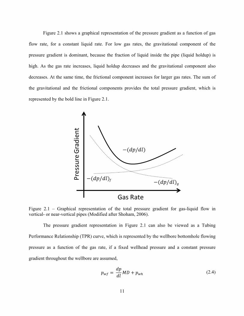
Figure 2.1 shows a graphical representation of the pressure gradient as a function of gas

flow rate, for a constant liquid rate. For low gas rates, the gravitational component of the

pressure gradient is dominant, because the fraction of liquid inside the pipe (liquid holdup) is

high. As the gas rate increases, liquid holdup decreases and the gravitational component also

decreases. At the same time, the frictional component increases for larger gas rates. The sum of

the gravitational and the frictional components provides the total pressure gradient, which is

represented by the bold line in Figure 2.1.

Figure 2.1 – Graphical representation of the total pressure gradient for gas-liquid flow in vertical- or near-vertical pipes (Modified after Shoham, 2006).

The pressure gradient representation in Figure 2.1 can also be viewed as a Tubing

Performance Relationship (TPR) curve, which is represented by the wellbore bottomhole flowing

pressure as a function of the gas rate, if a fixed wellhead pressure and a constant pressure

gradient throughout the wellbore are assumed,

(2.4)

12

where is the wellbore flowing bottomhole pressure, is the wellbore measured depth, and

is the wellhead pressure.

The shape of the TPR curve depends on the gas and liquid rates, as well as on the

individual components in the production system (i.e., completions configuration, wellbore and

flowline length and diameter, choke valves, among others). These components are responsible

for the flow pressure changes from the reservoir to the surface. The liquid and gas volumetric

flow rate can be represented in terms of superficial velocities. The definition of superficial

velocity is described next.

2.1.2.1 Superficial Velocities

The superficial velocity of the liquid phase ( ) or the gas phase ( ) is the ratio of the

volumetric flow rate of the phase ( for the liquid phase or for the gas phase) divided by the

total cross sectional area of the pipe (A). The liquid superficial velocity is defined as,

(2.5)

and the gas superficial velocity as,

(2.6)

The superficial velocity characterizes the velocity that would have happened if only one

phase is flowing in a pipe segment. A dimensionless form of the superficial velocities for liquid

and gas are represented by the Froude number, defined by the following equations (Hewitt and

Wallis, 1963):

∗.

(2.7)

13

∗

.

(2.8)

where is the gas-phase density, is the liquid-phase density, is the gravitational constant,

and is the diameter of the pipe.

The model proposed in this study applies the mass and momentum conservation

equations for churn and annular flows. Therefore, before applying the conservation equations, it

is important to characterize the main features of each flow regime. The next two sections

describe the main details and the differences for churn and annular flows.

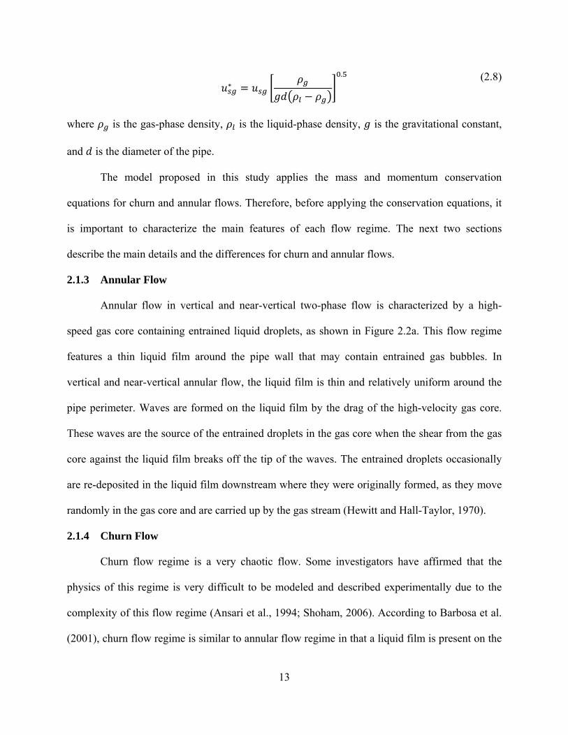
2.1.3 Annular Flow

Annular flow in vertical and near-vertical two-phase flow is characterized by a high-

speed gas core containing entrained liquid droplets, as shown in Figure 2.2a. This flow regime

features a thin liquid film around the pipe wall that may contain entrained gas bubbles. In

vertical and near-vertical annular flow, the liquid film is thin and relatively uniform around the

pipe perimeter. Waves are formed on the liquid film by the drag of the high-velocity gas core.

These waves are the source of the entrained droplets in the gas core when the shear from the gas

core against the liquid film breaks off the tip of the waves. The entrained droplets occasionally

are re-deposited in the liquid film downstream where they were originally formed, as they move

randomly in the gas core and are carried up by the gas stream (Hewitt and Hall-Taylor, 1970).

2.1.4 Churn Flow

Churn flow regime is a very chaotic flow. Some investigators have affirmed that the

physics of this regime is very difficult to be modeled and described experimentally due to the

complexity of this flow regime (Ansari et al., 1994; Shoham, 2006). According to Barbosa et al.

(2001), churn flow regime is similar to annular flow regime in that a liquid film is present on the

14

pipe wall and a large gas core is positioned in the middle of the pipe. However, in the churn flow

regime, the liquid film flows in an oscillatory manner, upwards and downwards because the gas

velocity is not high enough to carry the liquid continuously upward.

Large waves are typically created on the liquid film, due to the drag force exerted by the

gas phase flowing upwards at a velocity higher than the net-upward liquid film velocity. The

large waves frequently break up and a large fraction of the liquid can be entrained as droplets or

lumps of liquid. Upstream to the large liquid film waves, a thin liquid film flows downwards,

and part of this film is carried upwards by subsequent large waves flowing upwards. Hewitt et al.

(1985) also experimentally visualized such a characteristic. Churn flow phase distribution is

represented by the schematic representation in Figure 2.2b.

   

(a) (b)

Figure 2.2 - A schematic representation of distribution of phases and mass transfer mechanisms for (a) annular flow and (b) churn flow. These representations are based on experimental observations of Waltrich et al. (2013), using a clear vertical pipe (42 m long, and 0.048 m internal pipe diameter).

15

The churn flow regime has been known to occur between the slug and the annular flow

regimes, although a direct transition from slug or even from bubbly flow directly to annular flow

may happen at very high liquid flow rates (Jayanti and Hewitt, 1992). Some researchers do not

recognize churn flow as a separate flow regime because of its similarity with annular flow. Many

other researchers believe that this configuration is simply a transition regime. For instance, Taitel

et al. (1980) and Dukler and Taitel (1986) describe churn flow regime as an entrance

phenomenon preceding a downstream stable slug flow for a pipe of enough length. Waltrich et

al. (2013), however, recently stated that the churn flow regime exists and should be admitted as a

separate regime. Their conclusion was based on experimental observations, through video

recordings and liquid holdup measurements by using a 42 m long, 0.048 m internal diameter,

vertical tube system.

2.1.5 Correlations Available in the Literature

There are several correlations available in the literature developed to model the

hydrodynamics of two-phase flows in wellbores under different flow regimes. Some of these

correlations are well accepted by the oil and gas industry and widely used to estimated pressure

gradient in wellbores.

In this study, some of these correlations are used to simulate the data collected in order to

compare the performance of the model proposed in this study in relation to other correlations

currently available in software packages.

The correlations selected for the comparison in this study (Duns and Ros, 1963; Gray,

1974; Ansari et al., 1994; OLGA, 2000) are included in PIPESIM software (PIPESIM, 2013).

This section carries out a brief literature review on these correlations, based on the conditions of

which each flow correlation used in this study was developed and validated.

16

2.1.5.1 Duns and Ros (1963) Correlation

Duns and Ros (1963) developed their empirical correlations based in three different

regions determined by them according to the gas rate. Region I is a region of low gas rates,

which is composed by a continuous liquid phase comprising bubble flow, plug flow (similar to

slug flow – more stable bullet-shaped gas plugs in the continuous liquid phase) and part of the

froth-flow (also called churn) regime. Region II is a region of intermediate gas rates, which the

continuous phase alternate between liquid and gas phases. Region II comprises slug flow and the

remainder of the froth-flow regime. Region III is a region of high gas rate, which is composed by

a continuous gas phase comprising mist-flow regime.

Duns and Ros (1963) stated that their correlation can be applied over an extensive range

of field operating conditions. Their correlation was validated using approximately 20,000 data

points from about 4,000 gas-liquid two-phase flow tests (Li, 2013). Besides water, other fluids

with different densities, surface tension and viscosity were also used in their experiments as

lubricating oil, gas oil and mineral spirit (Li, 2013). The data were measured in a vertical pipe

section of 10 m (32.8 ft) height and nominal internal diameters of 0.032, 0.0802, and 0.1423 cm

(1.2598, 3.1575, and 5.6024 in) (Takacs, 2001). Superficial liquid velocities ranged from 0 to

100 m/s, and superficial gas velocities from 0 to 32 m/s (Li, 2013). Water cut ranged from 0 to

100 % (Takacs, 2001).

2.1.5.2 Gray (1974) Correlation

The Gray (1974) empirical correlation was developed for vertical gas wells with

coproducing liquids. Flow is treated as single-phase. Thus, no flow regime is considered. They

used 108 test data from wells, in which 88 of these were reported to coproduce some liquid (Li,

2013). Their results for prediction of pressure gradient were superior to the predictions using

17

conventional dry gas models. However, the accuracy of the Gray (1974) method is still uncertain

for some conditions (Li, 2013): for mixture velocity (sum of superficial liquid velocity and

superficial liquid velocity) greater than 15.24 m/s (50 ft/s), for nominal pipe diameters greater

than 0.0889 cm (3.5 in), liquid condensate and gas ratio greater than 2.81x104 m3/sm3 (50

bbl/MMscf), and water and gas ratio greater than 2.81x105 m3/sm3 (5 bbl/MMscf).

2.1.5.3 Ansari et al. (1994) Correlation

The Ansari (1994) mechanistic model is composed of a set of independent correlations to

predict pressure drop and liquid holdup in bubble, slug, and annular flow regimes, as well as by a

model to predict the transition between these flow regimes. Churn flow was not considered.

Their method was validated using Tulsa Fluid Flow Project (TUFFP) well data bank containing

1,712 well cases with a wide range of conditions as nominal diameter varying from 0.0254 to

0.2032 m (1 to 8 in), oil rates from 0 to 4,300 sm3/d (0 to 27,000 stb/d), gas rates from 0.46 to

33,500 Msm3/d (1.5 to 110,000 Mscf/d), and oil gravity from 9.5 to 112 oAPI.

2.1.5.4 OLGA (2000) Correlation

The OLGA (2000) mechanistic model was developed for predictions of steady-state

pressure drop, liquid holdup, and flow regime transitions (Bendiksen et al., 1991). OLGA (2000)

model was validated using SINTEF Two-Phase Flow Laboratory (near Trondheim, Norway)

data, as well as other data from literature and field. SINTEF experimental loop was designed to

operate at conditions close to field conditions. The loop is 800 m long with 0.0254 m (8 in)

internal diameter. Naphtha, diesel oil, or lube oil was used as liquid phase. Nitrogen was used as

gas phase. Pressures ranged from 20 to 95 barg (Rygg and Gilhuus, 1990). Superficial liquid

velocities up to 4 m/s and superficial gas velocities up to 13 m/s were tested (PIPESIM, 2013).

The model uses three separate mass continuity equations for gas, liquid bulk, and liquid droplets.

18

In addition, one momentum balance equation for gas and liquid droplets, and other for the liquid

film. One energy conservation equation is also included in the model (Bendiksen et al., 1991).

Their determination of flow regime is based in two groups: distributed flow and separated flow.

The former includes bubble and slug flow regimes, and the latter includes what they call

stratified and annular mist flow regimes.

Liquid Loading 2.2

This section discusses the current methods and their limitations on prediction of the

inception of liquid loading in gas wells. Liquid loading is a phenomenon that happens to all gas

wells, which co-produce some liquids, at some stage of their production life cycle (Lea et al.,

2003). This phenomenon is generally associated with a reduction of ultimate recovery of gas

wells. In order to accurately forecast gas wells production, prediction of liquid loading initiation

is necessary.

2.2.1 Turner et al. (1969) Droplet Model

Models commonly used to predict the initiation of liquid loading utilize the idea of

critical gas velocity to determine when liquid loading starts. The most widely accepted method to

predict liquid loading initiation is the droplet transport model of Turner et al. (1969). In their

approach, the balance between downward gravitational force and upward gas drag force on a

liquid droplet is solved to determine the minimum velocity (umin) to lift the largest droplet

flowing with the gas stream, given by the following expression,

5.46⁄

(2.9)

where σ is the surface tension (in N/m), ρg is the gas density (in kg/m3) and ρl is the liquid

density (in kg/m3).

19

The development of Equation (2.9) by Turner et al. (1969) was based on a comparison

between their droplet model and a liquid film transport model. Both models were compared to

field data, and the droplet model showed a superior performance in predicting liquid loading.

However, the field data collected by Turner et al. (1969) only included surface measurements,

and key variables such as surface tension and fluid densities were simply estimated based on

generic fluid property correlations. Another important information missing in their work was the

fact that the work of Turner et al. (1969) did not clearly define how they classified wells as

“loaded” or “unloaded”. Furthermore, Westende et al. (2007) and Waltrich et al. (2105a) have

shown experimentally that even for gas velocities lower than the minimum critical velocity of

Turner, given by Equation (2.9), liquid droplets flow upwards and not downwards as suggested

by Turner et al. (1969). Another limitation of the model proposed by Turner et al. (1969) is the

fact that Equation (2.9) only calculates the minimum flow rate for liquid loading initiation. This

method cannot be used to simulate the transient effects of liquid loading in gas wells, i.e., the

time the well starts suffering from liquid loading, and when the gas well stops production after

liquid loading initiation.

2.2.2 Minimum Pressure Point and Nodal Analysis

Another commonly used method to predict liquid loading initiation includes the concept

of the minimum pressure point in the wellbore curve, as shown in Figure 2.3 (Lea et al., 2003).

This concept assumes that when the reservoir Inflow Performance Relationship (IPR) curve

intersects the Tubing Performance Relationship (TPR) curve to the left or at the minimum

pressure point, liquid loading is initiated. This method is often correlated to the transition

between annular to churn (or intermittent) flow regime based on the minimum pressure of the

TPR curve, which is also used as criterion for liquid loading initiation in some studies (Skopich

20

et al., 2015; Riza et al., 2015). In Figure 2.3, the difference between IPR1 and IPR2 is the average

reservoir pressure, where it is known that the reservoir presssure naturally depleats as

consequence of the gas production.

Figure 2.3 – The nodal analysis technique used to predict liquid loading in gas wells. The intersection between the IPR and TPR curves to left of the minimum pressure point defines if the well is under liquid loading conditions (Lea et al., 2003).

A limitation for this method is that it cannot explain the production from reservoirs with

low permeability, wich normally present IPR curves that intercepts the TPR curve to the left of

the point of minimum pressure, and these wells can still flow without suffering from liquid

loading symptoms (Lea et al., 2003). Thus, the concept of minimum pressure may not be the

most appropriate to predict liquid loading initiation since it may work for some reservoirs, but

not for others, depending, for instance, on the reservoir permeability.

2.2.3 Coupled Reservoir/Wellbore Modeling

Recently, some investigators (Zhang et al., 2009; Yusuf et al., 2010; Hu et al., 2010) have

proposed coupled reservoir/wellbore modeling to predict liquid loading in transient conditions.

21

Although these models provide reasonable solutions for liquid loading in transient

conditions, some of these models include the use of commercial simulators or sophisticated

modeling techniques that cannot be easily implemented using simple reservoir and tubing

performance relationships. This study believes that one of the main reasons for the wide

acceptance of the droplet model of Turner is due to the fact that Equation (2.9) gives a very

simple relationship to indicate liquid loading initiation, which can be easily understood by most

engineers. Therefore, it is important to develop a simplified model to predict liquid loading under

transient conditions.

Other investigators have already proposed simplified methods to describe liquid loading

under transient conditions using simple reservoir and tubing performance relationships. For

instance, Oudeman (1990) proposed the use of multiphase reservoir performance and vertical

flow performance of the tubing to improve prediction of wet-gas-well performance and liquid

loading. To the knowledge of the authors, Oudeman’s work was one of the first attempts to

couple the reservoir performance to the tubing flow performance in order to explain liquid

loading in gas wells under transient conditions. Following his approach, Dousi et al. (2006) has

proposed the use of reservoir inflow performance coupled with a tubing flow performance curve

to explain a process of water buildup and drainage in gas wells under transient liquid loading

conditions. Dousi et al. (2006) also defined a condition called “metastable flow” as subcritical

rates that a gas well would flow under liquid loading conditions.

Some authors (Chupin et al., 2007; Veeken et al., 2010; Whitson et al., 2012) have also

shown the observation of metastable flow using field data. More recently, Limpasurat et al.

(2015) have proposed the use of a new boundary condition for a coupled reservoir/wellbore

modeling method that was validated with field data. These authors concluded that this new

22

boundary condition improves the prediction of transient effects for gas wells under liquid loading

and also enhances the model previously proposed by Dousi et al. (2006). They also concluded

that this new boundary condition can show the metastable flow observed in the field, as

originally suggested by Dousi et al. (2006). However, Dousi et al. (2006) and Limpasurat et al.

(2015) still have to use the minimum velocity criterion of Turner et al. (1969) to trigger liquid

loading conditions.

Although the recent attempts of coupled reservoir/wellbore modeling have shown

improvements on the understanding of liquid loading, simplified transient models are still

exceptions rather than the norm. With the exception of the models using proprietary codes

(which do not fully disclose all assumptions and details about their approach), all the other

models discussed in this study use the minimum velocity criterion of Turner et al. (1969) to

trigger liquid loading, even though the accuracy of Turner’s droplet model has been recently

questioned by many authors (Oudeman, 1990; Westende et al., 2007; Veeken et al., 2010;

Skopich et al., 2015). Thus, a simplified model might encourage engineers to replace the use of

the widely accepted model of Turner for more accurate methods that are as simple as Turner’s

approach.

23

3. Models Description 1, 2

This chapter is divided into two main sections. The first section describes the model

proposed in this study for churn and annular flow. The second main section presents the concept

for liquid loading inception prediction proposed in this study.

Churn and Annular Flow Modeling 3.1

This study proposes a model for churn and annular flows in small and large diameters, in

vertical and near-vertical pipes. This model is based on an approach originally proposed by

Jayanti and Brauner (1994) for the churn flow regime in vertical pipes validated for small

diameters.

3.1.1 Momentum Equations

Figure 3.1 shows the force balance concept applied to churn and annular flows in this

study. The inner control volume (Figure 3.1a) is used for the gas core, and the outer control

volume (Figure 3.1b) is used for the entire gas and liquid phase in the cross-sectional area of the

pipe. The liquid entrainment, in the gas core, for both churn and annular flow regimes, is

assumed to be part of the liquid film, and the gas entrainment in the liquid film is neglected. In

experimental observations (Hewitt et al., 1985), only few gas bubbles are observed in the liquid

film.

Figure 3.1a illustrates the forces acting on the gas core segment with the cross-sectional

area Ac and length dl.

1Section 3.1 of this chapter previously appeared as E. Pagan, W. C. Williams, S. Kam, P. J. Waltrich, Modeling Vertical Flow in Churn and Annular Flow Regimes in Small- and Large-Diameter Pipes, Paper Presented and Published at BHR Group’s 10th North American Conference on Multiphase Technology 8-10th June 2016. It is reprinted by permission of Copyright © 2016 BHR Group. See Appendix for more details. 2Section 3.2 of this chapter previously appeared as Erika V. Pagan, Wesley Williams, and Paulo J. Waltrich, A Simplified Transient Model to Predict Liquid Loading in Gas Wells, Paper SPE-180403-MS presented at the SPE Western Regional Meeting held in Anchorage, Alaska, USA, 23-26 May 2016. It is reprinted by permission of Copyright 2016, Society of Petroleum Engineers Inc. Copyright 2016, SPE. Reproduced with permission of SPE. Further reproduction prohibited without permission. See Appendix for more details.

24

 

(a) (b) Figure 3.1 - Force balance for a pipe segment for churn and annular flow regimes on (a) gas core and (b) total cross-sectional area (including liquid film and gas core).

The net flow rates of both gas and liquid phases are upward, and the gas phase moves

faster than the liquid phase. Thus, shear stress at the interface between the gas and liquid phases,

τi, is introduced to consider the interaction between the phases. Figure 3.1b illustrates the forces

acting on the total cross-sectional area of the pipe A, which is the sum of the cross-sectional areas

of the gas core, Ac, and liquid film, Af. The interaction between the liquid film and the wall is

considered by the shear stress, τw.

The momentum (force) balance equations to the inner and outer control volumes are

given, respectively by (if the acceleration term is negligible) (Jayanti and Brauner, 1994),

4

√ (3.1)

4

1 (3.2)

where dp/dl is the pressure gradient for the pipe segment, d is the diameter of the pipe, θ

is the inclination angle (i.e., θ = 90o, if vertical), α is the void fraction, ρg and ρl are the gas and

25

liquid densities, τi is the interfacial shear stress, τw is the wall shear stress, and g is the

gravitational acceleration.

The two momentum balance Equations (3.1) and (3.2) are solved for the pressure

gradient and void fraction. The solution of these two equations requires the calculations of the

interfacial shear stress (τi) and the wall shear stress (τw). The procedure to calculate τi and τw is

presented in the next section.

A caution must be taken during the application of this model for pipes with large

inclination angles, because churn flow is gradually suppressed with increasing inclination angle,

completely disappearing at an angle of between 20 and 30 degrees from vertical direction

(Jayanti and Brauner, 1994). Therefore, the model proposed here is intended to provide

reasonable results for inclination angles up to 15 degrees (i.e., 75 o≤ θ ≤90o).

3.1.2 Wall and Interfacial Shear Stress

In the churn flow regime, the liquid motion is oscillatory. However, the net liquid rate is

upward. Thus, Jayanti and Brauner (1994) proposed that the average wall shear stress should be

calculated based on the net liquid flow rate, neglecting the variation with time. As in the annular

flow regime, the net liquid film flows always upward along the pipe wall. Thus, the wall shear

stress, τw, is calculated from the following relationship for both annular and churn flow regimes,

12 1

(3.3)

where is the superficial liquid velocity, and is the friction factor within the liquid film. This

equation represents wall shear stress for single-phase flow, considering only the liquid phase is

in contact to the pipe wall. For Reynolds number on the liquid film ( ) smaller than 2,100

(laminar flow), the Fanning friction factor for laminar flow is used,

26

16

(3.4)

and for greater than 2,100 (turbulent flow), Blasius equation for smooth pipes is used,

0.079

. (3.5)

where,

(3.6)

where is the liquid-phase viscosity. includes the actual liquid film velocity within the

film ( ), which is given by,

1

(3.7)

The interfacial shear stress between the gas core and the liquid film is calculated using

Equation (3.8), which is analogous to Equation (3.3),

12

(3.8)

where is the superficial gas velocity. Equation (3.8) can be used since the gas velocity is

generally much larger than the liquid velocity when the fluids are flowing under churn or annular

flow regimes. Thus, the liquid velocity is neglected, and the interfacial shear stress is calculated

based on single-phase gas flow.

Based on an analysis from the experimental results of Govan et al. (1991), Jayanti and

Brauner (1994), which developed their model for churn flow only, suggest that the interfacial

friction factor ( should be calculated by the average of two previously published correlations,

represented by , and , as follow,

27

12 , , (3.9)

where , was originally an empirical correlation proposed by Wallis (1969) assuming thin

liquid films in pipes and , was originally an empirical correlation proposed by Bharathan et al.

(1978). The present study uses the same average presented in Equation (3.9) for calculation of

interfacial friction factor ( ) for both churn and annular flow regimes. However, for , the

correlation of Bharathan and Wallis (1983) is used instead, as suggested by Alves (1994). This

correlation provides best results for churn and annular flow regimes, and it is given by,

, 0.005 10 . .

∗∗ 14

. .∗

(3.10)

where

∗ (3.11)

and is the surface tension between gas and liquid. Furthermore, this study proposes the use of

the general equation for interfacial friction factor proposed by Wallis (1969) for , as given by,

, 0.005 1 300 (3.12)

where /D is the dimensionless liquid film thickness in the pipe. This last term can easily be

represented in terms of void fraction ( ) since void fraction can be interpreted by the cross-

sectional area of the gas core, Ac, divided by the cross-sectional area of the pipe A. Thus, this

study proposes Wallis (1969) modified interfacial friction factor without assumption of thin

liquid film in pipes for churn flow regime, given by,

, 0.005 0.75 1 √ (3.13)

28

and Wallis (1969) modified interfacial friction factor equation with assumption of thin liquid

film in pipes for annular flow regime, given by,

, 0.005 0.375 1 (3.14)

3.1.3 The Churn to Annular Flow Transition

The transition from churn to annular flow in this study uses two different criteria

depending on the pipe size. For pipe diameters equal to and smaller than 0.0508 m (2 in), the

flow reversal criterion (assumption that all liquid film that was flowing in both upward and

downward directions starts to flow only upwards) proposed by Wallis (1969) is used. This

commonly used criterion can be easily observed experimentally and offers simple relationships

to determine the transition from churn to annular flow regimes (Hewitt and Wallis, 1963;

Pushkina and Sorokin, 1969; Taitel et al., 1980). This criterion states that this transition occurs

when the dimensionless superficial gas velocity ∗ equals to the unit (Waltrich et al., 2013), i.e.,

∗.

1 (3.15)

For pipe diameters larger than 0.0508 m (2 in), the condition for flow reversal is used as

suggested by Pushkina and Sorokin (1969), which is written in terms of Kutateladze number

( ),

. . (3.16)

where the annular flow occurs when ≥ 3.2, and the churn flow occurs when is < 3.2.

3.1.4 The Slug/Bubble to Churn Flow Transition

In this study, the transition from slug to churn, or bubble to churn flow, is also based on

two different criteria, depending on the pipe size. The pipe diameter criteria used here follows

29

the work of (Zabaras et al., 2013), which suggests that Taylor bubbles cannot be sustained in

vertical two-phase flows for pipe diameters larger than,

30 (3.17)

For diameters smaller or equal to dT, the model of Brauner and Barnea (1986) is used for

the slug-to-churn flow transition. According to their study, the transition occurs when the liquid

holdup in the liquid slug (hsl) falls below a minimum value of 0.48 due to increase in gas rate.

According to these authors, the excessive aeration causes the collapse of the liquid slug and the

transition to churn flow regime. The liquid holdup in the liquid slug is correlated by,

1 0.058 20.4 . 2

. .0.725 (3.18)

where fm is the mixture friction factor given by,

0.046.

(3.19)

Note that um is the mixture velocity (um = usg + usl), andl is the kinematic viscosity of the liquid

phase.

For pipe diameters larger than dT, a transition from bubble flow directly to churn flow is

observed (Zabaras et al., 2013). A modified version of the classical model of Taitel et al. (1986)

to the bubble-to-slug transition is used in this study to predict the bubble-to-churn flow

transition. Omebere-Yari and Azzopardi (2007) modified Taitel et al.’s bubble-slug transition

model (Taitel et al., 1986) by adjusting the critical voidage from 0.25 to 0.68. This value

represents the maximum value for bubble flow observed in their experiments when a mixture of

naphtha and nitrogen is tested in a 52 m high, 0.189 m (7.44 in) diameter vertical pipe at 20 and

30

90 bara (290 to 1,300 psia). This modified Omebere-Yari and Azzopardi (2007) transition model

is given by the superficial gas velocity for the bubble-to-churn transition,

, 2.13 1.04.

(3.20)

where churn flow occurs when usg ≥ usg,bc, and the bubble flow occurs when usg < usg,bc.

3.1.5 Main Contributions of Proposed Model

This study proposes a new model for churn and annular flow regimes for vertical and

near-vertical pipes, since it includes the term to the gravitational component in Equations

(3.1) and (3.2). This model can be applied to two-phase flows in small and large pipe diameters,

by modifying the correlations proposed by Jayanti and Brauner (1994) for the calculation of the

interfacial friction factor, , in Equation (3.9) by using Equations (3.910) to (3.14), and by the

selection of correlations for the flow regime transitions (Equations (3.15) to (3.20)).

The study of Jayanti and Brauner (1994), which was originally developed only for churn

flow conditions, was used as the basis of the churn flow model and extended to annular flow

conditions. In addition to that, the work of Jayanti and Brauner (1994) was validated only for

small pipe diameters, using an experimental data set for pipe diameter of 0.032 m (1.25 in),

while this study validates the present model for large pipes diameters. Furthermore, the model of

Jayanti and Brauner (1994) recommended the use of Jayanti and Hewitt (1992) method for the

slug-to-churn flow regime transition, which was modified in the present study by the transition

correlations presented in Section 3.1.4 depending on the pipe diameter. Besides that the model

proposed by Jayanti and Brauner (1994) recommended the use of Equation (3.15) to estimate the

transition from churn to annular flow. This study uses Equation (3.15) and Equation (3.16),

depending on the pipe diameter, as described in Section 3.1.4.

31

Another main contribution in this study is the modification on the calculation of

interfacial friction factor (fi) for churn and annular flow conditions. Jayanti and Brauner (1994),

which was developed for churn flow regime only, suggested the use of different correlations to

calculate , and , in Equation (3.9). In the present study, , is calculated using the

correlation suggested by Alves (2014), and , is calculated without the classical assumption of

thin films of Wallis (1969) for churn flow regime (as this regime is known to have a thick liquid

film, particularly for large diameter pipes), while the assumption of thin film is used for annular

flow. These modifications to Equation (3.9) have proven to provide significantly better results

for the pressure gradient and liquid holdup predictions, as it is shown later in this study. Also, by

using Equations (3.13) and (3.14), the model proposed has extended its application to annular

flow regime.

The model proposed in this study also avoids the use of additional empirical correlations

for the liquid entrainment in the gas core for annular flow conditions, which is used in various

modern models for annular flow regime. The addition of more empirical correlations can be

understood as adding more uncertainty to the model for a wider range of conditions, as the

empirical correlations should give reliable results only for the range of conditions tested.

Liquid Loading Initiation Model 3.2

This study also proposes a model on the prediction of liquid loading initiation. This

model uses the concept of nodal anlaysis, reservoir gas material balance in pseudosteady state

conditons, and a new TPR model to represent the transient effects after liquid loading inception.

In this study, liquid loading initation is assumed to take place when the IPR is just tangent to the

TPR curve, represented by Qmin, as shown in Figure 3.2a. The TPR in Figure 3.2a represents the

concept of the new TPR proposed here.

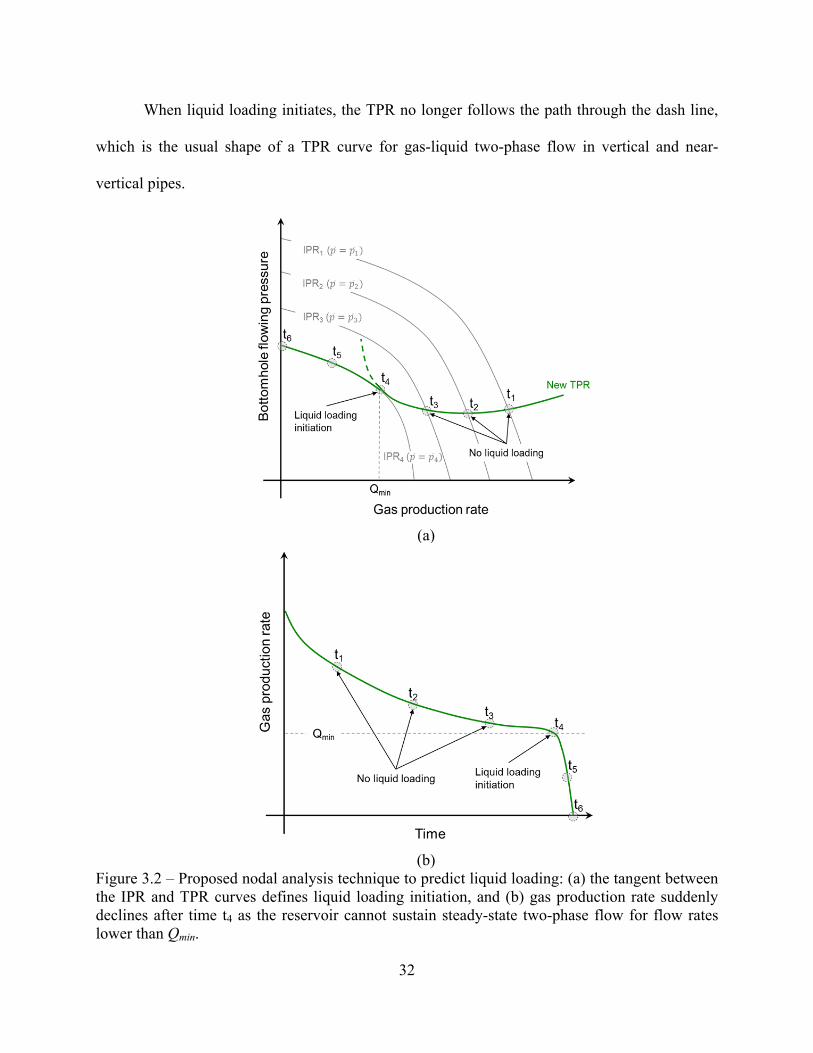
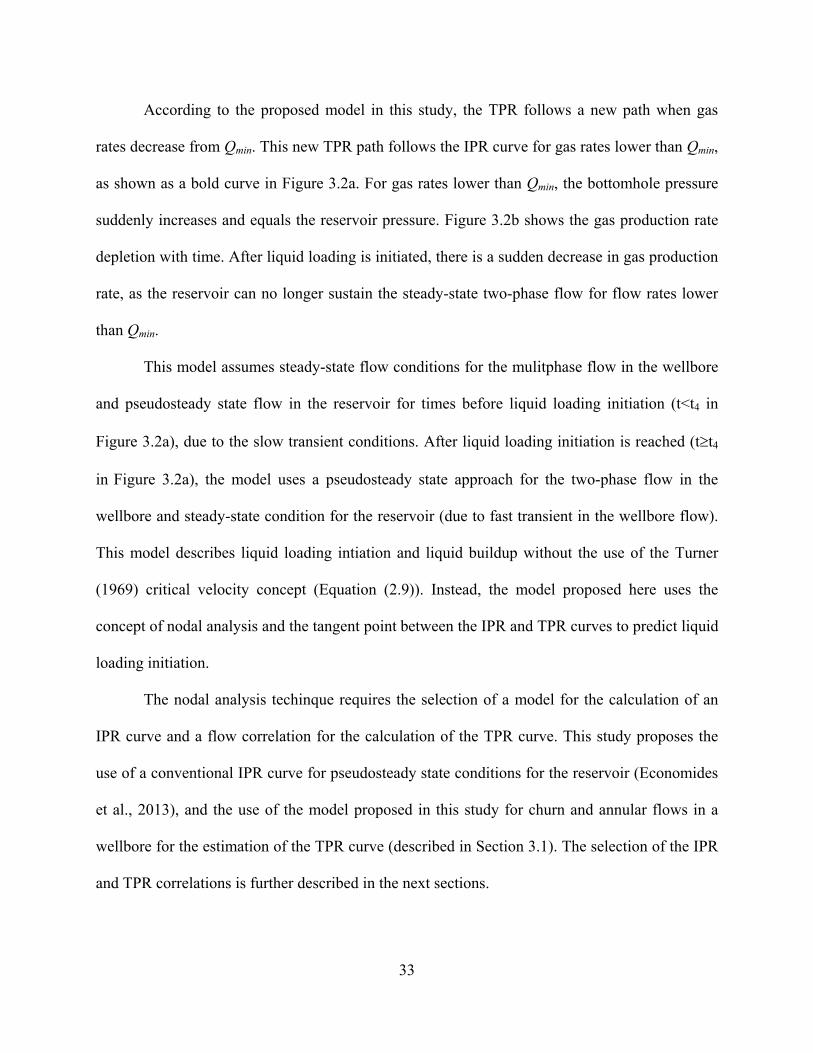
32

When liquid loading initiates, the TPR no longer follows the path through the dash line,

which is the usual shape of a TPR curve for gas-liquid two-phase flow in vertical and near-

vertical pipes.

(a)

(b)

Figure 3.2 – Proposed nodal analysis technique to predict liquid loading: (a) the tangent between the IPR and TPR curves defines liquid loading initiation, and (b) gas production rate suddenly declines after time t4 as the reservoir cannot sustain steady-state two-phase flow for flow rates lower than Qmin.

33

According to the proposed model in this study, the TPR follows a new path when gas

rates decrease from Qmin. This new TPR path follows the IPR curve for gas rates lower than Qmin,

as shown as a bold curve in Figure 3.2a. For gas rates lower than Qmin, the bottomhole pressure

suddenly increases and equals the reservoir pressure. Figure 3.2b shows the gas production rate

depletion with time. After liquid loading is initiated, there is a sudden decrease in gas production

rate, as the reservoir can no longer sustain the steady-state two-phase flow for flow rates lower

than Qmin.

This model assumes steady-state flow conditions for the mulitphase flow in the wellbore

and pseudosteady state flow in the reservoir for times before liquid loading initiation (t<t4 in

Figure 3.2a), due to the slow transient conditions. After liquid loading initiation is reached (tt4

in Figure 3.2a), the model uses a pseudosteady state approach for the two-phase flow in the

wellbore and steady-state condition for the reservoir (due to fast transient in the wellbore flow).

This model describes liquid loading intiation and liquid buildup without the use of the Turner

(1969) critical velocity concept (Equation (2.9)). Instead, the model proposed here uses the

concept of nodal analysis and the tangent point between the IPR and TPR curves to predict liquid

loading initiation.

The nodal analysis techinque requires the selection of a model for the calculation of an

IPR curve and a flow correlation for the calculation of the TPR curve. This study proposes the

use of a conventional IPR curve for pseudosteady state conditions for the reservoir (Economides

et al., 2013), and the use of the model proposed in this study for churn and annular flows in a

wellbore for the estimation of the TPR curve (described in Section 3.1). The selection of the IPR

and TPR correlations is further described in the next sections.

34

3.2.1 Reservoir Inflow Performance Model (IPR)

The reservoir model uses conventional gas inflow performance relationships. As liquid

loading occurs in the late life of gas wells, pseudosteady state conditions can be assumed and

non-Darcy effects can be neglected. Therefore, the IPR for the gas reservoir is calculated by the

following expression:

(3.21)

where qg is the production gas flow rate, J is the productivity index, is the average reservoir

pressure, pwf is the wellbore bottomhole flowing pressure.

To capture the transient decline in the gas flow rate, pseudosteady state change in the

average reservoir pressure ( ) can be obtained using reservoir material balance (Economides et

al., 2013). A simple version of gas material balance is given by the following well-known

expression,

1 (3.22)

where is the reservoir pressure, z is the gas compressibility factor, Gp is the cumulative

production, and Gi is the initial gas-in-place. The subscript i means initial, n refers to the current

time step, and the bar over the and the z means average conditions. Based on the knowledge of

the reservoir initial conditions, and on the current pressure and gas compressibility, npG is

calculated for each time step ∆ , assuming production gas flow rate constant within each time

step.

3.2.2 Tubing Performance Relationship (TPR)

The Gray (1974) correlation is the most widely used flow correlation to calculate

pressure drop over the tubing for gas wells. This correlation was shown to predict pressure drop

35

accurately over a wide range of conditons in gas wells (Reinicke et al., 1987). However, as

shown by Oudeman (1990), the Gray correlation may present problems for low-pressure, low-

gas rate wells. Oudeman showed an example where the Gray correlation underpredicted the

actual pressure gradient by 27%, for a low-gas rate well. As liquid loading occurs in the late life

of gas wellsit is important to develop and test improved models for low-pressure, low-rate wells.

This study uses the new wellbore model proposed in this study (see Section 3.1), which is

based on a mechanistic model for gas-liquid annular and churn flow regimes. This model is

described in Section 3.1, and it is validated with laboratory and field data over a wide range of

conditions, including low pressure low gas rate flows. This validation is presented and discussed

in Section 4.1. The accuracy of the model described in Section 3.1 for prediction of pressure

gradient was compared to measured data using natural gas-oil and air-water mixtures, for pipe

diameters ranging from 0.032 m (1.25 in) to 0.28 m (11 in), and pressures from 1 bara (15 psia)

to 614 bara (8,900 psia). When using field data, the absolute average errors for the TPR model

presented in this study (Section 4.1) on the prediction of bottomhole pressure, and pressure

profile along the wellbore, stayed within the range of 6%. More importantly, this TPR model

showed a superior accuracy in prediction of the laboratory measured pressure drop with varying

gas flow rate when compared to other widely used models for TPR estimation. Section 4.2 shows

that even though some TPR models show high accuracy for a wide range of conditions, if the

same models have inferior accuracy for low gas rates (for instance, the case of the Gray (1974)

correlation), they may not be desirable for prediction of liquid loading in gas wells.

After the selection of the correlations for the IPR and TPR simulations, the nodal analysis

can be performed in order to find the liquid loading critical rate (Qmin). Once Qmin is reached,

(time t4 in Figure 3.2a), a sudden decrease in gas flow rate leads the liquid film to start falling,

36

which buildups in the bottom of the wellbore. This phenomenon represents pseudosteady state

changes in the fluid flow in the vertical or near-vertical tube. The study of Waltrich et al. (2015a)

shows experimentally that a new steady-state flow condition can be re-established in the

wellbore by a larger liquid holdup front flowing upwards from the bottom to the top of the tube,

if there is continuously liquid-and-gas injection from the reservoir.

The bottomhole pressure for times after t4 is calculated using a similar approach as

proposed by Dousi et al. (2006). The changes in the friction component (left term of the right

hand-side of Equations (3.1) and (3.2)) are neglected since the gravitational effects at this point

are much larger than the frictional effects (due to the low-gas rates). Thus, only the increase in

bottomhole pressure due to the increase in the liquid column (hydrostatic pressure) is considered.

Then, the transient bottomhole flowing pressure for gas flow rates lower than Qmin (t5) is

calculated using the following expression,

, , (3.23)

where , is the bottomhole flowing pressure at a time , and , is the bottomhole

flowing pressure at liquid loading initiation (at time ), is the constant liquid rate inflow, A is

the cross-sectional area of the pipe, and is any time after liquid loading initiation, but before

the well stops flowing completely (time ).

The gas production keeps decreasing as the bottomhole pressure increases until it reaches

the average reservoir pressure (t6 in Figure 3.2a), when the well ceases production. In order to

calculate the time the wellbore stops flowing after it starts suffering from liquid loading,

Equation (3.24) is used, which is the rearrangement of Equation (3.23) replacing by :

, , (3.24)

37

where , is the bottomhole flowing pressure when well stop flowing, at time . This is the

pressure when gas production rate is zero, which is the same pressure as the given reservoir

pressure when the tangent of the IPR curve is the same as the TPR curve (see Figure 3.2a).

Liquid holdup from time up to time (right before liquid loading initiation) is usually

estimated from the solution of Equations (3.1) and (3.2). After time , this study proposes that

the liquid holdup at time ( , ) can be calculated by

, , (3.25)

where , is the liquid holdup at the time of liquid loading initiation, MD is the wellbore

measured depth, and is any time after liquid loading initiation (it can be replaced by or ).

Once the well stops flowing, tubing wellhead pressure increases, and the liquid column in

the bottom of the wellbore starts to be injected back into the formation (Dousi et al., 2006). A

new production cycle is re-started when the liquid holdup in the wellbore reaches the same level

at liquid loading initiation and wellhead pressure is lowered, assuming a continuous liquid

injection from the reservoir to the wellbore.

38

4. Model Validation, Results and Discussions 1, 2

This chapter is divided into two main sections. The first section shows the validation of

the model proposed in this study for churn and annular flow regimes, using laboratory and field

data. Simulations using PIPESIM software (PIPESIM, 2013) for different correlations are also

presented. All the simulations were performed for each data point of the experimental and field

data selected for this study. The second section of this chapter discusses the validation and

results on the prediction of liquid loading initiation based on a set of field data for 10 wells. It

also compares the prediction of liquid loading initiation using the current models available in the

literature (as described in Section 2.2).

Churn and Annular Flow Modeling Validation Results 4.1

The accuracy of the proposed model is compared with laboratory data (using databases

from Owen, 1986; Van der Meulen, 2012; Yuan et al., 2013; Zabaras et al., 2013; Skopich et al.,

2015), and field data (using the data set from Fancher and Brown, 1963; Reinicke et al., 1987).

The data collected from these different studies includes a wide range of pipe diameters of 0.0318

to 0.2794 m (1.252 to 11 in) and pressures of 1 to 613 bara (15 to 8,900 psia), in both air-water

and oil-natural gas systems. Also, different correlations found in the PIPESIM software

(PIPESIM, 2013), as well as in the previous model of Jayanti and Brauner (1994), were used to

simulate this set of data and to compare their performance against the model proposed in this

study.

1Section 4.1 of this chapter previously appeared as E. Pagan, W. C. Williams, S. Kam, P. J. Waltrich, Modeling Vertical Flow in Churn and Annular Flow Regimes in Small- and Large-Diameter Pipes, Paper Presented and Published at BHR Group’s 10th North American Conference on Multiphase Technology 8-10th June 2016. It is reprinted by permission of Copyright © 2016 BHR Group. See Appendix for more details. 2Section 4.2 of this chapter previously appeared as Erika V. Pagan, Wesley Williams, and Paulo J. Waltrich, A Simplified Transient Model to Predict Liquid Loading in Gas Wells, Paper SPE-180403-MS presented at the SPE Western Regional Meeting held in Anchorage, Alaska, USA, 23-26 May 2016. It is reprinted by permission of Copyright 2016, Society of Petroleum Engineers Inc. Copyright 2016, SPE. Reproduced with permission of SPE. Further reproduction prohibited without permission. See Appendix for more details.

39

4.1.1 Comparison with Laboratorial Data

A literature search identified five laboratory data sets including experimental data with

pipe diameters ranging from 0.032 m (1.25 in) to 0.279 m (11 in), using air-water mixtures at the

conditions close to the atmospheric pressure.

Figure 4.1 and Figure 4.2 present the comparison between simulation results from the

model in this study and experimental data obtained by Skopich et al. (2015) in vertical pipes of

diameters 0.0508 m (2 in) and 0.1016 m (4 in). The modeling results of Ansari et al. (1994) and

OLGA (2000) are also provided by Skopich et al. (2015). In this study, simulation results using

Duns and Ros (1963), Gray (1974), and Jayanti and Brauner (1994) models are added. Since

Jayanti and Brauner (1994) method was proposed only for churn flow regime, the simulation

results are not included for this model for flow regimes different than churn flow.

Figure 4.1 presents the pressure gradient and liquid holdup at the diameter of 0.0508 m (2

in), and superficial liquid velocities of 0.01 and 0.05 m/s. The model in this study predicts

annular flow at superficial gas velocities higher than 20 m/s, and churn flow regime for lower

gas velocities. This flow regime transition shows a reasonable agreement with the experimental

flow regime transition observations of Skopich et al. (2015). Figure 4.1 shows that the model

proposed in this study also has a good agreement in terms of pressure gradient at pipe diameter

of 0.0508 m (2 in), for both superficial liquid velocities, and for the wide range of superficial gas

velocities tested. Since this study is based on Jayanti and Brauner (1994) model, it is not

surprising that both models present similar results for churn flow and small diameter conditions,

as the models from the latter authors was originally developed for small diameter pipes. The

other models (with exception of Duns and Ros (1963) model) showed a good prediction of

pressure gradient only for annular flow, but seem to fail to capture the trend for churn flow (e.g.,

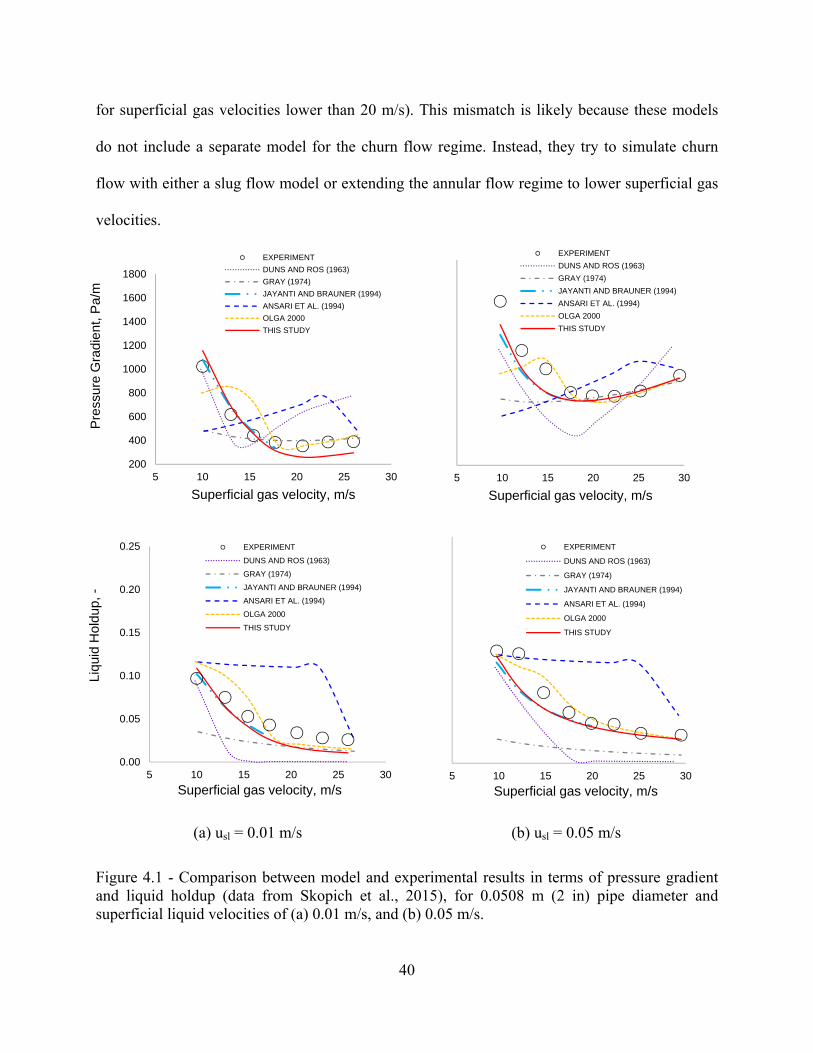
40

for superficial gas velocities lower than 20 m/s). This mismatch is likely because these models

do not include a separate model for the churn flow regime. Instead, they try to simulate churn

flow with either a slug flow model or extending the annular flow regime to lower superficial gas

velocities.

(a) usl = 0.01 m/s (b) usl = 0.05 m/s

Figure 4.1 - Comparison between model and experimental results in terms of pressure gradient and liquid holdup (data from Skopich et al., 2015), for 0.0508 m (2 in) pipe diameter and superficial liquid velocities of (a) 0.01 m/s, and (b) 0.05 m/s.

200

400

600

800

1000

1200

1400

1600

1800

5 10 15 20 25 30

Pre

ssur

e G

radi

ent,

Pa/

m

Superficial gas velocity, m/s

EXPERIMENT

DUNS AND ROS (1963)

GRAY (1974)

JAYANTI AND BRAUNER (1994)

ANSARI ET AL. (1994)

OLGA 2000

THIS STUDY

5 10 15 20 25 30

Superficial gas velocity, m/s

EXPERIMENT

DUNS AND ROS (1963)

GRAY (1974)

JAYANTI AND BRAUNER (1994)

ANSARI ET AL. (1994)

OLGA 2000

THIS STUDY

0.00

0.05

0.10

0.15

0.20

0.25

5 10 15 20 25 30

Liqu

id H

oldu

p, -

Superficial gas velocity, m/s

EXPERIMENT

DUNS AND ROS (1963)

GRAY (1974)

JAYANTI AND BRAUNER (1994)

ANSARI ET AL. (1994)

OLGA 2000

THIS STUDY

5 10 15 20 25 30

Superficial gas velocity, m/s

EXPERIMENT

DUNS AND ROS (1963)

GRAY (1974)

JAYANTI AND BRAUNER (1994)

ANSARI ET AL. (1994)

OLGA 2000

THIS STUDY

41

In the other hand, Duns and Ros (1963) correlation have a different result, presenting

reasonable predictions for churn regime, however, over predicting pressure gradient for annular

flow conditions.

Figure 4.1 also shows the experimental liquid holdup obtained by Skopich et al. (2015)

for a 0.0508 m (2 in) pipe diameter. Overall the model proposed in this study exhibits a better

performance in terms of liquid holdup prediction. The model proposed in this study, Jayanti and

Brauner (1994), and OLGA (2000) are the only models predicting the trends and magnitudes of

liquid holdup for all the entire range of superficial gas velocities. The model of Duns and Ros

(1963) shows a reasonable match for low superficial velocities, under predicting values of

holdup when increasing superficial gas velocities. Jayanti and Brauner (1994) correlation shows

similar results to this study for churn flow regime. Simulation results for annular flow regime is

not included for Jayanti and Brauner (1994), as the original work of these authors do not include

a separate model for annular flow.

For intermediate pipe diameters, the model in this study also shows a reasonable

performance. Figure 4.2 presents the experimental pressure gradient and liquid holdup for a pipe

diameter of 0.1016 m (4 in). The model proposed in this study shows an acceptable prediction of

the experimental pressure gradient values and trend for the entire range of superficial gas

velocities tested. The simulation results from Jayanti and Brauner (1994) for larger diameter

show over predictions for the experimental pressure gradient when compared to the model

proposed in this study. From Figure 4.2, it is possible to note that this study improved the model

of Jayanti and Brauner (1994) for churn flow regime, decreasing the over prediction of pressure

gradient for intermediate pipe diameters. Duns and Ros (1963), Gray (1974), Ansari et al.

(1994), OLGA (2000), and the model in this study show a good agreement for the annular flow

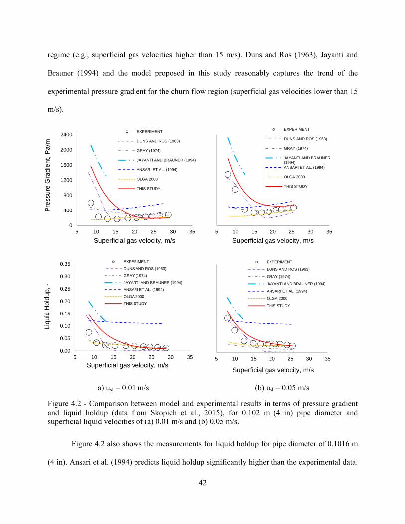
42

regime (e.g., superficial gas velocities higher than 15 m/s). Duns and Ros (1963), Jayanti and

Brauner (1994) and the model proposed in this study reasonably captures the trend of the

experimental pressure gradient for the churn flow region (superficial gas velocities lower than 15

m/s).

a) usl = 0.01 m/s (b) usl = 0.05 m/s

Figure 4.2 - Comparison between model and experimental results in terms of pressure gradient and liquid holdup (data from Skopich et al., 2015), for 0.102 m (4 in) pipe diameter and superficial liquid velocities of (a) 0.01 m/s and (b) 0.05 m/s.

Figure 4.2 also shows the measurements for liquid holdup for pipe diameter of 0.1016 m

(4 in). Ansari et al. (1994) predicts liquid holdup significantly higher than the experimental data.

0

400

800

1200

1600

2000

2400

5 10 15 20 25 30 35

Pre

ssur

e G

radi

ent,

Pa/

m

Superficial gas velocity, m/s

EXPERIMENT

DUNS AND ROS (1963)

GRAY (1974)

JAYANTI AND BRAUNER (1994)

ANSARI ET AL. (1994)

OLGA 2000

THIS STUDY

5 10 15 20 25 30 35

Superficial gas velocity, m/s

EXPERIMENT

DUNS AND ROS (1963)

GRAY (1974)

JAYANTI AND BRAUNER(1994)ANSARI ET AL. (1994)

OLGA 2000

THIS STUDY

0.00

0.05

0.10

0.15

0.20

0.25

0.30

0.35

5 10 15 20 25 30 35

Liqu

id H

oldu

p, -

Superficial gas velocity, m/s

EXPERIMENT

DUNS AND ROS (1963)

GRAY (1974)

JAYANTI AND BRAUNER (1994)

ANSARI ET AL. (1994)

OLGA 2000

THIS STUDY

5 10 15 20 25 30 35

Superficial gas velocity, m/s

EXPERIMENT

DUNS AND ROS (1963)

GRAY (1974)

JAYANTI AND BRAUNER (1994)

ANSARI ET AL. (1994)

OLGA 2000

THIS STUDY

43

All the other models showed accuracy to the liquid holdup prediction similar to the results for

pressure gradient.

Figure 4.3 presents the experimental pressure gradient for a 0.127 m (5 in) pipe diameter.

The model proposed in this study again shows a good prediction of experimentally measured

pressure gradient values and trend. Overall it shows a better performance when compared to the

other models tested for matching the experimental pressure gradient data for both superficial

liquid velocities. For both superficial liquid velocities presented in Figure 4.3, churn flow regime

was predicted to happen from low superficial gas velocities up to 9 m/s, when the flow regime

changed to annular.

(a) usl = 0.02 m/s (b) usl = 0.7 m/s

Figure 4.3 - Comparison between model and experimental results in terms of pressure gradient (data from Van de Meulen, 2012), for 0.127 m (5 in) pipe ID, and liquid superficial velocities of (a) 0.02 m/s and (b) 0.7 m/s.

For larger pipe diameters, the model proposed in this study also shows good

performance. Figure 4.4 presents the experimentally measured pressure gradient for a 0.2794 m

(11 in) pipe diameter. Again, the model proposed in this study shows a good prediction of

pressure gradient for the entire range of superficial gas velocities. All the experimental values

0

1000

2000

3000

4000

5000

2 4 6 8 10 12 14

Pre

ssur

e gr

adie

nt, P

a/m

Superficial gas velocity, m/s

EXPERIMENTDUNS AND ROS (1963)GRAY (1974)JAYANTI AND BRAUNER (1994)ANSARI ET AL. (1994)OLGA 2000THIS STUDY

2 4 6 8 10 12 14Superficial gas velocity, m/s

EXPERIMENTDUNS AND ROS (1963)GRAY (1974)JAYANTI AND BRAUNER (1994)ANSARI ET AL. (1994)OLGA 2000THIS STUDY

44

presented in the two graphs of Figure 4.4 are estimated to be in churn flow regime, according to

the correlations for flow regimes transition used in this study.

Figure 4.5 shows the comparison between experimental and calculated results for all

models evaluated in this study on the prediction of the experimental pressure gradient. Figure

4.5a includes the comparison for all the values of pressure gradient (354 data points), for five

different data sets previously published and collected for this study (Owen, 1986; Van der

Meulen, 2012; Yuan et al., 2013; Zabaras et al., 2013; Skopich et al., 2015).

(a) usl = 0.1 m/s (b) usl = 0.15 m/s

Figure 4.4 - Comparison between model and experiments results in terms of pressure gradient (data from Zabaras et al., 2013) for 0.279 m (11 in) pipe ID, and liquid superficial velocities of (a) 0.03 m/s and (b) 0.15 m/s.

Figure 4.5 shows that this study has an overall better performance when estimating the

pressure gradient for the experimental data when compared to the other flow models tested,

presenting an absolute average error of 36%. The best performance is followed by the results of

Gray (1974) correlation, OLGA (2000), Ansari et al. (1994) model, Duns and Ros (1963), and

Jayanti and Brauner (1994) method. Gray’s (1974) absolute average error is close to the error for

the model proposed in this study. However, this study captures the trend of the pressure gradient

0

2000

4000

6000

8000

2 4 6 8 10 12 14 16 18

Pre

ssur

e gr

adie

nt ,

Pa/

m

Superficial gas velocity, m/s

EXPERIMENT

DUNS AND ROS (1963)

GRAY (1974)

JAYANTI AND BRAUNER (1994)

ANSARI ET AL. (1994)

OLGA 2000

THIS STUDY

2 4 6 8 10 12 14 16 18

Superficial gas velocity, m/s

EXPERIMENT

DUNS AND ROS (1963)

GRAY (1974)

ANSARI ET AL. (1994)

JAYANTI AND BRAUNER (1994)

OLGA 2000

THIS STUDY

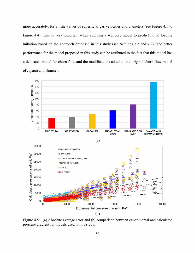
45

more accurately, for all the values of superficial gas velocities and diameters (see Figure 4.1 to

Figure 4.4). This is very important when applying a wellbore model to predict liquid loading

initiation based on the approach proposed in this study (see Sections 3.2 and 4.2). The better

performance for the model proposed in this study can be attributed to the fact that this model has

a dedicated model for churn flow and the modifications added to the original churn flow model

of Jayanti and Brauner.

(a)

(b)

Figure 4.5 – (a) Absolute average error and (b) comparison between experimental and calculated pressure gradient for models used in this study.

0

20

40

60

80

100

120

140

160

THIS STUDY GRAY (1974) OLGA 2000 ANSARI ET AL.(1994)

DUNS AND ROS(1963)

JAYANTI ANDBRAUNER (1994)

Abs

olut

e av

erag

e er

ror,

%

0

5000

10000

15000

20000

25000

30000

35000

0 2000 4000 6000 8000 10000

Cal

cula

ted

pres

sure

gra

dien

t, P

a/m

Experimental pressure gradient, Pa/m

DUNS AND ROS (1963)

GRAY (1974)

JAYANTI AND BRAUNER (1994)

ANSARI ET AL. (1994)

OLGA 2000

THIS STUDY

+ 20%‐ 20%

+ 50%

‐ 50%

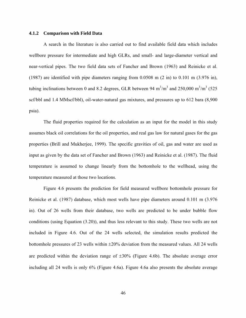
46

4.1.2 Comparison with Field Data

A search in the literature is also carried out to find available field data which includes

wellbore pressure for intermediate and high GLRs, and small- and large-diameter vertical and

near-vertical pipes. The two field data sets of Fancher and Brown (1963) and Reinicke et al.

(1987) are identified with pipe diameters ranging from 0.0508 m (2 in) to 0.101 m (3.976 in),

tubing inclinations between 0 and 8.2 degrees, GLR between 94 m3/m3 and 250,000 m3/m3 (525

scf/bbl and 1.4 MMscf/bbl), oil-water-natural gas mixtures, and pressures up to 612 bara (8,900

psia).

The fluid properties required for the calculation as an input for the model in this study

assumes black oil correlations for the oil properties, and real gas law for natural gases for the gas

properties (Brill and Mukherjee, 1999). The specific gravities of oil, gas and water are used as

input as given by the data set of Fancher and Brown (1963) and Reinicke et al. (1987). The fluid

temperature is assumed to change linearly from the bottomhole to the wellhead, using the

temperature measured at those two locations.

Figure 4.6 presents the prediction for field measured wellbore bottomhole pressure for

Reinicke et al. (1987) database, which most wells have pipe diameters around 0.101 m (3.976

in). Out of 26 wells from their database, two wells are predicted to be under bubble flow

conditions (using Equation (3.20)), and thus less relevant to this study. These two wells are not

included in Figure 4.6. Out of the 24 wells selected, the simulation results predicted the

bottomhole pressures of 23 wells within 20% deviation from the measured values. All 24 wells

are predicted within the deviation range of 30% (Figure 4.6b). The absolute average error

including all 24 wells is only 6% (Figure 4.6a). Figure 4.6a also presents the absolute average

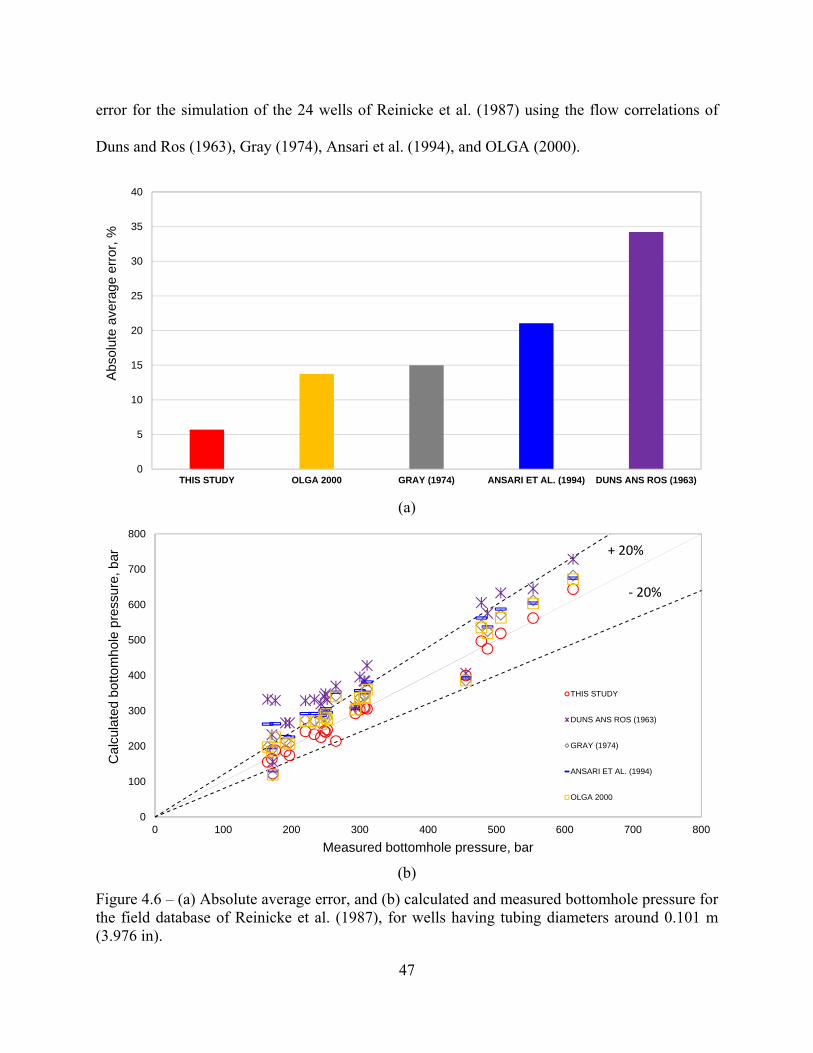
47

error for the simulation of the 24 wells of Reinicke et al. (1987) using the flow correlations of

Duns and Ros (1963), Gray (1974), Ansari et al. (1994), and OLGA (2000).

(a)

(b)

Figure 4.6 – (a) Absolute average error, and (b) calculated and measured bottomhole pressure for the field database of Reinicke et al. (1987), for wells having tubing diameters around 0.101 m (3.976 in).

0

5

10

15

20

25

30

35

40

THIS STUDY OLGA 2000 GRAY (1974) ANSARI ET AL. (1994) DUNS ANS ROS (1963)

Abs

olut

e av

erag

e er

ror,

%

0

100

200

300

400

500

600

700

800

0 100 200 300 400 500 600 700 800

Cal

cula

ted

botto

mho

le p

ress

ure,

bar

Measured bottomhole pressure, bar

THIS STUDY

DUNS ANS ROS (1963)

GRAY (1974)

ANSARI ET AL. (1994)

OLGA 2000

‐ 20%

+ 20%

48

The model proposed in this study resulted in an absolute average error much lower than

the other correlations tested. The model of Jayanti and Brauner (1994) was not used to simulate

this field data set since the wells were not only flowing under churn flow regime. It is clear to

conclude from Figure 4.6 that the model proposed in this study has significantly more accurate

for churn and annular flow in wellbore or larger diameter, when compared to the other widely

used models.

Figure 4.7 shows the comparison between the model and field data of Fancher and Brown

(1963) for pressure profile along the wellbore, and for smaller tubing diameters (0.05 m – or 2

in). In addition, it also shows the flow regimes as predicted by the model proposed in this study.

Figure 4.7 shows that the model proposed here has an excellent agreement with pressure profile

for the field data of Fancher and Brown (1963). This database includes 20 cases for different oil

rates and GLR. Twelve cases are selected from their database because they are predicted to have

churn or annular flow regimes (as predicted by the model) at least in a certain portion of the

wellbore.

Interestingly, the model proposed in this study predicts, with reasonable accuracy, the

pressure gradient for slug flow conditions, even though it was originally developed only for

churn and annular flow regimes. These results indicate that the model proposed in this study

should potentially be used to estimate slug flow in conditions near to the churn flow regime.

However, further investigations should be carried out before this statement can be confirmed.

Figure 4.8a presents the absolute average error for the simulation of the 12 wells of

Fancher and Brown (1963) using the model proposed in this study, as well as the correlations of

Duns and Ros (1963), Gray (1974), Ansari et al. (1994), and OLGA (2000).

49

Figure 4.7 - Comparison between simulation results using the model proposed in this study and measured wellbore pressure profile (field data from Fancher and Brown, 1963). Circles represent the measured pressures and continuous lines are the simulated pressures. Dash lines represents the depth at which a flow regime transition happened based on the simulation.

0

4

8

12

16

20

24

280 200 400 600 800 1000

Dep

th,

ft. x

102

Q = 144 BBL/DGLR = 7283 SCF/BBL

Field dataThis study

annular

0 200 400 600 800 1000

,

Q = 75 BBL/DGLR = 4900 SCF/BBL

churn

slug

0 200 400 600 800 1000

Depth, ft. x 10

Q = 144 BBL/DGLR = 3525 SCF/BBL

churn

slug

0

4

8

12

16

20

24

280 200 400 600 800 1000

Dep

th,

ft. x

102

Q = 312 BBL/DGLR = 2215 SCF/BBL

0 200 400 600 800

Q = 336 BBL/DGLR = 2180 SCF/BBL

churn

slug

annular

0 200 400 600 800 1000

DEP

TH, FT. x 102

Q = 144 BBL/DGLR = 1541

churn

slug

0

4

8

12

16

20

24

280 200 400 600 800 1000

Dep

th,

ft. x

102

Q = 696 BBL/DGLR = 1195 SCF/BBL

churn

slug

annular

0 200 400 600 800 1000

Q = 600 BBL/DG/L = 1056 SCF/BBL

slug

churn

0 200 400 600 800 1000

Q = 192 BBL/DGLR = 1035 SCF/BBL

churn

slug

0

4

8

12

16

20

24

280 200 400 600 800 1000

Dep

th,

ft. x

102

Pressure, psi

Q = 792BBL/DGLR = 890 SCF/BBL

slug

churn

0 200 400 600 800 1000

Pressure, psi

Q = 696 BBL/DGLR = 643 SCF/BBL

slug

churn

0 200 400 600 800 1000

Pressure, psi

Q = 936 BBL/DGLR = 525 SCF/BBL

slug

churn

slug 

churn 

annular 

50

Figure 4.8a shows that the absolute average error for the estimated pressure using the

model proposed in this study for all the 12 wells was only 5%.

(a)

(b)

Figure 4.8 - (a) Absolute average error, and (b) calculated and measured bottomhole pressure for the field database of Fancher and Brown (1963), for wells having tubing diameters around 0.0508 m (2 in).

0

2

4

6

8

10

12

OLGA 2000 GRAY (1974) THIS STUDY DUNS AND ROS(1963)

ANSARI ET AL.(1994)

Abs

olut

e av

erag

e er

ror,

%

0

100

200

300

400

500

600

700

800

0 100 200 300 400 500 600 700 800

Bot

tom

hole

Pre

ssur

e C

alcu

late

d, b

ar

Bottomhole Pressure Measured, bar

THIS STUDY

DUNS AND ROS (1963)

GRAY (1974)

ANSARI ET AL. (1994)

OLGA 2000

+ 20%

‐ 20%

51

OLGA (2000) presented the overall best estimation for the data set of Fancher and Brown

(1963), but its accuracy is essentially the same as the model proposed in this study. Ansari et al.

(1994) and Duns and Ros (1963) present larger errors compared to the other models.

Nevertheless, all flow model tested presented an absolute average error under 20% for this

database with smaller tubing diameters. The model of Jayanti and Brauner (1994) was not used

to simulate this field data set since the fluids in these wells were not only flowing in churn flow

regime.

Liquid Loading Modeling Validation and Result Discussions 4.2

There are a few field data sets available in the open literature regarding liquid loading in

gas wells. To the knowledge of the author, the most cited data sets are presented in Turner et al.

(1969), Coleman et al. (1991), and Veeken et al. (2010). However, from these three widely used

field data sets for liquid loading, the only one that includes enough information about wellbore

and reservoir is the data set of Veeken et al. (2010). More importantly, the latter authors describe

in details on how they have defined wells under liquid loading conditions. These authors have

defined the minimum flow rate (critical rate) just before the well ceases production, as shown in

Figure 4.9.

As liquid loading is a “field term” and can be interpreted differently by different engineers,

it is very important to clearly define liquid loading conditions for an appropriate validation of the

model. In addition to that, Veeken et al. (2010) also stated that they have only considered wells

with acceptable quality flow measurement (±20%). However, one of the drawbacks of the data

set published by Veeken et al. (2010) is the non-disclosure of the production data for condensate

or water flow rates. As liquid rates are usually low for gas wells, a fix water rate of 7.9 m3/D (50

bbl/D) is assumed here for all wells in Veeken et al. (2010) database. This value of condensate or

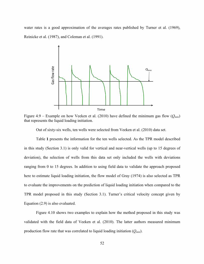
52

water rates is a good approximation of the averages rates published by Turner et al. (1969),

Reinicke et al. (1987), and Coleman et al. (1991).

Figure 4.9 – Example on how Veeken et al. (2010) have defined the minimum gas flow (Qmin) that represents the liquid loading initiation.

Out of sixty-six wells, ten wells were selected from Veeken et al. (2010) data set.

Table 1 presents the information for the ten wells selected. As the TPR model described

in this study (Section 3.1) is only valid for vertical and near-vertical wells (up to 15 degrees of

deviation), the selection of wells from this data set only included the wells with deviations

ranging from 0 to 15 degrees. In addition to using field data to validate the approach proposed

here to estimate liquid loading initiation, the flow model of Gray (1974) is also selected as TPR

to evaluate the improvements on the prediction of liquid loading initiation when compared to the

TPR model proposed in this study (Section 3.1). Turner’s critical velocity concept given by

Equation (2.9) is also evaluated.

Figure 4.10 shows two examples to explain how the method proposed in this study was

validated with the field data of Veeken et al. (2010). The latter authors measured minimum

production flow rate that was correlated to liquid loading initiation (Qmin).

53

Table 1 – Liquid loading data set for vertical and near-vertical gas wells published by Veeken et al. (2010).

Wellbore geometry Reservoir and fluid properties

Production data

Wellhead Bottomhole

Well MD (m) TVD

(m)

ID

(in.)

Dev.

(deg.)

Gas SG

(-)

J

(e3Sm3/D/bar2)

Pressure

(bara)

Temperature

(oC)

Temperature

(oC)

Qmin

(Sm3/D)

5 2,000 2,000 2.99 90 0.59 0.091 6 16 52 26,000

27 4,120 4,120 4.28 90 0.59 0.019 98 50 158 200,000

28a 4,120 4,120 4.28 90 0.59 0.053 85 50 158 200,000

28b 4,120 4,120 4.28 90 0.59 0.077 50 73 158 170,000

29 4,120 4,120 4.28 90 0.59 0.060 85 50 158 180,000

7 2,060 2,000 2.87 76 0.59 0.091 5.5 16 52 24,000

21 3,445 3,350 4.41 77 0.63 0.035 15 62 115 100,000

29a 3,130 3,025 6.09 75 0.61 0.909 46 75 120 530,000

29b 3,130 3,025 6.09 75 0.61 0.909 34 69 120 390,000

52 2,660 2,570 6.09 75 0.65 0.455 91 53 80 737,000

54

(a)

(b)

Figure 4.10 – Examples on how the method of using IPR tangent to TPR curve was validated with the minimum production flow rate for wells: (a) 28a, (b) 28b in Veeken et al. (2010) database. The figure also shows the results for the prediction of liquid loading initiation using the droplet model of Turner et al. (1969).

The model proposed here calculated this minimum production rate using nodal analysis,

with different correlations to estimate the TPR curve (correlation proposed in this study and Gray

90

100

110

120

130

140

150

0 150,000 300,000 450,000 600,000 750,000 900,000

Bot

tom

hole

flow

ing

pres

sure

, bar

a

Production gas flow rate, Sm3/D

‐15% 

‐22%

This studyTurner

Gray (1974)

+13%ActualQmin

40

50

60

70

80

90

100

110

120

0 100,000 200,000 300,000 400,000 500,000 600,000

Bot

tom

hole

flow

ing

pres

sure

, bar

a

Production gas flow rate, Sm3/D

This study

Gray (1974)

‐21% 

Turner

‐34%

+9%

ActualQmin

55

(1974) correlation). Liquid loading was estimated to be initiated when the IPR curve was tangent

to the TPR curve.

The value of gas rate when the IPR is tangent to the TPR curve defines the minimum gas

rate (Qmin), which defines when the gas well starts suffering from liquid loading. Figure 4.10a

and b also present the estimation of the minimum gas rate calculated by the droplet model of

Turner et al. (1969). The results are shown in these figures in terms of percentage error from the

models estimation to the actual field data of liquid loading initiation (actual Qmin) as presented by

Veeken et al. (2010).

The model validation results for all ten wells are shown in Figure 4.11. From these

results, it is possible to conclude that the model proposed in this study using the TPR correlation

proposed in this study has an overall better performance than the flow correlation of Gray (1974)

and Turner critical flow rate.

It is important to point out the fact that the absolute average error for the proposed model

using the TPR correlation proposed in this study stayed within the range of +17%, which is

within the range of the accuracy of the flow measurements (20%) for the field data published

by Veeken et al. (2010). When using Gray (1974) correlation for the TPR curve, the average

error is slightly greater than 20%, which means that the concept of IPR tangent to the TPR curve

still works with a reasonable accuracy when using Gray correlation. However, the TPR

correlation proposed in this study has shown to be more accurate than Gray’s for low and high

gas rates. Larger deviations when using Gray (1974) correlation for low-pressure low-gas rates

are also observed on the studies of Waltrich et al. (2015b) and in this study (shown in Section

4.1) using laboratory and field data.

56

(a)

(b)

Figure 4.11 – (a) Relative error, and (b) absolute average error for the comparison between field data published by Veeken et al. (2010) for the predicted minimum flow rate for liquid loading initiation. These results show the prediction for the field data using the concept of IPR tangent to the TPR proposed, using TPR model proposed in this study and Gray (1974). Turner et al. (1969) critical flow rate is also compared to the same field data set. The angle () above the x-axis in figure (a) indicates the inclination of the well.

-80

-60

-40

-20

0

20

24,000 26,000 100,000 170,000 180,000 200,000 200,000 390,000 530,000 737,000

Rel

ativ

e E

rror

, %

Actual Qmin, m3/D

This study

Turner et al. (1969)

Gray (1974)

14o 0o 13o 15o0o 0o 0o 0o 15o15o

0

5

10

15

20

25

30

35

This study Gray (1974) Turner et al. (1969)

Abs

olut

e av

erag

e er

ror,

%

57

The droplet model of Turner et al. (1969) resulted in an average error of approximately

32%, which is significantly larger than the accuracy of the flow measurement of 20%. It is also

important to mention that for some wells in the data set of Veeken et al. (2010), Turner et al.

(1969) critical flow rate is lower than the minimum flow for the tangent point of intersection

between IPR and TPR.

If one assumes that the IPR and TPR curves are good physical representations of the fluid

flow behavior in the reservoir and wellbore (which is a widely accepted assumption), the

minimum flow rate predicted by the Turner (1969) correlation would be physically impossible,

as the minimum flow rate possible for a well is at the tangent between the IPR and TPR curves.

In other words, in order for the reservoir to deliver the fluids to the surface through the wellbore,

the IPR curve needs to intersect the TPR curve. At a gas flow rate lower than the tangent

between the IPR and TPR curves, the IPR and TPR can no longer cross each other, so flow from

reservoir to the surface through the wellbore is no longer possible.

Two other important features for the field data of Veeken et al. (2010), which makes the

validation in this study relevant are the wide range of productive index (J) and wellbore diameter

included in this database. As concluded by Riza et al. (2015) after a parametric study,

productivity index and wellbore diameter are the dominate parameters in the determination of

minimum flow rate for liquid loading initiation. Also, the same dataset features a wide range of

wellhead pressures, minimum flow rates, and well inclinations. Belfroid et al. (2008) suggested

that the Turner critical velocity should be modified to work appropriately on wells with

inclinations other than vertical. In fact, as it is shown in Figure 4.11a, Turner’s criterion have

higher relative errors for larger well inclinations, while the model in this study shows only an

58

average error around 20% for such wells, which is still within the data measurement uncertainty

of (20%).

4.2.1 Testing the Concept of Minimum Pressure Point and Nodal Analysis (Lea et al.,

2003) with Field Data of Veeken et al. (2010)

The approach of using the IPR tangent to the TPR curve is also compared to the concept

of minimum pressure as previously described by Lea et al. (2003) (see Section 3.2). For each

well, the TPR had already been calculated using the model proposed in this study and Gray

(1974) correlation. Thus, to estimate the liquid loading initiation using the concept of minimum

pressure, only one additional step to determine the lowest pressure value for each TPR is needed.

After these values are determined, the results for all the 10 wells are presented in Figure 4.12.

The results for the droplet model of Turner et al. (1969) are also included. From Figure

4.12a, it is possible to conclude that the error using the model for TPR proposed in this study

provides better results than the Gray (1974) correlation.

Figure 4.12b compares the concept of minimum pressure and the method of using IPR

tangent to the TPR curve. From this figure, it is clear to see that the concept of the IPR tangent to

the TPR curve provide better results than the minimum pressure method. When using the model

proposed in this study for the TPR, and the concept of IPR tangent to the TPR to predict liquid

loading initiation, the average error resulted in only 17%, while the average error was around

23% when using same concept but with the Gray (1974) correlation. The critical flow rate

criterion of Turner shows a superior prediction when compared to the minimum pressure concept

of Lea et al. (2003), but the Turner criterion has significantly larger errors when using the

method of IPR tangent to TPR, particularly when using the TPR based on the model proposed in

this study for churn and annular flow regimes.

59

(a)

(b)

Figure 4.12 – (a) Relative error and (b) absolute average error for the comparison between field data published by Veeken et al. (2010) for the predicted minimum flow rate for liquid loading initiation when using the concept of minimum pressure of Lea et al. (2003) with the TPR model proposed in this study and Gray (1974). Figure 4.12b also includes the results previously presented in Figure 4.11b. The results for Turner et al. (1969) critical flow rate are also compared. The angle () above the x-axis in figure (a) indicates the inclination of the well.

4.2.2 Explaining Liquid Loading Field Symptoms Using the Proposed Model

This section shows how to use the model proposed in this study for prediction of liquid

loading initiation to describe the field symptoms observed for a gas well under liquid loading

conditions.

-100

-75

-50

-25

0

25

50

75

100

24,000 26,000 100,000 170,000 180,000 200,000 200,000 390,000 530,000 737,000

Rel

ativ

e E

rror

, %

Actual Qmin, m3/D

This study

Turner et al. (1969)

Gray (1974)

14o 0o 13o 15o0o 0o 0o 0o 15o15o

0

5

10

15

20

25

30

35

40

45

50

This study Gray (1974) Turner et al. (1969)

Abs

olut

e av

erag

e er

ror,

%

IPR tangent to TPR

Minimum pressure

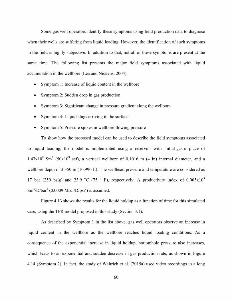
60

Some gas well operators identify these symptoms using field production data to diagnose

when their wells are suffering from liquid loading. However, the identification of such symptoms

in the field is highly subjective. In addition to that, not all of these symptoms are present at the

same time. The following list presents the major field symptoms associated with liquid

accumulation in the wellbore (Lea and Nickens, 2004):

Symptom 1: Increase of liquid content in the wellbore

Symptom 2: Sudden drop in gas production

Symptom 3: Significant change in pressure gradient along the wellbore

Symptom 4: Liquid slugs arriving in the surface

Symptom 5: Pressure spikes in wellbore flowing pressure

To show how the proposed model can be used to describe the field symptoms associated

to liquid loading, the model is implemented using a reservoir with initial-gas-in-place of

1.47x109 Sm3 (50x109 scf), a vertical wellbore of 0.1016 m (4 in) internal diameter, and a

wellbore depth of 3,350 m (10,990 ft). The wellhead pressure and temperature are considered as

17 bar (250 psig) and 23.9 oC (75 o F), respectively. A productivity index of 0.005x103

Sm3/D/bar2 (0.0009 Mscf/D/psi2) is assumed.

Figure 4.13 shows the results for the liquid holdup as a function of time for this simulated

case, using the TPR model proposed in this study (Section 3.1).

As described by Symptom 1 in the list above, gas well operators observe an increase in

liquid content in the wellbore as the wellbore reaches liquid loading conditions. As a

consequence of the exponential increase in liquid holdup, bottomhole pressure also increases,

which leads to an exponential and sudden decrease in gas production rate, as shown in Figure

4.14 (Symptom 2). In fact, the study of Waltrich et al. (2015a) used video recordings in a long

61

(42-m high) and transparent vertical tube to show that a sudden change in gas flow rate can lead

to liquid falling to the bottom of the tube.

Figure 4.13 – Simulated results shows the increase on wellbore liquid holdup over time using the proposed model with correlation for TPR proposed in this study. This increase in liquid content in the wellbore is often correlated in the field to liquid loading symptoms.

The latter authors also show that after a sudden change in gas flow rate, there is a

significant change in pressure gradient along the wellbore (Symptom 3), as a consequence of

larger liquid content in the bottom of the tube. However, the steady-state pressure gradient for

the new lower gas rate is slowly re-established as liquid flow upwards, as long as liquid and gas

injection rates are continued. The experiments of Waltrich et al. (2015a) also show that after this

sudden change in gas rate, there is a significant increase in the pressure oscillation along the tube

(Symptom 5), and it is possible to observe a high amount of liquid content flowing upward in the

tubing (Symptom 4). Furthermore, the experiments of Waltrich et al. (2015a) showed through

video recordings and simulation results that the liquid droplets are flowing upwards, for gas

velocities lower than the critical criterion of Turner et al. (1969). Thus, this study brings more

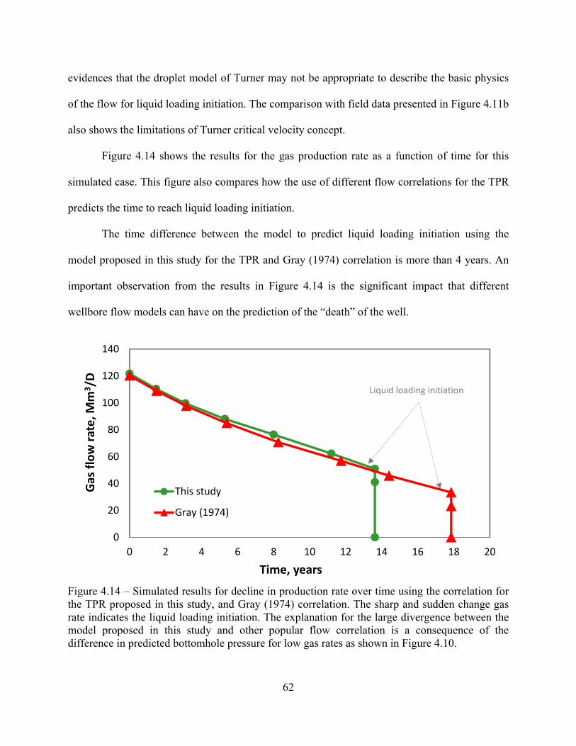
62

evidences that the droplet model of Turner may not be appropriate to describe the basic physics

of the flow for liquid loading initiation. The comparison with field data presented in Figure 4.11b

also shows the limitations of Turner critical velocity concept.

Figure 4.14 shows the results for the gas production rate as a function of time for this

simulated case. This figure also compares how the use of different flow correlations for the TPR

predicts the time to reach liquid loading initiation.

The time difference between the model to predict liquid loading initiation using the

model proposed in this study for the TPR and Gray (1974) correlation is more than 4 years. An

important observation from the results in Figure 4.14 is the significant impact that different

wellbore flow models can have on the prediction of the “death” of the well.

Figure 4.14 – Simulated results for decline in production rate over time using the correlation for the TPR proposed in this study, and Gray (1974) correlation. The sharp and sudden change gas rate indicates the liquid loading initiation. The explanation for the large divergence between the model proposed in this study and other popular flow correlation is a consequence of the difference in predicted bottomhole pressure for low gas rates as shown in Figure 4.10.

0

20

40

60

80

100

120

140

0 2 4 6 8 10 12 14 16 18 20

Gas flow rate, M

m3/D

Time, years

This study

Gray (1974)

Liquid loading initiation

63

Waltrich et al (2015b) have shown that widely-used wellbore flow correlations (such as

Gray, 1974) have a poor prediction for low-liquid, low-gas and low-pressure two-phase flows in

long vertical tubes. The use of model proposed in this study for flows under churn and annular

conditions (TPR model) has shown to be more accurate to predict liquid loading initiation (see

Figure 4.11) for a wide range of conditions. The model proposed in this study has shown that this

TPR model has a good prediction for low- and high-liquid, low- and high-gas and low- and high-

pressure two-phase flows in short and long vertical and near-vertical tubes with small and large

diameters (see model validation in Section 4.1).

As shown in Figure 4.10, both this study and Gray (1974) models have similar results for

the bottomhole pressure until close to the minimum point. However, for gas flow rates lower

than the minimum point, there is a significant discrepancy between these models. The main

reason for this difference is the inclusion of a more robust churn flow model in this study. Gray

(1974) correlation was not originally developed for low-pressure low-gas rate conditions, and it

may not give good predictions for these conditions, as stated previously in the study of Oudeman

(1990). The model proposed in this thesis was developed and validated for a wide range of pipe

diameters, pressure, and flow rates, including low-pressure low-gas low-liquid rate conditions.

The model proposed in this study assumes that the reservoir does not have enough

pressure at the bottom of the wellbore to sustain steady-state flow for gas flow rates lower than

Qmin. Once the pressure in the reservoir is not enough, gas production rate starts to decrease

suddenly, which consequently leads to liquid falling back to the bottom of the wellbore. The

results in Figure 4.14 show only one cycle for a well under liquid loading conditions. A new

cycle would start as the liquid is drained back to the formation as suggested by Dousi et al.

(2006). Once the wellbore liquid holdup drops below the amount of liquid at liquid loading

64

initiation, the gas production would re-start (assuming a constant wellhead pressure). The

metastable flow could be also modeled here as proposed by Dousi et al. (2006), but the focus on

this thesis is to show the liquid loading initiation using nodal analysis and abandonment pressure

concept rather than simulating metastable flows.

Figure 4.15 shows the results for the simulated case (using TPR proposed in this study –

Section 3.1) using a schematic representation in terms of production gas rate, (in Mscf/D),

liquid holdup, , and flow regimes at the different times in the life of the well.

Figure 4.15 – Schematic representation of the change in wellbore liquid holdup, for different times for the simulated case.

This schematic representation presents how the gas-liquid flow behaves inside the

wellbore from time to . The arrows represent the flowing direction of the fluids. At times

and both liquid and gas phases flow in the upward direction. During this period of time, the

65

fluids are flowing with an annular flow regime (upward thin wall liquid film and a gas core with

a few entrained droplets). Reservoir pressure keeps decreasing with time, and so, gas production

rate also decreases. As a consequence, the liquid volume fraction (liquid holdup) increases with

time, considering a constant liquid inflow from the reservoir. Thus, at time the liquid film

becomes thicker and starts flowing in both upwards and downwards direction, even though the

net liquid film direction is upward. At this time, the fluids are flowing in churn flow regime

(thick and oscillatory wall liquid film, with large lumps of liquid flowing upward in the gas

core). Then, after 13.6 years of production ( , the reservoir pressure is no longer enough to lift

the fluids up to the surface through this wellbore. The wellbore is said to be under liquid loading

conditions from this time. After time , liquid starts to rapidly fall down to the bottom of the

well. Thus, liquid holdup and bottomhole pressure increases exponentially (note that the

difference in time and is only 5 hours) until gas production ceases completely at time ,

only 12.8 hours after well starts suffering from liquid loading.

66

5. Conclusions and Recommendations for Future Work 1, 2

This chapter presents the conclusions of this study, and it is divided into two main

sections, as in chapters 2 to 4. The first section describes the conclusions for the development

and validation results for two-phase flow in churn and annular flow regimes for vertical and

near-vertical pipes. The second section presents the main conclusions for the application of the

concept of liquid loading initiation based on the point that the IPR curve is tangent to the TPR

curve. Both sections recommend ideas for future work in continuation of this study.

Conclusions on the Churn and Annular Flow Modeling 5.1

This study presented a new model for churn-annular vertical and near-vertical two-phase

flows for small and large diameters pipes. This model modified the empirical correlations

previously proposed by other investigators for the interfacial friction factor for churn and annular

flow regimes. This model does not require the use of empirical correlations for the entrainment

fraction for annular flow regime, which is necessary for most of the mechanistic models for this

regime. The model is validated and compared to laboratory and field data. From the comparison

with the data set collected, the following conclusions can be drawn from this study:

The performance of the model proposed in this study and other widely used flow

correlations were compared with laboratory data, for pipe diameters ranging from 0.032

m (1.252 in) to 0.2794 m (11 in).

The model proposed in this study showed a reasonable agreement to experimental data

1Section 5.1 of this chapter previously appeared as E. Pagan, W. C. Williams, S. Kam, P. J. Waltrich, Modeling Vertical Flow in Churn and Annular Flow Regimes in Small- and Large-Diameter Pipes, Paper Presented and Published at BHR Group’s 10th North American Conference on Multiphase Technology 8-10th June 2016. It is reprinted by permission of Copyright © 2016 BHR Group. See Appendix for more details. 2Section 5.2 of this chapter previously appeared as Erika V. Pagan, Wesley Williams, and Paulo J. Waltrich, A Simplified Transient Model to Predict Liquid Loading in Gas Wells, Paper SPE-180403-MS presented at the SPE Western Regional Meeting held in Anchorage, Alaska, USA, 23-26 May 2016. It is reprinted by permission of Copyright 2016, Society of Petroleum Engineers Inc. Copyright 2016, SPE. Reproduced with permission of SPE. Further reproduction prohibited without permission. See Appendix for more details.

67

(for pressure gradient and liquid holdup), for the entire range of superficial gas and liquid

velocities tested. The absolute average error on the prediction of the experimental

pressure is 36% for the model proposed in this study. Other flow models widely used in

the oil and gas industry are also compared to the same experimental pressure gradient

database, which all showed absolute average errors larger than the model proposed in this

study.

The inclusion of a separate model for churn flow regime has shown to provide better

results in terms of pressure gradient for both small and large pipe diameters. Most of the

other models evaluated in this study, which exhibited larger errors, showed a poor

performance likely as consequence of simulating churn flow with either slug flow or

annular flow regimes. Thus, it is concluded that the churn flow regime should be

considered as separate flow regime to improve predictions of the pressure gradient in

vertical and near-vertical two-phase flows for small and large pipe diameters.

The model proposed in this study is also deployed to predict field data for pressure

profile in the wellbore (field data of Fancher and Brown, 1963) and in terms of wellbore

bottomhole pressure with well inclinations up to 8.2 degrees off-vertical (data of Reinicke et al.,

1987). Field data included wellbore diameters ranging from 0.05 (2 in) to 0.124 m (4.96 in). The

prediction for the pressures along the well (Fancher and Brown, 1963) resulted in an average

error of only 5 %, for 12 wells tested with diameter of around 0.05 m (2 in). Furthermore, the

predictions for the bottomhole pressure using the model proposed in this study for wellbores with

diameter around 0.101m (3.976 in) stayed within the deviation range of 20%, for 24 wells

simulated. The average error including all 24 wells is only 6%.

68

For future work, the following recommendations are proposed on the modeling for churn

and annular flow regimes:

The development and inclusion of a model for bubble and slug flow to the model

proposed in this study, in order for the model to include all the flow regimes for vertical

and near-vertical flows.

The development and inclusion of a model to estimate flow behavior in horizontal and

near-horizontal wells.

Study of flow regime transitions for all well inclinations.

Conclusions on Liquid Loading Modeling 5.2

This study also presented a model to predict liquid loading initiation, by using the

concept of the tangent of the IPR and TPR curves in a nodal analysis (see Figure 3.2), and its

transient effects, which can be calculated by using Equations (3.23) to (3.25) and are described in

Section 4.2.2.

The proposed model was validated with field data for a wide range of conditions. Based

on the validation and simulation results, the following conclusions can be drawn from this study:

The proposed model showed an overall better performance than conventional techniques

for predicting liquid loading initiation when compared to field data for ten wells, for a

wide range of conditions. The proposed approach of using the IPR tangent to the TPR

curves showed an overall better performance when compared to the widely accepted

critical velocity criterion of Turner et al. (1969). The average absolute error for predicting

liquid loading initiation is 17% for the approach proposed in this study, while for the

Turner critical velocity criterion the average absolute error is 32%.

69

The major symptoms observed in the field for gas wells under liquid loading conditions

are described through simulated results using the proposed model. These results also

show that the “early death” of gas wells could be associated to the poor prediction of

widely used tubing performance relationship correlations.

The model proposed in this study accurately predicted liquid loading initiation assuming

that the reservoir cannot provide enough bottomhole pressure to sustain steady-state flow

in the wellbore for gas flow rates lower than the critical gas flow rate. Once gas flow rate

reaches the minimum flow for liquid loading initiation, gas production rate starts to

decrease suddenly, which consequently leads to liquid falling back to the bottom of the

wellbore.

Although the overall performance for a wellbore flow correlation is important, the trend

of bottomhole pressure with the change of gas flow rate plays a major role on the prediction of

liquid loading initiation. The validation results showed that the tangent of the wellbore flow

model (TPR) with the reservoir inflow model (IPR) provide a good approach to predict liquid

loading initiation when compared to field data. The TPR model of this study (Section 3.1) and

the Gray (1974) correlation are compared. Both models show similar results for gas flow rate

above the minimum pressure point. However, for gas flow rates below the minimum pressure

point, significant differences are observed, which can considerably impact the prediction of

liquid loading initiation.

For future work, the following recommendations are proposed on the modeling for liquid

loading initiation:

Further validation of the concept of tangent in the nodal analysis using different wells

from several different geographical locations.

70

Inclusion of a model to estimate production (metastable flow) when a new cycle starts

after liquid loading initiation. This new cycle happens as the liquid accumulated in the

bottom of the well (due liquid loading phenomenon) is drained back to the formation as

suggested by Dousi et al. (2006).

Validate the concept of the new TPR proposed in Figure 3.2 from time t4 to time t6 with

field or experimental data, which states that the bottomhole pressure values is the same as

indicated by the IPR curve for gas rates lower than Qmin.

71

References

Ali, S. F. 2009. Two Phase Flow in Large Diameter Vertical Riser. PhD thesis, Cranfield University, Bedfordshire.

Alves, M. V. C. 2014. Modelagem Numerica do Escoamento Transient Churn-Annular em Tubulacoes Verticais e sua Aplicacao na Simulacao de Carga de Liquido em Pocos de Gas. PhD thesis, Universidade Federal de Santa Catarina, Florianopolis, Santa Catarina (April 2014).

Ansari, A. M., Sylvester, N. D., Sarica, C. Shoham, O., and Brill, J. P. 1994. A Comprehensive Mechanistic Model for Upward Two-Phase Flow in Wellbores. SPE Production and Facilities, 9 (02): 143-152. SPE-20630-PA. http://dx.doi.org/10.2118/20630-PA.

Barbosa, J. R., Govan, A.H., and Hewitt, G. F. 2001. Visualisation and modelling studies of churn flow in a vertical pipe. Int. J. Multiphase Flow 27: 2105–2127.

Belfroid, S. P. C., Schiferli, W., Alberts, G. J. N., Veeken, C. A. M., and Biezen, E. 2008. Prediction Onset and Dynamic Behaviour of Liquid Loading Gas Wells. Paper SPE-115567-MS presented at the SPE Annual Technical Conference and Exhibition, 21-24 September, Denver, USA. http://dx.doi.org/10.2118/115567-MS.

Bendiksen, K.H., Maines, D., Moe, R., and Nuland, S. 1991. The Dynamic Two-Fluid Model Olga: Theory and Application. SPE Production Engineering 6 (2). http://dx.doi.org/10.2118/19451-PA.

Bharathan, D., Richter, H. J., and Wallis, G. B. 1978. Air-water counter-current annular flow in vertical tubes. Report EPBI-NP-786.

Bharathan, D., and Wallis, G.B. 1983. Air-water counter-current annular flow. Int. J. Multiphase Flow, 9 (4): 349-366.

Brauner, N., and Barnea, D. 1986. Slug/Churn transition in upward gas-liquid flow. Chemical Engineering Science. 41, 159–163.

Brill, J. P., and Mukherjee, H. K. 1999. Multiphase Flow in Wells, first printing. Richardson, Texas: Society of Petroleum Engineers Incorporated (Reprint).

Coleman, S. B., Hartley, B. C., McCurdy, M. G., and Norris III, L. H. 1991. A New Look at Predicting Gas-Well Load-Up. J Pet Tech 43 (3): 329-333. http://dx.doi.org/10.2118/20280-PA.

Chupin, G., Hu, B., Haugset, T., Sagen, J., and Claudel, M. 2007. Integrated

72

Wellbore/Reservoir Model Predicts Flow Transients in Liquid-Loaded Gas Wells. Paper SPE-110461-MS presented at the SPE Annual Technical Conference and Exhibition, Anaheim, California, USA, 11–14 November.. http://dx.doi.org/10.2118/110461-MS.

Beggs, D. H., and Brill, J. P., 1973. A study of two-phase flow in inclined pipes. J. Petroleum Technology. 25 (05), 607-617. SPE-4007-PA. http://dx.doi.org/10.2118/4007-PA.

Bureau of Ocean Energy Management, Regulation, and Enforcement. 2010. NTL No. 2010-N06, Information Requirements for Exploration Plans, Development and Production Plans, and Development Operations Coordination Documents on the OCS, Washington, DC. US Department of the Interior. http://www.boem.gov/Regulations/Notices-To-Lessees/2010/10-n06.aspx.

Dousi, N., Veeken, C. A. M., and Currie, P. K. 2006. Numerical and Analytical Modeling of the Gas-Well Liquid Loading Process. SPE Prod Opns. 21 (4): 475-482. http://dx.doi.org/10.2118/95282-PA.

Dukler, A. E. and Taitel, Y. 1986. Flow Pattern Transition in Gas-Liquid Systems: Measurement and Modeling. Multiphase Science and Technology 2 (1-4): 1-94.

Duns Jr., H., and Ros, N. C. J., 1963. Vertical flow of gas and liquid mixtures in wells. In 6th World Petroleum Congress, Frankfurt am Main, Germany, 19-26 June.

Economides, M. J., Hill, A. D., Ehlig-Economides, C. E., and Zhu, D. 2013 Petroleum Production Systems. Prentice Hall, Englewood Cliffs, New Jersey.

Fancher Jr., G. H., and Brown, K. E. 1963. Prediction of Pressure Gradients for Multiphase Flow in Tubing. SPE Journal, 3 (01): 59-69.

Govan, A. H., Hewitt, G. F., Richter, H. J., and Scott, A. 1991. Flooding and Churn Flow in Vertical Pipes. International Journal of Multiphase Flow 17 (1): 27-44.

Gray, H. E. 1974. Vertical Flow Correlation in Gas Wells. User’s Manual for API 148 Subsurface Controlled Safety Valve Sizing Computer Program, Appendix B.

Hagedorn, A. R., and Brown, K. E. 1965. Experimental study of pressure gradients occurring during continuous two-phase flow in small-diameter vertical conduits. J. Petroleum Technology 17 (04), 475-484. SPE-940-PA. http://dx.doi.org/10.2118/940-PA.

Hewitt, G. F., and Hall-Taylor, N. S. 1970. Annular Two-Phase Flow, first edition. Oxford, New York: Pergamon Press.

73

Hewitt, G. F., Martin, C.J., and Wilkes, N. S. 1985. Experimental and modelling studies of annular flow in the region between flow reversal and the pressure drop minimum. PCH, Physico Chemical Hydrodynamics. 6 (1-2): 69-86.

Hewitt, G. F., and Wallis, G. B. 1963. Flooding and associated phenomena in falling film in a vertical tube. Proceedings of Multi-Phase Flow Symposium, Philadelphia, PA, 17–22 November: 62–74.

Hewitt, G. F. 1982. Handbook of Multiphase Flow Systems. New York: Hemisphere Publishing Corporation.

Hewitt, G. F. 2012. Churn and Wispy Annular Flow Regimes in Vertical Gas–Liquid Flows. Energy Fuels, 26 (8): 4067-4077.

Hu, B., Veeken, K., Yusuf, R., and Holmås, H. 2010. Use of Wellbore-Reservoir Coupled Dynamic Simulation to Evaluate the Cycling Capability of Liquid-Loaded Gas Wells. Paper SPE-134948-MS presented at the SPE Annual Technical Conference and Exhibition, 19-22 September, Florence, Italy. http://dx.doi.org/10.2118/134948-MS.

Jayanti, S., and Brauner, N. 1994. Churn Flow. Multiphase Science and Technology 8: 471-522.

Jayanti, S. and Hewitt, G. F. 1992. Prediction of the Slug-to-Churn Flow Transition in Vertical Two-Phase Flow. Int. J. Multiphase Flow 18 (6): 847-860.

Kaya, A. S., Sarica, C., and Brill, J. P. 2001. Mechanistic Modeling of Two-Phase Flow in Deviated Wells. Society of Petroleum Engineers. doi:10.2118/72998-PA.

Lea, J. F., Nickens, H. V., and Wells, M.R. 2003. Gas Well Deliquification: Elsevier. Original edition. ISBN 978-0-7506-8280-0.

Lea, J. F., and Nickens, H. V. 2004. Solving Gas-Well Liquid-Loading Problems. J Pet Tech 56 (4): 30-36. http://dx.doi.org/10.2118/72092-JPT.

Li, X. 2013. A Combined Bottom-hole Pressure Calculation Procedure using Multiphase Correlations and Artificial Neural Networks Models. MS thesis, Colorado School of Mines, Colorado.

Limpasurat, A., Valko, P. P., and Falcone, G. 2015. A New Concept of Wellbore-Boundary Condition for Modeling Liquid Loading in Gas Wells. Paper SPE-166199-PA presented at the SPE Annual Technical Conference and Exhibition, 30 September – 2 October, New Orleans, USA. http://dx.doi.org/10.2118/166199-PA.

74

OLGA Dynamic Multiphase Flow Simulator. 2000. Schlumberger.

Omebere-Yari, N. K., and Azzopardi, B. J. 2007. Two-Phase Flow Patterns in Large Diameter Vertical Pipes at High Pressures. AIChE J. 53 (10): 2493-2504.

Oudeman, P. 1990. Improved Prediction of Wet-Gas-Well Performance. SPE Prod Eng 5 (3): 212-216; Trans., AIME, 289. SPE-19103-PA. http://dx.doi.org/10.2118/19103-PA.

Owen, D. G. 1986. An Experimental and Theoretical Analysis of Equilibrium Annular Flow. PhD thesis, University of Birmingham, Birmingham, UK.

PIPESIM Multiphase Flow Simulator. 2013. Schlumberger.

Pushkina, O. L., and Sorokin, Y. L. 1969. Breakdown of Liquid Film Motion in Vertical Tubes. Heat Transfer Soviet Research. 1 (5): 56-64.

Reinicke, K. M., Remer, R. J., and Hueni, G. 1987. Comparison of Measured and Predicted Pressure Drops in Tubing for High-Water-Cut Gas Wells. SPE Prod Eng 2 (3): 165-77; Trans., AIME, 283. SPE-13279-PA. http://dx.doi.org/10.2118/13279-PA.

Riza, M. F., Hasan, A. R., and Kabir, C. S. 2014. A Pragmatic Approach to Understanding Liquid Loading in Gas Wells. Paper SPE-170583-MS presented at SPE Annual Technical Conference and Exhibition, 27-29 October, Amsterdam, The Netherlands. http://dx.doi.org/10.2118/170583-MS.

Rygg, O. B., and Gilhuus, T. 1990. Use of a Dynamic Two-Phase Pipe Flow Simulator in Blowout Kill Planning. SPE Annual Technical Conference and Exhibition, 23-26 September, New Orleans. http://dx.doi.org/10.2118/20433-MS.

Shoham, O. 2006. Mechanistic modeling of gas-liquid two-phase flow in pipes. Richardson, TX: Society of Petroleum Engineers (Reprint).

Skopich, A., Pereyra, E. Sarica, C., and Kelkar, M. 2015. Pipe Diameter Effect on Liquid Loading in Vertical Gas Wells. SPE Prod Opns. Paper SPE-164477-PA presented at the SPE Production and Operations Symposium, 23-26 May, Oklahoma, USA. http://dx.doi.org/10.2118/164477-PA.

SPE. 2015. Calculation of Worst-Case Discharge (WCD). SPE Technical Report. Society of Petroleum Engineers. Richardson.

Taitel, Y., Barnea, D. and Dukler, A. E. 1980. Modeling Flow Pattern Transitions for Steady Upward Gas-Liquid Flow in Vertical Tubes. AIChE J. 26 (3): 345-354.

75

Takacs, G. 2001. Considerations on the Selection of an Optimum Vertical Multiphase Pressure Drop Prediction Model for Oil Wells. SPE/ICoTA Coiled Tubing Roundtable, 7-8 March, Houston, Texas. http://dx.doi.org/10.2118/68361-MS.

Tengesdal, J. O., Kaya, A. S., and Sarica, C. 1999. Flow-Pattern Transition and Hydrodynamic Modeling of Churn Flow. SPEJ, 342.

Turner, R. G., Hubbard, M. G., and Dukler, A. E. 1969. Analysis and Prediction of Minimum Flow Rate for the Continuous Removal of Liquids from Gas Wells. J Pet Technol 21 (11): 1475-1482. SPE-2198-PA. http://dx.doi.org/10.2118/2198-PA.

Van der Meulen, G. P. 2012. Churn-Annular Gas-Liquid Flows in Large Diameter Vertical Pipes. PhD thesis, University of Nottingham, Nottinghamshire.

Veeken, K., Hu, B., and Schiferli, W. 2010. Gas-Well Liquid-Loading-Field-Data Analysis and Multiphase-Flow Modeling. SPE Prod Opns. 25 (3): 275-284. http://dx.doi.org/10.2118/123657-PA.

Wallis, G. 1969. One Dimensional Two-Phase Flow. New York: McGraw-Hill.

Waltrich, P. J. 2012. Onset and Subsequent Transient Phenomena of Liquid Loading in Gas Wells: Experimental Investigation Using a Large Scale Flow Loop. PhD thesis, Texas A&M University, Texas.

Waltrich, P. J., Falcone, G., and Barbosa Jr, J.R. 2013. Axial Development of Annular, Churn and Slug Flows in a Long Vertical Tube. Int J Multiphase Flow 57: 38–48. http://dx.doi.org/10.1016/j.ijmultiphaseflow.2013.06.008.

Waltrich, P. J., Falcone, G., and Barbosa Jr., J. R. 2015a, Liquid Transport During Gas Flow Transients Applied to Liquid Loading in Long Vertical Pipes. Experimental Thermal and Fluid Science, Elsevier. http://dx.doi.org/10.1016/j.expthermflusci.2015.07.004.

Waltrich, P. J., Posada, C., Martinez, J., Falcone, G., and Barbosa Jr., J. R. 2015b. Experimental Investigation on the Prediction of Liquid Loading Initiation in Gas Wells Using a Long Vertical Tube. Journal of Natural Gas Science and Engineering, Elsevier. http://dx.doi.org/10.1016/j.jngse.2015.06.023.

van 't Westende, J. M. C., Kemp, H. K., Belt, R. J., Portela, L. M., Mudde, R. F., and Oliemans, R. V. A. 2007. On the Role of Droplets in Cocurrent Annular and Churn-Annular Pipe Flow. International Journal of Multiphase Flow 33 (6): 595-615. doi:10.1016/j.ijmultiphaseflow.2006.12.006.

Whitson, C. H., Rahmawati, S. D., and Juell, A. 2012. Cyclic Shut-in Eliminates Liquid-

76

Loading in Gas Wells. Paper presented at the SPE/EAGE European Unconventional Resources Conference and Exhibition, 20-22 March, Vienna, Austria. http://dx.doi.org/10.2118/153073-MS.

Yuan, G., Pereyra, E., Sarica, C., and Sutton, R. P. 2013. An Experimental Study on Liquid Loading of Vertical and Deviated Gas Wells. SPE Production and Operations Symposium, 3. http://dx.doi.org/10.2118/164516-MS.

Yusuf, R., Veeken, K., and Hu, B. 2010. Investigation of Gas Well Liquid Loading with a Transient Multiphase Flow Model. Paper SPE-128470-MS presented at the SPE Oil and Gas India Conference and Exhibition, 20-22 January, Mumbai, India. http://dx.doi.org/10.2118/128470-MS.

Zabaras, G., Menon, R., Schoppa, W., and Wicks III, M. 2013. Large Diameter Riser Laboratory Gas-Lift Tests. Offshore Technology Conference, Houston, TX, 6-9 May.

Zhang, H., Falcone, G., Valko, P. P., and Teodoriu, C. 2009. Numerical Modeling of Fully-Transient Flow in the Near-Wellbore Region during Liquid Loading in Gas Wells. Paper presented at the Latin American and Caribbean Petroleum Engineering Conference, 31 May – 3 June, Cartagena de Indias, Colombia. http://dx.doi.org/10.2118/122785-MS.

77

Appendix: Permissions to Publish Previously Published Works

The following is a license agreement to publish the article “Modeling Vertical Flow in

Churn and Annular Flow Regimes in Small- and Large-Diameter Pipes” in this thesis. The

content of this article is split and presented in Chapters 1, 2, 3, 4 and 5.

78

79

The following is a license agreement to publish the article “A Simplified Transient Model

to Predict Liquid Loading in Gas Wells” in this thesis. The content of this article is split and

presented in Chapters 1, 2, 3, 4 and 5.

80

81

82

Vita

Erika Viana Pagan, a native of Teresina, Piaui, Brazil, received her Bachelor’s degree in

Chemical Engineering from Universidade Federal do Ceara (UFC). She was accepted into the

LSU Petroleum Engineering program where she anticipates graduating with her Master’s degree

in August 2016.