Modeling bird migration by

combining weather radar and

citizen science data

Tom Dietterich ‘77

Oregon State University In collaboration with

Postdocs: Dan Sheldon (now at UMass, Amherst)

Graduate Students: Liping Liu, Tao Sun, Akshat Kumar

Cornell Lab of Ornithology: Steve Kelling, Daniel Fink,

Andrew Farnsworth, Wes Hochachka, Benjamin Van Doren,

Kevin Webb

1 Oberlin 2014

Bird Migration

Many bird species are declining. Why?

Loss of summer and winter habitat

Loss of stop-over habitat during migration

Cats

Skyscrapers

Airplanes

Wind farms

Food asynchrony due to climate change

Oberlin 2014 2

Understanding Bird Migration

We need better models of

Required habitat for each species

Detailed dynamics of bird migration

Bird decision making??

Absolute timing (e.g., based on day length)

Temperature

Wind speed and direction

Relative humidity

Food availability

Oberlin 2014 3

Methodology

Oberlin 2014 4

Mathematical

Modeling

Model Fitting

to Data

Policy

Optimization

Step 1: Mathematical Modeling

Markov Process

The state at time 𝑡 + 1 depends only on the state at time 𝑡 (and not the

“history” of earlier states)

Vector/Matrix representation

0.250.500.250

=

0.50 0.0 0.0 0.00.50 0.50 0.0 0.00.0 0.50 0.50 0.00.0 0.0 0.50 1.0

0.50.500

𝑃 𝑠𝑡 = 𝑗 = 𝑃 𝑠𝑡 = 𝑗 𝑠𝑡−1 = 𝑖 𝑃(𝑠𝑡−1 = 𝑖)

𝑥

Oberlin 2014 5

𝑠1 𝑠2 𝑠3 𝑠4 𝑠𝑇

𝑃(𝑠1): Initial State Distribution

𝑃 𝑠𝑡 𝑠𝑡−1 : State transition function

States of our Markov Process =

Grid Cells

36x28 grid of cells over Eastern US

1008 cells

Problem 1: There are 1008 x 1008 =

1,000,064 transition probabilities to

determine

Problem 2: The transition

probabilities are time-invariant,

whereas we need them to change

Depending on the season

Depending on weather conditions

Oberlin 2014 6

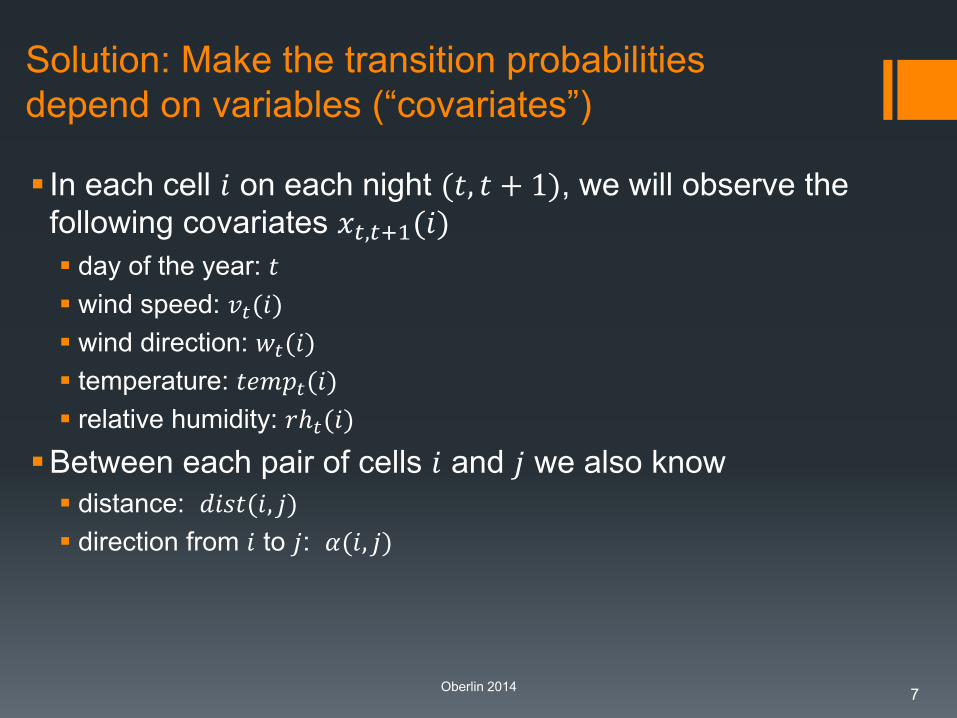
Solution: Make the transition probabilities

depend on variables (“covariates”)

In each cell 𝑖 on each night (𝑡, 𝑡 + 1), we will observe the

following covariates 𝑥𝑡,𝑡+1(𝑖)

day of the year: 𝑡

wind speed: 𝑣𝑡(𝑖)

wind direction: 𝑤𝑡(𝑖)

temperature: 𝑡𝑒𝑚𝑝𝑡(𝑖)

relative humidity: 𝑟ℎ𝑡(𝑖)

Between each pair of cells 𝑖 and 𝑗 we also know

distance: 𝑑𝑖𝑠𝑡(𝑖, 𝑗)

direction from 𝑖 to 𝑗: 𝛼(𝑖, 𝑗)

Oberlin 2014 7

Parametric

State Transition Model Let 𝛼(𝑖, 𝑗) be the heading from 𝑖 to 𝑗

Let 𝑤(𝑖) be the heading of the wind

Let 𝑣(𝑖) be the speed of the wind

Wind profit 𝑣(𝑖) cos 𝑤 𝑖 − 𝛼 𝑖, 𝑗

1 if perfectly aligned

−1 if perfect headwind

Oberlin 2014 8

𝑖

𝑗

𝛼

-3 -2 -1 0 1 2 3

-1.0

-0.5

0.0

0.5

1.0

x

cos(

x)

𝑤 𝑗 − 𝛼(𝑖, 𝑗)

cos𝑤𝑗−𝛼𝑖,𝑗

𝑤

Distance Preferences

Desirability(𝑑𝑖𝑠𝑡) = 𝑁𝑜𝑟𝑚𝑎𝑙 log 𝑑𝑖𝑠𝑡 ; 𝜇, 𝜎

Oberlin 2014 9

0 100 200 300 400

0.00

00.

002

0.00

40.

006

0.00

80.

010

Index

dlno

rm(1

:400

, 5, 0

.25)

Distance

Desir

abili

ty

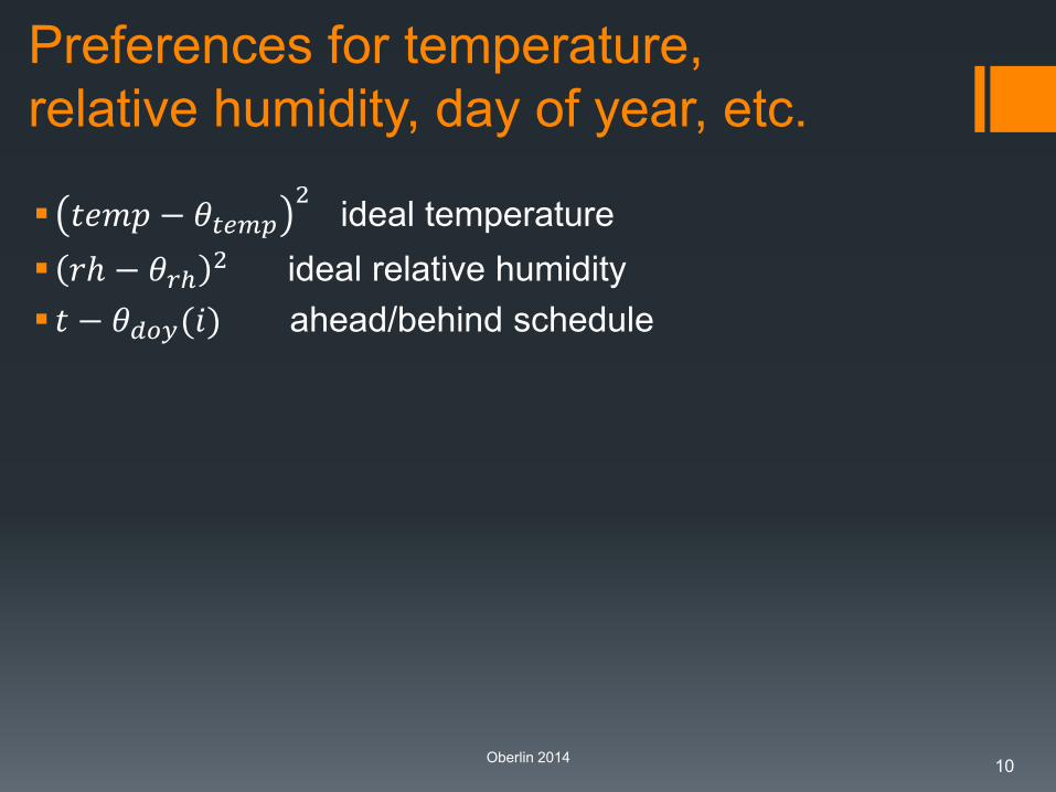
Preferences for temperature,

relative humidity, day of year, etc.

𝑡𝑒𝑚𝑝 − 𝜃𝑡𝑒𝑚𝑝2 ideal temperature

𝑟ℎ − 𝜃𝑟ℎ2 ideal relative humidity

𝑡 − 𝜃𝑑𝑜𝑦(𝑖) ahead/behind schedule

Oberlin 2014 10

Combine into probability model

𝐹 𝑖, 𝑗 = 𝛽0 + 𝛽𝑤𝑣𝑡(𝑖) cos 𝑤𝑡 𝑖 − 𝛼 𝑖, 𝑗 +𝛽𝑑Normal log 𝑑𝑖𝑠𝑡 𝑖, 𝑗 ; 𝜇𝑑𝑖𝑠𝑡, 𝜎𝑑𝑖𝑠𝑡 +

𝛽𝑡𝑒𝑚𝑝 𝑡𝑒𝑚𝑝𝑡 − 𝜃𝑡𝑒𝑚𝑝2+ 𝛽𝑟ℎ 𝑟ℎ𝑡 − 𝜃𝑟ℎ

2 +

𝛽𝑑𝑜𝑦 𝑡 − 𝜃𝑑𝑜𝑦(𝑖) +⋯

𝑃 𝑠𝑡 = 𝑗 𝑠𝑡−1 = 𝑖 =exp 𝐹 𝑖,𝑗

exp 𝐹 𝑖,𝑗′𝑗′

Construct the transition matrix at time 𝑡 by evaluating this function for each pair (𝑖, 𝑗)

Oberlin 2014 11

Step 2: Fitting the model to data

The data we wish we had:

Tracks of individual birds

over time

Weather at every location

12 Oberlin 2014

macworld.com

www.azoresbioportal.angra.uac.pt

This would give us points

(𝑥𝑡,𝑡+1 𝑖 , 𝑠𝑡 𝑖 , 𝑠𝑡+1 𝑗 ) to

which we could fit our model

The data we have (1):

Project eBird (www.ebird.org)

Volunteer Bird Watchers

Stationary Count

Travelling Count

Time, place, duration, distance

travelled

Species seen

Number of birds for each

species or ‘X’ which means ≥ 1

Checkbox: This is everything

that I saw

8,000-12,000 checklists

uploaded per day

13 Oberlin 2014

The data we have (2):

Weather Radar

Radar detects

weather (remove)

smoke, dust, and insects (remove)

birds and bats

Removing weather

manual, using a web-based tool

Removing smoke, dust & insects

estimate velocities

ignore pixels that are moving at same speed as wind

Oberlin 2014 14

The data we (hope to) have (3):

Acoustic monitoring

Night flight calls

People can identify species or

species groups from these calls

Oberlin 2014 15

The data we have (4):

Weather data

North American Regional Reanalysis

wind speed

wind direction

temperature

relative humidity

Oberlin 2014 16

Modeling for each data source (1):

eBird

Bird watchers do not detect all birds at a given location

detection probability

day of year

weather conditions

habitat (shoreline, meadow, dense forest)

expertise of the bird watcher

Bird watchers may misidentify species

Yu, J., Wong, W-K., and Hutchinson, R. (2010). Modeling Experts and Novices in Citizen Science Data for Species

Distribution Modeling. Proceedings of the 2010 IEEE International Conference on Data Mining

Yu, J., Wong, W-K. and Kelling, S. (2014). Clustering Species Accumulation Curves to Identify Skill Levels of Citizen

Scientists Participating in the eBird Project. IAAI 2014

Yu, J., Hutchinson, R. and Wong, W-K. (2014). A Latent Variable Model for Discovering Bird Species Commonly

Misidentified by Citizen Scientists. AAAI 2014

Oberlin 2014 17

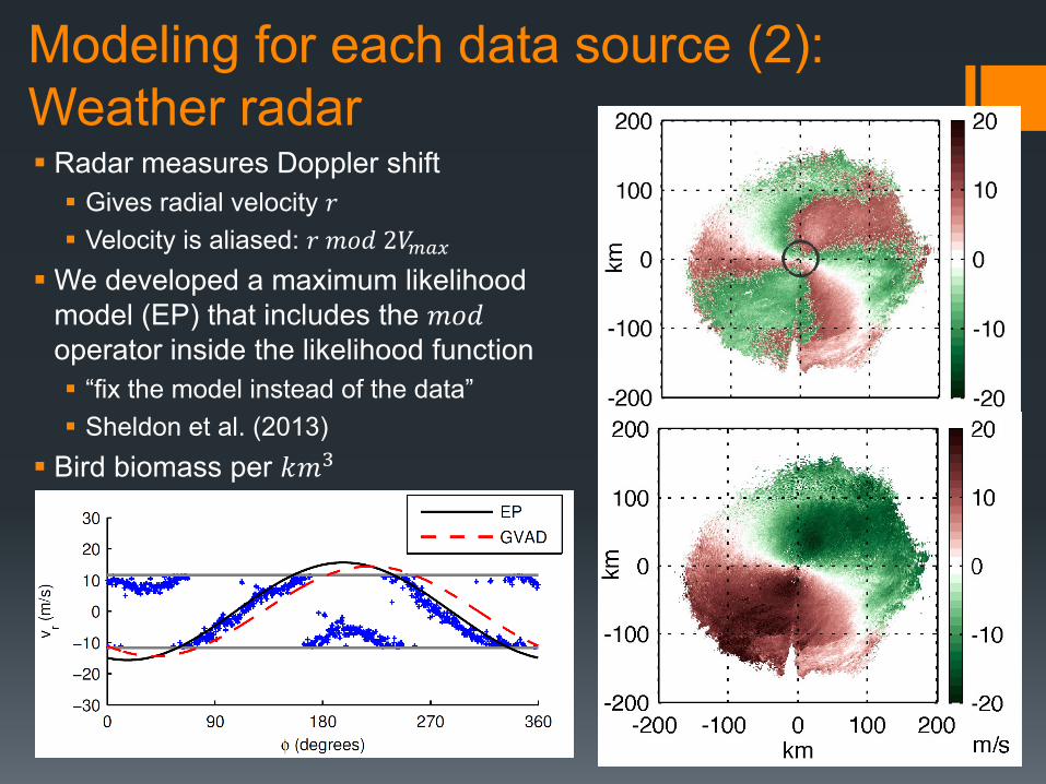
Modeling for each data source (2):

Weather radar Radar measures Doppler shift

Gives radial velocity 𝑟

Velocity is aliased: 𝑟 𝑚𝑜𝑑 2𝑉𝑚𝑎𝑥

We developed a maximum likelihood

model (EP) that includes the 𝑚𝑜𝑑 operator inside the likelihood function

“fix the model instead of the data”

Sheldon et al. (2013)

Bird biomass per 𝑘𝑚3

Oberlin 2014 18

Radar Visualization

Oberlin 2014 19

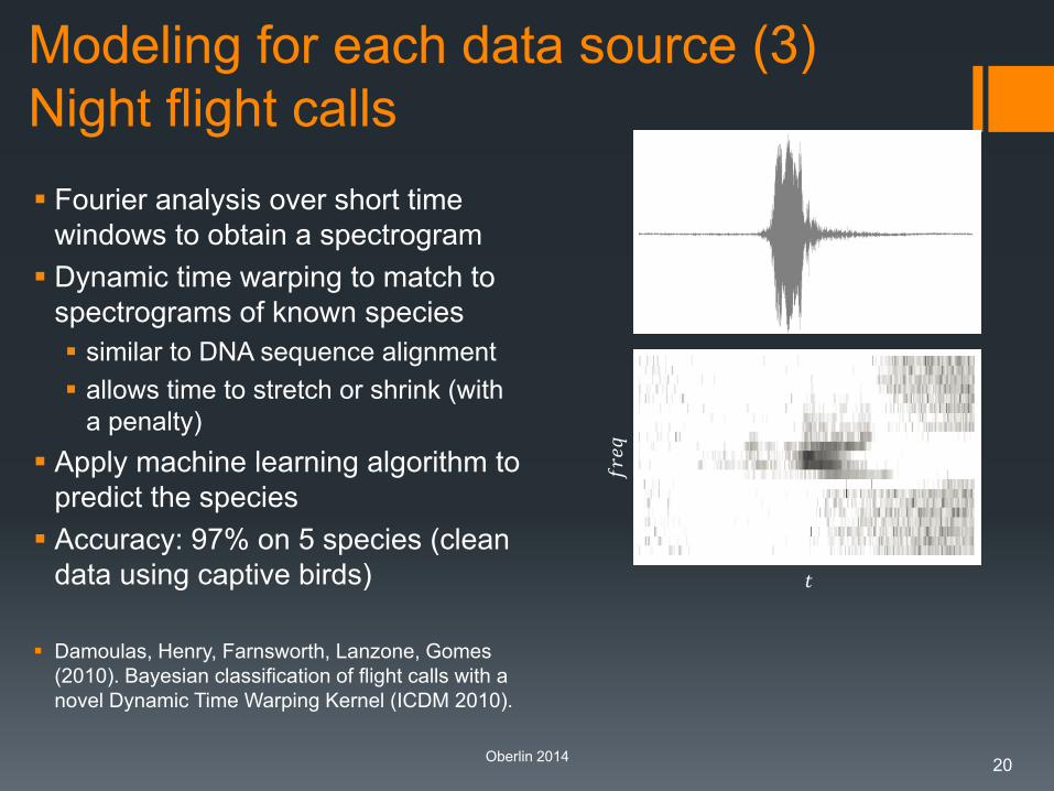
Modeling for each data source (3)

Night flight calls

Fourier analysis over short time

windows to obtain a spectrogram

Dynamic time warping to match to

spectrograms of known species

similar to DNA sequence alignment

allows time to stretch or shrink (with

a penalty)

Apply machine learning algorithm to

predict the species

Accuracy: 97% on 5 species (clean

data using captive birds)

Damoulas, Henry, Farnsworth, Lanzone, Gomes

(2010). Bayesian classification of flight calls with a

novel Dynamic Time Warping Kernel (ICDM 2010).

Oberlin 2014 20

𝑡

𝑓𝑟𝑒𝑞

Modeling for each data source (4)

NARR data

NARR data product is the result of

performing “data assimilation”

Observed variables from radiosonde

balloons

Update a physics-based model of the

atmosphere via Bayes theorem

Oberlin 2014 21

www.ncdc.noaa.gov

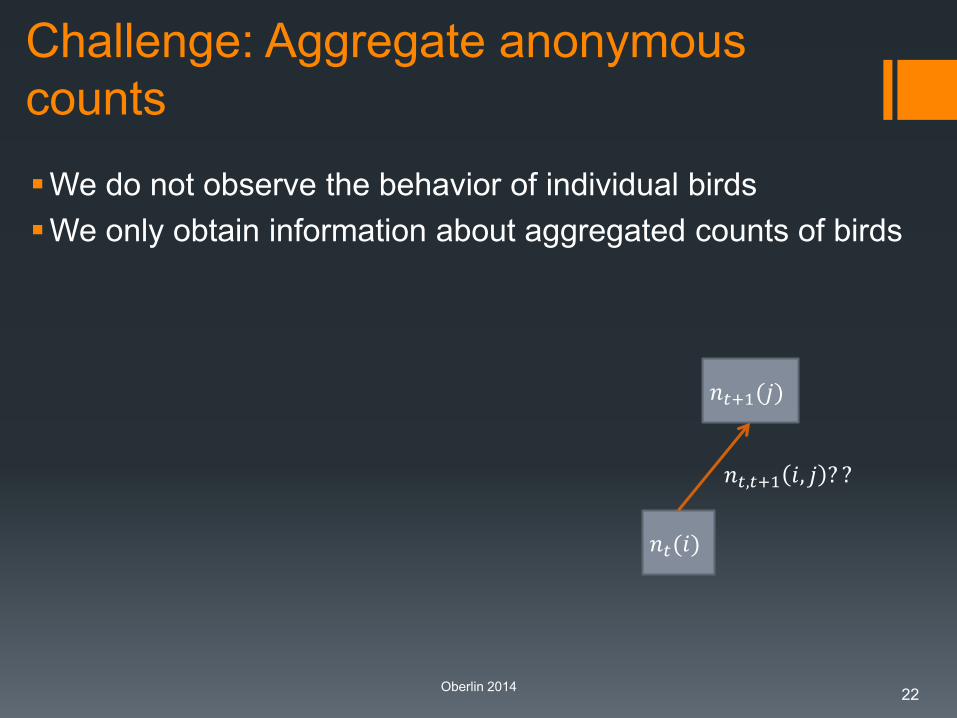
Challenge: Aggregate anonymous

counts

We do not observe the behavior of individual birds

We only obtain information about aggregated counts of birds

Oberlin 2014 22

𝑛𝑡(𝑖)

𝑛𝑡+1(𝑗)

𝑛𝑡,𝑡+1 𝑖, 𝑗 ? ?

Solution:

Collective Graphical Models

New method for fitting models of individual behavior

from noisy aggregate counts

Assumes all birds make their decisions independently

according to the same 𝑃 𝑠𝑡+1 = 𝑗 𝑠𝑡 = 𝑖, 𝑥𝑡,𝑡+1(𝑖, 𝑗)

Oberlin 2014 23

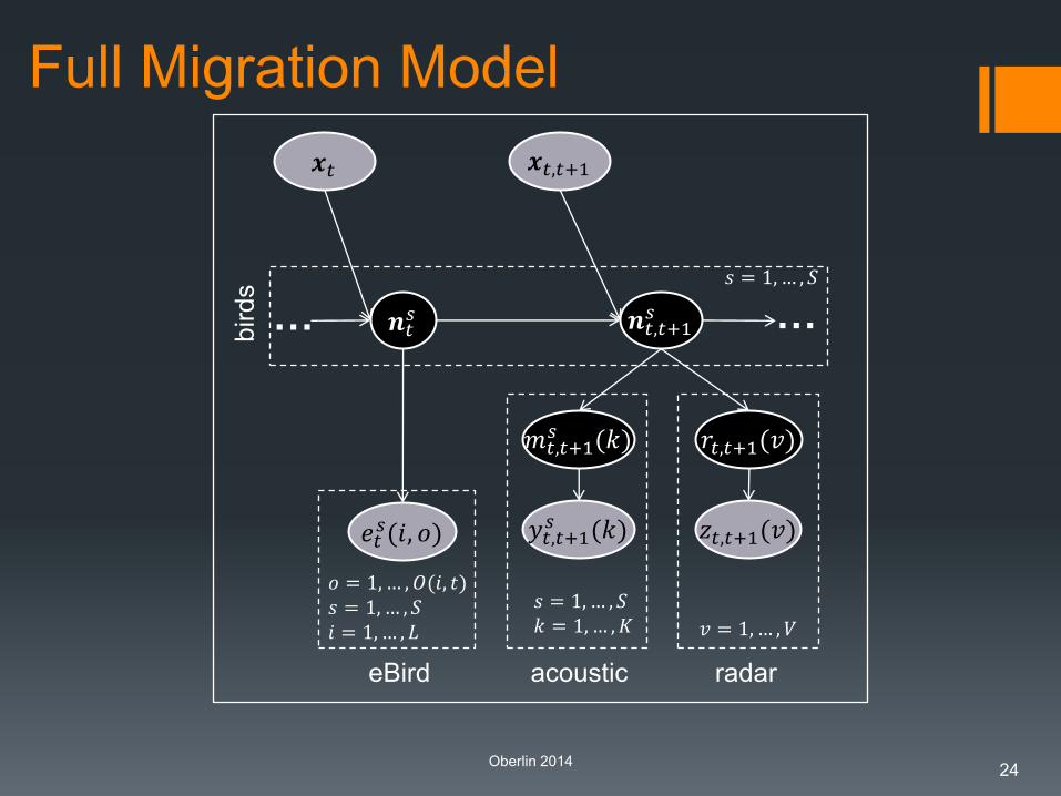
Full Migration Model

Oberlin 2014 24

𝒏𝑡𝑠 𝒏𝑡,𝑡+1

𝑠

𝑒𝑡𝑠(𝑖, 𝑜)

𝑠 = 1,… , 𝑆

𝑚𝑡,𝑡+1𝑠 (𝑘)

𝑦𝑡,𝑡+1𝑠 (𝑘)

𝑟𝑡,𝑡+1 (𝑣)

𝑧𝑡,𝑡+1 (𝑣)

… …

𝑜 = 1,… , 𝑂(𝑖, 𝑡) 𝑠 = 1,… , 𝑆 𝑖 = 1, … , 𝐿

𝑠 = 1,… , 𝑆 𝑘 = 1,… , 𝐾 𝑣 = 1,… , 𝑉

eBird acoustic radar

bird

s

𝒙𝑡,𝑡+1 𝒙𝑡

Fitting Latent Variable Models

Expectation Maximization (EM; MAP version)

1. Make initial guess about the parameter values

Θ = 𝛽0, 𝛽𝑤 , 𝛽𝑡𝑒𝑚𝑝, 𝜃𝑡𝑒𝑚𝑝, 𝛽𝑟ℎ , 𝜃𝑟ℎ , 𝛽𝑑𝑜𝑦 , 𝜃𝑑𝑜𝑦(𝑖), 𝛽𝑑𝑖𝑠𝑡 , 𝜇𝑑𝑖𝑠𝑡 , 𝜎𝑑𝑖𝑠𝑡

2. Compute the most likely number of birds flying from cell 𝑖 to

cell 𝑗 each night (for all 𝑖, 𝑗). 𝒏𝑡,𝑡+1𝑠 (𝑖 → 𝑗).

“Maximum Aposteriori Probability (MAP) estimate”

3. Pretend these are the true values of the latent variables

and adjust the parameters Θ to maximize the likelihood of

the 𝒏𝑡,𝑡+1𝑠 𝑖 → 𝑗 values:

argmaxΘ𝑃 𝒏𝑡,𝑡+1𝑠 Θ

4. Repeat 2-3 until convergence

Oberlin 2014

25

“E-Step”

Very Difficult

“M-step”

Easy: Can be

solved with

gradient

descent

Intractability of the E step in the

Collective Graphical Model

Let 𝑀 be the population size

Let 𝐿 the number of grid cells

Theorem: Unless 𝑃 = 𝑁𝑃, there is no exact

inference algorithm with runtime that is

simultaneously polynomial in both 𝑀 and 𝐿

Bird migration has 𝑀 ≈ 109 and 𝐿 = 1008

We must approximate!!

Oberlin 2014 26

Approximation #1:

Markov Chain Monte Carlo (MCMC)

Algorithm (Sheldon & Dietterich, NIPS 2011)

Samples from 𝑃(𝒏𝑡,𝑡+1|𝒏1, … , 𝒏𝑇)

posterior distribution of “flows” from

cell to cell

respects Kirchoff’s laws

running time is independent of

population size

converges (slowly) to the correct

distribution

Oberlin 2014 27

101

102

100

102

104

Population size

Se

co

nd

s

VE

MCMC

Best exact method

Our method

(to 2% relative error)

Approximation #2:

MAP approximation (Sheldon, Sun, Kumar, Dietterich, ICML 2013)

Approximate MAP inference Continuous relaxation (allow counts to

be real numbers)

Sterling’s approximation: log 𝑛! ≈𝑛 log 𝑛 − 𝑛

Theorem: With these two

approximations, the CGM log

likelihood is convex

Solve using Matlab interior point

solver

Oberlin 2014 28

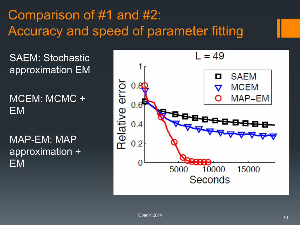
Comparison of #1 and #2:

Accuracy and speed of parameter fitting

SAEM: Stochastic

approximation EM

MCEM: MCMC +

EM

MAP-EM: MAP

approximation +

EM

Oberlin 2014 30

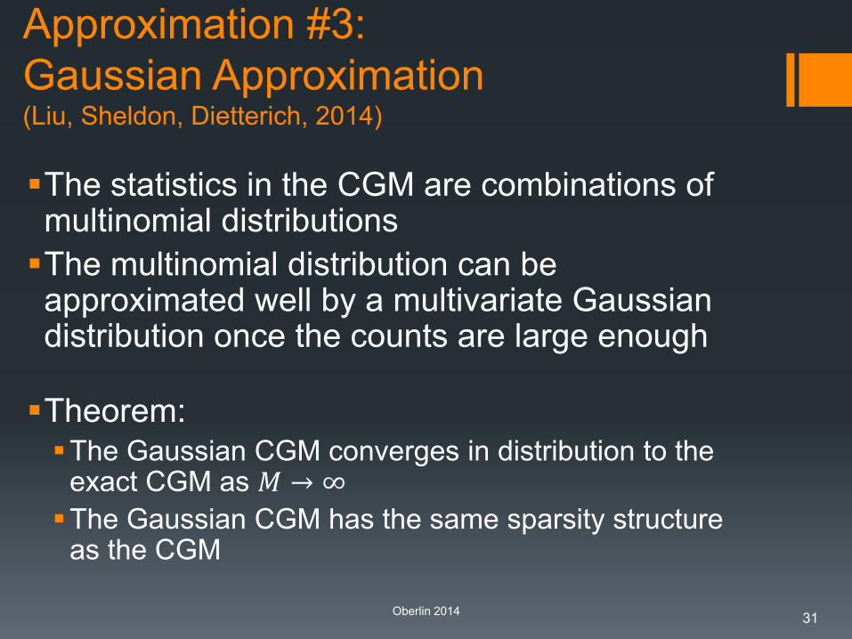
Approximation #3:

Gaussian Approximation (Liu, Sheldon, Dietterich, 2014)

The statistics in the CGM are combinations of multinomial distributions

The multinomial distribution can be approximated well by a multivariate Gaussian distribution once the counts are large enough

Theorem: The Gaussian CGM converges in distribution to the

exact CGM as 𝑀 → ∞

The Gaussian CGM has the same sparsity structure as the CGM

Oberlin 2014 31

Comparison of #2 and #3:

Fitting the parameters

If 𝑀 is too small,

both the MAP

approximation and

the GCGM lose

badly, but GCGM is

much worse

For 𝑀 ≥ 480, GCGM gives

answers identical to

those of the MAP

approximation

Oberlin 2014 32

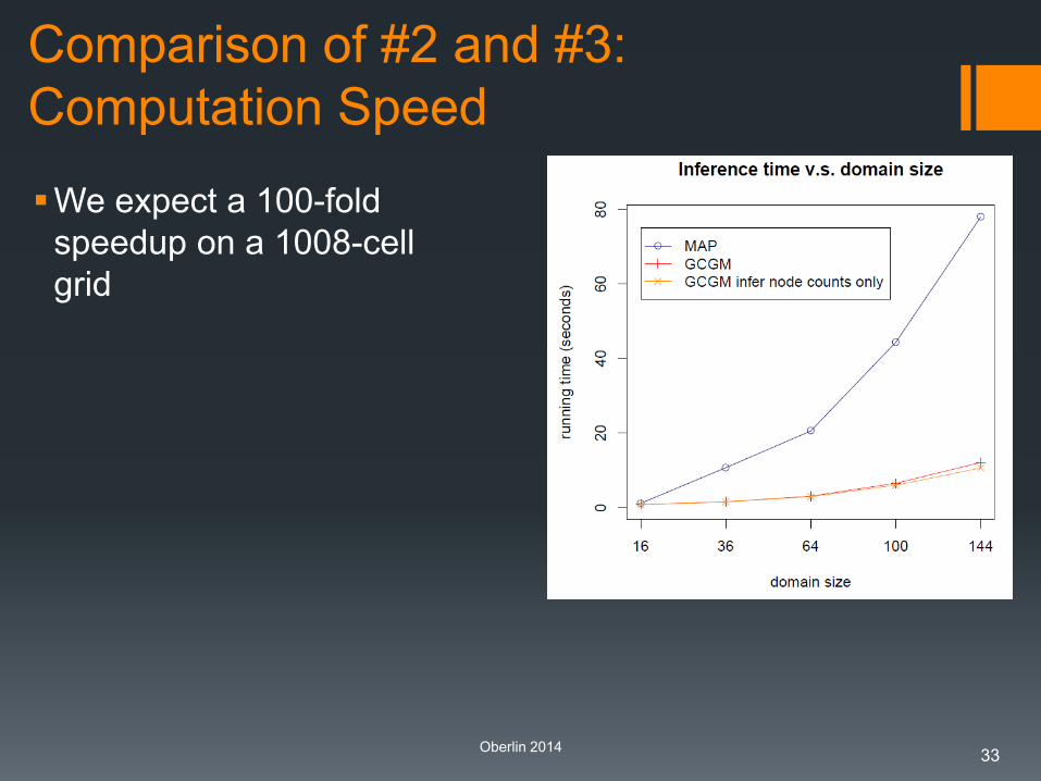
Comparison of #2 and #3:

Computation Speed

We expect a 100-fold

speedup on a 1008-cell

grid

Oberlin 2014 33

Black-throated Blue Warbler

Initial Results:

Movement Reconstruction [Sheldon, 2009]

Observations (eBird volunteers) Fitted Migration Model

34 Oberlin 2014

Current Status

We have developed a faster algorithm for the MAP

approximation (approximation #4)

We are currently fitting both the MAP (#2) and GCGM (#3)

methods to the eBird data

Oberlin 2014 35

Step 3: Policy Optimization

Policy Questions:

1. Where should conservation reserves and habitat

restoration be performed?

Examine which cells are being used by the birds

We have also developed habitat models directly from eBird data

2. Where should wind farms be located?

3. When and where should low-altitude flight training be

allowed?

4. When should wind turbines be operated?

5. When should lights in skyscrapers be turned off?

6. Where should I go bird watching if I want to see species 𝑠?

Oberlin 2014 36

Summary

Modeling:

Non-linear probabilistic model of the behavior of individual birds

Collective graphical model (in order to work with aggregate data)

Fitting to Data:

EM algorithm

Computational complexity requires developing algorithms for

approximate inference

Policy Optimization:

Straightforward in this application Oberlin 2014

37

Mathematical

Modeling

Model Fitting

to Data

Policy

Optimization

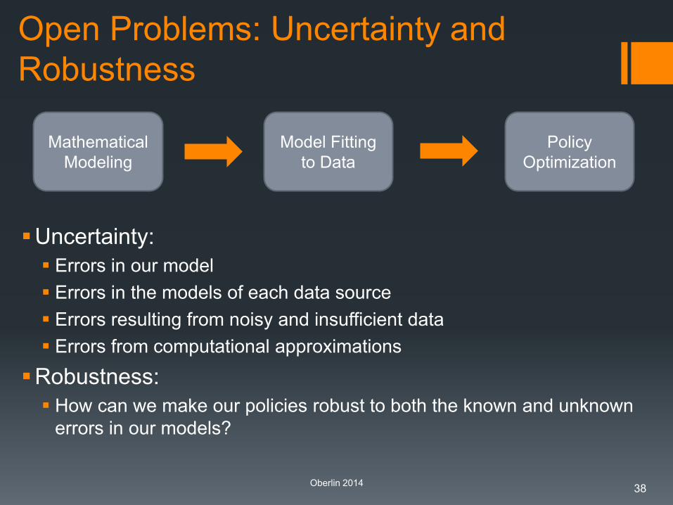
Open Problems: Uncertainty and

Robustness

Uncertainty:

Errors in our model

Errors in the models of each data source

Errors resulting from noisy and insufficient data

Errors from computational approximations

Robustness:

How can we make our policies robust to both the known and unknown

errors in our models?

Oberlin 2014 38

Mathematical

Modeling

Model Fitting

to Data

Policy

Optimization

Opportunities at Oregon State

“Spring Break Class in Monte Carlo AI”

http://web.engr.oregonstate.edu/mcai

Summer REU program: Eco-

Informatics Summer Institute

http://eco-

informatics.engr.oregonstate.edu/

PhD and Postdoc Research Projects

Fundamental research in machine

learning and AI with applications in

sustainability

Oberlin 2014

39

Thank-you

Dan Sheldon, Akshat Kumar, Liping Liu, Tao Sun: Collective Graphical

Models

Steve Kelling, Andrew Farnsworth, Wes Hochachka, Daniel Fink:

BirdCast

Carla Gomes for spearheading the Institute for Computational

Sustainability

National Science Foundation Grants 0705765, 0832804, 0905885,

1331932

40 Oberlin 2014

Questions?

Oberlin 2014 41

Mathematical

Modeling

Model Fitting

to Data

Policy

Optimization