modeling and understanding the time evolution of real ... · modeling and understanding the time...

WHITE PAPER

Mathematical Simulation ModelsModeling and Understanding the Time Evolution of Real-World Systems

Table of Contents Introduction .................................................................................................................. 1 Structural Properties Contributing to Complexity in Dynamical Systems .................... 2

System Delays ........................................................................................................ 2 Feedback Structure ................................................................................................. 2 Nonlinearity ............................................................................................................. 3 The Need for Mathematical Simulation Models ....................................................... 5

A Dynamical System .................................................................................................... 7

Simulation Models Using SAS® ................................................................................... 9

A Simulation Model Using Ordinary Differential Equations: Production, Inventory and Workforce Alignment ...................................................................................... 10

Scenario I .......................................................................................................... 13 Scenario II ......................................................................................................... 16

A Discrete Event Simulation Model ....................................................................... 20 Conclusion ................................................................................................................. 24 References ................................................................................................................ 25 Appendix A ................................................................................................................ 26

Model .................................................................................................................... 26 Constants .......................................................................................................... 26 Auxiliaries.......................................................................................................... 26 Differential Equations ........................................................................................ 26 Initial Values ...................................................................................................... 26

Appendix B ................................................................................................................ 27 Appendix C ................................................................................................................ 28

This paper was written by Christian Haxholdt, Principal Analytical Consultant in Professional Services & Delivery, Global Forecasting Solutions Practice, at SAS

Mathematical Simulation Models

1

Introduction This white paper presents simulation in an illustrated format for those needing to model and understand the time evolution of real-world systems. We define a system as a structure with a set of components – e.g., people, machines or other entities – that act and react together to produce results not obtainable by the components alone toward the achievement of some rational end.1

When we are confronted with the dynamics of reality, we quickly find ourselves surrounded by problems that fall outside the domain of traditional closed-form analysis and that are better tackled by numerical simulation of mathematical models. Using a mathematical model can help us understand the representation of a system in terms of logical and quantitative relationships that can be transformed so we can see how responses change with the use of different assumptions. From the model, we will learn about the reaction of the real system. This inference is, of course, done with the conjecture that the mathematical model is a valid representation of the real system under scrutiny.

We live in a fairly complex, dynamic reality of natural and social systems. Most systems are not in equilibrium, and their states change continuously. There have always been changes in society and the economy, but over the last few decades, these changes have seemed to happen much more rapidly. The rate of change reflects itself in the speed at which organizations grow, develop, organize and plan. We might even claim that the greatest constant in today’s environment is change.2 The rapid rate of change provides ever-increasing management challenges. One of the key differences between managers who are successful and those who are not is their ability to address changes before it is too late. However, it is very hard – and sometimes impossible – for decision makers to process the variety and complexity of the systems experiencing problems.

When we refer to complexity, we mean dynamic complexity due to the interaction between system components. We do not mean combinatorial or detail complexity, such as scheduling an airline’s crews and flights, where the complexity lies in finding the best among many feasible solutions. We know from physics that dynamic complexity, compared to combinatorial complexity, arises even in simple systems with only a few interacting components, e.g., a forced damped pendulum.

Another example can be found in The Beer Distribution Game,3 a role-playing simulation of an industrial production and distribution system developed at MIT. The system rules of this very simple game can be explained in just a few minutes; yet, the game enables us to observe the complex and dysfunctional behaviors that arise from player interactions over time.

1 (Schmidt, 1970) 2 (Sterman, 2000) 3 (Sterman, 1989)

SAS White Paper

2

Structural Properties Contributing to Complexity in Dynamical Systems There are three main kinds of structural properties that contribute to complexity in dynamical systems: system delays, feedback structure and nonlinearity.

System Delays

A delay is a process whose output – a piece of information or material – lags behind its input. A delay indicates that something is accumulating between the inflow and outflow. Delays give systems inertia. Delays are pervasive.4

• It takes time to measure and report information.

• It takes time to make decisions.

• It takes time for decisions to affect the state of a system.

Suppose there is a sudden and unexpected increase in the demand for a manufacturing company’s products. There is a delay in realizing the change in demand, another delay to get the necessary investments to increase production capacity and, finally, there is a delay in building new capacity.

Delayed reactions typically create instability – i.e., cause systems to over- and undershoot desired levels – exhibiting oscillatory behavior and even bringing danger if not properly understood.

Feedback Structure

To determine a system’s dynamics, we must understand the feedback structure. Feedback is the interaction among system components. Real-world systems are usually characterized by circular causality. Intuitively, a feedback loop exists when the dynamical behavior of one component is transmitted to the next until a signal is returned in a modified form to its origin, thus closing the loop and potentially influencing a new undertaking. One might expect a range of different feedback structures, but in reality there are only two kinds: self-reinforcing and self-correcting. If the structure’s tendency is to reinforce the initial action, the feedback is self-reinforcing. If the tendency is to oppose it, the feedback is self-correcting.

Self-reinforcing loops amplify system behavior. For example, a software company’s growth strategy includes R&D investments. The assumption is that as R&D investments are made, new product introductions will increase. As new product introductions increase, sales will also increase. As sales increase, revenues increase. Because a percentage of those revenues are allocated for R&D, investments in R&D increase – and we have a full loop. By itself, ignoring limits to growth, the system will grow exponentially.

4 (Sterman, 2000)


3

The self-correcting loop counteracts change. In a typical manufacturing company, the management of inventory levels demonstrates a self-correcting process. When actual inventory exceeds the desired level, the gap between desired and actual inventory levels will increase. Inventory levels are then adjusted by holding back production. The adjustments will again align the level of actual inventory with the desired level – and we have a full loop.

A self-correcting loop can be identified by its goal-seeking behavior. If certain conditions keep coming back to some kind of “norm” no matter what anyone does, then a self-correcting process is probably at work. Similarly, if conditions seem to resist change, if growth falters or never quite takes off, or if unproductive behavior is never stopped, then a strong self-correcting dynamic is likely present.

As a last example, let’s combine the two feedback structures. To generate more sales, a company hired an advertising agency. Initial efforts succeeded in generating more sales. However, additional sales meant more resources needed to go into advertising. Eventually, the advertising campaign saturated the market and reached its total market size. The company then faced the more difficult task of taking customers away from competitors and soon realized that even if it were to capture all of the customers, it would still be limited by total market size. The company experiences a period of accelerating expansion. The expansion slows and eventually halts, possibly even reversing itself in an accelerating collapse – i.e., a reverse self-reinforcing loop. The growth phase is caused by one or more reinforcing feedback processes. The slowdown is due to a self-correcting process brought on as a limit is approached. The limit may be a resource constraint or an external or internal response to growth. The accelerating collapse, if and when it occurs, arises from the reinforcing process operating in reverse, generating more and more contraction.

As mentioned, self-correcting feedback can be characterized as a goal-seeking, equilibrating or stabilizing process, and it can sometimes generate oscillations. Reinforcing loops are sources of growth or accelerating collapse – i.e., they are destabilizing. Combined, reinforcing and self-correcting feedback processes can generate an extreme variety of different dynamical patterns. Therefore, when we try to manage a feedback system, our actions are typically amplified or counteracted, depending on which feedback structures are dominating the system at the time.

Nonlinearity

Nonlinearity implies that system variables or attributes affect each other in non-proportional ways, and that they interact so that their partial effects cannot be easily differentiated over time. Nonlinear interactions may cause changes in the structural dominance of a system. Substructures that have dominated a system's behavior in one instance suddenly or gradually lose influence while other substructures gain influence, causing a dramatic modification of the system's dynamic response.

Together, these complex system characteristics – delays, feedback and nonlinearities – tend to disguise the relationship between cause and effect, thus obscuring current problems. A successful solution can often seem counterintuitive and may be hard to identify. In addition, there are always uncertainties associated with real-world systems, and humans have a tendency to state their perceptions, policies,

SAS White Paper

4

preferences and attitudes vaguely. Consequently, what we might call realistic system models require the use of random variables in simulation models.

Note that we only mentioned randomness at the end of this discussion and not explicitly as a cause of dynamic complexity. This is intentional; while this position may be controversial to some, we really don’t need any randomness to make a dynamical system complicated.

To illustrate, consider this logistic mapping:

𝑥𝑛+1 = 𝛼 × 4 × (1 − 𝑥𝑛) 𝛼 ∈ [0,1]

The equation is a difference equation or an iterated map function. It maps one value of 𝑥 (𝑥0 ) in the range 0 ≤ 𝑥 ≤ 1 by iterating the mathematical operations into another value (𝑥1) in the same range. We will not provide a detailed discussion of the logistic function. We only show what happens to the long-run behavior of the function as we gradually increase the parameter 𝛼 up toward 1.

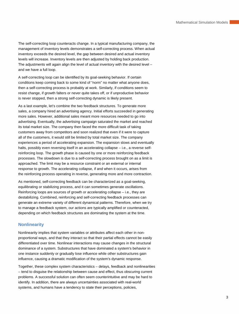
In Figure 1, we see that the eventual behavior of the function is just a single value up to and around 𝛼 ≈ 0.75, where afterward the system experiences a double period – also called a bifurcation (the oscillation back and forth between two values). Finally, after infinitely many bifurcations, the value never seems to repeat itself and is practically indistinguishable from pure randomness – the behavior is chaotic. As 𝛼 gets closer to 1, the solution of 𝑥 will keep oscillating between bands of periodic and chaotic behavior.

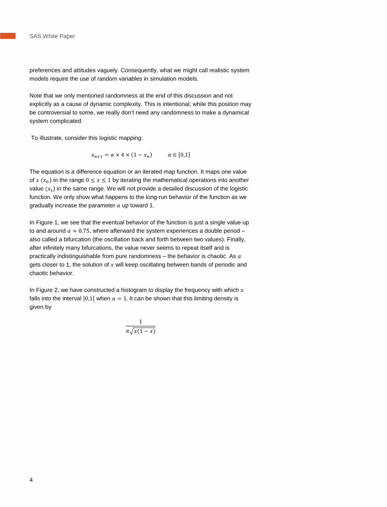
In Figure 2, we have constructed a histogram to display the frequency with which 𝑥 falls into the interval ]0,1[ when 𝛼 = 1. It can be shown that this limiting density is given by

1𝜋�𝑥(1 − 𝑥)


5

Figure 1: Diagram showing the behavior of 𝒙 for different values of 𝜶.

Figure 2: Histogram of 𝒙 when 𝜶 = 𝟏

The Need for Mathematical Simulation Models If a problem is simple enough, it might be analytically tractable, like the logistics map function. This means that we can use mathematical methods – such as algebra, calculus or probability – to find an analytical solution. However, in order to understand, adapt to and control these highly complex, real-world systems – where predictions of the effects of decisions on performance are practically impossible, and where any decision can have a profound impact on profitability, market share, operation, supply chain, customer satisfaction and other key factors in an organization’s success – we must take advantage of mathematical simulation models.

SAS White Paper

6

Although the simulation model is a simplified version of reality, it can still be realistic, making it a formidable tool for testing and evaluating different system configurations, implications of operational or policy changes, and their effects on future results.

Mathematical simulation models are unlimited creative instruments that can explicitly represent, capture, combine and formalize any structure we might consider. Also, models, in contrast to an abstract flow chart, make it easier to communicate assumptions to decision makers who may again subject the assumptions to constructive criticism and change.

Training with a simulation model enables a better understanding of dynamical behavior in a system, and can also help foster a shared understanding across functional teams in an organization. Mathematical simulations can complement traditional work methodologies by providing managers with the hands-on experience of testing their decisions in a simulated organization. Other than providing a low-cost company flight simulator,5 a simulation:

• Allows time and space to be compressed or dilated.

• Enables the repetition of actions under same or different conditions with the ability to stop actions to reflect on results.

• Lets you experiment with decisions that are dangerous, infeasible or unethical in the real system or try strategies that we presume will lead to poor performance.

• Enables you to push the system into extreme conditions, i.e., experience catastrophes in advance, which often reveals more about structure and dynamics than incremental adjustments to successful strategies.

Today’s world is more interconnected – we can’t just do one thing. Industries increasingly overlap and merge, product life cycles shorten, development costs increase, new organizational structures appear and the influence of different stakeholder groups transforms and changes quickly. This rapidly changing environment has created a need for a different – but complementary – way of approaching complex systems to increase the efficiency of decision making.

Mathematical simulation seems to offer significant flexibility in the modeling of complex operational conditions and, in particular, is able to handle various forms of the unavoidable uncertainty. We need to see and understand the big picture.

5 (Sterman, 1989)


7

In the remainder of this paper, we will introduce a dynamical system that will serve as the foundation for the mathematical models we develop. We will also illustrate the use of simulation with two different examples using SAS®:

1. A continuous model that uses ordinary differential equations and contains all the ingredients that make dynamical systems complicated – delay, feedback and nonlinearity.

2. A discrete event model, which in our example does not contain any feedback, but still lends itself to relevant use in scenario analysis.

A Dynamical System We will begin with a somewhat formal definition of a dynamical system. First, a dynamical system is one whose states change with time – in contrast to a static system in which time plays no role. To define a general dynamical system, although we restrict our attention to finite dimensional systems, we must introduce three concepts:6

• State space. The elements of a state space represent possible states of the system. In probability theory, this is known as the sample space – i.e., the set of all possible outcomes of an experiment.

• Time. For the concept of time, we will take a practical approach and focus on time that extends into the future only and not the past – i.e., the system might potentially be irreversible.

• Time-evolution operator. The final ingredient – a time-evolution operator or law of motion – is a set of rules that allows us to determine the state of the system for each moment of time, from its state at a previous time. We assume that the result of an operator will depend only on the initial condition of the system and the length of the evolution, not on the moment when the state of the system was initially registered.

A finite dimensional dynamical system’s states change in accordance with a set of appropriate operators, and it can be completely characterized by a set of observables or state variables, 𝑥1, 𝑥2, … , 𝑥𝑛. One evolutionary history of the system is given by a time series 𝑥1(𝑡), 𝑥2(𝑡), … , 𝑥𝑛(𝑡) that forms a trajectory in an n-dimensional state space, with t indicating the time.

An operator is deterministic if it does not contain a random component. The time evolution of a deterministic dynamical system is always completely determined by its current state and past history; therefore the entire history (past, present and future) of the system is represented by a certain trajectory in state space, once an initial state is given. However, in practice we never really have the luxury of enough information for such complete determination. Strictly speaking, a deterministic model can only be justified if it is able to produce an outcome close to, or equal to, some “true” mean outcome. However, that might actually be meaningless, because normally when we refer to a mean outcome, we refer to a probabilistic expectation – a term not even defined in relation to a deterministic model.

6 (Katok & Hasselblatt, 1996)

SAS White Paper

8

With a stochastic model, it will be meaningful (and, in principle, possible) to determine a mean outcome. This is “true” at least within the framework specified by the stochastic model, which implies that we usually are forced to abandon the deterministic study of one point in state space in favor of a probabilistic study of a subset of state space. Therefore, any solution of a stochastic model must involve some randomness, and we can only hope to determine something about the probability distributions of the solution. The key here is, instead of asking, “What will the state of the system be at time t?” is to ask the more appropriate question: “What is the probability that at time t the state of the system will belong to a specified subset of the state space?”7

Two main types of dynamical systems are encountered in most applications: continuous and discrete. For our purpose, we think about a continuous system when the state variables change continuously over time. In a discrete system, the state variables change instantaneously at separate points in time. Few systems completely belong to one category or the other. So the decision whether to use a continuous or discrete model depends on the objective of the modeling. The examples we provide in the next section of this paper can both be modeled using continuous and discrete simulation.

When the state is continuous or can be well-approximated by a continuous state, the dynamics are usually described by an ordinary differential equation, for example:

𝑑𝐱𝑑𝑡

= 𝐟(𝐱(𝑡),𝛃(𝑡),𝐱(0), 𝑡)

• 𝐟 is the time-evolution operator.

• 𝐱(𝑡) represents the state vector of the system and takes values in the state space. • 𝛃(𝑡) is a vector of decision parameters or controls.

• 𝑡 ∈ ℝ is the time.

• 𝐱(0) is the state of initial conditions.

Note that the vector of parameters is also dynamical, i.e., a function of time. The parameter vector typically reflects an optimized set that will change over time.

To model our discrete system, we use a discrete event simulation (DEVS) model. A DEVS model can be described in a simple, abstract way by a six-tuple structure8

⟨𝑋,𝑌, 𝑆,𝑇𝑒𝑥𝑡 ,𝑇𝑖𝑛𝑡,𝑇𝑜𝑢𝑡⟩

7 (Halmos, 2006) 8 (Zeigler, Praehofer, & Kim, 2000)


9

in which:

• 𝑋 is a set of input values.

• 𝑌 is a set of output values.

• 𝑆 is a set of states.

• 𝑇𝑖𝑛𝑡: 𝑆 → 𝑆 is the internal transition function.

• 𝑇𝑒𝑥𝑡:𝑋 → 𝑆 is the external transition function.

• 𝑇𝑜𝑢𝑡: 𝑆 → 𝑌 is the output transition function.

At any time, 𝑡, the system will be in some state, 𝑠 ∈ 𝑆. The transition function 𝑇𝑒𝑥𝑡 determines the pattern in which an event with value 𝑥 ∈ 𝑋 enters the system. The transition function 𝑇𝑖𝑛𝑡 dictates the system’s change of states internally. And finally, the transition function 𝑇𝑜𝑢𝑡 determines how an event taking on value 𝑦 ∈ 𝑌 will leave the system. Clearly, these three transition functions can be dependent on each other. The discrete system is aligned with our definition of a dynamical system with a set of states and a time-evolution operator consisting of three transition functions.

Simulation Models Using SAS® In this section, we will introduce simulation using examples of a manufacturing company and a hospital MRI scanning department. Before getting to the examples, however, a few disclaimers are necessary. Because the main purpose is illustration, the models are kept small, which also means that we have imposed certain simplifying assumptions. However, even though they are small, they are by no means less relevant. Both examples are generic in structure and can be extended to fit many different real-world situations.

A simulation model can be anything from a few equations to thousands and thousands of equations. The normal procedure for very large models involves splitting the systems into smaller parts, modeling the parts separately and combining everything in the end. This procedure makes model development and debugging exercises easier.

We will illustrate mathematical simulation using two different model approaches:

1. Continuous model approach. The continuous model uses ordinary differential equations. We will develop and simulate this model type using the SAS MODEL procedure (PROC MODEL) – see Appendix B for the code. Because our interest is with the business processes, we will focus on a simple inventory/production system9 that includes workforce. This model also contains the three structural properties mentioned earlier – delay, feedback and nonlinearity – that contribute to complexity in dynamical systems.

When a company faces a problem, it is often assumed that the problem was caused by some external event. However, almost everything that goes on in a business is part of one or more systems. By taking a systems and simulation approach, we get an alternative viewpoint that indicates that the internal structure of the system often plays a larger role than external events in

9 (Arthur Andersen Business Consulting, 2000)

SAS White Paper

10

generating problems. This approach enables us to study the system and develop policies that will eliminate undesired and costly behavior.

2. Discrete event model approach. The discrete event model is simulated using SAS Simulation Studio. Our example belongs to a class of models described by queuing theory, in which customers arrive randomly at a service facility. Upon arrival, they wait in queue until served. Once served, the general assumption is that they leave the system. These queue-type models predict the behavior of systems that provide service for randomly arising demand.

To obtain knowledge about the effectiveness of the queuing system, we will measure the waiting time for a typical customer in the queue. In our example, we will simulate operations in the scanning department of a hospital. The goal is to find procedures or structures that, in the long run, will maintain waiting times at an acceptable level. This comes down to a tradeoff of better service versus the expense of providing more service capability – i.e., determining the increase in investment of service for a corresponding decrease in waiting time.

We will not model any feedback process in this system, but it is easy to visualize. The service pattern (and arrival pattern) can depend on how many are waiting for service. An employee may work faster if the line is building up (self-correcting), or he/she may become frustrated and less efficient, creating an even longer queue, which then leads to more frustration, etc. (reinforcing). The system is said to be state-dependent.

Although the production, inventory and workforce model with its feedback structure does not belong to the family of queue systems, the entities (products) and resources (workforce) are discrete events that move and interact and can therefore be modeled and simulated using a DEVS model. So for reference, the DEVS graphical footprint of the model – i.e., the SAS Simulation Studio model – is provided in Appendix C.

A Simulation Model Using Ordinary Differential Equations: Production, Inventory and Workforce Alignment

A manufacturing company would like to use simulation to better understand the interactions between orders, inventory, production levels and workforce. The company often experiences oscillations in inventory and production levels. The first step to solving this problem is to build a model that would explain the relevant interactions.

The time dimension is measured in days. Production policy comprises two components: 1) increasing or decreasing inventory to match an optimal or desired inventory level; and 2) keeping inventory high enough to cover expected demand in the future. The company carries a safety stock equal to five times the inventory on-hand to cover daily demand. Production per day is set at one-tenth of the discrepancy between desired and actual inventory plus the expected daily demand.

Assumptions about future demand are based on the current order rate. The current order rate constitutes the real demand that the company faces. Its policy to formulate


11

expected demand is simple. The company wants to correct one-twentieth of the difference between real and expected demand each week. When beliefs about future demand change, this affects the desired level of inventory and the rate at which it is produced, according to the production policy described above.

All production goes straight to storage as inventory. A product cannot go from production to a customer; it must go into inventory first. Shipments are made only from this inventory. Because the company keeps a good safety stock, it believes it can ship the necessary products to fulfill every order. Therefore, it is not concerned with backlogs and related effects. The company’s managers know that workforce policies play a major role in almost any company situation – particularly those pertaining to production and inventory, because the workforce limits how much can be produced. When demand increases, production can increase only if there are workers available to handle the increase.

Workforce productivity is a key factor in determining production. The more productive the workforce, the smaller the workforce needed to increase production. The number of workforce resources depends on how much the company wants to produce and how productive its resources are. The formulation of the production rate from above is actually the desired production rate. The company wants to produce enough to cover the discrepancy between inventory and desired inventory, as well as expected demand (with a delay to allow time to correct the discrepancy). What it actually can produce, as described above, is determined by the workforce and its productivity.

When the company knows its desired workforce size, according to the desired production rate and productivity, it can then recruit workers to expand the workforce. The company must also replace workers who leave for any reason, but recruitment is a slow process that takes 45 days to complete, while attrition occurs over a 90-day time span. Time horizon of interest is set to 365 days.

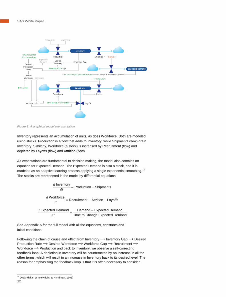
Before we attempt to determine the implications of the structure, delays and policies indicated in the business case, we must express the system in explicit quantitative form. Figure 3 illustrates the business case in a simple graphical notation that provides some structure for thinking about the dynamics. This diagram presents relationships in the actual system (the circular chains of cause and effect). The notation comprises three different elements: stocks or states (squares), flows (thick blue, straight arrows) and information (grey arrows). The other variables are auxiliary variables, decision parameters (green) and one exogenous variable – demand (red). The arrows represent the causal influences among these elements. The diagram can be used as a general way to graphically characterize any business process. It also works as a starting point for developing the quantitative model. It contains characteristics that are generally shared by all business processes and the components that make them up.

SAS White Paper

12

Figure 3: A graphical model representation.

Inventory represents an accumulation of units, as does Workforce. Both are modeled using stocks. Production is a flow that adds to Inventory, while Shipments (flow) drain Inventory. Similarly, Workforce (a stock) is increased by Recruitment (flow) and depleted by Layoffs (flow) and Attrition (flow).

As expectations are fundamental to decision making, the model also contains an equation for Expected Demand. The Expected Demand is also a stock, and it is modeled as an adaptive learning process applying a single exponential smoothing.10 The stocks are represented in the model by differential equations:

𝑑 Inventory𝑑𝑡

= Production− Shipments

𝑑 Workforce

𝑑𝑡= Recruitment− Attrition− Layoffs

𝑑 Expected Demand

𝑑𝑡 =Demand− Expected Demand

Time to Change Expected Demand

See Appendix A for the full model with all the equations, constants and initial conditions.

Following the chain of cause and effect from Inventory → Inventory Gap → Desired Production Rate → Desired Workforce → Workforce Gap → Recruitment → Workforce → Production and back to Inventory, we observe a self-correcting feedback loop. A depletion in Inventory will be counteracted by an increase in all the other terms, which will result in an increase in Inventory back to its desired level. The reason for emphasizing the feedback loop is that it is often necessary to consider

10 (Makridakis, Wheelwright, & Hyndman, 1998)


13

feedback within a business process system to understand what is causing the different patterns of behavior.

Once an explicit, mathematical description of the system has been established, the next step is to determine how the system behaves under different conditions. To do this, we will set up two different demand patterns – i.e., scenarios, one simple and one more complex – and then simulate the model.

1. Simple Scenario: The demand is initially 100 units per day on average. After 20 days, it rises to an average of 120 units per day – i.e., 20 percent – where it remains until the end of the time horizon of interest (365 days). We will run a base case and an alternate plan to improve performance of Inventory.

2. Complex Scenario: Because uncertainty is a natural substance of most real systems, we now introduce two sources of randomness in the model by making the input variables Demand and Productivity stochastic. The purpose of this scenario is to measure how uncertainty in input affects the uncertainty in outputs. Let Inventory be the output variable where we measure the uncertainty from Demand and Productivity. Assume that Demand follows normal distribution with a mean value of 100 units per day and a standard deviation equal to 20 units per day. Further assume that Productivity follows another normal distribution with a mean of six units per day and a standard deviation of 1.2 units per day.

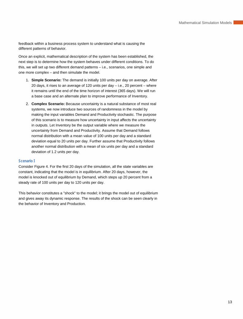
Scenario I Consider Figure 4. For the first 20 days of the simulation, all the state variables are constant, indicating that the model is in equilibrium. After 20 days, however, the model is knocked out of equilibrium by Demand, which steps up 20 percent from a steady rate of 100 units per day to 120 units per day.

This behavior constitutes a "shock" to the model; it brings the model out of equilibrium and gives away its dynamic response. The results of the shock can be seen clearly in the behavior of Inventory and Production.

SAS White Paper

14

Figure 4: Base case.

The Expected Demand shows an increase, but ever more slowly, until it approaches the new level of Demand coming in. The rate at which it increases is slowing because the flow changes Expected Demand according to the discrepancy between Demand and Expected Demand. This discrepancy is at its largest when the shock occurs. From then on, Expected Demand is growing, which makes the discrepancy smaller and smaller, thus causing less to be added to the stock each time period.

Production first rises above Demand, followed by a smaller undershoot, then continues in a slow oscillation, converging to a new equilibrium. Production is driven by Desired Inventory through Workforce. The Desired Inventory is also rising (increasing the discrepancy between Desired Inventory and actual Inventory)

100

105

110

115

120

125

130

135

0 50 100 150 200 250 300 350

Demand Expected Demand Production

100

200

300

400

500

600

700

800

0 50 100 150 200 250 300 350

Desired Inventory Inventory


15

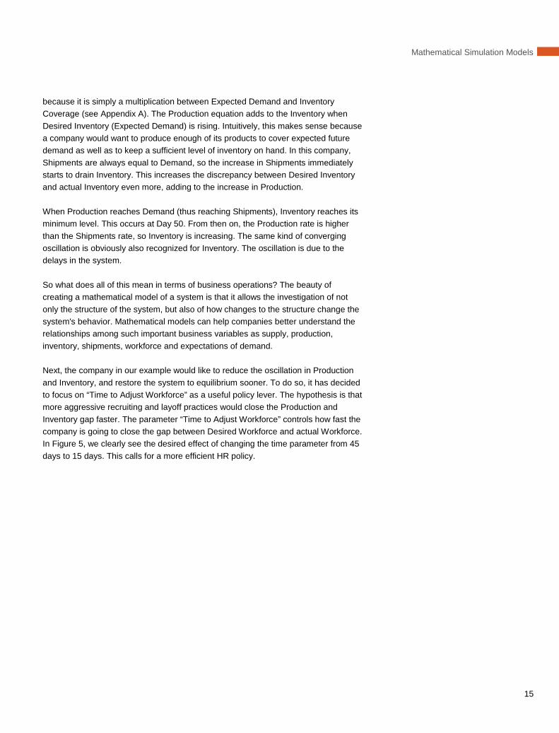
because it is simply a multiplication between Expected Demand and Inventory Coverage (see Appendix A). The Production equation adds to the Inventory when Desired Inventory (Expected Demand) is rising. Intuitively, this makes sense because a company would want to produce enough of its products to cover expected future demand as well as to keep a sufficient level of inventory on hand. In this company, Shipments are always equal to Demand, so the increase in Shipments immediately starts to drain Inventory. This increases the discrepancy between Desired Inventory and actual Inventory even more, adding to the increase in Production.

When Production reaches Demand (thus reaching Shipments), Inventory reaches its minimum level. This occurs at Day 50. From then on, the Production rate is higher than the Shipments rate, so Inventory is increasing. The same kind of converging oscillation is obviously also recognized for Inventory. The oscillation is due to the delays in the system.

So what does all of this mean in terms of business operations? The beauty of creating a mathematical model of a system is that it allows the investigation of not only the structure of the system, but also of how changes to the structure change the system's behavior. Mathematical models can help companies better understand the relationships among such important business variables as supply, production, inventory, shipments, workforce and expectations of demand.

Next, the company in our example would like to reduce the oscillation in Production and Inventory, and restore the system to equilibrium sooner. To do so, it has decided to focus on “Time to Adjust Workforce” as a useful policy lever. The hypothesis is that more aggressive recruiting and layoff practices would close the Production and Inventory gap faster. The parameter “Time to Adjust Workforce” controls how fast the company is going to close the gap between Desired Workforce and actual Workforce. In Figure 5, we clearly see the desired effect of changing the time parameter from 45 days to 15 days. This calls for a more efficient HR policy.

SAS White Paper

16

Figure 5: Scenario 1 shows the impact of cutting time to adjust the workforce from 45 to 15 days.

Scenario II Stochastic simulation involves observing a random phenomenon, and it is a statistical experiment that should be analyzed as such. The identification and representation of the implications of uncertainty are widely recognized as fundamental components in the analyses of complex systems. The study of uncertainty is usually subdivided into two closely related activities referred to as uncertainty analysis and sensitivity analysis. The purpose of uncertainty analysis is to quantify the uncertainty in the output due to the uncertainty in the inputs. The purpose of sensitivity analysis is to identify the most significant factors or variables affecting the model output.

100

105

110

115

120

125

130

135

0 50 100 150 200 250 300 350

Demand Expected Demand Production

100

200

300

400

500

600

700

800

0 50 100 150 200 250 300 350

Desired Inventory Inventory


17

The uncertainty of the model is based on the model predictions generated from the sample of input variables or parameters. The mean and variance of the model output is an acceptable representation of the uncertainty of the model. The model uncertainty can be evaluated at any given time, making it possible to analyze how the mean and variance develop over time. However, we only focus attention to the mean and variance of the “end time” output. The phrase “end time” in theory means infinity, but because we lack infinity in practice, it means far enough into the future where any transient behavior has most likely died out.

Conceptually, the model under consideration can be represented by an output vector:

y = �𝑦1,𝑦2, … ,𝑦𝑛 �

and the associated input vector:

x = (𝑥1, 𝑥2, … , 𝑥k)

So in terms of y and x, the questions we want to investigate are:11

1. What is the uncertainty in y given the uncertainty in x?

2. How important are the individual elements of x with respect to uncertainty in y?

To evaluate these questions, we perform Monte Carlo or sampling-based simulations – i.e., simulations based on performing multiple samplings on model output, y, with randomly selected model input, x, to determine both uncertainty in model prediction and apportionment to the input factors that contribute to this uncertainty. Viewed at a high level, the sampling procedure involves three components:

1. Design the experiment. In this case, that means selection of the distribution for each input factor 𝑋𝑖.

2. Generate a sample from the distributions and simulate the model for each element of the sample.

3. Conduct uncertainty and sensitivity analysis.

The first component involves the selection of ranges and distributions for the input variables under consideration. Although, when performed carefully, this can be the largest part of a Monte Carlo analysis, the amount of effort expended depends strongly on the purpose of the analysis. In our case, the two input variables are Demand and Productivity. To keep it simple, we will only consider Inventory as the output variable. In this scenario, we have chosen to use the Normal distribution for both Demand and Productivity:

Demand~𝑁(𝜇,𝜎2) where 𝜇 = 100 and 𝜎2 = 202

Productivity~𝑁(𝜇,𝜎2) where 𝜇 = 6 and 𝜎2 = 1.22

Note that in order to interpret the results, the mean of the distribution assigned to a variable should function as a base case value of the given variable.

11 (Helton, 1993)

SAS White Paper

18

The second component is quite simple and involves simulating the model based on the input factor sample; in this scenario, it is two-dimensional. Each sample is supplied to the model, and the corresponding model outputs are used in the last component in the uncertainty and sensitivity analysis of the model. We sample Demand and Productivity 10,000 times and simulate the model for 1,000 days, each time. We assume that after 1,000 days, the model has stabilized, and we have reached the limiting behavior. The MC simulation code for the model is provided in Appendix B.

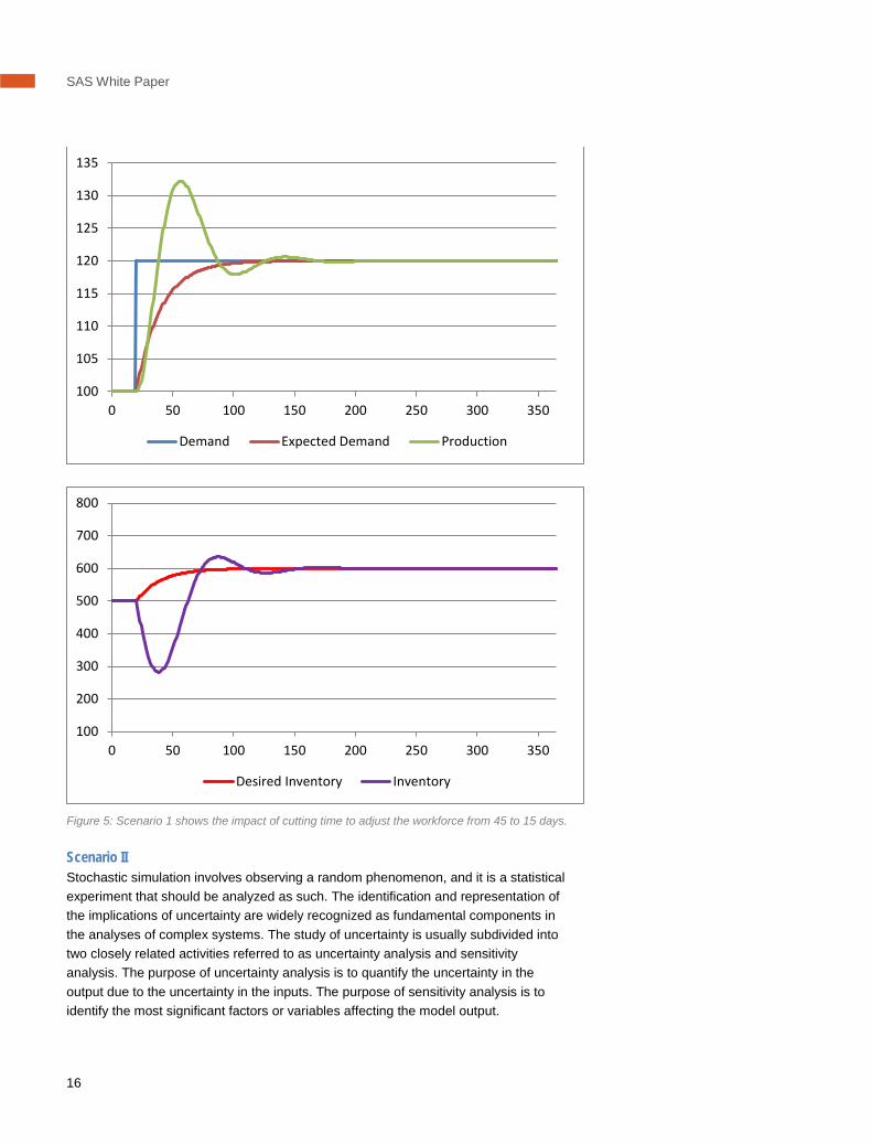
The next step is to display the uncertainty information contained in the mapping between inputs and model outputs. A good way to demonstrate the uncertainty is to estimate various summary statistics from the sample and also to show the distribution. For our output variable Inventory we have:

Figure 6: Density and summary statistics from MC simulation for production.

The standard deviation for Inventory is equal to approximately 158, which indicates that Inventory is not completely insensitive to the uncertainty carried from Demand and Productivity.

The final step is to study how the variation in Inventory can be apportioned to the two different sources of variation coming from Demand and Productivity. The technique we will use is known as a variance-based method. In particular, it is the Sobol sensitivity indices.12 The Sobol method involves a decomposition of the total variance of the model output in terms of increasing dimensionality. The variance decomposition underlying this approach is the same used in ANOVA-like decompositions of the variance.

Consider 𝑉(𝑌) to be the total variance of the model output from some function 𝑌 = 𝑓(𝑥1, … , 𝑥𝑘) where 𝑘 is the number of variables. Then this variance can be decomposed in terms of increasing dimensionality – i.e., the first-order effect is given by

𝑉𝑖 = 𝑉�𝑓𝑖(𝑋𝑖)� = 𝑉�𝐸(𝑌|𝑋𝑖)�,

12 (Sobol, 1993)


19

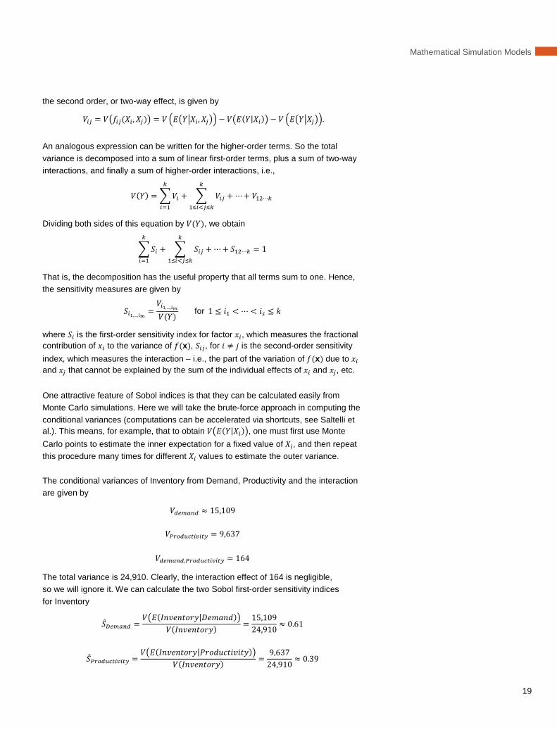
the second order, or two-way effect, is given by

𝑉𝑖𝑗 = 𝑉�𝑓𝑖𝑗(𝑋𝑖 ,𝑋𝑗)� = 𝑉 �𝐸�𝑌�𝑋𝑖 ,𝑋𝑗�� − 𝑉�𝐸(𝑌|𝑋𝑖)� − 𝑉 �𝐸�𝑌�𝑋𝑗��.

An analogous expression can be written for the higher-order terms. So the total variance is decomposed into a sum of linear first-order terms, plus a sum of two-way interactions, and finally a sum of higher-order interactions, i.e.,

𝑉(𝑌) = �𝑉𝑖 + � 𝑉𝑖𝑗 + ⋯+ 𝑉12⋯𝑘

𝑘

1≤𝑖<𝑗≤𝑘

𝑘

𝑖=1

Dividing both sides of this equation by 𝑉(𝑌), we obtain

�𝑆𝑖 + � 𝑆𝑖𝑗 + ⋯+ 𝑆12⋯𝑘

𝑘

1≤𝑖<𝑗≤𝑘

𝑘

𝑖=1

= 1

That is, the decomposition has the useful property that all terms sum to one. Hence, the sensitivity measures are given by

𝑆𝑖1,…,𝑖𝑚=𝑉𝑖1,…,𝑖𝑚

𝑉(𝑌) for 1 ≤ 𝑖1 < ⋯ < 𝑖𝑠 ≤ 𝑘

where 𝑆𝑖 is the first-order sensitivity index for factor 𝑥𝑖, which measures the fractional contribution of 𝑥𝑖 to the variance of 𝑓(x), 𝑆𝑖𝑗, for 𝑖 ≠ 𝑗 is the second-order sensitivity index, which measures the interaction – i.e., the part of the variation of 𝑓(x) due to 𝑥𝑖 and 𝑥𝑗 that cannot be explained by the sum of the individual effects of 𝑥𝑖 and 𝑥𝑗, etc.

One attractive feature of Sobol indices is that they can be calculated easily from Monte Carlo simulations. Here we will take the brute-force approach in computing the conditional variances (computations can be accelerated via shortcuts, see Saltelli et al.). This means, for example, that to obtain 𝑉�𝐸(𝑌|𝑋𝑖)�, one must first use Monte Carlo points to estimate the inner expectation for a fixed value of 𝑋𝑖, and then repeat this procedure many times for different 𝑋𝑖 values to estimate the outer variance.

The conditional variances of Inventory from Demand, Productivity and the interaction are given by

𝑉𝑑𝑒𝑚𝑎𝑛𝑑 ≈ 15,109

𝑉𝑃𝑟𝑜𝑑𝑢𝑐𝑡𝑖𝑣𝑖𝑡𝑦 = 9,637

𝑉𝑑𝑒𝑚𝑎𝑛𝑑,𝑃𝑟𝑜𝑑𝑢𝑐𝑡𝑖𝑣𝑖𝑡𝑦 = 164

The total variance is 24,910. Clearly, the interaction effect of 164 is negligible, so we will ignore it. We can calculate the two Sobol first-order sensitivity indices for Inventory

�̂�𝐷𝑒𝑚𝑎𝑛𝑑 =𝑉�𝐸(𝐼𝑛𝑣𝑒𝑛𝑡𝑜𝑟𝑦|𝐷𝑒𝑚𝑎𝑛𝑑)�

𝑉(𝐼𝑛𝑣𝑒𝑛𝑡𝑜𝑟𝑦) =15,10924,910 ≈ 0.61

�̂�𝑃𝑟𝑜𝑑𝑢𝑐𝑡𝑖𝑣𝑖𝑡𝑦 =𝑉�𝐸(𝐼𝑛𝑣𝑒𝑛𝑡𝑜𝑟𝑦|𝑃𝑟𝑜𝑑𝑢𝑐𝑡𝑖𝑣𝑖𝑡𝑦)�

𝑉(𝐼𝑛𝑣𝑒𝑛𝑡𝑜𝑟𝑦) =9,637

24,910 ≈ 0.39

SAS White Paper

20

With the uncertainty assertion imposed on Demand and Productivity through the normal distributions and parameters choices, the variance in Inventory can be reduced by demand control or shaping, if possible, and better production management.

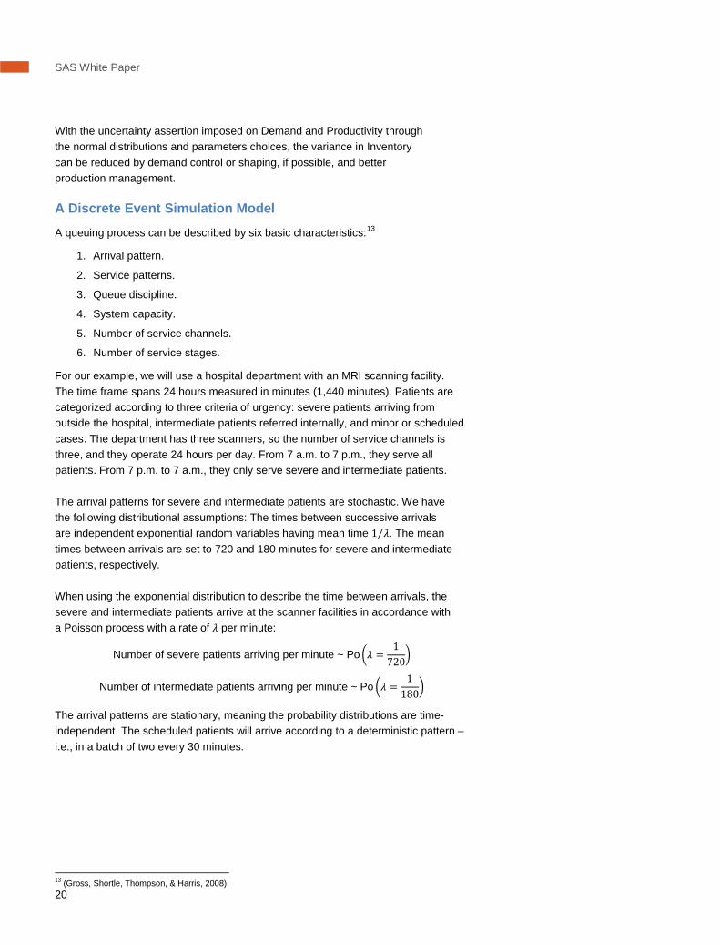
A Discrete Event Simulation Model

A queuing process can be described by six basic characteristics:13

1. Arrival pattern.

2. Service patterns.

3. Queue discipline.

4. System capacity.

5. Number of service channels.

6. Number of service stages.

For our example, we will use a hospital department with an MRI scanning facility. The time frame spans 24 hours measured in minutes (1,440 minutes). Patients are categorized according to three criteria of urgency: severe patients arriving from outside the hospital, intermediate patients referred internally, and minor or scheduled cases. The department has three scanners, so the number of service channels is three, and they operate 24 hours per day. From 7 a.m. to 7 p.m., they serve all patients. From 7 p.m. to 7 a.m., they only serve severe and intermediate patients.

The arrival patterns for severe and intermediate patients are stochastic. We have the following distributional assumptions: The times between successive arrivals are independent exponential random variables having mean time 1 𝜆⁄ . The mean times between arrivals are set to 720 and 180 minutes for severe and intermediate patients, respectively.

When using the exponential distribution to describe the time between arrivals, the severe and intermediate patients arrive at the scanner facilities in accordance with a Poisson process with a rate of 𝜆 per minute:

Number of severe patients arriving per minute ~ Po �𝜆 =1

720�

Number of intermediate patients arriving per minute ~ Po �𝜆 =1

180�

The arrival patterns are stationary, meaning the probability distributions are time-independent. The scheduled patients will arrive according to a deterministic pattern – i.e., in a batch of two every 30 minutes.

13 (Gross, Shortle, Thompson, & Harris, 2008)


21

The service pattern – i.e., the time used in the scanner by each patient – is also random. We will again assume that the probability distributions are time-independent. All service times follow a normal distribution:

Service time severe ~ N(120, 102)

Service time intermediate ~ N(60, 42)|

Service time scheduled ~ N(30, 22)

Before a severe or intermediate patient arrives at the scanner facility, the department will receive a warning that a nonscheduled patient will arrive, so it can clear and prepare the facility. The warning time – i.e., the time between the facility request and the patient’s actual arrival – will be uncertain. We assume that this time follows a normal distribution with mean equal to 25 and 20 minutes for severe and intermediate patients, respectively, and a small standard deviation of one in both cases.

The queue discipline, or the manner in which the three possible patient types are selected for scanning, are non-preemptive – i.e., the highest-priority patient goes to the front of the queue but cannot get into service until the patient presently there is completed, even though that patient has lower priority. Operationally, this means that when there is a request from a severe patient, the first available scanner will be made ready and kept vacant until the severe patient arrives.

The same procedure is followed with an intermediate patient. If a request for an intermediate patient is followed by a request for a severe patient before the scanner is occupied by the intermediate patient, the severe patient will enter the scanner before the intermediate patient because of higher priority. A pre-emptive queue discipline is where the lower-priority patient in service is pre-empted, and the scanning is stopped and then resumed after the higher-priority patient is served. However, this queue discipline is not practical in our system.

We do not assume any system capacity limitations, although in reality, there are obviously physical limitations to the number of patients who can be waiting. Scheduled patients can be on hold at their current locations until shortly before they can access the scanner. Therefore, no forced balk is necessary; all patients remain in the queue.

The human resource requirements for the three types of patient are as follows:

• Severe – one doctor and three nurses.

• Intermediate – one doctor and two nurses.

• Minor – one nurse.

SAS White Paper

22

The resources, together with the number of scanners, are the system constraints. If resources were unlimited – i.e., we had a large enough pool of scanners, doctors and nurses – all waiting times would be zero. We assume that both doctors and nurses are available during the entire simulation horizon of 1,440 minutes (24 hours). The available resources in the current system are:

• Three scanners.

• Two doctors.

• Five nurses.

We further assume that the queuing only has a single stage of service – e.g., we do not include a physical examination procedure before entering the scanner facility. In a system with more stages, both feedback and delay may occur. Figure 7 shows a graphical representation of the model developed in SAS Simulation Studio.

Figure 7: The model in SAS Simulation Studio.

The metric we want to study to assess the system is the average waiting time for three categories of patients and the percentage of patients that wait more than some desired level for service. The hospital’s goal is to have the average wait times for severe patients and intermediate patients be less than two minutes; the goal for scheduled patients is a wait of no more than 8 minutes. The management also has a goal that only 1 percent of severe and intermediate patients have the risk of waiting more than five minutes, and only 5 percent of scheduled patients will wait more than 15 minutes.


23

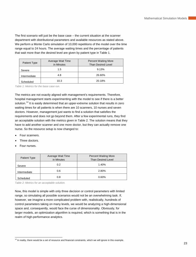
The first scenario will just be the base case – the current situation at the scanner department with distributional parameters and available resources as stated above. We perform a Monte Carlo simulation of 10,000 repetitions of the model over the time range equal to 24 hours. The average waiting times and the percentage of patients that wait more than the desired level are given by patient type in Table 1.

Patient Type Average Wait Time

in Minutes Percent Waiting More Than Desired Level

Severe 1.5 9.13%

Intermediate 4.8 26.60%

Scheduled 10.3 20.18%

Table 1: Metrics for the base case run.

The metrics are not exactly aligned with management’s requirements. Therefore, hospital management starts experimenting with the model to see if there is a better solution.14 It is easily determined that an upper-extreme solution that results in zero waiting times for all patients is when there are 10 scanners, 10 nurses and seven doctors. However, management just wants to find a solution that satisfies the requirements and does not go beyond them. After a few experimental runs, they find an acceptable solution with the metrics given in Table 2. The solution means that they have to add another scanner and one more doctor, but they can actually remove one nurse. So the resource setup is now changed to:

• Four scanners.

• Three doctors.

• Four nurses.

Patient Type Average Wait Time

in Minutes Percent Waiting More Than Desired Level

Severe 0.2 1.40%

Intermediate 0.6 2.80%

Scheduled 0.8 0.60%

Table 2: Metrics for an acceptable solution.

Now, this model is simple with only three decision or control parameters with limited range, so simulating all possible scenarios would not be an overwhelming task. If, however, we imagine a more complicated problem with, realistically, hundreds of control parameters taking on many levels, we would be analyzing a high-dimensional space and, consequently, would face the curse of dimensionality. Obviously, for larger models, an optimization algorithm is required, which is something that is in the realm of high-performance analytics.

14 In reality, there would be a set of resource and financial constraints, which we will ignore in this example.

SAS White Paper

24

Conclusion All decisions are based on expert knowledge and experience, and the challenge today is the vast amount of information or data needed to make efficient decisions every day under uncertainty. Gathering the overall picture in a simulation model enables a management team to comprehend such challenges.

Because it often is not possible, cost-effective or ethically correct to perform real experiments on complex physical systems, modeling and simulation are often employed to imitate and investigate how these systems and artifacts actually work. Simulation models can be used to investigate the intimate relationship that exists between the structure and behavior of dynamical systems – that is, how problematic behavior arises from the underlying system structure – and how the structure can then be modified and optimized to minimize or completely remove any deficiencies. The analysis brings the ability to draw conclusions, verify and validate any prespecified hypotheses, and make recommendations based on various simulations of the model.

Simulations provide critical input into most dynamic problems, including:

• Factory scheduling and manufacturing.

• Complex social, managerial, economic, defense or ecological systems.

• Financial prediction.

• Demand and supply chain planning.

• Market analysis.

• Customer service fulfillments (queuing systems).

Simulation can benefit literally any dynamical system characterized by interdependence, mutual interaction, information feedback and circular causality. After all, the success of a business is rarely the outcome of a random process. The high achievers are those who most effectively combine, manage and implement company goals, a competitive environment and resources through commitment, steadiness and determination. While having a solid covert strategy has always been important to the success of a company, having an effective overall analytical strategy – one that includes the consistent use of simulation, prediction and optimization – is rapidly becoming imperative for creating a strategic advantage.


25

References Arthur Andersen Business Consulting. (2000). Course Notes: System Dynamics.

De Geus, A. P. (1988). Planning as Learning. Harvard Business Review, 66(2).

Grant, R. M. (2010). Contemporary Strategy Analysis. Barcelona: Wiley.

Gross, D., Shortle, J. F., Thompson, J. M., & Harris, C. M. (2008). Fundamentals of Queueing Theory (4th Edition ed.). Wiley.

Halmos, P. R. (2006). Lectures on Ergodic Theory. New York: Chelsea Publishing Company.

Hamel, G., & Prahalad, C. K. (1994). Competing for the Future. Cambridge, MA: Harvard Business School Press.

Helton, J. C. (1993). Uncertainty and Sensitivity Analysis Techniques for Use in Performance Assessment. Reliability Engineering and System Safety, 42.

Katok, A., & Hasselblatt, B. (1996). Introduction to the Modern Theory of Dynamical Systems. New York: Cambridge University Press.

Larsen, E. R. (2002). Understanding and Using Scenarios:The Why, When and How of Scenarios. Teaching note.

Makridakis, S., Wheelwright, S., & Hyndman, R. (1998). Forecasting: Methods and Applications. New York: Wiley.

Nelson, B. L. (2010). Optimization via Simulation Over Discrete Decision Variables. Informs.

Oster, S. M. (1999). Modern Competitive Analysis. New York: Oxford University Press.

Porter, M. (1998). Competitive Advantage: Creating and Sustaining Superior Performance. Free Press.

Schmidt, J. W., & Taylor, R. E. (1970). Simualtion and Analysis of Industrial Systems. Homewood.

Sobol, I. M. (1993). Sensitivity Analysis for Nonlinear Mathematical Models. Mathematical Modeling and Computational Experiments, 14.

Sterman, J. D. (1989). Modeling Managerial Behavior: Misperceptions of Feedback in a Dynamic Decision Making Experiment. Management Science, 35.

Sterman, J. D. (2000). Business Dynamics: Systems Thinking and Modeling for a Complex World. Boston: McGraw-Hill.

Wack, P. (1985). Scenarios: Uncharted Waters Ahead. Harvard Business Review, 63(5).

Zeigler, B. P., Praehofer, H., & Kim, T. G. (2000). Theory of Modeling and Simulation. Academic Press.

SAS White Paper

26

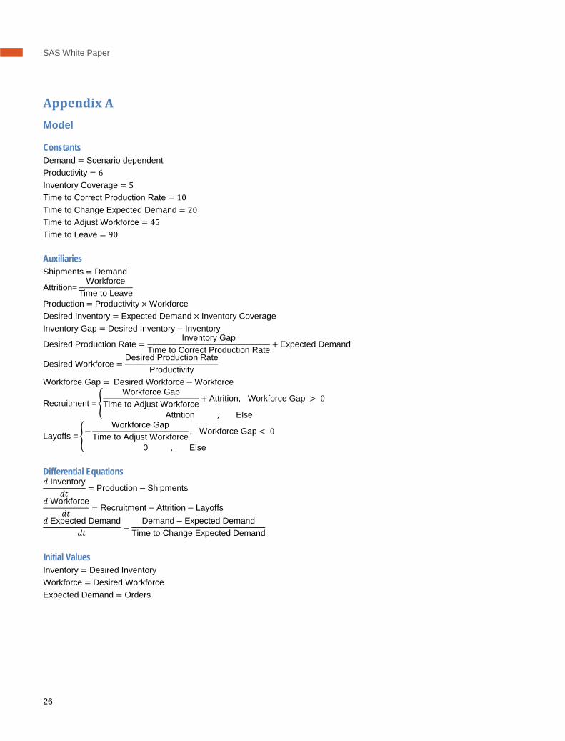
Appendix A Model

Constants Demand = Scenario dependent Productivity = 6 Inventory Coverage = 5 Time to Correct Production Rate = 10 Time to Change Expected Demand = 20 Time to Adjust Workforce = 45 Time to Leave = 90

Auxiliaries Shipments = Demand

Attrition=Workforce

Time to Leave

Production = Productivity × Workforce Desired Inventory = Expected Demand × Inventory Coverage Inventory Gap = Desired Inventory− Inventory

Desired Production Rate =Inventory Gap

Time to Correct Production Rate+ Expected Demand

Desired Workforce =Desired Production Rate

Productivity

Workforce Gap = Desired Workforce− Workforce

Recruitment =�Workforce Gap

Time to Adjust Workforce+ Attrition, Workforce Gap > 0

Attrition , Else

Layoffs =�−Workforce Gap

Time to Adjust Workforce, Workforce Gap < 0

0 , Else

Differential Equations 𝑑 Inventory

𝑑𝑡 = Production− Shipments 𝑑 Workforce

𝑑𝑡= Recruitment− Attrition− Layoffs

𝑑 Expected Demand𝑑𝑡 =

Demand− Expected DemandTime to Change Expected Demand

Initial Values Inventory = Desired Inventory Workforce = Desired Workforce Expected Demand = Orders


27

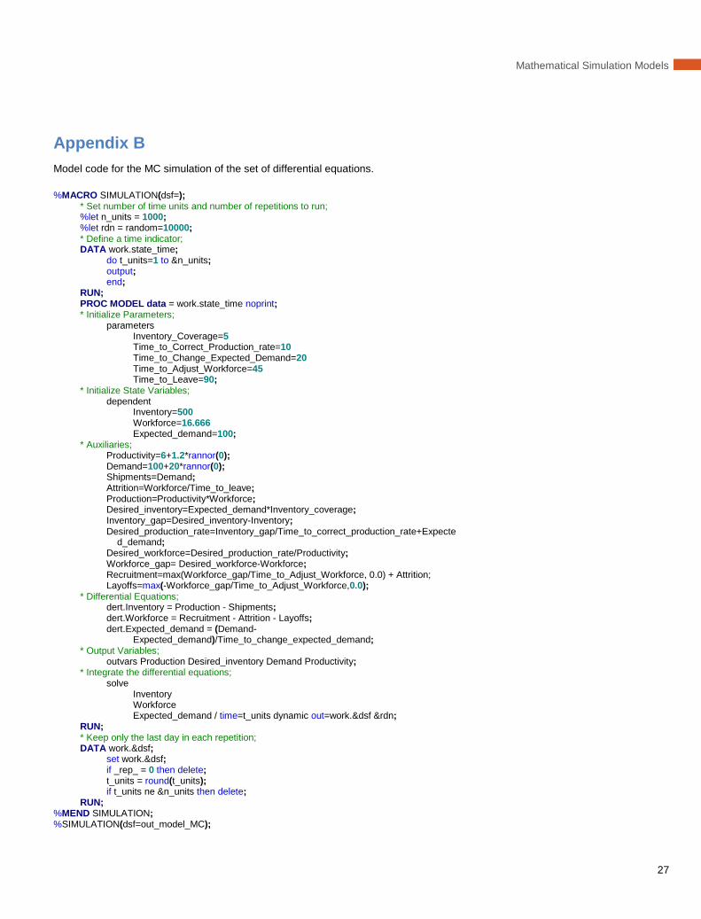
Appendix B Model code for the MC simulation of the set of differential equations.

%MACRO SIMULATION(dsf=); * Set number of time units and number of repetitions to run; %let n_units = 1000; %let rdn = random=10000; * Define a time indicator; DATA work.state_time; do t_units=1 to &n_units; output; end; RUN; PROC MODEL data = work.state_time noprint; * Initialize Parameters; parameters Inventory_Coverage=5 Time_to_Correct_Production_rate=10 Time_to_Change_Expected_Demand=20 Time_to_Adjust_Workforce=45 Time_to_Leave=90; * Initialize State Variables; dependent Inventory=500 Workforce=16.666 Expected_demand=100; * Auxiliaries; Productivity=6+1.2*rannor(0); Demand=100+20*rannor(0); Shipments=Demand; Attrition=Workforce/Time_to_leave; Production=Productivity*Workforce; Desired_inventory=Expected_demand*Inventory_coverage; Inventory_gap=Desired_inventory-Inventory;

Desired_production_rate=Inventory_gap/Time_to_correct_production_rate+Expected_demand;

Desired_workforce=Desired_production_rate/Productivity; Workforce_gap= Desired_workforce-Workforce;

Recruitment=max(Workforce_gap/Time_to_Adjust_Workforce, 0.0) + Attrition; Layoffs=max(-Workforce_gap/Time_to_Adjust_Workforce,0.0); * Differential Equations; dert.Inventory = Production - Shipments; dert.Workforce = Recruitment - Attrition - Layoffs; dert.Expected_demand = (Demand-

Expected_demand)/Time_to_change_expected_demand; * Output Variables; outvars Production Desired_inventory Demand Productivity; * Integrate the differential equations; solve Inventory Workforce Expected_demand / time=t_units dynamic out=work.&dsf &rdn; RUN; * Keep only the last day in each repetition; DATA work.&dsf; set work.&dsf; if _rep_ = 0 then delete; t_units = round(t_units); if t_units ne &n_units then delete; RUN; %MEND SIMULATION; %SIMULATION(dsf=out_model_MC);

SAS White Paper

28

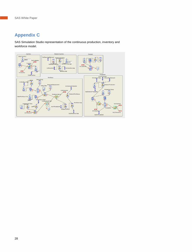
Appendix C SAS Simulation Studio representation of the continuous production, inventory and workforce model.

SAS Institute Inc. World Headquarters +1 919 677 8000To contact your local SAS office, please visit: sas.com/offices

SAS and all other SAS Institute Inc. product or service names are registered trademarks or trademarks of SAS Institute Inc. in the USA and other countries. ® indicates USA registration. Other brand and product names are trademarks of their respective companies. Copyright © 2012, SAS Institute Inc. All rights reserved. 105971_S91334_1012

About SASSAS is the leader in business analytics software and services, and the largest independent vendor in the business intelligence market. Through innovative solutions, SAS helps customers at more than 60,000 sites improve performance and deliver value by making better decisions faster. Since 1976 SAS has been giving customers around the world THE POWER TO KNOW®. For more information on SAS® Business Analytics software and services, visit sas.com.

http://www.sas.com/offices

http://www.sas.com

modeling and understanding the time evolution of real ... · modeling and understanding the time...

Documents