modeling and simulation of variable mass, flexible …...modeling and simulation of variable mass,...

Modeling and Simulation of Variable Mass, Flexible Structures

Patrick Tobbe, Alex Matras, Heath Wilson – Dynamic Concepts, Inc.

The advent of the new Ares I launch vehicle has highlighted the need for advanced dynamic analysis tools for variable mass, flexible structures. This system is composed of interconnected flexible stages or components undergoing rapid mass depletion through the consumption of solid or liquid propellant. In addition to large rigid body configuration changes, the system simultaneously experiences elastic deformations. In most applications, the elastic deformations are compatible with linear strain-displacement relationships and are typically modeled using the assumed modes technique. The deformation of the system is approximated through the linear combination of the products of spatial shape functions and generalized time coordinates. Spatial shape functions are traditionally composed of normal mode shapes of the system or even constraint modes and static deformations derived from finite element models of the system. Equations of motion for systems undergoing coupled large rigid body motion and elastic deformation have previously been derived through a number of techniques [1]. However, in these derivations, the mode shapes or spatial shape functions of the system components were considered constant. But with the Ares I vehicle, the structural characteristics of the system are changing with the mass of the system.

Previous approaches to solving this problem involve periodic updates to the spatial shape functions or interpolation between shape functions based on system mass or elapsed mission time. These solutions often introduce misleading or even unstable numerical transients into the system. Plus, interpolation on a shape function is not intuitive. This paper presents an approach in which the shape functions are held constant and operate on the changing mass and stiffness matrices of the vehicle components. Each vehicle stage or component finite element model is broken into dry structure and propellant models. A library of propellant models is used to describe the distribution of mass in the fuel tank or Solid Rocket Booster (SRB) case for various propellant levels. Based on the mass consumed by the liquid engine or SRB, the appropriate propellant model is coupled with the dry structure model for the stage. Then using vehicle configuration data, the integrated vehicle model is assembled and operated on by the constant system shape functions. The system mode shapes and frequencies can then be computed from the resulting generalized mass and stiffness matrices for that mass configuration. The rigid body mass properties of the vehicle are derived from the integrated vehicle model. The coupling terms between the vehicle rigid body motion and elastic deformation are also updated from the constant system shape functions and the integrated vehicle model. This approach was first used to analyze variable mass spinning beams and then prototyped into a generic dynamics simulation engine. The resulting code was tested against Crew Launch Vehicle (CLV-)class problems worked in the TREETOPS simulation package and by Wilson [2].

The Ares I System Integration Laboratory (SIL) is currently being developed at the Marshall Space Flight Center (MSFC) to test vehicle avionics hardware and software in a hardware-in-the-loop (HWIL) environment and certify that the integrated system is prepared for flight. The Ares I SIL utilizes the Ares Real-Time Environment for Modeling, Integration, and Simulation (ARTEMIS) tool to simulate the launch vehicle

https://ntrs.nasa.gov/search.jsp?R=20090036305 2020-04-27T02:25:52+00:00Z

and stimulate avionics hardware. Due to the presence of vehicle control system filters and the thrust oscillation suppression system, which are tuned to the structural characteristics of the vehicle, ARTEMIS must incorporate accurate structural models of the Ares I launch vehicle. The ARTEMIS core dynamics simulation models the highly coupled nature of the vehicle flexible body dynamics, propellant slosh, and vehicle nozzle inertia effects combined with mass and flexible body properties that vary significantly with time during the flight. All forces that act on the vehicle during flight must be simulated, including deflected engine thrust force, spatially distributed aerodynamic forces, gravity, and reaction control jet thrust forces. These forces are used to excite an integrated flexible vehicle, slosh, and nozzle dynamics model for the vehicle stack that simulates large rigid body translations and rotations along with small elastic deformations. Highly effective matrix math operations on a distributed, threaded high-performance simulation node allow ARTEMIS to retain up to 30 modes of flex for real-time simulation. Stage elements that separate from the stack during flight are propagated as independent rigid six degrees of freedom (6DOF) bodies. This paper will present the formulation of the resulting equations of motion, solutions to example problems, and describe the resulting dynamics simulation engine within ARTEMIS.

American Institute of Aeronautics and Astronautics1


Patrick A. Tobbe, Ph. D.1, Alex L. Matras, Ph. D.2, and Heath E. Wilson2

Dynamic Concepts, Inc., Huntsville, AL, 35806

The advent of the new Ares I launch vehicle has highlighted the need for advanced dynamics analysis tools for variable mass, flexible structures. Traditional flexible body simulation tools are based on the assumed modes technique in which component modes are constant. However, for variable mass systems, component and system modes vary with mass. This paper presents a technique that accurately simulates the response of a variable mass, flexible body while utilizing a constant set of shape functions. The approach allows for continued use of current flexible body simulation dynamics engines. The Ares Real-Time Environment for Modeling, Integration, and Simulation (ARTEMIS) has been developed for use by the Ares I launch vehicle System Integration Laboratory at the Marshall Space Flight Center. ARTEMIS utilizes the proposed approach in a real-time environment. Variable mass, flexible body test cases will be solved and presented from ARTEMIS and the multibody simulation tool TREETOPS.

Nomenclaturef0

α = force and moment vector for component αK0 = block diagonal of all component stiffness matricesk0

α = stiffness matrixM0 = block diagonal of all component mass matricesm0

α = mass matrix for component αipm = propellant mass flow rate for ith engine/thruster on component

mct = propellant mass consumed for tth tank on component

Md = dry component structural mass matrixMp = component propellant structural mass matrixM = component mass matrixq = state vector of constrained systemS = constraint matrixT10 = transformation to sort dependent and independent degrees of freedom orderu0

α = state vector in arbitrary order for component αu0 = state vector in arbitrary orderu1 = state vector sorted into dependent and independent degrees of freedomV = product of transformation, constraint and mode shape matricesvα = submatrix of V, partitioned to size of component αΓ0 = first mass integralΓ1 = second mass integralκ = generalized stiffness matrixμ = generalized mass matrixΦ = mode shape matrix

1 Chief Engineer, 6700 Odyssey Drive, Suite 202, AIAA member2 Engineer/Scientist, Simulation, Model, and Test Division, 6700 Odyssey Drive, Suite 202, AIAA member


I. Introductionnnovative dynamics analysis tools are essential for modeling and simulation of variable mass, flexible structures such as the new Ares I launch vehicle. This system is composed of interconnected flexible stages or components

undergoing rapid mass depletion through the consumption of solid or liquid propellant. In addition to large rigid body configuration changes, the system simultaneously experiences elastic deformations. In most applications, the elastic deformations are compatible with linear strain-displacement relationships and are typically modeled using the assumed modes technique. The deformation of the system is approximated through the linear combination of the products of spatial shape functions and generalized time coordinates. Spatial shape functions are traditionally composed of normal mode shapes of the system or even constraint modes and static deformations derived from finite element models of the system. Equations of motion for systems undergoing coupled large rigid body motion and elastic deformation have previously been derived through a number of techniques1. In these derivations, the mode shapes or spatial shape functions of the system components were considered constant; however, the structural characteristics of the Ares I vehicle change with the mass of the system.

Previous approaches to solving this problem involve periodic updates to the spatial shape functions or interpolation between shape functions based on system mass or elapsed mission time. The effects of these techniques have been studied2. These solutions often introduce misleading or even unstable numerical transients into the system. Plus, interpolation on a shape function is not intuitive. This paper presents an approach in which the shape functions are held constant and operate on the changing mass and stiffness matrices of the vehicle components. Each vehicle stage or component finite element model is broken into dry structure and propellant models. A library of propellant models is used to describe the distribution of mass in the fuel tanks or Solid Rocket Booster (SRB) for various propellant levels. Based on the mass consumed by the liquid engine or SRB, the appropriate propellant model is coupled with the dry structure model for the stage. Then, using vehicle configuration data, the integrated vehicle model is assembled and operated on by the constant system shape functions. The rigid body mass properties of the vehicle are derived from the integrated vehicle model. The coupling terms between the vehicle rigid body motion and elastic deformation are also updated from the constant system shape functions and the integrated vehicle model. This approach was first used to analyze variable mass spinning beams and then prototyped into a generic dynamics simulation engine. The resulting code was tested against Crew Launch Vehicle (CLV) class problems worked in the TREETOPS3 simulation package.

The Ares I System Integration Laboratory (SIL) is currently being developed at the Marshall Space Flight Center(MSFC) to test vehicle avionics hardware and software in a hardware-in-the-loop (HWIL) environment and certify that the integrated system is prepared for flight. The Ares I SIL utilizes the Ares Real-Time Environment for Modeling, Integration, and Simulation (ARTEMIS) tool to simulate the launch vehicle and avionics hardware. Due to the presence of vehicle control system filters and the thrust oscillation suppression system, which are tuned to the structural characteristics of the vehicle, ARTEMIS must incorporate accurate structural models of the Ares I launch vehicle. The ARTEMIS core dynamics simulation models the highly coupled nature of the vehicle flexible body dynamics, propellant slosh, and vehicle nozzle inertia effects combined with mass and flexible body properties that vary significantly with time during the flight. All forces that act on the vehicle during flight must be simulated, including deflected engine thrust force, spatially distributed aerodynamic forces, gravity, and reaction control jet thrust forces. These forces are used to excite an integrated flexible vehicle, slosh, and nozzle dynamics model for the vehicle stack that simulates large rigid body translations and rotations along with small elastic deformations. Cache optimized matrix math operations on a high-performance, multiprocessor, multi-node simulation computer allow ARTEMIS to achieve real-time while retaining up to 30 flexural modes. Stages that separate from the stack during flight are propagated as independent, rigid six degree of freedom (6DOF) bodies. This paper will present the formulation of the resulting equations of motion, solutions to example problems, and describe the resulting dynamics simulation engine within ARTEMIS.

II. Equations of Motion

The vehicle equations of motion, which constitute the dynamics engine of the ARTEMIS simulation, were derived using Boltzmann-Hamel equations1. Some of that derivation will be repeated here. Boltzmann-Hamel equations, often referred to as Lagrange's equations in quasi-coordinates, are a modified form of Lagrange's equations which operate in a moving reference frame. The elastic deformations of each body will be approximated using the assumed modes technique. This method is a popular technique for modeling structural flexibility in multi-body simulation packages. In this technique, the elastic deformation of each body is approximated through a linear

I


combination of the products of shape functions and generalized time coordinates. The shape functions are typically a subset of normal modes derived from a finite element model of the component.

Shown in Fig. 1 is a generic flexible body with vectors describing the position of the ith nodal body relative to inertial space O and a body fixed frame B. The nodal body has mass mi and an inertia tensor Ii. The location of the nodal body relative to the body fixed frame is denoted by i. In the deformed state of Fig. 2, the translational deformation of i relative to B is i and the rotational deformation is i. These deformations are assumed to be small,

as well as compatible with linear strain-displacement relations. The deformed nodal body position is

iii Rr (1)

The inertial translational velocity of point i is

iiii Rr (2)

Figure 2. Deformed Flexible Body

Figure 1. Undeformed Flexible Body


where is the angular velocity of the body frame B and i

is the time rate of change of the deformation relative to B. The kinetic energy of the system can be written as

iii

Tiiii IrrmT

21

21 (3)

The system potential energy is the strain energy resulting from body deformations. It can be computed from a finite element stiffness matrix of the structure as

tqKV TT

,21*

(4)

where K is the stiffness matrix, and are the nodal displacements, (q,t) are the system constraint equations, and is the array of Lagrange multipliers. The nodal displacements can be approximated using the assumed modes technique as

j

jiji (5)

and

jj

iji (6)

where ij and ij are the jth shape functions or modes at node i and j is the associated generalized coordinate. This is essentially a coordinate transformation from the finite element nodal displacements to a set of modal coordinates. The model is reduced in size by truncating the number of modes or shape functions used in the coordinate transformation. By inserting the energy expressions into Boltzmann-Hamel equations, the following equations of motion are derived.

Bkkjkjkj

BBBTBTki

Tii

Ti

Bj

BBBBB

BBBT

B

B

B

TT

T

TR

T

xT

IIIRTF

TIIRFRM

R

EII

BIIM

BI

I

22102

210

00

21

21

00

0

0

33

221~2

2

21

~

~0

(7)

The off axis terms in the system mass matrix of Eq. (7) are defined as

p

iijij m

10 (8)

p

iijiijiij Im

11 (9)


Tiijij

Ti

p

iij mI

11

1 (10)

p

iikijijk m

12 (11)

p

i

Tikijik

Tijijk mI

12 1 (12)

These terms are often referred to as the mass integrals and are a function of the rigid body mass properties and selected shape functions. Generally, Eqs. (8) through (12) are evaluated using shape functions and a finite element mass matrix. The mass integral terms couple the rigid body motion to the structural deformation as characterized by the shape functions. If the shape functions are orthogonal to the rigid body modes of the system, the mass integral terms defined by Eqs. (8) and (9) are zero. Typically the higher order terms of Eqs. (10), (11), and (12) are ignored except for extremely flexible systems. The system natural frequencies and mode shapes can be computed from the system mass matrix (coefficient matrix of the acceleration vector in the equations of motion) and the generalized stiffness matrix (augmented with rows and columns of zeroes for the rigid body degrees of freedom).

III. Variable MassThe changing structural characteristics of a variable mass system are difficult to model in a time domain

simulation. In the previous derivation of equations of motion, the shape functions were considered constant. In order to account for variations in the structural characteristics, the equations of motion could be expanded to include time-varying terms for the shape functions. However, time derivatives of the shape functions are difficult to compute or measure and add significantly to the numerical computations. Alternatively, different sets of mode shapes for each mass distribution can be processed before running the simulation. These sets can be periodically updated or interpolated during the simulation using Eq. (7), which introduces discontinuities in the vehicle deformations. Finally, a constant set of shape vectors that describe the bending characteristics of the vehicle for the entire propellant burn can be built from combinations of the mode shapes derived from different mass distributions. In this approach, the stage mass and stiffness matrices are combined to build the integrated vehicle mass and stiffness matrices in physical coordinates. The vehicle mass properties, mass integrals, and generalized mass and stiffness matrices are computed from the integrated vehicle mass and stiffness matrices and constant shape functions each time step and updated in Eq. (7). Through these updates, the system equations of motion reflect the current structural characteristics of the vehicle in a continuous manner while using a constant set of shape vectors.

Vehicles simulated by the ARTEMIS dynamics engine are decomposed into stages. Each stage is further subdivided into a dry substructure and propellant or tank substructures. Finite element models of each of the stage substructures are created and the mass and stiffness matrices extracted. Multiple propellant or tank models are constructed for various levels of propellant. Within ARTEMIS, the propellant consumed by each substructure is tracked through integration of mass flow rates and the corresponding mass and stiffness matrices are updated using interpolation. The mass and stiffness matrices for the stages and integrated vehicle are assembled through substructure coupling techniques, based on the appropriate vehicle configuration, and are used to calculate mass properties, mass integrals, and generalized mass and stiffness matrices. System shapes are selected off line to characterize the integrated vehicle flexibility for the appropriate configuration of stages. These shapes are orthogonalized with respect to the vehicle geometric rigid body modes to avoid singularities caused through dependencies with explicit rigid body degrees of freedom defined in Eq. (7). Mass properties are found through geometric rigid body modes operating on the system mass matrix. The process to update the vehicle properties based on propellant consumption in ARTEMIS is shown in Fig. 3 for parallel processing.


IV. Algorithm DescriptionThe primary goals of the implementation of these methods are to derive equations in forms that yield a minimal

number of run-time calculations, to parallelize tasks for efficient multithreading, and to design structures and algorithms to utilize the CPU cache as efficiently as possible.

The main technique used to reduce the number of run-time calculations is to partition the equations into terms that only need to be recomputed for a stage consuming mass, which is usually only one stage at a time. Additionally, the equations are written as a function of the individual stage mass and stiffness matrices before any transformations are applied. Thus, the equations reduce to simple matrix multiplications where most calculations may be performed one time at initialization and used for the duration of the simulation. The substructure coupling technique is particularly useful for deriving in this form.

A. Substructure CouplingSubstructure coupling is a convenient technique to assemble composite mass and stiffness matrices for structures

from individual components. This method, also known as Component Mode Synthesis, is described in detail by Craig4. The formulation presented here has been modified to account for multiple components and to provide for more efficient calculations.

Consider a set of components (stages or substructures) (α, β, γ, δ) where each component has a mass and stiffness matrix modeled by the following equation:

00000 fukum (13)

The subscript 0 represents an arbitrary DOF order. In this notation, the superscript represents the component (in this case). The state vector is represented by u, the mass matrix by m, the stiffness matrix by k, and the external force and moments by f.

In order to perform substructure coupling, the states must first be reordered into dependent and independent DOFs with a transformation matrix, T10, to compute the reordered state vector u1. Following Craig's approach, the constraint equations are applied to the system to generate a new, constrained state vector, q. These constraint equations take the form of a matrix multiplication.

Figure 3. Vehicle Properties Calculation


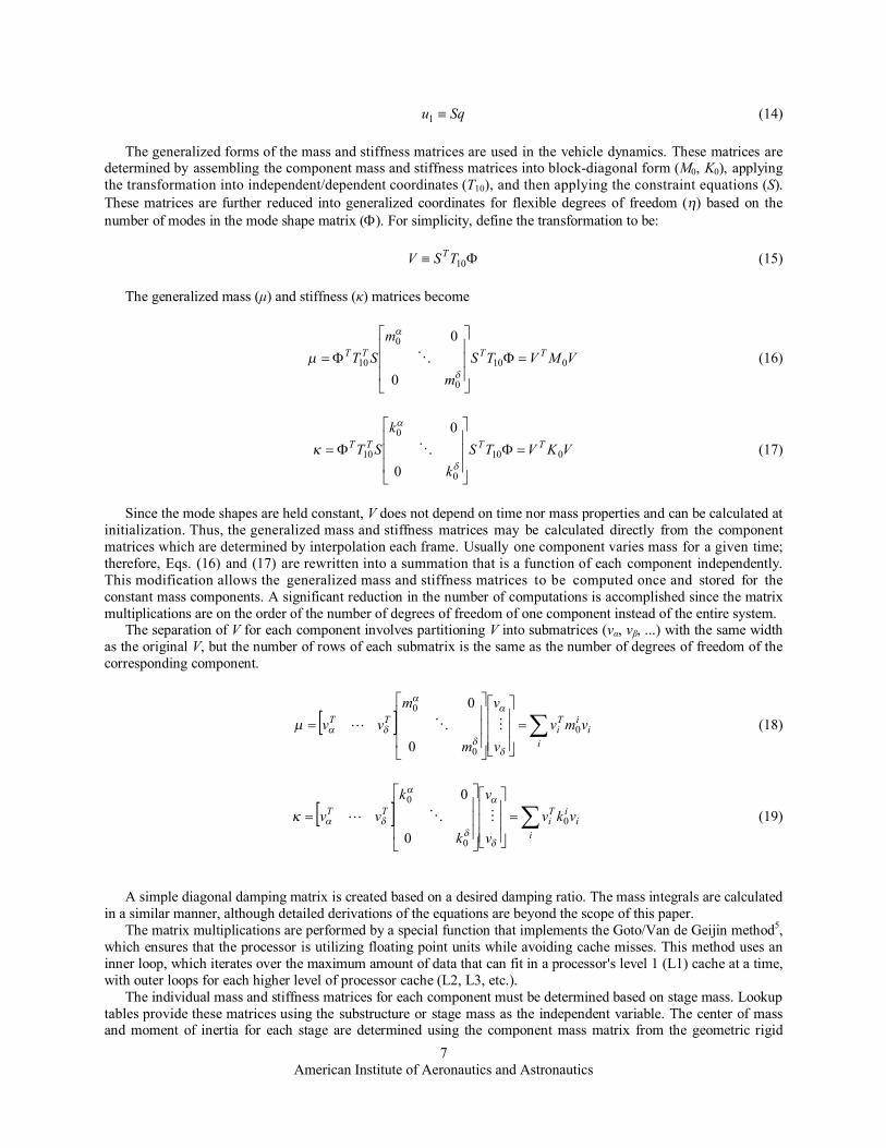
Squ 1 (14)

The generalized forms of the mass and stiffness matrices are used in the vehicle dynamics. These matrices are determined by assembling the component mass and stiffness matrices into block-diagonal form (M0, K0), applying the transformation into independent/dependent coordinates (T10), and then applying the constraint equations (S). These matrices are further reduced into generalized coordinates for flexible degrees of freedom () based on the number of modes in the mode shape matrix (). For simplicity, define the transformation to be:

10TSV T (15)

The generalized mass (μ) and stiffness (κ) matrices become

VMVTSm

mST TTTT

010

0

0

10

0

0

(16)

VKVTSk

kST TTTT

010

0

0

10

0

0

(17)

Since the mode shapes are held constant, V does not depend on time nor mass properties and can be calculated at initialization. Thus, the generalized mass and stiffness matrices may be calculated directly from the component matrices which are determined by interpolation each frame. Usually one component varies mass for a given time; therefore, Eqs. (16) and (17) are rewritten into a summation that is a function of each component independently. This modification allows the generalized mass and stiffness matrices to be computed once and stored for the constant mass components. A significant reduction in the number of computations is accomplished since the matrix multiplications are on the order of the number of degrees of freedom of one component instead of the entire system.

The separation of V for each component involves partitioning V into submatrices (vα, vβ, ...) with the same width as the original V, but the number of rows of each submatrix is the same as the number of degrees of freedom of the corresponding component.

i

iiT

iTT vmv

v

v

m

mvv 0

0

0

0

0

(18)

i

iiT

iTT vkv

v

v

k

kvv 0

0

0

0

0

(19)

A simple diagonal damping matrix is created based on a desired damping ratio. The mass integrals are calculated in a similar manner, although detailed derivations of the equations are beyond the scope of this paper.

The matrix multiplications are performed by a special function that implements the Goto/Van de Geijin method5, which ensures that the processor is utilizing floating point units while avoiding cache misses. This method uses an inner loop, which iterates over the maximum amount of data that can fit in a processor's level 1 (L1) cache at a time, with outer loops for each higher level of processor cache (L2, L3, etc.).

The individual mass and stiffness matrices for each component must be determined based on stage mass. Lookup tables provide these matrices using the substructure or stage mass as the independent variable. The center of mass and moment of inertia for each stage are determined using the component mass matrix from the geometric rigid


body modes technique. The center of mass and moment of inertia for the composite vehicle are calculated using the parallel axis theorem and the component mass properties.

B. MultithreadingThe algorithms for looking up the mass and stiffness matrices, calculating mass properties, and solving the

equations of motion have been designed to run on multi-core and multi-processor systems. Multi-threading of mass property and matrix calculations is straightforward since the calculations for each stage can be performed on a separate thread. Additionally, the mass integrals can be calculated on a separate thread.

The functions that solve the equations are separated into different tasks, which can be executed in parallel. Afunction (FApp) sums all the applied forces and moments (including force following terms) about the vehicle frame and calculates the generalized forces and moments. Another function (RHS) calculates the right hand side kinematic terms of Eq. (7). A third function calculates the system mass matrix and performs an LU decomposition. A fourth function performs the forward and backwards substitution (FBS) for the LU decomposed system mass matrix. Figure 4 illustrates a potential multithreading scheme. This scheme is based on using a separate thread for each stage and using separate threads for interpolating components and calculating generalized mass and stiffness matrices.

V. ExampleTo demonstrate the feasibility of this approach, an example problem was formulated and solved with the

simulation package TREETOPS. TREETOPS is a non-linear, multibody simulation tool which supports flexible bodies through the assumed modes technique. An example five-element beam, shown in Fig. 5, was constructed in NASTRAN and used as a model of dry structure.

Error!

Table 1 contains the properties for the dry beam. To simulate propellant, rigid bodies with mass and inertia were connected to each of the six nodes of the beam. The masses were depleted over time using a prescribed flow rate. A TREETOPS model was constructed with seven bodies. Body one was the dry flexible beam. Bodies two through seven represented the propellant nodal masses and inertias rigidly attached to the beam. The structural characteristics of body one were derived from the NASTRAN model of the dry beam.

Figure 4. Multithreading of ARTEMIS Dynamics

Figure 5. Flexible Beam Structure


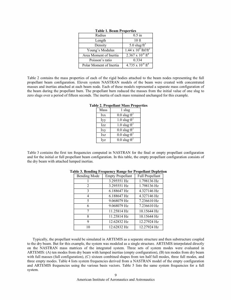
Table 2 contains the mass properties of each of the rigid bodies attached to the beam nodes representing the full propellant beam configuration. Eleven system NASTRAN models of the beam were created with concentrated masses and inertias attached at each beam node. Each of these models represented a separate mass configuration of the beam during the propellant burn. The propellant burn reduced the masses from the initial value of one slug to zero slugs over a period of fifteen seconds. The inertia of each mass remained unchanged for this example.

Table 3 contains the first ten frequencies computed in NASTRAN for the final or empty propellant configuration and for the initial or full propellant beam configuration. In this table, the empty propellant configuration consists of the dry beam with attached lumped inertias.

Typically, the propellant would be simulated in ARTEMIS as a separate structure and then substructure coupled to the dry beam. But for this example, the system was modeled as a single structure. ARTEMIS interpolated directly on the NASTRAN mass matrices of the integrated system. Three sets of system modes were evaluated in ARTEMIS: (A) ten modes from dry beam with lumped inertias (empty configuration), (B) ten modes from dry beam with full masses (full configuration), (C) sixteen combined shapes from ten half full modes, three full modes, and three empty modes. Table 4 lists system frequencies derived from a NASTRAN model of the empty configuration and ARTEMIS frequencies using the various basis vectors. Table 5 lists the same system frequencies for a full system.

Table 1. Beam PropertiesRadius 0.5 inLength 10 ftDensity 5.0 slug/ft3

Young’s Modulus 1.44 x 109 lbf/ft2

Area Moment of Inertia 2.367 x 10-6 ft4

Poisson’s ratio 0.334Polar Moment of Inertia 4.735 x 10-6 ft4

Table 3. Bending Frequency Range for Propellant DepletionBending Mode Empty Propellant Full Propellant

1 3.295551 Hz 1.798136 Hz2 3.295551 Hz 1.798136 Hz3 6.188647 Hz 4.327146 Hz4 6.188647 Hz 4.327146 Hz5 9.068079 Hz 7.236610 Hz6 9.068079 Hz 7.236610 Hz7 11.25814 Hz 10.15644 Hz8 11.25814 Hz 10.15644 Hz9 12.62832 Hz 12.27924 Hz10 12.62832 Hz 12.27924 Hz

Table 2. Propellant Mass PropertiesMass 1 slugIxx 0.0 slug·ft2

Iyy 1.0 slug·ft2

Izz 1.0 slug·ft2

Ixy 0.0 slug·ft2

Ixz 0.0 slug·ft2

Iyz 0.0 slug·ft2


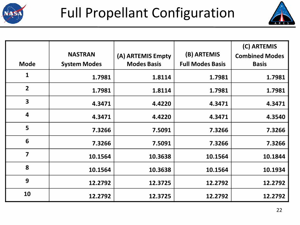
As seen in Tables 4 and 5, no single mode basis set works well for the full spectrum of propellant levels. However, at the computational expense of additional shapes, the combined set of vectors from various mass configurations performs well. Any screening or shape selection process should, as a minimum, evaluate the predicted system frequencies for the configurations being studied. Resulting system mode shapes also need to be considered.

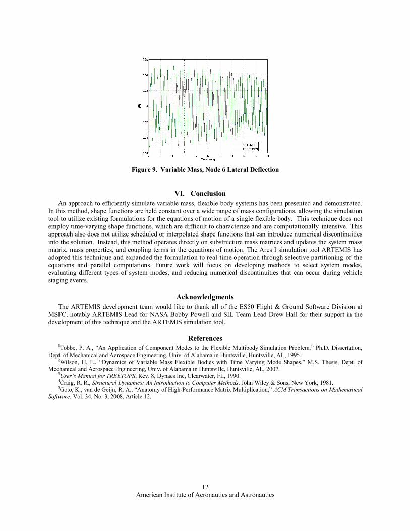
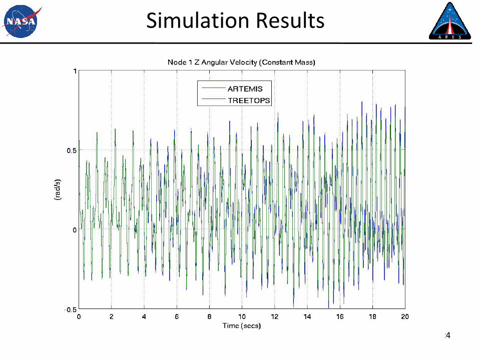
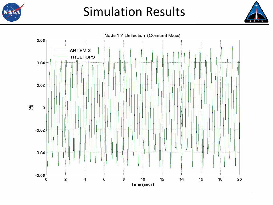
The simulations began with the system at rest. A 500-pound excitation force was applied along the beam Y-axis at node 1 for 0.004 seconds and then released. The simulation was run for constant mass and variable mass problems. Figure 6 depicts the angular velocity of node 1, including bending, and Fig. 7 contains the lateral deflection of node 6 for the full constant mass run. The results show excellent agreement between TREETOPS and ARTEMIS while using different dynamic formulations and support the verification of Eq. 7. Next, a variable mass case was run to evaluate the feasibility of the approach utilized in ARTEMIS and outlined in this paper. A 15 second burn with a burn rate of 1/15 slugs/second for each propellant mass started at 2 seconds. At the end of the burn, the propellant masses were completely depleted. The inertia of each of the propellant masses was not changed for this problem. Figure 8 is the angular velocity of node 1 and Fig. 9 is the lateral deflection of node 1. Again, there is excellent agreement between TREETOPS and ARTEMIS.

Table 5. Full System Frequencies

Mode

NASTRANSystem Modes

(A) ARTEMIS

Empty Modes

(B) ARTEMIS

Full Modes

(C) ARTEMISCombined

Modes1 1.7981 1.8114 1.7981 1.79812 1.7981 1.8114 1.7981 1.79813 4.3471 4.4220 4.3471 4.34714 4.3471 4.4220 4.3471 4.35405 7.3266 7.5091 7.3266 7.32666 7.3266 7.5091 7.3266 7.32667 10.1564 10.3638 10.1564 10.18448 10.1564 10.3638 10.1564 10.19349 12.2792 12.3725 12.2792 12.2792

10 12.2792 12.3725 12.2792 12.2792

Table 4. Empty System Frequencies

Mode

NASTRANSystem Modes

(A) ARTEMIS

Empty Modes

(B) ARTEMIS

Full Modes

(C) ARTEMISCombined

Modes1 3.2956 3.2956 3.3143 3.29562 3.2956 3.2956 3.3143 3.29563 6.1886 6.1886 6.2775 6.18864 6.1886 6.1886 6.2775 6.22825 9.0681 9.0681 9.3115 9.06816 9.0681 9.0681 9.3115 9.06817 11.2581 11.2581 11.5788 11.29498 11.2581 11.2581 11.5788 11.36589 12.6283 12.6283 12.7900 12.6283

10 12.6283 12.6283 12.7900 12.6283


Figure 6. Constant Mass, Node 1 Angular Velocity

Figure 7. Constant Mass, Node 6 Lateral Deflection

Figure 8. Variable Mass, Node 1 Angular Velocity


VI. ConclusionAn approach to efficiently simulate variable mass, flexible body systems has been presented and demonstrated.

In this method, shape functions are held constant over a wide range of mass configurations, allowing the simulation tool to utilize existing formulations for the equations of motion of a single flexible body. This technique does not employ time-varying shape functions, which are difficult to characterize and are computationally intensive. This approach also does not utilize scheduled or interpolated shape functions that can introduce numerical discontinuities into the solution. Instead, this method operates directly on substructure mass matrices and updates the system mass matrix, mass properties, and coupling terms in the equations of motion. The Ares I simulation tool ARTEMIS has adopted this technique and expanded the formulation to real-time operation through selective partitioning of the equations and parallel computations. Future work will focus on developing methods to select system modes, evaluating different types of system modes, and reducing numerical discontinuities that can occur during vehicle staging events.

AcknowledgmentsThe ARTEMIS development team would like to thank all of the ES50 Flight & Ground Software Division at

MSFC, notably ARTEMIS Lead for NASA Bobby Powell and SIL Team Lead Drew Hall for their support in the development of this technique and the ARTEMIS simulation tool.

References1Tobbe, P. A., “An Application of Component Modes to the Flexible Multibody Simulation Problem,” Ph.D. Dissertation,

Dept. of Mechanical and Aerospace Engineering, Univ. of Alabama in Huntsville, Huntsville, AL, 1995.2Wilson, H. E., “Dynamics of Variable Mass Flexible Bodies with Time Varying Mode Shapes.” M.S. Thesis, Dept. of

Mechanical and Aerospace Engineering, Univ. of Alabama in Huntsville, Huntsville, AL, 2007.3User’s Manual for TREETOPS, Rev. 8, Dynacs Inc, Clearwater, FL, 1990.4Craig, R. R., Structural Dynamics: An Introduction to Computer Methods, John Wiley & Sons, New York, 1981.5Goto, K., van de Geijn, R. A., “Anatomy of High-Performance Matrix Multiplication,” ACM Transactions on Mathematical

Software, Vol. 34, No. 3, 2008, Article 12.

Figure 9. Variable Mass, Node 6 Lateral Deflection

1


Patrick Tobbe, Ph. D.Alex Matras, Ph. D.

Heath WilsonDynamic Concepts, Inc.

Huntsville, Ala.

2

Outline

Equations of Motion of a Flexible Body

Variable Mass Challenge and Solutions

ARTEMIS Simulation Description

Implementation of Equations of Motion

Initial Validation Test Case

Results / Observations

Future Work

3

Equations of Motion for Flexible Body

Formulation to accurately simulate the response of a single vehicle

Derived using modified form of Boltzmann-Hamel equations• Energy method allowing kinetic and potential energies to

be expressed in coordinates in rotating frame

Structural flexibility of vehicles / bodies modeled using assumed modes technique

Equations of motion allow for large rigid body translations and rotations coupled with small body deformations

4

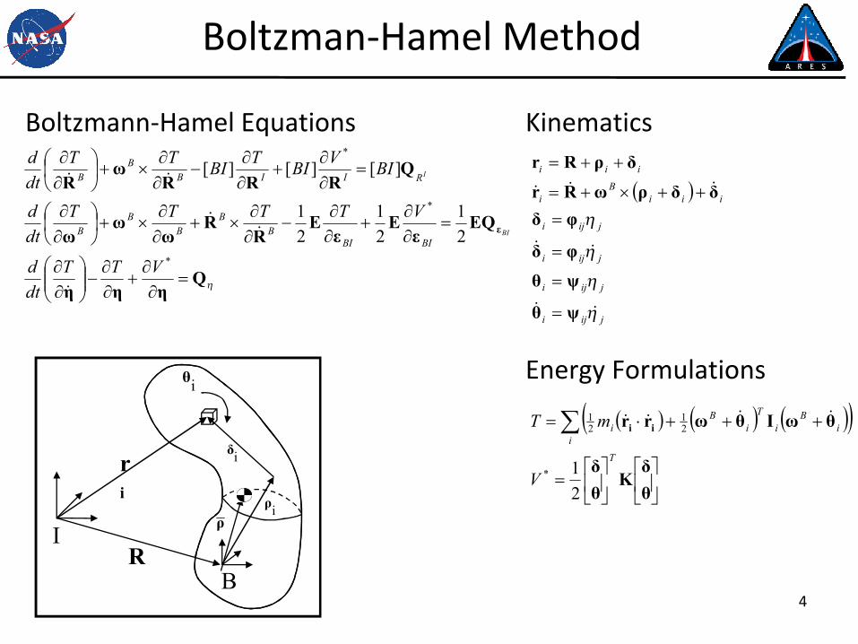
Boltzman-Hamel Method

Boltzmann-Hamel Equations Kinematics

Energy Formulations

Qηηη

EQε

Eε

ER

Rω

ωω

QRRR

ωR

ε

*

*

*

21

21

21

][][][

VTTdtd

VTTTTdtd

BIVBITBITTdtd

BI

I

BIBIB

BB

BB

RIIBB

B

B

I

ri

R

iθ

iδ

iρρ

θδ

Kθδ

θωIθωrr ii

Ti

iB

iT

iB

i

V

mT

21*

21

21

jiji

jiji

jiji

jiji

iiiB

i

iii

ψθ

ψθφδ

φδδδρωRr

δρRr

5

Equations of Motion

Bk

Tjkkjkj

BBBTi

Tii

Ti

Bkjkj

Tjkjkj

Tjj

BBkjjk

B

Bkj

Tjkjkj

TjjB

BB

BBBB

B

B

Tj

TTjkj

Tjkjkj

TjjB

x

ηηTF

ηηηηη

mηη

ηηη

mm

ηηηmmm

TωIIIωRωΓκηψφ

ωIIII

ρηΓωRΓηΓω

ωIIIIIωT

η2ΓηΓρωRωF

ηωR

μΓΓΓΓΓIIIIIρηΓ

ΓρηΓI

0

22121

0

2221

11

021

2221

11

00

21

212221

110

0033

2

)(

6

Mass Integrals

Mass integrals model coupling between rigid body and flex body dynamics

Using momentum arguments, developed ways of calculating these from mass matrices

Γ0 and Γ1 go to zero when mode shapes are orthogonal to mass matrix, the others are negligible• Not always the case using our approach

The Γ2, I1 & I2 mass integrals may be neglected for systems that do not undergo very large deformations (e.g. for the Ares I)

iikijijk

iijiijiij

iijij

m

m

m

φφΓ

ψIφρΓ

φΓ

2

1

0

i

Tikijx

Tijiijk

i

Tiijxijiij

m

m

φφIφρI

ρφIφρI

332

331

7

Equations of Motion

BBTi

Tii

Ti

BBBBB

BB

BBBB

B

B

TTB

x

TFm

mm

mmm

RωΓκηψφρηΓωRηΓωωIωT

η2ΓηΓρωRωF

ηωR

μΓΓΓIρηΓΓρηΓI

0

0

01

00

1

10

0033

)(

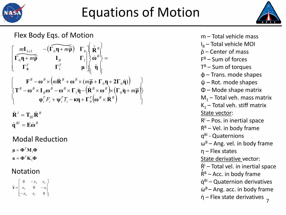
Flex Body Eqs. of Motion

BBI

BBI

I

ωEqRTR

Modal Reduction

ΦKΦκ

ΦMΦμ

1

1T

T

m – Total vehicle massIB – Total vehicle MOIρ – Center of massFB – Sum of forcesTB – Sum of torquesφ – Trans. mode shapesψ – Rot. mode shapesΦ – Mode shape matrix M1 – Total veh. mass matrixK1 – Total veh. stiff matrixState vector:RI – Pos. in inertial spaceRB – Vel. in body frameqBI - QuaternionsωB – Ang. vel. in body frameη – Flex statesState derivative vector:RI – Total vel. in inertial spaceRB – Acc. in body frameqBI – Quaternion derivativesωB – Ang. acc. in body frameη – Flex state derivatives

˙

˙

˙

˙

˙

˙

˚

¯

Notation

00

0~

12

13

23

xxxx

xxx

8

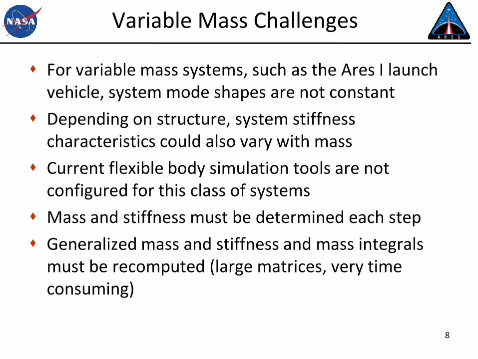
Variable Mass Challenges

For variable mass systems, such as the Ares I launch vehicle, system mode shapes are not constant

Depending on structure, system stiffness characteristics could also vary with mass

Current flexible body simulation tools are not configured for this class of systems

Mass and stiffness must be determined each step

Generalized mass and stiffness and mass integrals must be recomputed (large matrices, very time consuming)

9

Variable Mass Solutions

Schedule / interpolate new system shapes as a function of mass• Discontinuities in deformations at updates• Orthogonality of modes with respect to system mass and stiffness

matrices• Determining the rate to update modal data

Add time varying mode shape terms to derivation of EOM (Wilson)• Additional terms add significant computation time• Computing derivatives of mode shapes for vehicle configurations is

very difficult Hold shape functions constant between staging and vary

physical (FEM) mass and stiffness matrix (i.e. use Ritz vectors) Partition matrix equations by component, and only perform

calculations on parts which change

10

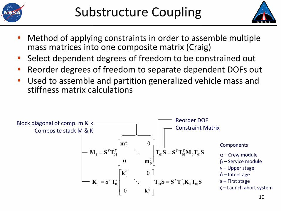
Substructure Coupling

Method of applying constraints in order to assemble multiple mass matrices into one composite matrix (Craig)

Select dependent degrees of freedom to be constrained out Reorder degrees of freedom to separate dependent DOFs out Used to assemble and partition generalized vehicle mass and

stiffness matrix calculations

Reorder DOFConstraint Matrix

Block diagonal of comp. m & kComposite stack M & K

STMTSSTm

mTSM 0100101

0

0

011

0

0TTTT

STKTSSTk

kTSK 0100101

0

0

011

0

0TTTT

Components

α – Crew moduleβ – Service moduleγ – Upper stageδ – Interstageε – First stageζ – Launch abort system

11

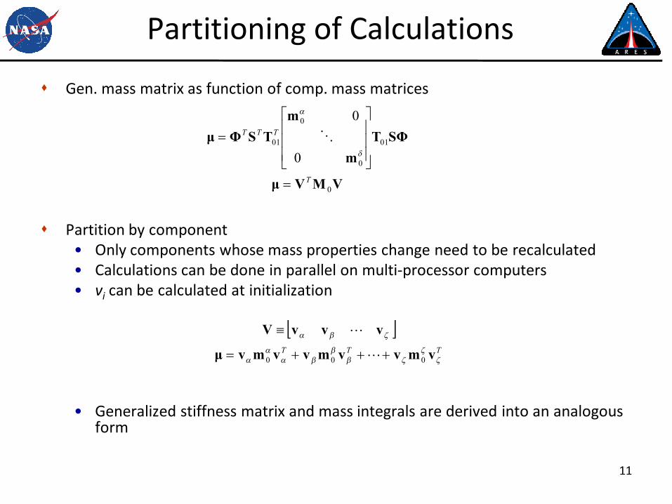
Partitioning of Calculations

Gen. mass matrix as function of comp. mass matrices

Partition by component• Only components whose mass properties change need to be recalculated• Calculations can be done in parallel on multi-processor computers• vi can be calculated at initialization

• Generalized stiffness matrix and mass integrals are derived into an analogous form

VMVμ

SΦTm

mTSΦμ

0

01

0

0

01

0

0

T

TTT

TTT

vmvvmvvmvμ

vvvV

000

12

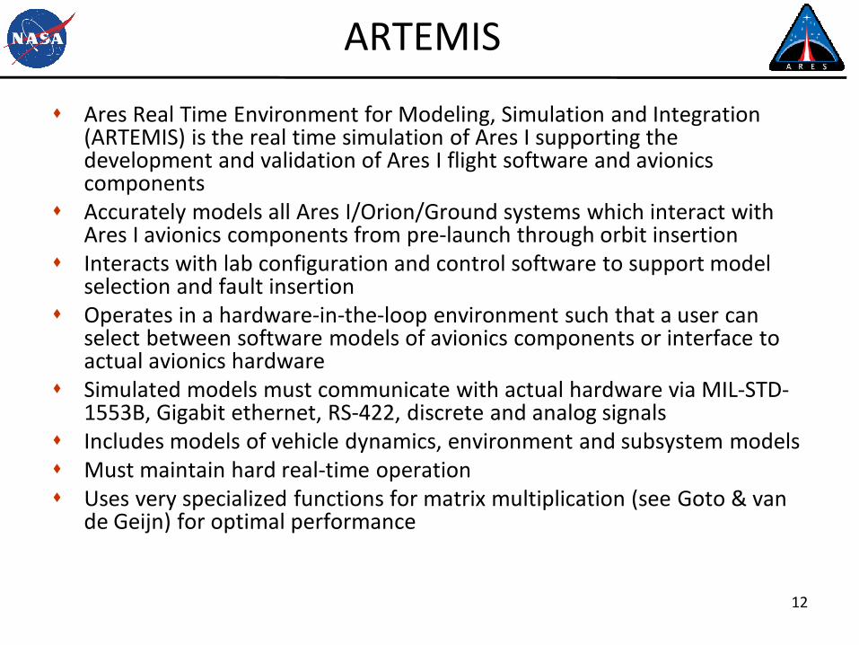
ARTEMIS

Ares Real Time Environment for Modeling, Simulation and Integration (ARTEMIS) is the real time simulation of Ares I supporting the development and validation of Ares I flight software and avionics components

Accurately models all Ares I/Orion/Ground systems which interact with Ares I avionics components from pre-launch through orbit insertion

Interacts with lab configuration and control software to support model selection and fault insertion

Operates in a hardware-in-the-loop environment such that a user can select between software models of avionics components or interface to actual avionics hardware

Simulated models must communicate with actual hardware via MIL-STD-1553B, Gigabit ethernet, RS-422, discrete and analog signals

Includes models of vehicle dynamics, environment and subsystem models Must maintain hard real-time operation Uses very specialized functions for matrix multiplication (see Goto & van

de Geijn) for optimal performance

13

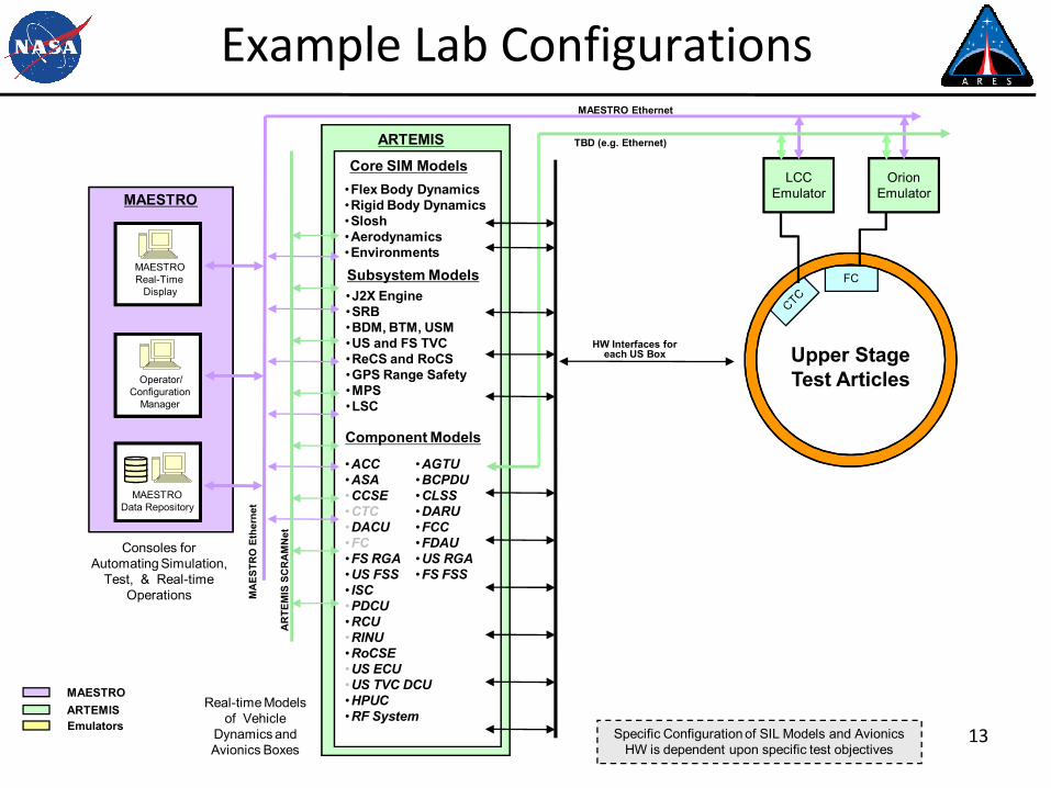
Example Lab Configurations

Core SIM Models

MAESTRO

MAESTROReal-Time

Display

MAESTROData Repository

Operator/Configuration

Manager

Consoles for Automating Simulation,

Test, & Real-time Operations

ARTEMIS

Real-time Models of Vehicle

Dynamics and Avionics Boxes

MAESTRO Ethernet

MAESTROARTEMISEmulators Specific Configuration of SIL Models and Avionics

HW is dependent upon specific test objectives

FC

LCCEmulator

OrionEmulator

Upper StageTest Articles

TBD (e.g. Ethernet)

HW Interfaces for each US Box

Component Models

Subsystem Models

•Flex Body Dynamics•Rigid Body Dynamics•Slosh•Aerodynamics•Environments

AR

TEM

IS S

CR

AM

Net

MA

ESTR

O E

ther

net

•ACC•ASA•CCSE•CTC•DACU•FC•FS RGA•US FSS• ISC•PDCU•RCU•RINU•RoCSE•US ECU•US TVC DCU•HPUC•RF System

•AGTU•BCPDU•CLSS•DARU•FCC•FDAU•US RGA•FS FSS

•J2X Engine•SRB•BDM, BTM, USM•US and FS TVC•ReCS and RoCS•GPS Range Safety•MPS•LSC

14

Example Lab Configurations

Core SIM Models

•ACC•ASA•CCSE•CTC•DACU•FC•FS RGA•US FSS• ISC•PDCU•RCU•RINU•RoCSE•US ECU•US TVC DCU•HPUC•RF System

MAESTRO

MAESTROReal-Time

Display

MAESTROData Repository

Operator/Configuration

Manager

Consoles for Automating Simulation,

Test, & Real-time Operations

ARTEMIS

Real-time Models of Vehicle

Dynamics and Avionics Boxes

MAESTRO Ethernet

MAESTROARTEMISEmulators Specific Configuration of SIL Models and Avionics HW is

dependent upon specific test objectives

FC

PD

CUR

INU

US ECU

LCCEmulator

OrionEmulator

Upper StageTest Articles

TBD (e.g. Ethernet)

HW Interfaces for each US Box

Component Models

Subsystem Models

•Flex Body Dynamics•Rigid Body Dynamics•Slosh•Aerodynamics•Environments

•J2X Engine•SRB•BDM, BTM, USM•US and FS TVC•ReCS and RoCS•GPS Range Safety•MPS•LSC

AR

TEM

IS S

CR

AM

Net

MA

ESTR

O E

ther

net

USA EGSE(Certified by

SITF/SIL))

•AGTU•BCPDU•CLSS•DARU•FCC•FDAU•US RGA•FS FSS

15

ARTEMIS Flexible Body Configuration

Define vehicle as a single body composed of components (stages) connected at nodes

Each component is composed of structure and propellant Component input data consists of FEM mass and stiffness matrices, DOF

map, and node geometry of structure and propellant Re-compute propellant mass and stiffness matrices each integration time

step via interpolation with respect to mass Update component mass properties using geometric rigid body modes

technique Assemble vehicle mass and stiffness matrices each integration time step

via automated substructure coupling Use linearly independent combination of vehicle mode shapes / Ritz

vectors computed from various mass configurations analyzed• Hold mode shapes or Ritz vectors constant

At staging event, update vehicle geometry, mass properties, Ritz vectors Spawn and propagate separated rigid vehicle (can be composed of

multiple cores or stages) based on flight phase

16

Ares I Flight Phases

USJ2-X

FSSRB

Innerstage

Instrument Unit

Crew ModuleService Module

LAS

las

las

cm

sm

us

is

fs

Nominal Flight Phases Abort PhasesNominal Flight Phases Abort Phases

17

Variable Mass, Flexible Body Test Case

Developed variable mass, flexible body example problem composed of dry beam structure augmented with propellant nodes

Applied sinusoidal force to end node of beam while depleting mass from propellant nodes

No modal damping Constructed 36 DOF FEM of dry beam Developed FEMs of dry beam and various levels of propellant Extracted mass and stiffness matrices from FEM for various

levels of propellant for use in ARTEMIS Computed system frequencies for empty and full propellant

levels to support Ritz vector selection in ARTEMIS Serves as validation for the implementation of flex body

dynamics in ARTEMIS

18

Test Case

Sinusoidal force applied in -Y direction at node 1 from time = 0 for 0.4 seconds with a magnitude of 10 pounds

Mass depletion rate of 1/15 slugs/second starting at time = 2 seconds until time = 17 seconds

x

y

Node 1 Node 2 Node 3 Node 4 Node 5 Node 6

19

ARTEMIS Configuration of Test Case

Configured ARTEMIS for a single, flexible body using constant set of system modes and library of system mass and stiffness matrices

Used three different sets of shapes in ARTEMIS : empty system, full system, and combination of empty and full systems

Computed system frequencies from ARTEMIS M and K for empty and full propellant levels, compared to system FEM modes

Applied prescribed forcing function to node 1 Computed total angular velocity of node 1 and

translational deflection of node 6 for constant mass and variable mass configurations

20

Test Case

Radius 0.5 in Mass 1.0 slug

Length 10 ft Ixx 0.0 slug·ft2

Density 5.0 slug/ft3 Iyy 1.0 slug·ft2

Young’s Modulus

1.44 x 109

lbf/ft2 Izz 1.0 slug·ft2

Area Moment of Inertia

2.367 x 10-6 ft4 Ixy 0.0 slug·ft2

Poisson’s ratio 0.334 Ixz 0.0 slug·ft2

Polar Moment of Inertia

4.735 x 10-6 ft4

21

FEM System Natural Frequencies

Bending Mode Empty Propellant Full Propellant

1 3.295551 Hz 1.798136 Hz

2 3.295551 Hz 1.798136 Hz

3 6.188647 Hz 4.327146 Hz

4 6.188647 Hz 4.327146 Hz

5 9.068079 Hz 7.236610 Hz

6 9.068079 Hz 7.236610 Hz

7 11.25814 Hz 10.15644 Hz

8 11.25814 Hz 10.15644 Hz

9 12.62832 Hz 12.27924 Hz

10 12.62832 Hz 12.27924 Hz

22

Full Propellant Configuration

Mode

NASTRAN

System Modes(A) ARTEMIS Empty

Modes Basis

(B) ARTEMIS

Full Modes Basis

(C) ARTEMIS

Combined Modes Basis

1 1.7981 1.8114 1.7981 1.7981

2 1.7981 1.8114 1.7981 1.7981

3 4.3471 4.4220 4.3471 4.3471

4 4.3471 4.4220 4.3471 4.3540

5 7.3266 7.5091 7.3266 7.3266

6 7.3266 7.5091 7.3266 7.3266

7 10.1564 10.3638 10.1564 10.1844

8 10.1564 10.3638 10.1564 10.1934

9 12.2792 12.3725 12.2792 12.2792

10 12.2792 12.3725 12.2792 12.2792

23

TREETOPS Configuration for Test Case

TREETOPS is a multibody simulation package developed at the Marshall Spaceflight Center that supports flexible bodies

Built TREETOPS simulation of dry flexible beam (body 1) rigidly attached to propellant masses (bodies 2 through 7)

Described structural flexibility of body 1 through dry beam modes

Applied prescribed forcing function to node 1 Computed total angular velocity of node 1 and

translational deflection of node 6 for constant mass and variable mass configurations

24

Simulation Results

25

Simulation Results

26

Simulation Results

27

Simulation Results

28

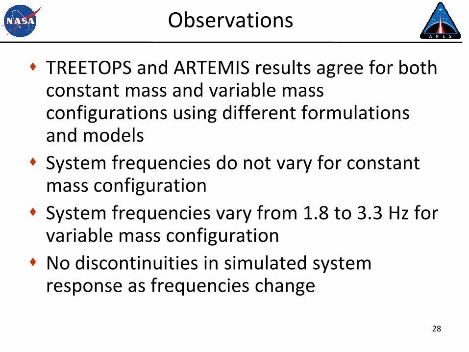
Observations

TREETOPS and ARTEMIS results agree for both constant mass and variable mass configurations using different formulations and models

System frequencies do not vary for constant mass configuration

System frequencies vary from 1.8 to 3.3 Hz for variable mass configuration

No discontinuities in simulated system response as frequencies change

29

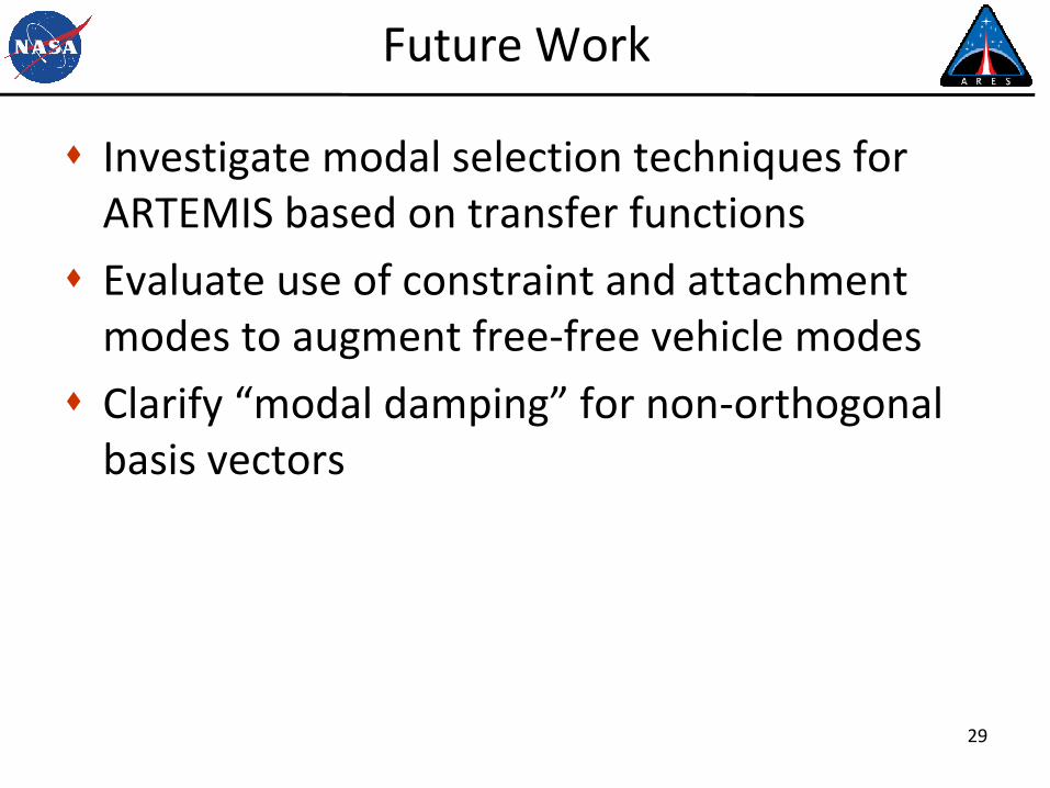
Future Work

Investigate modal selection techniques for ARTEMIS based on transfer functions

Evaluate use of constraint and attachment modes to augment free-free vehicle modes

Clarify “modal damping” for non-orthogonal basis vectors

30

References

Tobbe, P. A., “An Application of Component Modes to the Flexible Multibody Simulation Problem,” Ph.D. Dissertation, Dept. of Mechanical and Aerospace Engineering, Univ. of Alabama in Huntsville, Huntsville, AL, 1995.

Wilson, H. E., “Dynamics of Variable Mass Flexible Bodies with Time Varying Mode Shapes.” M.S. Thesis, Dept. of Mechanical and Aerospace Engineering, Univ. of Alabama in Huntsville, Huntsville, AL, 2007.

User’s Manual for TREETOPS, Rev. 8, Dynacs Inc, Clearwater, FL, 1990.

Craig, R. R., Structural Dynamics: An Introduction to Computer Methods, John Wiley & Sons, New York, 1981.

Goto, K., van de Geijn, R. A., “Anatomy of High-Performance Matrix Multiplication,” ACM Transactions on Mathematical Software, Vol. 34, No. 3, 2008, Article 12.

modeling and simulation of variable mass, flexible …...modeling and simulation of variable mass,...

Documents