modeling and simulation of pv array in matlab/simulink … of a buck converter. a pv array is...

International Research Journal of Engineering and Technology (IRJET) e-ISSN: 2395-0056

Volume: 04 Issue: 07 | July -2017 www.irjet.net p-ISSN: 2395-0072

© 2017, IRJET | Impact Factor value: 5.181 | ISO 9001:2008 Certified Journal | Page 2479

Modeling and Simulation of PV array in Matlab/Simulink for comparison of perturb and observe & incremental conductance

algorithms using buck converter

Sandeep Neupane1, Ajay Kumar2

1 M.Tech Scholar (Power electronics and drives), Swami Vivekanand Subharti University, Meerut, India 2 Asst. Prof., EEE Department, SITE, Swami Vivekanand Subharti University, Meerut, India

---------------------------------------------------------------------** *---------------------------------------------------------------------

Abstract - This paper defines modeling of solar PV array based on single diode PV cell equations in MATLAB/SIMULINK in order to compare MPPT tracking techniques using perturb and observe and incremental conductance algorithms making use of a buck converter. A PV array is modeled based on the electrical characteristics of PV module LG300N1C-G3. MPPT tracking techniques based on perturb and observe and incremental conductance algorithms are modeled in Simulink. A buck converter topology is used in Simulink for the comparison of maximum power point tracking. The simulation results show that tracking method using incremental conductance algorithm is better than that of perturb and observe algorithm.

Keywords: Photovoltaic, PV module, PV array, MPPT, P&O, INC, buck converter, MATLAB, SIMULINK.

1. INTRODUCTION Photovoltaic cell is a device based on a semiconductor material that converts energy of sunlight into electrical energy. Due to its low power, it is necessary to combine multiple cells into series or into parallel, forming a photovoltaic module and modules are further connected in series or into parallel with the required values of current and voltage to form a photovoltaic array. Output parameters of cells are most affected by environmental conditions, especially by solar irradiation and also by temperature at the input modules. Therefore, modeling this device necessarily requires ambient temperature and solar radiation as input variables. The output of the model can be voltage, current or power of the module. Any changes in the input variables are reflected by changes on the output. The common approach is to utilize the electrical equivalent circuit, which is primarily based on a light generated current source connected in parallel to a p-n junction diode. Many models have been proposed for the simulation of a solar cell or for a complete photovoltaic (PV) system at various solar intensities and temperature conditions [1-4]. The power conversion efficiency of solar module is very low. To increase efficiency of solar module proper impedance

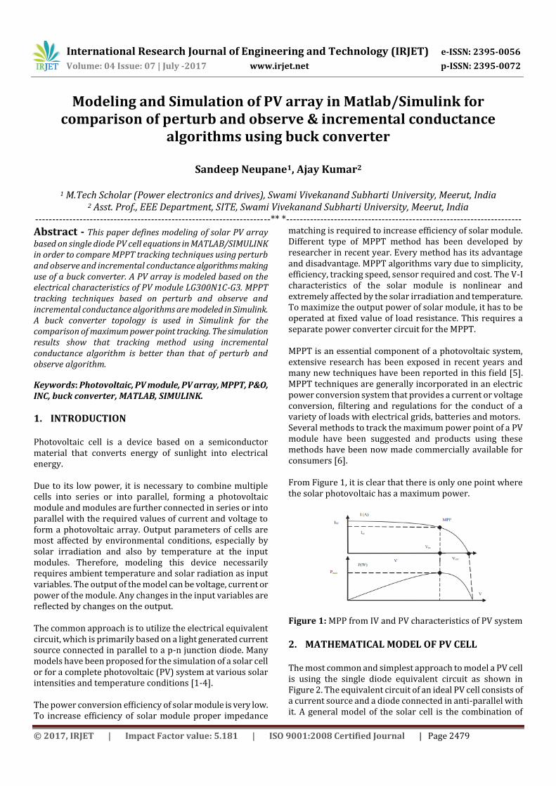
matching is required to increase efficiency of solar module. Different type of MPPT method has been developed by researcher in recent year. Every method has its advantage and disadvantage. MPPT algorithms vary due to simplicity, efficiency, tracking speed, sensor required and cost. The V-I characteristics of the solar module is nonlinear and extremely affected by the solar irradiation and temperature. To maximize the output power of solar module, it has to be operated at fixed value of load resistance. This requires a separate power converter circuit for the MPPT. MPPT is an essential component of a photovoltaic system, extensive research has been exposed in recent years and many new techniques have been reported in this field [5]. MPPT techniques are generally incorporated in an electric power conversion system that provides a current or voltage conversion, filtering and regulations for the conduct of a variety of loads with electrical grids, batteries and motors. Several methods to track the maximum power point of a PV module have been suggested and products using these methods have been now made commercially available for consumers [6]. From Figure 1, it is clear that there is only one point where the solar photovoltaic has a maximum power.

Figure 1: MPP from IV and PV characteristics of PV system

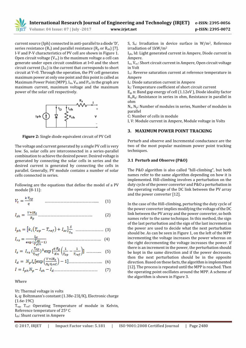
2. MATHEMATICAL MODEL OF PV CELL The most common and simplest approach to model a PV cell is using the single diode equivalent circuit as shown in Figure 2. The equivalent circuit of an ideal PV cell consists of a current source and a diode connected in anti-parallel with it. A general model of the solar cell is the combination of



© 2017, IRJET | Impact Factor value: 5.181 | ISO 9001:2008 Certified Journal | 480

current source (Iph) connected in anti-parallel to a diode ‘D’, series resistance (Rs) and parallel resistance (Rp or Rsh) [7]. I-V and P-V characteristics of PV cell are shown in Figure 1. Open circuit voltage (Voc) is the maximum voltage a cell can generate under open circuit condition at I=0 and the short circuit current (ISC) is the current that corresponds to short circuit at V=0. Through the operation, the PV cell generates maximum power at only one point and this point is called as Maximum Power Point (MPP). Im, Vm and Pm in the graph are maximum current, maximum voltage and the maximum power of the solar cell respectively.

Figure 2: Single diode equivalent circuit of PV Cell

The voltage and current generated by a single PV cell is very low. So, solar cells are interconnected in a series-parallel combination to achieve the desired power. Desired voltage is generated by connecting the solar cells in series and the desired current is generated by connecting the cells in parallel. Generally, PV module contains a number of solar cells connected in series. Following are the equations that define the model of a PV module [8-11]:

…………………………………………..... (1)

…………………………………………….. (2)

……………………… (3)

…………………………………. (4)

…………... (5)

…………………………... (6)

…………………………………… (7)

Where Vt: Thermal voltage in volts k, q: Boltzmann’s constant (1.38e-23J/K), Electronic charge (1.6e-19C) Top, Tref: Operating Temperature of module in Kelvin, Reference temperature of 250 C Ish: Shunt current in Ampere

S, Sn: Irradiation in device surface in W/m2, Reference irradiation of 1kW/m2 Iph, Id: Light generated current in Ampere, Diode current in Ampere. Isc, Voc: Short circuit current in Ampere, Open circuit voltage in Volt Irs: Reverse saturation current at reference temperature in Ampere Is: Diode saturation current in Ampere ki: Temperature coefficient of short circuit current Eg, n: Band gap energy of cell (1.12eV ), Diode ideality factor Rs,Rp: Resistance in series in ohm, Resistance in parallel in ohm Ns, Np: Number of modules in series, Number of modules in parallel C: Number of cells in module I, V: Module current in Ampere, Module voltage in Volts

3. MAXIMUM POWER POINT TRACKING Perturb and observe and Incremental conductance are the two of the most popular maximum power point tracking techniques. 3.1 Perturb and Observe (P&O) The P&O algorithm is also called “hill-climbing”, but both names refer to the same algorithm depending on how it is implemented. Hill-climbing involves a perturbation on the duty cycle of the power converter and P&O a perturbation in the operating voltage of the DC link between the PV array and the power converter [12]. In the case of the Hill-climbing, perturbing the duty cycle of the power converter implies modifying the voltage of the DC link between the PV array and the power converter, so both names refer to the same technique. In this method, the sign of the last perturbation and the sign of the last increment in the power are used to decide what the next perturbation should be. As can be seen in Figure 1, on the left of the MPP incrementing the voltage increases the power whereas on the right decrementing the voltage increases the power. If there is an increment in the power, the perturbation should be kept in the same direction and if the power decreases, then the next perturbation should be in the opposite direction. Based on these facts, the algorithm is implemented [12]. The process is repeated until the MPP is reached. Then the operating point oscillates around the MPP. A scheme of the algorithm is shown in Figure 3.




Figure 3: P&O Algorithm

3.2 Incremental Conductance (INC) The incremental conductance algorithm is based on the fact that the slope of the curve power vs. voltage (current) of the PV module is zero at the MPP, positive (negative) on the left of it and negative (positive) on the right, as can be seen in Figure 1 ΔV/ΔP = 0 (ΔI/ΔP = 0 ) at the MPP ΔV/ΔP > 0 (ΔI/ΔP < 0) on the left of MPP ΔV/ΔP < 0 (ΔI/ΔP > 0) on the right of MPP By comparing the increment of the power versus the increment of the voltage (current) between two consecutives samples, the change in the MPP voltage can be determined. A scheme of the algorithm is shown in Figure 4. Similar schemes can be found in [12-13].Here also, operating points oscillates around MPP.

Figure 4: INC Algorithm

4. BUCK CONVERTER A buck converter, or a standard step down converter, is a DC/DC converter used to decrease DC voltage. A schematic of a buck converter can be seen in Figure 5 and consists of one switch, one diode, one capacitor and one inductor.

Figure 5: Buck converter

The buck converter either store energy in the inductor or discharge the stored energy to the load, which is done in two different phases. To store energy, the switch connects the input voltage to the inductor which results in a positive voltage over the inductor, this phase is called on-time, ton. When the switch is disconnected, the positive side of the inductor is connected to the ground via a diode which results in a negative voltage over the inductor. The energy is then discharged from the inductor to the load, referred to as off-time, tof f , seen in Figure 6 [14].

Figure 6: Inductor current and voltage of a Standard Buck Converter

5. MODELING OF SYSTEM IN SIMULINK Figure 7 shows the block diagram of the system under consideration.

Figure 7: Block diagram of system




5.1 Modeling of PV array The mathematical equations given in section II (equation 1 to equation 6) have been written in Simulink using tags, constant and Math block. Since a single module has Ns=Np=1, this value of Np has been used. The generated current is thus the difference between Iph and (Id + Ish). Hence, Id is subtracted from Iph using subtract block and the output is fed to controlled current source. The rest of the model has been drawn as shown in Figure 2 to get Simulink model of equation 7. In order to model a PV module, circuit based approach has been used. Several PV modules are connected in series or parallel to get the PV array having desired output voltage and current. The development of PV array using mathematical equations and circuit based approach of PV cell is shown in Figure 8. Now, the PV array blocks modeled by using PV modules in series or in parallel are grouped into subsystem to form a PV array in Simulink that accepts irradiation in W/m2 and temperature in degree centigrade and provides array current and voltage that can be measured using current measurement and voltage measurement block respectively. The 300 W LG300N1C-G3 solar module is taken as the reference module for modelling and simulation .The parameters of the module is given in Table1. The value of series resistance is small, usually in the range of (0-1) Ω while that of parallel resistance is large, usually in the range of (100-1000) Ω. Similarly, ideality factor is in the range of (2/3-2). In this paper, the value of Rp, Rs and n are chosen as 212.8143, 0.31448 and 0.96984 respectively.

Figure 8: Modeling of PV array in Simulink

Table 1: Module Data of LG300N1C-G3 solar module

Module Data STC parameters (250C,1kW/m2)

Maximum Power 300 W

MPP voltage 32 V

MPP current 9.42 A

Open circuit voltage 39.5 V

Short circuit current 10 A

Number of cells 60

ki 0.03

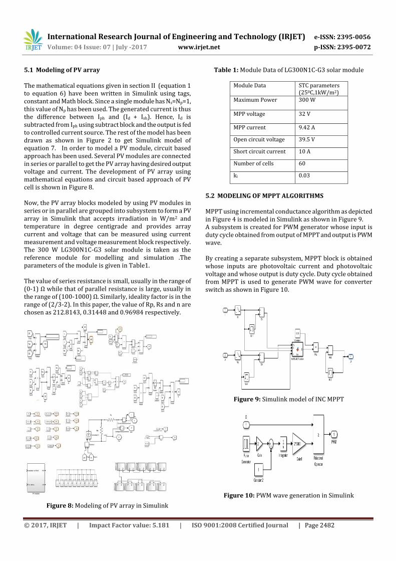
5.2 MODELING OF MPPT ALGORITHMS MPPT using incremental conductance algorithm as depicted in Figure 4 is modeled in Simulink as shown in Figure 9. A subsystem is created for PWM generator whose input is duty cycle obtained from output of MPPT and output is PWM wave. By creating a separate subsystem, MPPT block is obtained whose inputs are photovoltaic current and photovoltaic voltage and whose output is duty cycle. Duty cycle obtained from MPPT is used to generate PWM wave for converter switch as shown in Figure 10.

Figure 9: Simulink model of INC MPPT

Figure 10: PWM wave generation in Simulink




Similarly, MPPT using perturb and observe algorithm as depicted in Figure 3 is modeled in simulink which is shown in Figure 11.

Figure 11: Simulink model of P&O MPPT

In both simulink models, memory element is used to hold and hence compare the previous inputs with the present input for the functioning of the algorithm. Matlab function is employed where matlab codes are written for the implementation of the algorithm. 5.3 MODELING OF BUCK CONVERTER Buck converter circuit diagram as depicted in Figure 5 is drawn in Simulink to model DC-DC converter. This circuit is used as a subsystem to create a buck converter block that connects positive and negative terminal of PV array and PWM wave generated by PWM wave generator on input side and positive and negative terminal of load on the output side.

Figure 12: Simulink model of buck converter

5.4 MODELING OF THE SYSTEM The above modeled subsystems in Simulink are now connected to obtain the Simulink model of the system under consideration. Ten PV modules connected in parallel are used as a PV array model. MPPT with P&O or INC algorithm is used in MPPT &PWM block and buck converter is used as a dc to dc converter. Figure 13 shows the Simulink model of the overall system under consideration.

Figure 13: Simulink model of the system under consideration

A capacitance of 0.025F is used between PV array and buck converter and the parameters for buck converter used is L=10e-6H and C=1000e-6 F. A diode and a lead acid battery of 24 V, 1000 Ah is used as a load of buck converter. Since the library components used in the model are of Simscape, it requires powergui block available in library to run the simulation. Hence, powergui block has been added and used in continuous mode and ideal switching device. Signal generator block is used to provide variable input. The temperature input block is set to 250 C using constant block while variable input is used for irradiation input.

6. RESULTS AND DISCUSSIONS The P-V and I-V curves of the photovoltaic array model were first tested at STC and the result obtained was as shown in Figure 14. It can be seen from Figure 14 that the peak power of the array is 3000 W, open circuit voltage is 39.5 V and short circuit current is 100 A. If we compare this data with that of a module as given in Table 1, we see that the peak power and short circuit current has increased by a factor of 10 but open




Figure 14: I-V and P-V curve of PV array at STC

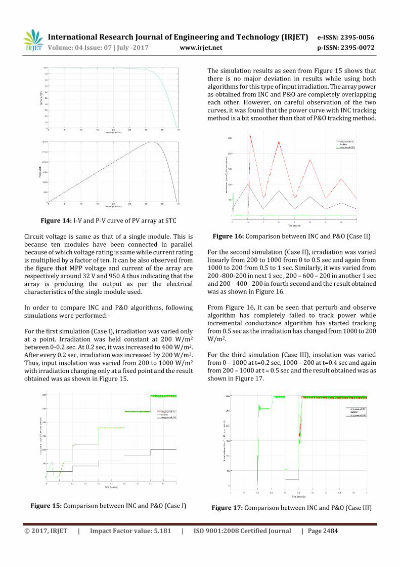
Circuit voltage is same as that of a single module. This is because ten modules have been connected in parallel because of which voltage rating is same while current rating is multiplied by a factor of ten. It can be also observed from the figure that MPP voltage and current of the array are respectively around 32 V and 950 A thus indicating that the array is producing the output as per the electrical characteristics of the single module used. In order to compare INC and P&O algorithms, following simulations were performed:- For the first simulation (Case I), irradiation was varied only at a point. Irradiation was held constant at 200 W/m2 between 0-0.2 sec. At 0.2 sec, it was increased to 400 W/m2. After every 0.2 sec, irradiation was increased by 200 W/m2. Thus, input insolation was varied from 200 to 1000 W/m2 with irradiation changing only at a fixed point and the result obtained was as shown in Figure 15.

Figure 15: Comparison between INC and P&O (Case I)

The simulation results as seen from Figure 15 shows that there is no major deviation in results while using both algorithms for this type of input irradiation. The array power as obtained from INC and P&O are completely overlapping each other. However, on careful observation of the two curves, it was found that the power curve with INC tracking method is a bit smoother than that of P&O tracking method.

Figure 16: Comparison between INC and P&O (Case II)

For the second simulation (Case II), irradiation was varied linearly from 200 to 1000 from 0 to 0.5 sec and again from 1000 to 200 from 0.5 to 1 sec. Similarly, it was varied from 200 -800-200 in next 1 sec , 200 – 600 – 200 in another 1 sec and 200 – 400 –200 in fourth second and the result obtained was as shown in Figure 16. From Figure 16, it can be seen that perturb and observe algorithm has completely failed to track power while incremental conductance algorithm has started tracking from 0.5 sec as the irradiation has changed from 1000 to 200 W/m2. For the third simulation (Case III), insolation was varied from 0 – 1000 at t=0.2 sec, 1000 – 200 at t=0.4 sec and again from 200 – 1000 at t = 0.5 sec and the result obtained was as shown in Figure 17.

Figure 17: Comparison between INC and P&O (Case III)




It can be seen from Figure 17 that both incremental conductance algorithm and perturb and observe algorithm has started tracking at 0.2 sec. However, when the input is constant after 0.5 sec, incremental conductance algorithm has reached steady state value earlier than perturb and observe algorithm. For the fourth simulation (Case IV) , the irradiation was varied rapidly between 200 - 1000 -200 in the first one second, 200 – 1000 from t= 1 to t=2 seconds, 1000 – 600 from t=2 to t=2.5 seconds and from 600 – 1000 from t= 2.5 to t= 4 seconds and fixed at 1000 from t= 4 to t=5 seconds. The result obtained was as shown in Figure 18.

Figure 18: Comparison between INC and P&O (Case IV)

It can be clearly seen from Figure 18 that incremental conductance algorithm has started tracking at t= 0.5 second where input irradiation has been varied between 1000 to 200 W/m2. On the other hand, perturb and observe algorithm has started tracking just after three seconds where input irradiation has been varied between 600 to 1000 W/m2. The output power from both algorithms is same after three seconds. From each of the cases discussed above, the incremental conductance tracking method has proved either equal or better than the perturb and observe tracking method.

7. CONCLUSION This paper has presented a photovoltaic array modeled using Matlab/Simulink to compare MPPT tracking techniques using P&O and INC algorithms. PV module has been modeled by using its equivalent circuit and the equations involved, for the system simulation. Using datasheet of LG300N1C-G3 solar module, the PV module has been developed and by connecting modules in parallel, PV array has been developed and simulated using Simulink of Matlab R2016b software package. MPPT tracking techniques has been modeled using P&O and INC algorithms and buck converter topology has been used. The simulation results has shown that incremental conductance algorithm

provides faster, better dynamic response and more reliable tracking method compared to perturb and observe algorithm when both are subjected to rapidly changing irradiation level.

REFERENCES [1] J.A.Gow; C.D Manning; "Development of a photovoltaic

array model for use in power-electronics simulation studies," Electric Power Applications, IEE Proceedings - , vol.146, no.2, pp.193-200, Mar 1999.

[2] S.Etienne; T. Alberto and S. Mikhaïl; “Explicit model of photovoltaic panels to determine voltages and currents at the maximum power point”. Sol Energy 2011;85(5), pp. 713-22.

[3] T.H.Liang. “Insolation-oriented model of photovoltaic module using Matlab/simulink”. Sol Energy 2010;84(7), pp.1318-26.

[4] I.Kashif; S. Zainal and T. Hamed. “Simple, fast and accurate two diode model for photovoltaic modules”. Sol Energy Mater Sol Cells 2011;95(2), pp. 586-94.

[5] Y.H.Chang and C.Y. Chang, "A Maximum Power Point Tracking of PV System by Scaling Fuzzy Control," presented at International Multi Conference of Engineers and Computer Scientists, HongKong, 2010.

[6] S.Mekhilef, "Performance of grid connected inverter with maximum power point tracker and power factor control," International Journal of Power Electronics, vol.1, pp. 49-62.

[7] M. G. Villalva, J. R. Gazoli, and E. R. Filho, “Comprehensive approach to modeling and simulation of photovoltaic arrays,”IEEE Trans. on power Electron. vol.24, no.5, pp.1198-1208, May 2009.

[8] S. S. Mohammed, “Modeling and simulation of photovoltaic module using matlab/simulink” International Journal of Chemical and Environmental Engineering, vol. 2, no. 5, pp. 350–355, 2011.

[9] S. Gomathy, S. Saravanan, and D. S. Thangavel, “Design and implementation of maximum power point tracking algorithm for a standalone pv system,” International journal of scientific and engineering research, vol. 3, no. 3, 2012.

[10] A. Grama, M. Dan and E. Lázár, "Photovoltaic panel model using Matlab," 2016 39th International Spring Seminar on Electronics Technology (ISSE), Pilsen, 2016, pp. 322-327.




[11] P. Suskis and I. Galkin, "Enhanced photovoltaic panel model for MATLAB-simulink environment considering solar cell junction capacitance," IECON 2013 - 39th Annual Conference of the IEEE Industrial Electronics Society, Vienna, 2013, pp. 1613-1618.

[12] T. Esram, P.L. Chapman, "Comparison of Photovoltaic Array Maximum Power Point Tracking Techniques," IEEE Transactions on Energy Conversion, vol. 22, no. 2, pp. 439449, June 2007.

[13] S. Jain, V. Agarwal, "Comparison of the performance of maximum power point tracking schemes applied to single-stage grid-connected photovoltaic systems," Electric Power Applications, IET, vol. 1, no. 5, pp. 753-762, Sept. 2007.

[14] N. Mohan, T. M. Undeland, W. P. Robbins, “Power Electronics: Converters, Applications, and Design”, 2nd ed., John Wiley & Sons, New York, 1995.

modeling and simulation of pv array in matlab/simulink … of a buck converter. a pv array is...

Documents