modeling and simulation of arsenate fate and … · epanet-msx (shang et al., 2008a, 2008b) was...

Water Distribution System Analysis 2010 – WDSA2010, Tucson, AZ, USA, Sept. 12-15, 2010

MODELING AND SIMULATION OF ARSENATE FATE AND TRANSPORT IN A DISTRIBUTION SYSTEM SIMULATOR

Stephen Klosterman1, Regan Murray2, Jeff Szabo2, John Hall2, and James Uber3

1Oak Ridge Institute for Science and Education, Oak Ridge, TN USA

2US Environmental Protection Agency, National Homeland Security Research Center, Cincinnati, OH USA

[email protected]

3University of Cincinnati, Cincinnati, OH USA

Abstract

Multi-species water quality models can be used to predict the fate and transport of contaminants such as arsenic in water distribution networks. In recent work, water quality models have been used to simulate hypothetical contamination events, estimate potential human health effects, and characterize the ability of sensors to detect contamination. Little work has been done to calibrate water quality models and validate them against experimental data generated in Distribution System Simulators (DSSs). In this paper, results are reported from bench scale and pilot scale experiments performed with a DSS at U. S. EPA’s Test and Evaluation Facility in Cincinnati, Ohio. The parameters for a reversible adsorption model were estimated from bench scale data generated over two days. The model was used with the EPANET-MSX software package to simulate the pilot scale experiment in the DSS. Model results match the pilot scale data very well for the first two days after the arsenate injection, however pilot scale data after this time deviates from model predictions. This deviation may be due to limitations in the time scale or sample size of the bench scale experiment. Additional modeling, simulation, and experimental work is planned to develop a fate and transport model that can be used in practical settings to design decontamination strategies following intentional arsenic contamination of water distribution systems. Keywords Water quality, modeling, simulation, adsorption, arsenic, arsenate, pipe wall reactions, parameter estimation, pilot scale experiments, bench scale experiments 1. BACKGROUND AND MOTIVATION In the last several years, several water security research studies have been conducted to evaluate the potential for contaminant adsorption to pipe walls, and to identify possible decontamination methods (Welter et al., 2008; U. S. EPA, 2008; Morrow et al., 2008). These studies considered a wide range of contaminants including metals, organic chemicals, bacteria, viruses, and toxins, exposed to several different pipe materials such as iron, copper, and PVC. Bench scale experiments were conducted to measure adsorption under various conditions; water quality parameters including pH, temperature, hardness, and TOC, and pipe wall conditions including pipe age, biofilm age, and type of pipe lining were varied in these experiments. Pilot scale pipe loop studies measured adsorption potential under more realistic conditions involving larger areas of exposed pipe subjected to different flow and mixing conditions. Together, these studies


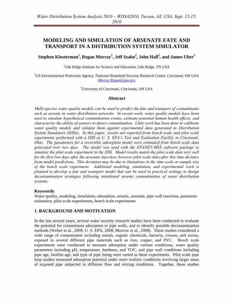
indicate the conditions under which contaminant adsorption may be likely, and identify several strategies for removing contaminants from pipe walls. Predictive models, however, are needed in order to quantify the risk to human health from contaminant adsorption and to design effective decontamination strategies. Water quality characteristics in real water distribution networks vary on daily, seasonal, and longer time scales; predictive models can be used to extrapolate results to a broader range of conditions. In addition, predictive models can account for system-scale behavior, such as mixing of multiple source waters, change in flow directions due to customer demands, and customer exposure to contaminants. Finally, predictive models can be used to determine the area in need of decontamination, the optimal locations for introducing decontamination agents, and the desired flushing times and velocities. The purpose of this paper is to validate a predictive model for arsenic adsorption to iron pipe using data from experiments performed at the EPA’s Test and Evaluation (T&E) Facility. A pilot-scale distribution system simulator (DSS) was constructed several years ago to support decontamination studies (U. S. EPA, 2008). Additional experiments were conducted as part of this study to provide the data needed for predictive models. The new experiments provided a denser set of time measurements in order to investigate the kinetics of adsorption. Arsenic was selected for this study because it is a known public health risk at low concentrations and it has an affinity for the iron oxide surfaces prevalent in corroded iron pipes (Lytle et al., 2004). The ultimate goal of this work is to describe the fate and transport of arsenic in drinking water pipes. This study focuses on arsenate adsorption to pipe walls. Future work will consider arsenite, which may undergo oxidation to arsenate in addition to adsorption and desorption. This paper is organized as follows. The physical components and operation of the DSS, as well as the experimental design of the arsenic experiment, are described in Section 2. The modeling and simulation methodology are described in Section 3, including the network model of the DSS, the reaction model for arsenic adsorption, and the bench scale experiments and parameter estimation. In Section 4, the experimental results are compared to model predictions and in Section 5, results are discussed and future work is outlined. The EPANET and EPANET-MSX input files are provided in Appendices A and B. 2. DISTRIBUTION SYSTEM SIMULATOR AND PILOT SCALE EXPERIMENTAL DESIGN The Distribution System Simulator (DSS) was constructed in 2005 to support several water quality and water security research projects. It has since been modified to support varied experimental designs. The current design and operation is described here. 2.1 The Distribution System Simulator The DSS, depicted in Figure 1, is constructed primarily from polyvinyl chloride (PVC) pipe. The components of the DSS include the large main tank that supplies tap water to the pipe loop, approximately 23 m of PVC pipe, mostly 15 cm diameter with some 5 and 10 cm diameter pipes, a 379 L stainless steel recirculation tank in-line with the main pipe, several pumps, and the associated valves and electronic control devices necessary to operate the system. While there are


three pumps in the DSS, only one pump was used for this experiment. The total volume of the DSS, including the recirculation tank, is approximately 833 L, and the DSS surface area in contact with the water is approximately 16 m2. The recirculation tank was observed to be completely mixed during a dye tracer test. Before the recirculation tank, a series of small circular coupons 2.54 cm in diameter, made from used cast iron, were threaded and screwed into a section of the DSS such that the wetted surfaces were flush with the interior pipe surface. The 30 coupons were fabricated from an iron pipe taken out of service from the Greater Cincinnati Water Works (GCWW) distribution system. The total pipe wall surface area of the coupons in contact with the water was 152 cm2. Coupons were removed by stopping flow in the loop, isolating the pipe section holding the coupons, and unscrewing the coupon. PVC plugs replaced the coupons before flow was resumed.

Figure 1. Distribution System Simulator (DSS) at the T&E facility.

Inset. The coupon removal process. The DSS is equipped with sensors that continuously measure basic water quality parameters such as pH, turbidity, free chlorine, total chlorine, specific conductivity, temperature, and oxidation-reduction potential. In addition, continuous measurements of pressure and flow are taken. All sensors were calibrated before data collection began and maintained according to the manufacturers’ recommendations throughout the experiment. 2.2 Operation of the DSS During the arsenic experiment, a pump was used to maintain a flow of 315 ± 1 L/min in the DSS, which is in the turbulent regime. Previous experiments operated the DSS in recirculation mode, essentially creating a large batch reactor. In this experiment, however, water was allowed to leave the system from an overflow in the recirculation tank, and a constant input of new tap water entered the system from the main tank at a rate of 3 L/min. Continuous introduction of tap water

Pipe Loop

Recirculation Tank

Main Tank

Control Panel

Removable Pipe Section


at this rate was found to maintain water quality parameters such as temperature and pH in the DSS at constant levels. When coupons were removed from the DSS for analysis, the pump was stopped to relieve system pressure. This also caused flow in the DSS as well as the input and output flows to stop. 2.3 Experimental Methodology Prior to the arsenic experiment, the coupons were conditioned in the DSS for a period of 54 days, allowing the coupon materials to corrode and biofilm to grow. The system pH and temperature were approximately 8.5 and 20 °C. A control coupon was taken one day before the contaminant injection for arsenic analysis and to confirm biofilm growth. The heterotrophic plate count (HPC) was measured by Standard Method 9215C (Clesceri et al., 1998). According to this method, the corrosion material was scraped into 10 mL of sterile monopotassium phosphate buffer (pH 7.2). The corrosion material was then broken up with a glass stirring rod and serially diluted and plated. The arsenic analysis method is described below. The control results are described in Section 4. The arsenic experiment began with a 31 second injection of one liter of sodium arsenate solution containing 1.2 g/L arsenic into the DSS using a pressurized syringe fabricated at the T&E Facility. The injection solution was prepared with 99% sodium arsenate heptahydrate (Sigma-Aldrich, St. Louis, MO). Samples of the bulk water and coupons were taken at prescribed times throughout the 7 day experiment. Duplicate coupon samples were removed at 3, 11, 23 and 41 minutes, and 1.2, 2.2, 3.3, 5.3, 7.3, 24, 48, and 72 hours after injection of arsenic; a triplicate sample was harvested at 143 hours. Bulk phase samples were collected at 4, 8, 10, 15, 22, and 45 minutes and 1.3, 2.3, 3.3, 4.3, 5.6, 6.4, 7.3, 24, 50, 72 and 144 hours after injection. Bulk phase samples were taken from a tap built into the DSS. The tap was opened at each sampling time and at least 10 mL was drained into a new 50 mL polypropylene sampling tube. After removal, the coupon surfaces were scraped with a clean, sterile scalpel and the corrosion/biofilm material was deposited into clean, pre-weighed porcelain 30 mL crucibles. To remove any residual material, the scraped coupon surface and scalpel were rinsed with deionized water, which was also collected in the crucible. The crucible was placed in a 60º C oven for 24 hours or until the rinse water evaporated. The crucible was allowed to cool and was reweighed to determine the mass of solids scraped from the coupon. The solids were then digested with nitric acid using Standard Methods 3030D and E (Clesceri et al., 1998). Once digested, the sample was analyzed for arsenic by Inductively Coupled Plasma – Optical Emission Spectroscopy (ICP-OES) using Standard Method 3120B. Bulk phase samples were analyzed using the same method with no digestion. 3. MODELING AND SIMULATION EPANET-MSX (Shang et al., 2008a, 2008b) was used to simulate the hydraulics and the water quality reactions in the DSS during the experiment. EPANET-MSX requires as input a network model describing the topology and operation of the DSS and a mathematical model for reactions


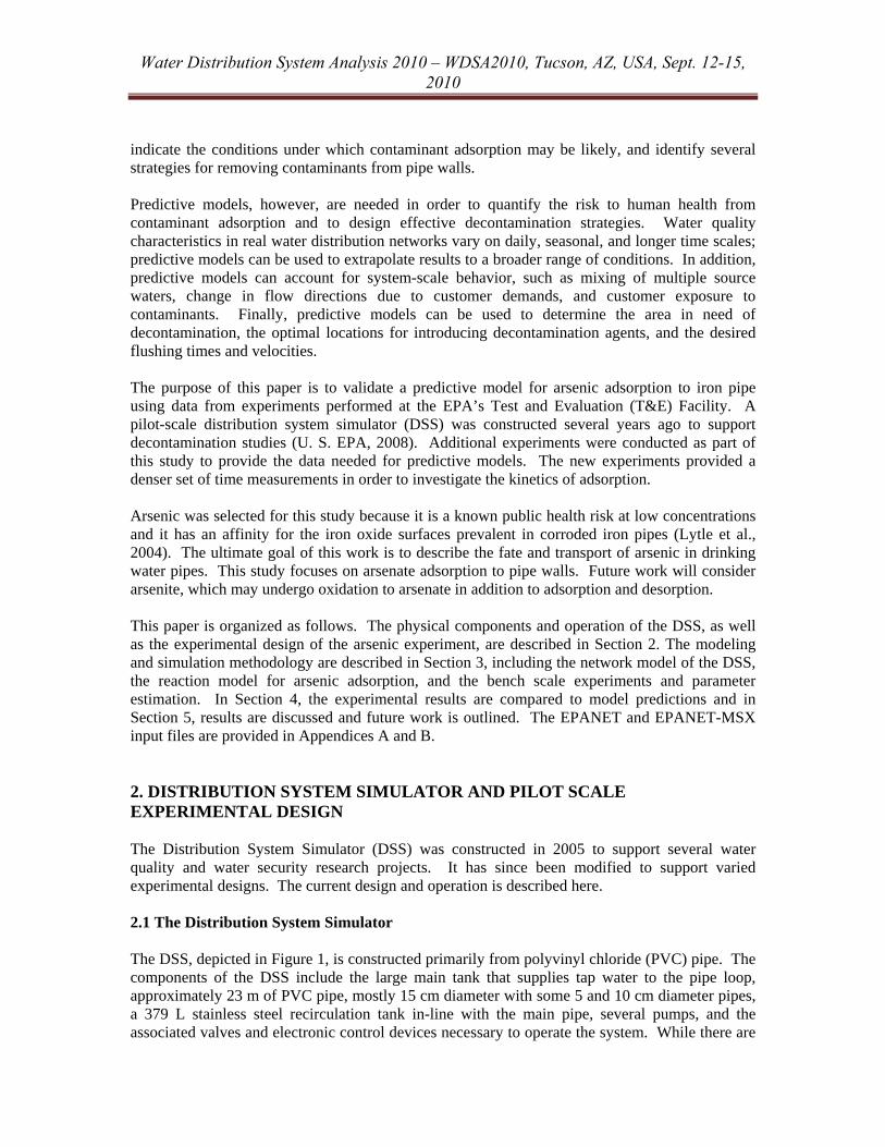
to be simulated in the pipe network. These are described below and the files provided in Appendices A and B. 3.1 Network model A network model of the DSS was created and is shown in Figure 2. The pipe lengths and diameters for the model were defined based on measurements taken by the authors. The modeled system does not include dead-end pipes and pipes which were valved off during the experiment; therefore, the total volume and surface area of the modeled DSS are 802 L and 14.5 m2, slightly lower than the estimates of the full DSS given above. The recirculation tank was modeled as completely mixed. A modeled pump was used to maintain the experimental flow rate of 315 L/min. The main tank was not included in the model, but was represented by a negative demand, or input, of 3 L/min assigned to the node before the pump, which is where the main tank connects to the DSS. An equivalent positive demand, or output, was assigned to the node after the recirculation tank, to model the gradual removal of water from the DSS. The modeled pump was turned off and both demands were set to zero during each coupon sampling event.

Figure 2. Diagram of the DSS network model as visualized in EPANET.

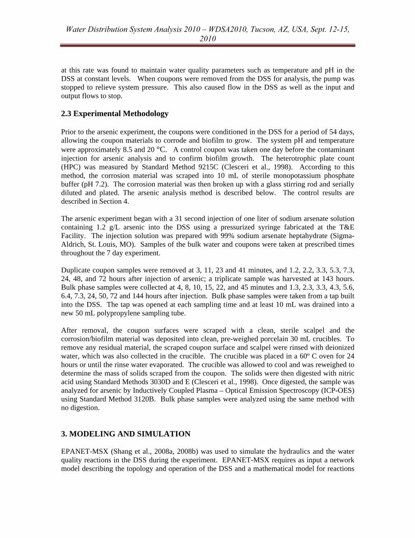
3.2 Reaction Model The mathematical model described by Equations (1) and (2) was used to predict the change with respect to time (t) of arsenic concentrations in the bulk water and adsorbed to the pipe walls (Koopal et al., 2001):

(1)

(2)

where C is the bulk concentration of arsenate (mg/L), P is the concentration of arsenate adsorbed to the coupons (mg/m2

pipe surface area), Smax is the maximum capacity of a coupon for adsorbed


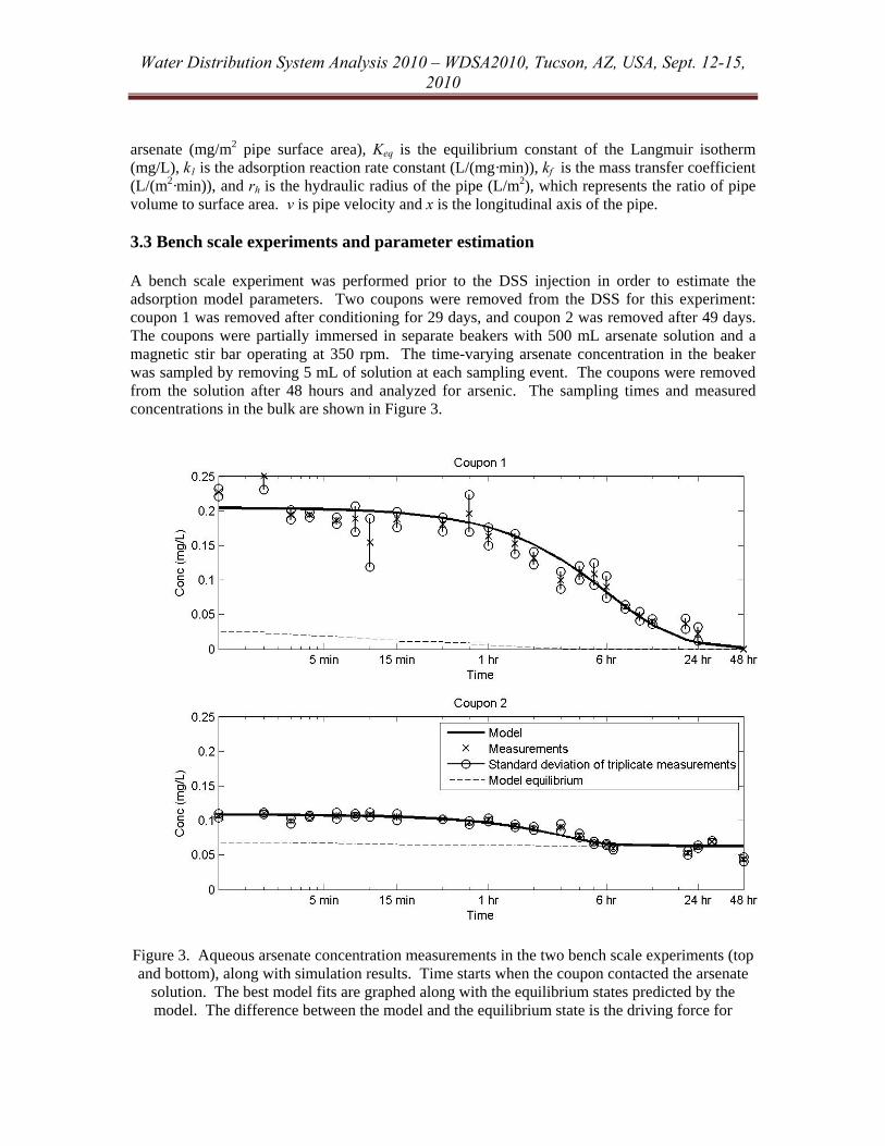
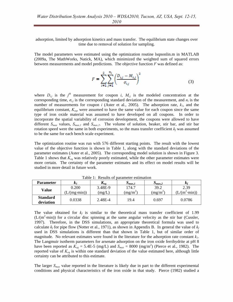
arsenate (mg/m2 pipe surface area), Keq is the equilibrium constant of the Langmuir isotherm (mg/L), k1 is the adsorption reaction rate constant (L/(mg·min)), kf is the mass transfer coefficient (L/(m2·min)), and rh is the hydraulic radius of the pipe (L/m2), which represents the ratio of pipe volume to surface area. v is pipe velocity and x is the longitudinal axis of the pipe. 3.3 Bench scale experiments and parameter estimation A bench scale experiment was performed prior to the DSS injection in order to estimate the adsorption model parameters. Two coupons were removed from the DSS for this experiment: coupon 1 was removed after conditioning for 29 days, and coupon 2 was removed after 49 days. The coupons were partially immersed in separate beakers with 500 mL arsenate solution and a magnetic stir bar operating at 350 rpm. The time-varying arsenate concentration in the beaker was sampled by removing 5 mL of solution at each sampling event. The coupons were removed from the solution after 48 hours and analyzed for arsenic. The sampling times and measured concentrations in the bulk are shown in Figure 3.

Figure 3. Aqueous arsenate concentration measurements in the two bench scale experiments (top and bottom), along with simulation results. Time starts when the coupon contacted the arsenate

solution. The best model fits are graphed along with the equilibrium states predicted by the model. The difference between the model and the equilibrium state is the driving force for


adsorption, limited by adsorption kinetics and mass transfer. The equilibrium state changes over

time due to removal of solution for sampling. The model parameters were estimated using the optimization routine lsqnonlin.m in MATLAB (2009a, The MathWorks, Natick, MA), which minimized the weighted sum of squared errors between measurements and model predictions. The objective function F was defined as:

(3)

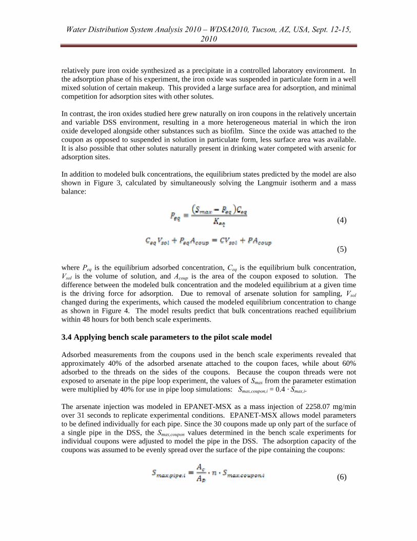
where Di,j is the jth measurement for coupon i, Mi,j is the modeled concentration at the corresponding time, σi,j is the corresponding standard deviation of the measurement, and ni is the number of measurements for coupon i (Aster et al., 2005). The adsorption rate, k1, and the equilibrium constant, Keq, were assumed to have the same value for each coupon since the same type of iron oxide material was assumed to have developed on all coupons. In order to incorporate the spatial variability of corrosion development, the coupons were allowed to have different Smax values, Smax,1 and Smax,2. The volume of solution, beaker, stir bar, and stir bar rotation speed were the same in both experiments, so the mass transfer coefficient kf was assumed to be the same for each bench scale experiment. The optimization routine was run with 576 different starting points. The result with the lowest value of the objective function is shown in Table 1, along with the standard deviations of the parameter estimates (Aster et al., 2005). The corresponding model solution is shown in Figure 3. Table 1 shows that Keq was relatively poorly estimated, while the other parameter estimates were more certain. The certainty of the parameter estimates and its effect on model results will be studied in more detail in future work.

Table 1: Results of parameter estimation Parameter k1 Keq Smax,1 Smax,2 kf

Value 0.200 (L/(mg·min))

3.48E-9 (mg/L)

174.7 (mg/m2)

39.2 (mg/m2)

2.39 (L/(m2·min))

Standard deviation 0.0338 2.48E-4 19.4 0.697 0.0786

The value obtained for kf is similar to the theoretical mass transfer coefficient of 1.99 (L/(m2·min)) for a circular disc spinning at the same angular velocity as the stir bar (Cussler, 1997). Therefore, in the DSS simulations, an appropriate theoretical formula was used to calculate kf for pipe flow (Notter et al., 1971), as shown in Appendix B. In general the value of kf used in DSS simulations is different than that shown in Table 1, but of similar order of magnitude. No relevant estimates were found in the literature for the adsorption rate constant k1. The Langmuir isotherm parameters for arsenate adsorption on the iron oxide ferrihydrite at pH 8 have been reported as Keq = 5.4E-5 (mg/L) and Smax = 8000 (mg/m2) (Pierce et al., 1982). The reported value of Keq is within one standard deviation of the value estimated here, although little certainty can be attributed to this estimate. The larger Smax value reported in the literature is likely due in part to the different experimental conditions and physical characteristics of the iron oxide in that study. Pierce (1982) studied a


relatively pure iron oxide synthesized as a precipitate in a controlled laboratory environment. In the adsorption phase of his experiment, the iron oxide was suspended in particulate form in a well mixed solution of certain makeup. This provided a large surface area for adsorption, and minimal competition for adsorption sites with other solutes. In contrast, the iron oxides studied here grew naturally on iron coupons in the relatively uncertain and variable DSS environment, resulting in a more heterogeneous material in which the iron oxide developed alongside other substances such as biofilm. Since the oxide was attached to the coupon as opposed to suspended in solution in particulate form, less surface area was available. It is also possible that other solutes naturally present in drinking water competed with arsenic for adsorption sites. In addition to modeled bulk concentrations, the equilibrium states predicted by the model are also shown in Figure 3, calculated by simultaneously solving the Langmuir isotherm and a mass balance:

(4)

(5) where Peq is the equilibrium adsorbed concentration, Ceq is the equilibrium bulk concentration, Vsol is the volume of solution, and Acoup is the area of the coupon exposed to solution. The difference between the modeled bulk concentration and the modeled equilibrium at a given time is the driving force for adsorption. Due to removal of arsenate solution for sampling, Vsol changed during the experiments, which caused the modeled equilibrium concentration to change as shown in Figure 4. The model results predict that bulk concentrations reached equilibrium within 48 hours for both bench scale experiments. 3.4 Applying bench scale parameters to the pilot scale model Adsorbed measurements from the coupons used in the bench scale experiments revealed that approximately 40% of the adsorbed arsenate attached to the coupon faces, while about 60% adsorbed to the threads on the sides of the coupons. Because the coupon threads were not exposed to arsenate in the pipe loop experiment, the values of Smax from the parameter estimation were multiplied by 40% for use in pipe loop simulations: Smax,coupon,i = 0.4 · Smax,i. The arsenate injection was modeled in EPANET-MSX as a mass injection of 2258.07 mg/min over 31 seconds to replicate experimental conditions. EPANET-MSX allows model parameters to be defined individually for each pipe. Since the 30 coupons made up only part of the surface of a single pipe in the DSS, the Smax,coupon values determined in the bench scale experiments for individual coupons were adjusted to model the pipe in the DSS. The adsorption capacity of the coupons was assumed to be evenly spread over the surface of the pipe containing the coupons:

(6)


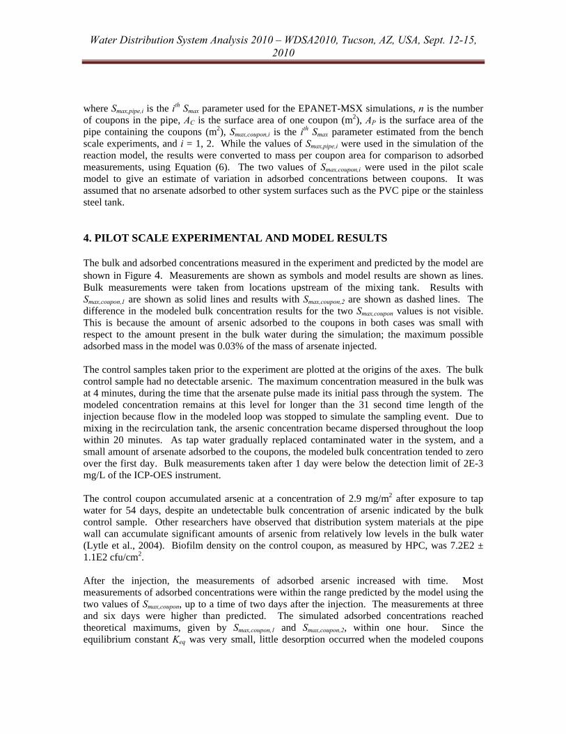
where Smax,pipe,i is the ith Smax parameter used for the EPANET-MSX simulations, n is the number of coupons in the pipe, AC is the surface area of one coupon (m2), AP is the surface area of the pipe containing the coupons (m2), Smax,coupon,i is the ith Smax parameter estimated from the bench scale experiments, and i = 1, 2. While the values of Smax,pipe,i were used in the simulation of the reaction model, the results were converted to mass per coupon area for comparison to adsorbed measurements, using Equation (6). The two values of Smax,coupon,i were used in the pilot scale model to give an estimate of variation in adsorbed concentrations between coupons. It was assumed that no arsenate adsorbed to other system surfaces such as the PVC pipe or the stainless steel tank. 4. PILOT SCALE EXPERIMENTAL AND MODEL RESULTS The bulk and adsorbed concentrations measured in the experiment and predicted by the model are shown in Figure 4. Measurements are shown as symbols and model results are shown as lines. Bulk measurements were taken from locations upstream of the mixing tank. Results with Smax,coupon,1 are shown as solid lines and results with Smax,coupon,2 are shown as dashed lines. The difference in the modeled bulk concentration results for the two Smax,coupon values is not visible. This is because the amount of arsenic adsorbed to the coupons in both cases was small with respect to the amount present in the bulk water during the simulation; the maximum possible adsorbed mass in the model was 0.03% of the mass of arsenate injected. The control samples taken prior to the experiment are plotted at the origins of the axes. The bulk control sample had no detectable arsenic. The maximum concentration measured in the bulk was at 4 minutes, during the time that the arsenate pulse made its initial pass through the system. The modeled concentration remains at this level for longer than the 31 second time length of the injection because flow in the modeled loop was stopped to simulate the sampling event. Due to mixing in the recirculation tank, the arsenic concentration became dispersed throughout the loop within 20 minutes. As tap water gradually replaced contaminated water in the system, and a small amount of arsenate adsorbed to the coupons, the modeled bulk concentration tended to zero over the first day. Bulk measurements taken after 1 day were below the detection limit of 2E-3 mg/L of the ICP-OES instrument. The control coupon accumulated arsenic at a concentration of 2.9 mg/m2 after exposure to tap water for 54 days, despite an undetectable bulk concentration of arsenic indicated by the bulk control sample. Other researchers have observed that distribution system materials at the pipe wall can accumulate significant amounts of arsenic from relatively low levels in the bulk water (Lytle et al., 2004). Biofilm density on the control coupon, as measured by HPC, was 7.2E2 ± 1.1E2 cfu/cm2. After the injection, the measurements of adsorbed arsenic increased with time. Most measurements of adsorbed concentrations were within the range predicted by the model using the two values of Smax,coupon, up to a time of two days after the injection. The measurements at three and six days were higher than predicted. The simulated adsorbed concentrations reached theoretical maximums, given by Smax,coupon,1 and Smax,coupon,2, within one hour. Since the equilibrium constant Keq was very small, little desorption occurred when the modeled coupons


came into contact with uncontaminated water; thus, desorption is not visible in the simulation results on Figure 4.

Figure 4. The control samples, taken shortly before the injection, are plotted at the origins of the axes. Bulk samples (top) were taken from the sample port, located after the coupons and before

the tank. The adsorbed concentrations (bottom) were from coupons removed during the experiment. Two model solutions based on parameters estimated from coupons removed before

the injection are shown. Of the triplicate coupons at 6 days, the two samples with higher concentrations appear identical.

5. DISCUSSION AND FUTURE WORK The top of Figure 4 shows that the model predictions of bulk concentration match the experimental measurements fairly well. The simulated bulk concentrations exhibit a similar temporal trend to the measurements, although most measurements are lower. This overestimation may have resulted because the model did not allow for transport of arsenic into dead-end and valved off pipes. These pipes were not included in the network model since they would have zero velocity; the advective transport algorithm of EPANET-MSX would not cause any mass to be transported into them. However a tracer study with a visible dye revealed that injected fluid does mix with the water in these pipe sections. This would have caused dilution of the bulk arsenic concentration in the main part of the loop, making it lower than the model predicted. Improvements to the hydraulic model may make it possible to model this behavior.


While the two coupons used for parameter estimation represent a small sample size, the range of simulated adsorbed concentrations based on these parameters match the experimental data remarkably well for the first two days, as seen on the bottom of Figure 4. This is the same time scale over which the data used to estimate parameters was collected. From two to six days, the measurements are significantly higher than the range of model predictions, which have already reached their theoretical maximum adsorption densities. While the coupons extracted later may have had higher adsorption capacities from the time of injection, the temporal trend in adsorbed measurements seems to suggest otherwise. The increase in measured adsorbed concentrations after two days is also interesting given there was no detectable arsenic in the bulk water. Low levels of arsenic may have persisted in the DSS due to reversible sorption to materials on surfaces of the PVC pipe or stainless steel tank. Assuming the bulk concentration in the DSS was at the detection limit from two to six days, sufficient arsenate would have been available to increase coupon concentrations by 450 mg/m2, more than enough to cause the observed increases. If this were the case, one possible explanation for the increase in adsorbed measurements after two days is that the coupons continued to corrode after the injection, increasing their adsorption capacities. This would allow for higher adsorbed concentrations than predicted above. The model could be adjusted to describe these phenomena by defining adsorption characteristics for the PVC pipes and stainless steel tank, and by allowing the Smax parameter to change with time. Of the two coupons used for parameter estimation, the one that was conditioned for a shorter time had a greater adsorption capacity. This is contrary to the intuitive hypothesis that a longer conditioning time would result in more corrosion and higher adsorption capacity. This suggests that variability between coupons is at least as important as the time of coupon conditioning for determining adsorption capacity, although the sample size of the bench scale experiment was limited. It is also not clear if the additional adsorption capacity observed in the pipe loop coupons from two to six days was developed after the arsenate injection, or if it was primarily due to the overall conditioning time of the coupons, including time spent in the loop before injection. Variability between coupons, and the relationship between conditioning time and adsorption capacity, should be investigated more thoroughly in future work. Bench scale experiments over longer time scales should be performed to investigate adsorption at later times, and other adsorption models may be explored. Additional modeling, simulation, and experimental work, including that described above, is being planned. This work will include a similar experiment involving the injection of arsenite. The model will be further developed to represent the oxidation of arsenite to arsenate. The resulting model will be applied to realistic network models in order to formulate effective decontamination strategies following intentional arsenic contamination of water distribution systems. ACKNOWLEDGEMENTS AND DISCLAIMER The U.S. Environmental Protection Agency through its Office of Research and Development funded and collaborated in the research described here under an Interagency Agreement with the Department of Energy’s ORISE fellowship program and Contract EP-C-09-041 with Shaw Environmental. It has been reviewed by the Agency and approved for publication but does not necessarily reflect the Agency’s views. No official endorsement should be inferred. EPA does


not endorse the purchase or sale of any commercial products or services. The authors would like to thank Greg Meiners, Tim Kling, Tim Gray, and Shekar Govindaswamy for their assistance with the experiments, and Terra Haxton and Dominic Boccelli for their helpful comments on the text.

References Aster, Richard C., Borchers, Brian, and Thurber, Clifford H. (2005) Parameter Estimation and Inverse Problems. Burlington, MA: Elsevier Academic Press. Clesceri, L. S., Greenberg, A. E., and Eaton, A. D. (1998) Standard Methods for the Examination of Water and Wastewater, 20th ed. Washington, DC: published jointly by the American Public Health Association, American Water Works Assocation, and the Water Environment Federation. Cussler, E. L. (1997) Diffusion: Mass Transfer in Fluid Systems. New York: Cambridge University Press. Koopal, Luuk K. and Avena, Marcelo J. (2001) "A simple model for adsorption kinetics at charged solid-liquid interfaces." Colloids and Surfaces A: Physicochemical and Engineering Aspects 192: 93-107. Lytle, Darren A., Sorg, Thomas J. and Frietch, Christy. (2004) "Accumulation of Arsenic in Drinking Water Distribution Systems." Environmental Science and Technology 38: 5365-5372. Notter, Robert H., and Sleicher, C. A. (1971) "The eddy diffusivity in the turbulent boundary layer near a wall." Chemical Engineering Science 26: 161-171. Pierce, Matthew L., and Moore, Carleton B. (1982) "Adsorption of arsenite and arsenate on amorphous iron hydroxide." Water Research 16: 1247-1253. Shang, Feng, Uber, James G. and Rossman, Lewis A. (2008a) "EPANET-MSX Software and Documentation" U.S. EPA - Homeland Security Research. August 8, 2008. http://www.epa.gov/nhsrc/water/teva.html#_epanet (accessed April 12, 2010). Shang, Feng, Uber, James G. and Rossman, Lewis A. (2008b) “Modeling Reaction and Transport of Multiple Species in Water Distribution Systems.” Environmental Science and Technology, 42: 808-814. Morrow, J. B., Almeida, J. L., Fitzgerald L. A. and K. D. Cole. (2008) “Association and decontamination of Bacillus spores in a simulated drinking water system.” Water Research 42: 5011-5021. U.S. Environmental Protection Agency. (2008) Pilot Scale Tests and Systems Evaluation for the Containment, Treatment, and Decontamination of Selected Materials from T&E Pipe Loop Equipment, EPA/600/R-08/016. Welter, G., Lechevallier, M., Cotruvo, J., Moser, R. and S. Spangler. (2008) Guidance for Decontamination of Water System Infrastructure. AWWA Research Foundation.


APPENDIX A: NETWORK MODEL FILE [TITLE] [JUNCTIONS] ;ID Elev Demand Pattern 3 0 3.028328 P1 ; 5 0 0 ; 6 0 0 ; 12 0 0 ; 13 0 0 ; 14 0 0 ; InjPort 0 0 ; 18 0 0 ; 2 0 0 ; 4 0 0 ; 7 0 0 ; 8 0 0 ; 9 0 -3.028328 P1 ; 10 0 0 ; 11 0 0 ; [TANKS] ;ID Elevation InitLevel MinLevel MaxLevel Diameter MinVol VolCurve 1 0 0.8382 0 0.8763 0.7493 0 [PIPES] ;ID Node1 Node2 Length Diameter Roughness MinorLoss Status 2 3 1 1.4986 51 100 0 Open ; 23 5 1 1.27 51 100 0 Open ;Rec Tk In Val 26 18 InjPort 1.1684 152.4 100 0 Open ;Std Flow In Val 6 12 5 2.2162 102 100 0 Open ; 7 3 6 1.2192 102 100 0 Open ; 8 14 2 0.4064 152.4 100 0 Open ; 13 4 13 0.4064 152.4 100 0 Open ; 1 InjPort 14 8.7884 152.4 100 0 Open ; 3 12 7 4.8768 152.4 100 0 Open ; 4 7 8 2.3622 152.4 100 0 Open ; 5 8 13 0.4826 152.4 100 0 Open ; 9 6 9 1.2954 51 100 0 Open ; 14 10 11 0.9906 51 100 0 Open ; 15 11 18 2.8448 102 100 0 Open ; 16 2 4 1.8288 152.4 100 0 Open ; [PUMPS] ;ID Node1 Node2 Parameters 11 9 10 HEAD 318LPM ; [PATTERNS] ;ID Multipliers ; Pattern for introduction of new water and removal of recirculation tank overflow water removed for space reasons [CURVES] ;ID X-Value Y-Value 318LPM 227 2 [CONTROLS] LINK 11 CLOSED AT TIME 0.022222 LINK 11 OPEN AT TIME 0.114722 LINK 11 CLOSED AT TIME 0.170833 LINK 11 OPEN AT TIME 0.220278 LINK 11 CLOSED AT TIME 0.375000 LINK 11 OPEN AT TIME 0.420833 LINK 11 CLOSED AT TIME 0.662500 LINK 11 OPEN AT TIME 0.728333 LINK 11 CLOSED AT TIME 1.208333 LINK 11 OPEN AT TIME 1.242778


LINK 11 CLOSED AT TIME 2.219444 LINK 11 OPEN AT TIME 2.255000 LINK 11 CLOSED AT TIME 3.245833 LINK 11 OPEN AT TIME 3.290278 LINK 11 CLOSED AT TIME 5.283333 LINK 11 OPEN AT TIME 5.327222 LINK 11 CLOSED AT TIME 7.250000 LINK 11 OPEN AT TIME 7.297778 LINK 11 CLOSED AT TIME 23.991667 LINK 11 OPEN AT TIME 24.059722 LINK 11 CLOSED AT TIME 48.000000 LINK 11 OPEN AT TIME 48.044722 LINK 11 CLOSED AT TIME 71.912500 LINK 11 OPEN AT TIME 71.971111 LINK 11 CLOSED AT TIME 143.333333 LINK 11 OPEN AT TIME 143.444444 [TIMES] Duration 168:00 Hydraulic Timestep 0:00:01 Quality Timestep 0:00:01 Pattern Timestep 0:00:01 Pattern Start 0:00 Report Timestep 1:00 Report Start 0:00 Start ClockTime 12 am Statistic NONE [REPORT] Status No Summary No Page 0 [OPTIONS] Units LPM Headloss H-W Specific Gravity 1 Viscosity 1 Trials 40 Accuracy 0.001 CHECKFREQ 2 MAXCHECK 10 DAMPLIMIT 0 Unbalanced Continue 10 Pattern 1 Demand Multiplier 1.0 Emitter Exponent 0.5 Quality None mg/L Diffusivity 1 Tolerance 0.01 [COORDINATES] ;Node X-Coord Y-Coord 3 1513.92 4454.76 5 2616.01 4454.76 6 1617.13 4772.73 12 2859.63 5011.60 13 7998.84 5011.60 14 8486.08 6322.51 InjPort 3312.06 6322.51 18 3010.44 5684.45 2 8648.49 6136.89 4 8230.86 5162.41 7 5760.49 5017.48 8 7508.74 5017.48 9 1756.99 5069.93 10 2263.99 5402.10 11 2631.12 5559.44


1 2082.37 4454.76 [LABELS] ;X-Coord Y-Coord Label & Anchor Node 3068.18 5489.51 "Sample Port" 6040.21 4930.07 "Coupons" 1407.34 6468.53 "Injection Port" 1092.66 4300.70 "Recirculating tank" [BACKDROP] DIMENSIONS 0.00 0.00 10000.00 10000.00 UNITS None FILE OFFSET 0.00 0.00 [END]


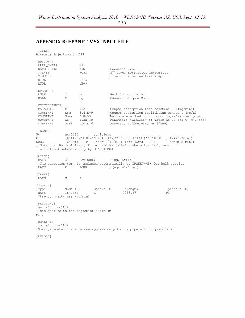
APPENDIX B: EPANET-MSX INPUT FILE [TITLE] Arsenate injection in DSS [OPTIONS] AREA_UNITS M2 RATE_UNITS MIN ;Reaction rate SOLVER ROS2 ;2nd order Rosenbrock integrator TIMESTEP 1 ;1 second solution time step RTOL 1E-5 ATOL 1E-5 [SPECIES] BULK C mg ;Bulk Concentration WALL P mg ;Adsorbed Coupon Conc [COEFFICIENTS] PARAMETER k1 0.2 ;Coupon adsorption rate constant (L/(mg*min)) CONSTANT Keq 3.48E-9 ;Coupon adsorption equilibrium constant (mg/L) CONSTANT Smax 0.8453 ;Maximum adsorbed coupon conc (mg/m^2) over pipe CONSTANT nu 8.3E-10 ;Kinematic viscosity of water at 20 deg C (m^2/sec) CONSTANT Diff 1.01E-6 ;Arsenate diffusivity (m^2/sec) [TERMS] Sc nu/Diff ;unitless kf (Diff/D)*0.0149*Re^(0.875)*Sc^(0.33333333)*60*1000 ;(L/(m^2*min)) SORB (C*(Smax - P) - Keq*C)/(1/k1 + 1/kf*(Smax - P)) ;(mg/(m^2*min)) ; Note that Re (unitless), D (m), and Av (m^2/L), where Av= 1/rh, are ; calculated automatically by EPANET-MSX [PIPES] RATE C -Av*SORB ; (mg/(L*min)) ; The advection term is included automatically by EPANET-MSX for bulk species RATE P SORB ; (mg/(m^2*min)) [TANKS] RATE C 0 [SOURCE] ;Type Node ID Specie ID Strength (pattern ID) MASS InjPort C 2258.07 P1 ;Strength units are (mg/min) [PATTERNS] ;Set with toolkit ;This applies to the injection duration P1 0 [QUALITY] ;Set with toolkit ;Smax parameter listed above applies only to the pipe with coupons in it [REPORT]

modeling and simulation of arsenate fate and … · epanet-msx (shang et al., 2008a, 2008b) was...

Documents