modeling and finite element analysis of welding

The Pennsylvania State University

The Graduate School

Department of Mechanical Engineering

MODELING AND FINITE ELEMENT ANALYSIS OF

WELDING DISTORTIONS AND RESIDUAL STRESSES IN

LARGE AND COMPLEX STRUCTURES

A Thesis in

Mechanical Engineering

by

Jun Sun

c© 2005 Jun Sun

Submitted in Partial Fulfillmentof the Requirements

for the Degree of

Doctor of Philosophy

Augest 2005

The thesis of Jun Sun was reviewed and approved* by the following:

Panagiotis Michaleris Associate Professor of Mechanical Engineering Thesis Adviser Chair of Committee

Ashok D. Belegundu Professor of Mechanical Engineering

Marc Carpino Professor of Mechanical Engineering

Padma Raghavan Professor of Computer Science and Engineering

Richard C. Benson Professor of Mechanical Engineering Head of the Department of Mechanical and Nuclear Engineering

*Signatures are on file in the Graduate School.

iii

Abstract

Material processing is an important topic in academic research and engineering

practices. Its applications, such as welding and laser forming, are widely employed in the

fabrication of large structures. However, welding applications may cause undesired per-

manent distortions and residual stresses in materials. It is highly desired by researchers

and engineers to develop efficient numerical methods that have the capability to simulate

material processing for a timely prediction of distortions and residual stresses that may

be produced.

Finite element analysis of 3D full scale thermo-elasto-plastic material processing

has been considered to be computationally expensive and poses challenging difficulties

for current available numerical algorithms as well as computer hardware. Tremendous

computational costs arise from the fine meshes, small time increments, and nonlinearity

involved in this kind of analysis.

The objective of this research is to develop effective and efficient numerical meth-

ods and computational techniques that are capable of performing 3D large scale finite

element analysis of material processing problems. Parallel computing is first introduced

for simulating large scale applications on shared memory computers. The Dual-Primal

Finite Element Tearing and Interconnecting method with Reduced Back Substitution

and Linear-Nonlinear Analysis (FETI-DP-RBS-LNA) is then proposed to introduce the

divide and conquer concept to the simulation of large scale problems and reduce the

iv

overall computational costs. Distributed computing is further introduced for the FETI-

DP-RBS-LNA algorithm. Message Passing Interface (MPI) is implemented and tested on

a distributed PC cluster so that FETI-DP-RBS-LNA receives the benefit of distributed

computing. Finally, the partial Cholesky re-factorization scheme is investigated and

implemented to improve the computational performance of material processing simula-

tions. This scheme only re-factorizes the nonlinear regions in the structure. Therefore,

the overall simulation time can be greatly reduced.

v

Table of Contents

List of Tables . . . . . . . . . . . . . . . . . . . . . . . . . . . . . . . . . . . . . . x

List of Figures . . . . . . . . . . . . . . . . . . . . . . . . . . . . . . . . . . . . . xii

Acknowledgments . . . . . . . . . . . . . . . . . . . . . . . . . . . . . . . . . . . xv

Chapter 1. Introduction . . . . . . . . . . . . . . . . . . . . . . . . . . . . . . . . 1

1.1 Material Processing Modeling and Computational Challenges . . . . 1

1.2 Computer Aided Design and Numerical Approaches . . . . . . . . . 4

1.3 Objective of This Research and Approaches Adopted . . . . . . . . . 6

1.3.1 Large Scale Parallel Computing Approach . . . . . . . . . . . 7

1.3.2 Domain Decomposition Approach with FETI-DP-RBS-LNA . 7

1.3.3 Distributed Computing Approach with FETI-DP-RBS-LNA . 8

1.3.4 Partial Cholesky Re-factorization Approach . . . . . . . . . . 9

1.4 Thesis Layout . . . . . . . . . . . . . . . . . . . . . . . . . . . . . . . 9

Chapter 2. Large Scale Computing in Welding. Application: Modeling Welding

Distortion of the Maglev Beam . . . . . . . . . . . . . . . . . . . . . 10

2.1 Introduction . . . . . . . . . . . . . . . . . . . . . . . . . . . . . . . . 10

2.1.1 Computational Challenges in Welding Simulation . . . . . . . 10

2.1.2 Recent Approaches and Large Scale Parallel/Distributed Com-

puting . . . . . . . . . . . . . . . . . . . . . . . . . . . . . . . 13

vi

2.1.3 Objective of This Research . . . . . . . . . . . . . . . . . . . 15

2.2 Review of Thermal and Mechanical Analytical Formulations . . . . . 17

2.2.1 Transient Thermal Analysis . . . . . . . . . . . . . . . . . . . 17

2.2.2 Quasi-Static Mechanical Analysis . . . . . . . . . . . . . . . . 18

2.3 FEA Algorithm Implementation . . . . . . . . . . . . . . . . . . . . . 19

2.3.1 Software and Libraries . . . . . . . . . . . . . . . . . . . . . . 19

2.3.2 Hardware . . . . . . . . . . . . . . . . . . . . . . . . . . . . . 20

2.4 Discretization Requirements and Welding Simulation Settings . . . . 20

2.4.1 The Goldak’s Welding Heat Source Model . . . . . . . . . . . 20

2.4.2 Material Properties and Latent Heat Range . . . . . . . . . . 21

2.4.2.1 The Choice of Latent Heat Range in Thermal Analysis 22

2.4.3 Spatial and Temporal Discretization Requirements . . . . . . 29

2.4.3.1 Maximum Time Increment (∆tmax) for Thermal Anal-

ysis . . . . . . . . . . . . . . . . . . . . . . . . . . . 30

2.4.3.2 Maximum Time Increment (∆tmax) for Elasto-Plastic

Mechanical Analysis . . . . . . . . . . . . . . . . . . 31

2.5 The Full Scale Maglev Beam Model . . . . . . . . . . . . . . . . . . . 37

2.5.1 Model Information and Welding Conditions . . . . . . . . . . 38

2.6 Simulations and Results of the Maglev Beam Model . . . . . . . . . 41

2.6.1 Model and Welds Information . . . . . . . . . . . . . . . . . . 41

2.6.2 Thermal and Mechanical Results . . . . . . . . . . . . . . . . 46

2.6.3 Performance Results . . . . . . . . . . . . . . . . . . . . . . . 53

2.7 Conclusions and Future Work . . . . . . . . . . . . . . . . . . . . . . 53

vii

Chapter 3. A Fast Implementation of the FETI-DP Method: FETI-DP-RBS-LNA

and Applications on Large Scale Problems with Localized Nonlinearities 55

3.1 Introduction . . . . . . . . . . . . . . . . . . . . . . . . . . . . . . . . 55

3.2 Review of The FETI-DP Method . . . . . . . . . . . . . . . . . . . . 60

3.2.1 Saddle Point of the Lagrangian . . . . . . . . . . . . . . . . . 60

3.2.2 Matrix Formulations . . . . . . . . . . . . . . . . . . . . . . . 61

3.2.3 Preconditioners and Conjugate Gradient Method . . . . . . . 68

3.3 Reduced Back-Substitution Algorithm . . . . . . . . . . . . . . . . . 69

3.3.1 Sparsity and Reduced Back-Substitutions in PCG . . . . . . 71

3.3.2 Mathematical Analysis of Computational Costs . . . . . . . . 79

3.4 Large Scale Analysis of Welding Problems . . . . . . . . . . . . . . . 81

3.4.1 Review of Thermal and Mechanical Analytical Formulations . 83

3.4.1.1 Transient Thermal Analysis . . . . . . . . . . . . . . 83

3.4.1.2 Quasi-Static Mechanical Analysis . . . . . . . . . . 84

3.4.2 Linear-Nonlinear Analysis with FETI-DP . . . . . . . . . . . 84

3.4.3 Criteria to Identify Linear and Nonlinear Subdomains . . . . 86

3.4.3.1 Criteria for the Non-First Newton-Raphson Iterations 86

3.4.3.2 Criteria for the First Newton-Raphson Iterations . . 88

3.5 Large Scale Applications and Performance Results . . . . . . . . . . 89

3.5.1 Software and Hardware . . . . . . . . . . . . . . . . . . . . . 89

3.5.2 16-Subdomain Hollow Beam Model and Simulation Information 91

3.5.3 Serial CPU Performance and Memory Results . . . . . . . . . 94

3.6 Conclusion and Future Work . . . . . . . . . . . . . . . . . . . . . . 99

viii

Chapter 4. Distributed Computing with the FETI-DP-RBS-LNA Algorithm on

Large Scale Problems with Localized Nonlinearities . . . . . . . . . . 101

4.1 Introduction . . . . . . . . . . . . . . . . . . . . . . . . . . . . . . . . 101

4.2 Review of The FETI-DP-RBS-LNA Algorithm . . . . . . . . . . . . 103

4.2.1 The FETI-DP Algorithm . . . . . . . . . . . . . . . . . . . . 103

4.2.2 Reduced Back-Substitution Algorithm . . . . . . . . . . . . . 105

4.2.3 Linear-Nonlinear Analysis . . . . . . . . . . . . . . . . . . . . 108

4.3 Distributed Computing and MPI Implementation . . . . . . . . . . . 109

4.3.1 The Model of Distributed Computing . . . . . . . . . . . . . 109

4.3.2 Message Passing Interface (MPI) Implementation . . . . . . . 111

4.4 Distributed Performance Results . . . . . . . . . . . . . . . . . . . . 113

4.4.1 Software and Hardware . . . . . . . . . . . . . . . . . . . . . 113

4.4.2 16-Subdomain Hollow Beam Model and Welding Information 114

4.4.3 Wall Clock Time and Speedup Results . . . . . . . . . . . . . 114


Chapter 5. Application of Partial Cholesky Re-factorization in Modeling 3D Large

Scale Material Processing Problems . . . . . . . . . . . . . . . . . . . 117

5.1 Introduction . . . . . . . . . . . . . . . . . . . . . . . . . . . . . . . . 117

5.2 Material Processing Analytical Formulations . . . . . . . . . . . . . . 121

5.2.1 Transient Thermal Analysis . . . . . . . . . . . . . . . . . . . 121

5.2.2 Quasi-Static Mechanical Analysis . . . . . . . . . . . . . . . . 122

5.3 Partial Cholesky Re-factorization Scheme . . . . . . . . . . . . . . . 122

ix

5.4 Updated Region Selection and Model Simplifications . . . . . . . . . 126

5.4.1 Updated Region Selection Criteria . . . . . . . . . . . . . . . 126

5.4.2 Model and Material Properties Simplifications . . . . . . . . . 128

5.5 Numerical Examples and Performance Results . . . . . . . . . . . . . 130

5.5.1 The Laser Forming Heat Source Model and Material Properties 130

5.5.2 Simulation Software and Hardware . . . . . . . . . . . . . . . 131

5.5.3 Three Simplified Laser Forming Models and Results . . . . . 132

5.5.4 Performance Results . . . . . . . . . . . . . . . . . . . . . . . 133


Chapter 6. Conclusions . . . . . . . . . . . . . . . . . . . . . . . . . . . . . . . . 141

References . . . . . . . . . . . . . . . . . . . . . . . . . . . . . . . . . . . . . . . . 145

x

List of Tables

2.1 Time increment counts and maximum absolute Z-displacement results . 24

2.2 Time increment counts and maximum absolute X-displacement results . 32

2.3 Welding Parameters . . . . . . . . . . . . . . . . . . . . . . . . . . . . . 41

2.4 Equations and Simulation Statistics for the Large Scale Model . . . . . 42

2.5 The Sequential Welds Information for the Large Scale Maglev Model . . 45

2.6 Maximum Absolute X and Z Displacement Results, Large Deformation

Analysis . . . . . . . . . . . . . . . . . . . . . . . . . . . . . . . . . . . . 47

2.7 Speedup Results Based on Wallclock Time, First 38 Time Increments . 53

3.1 Solution Procedures of the FETI-DP Method . . . . . . . . . . . . . . . 67

3.2 The FETI-DP-RBS-LNA Algorithm for Multi-time Increments Nonlinear

Problems . . . . . . . . . . . . . . . . . . . . . . . . . . . . . . . . . . . 90

3.3 Finite Element and FETI-DP Information . . . . . . . . . . . . . . . . . 93

3.4 Mechanical Analysis Serial CPU, First 50 Time Increments . . . . . . . 97

3.5 Mechanical Analysis Memory Costs . . . . . . . . . . . . . . . . . . . . . 99

4.1 Preconditioned Conjugate Gradient Method . . . . . . . . . . . . . . . . 112

4.2 Mechanical Analysis Distributed Performance and Speedup, First Iteration 115

5.1 Models Information . . . . . . . . . . . . . . . . . . . . . . . . . . . . . . 132

5.2 Performance Results for the Small Simplified Laser Forming Model . . . 133

5.3 Performance Results for the Medium Simplified Laser Forming Model . 137

xi

5.4 Performance Results for the Large Simplified Laser Forming Model . . . 138

xii

List of Figures

1.1 Types of Welding Distortion [7]. . . . . . . . . . . . . . . . . . . . . . . 2

2.1 Types of Welding Distortion [7]. . . . . . . . . . . . . . . . . . . . . . . 12

2.2 Parallel and Distributed Systems . . . . . . . . . . . . . . . . . . . . . . 14

2.3 OpenMP Fork and Join Model . . . . . . . . . . . . . . . . . . . . . . . 15

2.4 Meshes and Model Information for Weld 3 . . . . . . . . . . . . . . . . . 23

2.5 Displacement Results, Range[1415, 1594], Inc=108, 10X Magnified, Unit[mm] 25



2.8 Z Direction Displacement Results . . . . . . . . . . . . . . . . . . . . . . 28

2.9 Meshes and Model Information for Weld 4 . . . . . . . . . . . . . . . . . 33

2.10 Displacement Results, ∆tmax = 2.0s, Inc=145, 10X Magnified, Unit[mm] 34

2.11 Displacement Results, ∆tmax = 5.0s, Inc=91, 10X Magnified, Unit[mm] 35

2.12 X Direction Displacement Results . . . . . . . . . . . . . . . . . . . . . . 36

2.13 The Components of the Maglev Guideway Beam . . . . . . . . . . . . . 39

2.14 Welds for the Maglev Beam . . . . . . . . . . . . . . . . . . . . . . . . . 40

2.15 Meshes for Large Scale Maglev Model . . . . . . . . . . . . . . . . . . . 43

2.16 Welds and Boundary Conditions for the Large Scale Maglev Model . . . 44

2.17 Temperature Results of Large Scale Maglev Beam, t=2645.20s, Unit[oC] 47

2.18 Displacement Results of 1/8 Maglev Beam, Large Deformation, t=2800.00s,

50X Magnified, Unit[mm] . . . . . . . . . . . . . . . . . . . . . . . . . . 48

xiii

2.19 Z Direction Displacement Results of Curve 1 in Large Scale Maglev

Beam, t=2800.00s . . . . . . . . . . . . . . . . . . . . . . . . . . . . . . 49

2.20 X Direction Displacement Results of Curve 1 in Large Scale Maglev

Beam, t=2800.00s . . . . . . . . . . . . . . . . . . . . . . . . . . . . . . 50

2.21 Z Direction Displacement Results of Curve 2 in Large Scale Maglev

Beam, t=2800.00s . . . . . . . . . . . . . . . . . . . . . . . . . . . . . . 51

2.22 X Direction Displacement Results of Curve 2 in Large Scale Maglev

Beam, t=2800.00s . . . . . . . . . . . . . . . . . . . . . . . . . . . . . . 52

3.1 Subdomains with non-overlapping interfaces, their meshes and nodes

classification . . . . . . . . . . . . . . . . . . . . . . . . . . . . . . . . . . 62

3.2 Serial CPU Costs of FETI-DP . . . . . . . . . . . . . . . . . . . . . . . 70

3.3 Nodes Involved in Standard Back-Substitution and Reduced Back-Substitution

for Subdomain Ω2 in Figure 3.1 . . . . . . . . . . . . . . . . . . . . . . . 73

3.4 Triangulation of Square Mesh . . . . . . . . . . . . . . . . . . . . . . . . 80

3.5 16-Subdomain Hollow Beam Model and Meshes . . . . . . . . . . . . . . 92

3.6 Temperature Results, Inc=51, Time=98 s, Unit[oC] . . . . . . . . . . . . 95

3.7 Equivalent Plastic Strain Results, Inc=51, Time=50 s . . . . . . . . . . 96

4.1 Subdomains with non-overlapping interfaces, their meshes and nodes

classification . . . . . . . . . . . . . . . . . . . . . . . . . . . . . . . . . . 104

4.2 Solution Scheme of FETI-DP . . . . . . . . . . . . . . . . . . . . . . . . 104

4.3 Nodes Involved in Standard Back-Substitution and Reduced Back-Substitution

for Subdomain Ω2 in Figure 4.1 . . . . . . . . . . . . . . . . . . . . . . . 107

xiv

4.4 The Model of Distributed Systems . . . . . . . . . . . . . . . . . . . . . 110

5.1 The Idea of Moving Box . . . . . . . . . . . . . . . . . . . . . . . . . . . 127

5.2 Meshes for the Medium Simplified Laser Forming Model . . . . . . . . . 134

5.3 Thermal Results for the Medium Simplified Laser Forming Model . . . . 135

5.4 Stress (Cauchy) Results for the Medium Simplified Laser Forming Model 136

5.5 Scalability of Factorization CPU Time . . . . . . . . . . . . . . . . . . . 139

6.1 Estimation of Computational Costs . . . . . . . . . . . . . . . . . . . . . 144

xv

Acknowledgments

I am most grateful and indebted to my thesis advisor, Panagiotis Michaleris, for

the large doses of guidance, patience, and encouragement he has shown me during my

time here at Penn State. I am also grateful and indebted to all of my labmates, for

inspiration and enlightening discussions on a wide variety of topics. I am especially

indebted for the financial support which has been provided to me over the years, and

I would like to acknowledge the funding from the Office of Naval Research, and the

program managers George Yoder and Julie Christodoulou. I thank my other committee

members, Ashok D. Belegundu, Marc Carpino, and Padma Raghavan, for their insightful

commentary on my work.

1

Chapter 1

Introduction

1.1 Material Processing Modeling and Computational Challenges

Material processing is an important topic in academic research and engineering

practices. Its applications, such as welding and laser forming, are widely employed in

the fabrication of large structures due to their advantages of improved structure perfor-

mance, cost savings, and easy implementation. However, welding applications may cause

undesired permanent distortions and residual stresses in materials [1, 2, 3, 4]. These un-

desired phenomena may degrade the overall structural performance and sometimes even

cause the failure of structures. It is critical for engineers to have the capability to predict

the resulting distortions and residual stresses in advance, so that they may institute pre-

processing and manufacturing techniques, such as pre-heating, fit-up and straightening,

to reduce these unwanted side effects to a minimum when necessary.

Several of the most common types of welding distortions are listed in Figure 1.1.

These distortions are caused by different types of residual stress distribution introduced

by welding in structures. Angular distortion, for example, is mostly caused by the

transverse shear stress at the top and the bottom surfaces of the plate [5]; while for

buckling, the longitudinal residual stress introduces additional stress stiffness to the

structure, causing instability and buckling phenomena [6].

2

TransverseShrinkage

LongitudinalShrinkage

AngularChange

BucklingDistortion

RotationalDistortion

LongitudinalBending

Fig. 1.1. Types of Welding Distortion [7].

3

In a welded structure, sometimes one type of distortion may be more prominent

than others. In this case, the problem can be simplified by considering only the effec-

tive component of residual stresses which relates to the corresponding type of distortion.

For example, a 2D-3D decoupled modeling approach considers the effect of longitudinal

residual stress and gives adequate predictions for buckling dominant welding distortions

[6]. However, in many applications, several types of welding distortions may also exist si-

multaneously, and some types of welding distortions are highly dependent on the welding

sequence. The simplified methods have difficulties to capture all these characteristics,

and therefore, cannot predict the actual distortions.

Modeling and finite element analysis of welding distortions and residual stresses

have been an active research area since the late 70’s [8, 9, 10, 11, 12, 13, 14]. Most of

the models used at that time were 2D models, built on the intersection area transverse

to the welding direction, and they assume plane strain or generalized plane strain to

predict residual stresses in 2D models. However, this approach has difficulty capturing

some distortion modes that are affected by the structural interaction and constraint in

the welding direction, as it does not take that dimension and its effects into account.

To achieve more accurate results, a full scale 3D moving source simulation is

necessary to take all the welding distortion modes and residual stresses into consid-

eration. [15, 16, 17]. Based on the types of welding, two reference frames: Eule-

rian frame and Lagrangian frame, can be used for 3D models. The Eulerian frame

is suitable for long and steady welds [18, 19], while the Lagrangian reference frame

[20, 16, 9, 8, 21, 22, 23, 24, 3, 25, 26, 27] is preferred for more general problems. How-

ever, finite element analysis of 3D moving source welding simulation has been considered

4

to be computationally expensive and poses challenging difficulties for industrial scale

implementations. High computational costs are caused by the following three factors: 1)

These applications result in very large equations during the simulations. Since near the

thermal processing path, very dense meshes are required to capture the high gradient

temperature and residual stresses results [28, 29], which increases the size of the equation

dramatically. For large scale applications, it is common that the total number of equa-

tions may exceed a million. 2) Small time increments are required to capture the moving

heat input correctly [28, 29]. For simulations with several meters of material, hundreds

and even thousands of time increments may be required. 3) Part of the structure behaves

nonlinearly. When the standard direct sparse solver is used, this phenomenon requires

the entire system to be re-factorized for each Newton-Raphson iteration in each time

increment, increasing the already expensive computation costs. Although these factors

introduce many computational difficulties, they are all necessary for correctly capturing

the moving heat source input and the resulting high gradient temperature and residual

stresses fields [28].

1.2 Computer Aided Design and Numerical Approaches

Computer aided design and engineering have been widely applied to analyze var-

ious material processing applications in many industries, such as automotive and ship-

building industries. Compared to the traditional experimental trials, these approaches

provide a relatively cost saving methodology for their users to test and verify designs be-

fore sending them to the product lines. They can also provide reliable numerical results

5

in a relatively short amount of time, which improves the design efficiency and reduces

the cycles of product development.

Among the various research topics in computer aided design and engineering, finite

element analysis is an important and well-known area due to its solution effectiveness

and wide applicability. Many researches have been conducted in this area during the

past several decades. For material processing applications, finite element formulations

of quasi-static thermo-elasto-plastic processes in Lagrangian reference frames have been

widely used to analyze complex physical phenomena involved in these applications, such

as heat transfer in thermal processing and residual stress distribution after the material

is cooled down [30, 16, 9, 8, 21, 31, 26, 3]. The thermal analysis is assumed to be

transient while the elasto-plastic mechanical analysis is quasi-static. Thermo-elasto-

plastic processes are typically assumed to be weakly coupled; that is, the temperature

profile is assumed to be independent of stresses and strains. Thus, a heat transfer

analysis is performed initially and the resulting temperature history is imported as the

thermal loading in the following mechanical analysis. The thermal analysis is nonlinear

due to the temperature dependent material properties. Furthermore, plasticity and

large deformation analysis introduce additional sources of nonlinearity in the mechanical

analysis.

Several approaches have been studied with the objective to solve the large scale

problems introduced during material simulations, such as the adaptive meshing method

[32, 33] and the domain decomposition style FETI-DP method [34, 35]. The adaptive

meshing approach automatically refines or coarsens the meshes along the laser form-

ing path based on the temperature or stress gradient, thus it reduces the unnecessary

6

mesh density and saves computational time. However, due to the high gradient resid-

ual stresses in regions previously processed thermally, coarsening is still a problem in

mechanical analysis since dense meshes are still required to capture these high gradient

residual stresses and strains, and these residual stresses and strains play important roles

in the structural distortions. Therefore, in mechanical analysis, adaptivity can only take

full effect in regions that have not been processed. This limits the effectiveness of adap-

tive meshing. The FETI-DP approach is based on the divide and conquer methodology.

It splits a large domain into many subdomains with non-overlapping interfaces and cor-

ner nodes. The corner and interface problems are first solved, and then the subdomain

problems can be processed in a parallel fashion on shared memory multi-processor com-

puters or distributed computing clusters. Therefore, this method can receive the benefit

from parallel/distributed computing and reduce overall simulation time. However, there

are still some difficulties for this approach to solve large scale problems efficiently when

the resulting interface problem or the coarse problem is large.

1.3 Objective of This Research and Approaches Adopted

The main objective of this research is to investigate and propose effective and

efficient numerical methods and computational techniques that are capable of handling

3D large scale finite element simulations introduced during material processing, especially

in the area of welding and laser forming research.

Four computational approaches are adopted in this thesis to achieve the objective

of this research. The details are listed in the following subsections.

7

1.3.1 Large Scale Parallel Computing Approach

This approach introduces parallel computing to the simulations of large scale weld-

ing applications. The computational challenges in the material processing applications

and the background of parallel computing are first discussed. Several implementation

and optimization issues based on the nature of large scale welding problems, such as the

latent heat range and the spatial and temporal discretization requirements, are also in-

vestigated to optimize the software and improve the overall computational performance.

The whole approach is then tested on the 1.27 million DOFs Maglev beam model. The

computational statistics are reported. The results demonstrate that this approach pro-

vides a feasible way to simulate large scale welding problems in a short amount of time.

1.3.2 Domain Decomposition Approach with FETI-DP-RBS-LNA

As parallel and distributed computing gradually become the computing standard

for large scale problems, the domain decomposition method (DD) has received growing

attention since it provides a natural basis for splitting a large problem into many small

problems, which can be submitted to individual computing nodes and processed in a

parallel fashion. The DD style algorithm not only provides a method to solve large scale

problems which are not solvable on a single computer by using direct sparse solvers,

but also it gives a flexible solution to deal with large scale problems with localized

nonlinearities. When some parts of the structure are modified, only the corresponding

subdomains and the interface equation that connects all the subdomains need to be

recomputed. In this approach, the Dual-Primal Finite Element Tearing and Intercon-

necting method (FETI-DP) is carefully investigated, and a reduced back-substitution

8

(RBS) algorithm is proposed to accelerate the time consuming preconditioned conjugate

gradient (PCG) iterations involved in the interface problems. Linear-nonlinear analysis

(LNA) is also adopted for large scale problems with localized nonlinearities based on

subdomain linear-nonlinear identification criteria. This combined approach is named as

the FETI-DP-RBS-LNA algorithm and demonstrated on the mechanical analyses of a

welding problem. Serial CPU costs of this algorithm are measured at each solution stage

and compared with that from the IBM Watson direct sparse solver and the FETI-DP

method. The results demonstrate the effectiveness of the proposed computational ap-

proach for simulating welding problems, which is representative of a large class of three

dimensional large scale problems with localized nonlinearities.

1.3.3 Distributed Computing Approach with FETI-DP-RBS-LNA

This approach introduces distributed computing to the simulations of large scale

welding applications. It first reviews the FETI-DP-RBS-LNA algorithm and the com-

putational model of distributed systems. Then the implementation details of the dis-

tributed computing version of the FETI-DP-RBS-LNA algorithm are discussed. Two

different Message Passing Interface (MPI) are implemented. They are the MPICH im-

plementation over the standard ethernet interconnect and the MPIGM implementation

over the high-speed Myrinet interconnect, respectively. One 16-subdomain welding ex-

ample is tested with both MPI implementations. Decent speedup is reported based on

the wall clock time measured from the Penn State LionXM distributed PC cluster and

a single large shared memory Unisys system.

9

1.3.4 Partial Cholesky Re-factorization Approach

This approach investigates the partial Cholesky re-factorization scheme and its

application for large scale material processing applications. It first reviews the partial

Cholesky re-factorization scheme. Then the implementation details, such as updated

region selection and model simplifications, are discussed. This scheme is integrated

into the in-house FEA software. Three laser forming examples with varying scales are

simulated using this scheme. The CPU time costs are measured and compared with

the standard direct sparse solver. Significant computational improvement are achieved

for these laser forming applications. Scalability and speedup results are also presented

to show the effectiveness of applying the partial Cholesky re-factorization scheme to

simulate large scale material processing applications.

1.4 Thesis Layout

The following thesis is organized as four main chapters, and each chapter is based

on the original format of a paper. Chapter 2 discusses parallel computing for large scale

applications. Chapter 3 and Chapter 4 address the FETI-DP-RBS-LNA algorithm and

its distributed computing implementation. Chapter 5 discusses the partial Cholesky re-

factorization scheme and its applications. Finally, Chapter 6 outlines the results achieved

in this research and concludes this thesis.

10

Chapter 2

Large Scale Computing in Welding. Application:

Modeling Welding Distortion of the Maglev Beam

2.1 Introduction

2.1.1 Computational Challenges in Welding Simulation

Welding is an important topic in engineering research and is widely employed in

the fabrication of large structures due to their advantages of improved structure perfor-

mance, cost savings, and easy implementation. However, welding applications may cause

undesired permanent distortions and residual stresses in materials [1, 2, 3, 4]. These un-

desired phenomena may degrade the overall structural performance and sometimes even

cause the failure of structures. It is critical for engineers to have the capability to predict

the resulting distortions and residual stresses in advance, so that they may institute pre-

processing and manufacturing techniques, such as pre-heating, fit-up and straightening,

to reduce these unwanted side effects to a minimum when necessary.

In Fig 2.1, several of the most common types of welding distortions are listed.

These distortions are caused by different types of residual stresses distribution introduced

by welding in structures. Angular distortion, for example, is mostly caused by the

transverse shear stress at the top and the bottom surfaces of the plate [5]; while for

1The content of this chapter will be submitted to Modelling and Simulation in MaterialsScience and Engineering.

11

buckling, the longitudinal residual stress introduces additional stress stiffness to the

structure, causing instability and buckling phenomena [6].

In a welded structure, sometimes one type of distortion may be more prominent

than others. In this case, the problem can be simplified by considering only the effec-

tive component of residual stresses which relates to the corresponding type of distortion.

For example, a 2D-3D decoupled modeling approach considers the effect of longitudinal

residual stress and gives adequate predictions for buckling dominant welding distortions

[6]. However, in many applications, several types of welding distortions may also exist si-

multaneously, and some types of welding distortions are highly dependent on the welding

sequence. The simplified methods have difficulties to capture all these characteristics,

and therefore, cannot predict the actual distortions.

A full scale 3D moving source simulation is necessary to take all the welding

distortion modes and residual stresses into consideration. However, finite element anal-

ysis of 3D moving source welding simulation has been considered to be computationally

expensive and poses challenging difficulties for industrial scale implementations. High

computational costs are caused by the following three factors: The fine meshes required

in the finite element modeling, which increase the problem size dramatically; Material

nonlinearity and plasticity, which increase the iterations required within each time incre-

ment; The small time increment value used in the analysis, which results in a very large

total number of time increments. Although these factors introduce many computational

difficulties, they are all necessary for correctly capturing the moving heat source input

and the resulting high gradient temperature and residual stresses fields.

12

TransverseShrinkage

LongitudinalShrinkage

AngularChange

BucklingDistortion

RotationalDistortion

LongitudinalBending

Fig. 2.1. Types of Welding Distortion [7].

13

2.1.2 Recent Approaches and Large Scale Parallel/Distributed Computing

Several approaches have been studied with the objective to solve this type of large

scale problems. One of them is adaptive meshing [32, 33]. This approach automatically

refines or coarsens the meshes along the welding path based on the temperature or

stress gradient, thus it reduces the unnecessary mesh density and saves computational

time. However, due to the high gradient residual stresses in regions previously processed

thermally, coarsening is still a problem in mechanical analysis since dense meshes are

still required to capture these high gradient residual stresses and strains, and these

residual stresses and strains play important roles in the structural distortions. Therefore,

in mechanical analyses, adaptivity can only take full effect in regions that have not

been processed. This limits the effectiveness of adaptive meshing. Another approach

is the domain decomposition style methods, such as the FETI-DP method [34, 35].

The FETI-DP approach splits a large scale problem into many small problems and one

interconnecting interface problem (the interface problem also requires to solve a coarse

problem first). Therefore, it improves computational efficiency by reducing the problem

size and using parallel computing techniques. However, there are still difficulties to

apply this approach to solve large scale problems efficiently when the resulting interface

problem or coarse problem is large.

As the advance of modern computer technology, parallel and distributed computer

systems have become more and more popular and easily accessible to normal users. Com-

pared to the normal computers, they provide a much powerful platform for large scale

computing and improve the capability of simulating large scale applications. Parallel

14

Processor

Memory

Processor Processor Processor

Memory

Interconnect Network

Processor

Memory

Processor

Memory

Processor

Memory

Processor


Parallel Computing on Shared Memory Systems Distributed Computing on Distributed Memory Systems

Fig. 2.2. Parallel and Distributed Systems

and distributed systems generally include many processors and large either shared or

distributed memory. An interconnect network is implemented to connect these proces-

sors and memory components. The infrastructures of these systems are shown in Figure

2.2. Parallel computing is introduced for the shared memory systems, and OpenMP

is a popular choice to explicitly explore multi-threaded, shared memory parallelism on

these systems. For the distributed systems, the concept of distributed computing is

introduced and Message Passing Interface (MPI) is normally used to communicate infor-

mation among the distributed processors and memory. Compared to MPI, OpenMP is

relatively easy to implement and it yields good speedup on modest sized systems. The

working model of OpenMP can be viewed as a fork and join model. Before entering the

program domain that can be parallized, the master thread of the program forks many

15

new threads. All these threads will perform the computations concurrently in the paral-

lelized domain. Later, when the computations are finished, these newly forked threads

will join the master thread and send their results back. This idea is shown in Figure 2.3.

Master Thread

Fork Join

Forked Threads

Master Thread

Parallelized Domain

Fig. 2.3. OpenMP Fork and Join Model

2.1.3 Objective of This Research

The objective of this paper is to introduce parallel computing into the simulations

of large scale welding applications. Although parallel computing is already an important

research area in the field of computer science and engineering, it has not received full

attention by the welding research groups yet. Many implementation and optimization

issues are still need to be investigated and addressed based on the nature of large scale

welding problems. These researches are important since they are closely related to

the feasibility of implementing parallel computing for large scale welding simulations,

and they also provide the possibilities to optimize the software and improve the overall

computational performance.

16

In this paper, several modeling issues are investigated for large scale welding appli-

cations to optimize the implementation of parallel computing, which includes: Determin-

ing the minimum discretization requirements for modeling welding meshes; investigating

the effects of latent heat range and maximum time increment ∆tmax on the convergence

behavior of the code and how they affect the precision of the results. The parallel version

of the welding simulation software is also developed and optimized for large shared mem-

ory computers. OpenMP is applied to explicitly explore multi-threaded, shared memory

parallelism on computations of independent loops, such as elemental stiffness and resid-

ual information; the IBM Watson Sparse Matrix Package (WSMP) [36, 37] is applied to

solve equations in the order of millions; and Basic Linear Algebra Subprograms (BLAS)

is also implemented to improve the performance of matrix and vector related operations.

Welding of a potential design of the Maglev beam is simulated and demonstrated

as the numerical example in this paper. First, an investigation is performed on a single

joint model, which is a portion of the Maglev beam, to identify the proper values for

latent heat range used in the thermal analysis. Then, spatial and temporal discretization

studies are also performed on a single joint model. Based on the discretization study,

a 1.27 million degrees of freedom model is built to analyze the Maglev beam welding

design. The Goldak’s welding heat source model is used to represent the heat input, and

a large deformation analysis is performed at the last time increment to take the possible

buckling phenomenon into account. Finally, parallel computing statistics and numerical

results are presented to demonstrate the effectiveness of this approach.

17

2.2 Review of Thermal and Mechanical Analytical Formulations

Finite element formulations for quasi-static thermo-elasto-plastic processes in La-

grangian reference frames have been widely used in analyzing fusion welding processes

[30, 16, 9, 8, 21, 31, 26, 3]. The thermal analysis is assumed to be transient while the

elasto-plastic mechanical analysis is quasi-static. Thermo-elasto-plastic processes are

typically assumed to be weakly coupled; that is, the temperature profile is assumed to

be independent of stresses and strains. Thus, a heat transfer analysis is performed ini-

tially and the resulting temperature history is imported as the thermal loading in the

following mechanical analysis. The thermal analysis is nonlinear due to the temperature

dependent material properties. Furthermore, plasticity and large deformation analysis

introduce additional sources of nonlinearity in the mechanical analysis.

2.2.1 Transient Thermal Analysis

For a reference frame r fixed to the body of a structure, at time t, the governing

equation for transient heat conduction analysis is given as follows:

ρCp∂T

∂t(r, t) = ∇r · (k∇rT ) + Q(r, t) in volumn V (2.1)

where ρ is the density of the flowing body. Cp is the specific heat capacity. T is the

temperature. k is the temperature dependent thermal conductivity matrix. Q is the

internal heat generation rate, and ∇r is the spatial gradient operator of the reference

frame r.

18

The initial and boundary conditions for the transient thermal analysis can be

found in most of the standard textbooks.

2.2.2 Quasi-Static Mechanical Analysis

A small deformation elasto-plastic mechanical analysis is used to simulate plas-

ticity evolution during welding, and when all welds are completed, a large deformation

analysis is performed to model any potential buckling phenomenon.

The stress equilibrium equation is given as follows:

∇rσ(r, t) + b(r, t) = 0 in volumn V (2.2)

where σ is the stress, and b is the body force.

The initial and boundary conditions for the quasi-static mechanical analysis can

be also found in most of the standard textbooks.

A large deformation analysis based on the Total Lagrange formulation [38] is

applied after the elasto-plastic mechanical analysis is finished. One additional time in-

crement is added and the large deformation analysis is performed on this additional time

increment by restarting the computation from the previously saved small deformation

displacement, stress and strain results.

19

2.3 FEA Algorithm Implementation

2.3.1 Software and Libraries

The software used is an in-house FEA code, which is designed to simulate quasi-

state thermo-elasto-plastic processes, such as the problems in welding and laser forming

processes. The code is developed with Fortran 90. An implicit solution scheme using the

Newton-Raphson method is used to solve nonlinear problems in the iterative fashion.

Several optimizations of the code are accomplished to improve the performance

of simulations on large shared memory systems, which include:

1. OpenMP technology is used to explicitly explore multi-threaded, shared memory

parallelism on independent loops, such as computations of elemental information.

The implementation is applied on the top elemental level to explore data locality

and optimize cache utilization.

2. The IBM Watson Sparse Matrix Package (WSMP) [36, 37] is used to solve equations

with over a million degrees of freedom in the parallel fashion on shared memory

computers.

3. Modules are implemented for shared use of data and definitions. Memory is effi-

ciently utilized through dynamic allocation and deallocation.

4. Basic Linear Algebra Subprograms (BLAS) are used to improve the performance

of basic vector and matrix related operations. The implementation uses the Intel

Math Kernel Library, version 7.0.

5. Buffered writes are used to improve the efficiency of disk I/O when the hard disk

is non-local.

20

6. Restart capability is implemented in case re-running the program from some previ-

ously saved state is required. This feature is used by the large deformation analysis

in this paper.

2.3.2 Hardware

The simulations are performed on an Unisys ES7000 system. The system is 16-

way SMP based on 64-bit Intel Itanium2 processors. Each CPU is 1.5 GHz and has 6

MB level 3 cache. The 16 CPUs are grouped into 4 clusters. Each cluster has 4 CPUs,

and these CPUs are connected by the internal crossbar switch. Shared memory is 32 GB

and its bandwidth is 200 Mhz. The OS is RedHat Enterprise 3 Linux, and the compiler

is Intel ifort, version 8. The non-local hard disk access is via NFS.

2.4 Discretization Requirements and Welding Simulation Settings

2.4.1 The Goldak’s Welding Heat Source Model

The thermal analysis is applied to simulate heat propagation and temperature

distribution in the structures during welding processes. The Goldak’s “double ellipsoid”

model [11] is used to represent the welding heat input during the transient thermal

analysis. The formulation is shown in Equation (2.3)

Q =6√

3Qw

ηf

abcπ√

π[e−3((x

a )2+(yb )2+(z+vt

c )2)] (2.3)

Where Qw

is the welding heat input, η is the welding efficiency, x, y, and z are

the local coordinates of the double ellipsoid model aligned with the weld fillet, a is the

21

weld width, b is the weld penetration, c is the weld ellipsoid length, v is the torch travel

speed. Before the torch passes the analysis plane, c=a and f=0.6. After the torch passes

the analysis plane, c=4a and f=1.4.

2.4.2 Material Properties and Latent Heat Range

The material used in the Maglev beam simulations is A36 steel. The temperature

dependent thermal conductivity K and specific heat Cp

are based on the data in [39],

and the density of the steel is 7.82 × 103 kg/m3. The latent heat of fusion is set to be

247 kJ/kg/oC [40] and the ambient (room) temperature is set to be 25 oC.

The latent heat range is the temperature interval in which materials experience

the phase transition from solid state to liquid state. During the numerical tests, the

settings of latent heat range is one important factor that affects the numerical conver-

gence behavior [41] as well as the precision of the results in thermal analysis. In reality,

the latent heat range is small, which also means the phase transition is finished within

a small temperature interval. However, from the numerical point of view, convergence

is difficult to achieve when the latent heat range is small. This is because the value of

specific heat Cp

(the derivative of enthalpy with respect to temperature) becomes very

large and it results in ill-conditioned tangent stiffness matrices. Therefore, careful stud-

ies are necessary to investigate the proper latent heat range in order to achieve a good

balance between the convergence speed and the precision of the results.

There are several types of weld in the potential welding design of the Maglev beam,

and their welding heat inputs and torch travel speeds are different. In the numerical

simulations, these different features pose different requirements on latent heat range in

22

thermal analysis. Generally, a weld with high heat input has more convergence problems

and requires a wider latent heat range. In the current program implementation, one

latent heat range is chosen and applied for all welds. Therefore, it must be derived

based on the weld with highest heat input, and thus, satisfies the requirements of all

welds.

2.4.2.1 The Choice of Latent Heat Range in Thermal Analysis

The latent heat range in the thermal analysis is tested on a small welding model

based on weld 3 in the Maglev beam model, as shown in Figure 2.4. This weld connects

the bulkhead to the deck plate inside the box, and it has the highest welding heat input

among all the welds, Qw

= 8925 W . The welding efficiency is η = 0.8, and the torch

travel speed is v = 6.48 mm/s.

Three latent heat ranges [1415, 1594], [1365, 1644] and [1315, 1694] are tested

and compared on this small welding model to investigate their effects of convergence

behavior and resulting precision. The maximum time increment ∆tmax

is chosen to be

2.0 s in the analyses (this value will be explained in Sec 2.4.3). The dimensions of this

model are as follows: length of the plate=764 mm, width of the plate=245 mm, thickness

of the plate=18 mm, height of the stiffener=38 mm, thickness of the stiffener=25 mm.

The total simulation time is 120 s, and the cooling process is simulated at the last time

increment by imposing the ambient temperature field on the structure.

For the thermal analyses, the latent heat range [1415, 1594] yields very poor

convergence behavior. The program diverges unless ∆t is chosen to be a small value.

Therefore, it results in very slow progression in the time scale and many computations

23

X

Y

Z

X

Y

Z

Curve 1

Welding direction

Symmetric plane

X direction fixed

Symmetric plane

Y direction fixed

Node 1

Node 2

Fig. 2.4. Meshes and Model Information for Weld 3

24

are waisted due to these cutbacks. However, when the latent heat range is expanded to

[1365, 1644] and [1315, 1694], the program converges much more smoothly. During the

numerical tests of the same model, latent heat range [1365, 1644] yields a few cutbacks

and [1315, 1694] yields only one cutback.

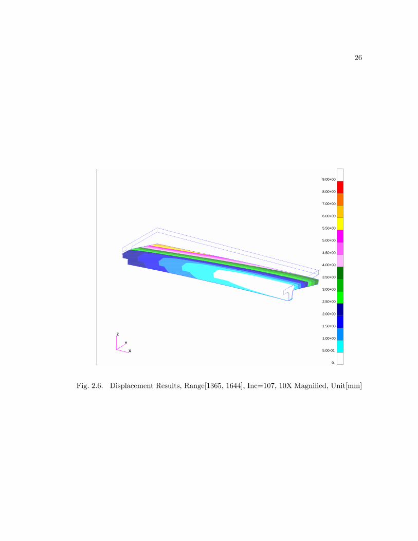
The mechanical analyses are also performed on this model to check the differ-

ence of distortions introduced by adopting these three different latent heat ranges. The

boundary conditions for mechanical analyses are shown in Figure 2.4. Symmetric bound-

ary conditions are applied on two symmetric planes with X and Y displacements fixed

respectively, and XYZ displacements of Node 1 are fixed. The final displacement results

are shown in Figure 2.5, Figure 2.6, Figure 2.7. The Z-displacement results along the

side of the plate, which is marked as Curve 1 in the model (Figure 2.4), are also recorded

in Figure 2.8 as a measure of welding introduced angular distortion. The total time

increment counts and the maximum absolute Z-displacement results (corresponding to

Node 2 in Figure 2.4) are recorded in Table 2.1.

Latent Heat Thermal Mechanical Max Z-displacement

[1415, 1594] 650 108 8.05 mm

[1365, 1644] 139 107 6.84 mm

[1315, 1694] 104 97 6.36 mm

Table 2.1. Time increment counts and maximum absolute Z-displacement results

25

X

Y

Z

9.00+00

8.00+00

7.00+00

6.00+00

5.50+00

5.00+00

4.50+00

4.00+00

3.50+00

3.00+00

2.50+00

2.00+00

1.50+00

1.00+00

5.00-01

0.

X

Y

Z

Fig. 2.5. Displacement Results, Range[1415, 1594], Inc=108, 10X Magnified, Unit[mm]

26

X

Y

Z

9.00+00

8.00+00

7.00+00

6.00+00

5.50+00

5.00+00

4.50+00

4.00+00

3.50+00

3.00+00

2.50+00

2.00+00

1.50+00

1.00+00

5.00-01

0.

X

Y

Z


27

X

Y

Z

9.00+00

8.00+00

7.00+00

6.00+00

5.50+00

5.00+00

4.50+00

4.00+00

3.50+00

3.00+00

2.50+00

2.00+00

1.50+00

1.00+00

5.00-01

0.

X

Y

Z


28

0. 1.50+02 3.00+02 4.50+02 6.00+02 7.50+02 9.00+02

-9.00+00

-7.50+00

-6.00+00

-4.50+00

-3.00+00

-1.50+00

0.

LEGEND

Length of Path (mm)

Dis

plac

emen

ts Z

(mm

)

Maximum ∆t=2.0s, Latent heat range [1315, 1694]



Fig. 2.8. Z Direction Displacement Results

29

From Table 2.1, it can be seen that expanding the latent heat range from [1415,

1594] to [1365, 1644] helps to reduce the time increment count from 650 to 139 in the

thermal analysis, which reduces computational time dramatically. The relative error

of the maximum absolute Z-displacement results between the latent heat range [1415,

1594] and [1365, 1644] is calculated in Equation (2.4). It shows that 15.0% of error is

introduced by this expanding procedure, which is worthwhile to compromise considering

that 78.6% of increments are saved.

error =8.05 − 6.84

8.05= 15.0% (2.4)

When the latent heat range is expanded further, from [1415, 1594] to [1315, 1694],

the time increment count is reduced from 650 to 104. However, the relative error of the

maximum absolute Z-displacement results increases to 21 % (computed based on the

same equation Equation (2.4), just change 6.84 to 6.36). Therefore, it is not worthwhile

to consider this expansion since the computational savings are not significant compared

to the previous case, and 6% more error is introduced.

Based on the above observations, the latent heat range is chosen to be [1365,

1644].

2.4.3 Spatial and Temporal Discretization Requirements

With the objective to reduce unnecessary computational costs as while as to

achieve sufficiently reliable results, minimum discretization requirements for modeling

welds should be satisfied [28]. In the Maglev beam model, the following spatial and

30

temporal discretization are used as a general rule to mesh all the welds and control

maximum time increment:

1. Four quadratic elements are included along each axis in the “double ellipsoid”

model [28].

2. The heat source may move approximately one-half of weld pool length in one time

step [28].

2.4.3.1 Maximum Time Increment (∆tmax

) for Thermal Analysis

The amount of time to be incremented at each time increment, ∆t, is controlled

by the predicted time increment ∆tpredict

(based on the error estimation result from the

last time increment) and also capped by ∆tmax

, as shown in Equation (2.5).

∆t = min(∆tpredict

, ∆tmax

) (2.5)

∆tmax

is computed from the above temporal discretization requirement as follows:

v × ∆tmax

≤ c for all welds (2.6)

where c is the weld ellipsoid length in Equation (2.3), it also approximates one-half

of weld pool length. v is the velocity of a specific weld. In the potential welding design of

the Maglev beam, c is around 20 mm and v varies from 2.1 mm/s to 10.8 mm/s. In the

current implementation, one value for ∆tmax

is used for all welds. Therefore, ∆tmax

is

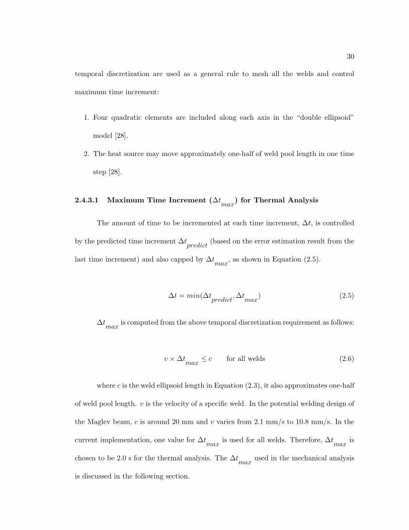
chosen to be 2.0 s for the thermal analysis. The ∆tmax

used in the mechanical analysis

is discussed in the following section.

31

2.4.3.2 Maximum Time Increment (∆tmax

) for Elasto-Plastic Mechanical

Analysis

The elasto-plastic mechanical analysis uses a quasi-static scheme, and several time

increments are computed to simulate the plasticity evolution resulting from the high

temperature results introduced in welding. Generally, the problem size in mechanical

analysis is three times of the problem size in thermal analysis, therefore much more com-

putational time is required for the mechanical analysis compared to that of the thermal

analysis. However, unlike the thermal analysis, where a strict temporal discretization

is required to correctly capture the heat input, ∆tmax

in the elasto-plastic mechanical

analysis can be expanded to reduce the total computational time.

∆tmax

in the mechanical analysis is also weld dependent. Generally, ∆tmax

should be tested and validated through numerical experiments performed on the weld

with the lowest torch travel speed, since for welds with high torch travel speeds, ∆tpredict

will be used as the time increment amount, and ∆tmax

will not take effects (see Equation

(2.5)).

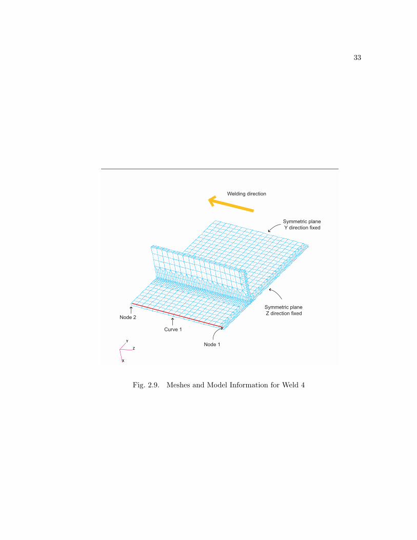
Another small welding model based on weld 4 in the Maglev beam model is built

and shown in Figure 2.9. This weld connects the bulkhead to the webplate, and it has

the lowest torch travel speed among all welds, v = 2.17 mm/s. The welding heat input

is Qw

= 2930 W , and the welding efficiency is η = 0.8.

Elasto-plastic mechanical analysis with ∆tmax

=2.0 s and ∆tmax

=5.0 s are per-

formed and compared on this small welding model. The dimensions of this model are as

follows: length of the plate=572.23 mm, width of the plate=1073 mm, thickness of the

32

plate=12.26 mm, height of the stiffener=182.80 mm, thickness of the stiffener=25 mm.

The total simulation time is 275 s, and the cooling process is simulated at the last time

increment by imposing the ambient temperature field on the structure.

The boundary conditions for the mechanical analyses are shown in Figure 2.9.

Symmetric boundary conditions are applied on two symmetric planes with Y and Z

displacements fixed respectively. Also the XYZ displacements of Node 1 are fixed. The

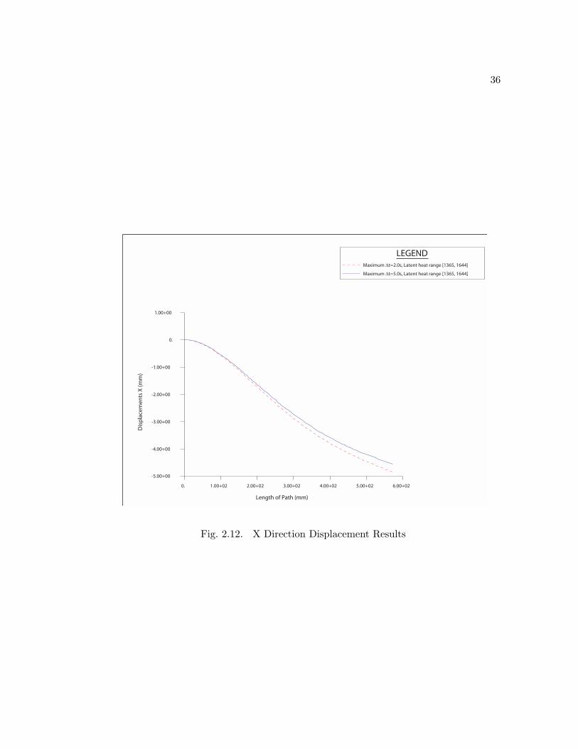
final displacement results are shown in Figures 2.10 and 2.11. The X-displacement along

Curve 1 is plotted in Figure 2.12. The total time increment counts and maximum X-

displacement results (corresponding to Node 2 in Figure 2.9) are recorded in Table 2.2.

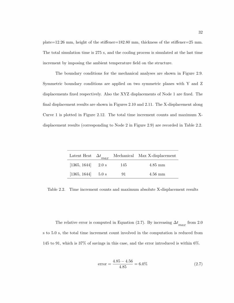
Latent Heat ∆tmax

Mechanical Max X-displacement

[1365, 1644] 2.0 s 145 4.85 mm

[1365, 1644] 5.0 s 91 4.56 mm

Table 2.2. Time increment counts and maximum absolute X-displacement results

The relative error is computed in Equation (2.7). By increasing ∆tmax

from 2.0

s to 5.0 s, the total time increment count involved in the computation is reduced from

145 to 91, which is 37% of savings in this case, and the error introduced is within 6%.

error =4.85 − 4.56

4.85= 6.0% (2.7)

33

X

Y

Z

X

Y

Z

Symmetric plane

Z direction fixed

Curve 1

Node 2

Welding direction

Symmetric plane

Y direction fixed

Node 1

Fig. 2.9. Meshes and Model Information for Weld 4

34

X

Y

Z

5.20+00

4.80+00

4.40+00

4.00+00

3.60+00

3.30+00

3.00+00

2.40+00

2.10+00

1.80+00

1.50+00

1.20+00

9.00-01

6.00-01

3.00-01

0.X

Y

Z

Fig. 2.10. Displacement Results, ∆tmax

= 2.0s, Inc=145, 10X Magnified, Unit[mm]

35

X

Y

Z

5.20+00

4.80+00

4.40+00

4.00+00

3.60+00

3.30+00

3.00+00

2.40+00

2.10+00

1.80+00

1.50+00

1.20+00

9.00-01

6.00-01

3.00-01

0.X

Y

Z

Fig. 2.11. Displacement Results, ∆tmax

= 5.0s, Inc=91, 10X Magnified, Unit[mm]

36

0. 1.00+02 2.00+02 3.00+02 4.00+02 5.00+02 6.00+02

-5.00+00

-4.00+00

-3.00+00

-2.00+00

-1.00+00

0.

1.00+00

LEGEND

Length of Path (mm)

Dis

plac

emen

ts X

(mm

)



Fig. 2.12. X Direction Displacement Results

37

Therefore, in the final elasto-plastic mechanical analysis of the Maglev beam

model, the maximum time increment ∆tmax

is chosen to be 5.0 s.

2.5 The Full Scale Maglev Beam Model

The Maglev Pennsylvania Project [42] plans to deploy high-speed maglev trains

in commercial service with an initial project forty to fifty miles in length. It provides

a possible alternate source of transportation that offers competitive trip-time savings to

auto and aviation modes in the 40- to 600-mile travel markets. Magnetic forces are used

to suspend, guide and propel the vehicles on the guideway. There are no wheels, no

moving parts and no physical contact with the guideway. Therefore, there is no friction

and wear on moving parts. The absence of contact results in an exceptional ride quality

for the passenger, very quiet operation and reduced maintenance costs.

The Maglev system is designed to operate at speeds in excess of 310 mph, and the

Maglev beam is one important integral component of the transrapid guideway. The over-

all system ride comfort is directly related to the execution and quality of the guideway.

Therefore guideway specifications and tolerances are especially important. The guide-

way structure must be manufactured within very small tolerances. The 47-mile proposed

Pennsylvania alignment consists of over 2000 guideway beams, each measuring 203 feet

long, weighing 135 tons with compound curves built-in and having to be manufactured

within millimeters of tolerance. Along the top plate, the tolerance is ±5 mm, and on

the critical surfaces (stator and guidance magnets), the tolerance is ±2 mm. Precision

fabrication technology needs to be developed for the production of the guideway beam

within specifications.

38

2.5.1 Model Information and Welding Conditions

Figure 2.13 shows a section of the Maglev guideway beam, which is one of the main

components of the magnetic levitation transportation system. The guideway beam is

double span and is supported by piers with varying distances between them depending on

the beam type and curvature. The section of a beam known as the Type 1 guideway beam

is analyzed in this work. As shown in Figure 2.13, the guideway beam is a trapezoidal

box beam structure with 25 mm thick stiffeners located at fixed intervals. The main

components are the top flange (deck plate, 18 mm thick), the side web plates (12 mm

thick) and the bottom flange (lower chord, 40 mm thick). The top flange, side web plates

and bottom flange are welded longitudinally using fillet welds. The stiffeners are welded

onto the top flange using double fillet welds.

The actual length of the main guideway beam utilized in this project is 61.92

m. As the beam has a uniform cross section and consists of alternating diaphragm and

crossbeam stiffeners at equally spaced intervals of approximately 3 m, only a portion

of the beam is analyzed to simplify the analysis. A 6.88 m long portion that contains

two bulkhead stiffeners and one crossbeam stiffener, as shown in Figure 2.13, is planned

for instrumented testing. However, in the numerical simulations, the 6.88 m model is

still too large and exceeds the computer resource limitations. Therefore, a model which

represents 1/8 portion of the 6.88 m Maglev beam is built for simulation purpose, which

is shown in Figures 2.15 and 2.16.

There are in all ten types of welds that are considered for this analysis. Their

processing paths are shown in Figure 2.14 and the detailed information is listed below.

39

Deck Plate 18mm

Guidance Rail 30mm

Web Plate 12mm

Lower Chord 40mm Stator Flange

25mm

Stator Web 15mm

Bulkhead 25mm

Inlet10mm

Cross Beam 25mm

Fig. 2.13. The Components of the Maglev Guideway Beam

40

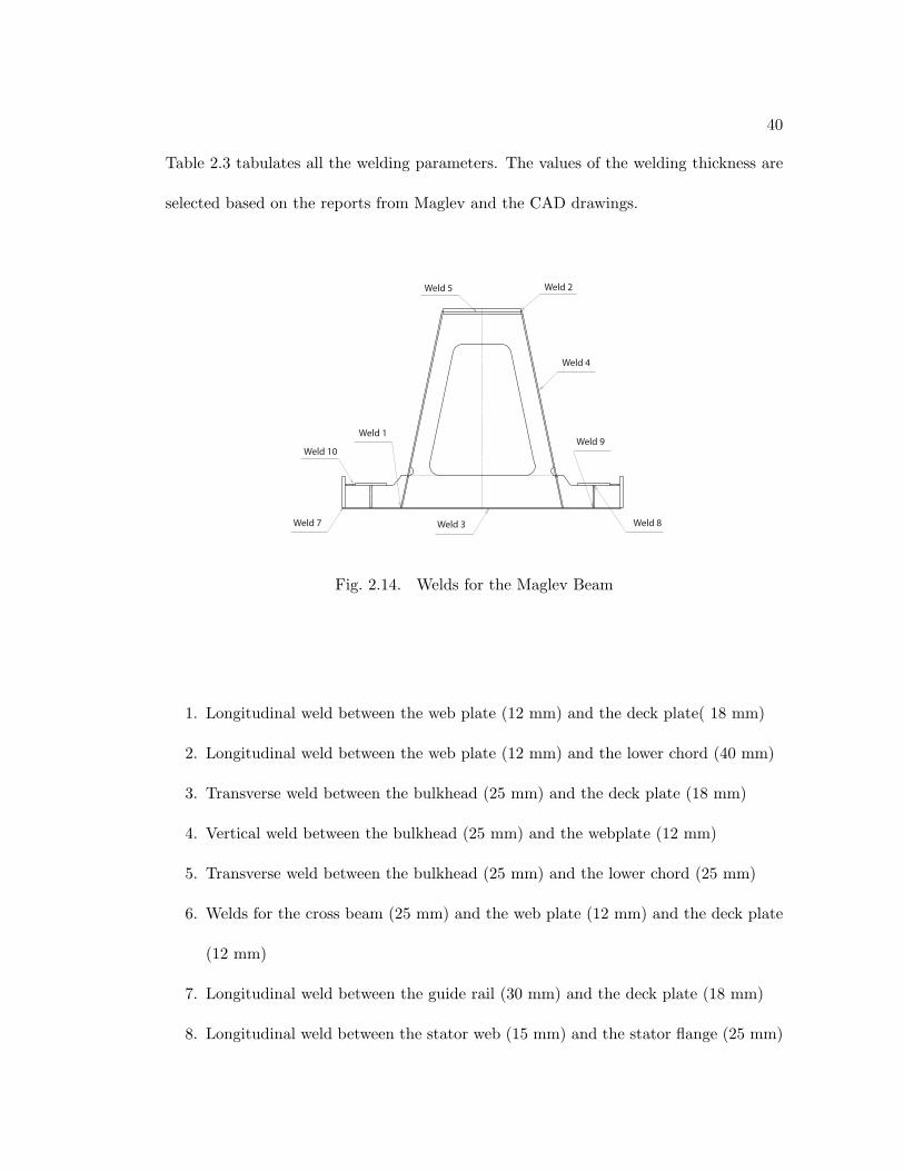
Table 2.3 tabulates all the welding parameters. The values of the welding thickness are

selected based on the reports from Maglev and the CAD drawings.

Weld 2

Weld 8Weld 7

Weld 1Weld 9

Weld 4

Weld 3

Weld 5

Weld 10

Fig. 2.14. Welds for the Maglev Beam

1. Longitudinal weld between the web plate (12 mm) and the deck plate( 18 mm)

2. Longitudinal weld between the web plate (12 mm) and the lower chord (40 mm)

3. Transverse weld between the bulkhead (25 mm) and the deck plate (18 mm)

4. Vertical weld between the bulkhead (25 mm) and the webplate (12 mm)

5. Transverse weld between the bulkhead (25 mm) and the lower chord (25 mm)

6. Welds for the cross beam (25 mm) and the web plate (12 mm) and the deck plate

(12 mm)

7. Longitudinal weld between the guide rail (30 mm) and the deck plate (18 mm)

8. Longitudinal weld between the stator web (15 mm) and the stator flange (25 mm)

41

9. Longitudinal weld between the stator web (15 mm) and the deck plate (18 mm)

10. Longitudinal weld between the inlets (10 mm) and the stator beam (25 mm) and

the guide rail (30 mm)

Case Type Thickness Volts Amps Travel Speed Wire Feed

mm inch/min inch/min

1 Horizontal fillet 8 29 340 15.3 500

2 Vertical fillet 8 25 125 5.0 160

3 Overhead fillet - 3 passes 8 24.5 125 10.2 160

4 Horizontal fillet 6 28 340 25.5 500

5 Vertical fillet 6 25 125 9.1 160

6 Overhead fillet 6 24.5 125 10 160

Table 2.3. Welding Parameters

2.6 Simulations and Results of the Maglev Beam Model

2.6.1 Model and Welds Information

The meshes of the Maglev beam model is shown in Figure 2.15. Two inlets are

included in this model. It consists of 84668 Hex20 elements and 424343 nodes. The

numbers of equations in thermal and mechanical analyses are listed in Table 2.4. The

42

dimensions of this large scale model are listed as follows: length=1894 mm, width=1385

mm, height=1994 mm. The total weld length in this model is 13.3 m. Symmetric

boundary conditions are applied on two symmetric planes with X and Y displacements

fixed respectively. Also the XYZ displacements of Node 1 are fixed. The welds are shown

in Figure 2.16 in red color and the boundary conditions are also included.

Thermal Analysis Mechanical Analysis

Total Equations 424343 1269792

Time Increments 1579 602

Wallclock Time 56 Hours 91 Hours

Table 2.4. Equations and Simulation Statistics for the Large Scale Model

The welds in the numerical simulation are performed in sequential order as listed

in Table 2.5. The timing information is also recorded for all the welds. The third column

in Table 2.5 records the total time duration of a specific weld, and the fourth column

records the start time of a specific weld.

All the welds finish at t=2678 s. In the simulation, 2800 s is computed. A follow

on Total Lagrange large deformation analysis is performed after the last time increment

of the elasto-plastic mechanical analysis to capture the possible buckling phenomenon.

43

X

Y

Z

X

Y

Z

Fig. 2.15. Meshes for Large Scale Maglev Model

44

X

Y

Z

X

Y

Z

Symmetric plane

X direction fixed

Symmetric plane

Y direction fixed

Node 1

Curve 1

Curve 2

Fig. 2.16. Welds and Boundary Conditions for the Large Scale Maglev Model

45

Number Weld Description Duration Start Time

1 The web plate to the deck plate 292s 0s

2 The guide rail to the deck plate 292s 292s

3 The stator web to the deck plate 175s 584s

4 The stator web to the stator flange 292s 759s

5 The inlets to the stator beam and the guide rail 98s 1051s

6 The web plate to the lower chord 175s 1149s

7 The bulkhead to the deck plate (inside box) 118s 1324s

8 The bulkhead to the web plate 130s 1442s

9 The bulkhead to the stator web 65s 1572s

10 The bulkhead to the stator flange 53s 1637s

11 The bulkhead to the deck plate (outside box) 101s 1690s

12 The bulkhead to the web plate 887s 1791s

Table 2.5. The Sequential Welds Information for the Large Scale Maglev Model

46

Cooling down is simulated by imposing the ambient temperature field on the model and

performing an additional large deformation analysis.

2.6.2 Thermal and Mechanical Results

The temperature results at increment 1501 (t=2645.20s) are shown in Figure 2.17.

The final large deformation displacement results at time increment 602 (t=2800.00s) are

shown in Figure 2.18. The small deformation results are almost the same as those from

the large deformation analysis, which implies there is no buckling after welding.

Curves 1 and 2 are marked along the guide rail (the dot lines in Figure 2.16),

and the X and Z direction displacement results of these two curves are recorded in

Figure 2.19, Figure 2.20, Figure 2.21 and Figure 2.22 for both the small and the large

deformation analysis. Some oscillation of the results along Curve 1 is observed, which is

caused by the weld performed along this curve. The results for the small and the large

deformation analysis are also very close to each other as shown in these figures.

The maximum absolute X and Z displacement results from the large deformation

analysis are shown in Table 2.6. The X displacement is primarily attributed to the

angular distortion, and its dependence on the length of the model is low. Therefore, the

angular distortion satisfies the ±2 mm design specifications. However, the Z displacement

is primarily attributed to longitudinal bowing distortion, and it is expected to increase

when the length of the model increases. To correctly predict this bowing distortion, a

larger model is needed to be built to verify the effect of model length on the bowing

distortion.

47

X

Y

Z

1.60+03

1.40+03

1.20+03

1.00+03

9.00+02

8.00+02

7.00+02

6.00+02

5.00+02

4.00+02

3.00+02

2.00+02

1.00+02

7.50+01

5.00+01

2.50+01

X

Y

Z

Fig. 2.17. Temperature Results of Large Scale Maglev Beam, t=2645.20s, Unit[oC]

Curve 1 Curve 2

X 0.18 mm 1.18 mm

Z 1.02 mm 0.95 mm

Table 2.6. Maximum Absolute X and Z Displacement Results, Large DeformationAnalysis

48

X

Y

Z

7.00+00

6.50+00

6.00+00

5.50+00

5.00+00

4.50+00

4.00+00

3.50+00

3.00+00

2.50+00

2.00+00

1.50+00

1.00+00

5.00-01

0.

X

Y

Z

Fig. 2.18. Displacement Results of 1/8 Maglev Beam, Large Deformation, t=2800.00s,50X Magnified, Unit[mm]

49

0. 3.50+02 7.00+02 1.05+03 1.40+03 1.75+03 2.10+03

0.

2.00-01

4.00-01

6.00-01

8.00-01

1.00+00

1.20+00

LEGEND

Dis

plac

emen

ts Z

(mm

)

Displacements Z, Small Deformation Analysis

Displacements Z, Large Deformation Analysis

Length of Path (mm)

Fig. 2.19. Z Direction Displacement Results of Curve 1 in Large Scale Maglev Beam,t=2800.00s

50

0. 3.50+02 7.00+02 1.05+03 1.40+03 1.75+03 2.10+03

-2.00-01

-1.60-01

-1.20-01

-8.00-02

-4.00-02

0.

4.00-02

LEGEND

Length of Path (mm)

Dis

plac

emen

ts X

(mm

)

Displacements X, Small Deformation Analysis

Displacements X, Large Deformation Analysis

Fig. 2.20. X Direction Displacement Results of Curve 1 in Large Scale Maglev Beam,t=2800.00s

51

0. 3.50+02 7.00+02 1.05+03 1.40+03 1.75+03 2.10+03

-2.00-01

0.

2.00-01

4.00-01

6.00-01

8.00-01

1.00+00

LEGEND

Dis

plac

emen

ts Z

(mm

)

Length of Path (mm)

Displacements Z, Small Deformation Analysis

Displacements Z, Large Deformation Analysis

Fig. 2.21. Z Direction Displacement Results of Curve 2 in Large Scale Maglev Beam,t=2800.00s

52

0. 3.50+02 7.00+02 1.05+03 1.40+03 1.75+03 2.10+03

-1.20+00

-1.00+00

-8.00-01

-6.00-01

-4.00-01

-2.00-01

0.

LEGEND

Length of Path (mm)

Dis

plac

emen

ts X

(mm

)

Displacements X, Small Deformation Analysis

Displacements X, Large Deformation Analysis

Fig. 2.22. X Direction Displacement Results of Curve 2 in Large Scale Maglev Beam,t=2800.00s

53

2.6.3 Performance Results

The simulation is performed on the 16 CPU Unisys ES7000 system. Time incre-

ments and wallclock time statistics of the thermal and elasto-plastic mechanical analyses

are listed in Table 2.4. Speedup is also measured on an 8 CPU SGI Altix 350 system for

the first 38 time increments based on the wallclock time spent on a single CPU, which

is shown in Table 2.7. 3.94 is achieved for the thermal analysis and 4.51 is achieved for

the mechanical analysis.

Thermal Analysis (s) Mechanical Analysis (s)

1 CPU 81302 171397

8 CPUs 20645 37967

Speedup 3.94 4.51

Table 2.7. Speedup Results Based on Wallclock Time, First 38 Time Increments

2.7 Conclusions and Future Work

This paper investigates the deployment of parallel computing and serval related

modeling and optimization issues used for simulating welding distortion in large struc-

tures. The FEA algorithm is also carefully implemented on a large shared memory

54

computer and optimized to achieve the optimal computational performance. The op-

timized approach is applied on the large scale Maglev beam problem with 1.27 million

equations, and the computational statistics demonstrate that this approach provides a

feasible way to simulate large scale welding applications in a short amount of time, which

are thought to be a very computationally challenging problem during the last decades.

Future work will focus on the following two topics: The first topic is to implement

different maximum time increment values ∆tmax

for different welds, therefore to further

improve the overall computational efficiency. The second topic is to build a twice longer

Maglev beam model compared to the one used in this paper, and investigate the effect

of model length on the bowing distortion.

55

Chapter 3

A Fast Implementation of the FETI-DP Method:

FETI-DP-RBS-LNA and Applications on Large Scale

Problems with Localized Nonlinearities

3.1 Introduction

In many science and engineering disciples, such as, material processing, biome-

chanics and structural dynamics, large scale finite element simulations are heavily desired

with the objective to correctly simulate full scale physical processes and achieve high fi-

delity numerical results. The total number of finite element equations arising from these

problems can be in the millions. Solving these large scale problems poses many challenges

for currently available numerical algorithms as well as computer hardware.

Extensive research has been conducted to develop an efficient and reliable nu-

merical method that is capable of solving large scale problems. Direct sparse solvers

are recognized as robust and efficient and are already employed in many commercial fi-

nite element softwares. However, the high memory demands and the not-so-well parallel

scalability [43] of direct sparse solvers restrict their applications to large scale prob-

lems. Traditional iterative solvers are excellent from the memory point of view and

can be easily parallized. However, they are problem dependent in some cases, and for

ill-conditioned engineering problems, they are not as reliable as direct sparse solvers.

2The content of this chapter has been published on International Journal for Numerical Meth-ods in Engineering. Volume 63, Issue 6, Pages: 833-858.

56

One alternative choice is the Domain Decomposition (DD) style methods which com-

bine advantages of both direct and iterative solvers. The DD methods are based on

the divide-and-conquer concept. They distribute the computational tasks based on the

splitting of a large geometric domain into several subdomains with either overlapping or

non-overlapping interfaces, and then these subdomains can be submitted to individual

computing nodes and processed in a parallel fashion. For the DD methods with non-

overlapping interfaces, two parallel approaches that implement the DD algorithms have

been studied intensively. Based on parameters chosen on interfaces to keep the continuity

of neighboring subdomains, these two approaches are named as the primal substructur-

ing method and the dual substructuring method, respectively. Taking solid mechanics

problems as an example, the primal substructuring method chooses displacements as in-

terface unknowns [44, 45, 46], and one example is the Balancing Domain Decomposition

method (BDD) proposed by Mandel [47]. The dual substructuring method chooses in-

terface forces, which are resembled by Lagrange multipliers, as unknowns, and the FETI

family algorithms belong to this category [48, 49, 35].

The original Finite Element Tearing and Interconnecting method (FETI) was first

introduced by Farhat and Roux [48, 50, 51, 52, 53]. A set of Lagrange multipliers λ is

introduced to enforce the continuity of neighboring subdomains. This set of Lagrange

multipliers, together with the coefficients of rigid body modes for floating subdomains,

form the basic unknowns of the interface equation. This interface equation is solved by

the preconditioned conjugate projected gradient method (PCPG). The optimal conver-

gence properties for second order elliptic problems, such as plain strain/stress problems

and solid mechanics problems discretized by brick elements, are studied in references

57

[54, 55, 56]. When equipped with the mechanically consistent Dirichlet preconditioner

[54] and applied to second order elliptic problems, it shows the condition number of

interface equation κ, grows asymptotically as

κ = O(1 + log2(

H

h)) (3.1)

where H is the subdomain size and h is the mesh size. The condition number κ is weakly

related to the values of H and h, and this property results in good numerical and parallel

scalability of the FETI method, which is shown on a 1000-processor configuration of the

ASCI Option Red supercomputer at Sandia National Laboratory [57]. For fourth order

plate and shell problems, the original FETI method is no longer numerically scalable.

The two-level FETI method (FETI-2) is developed to solve these types of problems [49,

58, 59]. The FETI-2 method introduces an additional set of Lagrange multipliers at the

subdomain corners, and determines their values at each PCG iteration through solving

the coarse problem formed by the subdomain rigid body modes and the subdomain corner

modes. This additional procedure enforces the continuity of the transverse displacements

at the subdomain corners and improves the scalability of fourth order plate and shell

problems. When the Dirichlet preconditioner is used, the condition number estimate,

which is Equation (3.1), still holds for its interface equation [60].

The new generation of FETI family methods, the Dual-Primal FETI method

(FETI-DP) [34, 35] preserves the satisfactory numerical and parallel scalability of the

original FETI and FETI-2 methods for second and fourth order problems. It also uses

Lagrange multipliers to place the continuity constraints on interfaces. However, instead

58

of introducing the coefficients for rigid body modes in the original FETI and the second

set of Lagrange multipliers in FETI-2, it chooses some corner node degrees of freedom as

basic unknowns so that each subdomain is non-singular. Thus it circumvents solving all

the rigid body modes and the generalized inverse of the subdomain matrices. The coarse

problems of FETI-DP, which are essential for scalability properties, in general, are also

sparser than those of FETI and FETI-2. These features make FETI-DP much more uni-

form and applicable for programming than its predecessors, and numerical experiments

show that it also delivers better computational performance under most circumstances

[34]. The FETI family of algorithms has been implemented for problems arising from

many engineering fields [61, 62, 63, 64, 65, 66, 67, 68, 69, 70, 71]. When some modi-

fications are made to solve multiple right hand sides [72, 73], this method can also be

applied in sensitivity analysis, optimization and design fields [74].

One important feature of domain decomposition (DD) based iterative solvers with

a direct sparse solver as the local solver is that more CPU time is spent in local back-

substitutions than in local factorizations. In the FETI family of algorithms, many local

back-substitutions are involved in the step of solving large interface problems iteratively

by the PCG method, and these local back-substitutions consume a high percentage of

the total CPU time. Some detailed CPU measurement results can be found in reference

[66] and the welding example in this paper. If the Dirichlet preconditioner is applied,

many additional local back-substitutions will also be involved. The total number of lo-

cal back-substitutions is also related to the precision requirement of the results. It takes

more PCG iterations, and therefore more local back-substitutions, to achieve higher

precision results. To alleviate this computational difficulty, a reduced back-substitution

59

(RBS) algorithm is proposed in this paper based on investigations of the boolean ma-

trices involved in these back-substitutions. The RBS algorithm performs a reordering

of the equations and removes unnecessary computations performed on equations that

are not needed in back-substitutions. Therefore, this algorithm reduces the size of back-

substitution problems, and considerable computational time is saved. Overhead from

numeric factorizations will be introduced due to this specific ordering strategy. This

overhead is problem dependent, and in general, related to the way that meshes and sub-

domains are generated. However, for large scale problems with localized nonlinearities,

this overhead is acceptable and does not prevent savings of overall CPU costs since when

linear-nonlinear analysis (LNA) is applied, which will be discussed in the next paragraph,

only a few nonlinear subdomains require re-factorizations.

The built-in divide-and-conquer concept of DD methods also benefits large scale

problems with localized nonlinearities. The well-known linear-nonlinear analysis (LNA)

can be adopted to reduce unnecessary computations in the numeric factorizations of

linear subdomains. This results in significant reduction of computational time for large

scale problems with localized nonlinearities, such as welding problems. In this paper, the

FETI-DP-RBS-LNA method, which combines FETI-DP, RBS and LNA, is proposed to

solve large scale problems with localized nonlinearities. This approach is demonstrated

on a welding problem. The welding simulations are known to be very computationally

expensive due to the dense meshes and small time increments required to correctly cap-

ture the moving heat source inputs and the resulting high gradient temperature and

residual stresses fields [28]. One numerical experiment is performed on a 16-subdomain

hollow beam welding model with a total of one million degrees of freedom. The serial

60

CPU time on an Unisys ES7000 system is measured for the IBM Watson Sparse Matrix

Package (WSMP) [36, 37], the FETI-DP algorithm and the FETI-DP-RBS-LNA algo-

rithm. The CPU results show that the FETI-DP-RBS-LNA algorithm outperforms both

of them in this case.

In the following paragraphs, section 2 presents a review of the general frame-

work of the FETI-DP algorithm. Section 3 proposes the RBS algorithm and discuss its

advantages and disadvantages. Section 4 reviews the main concept of linear-nonlinear

analysis (LNA) and provides specific linear-nonlinear identification criteria for thermal

and mechanical analyses in welding problems. Section 5 presents the serial CPU time

and memory costs of the mechanical analyses for a 16-subdomain hollow beam welding

problem. Finally, section 6 concludes the paper and suggests several future work.

3.2 Review of The FETI-DP Method

3.2.1 Saddle Point of the Lagrangian

The foundation of the FETI family methods for three dimensional linear elasto-

static problems is to solve the saddle point of the following Lagrange function in Equation

(3.2), and detailed explanation of this idea and definitions of terms are in [48, 51].

J∗(v1

, v2, ..., v

s, µ) =

ns∑

i=1Ji(vi) +

nl∑

l=1(vi − v

j, µ)

Γl (3.2)

61

The solutions u1, u

2, ..., u

s and interface forces λ for the above problem should

satisfy the saddle point equations derived from Equation (3.2), which are listed in Equa-

tion (3.3) for future reference.

∂J∗(u1

,u2,...,u

s,λ)

∂ui = 0 i = 1, 2, ..., ns

∂J∗(u1

,u2,...,u

s,λ)

∂λ = 0

(3.3)

3.2.2 Matrix Formulations

In this section, the FETI-DP method are reviewed and the matrix formulations

are presented, most of them can be found in the related papers, for example [34]. They

are presented to provide reference for later discussions.

In Figure 3.1, a large domain Ω is divided into four subdomains and finite element

discretization is applied. The subdomain related nodes are classified into three groups

based on their locations. They are corner nodes, non-corner interface nodes and internal

nodes, respectively. For a specific subdomain, the global stiffness matrix Ks, solution

vector us and load vector f

s can be rearranged as the format of Equation (3.4) based

on the above nodes classification.

Ks =

Ks

iiK

s

ibr

Ks

ibc

Ks

ibr

TK

s

brbr

Ks

brbc

Ks

ibc

TK

s

brbc

TK

s

bcbc

us =

us

i

us

br

us

bc

fs =

fs

i

fs

br

fs

bc

(3.4)

62

Ω1

Ω

Ω

Ω

2

3

4

Corner Nodes Non-Corner Interface Nodes Internal Nodes

Fig. 3.1. Subdomains with non-overlapping interfaces, their meshes and nodes classifi-cation

63

where s corresponds to subdomain index, i stands for the internal node degrees of free-

dom, bc

is the corner node degrees of freedom, and br

refers to the non-corner interface

node degrees of freedom.

There are several definitions of corner nodes, and the choice of corner nodes

will affect the size of the coarse problem, which is essential for parallel scalability of

the FETI-DP method [34, 35]. It will also affect the convergence speed of the PCG

method for interface problems. In Ref [34], the corner nodes are defined as: c1) The

points belonging to more than two subdomains, and c2) The set of nodes located at

the beginning and end of each edge of each subdomain. Defining all the nodes in group

c1 to be corner nodes is important since these nodes do not belong to any interfaces

between two subdomains. Thus they cannot be simply replaced by normal Lagrange

multipliers λ. The corner nodes in group c2 are required to remove the rigid body modes

of subdomains. Noticing that both primal unknowns u and dual unknowns λ are used in

the FETI-DP interface equations and they are interchangeable on non-corner interface

degrees of freedom, except the above two groups, some additional corner nodes can be

added to replace the previous non-corner interface nodes without alternating the FETI-

DP algorithm. This modification could reduce the PCG iteration count for applications

with relatively large local subdomain problems and relatively small coarse problems,

since more corner nodes help to ”fix” each subdomain and accelerate convergence.

The global vector of corner degrees of freedom, each individual subdomain non-

corner degrees of freedom and subdomain interface degrees of freedom are defined in

64

Equation (3.5):

uc

=

u1

c

u2

c...

uN

cc

us

r=

us

i

us

br

u

s

b=

us

br

us

bc

(3.5)

Two additional mapping matrices, as shown in Equation (3.6), are introduced to

map degrees of freedom between these vectors. Here Bs

rare signed boolean matrices,

and the sign is defined as follows: For each degree of freedom (equation) on the interface

of subdomain i and j, if the corresponding component in Bi

ris first set to be +1, then

the corresponding component in Bj

rwill be −1, and vise versa. B

s

care normal boolean

matrices. During the computations, the mapping actions of these boolean matrices and

their transposes on a vector perform scatter and gather operations instead of any real

matrix-vector multiplications.

Bs

rus

r= ±

0

...

us

br

...

0

and Bs

cuc

= us

bc

(3.6)

With all these definitions, through a standard Galerkin procedure to discretize

Equation (3.3) and after several rearrangements of the terms, the dual-primal interface

65

equation for the FETI-DP method is listed in Equation (3.7):

FIrr

FIrc

FIrc

T −K∗cc

λ

uc

=

d

r

−f∗c

(3.7)

where

FIrr

=

ns∑

s=1B

s

rK

s

rr

−1B

s

r

T (3.8)

FIrc

=

ns∑

s=1B

s

rK

s

rr

−1K

s

rcB

s

c(3.9)

K∗cc

= Kcc

−n

s∑s=1

(Ks

rcB

s

c)T K

s

rr

−1(Ks

rcB

s

c) (3.10)

dr

=

ns∑

s=1B

s

rK

s

rr

−1fs

r(3.11)

f∗c

= fc−

ns∑

s=1B

s

c

TK

s

rc

TK

s

rr

−1fs

r(3.12)

Kcc

=

ns∑

s=1B

s

c

TK

s

ccB

s

c(3.13)

Noticing that Equation (3.7) is based on both primal unknowns uc

and dual

unknowns λ. When the dimension of λ reduces to zero, all dual unknowns are replaced

by primal unknowns. This equation becomes a pure primal substructuring interface

equation, which is Equation (3.14), where K∗cc

is just the Schur complement matrix in

66

the traditional domain decomposition method.

K∗cc

uc

= f∗c

(3.14)

Conversely, if the dimension of uc

reduces to zero, all the primal unknowns are

replaced by dual unknowns. Equation (3.7) becomes the original FETI interface equation

without any constrains of rigid body motions, which is shown in Equation (3.15).

FIrr

λ = dr

(3.15)

Eliminating uc

from the dual-primal interface equation, Equation (3.7), yields

Equation (3.16) about Lagrangian multipliers λ on interfaces:

(FIrr

+ FIrc

K∗cc

−1F

Irc

T )λ = dr− F

Irc

K∗cc

−1f∗c

(3.16)

This is the interface equation that needs to be solved first in the FETI-DP algo-

rithm. The computation of K∗cc

−1, which is used in the right hand side, is referred to as

the coarse problem of the FETI-DP method. A short summary of solution procedures

of the FETI-DP method is listed in Table 3.1. The equation in step S3 for solving the

rest subdomain internal unknowns us

rcan be derived directly from the discretized form

of Equation (3.3). For solid mechanics problems and thermal problems with constant

conductivity, since their stiffness matrices are symmetric positive definite (SPD), the

matrix (FIrr

+FIrc

K∗cc

−1F

Irc

T ) in the interface equation, Equation (3.16), is also SPD.

The PCG method provides an efficient choice to solve this type of equations.

67

S1. Solve the interface unknowns λ from Equation (3.16)(F

Irr

+ FIrc

K∗cc

−1F

Irc

T )λ = dr− F

Irc

K∗cc

−1f∗c

S2. Solve the corner nodes unknowns uc

from Equation (3.7)

uc

= K∗cc

−1(f∗c

+ FIrc

Tλ)

S3. Solve the subdomain internal unknowns us

rfrom

us

r= K

s

rr

−1(fs

r− K

s

rcB

s

cuc− B

s

r

Tλ)

Table 3.1. Solution Procedures of the FETI-DP Method

To reduce the iteration count in the PCG iterations, refinement of the FETI-DP

algorithm is possible by enforcing an optional admissible constraint in Equation (3.17)

at each PCG iteration [34]. This accelerates the convergence rate if the full column rank

matrix Q is properly chosen. rk is a residual associated with the dual interface problem

and has the form of Equation (3.18). It stands for the difference of u on the interfaces

between neighboring subdomains, and will approach zero when the interface equation

converges. The details of augmented equations can be found in [34].

QT

rk = 0 (3.17)

rk = d

r− F

Irc

K∗cc

−1f∗c− (F

Irr

+ FIrc

K∗cc

−1F

Irc

T )λk =

ns∑

s=1B

s

rusk

r(3.18)

68

3.2.3 Preconditioners and Conjugate Gradient Method

The Dirichlet and lumped preconditioners used here are extended from those in

the original FETI and FETI-2 methods [34]. The Dirichlet preconditioner is defined as:

FD

Irr

−1=

ns∑

s=1w

sB

s

r

0 0

0 Ss

brbr

B

s

r

Tw

s (3.19)

where Ss

brbr

are Schur complement matrices:

Ss

brbr

= Ks

brbr

− Ks

ibr

TK

s

ii

−1K

s

ibr

(3.20)

and the lumped preconditioner is:

FL

Irr

−1=

ns∑

s=1w

sB

s

r

0 0

0 Ks

brbr

B

s

r

Tw

s (3.21)

where ws are scaling diagonal matrices that account for eventual subdomain hetero-

geneities [75], and they are chosen to be identity matrices I in the numerical experi-

ments in this paper. The Dirichlet preconditioner is more computationally expensive

than the lumped preconditioner since it involves numeric factorizations of Ks

iiand back-

substitutions solving Ks

ii

−1β for each subdomain during each PCG iteration. However,

in general, it reduces the required iterations and improves the overall computational

69

efficiency for fourth order plate and shell problems, and the lumped preconditioner is

mostly used for second order problems [34].

The details of the PCG algorithm can be found in [76, 34]. In general, the relative

residual is used to predict when to exit PCG iterations, which is shown in Equation (3.22).

‖ Ku − f ‖2‖ f ‖2

≤ ε (3.22)

3.3 Reduced Back-Substitution Algorithm

The PCG iterations for large interface problems are found to be the time con-

suming part in the FETI family algorithms. Within the PCG costs, a high percentage

of the CPU time is actually consumed by the local back-substitutions inside the PCG

iterations. The detailed percentage mainly depends on the size of the coarse problem,

the number of subdomains, and the running mode of the program (serial or parallel

mode). Some examples of CPU usage statistics can be found in Ref [66] and the welding

simulation problem in this paper. For the diffraction grating problem and the alloy wheel

problem in Ref [66], when a sparse solver is used for the local factorizations, the local

back-substitutions consumes 55.3% and 69.2 % of the total CPU time, respectively. For

the mechanical analysis of the welding problem in this paper, which stands for a cate-

gory of applications with small coarse problems, Figure 3.2 shows the serial CPU costs of

local factorizations, PCG and local back-substitutions in the FETI-DP algorithm, and

the local back-substitutions consumes 64.3% of the total CPU time.

70

From a mechanical point of view, local back-substitutions are essential to find

the interface forces that ”glue” the previous discrepancy displacement fields on the in-

terfaces, which is shown in Equation (3.18). The relationship between interface forces

and interface displacements is mathematically represented by the inverses of subdomain

stiffness matrices, and these local back-substitutions help to solve the global interface

forces based on the difference of displacements on interfaces. On the other hand, local

back-substitutions are also involved in preconditioning the system, as shown in Equation

(3.20).

Back-Substitutions within PCGPCGNumeric Decomposition

Fig. 3.2. Serial CPU Costs of FETI-DP

Therefore, local back-substitutions play an important role in the FETI-DP al-

gorithm, and since they consume a high percentage of the CPU time, the reduction of

computations in these steps will greatly improve the overall performance of the FETI-DP

algorithm. In this section, the computations in the back-substitution steps are carefully

investigated. The matrices and right hand side vectors involved in the equations are

properly reordered to reduce the computations in these steps.

71

3.3.1 Sparsity and Reduced Back-Substitutions in PCG

During each PCG iteration, the most time consuming steps are calculating the

following two matrix-vector multiplications listed in Equation (3.23). Each multiplication

has several back-substitutions involved.

(FIrr

+ FIrc

K∗cc

−1F

Irc

T ) · λ and FD

Irr

−1 · λ (3.23)

Now, taking one sub-step from the first multiplication FIrr

·λ as an example, and

substituting the detailed expression of FIrr

, it yields the following equation:

FIrr

· λ =

ns∑

s=1B

s

rK

s

rr

−1B

s

r

Tλ (3.24)

In the standard FETI-DP method, Bs

r

Tλ is calculated first and then K

s

rr

−1(Bs

r

Tλ)

is solved as a whole through the back-substitution, where Ks

rr

−1 is the inverse of subdo-

main matrix which has already been decomposed and stored in previous steps. Finally,

the solution vector Ks

rr

−1(Bs

r

Tλ) is multiplied by the mapping matrix B

s

ragain to form

Bs

r(Ks

rr

−1(Bs

r

Tλ)), and summed over all the subdomains. The reason this process re-

quires so much time lies in the relatively large number of equations in each subdomain, as

the back-substitution is actually performed on each subdomain internal and non-corner

interface degrees of freedom (equations). The left part of Figure 3.3 shows the nodes

involved in this standard back-substitution.

In the following paragraphs, a reduced back-substitution (RBS) algorithm is pro-

posed to reduce the unnecessary equations involved in the back-substitutions and save

72

computational costs. Notice Bs

rare signed boolean matrices which map the internal

and non-corner interface degrees of freedom in each subdomain to the global non-corner

interface degrees of freedom, which is shown in Equation (3.25). It can be seen that

only in the row and column corresponding to us

bri∗

, the component of Bs

ris +1 or −1.

Elsewhere it is always 0. Although Equation (3.25) (also the coming Equation (3.26) and

Equation (3.28)) is listed in the format of matrix-vector multiplications, it just serves to

help understanding. In actual numerical applications, scatter and gather operations are

taken instead of multiplications.

Bs

rus

r=

0 ... 0 0 ... 0

......

......

......

0 ... 0 ±1 ... 0

......

......

......

0 ... 0 0 ... ±1

......

......

......

0 ... 0 0 ... 0

us

i1...

us

in

us

bri1...

us

brim

=

0

...

±us

bri1

...

±us

brim...

0

(3.25)

When Bs

r

T is applied on λ through scatter operations to calculate Bs

r

Tλ in Equa-

tion (3.24), only the components corresponding to non-corner interface equations of sub-

domain s are extracted out and assigned a sign. Other components in the result Bs

r

Tλ

will be 0 regardless of what they are in the original λ. Thus, if the equations corre-

sponding to non-corner interface degrees of freedom are reordered and numbered last,

the detailed expression of this scatter operation can be written as in Equation (3.26),

73

Standard Back-Substitution Involves Non-Corner Interface Nodes and Internal Nodes

Reduced Back-Substitution Involves OnlyNon-Corner Interface Nodes


Fig. 3.3. Nodes Involved in Standard Back-Substitution and Reduced Back-Substitutionfor Subdomain Ω2 in Figure 3.1

74

and the ”±” sign means either ”+” or ”−” will be chosen for a specific component in λ.

Bs

r

Tλ =

0

...

0

±λ1...

±λm

= γ (3.26)

In the result vector γ, only the values in the last m positions, which corresponds

to non-corner interface degrees of freedom, are non-zeros.

Assuming the subdomain stiffness matrices Ks

rrare symmetric positive definite,

Cholesky factorization is performed on each subdomain, as shown in Equation (3.27).

Ks

rr= L

sL

sT (3.27)

Once Ks

rr

−1B

s

r

Tλ, name it β here, is computed, B

s

rK

s

rr

−1B

s

r

Tλ is calculated

by applying Bs

ron K

s

rr

−1B

s

r

Tλ through gather operations. It also only extracts the

components corresponding to non-corner interface equations of subdomain s, which is

already clustered at the last m positions of vector Ks

rr

−1B

s

r

Tλ. This procedure and the

75

final result are shown in Equation (3.28).

Bs

rK

s

rr

−1B

s

r

Tλ = B

s

rβ = B

s

r

∗...

∗

β1...

βm

=

0

...

±β1...

±βm

...

0

(3.28)

From the above analysis, it can be seen that, when performing the back-substitutions,

if the equations corresponding to non-corner interface degrees of freedom are reordered

and numbered last, due to the scatter and gather operations of Bs

r

T and Bs

r, only the

last m components from λ are required as input for the back-substitutions, and only the

last m components from the back-substitution result Ks

rr

−1B

s

r

Tλ are required as output

to compute Equation (3.24). Thus the back-substitution is actually performed on the

last m equations. The value of m is equal to the number of the subdomain non-corner

interface degrees of freedom. m is much smaller than the sum of subdomain internal

degrees of freedom and non-corner interface degrees of freedom. Therefore, much time

can be saved based on this reduced back-substitution (RBS). The nodes involved in this

RBS algorithm are shown in the right part graph of Figure 3.3. Compared to standard

back-substitution, many internal nodes are not necessary to be included anymore.

76

The above analysis also results in that only part of the Ls matrices will be used

in the RBS algorithm. Carefully looking at the Cholesky factorization of the subdomain

stiffness matrices Ks

rr= L

sL

sT , after the reordering, the Ls matrix can be written as:

Ls =

ls

i1 ,1

ls

i2 ,1

ls

i2 ,2

......

. . .

ls

bri1 ,1

· · · · · · ls

bri1 ,b

ri1...

......

.... . .

ls

brim ,1

· · · · · · ls

brim ,b

ri1

· · · ls

brim ,b

rim

(3.29)

Now the problem is to solve the last m components of β = Ks

rr

−1γ, and γ has the

non-zero structure as shown in Equation (3.26). It involves solving a two step forward

and backward substitution problem, which is shown in Equation (3.30).

LsL

sTβ = γ → L

sξ = γ & L

sTβ = ξ (3.30)

Since only the last m components of γ are non-zeros, instead of the entire Ls

matrix, only the right-down part of Ls matrix, which is from row b

ri1to b

rimand

column bri1

to brim

, is used to solve the intermediate result ξ from the forward back-

substitution in Equation (3.30). Name the right-down part of Ls matrix as L

s

br

, and

77

now ξ also has the similar non-zero structure as γ, which is shown in Equation (3.31):

ξ =

0

...

0

ξ1...

ξm

(3.31)

The next step is to solve LsT

β = ξ. Since only the last m components of β are

needed, it is easy to see that the submatrix Ls

br

T already contains enough information

to solve this. Although there are many non-zeros left unsolved in β, their results are not

required since Bs

rwill mask them out later.

Therefore, the entire RBS algorithm for the computation of Equation (3.24) can

be summarized as follows:

1) For each subdomain, the equations related with non-corner interface degrees

of freedom are first reordered after all other equations in this subdomain.

2) Based on this restriction, the proper ordering scheme is applied and the sub-

domain stiffness matrices Ks

rrare factorized. The factorized matrices information is

stored.

3) Later, when performing the back-substitutions, only part of the factorized

matrices information, which is Ls

br

, will be reused.

78

For the rest of back-substitutions in matrix-vector multiplications in Equation

(3.23), most of them are the same as the above example, while some are slightly different

since they are also affected by the corner nodes, such as the following example:

FIrc

· ξ =

ns∑

s=1B

s

rK

s

rr

−1K

s

rcB

s

cξ (3.32)

Under these circumstances, only a little modification on ordering is required. For

all the nodes that belong to the same element with the corner nodes, their equations

also need to be renumbered last. The reason behind that is that matrix Ks

rcis a sparse

matrix and plays a similar role to that of Bs

r

T .

However, there is one exception that cannot benefit from this improved algorithm.

For back-substitutions listed in Equation (3.33) below, which are used in Equation (3.11)

and Equation (3.12) in the FETI-DP algorithm, the above scheme cannot be applied since

fs

rdoes not follow the structure of γ as in Equation (3.26).

ψ = Ks

rr

−1fs

r(3.33)

From a solid mechanics point of view, back-substitutions in Equation (3.33) are

all necessary for general problems with body forces. They help to introduce the external

loads to each subdomain, and these loads may not be simplified into terms on interfaces.

Fortunately, these back-substitutions only require to be computed once and take quite

little CPU time (less than two percent for the testing case in this paper during the entire

PCG iterations), so that they will not affect the overall improvement.

79

It must be mentioned that the proposed reduced back-substitutions will affect

the ordering scheme since it poses the restriction to re-number the related equations to

the end of the entire equations. This re-numbering introduces additional time costs in

the numeric factorization stage compared to the situation with a good ordering scheme,

such as the nest-dissection scheme. This overhead is related to the ratio of subdomain

interface equations with respect to subdomain total equations, and it is also related to

the general sparse pattern of the matrices to be factorized. Therefore, the overhead

really varies from problem to problem, and its value can range from 0.5 to 4 times the

costs of numeric factorization with a good ordering scheme. In general, finding a good

cut of the domain that generates small interfaces will help to reduce this overhead. In

case of applications with small coarse problems and localized nonlinearities, such as the

welding problem in this paper, the subdomains only need to be factorized a few times,

and the increased overhead will become trivial since more time is saved from the reduced

back-substitutions.

3.3.2 Mathematical Analysis of Computational Costs

Based on the RBS algorithm, the equations involved in back-substitutions are re-

duced to subdomain non-corner interface equations only. Unlike the FETI-DP method,

back-substitutions are performed on subdomain internal and non-corner interface equa-

tions. Assuming the number of subdomain internal equation is Ns

i, the number of

subdomain non-corner interface equations is Ns

br

, and the total number of equations is

Ns = N

s

i+ N

s

br

.

80

Fig. 3.4. Triangulation of Square Mesh

A simple two dimensional K × K triangulation square mesh with one degree of

freedom per node is used as the analytical model to provide some mathematical insight

of the costs from standard and reduced back-substitutions, which is shown in Figure 3.4.

The total number of equations in this model is Ns = K × K.

1) Standard back-substitution:

Standard finite element problems generally use the nested dissection scheme to

order their matrices. Based on the analysis from George, Liu and Ng [77], the number

of fill-in non-zeros in Ls introduced after Cholesky factorization for the above model is:

|Ls| =314

O(K2log2K) + O(K2) (3.34)

Since the back-substitution is performed on the entire Ls matrix, its cost is ap-

proximate to the non-zeros involved. Therefore it is 314 O(K2

log2K) + O(K2).

81

2) Reduced back-substitution:

All the interface (boundary) equations are ordered after the rest of internal

equations, and only the small portion of Ls matrix, which is L

s

br

, is used for back-

substitutions. The number of interface equations is O(K). For a regular subdomain

discretized by the finite element method, through the fill path theorem [78], a path with

lower order numbers exists to connect any two interface nodes, thus this factorized Ls

br

matrix is a dense matrix. Therefore the total number of non-zeros inside is:

|Ls

br

| = O(K × K) = O(K2) (3.35)

Now the back-substitution cost is around O(K2).

From the above analysis, when the RBS algorithm is applied to this 2D model,

the back-substitution costs are reduced from 314 O(K2

log2K) + O(K2) to O(K2) in this

case. For problems involved with many back-substitutions, considerable computational

time can be saved. If the problem has smaller interfaces with respect to the size of the

subdomain, more savings can be expected.

3.4 Large Scale Analysis of Welding Problems

Finite element formulations for quasi-static thermo-elasto-plastic processes in La-

grangian reference frames have been widely used in analyzing fusion welding processes

[30, 16, 9, 8, 21, 31, 26, 3]. The thermal analysis is assumed to be transient while the

elasto-plastic mechanical analysis is quasi-static. Thermo-elasto-plastic processes are

typically assumed to be weakly coupled; that is, the temperature profile is assumed to

82

be independent of stresses and strains. Thus, a heat transfer analysis is performed ini-

tially and the resulting temperature history is imported as the thermal loading in the

following mechanical analysis. Both the thermal and mechanical analyses are nonlinear

problems due to the temperature dependent material properties. Furthermore, plasticity

introduces additional sources of nonlinearity in the mechanical analysis.

For industry applications, the finite element welding simulations are computa-

tionally very expensive due to the following reasons:

1) They are large scale problems. Since near the thermal processing path, very

dense meshes are required to capture the high gradient temperature and residual stresses

results [28], which increases the size of the problem dramatically. For large scale appli-

cations, it is common that the total number of equations may exceed a million.

2) Small time increments are required to capture the moving heat input correctly

[28]. For simulations with several meters of welding, hundreds and even thousands of

time increments may be required.

3) Part of the structure behaves nonlinearly. In the standard direct method, this

behavior will require the entire system to be re-factorized for each Newton-Raphson

iteration in each time increment, increasing the already expensive computation costs.

Several approaches have be studied with the objective to solve this type of large

scale problems. One of them is adaptive meshing [32, 33]. This approach automatically

refines or coarsens the meshes along the welding path based on the temperature or stress

gradient, thus it reduces the unnecessary mesh density and saves computational time.

However, due to the high gradient residual stresses in regions previously processed ther-

mally, coarsening is still a problem in mechanical analysis since dense meshes are still

83

required to capture these high gradient residual stresses and strains, and these resid-

ual stresses and strains play important roles in the structural distortions. Therefore, in

mechanical analysis, adaptivity can only take full effect in regions that have not been

processed. This limits the effectiveness of adaptive meshing. Another approach is the do-

main decomposition method discussed in the previous section. By splitting a large scale

problem into many small problems, the domain decomposition method improves compu-

tational efficiency by reducing the problem size and using parallel computing techniques.

Both are essential for solving large scale problems.

3.4.1 Review of Thermal and Mechanical Analytical Formulations

3.4.1.1 Transient Thermal Analysis

In transient thermal analysis, for a reference frame r fixed to the body of a

structure, at time t, the governing equation for transient heat conduction analysis is

given as follows:

ρCp

∂T


where ρ is the density of the flowing body. Cp

is the specific heat capacity. T is the



frame r.



84

3.4.1.2 Quasi-Static Mechanical Analysis

In quasi-static mechanical analysis, the stress equilibrium equation is given as

follows:




be also found in most of the standard textbooks. Detailed formulations of small defor-

mation thermo-elasto-plasticity analysis can be found in [31].

3.4.2 Linear-Nonlinear Analysis with FETI-DP

Linear-nonlinear analysis (LNA) is a well-known concept to solve problems with

localized nonlinearity. It exploits information about which subdomain (substructure)

remains linear during a nonlinear analysis. Therefore, repeated factorizations of linear

subdomains can be avoided and computation costs can be saved.

The FETI-DP method provides a flexible option for handling subdomains sep-

arately, depending on their specific linear-nonlinear properties. Although the partial

derivative equations, as shown in Equation (3.3), are derived based on the linear elasto-

static assumption, their matrix formulations also hold for nonlinear elasto-plastic prob-

lems. This is because when the Newton-Raphson method is used to solve nonlinear

problems, during each iteration, the system to be solved is actually a linearized system.

For large scale problems with localized nonlinearities, linear-nonlinear analysis

can be very useful and save much computational time. Taking a welding problem in

85

small deformation analysis as an example, since welding heat input is concentrated in a

small region, nonlinearity is also a local phenomenon and most of the regions that are

far away from the weld behaves linearly in the welding process.

During a Newton-Raphson iteration, the matrices to be factorized in the FETI-DP

method are:

K1

rr, K

2

rr, ... , K

n

rrand K

1

ii, K

2

ii, ... , K

n

ii(3.38)

where the first n matrices are for interface equations, and the next n matrices are for

the Dirichlet preconditioner. For a general problem, all the subdomain stiffness matrices

are required to be re-factorized, so that the interface equation, which is Equation (3.16),

can be formed and the local results can be calculated as in Table 3.1. This process

can be greatly simplified through linear-nonlinear analysis, as long as the nonlinearity is

predictable before each factorization.

In the FETI-DP-RBS-LNA algorithm, since only a few subdomains need to be

re-factorized, linear-nonlinear analysis also reduces the overhead results from numeric

factorizations that require a special ordering scheme. Therefore, large scale problems

with locolized nonlinearity can be solved efficiently by using this algorithm.

Based on the implicit solution scheme using the Newton-Raphson method, linear-

nonlinear analysis can be applied to the following two situations: 1) the non-first Newton-

Raphson iterations and 2) the first Newton-Raphson iteration. In both situations, local

86

subdomain residual check is used as the criteria to identify linear and nonlinear subdo-

mains. The main difference between these two types of situations is: In the first Newton-

Raphson iteration, the residual result is not known and a testing iteration should be

performed to check the residual for each subdomain. In the non-first Newton-Raphson

iteration, the residual result for each subdomain is already known from the previous

Newton-Raphson iteration, and it can be used to identify the linear or nonlinear subdo-

main.

3.4.3 Criteria to Identify Linear and Nonlinear Subdomains

3.4.3.1 Criteria for the Non-First Newton-Raphson Iterations

For transient thermal and quasi-static elasto-plastic mechanical analyses in weld-

ing problems, it is convenient to check the nonlinearity for the non-first Newton-Raphson

iterations by examining its local residual Rs. This criterion is due to the fact that a

linear subdomain will converge after the first iteration, therefore its residual will become

zero, and a nonlinear subdomain will not converge after the first iteration, therefore it

will have a non-zero residual. For a thermal analysis, this residual is formed on the r

type of degrees of freedom, which include 1) internal node degrees of freedom, plus 2)

non-corner interface node degrees of freedom. For a mechanical analysis, this residual

is formed on the internal node degrees of freedom and excludes any degrees of freedom

from the nodes that belong to the same element with the corner nodes.

87

Through finite element formulations, the standard residual R in thermal analysis

can be derived as in Equation (3.39) [31].

R( nT) =∑V

BT kB nT − NT

Q + NT NρCp

nT − n−1Tnt − n−1t

WJ +

∑A

q

NTqwj (3.39)

where left superscript n represents quantities evaluated at the time increment of nt.

N and B are shape function matrices which interpolate the temperature T and the

temperature gradient ∇T within an element. J and j are the volume and area Jacobian

component corresponding to the Gaussian weighting W for volume and w for surface

integration. Aq stands for surfaces with prescribed heat fluxes q.

However, when a domain is decomposed into several subdomains, for residual Rs

of each subdomain, one additional term Fs should be added to represent heat fluxes

from the neighboring subdomains, which is shown in Equation (3.40).

Rs( nT) = R( nT) + Fs( nT), where Fs( nT) = −Ks

rcBs

cu

c− Bs

r

Tλ (3.40)

where −Ks

rcBs

cu

cstands for the contribution from corner node temperature u

c, and

−Bs

r

Tλ stands for the contribution from interface flux λ.

The residual Rs of each subdomain in mechanical analysis can be derived as in

Equation (3.41) [31].

Rs( nU) =∑V

BT n

σ − NT b

WJ −∑A

t

NT twj (3.41)

88

where t are the prescribed tractions on surface At.

In a non-first Newton-Raphson iteration, if the computed Rs is less than or equal

to some predefined tolerance tolRt

for the thermal analysis and tolRm

for the mechanical

analysis, as shown in Equation (3.42), then the related subdomain s is identified as a

linear subdomain, and no re-factorization is required.

||Rs|| ≤ tolRt

||Rs|| ≤ tolRm

(3.42)

3.4.3.2 Criteria for the First Newton-Raphson Iterations

For both thermal and mechanical analyses during the first Newton-Raphson it-

eration, the above residual criteria can still be applied to identify linear and nonlinear

subdomains. However, one testing iteration using the old stiffness matrices from the last

time increment is required to obtain the residual result for each subdomain. The linear-

nonlinear identification decision for each subdomain is still made based on Equation

(3.42). If one subdomain requires re-factorization, the numerical results from this test-

ing iteration are discarded, and the program is reset to the initial state of this new time

increment. Re-factorizations of the identified nonlinear subdomains will then proceed.

However, due to the high computational costs of one testing iteration, in practice,

the criteria to identify nonlinear subdomains for the first Newton-Raphson iterations is

to check the change of the primary temperature field of each subdomain. If the change of

the primary temperature field is less than or equal to tolT

, as shown in Equation (3.43),

then the change of the subdomain stiffness matrix, which is related to the temperature

89

dependent material, can be ignored, and no re-factorization is required.

‖Ts|t=t

i+1

− Ts|

t=ti

‖ ≤ tolT

(3.43)

All these tolRt

, tolRm

and tolT

defined above can have different values for different

subdomains, based on their locations and effects upon the global solution precision.

In addition, this is a flexible way to control how often numeric factorizations should

be performed for different parts of the structure in the global time scale. When the

tolerances are set to be large values, less numeric factorization will be performed, and

the method behaves like a modified Newton-Raphson method.

The detailed FETI-DP-RBS-LNA algorithm is listed in Table 3.2. For a direct

sparse solver based algorithm, the steps from 2.1.1 to 2.1.4 will be replaced by a re-

factorization and a back-substitution of the whole system.

3.5 Large Scale Applications and Performance Results

3.5.1 Software and Hardware

The FETI-DP-RBS-LNA algorithm has been integrated into an in-house finite

element code which is capable of analyzing thermo-elasto-plastic problems. The code is

developed in Fortran 90. Modules are implemented for shared use of data and definitions.

Memory is efficiently utilized through dynamic allocation and deallocation. The IBM

Watson Sparse Matrix Package (WSMP) [36, 37] is implemented for subdomain level

factorizations, standard back-substitutions and reduced back-substitutions. Basic Linear

Algebra Subprograms (BLAS) are used to improve the performance of basic vector and

90

1. Preprocessing

Generate subdomains, mark corner nodes and non-corner interface nodes,

assemble stiffness matrices, perform ordering and symbolic factorization

2. Loop over time increments inc = 1, 2, 3...

2.1 Loop over the Newton-Raphson iterations iter = 1, 2, 3...

2.1.1 If inc = 1 and iter = 1

factorize all the matrices Ks

rrand, Ks

ii(for Dirichelt preconditioner)

Otherwise

only re-assemble and re-factorize nonlinear subdomain matrices

2.1.2 Call PCG solver to solve interface equation on λ

2.1.3 Solve corner results and each subdomain results

2.1.4 Form global residual R

2.1.5 If R < tolerance

go to step 2 and start a new time increment

Otherwise

go to step 2.1 and start a new Newton-Raphson iteration

Until all time increments are finished

Table 3.2. The FETI-DP-RBS-LNA Algorithm for Multi-time Increments NonlinearProblems

91

matrix related operations. The implementation uses the Intel Math Kernel Library

(MKL), version 7.0. The coarse problem, since it is quite small for the welding problem

in this paper, is currently stored in a dense format and solved by calling Intel MKL

functions dpotrf and dpotrs. Buffered writes are used to improve the efficiency of disk

I/O when the hard disk is non-local.

The simulations are performed on an Unisys ES7000 system. The system is 16-

way SMP based on 64-bit Intel Itanium2 processors, with 6 MB cache each. For the

performance tests in this paper, only one CPU is used to measure the serial CPU costs.

Shared memory is 32 GB and clock is 1.5 GHz per CPU. The OS is RedHat Enterprise

3 Linux, and the compiler is Intel ifort, version 8. The non-local hard disk access is via

NFS.

3.5.2 16-Subdomain Hollow Beam Model and Simulation Information

The 16-Subdomain hollow beam model, as shown in Figure 3.5, is chosen to

be the large scale welding problem for performance measurements in this paper. The

geometric dimensions of this model are listed as follows: height=2000 mm, width=2000

mm, length=1440 mm, thickness=20 mm. Hex20 elements are used in meshing. The

problem requires four welds with the same velocity v=6.5 mm/s in Z direction to be

performed along the corners of the beam in a sequential fashion.

Only the performance in the mechanical analysis is measured. For the thermal

analysis, since in this case, the conductivity of the material is temperature dependent.

Therefore the thermal problem is not SPD and FETI-DP can not be applied. Due to

the computer resource availability and time limits, the first 50 time increments of the

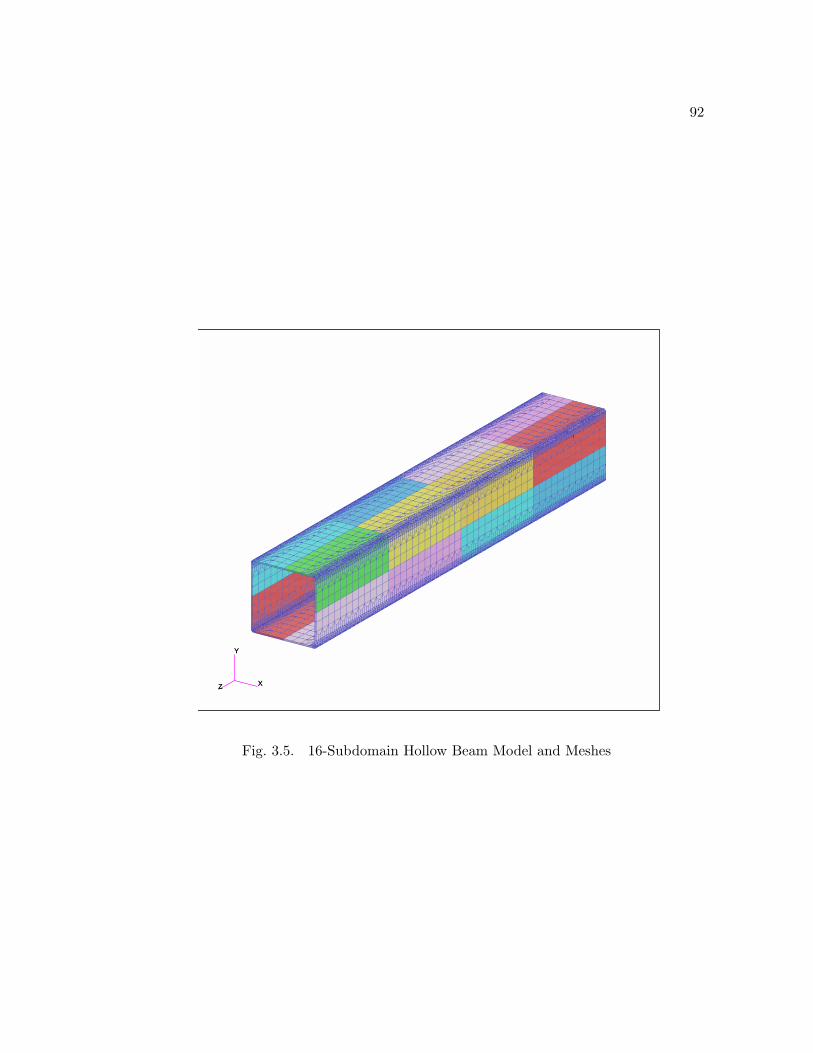
92

X

Y

Z X

Y

Z

Fig. 3.5. 16-Subdomain Hollow Beam Model and Meshes

93

mechanical analysis are computed. The finite element information and FETI-DP related

numbers of interface and corner equations are listed in Table 3.3.

Mechanical Analysis

Hex20 Element 65664

Total Equations 1007634

Interface Equations 8460

Corner Equations 174

Table 3.3. Finite Element and FETI-DP Information

Transient thermal analysis is performed initially by using the Goldak’s “double

ellipsoid” model to represent the welding heat input, as shown in Equation (3.44) [11].

Q =6√

3Qw

ηf

abcπ√

π[e−3((x

a )2+(yb )2+(z+vt

c )2)] (3.44)

where Qw

is the welding heat input, η is the welding efficiency, x, y, and z are the local

coordinates of the double ellipsoid model aligned with the weld fillet, a is the weld width,

b is the weld penetration, c is the weld ellipsoid length, v is the torch travel speed. In the

simulation, the following values are used: Qw

=8925 W, η=0.8, a=b=12.2 mm. Before

the torch passes the analysis plane, c=a and f=0.6. After the torch passes the analysis

plane, c=4a and f=1.4.

94

The material used in the welding simulations is A36 steel. The temperature

dependent thermal conductivity K and specific heat Cp

are based on the data in [39],

and the density of the steel is 7.82 × 103 kg/m3. The latent heat of fusion is set to be

247 kJ/kg/oC [40] and the ambient (room) temperature is set to be 25 oC.

During the simulation, relative residual tolerance ε for the PCG method, as shown

in Equation (3.22), is set to be 10−6. For LNA in the mechanical analysis, The following

values are set to identify linear and nonlinear subdomains, as shown in Equation (3.45)

tolRm

= 10−2tol

T= 102 (3.45)

3.5.3 Serial CPU Performance and Memory Results

The serial CPU costs of the IBM Watson direct sparse solver, FETI-DP, FETI-

DP-RBS, FETI-DP-LNA and FETI-DP-RBS-LNA in the mechanical analysis are mea-

sured and compared in Table 3.4, where NF is the step 2.1.1 in Table 3.2 and PCG

includes the steps from 2.1.2 to 2.1.4. The back-substitution costs in the PCG itera-

tions are also listed separately to show the improvement of the RBS scheme. In all FETI

schemes, Dirichlet preconditioner is used to preconditioning the system.

Figure 3.6 and Figure 3.7 show that, in the mechanical analyses, only the small

region along the welding path is affected by the changing temperature field and plasticity

phenomenon. Thus, LNA can be applied based on the criteria given in Equation (3.45)

to reduce re-factorizations.

During the initialization and ordering stage, which is shown in the first row in

Table 3.4, FETI-DP and its implementations with RBS or/and LNA take more time

95

X

Y

Z

1.00+03

9.00+02

8.00+02

7.00+02

6.00+02

5.00+02

4.50+02

4.00+02

3.50+02

3.00+02

2.50+02

2.00+02

1.50+02

1.00+02

5.00+01

2.50+01

X

Y

Z

Fig. 3.6. Temperature Results, Inc=51, Time=98 s, Unit[oC]

96

X

Y

Z

1.70-02

1.50-02

1.30-02

1.20-02

1.10-02

1.00-02

9.00-03

8.00-03

7.00-03

6.00-03

5.00-03

4.00-03

3.00-03

2.00-03

1.00-03

0.

X

Y

Z

Fig. 3.7. Equivalent Plastic Strain Results, Inc=51, Time=50 s

97

CPU Time (s) Serial Direct FETI-DP FETI-DP FETI-DP FETI-DP

Sparse Solver RBS LNA RBS & LNA

IO & SF 42.11 81.45 103.58 80.99 103.58

NF 47262.12 26525.69 40601.13 1849.01 2582.91

BS 1273.22 — — — —

PCG (LBS) — 58759.03 8879.37 58335.77 8900.07

— (54880.92) (5083.20) (54497.29) (5110.52)

TOTAL 48577.45 85366.17 49584.08 60265.77 11586.56

IO : Initialization and Ordering

SF : Symbolic Factorization

NF : Numeric Factorization

BS : Back-Substitution

PCG : Preconditioned Conjugate Gradient Iterations

(LBS) : Local Back-Substitution in PCG

LNA : Linear-Nonlinear Analysis

RBS : Reduced Back-Substitution

Table 3.4. Mechanical Analysis Serial CPU, First 50 Time Increments

98

compared to the direct sparse solver. This is because additional costs are spent on the

preconditioners, and with RBS, some overhead will also be introduced. However, the

CPU costs in this stage is trivial compared to that of the whole scheme, and they will

not affect overall performance.

During the numeric factorizations stage, which is shown in the second row in

Table 3.4, it can be seen that the FETI-DP method saves 44% of CPU time compared

to the direct sparse solver. This is because the direct sparse solver does not scale so well

when the size of the problem increases. When RBS is implemented, 53% of overhead

is introduced compared to the FETI-DP algorithm. However, LNA greatly reduces this

cost. Compared to the FETI-DP algorithm, 93% and 90% of CPU time are saved in the

FETI-DP-LNA implementation without RBS and with RBS, respectively.

During the preconditioned conjugate gradient iterations, as shown in the fourth

and fifth row in Table 3.4, RBS reduces 91% of CPU time for local back-substitutions,

and results in 85% of savings during the whole PCG iterations.

The total CPU costs are shown in the last row in Table 3.4. For this welding

problem with 16 subdomains, during the first 50 time increments, FETI-DP-RBS-LNA

improves the computational speed 4.2 times compared to the direct sparse solver and

7.4 times compared to the FETI-DP algorithm in the serial running mode.

However, since 16 may not be the optimal number of subdomains to deliver the

best performance of the FETI-DP algorithm, the CPU comparison results are just used to

test the LNA and RBS algorithms. Investigation of the speedup related to the FETI-DP

algorithm with optimal number of subdomains is beyond the scope of this paper. Also,

during the first 50 time increments, only one subdomain is identified to be nonlinear.

99

In the full simulation, the LNA CPU costs in numeric factorizations can be expected to

increase when more subdomains are identified to be nonlinear.

The memory statistics are also listed in Table 3.5. Since additional Dirichlet pre-

conditioners are required to be factorized, FETI-DP consumes more memory compared

to the direct sparse solver. The specific ordering scheme of RBS also introduces 11% of

overhead compared to the FETI-DP method in memory usage. However, this can be

resolved since in distributed computing environment, clusters can provide more memory.

Serial Direct FETI-DP FETI-DP FETI-DP FETI-DP

Sparse Solver RBS LNA RBS & LNA

Memory (Gb) 9.8 16.8 18.6 16.8 18.6

Table 3.5. Mechanical Analysis Memory Costs

3.6 Conclusion and Future Work

In this paper, a fast implementation of the FETI-DP algorithm: the FETI-DP-

RBS-LNA algorithm is proposed for solving large scale problems with localized nonlin-

earity. RBS is based on the motivation to reduce CPU costs in many time consuming

back-substitutions involved in the PCG iterations. Through a specific ordering, RBS

reduces the equations involved in the back-substitutions, thus it improves computational

100

speed. LNA is also adopted based on the nature of problems with localized nonlinearity.

It reduces numeric factorizations through a pre-identification procedure of subdomains,

and it also reduces the overhead arising from the specific RBS ordering scheme. This

combined approach can reduce CPU costs effectively.

Currently, the FETI-DP-RBS-LNA algorithm is tested in the serial running mode

with the objective to give a correct estimation of floating point performance. For parallel

and distributed architectures, it can also be implemented in a similar way as the FETI-

DP method. However, difficulty may arise from load balancing due to LNA. Although

the current FETI-DP-RBS-LNA algorithm may not reduce the total computational time

for one job , when multiple jobs are submitted to a parallel or distributed system, the

overall efficiency of the system will still be improved since the LNA scheme reduces the

total computations. Furthermore, two possible solutions to reduce this difficulty can be:

1) For large subdomains, calling an OpenMP version of solver in parallel environment

or an MPI version of solver in distributed environment to solve them. 2) For small

subdomains, redistributing subdomains need to be solved from heavy loaded CPUs or

computing nodes to less loaded CPUs or computing nodes, therefore to improve the

situation of load balancing.

The future work will be the distributed implementation of the FETI-DP-RBS-

LNA algorithm, and evaluation its performance in distributed computing environments.

101

Chapter 4

Distributed Computing with the FETI-DP-RBS-LNA

Algorithm on Large Scale Problems with

Localized Nonlinearities

4.1 Introduction

Large scale finite element analysis is an important research area due to its wide

applicability in modeling and simulating complicated scientific and engineering applica-

tions, such as structural mechanics, heat transfer, and biomechanics. For realistic and

sophisticated models, high density meshes are required to capture the underlying physics

in areas that are of particular interest or with complex geometry or loading. Accord-

ingly, the total degrees of freedom in systems discritized by the finite element method

may easily exceed a million, and it poses many computational challenges for current

available numerical algorithms as well as computer hardware.

Extensive research has been conducted to develop efficient and reliable numerical

methods which have the capabilities to solve large scale systems arising from various

disciplines. Two well-known approaches in this field are direct and iterative methods.

Direct sparse solvers are recognized as robust and efficient choices for most of the ap-

plications, and they are widely employed in many commercial finite element softwares.

However, the high memory demands and the not-so-well parallel scalability of direct

3The content of this chapter will be submitted to International Journal for Numerical Methodsin Engineering.

102

sparse solvers restrict its applications to large scale problems [43]. Traditional iterative

solvers are excellent from the memory point of view. However, they are problem de-

pendent and the convergence is not guaranteed. For complex ill-conditioned engineering

problems, they are not as reliable as direct sparse solvers.

Several novel approaches, such as Domain Decomposition (DD) methods, Adap-

tive meshing methods[32, 33], and Multigrid (MG) methods have also been studied

extensively for their possible applications to solve large scale systems. DD methods are

based on the native divide and conquer concept, they partition the physical domain into

subdomains with either overlapping or non-overlapping interfaces. Coarse-grain parallel

processing can then be applied to the computations of these subdomains to reduce overall

analysis time. Adaptive meshing refines or coarsens the meshes in different regions of the

model during the analysis based on their corresponding resolution requirements. There-

fore, this approach is capable to reduce the computational costs while still maintain the

quality of the solution. MG methods are based on the multilevel paradigm. They exhibit

optimal linear computational costs for some elliptic partial differential equations, such

as the Poisson’s equation. One extension of MG is Algebraic Multigrid method (AMG).

AMG constructs its operators directly from the sparse system matrix. Therefore, its ap-

plications are not limited by the geometry of the physical domains and it can be applied

to solve more general problems.

The objective of this paper is to present the FETI-DP-RBS-LNA algorithm [79]

and to investigate its distributed computing performance for large scale problems with

localized nonlinearity. The FETI-DP-RBS-LNA algorithm is based on one well known

DD style method: the Dual-Primal Finite Element Tearing and Interconnecting method

103

(FETI-DP)[34, 35]. Reduced Back-Substitution (RBS) algorithm is proposed to ac-

celerate costing local back-substitutions, and Linear and Nonlinear Analysis (LNA) is

introduced to reduce unnecessary re-factorizations of linear subdomains in the analysis.

The distributed version of this algorithm is implemented with Message Passing Inter-

face (MPI) and the performance is measured on a distributed PC cluster for a welding

mechanical analysis problem with approximate one million degrees of freedom.

4.2 Review of The FETI-DP-RBS-LNA Algorithm

4.2.1 The FETI-DP Algorithm

FETI-DP can be viewed as a combination of direct and iterative methods. Based

on the underlining divide and conquer concept, the physical domain is divided into

subdomains with non-overlapping interfaces. The related nodes after finite element dis-

cretization can be classified into three groups based on their locations, and they are

marked as corner nodes, non-corner interface nodes and internal nodes in Figure 4.1,

respectively. More details of FETI-DP can be found in Ref [79, 34, 35].

Through the similar concepts of super elements and substructures, the high level

interface problem can be first formulated and solved by an iterative Preconditioned

Conjugate Gradient (PCG) method. Once the interface solution is available, corner in-

formation can be further solved. After that, all the low level subdomains are independent

and can be solved by direct sparse solvers in a parallel fashion. These procedures are

shown in Figure 4.2.

104

Ω1

Ω

Ω

Ω

2

3

4


Fig. 4.1. Subdomains with non-overlapping interfaces, their meshes and nodes classifi-cation

Step 1 Solve Dual Interface Unknowns

(Non-corner Interface nodes)

Step 2 Solve Primal Corner Unknowns

(Corner nodes)

Step 3 Solve Primal Internal Unknowns

(Internal nodes)

Fig. 4.2. Solution Scheme of FETI-DP

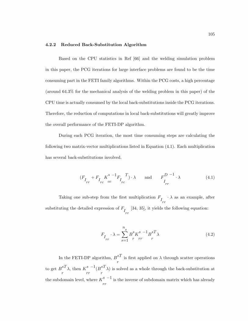
105

4.2.2 Reduced Back-Substitution Algorithm

Based on the CPU statistics in Ref [66] and the welding simulation problem

in this paper, the PCG iterations for large interface problems are found to be the time

consuming part in the FETI family algorithms. Within the PCG costs, a high percentage

(around 64.3% for the mechanical analysis of the welding problem in this paper) of the

CPU time is actually consumed by the local back-substitutions inside the PCG iterations.

Therefore, the reduction of computations in local back-substitutions will greatly improve

the overall performance of the FETI-DP algorithm.

During each PCG iteration, the most time consuming steps are calculating the

following two matrix-vector multiplications listed in Equation (4.1). Each multiplication

has several back-substitutions involved.

(FIrr

+ FIrc

K∗cc

−1F

Irc

T ) · λ and FD

Irr

−1 · λ (4.1)

Taking one sub-step from the first multiplication FIrr

· λ as an example, after

substituting the detailed expression of FIrr

[34, 35], it yields the following equation:

FIrr

· λ =

ns∑

s=1B

s

rK

s

rr

−1B

s

r

Tλ (4.2)

In the FETI-DP algorithm, Bs

r

T is first applied on λ through scatter operations

to get Bs

r

Tλ, then K

s

rr

−1(Bs

r

Tλ) is solved as a whole through the back-substitution at

the subdomain level, where Ks

rr

−1 is the inverse of subdomain matrix which has already

106

been factorized with its factorized information stored. Finally, Bs

ris applied on the

solution vector Ks

rr

−1(Bs

r

Tλ) through gather operations to form B

s

r(Ks

rr

−1(Bs

r

Tλ)) and

summed over all the subdomains. The reason this process requires much computational

time lies in the relatively large number of equations in each subdomain, as the back-

substitution is actually performed on each subdomain internal and non-corner interface

degrees of freedom (equations). The left part graph of Figure 4.3 shows the nodes

involved in this standard back-substitution.

Bs

r

T and Bs

rconnect subdomain level information to global domain information

through scatter and gather operations. If written in matrix format, their representations

are sparse matrices. Based on the analysis in Ref [79], assuming the number of equations

corresponding to non-corner interface degrees of freedom is m, and these equations are

numbered last. Only the last m components from λ are required as the input for the

back-substitutions in Equation (4.2) since Bs

rzeros the rest components, and only the

last m components from the back-substitution result Ks

rr

−1B

s

r

Tλ are required as the

output due to the same reason. Thus the back-substitution is actually performed on

the last m equations. m is a much smaller number compared to the sum of subdomain

internal degrees of freedom and non-corner interface degrees of freedom. Therefore, much

time can be saved based on this reduced back-substitution (RBS). The nodes involved

in this RBS algorithm are shown in the right part of Figure 4.3. Compared to standard

back-substitution, many internal nodes are not necessary to be included anymore.

It must be mentioned that the proposed reduced back-substitutions will affect

the ordering scheme since it poses the restriction to re-number the related equations to

the end of the entire equations. This re-numbering introduces additional time costs in

107

Standard Back-Substitution Involves Non-Corner Interface Nodes and Internal Nodes

Reduced Back-Substitution Involves OnlyNon-Corner Interface Nodes


Fig. 4.3. Nodes Involved in Standard Back-Substitution and Reduced Back-Substitutionfor Subdomain Ω2 in Figure 4.1

108

the numeric factorization stage compared to the situation with a good ordering scheme,

such as the nest-dissection scheme. This overhead is related to the ratio of subdomain

interface equations with respect to subdomain total equations, and it is also related to

the general sparse pattern of the matrices to be factorized. Therefore, the overhead

really varies from problem to problem, and its value can range from 0.5 to 4 times

the costs of numeric factorization with a good ordering scheme. In general, finding a

good decomposition of the domain that generates small interfaces will help to reduce this

overhead. In case of applications with small coarse problems and localized nonlinearities,

such as the welding problem in this paper, the subdomains only need to be factorized a

few times, and the increased overhead will become trivial since more time is saved from

the reduced back-substitutions.

4.2.3 Linear-Nonlinear Analysis

Linear-nonlinear analysis (LNA) is a well-known and efficient strategy to solve

problems with localized nonlinearity. It exploits information about which subdomain

remains linear during a nonlinear analysis. Therefore, repeated factorizations of linear

subdomains can be avoided and computation costs can be saved.

The FETI-DP method provides a flexible option for handling subdomains sepa-

rately. During a Newton-Raphson iteration, the matrices to be factorized in the FETI-

DP method are:

K1

rr, K

2

rr, ... , K

n

rrand K

1

ii, K

2

ii, ... , K

n

ii(4.3)

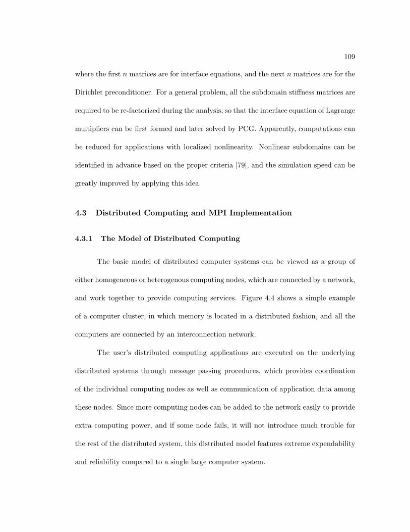
109

where the first n matrices are for interface equations, and the next n matrices are for the

Dirichlet preconditioner. For a general problem, all the subdomain stiffness matrices are

required to be re-factorized during the analysis, so that the interface equation of Lagrange

multipliers can be first formed and later solved by PCG. Apparently, computations can

be reduced for applications with localized nonlinearity. Nonlinear subdomains can be

identified in advance based on the proper criteria [79], and the simulation speed can be

greatly improved by applying this idea.

4.3 Distributed Computing and MPI Implementation

4.3.1 The Model of Distributed Computing

The basic model of distributed computer systems can be viewed as a group of

either homogeneous or heterogenous computing nodes, which are connected by a network,

and work together to provide computing services. Figure 4.4 shows a simple example

of a computer cluster, in which memory is located in a distributed fashion, and all the

computers are connected by an interconnection network.

The user’s distributed computing applications are executed on the underlying

distributed systems through message passing procedures, which provides coordination

of the individual computing nodes as well as communication of application data among

these nodes. Since more computing nodes can be added to the network easily to provide

extra computing power, and if some node fails, it will not introduce much trouble for

the rest of the distributed system, this distributed model features extreme expendability

and reliability compared to a single large computer system.

110

Memory

Processor

Memory

Processor

Memory

Processor

Memory

Processor


Distributed Computing on Distributed Memory Systems

Message Passing

Fig. 4.4. The Model of Distributed Systems

111

4.3.2 Message Passing Interface (MPI) Implementation

Message Passing Interface (MPI) is a library specification of message passing

for parallel computers and distributed clusters. It features with good scalability and

portability and has already been widely implemented by many applications in various

research area. In the current implementation, MPI is mainly implemented to distribute

computational loads in the following two tasks: 1) Subdomain level computations. 2)

The PCG solver used for solving the interface problems.

For the subdomain level computations, such as, forming the subdomain stiffness

matrices, local numeric factorizations, local back-substitutions and subdomain residual

computations, they can all be performed on each computing node in a distributed fashion.

A master computing node is assigned to read the input file and do preprocessing tasks

first, and MPI is implemented to pass the required subdomain geometry data, subdomain

finite element data and code internal control data from the master computing node to

the rest of computing nodes. For the PCG solver in the FETI-DP-RBS-LNA algorithm,

its main procedures are listed in Table 4.1, where Dirichlet preconditioner FD

Irr

−1is

chosen to preconditioning the system.

During the PCG iterations, there are several∑n

ss=1

operations which are per-

formed to sum up the results from all the sudomains, where ns

is the number of subdo-

mains. Currently, MPI collective communication calls MPI REDUCE are implemented to

gather the intermediate subdomain results, such as r0, z0 and zn, from each computing

node to the master computing node. The sum of these individual results are calculated

112

P1. Initialization

λ0 = 0

r0 = dr− F

Irc

K∗cc

−1f∗c

z0 = FD

Irr

−1r0

p0 = z0

c0 = z0T · r0

P2. Iterate n = 1, 2, 3, ... until residual rn

converges

zn

= (FIrr

+ FIrc

K∗cc

−1F

Irc

T )pn−1

αn

= cn−1/(p

n−1T · z

n)

λn

= λn−1 + α

npn−1

rn

= rn−1 − α

nzn

zn

= FD

Irr

−1rn

dn

= znT · r

n

βn

= dn/c

n

pn

= zn

+ βnpn−1

cn

= dn

Table 4.1. Preconditioned Conjugate Gradient Method

113

on the master node first before it is broadcasted by calling MPI BCAST to update the

results on the rest of computing nodes.

4.4 Distributed Performance Results

4.4.1 Software and Hardware

The FETI-DP-RBS-LNA algorithm has been integrated into an in-house finite

element code which is capable of analyzing thermo-elasto-plastic problems. The code is

developed in Fortran 90. Modules are implemented for shared use of data and definitions.

Memory is efficiently utilized through dynamic allocation and deallocation. The IBM

Watson Sparse Matrix Package (WSMP) [36, 37] is implemented for subdomain level

factorizations, standard back-substitutions and reduced back-substitutions. Basic Linear

Algebra Subprograms (BLAS) are used to improve the performance of basic vector and

matrix related operations. The implementation uses the Intel Math Kernel Library

(MKL). The coarse problem, since it is quite small for the welding problem in this

paper, is currently stored in a dense format and solved by calling Intel MKL functions

dpotrf and dpotrs. Buffered writes are used to improve the efficiency of disk I/O when

the hard disk is non-local. The standard MPICH/MPIGM library has been implemented

into the in-house FETI-DP-RBS-LNA FEA code to test the performance of distributed

computing.

The distributed computing simulations are performed on the Penn State LION-

XM cluster, which consists 168 computing nodes, and each node has 2 Intel Xeon

114

(3.2 GHz) Processors and 4 GB memory. The MPICH implementation runs over fast-

ethernet, and the MPIGM implementation runs natively over Myrinet, which is a very

high-bandwidth, ultra low-latency network interconnect.

4.4.2 16-Subdomain Hollow Beam Model and Welding Information

The 16-Subdomain hollow beam model shown in the FETI-DP-RBS-LNA paper

[79] is chosen to be the large scale welding problem for performance measurements in this

paper. The total number of Hex20 element in the model is 65664, and the total number

of equations is 1007634. The number of interface equations is 8460 and the number of

corner equations is 174. More detailed model and welding information can be found in

Ref [79].

4.4.3 Wall Clock Time and Speedup Results

The serial performance results shown in Table 4.2 are from the 16-subdomain

hollow beam model simulation in Ref [79]. Since the serial simulation of the whole 16-

subdomain model requires 18.6 Gb memory, it has to be performed on the Unisys system.

Distributed computing performance results are measured for the numeric factorization

and PCG iterations during the first iteration, since they are the most time consuming

steps in the FETI-DP-RBS-LNA algorithm. 16 computing nodes of the LION-XM clus-

ter are used in the simulation and each computing node contains one subdomain. A

numerical profiling has been performed in advance to measure the performance of the

Itanium2 (1.5 GHz) processors used in Unisys and the Xeon (3.2 GHz) Processors used

in the LION-XM nodes. The CPU time results show that there is almost no difference

115

Wall Clock Time (s) UNISYS, 1 CPU LION-XM, 16 CPUs LION-XM, 16 CPUs

Shared Memory MPICH, Ethernet MPIGM, Myrinet

NF 288.53 ≈ 20.0-25.0 ≈ 20.0-25.0

PCG(MPI) 54.64(0.00) ≈ 6.5(≈ 2.6) ≈ 3.9(≈ 0.2)

NF : Numeric Factorization

PCG : Preconditioned Conjugate Gradient Iterations

(MPI) : Total MPI costs in the PCG Iterations

Table 4.2. Mechanical Analysis Distributed Performance and Speedup, First Iteration

between these two types of processors. Therefore, the serial and distributed performance

results shown in Table 4.2 are comparable.

From Table 4.2, it can be seen that the wall clock time spent on numeric factor-

izations varies from processor to processor. This is due to the fact that the number of

interface DOFs of each subdomain is different. Therefore, the numeric factorization cost

of each subdomain is also different. Some subdomains have large interfaces and require

more time to be factorized. The speedup gained in this step is around 11.5.

During the PCG iterations, it is observed that the MPIGM implementation yields

much less MPI communication overhead compared to the MPICH implementation. This

is due to the MPIGM simulation is run over the high-bandwidth, low-latency Myrinet

interconnect. Finally, the speedup gained in this step is around 8.4 for the MPICH

116

implementation and 14.0 for the MPIGM implementation. Therefore, it can be concluded

that the distributed performance is very good for this 16-subdomain welding example.


In this paper, the distributed computing implementation of the FETI-DP-RBS-

LNA algorithm is investigated for solving large scale problems with localized nonlinearity.

The distributed computing performance is also evaluated on the 16-Subdomain hollow

beam welding model during the first iteration. The wall clock time is compared to that

from the serial simulation. High speedup are gained and the results show that this

implementation provides a promising approach for simulating large scale applications on

distributed systems.

The future work will be to continue the investigation of the distributed perfor-

mance of the FETI-DP-RBS-LNA algorithm when linear nonlinear analysis is also ap-

plied. Nearest neighbor communication will also be implemented to replace collective

communication in the PCG iterations, which will help to reduce the communication

overhead when a large number of processors are involved in the simulations.

117

Chapter 5

Application of Partial Cholesky Re-factorization in

Modeling 3D Large Scale Material Processing Problems

5.1 Introduction

Computer aided design and engineering have been widely applied to analyze var-

ious material processing applications in many industries, such as automotive and ship-

building industries. Compared to the traditional experimental trials, these approaches

provide a relatively cost saving methodology for their users to test and verify designs be-

fore sending them to the product lines. They can also provide reliable numerical results

in a relatively short amount of time, which improves the design efficiency and reduces

the cycles of product development.

Among the various research topics in computer aided design and engineering, fi-

nite element analysis is an important and well-known area due to its solution effectiveness

and wide applicability. Many researches have been conducted in this area during the

past several decades. For material processing applications, finite element formulations

of quasi-static thermo-elasto-plastic processes in Lagrangian reference frames have been

widely used to analyze complex physical phenomena involved in these applications, such

as heat transfer in thermal processing and residual stress distribution after the material

is cooled down [30, 16, 9, 8, 21, 31, 26, 3]. This paper is mainly focused on one important

4The content of this chapter will be submitted to International Journal for Numerical Methodsin Engineering.

118

application in material processing: laser forming processing. However, due to the phys-

ical similarities in various material processing applications, the approach discussed in

this paper can also be extended and applied to many other applications, such as welding

processing.

In laser forming processing, a high density laser beam is applied on the surface of

the structure and it introduces high gradient temperature distribution inside the mate-

rial, which in turn results in plastic deformation and shapes the geometric configuration

of the structure. However, the attempt to model and simulate industry scale laser form-

ing applications by adopting finite element analysis is computationally very expensive

and poses challenges for current available computer software and hardware. This com-

putational difficulty is due to the following three reasons: 1) These applications result

in very large equations during the simulations. Since near the thermal processing path,

very dense meshes are required to capture the high gradient temperature and residual

stresses results [28, 29], which increases the size of the equation dramatically. For large

scale applications, it is common that the total number of equations may exceed a mil-

lion. 2) Small time increments are required to capture the moving heat input correctly

[28, 29]. For simulations with several meters of material, hundreds and even thousands

of time increments may be required. 3) Part of the structure behaves nonlinearly. When

the standard direct sparse solver is used, this phenomenon requires the entire system to

be re-factorized for each Newton-Raphson iteration in each time increment, increasing

the already expensive computation costs.

119

Several approaches have been studied with the objective to solve this type of large

scale problems, such as the adaptive meshing method [32, 33] and the domain decom-

position style FETI-DP method [34, 35]. The adaptive meshing approach automatically

refines or coarsens the meshes along the laser forming path based on the temperature or

stress gradient, thus it reduces the unnecessary mesh density and saves computational

time. However, due to the high gradient residual stresses in regions previously processed

thermally, coarsening is still a problem in mechanical analysis since dense meshes are

still required to capture these high gradient residual stresses and strains, and these resid-

ual stresses and strains play important roles in the structural distortions. Therefore, in

mechanical analysis, adaptivity can only take full effect in regions that have not been

processed. This limits the effectiveness of adaptive meshing. The FETI-DP approach

is based on the divide and conquer methodology. It splits a large domain into many

subdomains with non-overlapping interfaces and corner nodes. The corner and inter-

face problems are first solved, and then the subdomain problems can be processed in

a parallel fashion on shared memory multi-processor computers or distributed comput-

ing clusters. Therefore, this method can receive the benefit from parallel/distributed

computing and reduce overall simulation time. However, there are still some difficulties

for this approach to solve large scale problems efficiently when the resulting interface

problem or the coarse problem is large.

The partial Cholesky re-factorization approach is investigated in this paper and

it is applied to simulate the challenging large scale material processing applications.

There are many applications can receive benefit from this approach, and one example

is its application in modeling crack growth by the nodal release procedure [80]. The

120

main idea of applying the partial Cholesky re-factorization scheme to material processing

applications is that, during the simulation, when part of the system is modified, instead of

re-factorizing the whole system, this scheme only re-factorizes the corresponding updated

part of the system. Therefore, this scheme is possible to reduce much computation cost

compared to the standard direct sparse solvers, which treat the system as a whole and

when part of the system is altered, they always re-factorize the whole system.

For the laser forming applications investigated in this paper, when the high den-

sity laser beam is applied on the surface of the structure, nonlinearity in the structure is

introduced by temperature dependent material properties as well as evolutionary plastic-

ity near the laser forming processing path. However, since the high gradient temperature

results are concentrated near the region where the laser beam is applied, the nonlinear-

ity also mainly exists in this region. Therefore, it is possible to isolate this nonlinear

region from the whole structure and apply partial Cholesky re-factorizations on this re-

gion. From a computational point of view, it means re-factorizations are only applied

to the equations representing the nonlinear region in the system. The computational

benefit of this approach is obvious: since the industrial scale laser forming applications

normally consist a large number (millions of DOFs) of equations, the standard direct

sparse solvers spend much computations to factorize and solve this system whenever it

is altered. The cost of each this kind of factorization is very expensive, and it grows in

the order of O(N32 ) for 2D problems and O(N2) for 3D problems [43] when a nested

dissection ordering scheme is used to order the system, where N is the total number

of equations to be solved. However, the partial Cholesky re-factorization approach only

requires to update the modified (nonlinear) portion of this large system. Therefore, the

121

cost of the updated factorization is only related to the size of the nonlinear region and

it is independent of the size of the system. When laser forming is applied on a large

structure, the nonlinear region is generally only a small portion of the whole structure.

Therefore, partial Cholesky re-factorization can greatly reduce the computational costs

involved in the re-factorizations and can improve the speed of simulation dramatically.

5.2 Material Processing Analytical Formulations

Thermo-elasto-plastic processes are used in this paper to establish the physical

model for material processing applications, such as laser forming and welding. This

processes are typically assumed to be weakly coupled; that is, the temperature profile

is assumed to be independent of stresses and strains. Thus, a heat transfer analysis

is performed initially and the resulting temperature history is imported as the thermal

loading in the following mechanical analysis. The thermal analysis is assumed to be

transient while the elasto-plastic mechanical analysis is quasi-static.

5.2.1 Transient Thermal Analysis

For a reference frame r fixed to the body of a structure, at time t, the governing

equation for transient heat conduction analysis is given as follows:

ρCp

∂T


where ρ is the density of the flowing body. Cp

is the specific heat capacity. T is the


122


frame r.



5.2.2 Quasi-Static Mechanical Analysis

A small deformation elasto-plastic mechanical analysis is used to simulate plas-

ticity evolution during laser forming.

The stress equilibrium equation is given as follows:




be also found in most of the standard textbooks.

5.3 Partial Cholesky Re-factorization Scheme

The partial Cholesky re-factorization scheme is applied during the numerical sim-

ulations of laser forming problems to support updating and re-factorization operations

for nonlinear regions introduced by the laser beam heat input. Given a sparse symmetric

positive definite matrix A, which is used to represent the stiffness matrix of the structure,

the full Cholesky factorization can be computed as shown in Equation (5.3).

123

A = LLT (5.3)

When some portion of the matrix A is altered, two approaches can be applied

to compute the updated matrix L. The first approach is to compute an approximate

update of L, namely L. The final L is the sum of the original L and L. The dense version

of this updating scheme is initially proposed by Gill et al. [81]. Davis et al. extend this

scheme to handel sparse symmetric positive definite matrices with the form of BBT ,

and further more, the more general form of A. Their scheme is based on the analysis

and manipulation of the underlying graph structure. A symbolic update is first applied

to determine the changed zero-nonzero structure of L, and a numeric update is applied

later to compute the values in L. When multiple rows and columns are modified, the

updating of L can be handled by a series of rank one updates [82] or a single multiple

rank update [83]. Although the total operation count is lower for a series of rank one

updates compared to a single multiple rank update, the single multiple rank update

exhibits better data locality and makes only one pass through L to compute the new

entries [83]. Therefore, higher levels of BLAS can be applied during the computations to

improve memory efficiency and it yields better performance compared to a series of rank

one updates. There are many applications can receive benefit from this approach [84],

and in the area of structural mechanics, this approach provides a cost-saving re-analyze

of a structure when only part of the structure is altered.

124

The second approach is the partial Cholesky re-factorization scheme [80] that will

be discussed in detail in this chapter. For the laser forming applications, the main pro-

cedures of applying this scheme to solve the system A, in which some of its components

aij

are kept being modified during the simulations, are as follows: First, nodes involved

in a series of updating operations are identified based on a proper selection criteria and

in-advance knowledge. Second, a re-numbering procedure is applied so that the equa-

tions corresponding to the selected nodes are numbered with higher row numbers. Third,

based on this numbering, a full Cholesky factorization is first computed. Then, updating

and re-factorization of the modified system are performed. These steps yield an updated

L matrix, which is used to solve the system later.

If N is the number of equations of the entire system and n the number of equations

to be updated, then their difference r = N − n is the number of equations that are not

involved in updating operations. After applying the re-numbering procedure to the

system, the Cholesky factorization is shown in Equation (5.4).

A

rA

T

nr

Anr

An

=

L

r0

Lnr

Ln

L

rL

T

nr

0 Ln

(5.4)

The components in L can be computed through the formulas in Equation (5.5).

lii

= (aii−

i−1∑k=1

l2

ik)12 , l

ji= (a

ji−

i−1∑k=1

ljk

lik

)/lii

i = 1, ..., N and j = i+1, ..., N

(5.5)

125

Since only An

is updated to An

and no changes are made for Ar

and Anr

, from

Equation (5.5), it can be observed that the values of Lr

and Lnr

are not affected if a

re-factorization is performed based on Ar, A

nrand A

n. Only L

nneeds to be computed

again for a new Ln

to accommodate the change made by An. Therefore, this partial re-

factorization will require no more arithmetic operations than to perform a dense Cholesky

factorization of a matrix with dimension n.

Due to the change of the ordering scheme, the partial Cholesky re-factorization

will introduce additional overhead during the first full factorization. However, for the

successive updated re-factorizations, since they are only applied to an n by n dense ma-

trix, the computational cost of re-factorization is in the order of n3/3+O(n2). Compared

to the standard approach that costs O(N32 ) floating point operations for 2D problems

and O(N2) floating point operations for 3D problems [43] by using a nested dissection

ordering scheme to factorize the entire system, it can be concluded that the partial

Cholesky re-factorization scheme can be very computationally effective and can greatly

reduce the overall floating point operations for applications in which updates are only

applied to a small percentage of equations. Through several numerical tests for the laser

forming applications, it is found that the partial Cholesky re-factorization scheme will

be effective compared to the standard direct sparse solver approach when the ratio of

the updated equation with respect to the total equation is less than 5%.

126

5.4 Updated Region Selection and Model Simplifications

5.4.1 Updated Region Selection Criteria

Finding a proper selection criteria to define the region required to be updated is

important for the partial Cholesky re-factorization scheme. From one side, this selected

region should contain most, if not all, nodes located in the nonlinear region, so that the

updated scheme is able to obtain the correct stiffness matrices and does not introduce

additional difficulty in convergence when the Newton-Raphson method is applied to

solve nonlinearity problems. From another side, this selected region should include as

few nodes located in the linear region as possible, so that the number of equations

involved in the updating operations can be reduced, which helps to reduce the cost of

update operations and improve the simulation speed.

For the laser forming thermal and mechanical analyses, since nonlinearity in the

structure is related to the temperature dependent material properties and the plasticity

introduced during heating up and cooling down processes, the nonlinear region mainly

distributes near and after the moving heat source. In the current numerical implemen-

tation, a box moves with the laser beam is used to select nodes that are required to be

updated. Once this box is defined, it will not move in the following a couple of time

increments until the head of the laser beam approaches the front boundary of the mov-

ing box. Therefore, during this period, this box covers all the nonlinear regions. Only

one full factorization is required at the first iteration, and the rest factorizations are all

handled in an updated fashion. Once the head of the laser beam approaches the front

boundary of the moving box, this box will be moved to a new location along the laser

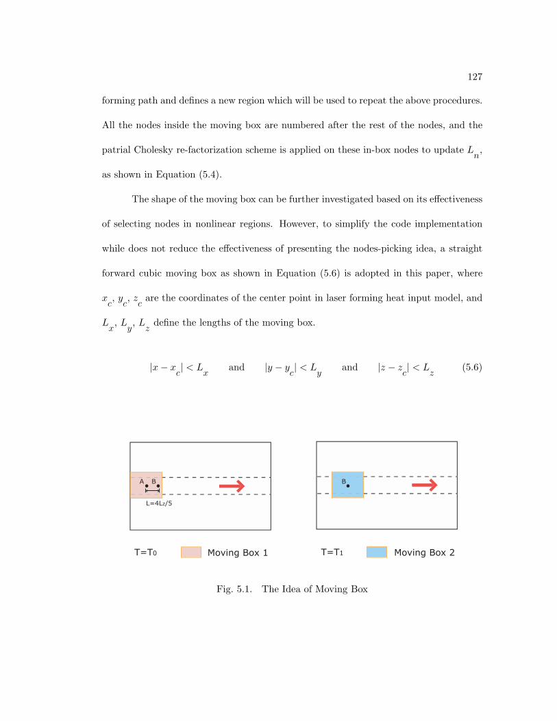
127

forming path and defines a new region which will be used to repeat the above procedures.

All the nodes inside the moving box are numbered after the rest of the nodes, and the

patrial Cholesky re-factorization scheme is applied on these in-box nodes to update Ln,

as shown in Equation (5.4).

The shape of the moving box can be further investigated based on its effectiveness

of selecting nodes in nonlinear regions. However, to simplify the code implementation

while does not reduce the effectiveness of presenting the nodes-picking idea, a straight

forward cubic moving box as shown in Equation (5.6) is adopted in this paper, where

xc, y

c, z

care the coordinates of the center point in laser forming heat input model, and

Lx, L

y, L

zdefine the lengths of the moving box.

|x − xc| < L

xand |y − y

c| < L

yand |z − z

c| < L

z(5.6)

T=T0 Moving Box 1 T=T1 Moving Box 2

A B B

L=4Lz/5

Fig. 5.1. The Idea of Moving Box

128

The idea of moving box is shown in Figure 5.1. Assuming the laser forming is

carried on in the z direction with velocity v, each time the laser beam starts from the

center point of the current moving box (Node A in Figure 5.1) and moves along z direction

for some distance L before it reaches the front boundary of the moving box. After that,

a new moving box with its center defined in the current location of the laser beam (Node

B in Figure 5.1) will be used in the successive time increments. The above procedure

will be repeated until the material processing is finished. Distance L should be less than

Lz

since high temperature results also exist in the region ahead of the laser beam, and

this region should also be covered by the moving box. For the implementations in this

paper, L is chosen to be 4/5Lz

for efficiently utilizing the moving box. Therefore, the

time gap between redefining moving boxes is 4Lz/5v.

5.4.2 Model and Material Properties Simplifications

In modeling industrial scale laser forming applications, if the finite element model

is built based on the standard meshing criteria, very dense mesh is required along the

laser forming path [28, 29]. Therefore, the laser forming introduced nonlinear region,

which is required to be updated from time to time, generally may contain tens of thou-

sands of equations. According to the performance prediction given in Section 5.3, the

effectiveness of the partial Cholesky re-factorization scheme can be verified when the ra-

tio of the updated equation with respect to the total equation is less than 5%. Therefore,

a very large laser forming model is required to be built and simulated to verify this idea.

However, it is not feasible to implement such a large model due to the current computer

resource availability and memory limits. Another computational difficulty is caused by

129

the material nonlinearity and plasticity in low temperature range (below 100 oC), which

also contributes to a larger nonlinear region (with small nonlinearities in most of the

region) and increases the total number of equations to be updated.

With the objective to verify the idea of partial Cholesky re-factorization scheme

under the current computational resource limit, several simplifications are made on model

meshing and its material properties to reduce equations involved in the updated region

and help to define a smaller moving box. They are discussed as follows:

1. Instead of meshing four quadratic elements along each axis for the laser forming

model [28, 29], two elements are used in the simplified model.

2. All the material properties are assumed constants below 100 oC.

3. The yielding stress is set to a very high value (386,100 N/mm2) below 100 oC, so

that no active plasticity exists in regions with temperature lower than 100 oC.

The first simplification reduces equations involved in the updated region. Since

the mesh density is changed, the results from the simplified laser forming model may

be different compared to that from a proper modeled laser forming analysis. However,

from a performance point of view, this does not prevent it from predicting numerical

performance for true scale laser forming models. The second and the third simplifications

modify the material properties and reduce the nonlinearity introduced below 100 oC.

Thus, they reduce the size of the moving boxes. Two independent simulations are tested

with the original material properties and the modified material properties on the medium

size laser forming model in the next section, and the results from the mechanical analysis

show that these two simplifications does not change the stress and distortion results.

130

5.5 Numerical Examples and Performance Results

5.5.1 The Laser Forming Heat Source Model and Material Properties

During the thermal analysis applied to simulate heat propagation and temper-

ature distribution in laser forming, a Gaussian distribution heat input model [11] is

used to represent the laser forming heat flux during the transient thermal analysis. The

formulation is shown in Equation (5.7).

Q =3ηQ

w

πR2

[e−3

(( xR )2+( z

R )2)]

(5.7)

Where Qw

is the laser forming heat input power, η is the laser forming efficiency,

x and z are the local coordinates of a surface point (which is in the XZ plane for the

models in this paper) aligned with the center of the laser beam, R is the radius of the

laser beam, and v is the torch travel speed. For the models simulated in this paper,

these parameters are set as follows: Qw

=1690 W, η=1, R=10 mm, and v=100 mm/s.

The material used in the laser forming simulations is aluminum alloy 2519. The

temperature dependent thermal conductivity K and specific heat Cp

are based on the

Aloca green book, and the density of the alloy is 2.82 × 103 kg/m3. The latent heat

of fusion is set to be 282 kJ/kg/oC and the temperature range of phase transition from

solid to liquid is set from 555 oC to 668 oC. The ambient (room) temperature is set to

be 25 oC.

131

5.5.2 Simulation Software and Hardware

The standard direct sparse solver used in the simulations is DSCPACK, ver-

sion 1.1, which is a package developed with C language by Raghavan [85, 86] to solve

large sparse linear systems using direct methods on multiprocessors and networks-of-

workstations. For this solver, nested dissection ordering scheme is used to order the

system so that fill-ins generated during symbolic factorizations are reduced. The partial

Cholesky re-factorization scheme is implemented in the package DSCPACK-S by Ragha-

van. DSCPACK-S is based on DSCPACK, but with the additional matrix updating/re-

factorization features added.

The in-house finite element analysis code is used to simulate quasi-state thermo-

elasto-plastic processes for laser forming applications. An implicit solution scheme using

the Newton-Raphson method is used to solve nonlinear problems in the iterative fashion.

The code is developed with Fortran 90, and Fortran/C interfaces are added to integrate

the above two DSCPACK solvers.

BLAS is implemented in both DSCPACK packages and the in-house finite element

code to improve the performance of basic vector and matrix related operations. The

implementation currently uses the Intel Math Kernel Library (MKL), version 7.0. The

compilers used are Intel ifort and icc.

The simulation is performed on an Unisys ES7000 system. The system is 16-way

SMP based on 64-bit Intel Itanium2 processors, with 6 MB cache each. Shared memory

is 32 GB and clock is 1.5 GHz per CPU. The OS is RedHat Enterprise 3 Linux. The

132

non-local hard disk access is via NFS. Currently, only serial running performance results

are measured and compared.

5.5.3 Three Simplified Laser Forming Models and Results

Three simplified laser forming plate models are simulated and compared to in-

vestigate the scalability performance of the standard direct sparse solver and the solver

with the partial Cholesky re-factorization scheme. The only difference between these

three models is the plate length: they are 20000 mm for the small size model, 40000 mm

for the medium size model, and 80000 mm for the large size model.

Total DOFs Updated DOFs

Small Model 238833 3525

Medium Model 477333 3525

Large Model 954333 3525

Table 5.1. Models Information

The medium size model is shown in Figure 5.2. This is a plate model with

dimensions: length=40000 mm, width=2000 mm, and thickness=5 mm. The mesh

density along the laser forming path is greatly reduced as specified in section 5.4.2.

A cubic moving box is used to select nodes that are required to be updated. The

dimensions of the moving box are: Lx=200 mm, L

y=200 mm, L

z=500 mm. The box

133

moves and defines a new region for updating every 45 time increments. The total number

of equations for this model is 477333, and the maximum number of updated equations

is 3525. The model information for the small size and the large size model is also shown

in Table 5.1.

The first 100 time increments are simulated. The temperature and stress results

are shown in Figures 5.3 and 5.4. From the temperature results, it can be seen that only

a small region near the heat flux results in temperature higher than 100 oC. Therefore,

with the simplifications introduced in section 5.4.2, nonlinearity is a local phenomenon

and it can be covered by a small moving box.

5.5.4 Performance Results

DSCPACK 1.1 DSCPACK-S

Ordering 10.0 s 17.1 s

Symbolic Factorization 0.4 s 0.6 s

Full Factorization ≈ 25.4 s ≈ 28.8 s

Updated Factorization ≈ 25.4 s ≈ 4.3 s

Solve ≈ 1.0 s ≈ 1.1 s

Peak Memory Usage 2.2 Gb 4.9 Gb

Total Solver CPU for 100 increments 8824.1 s 1923.1 s

Table 5.2. Performance Results for the Small Simplified Laser Forming Model

134

X

Y

ZX

Y

Z

Fig. 5.2. Meshes for the Medium Simplified Laser Forming Model

135

X

Y

Z

3.63+02

3.40+02

3.17+02

2.94+02

2.71+02

2.48+02

2.25+02

2.02+02

1.79+02

1.57+02

1.34+02

1.11+02

8.78+01

6.50+01

4.21+01

1.92+01

X

Y

Z

Fig. 5.3. Thermal Results for the Medium Simplified Laser Forming Model

136

X

Y

Z

2.39+02

2.23+02

2.07+02

1.91+02

1.75+02

1.59+02

1.43+02

1.27+02

1.11+02

9.54+01

7.95+01

6.36+01

4.77+01

3.18+01

1.59+01

1.34-05

X

Y

Z

Fig. 5.4. Stress (Cauchy) Results for the Medium Simplified Laser Forming Model

137






Solve ≈ 2.0 s ≈ 1.6 s



Table 5.3. Performance Results for the Medium Simplified Laser Forming Model

The mechanical analysis performance results for the three models are shown in

Tables 5.2, 5.3 and 5.4. In DSCPACK 1.1, since all the systems are solved in a similar

fashion, there is no difference between full factorizations and updated factorizations.

It is observed that DSCPACK-S takes a bit more time during the stages of or-

dering, symbolic factorization, full factorization and solve. This is reasonable since a

restricted ordering scheme is applied on the system. However, for this scheme, the time

spend on updated factorizations is greatly reduced compared to that in DSCPACK 1.1.

In the three models, it is reduced 5.9, 12.6 and 15.4 times, respectively. The costs per

factorization for all the three models are also shown in Figure 5.5. It is observed that

the costs of DSCPACK 1.1 grows linearly with the size of the problem, which is due to

138






Solve ≈ 3.8 s ≈ 4.6 s



Table 5.4. Performance Results for the Large Simplified Laser Forming Model

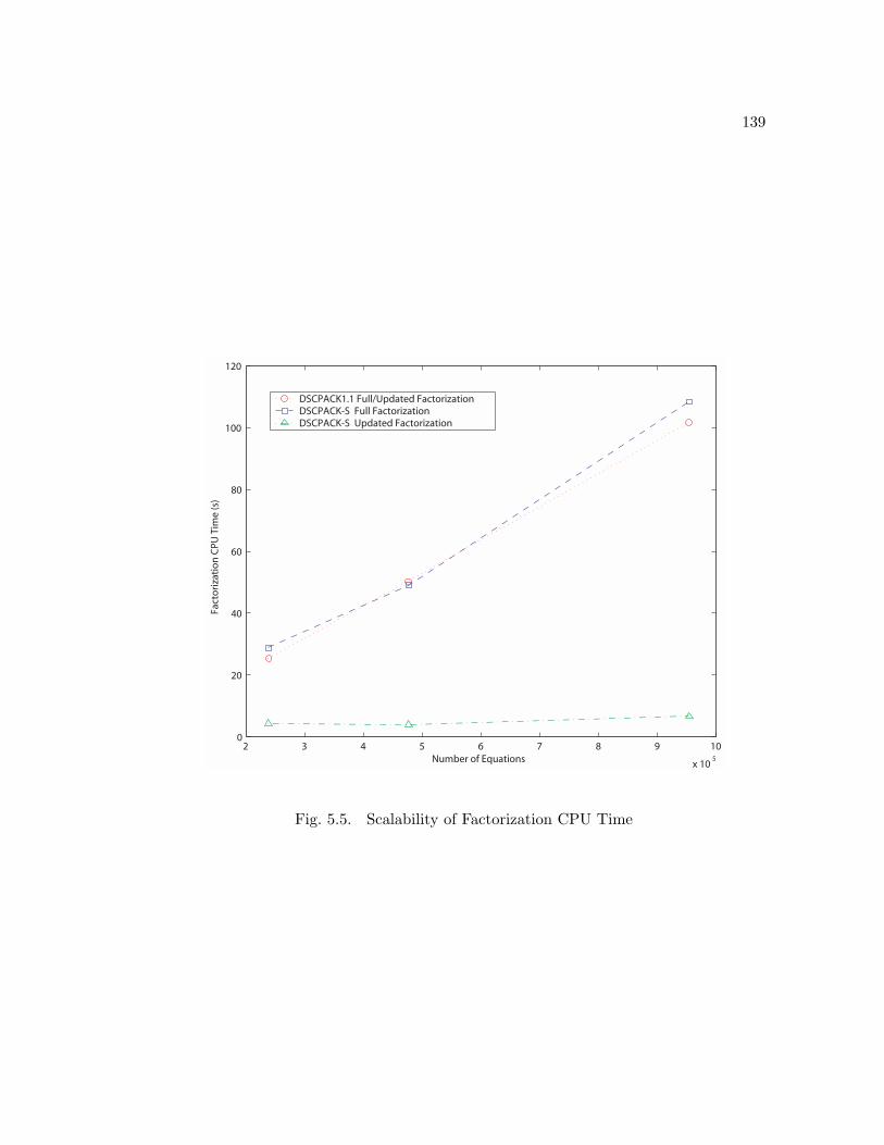
139

2 3 4 5 6 7 8 9 10

x 105

0

20

40

60

80

100

120

Number of Equations

Fact

oriz

atio

n C

PU T

ime

(s)

DSCPACK1.1 Full/Updated FactorizationDSCPACK-S Full FactorizationDSCPACK-S Updated Factorization

Fig. 5.5. Scalability of Factorization CPU Time

140

the fact that the structures tested are long slender plates, and the first separator gener-

ated by the nest dissection ordering scheme only consists a few nodes. The costs of full

factorizations of DSCPACK-S are a little bit higher than DSCPACK 1.1 and also grows

linearly with the size of the problems. The costs of updated factorizations are almost

constant for all the three models, which is due to the fact that the size of the moving

box does not change as the size of the model increases. Finally, the total CPU for the

first 100 increments in three mechanical analyses is reduced by a factor of 4.6, 8.3 and

8.3.


In this paper, the partial Cholesky re-factorization algorithm is implemented and

investigated for large scale applications with localized nonlinearity. This algorithm is

tested on laser forming applications, and its performance is compared to the standard

direct sparse solver DSCPACK 1.1. High speedup is achieved for the testing problems,

and additional improvement can be predicted for even larger applications based on the

computational cost estimations of both approaches. The future work is to extend this

method to other material processing applications and implement parallel/distributed

computing into the algorithm.

141

Chapter 6

Conclusions

As discussed in Chapter 1, 3D large scale finite element material processing sim-

ulations are widely recognized as computationally challenging problems. Large scale

models are required to include more details of the mechanism related to applications,

so that more reliable numerical results can be provided. These models are also essen-

tial to simulate complicated phenomena and processes which is difficult to capture by

a simplified model. However, from a computational point of view, the resulting finite

element equations arising from these large scale applications may easily exceed a million,

which pose many challenges for currently available numerical algorithms and computer

hardware.

This thesis mainly proposes several effective and efficient numerical methods and

computational techniques that can be applied to accelerate 3D large scale finite element

material processing simulations. The application domain investigated in this thesis in-

cludes the welding and laser forming processes.

The first approach, as shown in Chapter 2, introduces parallel computing to the

material processing area and discusses serval related modeling and optimization issues for

simulating welding distortion in large structures. The FEA algorithm is also carefully

implemented on a large shared memory computer and optimized to achieve the most

favorable computational performance. The optimized approach is applied on the large

142

scale Maglev beam problem with 1.27 million equations, and the computational statistics

demonstrate that this approach provides a feasible way to simulate large scale welding

applications in a short amount of time.

The second approach, as shown in Chapter 3, proposes RBS and LNA for the

standard FETI-DP algorithm. RBS is based on the motivation to reduce CPU costs

in many time consuming back-substitutions involved in the PCG iterations. Through a

specific ordering, RBS reduces the equations involved in the back-substitutions, thus it

improves computational speed. LNA is also adopted based on the nature of problems

with localized nonlinearity. It reduces numeric factorizations through a pre-identification

procedure of subdomains, and it also reduces the overhead arising from the specific RBS

ordering scheme. This combined FETI-DP-RBS-LNA approach can reduce CPU costs

effectively for large scale welding applications.

The third approach, as shown in Chapter 4, introduces distributed computing

to this area. The FETI-DP-RBS-LNA algorithm is implemented with two versions of

MPI: MPICH and MPIGM. A 16-subdomain large scale welding problem is tested on

a distributed PC cluster with the standard ethernet interconnect and the high-speed

Myrinet interconnect. The computational performance is evaluated for the first iteration

and a speedup of 8.4 is gained for the MPICH implementation and 14.0 is gained for the

MPIGM implementation.

The fourth approach, as shown in Chapter 5, investigates the partial Cholesky

re-factorization algorithm and its implementation for large scale material processing

applications. This algorithm is tested on three laser forming applications, and its perfor-

mance is compared to the standard direct sparse solver DSCAPCK 1.1. A high speedup

143

of 8.3 is achieved based on the current implementation, and additional improvement can

be predicted for even larger applications based on the computational cost estimations of

both approaches.

The computational costs of the standard direct sparse method, the FETI-DP-

RBS-LNA method and the partial Cholesky re-factorization method for large scale ma-

terial processing problems with localized nonlinearity are estimated in Figure 6.1. The

trends shown in Figure 6.1 indicate that, as the size of the problem grows, the costs

of the standard direct sparse method will grow nonlinearly; the costs of the FETI-

DP-RBS-LNA method will grow almost linearly, and the costs of the partial Cholesky

re-factorization method will not change.

144

2 3 4 5 6 7 8 9 10 11

x 105

0

100

200

300

400

500

600

700

Number of Equations

Solv

er T

ime

(s)

The Standard Direct Sparse MethodThe FETI-DP-RBS-LNA MethodThe Partial Cholesky Re-factorization Method

Fig. 6.1. Estimation of Computational Costs

145

References

[1] R. Gunnert. Residual Welding Stressed. Almqvist & Wiksell, Stockholm, 1955.

[2] K. Terai. Study on Prevention of Welding Deformation in Thin-Skin Plate Struc-

tures. Technical Report 61, Kawasaki, 1978.

[3] Y. Shim, Z. Feng, S. Lee, D.S. Kim, J. Jaeger, J. C. Paparitan, and C. L. Tsai.

Determination of Residual Stress in Thick-Section Weldments. Welding Journal,

71:305s–312s, 1992.

[4] L. P. Connor, editor. Welding Handbook. American Welding Society, Miami, FL,

eighth edition, 1987.

[5] G.H. Jung and C.L. Tsai. Plasticity-based distortion analysis for fillet welded thin-

plate t-joints. Welding Journal, 83(6):177–187, 2004.

[6] P. Michaleris and A. DeBiccari. Prediction of Welding Distortion. Welding Journal,

76(4):172–180, 1997.

[7] K. Masubuchi. Analysis of Welded Structures. Pergamon Press, Oxford, 1980.

[8] H. Hibbitt and P. V. Marcal. A Numerical, Thermo-Mechanical Model for the Weld-

ing and Subsequent Loading of a Fabricated Structure. Computers & Structures,

3(1145-1174):1145–1174, 1973.

146

[9] J. H. Argyris, J. Szimmat, and K. J. Willam. Computational Aspects of Welding

Stress Analysis. Computer Methods in Applied Mechanics and Engineering, 33:635–

666, 1982.

[10] V.J Papazoglou and K. Masubuchi. Numerical Analysis of Thermal Stresses dur-

ing Welding including Phase Transformation Effects. Journal of Pressure Vessel

Technology, 104:198–203, 1982.

[11] J. Goldak, A. Chakravarti, and M. Bibby. A New Finite Element Model for Welding

Heat Sources. Metallurgical Transactions B, 15B:299–305, 1984.

[12] J.B. Leblond and J. Devaux. A New Kinetic Model for Anisothermal Metallurgical

Transformations in Steels Including Effect of Austenite Grain Size. Acta Mettal,

32(1):137–146, 1984.

[13] D.F. Watt, L. Coon, M.J. Bibby, J. Goldak, and C. Henwwod. An Algorithm for

modeling Microstructural Development in weld heat-affected zones. Acta Metall,

36(11):3029–3035, 1988.

[14] C. Henwood, M. Bibby, J. Goldak, and D. Watt. Coupled Transient Heat Transfer-

Microstructure Weld Computations, Part B. Acta Metall, 36(11):3037–3046, 1988.

[15] A. S. Oddy, J. A. Goldak, and J. M. J. McDill. Numerical Analysis of Transfor-

mation Plasticity in 3 D Finite Element Analysis of Welds. European Journal of

Mechanics, A/Solids, 9(3):253–263, 1990.

147

[16] P. Tekriwal and J. Mazumder. Transient and Residual Thermal Strain-Stress Anal-

ysis of GMAW. Journal of Engineering Materials and Technology, 113:336–343,

1991.

[17] S.B. Brown and H. Song. Implications of Three-Dimensional Numerical Simulations

of Welding of Large Structures. Welding Journal, 71(2):55s–62s, 1992.

[18] S. Paul, P. Michaleris, and J.Shanghvi. Optimization of Thermo-Elasto-Plastic

Finite Element Analysis using an Eulerian Formulation. International Journal for

Numerical Methods in Engineering, 56:1125–1150, 2003.

[19] J. Shanghvi and J. Dydo. A Transient Thermal Tensioning Process for Midigating

Distortion in Stiffened Structures. In 39th Annual Technical Meeting Society of

Engineering Science, State College, PA, 2002. SES.

[20] J. Goldak and M. Bibby. Computational Thermal Analysis of Welds: Current Status

and Future Directions. In A. F. Giamei and G. J. Abbaschian, editors, Modeling

of Casting and Weldin Processes IV, pages 153–166, Palm Coast, FL, 1988. The

Minerals & Materials Society.

[21] H. J. Braudel, M. Abouaf, and J. L. Chenot. An Implicit and Incremental Formu-

lation for the Solution of Elastoplastic Problems by the Finite Element Method.

Computers and Structures, 22(5):801–814, 1986.

[22] J. M. J. McDill A. S. Oddy and J. A.Goldak. Consistent strain fields in 3d finite

element analysis of welds. ASME Journal of Pressure Vessel Technology, 112(3):309–

311, 1990.

148

[23] L. A. Bertram and A. R Ortega. Automated Thermomechanical Modeling of Welds

Using Interface Elements for 3D Metal Deposition. In Manuscript for Proceedings

of ABAQUS User’s Conference, Oxford: Hibbit Karlsson and Sorensen Inc., 1991.

[24] J. Wang and H. Murakawa. A 3-d fem analysis of buckling distortion during welding

in thin plate. In 5th International Conference in Trends in Welding Research, Pine

Mountain, GA, 1998.

[25] J. B. Roelens and F. Maltrud. Determination of residual stresses in submerged arc

multi-pass welds by means of numerical simulation and comparison with experimen-

tal measurements. In IIW Annual Assembly, Glasgow, 1993. Doc. X-1279.

[26] E. F. Rybicki and R. B. Stonesifer. Computation of Residual Stresses due to Multi-

pass Welds in Piping Systems. Journal of Pressure Vessel Technology, 101:149–154,

1979.

[27] A. P. Chakravati, L. M. Malik, and J. A. Goldak. Prediction of Distortion and

Residual Stresses in Panel Welds. In Computer modelling of fabrication processess

and constitutive behaviour of metals, pages 547–561, Ottawa, Ontario, 1986.

[28] J. Goldak, M. Bibby, J. Moore, R. House, and B. Patel. Computer Modeling of

Heat Flows in Welds. Metallurgical Transactions B, 17B:587–600, 1986.

[29] L. Zhang, E.W. Reutzel, and P. Michaleris. Finite Element Modeling Discretization

Requirements for the Laser Forming Process. International Journal of Mechanical

Sciences, 46:623–637, 2004.

149

[30] J. C. Simo and R. L. Taylor. Consistent Tangent Operators for Rate-Independent

Elasto-Plasticity. Computer Methods in Applied Mechanics and Engineering,

48:101–118, 1985.

[31] P. Michaleris, D. A. Tortorelli, and C. A. Vidal. Analysis and Optimization of

Weakly Coupled Thermo-Elasto-Plastic Systems with Applications to Weldment

Design. International Journal for Numerical Methods in Engineering, 38(8):1259–

1285, 1995.

[32] N.S. Prasad and T. K. Sankaranrayanan. Estimation of residual stresses in weld-

ments using adaptive grids. Computers and Structures, 60(6):1037–1045, 1996.

[33] H. Runnemalm and S. Hyun. Three-dimensional welding analysis using an adaptive

mesh scheme. Computer Methods in Applied Mechanics and Engineering, 189:515–

523, 2000.

[34] C. Farhat, M. Lesoinne, and K. Pierson. A scalable dual-primal domain decompo-

sition method. Numerical Linear Algebra with Applications, 7:687–714, 2000.

[35] C. Farhat, M. Lesoinne, P. LeTallec, K. Pierson, and D. Rixen. FETI-DP: a dual-

primal unified FETI method - part I: A faster alternative to the two-level FETI

method. International Journal for Numerical Methods in Engineering, 50:1523–

1544, 2001.

[36] Anshul Gupta, George Karypis, and Vipin Kumar. Highly scalable parallel algo-

rithms for sparse matrix factorization. IEEE Transactions on Parallel and Dis-

tributed Systems, 8(5):502–520, May 1997.

150

[37] Anshul Gupta. WSMP: Watson sparse matrix package (Part-I: direct solu-

tion of symmetric sparse systems). Technical Report RC 21886 (98462), IBM

T. J. Watson Research Center, Yorktown Heights, NY, November 16, 2000.

http://www.cs.umn.edu/˜agupta/wsmp.

[38] K. J. Bathe. Finite Element Procedures. Prentice-Hall, Inc., New Jersey, NJ, 1996.

[39] The British Iron and Steel Research Association, editor. Physical Constants of Some

Commercial Steels at Elevated Temperatures. Butterworths Scientific Publications,

London, 1953.

[40] L. O. Raymond and J. Chipman. Thermodynamic Functions of Iron. Transactions

of the Metallurgical Society of AIME, 239:630–633, 1967.

[41] L.-E. Lindgren. Finite element modelling and simulation of welding, Part 2 Improved

material modelling. Journal of Thermal Stresses, 24:195–231, 2001.

[42] Maglev Inc. Web page content. http://www.maglevpa.com, 2004.

[43] R. J. Lipton, D. J. Rose, and R. E. Tarjan. Generalized nested dissection. SIAM

journal on numerical analysis, 16:346–358, 1979.

[44] G. Kron. A set of principles to interconnect the solutions of physical systems.

Journal of Applied Physics, 24(8):965–980, 1953.

[45] W. Przemieniecki. Matrix structural analysis of substructures. American Institute

of Aeronautics and Astronautics Journal, 1:138–147, 1963.

151

[46] C. Farhat and E. Wilson. A new finite element concurrent computer program archi-

tecture. International Journal for Numerical Methods in Engineering, 24(9):1771–

1792, 1987.

[47] J. Mandel. Balancing domain decomposition. Communications In Applied Numer-

ical Methods, 9:233–241, 1993.

[48] C. Farhat and F.X. Roux. A method of finite element tearing and interconnecting

and its parallel solution algorithm. International Journal for Numerical Methods in

Engineering, 32:1205–1227, 1991.

[49] C. Farhat and J. Mandel. The two-level FETI method for static and dynamic plate

problems Part I: An optimal iterative solver for biharmonic systems. Computer

Methods in Applied Mechanics and Engineering, 155:129–152, 1998.

[50] C. Farhat. A Lagrange multiplier based divide and conquer finite element algorithm.

Journal of Computer and Systems Engineering, 2:149–156, 1991.

[51] C. Farhat. A Saddle-Point Principle Domain Decomposition Method for the Solu-

tion of Solid Mechanics Problems. In D. E. Keyes, T. F. Chan, G. A. Meurant,

J. S. Scroggs, and R. G. Voigt, editors, Domain Decomposition Methods for Partial

Differential Equations, pages 271–292. SIAM, 1992.

[52] C. Farhat and F.X. Roux. Implicit parallel processing in structural mechanics.

Computational Mechanics Advances, 2(1):1–124, 1994.

152

[53] C. Farhat and F. X. Roux. An unconventional domain decomposition method for

an efficient parallel solution of large-scale finite element systems. SIAM Journal on

Scientific and Statistical Computing, 13(1):379–396, 1992.

[54] C. Farhat, J. Mandel, and F. X. Roux. Optimal convergence properties of the

FETI domain decomposition method. Computer Methods in Applied Mechanics

and Engineering, 115:367–388, 1994.

[55] J. Mandel and R. Tezaur. Convergence of a substructuring method with Lagrange

multipliers. Numerische Mathematik, 73:473–487, 1996.

[56] R. Tezaur. Analysis of Lagrange multiplier based domain decomposition. Phd thesis,

University of Colorado at Denver, 1998.

[57] M. Bhardwaj, D. Day, C. Farhat, M. Lesoinne, K. Pierson, and D. Rixen. Appli-

cation of the FETI method to ASCI problems: scalability results on one-thousand

processors and discussion of highly heterogeneous problems. International Journal

for Numerical Methods in Engineering, 47:513–536, 2000.

[58] C. Farhat, P.S. Chen, J. Mandel, and F.X. Roux. The two-level FETI method Part

II: Extension to shell problems, parallel implementation and performance results.

Computer Methods in Applied Mechanics and Engineering, 155:153–180, 1998.

[59] C. Farhat, P.S. Chen, F. Risler, and F.X. Roux. A unified framework for accelerat-

ing the convergence of iterative substructuring methods with Lagrange multipliers.

International Journal for Numerical Methods in Engineering, 42:257–288, 1998.

153

[60] J. Mandel, R. Tezaur, and C. Farhat. A scalable substructuring method by La-

grange multipliers for plate bending problems. SIAM Journal on Numerical Anal-

ysis, 36:1370–1391, 1999.

[61] C. Farhat and M. Geradin. On a component mode synthesis method and its ap-

plication to incompatible substructures. Computers and Structures, 51:459–473,

1994.

[62] C. Farhat, P. S. Chen, and J. Mandel. A scalable lagrange multiplier based domain

decomposition method for implicit time-dependent problems. International Journal

for Numerical Methods in Engineering, 38:3831–3845, 1995.

[63] C. Farhat, C. Lacour, and D. Rixen. Incorporation of linear multipoint constraints

in substructure based iterative solvers - Part I: A numerically scalable algorithm.

International Journal for Numerical Methods in Engineering, 43:997–1016, 1998.

[64] Patrick Le Tallec and Marina Vidrascu. Efficient solution of mechanical and biome-

chanical problems by domain decomposition. Numerical linear algebra with appli-

cations, 6(7):599–616, 1999.

[65] C. Farhat, A. Macedo, and M. Lesoinne. A two-level domain decomposition method

for the iterative solution of high frequency exterior Helmholtz problems. Numerische

Mathematik, 85:283–308, 2000.

[66] C. Farhat, K. Pierson, and M. Lesoinne. The second generation of FETI methods

and their application to the parallel solution of large-scale linear and geometrically

154

nonlinear structural analysis problems. Computer Methods in Applied Mechanics

and Engineering, 184:333–374, 2000.

[67] A. Toselli. FETI domain decomposition methods for scalar advection-diffusion prob-

lems. Computer Methods in Applied Mechanics and Engineering, 190:5759–5776,

2001.

[68] D. Dureisseix and C. Farhat. A numerically scalable domain decomposition method

for the solution of frictionless contact problems. International Journal for Numerical

Methods in Engineering, 50:2643–2666, 2001.

[69] B. Vereecke, H. Bavestrello, and D. Dureisseix. An extension of the FETI domain

decomposition method for incompressible and nearly incompressible problems. Com-

puter Methods in Applied Mechanics and Engineering, 192:3409–3429, 2003.

[70] R. Kanapady and K. K. Tamma. A-scalability of an integrated computational

technology and framework for non-linear structural dynamics - Part I: Theoreti-

cal developments and parallel formulations. International Journal for Numerical


[71] R. Kanapady and K. K. Tamma. A-scalability of an integrated computational tech-

nology and framework for non-linear structural dynamics - Part II: Implementation

aspects and parallel performance results. International Journal for Numerical Meth-

ods in Engineering, 58:2295–2323, 2003.

155

[72] C. Farhat, L. Crivelli, and F. X. Roux. Extending substructure based iterative

solvers to multiple load and repeated analyses. Computer Methods in Applied Me-

chanics and Engineering, 117:195–209, 1994.

[73] C. Farhat and P. S. Chen. Tailoring domain decomposition methods for efficient par-

allel coarse grid solution and for systems with many right hand sides. Contemporary

Mathematics, 180:401–406, 1994.

[74] M. Papadrakakis and Y. Tsompanakis. Domain decomposition methods for parallel

solution of shape sensitivity anlysis problems. International Journal for Numerical


[75] D. Rixen and C. Farhat. A simple and efficient extension of a class of substructure

based preconditioners to heterogeneous structural mechanics problems. Interna-

tional Journal for Numerical Methods in Engineering, 44:489–516, 1999.

[76] David Kincaid and Ward Cheney. Numerical Analysis: Mathematics of Scientific

Computing. Brooks/Cole/Thomson Learning, Pacific Grove, CA, 3rd edition, 2002.

[77] A. George, J. Liu, and E. Ng. Computer Solutions of Sparse Positive Definite

Systems. course material, to be published.

[78] D. J. Rose, R. E. Tarjan, and G. S. Lueker. Algorithmic aspects of vertex elimination

on graphs. SIAM Journal on Computing, 5:266–283, 1976.

[79] J. Sun, P. Michaleris, A. Gupta, and P. Raghavan. A Fast Implementation of the

FETI-DP Method: FETI-DP-RBS-LNA and Applications on Large Scale Problems

156

with Localized Nonlinearitie. International Journal for Numerical Methods in En-

gineering, 63(6):833–858, 2005.

[80] P. Raghavan, M. A. James, J. C. Newman, and B. R. Seshadri. Scalable sparse

matrix techniques for modeling crack growth. In Lecture Notes in Computer Sci-

ence, Proceedings of PARA’02, Applied Parallel Computing, pages 588–602, Espoo,

Finland, June 2002.

[81] P. E. Gill, G.H. Golub, W. Murray, and M. A. Saunders. Methods for modifying

matrix factorizations. Mathematics of Computation, 28:505–535, 1974.

[82] T. A. Davis and W. W. Hager. Modifying a sparse cholesky factorization. SIAM

Journal on Matrix Analysis and Applications, 20:606–627, 1999.

[83] Timothy A. Davis and William W. Hager. Multiple-rank modifications of a

sparse Cholesky factorization. SIAM Journal on Matrix Analysis and Applications,

22(4):997–1013, 2001.

[84] W. W. Hager. Updating the inverse of a matrix. SIAM Rev., 31(2):221–239, 1989.

[85] P. Raghavan. DSCPACK home page. http://www.cse.psu.edu/ ragha-

van/software.html, 2001.

[86] P. Raghavan. DSCPACK: Domain-Separator Codes for the parallel solution of

sparse linear systems. Tech. rep. cse-02-004, Department of Computer Science and

Engineering, The Pennsylvania State University, University Park, PA 16802-6106,

2002.

Vita

Jun Sun received his BE degree in Structural Mechanics from the Department of

Mechanics and Engineering Science at Beijing University in June 2000. In Aug 2000, he

enrolled in the graduate program in Mechanical Engineering at the Pennsylvania State

University and began to pursue his PhD degree. He is also studying for a concurrent MS

degree in the Department of Computer Science and Engineering. His research interests

include solid mechanics, thermal processing, nonlinear finite element analysis, numeric

methods, and high performance parallel and distributed computing.

modeling and finite element analysis of welding

Documents