sensors

Article

Modeling and Calibration of a Novel One-MirrorGalvanometric Laser ScannerChengyi Yu 1, Xiaobo Chen 1 and Juntong Xi 1,2,*

1 State Key Laboratory of Mechanical System and Vibration, Shanghai Jiaotong University, Shanghai 200240,China; jg5bvictor@sjtu.edu.cn (C.Y.); xiaoboc@sjtu.edu.cn (X.C.)

2 Shanghai Key Laboratory of Advanced Manufacturing Environment, Shanghai 200030, China* Correspondence: jtxi@sjtu.edu.cn; Tel.: +86-21-3420-5693

Academic Editor: Thierry BoschReceived: 19 October 2016; Accepted: 12 January 2017; Published: 15 January 2017

Abstract: A laser stripe sensor has limited application when a point cloud of geometric sampleson the surface of the object needs to be collected, so a galvanometric laser scanner is designedby using a one-mirror galvanometer element as its mechanical device to drive the laser stripe tosweep along the object. A novel mathematical model is derived for the proposed galvanometerlaser scanner without any position assumptions and then a model-driven calibration procedureis proposed. Compared with available model-driven approaches, the influence of machining andassembly errors is considered in the proposed model. Meanwhile, a plane-constraint-based approachis proposed to extract a large number of calibration points effectively and accurately to calibratethe galvanometric laser scanner. Repeatability and accuracy of the galvanometric laser scanner areevaluated on the automobile production line to verify the efficiency and accuracy of the proposedcalibration method. Experimental results show that the proposed calibration approach yields similarmeasurement performance compared with a look-up table calibration method.

Keywords: galvanometric laser scanner; calibration; the screw theory; laser stripe sensor

1. Introduction

In recent decades, the laser stripe sensor has been widely used and is becoming promising inmany industrial applications, such as a seam tracking system [1], a weld quality inspecting system [2]and an inspection system of automobile assembly [3], because of its fast acquisition speed, very simplemechanical structure, low cost, and robustness. The main working principle of the laser stripe sensoris that a laser line projector projects a single laser stripe plane onto the object’s surface, forming a lightstripe. The light stripe is modulated by the depth of the object’s surface and a camera records the 2Ddistorted image. The 3D characteristic information of the object’s surface can be derived from the2D distorted image after performing 3D reconstruction. However, a laser stripe sensor has limitedapplication when a point cloud of geometric samples on the surface of the object is needed to becollected [4]. Taking an inspection system of automobile assembly, for example, the alignments ofholes and parts are important, because imprecise positioning of screw holes on a body frame can twistthe frame, loosen screws, produce vibration, and deteriorate other qualities. Consequently, the lightstripe needs to sweep through the surface of the hole by using mechanical devices to extract its center.The system with such a scanning capability is called a laser scanner.

Tremendous efforts have been devoted to the field of developing and calibrating many laserscanners with different mechanical devices and a wide range of methods have been developed. Li [5–7]designed a laser scanner via mounting the laser stripe sensor to the end-effect of a robot. The accuracyof the laser scanner is limited owing to the absolute accuracy of the robot. The laser stripe sensor canalso be fixed at the end of the coordinate measuring machine to form a highly accurate laser scanner [8];

Sensors 2017, 17, 164; doi:10.3390/s17010164 www.mdpi.com/journal/sensors

Sensors 2017, 17, 164 2 of 14

however, the coordinate measuring machine is not suitable for being installed on the productionline. There is also another form of laser scanner where the position of the projector with respect tothe camera coordinate system can be determined via additional reference frame [9,10] or physicalconstraint [11,12]. Ren [13,14] proposed a linear laser scanner via mounting the laser stripe sensor to alinear rail and the linear rail takes the vision sensor to perform linear scanning. The shortcoming ofthe linear laser scanner is that its relatively large size and heavy load of the linear rail will limit itsindustrial applications. Li [15] and Xiao [16] presented a rotational laser scanner by mounting the laserstripe sensor to a turntable. This has the same drawbacks as the linear laser scanner.

The laser scanner using the galvanometric element as its mechanical devices can solve theaforementioned drawbacks. The galvanometric element mainly consists of a precision motor and areflective mirror. The precision motor guarantees the accuracy of the galvanometric laser scanner.Additionally, the load of the precision motor is just the lightweight mirror and it is much lighter thanthe aforementioned laser scanners [13–16]. Furthermore, the galvanometric element is mounted insidethe laser scanner, so the size of the galvanometric laser scanner is relatively smaller. However, existingmethods [17–21] are only deal with the vision sensor calibration problem with a fixed light stripeplane. Additionally, calibration of a linear laser scanner [13,14] or a rotational laser scanner [15,16] isto determine the movement of the vision sensor, and movement of the whole vision sensor is easilyestimated via measuring a static sphere [13,14] or a planar calibration target [15] using the visionsensor. All of the aforementioned calibration methods cannot be used to calibrate the galvanometriclaser scanner. Manakov [22] designed a two-mirror galvanometric laser scanner with a point-marklaser projector and proposed a model-driven calibration method. However, the rotational axis that layson the reflective mirror is assumed in the mathematical model and initial estimations of the intrinsicand extrinsic parameters of the scanning system are calibrated separately. Wagner [23] proposed alook-up table (LUT) to calibrate the two-mirror galvanometric laser scanner and only the pre-definedset of laser rays in LUT can be used in the measuring process. Wissel [24] presented a data-drivenlearning method for calibrating the two-mirror galvanometric laser scanner, however, a large amountof data is needed to train the data-driven model. The point-mark laser projector along with thetwo-mirror galvanometric element spends a lot of time to sweeping through the surface of the object,and consequently, the two-mirror galvanometric laser scanner is not suitable for measuring the shapeof the object on the production line. Recently, Chi [25] proposed a laser line auto-scanning systemfor underwater 3D reconstruction, and it overcomes the time-consuming drawback of the point-marklaser scanner [22]. However, the mathematical model [25] assumes that the galvanometer rotationaxis should completely coincide with the line intersected by the laser plane and the mirror of thegalvanometer. The assumption is relatively harsh for machining and assembly accuracy, becausethe direction of the laser stripe plane is very hard to measure, and consequently, it is impossible toadjust the incoming laser stripe plane to hit the galvanometer rotation axis. In summary, availablemathematical models [22,25] of the galvanometric laser scanner make some assumptions which requirethe system to be manufactured and assembled well enough, so that the available mathematical modelsare limited in actual applications.

In this paper, a novel laser scanner is designed via using a one-mirror galvanometer element asthe mechanical device. Then the corresponding mathematical model and calibration procedure forthe galvanometric laser scanner are proposed. Compared with the linear laser scanner [13,14] andthe rotational laser scanner [15,16], the advantage of the proposed galvanometric laser scanner is thatits size is very small and its light load increases the life of the motor, so the proposed laser scannerhas widespread application prospects in the industrial field, especially for on-line quality inspection.Compared with the mathematical model and the calibration procedure proposed by Manakov [22]and Chi [25], the proposed mathematical model is derived without any position assumptions and allparameters are estimated by minimizing one objective function. The remaining sections are organizedas follows: Section 2 introduces the construction and inspecting principle of the galvanometric laserscanner; in Section 3, the mathematical model of the proposed laser scanner is established. Based on the

Sensors 2017, 17, 164 3 of 14

proposed mathematical model, a calibration procedure for the laser scanner is presented. To validatethe efficiency and accuracy of the proposed method, contrast experiments are conducted in Section 4;and the paper ends with concluding remarks in Section 5.

2. System Working Principles

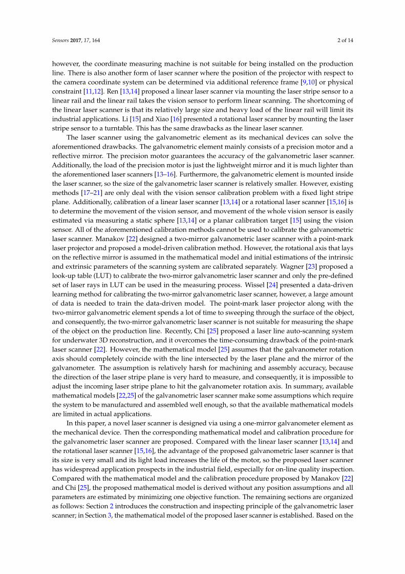
The galvanometric laser scanner is designed using a one-mirror galvanometer element as themechanical device to collect a point cloud of geometric samples on the surface of the object as shownin Figure 1a. As shown in Figure 1b, the galvanometric laser scanner is mainly comprised of a CCDcamera (Basler acA1300/30 µm) with a 16 mm lens, a laser line projector (wavelength of 730 nm,beam width ≤1 mm), and a one-mirror galvanometer element which was made by ourselves using areflective mirror and a stepper motor. The size of the galvanometric laser scanner is 158 × 116 × 43 mm.Here, there are 23 stripe lines in the view of the sensor, and each pose of the stripe line is fixed in theCCS owing to the high repeatability of the stepper motor. Each rotational step of the galvanometerelement is 0.1146◦, which is decided by both the speed of the galvanometer element and the frame rateof the camera.

Sensors 2017, 17, 164 3 of 14

is presented. To validate the efficiency and accuracy of the proposed method, contrast experiments

are conducted in Section 4; and the paper ends with concluding remarks in Section 5.

2. System Working Principles

The galvanometric laser scanner is designed using a one-mirror galvanometer element as the

mechanical device to collect a point cloud of geometric samples on the surface of the object as

shown in Figure 1a. As shown in Figure 1b, the galvanometric laser scanner is mainly comprised

of a CCD camera (Basler acA1300/30 µm) with a 16 mm lens, a laser line projector (wavelength of

730 nm, beam width ≤1 mm), and a one-mirror galvanometer element which was made by

ourselves using a reflective mirror and a stepper motor. The size of the galvanometric laser scanner

is 158 × 116 × 43 mm. Here, there are 23 stripe lines in the view of the sensor, and each pose of the

stripe line is fixed in the CCS owing to the high repeatability of the stepper motor. Each rotational

step of the galvanometer element is 0.1146°, which is decided by both the speed of the galvanometer

element and the frame rate of the camera.

CX

CY

CZ

Camera

Projector

galvanometer

element

mirrorLaser stripe plane

Object

Work Piece

Laser Projector

galvanometer element

Sen

sor

Camera

Z

Y

(a) (b)

Figure 1. (a) Schematic diagram of the one-mirror galvanometric laser scanner; and (b) construction

of the one-mirror galvanometric laser scanner.

The working principle is as follows: an incoming laser stripe plane, which is projected by a laser

line projector, hits the reflective mirror and the light stripe formed by intersecting outgoing laser

stripe plane and the object’s surface is captured by the fixed camera. The 3D characteristic

information of the object’s surface can be derived from the 2D distorted structured light stripe images

after 3D reconstruction. The camera is triggered to acquire pictures continuously when the stepper

motor gives a hardware trigger signal. The hardware trigger signal is given when the stepper motor

rotates across its zero position. The reflected laser stripe plane scans across the object’s surface along

with the rotation of the galvanometer element, and the 3D information of the object’s whole surface

can be reconstructed. The measurement result is obtained within one second along with the scanning,

so it is very suitable for industrial applications, especially for on-line quality inspection. The

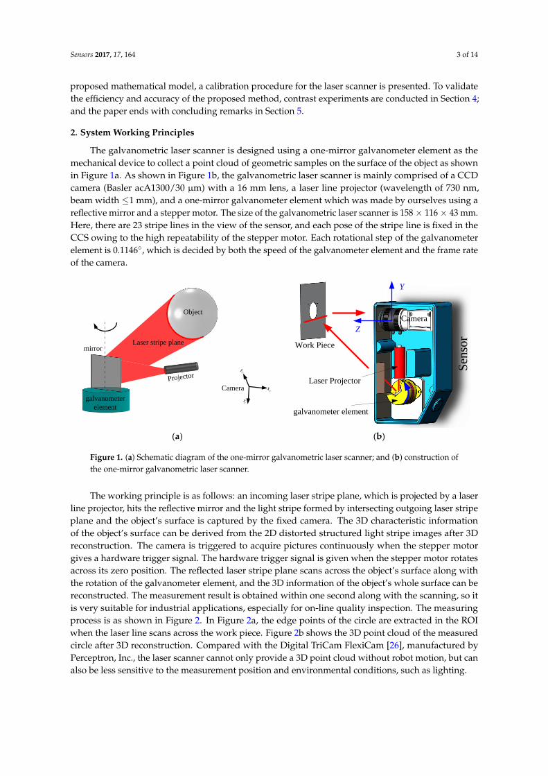
measuring process is as shown in Figure 2. In Figure 2a, the edge points of the circle are extracted in

the ROI when the laser line scans across the work piece. Figure 2b shows the 3D point cloud of the

measured circle after 3D reconstruction. Compared with the Digital TriCam FlexiCam [26],

manufactured by Perceptron, Inc., the laser scanner cannot only provide a 3D point cloud without

robot motion, but can also be less sensitive to the measurement position and environmental

conditions, such as lighting.

Figure 1. (a) Schematic diagram of the one-mirror galvanometric laser scanner; and (b) construction ofthe one-mirror galvanometric laser scanner.

The working principle is as follows: an incoming laser stripe plane, which is projected by a laserline projector, hits the reflective mirror and the light stripe formed by intersecting outgoing laser stripeplane and the object’s surface is captured by the fixed camera. The 3D characteristic informationof the object’s surface can be derived from the 2D distorted structured light stripe images after 3Dreconstruction. The camera is triggered to acquire pictures continuously when the stepper motorgives a hardware trigger signal. The hardware trigger signal is given when the stepper motor rotatesacross its zero position. The reflected laser stripe plane scans across the object’s surface along withthe rotation of the galvanometer element, and the 3D information of the object’s whole surface can bereconstructed. The measurement result is obtained within one second along with the scanning, so itis very suitable for industrial applications, especially for on-line quality inspection. The measuringprocess is as shown in Figure 2. In Figure 2a, the edge points of the circle are extracted in the ROIwhen the laser line scans across the work piece. Figure 2b shows the 3D point cloud of the measuredcircle after 3D reconstruction. Compared with the Digital TriCam FlexiCam [26], manufactured byPerceptron, Inc., the laser scanner cannot only provide a 3D point cloud without robot motion, but canalso be less sensitive to the measurement position and environmental conditions, such as lighting.

Sensors 2017, 17, 164 4 of 14Sensors 2017, 17, 164 4 of 14

Laser Line ROI

Edge points

(a) (b)

Figure 2. The measuring process of the work piece feature: (a) the processed gray image; and (b) the

corresponding 3D point cloud.

3. Modeling and Calibration of the Galvanometric Laser Scanner

The proposed galvanometric laser scanner is calibrated via calibrating the camera first and then

estimating the equation of each laser stripe plane with respect to the camera coordinate system (CCS).

The camera has been extensively studied in the past decades, and its modeling and calibration

techniques are very mature [27–29]. The main obstacle is to determine the equation of the reflected

laser stripe plane with respect to the CCS at a given rotational angle of the galvanometer element. A

mathematic model between the reflected laser plane and the given rotational angle is derived mainly

based on the screw theory, and the objective function is established to identify the unknown

parameters via minimizing the sum of distances from calibration points (control points) on the laser

stripe plane to estimated reflected laser planes. A large number of control points are extracted by

employing a plane-constraint-based method.

3.1. Camera Calibration

Camera calibration is to estimate intrinsic parameters which reflect the optical characteristic of

the camera, and extrinsic parameters that express the pose of the local world coordinate system

relative to the camera coordinate system. Zhang [29] presents a flexible camera calibration algorithm

in which a planar calibration target is observed by a camera from multiple points of view. Here, the

camera is fixed and the 7 × 7 dot array calibration target is freely moved and the relative calibration

target poses are unknown. After camera calibration, the pose of each calibration target with respect

to the camera coordinate system is determined.

3.2. Computing Control Points via the Plane-Constraint-Based Method

Here, a plane-constraint-based approach is proposed to extract a large number of control points

on the laser stripe plane to identify the system’s unknown parameters by viewing a planar calibration

target from multiple orientations. Compared with the invariance of cross-ratio [19,21] and the

invariance of double cross-ratio [20,30], the plane-constraint-based calibration approach extracts the

same number of control points as the invariance of double cross-ratio without error propagation.

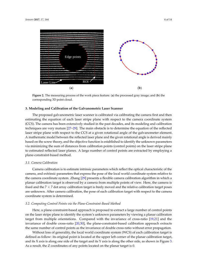
Without loss of generality, the local world coordinate system (WCS) of each calibration target is

defined as follow: its original point is located at the upper left corner of the planar calibration target,

and its X axis is along one side of the target and its Y axis is along the other side, as shown in Figure 3.

As a result, the Z coordinates of any points located on the planar target is 0.

0Z (1)

Figure 2. The measuring process of the work piece feature: (a) the processed gray image; and (b) thecorresponding 3D point cloud.

3. Modeling and Calibration of the Galvanometric Laser Scanner

The proposed galvanometric laser scanner is calibrated via calibrating the camera first and thenestimating the equation of each laser stripe plane with respect to the camera coordinate system(CCS). The camera has been extensively studied in the past decades, and its modeling and calibrationtechniques are very mature [27–29]. The main obstacle is to determine the equation of the reflectedlaser stripe plane with respect to the CCS at a given rotational angle of the galvanometer element.A mathematic model between the reflected laser plane and the given rotational angle is derived mainlybased on the screw theory, and the objective function is established to identify the unknown parametersvia minimizing the sum of distances from calibration points (control points) on the laser stripe planeto estimated reflected laser planes. A large number of control points are extracted by employing aplane-constraint-based method.

3.1. Camera Calibration

Camera calibration is to estimate intrinsic parameters which reflect the optical characteristic of thecamera, and extrinsic parameters that express the pose of the local world coordinate system relative tothe camera coordinate system. Zhang [29] presents a flexible camera calibration algorithm in which aplanar calibration target is observed by a camera from multiple points of view. Here, the camera isfixed and the 7 × 7 dot array calibration target is freely moved and the relative calibration target posesare unknown. After camera calibration, the pose of each calibration target with respect to the cameracoordinate system is determined.

3.2. Computing Control Points via the Plane-Constraint-Based Method

Here, a plane-constraint-based approach is proposed to extract a large number of control pointson the laser stripe plane to identify the system’s unknown parameters by viewing a planar calibrationtarget from multiple orientations. Compared with the invariance of cross-ratio [19,21] and theinvariance of double cross-ratio [20,30], the plane-constraint-based calibration approach extractsthe same number of control points as the invariance of double cross-ratio without error propagation.

Without loss of generality, the local world coordinate system (WCS) of each calibration target isdefined as follow: its original point is located at the upper left corner of the planar calibration target,and its X axis is along one side of the target and its Y axis is along the other side, as shown in Figure 3.As a result, the Z coordinates of any points located on the planar target is 0.

Sensors 2017, 17, 164 5 of 14

Z = 0 (1)

The camera model can be expanded as:

µPi =ci

TCCTw Pw =

t11 t12 t13 t14

t21 t22 t23 t24

t31 t32 t33 t34

Pw (2)

where ciTC and CTw contain intrinsic and extrinsic parameters separately, so they are known after

camera calibration. Pi is the image plane coordinate of a control point which can be determined bycenter of mass algorithm [31] and Pω is the corresponding world coordinates of the control point.

However, ciTC·CTw is a 3 × 4 transformation matrix with row rank r = 3, so there is no left inverse

matrix of ciTC·CTw. As a result, the world control point Pω cannot be derived only from Equation (2).

However, all the world control points are constrained on the surface of the planar target, so there is anadditional equation (Z = 0) for all the world control points. Equations (1) and (2) are combined to formthe plane-constraint-based method for extracting control points in the local WCS:

µ

[Pi0

]= TPw =

t11 t12 t13 t14

t21 t22 t23 t24

t31 t32 t33 t34

0 0 1 0

Pw (3)

where the transformation matrix T is a 4 × 4 invertible matrix, and the fourth row of the matrix Tindicates that all of the world control points are constrained on the OXY plane of the local worldcoordinate system.

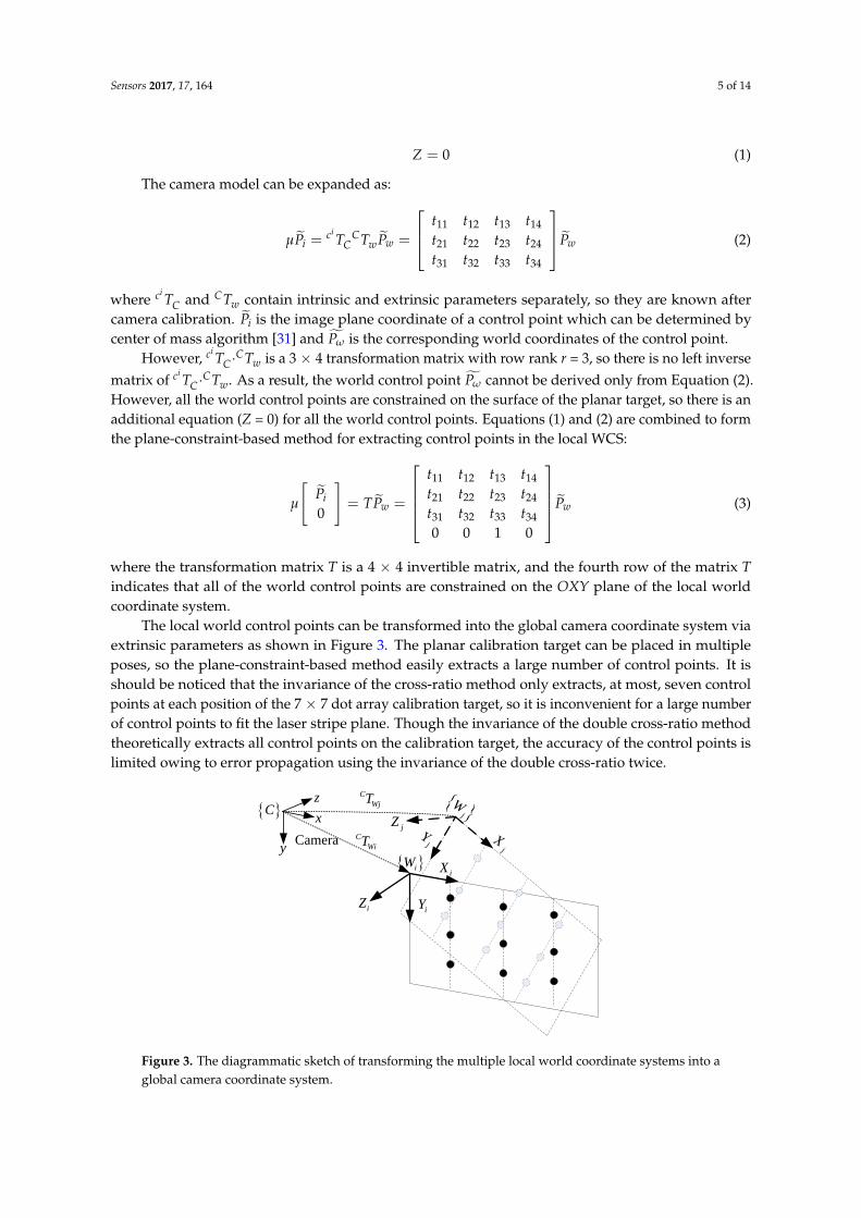
The local world control points can be transformed into the global camera coordinate system viaextrinsic parameters as shown in Figure 3. The planar calibration target can be placed in multipleposes, so the plane-constraint-based method easily extracts a large number of control points. It isshould be noticed that the invariance of the cross-ratio method only extracts, at most, seven controlpoints at each position of the 7 × 7 dot array calibration target, so it is inconvenient for a large numberof control points to fit the laser stripe plane. Though the invariance of the double cross-ratio methodtheoretically extracts all control points on the calibration target, the accuracy of the control points islimited owing to error propagation using the invariance of the double cross-ratio twice.

Sensors 2017, 17, 164 5 of 14

The camera model can be expanded as:

11 12 13 14

21 22 23 24

31 32 33 34

ic C

i C w w w

t t t t

P T T P t t t t P

t t t t

(2)

where 𝑇 𝑐𝑖

𝐶 and 𝑇 𝐶

𝑤 contain intrinsic and extrinsic parameters separately, so they are known after

camera calibration. 𝑃�� is the image plane coordinate of a control point which can be determined by

center of mass algorithm [31] and 𝑃�� is the corresponding world coordinates of the control point.

However, 𝑇 𝑐𝑖

𝐶 ∙ 𝑇 𝐶

𝑤 is a 3 × 4 transformation matrix with row rank r = 3, so there is no left inverse

matrix of 𝑇 𝑐𝑖

𝐶 ∙ 𝑇 𝐶

𝑤. As a result, the world control point 𝑃�� cannot be derived only from Equation

(2). However, all the world control points are constrained on the surface of the planar target, so there

is an additional equation (Z = 0) for all the world control points. Equations (1) and (2) are combined

to form the plane-constraint-based method for extracting control points in the local WCS:

11 12 13 14

21 22 23 24

31 32 33 340

0 0 1 0

i

w w

t t t t

t t t tPTP P

t t t t

(3)

where the transformation matrix T is a 4 × 4 invertible matrix, and the fourth row of the matrix T

indicates that all of the world control points are constrained on the OXY plane of the local world

coordinate system.

The local world control points can be transformed into the global camera coordinate system via

extrinsic parameters as shown in Figure 3. The planar calibration target can be placed in multiple

poses, so the plane-constraint-based method easily extracts a large number of control points. It is

should be noticed that the invariance of the cross-ratio method only extracts, at most, seven control

points at each position of the 7 × 7 dot array calibration target, so it is inconvenient for a large number

of control points to fit the laser stripe plane. Though the invariance of the double cross-ratio method

theoretically extracts all control points on the calibration target, the accuracy of the control points is

limited owing to error propagation using the invariance of the double cross-ratio twice.

iZ

C

WiT

iWiX

iY

jW

jX

jY

z C

Camera

x

y

jZ

C

WjT

Figure 3. The diagrammatic sketch of transforming the multiple local world coordinate systems into

a global camera coordinate system.

Figure 3. The diagrammatic sketch of transforming the multiple local world coordinate systems into aglobal camera coordinate system.

Sensors 2017, 17, 164 6 of 14

3.3. Mathematical Model of the Galvanometric Laser Scanner

The laser line projector can be modeled as a plane equation and the reflective mirror also can bemodeled as a plane equation. The rotational axis of the galvanometric is represented by a spatial line.What is more, all of the equations are expressed in the CCS.

3.3.1. Mathematical Model of Basic Elements

The plane ∏p equation of the laser line projector (incoming laser plane) is given below

apxc + bpyc + cpzc + dp = 0 (4)

where(ap, bp, cp, dp

)are the estimated plane parameters and np =

(ap, bp, cp

)are the normal vector

of the plane.The original plane ∏0 equation of the reflective mirror is:

a0xc + b0yc + c0zc + d0 = 0 (5)

The rotational axis l of the galvanometer element is expressed using the directional vector ω anda point P on l.

It is should be noticed that there are 11 independent parameters to describe two planes andone spatial line, and no position assumptions are made during the mathematical model of the basicelements. Consequently, machining and assembly errors, which affect the position of basic elements,are considered in the mathematical model. Meanwhile, the position of the laser projector is fixed in theCCS, so the plane equation of the laser line projector is fixed, but unknown, and the equation of thereflective mirror changes along with the rotation of the galvanometer element.

3.3.2. Equation of the Rotated Reflective Mirror

Based on screw theory [32], the transformation matrix T of the rotational axis l can be easilyexpressed as follows, and the twist coordinates ξ for the rotational axis l is given below:

ξ =[

v ω]T

(6)

v = −ω× P = −ωP (7)

where ω is the directional vector of l and P =(

Px, Py, Pz)

is a point on l.The operator, ∧ (wedge), forms a R4 × 4 matrix (the twist ξ ) out of a given vector ξ in R6:

ξ =

[vω

]Λ

=

[ω v

01×3 0

](8)

Then the transformation matrix T can be expressed via the exponential map from the twist ξ:

T = eξθ =

[eωθ

(I − eωθ

)(ω× v)

01×3 0

](9)

If the rotational angle θ of the galvanometer element is given, the transformation matrix T isdetermined. The equation of the rotated reflective mirror ∏i at the given θi can be easily expressedas follows:

ni = eξθi n0 (10)

Pi = eξθi P0 (11)

Sensors 2017, 17, 164 7 of 14

where n0 = [a0, b0, c0, 0]T is the homogeneous coordinate of the original reflective mirror’s normalvector in the CCS, and P0 =

[P0x, P0y, P0z, 1

]T is the homogeneous coordinate of the point P0 on theoriginal plane ∏0.

3.3.3. Equation of the Reflected Laser Plane

If the incoming laser plane ∏p and the rotated reflective plane ∏i are determined, the equation ofthe reflected laser plane can be given below.

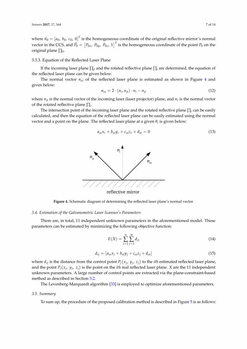
The normal vector noi of the reflected laser plane is estimated as shown in Figure 4 andgiven below:

noi = 2 · (ni, np) · ni − np (12)

where np is the normal vector of the incoming laser (laser projector) plane, and ni is the normal vectorof the rotated reflective plane ∏i.

The intersection point of the incoming laser plane and the rotated reflective plane ∏i can be easilycalculated, and then the equation of the reflected laser plane can be easily estimated using the normalvector and a point on the plane. The reflected laser plane at a given θi is given below:

aoixc + boiyc + coizc + doi = 0 (13)

Sensors 2017, 17, 164 7 of 14

where 𝑛0 = [𝑎0, 𝑏0, 𝑐0, 0]𝑇 is the homogeneous coordinate of the original reflective mirror’s normal

vector in the CCS, and 𝑃0 = [𝑃0𝑥, 𝑃0𝑦, 𝑃0𝑧, 1]𝑇 is the homogeneous coordinate of the point 𝑃0 on the

original plane ∏0.

3.3.3. Equation of the Reflected Laser Plane

If the incoming laser plane ∏p and the rotated reflective plane ∏i are determined, the equation of

the reflected laser plane can be given below.

The normal vector 𝑛𝑜𝑖 of the reflected laser plane is estimated as shown in Figure 4 and given

below:

2 ( , )oi i p i pn n n n n (12)

where 𝑛𝑝 is the normal vector of the incoming laser (laser projector) plane, and 𝑛𝑖 is the normal

vector of the rotated reflective plane ∏i.

The intersection point of the incoming laser plane and the rotated reflective plane ∏i can be easily

calculated, and then the equation of the reflected laser plane can be easily estimated using the normal

vector and a point on the plane. The reflected laser plane at a given 𝜃𝑖 is given below:

0oi c oi c oi c oia x b y c z d (13)

reflective mirror

pnin

oin

Figure 4. Schematic diagram of determining the reflected laser plane’s normal vector.

3.4. Estimation of the Galvanometric Laser Scanner’s Parameters

There are, in total, 11 independent unknown parameters in the aforementioned model. These

parameters can be estimated by minimizing the following objective function:

1 1

( )n m

ij

i j

E X d

(14)

ij oi j oi j oi j oid a x b y c z d (15)

where 𝑑𝑖𝑗 is the distance from the control point 𝑃𝑗(𝑥𝑗 , 𝑦𝑗 , 𝑧𝑗) to the ith estimated reflected laser

plane, and the point 𝑃𝑗(𝑥𝑗, 𝑦𝑗 , 𝑧𝑗) is the point on the ith real reflected laser plane. X are the 11

independent unknown parameters. A large number of control points are extracted via the plane-

constraint-based method as described in Section 3.2.

The Levenberg-Marquardt algorithm [33] is employed to optimize aforementioned parameters.

3.5. Summary

To sum up, the procedure of the proposed calibration method is described in Figure 5 is as

follows:

Figure 4. Schematic diagram of determining the reflected laser plane’s normal vector.

3.4. Estimation of the Galvanometric Laser Scanner’s Parameters

There are, in total, 11 independent unknown parameters in the aforementioned model. Theseparameters can be estimated by minimizing the following objective function:

E(X) =n

∑i=1

m

∑j=1

dij (14)

dij =∣∣aoixj + boiyj + coizj + doi

∣∣ (15)

where dij is the distance from the control point Pj(xj, yj, zj

)to the ith estimated reflected laser plane,

and the point Pj(

xj, yj, zj)

is the point on the ith real reflected laser plane. X are the 11 independentunknown parameters. A large number of control points are extracted via the plane-constraint-basedmethod as described in Section 3.2.

The Levenberg-Marquardt algorithm [33] is employed to optimize aforementioned parameters.

3.5. Summary

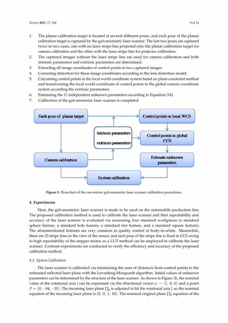
To sum up, the procedure of the proposed calibration method is described in Figure 5 is as follows:

Sensors 2017, 17, 164 8 of 14

1. The planar calibration target is located at several different poses, and each pose of the planarcalibration target is captured by the galvanometric laser scanner. The last two poses are capturedtwice in two cases, one with no laser stripe line projected onto the planar calibration target forcamera calibration and the other with the laser stripe line for projector calibration.

2. The captured images without the laser stripe line are used for camera calibration and bothintrinsic parameters and extrinsic parameters are determined.

3. Extracting all image coordinates of control points in two captured images.4. Correcting distortion for those image coordinates according to the lens distortion model.5. Calculating control points in the local world coordinate system based on plane-constraint method

and transforming the local world coordinate of control points to the global camera coordinatesystem according the extrinsic parameters.

6. Estimating the 11 independent unknown parameters according to Equation (14).7. Calibration of the galvanometric laser scanner is completed.

Sensors 2017, 17, 164 8 of 14

1. The planar calibration target is located at several different poses, and each pose of the planar

calibration target is captured by the galvanometric laser scanner. The last two poses are captured

twice in two cases, one with no laser stripe line projected onto the planar calibration target for

camera calibration and the other with the laser stripe line for projector calibration.

2. The captured images without the laser stripe line are used for camera calibration and both

intrinsic parameters and extrinsic parameters are determined.

3. Extracting all image coordinates of control points in two captured images.

4. Correcting distortion for those image coordinates according to the lens distortion model.

5. Calculating control points in the local world coordinate system based on plane-constraint

method and transforming the local world coordinate of control points to the global camera

coordinate system according the extrinsic parameters.

6. Estimating the 11 independent unknown parameters according to Equation (14).

7. Calibration of the galvanometric laser scanner is completed.

Figure 5. Flowchart of the one-mirror galvanometric laser scanner calibration procedures.

4. Experiments

Here, the galvanometric laser scanner is made to be used on the automobile production line. The

proposed calibration method is used to calibrate the laser scanner and then repeatability and accuracy

of the laser scanner is evaluated via measuring four standard workpieces (a standard sphere feature,

a standard hole feature, a standard slot feature, and a standard square feature). The aforementioned

features are very common in quality control of body-in-white. Meanwhile, there are 23 stripe lines in

the view of the sensor, and each pose of the stripe line is fixed in CCS owing to high repeatability of

the stepper motor, so a LUT method can be employed to calibrate the laser scanner. Contrast

experiments are conducted to verify the efficiency and accuracy of the proposed calibration method.

4.1. System Calibration

The laser scanner is calibrated via minimizing the sum of distances from control points to the

estimated reflected laser plane with the Levenberg-Marquardt algorithm. Initial values of unknown

parameters can be determined by the structure of the laser scanner. As shown in Figure 1b, the

nominal value of the rotational axis l can be expressed via the directional vector 𝜔 = (1, 0, 0) and a

point 𝑃 = (0, −94, −10). The incoming laser plane ∏p is adjusted to hit the rotational axis l, so the

nominal equation of the incoming laser plane is (0, 0, 1, 10). The nominal original plane ∏0 equation

of the reflective mirror can be determined by the incoming laser plane and the reflected laser plane,

so the nominal equation of the plane ∏0 is (0, 0.853, 0.477, 87). The aforementioned parameters are

Figure 5. Flowchart of the one-mirror galvanometric laser scanner calibration procedures.

4. Experiments

Here, the galvanometric laser scanner is made to be used on the automobile production line.The proposed calibration method is used to calibrate the laser scanner and then repeatability andaccuracy of the laser scanner is evaluated via measuring four standard workpieces (a standardsphere feature, a standard hole feature, a standard slot feature, and a standard square feature).The aforementioned features are very common in quality control of body-in-white. Meanwhile,there are 23 stripe lines in the view of the sensor, and each pose of the stripe line is fixed in CCS owingto high repeatability of the stepper motor, so a LUT method can be employed to calibrate the laserscanner. Contrast experiments are conducted to verify the efficiency and accuracy of the proposedcalibration method.

4.1. System Calibration

The laser scanner is calibrated via minimizing the sum of distances from control points to theestimated reflected laser plane with the Levenberg-Marquardt algorithm. Initial values of unknownparameters can be determined by the structure of the laser scanner. As shown in Figure 1b, the nominalvalue of the rotational axis l can be expressed via the directional vector ω = (1, 0, 0) and a pointP = (0,−94,−10). The incoming laser plane ∏p is adjusted to hit the rotational axis l, so the nominalequation of the incoming laser plane is (0, 0, 1, 10). The nominal original plane ∏0 equation of the

Sensors 2017, 17, 164 9 of 14

reflective mirror can be determined by the incoming laser plane and the reflected laser plane, so thenominal equation of the plane ∏0 is (0, 0.853, 0.477, 87). The aforementioned parameters are goodinitial guesses for the Levenberg-Marquardt algorithm. The laser scanner is calibrated according to thecalibration procedure described in Section 3.5.

4.2. Repeatability Evaluation

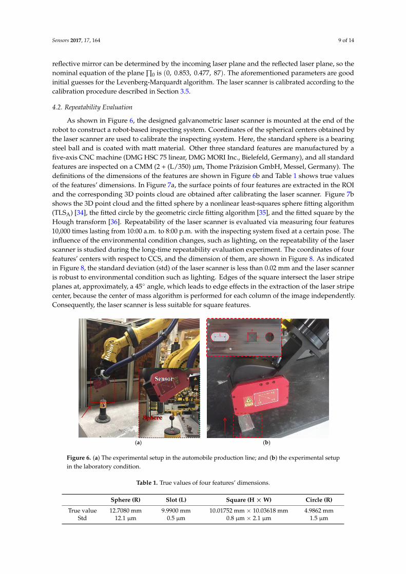
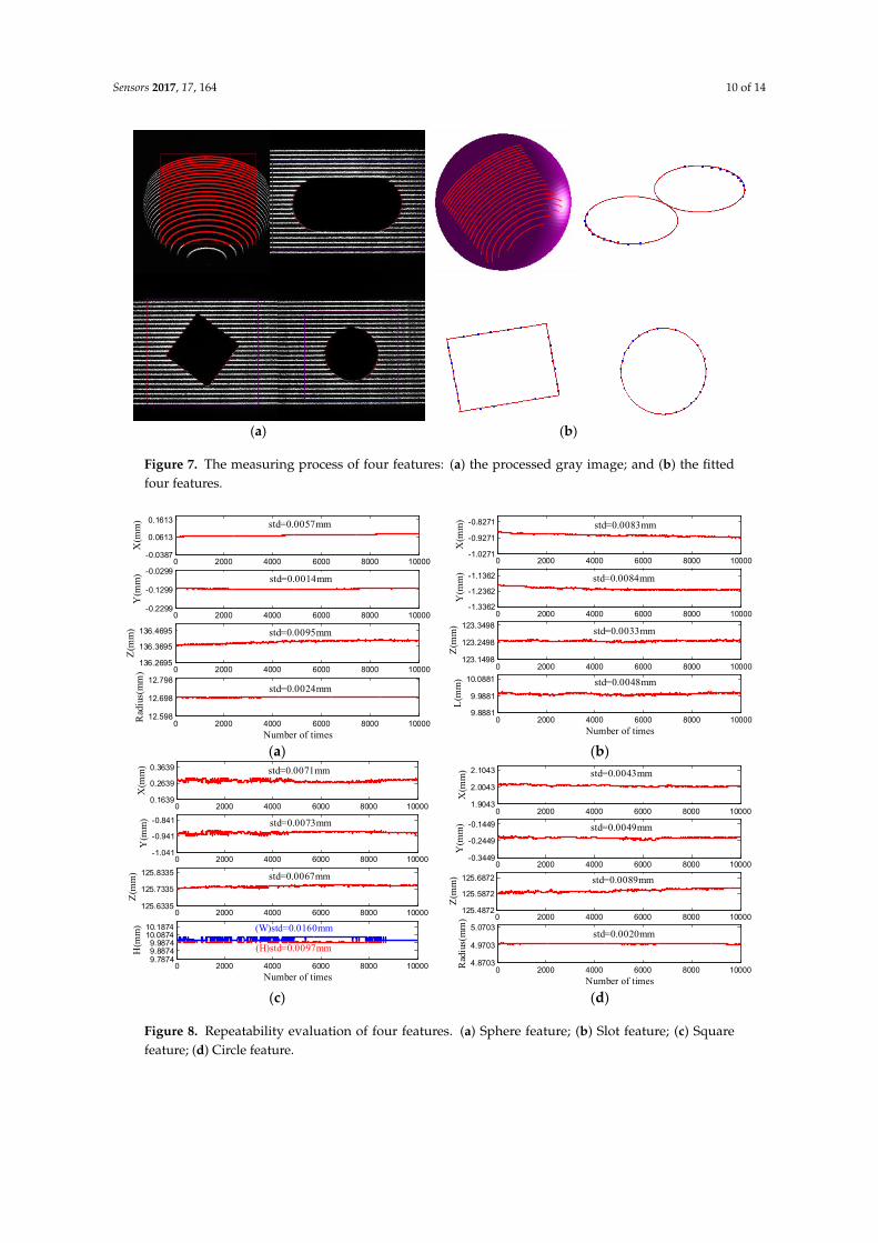
As shown in Figure 6, the designed galvanometric laser scanner is mounted at the end of therobot to construct a robot-based inspecting system. Coordinates of the spherical centers obtained bythe laser scanner are used to calibrate the inspecting system. Here, the standard sphere is a bearingsteel ball and is coated with matt material. Other three standard features are manufactured by afive-axis CNC machine (DMG HSC 75 linear, DMG MORI Inc., Bielefeld, Germany), and all standardfeatures are inspected on a CMM (2 + (L/350) µm, Thome Präzision GmbH, Messel, Germany). Thedefinitions of the dimensions of the features are shown in Figure 6b and Table 1 shows true valuesof the features’ dimensions. In Figure 7a, the surface points of four features are extracted in the ROIand the corresponding 3D points cloud are obtained after calibrating the laser scanner. Figure 7bshows the 3D point cloud and the fitted sphere by a nonlinear least-squares sphere fitting algorithm(TLSA) [34], the fitted circle by the geometric circle fitting algorithm [35], and the fitted square by theHough transform [36]. Repeatability of the laser scanner is evaluated via measuring four features10,000 times lasting from 10:00 a.m. to 8:00 p.m. with the inspecting system fixed at a certain pose. Theinfluence of the environmental condition changes, such as lighting, on the repeatability of the laserscanner is studied during the long-time repeatability evaluation experiment. The coordinates of fourfeatures’ centers with respect to CCS, and the dimension of them, are shown in Figure 8. As indicatedin Figure 8, the standard deviation (std) of the laser scanner is less than 0.02 mm and the laser scanneris robust to environmental condition such as lighting. Edges of the square intersect the laser stripeplanes at, approximately, a 45◦ angle, which leads to edge effects in the extraction of the laser stripecenter, because the center of mass algorithm is performed for each column of the image independently.Consequently, the laser scanner is less suitable for square features.

Sensors 2017, 17, 164 9 of 14

good initial guesses for the Levenberg-Marquardt algorithm. The laser scanner is calibrated

according to the calibration procedure described in Section 3.5.

4.2. Repeatability Evaluation

As shown in Figure 6, the designed galvanometric laser scanner is mounted at the end of the

robot to construct a robot-based inspecting system. Coordinates of the spherical centers obtained by the

laser scanner are used to calibrate the inspecting system. Here, the standard sphere is a bearing steel

ball and is coated with matt material. Other three standard features are manufactured by a five-axis

CNC machine (DMG HSC 75 linear, DMG MORI Inc., Bielefeld, Germany), and all standard features

are inspected on a CMM (2 + (L/350) μm, Thome Präzision GmbH, Messel, Germany). The definitions

of the dimensions of the features are shown in Figure 6b and Table 1 shows true values of the features’

dimensions. In Figure 7a, the surface points of four features are extracted in the ROI and the

corresponding 3D points cloud are obtained after calibrating the laser scanner. Figure 7b shows the

3D point cloud and the fitted sphere by a nonlinear least-squares sphere fitting algorithm (TLSA) [34],

the fitted circle by the geometric circle fitting algorithm [35], and the fitted square by the Hough

transform [36]. Repeatability of the laser scanner is evaluated via measuring four features 10,000

times lasting from 10:00 a.m. to 8:00 p.m. with the inspecting system fixed at a certain pose. The

influence of the environmental condition changes, such as lighting, on the repeatability of the laser

scanner is studied during the long-time repeatability evaluation experiment. The coordinates of

four features’ centers with respect to CCS, and the dimension of them, are shown in Figure 8. As

indicated in Figure 8, the standard deviation (std) of the laser scanner is less than 0.02 mm and the

laser scanner is robust to environmental condition such as lighting. Edges of the square intersect the

laser stripe planes at, approximately, a 45° angle, which leads to edge effects in the extraction of the

laser stripe center, because the center of mass algorithm is performed for each column of the image

independently. Consequently, the laser scanner is less suitable for square features.

(a) (b)

Figure 6. (a) The experimental setup in the automobile production line; and (b) the experimental setup

in the laboratory condition.

Table 1. True values of four features’ dimensions.

Sphere (R) Slot (L) Square (H × W) Circle (R)

True value 12.7080 mm 9.9900 mm 10.01752 mm × 10.03618 mm 4.9862 mm

Std 12.1 μm 0.5 μm 0.8 μm × 2.1 μm 1.5 μm

Figure 6. (a) The experimental setup in the automobile production line; and (b) the experimental setupin the laboratory condition.

Table 1. True values of four features’ dimensions.

Sphere (R) Slot (L) Square (H × W) Circle (R)

True value 12.7080 mm 9.9900 mm 10.01752 mm × 10.03618 mm 4.9862 mmStd 12.1 µm 0.5 µm 0.8 µm × 2.1 µm 1.5 µm

Sensors 2017, 17, 164 10 of 14

Sensors 2017, 17, 164 10 of 14

(a) (b)

Figure 7. The measuring process of four features: (a) the processed gray image; and (b) the fitted four

features.

(a) (b)

(c) (d)

Figure 8. Repeatability evaluation of four features. (a) Sphere feature; (b) Slot feature; (c) Square

feature; (d) Circle feature.

4.3. Accuracy Evaluation

Here, accuracy of the laser scanner is evaluated via measuring four features from six different

poses. The proposed calibration method is compared with other three calibration methods, such as

a one-step calibration method (Huynh [19]), a two-step calibration method (Zhou [21]) and other

0 2000 4000 6000 8000 10000-0.0387

0.0613

0.1613

X(m

m) std=0.0057mm

0 2000 4000 6000 8000 10000-0.2299

-0.1299

-0.0299

Y(m

m) std=0.0014mm

0 2000 4000 6000 8000 10000136.2695

136.3695

136.4695

Z(m

m) std=0.0095mm

0 2000 4000 6000 8000 1000012.598

12.698

12.798

Rad

ius(

mm

)

Number of times

std=0.0024mm

0 2000 4000 6000 8000 10000-1.0271

-0.9271

-0.8271

X(m

m)

std=0.0083mm

0 2000 4000 6000 8000 10000-1.3362

-1.2362

-1.1362

Y(m

m)

std=0.0084mm

0 2000 4000 6000 8000 10000123.1498

123.2498

123.3498

Z(m

m)

std=0.0033mm

0 2000 4000 6000 8000 100009.8881

9.9881

10.0881

L(m

m)

Number of times

std=0.0048mm

0 2000 4000 6000 8000 100000.1639

0.2639

0.3639

X(m

m) std=0.0071mm

0 2000 4000 6000 8000 10000-1.041

-0.941

-0.841

Y(m

m) std=0.0073mm

0 2000 4000 6000 8000 10000125.6335

125.7335

125.8335

Z(m

m) std=0.0067mm

0 2000 4000 6000 8000 100009.78749.88749.9874

10.087410.1874

H(m

m)

Number of times

(H)std=0.0097mm

(W)std=0.0160mm

0 2000 4000 6000 8000 100001.9043

2.0043

2.1043

X(m

m) std=0.0043mm

0 2000 4000 6000 8000 10000-0.3449

-0.2449

-0.1449

Y(m

m) std=0.0049mm

0 2000 4000 6000 8000 10000125.4872

125.5872

125.6872

Z(m

m) std=0.0089mm

0 2000 4000 6000 8000 100004.8703

4.9703

5.0703

Rad

ius(

mm

)

Number of times

std=0.0020mm

Figure 7. The measuring process of four features: (a) the processed gray image; and (b) the fittedfour features.

Sensors 2017, 17, 164 10 of 14

(a) (b)

Figure 7. The measuring process of four features: (a) the processed gray image; and (b) the fitted four features.

(a) (b)

(c) (d)

Figure 8. Repeatability evaluation of four features. (a) Sphere feature; (b) Slot feature; (c) Square feature; (d) Circle feature.

4.3. Accuracy Evaluation

Here, accuracy of the laser scanner is evaluated via measuring four features from six different poses. The proposed calibration method is compared with other three calibration methods, such as a one-step calibration method (Huynh [19]), a two-step calibration method (Zhou [21]) and other

0 2000 4000 6000 8000 10000-0.0387

0.0613

0.1613

X(m

m) std=0.0057mm

0 2000 4000 6000 8000 10000-0.2299

-0.1299

-0.0299

Y(m

m) std=0.0014mm

0 2000 4000 6000 8000 10000136.2695

136.3695

136.4695

Z(m

m) std=0.0095mm

0 2000 4000 6000 8000 1000012.598

12.698

12.798

Rad

ius(

mm

)

Number of times

std=0.0024mm

0 2000 4000 6000 8000 10000-1.0271

-0.9271

-0.8271

X(m

m) std=0.0083mm

0 2000 4000 6000 8000 10000-1.3362

-1.2362

-1.1362

Y(m

m) std=0.0084mm

0 2000 4000 6000 8000 10000123.1498

123.2498

123.3498

Z(m

m) std=0.0033mm

0 2000 4000 6000 8000 100009.8881

9.9881

10.0881

L(m

m)

Number of times

std=0.0048mm

0 2000 4000 6000 8000 100000.1639

0.2639

0.3639

X(m

m) std=0.0071mm

0 2000 4000 6000 8000 10000-1.041

-0.941

-0.841

Y(m

m) std=0.0073mm

0 2000 4000 6000 8000 10000125.6335

125.7335

125.8335

Z(m

m) std=0.0067mm

0 2000 4000 6000 8000 100009.78749.88749.9874

10.087410.1874

H(m

m)

Number of times

(H)std=0.0097mm

(W)std=0.0160mm

0 2000 4000 6000 8000 100001.9043

2.0043

2.1043

X(m

m) std=0.0043mm

0 2000 4000 6000 8000 10000-0.3449

-0.2449

-0.1449

Y(m

m) std=0.0049mm

0 2000 4000 6000 8000 10000125.4872

125.5872

125.6872

Z(m

m) std=0.0089mm

0 2000 4000 6000 8000 100004.8703

4.9703

5.0703

Rad

ius(

mm

)

Number of times

std=0.0020mm

Figure 8. Repeatability evaluation of four features. (a) Sphere feature; (b) Slot feature; (c) Squarefeature; (d) Circle feature.

Sensors 2017, 17, 164 11 of 14

4.3. Accuracy Evaluation

Here, accuracy of the laser scanner is evaluated via measuring four features from six differentposes. The proposed calibration method is compared with other three calibration methods, such asa one-step calibration method (Huynh [19]), a two-step calibration method (Zhou [21]) and othertwo-step calibration method (plane-constraint-based method). The aforementioned three calibrationmethods only deal with the vision sensor calibration problem with a fixed light stripe plane. However,there are 23 stripe lines in the view of the sensor, and each pose of the stripe line is fixed in theCCS owing to the high repeatability of the stepper motor. Inspired by LUT, three other calibrationmethods are repeated 23 times at each pose of the laser stripe plane to complete the calibration of thegalvanometric laser scanner and Zhou’s method stands for Zhou’s method with LUT in later paragraphand so on. The LUT method consists of two parts: (1) storing calibration matrices for 23 pre-definedlaser planes in a LUT; and (2) usage of the calibration matrix at a pre-defined rotational angle for 3Dreconstruction. The LUT method is used as a reference for the proposed model-driven calibrationmethod. Four calibration methods use the same calibration images to complete the calibrationprocedure and accuracy verification.

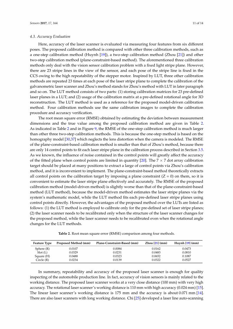
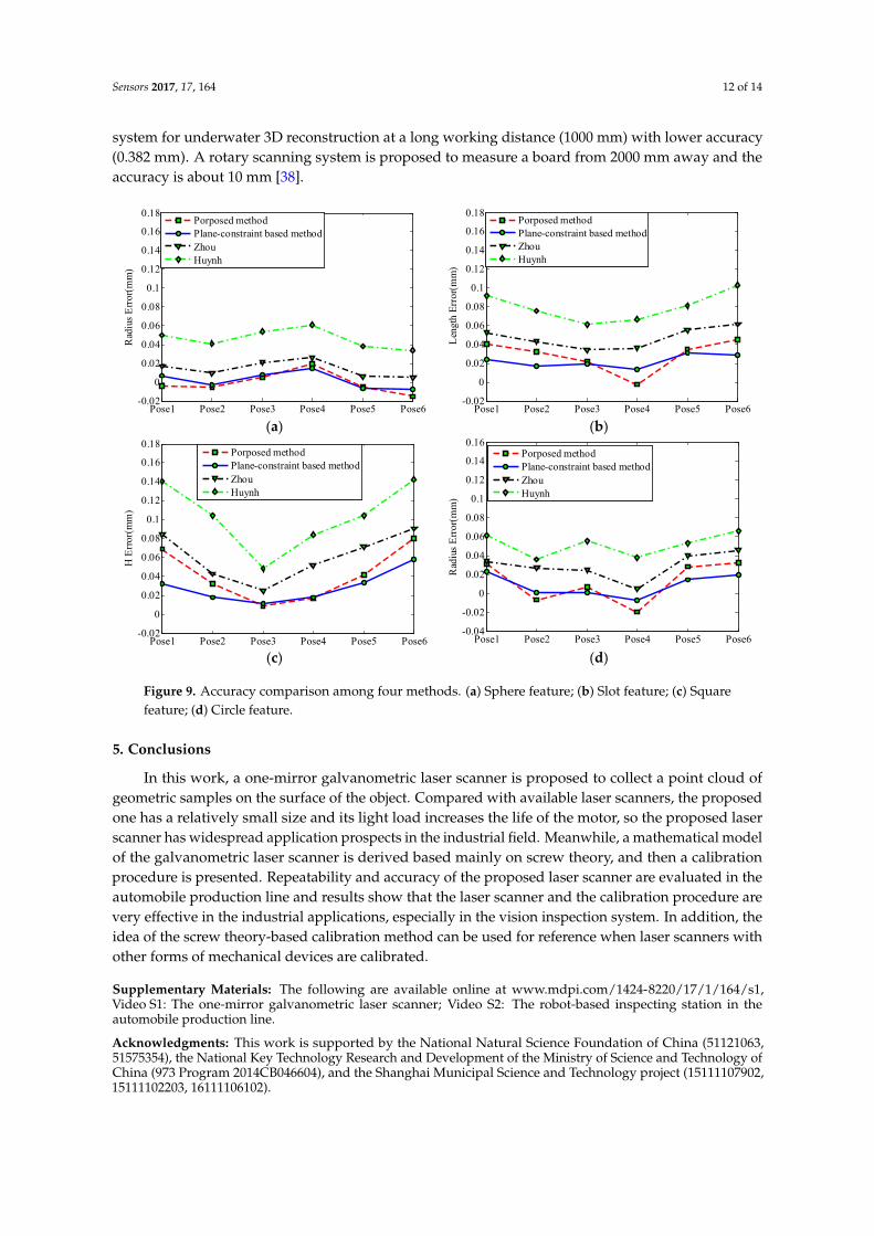
The root mean square error (RMSE) obtained by estimating the deviation between measurementdimensions and the true value among the proposed calibration method are given in Table 2.As indicated in Table 2 and in Figure 9, the RMSE of the one-step calibration method is much largerthan other three two-step calibration methods. This is because the one-step method is based on thehomography model [30,37] which neglects the lens distortion when the camera is modeled. The RMSEof the plane-constraint-based calibration method is smaller than that of Zhou’s method, because thereare only 14 control points to fit each laser stripe plane in the calibration process described in Section 3.5.As we known, the influence of noise contained in the control points will greatly affect the accuracyof the fitted plane when control points are limited in quantity [20]. The 7 × 7 dot array calibrationtarget should be placed at many positions to extract a large of control points via Zhou’s calibrationmethod, and it is inconvenient to implement. The plane-constraint-based method theoretically extractsall control points on the calibration target by imposing a plane constraint (Z = 0) on them, so it isconvenient to estimate the laser stripe plane effectively and accurately. The RMSE of the proposedcalibration method (model-driven method) is slightly worse than that of the plane-constraint-basedmethod (LUT method), because the model-driven method estimates the laser stripe planes via thesystem’s mathematic model, while the LUT method fits each pre-defined laser stripe planes usingcontrol points directly. However, the advantages of the proposed method over the LUTs are listed asfollows: (1) the LUT method is employed to calibrate only for the pre-defined set of laser stripe planes;(2) the laser scanner needs to be recalibrated only when the structure of the laser scanner changes forthe proposed method, while the laser scanner needs to be recalibrated even when the rotational anglechanges for the LUT methods.

Table 2. Root mean square error (RMSE) comparison among four methods.

Feature Type Proposed Method (mm) Plane-Constraint-Based (mm) Zhou [21] (mm) Huynh [19] (mm)

Sphere (R) 0.0107 0.0084 0.0162 0.0473Slot (L) 0.0329 0.0231 0.0483 0.0810

Square (H) 0.0488 0.0323 0.0652 0.1087Circle (R) 0.0234 0.0139 0.0322 0.0527

In summary, repeatability and accuracy of the proposed laser scanner is enough for qualityinspecting of the automobile production line. In fact, accuracy of vision sensors is mainly related to theworking distance. The proposed laser scanner works at a very close distance (100 mm) with very highaccuracy. The rotational laser scanner’s working distance is 110 mm with high accuracy (0.024 mm) [15].The linear laser scanner’s working distance is 175 mm and the accuracy is about 0.071 mm [14].There are also laser scanners with long working distance. Chi [25] developed a laser line auto-scanning

Sensors 2017, 17, 164 12 of 14

system for underwater 3D reconstruction at a long working distance (1000 mm) with lower accuracy(0.382 mm). A rotary scanning system is proposed to measure a board from 2000 mm away and theaccuracy is about 10 mm [38].Sensors 2017, 17, 164 12 of 14

(a) (b)

(c) (d)

Figure 9. Accuracy comparison among four methods. (a) Sphere feature; (b) Slot feature; (c) Square feature; (d) Circle feature.

5. Conclusions

In this work, a one-mirror galvanometric laser scanner is proposed to collect a point cloud of geometric samples on the surface of the object. Compared with available laser scanners, the proposed one has a relatively small size and its light load increases the life of the motor, so the proposed laser scanner has widespread application prospects in the industrial field. Meanwhile, a mathematical model of the galvanometric laser scanner is derived based mainly on screw theory, and then a calibration procedure is presented. Repeatability and accuracy of the proposed laser scanner are evaluated in the automobile production line and results show that the laser scanner and the calibration procedure are very effective in the industrial applications, especially in the vision inspection system. In addition, the idea of the screw theory-based calibration method can be used for reference when laser scanners with other forms of mechanical devices are calibrated.

Supplementary Materials: The following are available online at www.mdpi.com/1424-8220/17/1/164/s1, Video S1: The one-mirror galvanometric laser scanner; Video S2: The robot-based inspecting station in the automobile production line.

Acknowledgments: This work is supported by the National Natural Science Foundation of China (51121063, 51575354), the National Key Technology Research and Development of the Ministry of Science and Technology of China (973 Program 2014CB046604), and the Shanghai Municipal Science and Technology project (15111107902, 15111102203, 16111106102).

Author Contributions: Chengyi Yu and Juntong Xi conceived and designed the experiments; Chengyi Yu and Xiaobo Chen performed the experiments; Chengyi Yu analyzed the data; Chengyi Yu and Xiaobo Chen wrote the paper.

Conflicts of Interest: The authors declare no conflict of interest.

Pose1 Pose2 Pose3 Pose4 Pose5 Pose6-0.02

0

0.02

0.04

0.06

0.08

0.1

0.12

0.14

0.16

0.18

Rad

ius E

rror(m

m)

Porposed methodPlane-constraint based methodZhouHuynh

Pose1 Pose2 Pose3 Pose4 Pose5 Pose6-0.02

0

0.02

0.04

0.06

0.08

0.1

0.12

0.14

0.16

0.18

Leng

th E

rror

(mm

)

Porposed methodPlane-constraint based methodZhouHuynh

Pose1 Pose2 Pose3 Pose4 Pose5 Pose6-0.02

0

0.02

0.04

0.06

0.08

0.1

0.12

0.14

0.16

0.18

H E

rror(

mm

)

Porposed methodPlane-constraint based methodZhouHuynh

Pose1 Pose2 Pose3 Pose4 Pose5 Pose6-0.04

-0.02

0

0.02

0.04

0.06

0.08

0.1

0.12

0.14

0.16R

adiu

s Erro

r(mm

)

Porposed methodPlane-constraint based methodZhouHuynh

Figure 9. Accuracy comparison among four methods. (a) Sphere feature; (b) Slot feature; (c) Squarefeature; (d) Circle feature.

5. Conclusions

In this work, a one-mirror galvanometric laser scanner is proposed to collect a point cloud ofgeometric samples on the surface of the object. Compared with available laser scanners, the proposedone has a relatively small size and its light load increases the life of the motor, so the proposed laserscanner has widespread application prospects in the industrial field. Meanwhile, a mathematical modelof the galvanometric laser scanner is derived based mainly on screw theory, and then a calibrationprocedure is presented. Repeatability and accuracy of the proposed laser scanner are evaluated in theautomobile production line and results show that the laser scanner and the calibration procedure arevery effective in the industrial applications, especially in the vision inspection system. In addition, theidea of the screw theory-based calibration method can be used for reference when laser scanners withother forms of mechanical devices are calibrated.

Supplementary Materials: The following are available online at www.mdpi.com/1424-8220/17/1/164/s1,Video S1: The one-mirror galvanometric laser scanner; Video S2: The robot-based inspecting station in theautomobile production line.

Acknowledgments: This work is supported by the National Natural Science Foundation of China (51121063,51575354), the National Key Technology Research and Development of the Ministry of Science and Technology ofChina (973 Program 2014CB046604), and the Shanghai Municipal Science and Technology project (15111107902,15111102203, 16111106102).

Sensors 2017, 17, 164 13 of 14

Author Contributions: Chengyi Yu and Juntong Xi conceived and designed the experiments; Chengyi Yu andXiaobo Chen performed the experiments; Chengyi Yu analyzed the data; Chengyi Yu and Xiaobo Chen wrotethe paper.

Conflicts of Interest: The authors declare no conflict of interest.

References

1. Zhang, L.; Wu, C.Y.; Zou, Y.Y. An on-line visual seam tracking sensor system during laser beam welding.In Proceedings of the International Conference on Information Technology and Computer Science, ITCS 2009,Kiev, Ukraine, 25–26 July 2009; pp. 361–364.

2. Huang, W.; Kovacevic, R. A laser-based vision system for weld quality inspection. Sensors 2011, 11, 506–521.[CrossRef]

3. Baeg, M.H.; Baeg, S.H.; Moon, C.; Jeong, G.M.; Ahn, H.S.; Kim, D.H. A new robotic 3D inspection system ofautomotive screw hole. Int. J. Control Autom. Syst. 2008, 6, 740–745.

4. Gan, Z.; Tang, Q. Visual Sensing and Its Applications: Integration of Laser Sensors to Industrial Robots; ZhejiangUniversity Press: Zhejiang, China; Springer: Berlin, Germany, 2011.

5. Li, J.F.; Guo, Y.K.; Zhu, J.H.; Lin, X.D.; Xin, Y.; Duan, K.L.; Tang, Q. Large depth-of-view portablethree-dimensional laser scanner and its segmental calibration for robot vision. Opt. Lasers Eng. 2007,45, 1077–1087. [CrossRef]

6. Li, J.F.; Zhu, J.H.; Guo, Y.K.; Lin, X.D.; Duan, K.L.; Wang, Y.S.; Tang, Q. Calibration of a portable laser 3-Dscanner used by a robot and its use in measurement. Opt. Eng. 2008, 47, 017202. [CrossRef]

7. Li, J.F.; Chen, M.; Jin, X.B.; Chen, Y.; Dai, Z.Y.; Ou, Z.H.; Tang, Q. Calibration of a multiple axes 3-Dlaser scanning system consisting of robot, portable laser scanner and turntable. Optik 2011, 122, 324–329.[CrossRef]

8. Xie, Z.; Wang, X.; Chi, S. Simultaneous calibration of the intrinsic and extrinsic parameters of structured-lightsensors. Opt. Lasers Eng. 2014, 58, 9–18. [CrossRef]

9. Abzal, A.; Varshosaz, M.; Saadatseresht, M. Development of a new laser triangulation system based on anoptical frame of reference. Photogramm. Record 2011, 26, 293–306. [CrossRef]

10. Zhang, Z.; Lin, Y. Building a 3D scanner system based on monocular vision. Appl. Opt. 2012, 51, 1638–1644.[CrossRef] [PubMed]

11. Furukawa, R.; Kawasaki, H. Laser range scanner based on self-calibration techniques using coplanaritiesand metric constraints. Comput. Vis. Image Underst. 2009, 113, 1118–1129. [CrossRef]

12. Ozan, S.; Gumustekin, S. Calibration of double stripe 3D laser scanner systems using planarity andorthogonality constraints. Digit. Signal Proc. 2014, 24, 231–243. [CrossRef]

13. Ren, Y.; Yin, S.; Zhu, J. Calibration technology in application of robot-laser scanning system. Opt. Eng. 2012,51, 114204. [CrossRef]

14. Yin, S.; Ren, Y.; Guo, Y.; Zhu, J.; Yang, S.; Ye, S. Development and calibration of an integrated 3D scanningsystem for high-accuracy large-scale metrology. Measurement 2014, 54, 65–76. [CrossRef]

15. Li, L.; Xi, J. Free and Global Pose Calibration of a Rotating Laser Monocular Vision Sensor for Robotic 3DMeasurement System. Proc. SPIE 2013, 8769. [CrossRef]

16. Xiao, J.; Hu, X.; Lu, W.; Ma, J.; Guo, X. A new three-dimensional laser scanner design and its performanceanalysis. Optik Int. J. Light Electron Opt. 2015, 126, 701–707. [CrossRef]

17. Liu, Z.; Li, X.; Li, F.; Zhang, G. Calibration method for line-structured light vision sensor based on a singleball target. Opt. Lasers Eng. 2015, 69, 20–28. [CrossRef]

18. Liu, Z.; Li, X.; Yin, Y. On-site calibration of line-structured light vision sensor in complex light environments.Opt. Express 2015, 23, 29896–29911. [CrossRef]

19. Huynh, D.Q.; Owens, R.A.; Hartmann, P. Calibrating a structured light stripe system: A novel approach.Int. J. Comput. Vis. 1999, 33, 73–86. [CrossRef]

20. Wei, Z.Z.; Zhang, G.J.; Xu, Y. Calibration approach for structured-light-stripe vision sensor based on theinvariance of double cross-ratio. Opt. Eng. 2003, 42, 2956–2966. [CrossRef]

21. Zhou, F.Q.; Zhang, G.J.; Jiang, J. Constructing feature points for calibrating a structured light vision sensorby viewing a plane from unknown orientations. Opt. Lasers Eng. 2005, 43, 1056–1070. [CrossRef]

Sensors 2017, 17, 164 14 of 14

22. Manakov, A.; Seidel, H.P.; Ihrke, I. A mathematical model and calibration procedure for galvanometric laserscanning systems. In Proceedings of the 16th Annual Workshop on Vision, Modeling, and Visualization,Berlin, Germany, 4–6 October 2011; pp. 348–357.

23. Wagner, B.; Stuber, P.; Wissel, T.; Bruder, R.; Schweikard, A.; Ernst, F. Accuracy analysis for triangulation andtracking based on time-multiplexed structured light. Med. Phys. 2014, 41, 082701. [CrossRef] [PubMed]

24. Wissel, T.; Wagner, B.; Stuber, P.; Schweikard, A. Data-driven learning for calibrating galvanometric laserscanners. IEEE Sens. J. 2015, 15, 5709–5717. [CrossRef]

25. Chi, S.; Xie, Z.; Chen, W. A laser line auto-scanning system for underwater 3D reconstruction. Sensors 2016,16, 1534. [CrossRef]

26. Perceptron. Tricam. Available online: http://perceptron.com/products/perceptron-sensor-technology/(accessed on 17 November 2016).

27. Tsai, R.Y. A versatile camera calibration technique for high-accuracy 3D machine vision metrology usingoff-the-shelf tv cameras and lenses. Robot. Autom. IEEE J. 1987, 3, 323–344. [CrossRef]

28. Heikkila, J.; Silven, O. A four-step camera calibration procedure with implicit image correction.In Proceedings of the 1997 IEEE Computer Society Conference on Computer Vision & Pattern Recognition,San Juan, Puerto Rico, 17–19 June 1997; pp. 1106–1112.

29. Zhang, Z. A flexible new technique for camera calibration. IEEE Trans. Pattern Anal. Mach. Intell. 2000, 22,1330–1334. [CrossRef]

30. Forest Collado, J. New Methods for Triangulation-Based Shape Acquisition Using Laser Scanners; Universitat deGirona: Girona, Spain, 2004.

31. Haug, K.; Pritschow, G. Robust laser-stripe sensor for automated weld-seam-tracking in the shipbuildingindustry. In Proceedings of the 24th Annual Conference of the IEEE Industrial Electronics Society, IECON’98,Aachen, Germany, 31 August–4 September 1998; pp. 1236–1241.

32. Murray, R.M.; Li, Z.; Sastry, S.S. A Mathematical Introduction to Robotic Manipulation; CRC Press: Boca Raton,FL, USA, 1994.

33. Moré, J.J. The levenberg-marquardt algorithm: Implementation and theory. In Numerical Analysis; Springer:Berlin, Germany, 1978; pp. 105–116.

34. Sun, W.J.; Hill, M.; McBride, J.W. An investigation of the robustness of the nonlinear least-squares spherefitting method to small segment angle surfaces. Precis. Eng. J. Int. Soc. Precis. Eng. Nanotechnol. 2008, 32,55–62. [CrossRef]

35. Chernov, N. Circular and Linear Regression: Fitting Circles and Lines by Least Squares; CRC Press: Boca Raton,FL, USA, 2010.

36. Illingworth, J.; Kittler, J. A survey of the hough transform. Comput. Vis. Graph. Image Proc. 1988, 44, 87–116.[CrossRef]

37. Niola, V.; Rossi, C.; Savino, S.; Strano, S. A method for the calibration of a 3-D laser scanner. Robot. Comput.Integr. Manuf. 2011, 27, 479–484. [CrossRef]

38. Nakatani, T.; Li, S.; Ura, T.; Bodenmann, A.; Sakamaki, T. 3D visual modeling of hydrothermal chimneysusing a rotary laser scanning system. In Proceedings of the 2011 IEEE Symposium on Underwater Technology(UT) and 2011 Workshop on Scientific Use of Submarine Cables and Related Technologies (SSC), Tokyo,Japan, 5–8 April 2011; pp. 1–5.

© 2017 by the authors; licensee MDPI, Basel, Switzerland. This article is an open accessarticle distributed under the terms and conditions of the Creative Commons Attribution(CC BY) license (http://creativecommons.org/licenses/by/4.0/).