modeling and analysis of ofdm with adaptive...

MODELING AND ANALYSIS OF OFDM WITHADAPTIVE CLIPPING TECHNIQUE FOR PAPR

REDUCTION

A THESIS SUBMITTED IN PARTIAL FULFILLMENT

OF THE REQUIREMENTS FOR THE DEGREE OF

Master of Technology

In

Telematics and Signal Processing

By

S VENKATESWARA RAO

20507031

Department of Electronics & Communication Engineering

National Institute of Technology

Rourkela

2007

MODELING AND ANALYSIS OF OFDM WITHADAPTIVE CLIPPING TECHNIQUE FOR PAPR

REDUCTION

A THESIS SUBMITTED IN PARTIAL FULFILLMENT

OF THE REQUIREMENTS FOR THE DEGREE OF

Master of Technology

In

Telematics and Signal Processing

By

S VENKATESWARA RAO

20507031

Under the Guidance of

Prof. K. K. Mahapathra

Dr. Sivannarayana Nagireddi

Department of Electronics & Communication Engineering

National Institute of Technology

Rourkela

2007

NATIONAL INSTITUTE OF TECHNOLOGYROURKELA

CERTIFICATE

This is to certify that the Thesis Report entitled “Modeling and Analysis of OFDM with

Adaptive Clipping Technique for PAPR Reduction” submitted by Mr. S Venkateswara Rao

(20507031) in partial fulfillment of the requirements for the award of Master of Technology

degree in Electronics and Communication Engineering with specialization in “Telematics and

Signal Processing” during session 2006-2007 at National Institute of Technology, Rourkela

(Deemed University) and is an authentic work by him under my supervision and guidance.

To the best of my knowledge, the matter embodied in the thesis has not been submitted to any

other university/institute for the award of any Degree or Diploma.

Prof. K. K. MAHAPATRADept. of E.C.E

Date: National Institute of TechnologyPlace: Rourkela-769008

Acknowledgements

With a profound sense of gratitude, I would like to express my heartfelt thanks to my project

guide Prof. K.K Mahapatra, Department of ECE, NIT Rourkela, for his constant support,

and encouragement throughout the project. His vast knowledge, patience, and valuable

advice helped me to accomplish this work successfully.

I would like to thank all my professors Dr G. Panda, Dr G. S. Rath, Dr S. K. Patra, and

Dr S. Meher for providing a solid background for my studies and research thereafter. They

have been great sources of inspiration to me and I thank them from the bottom of my heart.

I would like to take this privilege to express my deep sense of gratitude to Dr

Sivannarayana Nagireddi, Product Manager, DSP & VoIP Systems, Ikanos

Communications, for his valuable help and inspiring guidance that facilitated me to carry out

this work. I sincerely thank for his exemplary guidance and encouragement.

I would like to thank, Mr. Saiprasad Kalinga, and Mr. Vijay Shikhamani Kalakotla, DSP

Media Group, Ikanos Communications, for their constant guidance, support, encouragement,

in executing this project and making this success.

I would like to thank my friends Balaji, Jagan, Pradeep, Chaitanya, Suresh, and Rakesh

for their suggestions, guidelines and valuable help during my entire post graduation period.

I would like to thank all my friends and especially my classmates for all the thoughtful and

mind stimulating discussions we had, which prompted us to think beyond the obvious. I’ve

enjoyed their companionship so much during my stay at NIT, Rourkela.

Last but not least I would like to thank my parents, who taught me the value of hard work by

their own example. I would like to share this moment of happiness with my father and

mother. They rendered me enormous support during the whole tenure of my stay in NIT

Rourkela.

Venkateswara Rao Samineni

M.Tech (T& SP)

Contents

Chapter No Description Page No

Abstract i

List of Figures ii

List of Tables v

Legends vi

Abbreviations Used vii

Chapter 1 1 Introduction 1

1.1 Introduction 2

1.2 Motivation 2

1.3 Background Literature Survey 3

1.4 Thesis Contribution 5

1.5 Thesis Outline 5

Chapter 2 2 IEEE 802.11a, 802.11b, 802.11g WLANs 6

2.1 Introduction 7

2.2 The IEEE 802.11b Wireless Network Standard 8

2.3 The IEEE 802.11a Wireless Network Standard 10

2.3.1 Orthogonal Frequency Division Multiplexing Scheme 11

2.3.2 Eight Non Overlapping 20 MHz Channels 11

2.3.3 Forward Error Correction 13

2.3.4 Multipath Reflection 14

2.3.5 Data Rates and Ranges 14

2.3.6 The MAC Layer 802.11a 15

2.3.7 The Four way reliability method employed by 802.11a15

2.3.8 Compatibility and Inter Compatibility features of

802.11a with 802.11b 15

2.3.9 Transfer Rates and Distances of the versions of 802.1116

2.4 The IEEE 802.11g Wireless Network Standard 17

2.5 Comparing 802.11a, 802.11b, 802.11g Technologies 18

2.6 IEEE 802.11n Standard 19

2.7 Chapter Conclusion 20

Chapter 3 3 Modulation Schemes 21

3.1 Introduction 22

3.2 Phase Shift Keying 22

3.2.1 Binary Phase Shift Keying 23

3.2.2 Quadrature Phase Shift Keying 24

3.3 Quadrature Amplitude Modulation 25

3.4 Simulation Results 26


Chapter 4 4 Orthogonal Frequency Division Multiplexing 30

4.1 Introduction 31

4.2 Orthogonal Frequency Division Multiplexing 32

4.2.1 The importance of Orthogonality 32

4.2.2 Mathematical description of OFDM 33

4.3 The Fourier Transform 34

4.4 Signal Representation of OFDM using IFFT/FFT 35

4.5 Guard interval 37

4.6 Choice of the key elements 38

4.6.1 Useful symbol duration 38

4.6.2 Number of Carriers 38

4.6.3 Modulation Scheme 38

4.7 Advantages and Disadvantages of OFDM 39



Chapter 5 5 Reed Solomon Coded OFDM 42

5.1 Introduction 43

5.2 Encoding 44

5.3 Decoding 44

5.3.1 Syndrome Calculation 45

5.3.2 Error Polynomial Calculation using

Berlekamp Algorithm 45

5.3.3 Error Location Calculation using Chien Search 47

5.3.4 Error Magnitude Calculation using Forney Algorithm 47

5.3.5 Error Correction 48

5.4 OFDM with Reed Solomon Encoder and Decoder 48



Chapter 6 6 Adaptive Clipping Technique for reducing PAPR on OFDM 50

6.1 Introduction 51

6.2 PAPR Problem 51

6.2 System Model 51

6.3 PAPR Reduction Scheme 53



Chapter 7 7 RS coded OFDM for PAPR Technique 56

7.1 Introduction 57

7.2 System Model Used 57



Chapter 8 8 Conclusion 60

8.1 Achievement of thesis 61

8.2 Scope of further research 61

References 62

i

Abstract

Orthogonal Frequency Division Multiplexing (OFDM) systems are better than single-carrier

systems in multipath fading channel environment. OFDM systems are being adapted in many

wire-line and wireless high data rate transmission systems of digital video broadcasting

(DVB), IEEE 802.11, IEEE 802.16, HIPERLAN Type II, Digital Subscriber Line (DSL), and

Home networking etc. There is also strong interest to use OFDM systems in 4G wireless

systems.

OFDM has recently received increased attention due to its capability of supporting high data

rate communication in frequency selective fading environments which cause Inter symbol

Interference (ISI). In order to take advantage of the diversity provided by the multi-path

fading, appropriate frequency interleaving and coding is necessary. Therefore, coding

becomes an inseparable part in most OFDM applications and a considerable amount of

research has focused on optimum encoder and decoder design for information transmission

through OFDM over fading environments.

The OFDM systems use multiple orthogonal subcarriers. Transmission data is loaded on each

subcarrier and transmitted after summation. When all subcarriers have same phase than

instantaneous power of transmitted signal is very high. The peak power of OFDM scheme is

higher than average power. This phenomenon is called PAPR problem. This is one of the

main disadvantages of the OFDM system. Power amplifier characteristics are linear until

some input value, so for higher peak powers the amplifier characteristic may be nonlinear. If

peak powers are not handled in linear part, OFDM signals will get distorted. A definition of

PAPR is log-scale of peak power over average power, and PAPR problem appears in all

multicarrier systems. Traditionally several techniques are used for reducing PAPR instead of

catering for higher peak powers in amplifiers. First, clipping technique is the most famous

and simple technique. But it has BER (Bit Error Rate) performance degradation. Second,

peak power avoidance precoding technique is used. It has some coding gain but it decrease

data rate or increase bandwidth. Third, scrambling technique is used. With the scrambling

technique, probability of peak power occurrence goes low, but hardware architecture is more

complex.

ii

In this thesis, a joint solution is proposed with RS coding, OFDM, and PAPR clipping. We

implemented the hybrid method which consists of RS coding and adaptive clipping technique

over an additive white Gaussian noise (AWGN) channel. Reed Solomon RS (255, 239)

coding can correct 8 symbol errors from 239 symbols data. This capability can effectively

compensate for the performance degradation resulted by setting PAPR threshold to 5 in case

of 256 QAM, and RS (63, 47) and threshold of 4 incase of 64 QAM.

Binary data are grouped into ‘x’ bits and encoded by RS (255, 239) encoder and then

modulated by 256 QAM. For 64 QAM, RS (63, 47) is used. In a typical OFDM system

consists of N = 52 subcarriers and 64 point IFFT is used. The adaptive clipping technique is

used with clipping ratio of 5 for 256 QAM, and clipping ratio of 4 for 64 QAM is used. The

symbols are transmitted through AWGN channel. The receiver structure has reciprocal to the

transmitter architecture.

The implemented hybrid technique based on RS coding and adaptive clipping technique

method to compensate the performance degradation caused by clipping. From the simulation

results, by using hybrid technique the clipping distortion can be removed when CR = 5 and

SNR = 26.5 dB for 256 QAM, and CR = 4 and SNR = 20.5 dB for 64 QAM. The simulation

results show that the hybrid method is an effective technique to mitigate the clipping

distortions.

iii

List of Figures

Figure No Figure Title Page No

Figure 2.1 The IEEE 802.11Protocol Architecture Layer Model 7

Figure 2.2 The Complementary Code Keying Spreading Process 8

Figure 2.3 Multiple Users with Differentially Spread Signal 9

Figure 2.4 The three sub channels of the 802.11b WLAN 9

Figure 2.5 The Low, Medium, and High bands used by 802.11a 10

Figure 2.6 The 802.11a Low, Medium and High Frequency sub channels 12

Figure 2.7 For 802.11a, the eight channels are each composed of

52 sub channels 12

Figure 2.8 The 52 of 64 usable sub channels of 802.11a 13

Figure 2.9 The Effect of Multipath Signaling with Collisions 14

Figure 2.10 A Comparison of transmission distances and speeds for

802.11a and 802.11b 15

Figure 2.11 Various Speeds and Distances Achievable by 802.11 Networks 16

Figure 3.1 Change of phase with symbol change 23

Figure 3.2 Phase Shift Modulation Process 23

Figure 3.3 A Phase diagram showing the 0 and 180 degree phases 24

Figure 3.4 Quadrature Phase Shift Keying 24

Figure 3.5 Constellation Diagrams for 16 QAM 25

Figure 3.6 Constellation Diagrams for 256 QAM 25

Figure 3.7 Constellation diagrams, AWGN noisy Signals at different SNR, and

BER plot 256 QAM 27


BER plot 64 QAM 27


BER plot 16 QAM 28


BER plot 4 QAM 28

Figure 4.1 Functional band representations of FDM and OFDM 32

Figure 4.2 Block diagram of an OFDM system using FFT 36

iv

Figure 4.3 Examples of OFDM spectrum (a) a single subchannel,

(b) 5 carriers at the central frequency of each subchannel,

there is no crosstalk from other subchannels 36

Figure 4.4 The effect on the timing tolerance of adding a guard interval.

With a guard interval included in the signal, the tolerance

on timing the samples is considerably more 37

Figure 4.5 Example of the guard interval. Each symbol is made up of

two parts. The whole signal is contained in the active symbol,

The last part of which (shown in bold) is also repeated at the

start of the symbol and is called the guard interval 37

Figure 4.6 SNR v/s BER plots for OFDM system using subcarrier

modulation schemes 256 QAM, 64 QAM, 16 QAM and QPSK 40

Figure 5.1 Reed Solomon Encoder 44

Figure 5.2 Reed Solomon Decoder 45

Figure 5.3 Berlekamp Algorithm Flowchart 46

Figure 5.4 OFDM Simulation Model used 48

Figure 5.5 Comparison of OFDM and RS OFDM for 256 QAM 49

Figure 5.6 Comparison of OFDM and RS OFDM for 64 QAM 49

Figure 6.1 OFDM Simulation Model 52

Figure 6.2 SNR v/s BER plots for Adaptive clipped OFDM system for256 QAM at CR-4 and CR-5 54

Figure 6.3 SNR v/s BER plots for Adaptive clipped OFDM system for

64 QAM at CR-3 and CR-4 54

Figure 7.1 OFDM System Model used for Simulation 57

Figure 7.2 Comparison of OFDM, RS coded OFDM, PAPR Reduced OFDM,

and RS Coded OFDM for PAPR Technique for 256 QAM 58

Figure 7.3 Comparison of OFDM, RS coded OFDM, PAPR Reduced OFDM,and RS Coded OFDM for PAPR Technique for 64 QAM 58

v

List of Tables

Table No Table Title Page No

Table 2.1 The transfer rates for 802.11a wireless networks 17

Table 2.2 The 802.11b Transfer Rates 17

Table 2.3 The 802.11 g sub channel and data transfer rates using DSSS and

OFDM Spreading Techniques 17

Table 2.4 Comparison of 802.11 a, b, and g versions 18

Table 2.5 Capacity Comparisons between the three (a, b, g) 802.11 variations 18

Table 2.6 Comparison of 802.11a versus 802.11b for transmissions speed

and distance 19

Table 2.7 An overall comparison of the 802.11 variations for speed

and distance 19

Table 3.1 Comparison of performance over AWGN channel for different

QAM at BER of 10-3 26

Table 4.1 OFDM System Parameters used for simulations 40

Table 6.1 Required SNR with Modulation and Clipping Ratio 53

vi

Legends

set of signals

p pth element in the set of signals

Sc(t) carrier signal

Ac(t) amplitude of the carrier signal

c(t) phase of the carrier signal

I inphase component amplitude

Q quadrature component amplitude

symbol duration period

n nth carrier frequency

0 fundamental carrier frequency

dn constellation symbol

g(x) generator polynomial

q(x) quotient polynomial

r(x) received polynomial

m(x) message polynomial

St tth syndrome

(x) error locator polynomialj jth test root

S(x) syndrome polynomial

(x) error magnitude polynomial

vii

Abbreviations Used

ADSL asymmetric digital subscriber line

AP access point

ASK amplitude shift keying

AWGN additive white Gaussian noise

BER bit error rate

BPSK binary phase shift keying

CR clipping ratio

CTS clear to send

CSMA-CA carrier sense multiple access with collision avoidance

CCK complementary code keying

DFT discrete Fourier transform

DCF distribution coordination function

DSP digital signal processing

DVB digital video broadcast

ETSI European telecommunications standards institute

FCC federal communication commission

FDM frequency division multiplexing

FEC forward error correction

FFT fast Fourier transform

FSK frequency shift keying

HDSL high bit rate digital subscriber line

HDTV high definition television

ICI inter carrier interference

IFFT inverse Fourier transform

ISI inter symbol interference

ISM industrial scientific and medical band

LLC logical link control

MAC medium access control

MIMO multi input multi output

OFDM orthogonal frequency division multiplexing

QAM quadrature amplitude modulation

QPSK quadrature phase shift keying

viii

PAPR peak to average power ratio

PSK phase shift keying

RS Reed Solomon

RTS request to send

UNII unlicensed national information infrastructure band

VHDSL very high speed digital subscriber line

VLSI very large scale integration

WLAN wireless local area network

1

Chapter 1INTRODUCTION

2

1. Introduction

1.1 IntroductionWireless communications is one of the fastest growing segments of the communications

industry. As such, it has captured the attention of the media and the imagination of the public.

Wireless communication mainly categorized for media (voice and video), and data. Under

media, cellular systems have experienced exponential growth over the last decade and there

are currently about two billion users worldwide. Indeed, cellular phones have become a

critical business tool and part of everyday life in most developed countries, and they are

rapidly supplanting antiquated wire line systems in many developing countries. For data

applications, wireless local area networks currently supplement or replace wired networks in

many homes, businesses, and campuses. Many new applications – including wireless sensor

networks, automated highways and factories, smart homes and appliances, and remote

telemedicine – are emerging from research ideas to concrete systems. The explosive growth

of wireless systems coupled with the proliferation of laptop and palmtop computers suggests

a bright future for wireless networks, both as stand-alone systems and as part of the larger

networking infrastructure.

However, many technical challenges remain in designing robust wireless networks that

deliver the performance necessary to support emerging applications. The gap between current

and emerging systems and the vision for future wireless applications indicates that much

work remains to be done to make this vision a reality. We describe current wireless systems

along with emerging systems and standards.

1.2 MotivationMulti-carrier modulation (MCM) has recently gained fair degree of prominence among

modulation schemes due to its intrinsic robustness in frequency selective fading channels.

This is one of the main reason to select MCM a candidate for systems such as Digital Audio

and Video Broadcasting (DAB and DVB), Digital Subscriber Lines (DSL), and Wireless

local area networks (WLAN), metropolitan area networks (MAN), personal area networks

(PAN), home networking, and even beyond 3G wide area networks (WAN). Orthogonal

Frequency Division Multiplexing (OFDM), a multi-carrier transmission technique that is

widely adopted in different communication applications. OFDM systems support high data

rate transmission.

3

However, OFDM systems have the undesirable feature of a large peak to average power ratio

(PAPR) of the transmitted signals. The transmitted signal has a non-constant envelope and

exhibits peaks whose power strongly exceeds the mean power. Consequently, to prevent

distortion of the OFDM signal, the transmit amplifier must operate in its linear regions.

Therefore, power amplifiers with a large dynamic range are required for OFDM systems.

Reducing the PAPR is pivotal to reducing the cost of OFDM systems.

Wireless systems always give several errors to the transmitted bits due to several

transmission and system impediments. The techniques of power control also increase the bit

error rate in end to end transmission. To address this need, communication engineers have

combined technologies suitable for high rate transmission with error correction codes.

Forward error correction (FEC) is one of the popular techniques. FEC or similar coding

techniques allow the system to operate with lower power, allow the system to give more

range even under other uncontrolled impediments of the system and the transmission.

In this work, main focus is given for the multi-carrier modulations along with PAPR and FEC

error correction method. This is one of the useful solutions in building the wireless or other

LAN based systems with better operating conditions and through-put.

1.3 Background Literature SurveyIt is well known that Chang proposed the original OFDM principles in 1966[1], and

successfully achieved a patent in January of 1970. Later on, Saltzberg analyzed the OFDM

performance and observed that the crosstalk was the severe problem in this system. Although

each subcarrier in the principal OFDM system overlapped with the neighborhood subcarriers,

the orthogonality can still be preserved through the staggered QAM (SQAM) technique.

However, the difficulty will emerge when a large number of subcarriers are required. In some

of the early OFDM applications, the number of subcarriers can be chosen up to 34 allowing

34 symbols appended with redundancy of a guard time interval to eliminate intersymbol

interference (ISI)[2].

However, should more subcarriers be required, the modulation, synchronization, and coherent

demodulation would induce a very complicated OFDM scheme requiring additional hardware

cost. In 1971, Weinstein and Ebert proposed a modified OFDM system [3] in which the

discrete Fourier Transform (DFT) was applied to generate the orthogonal subcarriers

4

waveforms. Their scheme reduced the implementation complexity significantly, by making

use of the inverse DFT (IDFT) modules and the digital-to-analog converters. In their

proposed model, baseband signals were modulated by the IDFT in the transmitter and then

demodulated by DFT in the receiver. Therefore, all the subcarriers were overlapped with

others in the frequency domain, while the DFT modulation still assures their orthogonality.

Cyclic prefix (CP) or cyclic extension was first introduced by Peled and Ruiz in 1980[4] for

OFDM systems. In their scheme, conventional null guard interval is substituted by cyclic

extension for fully-loaded OFDM modulation. As a result, the orthogonality among the

subcarriers was guaranteed. With the trade-off of the transmitting energy efficiency, this new

scheme can result in a phenomenal ICI (Inter Carrier Interference) reduction. Hence it has

been adopted by the current IEEE standards.

In 1980, Hirosaki introduced an equalization algorithm to suppress both inter symbol

interference (ISI) and ICI[5], which may have resulted from a channel distortion,

synchronization error, or phase error. In the meantime, Hirosaki also applied QAM

modulation, pilot tone, and trellis coding techniques in his high-speed OFDM system, which

operated in voice-band spectrum.

In 1985, Cimini introduced a pilot-based method to reduce the interference emanating from

the multipath and co-channels [6]. In 1989, Kalet suggested a subcarrier-selective allocating

scheme [7]. He allocated more data through transmission of “good” subcarriers near the

center of the transmission frequency band; these subcarriers will suffer less channel distortion.

In the 1990s, OFDM systems have been exploited for high data rate communications. In the

IEEE 802.11 standard, the carrier frequency can go up as high as 2.4 GHz or 5 GHz.

Researchers tend to pursue OFDM operating at even much higher frequencies nowadays. For

example, the IEEE 802.16 standard proposes yet higher carrier frequencies ranging from 10

GHz to 60 GHz.

Coded OFDM allows the exploitation of frequency diversity and it provides a greater

immunity to impulse noise and fast fades. One of the major drawbacks of OFDM is its high

PAPR. This limits the transmission range and requires that the transmit amplifiers have a

large input power back-off. In many low-cost operations, the disadvantages outweigh all the

benefits of OFDM

5

The idea of jointly solving the PAPR and the error correcting code design problem is first

addressed using block codes in [8]. Similarly, Davis et al. [9] obtain a class of low PAPR

codes with a large minimum distance based on cosets of Reed-Muller codes. In this thesis the

PAPR problem is tackled in yet another way [10] [11]. The hybrid method which consists of

RS coding and adaptive clipping technique.

1.4 Thesis ContributionThis section outlines some of major contributions of the study presented in this thesis. The

thesis mainly combined three techniques of OFDM, PAPR, and FEC. This thesis presents

adaptive clipping technique for reducing PAPR on OFDM system. The OFDM signal is

corrupted with AWGN channel. It is seen that the advantage provided by adding RS coding

to OFDM system for PAPR reduction problem can give better performance in terms of BER.

The blocks of FEC, PAPR, and FEC are mapped in the overall system. In the process of

evolution Bit Error Rate (BER) has been used as performance measure. To create enough

motivation of the topic, various WLAN schemes and modulations are presented.

1.5 Thesis OutlineFollowing the introduction, the remaining part of the thesis is organized as under;

Chapter 2 discusses introduction to IEEE Wireless LAN standards. Chapter 3 discusses

different modulation schemes used in OFDM. Chapter 4 discusses the fundamental concepts

of OFDM and principles behind OFDM. Chapter 5 discusses the Reed Solomon (RS) coding

techniques implemented with OFDM. Chapter 6 discusses the PAPR Schemes OFDM and its

implementation. Chapter 7 discusses and analyzes the results obtained with the combination

of OFDM, PAPR, and FEC. Chapter 8 summarizes the work undertaken in this thesis and

points to possible directions for future work.

6

Chapter 2IEEE 802.11a, 802.11b, 802.11g WLANS

7

2. IEEE 802.11a, 802.11b, 802.11g WLANs

2.1 IntroductionThe 802.11 architecture features an LLC (logical link control) specification for identifying

the service address point in the source and destination computers and informing the device’s

operating system of those sending and receiving applications. Where there is no contention

with other users, a point coordination function is employed. However, WLAN access tends to

be a contention prone service. As such, the upper layer LLC communicates directly with the

lower distribution coordination function (DCF) and the specific MAC function. These MAC

implementation include the original 802.11 modes and the newer 802.11 a, b, and g modes.

IEEE 802.11 Protocol Architecture

802.11 802.11a 802.11b 802.11gFigure 2.1: The IEEE 802.11Protocol Architecture Layer Model

Current implementation of the 802.11 protocol began with version ‘ operating at the 2.4

GHz frequency, followed by version ‘ , which operates at the 5 GHz frequency as shown in

Figure 2.1.

This Chapter discusses IEEE Wireless LAN architecture. Following the introduction this

chapter is organized as under Section 2.2 describes The IEEE 802.11b Standard, Section 2.3

describes The IEEE 802.11a Standard, Section 2.4 describes The IEEE 802.11g Standard,

Section 2.5 describes Comparison of these standards and Section 2.6 is presented with

chapter conclusions.

Logical Link Control (LLC)

Point CoordinationFunction (PCF)

Distribution Coordination Function (DCF)

2.4 GHzFrequencyHoppingSpreadSpectrum1 and 2Mbps

2.4 GHzDirectSequenceSpreadSpectrum1 and 2Mbps

Infrared1 and 2Mbps

5 GHzOFDM1-54Mbps

2.4 GHzDirectSequenceSpreadSpectrum5.5 and 11Mbps

2.4 GHzDSSS lowspeedsOFDMHighspeeds1 -54Mbps

Contention free service Contention service

8

2.2 The IEEE 802.11b Wireless Network StandardThe 802.11b specification provides for data transfer rates of both 5.5 Mbps and 11 Mbps.

To place user data frames, the 802.11b specification provides three different types of signal

modulation methods depending upon the data rate used.

1. Binary Phase Shift Keying (BPSK) BPSK uses one phase to represent binary one

(1) and another phase to represent a binary zero (0), so that each phase shift

presents a change of a string of bits from one to zeros. No change of phase

represents more of a string of the same kind of bits (zero or one). This

representation approach is used to transmit data at 1 Mbps.

2. Qudrature Phase Shift Keying (QPSK) With QPSK, the carrier undergoes four

changes in phase and can thus represent two binary bits of data. This

representation approach is used to transmit data at 2 Mbps.

3. Complementary Code Keying (CCK) CCK uses a complex set of functions known

as complementary codes to send additional data. One of the advantages of CCK

over similar modulation techniques is that it suffers less interference from Multi-

path distortion. CCK is used to transmit data at 5.5 Mbps and 11 Mbps.

For example, using the CCK modulation scheme, each byte (8 bits) of the user

message is multiplied by a 64 bit spreading code that is uniquely assigned to that user.

The result of this process is a signal that will take up a much larger portion of the

frequency spectrum around the assigned 2.4 GHz band for ‘ variation of the 802.11

protocol. This spreading process by applying a 64 bit code is shown in Figure 2.2.

Note on spreading code: Actually it is just like Direct Sequence Spread Spectrum

(DSSS). Each user will have one different spreading code, that spreading code is

XORed with the data bits to obtain the modulated signal. Each user will have different

spreading code.

0 pulses

Input

1 pulse

Figure 2.2: The Complementary Code Keying Spreading Process

Multiplexeach 8 bits

64 bitSpreadingcodes.

Modulationof signal onto an Analogmedia

9

By applying slightly different spreading codes, one individual’s signal can be distinguished

from anther while sharing a common frequency band. This spreading difference is shown in

Figure 2.3.

The Original Signal foreach user

User 1’s Spread Signal



Figure 2.3: Multiple Users with Differentially Spread Signal

With DSSS, the modulated signal is dispread (spread) across one of these 22 MHz wide

(0.022 GHz) channels by applying one of 64 possible codes to the signal. It is through this

process of signal spreading that each signal is rendered unreadable (although transmitted over

a known sub channel of the 2.4 GHz frequency range) by anyone who does not have access to

the same code, to reduce the spread code to its original form. The following Figure 2.4

displays the three sub channels of the 2.4 GHz frequency band, which fit between 2.4 GHz

and 2.4835 GHz.

2.4 GHz Ch 1 Ch 6 Ch 11 2.4835 GHz

Figure 2.4: Three sub channels of the 802.11b WLAN

10

Regardless of the data rate (1, 2, 5.5, or 11 Mbps), the channel bandwidth is about 22 MHz

(0.022 GHz) for DSSS systems. Thus, upto three non overlapping channels can be

accommodated.

2.3 The IEEE 802.11a Wireless NetworkingThe physical layer of the 802.11a specification provides data transfer rates of 6, 9, 12, 18, 24,

36, 48, and 54 Mbps. It employs frequencies around the 5 GHz frequency band, actually

frequencies between 5 GHz and 6 GHz. 802.11a uses a 300 MHz of bandwidth in the 5 GHz

Unlicensed National Information Infrastructure (U-NII) band. The FCC has divided the total

300 MHz into three distinct 100 MHz domains, low, medium, high, each with different legal

maximum power output as shown in Figure 2.5.

802.11a uses OFDM and sub carriers modulated using BPSK, QPSK, 16 QAM, and 64 QAM,

256 QAM.

1. The low band of 802.11a operates from 5.15 – 5.25 GHz and has a maximum

of 2.5 mW (milliWatts).

2. The middle band is located from 5.25–5.35 GHz, with a maximum of 12.5 mW

3. The high band uses 5.725–5.825 GHz, with a maximum of 50 mW

Low Medium High

5 5.15 5.25 5.25 5.35 5.725 5.825 6Figure 2.5: The Low, Medium, and High bands used by 802.11a

Due to the higher power output required with using this high frequency range, devices

transmitting in the high band tend to be building to building devices, where as the lower

power low and middle bands are used for providing access within a building.

Each of these three bands (low, medium, and high) will be divided into eight sub bands. Each

of these eight sub bands will be again divided into 52 sub channels. One requirement specific

to the low band is that is that all devices must use integrated antennas.

Different regions of the world have allocated different amounts of spectrum, so geographic

location will determine how much of the 5 GHz band is available. In the United States, the

FCC has allocated all the three bands for unlicensed transmissions.

11

In Europe, however, only the low and middle bands of the 5 GHz band are available for

public use. Though 802.11a is not yet certifiable in Europe, efforts are currently underway

between IEEE and European Telecommunications Standards Institute (ETSI) to rectify this.

In Japan, only low band may be used. This results in more contention of signal, but

nevertheless, allows for very high performance.

The frequency range currently employed for most enterprise class unlicensed transmissions,

including 802.11b, is the 2.4 GHz ISM band. This highly populated band offers only 83 MHz

of spectrum for all wireless traffic, including cordless phones, building to building

transmissions, and microwave ovens. By way of comparison, the 300 MHz offered in the U-

NII band represents nearly four times amount of spectrum, all more impressive, given that

there is limited wireless traffic in the band today.

2.3.1 Orthogonal Frequency Division Multiplexing Scheme

802.11a uses OFDM, an encoding scheme with distinct advantages in the number of channels

that are available for use and high data rate that can be employed. Channel availability is

significant because the greater the number of available independent channels, the more the

scalable the wireless network becomes. The high data rate is accomplished via the

combination of many lower speed sub carriers to create one high speed channel.

2.3.2 Eight Non-Overlapping 20 MHz Channels

As per IEEE 802.11a Standard the overall bands are divided as shown. Each low, medium,

high band is again divided into 8 sub bands; each of eight sub bands will consist of 52 sub

channels as shown in Figure 2.7.

802.11a uses OFDM to define a total eight non overlapping 20 MHz channels across the two

lower bands. Each of these eight channels is divided into 52 sub carriers, each of which is

approximately 300 KHz wide. The following Figure 2.6 demonstrates this division of bands

into sub bands and those sub bands into sub channels.

12

Low Medium High

5.15 5.25 5.25 5.35 5.725 5.825

Figure 2.6: 802.11a Low, Medium and High Frequencies sub channels (some problem here)

Eight 20 MHz Channels in Low band 52 300 MHz sub channels in each of the 8 channels in

each frequency band

Figure 2.7 presents in more detail how each of the eight 20 MHz channels is composed of 52

sub channels, each of which is 300 KHz wide.

8 Non Overlapping Channels

52 300 MHz sub channels in each of the 8 channels in each frequency bandFigure 2.7: For 802.11a, the eight channels are each composed of 52 sub channels

By comparison, 802.11b, as described earlier, is more limited in that it provides only three

non overlapping channels (rather than eight) and does not create sub channels with in these

three sub channels. As shown in Figure 2.4, the three channels used by 802.11b within the

2.4 GHz to 2.4835 GHz frequency are each 0.022 GHz (or 22 MHz) wide compared to the

eight 20 MHz wide 802.11a channels.

A wide channel can transport more information per transmission than a narrow one. In fact,

802.11a uses channels that are 20 MHz wide, but the protocol also breaks each of eight 20

13

MHz channels into 52 sub carriers. These sub carriers carry transmitted information in

parallel. Information is sent and received simultaneously. The receiving device processes

these individual signals, each one representing a fraction of the total data of the actual signal.

With this many sub carriers comprising each channel, a tremendous amount of information

can be sent at once.

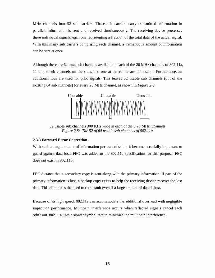
Although there are 64 total sub channels available in each of the 20 MHz channels of 802.11a,

11 of the sub channels on the sides and one at the center are not usable. Furthermore, an

additional four are used for pilot signals. This leaves 52 usable sub channels (out of the

existing 64 sub channels) for every 20 MHz channel, as shown in Figure 2.8.

52 usable sub channels 300 KHz wide in each of the 8 20 MHz ChannelsFigure 2.8: The 52 of 64 usable sub channels of 802.11a

2.3.3 Forward Error Correction

With such a large amount of information per transmission, it becomes crucially important to

guard against data loss. FEC was added to the 802.11a specification for this purpose. FEC

does not exist in 802.11b.

FEC dictates that a secondary copy is sent along with the primary information. If part of the

primary information is lost, a backup copy exists to help the receiving device recover the lost

data. This eliminates the need to retransmit even if a large amount of data is lost.

Because of its high speed, 802.11a can accommodate the additional overhead with negligible

impact on performance. Multipath interference occurs when reflected signals cancel each

other out. 802.11a uses a slower symbol rate to minimize the multipath interference.

Unusable UnusableUnusable

14

Figure 2.9: The Effect of Multipath Signaling with Collisions

2.3.4 Multipath Reflection

Another threat to transmission integrity is Multipath reflection, also called delay spread.

When a radio signal leaves the sending antenna, it is radiates outward, spreading as it travels.

If the signal reflects off a flat surface, the original signal and the reflected signal may reach

the receiving antenna simultaneously. Depending on how the signals overlap, they can either

augment or cancel each other out.

A baseband processor, or equalizer, unravels the divergent signals. However, if the delay is

long enough, the delayed signal spreads into the next transmission. OFDM specifies a slower

symbol rate to reduce the chance a signal will encroach on the following signal, minimizing

multipath interference.

2.3.5 Data Rates and Ranges

Devices using 80.2.11a are required to support speeds of 6, 12, and 24 Mbps. Optional speeds

goes upto 54 Mbps, but will also typically include 48, 36, 18, and 9 Mbps. These differences

are the result of the implementation of different modulation techniques and FEC levels.

To achieve 54 Mbps, a mechanism called 64 QAM is used to peak the maximum amount of

information possible on each sub carrier. Similar to operation of 802.11b, as on 802.11a

client device travels farther from Access Point (AP), the connection will remain intact but the

speed decreases. As Figure 2.10 illustrates, 802.11a can have a significantly higher signaling

rate than 802.11b at most ranges.

Obstacle

Obstacle

X Signals Cancel eachother

Signal

15

Figure 2.10: A Comparison of transmission distances and speeds for 802.11a and 802.11b

2.3.6 The MAC Layer - 802.11a

802.11a uses the same MAC Layer technology as 802.11b. Carrier Sense Multiple Access

with Collision Avoidance (CSMA-CA). CSMA-CA is a basic protocol used to avoid the

signals colliding and canceling each other out. Signals using CSMA/CA request authorization

to transmit for a specific amount of time prior to sending information.

2.3.7 Four way Reliability Method Employed by 802.11a

The sending device broadcasts a request to send (RTS) frame with information regarding the

length of its signal. If the receiving device permits, it broadcasts a clear to send (CTS) frame.

Once the CTS frame goes out, the sending machine transmits its information. Any other

sending devices in the area that hear the CTS realize another device will be transmitting and

allow that signal to go out uncontested.

2.3.8 Compatibility and Inter Compatibility Features of 802.11a with 802.11b

While 802.11a and 802.11b share the same MAC layer technology, there are significant

differences at the physical layer. 802.11b, using the ISM band, transmits in the 2.4 GHz range,

while 802.11a, using the U-NII band, transmits in the 5 GHz range.

Because the 802.11a and 802.11b signals travel in different frequency bands, one significant

benefit to the user who happens to implement both within a building is that they will not

802.11a 802.11b

16

interface with each other. A related consequence, however, is that the two technologies are

not compatible, and people who employ 802.11a equipment can connect to users of 802.11b

equipment only through a wired backbone network that interconnects the two systems. There

are various strategies for migrating from 802.11b to 802.11a. Moreover, there are even hybrid

combination ‘ and ‘ APs and PC wireless cards for using both on the same network

concurrently. However, they increase the cost to the enterprise.

802.11a is not the next generation of enterprise class WLAN technology, although it has

many advantages over other current options. At speeds of 54 Mbps, it matches the 802.11g

protocol, and both ‘a’ version and ‘ version are faster than the ‘ version. 802.11a and

802.11b have similar range, but ‘a’ version provides higher speed than the ‘ version at each

spot throughput the entire coverage area.

Another advantage of the 802.11a that the 5 GHz band in which it operates is not highly

populated, so there is less congestion to cause interference or signal contention. And the eight

non overlapping channels of 802.11a allow for a highly scalable and flexible installation.

2.3.9 Transfer Rates and Distances of the Versions of 802.11

The maximum distance that 802.11 networks can transmit from the user station to an AP is

100 meters (or 330 feet). However, the speed achieved at this distance is only 2 Mbps. For

most data applications, 2 Mbps transmission is satisfactory. This transfer speed is equivalent

to that offered by the telephone company with its T1 private line and interoffice truncking

system. Also, distances less than 100 feet can achieve transfer speed upto 11 Mbps or even 54

Mbps (see Figure 2.11).

Figure 2.11: Various Speeds and Distances Achievable by 802.11 Networks

802.11

802.11a

802.11aExtensions

54M

8M

6M

4M

2MDistancein metersDate

Rate0 m 10 m 30 m 60 m 100 m

17

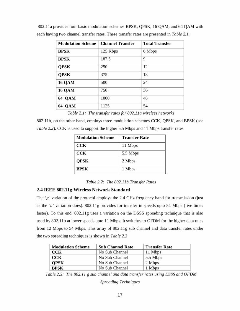
802.11a provides four basic modulation schemes BPSK, QPSK, 16 QAM, and 64 QAM with

each having two channel transfer rates. These transfer rates are presented in Table 2.1.

Table 2.1: The transfer rates for 802.11a wireless networks

802.11b, on the other hand, employs three modulation schemes CCK, QPSK, and BPSK (see

Table 2.2). CCK is used to support the higher 5.5 Mbps and 11 Mbps transfer rates.

Table 2.2: The 802.11b Transfer Rates

2.4 IEEE 802.11g Wireless Network StandardThe ‘ variation of the protocol employs the 2.4 GHz frequency band for transmission (just

as the ‘ variation does). 802.11g provides for transfer in speeds upto 54 Mbps (five times

faster). To this end, 802.11g uses a variation on the DSSS spreading technique that is also

used by 802.11b at lower speeds upto 11 Mbps. It switches to OFDM for the higher data rates

from 12 Mbps to 54 Mbps. This array of 802.11g sub channel and data transfer rates under

the two spreading techniques is shown in Table 2.3

Table 2.3: The 802.11 g sub channel and data transfer rates using DSSS and OFDM

Spreading Techniques

Modulation Scheme Channel Transfer Total Transfer

BPSK 125 Kbps 6 Mbps

BPSK 187.5 9

QPSK 250 12

QPSK 375 18

16 QAM 500 24

16 QAM 750 36

64 QAM 1000 48

64 QAM 1125 54

Modulation Scheme Transfer Rate

CCK 11 Mbps

CCK 5.5 Mbps

QPSK 2 Mbps

BPSK 1 Mbps

Modulation Scheme Sub Channel Rate Transfer RateCCK No Sub Channel 11 MbpsCCK No Sub Channel 5.5 MbpsQPSK No Sub Channel 2 MbpsBPSK No Sub Channel 1 Mbps

18

2.5 Comparing 802.11a, 802.11b, and 802.11g TechnologiesTable 2.4 presents the broad array of similarities and differences among the three current

802.11 WLAN approaches. A critical difference is that ‘a’ version operates at the less

congested bandwidth of 5 GHz, while the other two versions (b and g) operate at the lower

2.4 GHz bandwidth. On the other hand, the ‘ and ‘ versions are interoperable and can

operate at distances upto 124 meters (although normally the expected range is limited to 100

meters or 330 feet).

Table 2.4: Comparison of 802.11 a, b, and g versionsFrom a capacity standpoint, having more channels to carry traffic is a distinct advantage.

802.11a with its 12 or 24 channels (versus 802.11b and 802.11g with only 3 channels

available) provides a significantly larger capacity for carrying traffic. As an example, using a

common transfer rate in the lower range of 6 Mbps or 5.5 Mbps for the ‘ version, 802.11a

can carry 72 Mbps (6 Mbps times 12 channels) while the ‘ and ‘g‘ versions can only carry

about 18 Mbps. This advantage of 12 carrying channels can carry 608 Mbps while the g

version with only 3 channels can carry only 162 Mbps. Table 2.5 presents a comparison of

available capacity rates for the different protocols.

Table 2.5: Capacity Comparisons between the three (a, b, and g) 802.11 variations

802.11a 802.11b 802.11g

Frequency Band 5 GHz 2.4 GHz 2.4 GHz

Spread Type OFDM DSSS OFDM – FastDSSS – Slow

Transfer Speeds 54, 48, 36, 24, 12,9,6

11 Mbps OFDM54, 48, 36, 24,18DSSS11, 5.5, 2,1

Dist Range 54 Mbps - 13meters6 Mbps – 50meters

11 Mbps – 40meters1 Mbps – 124meters

54 Mbps – 27meters1 Mbps – 124meters

802.11a 802.11b 802.11g

Throughput

At Maximum

6 Mbps

54 Mbps

5.5 Mbps

11 Mbps

6 Mbps

54 Mbps# of ChannelsMixed Mode

12 3 3

Capacity – 6Mbps

72 Mbps 16.5 Mbps 18 Mbps

At MaxCapacity

648 Mbps 66 Mbps 162 Mbps

19

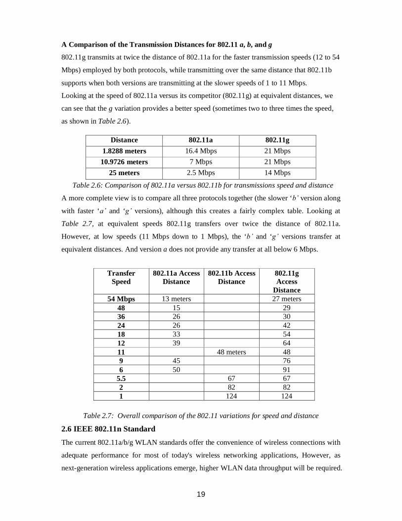
A Comparison of the Transmission Distances for 802.11 a, b, and g

802.11g transmits at twice the distance of 802.11a for the faster transmission speeds (12 to 54

Mbps) employed by both protocols, while transmitting over the same distance that 802.11b

supports when both versions are transmitting at the slower speeds of 1 to 11 Mbps.

Looking at the speed of 802.11a versus its competitor (802.11g) at equivalent distances, we

can see that the g variation provides a better speed (sometimes two to three times the speed,

as shown in Table 2.6).

Table 2.6: Comparison of 802.11a versus 802.11b for transmissions speed and distance

A more complete view is to compare all three protocols together (the slower ‘ version along

with faster ‘ and ‘ versions), although this creates a fairly complex table. Looking at

Table 2.7, at equivalent speeds 802.11g transfers over twice the distance of 802.11a.

However, at low speeds (11 Mbps down to 1 Mbps), the ‘ and ‘ versions transfer at

equivalent distances. And version a does not provide any transfer at all below 6 Mbps.

Table 2.7: Overall comparison of the 802.11 variations for speed and distance

2.6 IEEE 802.11n StandardThe current 802.11a/b/g WLAN standards offer the convenience of wireless connections with

adequate performance for most of today's wireless networking applications, However, as

next-generation wireless applications emerge, higher WLAN data throughput will be required.

Distance 802.11a 802.11g1.8288 meters 16.4 Mbps 21 Mbps

10.9726 meters 7 Mbps 21 Mbps25 meters 2.5 Mbps 14 Mbps

TransferSpeed

802.11a AccessDistance

802.11b AccessDistance

802.11gAccess

Distance54 Mbps 13 meters 27 meters

48 15 2936 26 3024 26 4218 33 5412 39 6411 48 meters 489 45 766 50 91

5.5 67 672 82 821 124 124

20

In response to this need, both IEEE TGn and the Wi-Fi Alliance have set expectations for the

next generation of WLAN standard 802.11n. The operating frequency of 802.11n is 2.4 GHz

and/or 5 GHz. It will use Multiple Input Multiple Output (MIMO) OFDM modulation

technique. The real data throughput will reach a theoretical 270 Mbit/s, and is up to 20 times

faster than 802.11b, and up to 3 times faster than 802.11a and up to 4 times faster than

802.11g. In addition, 802.11n will support all major platforms, including consumer

electronics, personal computing, and handheld platforms, and will be usable throughout all

major environments, including enterprise, home, and public hotspots.

802.11n builds upon previous 802.11 standards by adding MIMO. MIMO uses multiple

transmitter and receiver antennas to allow for increased data throughput via spatial

multiplexing and increased range by exploiting the spatial diversity. This is beyond the scope

of the thesis.

2.7 Chapter Conclusion

Given the data, it is rather obvious that the 802.11g specification is the current preferred

choice, providing high transfer speed and decent transmission distances. However, there has

been some resurgence in interest in version ‘ . Its carrying capacity and use of the 5 GHz

frequency range with low noise and competition is certainly an advantage. On the other hand,

the ‘ and ‘ versions are interoperable since they both use the 2.4 GHz frequency and the

same modulation and encoding processes at the lower transmission speed. However, they are

plagued with more interface, noise, and competition from other signaling systems. So there

will be some interest in the future in achieving version ‘g‘transmission distances at the 5 GHz

frequency.

21

Chapter 3MODULATION SCHEMES

22

3. Modulation Schemes

3.1 IntroductionIn communication, modulation is the process of varying a periodic waveform, in order to use

that signal to convey a message. Normally a high frequency waveform is used as a carrier

signal. The three key parameters of a sine wave are frequency, amplitude, and phase, all of

which can be modified in accordance with a low frequency information signal to obtain a

modulated signal.

The aim of digital modulation is to transfer a digital bit stream over an analog band pass

channel or a radio frequency band. The changes in the carrier signal are chosen from a finite

number of alternative symbols. Amplitude shift keying (ASK), frequency shift keying (FSK),

phase shift keying (PSK), QAM are the most fundamental digital modulation schemes. In

PSK and QAM, the modulation alphabet is conveniently represented on a constellation

diagram, showing the amplitude of inphase (I) component on x-axis and the amplitude of

Quadrature (Q) component on y-axis, for each symbol. ‘I’ and ‘Q’ signals can be combined

into a complex valued signal called the equivalent baseband signal. This is a representation of

the value modulated physical signal.

This chapter discusses the different modulation schemes used in OFDM. Following the

introduction; Section 3.2 describes the Phase Shift Keying modulation, Section 3.3 describes

Quadrature Amplitude Modulation, and Section 3.4 describes the conclusions and simulation

results.

3.2 Phase Shift Keying (PSK)PSK relies on carrier changing between distinct phases of the signal to define the status of

information being transmitted. PSK default is considered for binary (two) levels of phase

modulations. PSK is considered a very efficient process of data delivery because of low bit

error rates in the delivery. A number of variations of PSK are used in wireless networking

systems, among which are BPSK, QPSK. Most of current wireless systems employ some

form of PSK.

23

3.2.1 Binary Phase Shift Keying (BPSK)

In BPSK, the phase of the carrier signal is switched depending upon whether the source data

from the user is a zero or a one. As an example, in Figure 3.1 & 3.2, the signal is changing

phase in the transition bits from 0 to 1 and from 1 to 0. There is no phase change for the

continuity of the same bit pattern.

Figure 3.1: Change of phase with symbol change

Following the standard modulation process, the user’s source data is modulated against the

carrier signal centered on the frequency band.

Figure 3.2: Phase Shift Modulation Process

1 0 1 1

Change of Phase

Phase ShiftKeyingModulation

Source DigitalSignal

1 0 1 1

Phase Shifts

Resultant Carrier Signal Modulated by theSource SignalCarrier Signal + Source

Signal Modulation

24

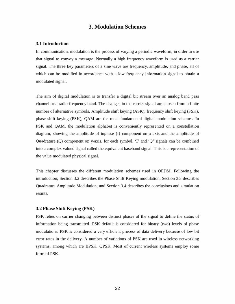
With BPSK process, modulated wave shifts between two phase phases, which are 180

degrees apart. The zero and the one are represented by the 0 degree and the 180 degree

phases. A phase diagram showing those two phases is shown in Figure 3.3

Figure 3.3: A Phase diagram showing the 0 and 180 degree phases

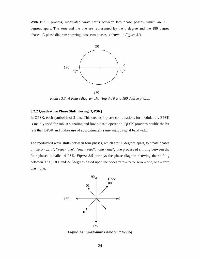
3.2.2 Quadrature Phase Shift Keying (QPSK)

In QPSK, each symbol is of 2-bits. This creates 4-phase combinations for modulation. BPSK

is mainly used for robust signaling and low bit rate operation. QPSK provides double the bit

rate than BPSK and makes use of approximately same analog signal bandwidth.

The modulated wave shifts between four phases, which are 90 degrees apart, to create phases

of “zero - zero”, “zero - one”, “one - zero”, “one - one”. The process of shifting between the

four phases is called 4 PSK. Figure 3.5 portrays the phase diagram showing the shifting

between 0, 90, 180, and 270 degrees based upon the codes zero – zero, zero – one, one – zero,

one – one.

Figure 3.4: Quadrature Phase Shift Keying

0180

90

270

“1” “0”

Code0001

10

180degrees

90

0degrees

270degrees

11

25

3.3 Quadrature Amplitude Modulation (QAM)For higher data rates, PSK has limitations. QAM provides the higher throughput rate required

for data transfers by combining ASK and PSK. Two different signals are sent simultaneously

on the same carrier frequency. The result of this combination provides two variable

(amplitude and phase of the signal) to assign binary values. As the number of states are

increasing, greater throughput is achieved. The number of states used in QAM ranges from 8

to 4096 in practical systems making data throughput to 100 Mbps rate in WLAN and very

high speed digital subscriber line (VHDSL) systems.

The diagram in Figure 3.5 & 3.6 represents the four quadrants of possible phase change and

four groups of symbols or possible data combinations that can be delivered with the varying

amplitude and phase shifts of the signal. As the complexity of QAM increases, the possibility

of data loss also increases.

Figure 3.5: Constellation Diagrams for 16 QAM

Figure 3.6: Constellation Diagrams for 64 QAM

26

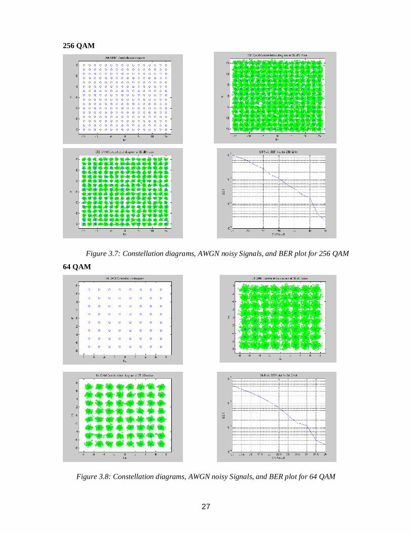
3.4 Simulations of QAMM-QAM has been simulated in Matlab. M used in the simulation is 4, 16, 64, and 256.

Different QAM results summary is given in the Table 3.1. The results are compared for BER

of 10-3. For 4 QAM the SNR is approximately 10.5 dB, for 16 QAM the SNR is

approximately 17.5 dB, for 64 QAM the SNR is approximately 24.2 dB, and for 256 QAM

the SNR is approximately 30.2 dB. As the M value increases in order to maintain good BER,

SNR also needs to be increased appropriately. For each QAM points, separate Figures are

given.

• Figure 3.7 is for 256 QAM. In this figure, basic constellation, decoded constellations for

two different SNRs and BER is plotted for different SNRs.







Modulation SNR in dB

4 QAM 10.5

16 QAM 17.5

64 QAM 24.2

256 QAM 30.2

Table 3.1: SNR comparison over AWGN channel for different QAM modulations at BER of 10-3

27

256 QAM

Figure 3.7: Constellation diagrams, AWGN noisy Signals, and BER plot for 256 QAM

64 QAM


28

16 QAM


4 QAM

Figure 3.10: Constellation diagram, AWGN noisy signals, and BER plot for 4 QAM

29

3.5 Chapter ConclusionIn wireless systems PSK and QAM modulations are popularly used. In general PSK and

QAM are used in several base band signal processing. PSK is mainly used for low bit rate

transmissions. PSK operates at low SNR or for the given link conditions, they give better

BER performance. Hence, PSK modulations are used for initial signaling, messages, and low

data rates.

QAM is most popular for higher data rates. Most popularly QAM is used from 16 to 1024.

Some base band signal processors are also using 4096 QAM. In QAM, the margins are low

between signal constellation points. Hence, any imbalances or impediments in the channel or

overall system can make the BER to grow. To contain BER low, it is required to send higher

power. In practical systems power is limited. Hence, QAM is used with error correction

schemes like FEC with RS codes. QAM used with MCM develop higher peak powers.

Sometimes, peak transmitted power is limited. This may develop more errors. Once again,

peak power clipping and error correction schemes help here.

30

Chapter 4ORTHOGONAL FREQUENCY DIVISION MULTIPLEXING

31

4. Orthogonal Frequency Division Multiplexing

4.1 IntroductionOFDM systems are better than single-carrier systems in multi-path fading channel

environment. OFDM is used in many high data rate transmission systems, for example, DVB,

IEEE 802.11, IEEE 802.16, HIPERLAN Type II, many derivatives of DSL and Home

networking etc. It is projected that OFDM systems are the strongest candidate for 4G systems.

OFDM is a digital carrier modulation scheme, which uses a large number of closely spaced

orthogonal sub carriers. Each sub carrier is modulated with a conventional modulation

scheme at low symbol rate, maintaining data rates similar to conventional single carrier

modulation schemes in the same bandwidth.

The primary advantage of OFDM over single carrier schemes is its ability to cope with severe

channel conditions like multipath, narrowband interference without complex equalization

filters. Channel equalization is simplified because OFDM may be viewed as using many

slowly modulated narrowband signals rather than one rapidly modulated wideband signal.

The orthogonality of the subcarriers results in zero cross talk, even though they are so close

that their spectra overlap. Low symbol rate helps manage time domain spreading of the signal

by allowing the use of guard interval between the symbols. The guard interval also eliminates

the pulse shaping filter.

This Chapter discusses the implementation and simulation of OFDM system in Matlab.

Following the introduction this chapter, Section 4.2 describes detailed description of OFDM,

Section 4.3 & 4.4 describe importance of Fourier Transform in OFDM, Section 4.5 describes

importance of Guard interval, Section 4.6 describes Choice of key elements used in OFDM,

and Section 4.7 is presented with simulation results.

32

4.2 Orthogonal Frequency Division Multiplexing4.2.1 The Importance of Orthogonality

The “orthogonal” part of the OFDM name indicates that there is a precise mathematical

relationship between the frequencies of the carriers in the system. Considering set of signals

pΨ , where pΨ is the p-th element in the set. The signals are orthogonal if

* k for p = q0 for p q( ) ( ) q

b

p

a

t t ≠Ψ Ψ =∫where the * indicates the complex conjugate and interval [a,b] is a symbol period. A fairly

simple mathematical proof exists, that the series sin(mx) for m=1,2,… is orthogonal over the

interval -π to π . Most of transform theory makes the use of orthogonal series.

Frequency division multiplexing (FDM) is used in many communication systems. In a

normal FDM system, the many carriers are spaced apart in such way that the signals can be

received using conventional filters and demodulators. In such receivers, guard bands have to

be introduced between the different carriers as shown in Figure 4.1. The introduction of these

guard bands in the frequency domain result in a lowering of the spectrum efficiency.

Figure 4.1: Functional bands representation of FDM and OFDM

It is possible, however, to arrange the carriers in an OFDM signal so that the sidebands of the

individual carriers overlap and the signals can still be received without adjacent carrier

interference. In order to do this all the carriers must be mathematically orthogonal in a

symbol interval. The receiver acts as a bank of demodulators, translating each carrier down to

DC, the resulting signal then being integrated over a symbol period to recover the raw data. If

Conventional FDM multicarrier modulation technique

OFDM multicarrier modulation technique

33

the other carriers all beat down to frequencies which, in the time domain, have a whole

number of cycles in the symbol period (τ ), then the integration process results in zero

contribution from all these carriers. Thus the carriers are linearly independent (i.e.,

orthogonal) if the carrier spacing is a multiple of 1/τ .

4.2.2 Mathematical Description of OFDM

OFDM transmits a large number of narrowband carriers, closely spaced in the frequency

domain. In order to avoid a large number of modulators and filters at the transmitter and

complementary filters and demodulators at the receiver, it is desirable to be able to use

modern digital signal processing techniques, such as fast Fourier transform (FFT).

Mathematically, each carrier can be described as a complex wave

[ ]( )( ) ( ) c cj t tc cS t A t e ω +Φ= (4.1)

The real signal is the real part of ( )cS t . Both ( )cA t and ( )c tΦ , the amplitude and phase of the

carrier, can vary on a symbol by symbol basis. The values of the parameters are constant over

the symbol duration period τ .

OFDM consists of many carriers. Thus the complex signals ( )sS t is represented by

1[( ( )]

0

1( ) ( ) n n

Nj t t

s nn

S t A t eN

ω−

+Φ

=

= ∑ (4.2)

Where

n o nω ω ω= + V

The above representation is for a continuous signal. If we consider the waveforms of each

component of the signal over one symbol period, then the variables Ac (t) and (t) take fixed

values, which depend on the frequency of that particular carrier, and so can be rewritten

( )( )

n n

n n

tA t AΦ ⇒ Φ

⇒

If the signal is sampled using a sampling frequency of 1/T, then the resulting signal is

represented by

0

1[( ) ]

0

1( ) n

Nj n kT

s nn

S kt A eN

ω ω−

+ +Φ

=

= ∑ V

(4.3)

At this point, we have restricted the time over which we analyze the signal to N samples. It is

convenient to sample over the period of one data symbol. Thus we have a relationship

34

NTτ =

If we now simplify Equation 4.3, without a loss of generality by letting 0=0, then the signal

becomes1

( )

0

1( ) n

Nj j n kT

s nn

S kt A e eN

ω−

Φ

=

= ∑ V

(4.4)

Now Equation 4.4 can be compared with the general form of the inverse Fourier transform1

2 /

0

1( ) ( )N

j nk Ns

n

ng kt G eN NT

π−

=

= ∑ (4.5)

In Equations 4.4, the function njnA e Φ is no more than a definition of the signal in the sampled

frequency domain, and s(kT) is the time domain representation. Equations 4.4 and 4.5 are

equivalent if

1 12

fNT

ωπ τ

= = =V

V (4.6)

This is the same condition that was required for orthogonality (see Importance of

orthogonality). Thus, one consequence of maintaining orthogonality is that the OFDM signal

can be defined by using Fourier transform procedures.

4.3 The Fourier TransformThe Fourier transform allows transformation from time domain to frequency domain.

The conventional Fourier transform relates to continuous signals which are not limited to in

either time or frequency domains. However, signal processing is made easier if the signals are

sampled. Sampling of signals with an infinite spectrum leads to aliasing, and the processing

of signals which are not time limited can lead to problems with storage space.

To avoid this, the majority of signal processing uses a version of the DFT. The DFT is a

variant on the normal transform in which the signals are sampled in both time and the

frequency domains. By definition, the time waveform must repeat continually, and this leads

to a frequency spectrum that repeats continually in the frequency domain.

FFT is merely a rapid mathematical method for computer applications of DFT. It is the

availability of this technique, and the technology that allows it to be implemented on

integrated circuits at a reasonable price, that has permitted OFDM to be developed as far as it

has. The process of transforming from the time domain representation to the frequency

35

domain representation uses the Fourier transform itself, whereas the reverse process uses the

inverse Fourier transform.

4.4 Signal Representation of OFDM using IFFT/FFTThe definition of the N-point DFT is

[ ]1

(2 / )

0[ ]

Nj N kn

p pn

X k x n e π−

−

=

= ∑ (DFT) (4.7)

And the N-point IDFT is

[ ]1

(2 / )

0

1 [ ]N

j N knp p

kx n X k e

Nπ

−

=

= ∑ (IDFT) (4.8)

A natural consequence of this method is that it allows us to generate carriers that are

orthogonal. The members of an orthogonal set are linearly independent.

Consider a data sequence (d0, d1, d2, …, dN-1), where each dn is a complex number dn=an+jbn.

(an, bn= ± 1 for QPSK, an, bn= ± 1, ± 3 for 16-QAM, an, bn = ± 1, ± 3, ± 5 for 64 QAM, and

an, bn= ± 1, ± 3, ± 5, ± 7 for 256 QAM)

1 12(2 / )

0 0

n m

N Nj f tj nm N

m n nn n

D d e d e ππ− −

−−

= =

= =∑ ∑ k = 0, 1, 2, 3…..N-1 (4.9)

where /( )nf n N T= V , kt k t= V and tV is an arbitrarily chosen symbol duration of the serial

data sequence dn.

The real part of the vector D has components

1

0Re [ cos(2 ) sin(2 )]

N

m m n n m n n mn

Y D a f t b f tπ π−

=

= = +∑ , k = 0, 1, 2, 3…..N-1

(4.10)

If these components are applied to a low-pass filter at time intervals tV , a signal is obtained

that closely approximates the frequency division multiplexed signal1

0( ) [ cos(2 ) sin(2 )],0

N

n n m n n mn

y t a f t b f t t N tπ π−

=

= + ≤ ≤∑ V (4.11)

36

Figure 4.2: Block diagram of an OFDM system using FFT

Figure 4.2 illustrates the process of a typical FFT-based OFDM system. The incoming serial

data is first converted form serial to parallel and grouped into ‘x’ bits each to form a complex

number. The number ‘x’ determines the signal constellation of the corresponding subcarrier,

such as BPSK, QPSK, 16 QAM, 64QAM, and 256 QAM. The complex numbers are

modulated in the baseband by the inverse FFT (IFFT) and converted back to serial data for

transmission. The receiver performs the inverse process of the transmitter. The Figure 4.2 on

base band OFDM functions. Complete system is not shown in this Figure 4.2.

Figure 4.3: Examples of OFDM spectrum (a) a single subchannel, (b) 5 carriers at the

central frequency of each subchannel, there is no crosstalk from other subchannels

Figure 4.3a shows the spectrum of an OFDM subchannel and Figure 4.3b shows an OFDM

spectrum. By carefully selecting the carrier spacing, the OFDM signal spectrum can be made

flat and the orthogonality among the subchannels can be guaranteed

Serial datainput Serial to

ParallelConverter

SignalMapping

Guard bitinsertioncircuit

IFFT

FFTRemovalof Guardinterval

Signaldemapper

Parallel toSerialConverter

Serial dataoutput

A Spectrum of OFDM Subchannel OFDM Spectrum

37

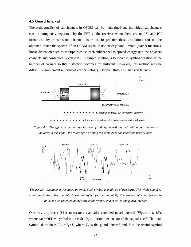
4.5 Guard IntervalThe orthogonality of subchannels in OFDM can be maintained and individual subchannels

can be completely separated by the FFT at the receiver when there are no ISI and ICI

introduced by transmission channel distortion. In practice these conditions can not be

obtained. Since the spectra of an OFDM signal is not strictly band limited (sinc(f) function),

linear distortion such as multipath cause each subchannel to spread energy into the adjacent

channels and consequently cause ISI. A simple solution is to increase symbol duration or the

number of carriers so that distortion becomes insignificant. However, this method may be

difficult to implement in terms of carrier stability, Doppler shift, FFT size and latency.

Figure 4.4: The effect on the timing tolerance of adding a guard interval. With a guard interval

included in the signal, the tolerance on timing the samples is considerably more relaxed

Figure 4.5: Example of the guard interval. Each symbol is made up of two parts. The whole signal is

contained in the active symbol (shown highlighted for the symbol M). The last part of which (shown in

bold) is also repeated at the start of the symbol and is called the guard interval

One way to prevent ISI is to create a cyclically extended guard interval (Figure 4.4, 4.5),

where each OFDM symbol is preceded by a periodic extension of the signal itself. The total

symbol duration is Ttotal=Tg+T, where Tg is the guard interval and T is the useful symbol

38

duration. When the guard interval is longer than the channel impulse response, or the

multipath delay, the ISI can be eliminated. However, the ICI, or in-band fading, still exists.

The ratio of the guard interval to useful symbol duration is application-dependent. Since the

insertion of guard interval will reduce data throughput, Tg is usually less than T/4.

The Reasons to use a Cyclic Prefix for the Guard Interval are

1. To maintain the receiver carrier synchronization, some signals instead of a long silence

must always be transmitted.

2. Cyclic convolution can still be applied between the OFDM signal and the channel

response to model the transmission system.

4.6 Choice of the Key Elements4.6.1 Useful Symbol Duration

The useful symbol duration T affects the carrier spacing and coding latency. To maintain the

data throughput, longer useful symbol duration results in increase of the number of carriers

and the size of FFT (assuming the constellation is fixed). In practice, carrier offset and phase

stability may affect how close two carriers can be placed. If the application is for the mobile

reception, the carrier spacing must be large enough to make the Doppler shift negligible.

Generally, the useful symbol duration should be chosen so that the channel is stable for the

duration of a symbol.

4.6.2 Number of Carriers

The number of sub carriers can be determined based on the channel bandwidth, data

throughput and useful symbol duration.

1Nτ

=

The carriers are spaced by the reciprocal of the useful symbol duration. The number of

carriers corresponds to the number of complex points being processed in FFT. For IEEE

802.11 , WLAN applications, the number of sub carriers are 52 (48 data carriers plus 4

pilot carriers).

4.6.3 Modulation Scheme

The modulation scheme in an OFDM system can be selected based on the requirement of

power or spectrum efficiency. The type of modulation can be specified by the complex

39

number dn=an+jbn. The symbols an and bn can be selected to ( ± 1, ± 3, ± 5, ± 7) for 256

QAM, ( ± 1, ± 3, ± 5) for 64 QAM, ( ± 1, ± 3) for 16QAM and ± 1 for QPSK. In general, the

selection of the modulation scheme applying to each sub channel depends solely on the

compromise between the data rate requirement and transmission robustness. Another

advantage of OFDM is that different modulation schemes can be used on different

subchannels for layered services.

4.7 Advantages and Disadvantages of OFDMThe advantages of OFDM are

1. Efficient use of the available bandwidth since the subchannels are overlapping

2. Spreading out the frequency fading over many symbols. This effectively randomizes the

burst errors caused by the Rayleigh fading, so that instead of several adjacent symbols (in

time on a single-carrier) being completely destroyed, (many) symbols in parallel are only

slightly distorted.

3. The symbol period is increased and thus the sensitivity of the system to delay spread is

reduced.

The Disadvantages of OFDM are

1. OFDM signal is contaminated by non-linear distortion of transmitter power amplifier;

because it is a combined amplitude-frequency modulation (it is necessary to maintain

linearity)

2. OFDM is very sensitive to carrier frequency offset caused by the jitter of carrier wave and

Doppler Effect caused by moving of the mobile terminal.

3. At the receiver, it is very difficult to decide the starting time of the FFT symbol

4.8 Simulation ResultsTable 4.1 shows the configuration used for the simulations performed on OFDM signal. A 64

carrier system was used, FFT size of 64 is taken and QPSK, 16 QAM, 64 QAM, and 256

QAM modulation schemes are used. The OFDM signal is passed over AWGN channel and

the received signal is demodulated and compared with the original signal to calculate BER. It

is observed that for AWGN channel we have to maintain minimum of 10.5 dB for QPSK,

17.5 dB for 16 QAM, 24.2 dB for 64 QAM and 30.2 dB for 256 QAM at BER of 10-3. Figure

4.6 shows obtained simulations results for different modulation schemes in Matlab. It was

found that the SNR performance of OFDM is similar to a standard single carrier digital

40

transmission. This is to be expected, as the transmitted signal is similar to a standard

Frequency Division Multiplexing (FDM) system.

Table 4.1: OFDM System Parameters used for simulations

Figure 4.6: SNR v/s BER plots for OFDM system using subcarrier modulation schemes 256

QAM, 64 QAM, 16 QAM and QPSK

Parameter Value

Carrier Modulations Used QPSK, 16 QAM, 64 QAM, and 256

QAM

FFT Size 64

Number of Carriers 64

Channel AWGN

41

4.9 Chapter ConclusionOFDM is the most popular scheme now for higher bit rate applications. This has built in

orthogonality. This works based on simple frequency analysis. Spectrum utilization from

OFDM is much higher. Guard band protects from various interferences. Higher bandwidth

applications use up to 4096 QAM points. OFDM is easily implemented using fast

computation of FFT. Several OFDM based design use dedicated hardware for FFT. The other

names of Digital multi-tone (DMT) modulation, MCM are used in place of OFDM based

processing. OFDM is not sufficient for end to end applications. Several error correction,

interleaving schemes are used for better data throughput even under severe end to end

impediments.

42

Chapter 5REED SOLOMON CODED OFDM

43

5. Reed Solomon Coded OFDM

5.1 IntroductionOFDM has recently received increased attention due to its capability of supporting high data

rate communication in frequency selective fading environments which cause ISI. Instead of

using a complicated equalizer as in the conventional single carrier systems, the ISI in OFDM

can be eliminated by adding a guard interval which significantly simplifies the receiver

structure. However, in order to take advantage of the diversity provided by the multi-path

fading, appropriate frequency interleaving and coding is necessary. Therefore, coding

becomes an inseparable part in most OFDM applications and a considerable amount of

research has focused on optimum encoder and decoder design for information transmission

via OFDM over fading environments.

FEC is widely used in digital telecommunications systems to make it easier to encode and

decode signals. Coding (FEC techniques) introduces redundancy in data and adding delay.

Simplest error-detecting technique is parity check bit coding, i.e., adding an extra binary digit

at the end of each word. But it will be effective only if the probability of error is very low.

Coding allows us to reduce the information bit error rate while maintaining a fixed

transmission rate. In principle it allows us to reach Shannon’s limit with ingenious coding.

The RS block code is organized on the basis of groups of bits. Such groups of bits are

referred to as symbols. We store sequences of ‘m’ individual bits which appear serially in a

bit stream and thereafter operate with the m-bit sequence rather than individual bits. These

are called m-bit symbols. Even if an error occurs in a single bit of a symbol, the entire symbol

is in error. RS code has ‘k’ information symbols, ‘r’ parity symbols and a total codeword

length of ‘n’ (=k + r) symbols. The number of symbols in the codeword is arranged to be

n = 2m -1. The RS code is able to correct errors in‘t’ symbols where t=r/2.

This chapter discusses the performance of the OFDM with RS coding technique. Following

the introduction, Section 4.2 describes the encoding Section 4.3 describes about the decoding

techniques. Section 4.4 describes concluding remarks.

44

5.2 EncodingThe encoder is the easy bit. Since the code is systematic, the whole of the block can be read

into the encoder, and then output other side without alteration. Once the kth data symbol has

been read in, the parity symbol calculation is finished, and the parity symbols can be output

to give the full n symbols.

The idea of the parity words is to create a long polynomial (‘n’ coefficients long – it contains

the message and the parity) which can be divided exactly by the RS generator polynomial. At

the decoder, the received message block can be divided by the RS generator polynomial. If

the remainder of the division is zero, then no errors are detected. If there is a reminder, then

there are errors.

The encoder acts to divide the polynomial represented by the ‘k’ message symbols d(x) by

the RS generator polynomial g(x).

x(n-k)*d(x)/g(x) = q(x) + r(x)/g(x)

The term x(n-k) is a constant power of ‘x’, which is simply a shift upwards n-k places of all

the polynomial coefficients in d(x). The reminder after the division r(x) becomes the parity.

By concatenating the parity symbols on the end of ‘k’ message symbols, an ‘n’ coefficient

polynomial is created which is exactly divisible by g(x). The Figure 5.1 shows the Encoder.

Message

Encoded message

Generator Polynomial Reminder

Figure 5.1: Reed Solomon Encoder

5.3 DecodingDecoding is far harder task than encoding. Decode operation takes several stages. There

are plenty of sources available for software implementations of the various algorithms

required. The below block diagram (Figure5.2) shows the RS decoder. Each block is

explained in detail below.

ReminderCalculation Concataten

ation

45

r(x) m(x)

Figure 5.2: Reed Solomon Decoder

The major blocks in Reed Solomon decoder are

1. Syndrome Calculation

2. Error Polynomial Calculation

3. Error Location Calculation

4. Syndrome Calculation

5.3.1 Syndrome Calculation

Let the received polynomial be,

r(x) = r0 + r1x +r2x2 + ……. +rn-1xn-1 (5.1)

and the generator polynomial has roots , 2 3 ……. 2t, syndromes are calculated by

substituting these roots into received polynomial in Equation (5.1). Let the calculated

syndromes be S1, S2 … and S2t. From these Syndromes we will calculate error polynomial

using Berlekamp algorithm.

5.3.2 Error Polynomial Calculation using Berlekamp Algorithm

For calculating error polynomial we will use Berlekamp algorithm as explained below.

Algorithm

1) Initialize parameters i = 0, 0 = 1, u =0, (0)(x) = (-1)(x) = 1, L0 = 0.

2) i = i + 1.

3) Compute Si.

Li-1

4) i = Si + l(l -1) Sl-1

l =1

5) if i = 0 (i)(x) = (i-1)(x) and Li = Li-1 and go to step 9 else continue

6) (i)(x) = (i-1)(x) - i u(-1) x(i - u) (u-1)(x)

7) if Li-1 >= i - Li-1 then Li = Li-1 and goto step 9 else continue

8) u =i,and Li-1 = i - Li-1

ErrorLocations

SyndromeCalculation

SyndromeCalculation

ErrorPolynomialCalculation

BerlekampAlgorithm Chien

searchForneyAlgorithm

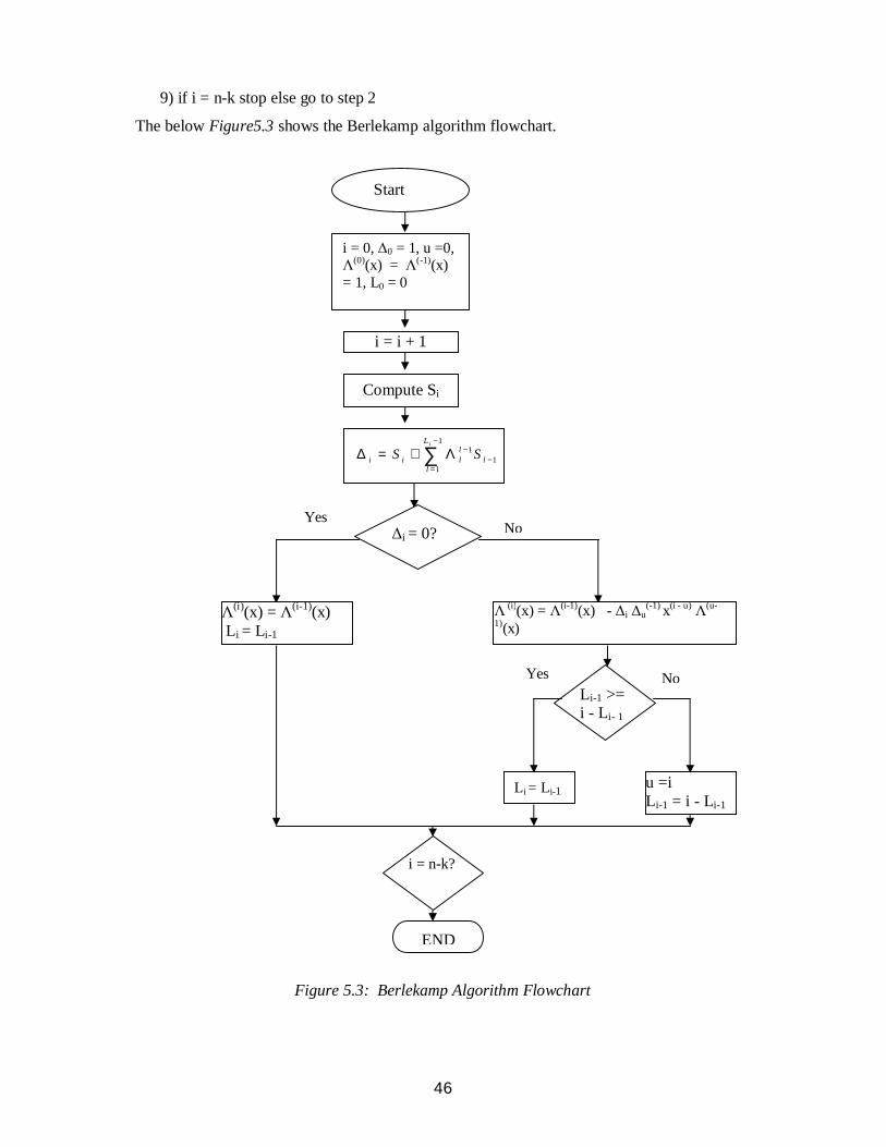
46

9) if i = n-k stop else go to step 2

The below Figure5.3 shows the Berlekamp algorithm flowchart.

Figure 5.3: Berlekamp Algorithm Flowchart

Start

i = 0, 0 = 1, u =0,(0)(x) = (-1)(x)

= 1, L0 = 0

i = i + 1

Compute Si

11

11

iLl

i i l ll

S S−

−−

=

∆ = + Λ∑

i = 0?

(i)(x) = (i-1)(x) Li = Li-1

(i)(x) = (i-1)(x) - i u(-1) x(i - u) (u-

1)(x)

Li-1 >=i - Li- 1

Li = Li-1 u =iLi-1 = i - Li-1

i = n-k?

END

YesNo

Yes No

47

5.3.3 Error Location Calculation using Chien Search

Let us denote error polynomial with2 3

1 2 3( ) 1 .... ttx x x x xΛ = + Λ + Λ + Λ + Λ

and we are interested in determining the roots of this polynomial since the polynomial is

defined over finite field, with primitive element then we show that if the order of field

is n, –i = n – i using this fact, if i is the root of the polynomial then we may write2 3

1 2 3( ) 1 ....i ttα α α α αΛ = + Λ + Λ + Λ + Λ

So the following steps, we may calculate the roots

1) For each power of in the range j = 0,1, …..n-1 use j as our test root

2) calculate the polynomial coefficients at the current root using, coefficients of the past

iteration using1 1j j i

i i α− −Λ = Λ during jth iteration

3) Calculate the polynomial coefficients, and if the sum1

0t

ji

i=Λ =∑

is equal to ‘0’ then save j as a root.

4) Continue to next iteration.

5.3.4 Error Magnitudes using Forney Algorithm

First, define an infinite-degree syndrome polynomial

2 2 2 11 2 2 2 1( ) ...... ....t t

t tS x S x S x S x S x ++= + + + +

Then, define the error magnitude polynomial as follows

( ) [1 ( )] ( )x S x xΩ = + Λ

Given that we know only the first 2t coefficients of S(x), the decoding problem becomes one

of finding a polynomial ( )xΛ of degree less than or equal to t that satisfies

2 1( )[1 ( )] ( ) mod tx S x x x +Λ + ≡ Ω

The error magnitudes are computed using the expression

1

1

( )( )k

k ki l

k

X XeX

−

−

− Ω=

Λ

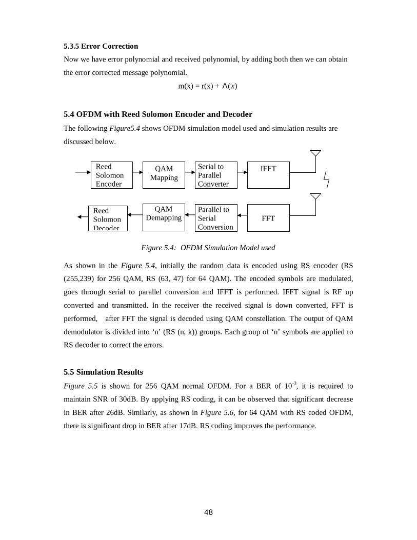
48

5.3.5 Error Correction

Now we have error polynomial and received polynomial, by adding both then we can obtain

the error corrected message polynomial.

m(x) = r(x) + ( )xΛ

5.4 OFDM with Reed Solomon Encoder and Decoder

The following Figure5.4 shows OFDM simulation model used and simulation results are

discussed below.

Figure 5.4: OFDM Simulation Model used

As shown in the Figure 5.4, initially the random data is encoded using RS encoder (RS

(255,239) for 256 QAM, RS (63, 47) for 64 QAM). The encoded symbols are modulated,

goes through serial to parallel conversion and IFFT is performed. IFFT signal is RF up

converted and transmitted. In the receiver the received signal is down converted, FFT is

performed, after FFT the signal is decoded using QAM constellation. The output of QAM

demodulator is divided into ‘n’ (RS (n, k)) groups. Each group of ‘n’ symbols are applied to

RS decoder to correct the errors.

5.5 Simulation ResultsFigure 5.5 is shown for 256 QAM normal OFDM. For a BER of 10-3, it is required to

maintain SNR of 30dB. By applying RS coding, it can be observed that significant decrease

in BER after 26dB. Similarly, as shown in Figure 5.6, for 64 QAM with RS coded OFDM,

there is significant drop in BER after 17dB. RS coding improves the performance.

ReedSolomonEncoder

QAMMapping

Serial toParallelConverter

IFFT

FFTParallel toSerialConversion

QAMDemapping

ReedSolomonDecoder

49

Figure 5.5: Comparison of OFDM and RS OFDM for 256 QAM

Figure 5.6: Comparison of OFDM and RS OFDM for 64 QAM

5.6 Chapter ConclusionFEC schemes are used along with modulation schemes like OFDM. RS is one of the popular

scheme. The RS codes are able to correct a corrupted symbol with a single bit error as it can

be symbol with all bits in error. RS used with OFDM improves the on BER that will result in

able to operate with lower SNR. This also helps in increase range. There are many other error

correction codes like Turbo codes that provide more gain than RS. From complexity and easy

VLSI implementation, RS is adapted popularly in base band processing.

50

Chapter 6ADAPTIVE CLIPPING TECHNIQUE FOR REDUCING PAPR ON

OFDM

51

6. Adaptive Clipping Technique for Reducing PAPR on OFDM

6.1 IntroductionThis chapter is concerned about PAPR reduction technique on OFDM systems. BER

performance of OFDM systems over clipping ratio (CR) are studied and simulated. We

considered adaptive clipping technique for PAPR reduction on OFDM systems by

modulation order.

This chapter discusses performance of the OFDM with PAPR technique. Following the

introduction, Section 6.2 describes PAPR problem, Section 6.3 describes System model used,

Section 6.4 describes about PAPR Reduction schemes, and Section 6.5 describes concluding

remarks.

6.2 PAPR Problem

OFDM systems have the undesirable feature of a large PAPR of the transmitted signals. The

transmitted signal has a non-constant envelope and exhibits peaks whose power strongly

exceeds the mean power. Consequently, to prevent distortion of the OFDM signal, the

transmit amplifier must operate in its linear regions. Therefore, power amplifiers with a large

dynamic range are required for OFDM systems - amplifiers which are prohibitively costly

and so continue to be the major cost component of OFDM systems. Consequently, reducing

the PAPR is pivotal to reducing the expense of OFDM systems.

6.3 System Model

Simplified baseband transmitter and receiver block diagram of OFDM systems, described at

Figure 6.1 are considered for analyzing a PAPR characteristics of OFDM signals. First,

transmitted binary source data is randomly generated. This random data is ‘1’ or ‘0’ and it

happens equally likely. Next, this random data is mapped through QAM constellation. QAM

mapped signal is complex value. Then, QAM mapped signal is loaded on each subcarrier,

and goes through serial to parallel conversion. And IFFT is performed. IFFT output signal is

operated with clipping for reducing PAPR, and then this signal is transmitted. The receiver

structure has reciprocal architecture to the transmitter.

52

Figure 6.1: OFDM Simulation Model

Analysis of OFDM Signal

IFFT output signal at Figure 6.1 is Equation 6.1.1

2 /

0

1( ) ( ) , 0,1, 2,... 1N

j kn N

kx n X k e n N

Nπ

−

=

= = −∑ (6.1)

N number of subcarriers

x (n) IFFT output signal, complex value

X (k) IFFT input signal, complex value

If the FFT size is N, then average power is 1/N and peak power is 1 regardless of N at IFFT

output side at Figure 6.1. So, PAPR equation can be written as Equation 6.2.

110log 10log1PAPR N

N

= = (6.2)

But peak power occurs very scarcely. Generally, the input signal of IFFT is a random data, so

the output signal of IFFT is a random data. If N is sufficiently large then statistical

characteristic of IFFT output signal is Gaussian random process by central limit theorem and

it can be written as from Equation 6.3 to Equation 6.5.2* ,

0, ( ) ( ) form nform nE x m x n σ =

≠= (6.3)

2 / 2,0, ( ) ( ) ( ) ( ) form n

R R I I form nE x m x n E x m x n σ =≠= = (6.4)

( ) ( ) 0R IE x m x n = (6.5)

x (n) R a real value of x(n)

x (n) I a imaginary value of x(n)

Now, we will tell a probability of peak power occurrence. When modulation is M-ary QAM

and IFFT size is N then number of occasions that input OFDM symbol can have is NM , and

peak power occurs 2M times. For example, N is 32 and QPSK modulation is used then

probability of peak power occurrence is 8.7 × 10-19. So this situation will never occur.

QAMMapping

Serial toParallelConversion

IFFT Clipping

FFTParallel toSerial

Conversion

QAMDemappingDecision

53

Therefore PAPR value is less important than probability distribution of IFFT output signal

power. Now we will consider probability of IFFT output signal power.

6.4 PAPR Reduction SchemesClipping, the simplest technique of PAPR reduction scheme, is operated by Equation 6.6.

2 22

2 2

( ), ( )( )

( ), ( )( )

A x n if x n Ax n

x n if x n Ay n

≤=

f

(6.6)2A is the maximum power

We define a CR to represent a clipping level. A CR is a ratio of the maximum power of

clipped signal over average power of unclipped signal. IFFT output signal is normalized, so

unclipped signal power is 1. If we clip a IFFT output signal at level A then a CR is 2A / 12A In this chapter we analyze probability distribution of IFFT output signal with FFT size

and modulation order and BER with the CR by computer simulation.

6.5 Simulation ResultsFigure 6.2 & 6.3 show BER performance with Modulation scheme and CR. In these figures

64-QAM and 256-QAM show an error flow phenomenon at CR. Table 6.1 shows a required

SNR when BER is 10-3 and we recommend a reasonable CR. When we use the 64 QAM

modulations, required SNRs when CR is 3 and 4 are shown, so we can use CR 4 when 64

QAM is used. Similarly for 256 QAM, required SNRs when CR is 4 and 5 are shown, so we

can use CR 5 when 256 QAM is used. So we propose the adaptive CR technique with

modulation order like Table 6.1. If we use this algorithm we can overcome PAPR problem of

OFDM systems with small BER degradation.

Table 6.1: Required SNR with Modulation and Clipping Ratio

64 QAM 256 QAM

Unclipped 24.2dB 30.2dB

CR = 5 -- 31dB

CR = 4 24.8dB > 35dB

CR = 3 > 30dB --

Recommended CR > 3 CR>4

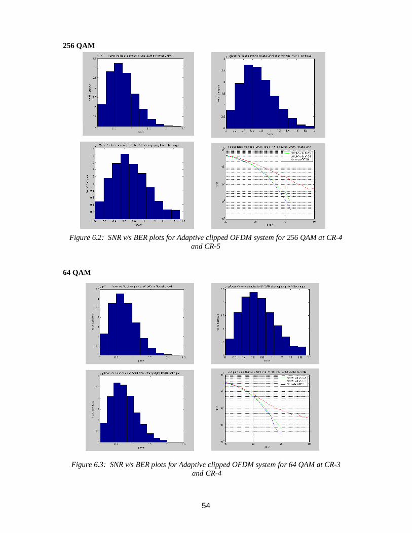
54

256 QAM

Figure 6.2: SNR v/s BER plots for Adaptive clipped OFDM system for 256 QAM at CR-4and CR-5

64 QAM

Figure 6.3: SNR v/s BER plots for Adaptive clipped OFDM system for 64 QAM at CR-3 and CR-4

55

6.5 Chapter ConclusionThe major drawback of OFDM system is when all the subcarriers are of same phase then the

instantaneous power is very high, this leads to nonlinear characteristics in amplifier.

To overcome this earlier techniques are First, clipping technique is used, but it has BER

degradation, second, peak power avoidance precoding technique, it will decreases the data

rate.

This proposed technique will be similar to clipping technique but it is adaptive to modulation

order. It is simple and combined advantages of both the clipping technique and peak power

precoding technique.

56

Chapter 7RS CODED OFDM FOR PAPR REDUCTION TECHNIQUE

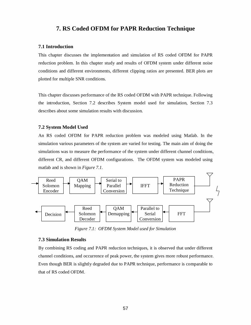
57

7. RS Coded OFDM for PAPR Reduction Technique

7.1 IntroductionThis chapter discusses the implementation and simulation of RS coded OFDM for PAPR

reduction problem. In this chapter study and results of OFDM system under different noise

conditions and different environments, different clipping ratios are presented. BER plots are

plotted for multiple SNR conditions.

This chapter discusses performance of the RS coded OFDM with PAPR technique. Following

the introduction, Section 7.2 describes System model used for simulation, Section 7.3

describes about some simulation results with discussion.

7.2 System Model UsedAn RS coded OFDM for PAPR reduction problem was modeled using Matlab. In the

simulation various parameters of the system are varied for testing. The main aim of doing the

simulations was to measure the performance of the system under different channel conditions,

different CR, and different OFDM configurations. The OFDM system was modeled using

matlab and is shown in Figure 7.1.

Figure 7.1: OFDM System Model used for Simulation

7.3 Simulation ResultsBy combining RS coding and PAPR reduction techniques, it is observed that under different

channel conditions, and occurrence of peak power, the system gives more robust performance.

Even though BER is slightly degraded due to PAPR technique, performance is comparable to

that of RS coded OFDM.

ReedSolomonEncoder

QAMMapping

Serial toParallel

ConversionIFFT

Decision

PAPRReductionTechnique

FFTParallel to

SerialConversion

QAMDemapping

ReedSolomonDecoder

58

Figure 7.2: Comparison of OFDM, RS coded OFDM, PAPR Reduced OFDM, and RS CodedOFDM for PAPR Technique for 256 QAM

Figure 7.3: Comparison of OFDM, RS coded OFDM, PAPR Reduced OFDM, and RS Coded

OFDM for PAPR Technique for 64 QAM

59

7.4 Chapter ConclusionOFDM is the most popular technique for high bit rates, but in wireless transmission there are

many parameters to consider for better performance. First, under severe channel conditions

decoding of the signal is a problem. To overcome this channel coding is necessary. Second,

OFDM has undesirable effect of occurrence of peak power which causes amplifier

characteristics non linear to overcome these peak power reduction techniques are necessary.

By combing RS coding, and Adaptive clipping techniques, the system behavior is robust to

channel conditions and peak power problem.

Considering from VLSI point of view, both RS coding and Adaptive clipping techniques are

simple and less complex for implementation, so recommended OFDM system is also robust

in terms of implementation.

60

Chapter 8CONCLUSION

61

8. Conclusion

8.1 Achievement of ThesisIn this thesis, various WLAN standards and the system aspects are presented at first level. We

then analyzed on multi carrier modulation scheme OFDM. Next, we have considered some of

the parameters which effect the wireless transmission of data through OFDM. We have

proposed a new system which is robust in terms of channel coding, peak power reduction,

and complexity. The main disadvantage of peak power of OFDM based systems can be

improved with PAPR techniques. This creates additional BER to the overall performance.

Error correction schemes like Reed-Solomon coding helps in both PAPR BER degradations

and also overall system performance. In this thesis, all the three techniques are combined for

overall better system performance. Several details and results of the techniques used are

presented in this thesis.

8.2 Scope of Further Research

Ø The proposed OFDM system is working well for AWGN channel, it can be tested to

Rayleigh fading channels.

Ø The proposed system can be applied at 60 GHz, which is current research area of

WLAN applications.

Ø The proposed system can be applied to MIMO OFDM, which is currently used in

IEEE WLAN 802.11n standard for higher data rates.

Ø Other coding techniques like Trellis, Convoltuional, and Turbo coding techniques can

be applied with adaptive clipping technique for PAPR reduction.

62

References

[1] R.W. Chang, “Synthesis of band- limited orthogonal signals for multichannel data

transmission,” Bell Sys. Tech. Journal, vol. 45, Dec. 1966

[2] William Y Zou, Yiyan Wu, “COFDM An Overview”, IEEE Transactions on

Broadcasting, vol 41, No.1, March 1995.

[3] Weinstein, S. and Ebert, P.; “Data Transmission by Frequency-Division Multiplexing

Using the Discrete Fourier Transform” IEEE Trans. on Commun. vol. 19, Issue: 5, pp. 628

–634, Oct.1971

[4] Peled, A. and Ruiz, A.; “Frequency domain data transmission using reduced

computational complexity algorithms”, Acoustics, Speech, and Signal Processing, IEEE

International Conference on ICASSP '80, vol. 5, pp.964 –967, Apr. 1980

[5] B. Hirosaki, “An analysis of automatic equalizers for orthogonally multiplexed QAM

systems,” IEEE Trans. Commun. , vol. COM-28, pp.73-83, Jan.1980.

[6] L.J. Cimini, “Analysis and simulation of a digital mobile channel using orthogonal

frequency division multiplexing”, IEEE Trans. Communications., vol. COM-33, pp. 665-

675. July 1985

[7] I. Kalet, “The multitone channel,” IEEE Trans. Commun. vol. 37, pp.119-124.

Feb.1989

[8] A.E. Jones, T.A. Wilkinson, and S.K. Barton, “Block coding scheme for reduction of

peak to mean envelope power ratio of multicarrier transmission schemes,” Electronics

Letters, vol. 30, no. 25, pp. 2098–2099, Dec 1994.

[9] J.A. Davis and J. Jedwab, “Peak-to-mean power control in ofdm, golay complementary

sequences, and reed-muller codes,” IEEE Trans. Inform. Theory, vol. 45, no. 7, pp. 2397 –

2417, Nov 1999.

[10] Geert Van Meerbergen, Marc Moonen, Hugo De Man, “Combining Rees- Solomon

Codes and OFDM for Impulse Noise Mitigation: RS-OFDM”, IEEE ICASSP 2006

Proceedings.

[11] Jun Tang, Xinyu Jin, Xianmin Zhang, Wenyu Cai, “A hybrid technique based on RS

coding and least square method for clipping distortion mitigation in OFDM system”, IEEE

Wi-COM 2006 Proceedings

[12] Yew Kuan Min and Varun Jeoti, “A Novel Signal Independent Technique for PAPR

Reduction in OFDM Systems” IEEE - ICSCN 2007, MIT Campus, Anna University,

Chennai, India. Feb. 22-24, 2007. pp.308-311.

63

[13] Hyung Jin Kim, Seong Chul Cho, Hyun Seo Oh, and Jae Min Ahn, “Adaptive Clipping

Technique for Reducing PAPR on OFDM System”, Proceedings of IEEE VTC 03, pp. 1478

-1481, 2003.

[14] Dustan Matiae, “OFDM as a possible modulation technique for multimedia applications

in the range of mm waves”, TUD-TVS, 1998.

[15] Zhengdao Wang, and Georgios B. Giannakis, “Wireless Multicarrier Communications

where Fourier meets Shannon”, IEEE Signal Processing Magazine, May 2000, pp., 29-48,

2000

[16] John A. C. Bingham, “Multi Carrier Modulation for Data Transmission An Idea Whose

Time Has Come”, IEEE Communications Magazine, pp., 5-14, 1990.

[17] Ramjee Prasad, and Luc Vandendorpe, “An Overview of Millimeter Wave Indoor

Wireless Communications Systems”, ICUPC, Conference, pp., 885-888, 1993.

[18] “Reed Solomon Encoder/Decoder IP Core”, Revision 1.4, February 2004, 4i2i

Communications Limited, 2004.

[19] Joel Sylvester, “Reed Solomon Codes”, Elektrobit, January 2001.

[20] Imdadul Islam, and Siddique Hossian, “Comparison of Traffic Performance of QPSK

and 16 QAM Modulation techniques for OFDM System”, Journal of Telecommunications

and Information Technology, pp., 147-152, 2005.

[21] “Orthogonal Frequency Division Multiplexing”, A Whitepaper by Intel

Communications, 2005.

[22] “Adaptive Modulation (QPSK, QAM)”, A Whitepaper by Intel Communications, 2004.

[23] William Carney, “IEEE 802.11g New Draft Standard Clarifies Future of Wireless LAN”,

A Whitepaper by Texas Instruments, 2002.

[24] Frank M. Groom, Kevin M. Groom, Stephen Jones, “The Basics of 802.11 Wireless

LANs”, IEC, 2005.

[25] Mohamed Ibnkaha, “Signal Processing for Mobile Communications Hand Book”, CRC

press, 2005.

[26] Xiaodong Wang, H. Vincent Poor, “Wireless Communications Systems Advanced

Techniques for Signal Reception”, Pearson Education, 2004.

[27] Paul Bedell, “Wireless Crash Course”, Tata McGraw Hill, 2002.

[28] T. S. Rappaport, “Wireless Communications Principles and Practice”, Pearson

Education, 2002.

[29] Robert H. Morelos, and Zaragoza, “The Art of Error Correcting Coding”, Wiley, 2002.

modeling and analysis of ofdm with adaptive...

Documents