modeling and analysis of hysteretic structural behavior
TRANSCRIPT
PB91-154195
CALIFORNIA INSTITUTE OF TECHNOLOGY
EARTHQUAKE ENGINEERING RESEARCH LABORATORY
MODELING AND ANALYSIS OFHYSTERETIC STRUCTURAL BEHAVIOR
By
Ravi Shanker Thyagarajan
Report No. EERL 89-03
A Report on Research Supported by Grantsfrom the National Science Foundation,
and by the Earthquake Research Affiliatesof the California Institute of Technology
Pasadena, California
1989
REPRODUCED BYu.S. DEPARTMENT OF COMMERCE
NATIONAL TECHNICALINFORMATION SERVICESPRINGFIELD, VA 22161
This investigation was sponsored by Grant Nos. CEE84-Q3780, CEE86-14906,
and CES88-15087 from the National Science Foundation and by the Earthquake
Research Affiliates of the California Institute of Technology under the supervision of
Wilfred D. Iwan. Any opinions, findings, conclusions or recommendations expressed
in this publication are those of the author and do not necessarily reflect the views
of the National Science Foundation.
f·
_II-w
502n-l01
REPORT DOCUMENTATION 11. REPORT NO.
PAGE EERL 89-034. Title and Subtitle
Modeling and Analysis of Hysteretic Structural Behavior
7. Author(s)
Ravi Shanker Thyagarajan9. Performing Organization Name and Addres.
California Institute of TechnologyMail Code 104-441201 E. California Blvd.Pasadena, California 91125
12. Sponsoring Organization Name and Address
National Science FoundationWashington, D.C. 20550
15. Supplementary Notes
3. Recipient'. Acces.lon No.
()B9J~j57liCJ55. Report Date
October 2, 1989
a. Performill8 O..enlzetlon Rept. No.
10. Proj8Ct/Tnk/Worlc Unit No.
11. Contract(C) or Grant(G) No.
(C) CEE84-03 780(G) CEE86-14906
CES88-l508713. Type of Report & Period Covered
14.
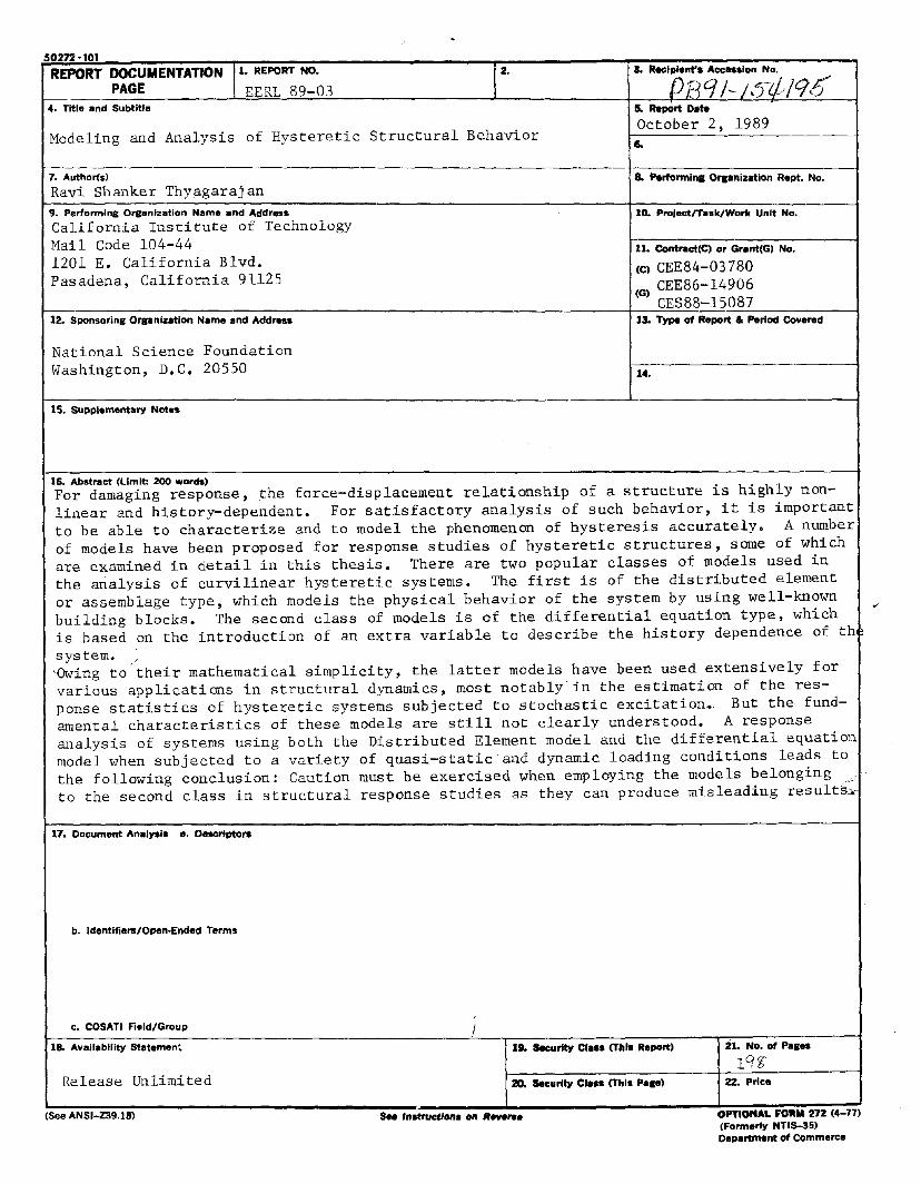
16. Abstract (limit: 200 words)For damaging response, the force-displacement relationship of a structure is highly non-linear and history-dependent. For satisfactory analysis of such behavior, it is importantto be able to characterize and to model the phenomenon of hysteresis accurately. A numberof models have been proposed for response studies of hysteretic structures, some of whichare examined in detail in this thesis. There are two popular classes of models used inthe analysis of curvilinear hysteretic systems. The first is of the distributed elementor assemblage type, which models the physical behavior of the system by using well-knownbuilding blocks. The second class of models is of the differential equation type, whichis based on the introduction of an extra variable to describe the history dependence of thsystem. /'Owing to their mathematical simplicity, the latter models have been used extensively forvarious applications in structural dynamics, most notably in the estimation of the response statistics of hysteretic systems subjected to stochastic excitation... But the fundamental characteristics of these models are still not clearly understood. A responseanalysis of systems using both the Distributed Element model and the differential equationmodel when subjected to a variety of quasi-static and dynamic loading conditions leads tothe following conclusion: Caution must be exercised when employing the models belongingto the second class in structural response studies as they can produce misleading results~
17. Document Analysi. a. Desc:rlptors
b. Identifiers/Open·Ended Terms
c. COSATI Field/Group
18. Availability Statemen,
Release Unlimited
(See ANSI-Z39.18)
I'. Security CI... (This Report)
20. security CI••• (Thl. P•••)
See '"lfruetlonl 0/1 Reverse
21. No. of Pages
1qg'22. Price
OPTIONAL FORM 272 (4-77)(Formerly NTI5-35)Department of Commerce

-I-Q..,~
MODELING AND ANALYSIS OF HYSTERETIC
STRUCTURAL BEHAVIOR
Thesis by
Ravi Shanker Thyagarajan
In Partial Fulfillment of the Requirements
for the Degree of
Doctor of Philosophy
California Institute of Technology
Pasadena, California
1990
(Submitted October 2, 1989)
-ii-
ACKNOWLEDGEMENTS
I am deeply grateful to Dr. Wilfred D. Iwan for his continued guidance, patience and
encouragement during the entire duration of my research. His infectious enthusiasm and his
ready availability to advise me with my work are very much appreciated.
I would like to thank the California Institute of Technology, Pasadena, for the fIrst
class education offered to me and for the generous fInancial support that made my graduate
study possible. The friendly environment that the staff, faculty and my student peers at
Thomas Lab offered is gratefUlly acknowledged, with special thanks to Donna and to
Cecilia, who also helped me with some of the illustrations in this thesis. I also wish to
express my gratitude to Dr. Thomas K. Caughey for the use of the CCO computers and to
Dr. James L. Beck for the very enjoyable educational experience I have had as his teaching
assistant.
My sincere thanks are due to Gupta, David, CVR, Truong, Jay, Todd and Katie for
the great times we have had together in the past five years and for their constant friendship.
My office-mate, Phalkun, deserves special thanks for all the things he has taught me. I
wish to offer heartfelt thanks to my friend and wife, Rama, for her love and for her
patience. Finally, I dedicate this thesis to my parents, Shrimati and Shri Palur R.
Thiagarajan, who gave up their dreams so that I could have mine, and for this I shall
remain forever in their debt.
-iii-
ABSTRACT
For damaging response, the force-displacement relationship of a structure is highly
nonlinear and history-dependent. For satisfactory analysis of such behavior, it is important
to be able to characterize and to model the phenomenon of hysteresis accurately. A number
of models have been proposed for response studies of hysteretic structures, some of which
are examined in detail in this thesis. There are two popular classes of models used in the
analysis of curvilinear hysteretic systems. The first is of the distributed element or
assemblage type, which models the physical behavior of the system by using well-known
building blocks. The second class of models is of the differential equation type, which is
based on the introduction of an extra variable to describe the history dependence of the
system.
Owing to their mathematical simplicity, the latter models have been used extensively
for various applications in structural dynamics, most notably in the estimation of the
response statistics of hysteretic systems subjected to stochastic excitation. But the
fundamental characteristics of these models are still not clearly understood. A response
analysis of systems using both the Distributed Element model and the differential equation
model when subjected to a variety of quasi-static and dynamic loading conditions leads to
the following conclusion: Caution must be exercised when employing the models
belonging to the second class in structural response studies as they can produce misleading
results.
The Massing's hypothesis, originally proposed for steady-state loading, can be
extended to general transient loading as well, leading to considerable simplification in the
the analysis of the Distributed Element models. A simple, nonparametric identification
technique is also outlined, by means of which an optimal model representation involving
one additional state variable is determined for hysteretic systems.
-IV-
TABLE OF CONTENTS
'tl .Tl e page 1
Acknowledgements ii
Abstract iii
Table of Contents iv
List of Tables and Figures vii
Chapter 1 IN"m.ODUCTION , 1
Chapter 2 MATIIEMATICAL MODELrnG OF HYSTERETIC BEHAVIOR 5
2.1 Introduction , 5
2.2 Piecewise-linear hysteretic (PLH) models 6
2.2.1 Introduction , 6
2.2.2 Elastoplastic and Bilinear models 7
2.2.3 Polylinear hysteretic model 8
2.2.4 The Clough-Johnston hysteretic modeL 9
2.2.5 Other piecewise-linear hysteretic models l0
2.3 Curvilinear hysteretic models 10
2.3.1 Massing's model. 10
2.3.2 The parallel-series (P-S) Distributed Element (DEL) model.. 11
2.3.3 The Extended Massing's hypothesis 16
2.3.4 Other DEL models satisfying the Extended
Massing's hypothesis 19
2.3.4.1 Two other parallel-series models 19
2.3.4.2 The series-parallel (S-P) model. '" 21
2.3.4.3 Stiffness- and strength- degrading model.. 23
2.3.5 Curvilinear models with one or two hidden state variables 25
2.3.5.1 The endochronic models 25
2.3.5.2 The Wen-Bouc and Casciyati models 26
2.4 The DEQ category of hysteretic models 28
2.5 A history-independent representation for a Distributed Element model.. 29
-y-
Chapter 3 AN IDENTIFICATION METIIOD FOR HYSTERETIC SYSTEMS .41
3.1 Introduction 41
3.2 The identification procedure 42
3.3 Identification examples 46
3.3.1 Example 1: The Wen-Bouc hysteretic system .46
3.3.2 Example 2: The Bilinear hysteretic system .48
3.3.3 Example 3: The Distributed Element hysteretic system .49
3.4 Conclusion 51
Chapter 4 COMPARATIVESTUDYOF1HEQUASI-STATIC
PERFORMANCE OF TWO HYSTERETIC MODELS 66
4.1 Introduction 66
4.2 Hysteretic model representations 67
4.3 Cyclic loading between fixed displacement limits 69
4.3.1 Symmetric cyclic loading 69
4.3.2 Asymmetric cyclic loading 72
4.4 Cyclic loading between fixed force limits 74
4.4.1 Symmetric cyclic loading 74
4.4.2 Asymmetric cyclic loading 76
4.5 The Drucker's and Ilyushin's postulates 80
4.6 Conclusion 82
Chapter 5 COMPARATIVE STUDY OF 1HE DYNAMIC PERFORMANCE
OF TWO HYSTERETIC MODELS 94
5.1 Introduction 94
5.2 Hysteretic model representations 95
5.3 Simple structural models 97
5.3.1 The Single-Degree-Of-Freedom (SDOF) system ~ 97
5.3.2 The Multi-Degree-Of-Freedom (MDOF) system 98
5.4 Time integration procedure 99
-vi-
5.5 Example 1: SDOF structure with a suddenly applied extemalload 101
5.5.1 Gravitational effects neglected 101
5.5.2 Gravitational effects included 104
5.6 Example 2: Structure subjected to earthquake excitation 106
5.6.1 SDOF system 106
5.6.2 MDOF system 110
5.7 Stochastic excitation 112
5.7.1 Introduction 112
5.7.2 Example 3: SDOF system with stationary white noise base
excitation 113
5.7.3 Example 4: Comparison of inelastic response spectra 120
5.7.4 A note on the maximum displacement prediction by
the two models 128
5.8 Conclusion 128
Chapter 6 SUMMARY AND CONCLUSIONS 164
REFERENCES 169
Figure 2.1:
Figure 2.2:
Figure 2.3:
Figure 2.4:
Figure 2.5:
Figure 2.6:
Figure 2.7:
Figure 2.8:
Figure 2.9:
Figure 3.1:
Figure 3.2:
Figure 3.3:
Figure 3.4:
Figure 3.5:
Figure 3.6:
Figure 3.7:
Figure 3.8:
-vii-
LIST OF TABLES AND FIGURES
The elastoplastic model (a) Restoring force characteristic (b) Schematic representation forthe system 32
Schematic representation for a system with a polylinear hysteretic characteristic 33
The Clough's hysteretic model for reinforced concrete structures (a) Restoring force behavior(b) The normalized hysteretic component, z 34
A typical hysteretic loop for steady-state system response 35
The parallel-series Distributed Element model for hysteresis 36
A loading sequence with nested loops subjected on the Distributed Element model.. ........ 37
The function y(f*) for (a) path 01 (b) path 12 (c) path 23 (d) path 34 (e) path 45 (t) path56 (g) path 67 of the loading sequence shown in Fig. 2.6 37-38
The series-parallel Distributed Element model (a) Schematic representation for the system(b) Restoring force characteristic 39
The restoring force behavior of a stiffness- and strength-degrading Distributed Elementmodel [13] 40
The identification base excitation at(t), which is a sinusoidal function with a linearlyincreasing amplitude 53
The verification base excitation a2(t), which is the N-S component of the 1940 El Centroearthquake 53
The displacement and velocity of the Wen-Bouc hysteretic system when subjected to theidentification excitation, ai (t) 54
The identification data for11 and the optimal polynomial fit for the data when the Wen-Bouchysteretic system is subjected to the identification excitation, ai (t) 55
The identification data forh and the optimal polynomial fit for the data when the Wen-Bouchysteretic system is subjected to the identification excitation, a1(t) 55
The displacement response of the Wen-Bouc hysteretic system and the correspondingoptimal model when subjected to the verification excitation, a2(t) 56
The velocity response of the Wen-Bouc hysteretic system and the corresponding optimalmodel when subjected to the verification excitation, a2(t) 56
The hysteretic restoring force diagram for (a) the Wen-Bouc hysteretic system (b) thecorresponding optimal model when each is subjected to the verification excitation, a2(t) ... 57
-viii-
Figure 3.9: The displacement and velocity of the bilinear hysteretic system when subjected to theidentification excitation. al (t) 58
Figure 3.10: The identification data for!I and the optimal polynomial fit for the data when the bilinearhysteretic system is subjected to the identification excitation. al (t) ...............•............... 59
Figure 3.11: The identification data for fz and the optimal polynomial fit for the data when the bilinearhysteretic system is subjected to the identification excitation. a1(t) 59
Figure 3.12: The displacement response of the bilinear hysteretic system and the corresponding optimalmodel when subjected to the verification excitation. a2(t) 60
Figure 3.13: The velocity response of the bilinear hysteretic system and the corresponding optimal modelwhen subjected to the verification excitation. a2(t) 60
Figure 3.14: The hysteretic restoring force diagram for (a) the bilinear hysteretic system (b) thecorresponding optimal model when each is subjected to the verification excitation. a2(t) ... 61
Figure 3.15: The displacement and velocity of the Distributed Element hysteretic system when subjectedto the identification excitation. al(t) 62
Figure 3.16: The identification data for !I and the optimal polynomial fit for the data when theDistributed Element hysteretic system is subjected to the identification excitation, al (t) ... 63
Figure 3.17: The identification data for fz and the optimal polynomial fit for the data when theDistributed Element hysteretic system is subjected to the identification excitation, al (t) ... 63
Figure 3.18: The displacement response of the Distributed Element hysteretic system and thecorresponding optimal model when subjected to the verification excitation. a2(t) 64
Figure 3.19: The velocity response of the Distributed Element hysteretic system and the correspondingoptimal model when subjected to the verification excitation. a2(t).•......•....................... 64
Figure 3.20: The hysteretic restoring force diagram for (a) the Distributed Element hysteretic system (b)the corresponding optimal model when each is subjected to the verification excitation, a2(t) ........................................................................................................................ 65
Figure 4.1: The hysteretic restoring force behavior of (a) the DEL model (b) the W-B model when cycledbetween fixed. symmetric displacement limits 84
Figure 4.2: Ratio of the energy dissipated by the W-B model to that dissipated by the DEL model forcyclic loading between fixed. symmetric displacement limits 85
Figure 4.3: The restoring force behavior of (a) the DEL model (b) the W-B model when cycled betweenfixed. asymmetric displacement limits. 1 and 1.5 86
Figure 4.4: The stable loops corresponding to the two hysteretic models when cycled between the fixed.asymmetric displacement limits. 2 and 4 87
Figure 4.5: The hys~eretic b:h~vior of the two models when subjected to cycling between fixed.symmetrIc force hmits 87
Figure 4.6: Ratio of the energy dissipated by the W-B model to that dissipated by the DEL model forcyclic loading between fixed. symmetric force limits 88
-IX-
Figure 4.7: The hysteretic behavior of (a) the DEL model (b) the W-B model when subjected to cyclingbetween fixed, asymmetric force limits : 89
Figure 4.8: The hysteretic behavior of the W-B model when subjected to one load cycle between fixed,asymmetric force limits 90
Figure 4.9: Three-dimensional plot of Idl, the absolute value of drift per nonzero mean cycle betweenthe fixed limits Zl and Z2 91
Figure 4.10: The behavior of the drift of the W-B model when subjected to one load cycle between fixed,asymmetric force limits 92
Figure 4.11: The hysteretic behavior of the Casciyati model when subjected to load cycles between fixed,asymmetric force limits 92
Figure 4.12: The Drucker's integral for (a) the Casciyati model (b) the W-B model when subjected to aload cycle in Z from Zl to Z2 and back to Zl. The value of Zl is 0.75 93
Table 5.1: Comparison of eight characteristic quantities in the response of the Wen-Bouc andDistributed Element models to the 1940 EI Centro earthquake 13Q
Table 5.2: System parameters for the cases for which comparison is made of the response statistics ofthe two models when subjected to white noise excitation. In all cases, the following werekept constant nominal natural frequency=lHz, viscous damping as a fraction of critical=5%,A=1.0 and the ratio /3/"1=-1.5• .............................................................................. 131
Table 5.3: Statistics of eight response quantities for the two hysteretic models subjected to white noisebase excitation for Case I listed in Table 5.2 132
Table 5.4: Statistics of eight response quantities for the two hysteretic models subjected to white noisebase excitation for Case II listed in Table 5.2 133
Table 5.5: Statistics of eight response quantities for the two hysteretic models subjected to white noisebase excitation for Case III listed in Table 5.2 134
Table 5.6: Statistics of eight response quantities for the two hysteretic models subjected to white noisebase excitation for Case IV listed in Table 5.2 135
Table 5.7: Statistics of eight response quantities for the two hysteretic models subjected to white noisebase excitation for Case V listed in Table 5.2 136
Table 5.8: Statistics of eight response quantities for the two hysteretic models subjected to white noisebase excitation for Case VI listed in Table 5.2 137
Figure 5.1: Schematic representation of a restoring force system 138
Figure 5.2: Initial loading curve for the hysteretic models 138
Figure 5.3: Model for a single-degree-of-freedom structure in a gravitational field subjected to anearthquake ground motion and a horizontal external force 139
Figure 5.4: Model for a multi-degree-of-freedom structure subjected to earthquake ground motion......139
Figure 5.5: The displacement response of the two hysteretic models when subjected to a sudden externalload. The post-yielding stiffness ratio is 0.05 and gravitational effects are neglected 140
-x-
Figure 5.6: The hysteretic restoring force-displacement diagrams for the two hysteretic models whensubjected to a sudden external load. The post-yielding stiffness ratio is 0.05 and gravitationaleffects are neglected 140
Figure 5.7: The velocity response of the two hysteretic models when subjected to a sudden extemalloadfor (a) the first 25 seconds after frrst application of the load (b) the next 50 seconds. Thepost-yielding stiffness ratio is 0.05 and gravitational effects are neglected. 141
Figure 5.8: The displacement response of the W-B model when subjected to a sudden extemalload fordifferent values of a, the post-yielding stiffness ratio 142
Figure 5.9: The displacement response of the two hysteretic models when subjected to a sudden externalload. The post-yielding stiffness ratio is 0.05 and gravitational effects are included(11=0.071) 142
Figure 5.10: The hysteretic restoring force-displacement diagrams for the two hysteretic models whensubjected to a sudden extemalload. The post-yielding stiffness ratio is 0.05 and gravitationaleffects are included (11=0.071) 143
Figure 5.11: The displacement response of the two hysteretic models when subjected to a sudden externalload. The post-yielding stiffness ratio is 0.05 and gravitational effects are included(11=0.250) 143
Figure 5.12: The hysteretic restoring force-displacement diagrams for the two hysteretic models whensubjected to a sudden external load. The post-yielding stiffness ratio is 0.05 and gravitationaleffects are included (11=0.250) 144
Figure 5.13: The N-S component of the 1940 El Centro earthquake l44
Figure 5.14: The hysteretic restoring force-displacement behavior of the (a) W-B model (b) DEL modelwhen subjected to the EI Centro earthquake 145
Figure 5.15: The displacement response of the two hysteretic models when subjected to the El Centroearthquake 146
Figure 5.16: The hysteretic restoring force response time history of the two models when subjected to theEl Centro earthquake 146
Figure 5.17: The velocity response of the two models when subjected to the El Centro earthquake..... 147
Figure 5.18: The maximum relative displacement, U"" of the two models when subjected to the El
Centro earthquake, for a range of yield levels 147
Figure 5.19: The ductility factor, fJ., of the two models when subjected to the El Centro earthquake, for arange of yield levels 148
Figure 5.20: The dynamic amplitude, (umax - Umin), of the two models when subjected to the El Centro
earthquake, for a range of yield levels 149
Figure 5.21: The maximum relative velocity, Um , of the two models when subjected to the El Centro
earthquake, for a range of yield levels 149
-xi-
Figure 5.22: The base shear coefficient, Cb , of the two models when subjected to the El Centro
earthquake, for a range of yield levels 149
Figure 5.23: The instant in time at which um occurs, tmax ' of the two models when subjected to the EI
Centro earthquake, for a range of yield levels 150
Figure 5.24: The final offset, uoff ' of the two models when subjected to the EI Centro earthquake, for a
range of yield levels 150
Figure 5.25: The hysteretic energy dissipated, E(I), by the two models when subjected to the EI Centroearthquake, for a range of yield levels 151
Figure 5.26: A two-story building structure subjected to earthquake ground motion 151
Figure 5.27: The displac~mentresponse of the first story of a two-story structure for the two modelswhen subjected to the EI Centro earthquake 152
Figure 5.28: The displacement response of the second story of a two-story structure for the two modelswhen subjected to the El Centro earthquake 152
Figure 5.29: The hysteretic restoring force-displacement behavior of the first story of a two-storystructure for (a) the W-B model (b) the DEL model when subjected to the EI Centroearthquake 153
Figure 5.30: The maximum relative displacement, Um ' of the two models when subjected to white noise
base excitation, for a range of yield levels. The three curves shown for each modelcorrespond to values of the mean minus one standard deviation, the mean, and the mean plusone standard deviation 154
Figure 5.31: The ductility factor, f.l, of the two models when subjected to white noise base excitation,for a range of yield levels. The three curves shown for each model correspond to the valuesof the mean minus one standard deviation, the mean, and the mean plus one standarddeviation 154
Figure 5.32: The maximum relative velocity, Um , of the two models when subjected to white noise base
excitation, for a range of yield levels. The three curves shown for each model correspond tothe values of the mean minus one standard deviation, the mean, and the mean plus onestandard deviation 155
Figure 5.33: The base shear coefficient, Cb , of the two models when subjected to white noise base
excitation, for a range of yield levels. The three curves shown for each model correspond tothe values of the mean minus one standard deviation, the mean, and the mean plus onestandard deviation 155
Figure 5.34: The final offset, Uoff ' of the two models when subjected to white noise base excitation, for
a range of yield levels. The three curves shown for each model correspond to the values ofthe mean minus one standard deviation, the mean, and the mean plus one standarddeviation 156
-xii-
Figure 5.35: The hysteretic energy dissipated, E(n, by the two models when subjected to white noisebase excitation, for a range of yield levels. The three curves shown for each modelcorrespond to the values of the mean minus one standard deviation, the mean, and the meanplus one standard.deviation 156
Figure 5.36: The probability density function of u"" the maximum relative displacement of the twomodels for Case III listed in Table 5.2 157
Figure 5.37: The probability density function of the normalized value of u"'. the maximum relativedisplacement of the two models for Case III listed in Table 5.2 157
Figure 5.38: The cumulative probability function of U",. the maximum relative displacement of the twomodels for Case III listed in Table 5.2 158
Figure 5.39: The probability density function of U"" the maximum relative velocity of the two modelsfor Case III listed in Table 5.2 158
Figure 5.40: The probability density function of Cb , the base shear coefficient of the two models forCase III listed in Table 5.2 159
Figure 5.41: The probability density function of uoff ' the final offset of the two models for Case III
listed in Table 5.2 159
Figure 5.42: The NRC Reg. Guide 1.60 Horizontal mean design response spectrum for a viscousdamping ratio of 2% 160
Figure 5.43: Envelope function used to modulate stationary, Gaussian noise to obtain earthquake-likeexcitations 160
Figure 5.44: The inelastic pseudovelocity (PSV) response spectrum of the two hysteretic modelscorresponding to the Reg. Guide 1.60 elastic spectrum shown in Fig. 5.42. These spectracorrespond to a mean value of about 4 in the response of the DEL mode!.. 161
Figure 5.45: The inelastic spectral velocity (SV) response spectrum of the two hysteretic modelscorresponding to the Reg. Guide 1.60 elastic spectrum shown in Fig. 5.42. These spectracorrespond to a mean value of about 4 in the response of the DEL mode!.. 161
Figure 5.46: The inelastic spectral acceleration (SA) response spectrum of the two hysteretic modelscorresponding to the Reg. Guide 1.60 elastic spectrum shown in Fig. 5.42. These spectracorrespond to a mean value of about 4 in the response of the DEL model.. 162
Figure 5.47: Comparison of the design base shear coefficient as per the elastic NRC spectrum, the DELmodel, the W-B model and the ATC-3.06lateral force procedure 162
Figure 5.48: Comparison of design displacement drifts as per the two hysteretic models and the ATC-3.06 code 163
-1-
CHAPTER 1
INTRODUCTION
Most structures respond inelastically when subjected to strong seismic excitations.
Not only is the restoring force behavior of such structures highly nonlinear, it also depends
on the previous history of the response. This history-dependence phenomenon is referred
to as Hysteresis, the study of which has attracted considerable attention from researchers in
earthquake engineering.
Previous research on the earthquake records of severely shaken buildings by Iemura
and Jennings [19], Beck [8] and McVerry [32] has clearly indicated that the response
behavior of the structures is markedly nonlinear, the conclusion of all the researchers being
that the use of linear models is sufficient to reproduce the actual behavior of the structures
only up to the onset of damage.
Several mathematical models have been proposed to describe the hysteretic behavior
of structures excited beyond the elastic range [10,13,14,20,24,47,49,54], some of which
are examined in detail in this thesis. These range from the simple elastoplastic model to the
very sophisticated Takeda's model. The reason for the surfeit of models is that no single
model has proven entirely satisfactory for the analysis of hysteretic systems for one reason
or another. For instance, the elastoplastic model is often felt to be too simple to yield good
approximations of actual systems when tested against experimental data, while the
Takeda's model is so complex that there are numerous cumbersome rules to be followed,
depending on the loading regime.
Since earthquakes are usually modeled by a stochastic excitation, the theory of
random vibration is often employed in conjunction with the theory of equivalent
linearization in order to obtain approximate response statistics of nonlinear systems
-2-
subjected to earthquake excitation. Initially, such a technique was successfully used for
nonhysteretic nonlinear systems. Recently, it has been extended to some piecewise-linear
hysteretic systems [3,36,47] with the help of representations provided by Asano and Iwan
[3], and Suzuki and Minai [47], which have helped cast the systems in-a purely history
independent framework involving an expanded set of state variables. Unfortunately, there
are only a few physically motivated hysteretic systems for which such representations are
available, basically being restricted to systems with a piecewise linear hysteretic
characteristic.
Most experimentally observed hysteresis loops [39] suggest that the transition from
the linear or elastic range into the yielding range of the deformation is not abrupt as
modeled by piecewise-linear models, but rather is quite smooth. There are two classes of
models that exhibit curved or rounded hysteresis loops, which are described in further
detail in the following two paragraphs.
The first class ofmodels is physically motivated. A very large number of elastoplastic
elements are combined in a certain way so as to provide curvilinear hysteretic behavior.
One such model for hysteresis has been used by Iwan [20] to determine the steady-state
dynamic response of a softening system subjected to trigonometric excitation and also to
compare steady-state results predicted by the model with experimental results from an
actual structure, namely, a single-story structure having structural steel columns. The
ability of these models to adequately represent the nonlinear behavior of an actual steel
structure is also demonstrated in [24]. Thus, these models can not only be constructed from
simple, well-understood physical building blocks, but they are also quite well suited for the
hysteretic modeling of actual steel structures.
In the second class of models, a finite number of additional state variables (usually
one or two) are introduced in the mathematical formulation to describe hysteretic behavior,
with each new state variable itself satisfying a first-order, single-valued, nonlinear ordinary
-3-
differential equation. Typical examples of such models are (i) the model originally
proposed by Bouc and later generalized by Wen [54], (ii) Casciyati's model [10], (iii)
Ozdemir's model [35], etc. Even though such models have been used for various
applications in structural dynamics, it is in the response analysis of hysteretic syst,
the method of equivalent linearization that they have been most widely applied. The i
belonging to this class have also been referred to in this thesis as endochronic I
because of the similarity in the quasi-static response behavior of these and
endochronic models [7,50] employed in plasticity.
A question that has never been answered clearly so far is how appropriate the r
in the second class are in the characterization of physical systems, being mathematical
not physically motivated. Certain nonphysical behavior of these models has been exa
earlier, although briefly [24,36]. One of the main goals of this thesis is to answi
question by subjecting an endochronic model, namely, the Wen-Bouc model, al
corresponding physical Distributed Element hysteretic model, to a variety of quasi
and dynamic tests and by comparing their respective responses.
The contents of this thesis have been distributed among six relatively indep<
chapters. Chapter 1 is the introduction. Chapter 2 is a description of various mathen
models for hysteresis, including piecewise-linear as well as curvilinear hysteretic m
Special emphasis has been placed on two topics: the fIrst, a category of models defI
the chapter as the differential equation category of hysteretic models; the secon
extension of the Massing's hypothesis, originally proposed for steady-state loadi
general transient loading as well.
A nonparametric identifIcation technique is proposed in Chapter 3, by me~
which an optimal endochronic model representation with one additional state varia
determined for hysteretic systems. This method is employed to identify three hyst
-4-
systems; the predicted optimal models are then evaluated in their ability to represent the
original systems adequately.
In Chapter 4, an endochronic model, namely, the Wen-Bouc model, and the
corresponding Distributed Element model are subjected to various quasi-static loading
sequences in displacement as well as in force. Comparison of the resulting responses of the
two models clearly demonstrates the qualitative differences in their physical behavior.
Chapter 5 undertakes a systematic investigation to determine the adequacy of the
endochronic models to represent real physical systems when subjected to dynamic
excitations, such as earthquakes. For this purpose, the Wen-Bouc model and the
corresponding Distributed Element model are each subjected to a variety of dynamic
excitations, including deterministic functions, recorded earthquakes, stochastic excitation
and simulated earthquakes, and a quantitative comparison is made in a few typical response
quantities.
Some general conclusions and a few suggestions for future research are presented in
Chapter 6.
-5-
CHAPTER 2
MATHEMATICAL MODELING OF HYSTERETIC BEHAVIOR
2.1 Introduction
The modeling of the restoring force behavior of systems subjected to strong shaking
has been a research area of much interest. Inelastic response behavior is highly nonlinear
and depends not only on the instantaneous value of the deformation, but also on its past
history.
There are two conflicting criteria in the selection of mathematical models to describe
hysteresis. The analysis of hysteretic systems is difficult enough when the excitation is a
deterministic function; it becomes much more complex in the case of a stochastic excitation.
For this reason, the mathematical models describing hysteresis have to be as simple as
possible. However, they must be descriptive enough to represent the features of real
hysteretic systems adequately.
Bilinear and elastoplastic hysteretic models have been studied extensively, mainly
because of their simplicity. One of the significant drawbacks of these models is that they
have a sharp yield transition. Most experimentally observed hysteresis loops [39] exhibit a
smooth transition from the linear range into the yielding range of deformation. The other
observed phenomenon is that an assemblage composed of individual components with a
sharp yield transition, tends itself to exhibit smooth force-deflection behavior.
In this chapter, various nonlinear hysteretic models are discussed, covering systems
with sharp as well as smooth yield transitions. Models belonging to the Distributed Element
class which yield rounded hysteresis loops are seen to satisfy an extended version of the·
Massing's hypothesis; this results in considerable simplification in the evaluation of the
restoring force of such models.
-6-
It will be seen that some of the models described in this chapter fall into a category of
models with a similar mathematical representation. In this representation, the equations of
motion describing the complete dynamical system can be expressed purely as a coupled set
of ftrst-order, ordinary differential equations in a ftnite number of state variables. These
differential equations involve single-valued functions, depending only on the instantaneous
values of the state variables. This results in a history-independent mathematical
representation for the system involving an expanded number of state variables. Hysteretic
models that can be expressed in this fashion will be referred to as the DEQ (Differential
EQuation) type of hysteretic models. The advantage of the DEQ representation for
hysteretic models with regard to their analytical treatmen~ will be explained in a later section
of this chapter.
2.2 Piecewise-linear hysteretic (PLH) models:
2.2.1 Introduction:
As the name suggests, the hysteretic characteristic of this class of models is
composed of segments, within each of which the relationship between the restoring force
and displacement is linear. These models therefore have sharp yield transitions. The most
well-known examples of PLH models are the Elastoplastic, Bilinear and the Polylinear
hysteretic models.
If k is the initial stiffness ofa nonlinear system with a post-yielding stiffness a k,
then the restoring force of the system may be expressed as:
f = aku+ (1- a)kz (2.1)
where u is the displacement of the system and z is the normalized hysteretic force
component that depends on the history of u.
Asano and Iwan [3] provided an expression for i, the rate of change of z with respect
to time, for a basic bilinear building block. Suzuki and Minai [47,48] offered similar
(2.2.1)
-7-
representations for i for various other PLH models. In both cases, the motivation for
proposing the expressions was to cast the systems into the DEQ category of models in
order that direct statistical linearization might be performed. This section describes a few
PLHmodels.
2.2.2 Elastoplastic and Bilinear models:
The elastoplastic hysteretic characteristic shown in Fig. 2.1a can be thought of as
arising from the action of two different types of elements: a linear spring element of
stiffness k and a Coulomb slip element that slips at a force level of kuy • The configuration
of these two elements is as shown in Fig. 2.tb. Since this system has a zero post-yielding
stiffness, the value of a in Eqn. (2.1) is zero.
Let z be the relative displacement of the linear spring element, and let u be
displacement of the system. From the physical behavior of the slip element attached to the
linear spring, the following may be written for i:
i = u [1- H(u)H(z - uy ) - H(-u)H(-z - uy )]
where H(u) is the Heaviside's unit step function given by
{1 for u ~°
H(u) = ofor u<O(2.2.2)
Eqn. (2.2) expresses the fact that the relative velocity of the slip element must be zero when
-uy < z < uy and equal to u when either (i) z=uy with U>O, or (ii) z=- uy with u<O.
The bilinear hysteretic model has a nonzero a and can be constructed from an
elastoplastic system by the addition of a linear spring of stiffness a k in parallel to the
spring-damper combination. The restoring force of such a system is given by Eqn. (2.1) in
conjunction with Eqn. (2.2).
It can be seen that these models can be cast into the DEQ category by the inclusion of
the additional state variable z to the conventional state variables u and u to describe the
-8-
governing equations of motion. For example, the equations of motion of a bilinear single
degree-of-freedom oscillator subjected to an external force F(t) can be written as
x=h(x)
where the elements of the vector x are
and the vector h is given by
(2.3.1)
(2.3.2)
h(x) =1-[F(t) - alaI - (1- a)kx3]m
x2[1- H(x2)H(x3 - u) - H(-x2)H(-x3 - uy )]
(2.3.3)
2.2.3: Polylinear hysteretic model:
To achieve a polylinear hysteretic characteristic with an initial stiffness k and an post
yielding stiffness a k, FJ blocks, each consisting of a linear spring-slip combination, are
connected in parallel with a linear spring element as shown in Fig. 2.2. If Zj is the relative
displacement of the i riJ spring element, then the normalized hysteretic component of the
restoring force for the polylinear model can be expressed as
(2.4.1)
where
and
N
L',kj=(l-a)kj=1
(2.4.2)
(2.4.3)
kj is the spring stiffness of the illt block and kjuyj is the maximum force corresponding to
the force level of the slip element in the i'lt block.
-9-
In this case, N additional state variables, (Zl,ZZ,,,,,ZN)' are necessary in addition to U
and u in order that this system be expressed in the DEQ representation.
2.2.4 The Clough-Johnston hysteretic model:
Clough and Johnston [14] presented the stiffness-degrading hysteretic model shown
in Fig. 2.3a, which is an idealization of the hysteretic behavior of reinforced concrete
structures. In this model, all unloading paths have the initial system stiffness, while the
stiffness of loading paths is controlled by the previous yield point in the loading direction.
For instance, the stiffness of the loading path 9-10 shown in Fig. 2.3a is such that the path
"shoots" for the point 2, the previous yield point in the positive U direction. Since the yield
strength for concrete is more in compression than in tension, kUyt < kuyc '
The behavior of z, the normalized hysteretic component of the restoring force for the
Clough's model is as shown in Fig. 2.3b. It can be seen that (U+ +uyc) and (U- + Uyt) are
the absolute values of the maximum and minimum displacement. U+ and U- are introduced
therefore to keep track of the values of the current positive and negative peak deformation,
respectively.
As before, Eqn. (2.1) is an expression for the total restoring force of the system, f
Here, i satisfies
i = UH(z) [A+H(u){l- H(z - uyJ} + H(-u)]
+iIH(-z) [A- H(-u){l- H(-z -Uyt)} + H(u)]
where
A+= (uyc-z) , A-= (uyt+z)(U+ + uyc - u) (U- +Uyt + u)
with
(r = UH(u)H(z - uyJ
(j- = -UH(-u)H(-z - uy')
(2.5.1)
(2.5.2)
(2.5.3)
(2.5.4)
-10-
Eqns. (2.5) contain all the information about the stiffnesses of the loading and unloading
paths of the Clough's hysteretic model. It is evident that three state variables (z, U+ and
U-) are needed in addition to the usual u and U in order to express the Clough's model in
the DEQ representation.
2.2.5 Other piecewise-linear hysteretic models:
Similar expressions for i are also available [48] for other PLH models such as the
origin-oriented model, the peak-oriented model, the double bilinear model, the slip model,
etc. The consequence of the availability of these expressions is that these models can be
included in the DEQ category of hysteretic models.
2.3 Curvilinear hysteretic models:
2.3.1 Massing's model:
In a study of the material response behavior of brass rods [28], Massing proposed the
following hysteretic model for steady-state response of the system in terms of its initial
loading behavior. Let the initial load-deflection curve be given by
z = ¢(u) (2.6.1)
where ¢ is an odd function of u. That is,
¢(-u) = -¢(u) (2.6.2)
Then, for steady-state response behavior (or for cycling between fixed displacement
limits) as shown in Fig. 2.4, Massing proposed the following relations. For the branch
curve ABC, z is given by
(2.7.1)
and for branch CDA, z is given by
-11-
z +2Zo = tIt.(U +2Uo )' 2 2)'t' ( .7.
where (Uo'Zo) and (-Uo'-Zo) are the'coordinates of the two load reversal points A and C,
respectively. Thus there is a functional similarity between the unloading and loading
branches, and the initial load-deflection behavior. Eqns. (2.7.1) and (2.7.2) may be
combined to yield
(2.7.3)
where (UoZL ) are the coordinates of the last load reversal. That is, (UoZL ) is (Uo'Zo) for
ABC and (-Uo'-Zo) for CDA.
It can be seen that Eqns. (2.7) describe a closed loop whose load reversal points lie
on the initial loading curve. Also, if </J is a smooth function of u, then it is apparent that this
model yields rounded hysteresis loops with a smooth yield transition.
Massing reports that the predictions by the above hypothesis agreed very well with
the experimentally obtained results for the unloading and compressive loading curve ABC.
2.3.2 The parallel-series (P-S) Distributed Element (DEL) model:
By assuming that a general hysteretic system consists of a very large number of ideal
elastoplastic elements having different yield levels, Iwan [20] constructed the model shown
in Fig. 2.5 consisting of a set of N Jenkin's elements connected in parallel. Each such
element consists of a linear spring with stiffness kiN in series with a slip element of
ultimate strength Ij·IN.
The system has a polylinear hysteretic characteristic of the type described in Sec.
2.2.3. For example, for initial loading in the positive U direction (path OA in Fig. 2.4), the
restoring force kz is given by:
-12-
k_ ~ f/ ku(N -n)
z - £.J -=- + -","---=:---~
j=l N N(2.8)
where n is the total number of elements that have yielded; that is, the number of elements
for which fj· <leu. Eqn. (2.8) expresses a linear relationship between z and u. As n tends to
N, the slope of the linear segment tends to zero.
By making the number of elements Nvery large, Eqn. (2.8) may be written in its
equivalent form
== l/J(u) for u ~ 0
(2.9)
(2.10.1)
where rp(f·) represents the proportion of the elements of the system with strength f·, and
satisfies
(2.10.2)
Since the initial loading curve is symmetric about the origin, let an odd extension be made
for the function l/J for u<O. That is,
l/J(u) = -l/J(-u) for u < 0 (2.10.3)
Then l/J (u) as defined is an expression for the initial loading behavior of the system for
loading in both the positive and negative u directions. If the second term vanishes in Eqn.
(2.9) as u~ 00, the ultimate or yield force of the system, f y ' is given by
(2.11)
(2.12)
If y(f·)is the displacement of the linear spring element which is connected to the slip
element with ultimate strength f· , then for the initial loading curve OA shown in Fig. 2.4,
. {f· /k for 0 S f· S kuy(f) = •
u for ku S f < 00
In general, given y(f·), the normalized restoring force z can be uniquely determined by
-13-
(2.13)
For a l'iecewise continuous distribution function qJ(f*) and for a finite f y ' rounded
hysteresis loops are shown to result [20].
One of the major advantages of this model is that it can be used not only for steady
state but also for transient dynamic response by simply keeping track of the number of the
elements in each of the yielded and unyielded states at any given instant. For example,
consider the sequence ofloading shown in Fig. 2.6. For path 01, the expression for y(f*)
is given by Eqn. (2.12), which when used with Eqn. (2.13) yields the normalized restoring
force z. The behavior of y(f*) for path 01 is shown in Fig. 2.7a.
Let there be a load reversal at 1 as shown in Fig. 2.6. Along path 12, the total
restoring force results from three groups of elements: those elements that were in a positive
yield state after initial loading and have now changed to a negative yield state; those
elements that were in a positive yield state after initial loading but have not yet changed to a
negative yield state; and those elements that were unyielded on initial loading and are still
unyielded. Along path 12, the function y(f*) for the system is given by
_ f* for 0 So f* So k(Ul - u)k 2
y(f*) = - (kU1 - f* ) ti k(Ul - u) < f* < kUu k or 2 - - 1
U for kU1 So f* < co
(2.14)
which is true for -U1 So u So U1 , where U1 is the displacement corresponding to the load
reversal at 1. Eqn.(2.14) in conjunction with Eqn. (2.13) yields the normalized restoring
force z. y(f*) given by Eqn. (2.14) is shown in Fig. 2.7b.
In a similar fashion, keeping track of the elements in various yielded and unyielded
states, expressions for y(f*) can be obtained for each of the paths 23,34,45,56 and 67.
-14-
The behavior of the function along these paths is shown in Figs. 2.7c-g, respectively. The
task of obtaining y(f*) in this manner is quite cumbersome. Also, once y(f*) is found, the
determination of z, using Eqn (2.13), is quite laborious, involving evaluation of several
integrals, especially when the number of nested loops gets large. However, a considerable
simplification can be achieved in the following manner.
Let the load reversal points also be referred to as turning points. Let a positive turning
point be defined as one, where the loading changes from a value of u greater than 0 to a
value of u less than O. Similarly, let a negative turning point be one, where the loading
changes from a value of u less than 0 to a value of u greater O. The turning points 1, 3 and
5 in Fig. 2.6 are positive turning points and 2,4 and 6 are negative points. It is evident that
the turning points occur as alternate positive and negative turning points.
A key observation can be made from Fig. 2.7. Every time a positive turning point is
introduced, the y- f* relationship undergoes the following change. The fIrst linear segment,
which was in a positive yield state before the introduction of the turning point, splits into
two linear segments, the fIrst one being the collection of elements that are in a negative
yield state and the second one being the collection of elements that are not yet in a negative
yield state. Similarly, when a negative turning point is introduced, the fIrst negative yield
segment splits into a positive yield segment and one that is not yet in a positive yield state.
The slope of the restoring force-displacement relationship, dz/du, is the normalized
stiffness of the system (that is, the stiffness divided by the initial stiffness) at any instant.
The system stiffness has contributions from all elements that are in an unyielded state at that
instant. From the y- f* behavior in each of Figs. 2.7 a-g, it can be seen that the only
elements in a yielded state are those in the fIrst linear segment of the plots. Generalizing this
observed behavior to a situation with N nested turning points, U1'UZ'U3, ......,UN' the
following may be written:
-15-
dz J- * *du = 1cS.(u-U
N)/2 cp(f )tif (2.15.1)
valid for the last nested loop, that is, for u between UN and UN-1' Sy is sgn(u), the signum
function. That is,
{+lifU~O
sgn(u)= -1 if u<O (2.15.2)
Thus Sy is +1 or -1 according to whether UN is a negative or a positive turning point.
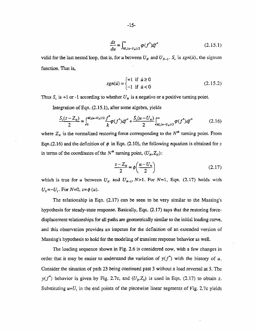
Integration of Eqn. (2.15.1), after some algebra, yields
(2.16)
where ZN is the normalized restoring force corresponding to the Nth turning point. From
Eqn.(2.16) and the definition of l/J in Eqn. (2.10), the following equation is obtained for z
in terms of the coordinates of the Nth turning point, (UN' ZN) :
(2.17)
which is true for u between UN and UN-1' N> 1. For N =1, Eqn. (2.17) holds with
UO=-U1 • For N=O, z=l/J (u).
The relationship in Eqn. (2.17) can be seen to be very similar to the Massing's
hypothesis for steady-state response. Basically, Eqn. (2.17) says that the restoring force
displacement relationships for all paths are geometrically similar to the initial loading curve,
and this observation provides an impetus for the definition of an extended version of
Massing's hypothesis to hold for the modeling of transient response behavior as well.
The loading sequence shown in Fig. 2.6 is considered now, with a few changes in
order that it may be easier to understand the variation of y(f*) with the history of u.
Consider the situation of path 23 being continued past 3 without a load reversal at 3. The
y(f*) behavior is given by Fig. 2.7c, and (U2,Z2) is used in Eqn. (2.17) to obtain z.
Substituting u=U1 in the end points of the piecewise linear segments of Fig. 2.7c yields
-16-
Fig. 2.7a for u=U1• Thus the extension of path 23 passes through 1. For any further
loading in the positive u direction, y(f*) behavior is as in Fig. 2.7a. For purposes of
determination of z from this instant on, it as if the loop 1231 never happened at all.
Consider a different situation wherein path 56 is continued in decreasing u direction
past U6 • The y(f*) behavior is given by Fig. 2.7f, and (Us' Zs) is used in Eqn. (2.17) to
obtain z until the path reaches 4, after which Fig. 2.7d controls the behavior of y(f*); for
purposes of determination of z from this instant on, the fact that the loop 4564 occurred is
of absolutely no consequence. If u continues to decrease past U4 , Fig. 2.7d controls y(f*),
and (U3,Z3) is used in Eqn. (2.17) until the path reaches 2, when Fig. 2.7b comes into
effect. On the other hand, if there is a load reversal at some point between U2 and U4 , the
y(f*) is governed by Fig. 2.7e, and the values of u and z corresponding to that load
reversal are used in Eqn. (2.17) in the determination of z until the path reaches 3, and so
on.
It must be mentioned here that the result of Eqn. (2.17) was derived for the case
where the largest excursion is to the positive u direction (that is, U1>0). In exactly the same
manner, the result can be shown to be true also for the case where the largest excursion is
to the negative u direction (U1<0).
2.3.3 The Extended Massing's hypothesis:
From the similarity between the relations expressed by Eqns. (2.7) and (2.17), it is
possible to extend the Massing's hypothesis originally proposed for steady-state response
to transient dynamic response as well. In his work on the determination of optimal
nonlinear models by applying system identification techniques to inelastic pseudo-dynamic
test data, Jayakumar [24] originally proposed this extension of the Massing's hypothesis
by stipulating the following two rules for the system behavior during complete and
incomplete loops:
-17-
• Rule 1: Incomplete loops
The equation of any hysteretic response curve, irrespective of steady-state or transient
response, can be obtained simply by applying the original Massing rule to the virgin
loading curve using the latest point of loading reversal.
• Rule 2: Completed loops
The ultimate fate of an interior curve under continued loading or unloading can be
determined as follows: Once an interior curve crosses a curve from a previous load cycle,
the load-deformation curve then follows that of the previous cycle.
By showing that these two rules could be used to predict the behavior of the parallel
series Distributed Element model for paths 12 and 23 of Fig. 2.6, he concluded that the two
rules could be used to completely describe the transient hysteretic behavior of the said
model [24]. The following representation for the same rules is felt to be in a form more
amenable to numerical implementation.
Let z=</J (u) be an expression for the initial loading behavior of a system where </J IS
an odd function of u. Let the derivative of the function </J be 'If/, i.e., 'If/(u) == </J'(u), and let
U = {U1'U2'U3' ...... ,UNr be the array of N nested turning points, which is continually
updated in a manner described below. As before, Ui and Zi are the displacement and
normalized restoring force corresponding to the ith load reversal (i=1,2, ... ,N). Thus, UN is
the displacement corresponding to the last load reversal up to the instant under
consideration. Let the next load reversal be at a displacement of Uo' If there are no load
reversals after UN' then the following hypothesis holds with Uo-";ooSv, i.e., +00 or -00
according to whether U>O or u<O. As u moves from UN to Uo, the following rules express
the manner in which (i) the normalized restoring force, z, is determined and (ii) the array U
is updated:
-18-
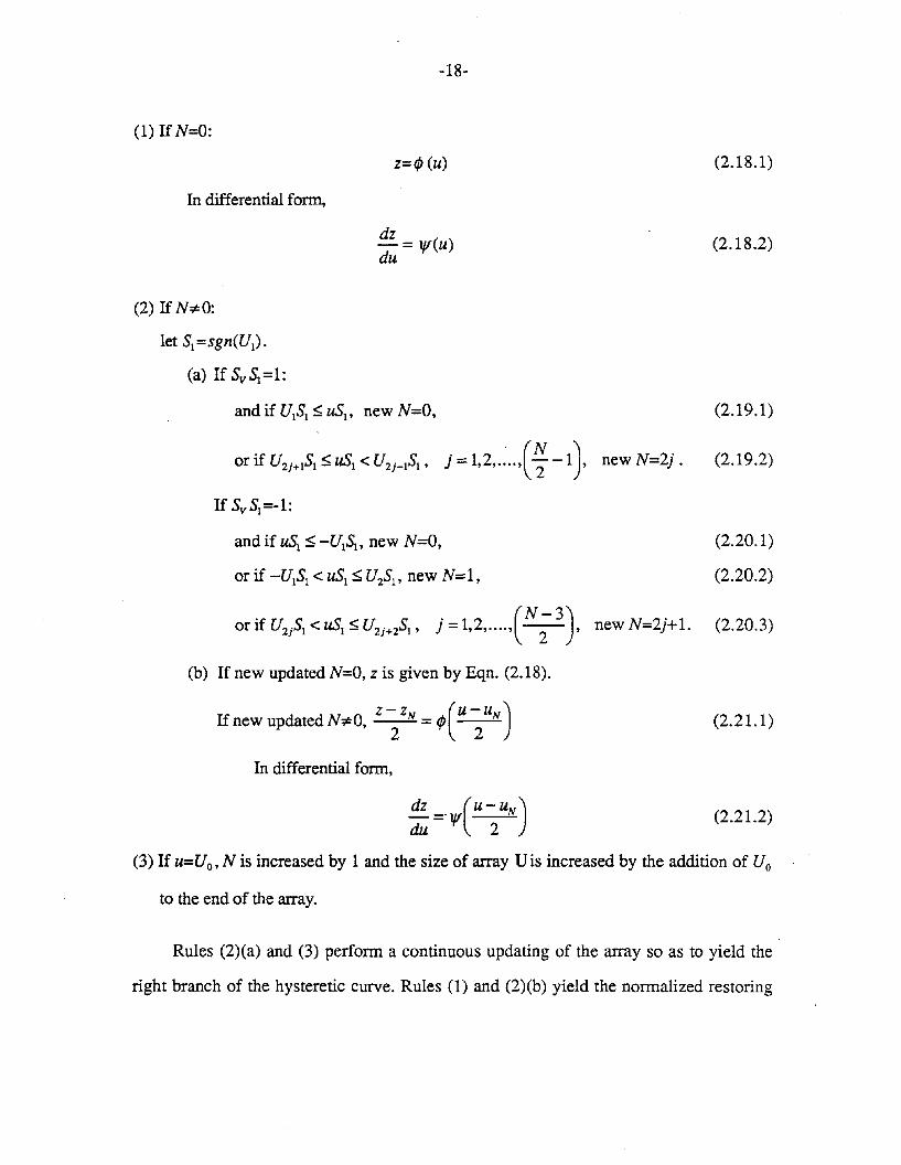
(1) If N=O:
In differential form,
(2) IfN¢O:
let Sl=sgn(U1)·
(a) If SvSl=1:
z=</J (u)
dz- = V'(u)du
(2.18.1)
(2.18.2)
(2.19.1)
(2.19.2)
If SvSl=-l:
and if uS1:::;; -U1S1, new N=O, (2.20.1)
or if -U1S1< uS1:::;; UZSl' new N= 1, (2.20.2)
or if UZjS1 < uS1 :::;; UZj+zSl' j = 1,2,....,(N; 3). new N=2j+1. (2.20.3)
(b) If new updated N=O, z is given by Eqn. (2.18).
z-z (u-U )Ifnew updated N¢O, T = </J 2 N
In differential form,
(2.21.1)
(2.21.2)dz =-V'(U- UN)du 2
(3) If u=Uo, N is increased by 1 and the size of array U is increased by the addition of Uo
to the end of the array.
Rules (2)(a) and (3) perform a continuous updating of the array so as to yield the
right branch of the hysteretic curve. Rules (1) and (2)(b) yield the normalized restoring
-19-
force z corresponding to the displacement u. Even though all the branches of the restoring
force diagram obey the same relationship given by Eqn. (2.21) (for N*O), since the array
is being updated continually depending on the history of u, the values of UN and ZN that
are used in the equation are different, thus yielding the appropriate hysteretic branch.
One point of interest here is in the nondependence of the differential formulation on
the quantity ZN as evidenced in Eqn. (2.18.2) and Eqn. (2.21.2). Use of the differential
formulation does not involve memorizing the array of the values of z corresponding to the
nested turning points. However, an integration needs to be done to obtainz. In dynamical
systems, the equations of motion frequently involve writing expressions for the derivatives
of the state variables. The differential formulation of the Extended Massing's hypothesis is
very convenient for the purpose.
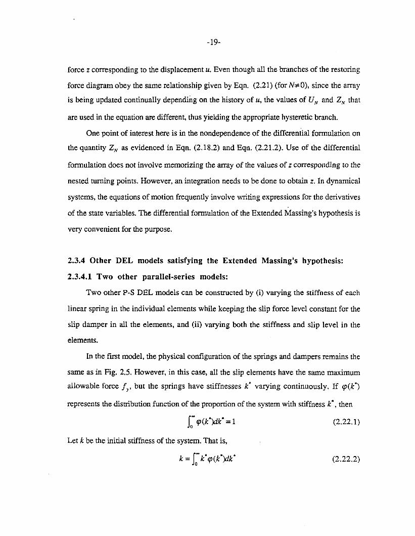
2.3.4 Other DEL models satisfying the Extended Massing's hypothesis:
2.3.4.1 Two other parallel-series models:
Two other P-S DEL models can be constructed by (i) varying the stiffness of each
linear spring in the individual elements while keeping the slip force level constant for the
slip damper in all the elements, and (ii) varying both the stiffness and slip level in the
elements.
In the fIrst model, the physical confIguration of the springs and dampers remains the
same as in Fig. 2.5. However, in this case, all the slip elements have the same maximum
allowable force I y ' but the springs have stiffnesses k* varying continuously. If q>(k*)
represents the distribution function of the proportion of the system with stiffness k *, then
(2.22.1)
Let k be the initial stiffness of the system. That is,
(2.22.2)
-20-
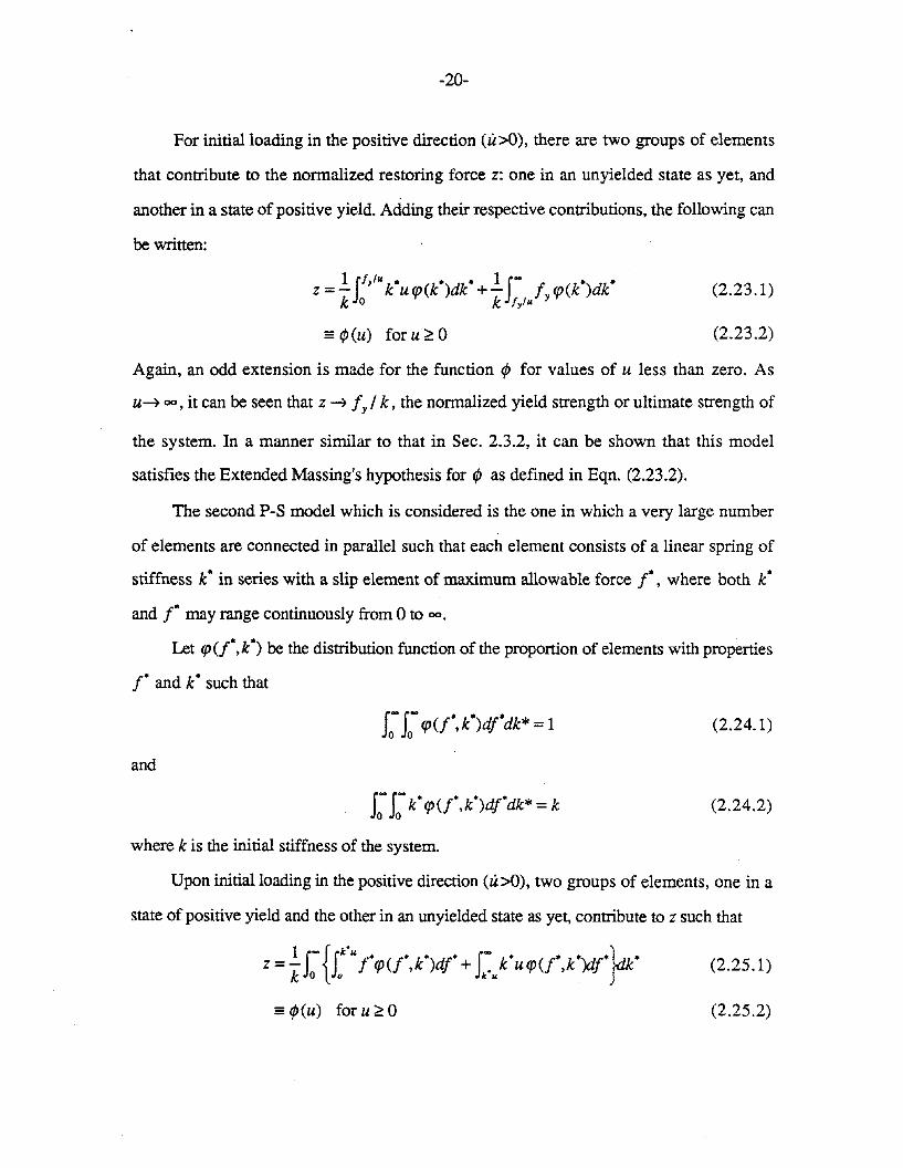
For initial loading in the positive direction (U>O), there are two groups of elements
that contribute to the normalized restoring force z: one in an unyielded state as yet, and
another in a state of positive yield. Adding their respective contributions, the following can
be written:
== ifJ(u) for u ~ 0
(2.23.1)
(2.23.2)
Again, an odd extension is made for the function ifJ for values of u less than zero. As
u~ 00, it can be seen that z~ f y I k, the normalized yield strength or ultimate strength of
the system. In a manner similar to that in Sec. 2.3.2, it can be shown that this model
satisfies the Extended Massing's hypothesis for ifJ as defined in Eqn. (2.23.2).
The second P-S model which is considered is the one in which a very large number
of elements are connected in parallel such that each element consists of a linear spring of
stiffness k* in series with a slip element of maximum allowable force f*, where both k*
and f* may range continuously from 0 to 00.
Let <p (f*, k *) be the distribution function of the proportion of elements with properties
f* and k * such that
and
S: S: k* <p(f*,k*)df*dk* = k
(2.24.1)
(2.24.2)
where k is the initial stiffness of the system.
Upon initial loading in the positive direction (U>O), two groups of elements, one in a
state of positive yield and the other in an unyielded state as yet, contribute to z such that
== ifJ(u) for u ~ 0
(2.25.1)
(2.25.2)
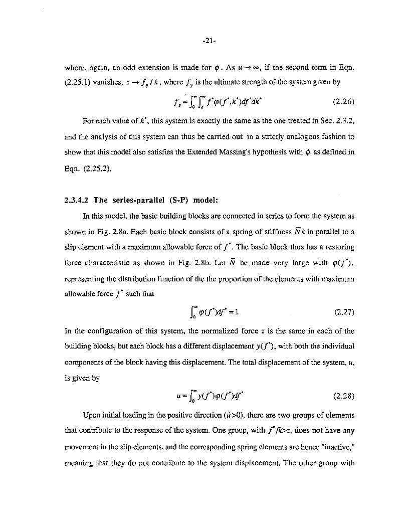
-21-
where, again, an odd extension is made for </>. As u~ 00, if the second term in Eqn.
(2.25.1) vanishes, z~ f y / k, where f y is the ultimate strength of the system given by
(2.26)
For each value of k*, this system is exactly the same as the one treated in Sec. 2.3.2,
and the analysis of this system can thus be carried out in a strictly analogous fashion to
show that this model also satisfies the Extended Massing's hypothesis with </> as defined in
Eqn. (2.25.2).
2.3.4.2 The series-parallel (S-P) model:
In this model, the basic building blocks are connected in series to form the system as
shown in Fig. 2.8a. Each basic block consists of a spring of stiffness Nk in parallel to a
slip element with a maximum allowable force of f*. The basic block thus has a restoring
force characteristic as shown in Fig. 2.8b. Let N be made very large with qJ(f*) ,
representing the distribution function of the the proportion of the elements with maximum
allowable force f* such that
(2.27)
In the configuration of this system, the normalized force z is the same in each of the
building blocks, but each block has a different displacement y(f*), with both the individual
components of the block having this displacement. The total displacement of the system, u,
is given by
(2.28)
Upon initial loading in the positive direction (U>O), there are two groups of elements
that contribute to the response of the system. One group, with f* /k>z, does not have any
movement in the slip elements, and the corresponding spring elements are hence "inactive,"
meaning that they do not contribute to the system displacement. The other group with
-22-
f* /k<z has slipping elements and "active" springs, meaning that the springs have relative
displacements and contribute to the system displacement Hence,
u = 1,"(z - nq>(f')dt'
== ~(z) for z ~ 0
(2.29.1)
(2.29.2)
Let an odd extension of ~ be made for z<O. The initial loading curve here expresses u as a
function of z. Let the inverse function of ~ be t/J • That is, the initial loading curve may also
be expressed as:
z=t/J (u) (2.29.3)
The restoring force characteristic of the S-P model has two significant differences
from the P-S modeL By differentiating Eqn. (2.29.1), it may be shown that dz/du ~ 00 as
u ~O, and ~k as u ~ 00. That is, this system has an infinite initial stiffness and an
asymptotic stiffness k at large deformations. It does not have an ultimate force level as did
the P-S model in Sec. 2.3.2.
By observing the y(f*) behavior of a few nested loops as was done for the case of
the P-S model in Fig. 2.7, it can be shown that the active elements of the system
contributing to the system compliance (where the compliance is the inverse of the stiffness)
satisfy the following inequality:
(2.30.1)
Since the springs in the active elements are connected in series, the compliances of the
elements add to give the total system compliance, du/dz. Hence,
du is-''(Z-ZN)12 * *-= qJ(f)dfdz 0
(2.30.2)
is true for the last nested loop. Integration of Eqn. (2.30.2), after some algebra, and
making use of the odd property of ~ yields
-23-
U-2UN=~(Z-2ZN)
Using the inverse function of ~, namely, ¢ , the following may be written
z -2ZN =¢(U-2UN)
(2.31)
(2.32)
which is true for the last nested loop.
It is thus seen that the S-P system also satisfies the relations of the Extended
Massing's hypothesis.
2.3.4.3 Stiffness- and strength-degrading model:
The physical configuration of this model is of the P-S type considered in Sec. 2.3.2.
The only difference is in the behavior of the slip element in each building block. In the
model considered here, the slip element "breaks," once it has slipped a certain specified
displacement. For subsequent loading, the system cannot recover the stiffness and strength
of this building block. This results in a stiffness- and strength- degrading model. Cifuentes
[13] used such a model for the identification of reinforced concrete structures. A typical
restoring force diagram of this model for a structure has been reproduced from his work
[13] in Fig. 2.9. The deterioration in both system stiffness and strength as the deformation
increases is evident from the figure.
Assume that the elastoplastic unit of stiffness k and ultimate strength j* breaks when
the relative displacement of the slip element reaches an absolute value equal to Il times the
yield displacement f* /k, Il (>0) being the same for all the elastoplastic units. The behavior
of such an elastoplastic unit may be used for the modeling of the failure of concrete because
of spalling in the compressive loading direction and because of cracking in the tensile
loading direction.
(2.33)
-24-
Let a be the largest absolute value of the displacement until the instant under
consideration. Then those elements that have broken thus far satisfy the inequality
f* ~.3!!:A+1
To account for the removal of the broken elements, the updated ijJ(f*) is defined as
follows:
10 for O~f*~~
ijJ(f*) = A + 1* * ka
qJ(f) for f > A +1
(2.34)
(2.35.1)
where qJ(f*) is the distribution function of the proportion of the system with strength f*
(O~f*<00) in the virgin state of the system.
Let ~(u) be dermed as
¢(u) == 1. rkuf*ijJ(f*)df* + uS" ijJ(f*)df* for u>°
kJo ku
¢(u)=-¢(-u) foru<O (2.35.2)
For all nested loops of u within [-a,a], the system essentially behaves as the P-S
model discussed in Sec. 2.3.2 with a distribution function ijJ(f*) as in Eqn. (2.34). Thus,
this model satisfies the Extended Massing's hypothesis, and z may be obtained from
(2.36)
for N*O. If N=O, z is given by ¢(u).
There is one qualifying remark that must be made here about the function t/J. The
function t/J in Eqn. (2.17) does not vary with the history of u. The corresponding function
¢ for this model used in Eqn. (2.36) changes, depending on the history of u (actually, on
a, the largest absolute value of the displacement). There is thus an implicit memory-
dependence which is described by Eqns. (2.34) and (2.35).
-25-
Once u passes ± a, the parameter a assumes the value of the new maximum of lui, ijJ
changes as per Eqn. (2.34), ¢ changes as per Eqn. (2.35) and the normalized restoring
force z is given by Eqn. (2.36).
A remark that may be made here regards a difference in the two memory parameters
U and a. U is an array of nested turning points that can be completely "forgotten" (that is,
disregarded) once the system displacement passes either ±U1 • The fact that the nested loops
occurred has no future significance in the determination of z. In contrast, a represents an
effect that cannot be recovered since once the elements are broken, they cannot contribute to
the system response behavior any more. a is a cumulative damage parameter, and cannot be
"forgotten." This property of a ensures that the system has a permanent degradation of
system properties.
2.3.5 Curvilinear models with one or two hidden state variables:
2.3.5.1 The endochronic models:
Endochronic theories of material behavior were introduced and employed by Valanis
[50] to develop a constitutive law for metals which characterizes strain-hardening,
unloading behavior, cross-hardening (for example, the effect of pretwist on axial
behavior), the alteration of hysteresis loops with continued cyclic straining and sensitivity
to strain rate. Bazant and Bhat further developed the theory to describe the liquefaction of
sand, and the failure of concrete [7].
Fundamentally, the endochronic models do not make use of a yield condition as do
most classical theories of plasticity, but instead use a quantity referred to as the intrinsic
time. This quantity is introduced into the constitutive laws of viscoelasticity in place of the
real time. By starting with a one-dimensional Maxwell model, Bazant and Bhat [7]
constructed the following version of a simple endochronic model:
-26-
1. da = Ede - - aldelZ
(2.37.1)
where a is the stress, e is the strain, E is the Young's modulus and Z is the relaxation
time of the material. Equivalently,
. E· 1 '·1a= e--aeZ
(2.37.2)
where, as usual,the dot superscript refers to the derivative with respect to time.
The model in Eqn. (2.37) is rate-independent, and the stress approaches the limit ZE
asymptotically for large strains. It can be seen that Eqn. (2.37) is a complete description of
the material behavior. There are no yield conditions, hardening rules, etc. However, having
a representation as simple as this does have its price. The behavior of such models can be
quite nonphysical. More will be said about this in Chapter 4.
2.3.5.2 The Wen-BODe model and the Casciyati models:
A differential equation model for hysteresis originally proposed by Bouc was later
generalized by Wen [53,54]. The model is widely used in structural dynamics, especially in
the stochastic response analysis of hysteretic systems. Essentially, the model requires that
the normalized hysteretic restoring force satisfy the frrst-order, nonlinear differential
equation
(2.38)
where the parameters A, f3, r, 1], v and n govern the amplitude, shape of the hysteresis
loop and the smoothness of transition into the inelastic range. The total restoring force of
the system, f, is again given by Eqn. (2.1). The ability of this model to depict curvilinear
hysteretic behavior has been shown for the case n=l in [54]. In the same paper, Wen
extended the above model to include stiffness- and/or strength-degradation of the restoring
-27-
force. A hysteretic energy dissipation, which is a measure of the cumulative effect of the
severe response and repeated oscillations, is defined as follows:
E(~) = (1- a)kS;Z( -r)u( -r)d-r (2.39)
where k and a are, as usual, the initial stiffness and the post-yielding stiffness ratio of the
system. Stiffness- and strength-degradation can be jointly introduced by prescribing A as a
degrading function of E(t). That is,
A(t) = Ao - 0AE(t) (2.40.1)
(2.40.2)
where 0A is the deterioration rate and Ao is the value of A at the commencement of loading.
Similarly, strength-degradation can be introduced by
v(t) = vo+ovE(t)
and stiffness-degradation by
11(t) = 11o+o1/E(t) (2.40.3)
where Ov and 01/ control the degradation rates, and Vo and 110 are the initial values of v
and 11, respectively, at the commencement ofloading.
In the case n=l, 11= v=l, A=E, f3 =1/2, r =0, it can be seen that the z-u relationship
as per Eqn. (2.38) is exactly the same as the (J -e relationship expressed by Eqn. (2.37.2)
for the simple endochronic model. The similarity in the initial loading behavior of these
models was noted first by Jayakumar [24]. Thus, even though the endochronic model and
the Wen-Bouc model were motivated by different reasons and for application to different
fields of research, their behavior is very similar. For this reason, it is felt that it will not be
inappropriate to refer to the group of models included in this section as the endochronic
group of models.
The family of endochronic models exhibit certain unrealistic characteristics that are
quite inconsistent with observed physical behavior. These will be enumerated in detail in
Chapter 4. In an effort to minimize one such unrealistic feature of the Wen-Boue model,
-28-
namely, the possible nonclosure of hysteresis loops, Casciyati [10] proposed the following
amendment for the case n=1:
i = Au':" f3lulz+ rulzl+ <5lulsgn(z) (2.41)
where <5 is a parameter intended to control loop closure.
As a final remark, it may be mentioned that the endochronic models can be easily cast
in the DEQ category described in Sec. 2.1. For nondegrading systems, this is achieved by
the addition of the hidden state variable, z, to the conventional state variables u and u to
describe the system response. For degrading models, the inclusion of z as well as E(t) can
be done to formulate the system in a purely history-independent fashion involving an
expanded number of state variables.
2.4 The DEQ category of hysteretic models:
Random vibration studies of linear systems have been used very successfully to
determine various statistical measures of the response of single- and multi-degree-of
freedom systems subjected to random excitation. Unfortunately, to date there are no
systematic analytical methods to obtain closed-form solutions to the stochastic response of
a general nonlinear dynamical system. The scarcity of exact solutions has necessitated the
analytical development of approximate solution techniques.
One of the most promising of such approximate analysis techniques is the method of
equivalent linearization. In the case of random excitation, this method approximates the
original set of nonlinear stochastic differential equations with a more tractable linear set
which are easily analyzed. The general results oflwan [22], Atalik and Utku [4], Caughey
[12], Spanos and Iwan [45] provide a sound foundation for this method. As of now, this
method is capable of satisfactorily handling nonlinear systems that can be described by a set
of finite number of single-valued, possibly nonlinear, ordinary differential equations. The
keyword is "single-valued," meaning that the equations cannot be history-dependent.
-29-
Caughey [11] used the additional Krylov-Bogoliubov (K-B) approximation to examine the
random response of a bilinear hysteretic system subjected to white noise excitation.
However, it has been shown that this method does not produce wholly satisfactory results
when the response is wide band (as in the case of elastoplastic or nearly elastoplastic
systems).
If, in some manner, the history dependence of the system could be "removed" by the
addition of one or more state variables, rendering the expanded system description history
independent, then the theory of equivalent linearization could be used in the analysis of
hysteretic systems as well. It is precisely with this point in mind that several of the models
described in this chapter have been proposed. The hysteretic behavior of these systems is
controlled by the behavior of the instantaneous values of the newly included state variables,
which are "internal" or "hidden" in the system. This is not to say that all physical hysteretic
systems can be formulated in such a representation; the Distributed Element models with a
continuous hysteretic characteristic have not yet been shown to have such a representation.
But for systems that do, for example, the piecewise-linear hysteretic models, the
endochronic models, etc., the method has been used to calculate the stochastic response of
the systems when subjected to random excitations [3,48,53]. Being able to perform the
approximate analysis of hysteretic systems in this fashion has been the driving force behind
the quest of the DEQ representation for the systems.
2.5 A history-independent representation for a Distributed Element model:
It may be mentioned here that it is possible to derive a history-independent
representation even for the Distributed Element models; for instance, the equations of
motion of a single-degree-of-freedom system whose restoring force behavior is described
by the parallel-series model (Sec. 2.3.2) can be written as
-30-
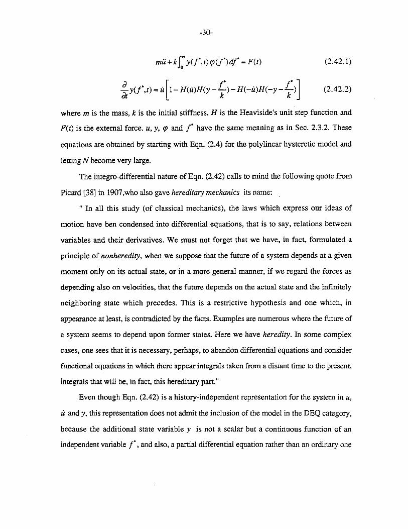
mu+kf: y(f*,t)qJ(f*)df* = F(t)
~y(f',t)= u [1- H(u)H(y - ~. ) - H(-u)H(-y - ~.)]
(2.42.1)
(2.42.2)
where m is the mass, k is the initial stiffness, H is the Heaviside's unit step function and
F(t) is the external force. u, y, qJ and f* have the same meaning as in Sec. 2.3.2. These
equations are obtained by starting with Eqn. (2.4) for the polylinear hysteretic model and
letting N become very large.
The integro-differential nature of Eqn. (2.42) calls to mind the following quote from
Picard [38] in 1907,who also gave hereditary mechanics its name:
" In all this study (of classical mechanics), the laws which express our ideas of
motion have ben condensed into differential equations, that is to say, relations between
variables and their derivatives. We must not forget that we have, in fact, formulated a
principle of nonheredity, when we suppose that the future of a system depends at a given
moment only on its actual state, or in a more general manner, if we regard the forces as
depending also on velocities, that the future depends on the actual state and the infmitely
neighboring state which precedes. This is a restrictive hypothesis and one which, in
appearance at least, is contradicted by the facts. Examples are numerous where the future of
a system seems to depend upon former states. Here we have heredity. In some complex
cases, one sees that it is necessary, perhaps, to abandon differential equations and consider
functional equations in which there appear integrals taken from a distant time to the present,
integrals that will be, in fact, this hereditary part."
Even though Eqn. (2.42) is a history-independent representation for the system in u,
u and y, this representation does not admit the inclusion of the model in the DEQ category,
because the additional state variable y is not a scalar but a continuous function of an
independent variable f* , and also, a partial differential equation rather than an ordinary one

-31-
is involved. Currently, there are no techniques that can help perfonn a direct linearization of
this system of equations. An extension of the theory of equivalent linearization to include
representations such as this would prove very beneficial in the analysis of curvilinear
hysteretic systems.
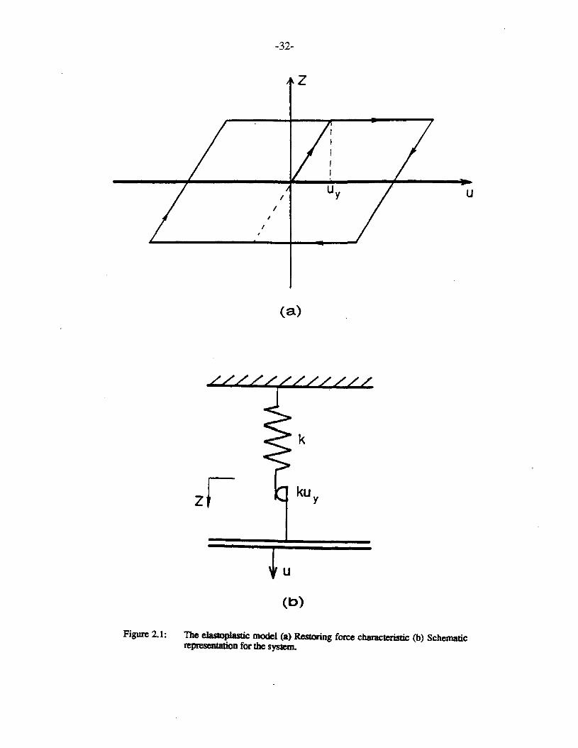
I
,
-32-
z
I
I
(a)
u
(b)
Figure 2.1: The elastoplastic model (8) Restoring force characteristic (b) Schematicrepresentation for the system.
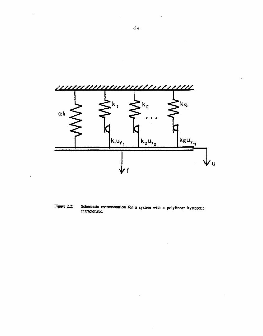
-33-
k2 uY2
Figure 2.2: Schematic representation for a system with a polylinear hystereticcharacteristic.
u
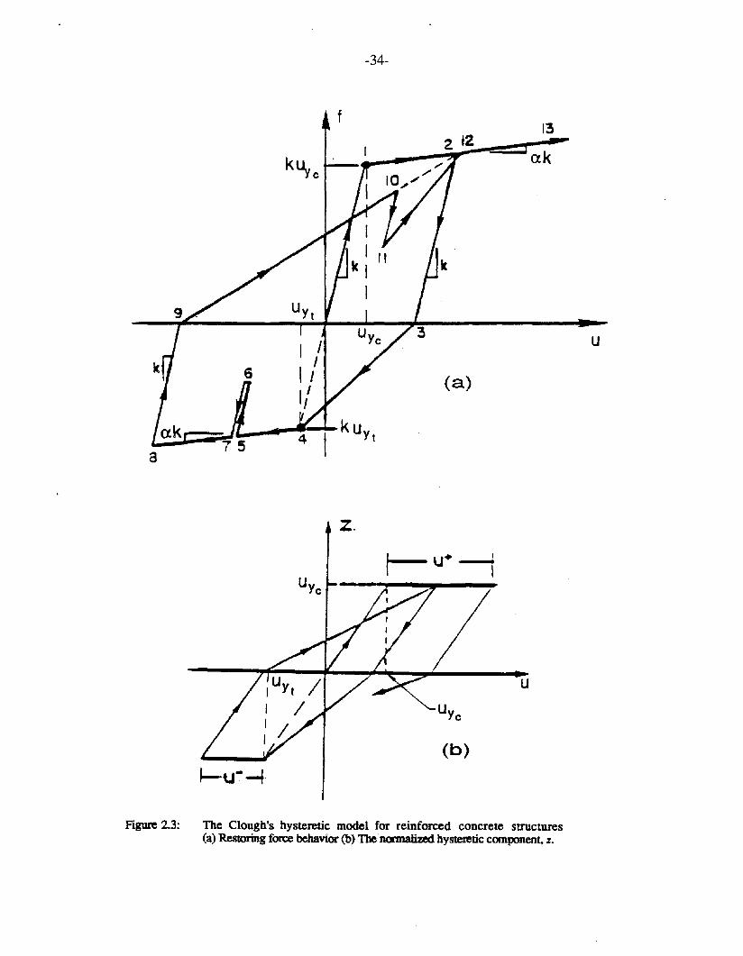
-34-
f13
L_.~-"'~~12rl~2~-::::!,-;;-k akUyc
(a)
z.
u
(b)
Figure 2.3: The Clough's hysteretic model for reinforced concrete structures(a) Restoring force behavior (b) Thenmnalized hysteretic component. z.
u
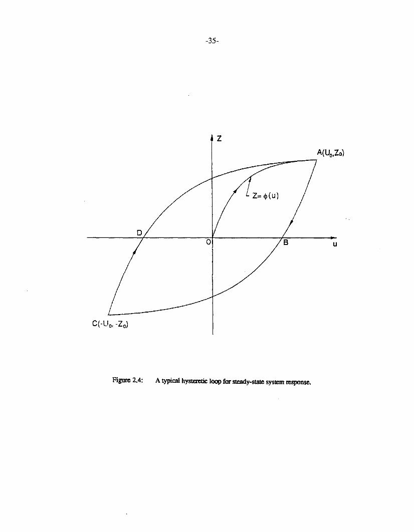
-35-
z
Figure 2.4: A typical hysteretic loop for steady-state system response.
u
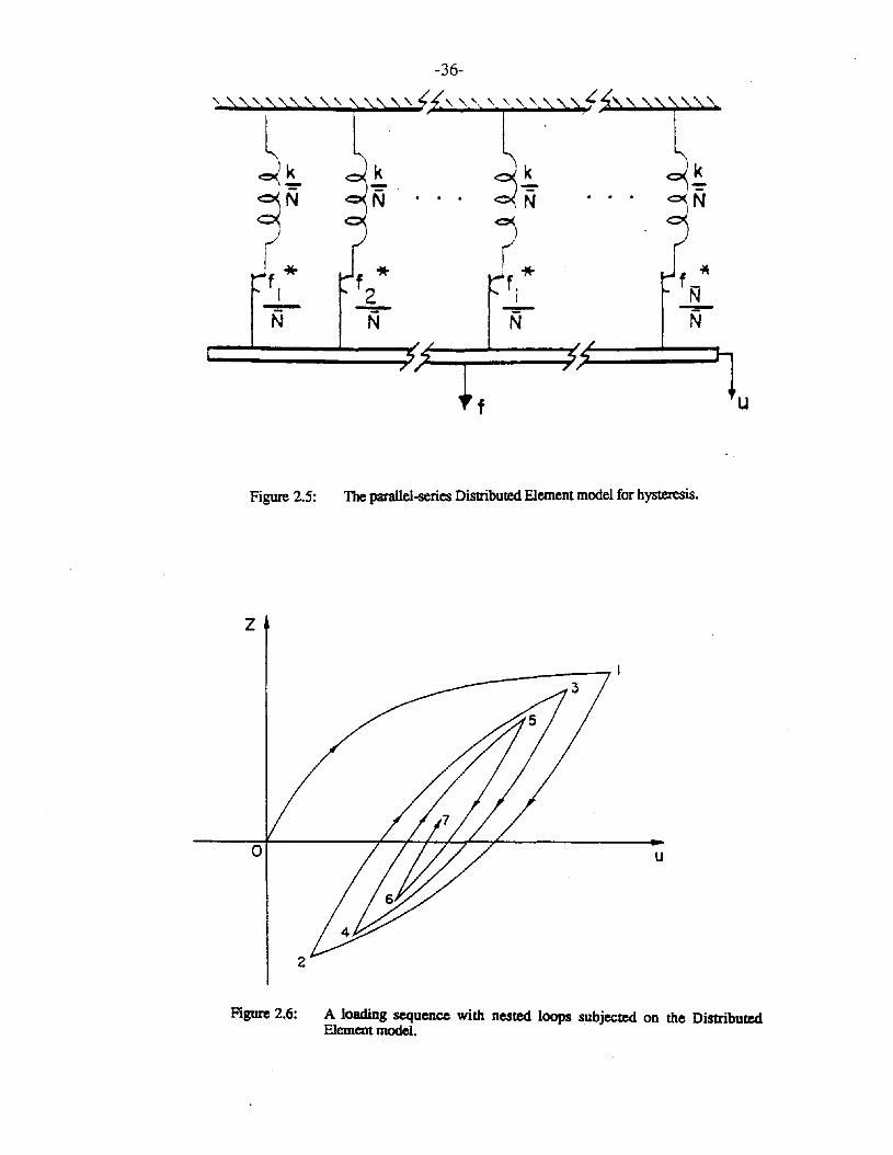
-36-
"- , £' '\"" \\\\4'
l ' l)~~ k
~*~N N . . . . . .~ ~I
f* f * f _-YtI 2 NN -=- - NN N
f u
Figure 2.5: The parallel-series Distributed Element model for hysteresis.
z
o
2
u
Figure 2.6: A loading sequence with nested loops subjected on the DistributedElement model.
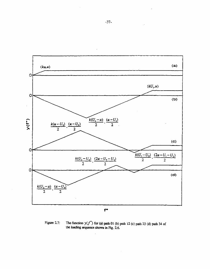
-37-
(ku.u) (a)
o~=------------------------_,
(c)
k(UI-u) (u-V1)
2 2
ok-----------------:;:::7~-----_,(b)
O~=---------------...::::::.."""=::::""~...::::------_t
•~-'"
(d)
k(U1 - U2) (2u - U1 - V2)
2 . 2k(U3 -U2 ) (2U-U2 -U3)
2 2
k(V3 -u) (u-U3)
2 ' 2
O~---------~:::::::....---::::~:_::::::::"'...:::::::...----___i
Figure 2.7: The function y(f*) for (a) path 01 (b) path 12 (c) path 23 (d) path 34 ofthe loading sequence shown in Fig. 2.6.
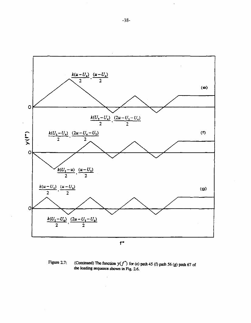
-38-
l(u - U,,) (u - U,,)2 · 2
(e)
o1L.------~~__:7'L-----:::~_r~----1
(f)
l(U, - U~) (2u - U, - U~)
2 · 2
l(U5 - u) (u - Us)
2 • 2
l(U5 - U~) (2u - U~ - Us)2 2
t~-~oL-------'?L.--~~__:7'L-----:::~_r~----1
l(U5 - Ut» (2u-U5 - Ut»
2 ' 2
f*
Figure 2.7: (Continued) The function y(f·) for (e) path 45 (f) path 56 (g) path 67 ofthe loading sequence shown in Fig. 2.6.
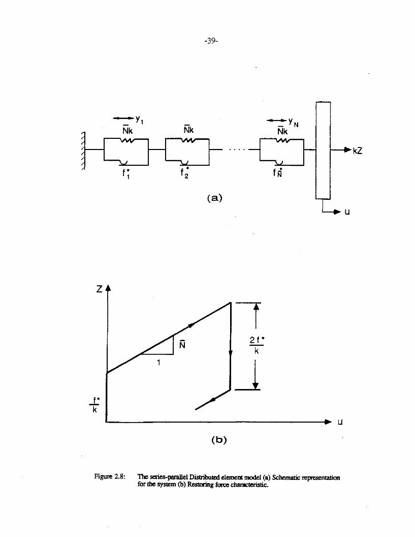
-39-
f*,
-y_ NNk
"-"'kZ
(a)
u
Figure 2.8: The series-parallel Distributed element model (a) Schematic representationfor the system (b) Restoring force charac1eristic.
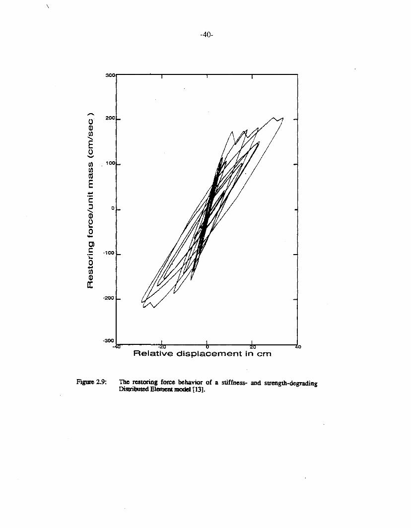
\
-40-
3oo.....----..,...------r-------,~---__,
-0 200
(I)fIJ......E0-fIJ 100
fIJtTJ
E~
C::J 0......(1)
e0....C)C -100'i:0+'"fIJ(I)
a:-200
-300"-----'"*"'----4------.:b.----~0Relative displacement in cm
Figure 2.9: The restoring force behavior of a stiffness- and strength-degradingDistributed Element model [13].
-41-
CHAPTER 3
AN IDENTIFICATION METHOD FOR HYSTERETIC SYSTEMS
3.1 Introduction
The identification of dynamic models through the use of experimental data is a
problem of considerable importance in earthquake engineering. The major goal of the
identification process is to characterize or to "identify" accurately the response behavior of a
structure subjected to strong ground shaking. Considerable effort has been devoted to
determining algorithms and techniques for estimating optimal models from data.
Generally speaking, most of the identification techniques in the past have been
parametric; that is, they seek to detennine the value of the parameters in an assumed model
of the system to be identified. By contrast, nonparametric methods, for example, those by
Masri and Caughey [31], Volterra [52], et al., seek the best functional representation of the
system without any a priori assumptions about the model.
The identification method outlined in this chapter determines a model representation
for nonlinear systems in which the slopes of the loading and unloading paths depend only
on the instantaneous value of the restoring force. The endochronic models described in
Chapter 2 with one additional state variable, for example, the Wen-Bouc hysteretic model,
have such a representation. So does the bilinear system. The method involves a search in
function space to determine an optimal representation of the system. For this reason, the
method can be thought of as a nonparametric identification technique.
The following section describes the technique used for identifying the nonlinear
behavior of a system. Examples of the identification of three different hysteretic systems
are then enumerated. In each case, the adequacy of the optimal model to describe the
original system is examined by comparing their respective responses to a second excitation.
-42-
Some of the significant advantages of the identification method are listed in the final
section.
3.2 The identification procedure:
Let the equation of motion of a single-degree-of-freedom oscillator be given by the
following equations
mil +cu + aku +(1- a)kz = -ma(t)
i = itH(U)!I(Z) + itH(-U)!2(Z)
(3.1)
(3.2)
where u is the relative displacement of the oscillator subjected to the base excitation aCt), z
is the normalized hysteretic restoring force, m is the mass, k is the initial stiffness, a k is
the post-yielding stiffness, c is the viscous damping coefficient, H is the Heaviside's unit
step function, and 11 and 12 are single-valued functions of z. For a given value of z, it may
be noted that k/1(z) and kI2 (z) are the instantaneous system stiffnesses when U>O and
U<O, respectively.
The endochronic models with one additional state variable described in Chapter 2 can
be represented in the above fashion. For instance, for the Wen-Bouc hysteretic model
(Eqn. 2.38), the functions 11 and 12 are given by
11(z) = 2.. [A - vlzl"-l(J3 z- rlzl)] (3.3.1)1'/
12(z) = 2.. [A + vlzl"-I(f3z+ rlz/)] (3.3.2)1'/
where A, f3, r, v, 1'/ and nhave the same meaning as in Eqn. (2.38).
Similarly, for the bilinear model (Eqn. 2.2), the functions 11 and 12 are given by
11(z) = 1-H(z - u) (3.4.1)
12(z)=1-H(-z-uy ) (3.4.2)
-43-
Assume that the ineasurements for aCt) and il are available over a certain time interval
[O,T]. The corresponding displacement, U, and the velocity, li, can be found either by
direct measurement or by integration of il. Assume also that the values of m, e, k and a
have already been obtained by other measurements. For instance, the values of k and a
may be determined by performing a monotonic loading test. Eqn. (3.1) can be rearranged
to write
ma(t) +mil +eli + akuZ = ---'--------
(1- a)k(3.5)
which yields i on differentiation. Eqn. (3.2) can be used to obtain 11 and 12 , as follows:
12(Z) = ~ H(-li)U
Let the normalized value of z, namely; , be defined as:
where
(3.6.1)
(3.6.2)
(3.7.1)
(3.7.2)
Zmin and Zmax being the minimum and maximum measured values of z. Thus, ; varies from
-1 to +1.
Let the normalized functions g1(;) and g2(~) corresponding to 11(z) and 12(z) be
defined as
(3.8)
where ~ and Z are related as in Eqn. (3.7).
The main idea behind the identification methodology used in this chapter is to estimate
the functions g1 and g2 (and hence 11 and 12) by approximate functions g1 and g2'
respectively, where g1 and g2 are expressed in terms of a set of orthogonal polynomials.
-44-
Without loss of generality, the set of Legendre polynomials, P,,(g), will be used for the
remainder of this chapter. Thus,
N
g1(g)=g1(g)= La/~(g);=0
N
gz<g) =gz<g) = Lb)~(g);=0
(3.9.1)
(3.9.2)
The Legendre polynomials, P"(g), which are solutions of the Legendre's differential
equation, are given by Rodrigues' fonnula to be
p (J;) _ 1 d" ( J; 2 1)",,~ - 2"n! dg " ~ - (3.10)
and they satisfy the following orthogonal property with respect to the weighting function of
unity,
if m=n(3.11)
The next step is to estimate the coefficients, a; and b;, using some error-minimization
criteria. Once these coefficients are determined from the measurements, the system is
completely identified for subsequent analysis. Let the error functions be defined as
E;(N) == J1 [g;(g) - g;(g)]2 dg fori = 1,2-1
(3.12)
In order that the optimum choice of the coefficients minimize the errors Et) and
Et) , the following relations must be satisfied:
dE(N) .
_1_=0 forj=0,1,2, ..... ,Ndaj
dE(N)_2_ =0 for j =0,1,2, ..... ,Ndbj
Use of Eqn. (3.12) in Eqn. (3.13) yields
(3.13.1)
(3.13.2)
-45-
(3.14.1)
where
for i = O,1,2, ..... ,N (3.14.2)
hi' =_2_ for i =O,1,2, .....,N2i+1
(3.14.3)
Either because the data are available only at discrete points and/or because the
computation of the coefficients is done on a digital computer, the trapezoidal algorithm may
have to be used to replace the integrals in Eqn. (3.14) by finite sums.
In summary, given an identification excitation aCt) and the corresponding acceleration,
it, of a single-degree-of-freedom system, a model representation of the type described by
Eqns. (3.1) and (3.2) can be identified by the optimal choice of the coefficients a j and bj
given by Eqn. (3.14). For this choice of coefficients, the functions Jl and J2 are the best
approximation in the least-squares sense to the functions 11 and 12' respectively. Using
Eqns. (3.7) and (3.8), it is possible to write
N -A "" z-zliz) =12(z) = .4.Jbj ~(-)
j=O z,.
with z and z,., as in Eqn. (3.7.2).
(3.15.1)
(3.15.2)
It may be mentioned here that the identification data for 11 and 12 need not be
obtained necessarily from the response of the system to a dynamic excitation. It could also
be obtained from the slopes of the restoring force diagram when the system is subjected to
quasi-static loading. Once the data are obtained, the method of identification of the
-46-
nonlinear restoring force behavior of the system using orthogonal polynomials is
unchanged.
3.3 Identification examples
In this section, three examples of the identification of hysteretic systems by the
method described above are illustrated. The three systems considered are the Wen-Bouc,
the Bilinear and the Distributed Element hysteretic systems. In each case, the system
response to two base excitations is determined. The first of these base excitations, ~ (t),
shown in Fig. 3.1 is a sinusoidal function with a linearly increasing amplitude and serves
as the identification excitation. The response of the system to this excitation is used to
obtain the coefficients a j and hj • and hence the functions J1and J2 which define the
optimal model.
The second base excitation, ~(t), shown in Fig. 3.2, is the N-S component of the
1940 EI Centro earthquake, which serves as the verification excitation. The response of the
optimal model to this excitation is compared with that of the original system to the same
excitation. A favorable comparison is an indication that the optimal model is an adequate
mathematical representation for the original system.
3.3.1 Example 1: The Wen-Bouc hysteretic system
A system whose hysteretic behavior is governed by the Wen-Bouc model (Eqn. 2.38)
is considered with the following values of the parameters: the ratio k/m=1O.0, post-yielding
stiffness ratio a =0.10, viscous damping coefficient c=O.O, A=l.O, f3 =30.0, r =-20.0,
n=1.5. For these values of the parameters, the maximum or yield value of z is about 0.074.
When this system is subjected to the identification excitation ~ (t), its response
displacement and velocity are as shown in Fig. 3.3. Substitution of u and u in Eqn. (3.5)
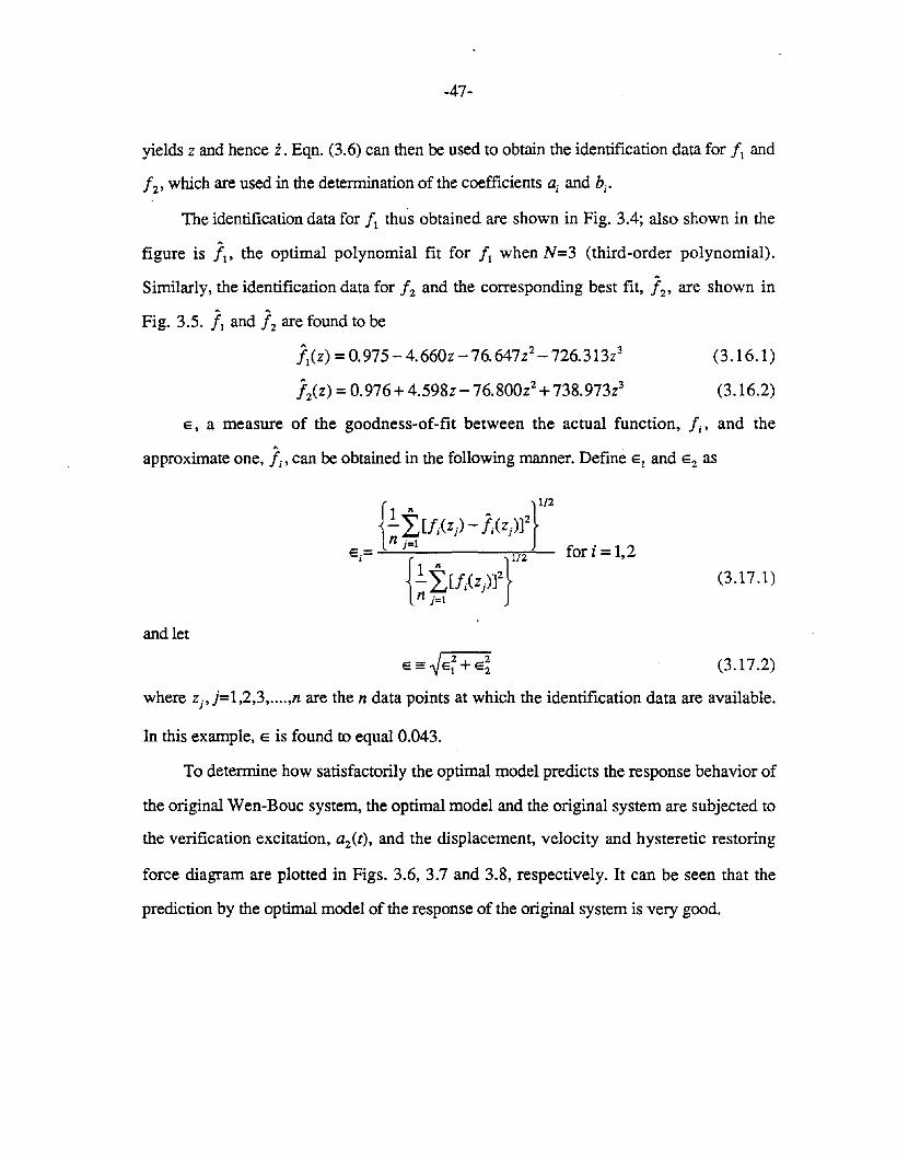
-47-
yields Z and hence i. Eqn. (3.6) can then be used to obtain the identification data for 11 and
12 , which are used in the detennination of the coefficients ai and bi'
The identification data for 11 thus obtained are shown in Fig. 3.4; also shown in the
figure is Jl' the optimal polynomial fit for 11 when N=3 (third-order polynomial).
Similarly, the identification data for 12and the corresponding best fit, J2' are shown inA A
Fig. 3.5. 11 and 12 are found to be
J1(Z) = 0.975 - 4. 660z -76.647z2-726.313z3
J2(Z) = 0.976+ 4.598z -76.800z2+738.973z3
(3.16.1)
(3.16.2)
E, a measure of the goodness-of-fit between the actual function, Ii' and the
approximate one, Jj, can be obtained in the following manner. Define E 1 and E 2 as
(3.17.1)
and let
(3.17.2)
where Zj' j=1,2,3,....,n are the n data points at which the identification data are available.
In this example, E is found to equal 0.043.
To determine how satisfactorily the optimal model predicts the response behavior of
the original Wen-Bollc system, the optimal model and the original system are subjected to
the verification excitation, a2(t), and the displacement, velocity and hysteretic restoring
force diagram are plotted in Figs. 3.6, 3.7 and 3.8, respectively. It can be seen that the
prediction by the optimal model of the response of the original system is very good.
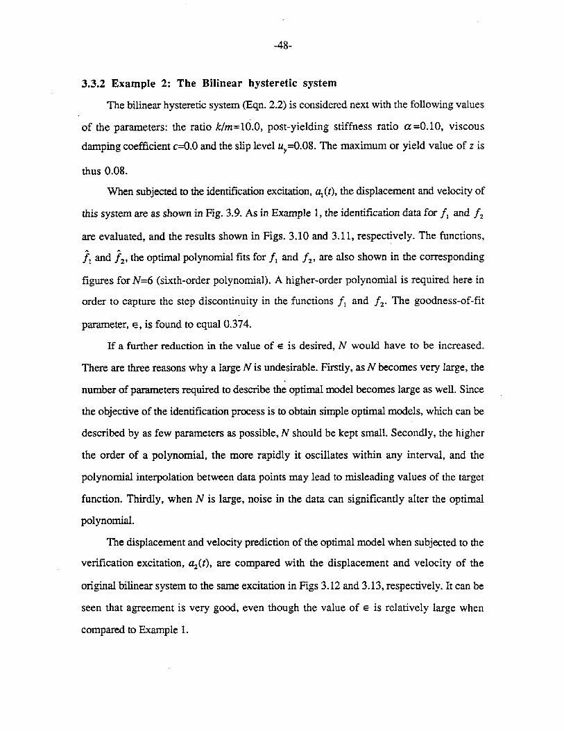
-48-
3.3.2 Example 2: The Bilinear hysteretic system
The bilinear hysteretic system (Eqn. 2.2) is considered next with the following values
of the parameters: the ratio k/m=10.0, post-yielding stiffness ratio a=0.10, viscous
damping coefficient c=O.O and the slip level uy =o.08. The maximum or yield value of z is
thus 0.08.
When subjected to the identification excitation, ~ (t), the displacement and velocity of
this system are as shown in Fig. 3.9. As in Example 1, the identification data for 11 and 12
are evaluated, and the results shown in Figs. 3.10 and 3.11, respectively. The functions,
J1 and J2' the optimal polynomial fits for 11 and 12, are also shown in the corresponding
figures for N=6 (sixth-order polynomial). A higher-order polynomial is required here in
order to capture the step discontinuity in the functions 11 and 12 , The goodness-of-fit
parameter, E, is found to equal 0.374.
If a further reduction in the value of E is desired, N would have to be increased.
There are three reasons why a large N is undesirable. Firstly, as N becomes very large, the
number of parameters required to describe the optimal model becomes large as well. Since
the objective of the identification process is to obtain simple optimal models, which can be
described by as few parameters as possible, N should be kept small. Secondly, the higher
the order of a polynomial, the more rapidly it oscillates within any interval, and the
polynomial interpolation between data points may lead to misleading values of the target
function. Thirdly, when N is large, noise in the data can significantly alter the optimal
polynomial.
The displacement and velocity prediction of the optimal model when subjected to the
verification excitation, a,.(t), are compared with the displacement and velocity of the
original bilinear system to the same excitation in Figs 3.12 and 3.13, respectively. It can be
seen that agreement is very good, even though the value of E is relatively large when
compared to Example 1.
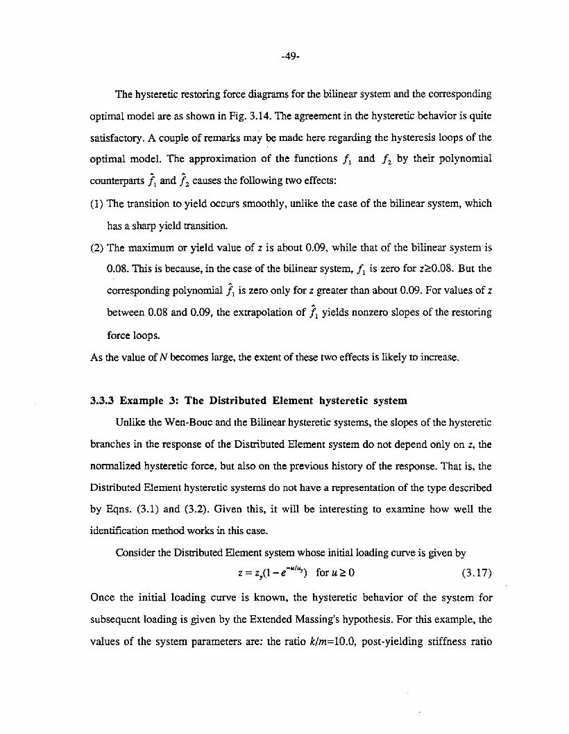
-49-
The hysteretic restoring force diagrams for the bilinear system and the corresponding
optimal model are as shown in Fig. 3.14. The agreement in the hysteretic behavior is quite
satisfactory. A couple of remarks may be made here regarding the hysteresis loops of the
optimal model. The approximation of the functions 11 and 12 by their polynomial
counterparts Jl and J2 causes the following two effects:
(1) The transition to yield occurs smoothly, unlike the case of the bilinear system, which
has a sharp yield transition.
(2) The maximum or yield value of z is about 0.09, while that of the bilinear system is
0.08. This is because, in the case of the bilinear system, 11 is zero for z~0.08. But the
corresponding polynomial Jl is zero only for z greater than about 0.09. For values of z
between 0.08 and 0.09, the extrapolation of J1 yields nonzero slopes of the restoring
force loops.
As the value of N becomes large, the extent of these two effects is likely to increase.
3.3.3 Example 3: The Distributed Element hysteretic system
Unlike the Wen-Bouc and the Bilinear hysteretic systems, the slopes of the hysteretic
branches in the response of the Distributed Element system do not depend only on z, the
normalized hysteretic force, but also on the previous history of the response. That is, the
Distributed Element hysteretic systems do not have a representation of the type described
by Eqns. (3.1) and (3.2). Given this, it will be interesting to examine how well the
identification method works in this case.
Consider the Distributed Element system whose initial loading curve is given by
z = z,(1-e-u'''J) for u ~ 0 (3.17)
Once the initial loading curve is known, the hysteretic behavior of the system for
subsequent loading is given by the Extended Massing's hypothesis. For this example, the
values of the system parameters are: the ratio k/m=1O.0, post-yielding stiffness ratio
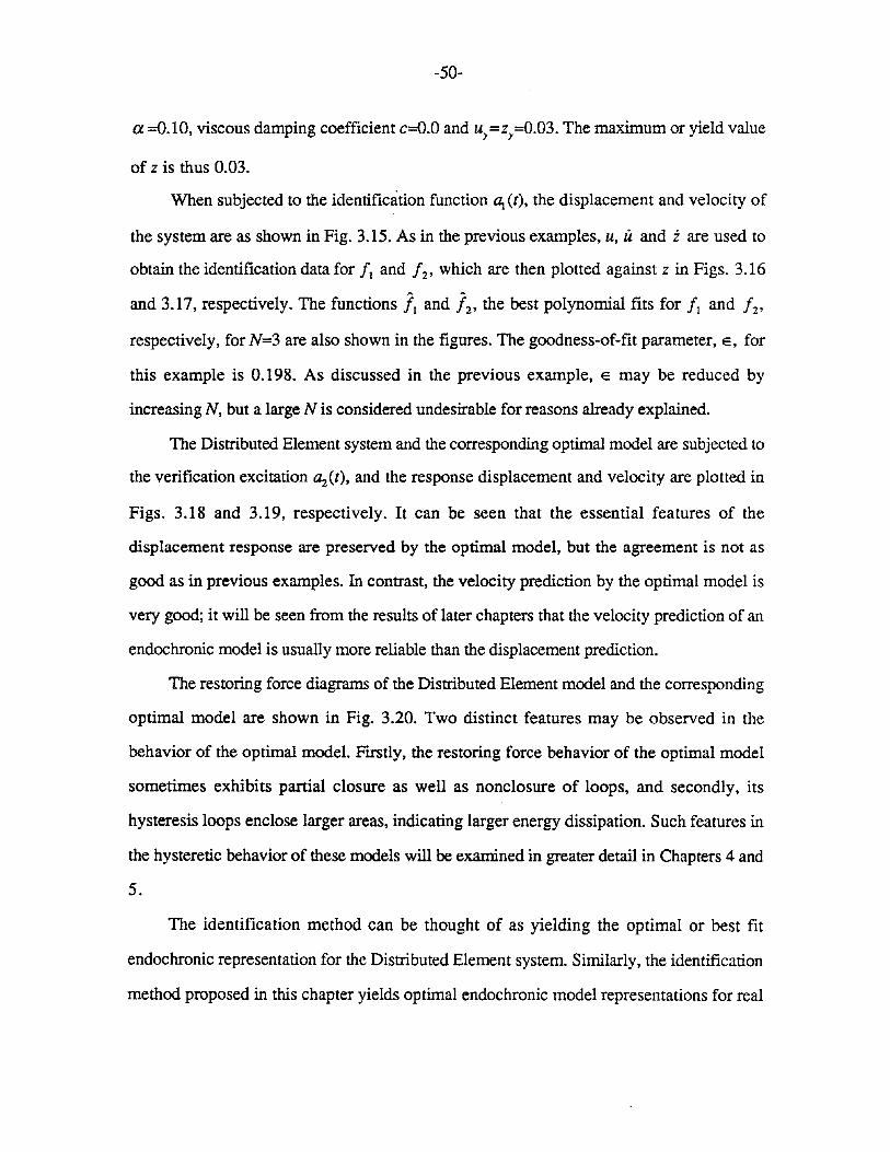
-50-
a =0.10, viscous damping coefficient c=O.O and uy =zy=O.03. The maximum or yield value
of Z is thus 0.03.
When subjected to the identification function ~ (t), the displacement and velocity of
the system are as shown in Fig. 3.15. As in the previous examples, u, U and i are used to
obtain the identification data for /1 and /2' which are then plotted against Z in Figs. 3.16A A
and 3.17, respectively. The functions /1 and /2' the best polynomial fits for /1 and /2'
respectively, for N=3 are also shown in the figures. The goodness-of-fit parameter, E, for
this example is 0.198. As discussed in the previous example, E may be reduced by
increasing N, but a large N is considered undesirable for reasons already explained.
The Distributed Element system and the corresponding optimal model are subjected to
the verification excitation ~(t), and the response displacement and velocity are plotted in
Figs. 3.18 and 3.19, respectively. It can be seen that the essential features of the
displacement response are preserved by the optimal model, but the agreement is not as
good as in previous examples. In contrast, the velocity prediction by the optimal model is
very good; it will be seen from the results of later chapters that the velocity prediction of an
endochronic model is usually more reliable than the displacement prediction.
The restoring force diagrams of the Distributed Element model and the corresponding
optimal model are shown in Fig. 3.20. Two distinct features may be observed in the
behavior of the optimal model. Firstly, the restoring force behavior of the optimal model
sometimes exhibits partial closure as well as nonclosure of loops, and secondly, its
hysteresis loops enclose larger areas, indicating larger energy dissipation. Such features in
the hysteretic behavior of these models will be examined in greater detail in Chapters 4 and
5.
The identification method can be thought of as yielding the optimal or best fit
endochronic representation for the Distributed Element system. Similarly, the identification
method proposed in this chapter yields optimal endochronic model representations for real
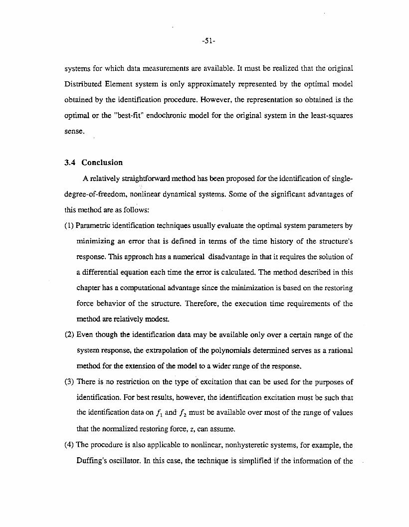
-51-
systems for which data measurements are available. It must be realized that the original
Distributed Element system is only approximately represented by the optimal model
obtained by the identification procedure. However, the representation so obtained is the
optimal or the "best-fit" endochronic model for the original system in the least-squares
sense.
3.4 Conclusion
A relatively straightforward method has been proposed for the identification of single
degree-of-freedom, nonlinear dynamical systems. Some of the significant advantages of
this method are as follows:
(1) Parametric identification techniques usually evaluate the optimal system parameters by
minimizing an error that is defined in terms of the time history of the structure's
response. This approach has a numerical disadvantage in that it requires the solution of
a differential equation each time the error is calculated. The method described in this
chapter has a computational advantage since the minimization is based on the restoring
force behavior of the structure. Therefore, the execution time requirements of the
method are relatively modest.
(2) Even though the identification data may be available only over a certain range of the
system response, the extrapolation of the polynomials determined serves as a rational
method for the extension of the model to a wider range of the response.
(3) There is no restriction on the type of excitation that can be used for the purposes of
identification. For best results, however, the identification excitation must be such that
the identification data on /1 and /2 must be available over most of the range of values
that the normalized restoring force, z, can assume.
(4) The procedure is also applicable to nonlinear, nonhysteretic systems, for example, the
Duffing's oscillator. In this case, the technique is simplified if the information of the
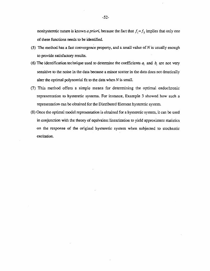
-52-
nonhysteretic nature is known Q priori, because the fact that /1 = /2 implies that only one
of these functions needs to be identified.
(5) The method has a fast convergence property, and a small value of N is usually enough
to provide satisfactory results.
(6) The identification technique used to determine the coefficients Qj and hj are not very
sensitive to the noise in the data because a minor scatter in the data does not drastically
alter the optimal polynomial fit to the data when N is small.
(7) This method offers a simple means for determining the optimal endochronic
representation to hysteretic systems. For instance, Example 3 showed how such a
representation can be obtained for the Distributed Element hysteretic system.
(8) Once the optimal model representation is obtained for a hysteretic system, it can be used
in conjunction with the theory of equivalent linearization to yield approximate statistics
on the response of the original hysteretic system when subjected to stochastic
excitation.
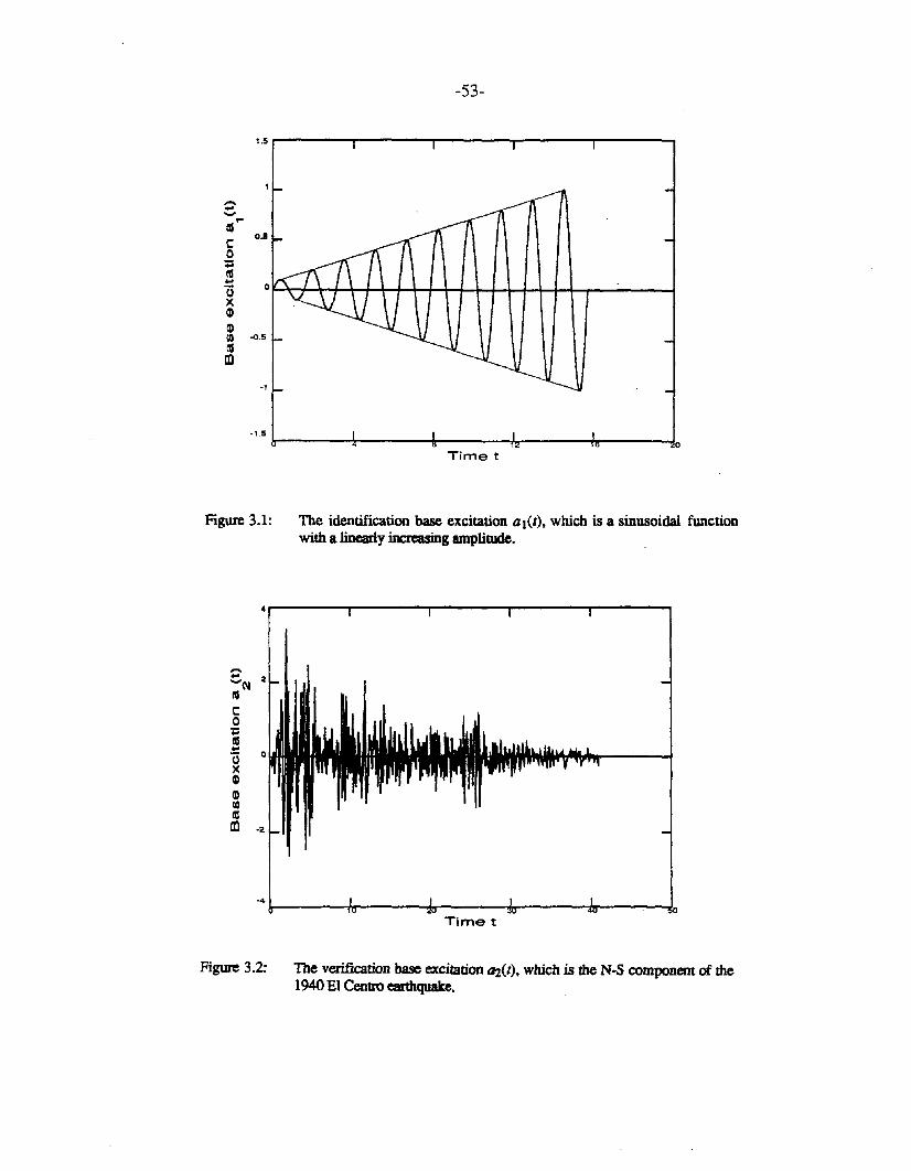
-53-
1.5 r-------r-----r-----"T'""'----r----...,
""".......,1lI'"C
0.-
0..l'G...'0X~
~II) ~.5
tUlD
-1
-1.50
Timet
Figure 3.1: The identification base excitation al(t), which is a sinusoidal functionwith a linearly increasing amplitude.
"""... 2""'(111lIC0..1lI...
0'0X~
~II)
tUlD -2
-4!r-----1l5'----,r----Y-----:r------!oTimet
Figure 3.2: The verification base excitation a,.(t), which is the N-S component of the1940 EI Centro earthquake.
-54-
o.5,..-----...,.------r------r-------,,.-----..,
~'0oi~cQ)
EQ)ocaa.!c
0.25
-<l.25
Displacement---Velocity
-<l.5 Ir------t------ir------~-----.Jr----.....,joTimet
Figure 3.3: The displacement and velocity of the Wen-Boue hysteretic system whensubjected to the identification exeiWion. Qt(t).
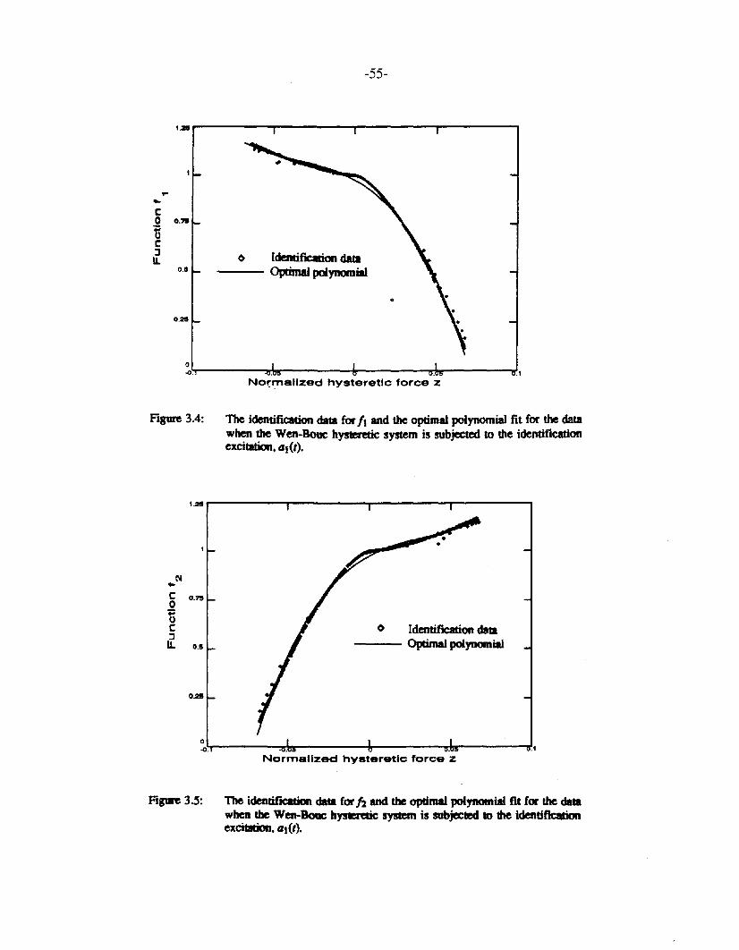
-55-
t.2ll.__----.....----.....,,------...,...-------r
.....co 0.'"
~c:sIL
0.5
0.211
Identification data--- Optimal polynomial
~,l.r.----~r----_lr_----~!lw:_----"'I'I.tNormalized hysteretic force z
Figure 3.4: The identifICation data for /1 and the optimal polynomial fit for the datawhen the Wen-Bouc hysteretic system is subjected to the identificationexcibllion, tJI(t).
t.2Sr------r-----,...------r------,
N...co;::oc:sIL
Identification data--- Optimal polynomial
~". ----......".rM!------+-----~!Ir"----T/..tNormalized hysteretic force z
Figure 3.5: The identifICation data for h and the optimal polynomial fit for the datawhen the Wen-Boac hyseereUc system is subjected to die identificationexcitation, tJI(I).
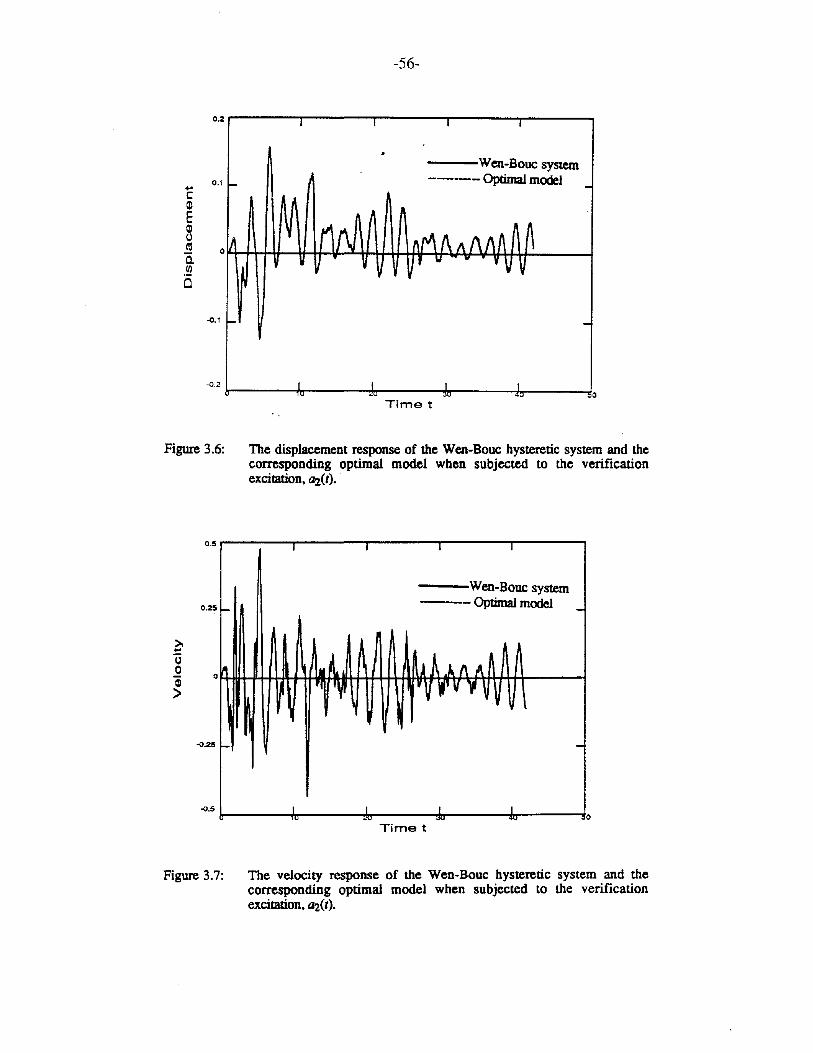
-56-
0.2 r-----r----~---__r----......---__.
...c:QlEQloCO
C.Ul
is
---Wen-Bouc system----- Optimal model
-0.1
-0.2 1r------trJ----r------.j,.,..----~-----.!oTimet
Figure 3.6: The displacement response of the Wen-Boue hysteretic system and thecorresponding optimal model when subjected to the verificationexcitation. a2(t).
0.5
>...."0oQj>
0.25
o
-0.25
-0.5
I I I T
Wen-Boue system
- ---Optimal model -
Ii ~lI
~A A.ll\ A IPI "¥ 1VV W'V 'I \ V,
\
f- -
I I I IlU "'" "'"' 4U 0
Figure 3.7:
Timet
The velocity response of the Wen-Bouc hysteretic system and thecorresponding optimal model when subjected to the verificationexcitation. a2(t).
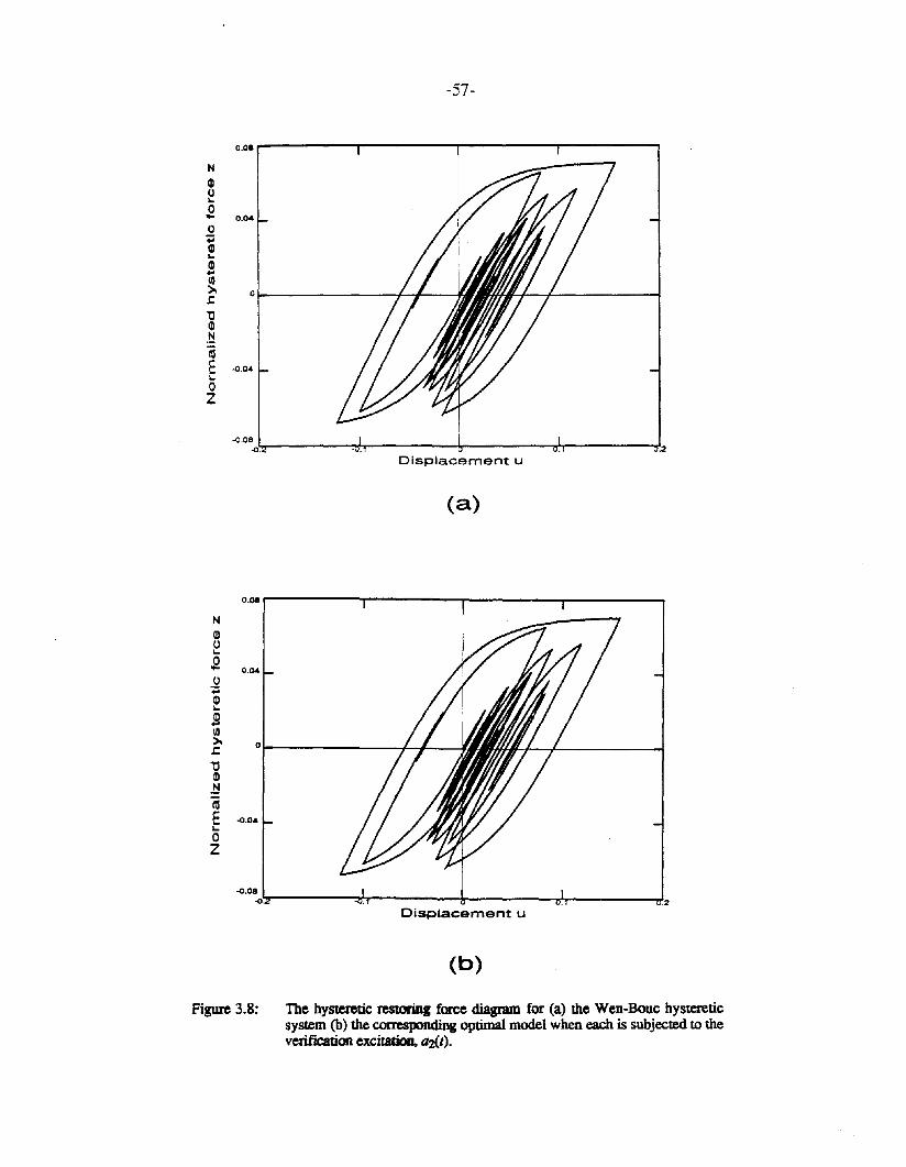
-57-
0.08 ,....-----r--------,r--------.,-------,NQ)
Eo...()..Q)~
!(/)),~
'0Q)
.!:!'iE~
oZ
O.a.
01- -1--1-__
-0.04
-o.08-<)L".-----~-----4------"l,.-----__..,.I.2Displacement u
(a)
0.08 ......------,r---------.-------...-----_
O.a.
01- -1--1-__
-0.04
-o.0~T----_":1!I.r_----__J..__----...,.1...._----...,.J.2
Displacement u
(b)
Figure 3.8: The hysteretic restoring force diagram for (a) the Wen-Bouc hystereticsystem (b) the corresponding optimal model when each is subjected to theverification exciWioo, a'].(t).
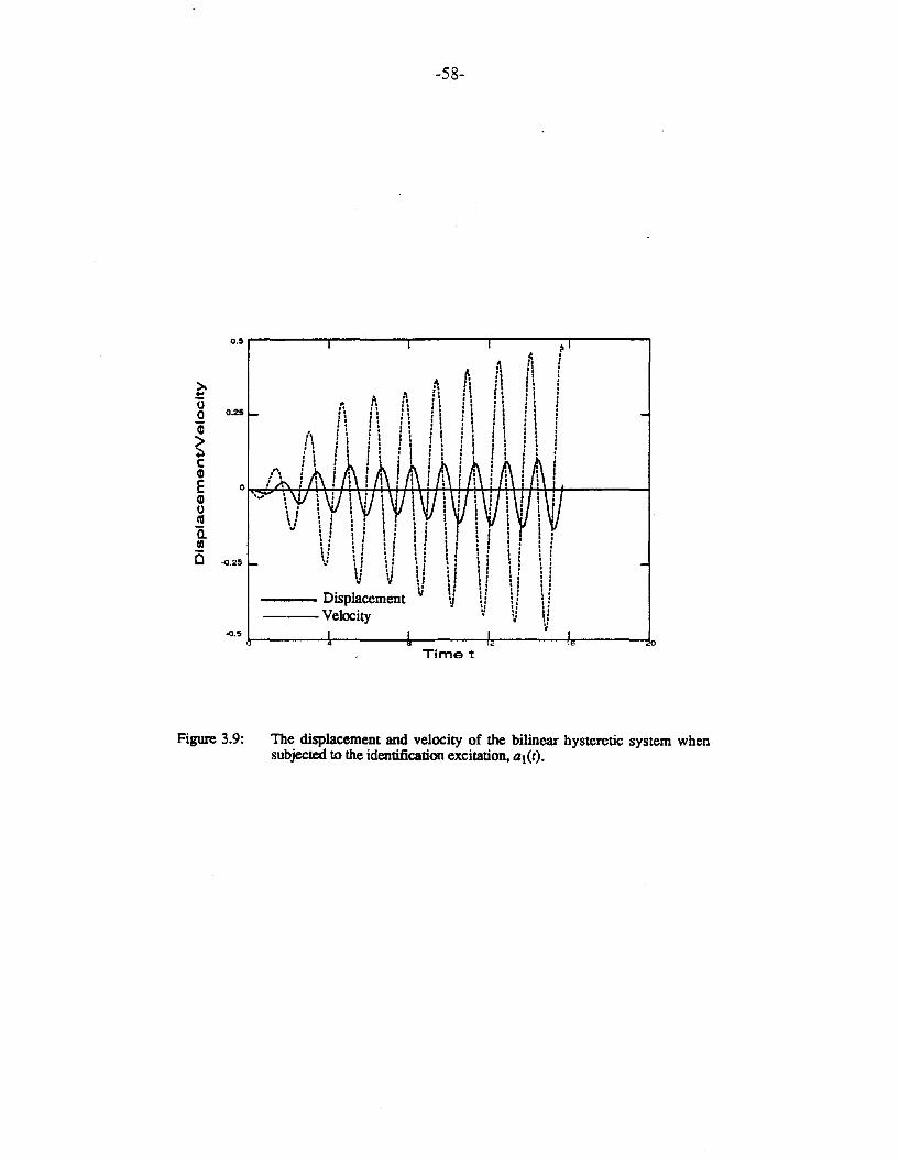
-58-
0.5
A~ \>. 'II, ,... 'I !"0 I,, ,
I0 0.25 : i II
i : i I: I
,
~I
: !I.I, , I
CGlE 0
Gl '"0lU I •a. I, . ,
I ! :.! , ,I ,
!QI I ,• I I-0.25 , I, . ,ij ,
j, ,I,I,
~ '.Displacement 'I'I
" "" "---Velocity " .1
~ ""~-0.5
0
Timet
Figure 3.9: The displacement and velocity of the bilinear hysteretic system whensubjected to the identification excitation, at(t).
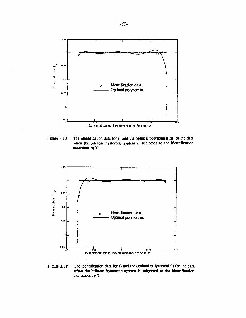
-59-
1.25,.------.--------,...-------,,...-------.,
..-'" 0.75
co';:loC::lU.
0.5
Identif1C8tion data--- Optimal polynomial
•i
.0.25
-<l"T.-------='""',...-----4-------.,.j",.-------..I.1Normalized hysteretic force z
Figure 3.10: The identification data for II and the optimal polynomial fit for the datawhen the bilinear hysteretic system is subjected to the identificationexcitation, QI(t).
1.25 .--------,,...-----_-----.......-----......
0.5
....(11 0.75
Co';:loC::lU.
0.25
o
••
IdentifICation data--- Optimal polynomial
<0.25-<)1,",.-------.,'"'"r------4-------...J.r----~.1Normalized hysteretic force z
Figure 3.11: The identification data forh and the optimal polynomial fit for the datawhen the bilinear hysteretic system is subjected to the identificationexcitation, QI(t).
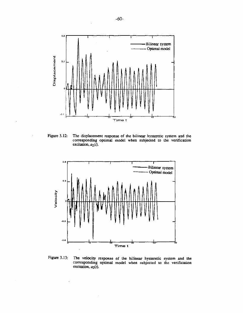
-60-
0.2
<OJ
c:(J) 0.1
E(J)otUa.III
Clo
-0.1
I I I I
Bilinear system------ Optimal model
I'
...• -.
~
~ •~
J" ~"~
~.
• It
~0; t 1~ I
I I I IlU ~u ~u ~u o
Timet
Figure 3.12: The displacement response of the bilinear hysteretic system and thecorresponding optimal model when subjected to the verificationexcitation, a2(t).
o
I I I I
Bilinear system----Optimal model.
~ ~ -• ..
kA
~ ~.
f- -
I I I IlU "'" ~ ..u
o
-0.8
0.8
-0.3
0.3
Timet
Figure 3.13: The velocity response of the bilinear hysteretic system and thecorresponding optimal model when subjected to the verificationexcitation, a2(t).
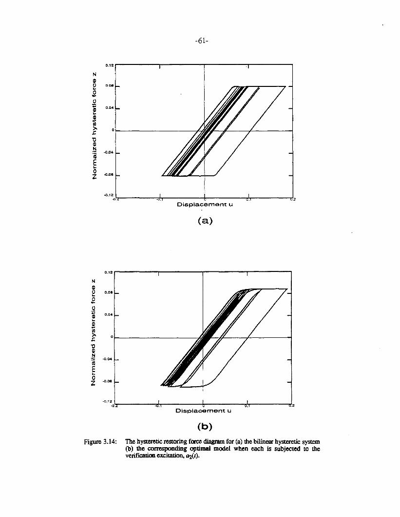
-61-
0.12...------T-------r-------:T"------,
0.08
O.~
0l- ~
-0.08
-o.12-01~.r------:rf,..------!l------'ln-----___rr.2Displacement u
(a)
0.12 ,..-------,------..,...-----...,.------.,
Nal~o...o;;(])...!Ul>J:.iJ(])
~"'iiiE...oZ
0.08
0.04
01- -,
-0.08
-o.1~,L".r------:r+-r-------!Ir-----~n-----___rr.2Displacement u
(b)
Figure 3.14: The hysteretic restoring fm:e diagram for (a) the bilinear hysteretic system(b) the corresponding optimal model when each is subjected to theverification excitation, Q2(t).
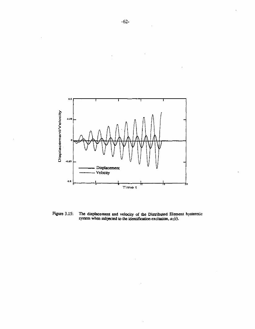
-62-
0.5 ,...-----,.------r-----.,------,-----..,>....'0.2Q)
~c:Q)
EGloraQ.IIIo
0.2!!
-o.2!!
Displacement---Velocity
-o.!! J.-----~.------Ir------.J.r-----1~----~0Timet
Figure 3.15: The displacement and velocity of the Distributed Element hystereticsystem when subjected to the identification excitation. at(t).
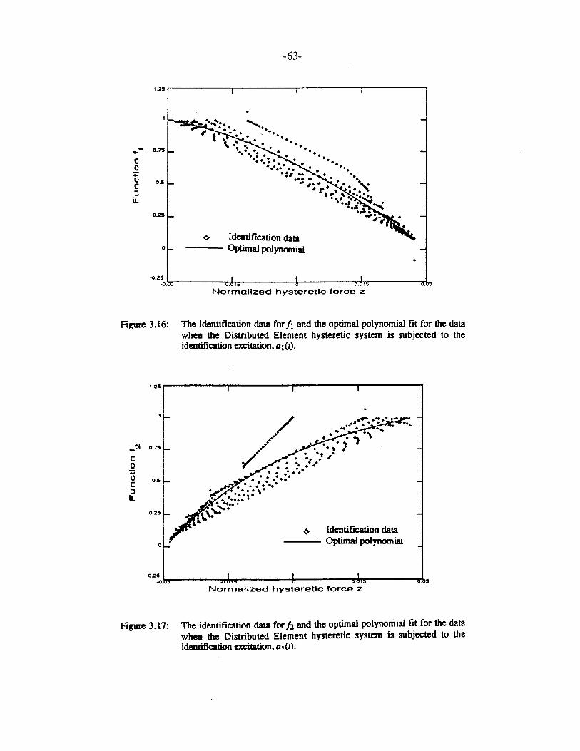
-63-
1.25 r--------r-------.......------..,...------..,
.....c:o;;(,)c:::JU.
o
.. ...••.........
Identification dataOptimal polynomial
-o.2~0.m_-----~h..,..------*_-----_..,h,~----___,..I...3Normalized hysteretic force z
Figure 3.16: The identification data forII and the optimal polynomial fit for the datawhen the Distributed Element hysteretic system is subjected to theidentification excitation, Qt(t).
1.25r-------.,-------"T"------..,..-------,
.3
~ Identiftcation dataOptimal polynomial
./......-/..•....(11 0.75
C0;;(,) 0.5C::JU.
0.25
0
-0.25-0.
Normalized hysteretIc force z
Figure 3.17: The identification data forh and the optimal polynomial fit for the datawhen the Distributed Element hysteretic system is subjected to theidentification excitation, Q1(t).
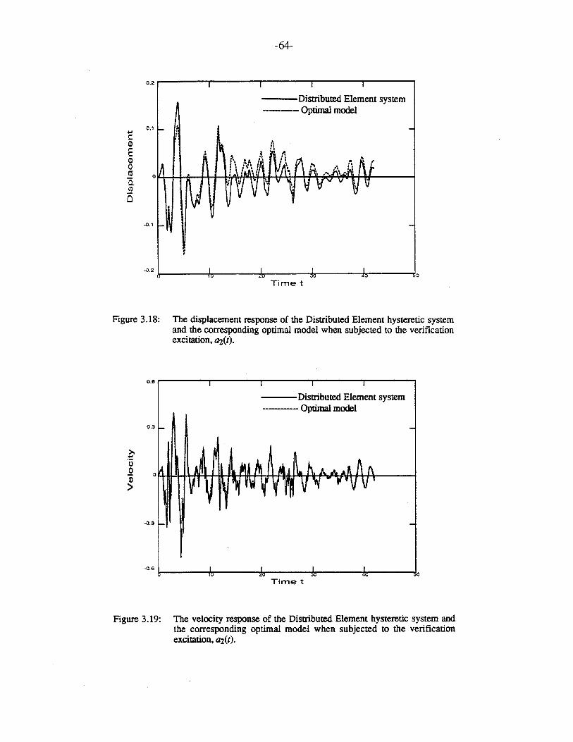
-64-
o.2.-------r----"""T"-----r-----,.-----.....,---Distributed Element system----Optimal model
0.1...CQ)
EalolUC.Ul
Q
-0.2 !<-----+"....-----.m,.----~----:tn-------.!o
Timet
Figure 3.18: The displacement response of the Distributed Element hysteretic systemand the corresponding optimal model when subjected to the verificationexcitation, a2(t).
0.11 r----....,.-----r-----r-----,.-----.....,---Distributed Element system----- Optimal model
0.3
),...'0oQj>
-0.3
-0.6 k----~"...._----o:lrr----~---,._:tn-------.!o
Timet
Figure 3.19: The velocity response of the Distributed Element hysteretic system andthe corresponding optimal model when subjected to the verificationexcitation, a2(t).
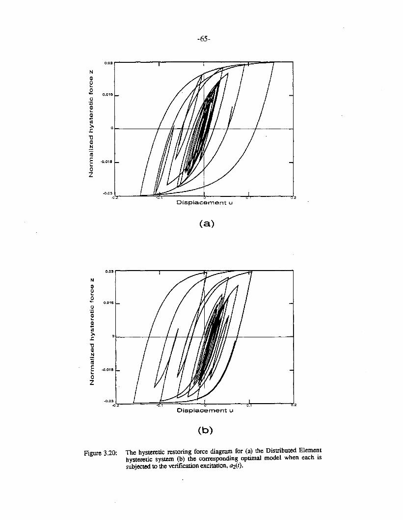
-65-
0.03
NOJ(,)...0.... 0.015(,).;:OJ...OJ...lfl>- 0..c"'0OJ.t:!~E -0.015...0Z
-0.03-{). .2
Displacement u
(a)
NOJeo....(,).;:OJ...OJ...lfl>..c
"'0OJN
~E...oZ
0.03 r----...,-----~::__-=--_=::r_------.
0.015
o1-----1---1:....-,1--1-/---1-
-0.015
-0.03 t--..!====:e:¥======-4r-------Jr-------.J-{)2 2
Displacement u
(b)
Figure 3.20: The hysteretic restoring force diagram for (a) the Distributed Elementhysteretic system (b) the corresponding optimal model when each issubjected to the verification excitation, a2(t).
-66-
CHAPTER 4
COMPARATIVE STUDY OF THE QUASI-STATIC
PERFORMANCE OF TWO HYSTERETIC MODELS
4.1 Introduction:
In Chapter 2, two classes of curvilinear hysteretic models were described. The fIrst is
of the distributed element or assemblage type and the second is of the differential equation
type where one additional state variable is introduced in the formulation along with a fIrst
order, nonlinear differential equation that this state variable satisfIes. The models belonging
to the latter class are also referred to as endochronic models on account of their behavior's
being similar to that of the endochronic models used in plasticity. For this reason, the
second class of models is herein interchangeably referred to as the endochronic class of
hysteretic models.
Certain undesirable behavior exhibited by the endochronic models has been pointed
out previously [24,36,44]. However, Wen, Ang, Baber, Casciyati and others have used
these models extensively for various applications such as:
• Response analysis by the method ofequivalent linearization [10,54],
• Damage evaluation of buildings and the supporting soil systems [54],
• Liquefaction of sand deposits [54],
• System identifIcation of deteriorating systems [46],
• Random vibration of hysteretic systems under bidirectional ground motion [37],
• Nonzero mean random vibrations [5], etc.
The above list is by no means comprehensive: It is given here merely to serve as an
indication of how widely used the endochronic formulation has been in structural
dynamics.
(4.1)
-67-
This chapter performs a comparison of the hysteretic restoring force behavior of the
two classes of curvilinear models by carrying out a set of quasi-static tests. These tests
pertain to cycling between fixed displacement limits as well as cycling between fixed force
limits. This is similar to the cycling of a specimen between fixed strain and stress limits,
respectively, in a physical experiment. The results of these tests show some decidedly
nonphysical behavior on the part of the endochronic models.
In carrying out these analyses, the two models are adjusted to have identical initial
loading curyes so as to facilitate direct comparison. For the Distributed Element model, the
extended Massing's hypothesis formulation is used because of the relative ease of
numerical implementation.
4.2 Hysteretic model representations:
The history dependence of the restoring force behavior of a system is characterized by
the z-u diagrams, where z is the normalized hysteretic force as in Chapter 2 and u is the
displacement of the system. The z-u relationship for various hysteretic models is given in
Chapter 2. In the case of the Wen-Bouc differential equation model, Eqn. (2.38) for n=l,
v=I.0,11=1.0 may be written in the following form:
dz-= A-{3zsgn(du)+ rzdu
where {3, r, A are parameters that control the nature of the hysteretic loops. Given a
variation in u or z, the corresponding variation in the other may be obtained in closed form
by integration of this equation.
In the case of the Distributed Element model in its extended Massing's formulation, z
is obtained by
Z-ZN=<p(U-UN) forN#::O2 2
z =<p(u) for N =0
(4.2.1)
(4.2.2)
-68-
where U ={U1'UZ'U3' ,uNf is an array of N nested turning points which is updated
continuously depending on the history of u in a manner described in Chapter 2 and where
{Zl.ZZ'Z3'•......,zNf is the array of the normalized restoring force values at the
corresponding turning points. Let z=<!J (u) be the initial loading curve for the model. In
order to have the initial loading curve identical to the model in Eqn. (4.1), <!J is defined as
follows:
where
<!J(u) = zy(l-e-u,u,) for u ~ 0
<!J(u) = -¢(-u) for u < 0
Zy =A / (13 - r) , uy=1/(13 - r)
(4.3.1)
(4.3.2)
(4.3.3)
Given a variation in u or z, the corresponding variation in the other may be determined by
means of a simple functional evaluation in Eqn. (4.2).
In all the examples of this chapter, the following values are used for the model
parameters: A=1.0, 13 =0.6, r=-O.4. For these values of the parameters, Zy=uy=1.0. The
initial loading curve has a slope of unity at the origin and rises exponentially to a maximum
or yield value of unity.
The hysteretic energy dissipated by the models, E, is defined as:
E= Jzdu (4.4)
Thus, for a closed loop in the z-u plane, the value of E equals the area enclosed by the
loop.
In what follows, the Wen-Bouc differential equation model is referred to as the W-B
model and the Distributed ELement model with the identical initial loading curve, as the
DEL model.
-69-
4.3 Cyclic loading between fixed displacement limits:
As noted earlier, the cyclic loading of the models between fixed displacement limits
simulates the displacement-controlled testing of the corresponding specimens between fIxed
displacement (or strain) limits in a physical experiment. Two different cases are examined
here, one in which the loading is between symmetric limits and another in which the
loading is between asymmetric limits.
4.3.1 Symmetric cyclic loading:
The following loading sequence is carried out on the two models, which are both
assumed to be in the virgin state: Each model is loaded until the displacement has a value of
1.5, and then is cycled between the displacement values of 1.5 and -1.5.
Fig. 4.1 shows the manner in which the normalized restoring force, z, of the two
hysteretic models behaves for this loading pattern. The following remarks can be made
regarding the hysteretic behavior of the two models:
(1) From Fig. 4.1a, it is seen that the DEL model settles to a stable, closed loop after just
one load cycle. In the case of the W-B model, since the system returns to 3 instead of to
1 after one cycle, there is a nonclosure of the loop. However, after one more cycle, the
loop is essentially closed. For further cycling, the system settles to the stable loop 343.
Thus, for displacement loading between fIxed symmetric limits, the W-B model
exhibits curvilinear, closed hysteresis loops in the steady state.
(2)Unlike the case of the DEL model, it may be noted that the turning points of the stable
loop for the W-B model do not lie on the initial loading curve. For cyclic loading
between the displacement limits ±uA , the normalized restoring force values
corresponding to the turning points of the stable cycle, ±ZA' can be shown to satisfy
the equation
-70-
1 z 1 z--log[1+...a(/3 + r)] - log[1-...a(/3 - r)] for r #: 13(13 +r) A (13 - r) A
1 I 213 ZA z~ & 13- og[1+ -]+- lorr=213 A A
(4.5)
Let the locus of points, (UA,ZA)' be defined to be the turning point curve for the W-B
hysteretic model, with an odd extension being made about the origin as in the case of
the initial loading curve. The turning points or the load reversal points of the W-B
model for cycling between fixed, symmetric displacement limits lie on the turning point
curve in the steady state. As uA becomes very large, the turning point curve tends to Zy'
the same value as the initial loading curve. The turning point curve for A=l.O, 13 =0.6,
r =-0.4, is shown in Fig. 4.1b.
(3) It can be seen that the W-B model exhibits a stiffness-increase or stiffening, which is
apparent from the rotation of the initial loops to a stiffer stable loop. Such a stiffening
feature is not present in the DEL model. Thus, for the same displacement, the W-B
model has a larger effective stiffness than the DEL model. This stiffening occurs for the
the W-B model for all values of 13 and r, that is, for both softening and hardening
systems. This claim can be verified in the following fashion. The slope of the initial
loading curve satisfies
dz- = A - z(/3 - r)du
(4.6.1)
By differentiating Eqn. (4.5), the following expression can be obtained for the slope of
the turning point curve:
dz 2-= A+zr+O(z )du
(4.6.2)
At z=O, the slopes of both curves is A. For very small values of z, the turning point
curve has a slope larger then the initial loading curve if 13 >0. The condition 13 >0 is
essential in the W-B model because it alone ensures that the unloading stiffness is larger
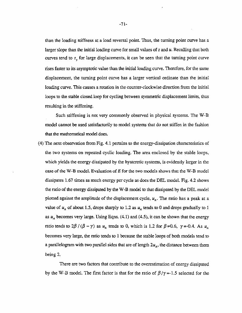
-71-
than the loading stiffness at a load reversal point. Thus, the turning point curve has a
larger slope than the initial loading curve for small values of z and u. Recalling that both
curves tend to Zy for large displacements, it can be seen that the turning point curve
rises faster to its asymptotic value than the initial loading curve. Therefore, for the same
displacement, the turning point curve has a larger vertical ordinate than the initial
loading curve. This causes a rotation in the counter-clockwise direction from the initial
loops to the stable closed loop for cycling between symmetric displacement limits, thus
resulting in the stiffening.
Such stiffening is not very commonly observed in physical systems. The W-B
model cannot be used satisfactorily to model systems that do not stiffen in the fashion
that the mathematical model does.
(4) The next observation from Fig. 4.1 pertains to the energy-dissipation characteristics of
the two systems on repeated cyclic loading. The area enclosed by the stable loops,
which yields the energy dissipated by the hysteretic systems, is evidently larger in the
case of the W-B model. Evaluation of E for the two models shows that the W-B model
dissipates 1.67 times as much energy per cycle as does the DEL model. Fig. 4.2 shows
the ratio of the energy dissipated by the W-B model to that dissipated by the DEL model
plotted against the amplitude of the displacement cycle, uA • The ratio has a peak at a
value of uA of about 1.5, drops sharply to 1.2 as uA tends to 0 and drops gradually to 1
as uA becomes very large. Using Eqns. (4.1) and (4.5), it can be shown that the energy
ratio tends to 2f3 / (f3 - r) as uA tends to 0, which is 1.2 for f3 =0.6, r =-0.4. As uA
becomes very large, the ratio tends to 1 because the stable loops of both models tend to
a parallelogram with two parallel sides that are of length 2uA , the distance between them
being 2.
There are two factors that contribute to the overestimation of energy dissipated
by the W-B model. The fIrst factor is that for the ratio of f3 / r =-1.5 selected for the
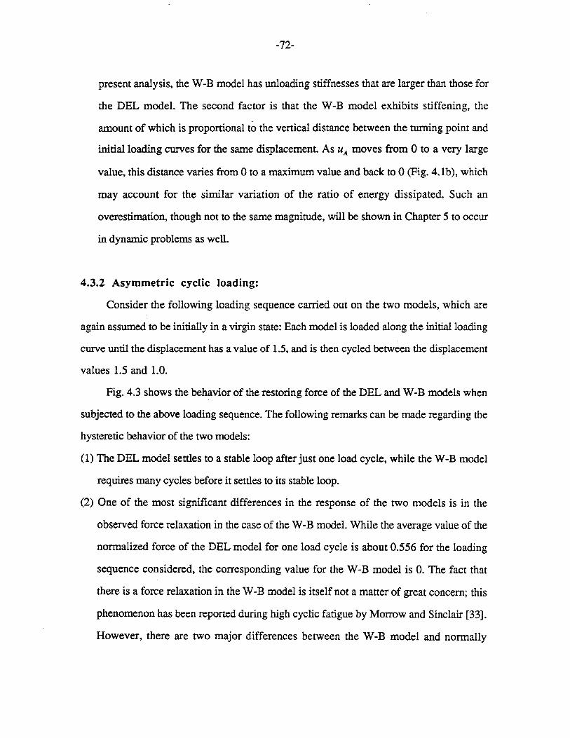
-72-
present analysis, the W-B model has unloading stiffnesses that are larger than those for
the DEL model. The second factor is that the W-B model exhibits stiffening, the
amount of which is proportional to the vertical distance between the turning point and
initial loading curves for the same displacement. As UA moves from 0 to a very large
value, this distance varies from 0 to a maximum value and back to 0 (Fig. 4.1b), which
may account for the similar variation of the ratio of energy dissipated. Such an
overestimation, though not to the same magnitude, will be shown in Chapter 5 to occur
in dynamic problems as well.
4.3.2 Asymmetric cyclic loading:
Consider the following loading sequence carried out on the two models, which are
again assumed to be initially in a virgin state: Each model is loaded along the initial loading
curve until the displacement has a value of 1.5, and is then cycled between the displacement
values 1.5 and 1.0.
Fig. 4.3 shows the behavior of the restoring force of the DEL and W-B models when
subjected to the above loading sequence. The following remarks can be made regarding the
hysteretic behavior of the two models:
(1) The DEL model settles to a stable loop after just one load cycle, while the W-B model
requires many cycles before it settles to its stable loop.
(2) One of the most significant differences in the response of the two models is in the
observed force relaxation in the case of the W-B model. While the average value of the
normalized force of the DEL model for one load cycle is about 0.556 for the loading
sequence considered, the corresponding value for the W-B model is O. The fact that
there is a force relaxation in the W-B model is itself not a matter of great concern; this
phenomenon has been reported during high cyclic fatigue by Morrow and Sinclair [33].
However, there are two major differences between the W-B model and normally
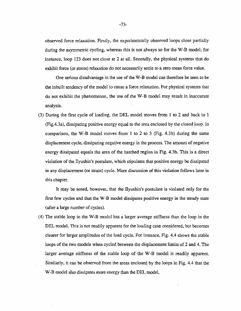
-73-
observed force relaxation. Firstly, the experimentally observed loops close partiaJly
during the asymmetric cycling, whereas this is not always so for the W-B model; for
instance, loop 123 does not close at 2 at all. Secondly, the physical systems that do
exhibit force (or stress) relaxation do not necessarily settle to a zero mean force value.
One serious disadvantage in the use of the W-B model can therefore be seen to be
the inbuilt tendency of the model to cause a force relaxation. For physical systems that
do not exhibit the phenomenon, the use of the W-B model may result in inaccurate
analysis.
(3) During the fIrst cycle of loading, the DEL model moves from 1 to 2 and back to 1
(Fig.4.3a), dissipating positive energy equal to the area enclosed by the closed loop. In
comparison, the W-B model moves from 1 to 2 to 3 (Fig. 4.3b) during the same
displacement cycle, dissipating negative energy in the process. The amount of negative
energy dissipated equals the area of the hatched region in Fig. 4.3b. This is a direct
violation of the Ilyushin's postulate, which stipulates that positive energy be dissipated
in any displacement (or strain) cycle. More discussion of this violation follows later in
this chapter.
It may be noted, however, that the Ilyushin's postulate is violated only for the
fIrst few cycles and that the W-B model dissipates positive energy in the steady state
(after a large number of cycles).
(4) The stable loop in the W-B model has a larger average stiffness than the loop in the
DEL model. This is not readily apparent for the loading case considered, but becomes
clearer for larger amplitudes of the load cycle. For instance, Fig. 4.4 shows the stable
loops of the two models when cycled between the displacement limits of 2 and 4. The
larger average stiffness of the stable loop of the W-B model is readily apparent.
Similarly, it can be observed from the areas enclosed by the loops in Fig. 4.4 that the
W-B model also dissipates more energy than the DEL model.
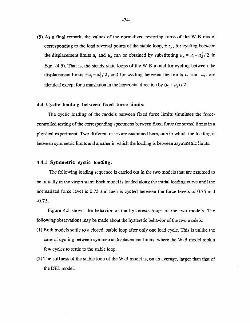
-74-
(5) As a final remark, the values of the normalized restoring force of the W-B model
corresponding to the load reversal points of the stable loop, ± ZA' for cycling between
the displacement limits ~ and u;, can be obtained by substituting uA = I~ - ~I /2 in
Eqn. (4.5). That is, the steady-state loops of the W-B model for cycling between the
displacement limits ±I~ - ~1/2, and for cycling between the limits ~ and ~, are
identical except for a translation in the horizontal direction by (~ +~) / 2.
4.4 Cyclic loading between fixed force limits:
The cyclic loading of the models between fixed force limits simulates the force
controlled testing of the corresponding specimens between fixed force (or stress) limits in a
physical experiment. Two different cases are examined here, one in which the loading is
between symmetric limits and another in which the loading is between asymmetric limits.
4.4.1 Symmetric cyclic loading:
The following loading sequence is carried out in the two models that are assumed to
be initially in the virgin state: Each model is loaded along the initial loading curve until the
normalized force level is 0.75 and then is cycled between the force levels of 0.75 and
-0.75.
Figure 4.5 shows the behavior of the hysteresis loops of the two models. The
following observations may be made about the hysteretic behavior of the two models:
(1) Both models settle to a closed, stable loop after only one load cycle. This is unlike the
case of cycling between symmetric displacement limits, where the W-B model took a
few cycles to settle to the stable loop.
(2) The stiffness of the stable loop of the W-B model is, on an average, larger than that of
the DEL model.
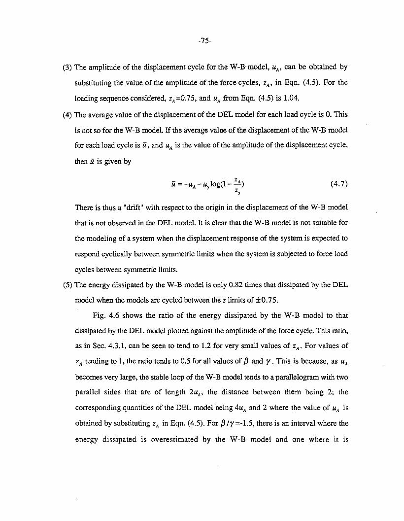
-75-
(3) The amplitude of the displacement cycle for the W-Rmodel, uA ' can be obtained by
substituting the value of the amplitude of the force cycles, ZA' in Eqn. (4.5). For the
loading sequence considered, ZA =0.75, and uA from Eqn. (4.5) is 1.04.
(4) The average value of the displacement of the DEL model for each load cycle is O. This
is not so for the W-B model. If the average value of the displacement of the W-B model
for each load cycle is it, and uA is the value of the amplitude of the displacement cycle,
then it is given by
(4.7)
There is thus a "drift" with respect to the origin in the displacement of the W-B model
that is not observed in the DEL model. It is clear that the W-B model is not suitable for
the modeling of a system when the displacement response of the system is expected to
respond cyclically between symmetric limits when the system is subjected to force load
cycles between symmetric limits.
(5) The energy dissipated by the W-B model is only 0.82 times that dissipated by the DEL
model when the models are cycled between the Z limits of ±0.75.
Fig. 4.6 shows the ratio of the energy dissipated by the W-B model to that
dissipated by the DEL model plotted against the amplitude of the force cycle. This ratio,
as in Sec. 4.3.1, can be seen to tend to 1.2 for very small values of ZA. For values of
ZA tending to 1, the ratio tends to 0.5 for all values of f3 and r. This is because, as uA
becomes very large, the stable loop of the W-B model tends to a parallelogram with two
parallel sides that are of length 2uA , the distance between them being 2; the
corresponding quantities of the DEL model being 4uA and 2 where the value of uA is
obtained by substituting ZA in Eqn. (4.5). For f3 /r =-1.5, there is an interval where the
energy dissipated is overestimated by the W-B model and one where it is
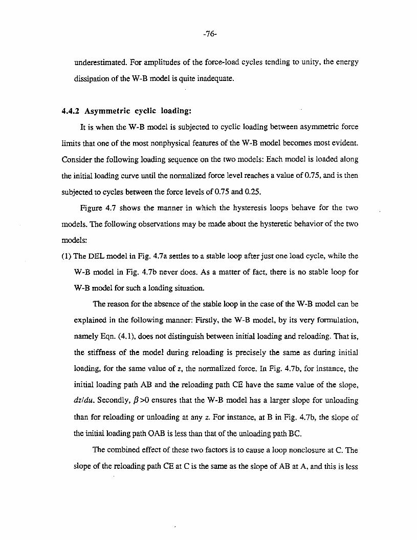
-76-
underestimated. For amplitudes of the force-load cycles tending to unity, the energy
dissipation of the W-B model is quite inadequate.
4.4.2 Asymmetric cyclic loading:
It is when the W-B model is subjected to cyclic loading between asymmetric force
limits that one of the most nonphysical features of the W-B model becomes most evident.
Consider the following loading sequence on the two models: Each model is loaded along
the initial loading curve until the normalized force level reaches a value of 0.75, and is then
subjected to cycles between the force levels of 0.75 and 0.25.
Figure 4.7 shows the manner in which the hysteresis loops behave for the two
models. The following observations may be made about the hysteretic behavior of the two
models:
(1) The DEL model in Fig. 4.7a settles to a stable loop after just one load cycle, while the
W-B model in Fig. 4.7b never does. As a matter of fact, there is no stable loop for
W-B model for such a loading situation.
The reason for the absence of the stable loop in the case of the W-B model can be
explained in the following manner: Firstly, the W-B model, by its very formulation,
namely Eqn. (4.1), does not distinguish between initial loading and reloading. That is,
the stiffness of the model during reloading is precisely the same as during initial
loading, for the same value of z, the normalized force. In Fig. 4.7b, for instance, the
initial loading path AB and the reloading path CE have the same value of the slope,
dz!duo Secondly, f3 >0 ensures that the W-B model has a larger slope for unloading
than for reloading or unloading at any z. For instance, at B in Fig. 4.7b, the slope of
the initial loading path GAB is less than that of the unloading path BC.
The combined effect of these two factors is to cause a loop nonclosure at C. The
slope of the reloading path CE at C is the same as the slope of AB at A, and this is less
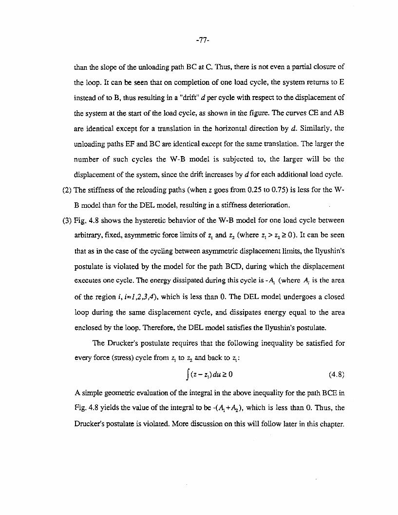
-77-
than the slope of the unloading path BC at C. Thus, there is not even a partial closure of
the loop. It can be seen that on completion of one load cycle, the system returns to E
instead of to B, thus resulting in a "drift" d per cycle with respect to the displacement of
the system at the start of the load cycle, as shown in the figure. The curves CE and AB
are identical except for a translation in the horizontal direction by d. Similarly, the
unloading paths EF and BC are identical except for the same translation. The larger the
number of such cycles the W-B model is subjected to, the larger will be the
displacement of the system, since the drift increases by d for each additional load cycle.
(2) The stiffness of the reloading paths (when Z goes from 0.25 to 0.75) is less for the W
B model than for the DEL model, resulting in a stiffness deterioration.
(3) Fig. 4.8 shows the hysteretic behavior of the W-B model for one load cycle between
arbitrary, fixed, asymmetric force limits of Zl and Zz (where Zl> Zz ~ 0). It can be seen
that as in the case of the cycling between asymmetric displacement limits, the Ilyushin's
postulate is violated by the model for the path BCD, during which the displacement
executes one cycle. The energy dissipated during this cycle is -AI (where ~ is the area
of the region i, i=],2,3 ,4), which is less than O. The DEL model undergoes a closed
loop during the same displacement cycle, and dissipates energy equal to the area
enclosed by the loop. Therefore, the DEL model satisfies the ilyushin's postulate.
The Drucker's postulate requires that the following inequality be satisfied for
every force (stress) cycle from Zl to Zz and back to Zl:
f(Z-ZI)du~O (4.8)
A simple geometric evaluation of the integral in the above inequality for the path BCE in
Fig. 4.8 yields the value of the integral to be -(AI +Az), which is less than O. Thus, the
Drucker's postulate is violated. More discussion on this will follow later in this chapter.
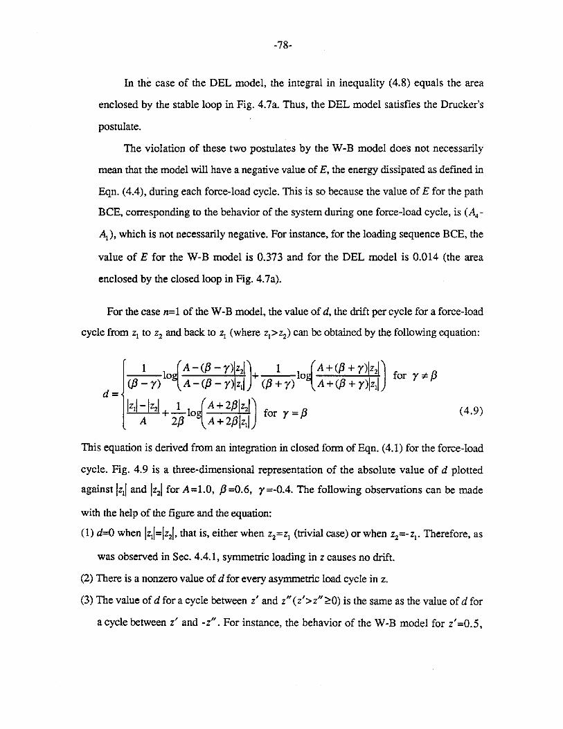
-78-
In the case of the DEL model, the integral in inequality (4.8) equals the area
enclosed by the stable loop in Fig. 4.7a. Thus, the DEL model satisfies the Drucker's
postulate.
The violation of these two postulates by the W-B model does not necessarily
mean that the model will have a negative value of E, the energy dissipated as defmed in
Eqn. (4.4), during each force-load cycle. This is so because the value of E for the path
BCE, corresponding to the behavior of the system during one force-load cycle, is (A4
AI)' which is not necessarily negative. For instance, for the loading sequence BCE, the
value of E for the W-B model is 0.373 and for the DEL model is 0.014 (the area
enclosed by the closed loop in Fig. 4.7a).
For the case n=1 of the W-B model, the value of d, the drift per cycle for a force-load
cycle from Zl to Z2 and back to Zl (where ZI>Z2) can be obtained by the following equation:
d=
(4.9)
This equation is derived from an integration in closed form of Eqn. (4.1) for the force-load
cycle. Fig. 4.9 is a three-dimensional representation of the absolute value of d plotted
against IZII and IZ21 for A=1.0, /3=0.6, r=-O.4. The following observations can be made
with the help of the figure and the equation:
(1) d=O when IZII=lz2/' that is, either when Z2=ZI (trivial case) or when Z2=-ZI' Therefore, as
was observed in Sec. 4.4.1, symmetric loading in Z causes no drift.
(2) There is a nonzero value of d for every asymmetric load cycle in z.
(3) The value of d for a cycle between z' and z" (z'> z" ~O) is the same as the value of d for
a cycle between z' and -z". For instance, the behavior of the W-B model for z'=0.5,
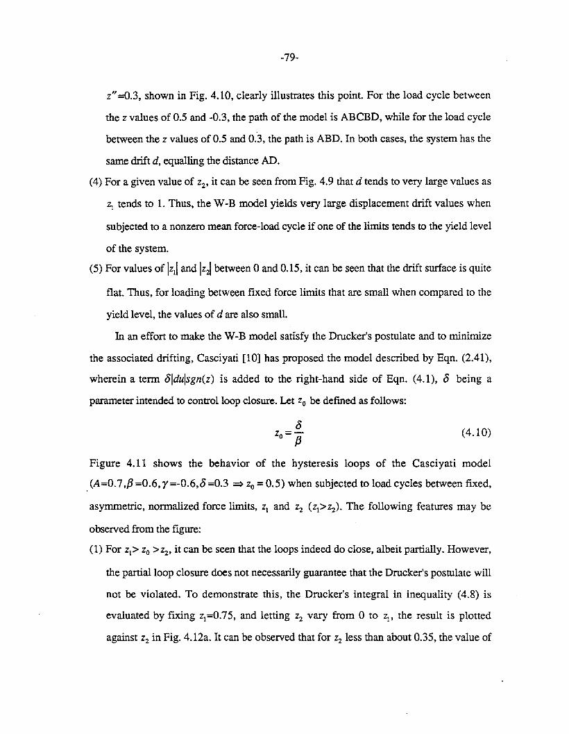
-79-
z"=0.3, shown in Fig. 4.10, clearly illustrates this point. For the load cycle between
the z values of 0.5 and -0.3, the path of the model is ABCBD, while for the load cycle
between the z values of 0.5 and 0.3, the path is ABD. In both cases, the system has the
same drift d, equalling the distance AD.
(4) For a given value of Z2' it can be seen from Fig. 4.9 that d tends to very large values as
Z1 tends to 1. Thus, the W-B model yields very large displacement drift values when
subjected to a nonzero mean force-load cycle if one of the limits tends to the yield level
of the system.
(5) For values of IZll and Iz~ between 0 and 0.15, it can be seen that the drift surface is quite
flat. Thus, for loading between fixed force limits that are small when compared to the
yield level, the values of d are also small.
In an effort to make the W-B model satisfy the Drucker's postulate and to minimize
the associated drifting, Casciyati [10] has proposed the model described by Eqn. (2.41),
wherein a term 8Idulsgn(z) is added to the right-hand side of Eqn. (4.1), 8 being a
parameter intended to control loop closure. Let Zo be defined as follows:
8z=-o /3 (4.10)
Figure 4.11 shows the behavior of the hysteresis loops of the Casciyati model
(A=0.7,/3 =0.6, r=-0.6,8 =0.3 => Zo = 0.5) when subjected to load cycles between fixed,
asymmetric, normalized force limits, Z1 and Z2 (Z1>Z2)' The following features may be
observed from the figure:
(1) For Z1> Zo >Z2' it can be seen that the loops indeed do close, albeit partially. However,
the partial loop closure does not necessarily guarantee that the Drucker's postulate will
not be violated. To demonstrate this, the Drucker's integral in inequality (4.8) is
evaluated by fixing zl=0.75, and letting Z2 vary from 0 to zl' the result is plotted
against Z2 in Fig. 4.12a. It can be observed that for Z2 less than about 0.35, the value of
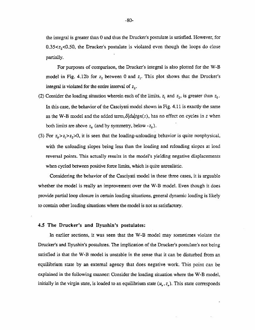
-80-
the integral is greater than °and thus the Drucker's postulate is satisfied. However, for
0.35<zz<0.50, the Drucker's postulate is violated even though the loops do close
partially.
For purposes of comparison, the Drucker's integral is also plotted for the W-B
model in Fig. 4.12b for Zz between °and Zl' This plot shows that the Drucker's
integral is violated for the entire interval of zz.
(2) Consider the loading situation wherein each of the limits, Zl and zz' is greater than zo'
In this case, the behavior of the Casciyati model shown in Fig. 4.11 is exactly the same
as the W-B model and the added term,8Idulsgn(z) , has no effect on cycles in Z when
both limits are above Zo (and by symmetry, below -zo)'
(3) For ZO>Zl>ZZ>O, it is seen that the loading-unloading behavior is quite nonphysical,
with the unloading slopes being less than the loading and reloading slopes at load
reversal points. This actually results in the model's yielding negative displacements
when cycled between positive force limits, which is quite unrealistic.
Considering the behavior of the Casciyati model in these three cases, it is arguable
whether the model is really an improvement over the W-B model. Even though it does
provide partial loop closure in certain loading situations, general dynamic loading is likely
to contain other loading situations where the model is not as satisfactory.
4.5 The Drucker's and Ilyushin's postulates:
In earlier sections, it was seen that the W-B model may sometimes violate the
Drucker's and Ilyushin's postulates. The implication of the Drucker's postulate's not being
satisfied is that the W-B model is unstable in the sense that it can be disturbed from an
equilibrium state by an external agency that does negative work. This point can be
explained in the following manner: Consider the loading situation where the W-B model,
initially in the virgin state, is loaded to an equilibrium state (ue, ze)' This state corresponds
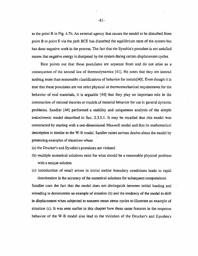
-81-
to the point B in Fig. 4.7b. An external agency that causes the model to be disturbed from
point B to point E via the path BeE has disturbed the equilibrium state of the system but
has done negative work in the process. The fact that the ilyushin's postulate is not satisfied
means that negative energy is dissipated by the system during certain displacement cycles.
Rice points out that these postulates are separate from and do not arise as a
consequence of the second law of thermodynamics [41]. He notes that they are instead
nothing more than reasonable classifications of behavior for metals[40]. Even though it is
true that these postulates are not strict physical or thermomechanical requirements for the
behavior of real materials, it is arguable [44] that they play an important role in the
construction of rational theories or models of material behavior for use in general dynamic
problems. Sandler [44] performed a stability and uniqueness analysis of the simple
endochronic model described in Sec. 2.3.5.1. It may be recalled that this model was
constructed by starting with a one-dimensional Maxwell model and that its mathematical
description is similar to the W-B model. Sandler raises serious doubts about the model by
presenting examples of situations where
(a) the Drucker's and ilyushin's postulates are violated
(b) multiple numerical solutions exist for what should be a reasonable physical problem
with a unique solution
(c) introduction of small errors in initial and/or boundary conditions leads to rapid
deterioration in the accuracy of the numerical solutions for subsequent computations.
Sandler uses the fact that the model does not distinguish between initial loading and
reloading to demonstrate an example of situation (b) and the tendency of the model to drift
in displacement when subjected to nonzero mean stress cycles to illustrate an example of
situation (c). It was seen earlier in this chapter how these same features in the response
behavior of the W-B model also lead to the violation of the Drucker's and Ilyushin's
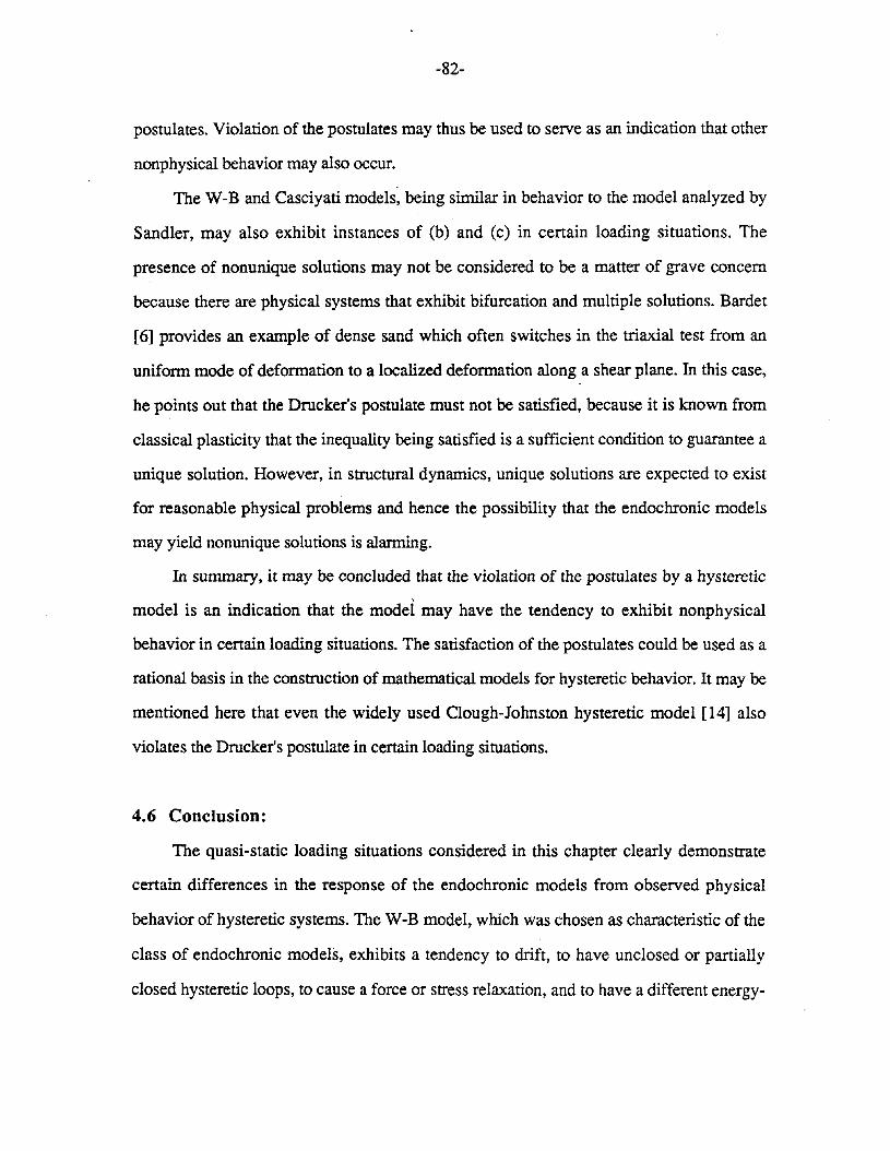
-82-
postulates. Violation of the postulates may thus be used to serve as an indication that other
nonphysical behavior may also occur.
The W-B and Casciyati models, being similar in behavior to the model analyzed by
Sandler, may also exhibit instances of (b) and (c) in certain loading situations. The
presence of nonunique solutions may not be considered to be a matter of grave concern
because there are physical systems that exhibit bifurcation and multiple solutions. Bardet
[6] provides an example of dense sand which often switches in the triaxial test from an
uniform mode of deformation to a localized deformation along a shear plane. In this case,
he points out that the Drucker's postulate must not be satisfied, because it is known from
classical plasticity that the inequality being satisfied is a sufficient condition to guarantee a
unique solution. However, in structural dynamics, unique solutions are expected to exist
for reasonable physical problems and hence the possibility that the endochronic models
may yield nonunique solutions is alarming.
In summary, it may be concluded that the violation of the postulates by a hysteretic
model is an indication that the model may have the tendency to exhibit nonphysical
behavior in certain loading situations. The satisfaction of the postulates could be used as a
rational basis in the construction of mathematical models for hysteretic behavior. It may be
mentioned here that even the widely used Clough-Johnston hysteretic model [14] also
violates the Drucker's postulate in certain loading situations.
4.6 Conclusion:
The quasi-static loading situations considered in this chapter clearly demonstrate
certain differences in the response of the endochronic models from observed physical
behavior of hysteretic systems. The W-B model, which was chosen as characteristic of the
class of endochronic models, exhibits a tendency to drift, to have unclosed or partially
closed hysteretic loops, to cause a force or stress relaxation, and to have a different energy-
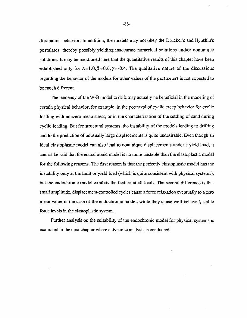
-83-
dissipation behavior. In addition, the models may not obey the Drucker's and Ilyushin's
postulates, thereby possibly yielding inaccurate numerical solutions and/or nonunique
solutions. It may be mentioned here that the quantitative results of this chapter have been
established only for A=l.O,,B =0.6, r=-OA. The qualitative nature of the discussions
regarding the behavior of the models for other values of the parameters is not expected to
be much different.
The tendency of the W-B model to drift may actually be beneficial in the modeling of
certain physical behavior, for example, in the portrayal of cyclic creep behavior for cyclic
loading with nonzero mean stress, or in the characterization of the settling of sand during
cyclic loading. But for structural systems, the instability of the models leading to drifting
and to the prediction of unusually large displacements is quite undesirable. Even though an
ideal elastoplastic model can also lead to nonunique displacements under a yield load, it
cannot be said that the endochronic model is no more unstable than the elastoplastic model
for the following reasons. The first reason is that the perfectly elastoplastic model has the
instability only at the limit or yield load (which is quite consistent with physical systems),
but the endochronic model exhibits the feature at all loads. The second difference is that
small amplitude, displacement-controlled cycles cause a force relaxation eventually to a zero
mean value in the case of the endochronic model, while they cause well-behaved, stable
force levels in the elastoplastic system.
Further analysis on the suitability of the endochronic model for physical systems is
examined in the next chapter where a dynamic analysis is conducted.
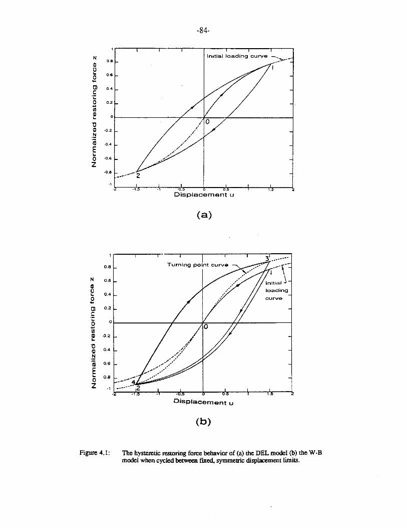
-84-
N0.8
(])0~ 0.60...Cl 0.4c:~0 0.2...Ul(])
0~
'C(]) ·0.2
.~
iii -0.4
E~
0 -0.6
Z-0.8 _-_.-.- 2
·1.1.
0.8
N 0.6(])0
0.4~
0...Cl 0.2
c:'i: a0...Ul(]) ·0.2~
'C0.4(])
.~
iii 0.6
E~ 0.80Z
Initial loading curve
·1
Displacement u
(a)
3 ._.\-In1itial
loading
curve
Displacement u
(b)
Figure 4.1: The hysteretic restoring force behavior of (a) the DEL model (b) the W-Bmodel when cycled between fIXed, symmetric displacement limits.
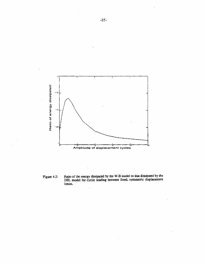
-85-
"0Q)
m1.75a.
"Ui(/l
'6>.Cl..Q) 1.5
c:Q)...00"';:t1l 1.25
ct
Figure 4.2:
1r----.....;----+----J~---__f,,---_J5Amplitude of displacement cycles
Ratio of the energy dissipated by the W-B model to that dissipated by theDEL model for cyclic loading between fixed. symmetric displacementlimits.
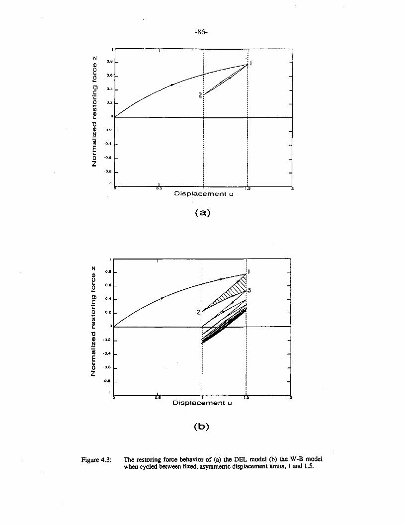
-86-
N0.8
OJ0~ 0.60...OJ 0.4c::.~
0 0.2...enQ)
0~
'CQ) ·0.2
.~(ij -0.4
E~
0 -0.6
Z-0.8
-1
1 1.
Displacement u
(a)
NQ)
eo...OJc::.~
o...enQ)~
'CQ)
.~(ijE~
oZ
-0.6
-0.8
-1 /r------7fT:-------1--------;.!r-------l,Displacement u
(b)
Figure 4.3: The restoring force behavior of (a) the DEL model (b) the W-B modelwhen cycled between fixed, asymmetric displacement limits, 1 and 1.5.
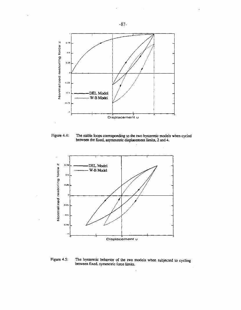
N 0.75
OJU...0 0.5....OJC'i: 0.25
0...CJ)
OJ 0...'0OJN -0.25
(ijE... ·0.50Z
-0.75
.,
Figure 4.4:
N 0.75
(J)(J...0 0.5....OJC'i: 0.25
0Cii(J)
0...'0Q)N ·0.25
(ijE... -0.50Z
-0.75
.,
Figure 4.5:
-87-
~---DELModel---W-B Model
Displacement u
The stable loops corresponding to the two hysteretic models when cycledbetween the fIxed, asymmetric displacement limits, 2 and 4.
---DEL Model,---W-B Model
Displacement u
The hysteretic behavior of the two models when subjected to cyclingbetween fIxed, symmetric force limits.
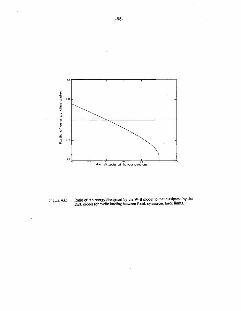
-88-
1.5
iJQl'iii
1.25a.'(jjUliJ>,OJ....QlcQl...00+:ctl 0.75
[
05k---~...-- .2
Amplitude of force cycles
Figure 4.6: Ratio of the energy dissipated by the W-B model to that dissipated by theDEL model for cyclic loading between fIxed, symmetric force limits.
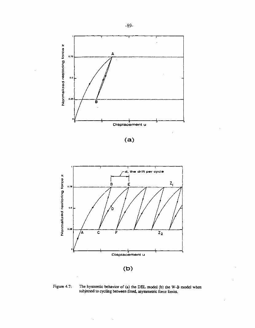
NQ)
eo 0.75~
Clc:'t:o...(/)
~ 0.5
'0Q)N
iE..oZ
N
al~o 0.75~
Clc:.~
o..en~ 0.5
'0alN
iE..oZ
Figure 4.7:
-89-
A
Displacement u
(a)
H the drift per cycle
B E Z,
Displacement u
(b)
The hysteretic behavior of (a) the DEL model (b) the W-B model whensubjected to cycling between fIxed, asymmetric force limits.
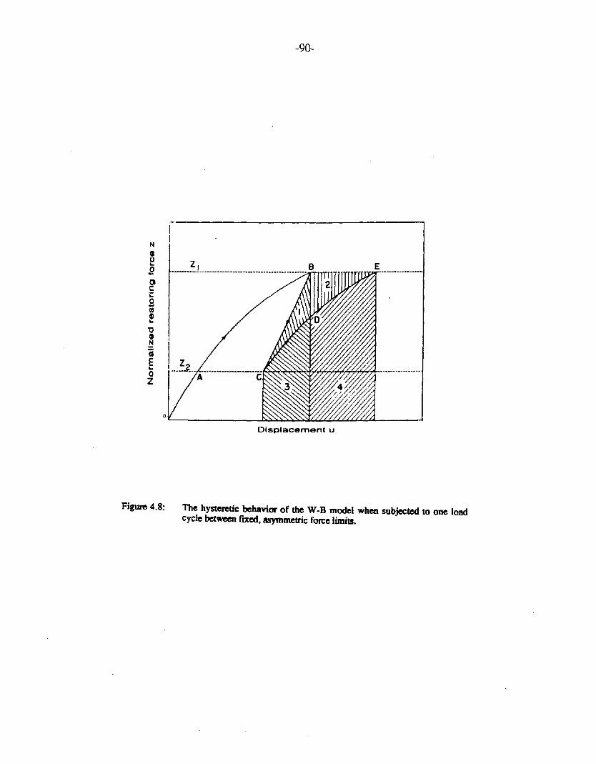
NGleSQc:.~
9Gl
!'0GlN
iE..oZ
-90-
.------------------,III
.~...,...."rr,..~Jii_········-····-·-
.~-_ _ __..
Displacement u
Figure 4.8: The hysteretic behavior of the W-B model when subjected to one loadcycle between fIXed, asymmetric force limits.
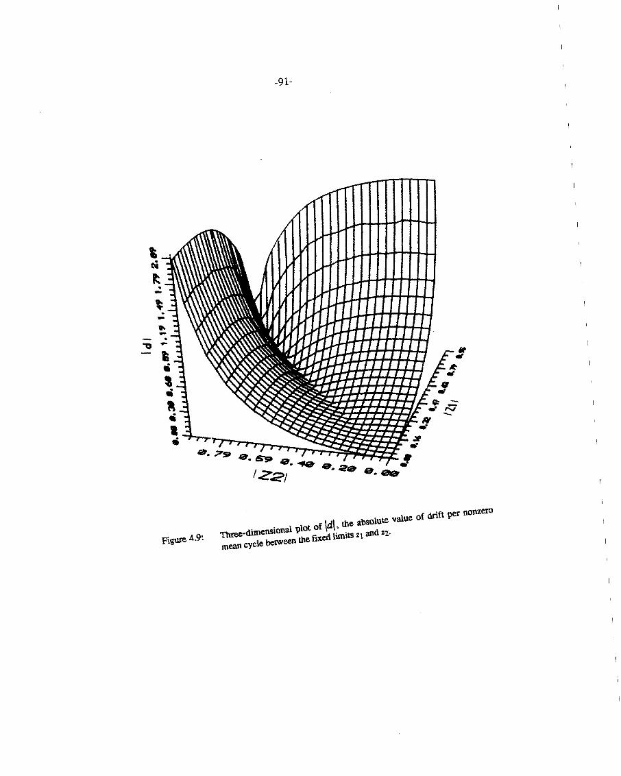
-91-
•-......-..•"'Q -
I)..,..~..,•
Pigure 4.9: nuee-diJneDSionai plot of \til. the abSOlu", value of drift per nooz<romean cycle betWeen the fixed limits %1 and %2·
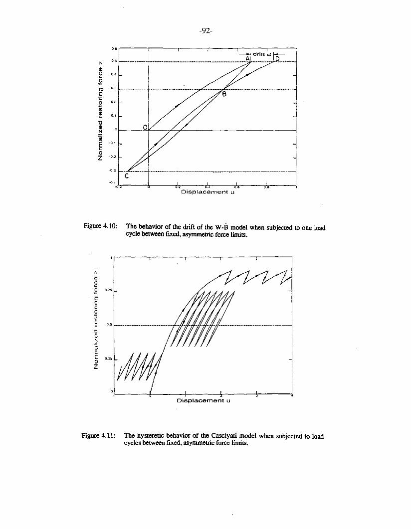
0.6
N0.5
Ql(J 0.4...0....Cl 0.3
c:'C0 0.2...(/)
Ql 0.1...'0Ql 0N
tilE -0.1
...0Z -0.2
-0.3
-0.4-0.
-92-
I ~driftd to......._- _ - --_ _- ..- _---- -----_ __ --- ---_........ - - ---
II-------------;....------_.._.-.._--_._-_.I
Io
Displacement u
Figure 4.10: The behavior of the drift of the W-B model when subjected to one loadcycle between fIXed, asymmetric force limits.
N
Ql(J...0 0.75....Clc:'C0...(/)
Ql...'0Q)N
tilE..0Z
Displacement u
Figure 4.11: The hysteretic behavior of the Casciyati model when subjected to loadcycles between fIxed, asymmetric force limits.
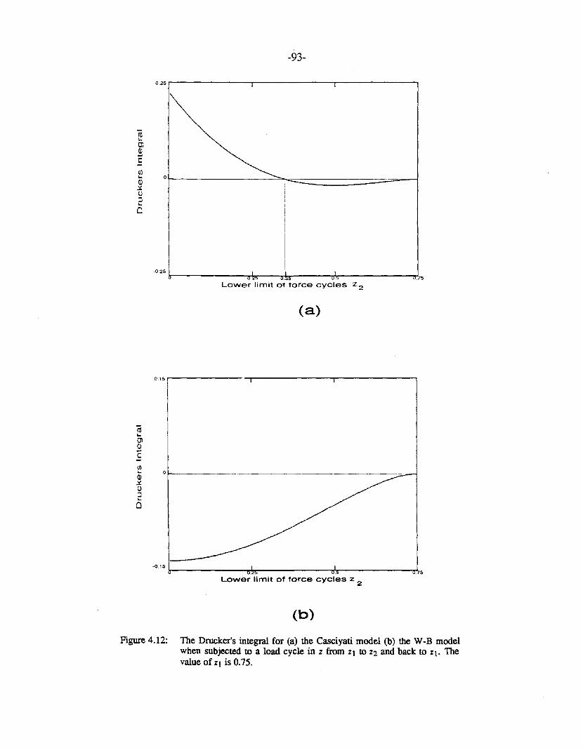
-93-
0.25r---------,--------r----------,
(ij'-ClQ)...C
Ul
~ °l---------==='";-O:::::::::::::============-I~(.J::l'-o
.0.251r--------,..;-\~-~I",-----.....,.L.:------____zrl,
Lower limit ot torce cycles z2
(a)
0.15r------- -r--------,----------,
(ij'-ClQ)...cUl~ 0t-------------------~(.J::l'-o
-0.15 ),-------..,...l,..-------*------~. 5Lower limit of force cycles z 2
(b)
Figure 4.12: The Drucker's integral for (a) the Casciyati model (b) the W-B modelwhen sUbjected to a load cycle in %from %1 to %2 and back to %1. Thevalue of %1 is 0.75.
-94-
CHAPTER 5
COMPARATIVE STUDY OF THE DYNAMIC PERFORMANCE
OF TWO HYSTERETIC MODELS
5.1 Introduction:
In Chapter 4, a set of quasi-static tests was performed on two classes of curvilinear
hysteretic models, namely, the Distributed Element type and the endochronic type. The
results presented indicated the difference in the behavior of the hysteretic restoring force
diagrams for the two classes of models in such features as loop closure, force relaxation,
energy dissipation and drift. In addition, it was shown that the endochronic models may
sometimes violate the Drucker's and Ilyushin's postulates. Such decidedly nonphysical
behavior exhibited by these models has also been pointed out previously [24,36,44].
However, these models have been used extensively for various applications in dynamics, a
few of which were listed in Chapter 4, with the most significant application being in the
response analysis of hysteretic systems by the method of equivalent linearization [10,54].
So far, no systematic investigation has been undertaken to determine how
appropriately the endochronic models represent real physical systems when subjected to
dynamic excitations such as earthquakes. Most comparisons so far, including those in
Chapter 4, have been carried out in a quasi-static manner and not dynamically where
inertial, viscous and other effects are present. This chapter compares the two model
responses when they are subjected to a variety of dynamic excitations, including
deterministic functions, recorded earthquake time histories, stochastic excitation, and
simulated earthquakes. The differences in some of the characteristic response quantities
serve as a measure of how satisfactory the endochronic model representation is for physical
systems.
-95-
In carrying out these analyses, the two models are adjusted to have identical initial
loading curves so as to facilitate direct comparison. For the Distributed Element model, the
extended Massing's hypothesis formulation is used because of the relative ease of
numerical implementation.
5.2 Hysteretic model representations:
Let !(u,u,Z) be the total restoring force in a system (Fig. 5.1) because of u, the
instantaneous relative displacement at instant t, U , the instantaneous relative velocity at
instant t, and Z, a vector that accounts for the dependence of! on the history of U up to
the instant t.
For a linear system,
!(U,U,Z) = cu + ku (5.1)
where c is the viscous damping coefficient, and k is the stiffness of the system. Since the
restoring force is dependent only on instantaneous quantities in the case of a linear system,
Z is the null vector.
In the case of the Wen-Bouc differential equation model,
!(u,u,Z) = aku +(1- a)kz + cu (5.2)
where k is the initial stiffness of the system, c is the viscous damping coefficient and a is
the ratio of the po~t-yielding stiffness to the initial stiffness. The only quantity accounting
for history dependence is the instantaneous value of z, which itself satisfies
i = Au - f3lulz + 'iUlzlThus, Z ={z}. Eqn. (5.3) is obtained by setting n=1, v =T1 =1.0 in Eqn. (2.38).
(5.3)
The initial loading behavior in the positive direction (Le., U > 0) is given by the
equation
(-ulu )z=z 1-e 'y (5.4)
-96-
where
Az ----
y - (/3 - r) . '1
u =---Y (/3 - r)
(5.5)
For ({3 - r) > 0, the initial loading behavior as shown in Fig. 5.2 has a limiting value of Zy
and an initial slope of A, Le., dZ/ = A.du ..=o
The ductility factor of the response, Jl , may be defmed with respect to uy as
uJl =.....!!!.
uy
(5.6)
where u". is the maximum absolute value of u, the response displacement to an excitation.
To be capable of withstanding an excitation without failing, a structure must be designed to
meet the ductility demand of the response that is due to the excitation. Generally speaking,
the larger the value of Jl that a structure can withstand without failing, the more ductile it
is. This factor plays a dominant role in the seismic design of a structure.
Popov [39] has reviewed experimental hysteresis loops for different structural
members and subassemblages constructed from different materials like steel, reinforced
concrete, etc. Maximum ductility demands of about 6.0 could be met by a steel cantilever
beam with welded connections as well as by an eccentrically braced steel frame. A
reinforced concrete cantilever beam and a framed reinforced concrete wall could meet
maximum ductiiity demands of about 4.0 and 3.5, respectively. A ductility ratio of 4.0 is
often used in design and analysis of structures, and this value has been adopted for several
examples in this chapter.
For the Distributed Element model in its extended Massing's hypothesis formulation
(Differential form),! satisfies Eqn. (5.2); Le.,
!(u,it, Z) =aku +(1- a)kz +cit
where a, k and c have the same meaning as in Eqn. (5.2), and
(5.2)
(5.7.1)
-97-
. . [ (,)(U-UN)]z = UIj/ sgn U 2
U = {U1,UZ, ,UN}T is an array. of N nested turning points, which is updated
continuously depending on the history of u in a manner set forth in Chapter 2. Ij/ is
defined as-WilL.
Ij/(u) == Ae', U E (0,00)
In this case, Z = {z,U1,UZ, ...... ,uNy.
(5.7.2)
It may be recalled that if U is the null vector, as in the case of virgin loading,
dz = lfI[u sgn(u)], u e (-00,00)du
(5.7.3)
It can be seen that for initial loading in the positive direction ( u> 0), the two hysteretic
models have the value of dz given by Ij/ as defined in Eqn. (5.7.2), leading to identicaldu
initial loading behavior.
In what follows, the Wen-Bouc differential equation model will be referred to as
the W-B model, and the corresponding Distributed ELement model with the same initial
loading curve as the DEL model.
5.3: Simple structural models:
5.3.1: Single-Degree-of-Freedom (SDOF) system:
Consider the simple structural model as shown in Fig. 5.3. This model consists of a
concentrated mass m in a gravitational field g at a height h above the ground. Assume that
the restoring force in the horizontal direction, f, can be described as in Sec. 5.2, and that
there is an external force F(t) acting on the mass. Assume also that there is a horizontal
excitation a(t) applied to the base of the structure. Let u and y be the horizontal and vertical
displacements of the mass, respectively. The equation of motion for u can be derived in the
following manner:
-98-
The Lagrangian of the system, L, can be written as:
L = .!.m[(u + ilg)2 +.ll - mg(h - y)2 .(5.8.1)
where ag is the displacement of the ground; that is, iig(t) = a(t). From the Lagrange's
equations,
!!.-(aL) _aL = net force in the horizontal direction,dt au au
= F(t) - f(u,u,Z) (5.8.2)
If e is the angle of rotation of the concentrated mass, the following relations can be-written
for u andy:
For small angles e,u =hSinO, y =h(l- CosO)
u =he and y =h0 2/ 2 => y =u2
/ 2h
(5.8.3)
(5.8.4)
Using this result in the Lagrange's equation yields the following equation of motion for u,
the horizontal displacement of the mass with respect to the ground:
with
mil + f(u,u,Z) - mg u = F(t) - ma(t)h
f(u,u,Z) = aku +(1- a)kz +eu
(5.9.1)
(5.9.2)
and z satisfies either Eqn. (5.3) or Eqn. (5.7), depending on the hysteretic model used.
The first-order effect of the gravitational field is to cause a reduction in stiffness.
There is thus a toppling effect, which may have a significant effect on the stability of the
system. More will be said about this in Sec. 5.5.2.
5.3.2 The MuIti-Degree-of-Freedom (MDOF) system:
A model for a multistory structure is shown in Fig. 5.4. Here the mass of the
structure is concentrated at only a few characteristic points along its height, usually at each
-99-
floor. Neglecting gravity, and assuming that there is a horizontal base excitation aCt), the
equations of motion for the interstory displacements ~,~, ,u" can be written as:
i
miCa +LUj ) + li(Ui,'Ui,Zi) - li+l(Ui+1,Ui+1,Zi+l) = 0 for i=l ,2,3, ..,(n-l) (5.10.1)j=l
"m,,(a+ LUj )+ 1"(u".u,,,Z,,) = 0
j=l
with each restoring force, Ii ' satisfying
Zi satisfies either Eqn. (5.3) or Eqn. (5.7), and mi is the mass of the itltstory.
The equations of motion can also be expressed as:
(5.10.2)
(5.10.3)
~+2.Il(~ z4,Zl) _2.12(~ ~,Z2) = -aCt) (5.11.1)~. m
1'
ui - -l-fi_l(Ui_l,Ui_l,Zi_l) +(_1_ +J...)fi(Ui,Ui,ZJ - J... fi+l(Ui+1,Ui+l,Zi+l) = 0mi- 1 mi_1 mi mi
where
for i=2,3, ....(n-l) (5.11.2)
(5.11.3)
(5.11.4)
5.4 Time integration procedure
The time integration of the equations of motion is accomplished by writing these
equations as a set of three first-order, ordinary differential equations (ODE) in the quantities
u, U and Z for each degree of freedom and then performing a fourth-order Runge-Kutta
integration with adaptive stepsize control. The technique employed is best explained in the
case of one independent variable, y, and one dependent variable, x.
-100-
Let the system be
: = f(x,y) (5.12)
where fis a known function of x and y. If y(x,,) = y", then the function y at X,,+l = x" + h is
estimated as follows:
"'. = hf(x",y,,)
Is = hf(x" + h ,y" + "'.)2 2
~ = hf(x,,+ ~ 'YII+ i)k4 = hf(x" + h,y" + k3)
Y,,+l = Y,. + .!. ("'. +2kz+2Js + k4 ) +O(h5)
6
(5.13.1)
(5.13.2)
(5.13.3)
(5.13.4)
(5.13.5)
In the case of a vector of unknown functions, a similar representation holds [17]. The
fourth-order Runge-Kutta is very commonly used in ODE integration.
Quite often, the step size h may be too large, and the truncation errors introduced may
be unacceptable. In dynamics, this may occur, for example, when finding the response of
an oscillator with a very short natural period compared to the integration time step h. A
good ODE integrator should exercise some adaptive control over its own progress, making
changes in step size, h, so as to keep the truncation error within bounds. The most
straightforward technique for the control of h is step-doubling. Each step is traversed
twice, once as a full step, and once as two consecutive half-steps. The following procedure
is then used to determine whether the step size should be reduced.
Lety(x+2h) be the exact solution for an advance from x to (x+2h), )l. the approximate
solution from Eqn. (5.13) for one step of size 2h, and yz the approximate solution from
Eqn. (5.13) for 2 steps of size h. Then,
-101-
y(x +2h) = Y1 +(2hi t/> +O(h6)
y(X +2h) =)2 +2hs t/> +O(h6)
(5.14.1)
(5.14.2)
The difference of the two numerical estimates, A, is a convenient indicator of the
truncation error
(5.15)
(5.16)
This error, A, must be kept less than some specified tolerance by adjusting h. Since Ais
proportional to hS and a step 2h results in an error A, the required step size 2 ho for an
acceptable error Ao can be estimated by
2~ = 2hl ~or·2
For Ao<A, Eqn. (5.16) provides an estimate of how much to decrease the step size when
the present step is repeated. For Ao>A, there is no need to decrease the present step size
2h.
For a system of first-order ODEs, the quantity Ao is actually a vector of desired
accuracies, one for each dependent variable. Eqn. (5.16) is used to get an estimate for 2~
for each dependent variable, and the step size is decreased according to the smallest of the
estimates.
5.5 Example 1: SDOF Structure with a suddenly applied external load:
5.5.1 Gravitational effects neglected:
Consider an SDOF oscillator of the type described in Sec. 5.3.1 with a kim ratio
corresponding to a nominal natural frequency of 1 Hz, no viscous damping and a value of
aof 0.05. The parameters of the nonlinear system, A, f3, r are taken to be 1.0, 0.12
em-I, and -0.08 cm-1, respectively. The ratio of f3lr =-1.5 is a typical value for the W-B
model, the parameter A=1.0 means dzldu =1.0 at u=O , and f3 is chosen such that uSC' the
-102-
nominal static displacement of the oscillator because of its self-weight mg, corresponds to a
ductility ratio of 5.0. That is, ust = 5.0, where uy = f3 1 and ust = mg .uy ( - r) k
In the absence of a base excitation and neglecting gravitational effects, the equation of
motion becomes
.. 1 f( . Z) F(t)U+- U,U, =--
m m(5.17)
where !(u,it,Z) has the usual meaning. The objective is to compare the response of the
two hysteretic models to a suddenly applied load. Such a situation could arise, for example,
when a steady gust of wind starts acting on a structure, or because of a sudden current on
ocean structures.
The increase in static pressure p that is due to a steady gust of wind may be expressed
as [1,43]:
(5.18.1)
where p is the mass density of air, V is the wind velocity, Ce is the exposure factor
depending on the height of the building, Cg is the gust factor, and Cp is the shape factor for
the building as a whole. Assuming p=1.26 kg/m3, Ce =1.5, Cg=2.0, Cp =1.3, it can be
shown that an 80 kmph wind causes an equivalent pressure of about 1250 N/m2. That is,
p = 1250(~JN/m2 (5.18.2)
where V is the wind speed in kmph. Assuming a 10 story structure with a plan area of 20
m by 20 m, a height of 35 m, a mass density for the structure of 1000 kg/m2/story, and a
wind velocity of 80 kmph, the wind force per unit mass F(t)/m is found to be equal to be
about 0.02 g. This wind force might be assumed to be a step function in time acting on the
structure that is initially quiescent.
-103-
The two models respond quite differently when subjected to the step forcing function.
Fig. 5.5 compares the displacements of the two models relative to the ground. The drifting
characteristic in the displacement of the W-B model is clearly evident. After 140 seconds,
the displacement for the W-B model is about 6 times that of the DEL model.
In Fig. 5.6, a comparison is made of the hysteretic restoring force diagrams. The
same drifting is again quite evident in the response of the W-B model. By comparison, the
DEL model settles down to a stable closed loop. The distinguishing feature noticeable in
Fig. 5.6 is that there is a gradual hysteretic force relaxation in the W-B model. As a matter
of fact, if the motion is observed for a long enough time, the mean hysteretic restoring
force in the W-B model will settle down to a zero value. If ii and z are the steady-state
mean values of u and z, then on neglecting inertial effects, the equation of motion yields
akii +(1- a)kz = 0.02mg (5.19)
Since z=O for the W-B model, ii=0.50633/ a. For a=0.05, Eqn. (5.19) is satisfied in
the case ofthe W-B model by z=O, ii=1O.127 cm. By comparison, in the case of the DEL
model, the equation is satisfied in steady state by z=O.503 em and u=O.570 em as seen in
Fig. 5.6.
Fig. 5.7 compares the relative velocity response of the two models for a =0.05.
The agreement is very good. For the first 25 seconds, the behavior is almost identical. For
the next 50 seconds, a slight elongation in the period of the system is observed for the W-B
model, but is otherwise satisfactory.
Fig. 5.8 shows the displacement response of the W-B model for different values of
a, namely, 0.0, 0.05, 0.25 and 0.50. The corresponding steady-state values, ii, are 00,
10.127,2.025 and 1.013 cm., respectively.
In summary, for suddenly applied loads, it can be said that there is good agreement in
response quantities like relative velocity (Fig. 5.7) and maximum hysteretic force (Fig.
5.6), but there can be large discrepancies in relative displacement and ductility. Whether the
-104-
use of the Wen-Bouc model is appropriate therefore depends on what response quantity is
being elicited from the model.
5.5.2 Gravitational effects included:
In the presence of a gravitational field, a structure of the type descrIbed by Sec.
5.3.1 has a term -mgu/h on the left-hand side of the equation of motion (Eqn. 5.9). This
results in a reduced system stiffness that introduces a negative restoring force tending to
topple the structure, a phenomenon often described as the P - 8 effect. This tendency to
collapse is not due to the deterioration of the mechanical properties of the members, but
rather is due to the large geometrical changes that take place. For large displacements, the
experimental hysteresis loops for subassemblages in [39] display negative slopes
associated with the motion of the subassemblage as a mechanism aided by the P - 8
effect.
In the absence of a base excitation, the equation of motion can be written as:
.. 1 I( . C't) k F(t)u+- U,u,~ -11-u=--m m m
(5.20)
where I has the usual meaning, and where 11~ = g. As in Sec. 5.5.1, let the nominalm h
natural frequency=1.0 Hz, A=1.0, /3=0.12 em-I, r=-0.08 em-I, F(t)/m=0.02 g, h=35
m. Thus, 11 =0.071. There is assumed to be no viscous damping.
For a> 11, no change is expected from the results in Sec. 5.5.1, since the post
yielding stiffness is reduced but is still greater than O. However, for a < 11, the post-
yielding stiffness has a negative value. Given the manner in which the displacement drift of
the W-B model increased when the post-yielding stiffness was decreased in Sec. 5.5.1
(Fig. 5.8), the drift for the system with negative post-yielding stiffness may be expected to
be even larger. Figs. 5.9 and 5.10 compare the displacements and restoring force diagrams
respectively, for the case a =0.05. After 140 seconds, the displacement of the W-B model
-105-
is about 8 times that of the DEL model. As a matter of fact, u for the W-B model will keep
increasing as the time of observation increases. The other difference observed is that the W
B model does not exhibit the hysteretic force relaxation in Fig. 5.10 as was noted in Fig.
5.6. Actually, to counter the decrease in the restoring force that is due to the P - 8 effect, Z
and therefore the hysteretic force increase. This will go on until the increase of z will no
longer be enough to offset the destabilizing force, T] ku, and the W-B model will predict
catastrophic failure, even though from the DEL model, it is seen that a constant force of
0.02 g per unit mass of the structure does not, in fact, lead to the failure of the structure.
These features are more evident for larger values of T]. For example, Figs. 5.11 and
5.12 compare the relative displacement history and restoring force diagram for T] =0.25. It
can be seen that the W-B model predicts collapse at about 90 seconds after the load is fIrst
applied. This is not the case with the DEL model, which has a steady-state mean offset of
about 1 em. From a physical viewpoint, it seems highly unlikely that a 80 kmph wind
would lead to the collapse of the structure. Hence, the failure predicted by the W-B model
can be attributed to the instability of the mathematical representation of the model rather
than to the inability of the structure to withstand the load.
It is concluded that extreme caution must be exercised when the Wen-Bouc model is
used to study the response of structures exhibiting unstable behavior. If the Wen-Bouc
model is used to describe the hysteretic nature of a system and the ensuing analysis predicts
failure, it might not be possible to tell whether the result is spurious, arising from the
inherent instability of the mathematical representation of the model, or whether the structure
actually failed because of excessive loading. It may be prudent not to employ the Wen
Bouc model representation for any nonlinear hysteretic system with a negative post
yielding stiffness.
-106-
5.6 Example 2: Structure sUbjected to earthquake excitation:
5.6.1 SDOF system:
Consider an SDOF oscillator of the type described in Sec. 5.3.1 with a kim ratio
corresponding to a nominal natural frequency of 1.0 Hz, c such that the viscous damping
coefficient is 5% of critical, and a value of a of 0.05. The parameters describing the
nonlinear behavior, A, /3 and r are 1.0, 25.25 m- l and -18.15 m- 1 (i.e·'/3lr =-1.5),
respectively. The value of /3 is such that the maximum displacement of the oscillator with
the hysteresis described by the DEL model corresponds to a ductility value of 4.0 when
subjected to the NS component of 19~0 EI Centro earthquake (Fig. 5.13). For the selected
values of A, /3 and r, uy=zy=0.022 m. There is no external force F(t), gravitational
effects are neglected and the structure is assumed to be initially quiescent. The response of
the two models is numerically computed for a duration ofT=50 seconds.
Figs. 5.14-5.17 show the hysteretic restoring force diagrams, U vs. t, Z vs. t and uvs. t, respectively. The following observations may be noted:
(1) The restoring force diagrams are qualitatively and quantitatively different as seen from
Fig. 5.14. Firstly, nonclosure of some loops is quite evident in the W-B model.
Secondly, it is observed that the unloading branches are stiffer for the W-B model than
for the DEL model. The consequence of the first difference is that there may be portions
of the response where negative energy is dissipated by the W-B model, while that of
the second difference is that the loops in the W-B model enclose larger areas and hence
result in a larger dissipation of energy.
(2) The basic nature of the displacement response time histories for the W-B and DEL
models is quite similar (Fig. 5.15). There is close agreement in the absolute value of the
maximum displacement (0.087 and 0.088 m, respectively), and in the dynamic
amplitude, which is the difference between the largest and smallest values of the
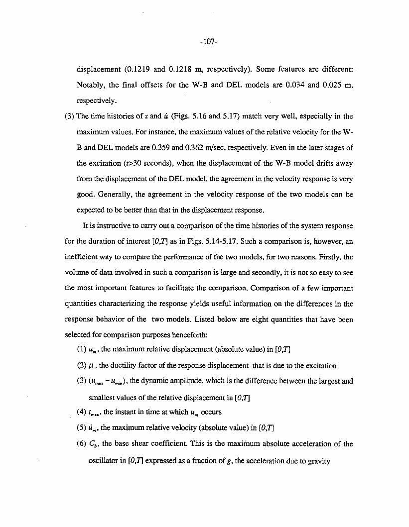
-107-
displacement (0.1219 and 0.1218 m, respectively). Some features are different:·
Notably, the final offsets for the W-B and DEL models are 0.034 and 0.025 m,
respectively.
(3) The time histories of z and U (Figs. 5.16 and 5.17) match very well, especially in the
maximum values. For instance, the maximum values of the relative velocity for the W
B and DEL models are 0.359 and 0.362 rn!sec, respectively. Even in the later stages of
the excitation (t>30 seconds), when the displacement of the W-B model drifts away
from the displacement of the DEL model, the agreement in the velocity response is very
good. Generally, the agreement in the velocity response of the two models can be
expected to be better than that in the displacement response.
It is instructive to carry out a comparison of the time histories of the system response
for the duration of interest [O,T] as in Figs. 5.14-5.17. Such a comparison is, however, an
inefficient way to compare the performance of the two models, for two reasons. Firstly, the
volume of data involved in such a comparison is large and secondly, it is not so easy to see
the most important features to facilitate the comparison. Comparison of a few important
quantities characterizing the response yields useful information on the differences in the
response behavior of the two models. Listed below are eight quantities that have been
selected for comparison purposes henceforth:
(1) u"" the maximum relative displacement (absolute value) in [O,T]
(2) J.l , the ductility factor of the response displacement that is due to the excitation
(3) (umax - umin ), the dynamic amplitude, which is the difference between the largest and
smallest values of the relative displacement in [O,T]
(4) tmax , the instant in time at which u'" occurs
(5) U"', the maximum relative velocity (absolute value) in [O,T]
(6) Cb , the base shear coefficient. This is the maximum absolute acceleration of the
oscillator in [O,T] expressed as a fraction ofg, the acceleration due to gravity
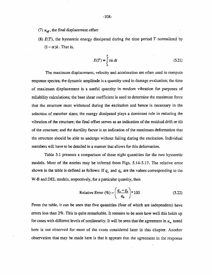
-108-
(7) Uoff ' the fmal displacement offset
(8) E(n, the hysteretic energy dissipated during the time period T normalized by
(1- a)k. That is,
T
E(T) = Jzudto
(5.21)
The maximum displacement, velocity and acceleration are often used to compute
response spectra; the dynamic amplitude is a quantity used in damage evaluation; the time
of maximum displacement is a useful quantity in random vibration for purposes of
reliability calculations; the base shear coefficient is used to detennine the maximum force
that the structure must withstand during the excitation and hence is necessary in the
selection of member sizes; the energy dissipated plays a dominant role in reducing the
vibration of the structure; the fmal offset serves as an indication of the residual drift or tilt
of the structure; and the ductility factor is an indication of the maximum deformation that
the structure should be able to undergo without failing during the excitation. Individual
members will have to be detailed in a manner that allows for this deformation.
Table 5.1 presents a comparison of these eight quantities for the two hysteretic
models. Most of the entries may be inferred from Figs. 5.14-5.17. The relative error
shown in the table is defined as follows: If qa and qb are the values corresponding to the
W-B and DEL models, respectively, for a particular quantity, then
Relative ElTOr (%) = ( q.;.q,)* 100 (5.22)
From the table, it can be seen that five quantities (four of which are independent) have
errors less than 2%. This is quite remarkable. It remains to be seen how well this holds up
for cases with different levels of nonlinearity. It will be seen that the agreement in u'" noted
here is not observed for most of the cases considered later in this chapter. Another
observation that may be made here is that it appears that the agreement in the response
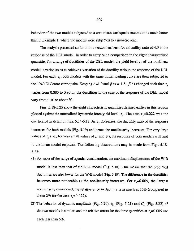
-109-
behavior of the two models subjected to a zero mean earthquake excitation is much better
than in Example 1, where the models were subjected to a nonzero load.
The analysis presented so far in this section has been for a ductility ratio of 4.0 in the
response of the DEL model. In order to carry out a comparison in the eight characteristic
quantities for a range of ductilities of the DEL model, the yield level Zy of the nonlinear
model is varied so as to achieve a variation of the ductility ratio in the response of the DEL
model. For each Zy, both models with the same initial loading curve are then subjected to
the 1940 El Centro earthquake. Keeping A=l.O and f3 /r =-1.5, f3 is changed such that Zy
varies from 0.005 to 0.90 m; the ductilities in the case of the response of the DEL model
vary from 0.10 to about 30.
Figs. 5.18-5.25 show the eight characteristic quantities defined earlier in this section
plotted against the normalized hysteretic force yield level, Zy. The case zy=0.022 was the
one treated in detail in Figs. 5.14-5.17. As Zy decreases, the ductility ratio of the response
increases for both models (Fig. 5.19) and hence the nonlinearity increases. For very large
values of Zy (i.e., for very small values of f3 and r), the response of both models will tend
to the linear model response. The following observations may be made from Figs. 5.18
5.25:
(1) For most of the range of zyunder consideration, the maximum displacement of the W-B
model is less than that of the DEL model (Fig. 5.18). This means that the predicted
ductilities are also lower for the W-B model (Fig. 5.19). The difference in the ductilities
becomes more noticeable as the nonlinearity increases. For Zy=0.005, the largest
nonlinearity considered, the relative error in ductility is as much as 15% (compared to
about 2% for the case zy=0.022).
(2) The behavior of dynamic amplitude (Fig. 5.20), U", (Fig. 5.21) and Cb (Fig. 5.22) of
the two models is similar, and the relative errors for the three quantities at Zy=0.005 are
each less than 6%.
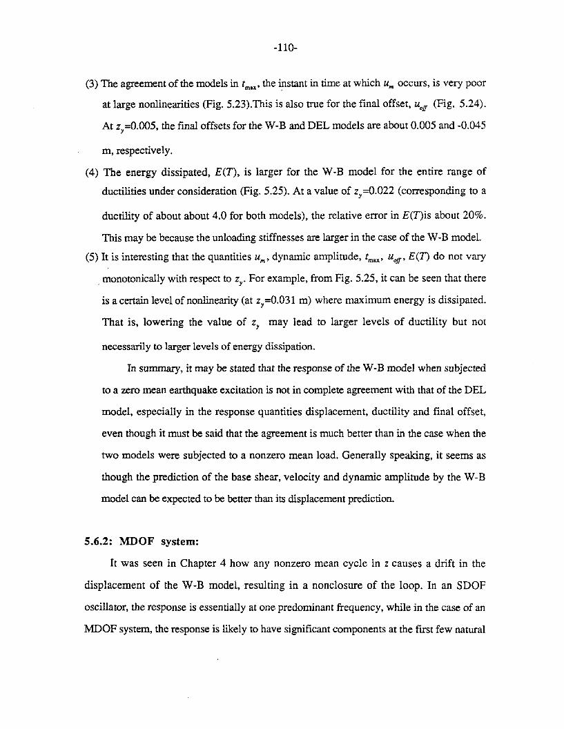
-110-
(3) The agreement of the models in tmax , the instant in time at which u". occurs, is very poor
at large nonlinearities (Fig. 5.23).This is also true for the final offset, uoff (Fig. 5.24).
At z =0.005, the final offsets for the W-B and DEL models are about 0.005 and -0.045y
m, respectively.
(4) The energy dissipated, E(T), is larger for the W-B model for the entire range of
ductilities under consideration (Fig. 5.25). At a value of zy =O.022 (corresponding to a
ductility of about about 4.0 for both models), the relative error in E(T)is about 20%.
This may be because the unloading stiffnesses are larger in the case of the W-B model.
(5) It is interesting that the quantities u"., dynamic amplitude, tmax ' uoff ' E(T) do not vary
. monotonically with respect to Zy. For example, from Fig. 5.25, it can be seen that there
is a certain level of nonlinearity (at Zy=0.031 m) where maximum energy is dissipated.
That is, lowering the value of Zy may lead to larger levels of ductility but not
necessarily to larger levels of energy dissipation.
In summary, it may be stated that the response of the W-B model when subjected
to a zero mean earthquake excitation is not in complete agreement with that of the DEL
model, especially in the response quantities displacement, ductility and final offset,
even though it must be said that the agreement is much better than in the case when the
two models were subjected to a nonzero mean load. Generally speaking, it seems as
though the prediction of the base shear, velocity and dynamic amplitude by the W-B
model can be expected to be better than its displacement prediction.
5.6.2: MDOF system:
It was seen in Chapter 4 how any nonzero mean cycle in Z causes a drift in the
displacement of the W-B model,resulting in a nonclosure of the loop. In an SDOF
oscillator, the response is essentially at one predominant frequency, while in the case of an
MDOF system, the response is likely to have significant components at the first few natural
-111-
frequencies of the system. A similar situation may also arise in the case of an SDOF
oscillator when the excitation is predominantly at a frequency different from that of the
natural frequency of the oscillator, resulting in a response with two peaks in its frequency
spectrum. In either case, the tendency of the W-B model to drift, have nonclosure of loops,
etc., may be more pronounced because the response will have high-frequency components
superposed over a low-frequency component, and these high-frequency components cause
additional cycles in z over a nonzero mean. A hysteretic restoring force is frequency
independent; thus, a nonzero mean cycle in z will result in the same amount of drift
irrespective of the frequency associated with that cycle. Therefore, in an MDOF system, the
drift in the displacement of the W-B model is likely to be larger than in an SDOF system.
To demonstrate this qualitatively, the two-story structure shown in Fig. 5.26 is
considered. The initial stiffness-to-mass ratios are such that the nominal natural frequencies
of the system are 0.5 and 1.5 Hz. There is assumed to be no viscous damping, and the
post-yielding stiffness ratio a equals O. The nonlinear parameters describing the nonlinear
behavior are: ~=Az=l.O, f3 2 /r2=f3Jrl=-1.5, f32=f31=18.00 m- 1.The f3s are
chosen such that the maximum displacement of the fIrst story of the DEL model to the EI
Centro earthquake corresponds to a ductility of about 4. For the purposes of this
comparison, gravity effects are neglected, and there are no external forces acting on the
structure.
Figs. 5.27 and 5.28 compare the interstory displacements of the ftrst and second
stories, respectively. The maximum displacement in the fIrst story is 0.130 m (a ductility
ratio of 3.90) in the case of the DEL model and is 0.180 m (a ductility ratio of 5.40) in the
case of the W-B model.
It is also interesting to compare the fIrst story's restoring force diagrams of the two
models (Fig. 5.29). In Fig. 5.29a, two segments in the restoring force diagram of the W-B
model associated with drift and nonclosure of loops are shown in dashed lines. These
-112-
occur at about 3 seconds and 12 seconds after the earthquake commences. By observing
the displacement of the fIrst story (Fig. 5.27) at these instants in time, it can be seen that the
segments are due to the high-frequency component of the response. In addition, the usual
contribution to drift due to the nonzero mean cycling corresponding to the low frequency
component is also present, as in the case of the SDOF system.
It may be noted that the discussions in this section are for one specific base excitation.
While useful information can be gathered about the nature of the responses of the two
hysteretic models to earthquake excitations from the example considered, for more
quantitative comparisons, a stochastic analysis will be performed in the next section with
ensembles belonging to different families of excitations..
5.7 Stochastic excitation:
5.7.1 Introduction:
If the state of stress, the material properties, location and history of fractures and
other requisite details are known, and the tectonic mechanisms causing earthquakes are
completely understood, the ground motion aCt) at a given site can be theoretically computed
in advance. Since all the required information is rarely available, engineers and scientists
must accept a certain level of uncertainty or randomness in describing the earthquake
ground motion. For this reason, earthquake motion is often represented by a stochastic
process. Use of a stochastic model to describe earthquake motion is appropriate in much
the same way as the use of probabilistic models in the characterizations of errors in
measurements of physical quantities such as structural stiffnesses.
One suitable approach in the selection of stochastic models to describe earthquake
motion is in defining the excitation as.belonging to a general class of time histories. The
class of time histories should have time- and frequency-domain properties that will
realistically reflect the features of an actual earthquake, like the frequency content, duration
-113-
of shaking, peak acceleration, etc. The larger the number of features the earthquake model
has to include, the larger will be the number of parameters to describe the model. The only
limitation in the selection of the complexity of the stochastic models is that the analytical
methods for the analysis of nonlinear systems subjected to random excitation are much
more complex than in the case of a simple deterministic input. Therefore, the stochastic
model description for earthquake motion must be as simple as possible. Also, from the
point of view of numerical simulation analysis such as carried out here, the stochastic
models need to be simple enough so that only a small computational effort is spent in
generating the ensemble of excitation time histories.
In this section, two classes of stochastic excitation are chosen for. which a
comparative response study is performed of the eight characteristic quantities defined in
Sec. 5.6. The two types of random processes are stationary white noise and response
spectrum-consistent time histories. The following two sections explain the manner in which
the ensembles are generated and compare the response of the two hysteretic models to the
ensembles.
5.7.2 Example 3: SDOF system with stationary white noise base excitation:
One of the simplest random processes is a zero mean, Gaussian stationary process.
Because stationary processes are well understood and the theory is well developed, much
effort has been devoted in earthquake engineering research to model earthquakes as
stationary processes. One such approach has been to use stationary white noise; Housner
[18] suggested a model that was essentially white noise - a large number of impulses
arriving at random times. The white noise model has been used extensively to investigate
structural behavior during earthquakes [9,42]. Clearly, stationary excitations can be used
only to represent the strong shaking portion of an earthquake record, not for the buildup or
-114-
tail of the ground motion. The simplicity of the white noise random process has ensured its
continued use in current research as a stochastic model to describe earthquake motion.
Let the base excitation n(t) be a zero mean, stationary, Gaussian white noise with a
spectral density So' Let there also be a constant external force per unit mass F on the
structure and let gravitational effects be neglected. For the purpose of carrying out a Monte
Carlo simulation with white noise, an ensemble of Fi sample functions is generated for
n(t). Each sample function is constructed in the following manner: A sequence of
independent Gaussian distributed numbers with a zero mean and unit variance is generated.
The numbers are used as ordinates of the function at equally spaced intervals in time, !it.
The function is then assumed to vary linearly within each time interval. On multiplying the
function by (21CSoI !it)1/2, it can be shown [15] that the power spectral density of the
function approaches So as the m!it approaches zero and remains within 5% of So for
co!it<O.57, m being the frequency. Therefore, to approximate a white noise process to
within a given tolerance up to a desired frequency, the time interval chosen must be
appropriately small. In this example, !it=O.02 seconds.
Most digital computers have only a library subroutine that generates pseudo-random
numbers uniformly distributed on [0,1]. From two such numbers Xl and x2 ' two
independent numbers, Zl and Z2' belonging to a Gaussian distribution with zero mean and
unit variance can be generated using the following relations [15]:
(5.23)
In this manner, Fi samples of zero mean, stationary, Gaussian white noise, each
lasting 20 seconds, are generated, this time period being a typical earthquake duration. A
simulation analysis is performed for each of the six cases listed in Table 5.2. For each case,
a comparison is made between the two models of the eight characteristic response quantities
described in Sec. 5.6. For all six cases, the following are kept constant: nominal natural
-115-
frequency of 1 Hz, viscous damping as a fraction of critical 5%, the ratio f3 /r of
-1.5 and A=1.0. The parameters that are varied in the six cases of Table 5.2 are a, F, and
f3 . In Cases I, II and III, there is no post-yielding stiffness, there is no external force
(F =0), and f3 is changed so as to vary the level of nonlinearity; for the three values of f3
considered, the mean values of the predicted ductilities in the response of the DEL model
are about 2.0, 4.0 and 8.0. Thus, the manner in which the response statistics of the two
hysteretic models vary over a range of ductilities may be observed. The motivation behind
the choices of the remaining cases listed in Table 5.2, namely, Cases IV, V and VI is to
study the effect of positive post-yielding stiffness, nonzero mean loading, and combined
positive post-yielding stiffness and nonzero mean loading, respectively.
To examine the convergence rate of the mean and standard deviation of u'" in Case
ill, statistics are obtained for a variation of the number of samples, Fi, from 5 to 1000. For
both models, the means converge faster than the standard deviations, as should be
expected. After 250 simulations, the standard deviations for the W-B and DEL models are
within 3% and 8% of their respective values after 1000. For the remainder of this section,
Fi =250 samples are considered large enough for the calculation of the response statistics.
For each case listed in Table 5.2, the two systems with hysteresis described by the
W-B and DEL models and initially at rest with zero velocity are subjected to the ensemble
of ground acceleration and external force F, and the responses are computed for a time
duration of T=30 seconds. From the respective responses, statistics of the eight
characteristic response quantities under consideration are calculated and tabulated in detail
in Tables 5.3 through 5.8, respectively, for the six cases. The statistics displayed for each
quantity are the mean, the standard deviation and the median. For a symmetric distribution,
the mean and the median are the same. Also recorded in the tables are the statistics of the
relative error for all eight quantities except uoff ' This is because the final offset for zero
-116-
mean loading has a zero mean, and the values of uoff close to zero will cause a large relative
error in Eqn. (5.22), leading to misleading figures.
Values from Tables 5.3, 5.4 and 5.5 are used to plot Figs. 5.30-5.35, which show
u"., f.l, Li"., Cb , uoff and E(n, respectively, vs. the yield level of the normalized hysteretic
force,Le., Zy. The three values of Zy corresponding to Cases I, II and III, are 7.82, 5.00
and 3.42 ems, respectively. The smaller the value of Zy, the larger is the ductility (Fig.
5.31) and hence larger the nonlinearity. In Figs. 5.30-5.35, three curves are drawn for
each hysteretic model, corresponding to the values of (i) mean minus one standard
deviation, (ii) mean, and (iii) mean plus one standard deviation of the response quantity.
Thus, an idea can be obtained not only of the mean value comparison but also of the
standard deviation. The following observations may be made from Figs. 5.30-5.35 and
Tables 5.3, 5.4 and 5.5:
(1) From Figs. 5.30 and 5.31, it is seen that the values of u". and ductility are likely to be
larger for the W-B model. For both models, the standard deviation increases as the
nonlinearity increases. The mean and standard deviation in u". for the W-B model are
about 1.25 and 1.75 times that of the DEL model for Case II, and the mean relative
error is 27%. The use of the W-B model would therefore lead to a more conservative
design with structures designed for larger ductilities than would be necessary according
to the DEL model.
(2) The relative error in the dynamic amplitude for Case II has a mean value of about 7%,
meaning that on an average, the W-B model overestimates the dynamic amplitude value
of the DEL model by about that amount. In specific instances, however, the estimation
may be more or less since the error has a standard deviation of about 22%.
(3) The relative errors involved in the estimation of tmax by the W-B model are very large
(mean of 76% and standard deviation of 222% for Case II). This means that the use of
the W-B model in reliability calculations will lead to erroneous results.
-117-
(4) The maximum velocity (u", ) values for the W-B model are somewhat less than for the
DEL model (Fig. 5.32). For Case II, the mean and standard deviation of U'" are about
60 ems/sec and 7 ems/sec, respectively, for the W-B model and 65 ems/sec and 8
ems/sec respectively for the DEL model, and the mean relative error is about -7.5%.
Given this information, one may make the decision that U'" predictions by the W-B
model are quite acceptable, but this is a subjective matter requiring some consensus on
what is "acceptable" error.
(5) Among the eight quantities under discussion, the one in which by far the best agreement
is observed among the two hysteretic models is in Cb , the base shear coefficient (Fig.
5.33). The means of Cb for Case II are 0.214 and 0.216, respectively, for the W-B and
the DEL models, and the mean relative error is about -1%.
(6) The final offset is a quantity that should be expected to have a zero mean and from Fig.
5.34, this is seen to be essentially true for both models. However, the standard
deviations are much larger for the W-B model than for the DEL model, especially at
higher levels of nonlinearity. For Case II, the standard deviation of the W-B model is
more than 2.25 times that of the DEL model; Le., the final offset value is likely to be
larger for the W-B model, and that would imply that larger damage has occurred than
actually did according to the DEL model.
(7) The values of the energy dissipated, E(T), for the W-B model are consistently larger
than those for the DEL model (Fig. 5.35). This overestimation by the W-B model was
observed in Sec. 5.6, too. In Fig. 5.36, it appears that there is only a translational shift
in curves: for the three values of Zy considered, the means differ by a constant value,
while the standard deviations are essentially the same. For Case II, the mean value
estimate of E(T) by the W-B modelis 1.07 times that of the DEL model.
On the basis of these observations, a few remarks may be made here. For systems
with no post-yielding stiffness, the W-B model provides an excellent estimate of the value
-118-
of the base shear coefficient Cb , while estimates by the W-B model of the maximum
velocity it"" the dynamic amplitude and the energy dissipated E(T), appear to be adequate.
But the estimates by the W-B model of the maximum displacement, u'" (and hence of the
ductilities), the final offset, uolf ' and the time of maximum displacement, tmax , are much
less reliable. It is not immediately apparent if the trends noted here are unchanged for
systems with different nonlinear parameters (different f3 /r , A, etc.), but the analysis
performed here gives an idea of how the two models compare.
For complete in~ormation on the statistical nature of each response quantity, it would
be necessary to know the probability density function. For Case III, a comparison of the
probability density functions for a few quantities is carried out. Fig. 5.36 shows the
probability density function of u"" the maximum absolute value of the relative
displacement. The two models exhibit similar behavior in the probability density, but it can
be seen that the mean value and standard deviation for the W-B model (about 34 cms and
14.5 cms, respectively) are larger than for the DEL model (about 28 cms and 11 cms,
respectively). The density functions resemble Rayleigh distributions even though there is
not enough information on the behavior for values of u'" less than 15 cms.
If u'" for each hysteretic model is normalized by subtracting the respective mean and
dividing by the respective standard deviation and the probability density functions plotted
as in Fig. 5.37, it can be seen that they follow the same basic distribution. This would
seem to suggest that the differences in the means and standard deviations of the two models
are adequate to characterize the differences in their probability densities.
Fig. 5.38 shows the cumulative probability function (the integral of the probability
density function) of u"" The medians for the W-B and DEL models are about 31 cms and
25.5 cms, respectively. In random vibration, the reliability function W(I) is defined as the
probability that the magnitude of U does not exceed a specified level b throughout the time
interval [O,T] . Fig. 5.38 is therefore also the plot of W(30) for values of b on the
-119-
horizontal axis from 0 to 100 cms. Thus, the reliability function used in the fIrst passage
problem is different for the two hysteretic models, and the probability that um is less than
any specified value b (also called the "safe" probability) is larger for the DEL model than
for the W-B model.
Figs. 5.39 and 5.40 show the probability density functions for Case III of the
maximum relative velocity, um' and the base shear coeffIcient, Cb , respectively. These
probability densities are more symmetric than um ' and the predictions of Cb by the two
models match very closely. For um ' the mean relative error is about -7%; this accuracy may
or may not be enough depending on the allowable error tolerance.
Fig. 5.41 is the probability density function of uojf ' the final offset which is almost
zero mean for both hysteretic models, but the spread or standard deviation for the W-B
model is 1.5 times that of the DEL modeL The fInal offset of the W-B model is therefore
likely to be larger than that of the DEL modeL For example, it can be seen from Fig. 5.41
that the probability that uojf will between 49 and 51 cms is larger for the W-B modeL
Case IV is the same as Case II in every aspect except that a is 0.05 for Case IV
instead of 0 as in Case II; Le., the system has a post-yielding stiffness equal to 5% of the
initial stiffness and thus there is a positive linear restoring force. The effect of such a linear
spring is to control the displacement drift of the W-B model, and one should therefore
expect that um (and J1) values of the W-B model for this case should be closer to those of
the DEL model than in Case II. This indeed is true. From Tables 5.4 and 5.6, it is seen that
though there is some marginal improvement in most of the eight quantities, the most
dramatic is in um ' The mean and standard deviation of this quantity are about 18 ems and
4.5 ems, respectively, for both models. This would suggest that for systems with positive
post-yielding stiffnesses (a >0), the W-B model may be a more suitable description of
hysteresis than for systems without (a =0).
-120-
In Case V, an external static load (F -:# 0) is added to the zero mean white noise
ensemble in order to study the effect of nonzero mean loading. F is 2% g which, as was
seen in Sec. 5.5.1 would correspond approximately to a 80 kmph wind on a 10 story
structure. Cases II and V have the same parameters; the only difference is that Case V has a
nonzero F. Direct comparison of Tables 5.4 and 5.7 will thus show the effect of the static
load. From the example in Sec. 5.5.1, one should expect the u'" differences to be much
larger for Case V than for Case II. A look at Table 5.7 confmns this. For Case V, the mean
and standard deviation in u'" of the W-B model are almost 1.75 and 2.25 times that of the
DEL model (compared to the corresponding factors 1.25 and 1.75 for Case II). The
external static load has the effect of increasing the mean value of the ductility J.l from 3.94
to 4.42 for the DEL model and from 4.93 to 7.59 for the W-B model. The following
conclusion may therefore be drawn: The hysteretic representation given by the W-B model
provides unreliable estimates of the response statistics of systems with no post-yielding
stiffness subjected to a nonzero mean loading. The case of nonzero mean loading is not a
favorable one for the use of the W-B model as description of system hysteresis.
Case VI involves having a nonzero mean loading as well as a positive a (a=5%).
This enables the combined effect of having a nonzero mean loading condition (unfavorable
for the W-B model) and a positive post-yielding stiffness (favorable for the W-B model).
Considering Tables 5.4,5.7 and 5.8, it can be seen that the effect of a >0 not only reduces
the detrimental effect of the nonzero mean loading in the response of the W-B model, but
actually provides a better agreement in the response statistics than in Case II (but not as
good as in Case IV).
5.7.3 Example 4: Comparison of inelastic response spectra:
The response spectrum is a common means of specifying earthquake ground motion
for structural response studies. It is appealing because it gives some of the most important
-121-
features of the response without requiring knowledge of the time history of the excitation.
In spite of its advantages, the response spectrum has one glaring shortcoming as a design
specification. It is normally defined only in relationship to linear systems. This can be a
severe limitation because most modern building structures are designed to behave in a
nonlinear, ductile manner during a major earthquake. One way to overcome this difficulty
may be in the definition of an inelastic response spectrum associated with a given elastic
response spectrum. It is believed that for many buildings, satisfactory approximations to
the design forces and deformations can be obtained from the modal method by using the
corresponding inelastic response spectrum. Veletsos and Newmark [51] , Iwan [23] and
others have given methods for estimation of inelastic response spectra from their elastic
counterparts for simple piecewise-linear hysteretic models.
Because it is desired to determine the inelastic response spectra of the two models
corresponding to a linear elastic spectrum, an ensemble of histories consistent with the
specified elastic response spectrum should be generated. The NRC Reg. Guide 1.60
horizontal mean response spectrum [34] for a damping value of 2% (Fig. 5.42) is chosen
to be the specified design spectrum. The theory used for the generation of response
spectrum-consistent histories established by Mason and Iwan [29,30], is briefly
summarized below.
The mathematical model of the earthquake process is that of a zero mean, stationary,
Gaussian random process n(t) modulated by a deterministic envelope 8(t). One such
envelope is shown in Fig. 5.43. The quadratic time-dependence phase, the constant phase
and the exponentially decaying phase model the buildup, strong shaking and tail parts of
earthquakes. The base excitation a(t)can therefore be written as
a(t) =8(t)n(t) (5.24)
-122-
Given a displacement response spectrum SD(m,~ ,P,.) and an excitation envelope
function O(t), the spectral density SfIA(m) of net) is found such that the response of a linear
SDOF oscillator satisfies the equation:
Prob{um(m, ~) ~ SD(m, ~ ,P")} = p,. for mmin ~ m ~ mmax (5.25)
where m is the natural frequency of the oscillator, ~ is the damping ratio, um(m, ~) is the
maximum value of the relative displacement of the system that is due to the acceleration
a(t), SD(m, ~ ,P,.) is the specified displacement response spectrum value at frequency m,
and P,. is the safe probability or the confidence level, i.e., the probability of not exceeding
the target spectrum. The procedure to find SfIA(m) involves the application of the two-state
Markov process approach to compute first passage probabilities and is clearly explained in
[27,29].
The second step in the generation of N time histories, aA:(t), uses the formula [55]:
where
M
aA:(t) = O(t)L~2AjCos«(ijf+¢jA:) 'v'te[O,T]j=l
k = 1,2, .... ,N
(5.26)
Aj = the area under the one-sided spectral density function S1I/I(m) in the interval
(m j' mj+l)
M = the number of intelVals (mmin' mmax) is divided into
fijj = (mj + mj+1) / 2 =the central frequency of the intelVal (mj' mj+l)
¢ jA: = a random phase uniformly distributed on [0,21t]
The following values of the parameters are used in the generation of 250 (N =250)
samples comprising the ensemble: ~ =2%, p"=50%, mmin /2Jr=0.10 Hz, mmax / 2Jr=33
Hz, the number of divisions M=250, earthquake duration T=30 seconds; the envelope
parameters are to =4 seconds, t1=15 seconds, tz=30 seconds, and the exponential rate of
(5.27)
-123-
decay is 0.10. For these envelope parameter values, the modulating envelope e(t) is
similar to the Caltech B-type earthquake envelope [26], which was designed to represent
shaking close to the fault of an earthquake of a Richter magnitude of 7.0 or greater.
Assume that there are no external forces, and neglect gravitational effects. The system
parameters are: viscous damping as a fraction of critical=2%, a =0, A=1.0, f3 / y=-1.5,
and kim is varied so as to achieve a range of nominal natural frequencies! from 0.1 to 9.0
Hz. For each value of kim, the yield level Zy is varied until a mean ductility value of about
4.0 is achieved in the response of the DEL model to the generated ensemble of earthquake
excitations. Then the W-B model with the same yield level Zy is subjected to the ensemble.
In this way, the pseudovelocity (PSV), velocity (SV) and acceleration (SA) spectra of the
two models are determined and ploned vs. the natural frequency on a log-log scale in Figs.
5.44, 5.45 and 5.46, respectively. The quantities spectral displacement (SD), spectral
velocity (SV), spectral acceleration (SA), pseudovelocity (PSV) and pseudoacceleration are
defined in the following manner:
SD = Um , SV = um ' SA = gCb , PSV = (21if)SD, PSA = (21if)2SD
The three curves shown for each model in these figures correspond to the values of (i) the
mean minus one standard deviation, (ii) the mean and (iii) the mean plus one standard
deviation. In Fig. 5.46, only the mean values of SA are shown because in this case, the
standard deviations are only about 5% of the mean values. It may be mentioned here that
since the elastic NRC spectrum in Fig. 5.42 is scaled to a maximum ground acceleration of
1 g, the inelastic response spectra shown in Figs. 5.44-5.46 are also normalized to a
maximum ground acceleration level of 1 g. For other excitation levels, these spectra can be
scaled accordingly. For instance, for a maximum ground acceleration level of 0.40 g, the
normalized inelastic spectra are to be multiplied by a scale factor of 0.40.
-124-
The following observations can be made from Figs. 5.44-5.46:
(1) For both models, the SV curves shown in Fig. 5.45 are similar in shape to the NRC
elastic spectrum (Fig. 5.42), whereas the PSV curves shown in Fig. 5.44 have shapes
quite different from that of the NRC spectrum. For values offof about 0.10 Hz, for
example, the PSV values are smaller than the corresponding SV values by a factor of
about 2.0. Using the SV spectrum as the design criterion may thus lead to a more
conservative design for tall structures than the PSV spectrum. In the frequency range of
0.30 to 9.0 Hz, the PSV values are larger than the corresponding SV values by a factor
of almost 2.0. For instance, the mean values of PSV and SV for the DEL model at a
natural frequency of 1 Hz are about 141 and 73 in/sec, respectively. Thus, unlike a
linear system where PSV==SV, in the case of nonlinear systems, the spectral velocity
and pseudovelocity are quite different from one another.
(2) From Fig. 5.44, it is seen how the two hysteretic systems compare with each other in
the pseudovelocity, PSV. For values of the frequency of about 0.10 Hz, and larger
than about 1.50 Hz, the mean PSV values of the DEL model are less than those of the
W-B model, which means that the W-B model leads to a more conservative design than
the DEL model. But in the intennediate range of 0.25 to 1.50 Hz, the W-B model with
smaller PSV values than the DEL model, leads to a nonconservative design when
compared to the DEL model. Therefore, caution must be exercised while using the
inelastic PSV design spectrum produced by the W-B model.
(3) Consistent with a trend observed in the white noise simulations (Sec. 5.7.1), the SV
values for the W-B model are lesser than those for the DEL model (Fig. 5.45). If a
design procedure should entail use of the spectral velocity as a design parameter, then
the lower SV values of the W-B model will lead to nonconservative designs.
(4) The mean SA curves for the two models shown in Fig. 5.46 agree qufte well over the
entire range of f under consideration. This may have been expected from earlier
-125-
observations. It would seem from this observation that either hysteretic model may be
used to produce the inelastic SA response spectrum for design purposes.
The ATC 3-06 recommendations for the procedures to be used in the analysis of
forces and deformations in buildings subjected to earthquake ground motion are listed in
[2] in the order of increasing rigor and expected accuracy. These procedures range from an
equivalent lateral force procedure to an inelastic response history analysis involving step
by-step integration of the equations of motion. A comparison of the design base shear
values from (i) the ATC 3-06 lateral force procedure, (ii) the elastic NRC spectrum, (iii) the
W-B model and (iv) the DEL model will now be offered.
The ATC 3-06 prescription for the base shear coefficient, Cb (also called the seismic
design coefficient), is given by the lesser of the two following values [2]:
C = 1.2A"Sb RT2/3
"
C = 2.5Aa
b R
where
(5.28.1)
(5.28.2)
A.= the coefficient representing Effective Peak Velocity (EPV)-related acceleration
Aa = the seismic coefficient representing the Effective Peak Acceleration (EPA)
S = the site coefficient depending on the soil profIle characteristics of the site
R = the response modification factor and
Til = the fundamental natural period of the structure.
A" and Aa are two parameters used to characterize the intensity of design ground
shaking and they are representative of the EPVand EPA, respectively. The EPA and EPV
are determined in the following manner from the elastic PSV response spectrum. The EPA
is proportional to the PSA ordinates for periods in the range of 0.1 to 0.5 seconds, while
the EPV is proportional to the PSV ordinates at a period of 1 second. (The proportionality
-126-
constant in both cases is 2.50.) Sites with the largest seismic exposure have values of A"
and ~ of 0.4 each, corresponding to a EPA and EPV of 0.4 g and 12 in/sec, respectively.
In the response modification factor R, the ATC provisions recognize the fact that
structures have a reserve capacity to absorb energy beyond the elastic strain energy at
significant yield. R thus takes into account the ductility of the structural system. The value
of R depends on the structural system and on the kind of mechanism used to resist seismic
forces. It ranges from a value of 1.25 for a bearing wall system of unreinforced masonry
walls to a value of 8 for a moment-resisting frame system with special steel moment
frames.
Assuming A,,=~=O.4, a site with shallow, stiff soil over rock (S=l.O) and an
ordinary moment-frame-resisting system made of steel (R=4.5), the design coefficient is
determined from Eqn. (5.28).
To facilitate direct comparison of the values of Cb for the elastic and inelastic spectra
with the code values, scaling of the spectra needs to be performed. The normalized NRC
spectrum (Fig. 5.42) has PSA ordinates of about 4 g in the period range 0.1 to 0.5 seconds
and a PSV ordinate of about 120 in/sec at a period of 1 second. Using the normalizing
factor of 2.5, the corresponding EPA and EPV values are 1.6 g and 48 in/sec. Thus, to be
consistent with the ATC 3-06 values 0.4 g and 12 in/sec respectively, a scaling factor of
0.25 is applied for the elastic spectrum and the inelastic spectra associated with the elastic
spectrum. For the elastic NRC spectrum,
Cb =PSA I g =(2tif)PSV I g (5.29)
where f= lIT". For the inelastic models, the base shear coefficient Cb is the maximum
absolute acceleration of the system (SA) expressed as a fraction of g .
Fig. 5.47 shows the design base shear coefficient as given by the elastic NRC
spectrum, the inelastic spectrum corresponding to the W-Band DEL models, and the ATC
3-06 recommendation as a function of the fundamental natural period of the structure. It is
-127-
immediately apparent why it is· beneficial to design structures with an ability to petfonn in a
ductile manner. The values of Cb according to a linear elastic design are quite high and will
lead to expensive designs. For example, at a natural period of 1.0 Hz, designing the
structure to deform elastically when subjected to strong ground motion will require a
seismic design coefficient of about 0.48. But a structure detailed in a manner to meet a
ductility demand of about 4 needs to be designed only for a value of the seismic coefficient
of about 0.14.
The second observation that may be made is that even the least rigorous of the ATC
3-06 recommended analysis procedures yields design coefficients that are quite comparable
to those predicted by a stochastic analysis of the dynamic behavior of the two nonlinear
models. It must be kept in mind that there is some flexibility in the choice of R, the
response modification factor, and the foregoing discussions must be viewed in that context.
A good choice of the factor involves a lot of experience on the part of the designer.
The ATC 3-06 detennines the value of the design displacement drift, 8 (for an SDOF
system, 8 is the displacement of the mass relative to the ground), as follows:
8 = Cd 8. (5.30)
where
Cd= the deflection amplification factor, which, like R, depends on the structural system
8.= the deflections determined from an elastic analysis.
For an ordinary moment-frame-resisting system made of steel, Cd =4.0. Taking 8. to be the
SD value of the elastic NRC spectrum, the ATC 3-06 values for design drift can be
determined from Eqn. (5.30). These values are plotted in Fig. 5.48 along with the mean
values of u'" for the two hysteretic models. For almost the entire range of the natural
periods under consideration, the design values of the displacement drift for the W-B model
are less than those for the DEL modeL In this context, the ATC 3-06 values are slightly on
the high side, especially at longer natural periods.
-128-
5.7.4 A note on the maximum displacement prediction by the two models:
In the six cases of Example 3 where an SDOF structural model was subjected to
white noise base excitation, the maximum displacement and ductility values of the W-B
model are generally higher than those of the DEL model. On the other hand, in Example 4
where the SDOF model was subjected to simulated earthquake base excitations, the values
of the said quantities of the W-B model are generally lower than the corresponding values
of the DEL model. The reason for this may perhaps be explained thus. One of the
differences in the two ensembles is in the duration of strong shaking, with the durations for
the white noise and spectrum-consistent ensembles being 20 seconds and 11 seconds,
respectively. Keeping in mind that the W-B model tends to cause larger permanent offsets,
it is likely that at the end of 11 seconds of white noise excitation in Example 3, the residual
offset for the W-B model is larger than for the DEL model. The additional 9 seconds of
strong shaking is likely to bias the displacement in the direction of the residual offset, thus
causing larger displacements in the case of the W-B model.
It may be concluded that increasing the duration of strong shaking (i.e., increasing
the likely number of severe excitation pulses) may have the effect of increasing the
displacement of the Wen-Bouc model more than the corresponding Distributed Element
model.
5.8 Conclusion:
Several examples have been considered in this chapter in which the relative dynamic
performance of two curvilinear hysteretic models has been evaluated. Depending on the
type ofloading (zero mean, static loading, gravity, earthquake-like excitations, etc.), the
type of system (nature of post-yielding stiffness, number of degrees of freedom, etc.), the
adequacy of the endochronic model to depict real hysteretic systems varies. For earthquake-
-129-
like excitations, the agreement between the W-B and DEL models is favorable in such
response quantities as base shear, maximum velocity, energy dissipated and dynamic
amplitude, but not as reliable in displacement quantities such as ductility, final offset, etc.
The agreement is usually enhanced as the post-yielding stiffness becomes larger. Indeed,
given the differences in the behavior of the two models quasi-statically, the degree of
agreement in some of the dynamic response quantities is quite surprising.
In the final analysis, the decision as to which hysteretic model to employ rests with
the individual user. The relative simplicity of the mathematical description of the W-B
model has to be weighed against the deviation in the values of predicted response quantities
from true behavior. Given the large memory capacities and high speeds of today's
computers, the more physical DEL model in its Extended Massing's formulation could be
used, at least for moderate-sized systems. In the modeling of hysteretic systems with large
numbers of degrees of freedom, it may be tempting to use the endochronic models, owing
to their simplicity. But there are at least two reasons why this may not be advisable. Firstly,
it has been shown that increasing the number of degrees of freedom may introduce
additional sources of nonphysical behavior. Secondly, it may be recalled that the W-B
model may predict spurious instabilities. In a multi-degree-of-freedom system, the use of
such models may cause a local instability in a member, leading to false prediction of the
eventual collapse of the entire system.
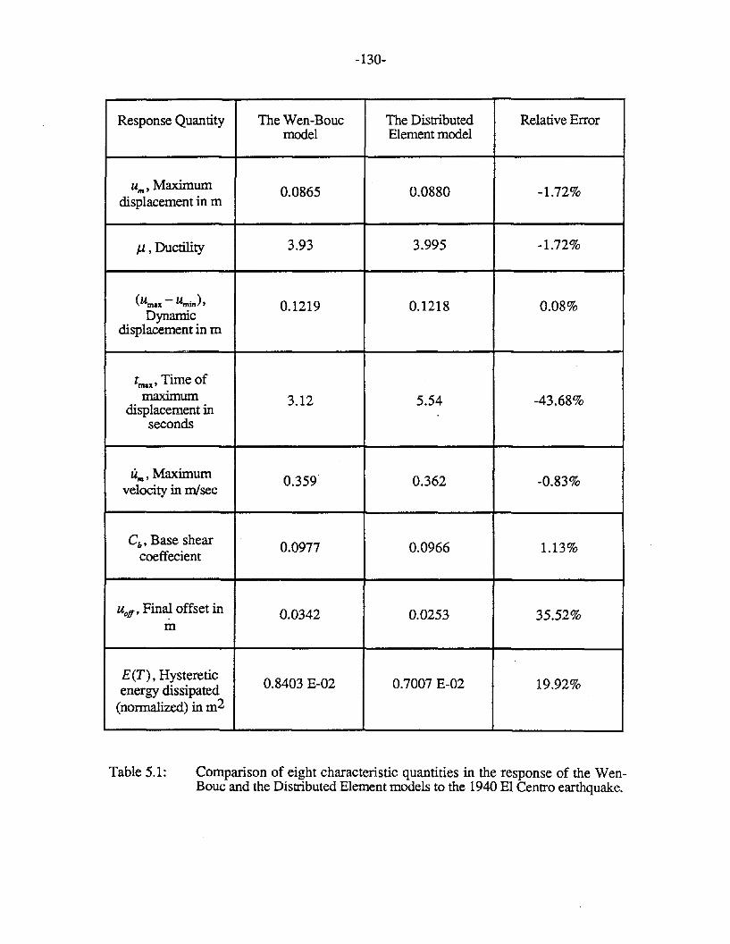
-130-
Response Quantity The Wen-Bouc The Distributed Relative Errormodel Element model
u""Maximum 0.0865 0.0880 -1.72%displacement in m
J1. , Ductility 3.93 3.995 -1.72%
(umax - umin ), 0.1219 0.1218 0.08%Dynamic
displacement in m
tmax ' Time ofmaximum 3.12 5.54 -43.68%
displacement inseconds
u""Maximum 0.359 0.362 -0.83%velocity in m/sec
Cb , Base shear 0.0977 0.0966 1.13%coeffecient
uoff ' Fin~ offset in 0.0342 0.0253 35.52%m
E(T), Hysteretic0.8403 E-02 0.7007 E-02 19.92%energy dissipated
(normalized) in m2
Table 5.1: Comparison of eight characteristic quantities in the response of the WenBouc and the Distributed Element models to the 1940 El Centro earthquake.
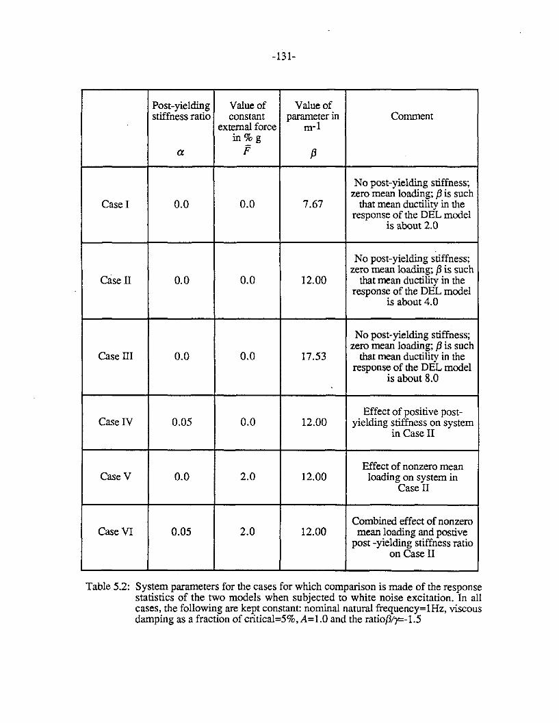
-131-
Post-yielding Value of Value ofstiffness ratio constant parameter in Comment
external force m-1in%g
a F f3
No post-yielding stiffness;zero mean loading; f3 is such
Case I 0.0 0.0 7.67 that mean ductility in theresponse of the DEL model
is about 2.0
No post-yielding stiffness;zero mean loading; f3 is such
Case II 0.0 0.0 12.00 that mean ductility in theresponse of the DEL model
is about 4.0
No post-yielding stiffness;zero mean loading; f3 is such
Case III 0.0 0.0 17.53 that mean ductility in theresponse of the DEL model
is about 8.0
Effect of positive post-Case IV 0.05 0.0 12.00 yielding stiffness on system
in Case II
Effect of nonzero meanCase V 0.0 2.0 12.00 loading on system in
Case II
Combined effect of nonzeroCase VI 0.05 2.0 12.00 mean loading and postive
post -yielding stiffness ratioon Case II
Table 5.2: System parameters for the cases for which comparison is made of the responsestatistics of the two models when subjected to white noise excitation. In allcases, the following are kept constant: nominal natural frequency=IHz, viscousdamping as a fraction of critical=5%, A=1.0 and the ratiof3!)=-1.5
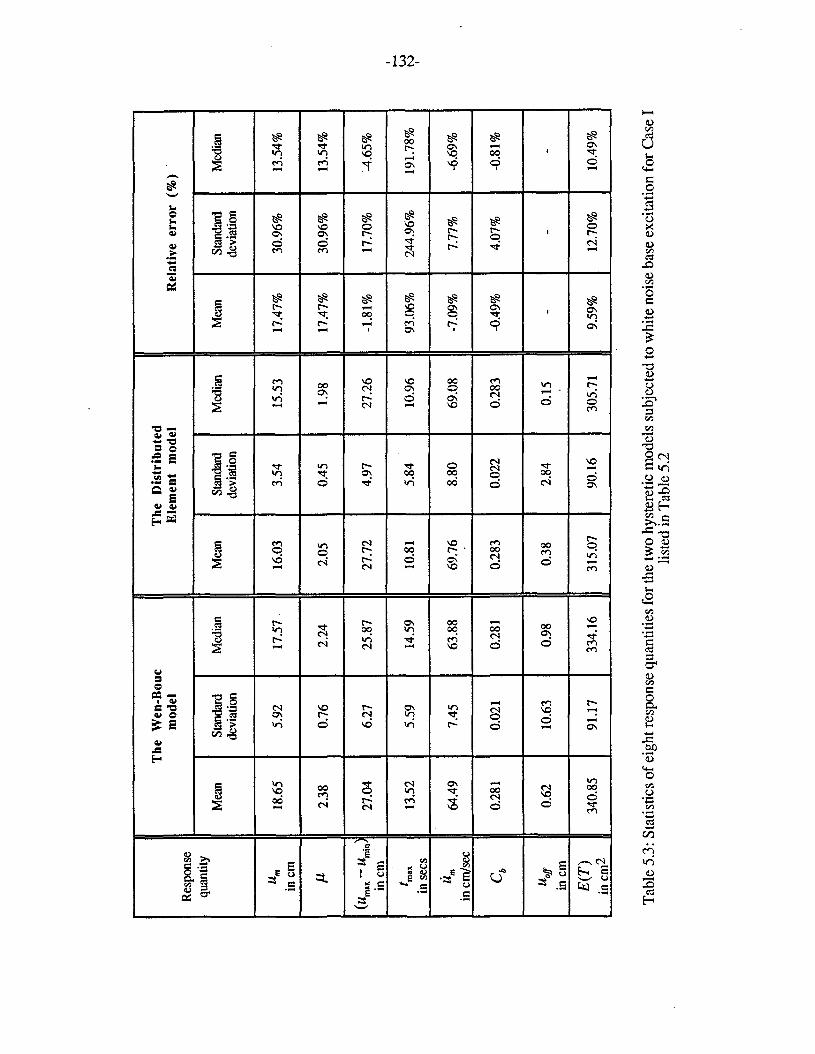
The
Wen
-Bou
eT
heD
istr
ibut
edm
odel
Ele
men
tm
odel
Rel
ativ
eer
ror
(%)
.R
espo
nse
quan
tity
Mea
nSt
anda
rdM
edia
nM
ean
Stan
dard
Med
ian
Mea
nSt
anda
rdM
edia
nde
viat
ion
devi
atio
nde
viat
ion
u m18
.65
5.92
17.5
716
.03
3.54
15.5
317
.47%
30.9
6%13
.54%
inem J1
2.38
0.76
2.24
2.05
0.45
1.98
17.4
7%30
.96%
13.5
4%
(um
ax-
Um
in27
.04
6.27
25.8
727
.72
4.97
27.2
6-1
.81%
17.7
0%'-4
.65%
inem
t max
13.5
25.
5914
.59
10.8
15.
8410
.96
93.0
6%24
4.96
%19
1.78
%in
sees
u m64
.49
7.45
63.8
869
.76
8.80
69.0
8-7
.09%
7.77
%-6
.69%
inem
/sec
C b0.
281
0.02
10.
281
0.28
30.
022
0.28
3-0
.49%
4.07
%-0
.81%
Uo
jf0.
6210
.63
0.98
0.38
2.84
0.15
--
-in
em
E(T)
340.
859
U7
334.
1631
5.07
90.1
630
5.71
9.59
%12
.70%
10.4
9%in
em2
Tab
le5.
3:St
atis
tics
ofei
ghtr
espo
nse
quan
titie
sfo
rth
etw
ohy
ster
etic
mod
els
subj
ecte
dto
whi
teno
ise
base
exci
tatio
nfo
rC
ase
Ilis
ted
inT
able
5.2
I .......
w tv I
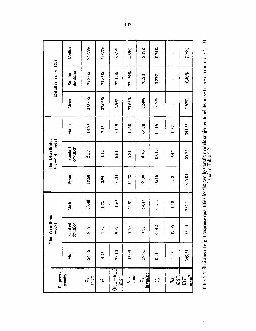
The
Wen
-Bou
eT
he
Dis
trib
ute
dm
odel
Ele
men
tm
odel
Rel
ativ
eer
ror
(%)
Res
pons
equ
antit
yM
ean
Stan
dard
Med
ian
Mea
nSt
anda
rdM
edia
nM
ean
Stan
dard
Med
ian
devi
atio
nde
viat
ion
devi
atio
n
u m24
.56
9.39
23.4
819
.60
5.57
18.5
727
.06%
37.8
3%24
.65%
inem J1
4.93
1.89
4.72
3.94
1.12
3.73
27.0
6%37
.83%
24.6
5%
(um
ax-u
min
33.1
09.
3731
.67
31.0
36.
6130
049
7.26
%22
.42%
'3.3
1%in
em
t max
13.9
95.
4014
.91
11.7
85.
8112
.50
75.6
8%22
1.59
%4.
89%
inse
es
U m59
.91
7.23
59.4
265
.08
8.26
64.7
8-7
.59%
7.18
%-8
.17%
inem
/sec
C b0.
214
0.01
20.
214
0.21
60.
012
0.21
6-0
.74%
3.23
%-0
.74%
u ojf
1.03
17.0
6lA
O1.
1270
440.
37-
--
inem
E(T)
369.
5185
.00
362.
9434
6.83
87.3
634
1.55
7.62
%10
.40%
'7.
96%
inem
2
Tab
le5.
4:St
atis
tics
ofei
ghtr
espo
nse
quan
titie
sfo
rth
etw
ohy
ster
etic
mod
els
subj
ecte
dto
whi
teno
ise
base
exci
tatio
nfo
rC
ase
IIlis
ted
inT
able
5.2
I ..... w W I
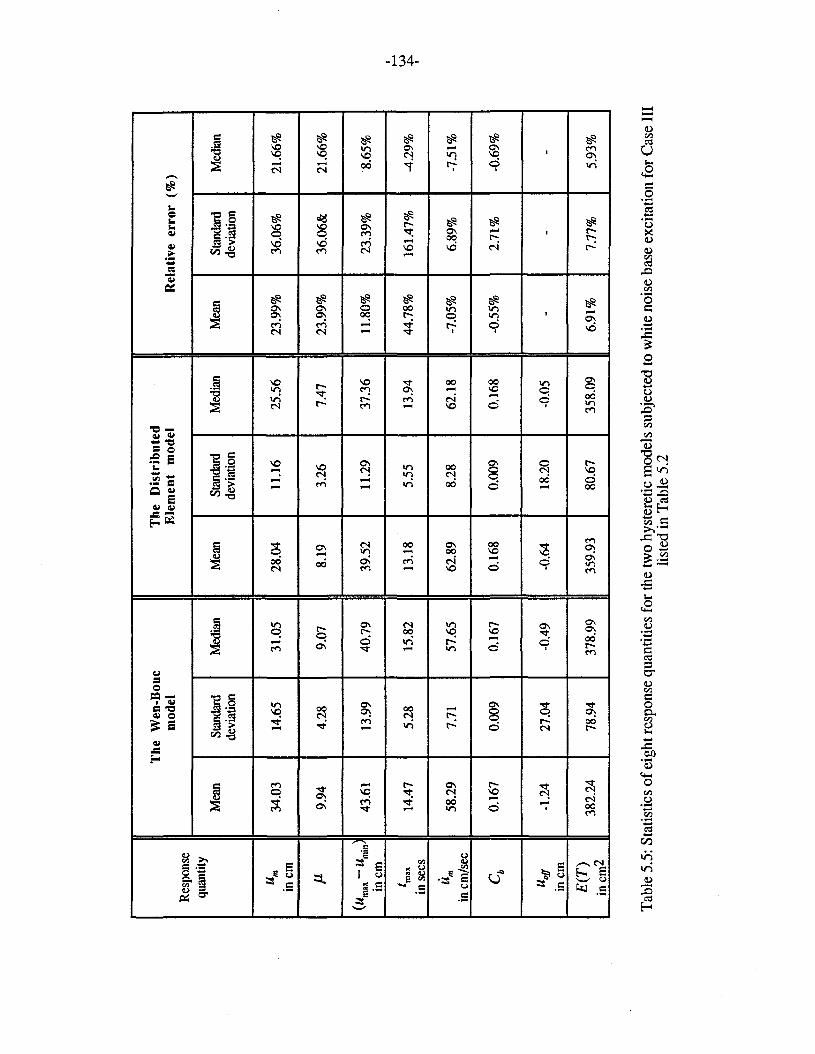
The
Wen
-Bou
eT
heD
istr
ibut
edm
odel
Ele
men
tm
odel
Rel
ativ
eer
ror
(%)
Res
pons
equ
antit
yM
ean
Stan
dard
Med
ian
Mea
nSt
anda
rdM
edia
nM
ean
Stan
dard
Med
ian
devi
atio
nde
viat
ion
devi
atio
n
u m34
.03
14.6
531
.05
28.0
411
.16
25.5
623
.99%
36.0
6%21
.66%
inem JL
9.94
4.28
9.07
8.19
3.26
7.47
23.9
9%36
.06&
21.6
6%
(Um
u-u
min
43.6
113
.99
40.7
939
.52
11.2
937
.36
11.8
0%23
.39%
'8.6
5%in
em
t max
14.4
75.
2815
.82
13.1
85.
5513
.94
44.7
8%16
1.47
%-4
.29%
inse
es
u m58
.29
7.71
57.6
562
.89
8.28
62.1
8-7
.05%
6.89
%-7
.51%
inem
/sec
C b0.
167
0.00
90.
167
0.16
80.
009
0.16
8-0
.55%
2.71
%-0
.69%
u ojf
-1.2
427
.04
-0.4
9-0
.64
18.2
0-0
.05
--
-in
em
E(T)
382.
2478
.94
378.
9935
9.93
80.6
735
8.09
6.91
%7.
77%
5.93
%in
em2
Tab
le5.
5:S
tati
stic
so
feig
htre
spon
sequ
anti
ties
for
the
two
hyst
eret
icm
odel
ssu
bjec
ted
tow
hite
nois
eba
seex
cita
tion
for
Cas
eII
Ili
sted
inT
able
5.2
I ......
w +:>-
I
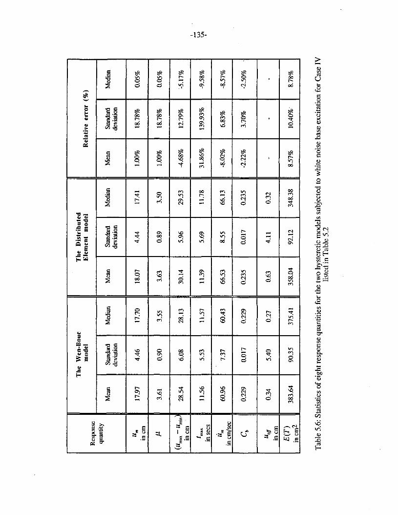
Th
eW
en-B
oue
Th
eD
istr
ibu
ted
mod
elE
lem
ent
mod
elR
elat
ive
erro
r(%
)R
espo
nse
quan
tity
Mea
nSt
anda
rdM
edia
nM
ean
Stan
dard
Med
ian
Mea
nSt
anda
rdM
edia
nde
viat
ion
devi
atio
n'd
evia
tion
u m17
.97
4.46
17.7
018
.07
4.44
17.4
11.
00%
18.7
8%0.
05%
inem J1
3.61
0.90
3.55
3.63
0.89
3.50
1.00
%18
.78%
0.05
%
(Um
ax-
u min
\28
.54
6.08
28.1
330
.14
5.96
29.5
3-4
.68%
12.7
9%'-5
.17%
inem
t ma
x11
.56
5.53
11.5
711
.39
5.69
11.7
831
.86%
139.
93%
-9.5
8%in
sees
U m60
.96
7.37
60.4
366
.53
8.55
66.1
3-8
.02%
6.83
%-8
.57%
inem
/sec
C b0.
229
0.Q
170.
229
0.23
50.
017
0.23
5-2
.22%
3.70
%-2
.50%
uo./f
0.34
5.40
0.27
0.63
4.11
0.32
--
-in
em
E(T)
383.
6490
.35
375.
4135
8.04
92.1
234
8.38
8.57
%10
.40%
8.78
%in
em2
Tab
le5.
6:S
tati
stic
so
feig
htre
spon
sequ
anti
ties
for
the
two
hyst
eret
icm
odel
ssu
bjec
ted
tow
hite
nois
eba
seex
cita
tion
for
Cas
eIV
list
edin
Tab
le5.
2
I ......
w VI
I
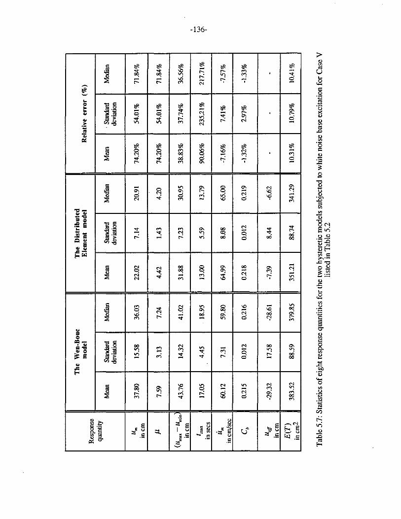
Th
eW
en-B
oue
Th
eD
istr
ibu
ted
mod
elE
lem
ent
mod
elR
elat
ive
erro
r(%
)R
espo
nse
quan
tity
Mea
nSt
anda
rdM
edia
nM
ean
Stan
dard
Med
ian
Mea
n.S
tand
anI
Med
ian
devi
atio
nde
viat
ion
devi
atio
n
u m37
.80
15.5
836
.03
22.0
27.
1420
.91
74.2
0%54
.01%
71.8
4%in
em J17.
593.
137.
244.
421.
434.
2074
.20%
54.0
1%71
.84%
(Um
ax-
umin~
43.7
614
.32
41.0
231
.88
7.23
30.9
538
.83%
37.7
4%36
.56%
inem
t lnn
17.0
54.
45.
18.9
513
.00
5.59
13.7
990
.06%
235.
21%
217.
71%
inse
es
U m60
.12
7.31
59.8
064
.99
8.08
65.0
0-7
.16%
7.41
%-7
.57%
inem
/sec
C b0.
215
0.01
20.
216
0.21
80.
012
0.21
9-1
.32%
2.97
%-1
.33%
u ojf
-29.
3217
.58
-28.
61-7
.39
8.44
-6.6
2-
--
inem
E(T
)38
3.52
88.5
937
9.85
351.
2188
.74
341.
2910
.31%
10.7
9%10
.41%
inem
2
Tab
le5.
7:St
atis
tics
ofei
ghtr
espo
nse
quan
titie
sfo
rth
etw
ohy
ster
etic
mod
els
subj
ecte
dto
whi
teno
ise
base
exci
tatio
nfo
rC
ase
Vlis
ted
inT
able
5.2
I ......
w 0\
I
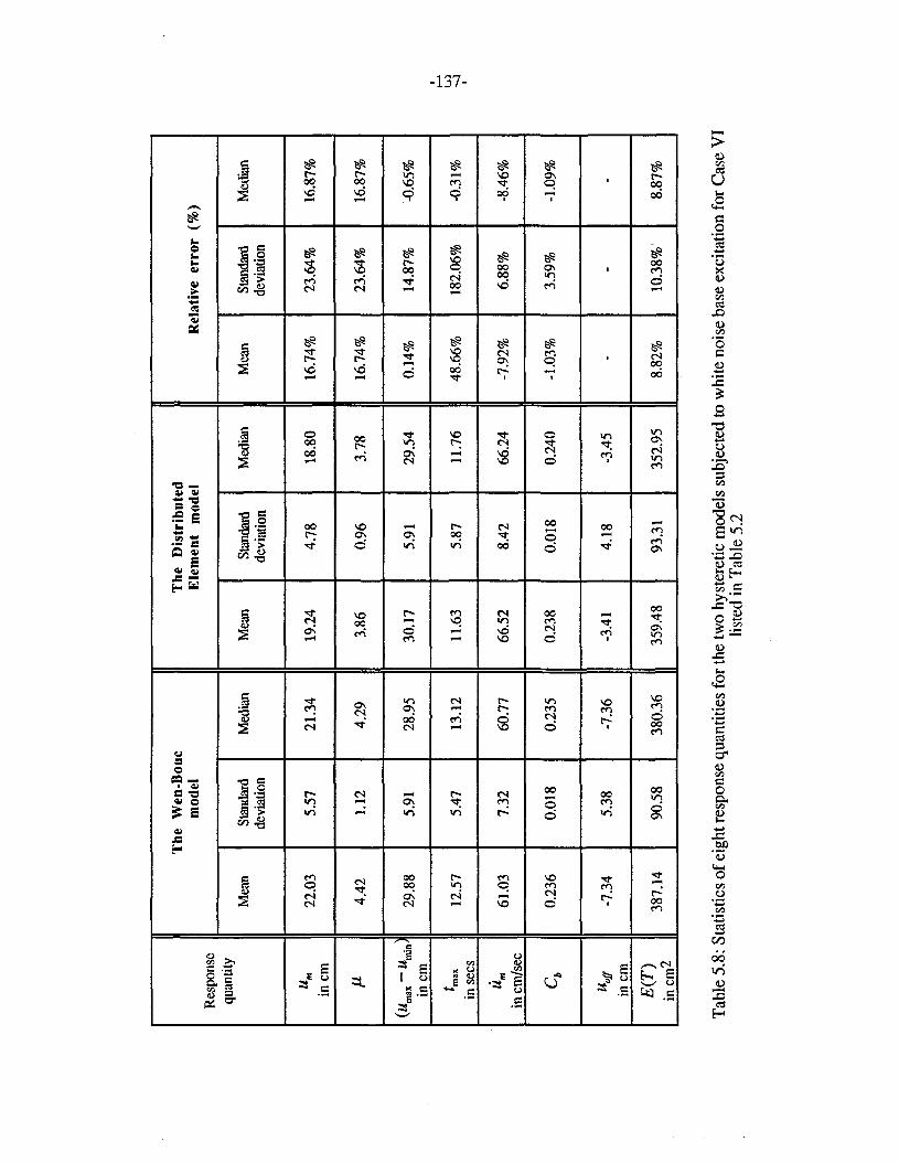
Th
eW
en-B
ou
eT
he
Dis
trib
ute
dm
odel
Ele
men
tm
odel
Rel
ativ
eer
ror
(%)
Res
pons
equ
antit
yM
ean
Stan
dard
Med
ian
Mea
nSt
anda
nlM
edia
nM
ean
Stan
dard
Med
ian
devi
atio
nde
viat
ion
devi
atio
n
u m22
.03
5.57
21.3
419
.24
4.78
18.8
016
.74%
23.6
4%16
.87%
inem Jl
4.42
1.12
4.29
3.86
0.96
3.78
16.7
4%23
.64%
16.8
7%
(Um
ax-
u min
29.8
85.
9128
.95
30.1
75.
9129
.54
0.14
%14
.87%
'-0.6
5%in
em t max
12.5
75.
4713
.12
11.6
35.
8711
.76
48.6
6%18
2.06
%-0
.31%
inse
es
u m61
.03
7.32
60.7
766
.52
8.42
66.2
4-7
.92%
6.88
%-8
.46%
inem
/sec
Cb
0.23
60.
Ql8
0.23
50.
238
0.01
80.
240
-1.0
3%3.
59%
-1.0
9%
Uof
/-7
.34
5.38
-7.3
6-3
.41
4.18
-3.4
5-
--
inem
E(T
)38
7.14
90.5
838
0.36
359.
4893
.31
352.
958.
82%
10.3
8%'
8.87
%in
em2
Tab
le5.
8:St
atis
tics
ofei
ghtr
espo
nse
quan
titie
sfo
rth
etw
ohy
ster
etic
mod
els
subj
ecte
dto
whi
teno
ise
base
exci
tatio
nfo
rC
ase
VI
liste
din
Tab
le5.
2
I .......
w -.] I
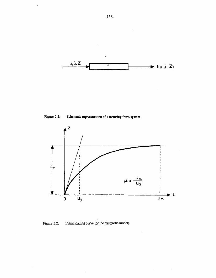
Figure 5.1:
-138-
__u_,U_,Z~.J f I---~"~ f(u,u, Z)
Schematic representation of a restoring force system.
z
o Uy
u}J- - m-uy
UmU
Figure 5.2: Initial loading curve for the hysteretic models.
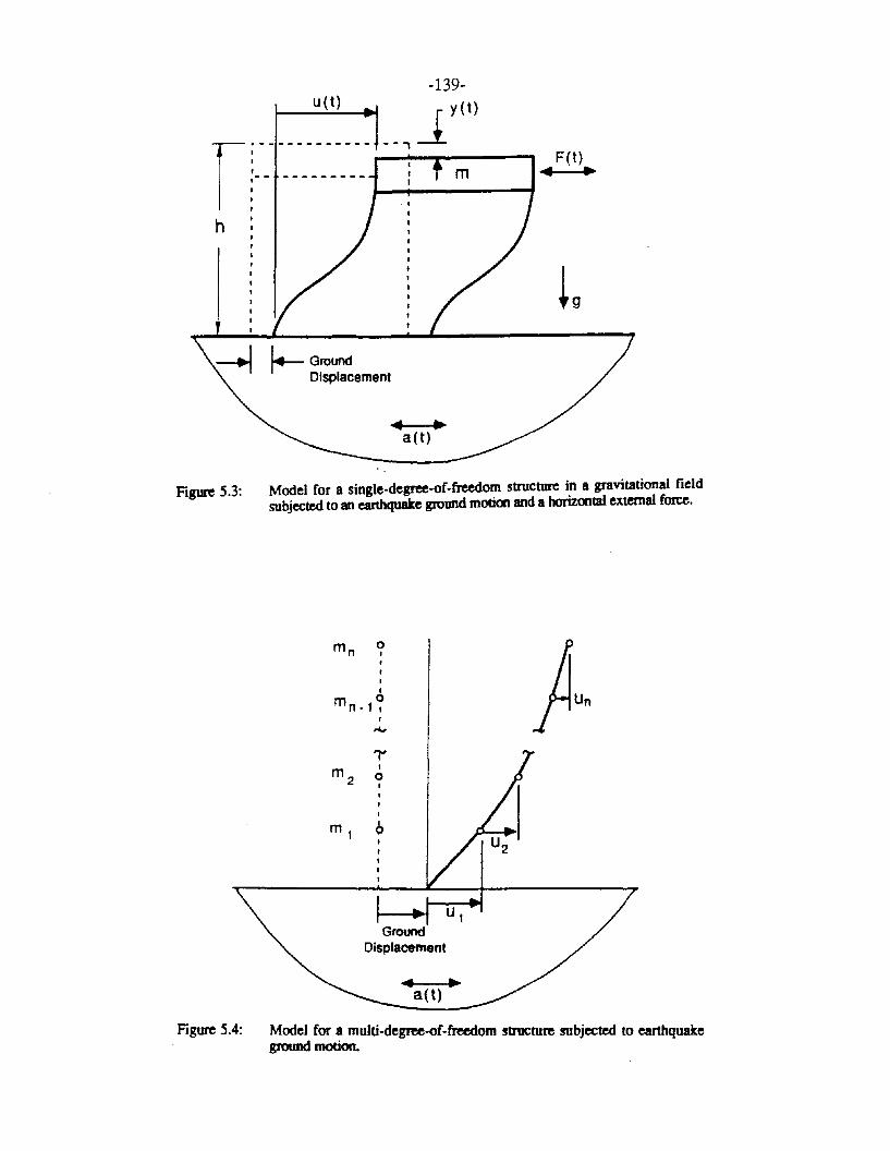
~g
F(t}. ..m
• •a (t)
-139
__ ,-.ly(tlu(t)
j.- GroundDisplacement
hf r------------
,- - - - - - - - -- -: .....--.-------f
Figure 5.3: Model for a single-degree-of-freedom structure in a gravitational fieldsubjected to an earthquake ground motion and a horizontal external force.
mn 9,I
I
I
mn_1~I
.v
m 1
GroundDisplacement. ..
a(t)
Figure 5.4: Model for ~ multi-degree-of-freedom structure subjected to earthquakeground motton.
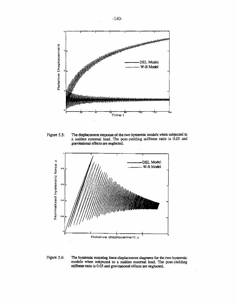
-140-
4,----...,.----,----,----...,.----,-----,,------,
...CQ) 3
EQ)ottla.IIIoQ)>;::t1lQi[!
Figure 5.5:
NQ)
~ 0.8
o...oi...Q) 06...Ul>..c"0Q) 0.4
.~(ijE...o 0.2Z
Figure 5.6:
.•.,~y.'fJ.\~ ...
~~VJ(tr:'I ...
~,. '_.'p"n
I 'If ,I
,.hU.'.:.....:;.'tf' '. l!~t~"
.,••••~';ll"' •.hm--~"I :;:If'i.
---DEL Model---W-B Model
Timet
The displacement response of the two hysteretic models when subjected toa sudden external load. The post-yielding stiffness ratio is 0.05 andgravitational effects are neglected.
---DEL Model----W-B Model
4
Relative displacement u
The hysteretic restoring force-displacement diagrams for the two hystereticmodels when subjected to a sudden external load. The post-yieldingstiffness ratio is 0.05 and gravitational effects are neglected.
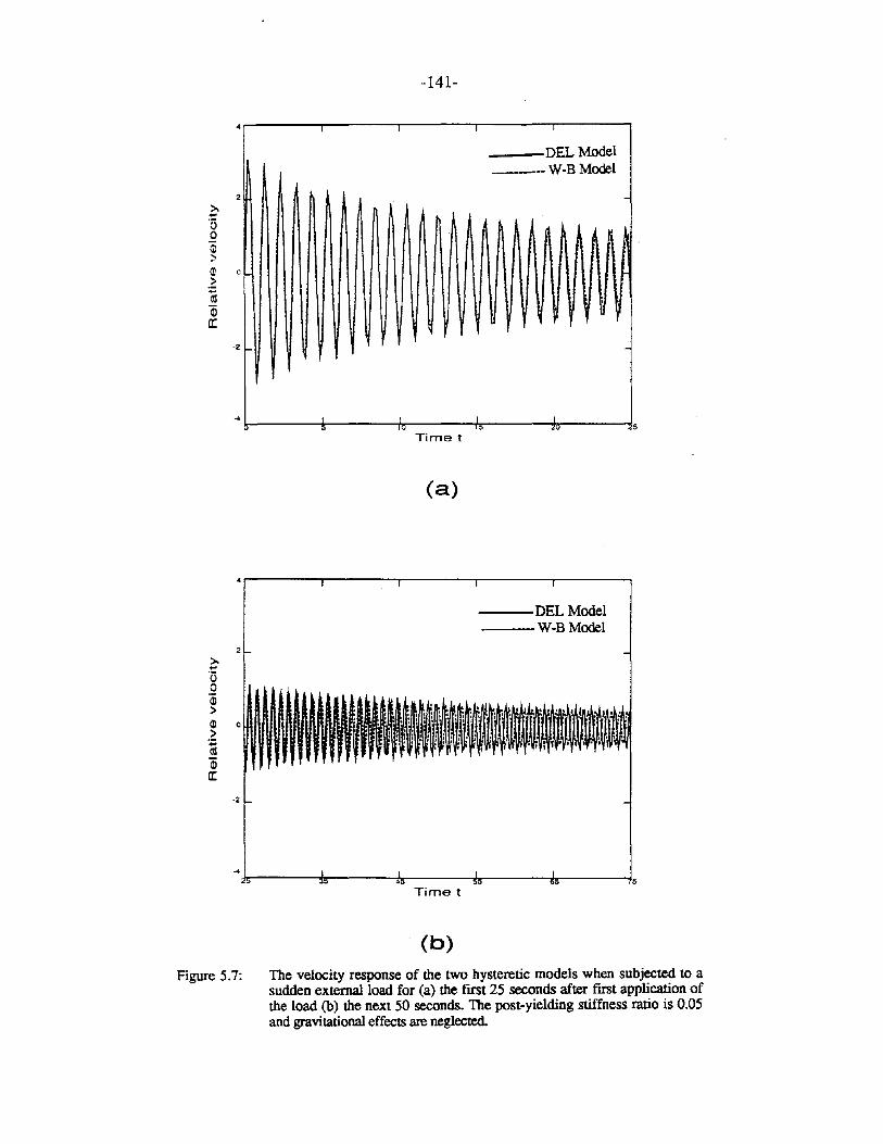
-141-
___DEL Model__W-BModel
2
-2
!I-----+------,~---__J.r.---___.l,..._--___.ls
Time t
(a)
4r----,-----r-----,-------,r--------,
---DEL Model---W-B Model
2
>....·0o~>(]) a>;:(l1
~a:
·2
-4:1s----,r-------:k-----.b------.h.------JsTime t
(b)
Figure 5.7: The velocity response of the two hysteretic models when subjected to asudden external load for (a) the fIrst 25 seconds after fIrst application ofthe load (b) the next 50 seconds. The post-yielding stiffness ratio is 0.05and gravitational effects are neglected.
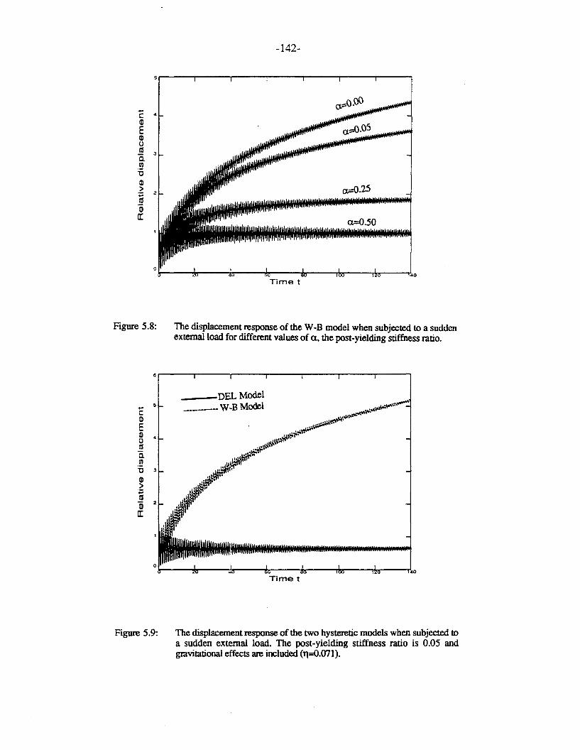
C 4
Q)
EQ)ocaa. 3
.!!l'0Q)
.~ 2
;OJcr
Figure 5.8:
-142-
a.=0.25
0.=0.50
/r---..;"...--""*r---b;---,l,..-----.lv.----r!m-----T.4oTime t
The displacement response of the W-B model when subjected to a suddenexternal load for different values of a, the post-yielding stiffness ratio.
6,..----..,..----,-----r---.....,.---r----.,.-------,
5..c:Q)
EQ) 4ocaa.(I)
'0 3
Q)>:;::ca
OJ 2
cr
__-DEL Model_____- W-B Model
Jr----.,j"---...,1"---....",,.----,j.,.----~1.o._----,rl,,._-___T.,40
Timet
Figure 5.9: The displacement response of the two hysteretic models when subjected toa sudden external load. The post-yielding stiffness ratio is 0.05 andgravitational effects are included (,,=0.071).
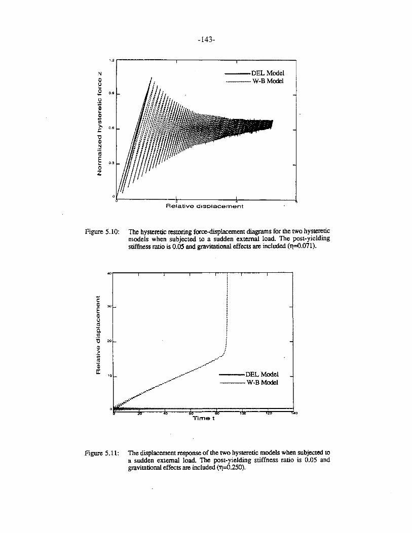
-143-
1.2 r--------.-------,----------.
N
illo....E 09
o:;Ql...Ql...(/l
>. 0.6~
'CQlN
iE 03oZ
---DEL Model---W-B Model
Relative displacement
Figure 5.10: The hysteretic restoring force-displacement diagrams for the two hystereticmodels when subjected to a sudden external load. The post-yieldingstiffness ratio is 0.05 and gravitational effects are included ('11=0.071).
10
·ooooo
·ooooo
o
o·ooo·
~---~...-.-~-_...~. ---DEL Model..,..."..
.,,/ W-BModel--~.,...-,"-../.,..1." .....
o~~=:==;r;;:::===;~::::;+;:==;~::::;tF 40
...cQl 30
EQlotoa.(/l
:0 20
Ql>:;toil!
Time t
Figure 5.11: The displacement response of the two hysteretic models when subjected toa sudden external load. The post-yielding stiffness ratio is 0.05 andgravitational effects are included ('11=0.250).
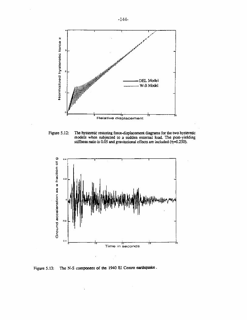
NQ)
e,g 3
o:;::Q)...Q)...III>. 2.r:'CQ)N
(UE...oZ
-144-
---DEL Model----WeB Model
&------T------+rr-------h:-----~oRelative displacement
Figure 5.12: The hysteretic restoring force-displacement diagrams for the two hystereticmodels when subjected to a sudden external load. The post-yieldingstiffness ratio is 0.05 and gravitational effects are included (11=0.250).
Cl 0.4...0c:0:;:;0t1l 0.2......t1lent1lc:0:;::t1l...Q)Qj00t1l ·0.2
'Cc::::l0...(9
·040
Time in seconds
Figure 5.13: The N-S component of the 1940 El Centro earthquake.
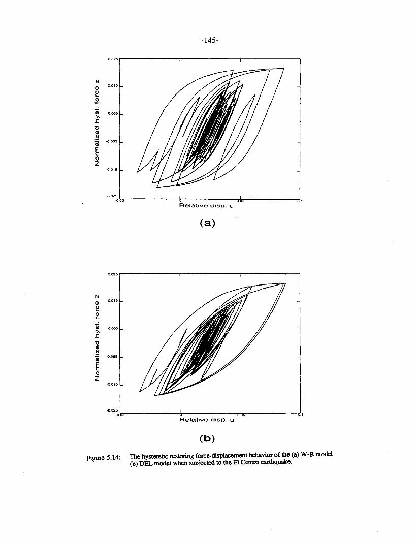
-145-
0.025
NQ)
0.015
0..0....;CIl 0.005>..r:'0Q)N
(ij "'.005
E..0Z
"'.0'5
·0.025_O.bs-------+--------,rl....---------J.1
Relative disp. u
(a)
0.025
NQ)
0.0'5
0..0....;CIl 0.005>..r:'0Q)N
(ij "'.005
E..0Z
"'.015
-o.02~O,,'o:s--------r-------~:---------.J"
Relative disp. u
(b)
Figure 5.14: The hysteretic restoring force-displacement behavior of the (a) W-B model(b) DEL model when subjected to the El Centro earthquake.
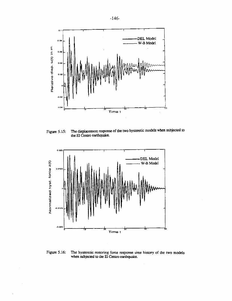
-146-
0.1
DEL Model0.08
----- WeB Model
Ec: 0.06 l.-. "".. ""...,
"J ..0.04 ..
:'a.w .~U 0.02 .Ql \'>:; tftUQj 0
c:-0.02
·0.04 0
Timet
Figure 5.15: The displacement response of the two hysteretic models when subjected tothe EI Centro earthquake.
0.025 I I I
DEL Model.-... ---WeB Model......N
Ql 0.0125 f-
f !
-(J..0
.I I... a..: " i~ I
~(/)
,.~
>. l1il~
,~~.
,.c 0 "
,
'0 'i i'. 1"7, .Ql ' ..~(ijE..0 -0.0125 -Z .·... .·.·.:.
-0.025 I I I
'u . 20 ~u .u 0
Timet
Figure 5.16: The hysteretic restoring force response Lime history of the two modelswhen subjected to the EI Centro earthquake.
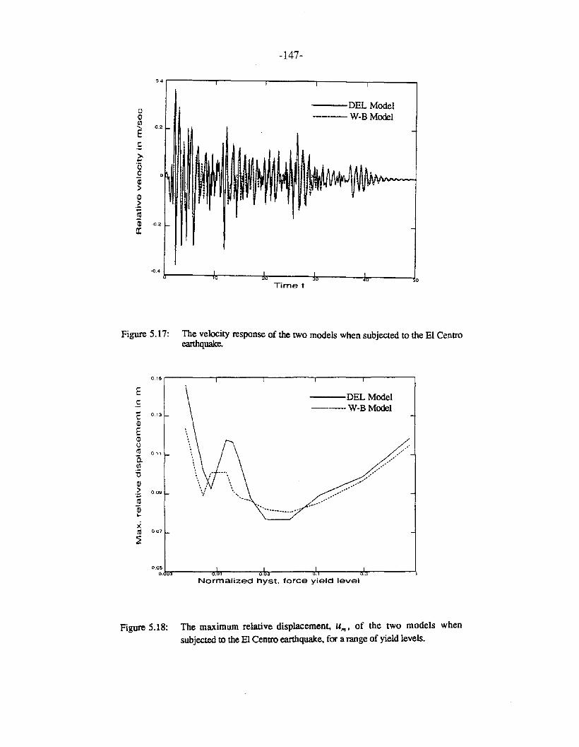
-147-
04 r---l----..,.---~r__---___r_---___.
o
0.2
tlQlI/J.....Et:
>....'0oQi>Ql>;caQi -0.2a:
---DEL Model----W-B Model
-0.4 !r---~r__---*"---~In-----1,,----JoTime t
Figure 5.17: The velocity response of the two models when subjected to the EI Centroearthquake. .
0.15 r__-----r----.------,-----.-------,EcC 013
OJEQltlt1l 0 "
0-W'5Ql> 0.09:;::;11lOJ~
---DEL Model------- W-B Model
xca 0.07
:2
00~.kr----".j-n-----,M,..,.-----.,.!,----.."J.".-------l
Normalized hyst. force yield level
Figure 5.18: The maximum relative displacement, U"., of the two models whensubjected to the EI Centro earthquake, for a range of yield levels.
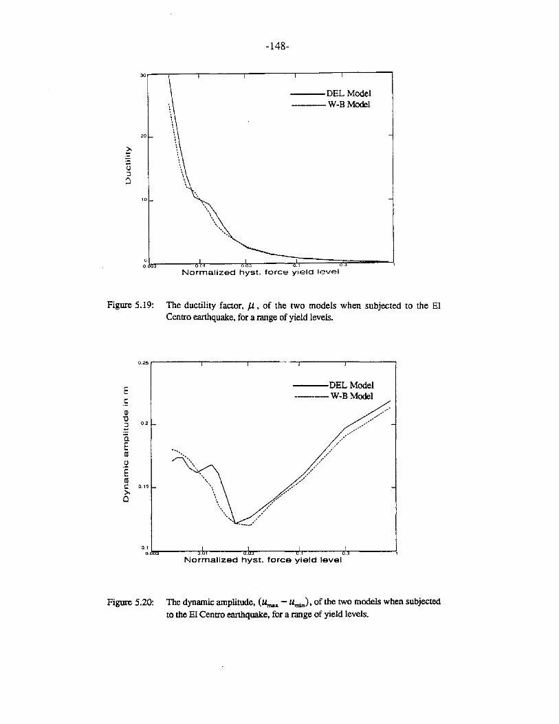
-148-
30..---,..-----,----..,-----r-----r---~
---DEL Model-----W-B Model....
,
,'.
10
20
~..(J::Jo
0l.----,.,-k-----,,-l,.,---=;;L;::::====~=-JoNormalized hyst. force yield level
Figure 5.19: The ductility factor. J.L. of the two models when subjected to the EICentro earthquake, for a range of yield levels.
0.25
EcQ)"0::J 0.2
.'.::Q.
Et1l(.l
Et1lC 0.15
>-0
---DEL Model----W-B Model
0.1o..m-----m!lr-----,rllor-----,r';----""l5':or------\
Normalized hyst. force yield level
Figure 5.20: The dynamic amplitude, (umal< - umin), of the two models when subjectedto the EI Centro earthquake, for a range of yield levels.
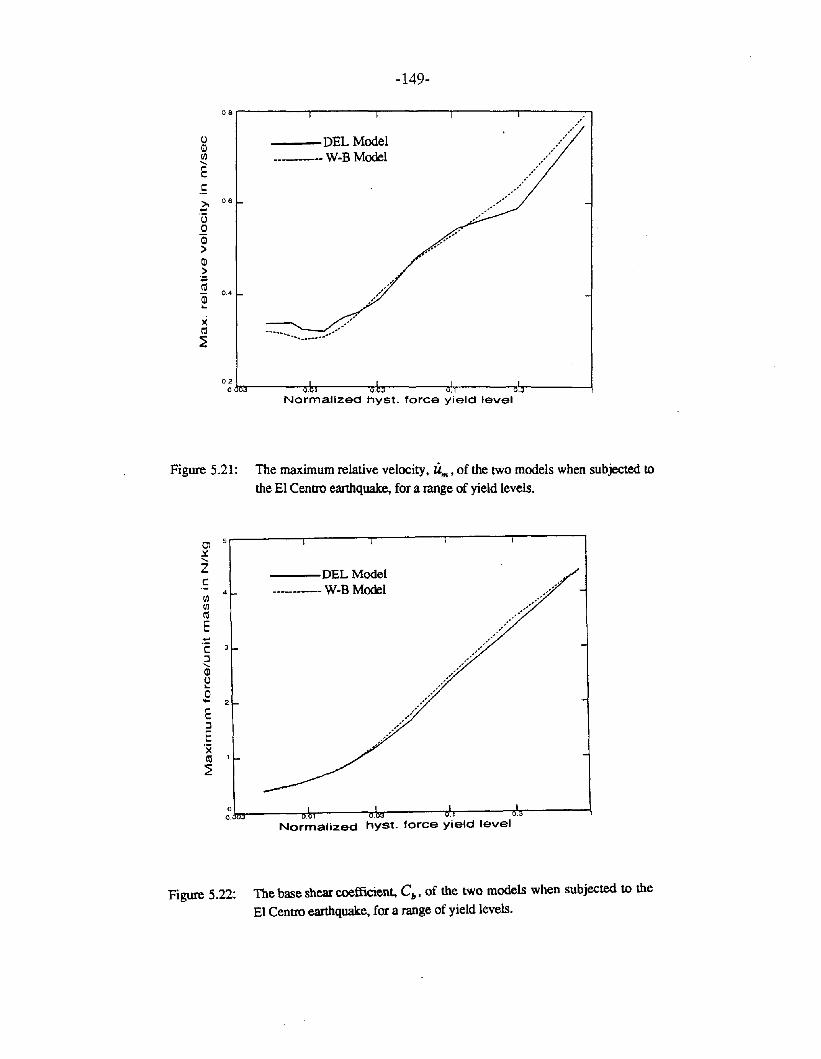
-149-
0.8
C.lQlen.....Ec>. 0.6...'00i>Ql.~;
0.4i'-
X«l~
---DEL Model--W-BModel
.'..............._ ..
Normalized hyst. force y'ield level'
0.2o.6rer---u:lrr----~r:lr.r----c~---"l.,.------t
Figure 5.21: The maximum relative velocity, U"" of the two models when subjected to
the EI Centro earthquake, for a range of yield levels.
...'c 3
::l.....QlC.l'-o...E::l
Ex«l 1
~
Ol~
Zcenen«lE
4
---DEL Model------ W-B Model
Normalized hyst. force yield level~k---~h-r---.......,..4..----~fr-----rn---~
Figure 5.22: The base shear coefficient, Cb' of the two models when subjected to the
El Centro earthquake, for a range of yield levels.
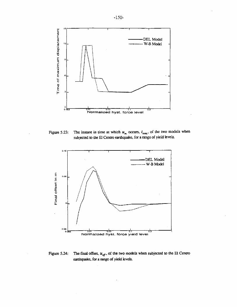
-150-
1Sr-----,----.....----.-----r--------,CQlEQlUettQ.til:0E:J
E'xettE'0Ql
Ei=
12
9
6
3
t.... -----,· '· ', '· ', ,: :, .: t
I \, ., ,, ., .. .. ., ., ,, ,f I
---DEL Model----W-B Model
Normalized hyst. force level~.lil-r---~lrr-----,m-----,,1,-----,.l,,-------1
Figure 5.23: The instant in time at which u", occurs, tmu ' of the two models whensubjected to the El Centro earthquake, for a range of yield levels.
0.12 r------,r----.....----.-----r------,
-----DEL Model------- W-B Model
E0.06
C
...Qltil......0
Ciic[ 0
.0~ ..lil-r----n-lrr-----,m-----,,1,----...,,I.,-----.INormalized hyst. force yield level
Figure 5.24: The final offset., Uoff ' of the two models when subjected to the El Centro
earthquake, for a range of yield levels.
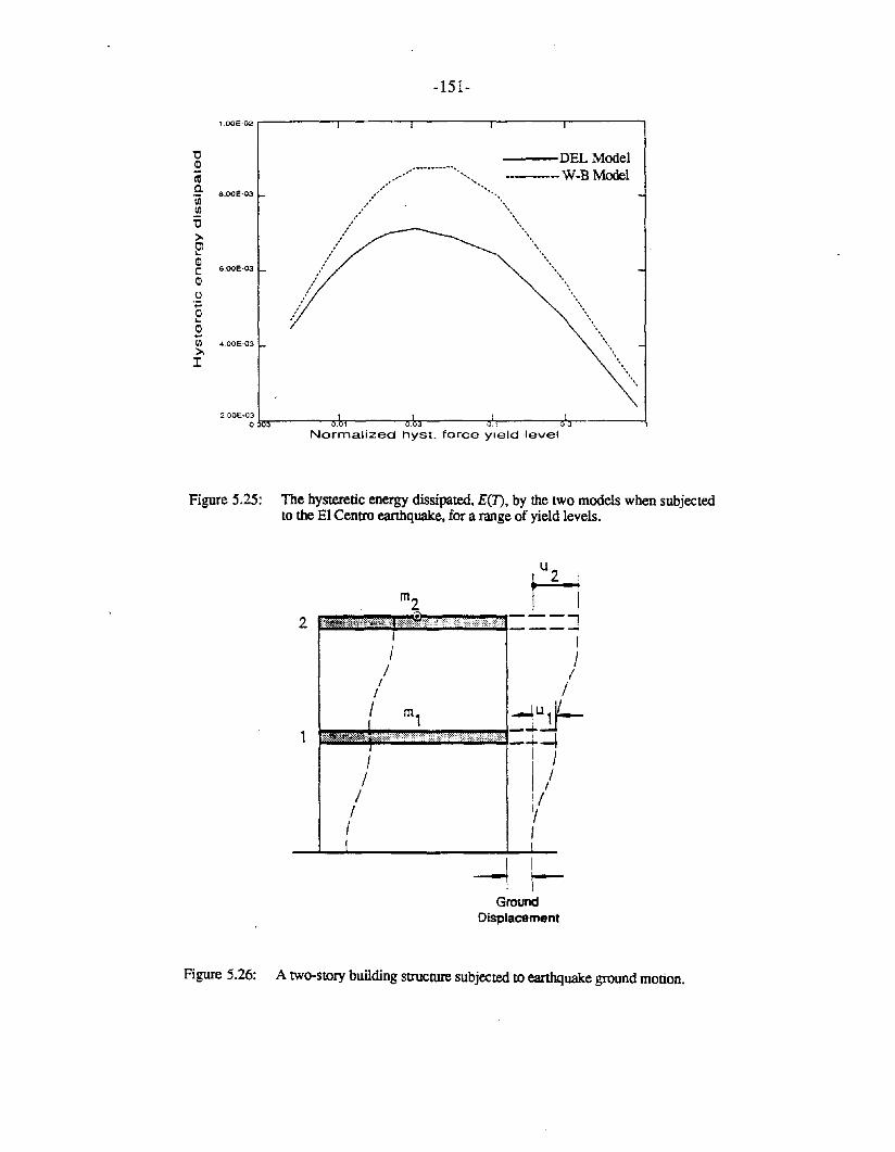
-151-
1.00E-02 ~----r-------r-----r----r-----,
"0~1'IlCo 8.00E-03"iiiUl"0>-OJ'-ill
600E-03Cillu:;:;ill'-ill...Ul 400E-03
>-I
2.00E-O~.k .."..l,-, ...."..j".---__~l,-__----rf-r- -J,
Normalized hyst. force yield level
Figwe 5.25: The hysteretic energy dissipated, £(1), by the two models when subjectedto the EI Centro earthquake, for a range of yield levels.
--1~Ground
Displacement
Figwe 5.26: A two-story building structure subjected to earthquake ground motion.
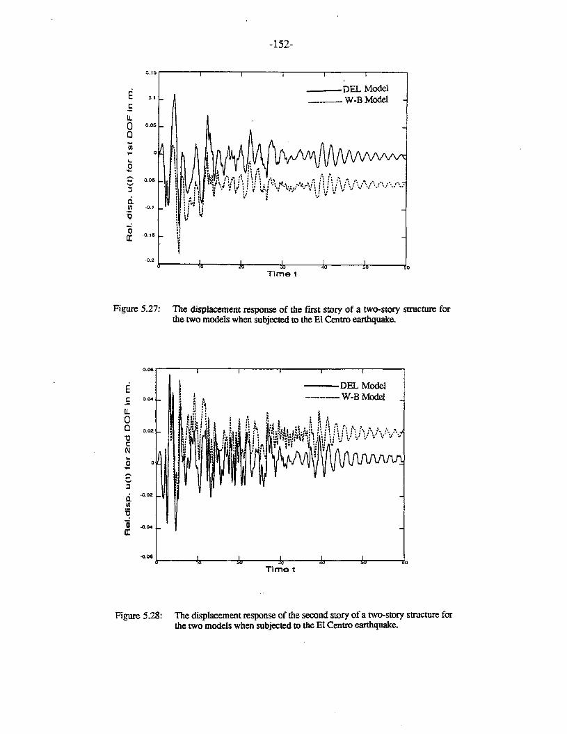
-152-
0.15
E 0.1
c:U.0 0.05
Q...1Il ·... 0 ···... ··0 ··.... ··,... ·-0.05 ·...
I"'":J
ci1Il ·0.1
:ci ....a: -0.15 t:.,..
i-0.2
___DEL Model_______ W-B Model
oTimet
Figure 5.27: The displacement response of the ftrst story of a two-story structure forthe two models when subjected to the EI Centro earthquake.
0.06 r------,------,.-----,.----.......----"'T'"----.,
Ec:U.oQ"0c:(IJ...a....,...........:::l
ciUl:cia:
0.04
0.02
o
·0.02
-0.04
---DEL Model------ W-B Model
-O.06lr-----flJ~---...,b----_.!Ir---__j~---.,!"_---__,!,,
Time t
Figure 5.28: The displacement response of the second story of a two-story structure forthe two models when subjected to the EI Centro earthquake.
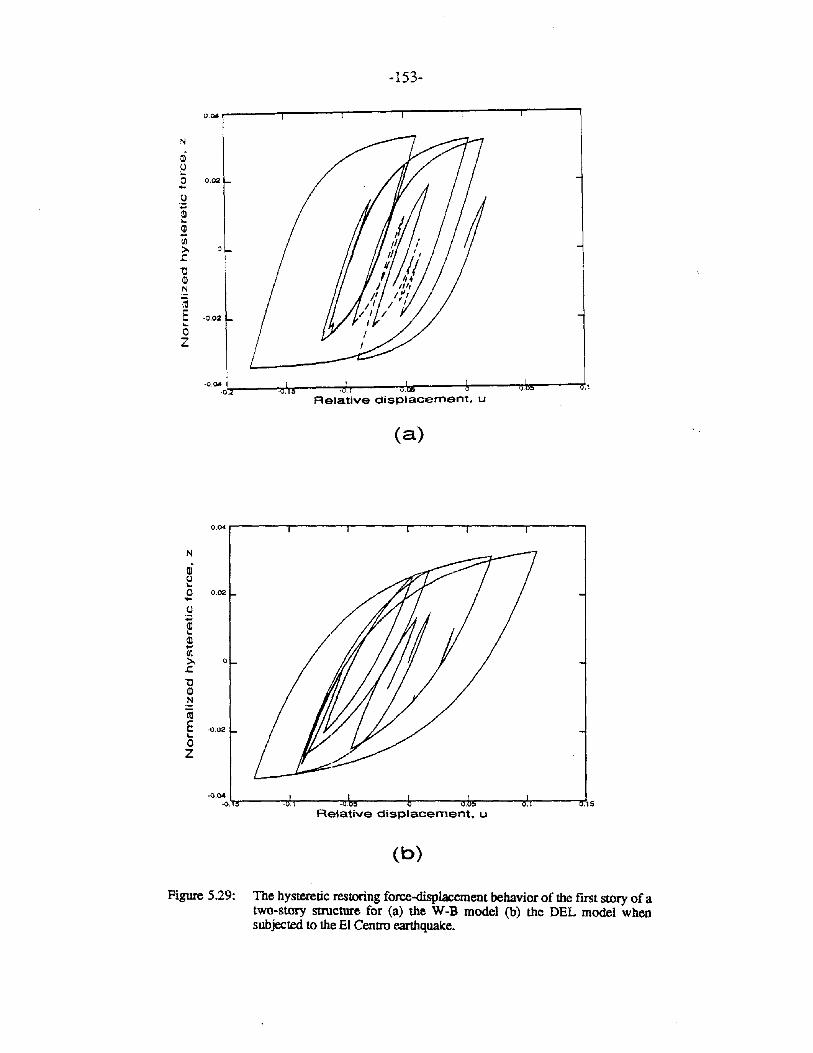
-153-
0.00Il
N
0>(J...2 0.02
~Ql..~rJl>-!:
1:lQ)N
(ijE..0Z
-0.001 .'·0.Relative displacement. u
(a)
0.04
N
oj(J..0 0.02...(J:;:Q)..Q)...III>- 0!:"0Q)N
(ijE ·0.02...0Z
'°o:'o.l.,r----:rf,---~~---lr---<r.b:r_--~r_--ll:'.15Relative displacement, u
(b)
Figure 5.29: The hysteretic restoring force-displacement behavior of the first story of atwo-story structure for (a) the W-B model (b) the DEL model whensubjected to the EI Centto earthquake.
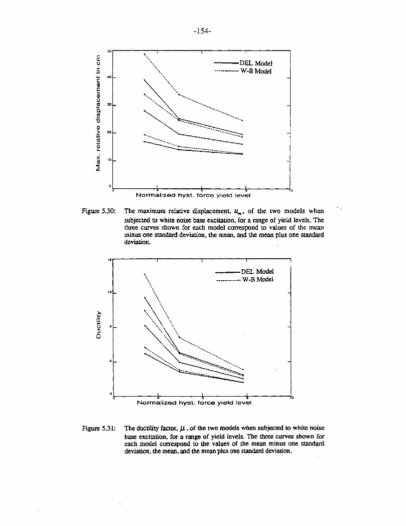
-154-
50
E()
c... 40CQlEQl()ctl 30
C.III:0II)> 20";:;tilQi..x
'0til~
---DEL Model---------- W-B Model
~_._ .._..._..--._._------
or-------;:-------+------+r-------toNormalized hyst. force yield level
Figure 5.30: The maximum relative displacement. u"'. of the two models whensubjected to white noise base excitation, for a range of yield levels. Thethree curves shown for each model correspond to values of the meanminus one standard deviation. the mean. and the mean plus one standarddeviation.
lSr-------,------r-------r-----.,
'2
...() 8
::lo
4
---DEL Model---------- W-B Model
°J,------~:------_l.-----+----~'oNormalized hyst. force yield level
Figure 5.31: The ductility factor, J.L. of the two models when subjected to white noisebase excitation. for a range of yield levels. The three curves shown foreach model correspond to the values of the mean minus one standarddeviation. the mean. and the mean plus one standard deviation.
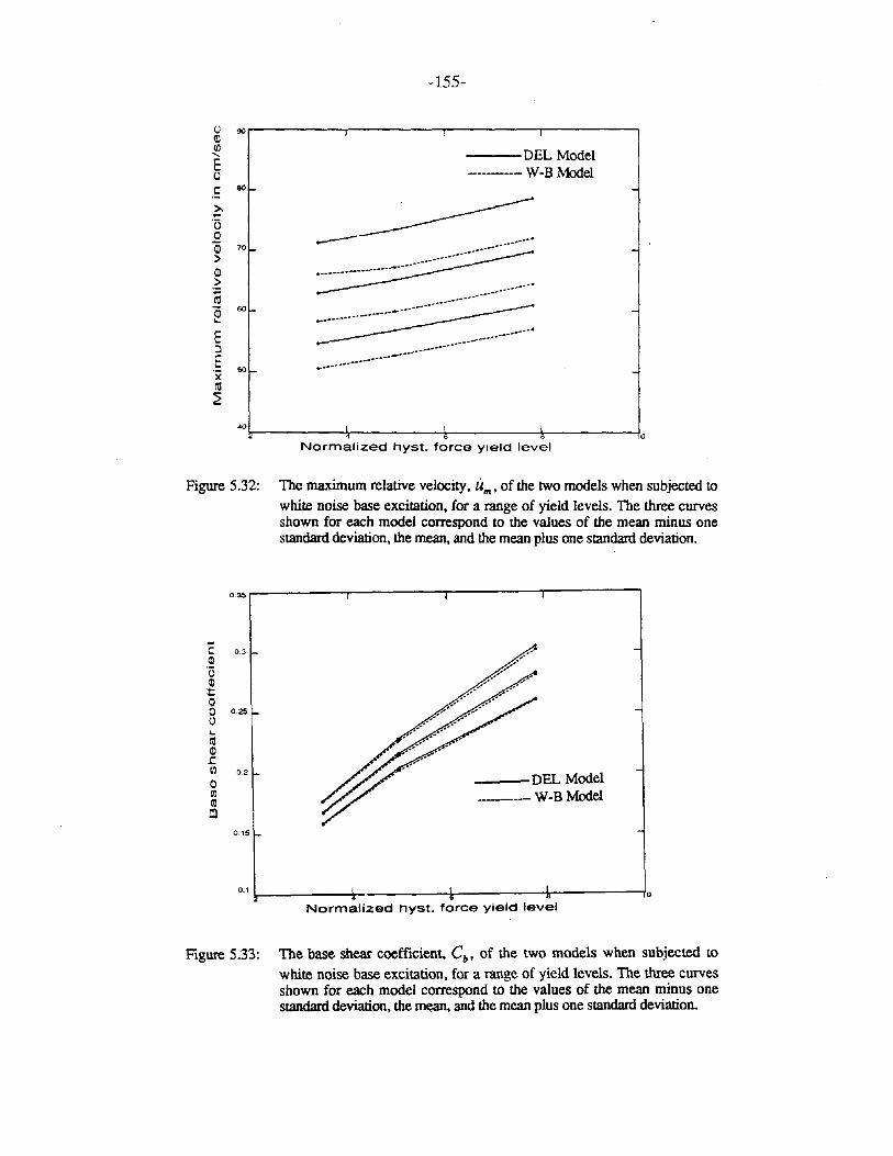
-155-
---DEL Model---------- W-B Model
(,) 9Or--------,-----.....,..-------r-----__Q)III......Euc eo
~.••.........._ _ __•........................•
---------------==._ _ ......- , -.- - -.., --.
E:::l
E 50XCIl~
~·13oQi 70
>Q)>+=CIlQi 60"-
4°1,--------!Jr------4------lr--------J0
Normalized hyst. force yield level
Figure 5.32: The maximum relative velocity, U"" of the two models when subjected to
white noise base excitation, for a range of yield levels. The three curvesshown for each model correspond to the values of the mean minus onestandard deviation, the mean, and the mean plus one standard deviation.
0.35
-c: 0.3
ill"C:iill~ill0 0.25(,)
"-CIlill.J:til 02
DEL ModelillIII _______ W-B ModelellCD
0.15
0.1 L--------!.-------l,-----+-----IoNormalized hyst. force yield level
Figure 5.33: The base shear coefficient. Cb , of the two models when subjected to
white noise base excitation, for a range of yield levels. The three curvesshown for each model correspond to the values of the mean minus onestandard deviation, the mean, and the mean plus one standard deviation.
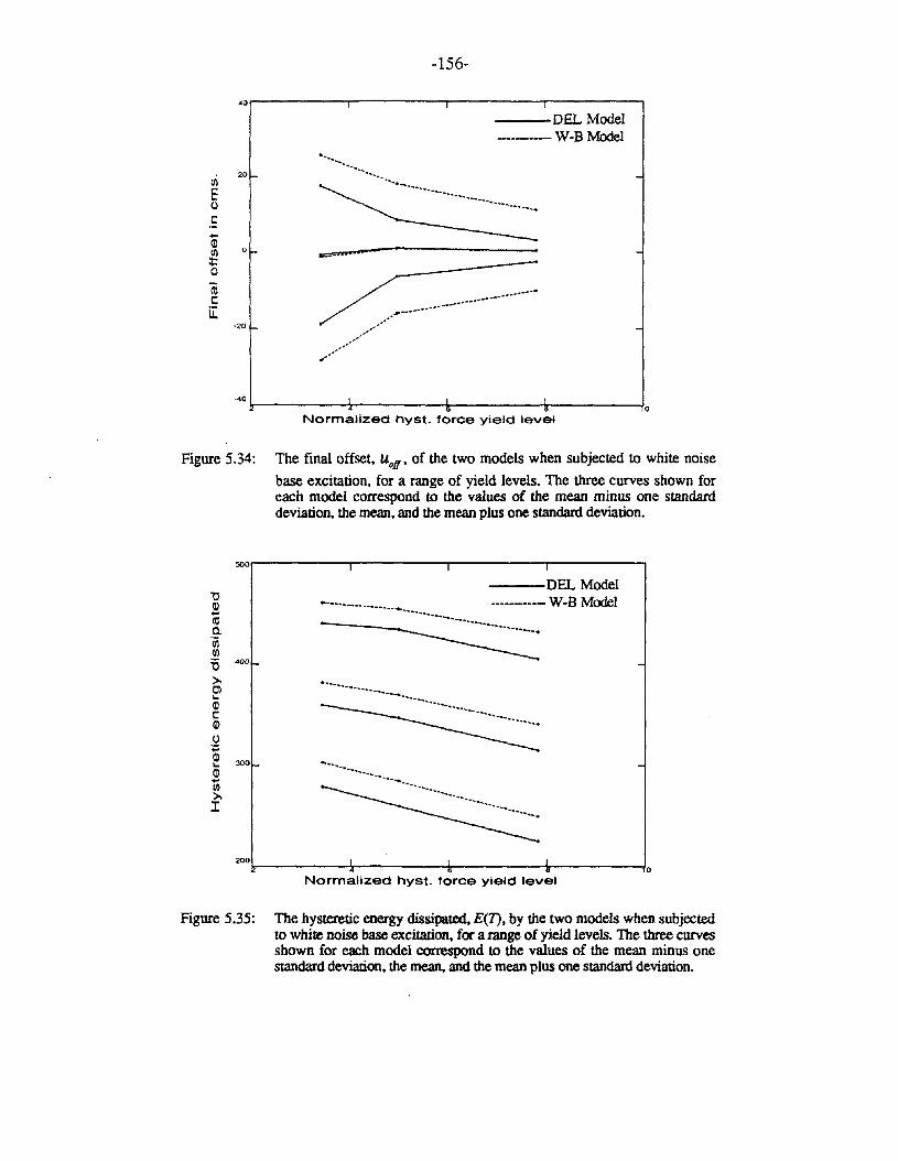
-156-
40,--------..,...------.-------,.-------,---DEL Model--------- W-B Model
IIC="=''"'-'
..,_.., ..., ..._-,..._,....._...".,--
, ......•..............•...........•,,-,,-'.'..-..-
-".... " ..~.
20Ul
Euc..III
0Ul:::0
icu:
-20
-401,-- -+ +- -4. ---10
Normalized hyst. force yield level
Figure 5.34: The final offset. Uoff ' of the two models when subjected to white noise
base excitation, for a range of yield levels. The three curves shown foreach model correspond to the values of the mean minus one standarddeviation, the mean, and the mean plus one standard deviation.
500,--------..,...------.------..,.-----...,
•....-._-..-"'."-.-" -...."-" -"" ""-.-........•
.., .." ,._.,.,_ ".,.." ..
---DEL Model.------....._..._._.__.._.__.._..__._....~~~.~~=~~~~ W-B Model'tlQ)..eu0.'iiiUl=0 400
>-ElIIICQ)
U:;:;~ 300Q)..I/J>I
2001,- -+ +- -4.,...- ---10
Normalized hyst. force yield level
Figure 5.35: The hysteretic energy dissipated, E(1), by the two models when subjectedto white noise base excitation, for a range of yield levels. The three curvesshown for each model correspond to the values of the mean minus onestandard deviation. the mean. and the mean plus one standard deviation.
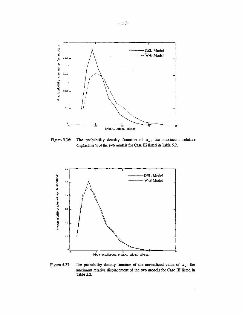
-157-
0.05 r------.-----.-----........-------,---DEL Model'--WeB Model
,
............",
'"..............................-
0).;-----~,------,b,---..::::::==·::;j:··.,;.·..;;;;;··;;;·-::;,·-=-~,00
).01
co:;:tlC::l 0.04....
:0t'iI 0.02.co...Il.
Max. abs. disp.
Figure 5.36: The probability density function of u",. the maximum relativedisplacement of the two models for Case ill listed in Table 5.2.
0.6r------.-----.-----........-------,
>-..iiicQ)'0>-:E:0lU.co..a.
0.5
0.4
0.3
0.2
0.1
---DEL Model----- W-B Model
0l.- -J,.. .J.-__-=~~----___l.
Normalized max. abs. disp.
Figure 5.37: The probability density function of the normalized value of u"'. themaximum relative displacement of the two models for Case ill listed inTable 5.2.
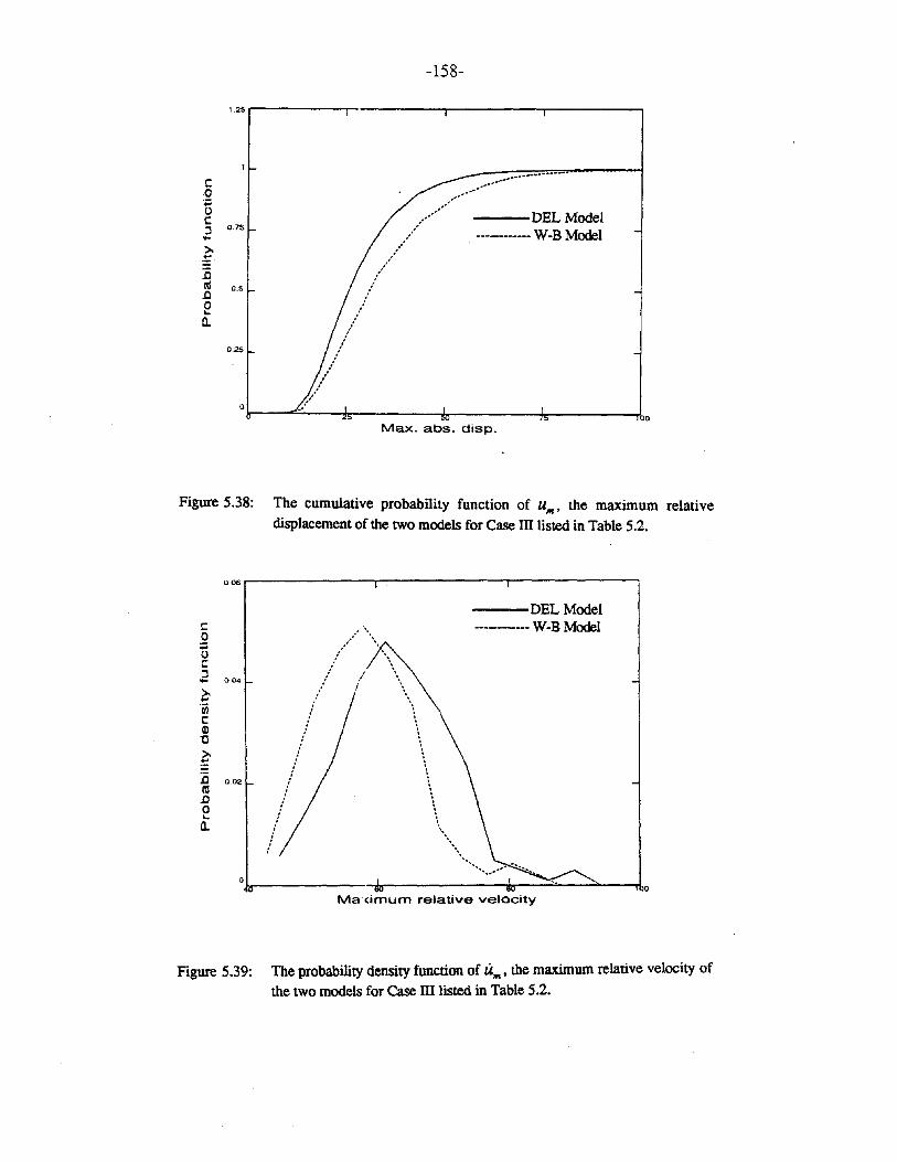
-158-
1.2$,-------r--------.------~----____,
.......................•..........
...../ DEL Model.... ----- WeB Model
/**..",..
/'/I
..-.."""
°r--:;.··--~-----~--------.j~----......l,o
c0;0C:::l 0.75....>..t: .
:cell 0.5.00~
!l.
0.25
Max. abs. disp.
Figure 5.38: The cumulative probability function of U",. the maximum relativedisplacement of the two models for Case ill listed in Table 5.2.
0],,- _
---DEL Model--W-BModel
...···.·····
'........................ ...........
.II
006
C0;0C:::l
004....>....'iiicQl'0>.:!::
:c 002ell.00...!l.
Ma'(imum relative velocity
Figure 5.39: The probability density function of U".. the maximum relative velocity ofthe two models for Case ill listed in Table 5.2.
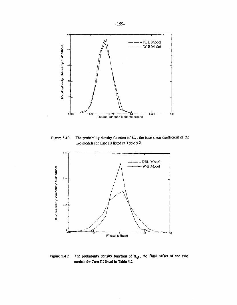
-159-
so,------r------,,..-------r-------.------,
co 40.;:;oC:J->-.. 30·wCQl"0>-.~ 20
:0CIl.Qo...a. '0
---DEL Model------- W-B Model
l3ase shear coeffecient
Figure 5.40: The probability density function of Cb , the base shear coefficient of the
two models for Case III listed in Table 5.2.
0.03r------,------,-------..-------.
co;:;(JC:l-
:iseu.co...a.
0.02
0.01
---DEL Model----W-B Model
Final offset
Figure 5.41: The probability density function of uoff ' the final offset of the two
models for Case III listed in Table 5.2.
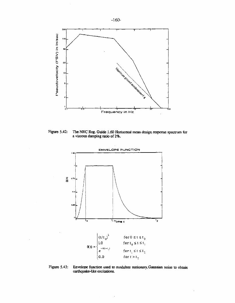
-160-
200
()Q)
100m"-c:c: 50
)'(f)a.
20"">.%'-'--,....
'0'4-~~%-"' __',0 10
Q)> d'",O "-0 ~Q. -'--'0 5 O'",C -'"
:l ""1> "'--,Q)~~. '--m
o.,~ """a.2 d' '
1
O. 00
Frequency in Hz
Figure 5.42: The NRC Reg. Guide 1.60 Horizontal mean design response spectrum fora viscous damping ratio of 2%.
ENVELOPE FUNCTION,:zs..---------------------,
- O.7S
as
0.'
10 I, Time t 12
2forO~t~to(tl to)
1.0 forto~t~tl
EXt) = -y(t-t )e 1 fortl~r~r2
0.0 fort>t,,
Figure 5.43: Envelope function used to modulate stationary,Gaussian noise to obtaineanhquake-like excitations.
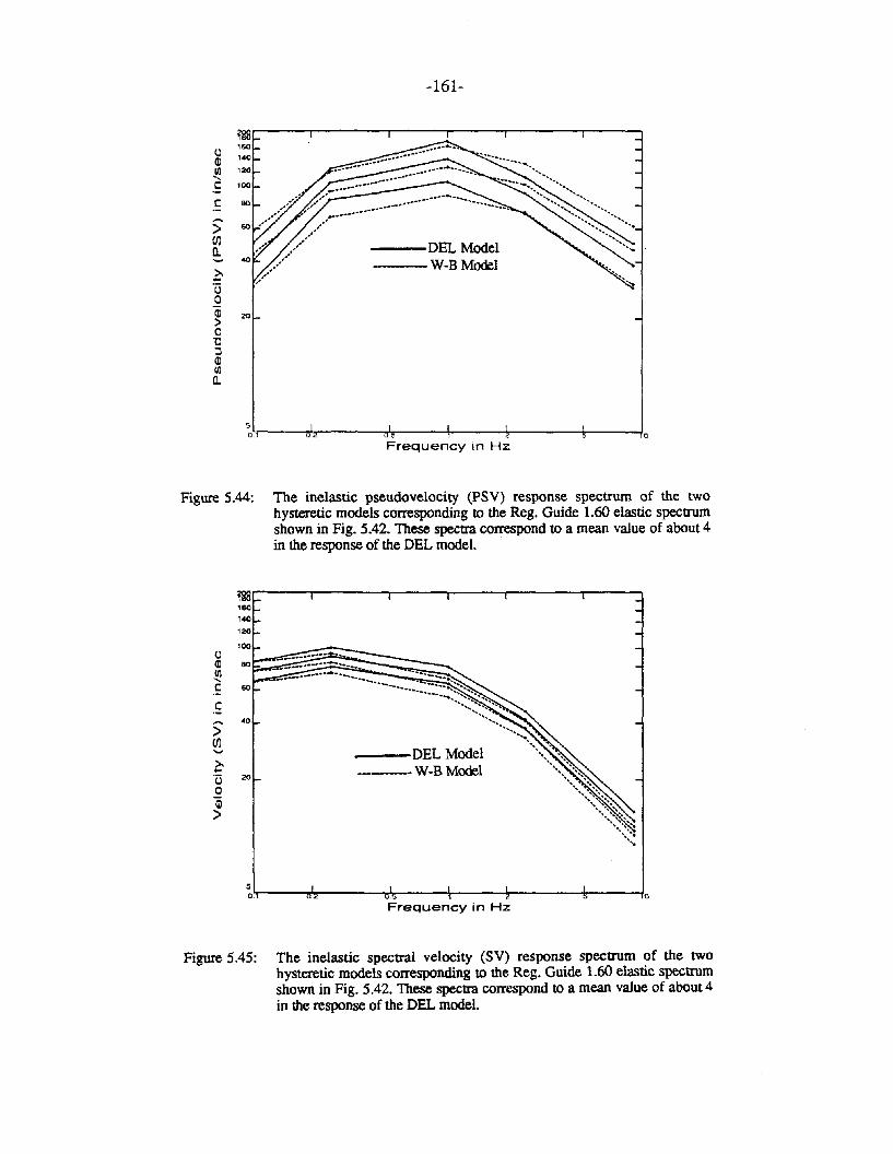
-161-
................................
.. . ..................., .
•.......... "." DEL Model
..,/ W-BModel.'...
20
~'Uoi>o'C~
Ql(J)
Cl.
mr-----,r----,.----,-----r------r----.
u ~:Q)Ul"-C
C
>(J)Q.
5oT.----ur----n:----+----+----+----Jo
Frequency in Hz
Figure 5.44: The inelastic pseudovelocity (PSV) response spectrum of the twohysteretic models corresponding to the Reg, Guide 1.60 elastic spectrumshown in Fig. 5.42. These spectra correspond to a mean value of about 4in the response of the DEL model.
uQl~cc,... .0
>(J)
),....'u 20
oi>
---DEL Model,--- W-B Model
~'r.----uT---~:__--+---_lr----...j,----JoFrequency in Hz
Figure 5.45: The inelastic spectral velocity (SV) response spectrum of the twohysteretic models corresponding to the Reg. Guide 1.60 elastic spectrumshown in Fig. 5.42. These spectra correspond to a mean value of about 4in the response of the DEL model.
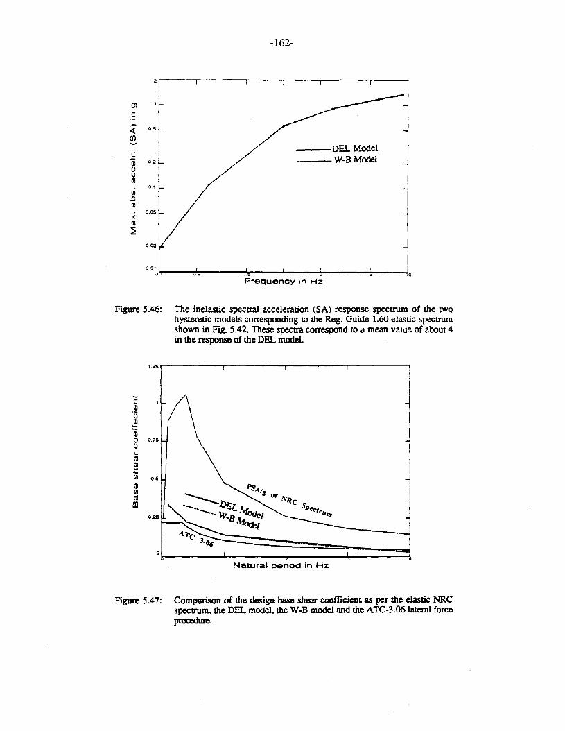
-162-
2 ,...-----...,.----,----....-------.-----..,.---.....,
Clc:-.< 0.5
rJ)......
DEL Modelc:Qi 02 W-BModel(J(Jell
0'In!lal
O.OSxell~
0.02
00. !r----rr.r-----"J...---4---4_----~--....joFrequency in Hz
Figure 5.46: The inelastic specual acceleration (SA) response spectrum of the twohysteretic models corresponding to the Reg. Guide 1.60 elastic spectrumshown in Fig. 5.42. These spectra correspond f(\ cl mean vahle of about 4in the response of the DEL model
1.25
..c:Q)'0Q)......Q)0 0.75(J...ellQ).c:Ul 0.5
Q)Ulell
CD0.25
0J,------\O-----4-----.....<.....------!Natural period in Hz
Figure 5.47: Comparison of the design base shear coefficient as per the elastic NRCspectrum. the DEL model, the W-B model and the ATC-3.06lateral forceprocedure.
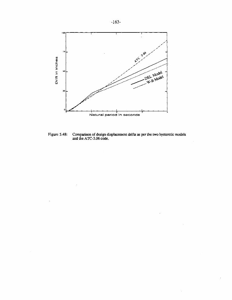
-163-
l00,------r------r------.,....--------,
75
tilQ).s:()cC
50
......";:Q
25
°1r-"~----_+__-----_I,_-----_I,_----___!,4
Natural period in seconds
Figure 5.48: Comparison of design displacement drifts as per the two hysteretic modelsand the ATC-3.06 code.
-164-
CHAPTER 6
SUMMARY· AND CONCLUSIONS
Based on the fIrst fIve chapters of this thesis, a concluding summary on the analysis
carried out and the results obtained may be presented as follows:
(1) Recently proposed mathematical representations for certain piecewise-linear hysteretic
models have been benefIcial in the sense that they have helped cast the models in a
history-independent framework, thus enabling a stochastic linearization to determine the
approximate response statistics. Such representations are available for the elastoplastic
and bilinear models, the polylinear model, the double-bilinear model, the Clough
Johnston model, the slip model, the origin-oriented model, the peak-oriented model,
etc. Unfortunately, there are no curvilinear hysteretic models for which these
representations are currently available; as a matter of fact, it is not clear whether such
representations involving only a small number of additional state variables exist at all
for curvilinear models.
(2) When subjected to transient loading, the models belonging to the Distributed Element
class of curvilinear hysteretic models satisfy an extended version of the Massing's
hypothesis [24], which was originally proposed by Massing for steady-state behavior.
This fact does not help in the equivalent linearization of the hysteretic models.
However, it does simplify signifIcantly the numerical implementation of the models
when they are used to describe the hysteretic behavior of a system subjected to an
arbitrary transient loading. This simplifIcation, combined with the ability of these
models to reproduce a wide range of hysteretic behavior, including both degrading and
nondegrading systems, makes the Distributed Element class of models an excellent
choice for the mathematical modeling of physical systems.
-165-
(3) A relatively simple identification procedure for nonlinear systems has been proposed in
Chapter 3, which is based on matching the slopes of the hysteretic branches of the
restoring force diagram rather than on the time history of the response. This procedure
can be applied to hysteretic as well as to nonhysteretic systems. Examples shown in the
same chapter indicate that the method is satisfactory for systems whose hysteretic
behavior is governed by the bilinear model or by the endochronic model, for instance,
the Wen-Bouc model.
(4) The response behavior of endochronic models, such as that of the Wen-Bouc model
examined in Chapters 4 and 5, raises serious questions about the applicability of these
models to represent physical hysteretic structures. The Wen-Bouc model, when
subjected to certain quasi-static loading sequences, exhibits some inconsistent response
behavior, for instance, displacement drift, loop nonclosure, stiffening, force relaxation
to a zero mean value, etc. Also, these models violate the Drucker's and Ilyushin's
stability postulates, calling to attention the possibility of inaccurate numerical solutions
andlor nonunique solutions.
The instability of the endochronic models becomes quite apparent in Chapter 5
when the Wen-Bouc model is used to model a structure exhibiting the P-o
phenomenon. In this case, a suddenly applied external load on a structure causes very
large response deformations, leading to its eventual collapse. This tendency to predict
unusually large displacements is especially pronounced for very small values of the
post-yielding system stiffness, andlor when the external load has a nonzero mean
value. The possibility of the spurious instability predictions by these models raises the
concern that it may not be possible to determine whether a failure predicted during
analysis is due to the mathematical modeling, or to the actual failure of the structure to
withstand excessive loading.
-166-
It may be recalled that one of the most prominent 'applications of the endochronic
models has been in the estimation of the approximate response statistics of hysteretic
systems subjected to stochastic excitation. With this in mind, a simulation analysis was
performed with the Wen-Bouc model and the physically based Distributed Element
model with identical initial loading behavior, in order to evaluate the ability of the
endochronic model to predict satisfactorily the stochastic response of physical systems.
The difference in the response statistics of the two models varies widely depending on
the response quantity being extracted and the type of system (value of post-yielding
stiffness, number of degrees of freedom, etc.). In one case with nonzero mean, white
noise base excitation, the mean of the absolute value of the response displacement
predicted by the W-B model is about 1.72 times the corresponding value provided by
the Distributed Element model. In this context, a remark needs to be made. Generally
speaking, it is observed that velocity predictions by the Wen-Boue model are better than
displacement and displacement-related quantities like ductility and final offset. By the
same token, estimates of the acceleration-related quantities like the base shear
coefficient seem to be even better than those of the velocity.
In view of the observed differences in the predicted values of certain response
quantities in the simulation analysis, the following observation may be made. Even
though the mathematical structure of the endochronic models is quite elegant and rather
readily affords a direct stochastic linearization, it is a moot point as to how relevant the
approximate response statistics obtained by the use of such models are in the analysis
of physical hysteretic systems, because, simply put, these models are capable of
behaving in a fashion quite inconsistent with realistic structural behavior. Caution must
therefore be exercised in interpreting the estimates of response statistics obtained with
the use of these models in the description of hysteretic behavior of nonlinear systems.
-167-
In light of the above conclusions, a few suggestions for continued research in the
analysis of hysteretic structures may be made here. There are basically two broad avenues
where further study would be profitabie. The first is in improved mathematical modeling of
hysteretic systems. An ideal mathematical model should satisfy the following properties:
(a) the model should be able to capture most of the important attributes of the response
behavior of physical systems,
(b) the model should not exhibit abnormal characteristics that are not usually observed in
physical systems, and
(c) the model representation should be simple enough to readily facilitate deterministic and
stochastic analysis, including linearization.
It is clear that the piecewise-linear models satisfy (b) and (c) but not (a), the endochronic
models satisfies (a) and (c) but not (b), and the Distributed Element models satisfy (a) and
(b) but not (c), since they cannot be easily linearized in order to obtain approximate
response statistics. Whether or not a model satisfying (a), (b) and (c) exists remains to be
seen.
One possible model for hysteresis, containing some features of both the endochronic
and the Distributed Element models, may be proposed as follows. It may be recalled that in
the case of the endochronic models, the slopes of the restoring force diagram depend only
on the instantaneous value of the restoring force, while in the case of the Distributed
Element models, they depend not only on the instantaneous value of the restoring force, but
also on all of the nested turning points. As in the case of the bounding·surface model
proposed by Dafalias [16], the slopes of the restoring force diagram for the suggested
model depend only on the most recent turning point in addition to the usual dependence on
the instantaneous value of the restoring force. The slope of any loading/reloading
/unloading path is assumed to vary linearly from the value of the initial system stiffness at
the point of load reversal to an asymptotic value of zero at the maximum or yielding value
-168-
of the force. By its very formulation, the hysteresis loops are guaranteed to close at least
partially. The hysteretic behavior of this model is similar to that reported by Jennings in
[25].
In the search for improved mathematical models, one interesting field of investigation
may lie in the possibility of extending the Massing's hypothesis to two and three
dimensions. Iwan [21] has extended the hysteretic restoring force behavior of the one
dimensional class of Distributed Element models to three dimensions by introducing the
concept of nested yield surfaces. It will be instructive to determine whether the Massing's
hypothesis can in some way be extended to this three-dimensional class of models.
The second area of considerable research potential is in the possible generalization of
the theory of equivalent linearization so as to include the class of Distributed Element
models. For this purpose, it may be helpful to start with the history-independent
representation for the parallel-series model indicated by Eqn. (2.42). Investigations may
also be undertaken to examine the feasibility of linearizing the Dafalias-like model
suggested earlier.
It is evident that the modeling and analysis of hysteretic systems is an area of
immense research potential and challenge. Every effort must be made to facilitate clear
understanding of the hysteretic nature of nonlinear response behavior, considering its
crucial importance in structural dynamics.
-169-
REFERENCES
[1] American Standards Institute, New York, "American National Standards
and Building Code Requirements For Minimum Design Loads in Buildings and Other
Structl}Ies," ANSI A 58.1-1972.
[2] Applied Technology Council, "Tentative Provisions for the Development of
Seismic Regulations for Buildings (Including Proposed Amendments)," ATC 3-06
(Amended), Second printing, April 1984.
[3] Asano, K. and Iwan, W.D., "An Alternative Approach to The Random Response
of Bilinear Hysteretic Systems," Earthquake Engineering and Structural Dynamics,
Vol. 12,229-236, 1984.
[4] Atalik, T.S. and Utku, S., "Stochastic Linearization of Multi Degree-Of
Freedom Nonlinear Systems," Earthquake Engineering and Structural Dynamics,
VolA, 411-420, 1974.
[5] Baber, T.T., "Nonzero Mean Random Vibration of Hysteretic Systems," Journal
ofApplied Mechanics, Vol. 110, No.3, 1036-1049, 1984.
[6] Bardet, J.P, "Application of Plasticity Theory to Soil Behavior: A New Sand
Model," Ph. D. Dissertation, California Institute of Technology, Pasadena, 1983.
[7] Bazant, Z.P. and Bhat, P., "Endochronic Theory of Inelasticity and Failure of
Concrete," Journal of the Engineering Mechanics Division, ASCE, Vol. 12, No.
EM4, 701-722, August 1976.
[8] Beck, J.L, "Determining Models of Structures from Earthquake Records," Ph. D
Dissertation, California Institute of Technology, Pasadena, 1978.
[9] Bycroft, G.N., "White Noise Representation of Earthquakes," Journal of the
Engineering Mechanics Division, Transactions of the ASCE, Vol. 86, No. EM2, 1
16, April 1960.
[10] Casciyati, "Nonlinear Stochastic Dynamics of Large Structural Systems By
Equivalent Linearization," Proceedings of the ICASPS, the Fifth International
Conference on Application of Statistics and Probability in Soil and Structural
Engineering, University of British Columbia, Vancouver, 1987.
[11] Caughey, T.K., "Random Excitation of a System with Bilinear Hysteresis,"
Journal ofApplied Mechanics, ASME, Vol. 27,649-652, December 1960.
-170-
[12] Caughey, T.K., "Equivalent Linearization Techniques," Journal of Acoustical
Society ofAmerica, Vol. 35, 1706-1711, 1963.
[13] Cifuentes, A.O., "System Identification of Hysteretic Systems," Ph. D.
Dissertation, California Institute 'of Technology, Pasadena, 1984.
[14] Clough, W. and Johnston, S.B., "Effects of Stiffness Degradation on
Earthquake Ductility Requirements," Proceedings of the Second Japan Earthquake
Engineering Symposium, Tokyo, 227-232, October 1966.
[15] Clough, R.W. and Penzien, J., Dynamics Of Structures, McGraw-Hill
Publications: New York, 1975.
[16] Dafalias, Y., "On Cyclic and Anisotropic Plasticity," Ph. D. Dissertation in
Engineering Science, University of California, Berkeley, 1975.
[17] Hildebrand, F.B., Introduction to Numerical Analysis, Dover Publications: New
York, pp. 290-292, 1974.
[18] Housner, G.W., "Characteristics of Strong-Motion Earthquakes," Bulletin of the
Seismological Society ofAmerica, Vol. 37, 19-31, 1947.
[19] Iemura, H. and Jennings, P.C., "Hysteretic Response of a Nine-Story
Reinforced Concrete Building," International Journal ofEarthquake Engineering and
Structural Dynamics, Vol. 3, 183-201, 1974.
[20] Iwan, W.D., " A Distributed-Element Model for Hysteresis and its Steady-State
Dynamic Response," Journal of Applied Mechanics, ASME, Vol. 33, No.4, 893
900, 1966.
[21] Iwan, W.D., "On a Class of Models for the Yielding Behavior of Continuous And
Composite Systems," Journal of Applied Mechanics, ASME, Vol. 34, No.3, 612
617, 1967.
[22] Iwan, W.D., "A Generalization of the Concept of Equivalent Linearization,"
International Journal ofNonlinear Mechanics, Vol. 8,279-287, 1973.
[23] Iwan, W.D., "Estimating Inelastic Response Spectra from Elastic Spectra,"
Earthquake Engineering and Structural Dynamics, Vol. 8, 375-388, 1980.
[24] Jayakumar, P., "Modeling and Identification in Structural Dynamics," Ph. D.
Dissertation, California Institute of Technology, Pasadena, 1987.
[25] Jennings, P.C., "Response of Simple Yielding Structures to Earthquake
Excitation," Ph. D. Dissertation, California Institute of Technology, Pasadena, 1963.
[26] Jennings, P.C., Housner, G.W. and Tsai, N.C., "Simulated Earthquake
Motions," Earthquake Engineering Research Laboratory Report, California Institute
of Technology, Pasadena, 1968.
-171-
[27] Jeong, G.D., "Cumulative Damage of Structures Subjected to Response Spectrum
Consistent Random Processes," Ph. D. Dissertation, California Institute of
Technology, Pasadena, 1985.
[28] Masing, G., "Eigenspannungen·Und Verfestigung Beim Messing," Proceedings of
the Second International Congressfor Applied Mechanics, Zurich, Switzerland, 332
335, 1926 (in German).
[29] Mason, A.B., Jr., "Some Observations on the Random Response of Linear and
Nonlinear Dynamical Systems," Ph. D. Dissertation, California Institute of
Technology, Pasadena, 1979.
[30] Mason, A.B., Jr., and Iwan, W.D., "An Approach to the First Passage
Problem in Random Vibration," Journal of Applied Mechanics, Vol. 50, 641-646,
September 1983.
[31] Masri, S.F. and Caughey, T.K., "A Nonparametric Identification Technique
for Nonlinear Dynamic Problems," Journal ofApplied Mechanics, Vol. 46, 433-447,
June 1979.
[32] McVerry, G.H., "Frequency Domain Identification of Structural Models from
Earthquake Records," Ph. D. Dissertation, California Institute of Technology,
Pasadena, 1979.
[33] Morrow, J. and Sinclair G., "Cyclic Stress Relaxation," ASTM Symposium on
Basic Mechanics of Fatigue, ASTM, Special Technical Publication 237, Boston,
1958.
[34] Nuclear Regulatory Commission, "Design Response Spectra for Seismic
Design," Reg. Guide 1.60, Revision 1, December 1973.
[35] OZdemir, H., "Nonlinear Transient Dynamic Analysis of Yielding Structures," Ph.
D. Dissertation, University of California, Berkeley, June 1976.
[36] Paparizos, L.G., "Some Observations on the Random Response of Hysteretic
Systems," Ph. D. Dissertation, California Institute of Technology, Pasadena, 1986.
[37] Park, Y.J., Wen, Y.K. and Ang, A. H-S, "Random Vibration of Hysteretic
Systems under Bi-directional Ground Motions," Earthquake Engineering and
Structural Dynamics, Vol. 14,543-557, 1986.
[38] Picard, E., "La Mecanique Classique et Ses Approximations Successive," Revista
di Scienza, Vol. 1,4-15, 1907 (In French).
[39] Popov, E.P., "Seismic Behavior of Structural Assemblages," Journal of the
Structural Division, Proceedings of the ASCE, Vol. 106, 1451-1474, July 1980.
-172-
[40] Rice, J.R., "On the Structure of Stress-Strain Relations for Time-Dependent Plastic
Deformation in Metals," Journal ofApplied Mechanics, Vol. 37, 728-737, 1970.
[41] Rice, J.R., "Continuum Mechanics and Thermodynamics of Plasticity in Relation
to Microscale Deformation Mechanisms," Constitutive equations in Plasticity, pp. 23
79, MIT Press, Cambridge, Mas.sachusetts.
[42] Rosenblueth, E. and Bustamente, J.E., "Distribution of Structural Response
to Earthquakes," Journal ofthe Engineering Mechanics Division, No. EM3, 75-106,
June 1962.
[43] Salmon, C.G. and Johnson, J.E., Steel Structures - Design And Behavior,
Second Edition, Harper and Row: New York, 1980.
[44] Sandler, I.S., "On the Uniqueness and Stability of Endochronic Theories Of
Material Behavior," Journal ofApplied Mechanics, Vol. 45, 263-266, 1978.
[45] Spanos, P.D. and Iwan, W.D., "On the Existence and Uniqueness of Solutions
Generated by Equivalent Linearization," International Journal of Nonlinear
Mechanics, VoL 13, 71-78, 1978.
[46] Sues, R.H., Wen, Y.K. and Ang, A. H-S., "Stochastic Seismic Performance
Evaluation of Buildings," Civil Engineering Studies, Structural Series No. 506,
University of Illinois at Urbana-Champaign, Urbana, Illinois, May 1973; also,
Journal ofApplied Mechanics, Vol. 114, No.5, 833-846, May 1988.
[47] Suzuki, Y. and Minai, R., " A Method of Seismic Response Analysis of
Hysteretic Structures Based on Stochastic Differential Equations," Proceedings of the
Eighth World Conference in Earthquake Engineering, VoL 4, 459-466, 1984.
[48] Suzuki, Y. and Minai, R., "Seismic Reliability Analysis of Hysteretic Structures
Based on Stochastic Differential Equations," Proceedings of the Fourth ICOSSAR,
Vol. 2, 177-186, 1985.
[49] Takeda, T., Sozen, M.A. and Nielsen, N.N., "Reinforced Concrete
Response to Simulated Earthquakes," Journal ofthe Structural Division, Transactions
of the ASCE, Vol. 96, 2557-2573, December 1970.
[50] Valanis, K.C., "On The Foundations of the Endochronic Theory of
Viscoplasticity," Archiwum Mechaniki Stosowanej, Vol. 27, No. 5-6, 857-868,
1975.
[51] Veletsos, A.S. and Newmark, N.M., "Effects of Inelastic Behavior on the
Response of Simple Systems to Earthquake Motions," Proceedings of the Second
World Conference on Earthquake Engineering, Tokyo, Japan, Vol. 2, 895-912,
1960.
-173-
[52] Volterra, V., Theory of Functionals and Integro-differential Equations, Dover
Publications: New York, 1959.
[53] Wen, Y.K., "Equivalent Linearization for Hysteretic Systems under Random
Excitations," Journal of Applied Mechanics, ASME, Vol. 47, No.1, 150-154,
March 1980.
[54] Wen, Y.K., "Stochastic Response and Damage Analysis of Inelastic Structures,"
Probabilistic Engineering Mechanics, Vol. 1, No.1, 49-57, 1986.
[55] Yang, J.N., "On the Normality and Accuracy of Simulated Random Processes,"
Journal ofSound and Vibration, Vol. 26, 417-428, 1973.

CALIFORNIA INSTITUTE OF TECHNOLOGY
Reports Published
by
Earthquake Engineering Research Laboratory*Dynamic Laboratory
Disaster Research Center
Note: Numbers in parenthesis are Accession Numbers assigned by the NationalTechnical Information Service; these reports may be ordered from the National TechnicalInformation Service, 5285 Port Royal Road, Springfield, Virginia, 22161. AccessionNumbers should be quoted on orders for reports (PB - -). Reports without thisinformation either have not been submitted to NTIS or the information was not availableat the time of printing. An NIA in parenthesis indicates that the report is no longeravailable at Caltech.
1. Alford, J.L., G.W. Hausner and R.R. Martel, "Spectrum Analysis of Strong-MotionEarthquake," 1951. (Revised August 1964). (N/A)
2. Housner, G.W., "Intensity of Ground Motion During Strong Earthquakes," 1952. (N/A)
3. Hudson, D.E., J.L. Alford and G.W. Hausner, "Response of a Structure to an ExplosiveGenerated Ground Shock," 1952. (N/A)
4. Housner, G. W., "Analysis of the Taft Accelerograrrt of the Earthquake of 21 July 1952." (N/ A)
5. Housner, G.W., "A Dislocation Theory of Earthquakes," 1953. (N/A)
6. Caughey, T.K. and D.E. Hudson, "An Electric Analog Type Response Spectrum," 1954.(N/A)
7. Hudson, D.E. and G.W. Housner, "Vibration Tests of a Steel-Frame Building," 1954. (N/A)
8. Housner, G.W., "Earthquake Pressures on Fluid Containers," 1954. (N/A)
9. Hudson, D.E., "The Wilmot Survey Type Strong-Motion Earthquake Recorder," 1958. (N/A)
10. Hudson, D.E. and W.D. Iwan, "The Wilmot Survey Type Strong-Motion EarthquakeRecorder, Part II," 1960. (N/A)
11. Caughey, T.K., D.E. Hudson and RV. Powell, "The CIT Mark II Electric Analog TypeResponse Spectrum Analyzer for Earthquake Excitation Studies," 1960. (N/A)
12. Keightley, W.O., G.W. Housner and D.E. Hudson, "Vibration Tests of the Encino Dam IntakeTower," 1961. (N/A)
* To order directly by phone, the number is (703) 487-4650.
REPORTS page 1
13. Merchant, H.C., "Mode Superposition Methods Applied to Linear Mechanical Systems UnderEarthquake Type Excitation," 1961. (N/A)
14. Iwan, w.n., "The Dynamic Response of Bilinear Hysteretic Systems," 1961. (N/A)
15. Hudson, D.E., "A New Vibration Exciter for Dynamic Test of Full-Scale Structures," 1961. .(N/A)
16. Hudson, D.E., "Synchronized Vibration Generators for Dynamic Tests of Full-ScaleStructures," 1962. (N/A)
17. Jennings, P.C., "Velocity Spectra of the Mexican Earthquakes of 11 May and 19 May 1962,"1962. (N/A)
18. Jennings, P.C., "Response of Simple Yielding Structures to Earthquake Excitation," 1963.(N/A)
19. Keightley, W.O., "Vibration Tests of Structures," 1963. (N/A)
20. Caughey, T.K. and M.E.J. O'Kelly, "General Theory of Vibration of Damped Linear DynamicSystems," 1963. (N/ A)
21. O'Kelly, M.E.J., "Vibration of Viscously Damped Linear Dynamic Systems," 1964. (N/A)
22. Nielsen, N.N., "Dynamic Response of Multistory Buildings," 1964. (N/ A)
23. Tso, W.K., "Dynamics of Thin-Walled Beams of Open Section," 1964. (N/A)
24. Keightley, W.O., "A Dynamic Investigation of Bouquet Canyon Dam," 1964. (N/A)
25. Malhotra, R.K., "Free and Forced Oscillations of a Class of Self-Excited Oscillators," 1964.
26. Hanson, R.D., "Post-Elastic Response of Mild Steel Structures," 1965.
27. Masri, S.F., "Analytical and Experimental Studies of Impact Dampers," 1965.
28. Hanson, R.D., "Static and Dynamic Tests of a Full-Scale Steel-Frame Structures," 1965.
29. Cronin, D.L., "Response of Linear, Viscous Damped Systems to Excitations Having TimeVarying Frequency," 1965.
30. Hu, P.Y.-F., "Analytical and Experimental Studies of Random Vibration," 1965.
31. Crede, C.E., "Research on Failure of Equipment when Subject to Vibration," 1965.
32. Lutes, L.D., "Numerical Response Characteristics of a Uniform Beam Carrying One DiscreteLoad," 1965. (N/A)
33. Rocke, R.D., "Transmission Matrices and Lumped Parameter Models for ContinuousSystems," 1966. (N/ A)
34. Brady, A.G., "Studies of Response to Earthquake Ground Motion," 1966. (N/A)
35. Atkinson, J.D., "Spectral Density of First Order Piecewise Linear Systems Excited by WhiteNoise," 1967. (N/A)
REPORTS page 2
36. Dickerson, J.R., "Stability of Parametrically Excited Differential Equations," 1967. (N/A)
37. Giberson, M.F., "The Response of Nonlinear Multi-Story Structures Subjected to EarthquakeExcitation," 1967. (N/A)
38. Hallanger, L.W., "The Dynamic Stability of an Unbalanced Mass Exciter," 1967.
39. Husid, R., "Gravity Effects on the Earthquake Response of Yielding Structures," 1967. (N/ A)
40. Kuroiwa, J.H., "Vibration Test of a Multistory Building," 1967. (N/A)
41. Lutes, L.D., "Stationary Random Response of Bilinear Hysteretic Systems," 1967.
42. Nigam, N.C., "Inelastic Interactions in the Dynamic Response of Structures," 1967.
43. Nigam, N.C. and P.C. Jennings, "Digital Calculation of Response Spectra from Strong-MotionEarthquake Records," 1968.
44. Spencer, R.A., "The Nonlinear Response of Some Multistory Reinforced and PrestressedConcrete Structures Subjected to Earthquake Excitation," 1968. (N/ A)
45. Jennings, P.C., G.W. Housner and N.C. Tsai, "Simulated Earthquake Motions," 1968.
46. "Strong-Motion Instrumental Data on the Borrego Mountain Earthquake of 9 April 1968,"(USGS and EERL Joint Report), 1968.
47. Peters, R.B., "Strong Motion Accelerograph Evaluation," 1969.
48. Heitner, K.L., "A Mathematical Model for Calculation of the Run-Up of Tsunamis," 1969.
49. Trifunac, M.D., "Investigation of Strong Earthquake Ground Motion," 1969. (N/A)
50. Tsai, N.C., "Influence of Local Geology on Earthquake Ground Motion," 1969. (N/A)
51. Trifunac, M.D., "Wind and Microtremor Induced Vibrations of a Twenty-Two Steel FrameBuilding," EERL 70-01, 1970.
52. Yang, I-M., "Stationary Random Response of Multidegree-of-Freedom Systems," DYNL-100,June 1970. (N/A)
53. Patula, E.J., "Equivalent Differential Equations for Non-linear Dynamic Systems," DYNL-101,June 1970.
54. Prelewicz, D.A., "Range of Validity of the Method of Averaging," DYNL-102, 1970.
55. Trifunac, M.D., "On the Statistics and Possible Triggering Mechanism of Earthquakes In
Southern California," EERL 70-03, July 1970.
56. Heitner, K.L., "Additional Investigations on a Mathematical Model for Calculation of Run-Upof Tsunamis," July 1970.
57. Trifunac, M.D., "Ambient· Vibration Tests of a Thirty-Nine Story Steel Frame Building,"EERL 70-02, July 1970.
58. Trifunac, M.D. and D.E. Hudson, "Laboratory Evaluations and Instrument Corrections ofStrong.Motion Accelerographs," EERL 70-04, August 1970. (N/A)
REPORTS page 3
59. Trifunac, M.D., "Response Envelope Spectrum and Interpretation of Strong EarthquakeGround Motion," EERL 70-06, August 1970.
60. Keightley, W.O., "A Strong-Motion Accelerograph Array with Telephone Line Interconnections," EERL 70-05, September 1970.
61. Trifunac, M.D., "Low Frequency Digitization Errors and a New Method for Zero BaselineCorrection of Strong-Motion Accelerograms," EERL 70-07, September 1970.
62. Vijayaraghavan, A., "Free and Forced Oscillations in a Class of Piecewise-Linear DynamicSystems," DYNL-103, January 1971.
63. Jennings, P.C., R.B. Mathiesen and J.B. Hoerner, "Forced Vibrations of a 22-Story SteelFrame Building," EERL 71-01, February 1971. (N/A) (PB 205 161)
64. Jennings, P.C., "Engineering Features of the San Fernando Earthquake of February 9, 1971,"EERL 71-02, June 1971. (PB 202 550)
65. Bielak, J., "Earthquake Response of Building-Foundation Systems," EERL 71-04, June 1971.(N/A) (PB 205 305)
66. Adu, R.A., "Response and Failure of Structures Under Stationary Random Excitation," EERL71-03, June 1971. (N/ A) (PB 205 304)
61. Skattum, K.S., "Dynamic Analysis of Coupled Shear Walls and Sandwich Beams," EERL71-06, June 1971. (N/A) (PB 205 267)
68. Hoerner, J.B., "Model Coupling and Earthquake Response of Tall Buildings," EERL 71-07,June 1971. (N/A) (PB 207635)
69. Stahl, K.J., "Dynamic Response of Circular Plates Subjected to Moving Massive Loads,"DYNL.104, June 1971. (N/A)
70. Trifunac, M.D., F .E. Udwadia and A.G. Brady, "High Frequency Errors and InstrumentCorrections of Strong-Motion Accelerograms," EERL 71-05, 1971. (PB 205 369)
71. Furuike, D.M., "Dynamic Response of Hysteretic Systems With Application to a SystemContaining Limited Slip," DYNL-105, September 1971. (N/A)
72. Hudson, D.E. (Editor), "Strong-Motion Instrumental Data. on the San Fernando Earthquakeof February 9, 1971," (Seismological Field Survey, NOAA, C.LT. Joint Report), September1911. (PB 204 198)
73. Jennings, P.C. and J. Bielak, "Dynamics of Building-Soil Interaction," EERL 72-01, April1912. (PB 209 666)
74. Kim, B.-K., "Piecewise Linear Dynamic Systems with Time Delays," DYNL-106, April 1912.
75. Viano, D.C., "Wave Propagation in a Symmetrically Layered Elastic Plate," DYNL-107, May1972.
76. Whitney, A.W., "On Insurance Settlements Incident to the 1906 San Francisco Fire," DRC72-01, August 1972. (PB 213 256)
REPORTS page 4
77. Udwadia, F.E., "Investigation of Earthquake and Microtremor Ground Motions," EERL 72-02,September 1972. (PB 212 853) .
78. Wood, J .H., "Analysis of the Earthquake Response of a Nine-Story Steel Frame BuildingDuring the San Fernando Earthquake," EERL 72-04, October 1972. (PB 215 823)
79. Jennings, P.C., "Rapid Calculation of Selected Fourier Spectrum Ordinates," EERL 72-05,November 1972.
80. "Research Papers Submitted to Fifth World Conference on Earthquake Engineering, Rome,Italy, 25-29 June 1973," EERL 73-02, March 1973. (PB 220431)
81. Udwadia, F .E. and M.D. Trifunac, "The Fourier Transform, Response Spectra and TheirRelationship Through the Statistics of Oscillator Response," EERL 73-01, April 1973. (PB220458)
82. Housner, G.W., "Earthquake-Resistant Design of High-Rise Buildings," DRC 73-01, July 1973.(N/A)
83. "Earthquake and Insurance," Earthquake Research Affiliates Conference, 2-3 April, 1973, DRC73-02, July 1973. (PB 223 033)
84. Wood, J.H., "Earthquake-Induced Soil Pressures on Structures," EERL 73-05, August 1973.(N/A)
85. Crouse, C.B., "Engineering Studies of the San Fernando Earthquake," EERL 73-04, March1973. (N/A)
86. Irvine, H.M., "The Veracruz Earthquake of 28 August 1973," EERL 73-06, October 1973.
87. Iemura, H. and P.C. Jennings, "Hysteretic Response of a Nine-Story Reinforced ConcreteBuilding During the San Fernando Earthquake," EERL 73-07, October 1973.
88. Trifunac, M.D. and V. Lee, "Routine Computer Processing of Strong-Motion Accelerograrns,"EERL 73-03, October 1973. (N/ A) (PB 226 047/AS)
89. Moeller, T.L., "The Dynamics of a Spinning Elastic Disk with Massive Load," DYNL 73-01,October 1973.
90. Blevins, R.D., "Flow Induced Vibration of Bluff Structures," DYNL 74-01, February 1974.
91. Irvine, H.M., "Studies in the Statics and Dynamics of Simple Cable Systems," DYNL-108,January 1974.
92. Jephcott, D.K. and D.E. Hudson, "The Performance of Public School Plants During the SanFernando Earthquake," EERL 74-01, September 1974. (PB 240 000/AS)
93. Wong, H.L., "Dynamic Soil-Structure Interaction," EERL 75-01, May 1975. (N/A) (PB 247233/AS)
94. Foutch, D.A., G.W. Housner and P.C. Jennings, "Dynamic Responses of Six MultistoryBuildings During the San Fernando Earthquake," EERL 75-02, October 1975. (PB 248144/AS)
REPORTS page 5
95. Miller, R.K., "The Steady-State Response of Multidegree-of-Freedom Systems with a SpatiallyLocalized Nonlinearity," EERL 75-03, October 1975. (PB 252 459/AS)
96. Abdel-Ghaffar, A.M., "Dynamic Analyses of Suspension Bridge Structures," EERL 76-01,May 1976. (PB 258 744/AS)
97. Foutch, D.A., "A Study of the Vibrational Characteristics of Two Multistory Buildings,"EERL 76-03, September 1976. (PB 260 874/AS)
98. "Strong Motion Earthquake Accelerograms Index Volume," Earthquake Engineering ResearchLaboratory, EERL 76-02, August 1976. (PB 260 929/AS)
99. Spanos, P-T.D., "Linearization Techniques for Non-Linear Dynamical Systems," EERL 76-04,September 1976. (PB 266083/AS)
100. Edwards, D.B., "Time Domain Analysis of Switching Regulators," DYNL 77-01, March 1977.
101. Abdel-Ghaffar, A.M., "Studies of the Effect of Differential Motions of Two Foundations uponthe Response of the Superstructure ofa Bridge," EERL 77-02, January 1977. (PB 271 095/AS)
102. Gates, N.C., "The Earthquake Response of Deteriorating Systems," EERL 77-03, March 1977.(PB 271 090/AS)
103. Daly, W., W. Judd and R. Meade, "Evaluation of Seismicity at U.S. Reservoirs," USCOLD,Committee on Earthquakes, May 1. (PB 270036/AS)
104. Abdel-Ghaffer, A.M. and G.W. Housner, "An Analysis of the Dynamic Characteristics of aSuspension Bridge by Ambient Vibration Measurements," EERL 77-01, January 1977. (PB275063/AS)
105. Housner, G.W. and P.C. Jennings, "Earthquake Design Criteria for Structures," EERL 77-06,November 1977 (PB 276 502/AS)
106. Morrison, P., R. Maley, G. Brady and R. Porcella, "Earthquake Recordings on or Near Dams,"USCOLD, Committee on Earthquakes, November 1977. (PB 285 867/AS)
107. Abdel-Ghaffar, A.M., "Engineering Data and Analyses of the Whittier, California Earthquakeof January 1, 1976," EERL 77-05, November 1977. (PB 283 750/AS)
108. Beck, J.L., "Determining Models of Structures from Earthquake Records," EERL 78-01, June1978 (PB 288 806/AS)
109. Psycharis, 1., "The Salonica (Thessaloniki) Earthquake of June 20, 1978," EERL 78-03,October 1978. (PB 290 120/AS)
110. Abdel-Ghaffar, A.M. and R.F. Scott, "An Investigation of the Dynamic Characteristics of anEarth Dam," EERL 78-02, August 1978. (PB 288 878/AS)
111. Mason, A.B., Jr., "Some Observations on the Random Response of Linear and NonlinearDynamical Systems," EERL 79-01, January 1979. (PB 290 808/AS)
112. HeImberger, D.V. and P.C. Jennings (Organizers), "Strong Ground Motion: N.S.F. SeminarWorkshop/' SL-EERL 79-02, February 1978.
REPORTS page 6
113. Lee, D.M., P.C. Jennings and G.W. Housner, "A Selection of Important Strong MotionEarthquake Records," EERL 80.01, January 1980. (PB 80 169196)
114. McVerry, G.H., "Frequency Domain Identification of Structural Models from EarthquakeRecords," EERL 79-02, October 1979. (PB-8o.I94301)
115. Abdel-Ghaffar A.M., R.F .scott and M.J .Craig, "Full-Scale Experimental Investigation of aModern Earth Dam," EERL 80.02, February 1980. (PB-81-123788)
116. Rutenberg, A., P.C. Jennings and G.W. Housner, "The Response of Veterans Hospital Building41 in the San Fernando Earthquake," EERL 80.03, May 1980. (PB-82-201377)
117. Haroun, M.A., "Dynamic Analyses of Liquid Storage Tanks," EERL 80.04, February 1980.(PB-81-123275)
118. Liu, W.K., "Development of Finite Element Procedures for Fluid-Structure Interaction,"EERL 80.06, August 1980. (PB 184078)
119. Yoder, P.J., "A Strain-Space Plasticity Theory and Numerical Implementation," EERL 80.07,August 1980. (PB-82.201682)
120. Krousgrill, C.M., Jr., "A Linearization Technique for the Dynamic Response of NonlinearContinua," EERL 80.08, September 1980. (PB-82-201823)
121. Cohen, M., "Silent Boundary Methods for Transient Wave Analysis," EERL 80.09, September1980. (PB-82-201831)
122. Hall, S.A., "Vortex-Induced Vibrations of Structures," EERL 81-01, January 1981. (PB-82201849)
123. Psycharis, LN., "Dynamic Behavior of Rocking Structures Allowed to Uplift," EERL 81-02,August 1981. (PB.82.212945)
124. Shih, C.-F., "Failure of Liquid Storage Tanks Due to Earthquake Excitation," EERL 81-04,May 1981. (PB-82.215013)
125. Lin, A.N., "Experimental Observations of the Effect of Foundation Embedment on StructuralResponse," EERL 82-01, May 1982. (PB-84-163252)
126. Botelho, D.L.R., "An Empirical Model for Vortex-Induced Vibrations," EERL 82·02, August1982. (PB-84-161157)
127. Ortiz, L.A., "Dynamic Centrifuge Testing of Cantilever Retaining Walls," SML 82-02, August1982. (PB-84-162312)
128. Iwan, W.D. (Editor) "Proceedings of the U.S. National Workshop on Strong-MotionEarthquake Instrumentation, April 12-14, 1981, Santa Barbara, California," CaliforniaInstitute of Technology, Pasadena, California, 1981.
129. Rashed, A., "Dynamic Analysis of Fluid-Structure Systems, " EERL 82-03, July 1982. (PB84-162916)
130. National Academy Press, "Earthquake Engineering Research-1982."
REPORTS page 7
131. National Academy Press, "Earthquake Engineering Research-1982, Overview andRecommendations."
132. Jain, S.K., "Analytical Models for the Dynamics of Buildings," EERL 83-02, May 1983. (PB84-161009)
133. Huang, M.-J., "Investigation of Local Geology Effects on Strong Earthquake Ground Motions,"EERL 83-03, July 1983. (PB-84-161488)
134. McVerry, G.H. and J .L. Beck, "Structural Identification of JPL Building 180 Using OptimallySynchronized Earthquake Records." EERL 83-01, August 1983. (PB-84-162833)
135. Bardet, J.P., "Application of Plasticity Theory to Soil Behavior: A New Sand Model," SML83-01, September 1983. (PB-84-162304)
136. Wilson, J.C., "Analysis of the Observed Earthquake Response of a Multiple Span Bridge,"EERL 84-01, May 1984. (PB-85-240505/AS)
137. Hushmand, B., "Experimental Studies of Dynamic Response of Foundations," SML 83-02,November 1983. (PB-86-115383/A)
138. Cifuentes, A.O., "System Identification of Hysteretic Structures," EERL 84-04, 1984. (PB240489/AS14)
139. Smith, K.S., "Stochastic Analysis of the Seismic Response of Secondary Systems," EERL85-01, November 1984. (PB-85-240497/ AS)
140. Maragakis, E., "A Model for the Rigid Body Motions of Skew Bridges," EERL 85-02,December 1984. (PB-85-248433/AS)
141. Jeong, G.D., "Cumulative Damage of Structures Subjected to Response Spectrum ConsistentRandom Process," EERL 85-03, January 1985. (PB-86-100807)
142. Chelvakumar, K., "A Simple Strain-Space Plasticity Model for Clays," EERL 85-05, 1985.(PB-87-234308/CC)
143. Pak, R.Y.S., "Dynamic Response of a Partially Embedded Bar Under Transverse Excitations,"EERL 85-04, May 1985. (PB-87-232856/A06)
144. Tan, T.-S., "Two Phase Soil Study: A. Finite Strain Consolidation, B. Centrifuge ScalingConsiderations," SML 85-01, August 1985. (PB-87-232864/CC)
145. Iwan, W.D., M.A. Moser and C.-Y. Peng, "Strong-Motion Earthquake Measurement Using aDigital Accelerograph," EERL 84-02, April 1984.
146. Beck, R.T. and J.L. Beck, "Comparison Between Transfer Function and Modal MinimizationMethods for System Identification," EERL 85-06, November 1985. (PB-87-234688/A04)
147. Jones, N.P., "Flow-Induced Vibration of Long Structures," DYNL 86-01, May 1986. (PB-88106646/A08)
148. Peek, R., "Analysis of Unanchored Liquid Storage Tanks Under Seismic Loads," EERL 86-01,April 1986. (PB-87-232872/A12)
REPORTS page 8
149. Paparizos, L.G., "Some Observations on the Random Response of Hysteretic Systems," EERL86-02. 1986. (PB-88235668/CC)
150. Moser, M.A., "The Response of Stick-Slip Systems to Random Seismic Excitation," EERL86-03, September 1986. (PB-89-194427/AS)
151. Burridge, P.B., "Failure of Slopes," SML 87-01, March 1987. (PB-89-194401/AS)
152. Jayakumar, P., "Modeling and Identification in Structural Dynamics," EERL 87-01, May1987. (PB-89-194146/AS)
153. Dowling, M.J., "Nonlinear Seismic Analysis of Arch Dams," EERL 87-03, September 1987.(PB-89-194443/AS)
154. Duron, Z.H., "Experimental and Finite Element Studies of a Large Arch Dam," EERL 87-02,September 1987. (PB-89-194435/AS)
155. Whirley, R.G., "Random Response of Nonlinear Continuous Systems," EERL 87-04,September 1987. (PB-89-194153/AS)
156. Peng, C.-Y., "Generalized Model Identification of Linear and Nonlinear Dynamic Systems,"EERL 87-05, September 1987. (PB-89-194419/AS)
157. Levine, M.B., J.L. Beck, W.D. Iwan, P.C. Jennings and R. RelIes, "Accelerograms Recordedat Caltech During the Whittier Narrows Earthquakes of October 1 and 4, 1987: A PreliminaryReport," EERL 88-01, August 1988. PB-
158. Nowak, P.S., "Effect of Nonuniform Seismic Input on Arch Dams," EERL 88-03, September1988. (PB-89-194450/AS)
159. EI-Aidi, B., "Nonlinear Earthquake Response of Concrete Gravity Dam Systems," EERL 8802, August 1988. (PB-89-193124/AS)
160. Smith, P.W., Jr., "Considerations for the Design of Gas-Lubricated Slider Bearings," DYNL89-01, January 1988. PE-
161. Donlon, W .P., Jr., "Experimental Investigation of the Nonlinear Seismic Response of ConcreteGravity Dams," EERL 89-01, January 1989. PE-
REPORTS page 9