Model Selection and Goodness of Fit

G. Jogesh Babu

Penn State Universityhttp://www.stat.psu.edu/∼babu

Director of Center for Astrostatistics

http://astrostatistics.psu.edu

Astrophysical Inference from astronomical data

Fitting astronomical data

Non-linear regression

Density (shape) estimation

Parametric modeling

Parameter estimation of assumed modelModel selection to evaluate different models

Nested (in quasar spectrum, should one add a broadabsorption line BAL component to a power law continuum).Non-nested (is the quasar emission process a mixture ofblackbodies or a power law?).

Goodness of fit

Chandra Orion Ultradeep Project (COUP)

$4Bn Chandra X-Ray observatory NASA 19991616 Bright Sources. Two weeks of observations in 2003

What is the underlying nature of a stellar spectrum?

Successful model for high signal-to-noise X-ray spectrum.Complicated thermal model with several temperatures

and element abundances (17 parameters)

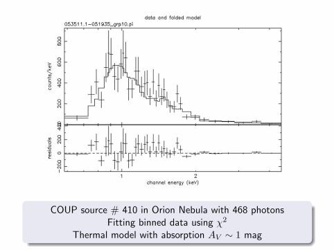
COUP source # 410 in Orion Nebula with 468 photonsFitting binned data using χ2

Thermal model with absorption AV ∼ 1 mag

Best-fit model: A plausible emission mechanism

Model assuming a single-temperature thermal plasma withsolar abundances of elements. The model has three freeparameters denoted by a vector θ.

plasma temperatureline-of-sight absorptionnormalization

The astrophysical model has been convolved with complicatedfunctions representing the sensitivity of the telescope anddetector.

The model is fitted by minimizing chi-square with an iterativeprocedure.

θ = arg minθχ2(θ) = arg min

θ

N∑i=1

(yi −Mi(θ)

σi

)2

.

Chi-square minimization is a misnomer. It is parameter estimationby weighted least squares.

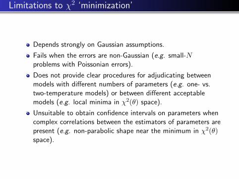
Limitations to χ2 ‘minimization’

Depends strongly on Gaussian assumptions.

Fails when the errors are non-Gaussian (e.g. small-Nproblems with Poissonian errors).

Does not provide clear procedures for adjudicating betweenmodels with different numbers of parameters (e.g. one- vs.two-temperature models) or between different acceptablemodels (e.g. local minima in χ2(θ) space).

Unsuitable to obtain confidence intervals on parameters whencomplex correlations between the estimators of parameters arepresent (e.g. non-parabolic shape near the minimum in χ2(θ)space).

Alternative approach to the model fitting

Fitting to unbinned EDFCorrect model family, incorrect parameter value

Thermal model with absorption set at AV ∼ 10 mag

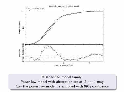
Misspecified model family!Power law model with absorption set at AV ∼ 1 mag

Can the power law model be excluded with 99% confidence

Model Fitting in Astronomy to answer:

Is the underlying nature of an X-ray stellar spectrum anon-thermal power law or a thermal gas with absorption?

Are the fluctuations in the cosmic microwave background bestfit by Big Bang models with dark energy or with quintessence?

Are there interesting correlations among the properties ofobjects in any given class (e.g. the Fundamental Plane ofelliptical galaxies), and what are the optimal analyticalexpressions of such correlations?

Model Selection in Astronomy

Interpreting the spectrum of an accreting black hole such as aquasar. Is it a nonthermal power law, a sum of featurelessblackbodies, and/or a thermal gas with atomic emission andabsorption lines?

Interpreting the radial velocity variations of a large sample ofsolar-like stars. This can lead to discovery of orbiting systemssuch as binary stars and exoplanets, giving insights into starand planet formation.

Interpreting the spatial fluctuations in the cosmic microwavebackground radiation. What are the best fit combinations ofbaryonic, Dark Matter and Dark Energy components? Are BigBang models with quintessence or cosmic strings excluded?

A good model should be

Parsimonious (model simplicity)

Conform fitted model to the data (goodness of fit)

Easily generalizable.

Not under-fit that excludes key variables or effects

Not over-fit that is unnecessarily complex by includingextraneous explanatory variables or effects.

Under-fitting induces bias and over-fitting induces highvariability.

A good model should balance the competing objectives ofconformity to the data and parsimony.

Model Selection Framework

Observed data D

M1, . . . ,Mk are models for D under consideration

Likelihood f(D|θj ;Mj) and loglikelihood`(θj) = log f(D|θj ;Mj) for model Mj .

f(D|θj ;Mj) is the probability density function (in thecontinuous case) or probability mass function (in the discretecase) evaluated at the data D.θi is a pj dimensional parameter vector.

Example

D = (X1, . . . , Xn), Xi, i.i.d. N(µ, σ2) r.v. Likelihood

f(D|µ, σ2) = (2πσ2)−n/2 exp

{− 1

2σ2

n∑i=1

(Xi − µ)2

}

Most of the methodology can be framed as a comparison betweentwo models M1 and M2.

Nested Models

The model M1 is said to be nested in M2, if some coordinates ofθ1 are fixed, i.e. the parameter vector is partitioned as

θ2 = (α, γ) and θ1 = (α, γ0)γ0 is some known fixed constant vector.

Comparison of M1 and M2 can be viewed as a classical hypothesistesting problem of H0 : γ = γ0.

Example

M2 Gaussian with mean µ and variance σ2

M1 Gaussian with mean 0 and variance σ2

The model selection problem here can be framed in terms ofstatistical hypothesis testing H0 : µ = 0, with free parameter σ.

Hypothesis testing for model selection

Hypothesis testing is a criteria used for comparing two models.Classical testing methods are generally used for nested models.

Caution/Objections

M1 and M2 are not treated symmetrically as the nullhypothesis is M1.

Cannot accept H0

Can only reject or fail to reject H0.

Larger samples can detect the discrepancies and more likely tolead to rejection of the null hypothesis.

The “Holy Trinity” of hypotheses tests

H0 : θ = θ0, θ MLE

`(θ) loglikelihood at θ

θ

Loglikelihood

θ0 θ

Wald Test

Based on the (standardized)distance between θ0 and θ

Likelihood Ratio Test

Based on the distance from`(θ0) to `(θ).

Rao Score Test

Based on the gradient ofthe loglikelihood (called thescore function) at θ0.

These three MLE based tests are equivalent to the first order ofasymptotics, but differ in the second order properties.No single test among these is uniformly better than the others.

Wald Test Statistic

Wn = (θn − θ0)2/V ar(θn) ∼ χ2

The standardized distance between θ0 and the MLE θn.

In general V ar(θn) is unknown

V ar(θ) ≈ 1/I(θn), I(θ) is the Fisher’s information

Wald test rejects H0 : θ = θ0 when I(θn)(θn − θ0)2 is large.

Likelihood Ratio Test Statistic

`(θn)− `(θ0)

Rao’s Score (Lagrangian Multiplier) Test Statistic

S(θ0) =1

nI(θ0)

(n∑i=1

f ′(Xi; θ0)f(Xi; θ0)

)2

X1, . . . , Xn are independent random variables with a commonprobability density function f(.; θ).

Example

In the case of data from normal (Gaussian) distribution

f(y; (µ, σ2)) =1√2πσ

exp{− 1

2σ2(y − µ)2

}

S(θ0) =1

nI(θ0)

(n∑i=1

f ′(Xi; θ0)f(Xi; θ0)

)2

Regression Context

y1, . . . , yn data with Gaussian residuals, then the loglikelihood ` is

`(β) = logn∏i=1

1√2πσ

exp{− 1

2σ2(yi − x′iβ)2

}If M1 is nested in M2, then the largest likelihood achievable by M2 will

always be larger than that of M1. Adding a a penalty on larger models

would achieve a balance between over-fitting and under-fitting, leading to

the so called Penalized Likelihood approach.

Information Criteria based model selection – AIC

The traditional maximum likelihood paradigm provides amechanism for estimating the unknown parameters of a modelhaving a specified dimension and structure.

Hirotugu Akaike extended this paradigm in 1973 to the case,where the model dimension is also unknown.

Grounding in the concept of entropy, Akaike proposedan information criterion (AIC), now popularly known asAkaike’s Information Criterion, where both model estimationand selection could be simultaneously accomplished.

AIC for model Mj is 2`(θj)− 2kj . The term 2`(θj) is knownas the goodness of fit term, and 2kj is known as the penalty.

The penalty term increase as the complexity of the modelgrows.

AIC is generally regarded as the first model selection criterion.It continues to be the most widely known and used model selectiontool among practitioners.

Hirotugu Akaike (1927-2009)

Advantages of AIC

Does not require the assumption that one of the candidatemodels is the ”true” or ”correct” model.

All the models are treated symmetrically, unlike hypothesistesting.

Can be used to compare nested as well as non-nested models.

Can also be used to compare models based on differentfamilies of probability distributions.

Disadvantages of AIC

Large data are required especially in complex modelingframeworks.

Not consistent. That is, if p0 is the correct number ofparameters, and k = ki (i = arg maxj 2`(θj)− 2kj), then

limn→∞ P (k > k0) > 0. That is even if we have very largenumber of observations, p does not approach the true value.

Bayesian Information Criterion (BIC)

BIC is also known as the Schwarz Bayesian Criterion2`(θj)− kj log n

BIC is consistent unlike AIC

Like AIC, the models need not be nested to use BIC

AIC penalizes free parameters less strongly than does the BIC

Conditions under which these two criteria are mathematicallyjustified are often ignored in practice.

Some practitioners apply them even in situations where theyshould not be applied.

Caution

Sometimes these criteria are given a minus sign so the goalchanges to finding the minimizer.

Bootstrap for Goodness of Fit

1 Astrophysical Inference from astronomical data

2 Bootstrap for Goodness of Fit

3 Statistics based on EDF

4 Processes with estimated parameters

5 BootstrapParametric bootstrapNonparametric bootstrap

6 Confidence limits under misspecification

Empirical Distribution Function

K-S Confidence bands

F = Fn ±Dn(α)

Statistics based on EDF

Kolmogrov-Smirnov: supx|Fn(x)− F (x)|,

supx

(Fn(x)− F (x))+, supx

(Fn(x)− F (x))−

Cramer-von Mises:

∫(Fn(x)− F (x))2 dF (x)

Anderson - Darling:

∫(Fn(x)− F (x))2

F (x)(1− F (x))dF (x)

These statistics are distribution free if F is continuous &univariate.

No longer distribution free if either F is not univariate orparameters of F are estimated.

Kolmogorov-Smirnov Table

KS probabilities are invalidwhen the model parametersare estimated from thedata. Some astronomers usethem incorrectly.

– Lillifors (1964)

Multivariate Case

Example – Paul B. Simpson (1951)

F (x, y) = ax2y + (1− a)y2x, 0 < x, y < 1

(X1, Y1) ∼ F . F1 denotes the EDF of (X1, Y1)

P (|F1(x, y)− F (x, y)| < .72, for all x, y)

> .065 if a = 0, (F (x, y) = y2x)

< .058 if a = .5, (F (x, y) =12xy(x+ y))

Numerical Recipe’s treatment of a 2-dim KS test is mathematicallyinvalid.

Processes with estimated parameters

{F (.; θ) : θ ∈ Θ} – a family of continuous distributions

Θ is a open region in a p-dimensional space.

X1, . . . , Xn sample from F

Test F = F (.; θ) for some θ = θ0

Kolmogorov-Smirnov, Cramer-von Mises statistics, etc., when θ isestimated from the data, are continuous functionals of theempirical process

Yn(x; θn) =√n(Fn(x)− F (x; θn)

)θn = θn(X1, . . . , Xn) is an estimator θ

Fn – the EDF of X1, . . . , Xn

Bootstrap

Gn is an estimator of F , based X1, . . . , Xn.

X∗1 , . . . , X∗n i.i.d. from Gn

θ∗n = θn(X∗1 , . . . , X∗n)

F (.; θ) is Gaussian with θ = (µ, σ2)

If θn = (Xn, s2n), then

θ∗n = (X∗n, s∗2n )

Parametric bootstrap if Gn = F (.; θn)

X∗1 , . . . , X∗n i.i.d. F (.; θn)

Nonparametric bootstrap if Gn = Fn (EDF)

Parametric bootstrap

X∗1 , . . . , X∗n sample generated from F (.; θn)

In Gaussian case θ∗n = (X∗n, s∗2n ).

Both √n sup

x|Fn(x)− F (x; θn)|

and √n sup

x|F ∗n(x)− F (x; θ∗n)|

have the same limiting distribution

In XSPEC package, the parametric bootstrap is command FAKEIT,which makes Monte Carlo simulation of specified spectral model

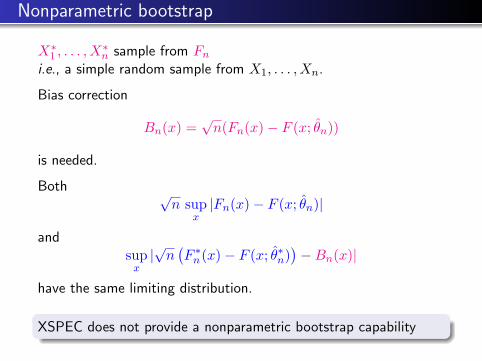
Nonparametric bootstrap

X∗1 , . . . , X∗n sample from Fn

i.e., a simple random sample from X1, . . . , Xn.

Bias correction

Bn(x) =√n(Fn(x)− F (x; θn))

is needed.

Both √n sup

x|Fn(x)− F (x; θn)|

andsupx|√n(F ∗n(x)− F (x; θ∗n)

)−Bn(x)|

have the same limiting distribution.

XSPEC does not provide a nonparametric bootstrap capability

χ2 type statistics – (Babu, 1984, Statistics with linearcombinations of chi-squares as weak limit. Sankhya, Series A, 46,85-93.)

U -statistics – (Arcones and Gine, 1992, On the bootstrap of Uand V statistics. The Ann. of Statist., 20, 655–674.)

Confidence limits under misspecification

X1, . . . , Xn data from unknown H.

H may or may not belong to the family {F (.; θ) : θ ∈ Θ}

H is closest to F (., θ0)

Kullback-Leibler information∫h(x) log

(h(x)/f(x; θ)

)dν(x) ≥ 0∫

| log h(x)|h(x)dν(x) <∞∫h(x) log f(x; θ0)dν(x) = maxθ∈Θ

∫h(x) log f(x; θ)dν(x)

For any 0 < α < 1,

P(√n sup

x|Fn(x)−F (x; θn)− (H(x)−F (x; θ0))| ≤ C∗α

)−α→ 0

C∗α is the α-th quantile of

supx |√n(F ∗n(x)− F (x; θ∗n)

)−√n(Fn(x)− F (x; θn)

)|

This provide an estimate of the distance between the truedistribution and the family of distributions under consideration.

Similar conclusions can be drawn for von Mises-type distances∫ (Fn(x)− F (x; θn)− (H(x)− F (x; θ0))

)2dF (x; θ0),

∫ (Fn(x)− F (x; θn)− (H(x)− F (x; θ0))

)2dF (x; θn).

References

Akaike, H. (1973). Information Theory and an Extension of theMaximum Likelihood Principle. In Second International Symposiumon Information Theory, (B. N. Petrov and F. Csaki, Eds). AkademiaKiado, Budapest, 267-281.

Babu, G. J., and Bose, A. (1988). Bootstrap confidence intervals.Statistics & Probability Letters, 7, 151-160.

Babu, G. J., and Rao, C. R. (1993). Bootstrap methodology. InComputational statistics, Handbook of Statistics 9, C. R. Rao (Ed.),North-Holland, Amsterdam, 627-659.

Babu, G. J., and Rao, C. R. (2003). Confidence limits to thedistance of the true distribution from a misspecified family bybootstrap. J. Statistical Planning and Inference, 115, no. 2, 471-478.

Babu, G. J., and Rao, C. R. (2004). Goodness-of-fit tests whenparameters are estimated. Sankhya, 66, no. 1, 63-74.

Getman, K. V., and 23 others (2005). Chandra Orion UltradeepProject: Observations and source lists. Astrophys. J. Suppl., 160,319-352.