model refrence adaptive control presentation by rishi
DESCRIPTION
ADAPTIVE CONTROLTRANSCRIPT

PRESENTED BY
RISHI KANT SHARMA
ADAPTIVE CONTROL
To adapt means “ to change (oneself) so that one’s behaviour will conform to new or changed circumstances.”
An adaptive controller is a controller with adjustable parameters and a mechanism for adjusting the parameters.
Adaptive control systems have two loops. One loop is a normal feedback loop with the process and the controller. The other loop is the parameter adjustment loop.
A control engineer uses adaptive control because it has useful properties, which can be profitably used to design control system with improved performance and functionality
References: Adaptive control (2nd Edition); Karl Johan Astrom, Bjorn Wittenmark, Prentice Hall

ADAPTIVE CONTROL
PARAMETER ADJUSTMENT
PLANTCONTROLLER
Fig Block diagram of an adaptive system

HISTROY OF ADAPTIVE CONTROL
In early 1950s there was an extensive research on adaptive control in connection with design of autopilots for high performance aircraft. After a significant effort it was found that gain scheduling was a suitable technique for flight control systems.
Model reference adaptive control was suggested by Whitaker etal, to solve the autopilot control problem. The sensitivity method and the MIT rule was used to design the adaptive laws of the various proposed adaptive control schemes. An adaptive pole placement scheme based on the optimal linear quadratic problem was suggested by Kalman
The 1960s State space techniques and stability theory based on Lyapunov were introduced. Developments in dynamic programming, dual control and stochastic control in general, and in system identification and parameter estimation played a crucial role in the reformulation and redesign of adaptive control.
By 1966 Parks and others found a way of redesigning the MIT rule-based adaptive laws used in the MRAC schemes of the 1950s by applying the Lyapunov design approach.
By the mid 1980s, several new redesigns and modifications were proposed and analyzed, leading to a body of work known as robust adaptive control. The focus of adaptive control research in the late 1980s to early 1990s was on performance properties and on extending the results of the 1980s to certain classes of nonlinear plants with unknown parameters.

ADAPTIVE SCHEMES
The different adaptive schemes are as follows: Gain scheduling, Model reference adaptive control (MRAC), Self tuning regulators (STR)& Dual control.
References: Adaptive control (2nd Edition); Karl Johan Astrom, Bjorn Wittenmark, Prentice Hall

GAIN SCHEDULING
In many cases it is possible to find measurable variables that correlate well with changes in process dynamics. These variables can then be used to change the controller parameter. This approach is called gain scheduling as it was used to measure the gain and then change, i.e., schedule, the controller to compensate for changes in the process gain.
Gain scheduling can be viewed as a feedback control system in which the
feedback gains are adjusted by using feedforward compensation.
Fig block diag. for gain scheduling

ADVANTAGES / disadvantages OF GAIN SCHEDULING
ADVANTAGES The advantage of gain scheduling is that the controller gains can be
changed as quickly as the auxiliary measurements respond to parameter Changes. Frequent and rapid changes of the controller gains, however, may lead to instability; therefore, there is a limit as to how often and how fast the controller gains can be changed.
Direct (no complex online calculations are needed). Convenient if relation is known.DISADVANTAGES In gain scheduling, the adjustment mechanism of the controller gains is
precomputed on-line and, therefore, provides no feedback to compensate for incorrect schedules. Unpredictable changes in the plant dynamics may lead to deterioration of performance or even to complete failure.
The high design and implementation costs increase with the number of operating points.
Not always applicable No real learning possibilities
INDIRECT ADAPTIVE CONTROL
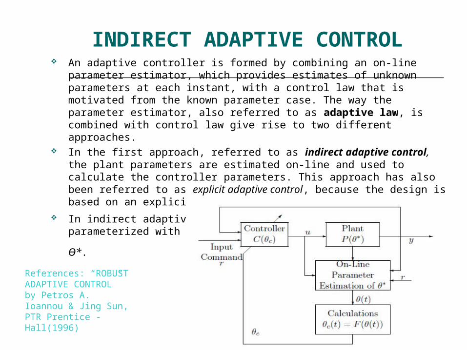
An adaptive controller is formed by combining an on-line parameter estimator, which provides estimates of unknown parameters at each instant, with a control law that is motivated from the known parameter case. The way the parameter estimator, also referred to as adaptive law, is combined with control law give rise to two different approaches.
In the first approach, referred to as indirect adaptive control, the plant parameters are estimated on-line and used to calculate the controller parameters. This approach has also been referred to as explicit adaptive control, because the design is based on an explicit plant model.
In indirect adaptive control, the plant model P(Ɵ*) is parameterized with respect to some
unknown parameter vector Ɵ*.
References: “ROBUST ADAPTIVE CONTROL” by Petros A. Ioannou & Jing Sun, PTR Prentice -Hall(1996)

INDIRECT ADAPTIVE CONTROL
For example, for a linear time invariant (LTI), SISO plant model, Ɵ* may represent the unknown coefficients of the numerator and denominator of the plant model transfer function.
An on-line parameter estimator generates an estimate Ɵ(t) of Ɵ* at each time t by processing the plant input u and output y. The parameter estimate Ɵ(t) specifies an estimated plant model characterized by (Ɵ(t)) that for control design purposes is treated as the “true" plant model and is used to calculate the controller parameter or gain vector Ɵc(t) by solving a certain algebraic equation Ɵc(t) = F(Ɵ(t)) at each time t.
The form of the control law C(Ɵc) and algebraic equation Ɵc = F (Ɵ) is chosen to be the same as that of the control law C(Ɵc*) and equation Ɵc*=F(Ɵ*) that could be used to meet the performance requirements for the plant model P(Ɵ*) if Ɵ* was known. It is, therefore, clear that with this approach, C(Ɵc(t)) is designed at each time t to satisfy the performance requirements for the estimated plant model (Ɵ(t)), which may be different from the unknown plant model P(Ɵ*).
Therefore, the principal problem in indirect adaptive control is to choose the class of control laws C(Ɵc) and the class of parameter estimators that generate Ɵ(t) as well as the algebraic equation Ɵc(t) = F(Ɵ(t)) so that C(Ɵc(t)) meets the performance requirements for the plant model P(Ɵ*) with unknown Ɵ*.
DIRECT ADAPTIVE CONTROL
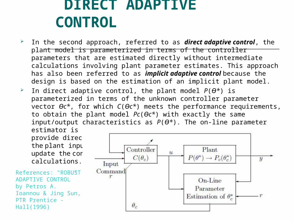
In the second approach, referred to as direct adaptive control, the plant model is parameterized in terms of the controller parameters that are estimated directly without intermediate calculations involving plant parameter estimates. This approach has also been referred to as implicit adaptive control because the design is based on the estimation of an implicit plant model.
In direct adaptive control, the plant model P(Ɵ*) is parameterized in terms of the unknown controller parameter vector Ɵc*, for which C(Ɵc*) meets the performance requirements, to obtain the plant model Pc(Ɵc*) with exactly the same input/output characteristics as P(Ɵ*). The on-line parameter estimator is designed based on Pc(Ɵc*) instead of P(Ɵ*) to provide direct estimates Ɵc(t) of Ɵc* at each time t by processing the plant input u and output y. The estimate Ɵc(t) is then used to update the controller parameter vector Ɵc without intermediate calculations.
References: “ROBUST ADAPTIVE CONTROL” by Petros A. Ioannou & Jing Sun, PTR Prentice -Hall(1996)

SELF TUNING REGULATORS (STR)
In adaptive schemes if the estimates of the process parameters are updated and the controller parameters are obtained from the solution of a design problem using the estimated parameters then it is known as self tuning regulator (STR). The adaptive controller, inner loop consists of the process and the ordinary feedback controller. The parameters of the controller are adjusted by the outer loop, composed of a recursive parameter estimator and a design calculation. If the system is viewed as the automation of process modelling and design, in which the process model and control design are updated at each sampling period, then such type of construction is known as self tuning regulator (STR) to emphasize that the controller automatically tunes its parameter to obtain the desired properties of the closed loop system
References: Adaptive control (2nd Edition); Karl Johan Astrom, Bjorn Wittenmark, Prentice Hall

Dual Control
In this method it is possible to obtain a solution that follows from an abstract problem formulation and uses optimization theory. In dual control approach the uncertainties in the estimated parameters are taken into account in the controller. The controller will also take special action when it has poor knowledge about the process.
A Stochastic Approach
No separation between state variables and modelparametersUncertainties of model parameters are taken into account
Leads to hyperstate T
Estimators generates the conditional probability distribution p(z|y,u)
Minimization of loss function Over control signal u(k)
Dynamic programming
MODEL REFERENCE ADAPTIVE
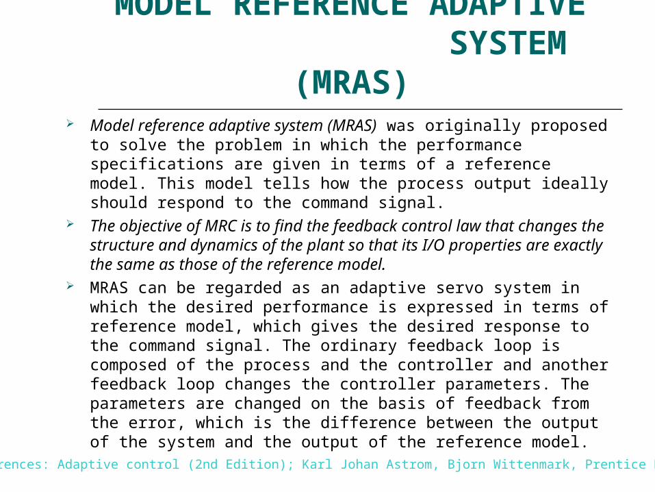
SYSTEM (MRAS) Model reference adaptive system (MRAS) was originally proposed to solve the
problem in which the performance specifications are given in terms of a reference model. This model tells how the process output ideally should respond to the command signal.
The objective of MRC is to find the feedback control law that changes the structure and dynamics of the plant so that its I/O properties are exactly the same as those of the reference model.
MRAS can be regarded as an adaptive servo system in which the desired performance is expressed in terms of reference model, which gives the desired response to the command signal. The ordinary feedback loop is composed of the process and the controller and another feedback loop changes the controller parameters. The parameters are changed on the basis of feedback from the error, which is the difference between the output of the system and the output of the reference model.
References: Adaptive control (2nd Edition); Karl Johan Astrom, Bjorn Wittenmark, Prentice Hall
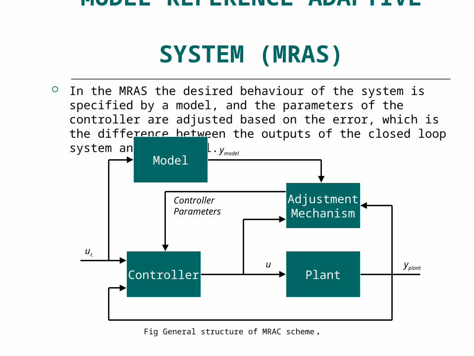
MODEL REFERENCE ADAPTIVE
SYSTEM (MRAS) In the MRAS the desired behaviour of the system is specified by a model, and
the parameters of the controller are adjusted based on the error, which is the difference between the outputs of the closed loop system and the model.
Fig General structure of MRAC scheme.
Controller
Model
AdjustmentMechanism
Plant
Controller Parameters
ymodel
u yplan
t
uc

MODEL REFERENCE ADAPTIVE
SYSTEM (MRAS)Design controller to drive plant response to mimic ideal response Design controller to drive plant response to mimic ideal response (error = yplant-ymodel => 0)(error = yplant-ymodel => 0)Designer chooses: reference model, controller structure, and tuning gains for Designer chooses: reference model, controller structure, and tuning gains for adjustment mechanismadjustment mechanism
References: “ROBUST ADAPTIVE CONTROL” by Petros A. Ioannou & Jing Sun, PTR Prentice -Hall(1996)
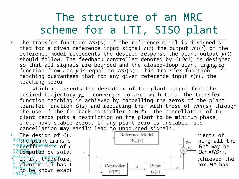
The structure of an MRC scheme for a LTI, SISO plant
The transfer function Wm(s) of the reference model is designed so that for a given reference input signal r(t) the output ym(t) of the reference model represents the desired response the plant output y(t) should follow. The feedback controller denoted by C(Ɵc*) is designed so that all signals are bounded and the closed-loop plant transfer function from r to y is equal to Wm(s). This transfer function matching guarantees that for any given reference input r(t), the tracking error ,
which represents the deviation of the plant output from the desired trajectory ym , converges to zero with time. The transfer function matching is achieved by cancelling the zeros of the plant transfer function G(s) and replacing them with those of Wm(s) through the use of the feedback controller C(Ɵc*). The cancellation of the plant zeros puts a restriction on the plant to be minimum phase, i.e., have stable zeros. If any plant zero is unstable, its cancellation may easily lead to unbounded signals.
The design of C(Ɵc*) requires the knowledge of the coefficients of the plant transfer function G(s). If Ɵ* is a vector containing all the coefficients of G(s) = G(s, Ɵ*), then the parameter vector Ɵc* may be computed by solving an algebraic equation of the form Ɵc* =F(Ɵ*).
It is, therefore, clear that for the MRC objective to be achieved the plant model has to be minimum phase and its parameter vector Ɵ* has to be known exactly.
ye my
1
References: “ROBUST ADAPTIVE CONTROL” by Petros A. Ioannou & Jing Sun, PTR Prentice -Hall(1996)

Direct & indirect MRAC When Ɵ* is unknown the MRC scheme of previous Fig. cannot be implemented because Ɵc
cannot be calculated using Ɵc* =F(Ɵ*) and is, therefore, unknown. One way of dealing with
The unknown parameter case is to use the certainty equivalence approach to replace the
unknown Ɵc* in the control law with its estimate Ɵc(t) obtained using the direct or the indirect
approach .
Fig Direct MRAC
References: “ROBUST ADAPTIVE CONTROL” by Petros A. Ioannou & Jing Sun, PTR Prentice -Hall(1996)
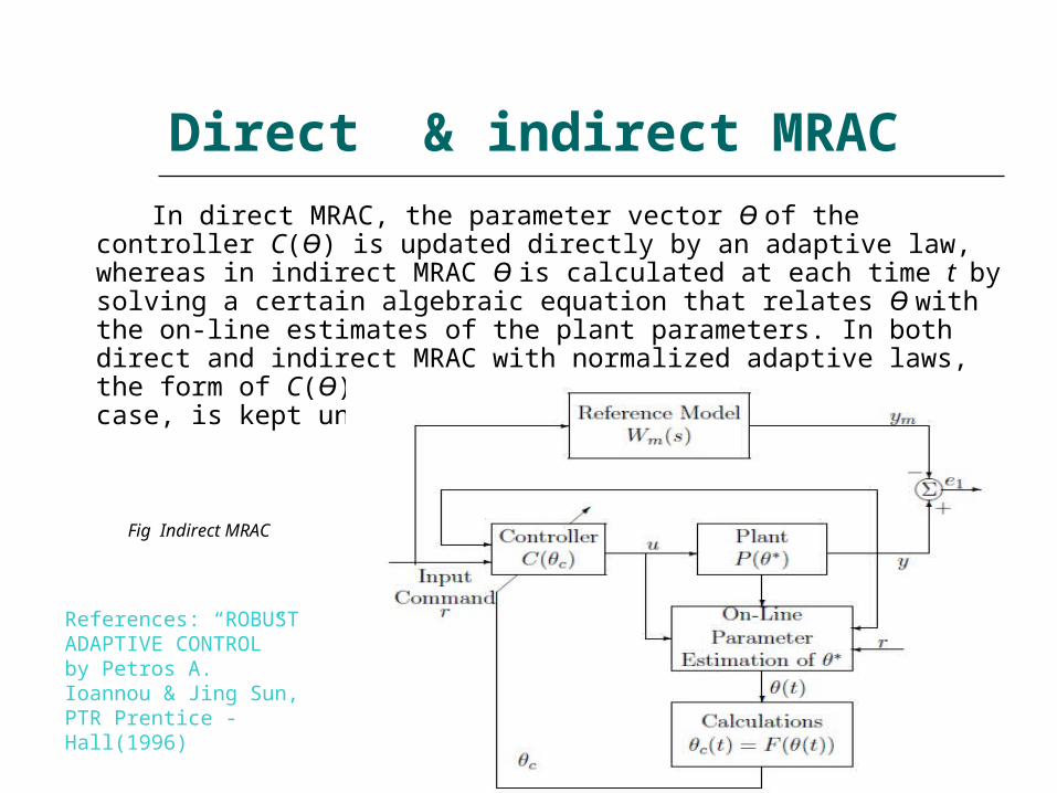
Direct & indirect MRAC In direct MRAC, the parameter vector Ɵ of the controller C(Ɵ) is updated directly by
an adaptive law, whereas in indirect MRAC Ɵ is calculated at each time t by solving a certain algebraic equation that relates Ɵ with the on-line estimates of the plant parameters. In both direct and indirect MRAC with normalized adaptive laws, the form of C(Ɵ), motivated from the known parameter case, is kept unchanged.
Fig Indirect MRAC
References: “ROBUST ADAPTIVE CONTROL” by Petros A. Ioannou & Jing Sun, PTR Prentice -Hall(1996)

MRAC using MIT –rule The MIT rule is the original approach to MRAC. The name is derived from the fact that it was developed
at the Instrumentation Laboratory at MIT. Let us consider a closed loop system in which the controller has one adjustable parameter Ɵ. The desired
closed loop response is specified by a model whose output is ym. let e be the error between the output y of a closed of a closed loop system and the output of the model ym. one possibility is to adjust parameters in such a way that the loss function
is minimized. To make J small, it is reasonable to change the parameters in the direction of
negative gradient of J, that is,
This is known as MIT rule. The partial derivative which is called the sensitivity derivative of the system, tells how the error is influenced by the adjustable parameter. It is assumed that parameters change more slowly than other variables in system. Then the sensitivity derivative can be obtained by assuming Ɵ as a constant.
)(2
1)( 2 eJ
e
e
eJ
dt
d
References: Adaptive control (2nd Edition); Karl Johan Astrom, Bjorn Wittenmark, Prentice Hall

MIT Rule
Can chose different cost functions EX:
From cost function and MIT rule, control law can be formed
0 ,1
0 ,0
0 ,1
)( where
)(
)()(
e
e
e
esign
esigne
dt
d
eJ
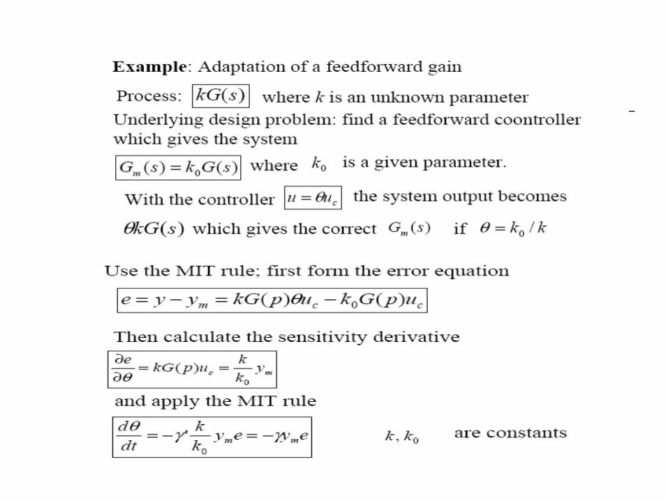
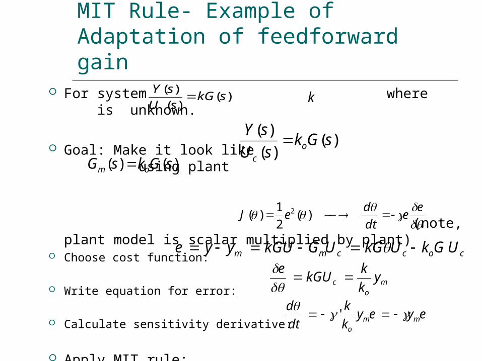
MIT Rule- Example of Adaptation of feedforward gain
For system where is unknown.
Goal: Make it look like using plant
(note, plant model is scalar multiplied by plant)
Choose cost function:
Write equation for error:
Calculate sensitivity derivative:
Apply MIT rule:
)()(
)(skG
sU
sY k
)()(
)(sGk
sU
sYo
c
)()( sGksG om
e
edt
deJ )(
2
1)( 2
coccmm UGkUkGUGkGUyye
mo
c yk
kkGU
e
eyeyk
k
dt
dmm
o
'

block diagram of Adaptation of feedforward gain using mit-rule
Adjustment Mechanism
ymodel
u yplantuc
Π
Π
θ
Reference Model
Plant
s
)()( sGksG om
)()( sGksGp
-
+
considered tuning parameter. Increasing its value leads eventually to oscillations, even stability.
References: Adaptive control (2nd Edition); Karl Johan Astrom, Bjorn Wittenmark, Prentice Hall
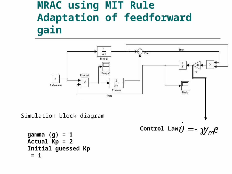
MRAC using MIT Rule Adaptation of feedforward gain
eym
eym Control Law:gamma (g) = 1Actual Kp = 2Initial guessed Kp = 1
Simulation block diagram

Simulation results of MRAC using MIT Rule Adaptation of
feedforward gain
Error between Estimated and Actual value of Kp

Simulation results for MRAC using MIT- rule
Error between Model and Plant

MRAC of Pendulum
TdmgdcJ c 1sin d2
d1dc
T cmgdcsJs
d
sT
s
21
)(
)(
77.100389.0
89.1
)(
)(2
sssT
s
As an exercise in the use of MRAC, the MIT rule (explained in the theory section) was applied to a driven pendulum system. The system contained a vertically oreinted bar whose pivot point was attached to an encoder, so that the angle and angular velocity could be measured. To the end of the bar, a DC motor and propellor were affixed. When voltage was applied to the motor, the propellor spin and pull the bar up. The goal was to command the bar to a specified angle. A diagram of the system is given below:
Newton's laws and conservation of angular momentum were used to derrive the equations of motion. The equations and resulting transfer function for the linearized system are given below:

MRAC of Pendulum
Controller will take form
Controller
Model
AdjustmentMechanism
Controller Parameters
ymodel
u yplant
uc
77.100389.0
89.12 ss
Reference: http://www.pages.drexel.edu/~kws23/tutorials/MRAC/simulation/simulation.html

MRAC of Pendulum
Following process as before, write equation for error, cost function, and update rule
modelplant yye
e
eJ
dt
d
)(2
1)( 2 eJ
It is then assumed that the controller has both an adaptive feedforward (Theta1) and an adaptive feedback (Theta2) gain. To derive expressions for the sensitivity derivatives associated with these parameters, the error function must be restated to invlude Theta1 and Theta2. The equation for the error is first rewritten as the transfer function of the plant and model multiplied by their respective inputs. The input Uc is not a function of either of the adaptive parameters, and therefore can be ginored for now. However, the input U can be rewritten using the feedforward and feedback gains. This can be used to derrive an equation for Yplant.

MRAC of Pendulum
Assuming controller takes the form:
cplant
plantcpplant
cmpmodelplant
plantc
uss
y
yuss
uGy
uGuGyye
yuu
22
1
212
21
89.177.100389.0
89.1
77.100389.0
89.1
plant
c
c
cmc
yss
uss
e
uss
e
uGuss
e
22
1
2
22
12
2
22
1
22
1
89.177.100389.0
89.1
89.177.100389.0
89.1
89.177.100389.0
89.1
89.177.100389.0
89.1
The error can now be written with the adaptive terms included. Taking the partial derivative of the error with respect to Theta1 and Theta2 gives the sensitivity derivatives. Remember that Uc does not include either parameter, and therefore is inconsequential when evaluating the derivative
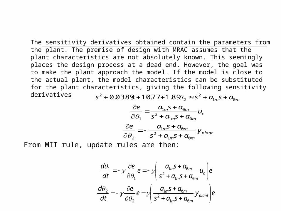
plantmm
mm
cmm
mm
mm
yasas
asae
uasas
asae
asasss
012
01
2
012
01
1
012
22 89.177.100389.0
eyasas
asae
e
dt
d
euasas
asae
e
dt
d
plantmm
mm
cmm
mm
012
01
2
2
012
01
1
1
From MIT rule, update rules are then:
The sensitivity derivatives obtained contain the parameters from the plant. The premise of design with MRAC assumes that the plant characteristics are not absolutely known. This seemingly places the design process at a dead end. However, the goal was to make the plant approach the model. If the model is close to the actual plant, the model characteristics can be substituted for the plant characteristics, giving the following sensitivity derivatives

MRAC of Pendulum
Block diagram
ymodel
e
yplantuc
Π
Π
θ1
Reference Model
Plant
s
77.100389.0
89.12 ss
Π
+
-
mm
mm
asas
asa
012
01
mm
mm
asas
asa
012
01
mm
m
asas
b
012
s
Π
-
+
θ2

Simulation block diagram :Simulation block diagram :
am
s+amam
s+am
-gamma
s
gamma
s
Step
Saturation
omega^2
s+am
Reference Model
180/pi
Radiansto Degrees
4.41
s +.039s+10.772
Plant
2/26
Degreesto Volts
35
Degrees
y m
Error
Theta2
Theta1
y
The controller designed above was implemented. The Simulink block diagram is shown below, along with the The controller designed above was implemented. The Simulink block diagram is shown below, along with the response to a step command of 35 degrees. The transfer function implemented does not exactly mach the transfer response to a step command of 35 degrees. The transfer function implemented does not exactly mach the transfer function stated earlier. There are also several gains added around the plant. This is because the system stated earlier function stated earlier. There are also several gains added around the plant. This is because the system stated earlier assumed an input of a commanded angle. Here, the plant must receive a voltage commandassumed an input of a commanded angle. Here, the plant must receive a voltage command
Reference: http://www.pages.drexel.edu/~kws23/tutorials/MRAC/simulation/simulation.html

Simulation results Simulation with small gamma = UNSTABLE! The plant response obviously doesnt
match the reference model. In fact, the plant almost goes unstable. This response is largely due to the near instability of the open loop system. Tuning of gamma and changing the reference model did not alleviate this problem. In an unconventional attempt to kill the oscillations, proportional and derivative control was applied across the plant.
0 200 400 600 800 1000 1200-100
-50
0
50
100
150
ym
g=.0001

am
s+amam
s+am
-gamma
s
gamma
s
Step
Saturation
omega^2
s+am
Reference Model
180/pi
Radiansto Degrees
4.41
s +.039s+10.772
Plant
1
P
du/dt
2/26
Degreesto Volts
35
Degrees
1.5
D
y m
Error
Theta2
Theta1
y
Solution: Add PD feedbackSolution: Add PD feedback
Reference: http://www.pages.drexel.edu/~kws23/tutorials/MRAC/simulation/simulation.html

Simulation results with varying gammas
The reference model was chosen to have a settling time of 3 seconds and a damping ratio of
.707, which is an industry accepted standard. The plot shows the response for several different
values of gamma. As can be seen, when the value of gamma is increased, the system responds
much faster, but threatens to become unstable. A smaller value of gamma leads to longer
adaptation times, but a less volatile response.
0 500 1000 1500 2000 25000
5
10
15
20
25
30
35
40
45
ym
g=.01
g=.001
g=.0001
707.
sec3
:such that Designed
56.367.2
56.32
s
m
T
ssy

Experimental Resultsof mrac of pendulam
PD feedback necessary to stabilize system.PD feedback necessary to stabilize system.Deadzone necessary to prevent updating when plant approached model.Deadzone necessary to prevent updating when plant approached model.Often went unstable (attributed to inherent instability in system i.e. little Often went unstable (attributed to inherent instability in system i.e. little damping).damping).Much tuning to get acceptable response.Much tuning to get acceptable response.
Reference: http://www.pages.drexel.edu/~kws23/tutorials/MRAC/simulation/simulation.html
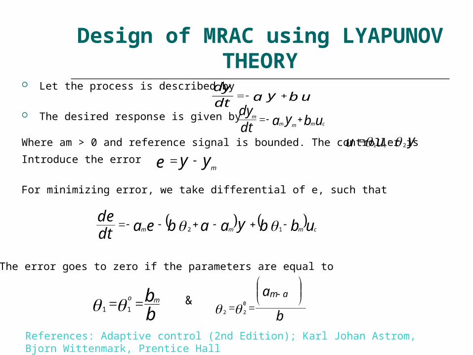
Design of MRAC using LYAPUNOV THEORY
Let the process is described by
The desired response is given by
Where am > 0 and reference signal is bounded. The controller is Introduce the error
For minimizing error, we take differential of e, such that
The error goes to zero if the parameters are equal to
ubyadtdy
ubyadtdy
cmmmm
yuu c 21
yye m
ubbyaabeadtde
cmmm 12
bbmo 11
b
a am
0
22
&
References: Adaptive control (2nd Edition); Karl Johan Astrom, Bjorn Wittenmark, Prentice Hall

Design of MRAC using LYAPUNOV THEORY
Now a parameter adjustment mechanism is constructed that will drive the parameters Ɵ1; Ɵ2 to there desired values. For this purpose, let us assume that > 0 and introduce the following quadratic function
This function is zero when e is zero and the controller parameters are equal to correct values.
For function to be a Lyapunov the derivative must be negative. The derivative is
b
2
1
2
2
1122
121,, bbbaabeeV mmb
dt
de
dtdbbdt
daab
dtde
edtdV
mm
1
1
122
1
References: Adaptive control (2nd Edition); Karl Johan Astrom, Bjorn Wittenmark, Prentice Hall

Design of MRAC using LYAPUNOV THEORY
If the parameters are updated as
eudtdbbye
dtd
aabeadtdV
cm mm
1
1
122
12
eudtd
c 1
yedtd 2
And we get
eadtdV
m
2
The derivative of V is thus negative semidefnite but not negative definite. This implies that V(t) ≤ V(0) and that e, Ɵ1 and Ɵ2 must be bounded. This implies that y = e + ym
also is bounded. Since uc , e, and y are bounded, it follows is bounded. Hence
dV/dt is uniformly continous.V
..

Block diagram of MRAC using LYAPUNOV THEORY
References: Adaptive control (2nd Edition); Karl Johan Astrom, Bjorn Wittenmark, Prentice Hall

MULTIVARIABLE SYSTEM
A continuous stirred tank reactor (CSTR) is used to convert a reactant (A) to a product (B). The reaction is liquid phase, first order and exothermic. Perfect mixing is assumed. A cooling jacket surrounds the reactor to remove the heat of reaction. In this system variables of interest (from a control engineers perspective) could be, for example, product composition and temperature of the reacting mass. There will therefore be a composition control loop as well as a temperature control loop. Feed to the reactor is often used to manipulate product composition while temperature is controlled by adding (removing) energy via heating (cooling) coils or jackets. This basic control configuration is demonstrated in Fig (1). 'TC' represents a temperature controller, the mv for this loop being coolant flowrate to the jacket. 'CC' represents the composition controller, the mv being reactant feedrate.
References: Multivariable Control: An introduction, Dr M.J. Willis: Department of Chemical and Process Engineering, University of Newcastle upon Tyne

Input-Output Multivariable System
Models: Here G11(s) is a symbol used to represent the forward path dynamics between mv1 and cv1, while
G22(s) describes how cv2 responds after a change in mv2. The interaction effects are modelled using transfer functions G21(s) and G12(s). G21(s) describes how cv2 changes with respect to a change in mv1 while G12(s) describes how cv1 changes with respect to a change in mv2.
For the CSTR shown in above figure mv1 could be the coolant flowrate, while mv2 could be the flowrate of the reactant. The output cv1 may be the reactor temperature while the output cv2 would be the effluent concentration.
The mathematical model written in matrix-vector notation: on a loop by loop basis, the outputs of the system model are related to the inputs as follows,
Loop 1: cv1 = G11 mv1 + G12mv2 ; Loop 2: cv2= G21mv1 + G22 mv2 or cv = G mv
where cv = [cv1, cv1]T mv = [mv1 mv2 ]T
G=
GGGG
2221
1211
and, G=
References: Multivariable Control: An introduction, Dr M.J. Willis: Department of Chemical and Process Engineering, University of Newcastle upon Tyne

Adaptive Control for Multivariable Plants
Decentralized Adaptive Control: Let us consider the MIMO plant model
Where y € RN , u ϵ RN and H(s) ϵ CN*N is the plant transfer matrix that is assumed to be proper.
Where hij , the elements of H(s), are transfer function.
For some different hij(s) and qij(s). If the MIMO plant model is such that the interconnecting orcoupling transfer functions hij(s);qij(s). (I j) are stable and small in some sense, then they can be treated as modelling error terms in the control design. This means that instead of designing an adaptive controller for the MIMO plant (3), we can design N adaptive controllers for N SISO plant models of the form
References: “ROBUST ADAPTIVE CONTROL” by Petros A. Ioannou & Jing Sun, PTR Prentice -Hall(1996)

MRAC FOR MULTIVARIABLE
Consider the MIMO plant y=G(s)u (1)where yϵ RN, uϵ RN and G(s) is N*N transfer matrix. The reference model to be matched by the
closed-loop plant is given by ym =Wm(s)r (2)where ym,rϵ RN Because G(s) is vector transfer function. The following Lemma is used to
define the counterpart of the high frequency gain and relative degree for MIMO plants.
Lemma (1) : For any N*N strictly proper rational full rank transfer ma-
References: “ROBUST ADAPTIVE CONTROL” by Petros A. Ioannou & Jing Sun, PTR Prentice -Hall(1996)

To meet the control objective we make the following assumptions about
the plant:
A1. G(s) is strictly proper, has full rank and a known MLI matrix (s)
A2. All zeros of G(s) are stable.
A3. A matrix Sp that satisfies KpSp = (KpSp)T > 0 is known. Furthermore we assume that the transfer matrix Wm(s) of the reference model is
designed to satisfy the following assumptions:
Tao, G. and P.A. Ioannou, “Robust Model Reference Adaptive Control for Multivariable Plants," International Journal of Adaptive Control and Signal Processing, Vol. 2, no. 3, pp. 217-248, 1988.

DESIGN of MRAC for Multivariable system
We can design a MRAC scheme for the plant (1) by using the certainty equivalence approach by assuming that all the parameters of G(s) are known and propose the control law
o(s) is a monic Hurwitz polynomial of degree
.
K p
1The closed-loop plant transfer matrix from y to r is equal to Wm(s) provided Ɵ3
*= and Ɵ1*; Ɵ2*
are chosen to satisfy the matching equation
(3)
(4) Tao, G. and P.A. Ioannou, “Robust Model Reference Adaptive Control for Multivariable Plants," International Journal of Adaptive Control and Signal Processing, Vol. 2, no. 3, pp. 217-248, 1988.
CONTINUE…………………..
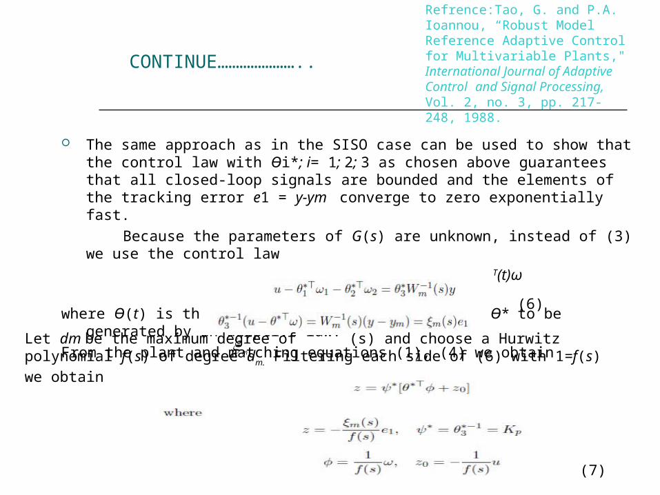
The same approach as in the SISO case can be used to show that the control law with Ɵi*; i= 1; 2; 3 as chosen above guarantees that all closed-loop signals are bounded and the elements of the tracking error e1 = y-ym converge to zero exponentially fast.
Because the parameters of G(s) are unknown, instead of (3) we use the control law
u = Ɵ T(t)ω (5)
where Ɵ(t) is the on-line estimate of the matrix Ɵ* to be generated by an adaptive law.
From the plant and matching equations (1), (4) we obtain
(6)
mLet dm be the maximum degree of (s) and choose a Hurwitz polynomial f(s) of degree dm. Filtering
each side of (6) with 1=f(s) we obtain
(7)
Refrence:Tao, G. and P.A. Ioannou, “Robust Model Reference Adaptive Control for Multivariable Plants," International Journal of Adaptive Control and Signal Processing, Vol. 2, no. 3, pp. 217-248, 1988.

CONTINUE…………………..
Generated the estimated value of z,
and the estimation error
Refrence:Tao, G. and P.A. Ioannou, “Robust Model Reference Adaptive Control for Multivariable Plants," International Journal of Adaptive Control and Signal Processing, Vol. 2, no. 3, pp. 217-248, 1988.

Multivariable nonlinear model reference control of cement
mills The dynamical model of the system is described by three coupled and nonlinear differential
equations as given in (1)–(3). The states of the system are characterized by the mill load denoted by z (in tons), the product flow rate denoted by yf (in tons/h) and the tailings flow rate denoted by yr (in tons/h). On the other hand, w is the output flow rate of the mill and d denotes the relative hardness of the material inside the mill with respect to the nominal one, which is unity. The system has two control inputs, denoted by u (tons/h), the feed flow rate and, v (rpm), the classifier speed
yudzz r
,
dzdvzyyT ff f ,,,1
dzdvzyyT rr r ,,,
(1)
(2)
(3)
The variables Tf and Tr stand for the time constants for product flow rate and tailings flow rate dynamics, respectively.
(4)
References: Mehmet Onder Efe, “Multivariable nonlinear model reference control of cement mills,” Transactions of the Institute of Measurement and Control 25,5 (2003), pp. 373–385

Schematic diagram of the cement milling circuit
References: Mehmet Onder Efe, “Multivariable nonlinear model reference control of cement mills,” Transactions of the Institute of Measurement and Control 25,5 (2003), pp. 373–385

The control problem is to enforce the system states to follow the states of a reference model by
appropriately altering the two control inputs.
Reference model: In choosing the reference dynamics for z and yf, we assume
1) The reference model for each state, whose variables are represented with a subscript m, must be stable and must follow the command signal. Since the differential equations in (1)-(3) are of first order, we choose the corresponding reference dynamics as a first-order system;
2) The response imposed by the reference system must not be faster than what could be achieved by the actual system, i.e., the time constants must be compatible.
Denote the command signals for reference mill load (zm) and the reference product flow rate (ymf ) states by r and f, respectively. If for some tc 0, zm (tc ) = r(tc) is satisfied, then (5) is
satisfied for all t tc.
Two out of three state variables are kept under control; the behaviour of the third state is determined by the first two.
Refrence:Tao, G. and P.A. Ioannou, “Robust Model Reference Adaptive Control for Multivariable Plants," International Journal of Adaptive Control and Signal Processing, Vol. 2, no. 3, pp. 217-248, 1988.

Synthesis of the control signal for cement mill

Simulation results:
In the upper subplot of Figure, the command signal (r), the response of the reference model (zm) and the response of the system are illustrated together. After approximately 5 h, the value of the plant output comes admissibly close to that of the model output. In order to clarify the tracking claim, the lower subplot depicts the model following error in state z. The variation in the plant output is due to the uncertainty on the relative material hardness parameter.
Refrence:Tao, G. and P.A. Ioannou, “Robust Model Reference Adaptive Control for Multivariable Plants," International Journal of Adaptive Control and Signal Processing, Vol. 2, no. 3, pp. 217-248, 1988.

Recent development in mrac
Modified MRAC methods Fuzzy-MRAC Variable Structure MRAC (VS-MRAC) Robust multiple model adaptive control (RMMAC)

Brief History: Generated Library of Tools 1960s
Sensitivity Method, MIT RuleLimited stability analysis
Whitaker, Kalman, Parks, …1970s
Lyapunov basedPassivity based
Morse, Narendra, Landau, …
Late 1970s - 1980s
Global stabilityMorse, Narendra, Egardt, Landau, Goodwin,
Keisselmeier, Anderson, Astrom….
Early 1980s
Robustness issues, InstabilityEgard, Rohrs, Ioannou, Athans, Anderson,
Astrom, …
1980s
Robust adaptive control Praly, Ioannou, Narendra, Tsakalis, Annaswamy,
Sun, Tao, Goodwin, Middleton etc
1990s
Nonlinear adaptive control
1990s
Search methods, Multiple models, Switching
techniquesMartenson, Miller, Barmish,Morse,Narendra,
Morse, Andreson, Safonov, ….
Adaptive backstepping
Krstic, Kanelakopoulos, Kokotovic, Zhang, …
Neuro-Adaptive control
Fuzzy-Adaptive controlNarendra, Lewis, Polycarpou,
Kosmatopoulos, Xu, Ioannou, Wang,
Lavresky, Hovakimyan …

A New Toolbox for use with MATLAB® and Simulink® [P.A. Ioannou & B. Fidan]
• Parameter Identification
• Adaptive Control
in both Continuous-Time and Discrete-Time
Parameter Identification
• Gradient Methods
• Least-Squares Methods
• SPR-Lyapunov Approaches(Adaptive) Control
• Model Reference (Adaptive) Control• Direct, Indirect
• (Adaptive) Pole Placement Control• Polynomial, State-Variable, Linear Quadratic
• Minimum Prediction Error Control• Direct, Indirect, Semi-direct
Adaptive Law Modifications• Normalization
• Static, Dynamic
• Parameter Projection
• Robustness Modifications• σ, ε, Dead-zone
Other
• (Adaptive) State Estimation
• Output Prediction (ARMA)
• Parametric Model Order Reduction
• Polynomial Algebra
Adaptive control toolbox

Simulink® Blocks:
MATLAB® Commands:
zu
yPlant I/O
Signals
ParametricModel Signals
z
dn
ParameterEstimate
Parametric Model Signals
Normalizing Signal
uy
Plant I/OSignals Parameter
Estimate
z rz
r
OriginalParametric Model
Signals
Reduced-OrderParametric Model Signals
Gradient Methods:Function Purposeucgrad,ucgradbk,ucgradint Continuous-time gradient algorithms dgradb, dgradl, udgrad Discrete-time gradient algorithms dprojmod, dprojorth, Discrete-time projection algorithms dprojpure, udproj
Least-Squares (LS) Methods:Function Purposeucrls, urlsarg Continuous-time LS algorithmsdrls, udrls, urlsarg Discrete-time LS algorithms
Model Conversion/Model Order Reduction:Function Purposeutf2lm, io2lm Transfer function to linear parametric model uarma2lm, io2lm ARMA to linear parametric model lmred Parametric model order reduction
dnNormalizing Signal
On line Parameter Estimators

Simulink® Block:
MATLAB® Commands:
r
uyPlant Output Control Signal
z
dnParameter Estimate
Parametric Model SignalsDynamic Normalizing Signal
Model Reference Adaptive Control (MRAC):Function Purposemrcpoly MRC/MRAC design – Polynomial Approach dmrc Discrete-time MRC/MRAC design umrcdrb, umrcdrl Continuous-time direct MRAC umrcidr Continuous-time indirect MRACudmracdr Discrete-time direct MRAC udmracidr Discrete-time indirect MRAC
One-Step Ahead Adaptive Control (OSAAC):(Discrete Time)Function Purposedosac OSAC/OSAAC designudosacdr Direct OSAACudosacidr Indirect OSAACudosaclcf OSAAC – Linear control form approach
Adaptive Pole Placement Control (APPC):Function Purposeppcpoly, ppcssv Continuous-time PPC/APPC design dppcdo, dppcimp, Discrete-time PPC/APPC design dppcdo, dppcimpppcclq Continuous-time (adaptive) LQC design ppcdlq Discrete-time (adaptive) LQC design uppcpoly, uppcrsf PPC/APPC & (adaptive) LQC implementation
Polynomial Algebra Tools:Function Purposebezout, diophant Solving Diophantine equations euclid Greatest common divisor of two polynomialspolylcm Lowest common multiple of two polynomials
Reference Signal
Adaptive control

• Numerical implementation of an extensive set of parameter identification and adaptive control schemes.
• Simulink® blocks with user-friendly GUIs to implement the schemes and to select/tune the design parameters easily.
• Ability to implement the same schemes using the provided MATLAB® commands in order to have flexibility.
• Applicability to both continuous-time and discrete-time plants.
• Normalization, parameter projection, and robust modification capabilities to guarantee stability and robustness.
• Basic polynomial algebra tools to design controllers based on model matching and pole placement techniques.
% Process: for k = 1:N_final-1, theta(:,k) = ucrls('parameter',x_est,ntheta); [thetau, thetay, thetar, RETYPE] = mrcpoly(theta(1,k),… [1 theta(2,k)],Zm,Rm,Lambda_c); theta_c(:,k) = [thetau(:); thetay(:); thetar(:)]; u(k) = umrcidr('control',xc,[y(k) r(k)],[n m],Lambda_c,Lambda_p,theta_c(:,k)); dxc = umrcidr('state',xc,[u(k) y(k)],[n m],Lambda_c,Lambda_p); [z(k), phi(:,k)] = umrcidr('output', xc,[u(k) y(k)],[n m],Lambda_c,Lambda_p); xc = xc + dxc*dt; dxp = ufilt('state', xp, u(k), b, a); y(k+1)= ufilt('output',xp, u(k), b, a); xp = xp + dxp*dt; dxm = ufilt('state', xm, r(k), Zm, Rm); ym(k+1)= ufilt('output', xm, r(k), Zm, Rm); xm = xm + dxm*dt; dx_est = ucrls('state', x_est,z(k),phi(:,k), 0,ArgLS,[],[]); x_est = x_est + dx_est*dt;end
Key features
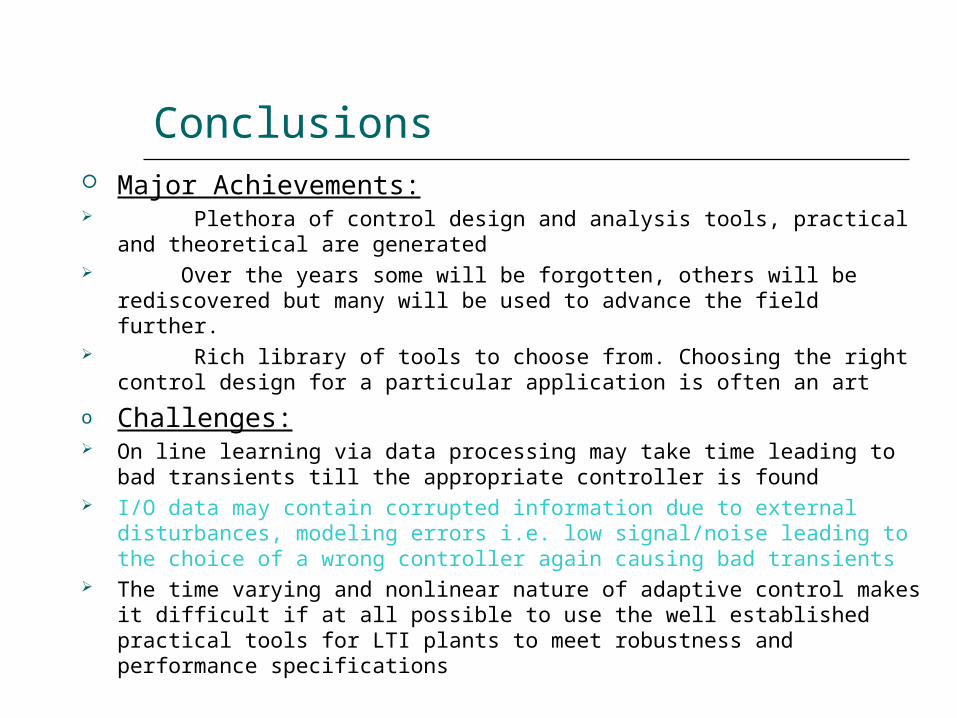
Conclusions Major Achievements: Plethora of control design and analysis tools, practical and theoretical are generated Over the years some will be forgotten, others will be rediscovered but many will be used to
advance the field further. Rich library of tools to choose from. Choosing the right control design for a particular
application is often an art
o Challenges: On line learning via data processing may take time leading to bad transients till the appropriate
controller is found I/O data may contain corrupted information due to external disturbances, modeling errors i.e.
low signal/noise leading to the choice of a wrong controller again causing bad transients The time varying and nonlinear nature of adaptive control makes it difficult if at all possible to
use the well established practical tools for LTI plants to meet robustness and performance specifications

references
Astrom K.J.and Bjorn Wittenmark, Adaptive control, Prentice Hall, Second edition, India, 2001.
Petros A. Ioannou & Jing Sun, Robust adaptive control, PTR Prentice Hall(1996) Astrom, K.J., “Theory and Applications of Adaptive Control-A Survey,"
Automatica, Vol. 19, no. 5, pp. 471-486, 1983. Tao, G. and P.A. Ioannou, “Robust Model Reference Adaptive Control for
Multivariable Plants," International Journal of Adaptive Control and Signal Process g, Vol. 2, no. 3, pp. 217-248, 1988.
Dr M.J. Willis, Multivariable Control: An introduction, Department of Chemical and Process Engineering, University of Newcastle upon Tyne.
Mehmet Onder Efe, “Multivariable nonlinear model reference control of cement mills,” Transactions of the Institute of Measurement and Control 25,5 (2003), pp. 373–385.
Petros Ioannou, University of Southern California, Los Angeles Robust Adaptive Control : The Search for the Holy Grail (ppt.)
http://www.pages.drexel.edu/~kws23/tutorials/MRAC/simulation/simulation.html MATLAB 7.0.1 (Adaptive control tool box)
