model order reduction for discrete unstable control ... order reduction for discrete unstable...

School of Mathematics, Meteorology and Physics

Department of Mathematics

Preprint MPS_2010-06

18 March 2010

Model order reduction for discrete unstable control systems using a balanced truncation

approach

by

C. Boess, N.K. Nichols and A. Bunse-Gerstner

Model order reduction for discrete unstable control systems

using a balanced truncation approach

C. Boess∗, N.K. Nichols∗ and A. Bunse-Gerstner†

Abstract

Mathematical modeling of problems occurring in natural and engineering sciencesoften results in a very large dynamical system. Efficient techniques for model orderreduction are required, therefore, to reduce the complexity of the system. Almost allsuch techniques require the dynamical system to be asymptotically stable. Balancedtruncation is a well-known and approved model reduction method. There alreadyexists a simple approach for applying this technique to unstable systems, but it doesnot capture the full behavior of the system successfully. In this paper, we proposea new model reduction method based on α-bounded balanced truncation, which canbe applied to unstable systems independently of the number of unstable poles. Weestablish that this new method computes a low order approximation to the full ordersystem such that the corresponding error system is close to being optimal with respectto a well-defined norm for unstable systems. Moreover, we prove a global error boundfor the error system. In numerical experiments with unstable test models we comparethe new α-bounded balanced truncation method with the standard extension of bal-anced truncation for unstable systems. The results show the superior performance ofthe α-bounded method.

Keywords: Model order reduction, unstable systems, balanced truncation, control

1 Introduction

Reduced order modeling is a crucial concept within the study of dynamical systems. Thepurpose of model order reduction is to reduce the order of the system substantially whilestill capturing its most important properties. Most of the known model reduction tech-niques are for asymptotically stable systems only, but in many fields of applications largeunstable systems do occur and an order reduction is required. For example to be able tomake a reliable weather forecast high resolution models of the atmosphere are indispens-able. These models generally contain a large number of unstable modes. Moreover, thelarge dimensions of these unstable systems - usually about 107 unknowns are involved -require efficient techniques to reduce the order of the model considerably without losingessential information. In this paper we propose a new concept for reducing the order ofdiscrete-time unstable systems while still capturing the most important information tomatch the input-output behavior of the original full order model. Similar results can beestablished for continuous-time systems (see [12]). Our focus is on a balanced truncationtype method because this is an approved and reliable technique for reducing the order ofdynamical systems. However, our new approach can also be applied within other model

∗[email protected] (corresponding author), [email protected], Department of Mathe-matics, University of Reading, Caroline Boess acknowledges support by NCEO

†[email protected], ZeTeM, Universitaet Bremen

1

reduction methods, including rational interpolation and Kyrlov subspace methods, see e.g.[12].

Originally, the balanced truncation method was proposed for asymptotically stablecontinuous-time systems by Moore in 1981 [14]. Pernebo and Silverman [16] extendedthe method to discrete-time systems in 1982. There already exist some extensions of thestandard method to unstable systems. Most of these methods are based on an additivedecomposition separating the asymptotically stable from the unstable part of the system.These techniques assume that unstable poles cannot be neglected when modeling thedynamics of a system, see e.g. [7, pp. 1177-1178], [15, 10, 19] and the references therein.

The main disadvantage of all methods based on this idea is that they are very limitedwhen the system has a large number of unstable poles. A reduction of the full order systemto a reduction order smaller than the number of unstable poles supplies a low order modelwhich can only keep some of the unstable modes while the asymptotically stable partis ignored completely. Thus, this procedure cannot supply a good approximation of theinput-output behavior of the whole full order system but only of its unstable part.

In this paper we propose a new approach to approximate discrete unstable controlsystems by systems of lower order using a balanced truncation technique. In contrastto existing approaches, this new method approximates the input-output behavior of theasymptotically stable as well as of the unstable part of the full order system, no matterhow many unstable poles there are. The main idea is to extend the balanced truncationmethod to unstable systems by considering a different norm in which the error system ismeasured.

Usually, balanced truncation for asymptotically stable systems computes a low ordersystem such that the output error is close to being optimal in the h2-Hardy-norm [4, 5].This norm is only well-defined for asymptotically stable systems. There exists an extensionto unstable systems, the so-called h2,α-norm [9, 5]. We use this extended norm to definea new balanced truncation method for unstable systems where the output error is thenclose to being optimal in the h2,α-norm. Moreover, we derive a global error bound for thenew balanced truncation method.

The outline of this paper is as follows. Section 2 gives a brief introduction to themodel reduction method of balanced truncation for asymptotically stable discrete systemssummarizing its most important properties. It also presents the main ideas of the stan-dard extension to unstable systems. In Section 3 this is followed by the proposition ofa new model reduction approach for unstable systems, the α-bounded balanced trunca-tion method. Finally, Section 4 contains results of various numerical experiments usingthree different unstable discrete test models. We compare our new method of α-boundedbalanced truncation with the already existing balanced truncation approach for unstablesystems. The paper concludes with a summary of our results.

2 Reduced order modeling for discrete systems using bal-

anced truncation

We investigate discrete linear time-invariant systems of the form

S :

{xi+1 = Axi + Bui,yi = Cxi,

(1)

with state xi ∈ Rn, input ui ∈ R

m, output yi ∈ Rp, system matrix A ∈ R

n×n, input matrixB ∈ R

n×m, output matrix C ∈ Rp×n and zero initial state x0 = 0. A good and compact

way to describe the input-output behavior of the system can be achieved by applying the

2

Z-transform to the system (1):

zX(z) = AX(z) + BU(z),Y (z) = CX(z),

(2)

where X(z), U(z), Y (z) are the Z-transforms of xi, ui, yi, respectively. Rewriting (2) weobtain

Y (z) =(C(zI − A)−1B

)U(z). (3)

2.1 DefinitionFor a discrete linear system S of the form (1) the function

G(z) := C(zI − A)−1B (4)

is known as the transfer function.

Equation (3) shows that the transfer function relates inputs to outputs in frequency do-main. In the following we consider discrete linear systems which are in general unstable.

2.2 DefinitionA discrete linear system S of the form (1) is called asymptotically stable if all eigenvaluesof the system matrix A lie inside the unit disk D := {x ∈ C | |x| < 1}.

The dimension n of the system matrix A is known as the order of the dynamical system(1). We consider problems where the order is typically very large. Techniques to reducethe order of the system are indispensable. The main idea of model reduction methods isto approximate the system (1) by a system of much smaller order k ≪ n:

S :

{xi+1 = Axi + Bui,

yi = Cxi,(5)

with reduced state xi ∈ Rk, input ui ∈ R

m, output yi ∈ Rp, reduced system matrix

A ∈ Rk×k, reduced input matrix B ∈ R

k×m and reduced output matrix C ∈ Rp×k. The

aim of model reduction is to find a low order system S of order k ≪ n such that theresponse yi of S is as close as possible to the response yi of the full order system S.

One approach to finding a low order system S that approximates the input-outputbehavior of the full order system S is to minimize the distance between the transferfunctions of the full and low order system in a suitable norm:

‖G − G‖ = min! (6)

where G and G are the transfer functions of S and S, respectively.The minimization of (6) will also assure that the outputs of the low order system are

not too far from the outputs of the full order system due to the following relation betweeninputs and outputs in frequency domain:

‖Y (z) − Y (z)‖ = ‖(

G(z) − G(z))

U(z)‖ ≤ ‖G(z) − G(z)‖‖U(z)‖, (7)

where Y (z), Y (z) and U(z) are the Z-transforms of yi, yi and ui, respectively.Before specifying a suitable norm for the minimization (6) we first have a closer look

at the output. The output of the system (1) after ℓ time steps is given by:

yℓ = CAℓℓ∑

j=1

A−jBuj−1.

3

This leads to the following description of the output in frequency domain:

Y (z) =

∞∑

ℓ=0

yℓ z−ℓ

= C∞∑

ℓ=0

ℓ∑

j=1

z−ℓAℓ−jBuj−1. (8)

Thus, we see that Y (z) is only a finite number if the absolute value of z is largerthan the largest eigenvalue of A in absolute value. As a consequence, the inequality (7)is only well-defined for |z| > α where α is an upper bound for the largest eigenvalue ofA in absolute value. This observation has to be taken into account when choosing anappropriate norm for the minimization (6).

For asymptotically stable systems α = 1 is an upper bound for the absolute value ofall eigenvalues. This justifies the use of the h2-norm as defined in [9, 1]:

2.3 DefinitionWe consider the space

M (q,s) := {F : DC → Cq×s | F is holomorphic in DC}

where DC denotes the complement of the closed unit circle. For any element F ∈ M (q,s)

the corresponding h2-norm is defined as:

‖F‖h2:=

(

1

2πsup|r|>1

∫ 2π

0trace

[

F ∗(re−ıθ)F (reıθ)]

dθ

) 1

2

.

It is crucial for this norm to be well-defined that the supremum is only considered overradii r which have an absolute value that is larger than all eigenvalues of A in absolutevalue. For asymptotically stable systems this is always fulfilled because all eigenvalues aresmaller than one in absolute value. We will see in Section 3 how this insight motivatesthe use of a generalized h2-norm when considering unstable systems.

We now focus on model reduction methods for asymptotically stable systems thatminimize the difference between the transfer functions of the full and the low order modelwith respect to the h2-norm:

‖G − G‖h2= min! (9)

There already exist several approaches for computing a reduced order system S suchthat (9) is minimized. Necessary conditions for such a minimum are established in [4]. Itis not practicable to find the optimal reduced model matrices that satisfy these conditions,however, as large systems of nonlinear equations must be solved. Instead we concentrateon the method of balanced truncation - an approved technique for model reduction ofasymptotically stable linear systems. Its main idea is to truncate the states of the systemthat are least influenced by the inputs and have least effects on the outputs. This isonly possible if the system has been transformed to balanced form first. The balancedtruncation method then computes a reduced order system which is close to being optimalin the sense that the h2-norm difference of the transfer functions (9) is approximatelyminimized [4].

The response of a discrete linear system is represented by its Hankel matrix. Balancedtruncation computes the reduced order system S in such a way that the Hankel singularvalues of the full linear model are retained. We refer to [3, 18] for more computationaldetails. A main advantage of this model reduction technique is that there exists a globalbound for the error between the transfer function of the original and the low order model.

4

2.4 Theorem:Let S be a system of the form (1) with corresponding transfer function G. Moreover, let

S with corresponding transfer function G be a reduced system of the form (5) with orderk < n that is computed using balanced truncation. Then the following bound for the errorsystem holds:

‖G − G‖h∞≤ 2(σr+1 + . . . + σn), (10)

where σi are the Hankel singular values of the original system. The h∞-norm is definedas

‖G‖h∞:= sup

θ∈[0,2π]σmax

(

G(eiθ))

,

where σmax denoted the largest singular value.

Proof: We refer to [9]. �

Balanced truncation requires the linear system (1) to be asymptotically stable. Other-wise the system cannot be transformed to balanced form. However, as briefly stated in theintroduction, there exist extensions to unstable systems. They are based on an additivedecomposition of the system into its asymptotically stable and its unstable part:

G = G+ + G− ,

where G+ and G− are the transfer function of an asymptotically stable and an unstablesubsystem, respectively. Once this additive stable-unstable decomposition of G is foundthen the original balanced truncation technique for asymptotically stable systems can beapplied to G+. In this procedure the unstable part G− remains unchanged. Finally, thereduced stable part is recomposed with the unchanged unstable part. In general, thismodel reduction procedure for unstable systems can only work well if the system has asmall number of unstable poles. The attempt to reduce the order of the system to anorder smaller than the number of unstable poles leads to a low order system that onlykeeps a part of the unstable subsystem G−. It is not even assured that at least themost dominant part of G− should be kept. Additionally, the asymptotically stable part isignored completely. For further details on this method we refer to [7, 15, 10, 19].

The following section proposes a new balanced truncation approach for unstable sys-tems which takes into account the asymptotically stable as well as the unstable part ofthe full order system.

3 Balanced truncation for unstable α-bounded systems

An important property of balanced truncation for asymptotically stable systems is thatit computes a low order system such that the h2-norm difference of the transfer functionsof the full and the reduced order systems (9) is close to being optimal. As the h2-norm isonly defined for asymptotically stable systems we cannot aim to get the same result whenconsidering unstable systems. However, we are able to derive a similar property for ournew method for unstable systems. As mentioned in the previous section the common hp-norms are only well-defined if all eigenvalues of the system matrix lie inside the unit circle.Moreover, we have shown that using the inequality (7) as a basis for the approximationof the original system (1) is only reasonable for |z| > α, where α is an upper bound forthe largest eigenvalue in absolute value. This insight motivates a natural generalizationof standard hp-norms to unstable systems as proposed in [9].

5

3.1 Definition (hp,α-norms)Let α be a real positive number. For any element

F ∈ M(p,m)α := {F : DC

α → Cp×m|F is holomorphic in DC

α },

where DCα is the complement of the closed circle around the origin with radius α, the

corresponding h2,α- and h∞,α-norms are defined as:

‖F‖h2,α:=

(

1

2πsup|r|>α

∫ 2π

0trace

[

F ∗(re−ıθ)F (reıθ)]

dθ

) 1

2

=

(1

2π

∫ 2π

0trace

[

F ∗(αe−ıθ)F (αeıθ)]

dθ

) 1

2

and

‖F‖h∞,α:= sup

z∈DCα

σmax (F (z))

= supθ∈[0,2π]

σmax

(

F (αeiθ))

,

where σmax denotes the largest singular value.

We note that the special case of the hp,α-norm where α is equal to one supplies thestandard hp-norm. The main advantage of the hp,α-norm is that it is well-defined forunstable systems if the value of α is chosen such that all eigenvalues of the system matrixA of the system (1) lie inside a disk around the origin with radius α.

3.2 Definition (α-boundedness)Let α ∈ R be a positive number. Then a discrete control system S of the form (1) is calledα-bounded if all eigenvalues of the system matrix A lie inside a disk around the originwith radius α, i.e.

λ eigenvalue of A ⇒ λ ∈ Dα

with Dα := {x ∈ C | |x| < α}.

We note that for α = 1 the concept of α-boundedness is equivalent to asymptotic stability.For a regular discrete (in general) unstable system of the form (1) it is always possible tofind real positive numbers α such that the system is α-bounded. In general α-boundedsystems are not asymptotically stable. Thus, the standard hp-norm is not well-defined,but the hp,α-norm is.

Using this generalized norm for unstable systems, we now derive a new α-boundedbalanced truncation method. To determine a suitable α, a rough knowledge of the eigen-structure of the system matrix A is needed. This can be achieved using a simple iterativemethod for computing the largest eigenvalue in absolute value, such as the Arnoldi method,or using the concept of Gershgorin circles, see e.g. [8, 17, 2, 6]. Once a suitable α isdetermined the following shift of the original system is considered.

3.3 LemmaFor any linear discrete, reachable and observable α-bounded system S of the form (1) weconsider the shifted system

Sα :

{

x(α)i+1 = Aαx

(α)i + Bαui,

y(α)i = Cαx

(α)i ,

(11)

6

with Aα := A/α, Bα := B/√

α and Cα := C/√

α. Let G and Gα be the correspondingtransfer functions of (1) and (11), respectively. Then the following properties hold:

(i) Sα is asymptotically stable.

(ii) The h2−norm of Sα is equal to the h2,α−norm of S:

‖Gα‖h2= ‖G‖h2,α

.

(iii) The h∞−norm of Sα is equal to the h∞,α−norm of S:

‖Gα‖h∞= ‖G‖h∞,α

.

Proof:

(i) It is a well-known result from linear algebra that the eigenvalues of the matrix Aα

are the eigenvalues of A divided by α. This implies the statement.

(ii) It holds that

Gα(eıθ) = Cα

(

e−ıθI − Aα

)−1Bα

=C√α

(

e−ıθI − A

α

)−1 B√α

=C√α

(1√α

(αe−ıθI − A)1√α

)−1 B√α

= C(αe−ıθI − A)−1B

= G(αeıθ),

and thus,

‖Gα‖h2=

(1

2π

∫ 2π

0trace

[

G∗α(e−ıθ)Gα(eıθ)

]

dθ

) 1

2

=

(1

2π

∫ 2π

0trace

[

G∗(αe−ıθ)G(αeıθ)]

dθ

) 1

2

= ‖G‖h2,α.

(iii) Then it also holds that

‖Gα‖h∞= sup

θ∈[0,2π]σmax

(

Gα(eiθ))

= supθ∈[0,2π]

σmax

(

G(αeiθ))

= ‖G‖h∞,α,

where σmax denotes the largest singular value.

�

Given a discrete linear system S of the form (1) our new balanced truncation approachfor unstable systems can be stated as follows:

7

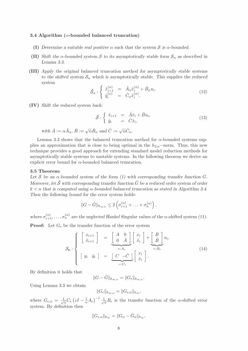
3.4 Algorithm (α-bounded balanced truncation)

(I) Determine a suitable real positive α such that the system S is α-bounded.

(II) Shift the α-bounded system S to its asymptotically stable form Sα as described inLemma 3.3.

(III) Apply the original balanced truncation method for asymptotically stable systemsto the shifted system Sα which is asymptotically stable. This supplies the reducedsystem

Sα :

{

x(α)i+1 = Aαx

(α)i + Bαui,

y(α)i = Cαx

(α)i .

(12)

(IV) Shift the reduced system back:

S :

{xi+1 = Axi + Bui,

yi = Cxi,(13)

with A := αAα, B :=√

αBα and C :=√

αCα.

Lemma 3.3 shows that the balanced truncation method for α-bounded systems sup-plies an approximation that is close to being optimal in the h2,α−norm. Thus, this newtechnique provides a good approach for extending standard model reduction methods forasymptotically stable systems to unstable systems. In the following theorem we derive anexplicit error bound for α-bounded balanced truncation.

3.5 Theorem:Let S be an α-bounded system of the form (1) with corresponding transfer function G.

Moreover, let S with corresponding transfer function G be a reduced order system of orderk < n that is computed using α-bounded balanced truncation as stated in Algorithm 3.4.Then the following bound for the error system holds:

‖G − G‖h∞,α≤ 2

(

σ(α)r+1 + . . . + σ(α)

n

)

,

where σ(α)r+1, . . . , σ

(α)n are the neglected Hankel Singular values of the α-shifted system (11).

Proof: Let Ge be the transfer function of the error system

Se :

[xi+1

xi+1

]

=

[A 0

0 A

]

︸︷︷︸

=:Ae

[xi

xi

]

+

[B

B

]

︸︷︷︸

=:Be

ui,

[yi yi

]=

[

C −C]

︸︷︷︸

=:Ce

[xi

xi

]

.

(14)

By definition it holds that‖G − G‖h∞,α

= ‖Ge‖h∞,α.

Using Lemma 3.3 we obtain‖Ge‖h∞,α

= ‖Ge,α‖h∞,

where Ge,α = 1√αCe

(zI − 1

αAe

)−1 1√αBe is the transfer function of the α-shifted error

system. By definition then

‖Ge,α‖h∞= ‖Gα − Gα‖h∞

,

8

where Gα, Gα are the transfer functions of the α-shifted systems Sα, Sα, respectively.Because the systems Sα and Sα are asymptotically stable and Sα is the result of applyingbalanced truncation to Sα the error bound (10) holds. Therefore:

‖Gα − Gα‖h∞≤ 2

(

σ(α)r+1 + . . . + σ(α)

n

)

,

where σ(α)r+1, . . . , σ

(α)n are the Hankel singular values of Gα.

Then the statement of the theorem follows with ‖Gα − Gα‖h∞= ‖G − G‖h∞,α

. �

To summarize, we state that our new technique for balanced truncation of unstablesystems computes a low order system that approximates the full order system well. It isclose to being optimal with respect to the h2,α-norm and the error in the h∞,α-norm isbounded by twice the sum of the neglected Hankel singular values of the α-shifted system.

In the following section we compare our new α-bounded balanced truncation methodwith the commonly used approach for treating unstable systems.

4 Numerical experiments

We now perform numerical experiments to illustrate the benefit of the new α-boundedmodel reduction method in comparison with the standard balanced truncation approachfor unstable systems. For these experiments we consider three different unstable discretelinear test models. In Subsections 4.1 and 4.2 the focus is on two simple discrete systemsof the form

S(k) :

{xi+1 = A(k)xi + B(k)ui,

yi = C(k)xi,for k ∈ {1, 2} (15)

with zero initial states x0 = 0. The simplicity provides a direct insight into the dynamicsof the system. A more realistic test model derived from discretized shallow water equationsis then investigated in Subsection 4.3. It is an approved test model within meteorologybecause it retains key properties of the model equations used by operational weatherforecasting centers.

4.1 First simple test model

The first test model S(1) is chosen to be a multiple-input, single-output system of the form(15), with a real diagonal matrix A(1) = diag{λ1, . . . , λ30} of dimension 30 times 30. Theinput matrix B(1) ∈ R

30×30 is the identity matrix and the output matrix C(1) ∈ R1×30 is

a row vector which contains only ones. The eigenvalues λi, i = 1 . . . 30 , of A(1) are allreal and lie inside as well as outside the unit circle. The distribution of the eigenvaluesis shown in Figure 1. We note that a considerable part of the system is unstable: 17eigenvalues lie outside the unit circle (see Appendix A.1.1 for the eigenvalues of A(1)).

We have chosen this rather simple test model because it reveals the relation betweeninputs and outputs in an obvious way. If we choose the input ui as the j-th unit impulse,i.e.

ui =

{ej for i = 0,0 for all i > 0,

where ej is the j-th canonical unit vector, then the state and the output at time ti > 0are given by

xi = λi−1j ej ,

yi = λi−1j ,

9

respectively. Thus, the impulse response yi is a power of the eigenvalue λj (the j-th di-agonal entry of the system matrix A(1)). The state vector xi only has components in thedirection of the corresponding j-th eigenvector ej .

−2 −1 0 1 2

−2.5

−2

−1.5

−1

−0.5

0

0.5

1

1.5

2

2.5

real axis

imag

inar

y ax

is

Eigenvalues of system matrix A (1)

Unit circle

Figure 1: Eigenvalues of system matrix A(1) of first simple test model

In the numerical experiments we consider a time window [t0, tN ] which consists offive to 20 time steps. Such a relatively small time window is chosen because this isthe interesting (transient) period in the case of unstable systems. In many applicationsunstable discrete systems are derived from nonlinear systems by linearization. To obtain agood approximation to the full nonlinear system it is essential to repeat the linearizationprocess every few time steps. Thus, only a small to medium size time window of thelinearized system is generally of interest.

The aim of this numerical section is to compare the new α-bounded balanced truncationapproach (proposed in Algorithm 3.4) with the standard balanced truncation methodfor unstable systems (described in Section 2). For the numerical computation of stable-unstable decompositions and of balanced realizations of asymptotically stable systems weuse the MATLAB routines stabsep.m and balreal.m, respectively, as implemented inthe Control Toolbox of MATLAB Release R2009a [13].

We now investigate the impulse responses of the full and the reduced order systemscomputed by the two different model reduction methods. Our model S(1) is a multiple-input, single-output system with 30 input channels. For such a system the impulse re-sponse at time ti is a matrix of outputs. The j-th column of this matrix contains the re-sponse of the system at time ti to an input vector that is the j-th unit impulse δj := δ(t)ej .Thus, the impulse response consists of 30 different components. For each of these we in-vestigate the approximation to the output of the full order system by the output of thelow order systems computed by standard balanced truncation and by our new α-boundedapproach.

Figure 2 shows the outputs of the first impulse response, i.e. the outputs of thesystems where the input is the first unit impulse δ1 = δ(t)e1, over the time window [t0, t5].In Figure 2(a) we see the approximation of the output of the full order system (solid line)by the output of the low order system of reduction order k = 10 computed by the standardbalanced truncation method (dashed line with circles). In comparison, Figure 2(b) showsthe output of the full order system (solid line) together with the output of the low ordersystem of reduction order k = 10 computed by the α-bounded balanced truncation method

10

for α = 12 (solid line with stars). We note that the solid line with stars is nearly invisiblein the latter case because it lies on top of the solid line. This shows that the output of theα-reduced system approximates the output of the full order system so well that the twooutput lines are indistinguishable. In contrast, the standard balanced truncation methodcomputes an output that is zero at all time steps and therefore contains no informationat all on the response of the full order system.

t_0 t_1 t_2 t_3 t_4 t_5

0

0.5

1

1.5

time

impu

lse

resp

onse

impulse response of full order systemimpulse response of standard reduced system

(a) Approximation using standard method

t_0 t_1 t_2 t_3 t_4 t_5

0

0.5

1

1.5

timeim

puls

e re

spon

se

impulse response of full order systemimpulse response of α−reduced system

(b) Approximation using α-bounded method

Figure 2: Comparison of first impulse responses of full and reduced systems of orderk = 10 using standard balanced truncation (a) as well as α-bounded balanced truncationfor α = 12.0 (b)

Figure 3 shows the corresponding error plot in logarithmic scale over the time window[t1, t5]. For illustration purposes the initial time t0 is omitted in the figure. This is reason-able because all outputs at the initial time t0 (and thus also the output errors) are zero,no matter which low order model is considered. The dashed line with circle shows theerror in the standard balanced truncation method. We see that its order of magnitude is100. In comparison the error in the α-bounded method (solid line with stars) is of orderof magnitude 10−12 to 10−15.

t_1 t_2 t_3 t_4 t_5

10−15

10−10

10−5

100

time

erro

r

error using standard methoderror using α−bounded method

Figure 3: Comparison of errors (logarithmic scale) in the first impulse response of reducedsystem of order k = 10 using standard balanced truncation (dashed line with circles) andα-bounded balanced truncation for α = 12.0 (solid line with stars)

To understand the reason that the new α-bounded method performs so much moreaccurately than the standard approach, we investigate the eigen-structure of the systemmatrices of the different low order systems. Figure 4 compares the eigenvalues of the fullorder system matrix (crosses) with those of the low order matrix computed by the standardmethod (Figure 4(a), circles) and those of the low order matrix computed by α-bounded

11

balanced truncation (Figure 4(b), circles). We see that the α-bounded approach matcheseigenvalues outside as well as inside the unit circle while the standard approach only keepssome of the eigenvalues outside the unit circle, but none inside.

Thus, the failure of the standard method is not surprising. Because of the simplestructure of this first test model we know that if the input vector ui is chosen as the firstunit impulse, then all state vectors xi are multiples of the eigenvector e1 associated withthe eigenvalue λ1 ≈ 0.8. The reduced order model computed by the standard methodneglects all directions of eigenvectors associated with asymptotically stable eigenvalues.Thus, the output of the standard low order system is not able to approximate the responseof the full order system, which is a power of the asymptotically stable eigenvalue λ1.

−2 −1 0 1 2

−2.5

−2

−1.5

−1

−0.5

0

0.5

1

1.5

2

2.5

real axis

imag

inar

y ax

is

Eigenvalues of full matrixEigenvalues of standard reducedmatrixUnit circle

(a) Eigenvalues using standard method

−2 −1 0 1 2

−2.5

−2

−1.5

−1

−0.5

0

0.5

1

1.5

2

2.5

real axis

imag

inar

y ax

is

Eigenvalues of full matrixEigenvalues of reducedα−bounded matrixUnit circle

(b) Eigenvalues using α-bounded method

Figure 4: Comparison of eigenvalues of full and reduced systems of order k = 10 usingstandard balanced truncation as well as α-bounded balanced truncation for α = 12.0

2.7 4 6 8 10 12 14 1510

−14

10−12

10−10

10−8

10−6

10−4

10−2

alpha

erro

r

h∞,α−error−norm for reduction order k=10

h∞,α−error−bound for reduction order k=10

(a) h∞,α-error-norms and -bounds

2.7 4 6 8 10 12 14 1510

−15

10−10

10−5

100

alpha

erro

r

output error for reduction order k=10

(b) Relative output errors

Figure 5: h∞,α-error-norms and -bounds and relative output errors of the impulse responseof α-bounded balanced truncation method of reduction order k = 10 for different valuesof α

As the α-bounded model reduction method is dependent on the variable α we inves-tigate the effect of the choice of α on the quality of the approximation of the low ordermodels. Figure 5 illustrates the change in the approximation error of α-bounded balancedtruncation for reduction order k = 10 for different values of α. In Figure 5(a) it is shownthat the h∞,α-error-norm ‖S(1) − S(1)‖h∞,α

(solid line) decreases with increasing α. Thedashed line is a plot of the theoretical error bound derived in Theorem 3.5. The figurevalidates the theoretical result that the actual h∞,α-error-norm (solid line) is always below

12

the error bound (dashed line). Figure 5(b) plots the behavior of the relative error normerel of the first impulse output for different values of α. The relative error norm is definedas

erel :=‖y − y‖2

‖y‖2,

where y := [y0, . . . , y5], y := [y0, . . . , y5] are the vectors of outputs of the full and the loworder systems, respectively, over the time window [t0, t5]. We see that the relative erroris smaller than 10−3 for all values of α. As α increases it even falls below 10−12. Forall values of α the approximation to the output of the first impulse response computedby α-bounded balanced truncation is much more accurate than the standard reductionapproach. However, to get a very good approximation with the α-bounded method it isrecommended to choose α not too close to the largest eigenvalue in absolute value (whichis approximately 2.63 in this test model).

t_0 t_1 t_2 t_3 t_4 t_5

0

0.5

1

1.5

time

impu

lse

resp

onse



t_0 t_1 t_2 t_3 t_4 t_5

0

0.5

1

1.5

time

impu

lse

resp

onse

impulse response of full order systemimpulse response of α−bounded reduced system


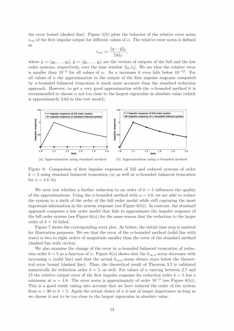
Figure 6: Comparison of first impulse responses of full and reduced systems of orderk = 5 using standard balanced truncation (a) as well as α-bounded balanced truncationfor α = 4.8 (b)

We next test whether a further reduction to an order of k = 5 influences the qualityof the approximations. Using the α-bounded method with α = 4.8, we are able to reducethe system to a sixth of the order of the full order model while still capturing the mostimportant information in the system response (see Figure 6(b)). In contrast, the standardapproach computes a low order model that fails to approximate the impulse response ofthe full order system (see Figure 6(a)) for the same reason that the reduction to the largerorder of k = 10 failed.

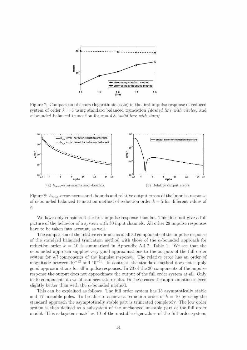
Figure 7 shows the corresponding error plot. As before, the initial time step is omittedfor illustration purposes. We see that the error of the α-bounded method (solid line withstars) is two to eight orders of magnitude smaller than the error of the standard method(dashed line with circles).

We also examine the change of the error in α-bounded balanced truncation of reduc-tion order k = 5 as a function of α. Figure 8(a) shows that the h∞,α-norm decreases withincreasing α (solid line) and that the actual h∞,α-norm always stays below the theoret-ical error bound (dashed line). Thus, the theoretical result of Theorem 3.5 is validatednumerically for reduction order k = 5, as well. For values of α varying between 2.7 and15 the relative output error of the first impulse response for reduction order k = 5 has aminimum at α = 4.8. The error norm is approximately of order 10−3 (see Figure 8(b)).This is a good result taking into account that we have reduced the order of the systemfrom n = 30 to k = 5. Again the actual choice of α is not of major importance as long aswe choose it not to be too close to the largest eigenvalue in absolute value.

13

t_1 t_2 t_3 t_4 t_5

10−5

100

time

erro

r



2.7 4 6 8 10 12 14 1510

−8

10−6

10−4

10−2

100

alpha

erro

r




2.7 4 6 8 10 12 14 1510

−3

10−2

10−1

100

alpha

erro

r



Figure 8: h∞,α-error-norms and -bounds and relative output errors of the impulse responseof α-bounded balanced truncation method of reduction order k = 5 for different values ofα

We have only considered the first impulse response thus far. This does not give a fullpicture of the behavior of a system with 30 input channels. All other 29 impulse responseshave to be taken into account, as well.

The comparison of the relative error norms of all 30 components of the impulse responseof the standard balanced truncation method with those of the α-bounded approach forreduction order k = 10 is summarized in Appendix A.1.2, Table 1. We see that theα-bounded approach supplies very good approximations to the outputs of the full ordersystem for all components of the impulse response. The relative error has an order ofmagnitude between 10−12 and 10−14. In contrast, the standard method does not supplygood approximations for all impulse responses. In 20 of the 30 components of the impulseresponse the output does not approximate the output of the full order system at all. Onlyin 10 components do we obtain accurate results. In these cases the approximation is evenslightly better than with the α-bounded method.

This can be explained as follows. The full order system has 13 asymptotically stableand 17 unstable poles. To be able to achieve a reduction order of k = 10 by using thestandard approach the asymptotically stable part is truncated completely. The low ordersystem is then defined as a subsystem of the unchanged unstable part of the full ordermodel. This subsystem matches 10 of the unstable eigenvalues of the full order system,

14

namely λ6, λ8, λ10, λ12, λ14, λ16, λ20, λ22, λ28 and λ29. Thus, whenever a component of theimpulse response stimulates one of these 10 eigenvalues, then the standard approach willsupply a low order system where the output matches the output of the full order systemexactly (assuming the absence of rounding errors), see Appendix A.1.2, Table 1. Forall remaining components of the impulse response (where none of these 10 eigenvalues isexcited) the approximation obtained by the standard approach fails. Thus, consideringthe over all comparison of the two model reduction methods (including all input channels)we see the superiority of the α-bounded approach.

Table 2 (Appendix A.1.2) shows similar results for a reduction order of k = 5. Againthe outputs of the low order system computed by the α-bounded method approximate theresponse of the full order system well for all impulse inputs. The relative output error liesbetween 10−2 and 10−5 for the responses to all unit impulse inputs. This is a good resulttaking into account that the order of the system is reduced from 30 to 5. In contrast, thestandard method only supplies good approximations for 5 out of 30 impulse responses.Again these are exactly the 5 impulse responses which excite the 5 unstable modes whichare matched by the standard method.

In these experiments we have only investigated a relatively small time window con-taining five time steps. We now conclude the investigation of the first test model S(1) bylooking at a larger window which contains 20 time steps. In Figure 9 we see the relativeerror (in logarithmic scale) in the first impulse response using the standard approach forreduction order k = 10 (dashed line with circles) and using the α-bounded method fororder k = 10 and α = 12 (solid line with stars). The α-bounded approach performs verywell for the first nine time steps with an approximation error lying between 10−5 and10−15. However, as time increases the error becomes larger, finally reaching an order ofmagnitude of 104 after 20 time steps. This reveals that the α-bounded method is espe-cially designed to capture the behavior of the system at the initial time steps. In contrast,the error of the standard method is of order of magnitude 100 for the main part of the20 time steps window becoming slightly more accurate towards the very end of the window.

t_1 t_3 t_5 t_7 t_9 t_11 t_13 t_15 t_17 t_19t_2010

−15

10−10

10−5

100

105

time

erro

r

error using standard method error using α−bounded method

Figure 9: Comparison of errors (logarithmic scale) in the first impulse response of reducedsystem of order k = 10 using standard balanced truncation (dashed line with circles) andα-bounded balanced truncation for α = 12.0 (solid line with stars) over a 20 time stepswindow

For capturing the transient motion of the system, the behavior of the reduced modelover the initial time interval is most important. For applications where the unstablelinear system is derived by linearizing a nonlinear model the first time steps are generallythe most significant and for a good approximation of the original nonlinear system thelinearization process has to be repeated every few time steps in any case. This is exactlywhere the strength of the α-bounded method lies: at the beginning of the time window thenew approach is up to 15 orders of magnitude more accurate than the standard balancedtruncation method.

We conclude the investigation of the first test model S(1) by pointing out that the

15

new α-bounded balanced truncation method supplies much better approximations to theinput-output behavior of the full order system than the standard balanced truncationapproach for unstable systems (as long as the time window is not chosen to be too large).The new method enables a reduction up to an order k = 5 while still capturing the mostimportant information for all channels of the impulse response.

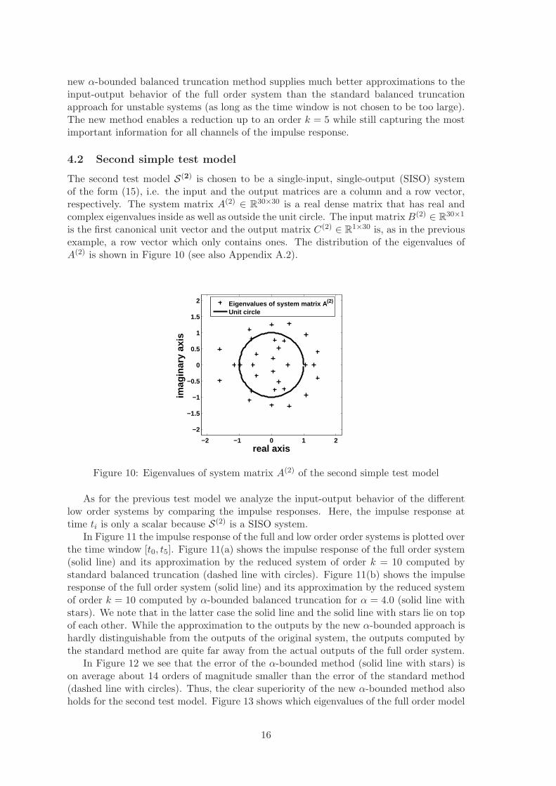
4.2 Second simple test model

The second test model S(2) is chosen to be a single-input, single-output (SISO) systemof the form (15), i.e. the input and the output matrices are a column and a row vector,respectively. The system matrix A(2) ∈ R

30×30 is a real dense matrix that has real andcomplex eigenvalues inside as well as outside the unit circle. The input matrix B(2) ∈ R

30×1

is the first canonical unit vector and the output matrix C(2) ∈ R1×30 is, as in the previous

example, a row vector which only contains ones. The distribution of the eigenvalues ofA(2) is shown in Figure 10 (see also Appendix A.2).

−2 −1 0 1 2

−2

−1.5

−1

−0.5

0

0.5

1

1.5

2

real axis

imag

inar

y ax

is

Eigenvalues of system matrix A (2)

Unit circle

Figure 10: Eigenvalues of system matrix A(2) of the second simple test model

As for the previous test model we analyze the input-output behavior of the differentlow order systems by comparing the impulse responses. Here, the impulse response attime ti is only a scalar because S(2) is a SISO system.

In Figure 11 the impulse response of the full and low order order systems is plotted overthe time window [t0, t5]. Figure 11(a) shows the impulse response of the full order system(solid line) and its approximation by the reduced system of order k = 10 computed bystandard balanced truncation (dashed line with circles). Figure 11(b) shows the impulseresponse of the full order system (solid line) and its approximation by the reduced systemof order k = 10 computed by α-bounded balanced truncation for α = 4.0 (solid line withstars). We note that in the latter case the solid line and the solid line with stars lie on topof each other. While the approximation to the outputs by the new α-bounded approach ishardly distinguishable from the outputs of the original system, the outputs computed bythe standard method are quite far away from the actual outputs of the full order system.

In Figure 12 we see that the error of the α-bounded method (solid line with stars) ison average about 14 orders of magnitude smaller than the error of the standard method(dashed line with circles). Thus, the clear superiority of the new α-bounded method alsoholds for the second test model. Figure 13 shows which eigenvalues of the full order model

16

matrix are kept by the two different model reduction techniques. The standard balancedtruncation method is capable of matching some of the eigenvalues outide the unit circle butnone inside (Figure 13(a)) while the α-bounded approach also matches (approximately) aneigenvalue inside the unit circle (Figure 13(a)). This explains why the standard methodcannot supply very accurate approximations of an output that is composed of a linearcombination of both stable and unstable modes.

t_0 t_1 t_2 t_3 t_4 t_5

−40

−30

−20

−10

0

10

20

30

time

impu

lse

resp

onse



t_0 t_1 t_2 t_3 t_4 t_5

−40

−30

−20

−10

0

10

20

30

timeim

puls

e re

spon

se



Figure 11: Comparison of impulse responses of full and reduced systems of order k = 10using standard balanced truncation (a) as well as α-bounded balanced truncation forα = 4.0 (b)

t_1 t_2 t_3 t_4 t_5

10−15

10−10

10−5

100

105

time

erro

r



We also examine the effect of different choices of α on the error norms of the low orderapproximations. Figure 14(a) illustrates that the actual h∞,α-norm of the error system(solid line) is always smaller than the computed theoretical error bound (dashed line). InFigure 14(b) we see a plot of the relative error erel of the impulse response for differentvalues of α. As long as α is chosen to be not too close to the largest eigenvalue of thesystem matrix in absolute value (which is approximately 1.68), then the output error erel

becomes very small. For α > 3.5 it even has the order of magnitude of the machineprecision.

As for the first test model S(1), we now investigate whether a further order reduction ofthe low order model is possible. We find that, using the α-bounded approach, a reductionup to a sixth of the order of the original system still supplies a good approximation.The most essential information of the input-output behavior is retained. Computing alow order system of order k = 5 using the α-bounded method, we obtain outputs that

17

accurately approximate the outputs of the full order systems (see Figures 14(c), 14(d)).We note again that the actual choice of α is not significant as long as it is not too closeto the largest eigenvalue in absolute value.

−2 −1 0 1 2

−2

−1

0

1

2

real axis

imag

inar

y ax

is

Eigenvalues of full matrixEigenvalues of standard reducedmatrixUnit circle

(a) Eigenvalues using standard method

−2 −1 0 1 2

−2

−1

0

1

2

real axis

imag

inar

y ax

is

Eigenvalues of full matrixEigenvalues of reduced α−boundedmatrixUnit circle

(b) Eigenvalues using α-bounded method

Figure 13: Comparison of eigenvalues of full and reduced systems of order k = 10

2 2.5 3 3.5 4 4.5 5 5.5 61.710

−15

10−10

10−5

100

alpha

erro

r




2 2.5 3 3.5 4 4.5 5 5.5 61.710

−15

10−10

10−5

100

alpha

erro

r



4 6 8 10 12 141.7 1510

−10

10−5

100

105

alpha

erro

r



(c) h∞,α-error-norms and -bounds

4 6 8 10 12 14 151.710

−15

10−10

10−5

100

alpha

erro

r


(d) Relative output errors

Figure 14: h∞,α-error-norms and -bounds and relative errors of impulse response of α-bounded balanced truncation method of reduction order k = 10, k = 5 for different α

4.3 Shallow water model

In addition to the two simple models we investigate, as a third test model S(3), a 1-dimensional shallow water system which describes the flow of a fluid over an obstacle with

18

rotation. The corresponding continuous shallow water equations are given by

Du

Dt+

∂φ

∂x+ g

∂H

∂x− fv = 0,

Dv

Dt+ fu = 0,

D ln φ

Dt+

∂u

∂x= 0,

whereD

Dt≡ ∂

∂t+ (Uc + u)

∂

∂x

andφ = gh,

where u denotes the departure of the velocity in the x-direction from a known constantforcing mean flow Uc, H = H(x) is the height of the orography, f is the Coriolis parameterand g is the gravitational force. The model assumes that velocities u and v as well as thedepth h do not vary in the y-direction. Moreover, the model states are periodic in thex-direction. The continuous equations are discretized using a two-time-level semi-implicitsemi-Lagrangian integration scheme, following [11]. The discrete nonlinear system is thenlinearized by computing the Jacobian of the nonlinear system equations. The resultingdiscrete linear system is known as the tangent linear model.

A time-invariant linear model that approximates the tangent linear model of the systemis used in the experiments. It is a multiple-input, multiple-output (MIMO) system. Itssystem matrix A(3) and its input matrix B(3) are both of dimension 1500 × 1500. Theoutput matrix C(3) ∈ R

750×1500 is chosen such that every other point is observed. We referto the first, second and third set of 500 components of the state vector as the u-, v- andφ-field, respectively.

This test model is only slightly unstable, i.e. only 10 of the 1500 eigenvalues lie strictlyoutside the unit circle and the absolute value of the largest eigenvalue is approximately1.00013 (see Figure 15 for the distribution of the eigenvalues). However, the system is stillan interesting test model because many of the asymptotically stable poles are so close tobeing unstable that it is impossible to separate them properly from the unstable poles.

We now investigate whether similar results to those for the two simple systems continueto hold for the shallow water test model S(3). This is a discrete MIMO system of order 1500with 1500 input and 750 output channels. Obviously, it is not possible to consider all 1500components of the impulse response. In the following we focus only on one representativecomponent of the impluse response, its 250th, at time t = t5.

Figure 16 shows the u-field vector components of the 250th impulse response after fivetime steps. The top figure (16(a)) contains a comparison of the impulse response of thefull order system (solid line) and the low order system computed by standard balancedtruncation of reduction order k = 750 (dashed line with circles). We see that the low ordermodel does not approximate the full order system accurately. In contrast, Figure 16(b)shows the approximation to the full order impulse response (solid line) by the low orderapproximation using α-bounded balanced truncation of order k = 750 for α = 1.1 (solidline with stars). Here the solid line and the solid line with stars lie on top of each otherwhich shows the excellent performance of the α-bounded approach. The correspondingerror (in logarithmic scale) is visualized in Figure 16(c). We see that the approximationerror of the α-bounded method (solid line with stars) is of order 10−6 on average. Thisis three orders of magnitude smaller than the error of the standard method (dashed linewith circles).

19

Very similar results hold for the φ-field vector components of the 250th impulse re-sponse as shown in Figure 17. The error of the α-bounded approach (solid line with stars)is approximately two orders of magnitude smaller than the error of the standard method(dashed line with circles). We omit to show the analog figure for the v-field where thetrue solution is almost zero everywhere. The errors in the standard and the α-boundedmethod are of the same orders of magnitude as for the u- and the φ-field.

−1 −0.5 0 0.5 1

−1

−0.8

−0.6

−0.4

−0.2

0

0.2

0.4

0.6

0.8

1

real axis

imag

inar

y ax

is

Figure 15: Eigenvalues of system matrix A(3) of the shallow water test model

We now investigate the effect of a further reduction to an order of k = 150, a tenthof the order of the full system. Figures 18 and 19 show the u- and the φ-field vectorcomponents of the 250th impulse response for k = 150 after five time steps, respectively.Despite the large reduction, the approximation error of the α-bounded method is still, onaverage, of order 10−4 (solid line with stars). This is two orders of magnitude smaller thanthe error of the standard method (dashed line with circles).

For the first test model S(1) we observed that the performance of the α-boundedmethod becomes quite poor when the time window consists of more than ten steps (seeFigure 9). Figure 20 shows that this does not hold for the shallow water test model. After20 time steps the errors in the u-,v- and φ-field components of the 250th impulse responseof the α-bounded method for α = 1.1 and order k = 750 (solid line with stars) are still onaverage two to three orders of magnitude smaller than the errors of the standard approachfor order k = 750 (dashed line with circles).

20

0 50 100 150 200 250−0.01

−0.005

0

0.005

0.01

0.015

0.02

0.025

vector components

impu

lse

resp

onse

impulse response of full order systemimpulse response ofstandard reduced system

(a) u-field approximation using standard balanced truncation

0 50 100 150 200 250−0.005

0

0.005

0.01

0.015

0.02

0.025

vector components

impu

lse

resp

onse


(b) u-field approximation using α-bounded balanced truncation

0 50 100 150 200 25010

−8

10−7

10−6

10−5

10−4

10−3

10−2

10−1

vector components

erro

r


(c) Errors in u-field approximations

Figure 16: Comparison of u-field vector components of 250th impulse response of fulland reduced systems of order k = 750 using standard balanced truncation (a) as well asα-bounded balanced truncation for α = 1.1 (b) after five time steps. Subfigure (c) showsthe corresponding error plot in logarithmic scale.

21

0 50 100 150 200 250−0.5

−0.4

−0.3

−0.2

−0.1

0

0.1

0.2

0.3

0.4

0.5

vector components

impu

lse

resp

onse


(a) φ-field approximation using standard balanced truncation

0 50 100 150 200 250−0.5

−0.4

−0.3

−0.2

−0.1

0

0.1

0.2

0.3

0.4

0.5

vector components

impu

lse

resp

onse


(b) φ-field approximation using α-bounded balanced truncation

0 50 100 150 200 25010

−8

10−6

10−4

10−2

100

vector components

erro

r


(c) Errors in φ-field approximations

Figure 17: Comparison of φ-field vector components of 250th impulse response of fulland reduced systems of order k = 750 using standard balanced truncation (a) as well asα-bounded balanced truncation for α = 1.1 (b) after five time steps. Subfigure (c) showsthe corresponding error plot in logarithmic scale.

22

0 50 100 150 200 250−0.01

−0.005

0

0.005

0.01

0.015

0.02

0.025

vector components

impu

lse

resp

onse

impulse response of full order systemimpulse response ofstandard reduced system

(a) u-field approximation using standard balanced truncation

0 50 100 150 200 250−0.005

0

0.005

0.01

0.015

0.02

0.025

vector components

impu

lse

resp

onse

impulse response of full order systemimpulse response ofα−bounded reduced system

(b) u-field approximation using α-bounded balanced truncation

0 50 100 150 200 25010

−8

10−6

10−4

10−2

100

vector components

erro

r


(c) Errors in u-field approximations

Figure 18: Comparison of u-field vector components of 250th impulse response of fulland reduced systems of order k = 150 using standard balanced truncation (a) as well asα-bounded balanced truncation for α = 1.1 (b) after five time steps. Subfigure (c) showsthe corresponding error plot in logarithmic scale.

23

0 50 100 150 200 250−0.5

−0.4

−0.3

−0.2

−0.1

0

0.1

0.2

0.3

0.4

0.5

vector components

impu

lse

resp

onse


(a) φ-field approximation using standard balanced truncation

0 50 100 150 200 250−0.5

−0.4

−0.3

−0.2

−0.1

0

0.1

0.2

0.3

0.4

0.5

vector components

impu

lse

resp

onse


(b) φ-field approximation using α-bounded balanced truncation

0 50 100 150 200 25010

−5

10−4

10−3

10−2

10−1

100

vector components

erro

r


(c) Errors in φ-field approximations

Figure 19: Comparison of φ-field vector components of 250th impulse response of fulland reduced systems of order k = 150 using standard balanced truncation (a) as well asα-bounded balanced truncation for α = 1.1 (b) after five time steps. Subfigure (c) showsthe corresponding error plot in logarithmic scale.

24

0 50 100 150 200 25010

−8

10−7

10−6

10−5

10−4

10−3

10−2

10−1

vector components

erro

r


(a) u-field vector components

0 50 100 150 200 25010

−12

10−10

10−8

10−6

10−4

10−2

100

vector components

erro

r

error using standard method of order k = 750error using α−bounded method of order k = 750 and α = 1.1

(b) v-field vector components

0 50 100 150 200 25010

−10

10−8

10−6

10−4

10−2

100

vector components

erro

r


(c) φ-field vector components

Figure 20: Comparison of errors in u-, v- and φ-field vector components of 250th impulseresponse of full and reduced system of order k = 750 using standard balanced truncation(dashed line with circles) and α-bounded balanced truncation for α = 1.1 (solid line withstars) after 20 time steps.

25

4.4 Summary of numerical experiments

All the numerical experiments demonstrated the superiority of the α-bounded balancedtruncation method over the currently used balanced truncation approach for unstable sys-tems, especially over a short time window. This result is not very surprising. If the systemhas a considerable number of unstable poles, then the standard approach for unstable sys-tems cannot supply a good approximation to the input-output behavior of the full ordersystem. The reason is that essential or even all information of the asymptotically stablepart of the full order system is lost (depending on the chosen reduction order). Thus,at the beginning of the time window (where the asymptotically stable part still influ-ences the behavior of the system) we cannot expect the standard approach to supply goodapproximations.

Moreover, the shallow water test model showed that the standard balanced truncationmethod fails not only for systems with large numbers of unstable poles, but also for systemsthat have only a few unstable poles, but large numbers of asymptotically stable modesthat are very close to being unstable.

5 Conclusions

Model order reduction of unstable control systems is an important problem to be consid-ered. However, most of the known and approved model reduction methods are for asymp-totically stable systems only. The existing approaches for unstable systems are based onan additive decomposition of the system into its asymptotically stable and its unstablepart. The model reduction procedure is then applied to the asymptotically stable subsys-tem while the unstable part remains unchanged. This procedure may only supply goodapproximations to the full order system if the number of unstable poles is rather small orif the asymptotically stable part of the system is of minor importance. These assumptionsare rather restrictive. At the beginning of the time window, especially, the standard loworder approximations are poor because at the initial time steps the asymptotically stablecomponents (which are neglected in the standard approach) still have influence on thebehavior of the system.

In this paper we have proposed a novel approach for model reduction for unstablesystems using balanced truncation. The new α-bounded balanced truncation method isindependent of the number of unstable poles. It equally takes into account the asymptot-ically stable as well as the unstable modes of the full order system within the reductionprocess. We were able to show that the new method is embedded in a theoretical frameworkvery similar to that of the original balanced truncation method for asymptotically stablesystems. While balanced truncation for asymptotically stable systems computes a loworder system that is close to being optimal with respect to the h2-norm, the α-boundedbalanced truncation method supplies a low order system close to being optimal in theh2,α-norm. Moreover, we have proved a theoretical error bound for the new α-boundedapproach based on neglected Hankel singular values.

In numerical experiments with two simple unstable test models we have shown thatthe new method computes a low order model that approximates the input-output behaviorof the full order system very accurately. It is possible even to reduce the order up to asixth of the order of the original system while still capturing the essential information inthe response. Comparison with the standard balanced truncation approach for unstablesystems demonstrated the superiority of the new α-bounded balanced truncation method,especially at the beginning of the time window.

In addition to the simple models, we have also investigated a more realistic test model

26

derived from discretized and linearized shallow water equations. This model has only asmall number of unstable poles and the largest unstable eigenvalue is only slightly largerthan unity. At first sight this situation suggests that the standard approach should workwell. However, this is not the case. Here the failure of the standard approach is causedby a large number of asymptotically stable poles which are so close to being unstablethat it is impossible to separate them properly in the stable-unstable decomposition. Thenumerical experiments again showed the superiority of the new α-bounded method. Fora reduction order of 150 which is a tenth of the order of the original system the error ofthe α-bounded method is still, on average, of order of magnitude 10−4. This is two ordersof magnitude smaller than the error in the standard approach.

27

A Appendix

A.1 First test model S(1)

A.1.1 Eigenvalues of first test model

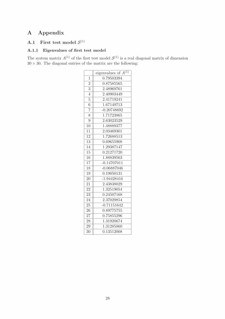
The system matrix A(1) of the first test model S(1) is a real diagonal matrix of dimension30 × 30. The diagonal entries of the matrix are the following:

eigenvalues of A(1)

1 0.79503394

2 0.87585565

3 2.48969761

4 2.40903449

5 2.41719241

6 1.67149713

7 -0.20748692

8 1.71723865

9 2.63023529

10 1.48889377

11 2.03469301

12 1.72688513

13 0.69655908

14 1.29387147

15 0.21271720

16 1.88839563

17 -0.14707011

18 -0.06887046

19 0.19050131

20 -1.94428416

21 2.43838029

22 1.32519054

23 0.24507168

24 2.37029854

25 -0.71151642

26 0.89775755

27 0.75855296

28 1.31920674

29 1.31285860

30 0.13512008

28

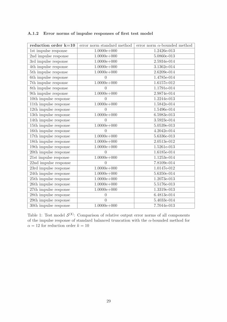
A.1.2 Error norms of impulse responses of first test model

reduction order k=10 error norm standard method error norm α-bounded method

1st impulse response 1.0000e+000 1.2426e-013

2nd impulse response 1.0000e+000 5.0860e-013

3rd impulse response 1.0000e+000 2.5934e-014

4th impulse response 1.0000e+000 3.1362e-014


6th impulse response 0 1.4785e-014
















22nd impulse response 0 7.8109e-014









Table 1: Test model S(1): Comparison of relative output error norms of all componentsof the impulse response of standard balanced truncation with the α-bounded method forα = 12 for reduction order k = 10

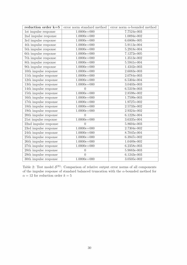
29

reduction order k=5 error norm standard method error norm α-bounded method


2nd impulse response 1.0000e+000 1.0094e-002




















22nd impulse response 0 5.8604e-003









Table 2: Test model S(1): Comparison of relative output error norms of all componentsof the impulse response of standard balanced truncation with the α-bounded method forα = 12 for reduction order k = 5

30

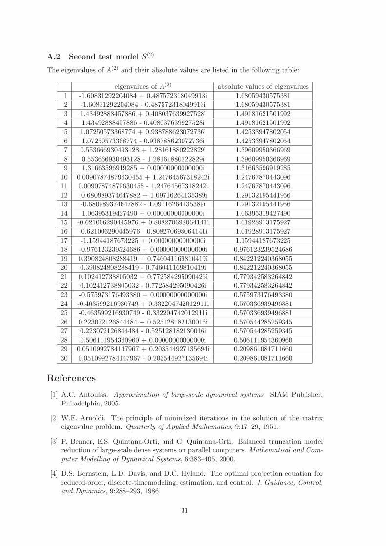
A.2 Second test model S(2)

The eigenvalues of A(2) and their absolute values are listed in the following table:

eigenvalues of A(2) absolute values of eigenvalues

1 -1.60831292204084 + 0.487572318049913i 1.68059430575381

2 -1.60831292204084 - 0.487572318049913i 1.68059430575381

3 1.43492888457886 + 0.408037639927528i 1.49181621501992

4 1.43492888457886 - 0.408037639927528i 1.49181621501992

5 1.07250573368774 + 0.938788623072736i 1.42533947802054

6 1.07250573368774 - 0.938788623072736i 1.42533947802054

7 0.553666930493128 + 1.28161880222829i 1.39609950366969

8 0.553666930493128 - 1.28161880222829i 1.39609950366969

9 1.31663596919285 + 0.00000000000000i 1.31663596919285

10 0.00907874879630455 + 1.24764567318242i 1.24767870443096

11 0.00907874879630455 - 1.24764567318242i 1.24767870443096

12 -0.680989374647882 + 1.09716264135389i 1.29132195441956

13 -0.680989374647882 - 1.09716264135389i 1.29132195441956

14 1.06395319427490 + 0.00000000000000i 1.06395319427490

15 -0.621006290445976 + 0.808270698064141i 1.01928913175927

16 -0.621006290445976 - 0.808270698064141i 1.01928913175927

17 -1.15944187673225 + 0.00000000000000i 1.15944187673225

18 -0.976123239524686 + 0.00000000000000i 0.976123239524686

19 0.390824808288419 + 0.746041169810419i 0.842212240368055

20 0.390824808288419 - 0.746041169810419i 0.842212240368055

21 0.102412738805032 + 0.772584295090426i 0.779342583264842

22 0.102412738805032 - 0.772584295090426i 0.779342583264842

23 -0.575973176493380 + 0.00000000000000i 0.575973176493380

24 -0.463599216930749 + 0.332204742012911i 0.570336939496881

25 -0.463599216930749 - 0.332204742012911i 0.570336939496881

26 0.223072126844484 + 0.525128182130016i 0.570544285259345

27 0.223072126844484 - 0.525128182130016i 0.570544285259345

28 0.506111954360960 + 0.00000000000000i 0.506111954360960

29 0.0510992784147967 + 0.203544927135694i 0.209861081711660

30 0.0510992784147967 - 0.203544927135694i 0.209861081711660

References

[1] A.C. Antoulas. Approximation of large-scale dynamical systems. SIAM Publisher,Philadelphia, 2005.

[2] W.E. Arnoldi. The principle of minimized iterations in the solution of the matrixeigenvalue problem. Quarterly of Applied Mathematics, 9:17–29, 1951.

[3] P. Benner, E.S. Quintana-Orti, and G. Quintana-Orti. Balanced truncation modelreduction of large-scale dense systems on parallel computers. Mathematical and Com-puter Modelling of Dynamical Systems, 6:383–405, 2000.

[4] D.S. Bernstein, L.D. Davis, and D.C. Hyland. The optimal projection equation forreduced-order, discrete-timemodeling, estimation, and control. J. Guidance, Control,and Dynamics, 9:288–293, 1986.

31

[5] C. Boess. Using model reduction techniques within the incremental 4D-Var method.PhD thesis, Universitaet Bremen, 2008.

[6] S. Gerschgorin. ber die abgrenzung der eigenwerte einer matrix. Izv. Akad. Nauk.USSR Otd. Fiz.-Mat. Nauk, 7:749–754, 1993.

[7] K. Glover. All optimal hankel norm approximation of linear multivariable systemsand their L∞ error bounds. Int. J. Contr., 39:1115–1193, 1984.

[8] G.H. Golub and C.F. van Loan. Matrix computations. Johns Hopkins UniversityPress, Baltimore, third edition, 1996.

[9] D. Hinrichsen and A.J. Pritchard. Mathematical Systems Theory I. Springer, Berlin,2005.

[10] C.S. Hsu and D. Hou. Reducing unstable linear control systems via real schur trans-formation. Electron. Lett., pages 984–986, 1991.

[11] D. Katz, A.S. Lawless, N.K. Nichols, M.J.P. Cullen, and R.N. Bannister. A com-parison of potential vorticity-based and vorticity-based control variables. NumericalAnalysis Report, 8/2005.

[12] D. Kubalinska. Optimal interpolation-based model reduction. PhD thesis, UniversitaetBremen, 2008.

[13] MATLAB. Control Toolbox. The MathWorks, Release R2009a.

[14] B.C. Moore. Principal component analysis in linear systems:controllability, observ-ability and model reduction. IEEE Trans. Automatic Control, 26:17–32, 1981.

[15] S.K. Nagar and S.K. Singh. An algorithmic approach for system dedcomposition andbalanced realized model reduction. J. of Franklin Inst., 341:615–630, 2004.

[16] L. Pernebo and L.M. Silverman. Model reduction via balanced state space represen-tations. IEEE Trans. Automatic Control, 27:382–387, 1982.

[17] Y. Saad. Numerical Methods for Large Eigenvalue Problems. Manchester UniversityPress, 1992.

[18] A. Varga. Balancing-free square-root algorithm for computing singular pertubationapproximations. Proc. 30th IEEE CDC, Brighton, pages 1062–1065, 1991.

[19] A. Varga. Model reduction software in the slicot library. Applied and ComputationalControl, Signals and Circuits, 629:239–282, 2001.

32

model order reduction for discrete unstable control ... order reduction for discrete unstable...

Documents