model integration in data mining: from local to global...

Universitat Politecnica de Valencia

Departamento de Sistemas Informaticos y Computacion

Doctorado en Informatica

Ph.D. Thesis

Model Integration in Data Mining:From Local to Global Decisions

Candidate:

Antonio Bella Sanjuan

Supervisors:

Cesar Ferri Ramırez,Jose Hernandez Orallo andMarıa Jose Ramırez Quintana.

– June 2012 –

This work has been partially supported by the EU (FEDER) and the SpanishMICINN, under grants TIN2010-21062-C02-02, TIN2007-68093-C02-02; theGeneralitat Valenciana under grant GV06/301 and project PROMETEO/2008/051;the UPV under grant TAMAT; and the Spanish project “Agreement Technolo-gies” (Consolider Ingenio CSD2007-00022).

Author’s address:

Departamento de Sistemas Informaticos y ComputacionUniversitat Politecnica de ValenciaCamino de Vera, s/n46022 ValenciaEspana

A mis padres.A mis hermanas.

A Marıa.

Acknowledgments

Echo la vista atras y me acuerdo de aquel primer dıa en que empece mi carreraen la UPV. Recuerdo que pense: “al menos durante los 5 proximos anostendre que hacer este mismo recorrido todos los dıas”. Y ası fue, pero lo queno pensaba es que despues de la ingenierıa vendrıa el doctorado, ası que heseguido haciendo ese mismo camino, pero en coche en vez de en tranvıa.

Esta tesis, que tiene entre sus manos, en la pantalla de su ordenador odispositivo movil, es la culminacion de todos estos anos de investigacion conun grupo de personas con las que muchas veces he compartido mas tiempoque con mi familia y a los que les doy las gracias. Con ellos he compartidoesos momentos de frustracion en los que no sale nada y en los que lo masfacil serıa abandonar, pero siempre me han apoyado para seguir adelante. Y,por supuesto, tambien hemos compartido los buenos momentos de alegrıa ysatisfaccion, que al final son los que mas se recuerdan. Todo esto para decirlesque si no fuese por ellos no estarıan leyendo lo que estan leyendo.

En particular, gracias a Salvador Lucas que empezo toda esta aventuraenviandome un correo para una beca. A Marıa Alpuente, lıder del grupo ELP,que me dio la oportunidad de pertenecer a este grupo. A mis directores detesis: Jose, Marıa Jose y Cesar, por toda la ayuda que me han brindado y porsu paciencia y dedicacion en las revisiones de los trabajos que hemos realizadojuntos. A Bea por todo el tiempo que hemos compartido juntos, por todo loque hemos llorado y sobre todo por todo lo que hemos reıdo. A Vicent portodos sus buenos consejos. A Josep por su “introduccion a la investigacion”.A Raquel por nuestras charlas. A Tama, Sonia, Rafa, Michele y Vesna porquelas comidas de esa epoca llegaron a ser el momento mas divertido del dıa. Ya todos los companeros que han pasado por el grupo ELP durante estos anosy que no enumero porque prefiero no olvidarme de ninguno.

Y en especial, muchas gracias a mis padres, a mis hermanas y a mi noviaMarıa que saben todo lo que ha costado llegar hasta este momento y que apartir de hoy van a estar un poco mas orgullosos de su hijo/hermano/novio.

No se que me deparara el futuro, eso solo el tiempo lo dira, pero de loque estoy seguro es que estarıa encantado de seguir recorriendo cada dıa estemismo camino.

Junio 2012,Antonio Bella.

Abstract

Machine Learning is a research area that provides algorithms and techniquesthat are capable of learning automatically from past experience. These tech-niques are essential in the area of Knowledge Discovery from Databases (KDD),whose central stage is typically referred to as Data Mining. The KDD processcan be seen as the learning of a model from previous data (model generation)and the application of this model to new data (model deployment). Model de-ployment is very important, because people and, very especially, organisationsmake decisions depending on the results of the models.

Usually, each model is learned independently from the others, trying toobtain the best (local) result. However, when several models have to be usedtogether, some of them can depend on each other (e.g., outputs of a model areinputs of other models) and constraints appear on their application. In thisscenario, the best local decision for each individual problem could not givethe best global result, or the result could be invalid if it does not fulfill theproblem constraints.

Customer Relationship Management (CRM) is an area that has originatedreal application problems where data mining and (global) optimisation need tobe combined. For example, prescription problems deal about distinguishing orranking the products to be offered to each customer (or simetrically, selectingthe customers to whom we should make an offer). These areas (KDD, CRM)are lacking tools for a more holistic view of the problems and a better modelintegration according to their interdependencies and the global and local con-straints. The classical application of data mining to prescription problems hasusually considered a rather monolitic and static view of the process, wherewe have one or more products to be offered to a pool of customers, and weneed to determine a sequence of offers (product, customer) to maximise profit.We consider that it is possible to perform a better customisation by tuning oradapting several features of the product to get more earnings. Therefore, wepresent a taxonomy of prescription problems based on the presence or absenceof special features that we call negotiable features. We propose a solution foreach kind of problem, based on global optimisation (combining several modelsin the deployment phase) and negotiation (introducing new concepts, prob-lems and techniques). In general, in this scenario, obtaining the best globalsolution analytically is unreachable and simulation techniques are useful in

order to obtain good global results.Furthermore, when several models are combined, they must be combined

using an unbiased criterion. In the case of having an estimated probability foreach example, these probabilities must be realistic. In machine learning, thedegree to which estimated probabilities match the actual probabilities is knownas calibration. We revisit the problem of classifier calibration, proposing a newnon-monotonic calibration method inspired in binning-based methods. More-over, we study the role of calibration before and after probabilistic classifiercombination. We present a series of findings that allow us to recommendseveral layouts for the use of calibration in classifier combination.

Finally, before deploying the model, making single decisions for each newindividual, a global view of the problem may be required, in order to study thefeasibility of the model or the resources that will be needed. Quantification is amachine learning task that can help to obtain this global view of the problem.We present a new approach to quantification based on scaling the averageestimated probability. We also analyse the impact of having good probabilityestimators for the new quantification methods based on probability average,and the relation of quantification with global calibration.

Summarising, in this work, we have developed new techniques, methodsand algorithms that can be applied during the model deployment phase fora better model integration. These new contributions outperform previousapproaches, or cover areas that have not already been studied by the machinelearning community. As a result, we now have a wider and more powerfulrange of tools for obtaining good global results when several local models arecombined.

Keywords: classifier combination, global optimisation, negotiable features,simulation, calibration, quantification.

Resumen

El aprendizaje automatico es un area de investigacion que proporciona al-goritmos y tecnicas que son capaces de aprender automaticamente a partirde experiencias pasadas. Estas tecnicas son esenciales en el area de descu-brimiento de conocimiento de bases de datos (KDD), cuya fase principal estıpicamente conocida como minerıa de datos. El proceso de KDD se puede vercomo el aprendizaje de un modelo a partir de datos anteriores (generacion delmodelo) y la aplicacion de este modelo a nuevos datos (utilizacion del modelo).La fase de utilizacion del modelo es muy importante, porque los usuarios y,muy especialmente, las organizaciones toman las decisiones dependiendo delresultado de los modelos.

Por lo general, cada modelo se aprende de forma independiente, intentandoobtener el mejor resultado (local). Sin embargo, cuando varios modelos se usanconjuntamente, algunos de ellos pueden depender los unos de los otros (porejemplo, las salidas de un modelo pueden ser las entradas de otro) y aparecenrestricciones. En este escenario, la mejor decision local para cada problematratado individualmente podrıa no dar el mejor resultado global, o el resultadoobtenido podrıa no ser valido si no cumple las restricciones del problema.

El area de administracion de la relacion con los clientes (CRM) ha dadoorigen a problemas reales donde la minerıa de datos y la optimizacion (global)deben ser usadas conjuntamente. Por ejemplo, los problemas de prescripcionde productos tratan de distinguir u ordenar los productos que seran ofrecidosa cada cliente (o simetricamente, elegir los clientes a los que se les deberıa deofrecer los productos). Estas areas (KDD, CRM) carecen de herramientas paratener una vision mas completa de los problemas y una mejor integracion delos modelos de acuerdo a sus interdependencias y las restricciones globales ylocales. La aplicacion clasica de minerıa de datos a problemas de prescripcionde productos, por lo general, ha considerado una vision monolıtica o estaticadel proceso, donde uno o mas productos son ofrecidos a un conjunto de clien-tes y se tiene que determinar la secuencia de ofertas (producto, cliente) quemaximice el beneficio. Consideramos que es posible realizar una mejor perso-nalizacion del proceso ajustando o adaptando varios atributos del productopara obtener mayores ganancias. Por lo tanto, presentamos una taxonomıade problemas de prescripcion de productos basada en la presencia o ausenciade un tipo de atributos especiales que llamamos atributos negociables. Pro-

ponemos una solucion para cada tipo de problema, basada en optimizacionglobal (combinando varios modelos en la fase de utilizacion de los modelos)y negociacion (introduciendo nuevos conceptos, problemas y tecnicas). En ge-neral, en este escenario, obtener la mejor solucion global de forma analıticaes intratable y usar tecnicas de simulacion es una manera de obtener buenosresultados a nivel global.

Ademas, cuando se combinan varios modelos, estos tienen que combinarseusando un criterio justo. Si para cada ejemplo tenemos su probabilidad es-timada, esta probabilidad tiene que ser realista. En aprendizaje automatico,el grado en el que las probabilidades estimadas se corresponden con las pro-babilidades reales se conoce como calibracion. Retomamos el problema de lacalibracion de clasificadores, proponiendo un metodo de calibracion no mo-notonico inspirado en los metodos basados en “binning”. Por otra parte, es-tudiamos el papel de la calibracion antes y despues de combinar clasificadoresprobabilısticos. Y presentamos una serie de conclusiones que nos permiten re-comendar varias configuraciones para el uso de la calibracion en la combinacionde clasificadores.

Por ultimo, antes de usar el modelo, tomando decisiones individuales pa-ra cada nuevo ejemplo, puede ser necesaria una vision global del problema,para estudiar la viabilidad del modelo o los recursos que seran necesarios. Lacuantificacion es una tarea de aprendizaje automatico que puede ayudar a ob-tener esta vision global del problema. Presentamos una nueva aproximacional problema de cuantificacion basada en escalar la media de la probabilidadestimada. Tambien se analiza el impacto de tener un buen estimador de pro-babilidades para estos nuevos metodos de cuantificacion, y la relacion de lacuantificacion con la calibracion global.

En resumen, en este trabajo, hemos desarrollado nuevas tecnicas, metodosy algoritmos que se pueden aplicar durante la fase de utilizacion de los mo-delos para una mejor integracion de estos. Las nuevas contribuciones mejoranlas aproximaciones anteriores, o cubren areas que aun no habıan sido estu-diadas por la comunidad de aprendizaje automatico. Como resultado, ahoratenemos una gama mas amplia y potente de herramientas para obtener buenosresultados globales cuando combinamos varios modelos locales.

Palabras clave: combinacion de clasificadores, optimizacion global, atri-butos negociables, simulacion, calibracion, cuantificacion.

Resum

L’aprenentatge automatic es una area d’investigacio que proporciona algorit-mes i tecniques que son capacos d’aprendre automaticament a partir d’expe-riencies passades. Estes tecniques son essencials en l’area de descobriment deconeixement de bases de dades (KDD), la fase principal de la qual es tıpicamentconeguda com a mineria de dades. El proces de KDD es pot veure com l’a-prenentatge d’un model a partir de dades anteriors (generacio del model) il’aplicacio d’este model a noves dades (utilitzacio del model). La fase d’uti-litzacio del model es molt important, perque els usuaris i, molt especialment,les organitzacions prenen les decisions depenent del resultat dels models.

Generalment, cada model s’apren de forma independent, intentant obtin-dre el millor resultat (local). No obstant aixo, quan diversos models s’usenconjuntament, alguns d’ells poden dependre els uns dels altres (per exemple,les eixides d’un model poden ser les entrades d’un altre) i apareixen restric-cions. En aquest escenari, la millor decisio local per a cada problema tractatindividualment podria no donar el millor resultat global, o el resultat obtingutpodria no ser valid si no complix les restriccions del problema.

L’area d’administracio de la relacio amb els clients (CRM) ha donat origena problemes reals on la mineria de dades i l’optimitzacio (global) han de serusades conjuntament. Per exemple, els problemes de prescripcio de productestracten de distingir o ordenar els productes que seran oferits a cada client (osimetricament, triar els clients a qui se’ls deuria d’oferir els productes). Estesarees (KDD, CRM) no tenen ferramentes per a tindre una visio mes comple-ta dels problemes i una millor integracio dels models d’acord amb les seuesinterdependencies i les restriccions globals i locals. Generalment, l’aplicacioclassica de mineria de dades a problemes de prescripcio de productes ha con-siderat una visio monolıtica o estatica del proces, on un o mes productes sonoferits a un conjunt de clients i s’ha de determinar la sequencia d’ofertes (pro-ducte, client) que maximitze el benefici. Considerem que es possible realitzaruna millor personalitzacio del proces ajustant o adaptant diversos atributs delproducte per a obtindre majors guanys. Per tant, presentem una taxonomia deproblemes de prescripcio de productes basada en la presencia o absencia d’untipus d’atributs especials que cridem atributs negociables. Proposem una so-lucio per a cada tipus de problema, basada en optimitzacio global (combinantdiversos models en la fase d’utilitzacio) i negociacio (introduint nous concep-

tes, problemes i tecniques). En general, en aquest escenari, obtindre la millorsolucio global de forma analıtica es intractable i usar tecniques de simulacioes una manera d’obtindre bons resultats a nivell global.

A mes, quan es combinen diversos models, estos han de combinar-se usantun criteri just. Si per a cada exemple tenim la seua probabilitat estimada, estaprobabilitat ha de ser realista. En aprenentatge automatic, el grau en que lesprobabilitats estimades es corresponen amb les probabilitats reals es coneixcom a calibracio. Reprenem el problema de la calibracio de classificadors,proposant un metode de calibracio no monotonic inspirat en els metodes basatsen “binning”. D’altra banda, estudiem el paper de la calibracio abans i despresde combinar classificadors probabilıstics. I presentem una serie de conclusionsque ens permeten recomanar diverses configuracions per a l’us de la calibracioen la combinacio de classificadors.

Finalment, abans d’usar el model, prenent decisions individuals per a cadanou exemple, pot ser necessaria una visio global del problema, per a estudiar laviabilitat del model o els recursos que seran necessaris. La quantificacio es unatasca d’aprenentatge automatic que pot ajudar a obtindre aquesta visio globaldel problema. Presentem una nova aproximacio al problema de quantificaciobasada a escalar la mitjana de la probabilitat estimada. Tambe s’analitzal’impacte de tindre un bon estimador de probabilitats per als nous metodesde quantificacio, i la relacio de la quantificacio amb la calibracio global.

En resum, en aquest treball, hem implementat noves tecniques, metodes ialgoritmes que es poden aplicar durant la fase d’utilitzacio dels models per auna millor integracio d’aquests. Les noves contribucions milloren les aproxi-macions anteriors, o cobrixen arees que encara no havien sigut estudiades perla comunitat d’aprenentatge automatic. Com a resultat, ara tenim una varie-tat mes amplia i potent de ferramentes per a obtindre bons resultats globalsquan combinem diversos models locals.

Paraules clau: combinacio de clasificadors, optimitzacio global, atributsnegociables, simulacio, calibracio, quantificacio.

Contents

1 Introduction 1

1.1 Machine Learning and Data Mining . . . . . . . . . . . . . . . 1

1.2 Motivation . . . . . . . . . . . . . . . . . . . . . . . . . . . . . 3

1.3 Research objectives . . . . . . . . . . . . . . . . . . . . . . . . . 7

1.4 Structure of this dissertation . . . . . . . . . . . . . . . . . . . 8

I Summary of the Contributions 11

2 Global Optimisation and Negotiation in Prescription Prob-lems 13

2.1 A taxonomy of prescription problems . . . . . . . . . . . . . . . 15

2.2 Cases with fixed features . . . . . . . . . . . . . . . . . . . . . . 16

2.3 Cases with negotiable features . . . . . . . . . . . . . . . . . . . 18

2.3.1 Inverting problem presentation . . . . . . . . . . . . . . 18

2.3.2 Negotiation strategies . . . . . . . . . . . . . . . . . . . 19

2.3.3 Solving cases with negotiable features . . . . . . . . . . 22

2.4 Results . . . . . . . . . . . . . . . . . . . . . . . . . . . . . . . . 24

3 Similarity-Binning Averaging Calibration 25

3.1 Calibration methods and evaluation measures . . . . . . . . . . 26

3.1.1 Calibration methods . . . . . . . . . . . . . . . . . . . . 27

3.1.2 Evaluation measures . . . . . . . . . . . . . . . . . . . . 28

3.1.3 Monotonicity and multiclass extensions . . . . . . . . . 29

3.2 Calibration by multivariate Similarity-Binning Averaging . . . 30

3.3 The relation between calibration and combination . . . . . . . 33

3.4 Results . . . . . . . . . . . . . . . . . . . . . . . . . . . . . . . . 34

4 Quantification using Estimated Probabilities 37

4.1 Notation and previous work . . . . . . . . . . . . . . . . . . . . 38

4.2 Quantification evaluation . . . . . . . . . . . . . . . . . . . . . 39

4.3 Quantifying by Scaled Averaged Probabilities . . . . . . . . . . 40

4.4 Quantification using calibrated probabilities . . . . . . . . . . . 42

4.5 Results . . . . . . . . . . . . . . . . . . . . . . . . . . . . . . . . 43

ii Contents

5 Conclusions and Future Work 455.1 Conclusions . . . . . . . . . . . . . . . . . . . . . . . . . . . . . 455.2 Future work . . . . . . . . . . . . . . . . . . . . . . . . . . . . . 46

Bibliography 49

II Publications Associated to this Thesis 55

6 List of Publications 57

7 Publications (Full Text) 597.1 Joint Cutoff Probabilistic Estimation using Simulation: A Mail-

ing Campaign Application . . . . . . . . . . . . . . . . . . . . . 597.2 Similarity-Binning Averaging: A Generalisation of Binning Cal-

ibration . . . . . . . . . . . . . . . . . . . . . . . . . . . . . . . 707.3 Calibration of Machine Learning Models . . . . . . . . . . . . . 807.4 Data Mining Strategies for CRM Negotiation Prescription Prob-

lems . . . . . . . . . . . . . . . . . . . . . . . . . . . . . . . . . 987.5 Quantification via Probability Estimators . . . . . . . . . . . . 1097.6 Local and Global Calibration. Quantification using Calibrated

Probabilities . . . . . . . . . . . . . . . . . . . . . . . . . . . . . 1217.7 Using Negotiable Features for Prescription Problems . . . . . . 1317.8 On the Effect of Calibration in Classifier Combination . . . . . 168

List of Figures

1.1 Example of models combined in committee. . . . . . . . . . . . 41.2 Example of chained models. . . . . . . . . . . . . . . . . . . . . 5

2.1 Real probability of buying a product depending on its price. . . 132.2 Petri net for a mailing campaign. . . . . . . . . . . . . . . . . . 172.3 Left: Example of a normal distribution a = 305, 677.9 and σ =

59, 209.06. Right: Associated cumulative distribution function. 192.4 Examples of the MEP (top), BLEP (centre) and MGO (down)

strategies. Left: Estimated probability. Right: Associated ex-pected profit. . . . . . . . . . . . . . . . . . . . . . . . . . . . . 21

2.5 Left: Example of estimated probabilities. Right: Associatedexpected profit. The minimum and maximum price are alsoshown. . . . . . . . . . . . . . . . . . . . . . . . . . . . . . . . . 22

2.6 Probabilistic buying models of 3 different customers approxi-mated by 3 normal distributions with µ1 = 250, 000 and σ1 =30, 000, µ2 = 220, 000 and σ2 = 10, 000, and µ3 = 200, 000 andσ3 = 50, 000. Left: Probability distribution function. Right:Associated expected profit. . . . . . . . . . . . . . . . . . . . . 23

3.1 Taxonomy of calibration methods in terms of monotonicity (strictlymonotonic, non-strictly monotonic, or non-monotonic meth-ods), linearity (linear or nonlinear methods). . . . . . . . . . . 30

3.2 Left: Stage 1 of the SBA method. Right: Stage 2 of the SBAmethod. . . . . . . . . . . . . . . . . . . . . . . . . . . . . . . . 32

4.1 Scaling used in the SPA method. The limits in the training setare placed at 0.3 and 0.9. The estimated value for the trainingset is 0.54 whereas the actual proportion in the training set is0.4. The scaling would move a case at 0.4 to 0.23 and a case at0.8 to 0.83. . . . . . . . . . . . . . . . . . . . . . . . . . . . . . 42

iv List of Figures

List of Tables

2.1 Different prescription problems that consider the number of dif-ferent kinds of products to sell, whether the net price for theproduct is fixed or negotiable, and the number of customers. . . 15

3.1 Different methods to calculate weights. . . . . . . . . . . . . . . 343.2 Experimental layouts that arrange combination and calibration.

CombMet is the combination method and CalMet is the cali-bration method. . . . . . . . . . . . . . . . . . . . . . . . . . . . 35

vi List of Tables

1Introduction

1.1 Machine Learning and Data Mining

The amount of information recorded by individuals, companies, governmentsand other institutions far surpasses the human capacity of exploring it indepth. Computer-aided tools are necessary to help humans find many use-ful patterns that are hidden in the data. Machine Learning is the field ofcomputer science that is concerned with the design of systems which auto-matically learn from experience [Mit97]. This is a very active research fieldthat has many real-life applications in many different areas such as medi-cal diagnosis, bioinformatics, fraud detection, stock market analysis, speechand handwriting recognition, game playing, software engineering, adaptivewebsites, search engines, etc. Moreover, machine learning algorithms are thebase of other research fields, such as data mining, knowledge discovery fromdatabases, natural language processing, artificial vision, etc.

Data mining is usually seen as an area which integrates many techniquesfrom many different disciplines, including, logically, machine learning. Datamining usually puts more emphasis on the cost effectiveness of the whole pro-cess and, very especially, on all the stages of the process, from data preparationto model deployment.

Depending on the kind of knowledge to be obtained there are several tech-niques, such as decision trees, support vector machines, neural networks, linearmodels, etc. Depending on the problem presentation, we may distinguish be-tween supervised (predictive) modelling and unsupervised (descriptive) mod-elling. In this dissertation, we will mostly focus on predictive modelling. Twoof the most important supervised data mining tasks are classification andregression. Both classification and regression techniques are usually widelyemployed in decision making.

Classification can be seen as the clarification of a dependency, in which

2 1. Introduction

each dependent attribute can take a value from several classes, known in ad-vance. Classification techniques are used when a nominal (categorical) valueis predicted (positive or negative, yes or no, A or B or C, etc.). Moreover,some classifiers can accompany the predicted value by a level of confidence orprobability. They are called Probabilistic Classifiers.

Example 1An organisation wants to offer two new similar products (one e-book with Wi-Fi and another e-book with bluetooth and 3G) to its customers. Using pastselling data experiences of similar customers and/or products, a probabilisticclassifier can be learned. This model obtains the probability, for each customer,of buying each product. The organisation can deploy this learned model inthe design of a mailing campaign to select the best customers for receiving anoffer for each product.

The goal of regression techniques is to predict the value of a numerical(continuous) variable (567 metres, 43 years, etc.) from other variables (whichmight be of any type).

Example 2A hospital information system (HIS) stores past data of the activity of thehospital. From these data, a regression model can be learned to predict thenumber of admissions in a day. Estimating the number of admissions in ad-vance is useful to plan the necessary resources in the hospital (operating the-atres, material, physicians, nurses, etc.).

As we have seen in these examples, the next step, after learning a model(in the model generation phase), is to apply it to new instances of the problem.This crucial phase is called model deployment. Several things may happen atthis stage. For instance, we can realise that the result of a model depends onthe result of other models or does not fulfill the constraints of the problem,we may need to obtain further information from the model, etc. In general,discarding the current model and learning another model is not a solution tosort out these problems. On one hand, discarding the model will be a wasteof time and money. On the other hand, learning another model would givethe same result.

Some machine learning techniques have been developed to be applied dur-ing the model deployment phase such as classifier combination, calibrationand quantification. Some of these techniques will be very relevant in this workand will be introduced in subsequent sections.

1.2. Motivation 3

1.2 Motivation

Examples 1 and 2 show how data mining can help to make a single decision.Typically, however, an organisation has to make several complex decisions,which are interwoven with the rest and with a series of constraints.

In Example 1, a constraint could be that both products cannot be offeredto the same customer, because they are quite similar and a customer will notbuy both products together. If we have marketing costs and/or a limited stockof products, as usual, the best decision will not be to offer the most attractiveproduct to each customer. For instance, it could be better to offer product B,which is less desirable, to a customer that could probably buy both products,and offer product A to a more difficult customer that would never buy productB.

In Example 2, bed occupation depends on the number of admissions as wellas some constraints, such as the working schedule of nurses and physicians,that have to be fulfilled. A local decision might assign the same physician (avery good surgeon) to all the surgeries in a hospital, which is clearly unfeasible.

Therefore, in real situations, as we have seen in these examples, makingthe best local decision for every problem does not give the best global result.Models must be integrated with the objective of obtaining a good global result,which follows all the constraints.

One particular view of combining multiple decisions from a set of classi-fiers is known as classifier combination or classifier fusion [Kun04]. The needfor classifier combination is well-known. On one hand, more and more appli-cations require the integration of models and experts that come from differ-ent sources (human experts models, data mining or machine learning models,etc.). On the other hand, it has been shown that an appropriate combinationof several models can give better results than any of the single models alone[Kun04][TJGD08], especially if the base classifiers are diverse [KW02].

Basically, each model gives an output (a decision) and then, the outputsare weighted in order to obtain a single decision. This integrated model isknown as ensemble [Die00a][Kun04], i.e., a committee model. Different tech-niques have been developed depending whether the set of base classifiers arehomogeneous (a single algorithm is used and diversity is achieve through someform of variability in the data): boosting [FS96], bagging [Bre96], randomisa-tion [Die00b], etc.; or heterogeneous (multiple algorithms are used in order toobtain diversity): stacking [Wol92], cascading [GB00], delegating [FFHO04],etc.

For instance, following with Example 2, in Figure 1.1 we show an ensemblethat combines three different models in committee: opinion of a human expert,

4 1. Introduction

a linear regression model and a neural network model. Each model obtainsthe number of hospital admissions per day. The ensemble method combinesthe result of the three models obtaining the global result (number of hospitaladmissions per day).

However, in real applications, models are not only combined in committee,but they can also be combined or related to each other in very different ways(outputs of the models are inputs of other models, possibly generating cyclesor other complex structures). We use the term chained models to distinguishthem from committee models. In this context, several computational tech-niques (linear programming, simulation, numerical computation, operationalresearch, etc.) can be used to approach the optimisation task. The problemis that data mining models are usually expressed in a non-algebraic way (e.g.decision trees) or even as a black-box (e.g. neural networks). Moreover, inmany situations, there is no on-purpose generation of a set of classifiers andwe have to combine opinions from many sources (either humans or machines),into a single decision. Consequently, many optimisation techniques are nolonger valid because the mathematical properties (continuity, monotonicity,etc.) of the functions that describe the data mining models are unknown.

!"#$%&'()'*+#,--,(.-'

/.-%#$0%'

!"#$%&'()''

*+#,--,(.-'

!"#$%&'()''

*+#,--,(.-'

!"#$%&'()''

*+#,--,(.-'

123'

Figure 1.1: Example of models combined in committee.

In Figure 1.2, we show three chained models: opinion of a human expert,a neural network model and a decision tree model. Using the data in theHIS and her/his own knowledge, the expert says who the best surgeon is fora surgery. The output of this first model (the surgeon) is used as an inputto the second model. Here, using the data in the HIS and using the surgeonselected by the first model, a neural network is applied, in order to obtain ananesthetist for the surgery. And finally, the output of the second model (the

1.2. Motivation 5

anesthetist) is used as an input for the third model, a decision tree. Using thedata from the HIS and using the anesthetist given by the second model, thedecision tree assigns the operation theatre for the surgery.

!"#$

#%&'()*$+),(-$ .*(/01(2/0$+),(-$ 34(&52)*$01(50&($$

+),(-$

#%&'()*$ .*(/01(2/0$34(&52)*$

01(50&($

Figure 1.2: Example of chained models.

As we can see in Figure 1.2, bad decisions are now more critical than incommittee (or isolated) models. A bad choice of the surgeon has strong impli-cations on the rest of models and predictions. Even a minor maladjustmentcan have a big impact on the global system. Figure 1.2 also suggests a moreholistic approach to the problem. For instance, we can ask questions suchas: “How would the operation theatre allocation change if we had a new sur-geon?”. Or, in Example 1, “how many more products would we sell if wereduced the price of product A by a 25%?”. All these questions are related tothe problem of determining the output of a model if one or more input featuresare altered or negotiated. These negotiable features are the key variables for aglobal optimisation. One way of tackling this problem is through the notionof problem inversion, i.e., given the output of a data mining model, we wantto get some of the inputs.

We have seen that a decision can depend on the combination of severalmodels (either in committee or chained) but, also, a decision can depend onthe total or the sum of each individual decision. In machine learning, this taskis known as quantification and was introduced and systematised by GeorgeForman [For05][For06][For08]. Quantification is defined as follows: “given alabelled training set, induce a quantifier that takes an unlabelled test set asinput and returns its best estimate of the class distribution.”[For06].

For instance, following with Example 1, where the organisation wants toknow which customers will buy its products, it makes sense to start with amore general question for the mailing campaign design: the organisation needsto know how many products it is going to sell. This quantification is criticalto assign human and economical resources, to fix stock of products or, even,to give up the campaign, if the estimated number of products to be sold is

6 1. Introduction

not appropriate for the organisation. In Example 2, for instance, we mayhave a maximum number of surgeries per surgeon and we need to quantifywhether the model is going to exceed this maximum, and gauge the modelappropriately.

It is important to use an unbiased mechanism when several predictions areintegrated. For example, if we have two probabilistic models and we want toobtain a list sorted by the estimated probability of both models, it is impor-tant that these probabilities are realistic. In machine learning terminology,these probabilities are said to be calibrated. Calibration is important whenwe are combining models in committee, because if the outputs of the mod-els are not reliable, the output of the combined models would be a disaster.Nonetheless, depending on the ensemble method, the result could still be goodif the ensemble method still gives more weight to the most accurate models(while ignoring the probabilities). However, when we are chaining models, abad calibrated output is usually magnified, making the whole system divergemuch more easily. This is more manifest when the relation between inputs andoutputs is not monotonic. For instance, if we have a system handling stocksand the model predicting each product expenditure usually underestimates,we will have common stockouts.

The problem of integrating several models (in different ways) and usingthem for several tasks requires a much deeper analysis of how models performin an isolated way but, more importantly, of how they work together (eitheras a committee or a chain) or how they can be used for aggregated decisions(e.g., quantification). Apart from the analysis of local issues, it is necessaryto understand the problems in a global optimisation setting.

In the literature, we find works where the conjunction of data mining and(global) optimisation is studied [BGL07][PdP05][PT03]. These works addressspecific situations such as rank aggregation [FKM+04] and cost-sensitive learn-ing. A more general “utility-based data mining”1 also addressed this issue,but the emphasis was placed on the economic factors of the process, ratherthan a global integration of data models.

Much of this work originates from real application problems which appearin the area of Customer Relationship Management (CRM) [BST00][BL99].CRM is an application field where econometrics and mainstream data min-ing can merge, along with techniques from simulation, operational research,artificial intelligence and numerical computation.

Decisions in the context of prescription problems deal about distinguish-ing or ranking the products to be offered to each customer (or, symmetrically,

1http://storm.cis.fordham.edu/∼gweiss/ubdm-kdd05.html

1.3. Research objectives 7

selecting the customers to whom we should make an offer), establishing themoment or sequence of the offers, and determining the price, warranty, fi-nancing or other associated features of products and customers. The classicalapplication of data mining for prescription problems has usually considered apartial view of the process, where we have one or more products to be offeredto a pool of customers, and we need to determine a sequence of offers (product,customer) to maximise profit. These and related problems (e.g. cross-sellingor up-selling) have been addressed with techniques known as “mailing/sellingcampaign design” [BL99] or from the more general view of recommender sys-tems [AT05], which are typically based on data mining models which performgood rankings and/or good probability estimations.

However, in more realistic and interactive scenarios, we need to considerthat a better customisation has to be performed. It is not only the choice ofproducts or customers which is possible, but several features of the product(or the deal) can be tuned or adapted to get more earnings.

Moreover, all these approaches can be very helpful in specific situations,but most of the scenarios we face in real data mining applications do notfit many of the assumptions or settings of these previous works. In fact,many real scenarios are so complex that the optimal decision cannot be foundanalytically. In this situation, we want to obtain the best global solution,but in real problems it is usually impossible to explore all the solution space.Therefore, techniques based on simulation are needed in order to obtain thebest possible solution in a feasible period of time.

To sum up, we have seen that making the best local decision for every prob-lem does not give the best global result, which can even be invalid in some cases(due to problem constraints). We have detected that there is a lack of generalmethods and techniques, in the model deployment phase, to address all thesesituations mentioned above. Therefore, we want to propose model integrationand deployment methods that obtain good and feasible global results.

1.3 Research objectives

The main hypothesis of this work is that it is possible to get much betterglobal results when dealing with complex systems if we integrate several datamining models in a way that takes global issues (constraints, costs, etc.) intoaccount. This thesis is supported by the fact that techniques and models aregenerally specialised to obtain a local optimum result, instead of obtaining aglobal optimum result.

From the previous statement, the main objective of this thesis is to develop

8 1. Introduction

new techniques and strategies in the model deployment phase, in order toobtain good global results when several local models are integrated.

In particular, we focus on:

• Techniques that combine local models obtaining good global decisionsand fulfilling constraints.

• Better understanding of the relation between input and output features,the problem inversion approach and the use of input features for globaloptimisation and negotiation.

• More powerful calibration techniques and their relation with classifierintegration.

• Methods that make a global decision from the sum of individual deci-sions, such as quantification.

Furthermore, all the developed methods and techniques have to be applicable,in the end, to real problems, especially, in the areas of CRM (prescriptionmodels, campaigns, cost quantification, ...), recommender systems, complexsystems, etc.

1.4 Structure of this dissertation

The thesis is organised in two parts:

• Part I reviews the main contributions of this thesis. It is arranged infour chapters:

– In Chapter 2, we present a taxonomy of prescription problems thatconsiders whether the price of the product is fixed or negotiable,and the number of products and customers. We propose a solution,for each kind of problem, based on global optimisation (combiningseveral models in the deployment phase) and negotiation (intro-ducing new concepts, problems and techniques such as negotiablefeature, problem inversion and negotiation strategies).

– In Chapter 3, we revisit the problem of classifier calibration. Wepropose a new non-monotonic calibration method inspired in binning-based methods. We study the effect of calibration in probabilisticclassifier combination.

1.4. Structure of this dissertation 9

– Chapter 4 deals with the quantification problem. We present a newquantification method based on scaling probabilities, i.e., the av-erage probability of a dataset is scaled following a normalisationformula. We analyse the impact of calibration in this new quan-tification method, and the relation of quantification with globalcalibration.

– The last chapter of this part contains the conclusions and futurework (Chapter 5).

• Part II starts with Chapter 6, which includes the list of publicationsassociated with this thesis. Finally, Chapter 7 has the full text of thepublications.

10 1. Introduction

Part I

Summary of theContributions

2Global Optimisation and

Negotiation in PrescriptionProblems

Examples 1 and 2 in Chapter 1 illustrate that, in real situations, makingthe best local decision for every problem does not give the best global resultwhich satisfies all the constraints. In this scenario, there are many data miningproblems in which one or more input features can be modified at the time themodel is applied (model deployment phase), turning the problem into somekind of negotiation process. For instance, in Example 1, the price of a productchanges the decision of buying it or not. In Figure 2.1, we show the actualprobability of buying a product depending on its price. Only if the price ofthe product is less or equal than a maximum price, will the customer buy theproduct.

0 100 200 300 400

0.0

0.2

0.4

0.6

0.8

1.0

price

probability

Figure 2.1: Real probability of buying a product depending on its price.

14 2. Global Optimisation and Negotiation in Prescription Problems

We call these attributes negotiable features. In Section 7.7 there is a for-mal definition of negotiable features with its properties. Here, we will justintroduce a simpler and more intuitive definition. A negotiable feature is aninput attribute that fulfils three conditions:

1. it can be varied at model application time,

2. the output value of the instance changes when the negotiable featurechanges, while fixing the value of the rest of input attributes,

3. the relation between its value and the output value is monotonicallyincreasing or decreasing.

For example, in a loan granting model, where loans are granted or notaccording to a model that has been learned from previous customer behaviours,the age of the customer is not a negotiable feature, since we cannot modifyit (condition 1 is violated). The bank branch office where the contract cantake place is also an input, which we can modify, but it is not a negotiablefeature either since it rarely affects the output (condition 2 is violated). Thenumber of meetings is also modifiable and it frequently affects the result, butit is usually non-monotonic, so it is not a negotiable feature either (condition 3is violated). In contrast, the loan amount, the interest rate or the loan periodare negotiable features since very large loan amounts, very low interest ratesand very long loan periods make loans unfeasible for the bank.

This chapter will use a running (real) example: a CRM retailing problemdealing with houses handled by an estate agent. In what follows, the negotiablefeature will be the price (denoted by π) and the problem will be a classificationproblem (buying or not).

In our problem, we know that customers (buyers) have a maximum priceper property they are not meant to surpass. This maximum price is notknown by the seller, but estimated with the data mining models. Conversely,the seller (real estate agent) has a minimum price (denoted by πmin) for eachtype of product, which typically includes the price the owner wants for thehouse plus the operational cost. This minimum price is not known by thebuyer. Any increment over this minimum price is profitable for the seller.Conversely, selling under this value is not acceptable for the seller. Therefore,the seller will not sell the product if its price is under this minimum price. Thismeans that the profit obtained by the product will be the difference betweenthe selling price and the minimum price (Formula 2.1).

Profit(π) = π − πmin (2.1)

2.1. A taxonomy of prescription problems 15

Clearly, only when the maximum price is greater than the minimum price,there is a real chance of making a deal, and the objective for the seller is tomaximise the expected profit (Formula 2.2).

E(Profit(π)) = p(c|π) · Profit(π) (2.2)

where p(c|π) is the probability estimated by the model, for the class c andprice π.

2.1 A taxonomy of prescription problems

Typically, data mining models are used in prescription problems to model thebehaviour of one individual for one item, in a static scenario (all the problemattributes are fixed). In this thesis, we also consider the case where the itemscan be adapted to the individual, by adjusting the value of some negotiablefeatures. We begin by devising a taxonomy of prescription problems whichconsiders the number of products and customers involved as well as the fixedor negotiable nature of the features of each product (Table 2.1). This willhelp to recognise the previous work in this area and the open problems weaim to solve. We consider the different kinds of products (N), the presenceor absence of negotiation and the number of customers (C). The last columnshows several approaches that have been proposed for solving these problems.In each row where this case is (first) addressed in this dissertation, we indicatethe section where the full paper can be consulted. We discuss each case indetail in the next sections.

Table 2.1: Different prescription problems that consider the number of differ-ent kinds of products to sell, whether the net price for the product is fixed ornegotiable, and the number of customers.

Case Kinds of Features Number of Approachproducts customers

1 1 fixed 1 Trivial2 1 fixed C Customer ranking [BL99]3 N fixed 1 Product ranking [BL99]4 N fixed C Joint Cutoff (Section 7.1)5 1 negotiable 1 Negotiable Features (Section 7.7)6 1 negotiable C Negotiable Features (Section 7.7)7 N negotiable 1 Negotiable Features (Section 7.7)8 N negotiable C Negotiable Features (Section 7.7)


2.2 Cases with fixed features

The case with one kind of product, fixed features, and one customer (case 1in Table 2.1) is trivial. In this scenario, the seller offers the product to thecustomer with fixed conditions/features and the customer may buy or not theproduct.

The case with one kind of product, fixed features, and C customers (case2 in Table 2.1) is the typical case, for example, of a mailing campaign design.The objective is to obtain a customer ranking to determine the set of cus-tomers to whom the mailing campaign should be directed in order to obtainthe maximum profit. Data mining can help in this situation by learning aprobabilistic classification model from previous customer data that includesinformation about similar products that have been sold to them. This modelwill obtain the buying probability for each customer. Sorting them by de-creasing buying probability, the most desirable customers will be at the top ofthe ranking. Using a simple formula for marketing costs (more details can beseen in Section 7.1), we can establish a (local) threshold/cutoff in this ranking.The customers above the threshold will receive the offer for the product.

The case with N kinds of products, fixed features, and one customer (case 3in Table 2.1) is symmetric to case 2. Instead of N customers and one product,in this case, there are N different products and only one customer. Hence, theobjective is to obtain a product ranking for the customer.

The case with N kinds of products, fixed features, and C customers (case 4in Table 2.1) is more complex than cases 2 and 3, since there is a data miningmodel for each product. In other words, there areN customer rankings (one foreach product) and the objective is to obtain the set of pairs customer-productthat gives the maximum overall profit. Note that, normally, the best localcutoff of each model (the set of customers that gives the maximum profit forone product) does not give the best global result. Moreover, there are severalconstraints that are frequently required in real applications (limited stock ofproducts, the customers may be restricted to only buying one product).

Two different methods are proposed in order to obtain the global cutoff:

• Single approach: It is a very simple method. It is based on averagingthe local cutoffs.

1. For each product i = 1...N , we use the customers ranking to findthe local cutoffs Ti, as in case 2 in Table 2.1.

2. We join the rankings for all the products into one single ranking,and we sort it downwards by their expected profit.

2.2. Cases with fixed features 17

3. The global cutoff is the average of the local cutoffs, i.e., 1N

∑Ni=1 Ti.

• Joint simulation approach: It is based on obtaining the global cutoff bysimulation, taking all the constraints into account. It consists of:

1. Sorting (jointly) the customers downwards by their expected profitfor all the products (as in point 2 above).

2. Calculating by simulation, using a Petri net, the accumulated profitfor each threshold or cutoff (i.e., for each pair customer product).The first cutoff considers the first element of the ranking, the secondcutoff the two first elements, and so on. Therefore, N × C cases(cutoffs) are simulated. In each of them all the constraints aresatisfied and the accumulated profit is calculated, i.e., the sum ofthe profit for the elements in the ranking above the cutoff.

3. The cutoff that gives the best accumulated profit is the global cutoff.

Figure 2.2: Petri net for a mailing campaign.

We adopted Petri nets as a framework to formalise the simulation becausethey are well-known, easy to understand and flexible. In Figure 2.2 we show


the Petri net used for simulating a mailing campaign in our paper “Joint CutoffProbabilistic Estimation using Simulation: A Mailing Campaign Application”that can be consulted in Section 7.1. More details can be obtained in the paper,but, basically, a Petri net has places (represented by circles) and transitions(represented by black boxes). A transition is fired when all the input placeshave at least one token into them. When a transition is fired, it puts one tokeninto its output places. In this way, putting the tokens into the right places ineach moment, we achieve a way to calculate the accumulated profit for eachcutoff, where the constraints are fulfilled

The experimental results from our paper “Joint Cutoff Probabilistic Es-timation using Simulation: A Mailing Campaign Application” that can beconsulted in Section 7.1 show that using simulation to set model cutoff ob-tains better results than classical analytical methods.

2.3 Cases with negotiable features

Before starting with the cases with negotiable features, we are going to definethe techniques used to solve these cases.

2.3.1 Inverting problem presentation

Imagine a model that estimates the delivery time for an order depending onthe kind of product and the units which are ordered. One possible (traditional)use of this model is to predict the delivery time given a new order. However,another use of this model is to determine the number of units (provided it isa negotiable feature) that can be delivered in a fixed period of time, e.g. oneweek. This is an example of an inverse use of a data mining model, where allinputs except one and the output are fixed, and the objective is to determinethe remaining input value. A formal definition of inversion problem can beconsulted in Section 7.7.

For two classes, we assume a working hypothesis which allows us to derivethe probabilities for each value of the negotiable feature in an almost directway. First, we learn a model from the inverted problem, where the datasetsoutputs are set as inputs and the negotiable feature is set as output. In theexample, the inverted problem would be a regression problem with the kindof product and delivery time as input, and the number of units as output.Second, we take a new instance and obtain the value for the learned model.In our example, for each instance, we would obtain the number of units a of akind of product that could be manufactured in a fixed delivery time. Third,we make the reasonable assumption of giving to the output (the negotiable

2.3. Cases with negotiable features 19

feature) the probability of 0.5 of being less or equal than a. Fourth, we assumea normal distribution with mean at this value a and the relative error (of thetraining set) as standard deviation. And fifth, from the normal distributionwe calculate its associated cumulative distribution function and, in this way,we obtain a probability for each value of the negotiable feature.

Figure 2.3 shows an example where the value obtained by the inversionproblem is 305, 677.9 and the relative error is 59,209.06. On the left hand sidewe show a normal distribution with centre at a = 305, 677.9 and standarddeviation σ = 59, 209.06, and on the right had side we show the cumulativedistribution function associated to this normal distribution. In the cumulativedistribution function we can observe that it is possible to obtain the probabilityvalue (Y axis) for each price (X axis).

Figure 2.3: Left: Example of a normal distribution a = 305, 677.9 and σ =59, 209.06. Right: Associated cumulative distribution function.

2.3.2 Negotiation strategies

The novel thing in this retailing scenario is not only that we allow the sellerto play or gauge the price to maximise the expected profit, but we also allowseveral bids or offers to be made to the same customer. This means that if anoffer is rejected, the seller can offer again. The number of offers or bids thatare allowed in an application is variable, but it is usually a small number, toprevent the buyer from getting tired of the bargaining.

We propose three simple negotiation strategies in this setting. For caseswith one single bid, we introduce the strategy called Maximum Expected Profit(MEP). For cases with more bids (multi-bid) we present two strategies: the


Best Local Expected Profit (BLEP) strategy and the Maximum Global Opti-misation (MGO) strategy. Let us see all of them in detail below:

• Maximum Expected Profit (MEP) strategy (1 bid). This strategy istypically used in marketing when the seller can only make one offer to thecustomer. Given a probabilistic model each price for an instance givesa probability of buying, as shown in Figure 2.4 (top-left). This strategychooses the price that maximises the value of the expected profit (Figure2.4, top-right). The expected profit is the product of the probability andthe price. In Figure 2.4 (top-right), the black dot is the MEP point (themaximum expected profit point). Note that, in this case, this price isbetween the minimum price (represented by the dashed line) and themaximum price (represented by the dotted line), which means that thisoffer would be accepted by the buyer.

• Best Local Expected Profit (BLEP) strategy (N bids). This strategyconsists in applying the MEP strategy iteratively, when it is possible tomake more that one offer to the buyer. The first offer is the MEP, and ifthe customer does not accept the offer, his/her curve of estimated proba-bilities is normalised taking into account the following: the probabilitiesof buying that are less than or equal to the probability of buying at thisprice will be set to 0; and the probabilities greater than the probabilityof buying at this price will be normalised between 0 and 1. The nextoffer will be calculated by applying the MEP strategy to the normalisedprobabilities. More details are given in Section 7.7.

Figure 2.4 (centre-left) shows the three probability curves obtained inthree steps of the algorithm and Figure 2.4 (centre-right) shows thecorresponding expected profit curves. The solid black line on the leftchart is the initial probability curve and the point labelled by 1 on theright chart is its MEP point. In this example, the offer is rejected by thecustomer (this offer is greater than the maximum price), so probabilitiesare normalised following the process explained above. This gives a newprobability curve represented on the left chart as a dashed red line andits associated expected profit curve (also represented by a dashed red lineon the chart on the right), with point 2 being the new MEP point for thissecond iteration. Again, the offer is not accepted and the normalisationprocess is applied (dotted green lines in both charts).

• Maximum Global Optimisation (MGO) strategy (N bids). The objectiveof this strategy is to obtain the N offers that maximise the expectedprofit. The optimisation formula can be consulted in Section 7.7. The


17

E(P

rofi

t)

.

20

E(P

rofi

t)

23

E(P

rofi

t)

Figure 2.4: Examples of the MEP (top), BLEP (centre) and MGO (down)strategies. Left: Estimated probability. Right: Associated expected profit.

rationale of this formula is that we use a probabilistic accounting of whathappens when we fail or not with the bid. Consequently, optimising theformula is a global approach to the problem.

Computing the N bids from the formula is not direct but can be donein several ways. One option is just using a Montecarlo approach [MU49]with a sufficient number of tuples to get the values for the prices that


maximise the expected profit. Figure 2.4 (down-right) shows the threepoints given by the MGO strategy for the probability curve on Figure2.4 (down-left). As we can see, the three points are sorted in decreasingorder of price.

2.3.3 Solving cases with negotiable features

After stating the negotiation strategies, we can explain how the four newproblems with negotiable features (the last four cases in Table 2.1) are solved.

We start with the simplest negotiation scenario, where there are only oneseller and one buyer who both negotiate for one product (case 5 in Table 2.1).The buyer is interested in one specific product. S/he likes the product ands/he will buy the product if its price is below a certain price that s/he iswilling to pay for this product. It is clear that in this case the price meets theconditions to be a negotiable feature.

On the other hand, the goal of the seller is to sell the product at the max-imum possible price. Logically, the higher the price the lower the probabilityof selling the item. So the goal is to maximise the expected profit (probabilitymultiplied by profit). If probabilities are well estimated, for all the range ofpossible prices, this must be the optimal strategy if there is only one bid. InFigure 2.5 we show an example of the plots that are obtained for the estimatedprobabilities and expected profit.

Figure 2.5: Left: Example of estimated probabilities. Right: Associatedexpected profit. The minimum and maximum price are also shown.

In the case with one kind of product, negotiable price, and C customers(case 6 in Table 2.1), there is a curve for each customer (Figure 2.6, Left),being all of them similar to the curve in case 5. If the seller can only make one


0e+00 1e+05 2e+05 3e+05 4e+05 5e+05

0.0

0.2

0.4

0.6

0.8

1.0

Price

Probability

0e+00 1e+05 2e+05 3e+05 4e+05 5e+05

050000

100000

150000

200000

PriceE(Benefit)

Figure 2.6: Probabilistic buying models of 3 different customers approximatedby 3 normal distributions with µ1 = 250, 000 and σ1 = 30, 000, µ2 = 220, 000and σ2 = 10, 000, and µ3 = 200, 000 and σ3 = 50, 000. Left: Probabilitydistribution function. Right: Associated expected profit.

offer to the customers, the seller will offer the product at the price that givesthe maximum expected profit (in relation to all the expected profit curves)to the customer whose curve achieves the maximum. However, if the sellercan make several offers, the seller will distribute the offers along the curvesfollowing a negotiation strategy. In this case, the seller not only changes theprice of the product, but the seller can also change the customer that s/he isnegotiating with, depending on the price of the product (that is, by selectingthe customer in each bid who gives the greatest expected profit at this price).Therefore, these curves can be seen as a ranking of customers for each price.

The case with N kind of products, a negotiable price, and one customer(case 7 in Table 2.1) is symmetric to case 6. Instead of one curve for eachcustomer, there is one curve for each product. In this case, the curves representa ranking of products for that customer.

The case with N kind of products, a negotiable price, and C customers(case 8 in Table 2.1) is the most complete (and complex) of all. The objectiveis to offer the products to the customers at the best price in order to obtain themaximum profit. Multiple scenarios can be proposed for this situation: eachcustomer can buy only one product; each customer can buy several products; ifthe customer buys something, it will be more difficult to buy another product;there is a limited stock; etc.

In cases 6, 7 and 8, we typically work with only one data mining modelthat has the customer’s features and the product’s features (one of them beingthe negotiable feature) as inputs. We can, of course, define C different models


in case 6, N different models in case 7, or even C, N or CxN different modelsfor case 8. Nonetheless, this is not necessary and the higher the number ofmodels is the more difficult is to learn and use them and is prone to overfitting.

Graphically, the most appropriate customer or product for each price isrepresented by the envelope curve. Therefore, in the cases 6, 7 and 8 there areseveral curves, but the envelope curve must be calculated giving as a resultonly one curve. Consequently, we can use the same negotiation strategiesapplied to the case 5 to the envelope curve of cases 6, 7 and 8.

2.4 Results

In this chapter, we have studied eight different prescription problems. Cases1, 2 and 3 are classical prescription problems studied in the literature. Case 1is trivial, and cases 2 and 3 correspond to the ranking of customers and prod-ucts, respectively. In case 4 we have analysed the problem of having severalrankings of customers or products. In this case, the best results have been ob-tained using a simulation method (Joint simulation approach) to calculate theglobal cutoff. The results of this study are in our paper “Joint Cutoff Proba-bilistic Estimation using Simulation: A Mailing Campaign Application” thatcan be consulted in Section 7.1. Cases 5, 6, 7 and 8 have afforded the problemof having negotiable features. We have introduced the concept of negotiablefeature and developed new negotiation strategies in order to solve these prob-lems. The negotiation strategy based on global optimisation (MGO) obtainedthe best results. This experimental study is in our paper “Using NegotiableFeatures for Prescription Problems” [BFHORQ11] that can be consulted inSection 7.7.

3Similarity-Binning Averaging

Calibration

In Chapter 2 we saw that when several decisions are integrated, they must beintegrated using a fair criterion. For instance, in Example 1 in Chapter 1, wecan calculate, for each customer, the probability of buying the product A andobtain the ranking of the best buyers for this product. In this case, since weonly have one model and we want to perform a ranking, it is not importantthe magnitude of the probability, it is only important the order. That is, itdoes not matter if the probability of buying the product for customer 1, 2and 3 is 0.98, 0.91 and 0.78, respectively, or 0.82, 0.80 and 0.75, because theranking will be the same. However, if we have calculated another ranking forproduct B, and we want to combine both models in order to obtain a unifiedranking for both products, the probabilities of both models must be realistic.In machine learning language, these probabilities must be calibrated.

Calibration is defined as the degree of approximation of the predicted prob-abilities to the actual probabilities. If we predict that we are 99% sure, weshould expect to be right 99% of the time. A calibration technique is anypostprocessing technique which aims at improving the probability estimationof a given classifier. Given a general calibration technique, we can use itto improve class probabilities of any existing machine learning method: deci-sion trees, neural networks, kernel methods, instance-based methods, Bayesianmethods, etc., but it can also be applied to hand-made models, expert systemsor combined models.

In the paper “Calibration of Machine Learning Models” [BFHORQ10a],which can be consulted in Section 7.3, we present the most common calibrationtechniques and calibration measures. Both classification and regression arecovered, and a taxonomy of calibration techniques is established. Specialattention is given to probabilistic classifier calibration.

26 3. Similarity-Binning Averaging Calibration

Moreover, in classifier combination, weighting is used in such a way thatmore reliable classifiers are given more weight than other less reliable classi-fiers. So, if we combine probabilistic classifiers and use weights, we can have adouble weighting combination scheme, where estimated probabilities are usedas the second weight for each classifier. This suggests to study the relationbetween calibration and combination.

This chapter is motivated by the realisation that existing calibration meth-ods only use the estimated probability to calculate the calibrated probability(i.e., they are univariate). And, also, they are monotonic; they do not changethe rank (order) of the examples according to each class estimated probability.We consider that these restrictions can limit the calibration process.

In this chapter, on one hand, we introduce a new multivariate and non-monotonic calibration method, called Similarity-Binning Averaging (SBA).

On the other hand, we also study the role of calibration before and afterclassifier combination. We present a series of findings that allow us to recom-mend several layouts for the use of calibration in classifier combination. In thisstudy, we analyse also the effect of the SBA calibration method in classifiercombination.

3.1 Calibration methods and evaluation measures

In this section we review some of the most-known calibration methods, intro-duce the evaluation measures we will employ to estimate the calibration of aclassifier, present a taxonomy of calibration methods in terms of monotonicityand comment the multiclass extensions for calibration methods.

We use the following notation. Given a dataset T , n denotes the number ofexamples, and c the number of classes. The target function f(i, j) representswhether example i actually belongs to class j. Also, nj =

∑ni=1 f(i, j) denotes the

number of examples of class j and p(j) = nj/n denotes the prior probabilityof class j. Given a classifier l, pl(i, j) represents the estimated probabilityof example i to belong to class j taking values in [0,1]. If there is only oneclassifier we omit the subindex l, and in case of binary classifiers we omit thej index (that indicates the class), i.e., we only represent the probability ofone class (the positive class), because the probability of the other class (thenegative class) is: p(i,−) = 1−p(i,+). Therefore, we use f(i) and p(i), insteadof fl(i,+) and pl(i,+), respectively.

3.1. Calibration methods and evaluation measures 27

3.1.1 Calibration methods

The objective of calibration methods (as a postprocessing) is to transformthe original estimated probabilities. Some well-known calibration methods forbinary problems are:

• The Binning Averaging method: it was proposed by [ZE02] as a methodwhere a (validation) dataset is split into bins in order to calculate aprobability for each bin. Specifically, this method consists in sortingthe examples in decreasing order by their estimated probabilities anddividing the set into k bins. Thus, each test example i is placed intoa bin t, 1 ≤ t ≤ k, according to its probability estimation. Then thecorrected probability estimate for i (p∗(i)) is obtained as the proportionof instances in t of the positive class.

• The Platt’s method [Pla99]: Platt presented a parametric approach forfitting a sigmoid function that maps SVM predictions to calibrated prob-abilities. The idea is to determine the parameters A and B of the sigmoidfunction:

p∗(i) =1

1 + eA·p(i)+B

that minimise the negative log-likelihood of the data, that is:

argminA,B{−∑

i

f(i)log(p∗(i)) + (1− f(i))log(1− p∗(i))}

This two-parameter minimisation problem can be performed by using anoptimisation algorithm, such as gradient descent. Platt proposed usingeither cross-validation or a hold-out set for deriving an unbiased sigmoidtraining set for estimating A and B.

• The Isotonic Regression method [RWD88]: in this case, the calibratedpredictions are obtained by applying a mapping transformation that isisotonic (monotonically increasing), known as the pair-adjacent violatorsalgorithm (PAV) [ABE+55]. The first step in this algorithm is to orderthe n elements decreasingly according to estimated probability and toinitialise p∗(i) = f(i). The idea is that calibrated probability estimatesmust be a decreasing sequence, i.e., p∗(i1) ≥ p∗(i2) ≥ . . . ≥ p∗(in). Ifthis is not the case, for each pair of consecutive probabilities, p∗(i) and


p∗(i + 1), such that p∗(i) < p∗(i + 1), the PAV algorithm replaces bothof them by their probability average, that is:

a← p∗(i) + p∗(i+ 1)

2, p∗(i)← a, p∗(i+ 1)← a

This process is repeated (using the new values) until an isotonic set isreached.

3.1.2 Evaluation measures

Classifiers can be evaluated according to several performance metrics. Thesecan be classified into three groups [FHOM09]: measures that account for aqualitative notion of error (such as accuracy or the mean F-measure/F-score),metrics based on how well the model ranks the examples (such as the AreaUnder the ROC Curve (AUC)) and, finally, measures based on a probabilisticunderstanding of error (such as mean absolute error, mean squared error (Brierscore), LogLoss and some calibration measures).

• Accuracy is the best-known evaluation metric for classification and isdefined as the percentage of correct predictions. However, accuracy isvery sensitive to class imbalance. In addition, when the classifier isnot crisp, accuracy depends on the choice of a threshold. Hence, a goodclassifier with good probability estimations can have low accuracy resultsif the threshold that separates the classes is not chosen properly.

• Of the family of measures that evaluate ranking quality, the most repre-sentative one is the Area Under the ROC Curve (AUC), which is definedas the probability that given one positive example and one negative ex-ample at random, the classifier ranks the positive example above thenegative one (the Mann-Whitney-Wilcoxon statistic [FBF+03]). AUC isclearly a measure of separability since the lower the number of misrankedpairs, the better separated the classes are. Although ROC analysis isdifficult to extend to more than two classes ([FHoS03]), the AUC hasbeen extended to multiclass problems effectively by approximations. Inthis thesis, we will use Hand & Till’s extension [HT01], which is basedon an aggregation of each class against each other, by using a uniformclass distribution.

• Of the last family of measures, Mean Squared Error (MSE) or BrierScore [Bri50] penalises strong deviations from the true probability:

3.1. Calibration methods and evaluation measures 29

MSE =

c∑j=1

n∑i=1

(f(i, j)− p(i, j))2

n · cAlthough MSE was not a calibration measure originally, it was decom-posed by Murphy [Mur72] in terms of calibration loss and refinementloss.

• A calibration measure based on overlapping binning is CalBin [CNM04].This is defined as follows. For each class, we must order all cases bypredicted p(i, j), giving new indices i∗. Take the 100 first elements (i∗

from 1 to 100) as the first bin. Calculate the percentage of cases of classj in this bin as the actual probability, fj . The error for this bin is:

∑

i∗∈1..100

|p(i∗, j)− fj |

Take the second bin with elements (2 to 101) and compute the error inthe same way. At the end, average the errors. The problem of using 100(as [CNM04] suggests) is that it might be a much too large bin for smalldatasets. Instead of 100 we set a different bin length, s = n/10, to makeit more size-independent.

3.1.3 Monotonicity and multiclass extensions

The three calibration methods described in Section 3.1.1 are monotonic; theydo not change the rank (order) of the examples according to each class es-timated probability. In fact, Platt’s method is the only one that is strictlymonotonic, i.e, if p(i1) > p(i2), then p∗(i1) > p∗(i2), implying that AUC andrefinement loss are not affected (only calibration loss is affected). In the othertwo methods, ties are generally created (i.e, p∗(i1) = p∗(i2) for some examplesi1 and i2 where p(i1) > p(i2)). This means that refinement is typically reducedfor the binning averaging and the PAV methods.

Monotonicity will play a crucial role in understanding what calibrationdoes before classifier combination. Nevertheless, the extensions of binarymonotonic calibration methods to multiclass calibration (one-against-all andall-against-all schemes) do not ensure monotonicity (more details can be con-sulted in the paper “On the effect of calibration in classifier combination”, Sec-tion 7.8). This will motivate the analysis of the non-monotonic SBA method.Based on the concept of monotonicity, we propose a taxonomy of calibration


strictly monotonic!

non-strictly monotonic!

non-monotonic!

calibration!

linear!

nonlinear!

Affine fusion !

and calibration!

Platt!

PAV, Binning!

SBA!

global!

calibration!

local!

calibration!

Figure 3.1: Taxonomy of calibration methods in terms of monotonicity(strictly monotonic, non-strictly monotonic, or non-monotonic methods), lin-earity (linear or nonlinear methods).

methods (Figure 3.1) including classical calibration methods (PAV, Binningand Platt), the SBA method and the Brummer’s affine fusion and calibrationmethods [Bru10].

Another important issue is whether the calibration methods are binaryor multiclass. The three methods presented in Section 3.1.1 were specificallydesigned for two-class problems. For the multiclass case, Zadrozny and Elkan[ZE02] proposed an approach that consists in reducing the multiclass probleminto a number of binary problems. A classifier is learned for each binaryproblem and, then, its predictions are calibrated.

Some works have compared the one-against-all and the all-against-allschemes, concluding in [RK04] that the one-against-all scheme performs aswell as the all-against-all schemes. Therefore, we use the one-against-all ap-proach for our experimental work because its implementation is simpler.

3.2 Calibration by multivariate Similarity-BinningAveraging

As we have shown in the Section 3.1.1, most calibration methods are based ona univariate transformation function over the original estimated class probabil-ity. In binning averaging, isotonic regression or Platt’s method, this functionis just obtained through very particular mapping methods, using p(i, j) (theestimated probability) as the only input variable. Leaving out the rest of in-formation of each instance (e.g., their original attributes) is a great waste ofinformation which would be useful for the calibration process. For instance,in the case of binning-based methods, the bins are exclusively constructed by

3.2. Calibration by multivariate Similarity-Binning Averaging 31

sorting the estimated probability of the elements. Binning can be modified insuch a way that bins overlap or bins move as windows, but it still only dependson one variable (the estimated probability).

The core of our approach is to change the idea of “sorting” for creatingbins, into the idea of using similarity to create bins which are specific for eachinstance. The rationale for this idea is as follows. If bins are created by usingonly the estimated probability, calibrated probabilities will be computed frompossibly different examples with similar probabilities. The effect of calibrationis small, since we average similar probabilities. On the contrary, if we constructthe bins using similar examples according to other features, probabilities canbe more diverse and calibration will have more effect. Additionally, it will besensitive to strong probability deviation given by small changes in one or moreoriginal features. This means that if noise on a variable dramatically affectsthe output, probabilities will be smoothed and, hence, they will be more noise-tolerant. For instance, if (3, 2, a) has class true and (2, 2, a) has class false,the estimated probability for (3, 2, a) should not be too close to 1.

Based on this reasoning, we propose a new calibration method that wecalled Similarity-Binning Averaging (SBA). In this method the original at-tributes and the estimated probability are used to calculate the calibratedone.

The method is composed of two stages. The left side of Figure 3.2 showsStage 1. In this stage, a given model M gives the estimated probabilitiesassociated with a dataset. This dataset can be the same one used for training,or an additional validation dataset V D. The estimated probabilities p(i, j)1 ≤ j ≤ c are added (as new attributes) to each instance i of V D, creating anew dataset V DP .

The right side of Figure 3.2 shows Stage 2 of the SBA method. To calibratea new instance I, first, the estimated probability for each class is obtainedfrom the classification model M , and these probabilities (one for each class)are added to the instance, thus creating a new instance (IP ). Next, thek-most similar instances to this new instance are selected from the datasetV DP (for example, using the k-NN algorithm). This creates a bin. Finally,the calibrated probability of I for each class j is the average predicted classprobability of this bin (i.e., the probability estimated by the k-NN algorithmfor each class j of the instance I).

Let us see how the SBA algorithm works with an example. Considerthat we learn a decision tree from the Iris dataset. In “Stage 1”, we addthe estimated probability for each class (Iris-setosa, Iris-versicolor and Iris-virginica) to each instance creating the V DP dataset:

In “Stage 2”, we have a new instance I for which we want to obtain its


X11, X12 … X1n, p(1,1), p(1,2) … p(1,c), Y1

X21, X22 … X2n, p(2,1), p(2,2) … p(2,c), Y2

…

Xr1, Xr2 … Xrn, p(r,1), p(r,2) … p(r,c), Yr

Validation Dataset (VD)

Validation Dataset with

Estimated Probabilities (VDP)

X11, X12 … X1n, Y1

X21, X22 … X2n, Y2

…

Xr1, Xr2 … Xrn, Yr

Calibrated Probabilities

New Instance with Estimated Probabilities (IP)

VDP

p*(I,1), p*(I,2) … p*(I,c)

k most similar (SB)

XI1, XI2 … XIn

XI1, XI2 … XIn, p(I,1), p(I,2) … p(I,c)

New Instance (I)

M

M

Figure 3.2: Left: Stage 1 of the SBA method. Right: Stage 2 of the SBAmethod.

inst# sepall. sepalw. petall. petalw. p(setosa) p(versicolor) p(virginica) class

1 5.1 3.5 1.4 0.2 0.962 0.019 0.019 setosa2 4.9 3.0 1.4 0.2 0.962 0.019 0.019 setosa... ... ... ... ... ... ... ... ...150 5.9 3.0 5.1 1.8 0.02 0.041 0.939 virginica

calibrated probabilities. First, we obtain the estimated probability for eachclass of the instance from the decision tree. This is IP :

sepall. sepalw. petall. petalw. p(setosa) p(versicolor) p(virginica)

7.0 3.2 4.7 1.4 0.02 0.941 0.039

Next, a k-NN algorithm is learned from the V DP dataset, and the instanceIP is classified obtaining a probability for each class, as the proportion ofexamples of each class from the k nearest neighbours. These are the calibratedprobabilities of the instance I by the SBA method.

p(setosa) p(versicolor) p(virginica)

0.001 0.998 0.001

3.3. The relation between calibration and combination 33

3.3 The relation between calibration and combina-tion

One of the most common methods of classifier combination is Bayesian ModelAveraging [HMRV99]. It consists in weighting each classifier, giving morecredit to more reliable sources. However, this rationale does not necessarily en-tail the best combination ([Kun02][Kun04]). An alternative (and generalised)option is the weighted average combination [Kun04], using probabilities.

The estimated probability of an item i belonging to class j given by aweighted average combination of L classifiers is:

p(i, j) =L∑

k=1

wkpk(i, j) (3.1)

where∑L

k=1wk = 1.

Formula (3.1) defines a linear combination of the classifier outputs andcan be instantiated to more specific schemas depending on how wk and pk arechosen. In general, the use of a performance (or overall reliability) weight perclassifier wk is justified because some classifiers are more reliable than others.However, a proper calibration would give each prediction its proper weightdepending on the reliability of pk(i, j) (high reliability for pk(i, j) closer to 0and 1, and lower reliability for pk(i, j) closer to 0.5 or to the class proportionfor imbalanced problems). The use of both wk and pk may lead to a doubleweighting, where the importance of a classifier prediction depends on the clas-sifier quality but also on the quality (or calibration) of the specific probabilityestimation.

In order to better understand the relation between weights and probabil-ities, we firstly need to understand the meaning of the weights. There aremany ways of calculating weights. A very common option is to estimate theaccuracy on a validation dataset D, followed by a normalisation [Kun04], i.e.,if acck is the accuracy of model lk on D, then:

wk =acck∑L

m=1 accm

If we use AUC (or MSE) as a measure, the question of whether a doubleweighting is going to be too drastic depends on how the weights are derivedfrom these measures. For instance, a weight equal to the AUC is an option,but since AUC=0.5 means random behaviour, perhaps the GINI index (whichequals (AUC−0.5)×2) would be a better option, since it goes from 0 to 1. In


the same way, using the MSE, the expression (1−MSE) is a natural option,but a more extreme 1/MSE could also be considered.

Consequently, there are many open questions when mixing together prob-abilities and weighted combinations. Are both things redundant or even in-compatible? Is calibration a good idea to get better probability estimations?If calibration is used, would weights become useless?

3.4 Results

In the paper “Similarity-Binning Averaging: A Generalisation of Binning Cal-ibration” [BFHORQ09], which can be consulted in Section 7.2, we presentthe SBA calibration method in detail. We compare this method with threewell-known and baseline calibration techniques: non-overlapping binning av-eraging, Platt’s method and PAV. The experimental results show a significantincrease in calibration for the two calibration measures considered (MSE andCalBin). It is true that this better calibration is partly obtained because ofthe increase of AUC. It is, consequently, non-monotonic. In many applicationswhere calibration is necessary the restriction of being monotonic is not onlyapplicable, but it is an inconvenience. In fact, when calibrating a model, theoriginal model and class assignments can be preserved, while only modifyingthe probabilities. In other words, the predictions of a comprehensible modelcomposed of a dozen rules can be annotated by the estimated probabilitieswhile preserving the comprehensibility of the original model.

Table 3.1: Different methods to calculate weights.

Method Definition

WCUnif wk = 1L

WCAcc wk = acck∑Lm=1 accm

WCAUC wk = AUCk∑Lm=1 AUCm

WCMSE wk = (1−MSEk)∑Lm=1(1−MSEm)

WCGINI wk = max(0,(AUCk−0.5)×2)∑Lm=1max(0,(AUCm−0.5)×2)

WCIMSE wk = (1/MSEk)∑Lm=1(1/MSEm)

In the paper “On the Effect of Calibration in Classifier Combination”[BFHORQ], that can be consulted in Section 7.8, we analyse theoretically and

3.4. Results 35

Table 3.2: Experimental layouts that arrange combination and calibration.CombMet is the combination method and CalMet is the calibration method.

Layout Description and Variants

BaseModel BaseModel ∈ {J48, Logistic, NB, IBk}plus a random model.

Base The average of all the base models

CombMet CombMet ∈ {WCUnif, WCAcc,WCAUC, WCGINI, WCMSE, WCIMSE}.

CalMet CalMet ∈ { PAV, Platt, Binning, SBA}.CalMet + CombMet For different calibration and combination methods.

CombMet + CalMet For different calibration and combination methods.

CalMet + CombMet + CalMet For different calibration and combination methods.

experimentally the effect of four calibration methods (Binning, PAV, Plattand SBA) in the weighted average combination of classifiers, with six differentmethods to calculate the weights (see Table 3.1); four evaluation measures:MSE, CalBin, AUC and accuracy; and seven different layouts that can beseen in Table 3.2. From this analysis, we would like to highlight some clearmessages, as follows:

• Calibration is beneficial before combination as the experimental resultsshow, in general.

• The combination of classifiers does not typically give a calibrated re-sult, as we have studied by analysing the probability distributions usingtruncated normal models for them. This has been confirmed by theexperimental results.

• We advocate for AUC as the right measure to evaluate combination per-formance, precisely because the combination is generally uncalibrated.

• We recommend calibration after combination, if we are interested ingood results in terms of MSE or in terms of accuracy.

• Weighted combination is compatible with probabilities even when weuse calibration with the same dataset from which we derive the weights.This has been shown by the experiments. Therefore, the double weighting(weights and probabilities) does not show up, or at least it is counter-acted by other benefits.

• The weighting methods which are best when using probabilities are GINIand IMSE, even in conjunction with calibration.


• Monotonic calibration methods are good for combination, but their in-fluence is limited.

• SBA, the non-monotonic calibration method, is better for combinationaccording to the experimental results.

Therefore, to summarise this chapter, we conclude that, in order to obtaingood global results, it is important to calibrate the probabilities when severallocal models are combined. Non-monotonic methods, such as SBA, can un-leash all the potential of calibration and, additionally can be directly appliedto multiclass problems, for which all the other monotonic methods lose theirmonotonicity.

4Quantification using Estimated

Probabilities

In Chapter 1, we saw how quantification can help to make global decisions,during the model deployment phase, before making individual decisions foreach problem instance. For instance, an organisation may know, by quantifi-cation methods, how many products it is going to sell, before knowing exactlywhich customers will buy its products. This information (quantification) isimportant to the organisation, because depending on this result human andeconomical resources can be better arranged, or the organisation might evencancel the campaign, if the estimated number of products to be sold is notprofitable for the company.

Quantification is the name given to this novel machine learning task whichdeals with correctly estimating the number of elements of one class in a setof examples. Hence, the output of a quantifier is a real value. George For-man [For05][For06][For08] introduced and systematised this new supervisedmachine learning task. Since in quantification training instances are the sameas in a classification problem, a natural approach is to train a classifier andto derive a quantifier from it. Forman’s works have shown that just classify-ing the instances and counting the examples belonging to the class of interest(classify & count) typically yields bad quantifiers, especially when the classdistribution may vary between training and test. Hence, adjusted versions ofclassify & count have been developed by using modified thresholds.

However, these works have explicitly discarded (without a deep analysis)any possible approach based on the probability estimations of the classifier.In this chapter, we present a method based on averaging the probability esti-mations of a classifier with a very simple scaling that does perform reasonablywell, showing that probability estimators for quantification capture a richerview of the problem than methods based on a threshold. Moreover, since the

38 4. Quantification using Estimated Probabilities

new quantification method that we propose is based on probability estimators,we are interested in studying the impact that calibrated probabilities may havefor quantification.

4.1 Notation and previous work

Given a dataset T , n denotes the number of examples, and c the numberof classes. We will use i to index or refer to examples, so we will expressi = 1 . . . n or i ∈ T indistinctly. f(i, j) represents the actual probability ofexample i to be of class j. We assume that f(i, j) always takes values in {0,1}and is not strictly a probability but a single-label indicator function. With

nj =n∑i=1

f(i, j), we denote the number of examples of class j. π(j)1 denotes the

prior probability of class j, i.e., π(j) = nj/n. When referring to a particulardataset T , we will use the equivalent expression:

πT (j) =

∑i∈T f(i, j)

|T |Given a classifier, p(i, j) represents the estimated probability of example i

to be of class j taking values in [0,1]. π(j) denotes the estimated probabilityof class j which is defined as:

πT (j) =

∑i∈T p(i, j)

|T |when referring to a dataset T . For the sake of readability, when c = 2, we willuse the symbols ⊕ for the positive class and for the negative class. Since theprobabilities are complementary for two classes, we will focus on the positiveclass. Cθ(i, j) is 1 iff j is the predicted class obtained from p(i, j) using athreshold θ. We can omit θ when it is embedded in the classifier or clear fromthe context. When c = 2, we will use the following measures:

TP =n∑

i=1

f(i,⊕)C(i,⊕), TN =n∑

i=1

f(i,)C(i,),

FP =n∑

i=1

f(i,)C(i,⊕), FN =n∑

i=1

f(i,⊕)C(i,);

we will also use the ratios:1Note that in this chapter we have slightly changed the notation from the previous chap-

ter, following the notation used in each paper.

4.2. Quantification evaluation 39

tpr = TP/(TP + FN) and fpr = FP/(FP + TN).

We will use pos for the actual proportion of positives, i.e., π(⊕); and we willuse neg for the actual proportion of negatives, i.e., π(). Finally, the functionclip(X, a, b) truncates a real value X inside an interval [a, b]. We represent theelements of T of class ⊕ and with T⊕ and T, respectively.

Forman introduced several quantification methods that we arrange intothe following three groups:

• Methods based on counting the positive predicted examples. The classify& count (CC) and the adjusted count (AC) methods belong to thisgroup.

• Methods based on selecting a classifier threshold, but in this case, thethreshold is determined from the relationship between tpr and fpr inorder to provide better quantifier estimates. For instance, some methodschoose one particular threshold, such as: the X method, which selectsthe threshold that satisfies fpr = 1− tpr; the Max method, which selectsthe threshold that maximises the difference tpr− fpr; or those methodslike T50 that select a particular rate between tpr and fpr. The MedianSweep (MS) method2 is another method that tests all the thresholds inthe test set, estimates the number of positives in each one, and returnsa mean or median of these estimations.

• Methods based on a mixture of distributions. The Mixture Model (MM)[For05] is included in this group. It consists of determining the distribu-tions from the classifier scores on the training positive (D⊕) and negativeexamples (D) and then modelling the observed distribution D on thetest set as a mixture of D⊕ and D.

The best results are obtained with AC in general; however, when the trainingsets are small and the number of positives is small, other methods such as T50or MS can get better results (at the cost of performing worse in other morebalanced situations).

4.2 Quantification evaluation

Quantification outputs a real value and hence can be evaluated by the classicalerror measures for continuous variables, the Mean Absolute Error (MAE) and

2It is proposed when the tpr and fpr are estimated from cross-validation.


the Mean Squared Error (MSE). Forman only used the absolute error inhis experiments, but we consider that the MSE measure is a better way toquantify differences between estimations for real values. Let us formalise thesemeasures in order to better establish the quantification problem and goal.

Consider that we have a method that estimates the proportion of elementsfor each class (πT (j)). By calculating the absolute difference of these twovalues, we have the global MAE for each class:

GMAEj(T ) = |πT (j)− πT (j)| ,and for all the classes we have:

GMAE(T ) =1

c·∑

j=1..c

GMAEj(T )

Similarly, we calculate:

GMSEj(T ) = (πT (j)− πT (j))2 and

GMSE(T ) =1

c·∑

j=1..c

GMSEj(T )

For binary problems, we have that:

GMAE⊕ = GMAE = GMAE and

GMSE⊕ = GMSE = GMSE

Therefore, for binary problems, we will only evaluate the error for theproportion of positives.

4.3 Quantifying by Scaled Averaged Probabilities

The idea of using an average of the probability estimations is supported bythe issue that probabilities represent much richer information than just thedecisions. After this rationale, the use of probabilities shapes a family ofmethods that we call probability estimation & average. The simplest methodin this family is called Probability Average (PA). First, a probabilistic classifieris learned from the training data, such as a Probability Estimation Tree ora Naıve Bayes model. Then, the learned model is applied to the instancesin the test set, obtaining a probability estimation for each one. Finally, the

4.3. Quantifying by Scaled Averaged Probabilities 41

average of the estimated probabilities for each class is calculated. Althoughthis definition is multiclass, for the rest of the explanation we will concentrateon binary datasets. In this case, we only need to care about one class (thepositive class), and the method is defined as follows:

πPATest(⊕) =

∑i∈Testp(i,⊕)

|Test| (4.1)

Logically, if the proportion of positive examples in the training set is dif-ferent from the proportion of positive examples in the test set, the result willnot be satisfactory in general. The solution comes precisely from the analysisof the extreme case when all the elements in the test set are of one class. Inthis case, we will get the average probability for the positive cases alone, whichcan only be 1 for a perfect classifier (which is not frequently the case). As inthe AC method, the idea is to use a proper scaling.

Nevertheless, from the training set, it is possible to calculate:

• the actual proportion of positive examples (πTrain(⊕)),

• the positive probability average (πTrain(⊕)),

• the positive probability average for the positives (πTrain⊕(⊕)),

• and the positive probability average for the negatives (πTrain(⊕)).

From the definitions, it is easy to check the following equality:

πTrain⊕(⊕) · πTrain(⊕) + πTrain(⊕) · (1− πTrain(⊕)) = πTrain(⊕) (4.2)

From which the following equation is derived:

πTrain(⊕) =πTrain(⊕)− πTrain(⊕)

πTrain⊕(⊕)− πTrain(⊕), (4.3)

which yields a probabilistic version of Forman’s adjustment (see Fig.4.1).When all instances are positive, πTrain⊕(⊕) sets the maximum, and we scalethis to 1. When all instances are negative, πTrain(⊕) sets the minimum, andwe scale this to 0.

Thus, we propose a new quantification method, which we call Scaled Prob-ability Average (SPA), applying Formula 4.3 in the same way as Forman tothe value obtained with the PA method (Formula 4.1), i.e.,


we will get the average probability for the positive cases alone, which can only

be 1 for a perfect classifier (which is not frequently the case). As in the Adjusted

Count (AC) method, the idea is to use a proper scaling.

Nevertheless, from the training set, it is possible to calculate the actual pro-

portion of positive examples (!Train(!)), the positive probability average (!Train(!)),

the positive probability average for the positives (!Train!(!)), and the positive

probability average for the negatives (!Train"(!)).

From the definitions, it is easy to check the following: !Train!(!)·!Train(!)+

!Train"(!) · (1" !Train(!)) = !Train(!).

From this equation, we derive !Train(!) =!T rain(!)"!T rain" (!)

!T rain! (!)"!T rain" (!) , which

yields a probabilistic version of Forman’s adjustment (see Fig.1). When all are

positives, !Train!(!) sets the maximum, and we scale this to 1. When all are

negatives, !Train"(!) sets the minimum, and we scale this to 0.

Thus, we propose a new quantification method, which we call Scaled Prob-

ability Average (SPA), applying this last formula (scaling) in the same way as

Forman to the value obtained with the PA method (!PATest(!)), i.e., !SPA

Test (!) =

!P AT est(!)"!T rain" (!)

!T rain! (!)"!T rain" (!) .

0

0

1

10.3 0.540.4 0.8 0.9

0.23 0.4 0.83

!Train(!)

!Train!(!)!Train(!)!Train"(!)

Fig. 1. Scaling used in the SPA method. The limits in the training set are placed at 0.3 and 0.9.The estimated value for the training set is 0.54 whereas the actual proportion in the training set is0.4. The scaling would move a case at 0.4 to 0.23 and a case at 0.8 to 0.83.

In the same way as in the SPA method the proportion of positive examples

estimated by the PA method is scaled, also this scaling can be applied to the

10

Figure 4.1: Scaling used in the SPA method. The limits in the training setare placed at 0.3 and 0.9. The estimated value for the training set is 0.54whereas the actual proportion in the training set is 0.4. The scaling wouldmove a case at 0.4 to 0.23 and a case at 0.8 to 0.83.

πSPATest (⊕) =πPATest(⊕)− πTrain(⊕)

πTrain⊕(⊕)− πTrain(⊕)(4.4)

In the same way as in the SPA method, the proportion of positive examplesestimated by the PA method is scaled. This scaling can also be applied to theproportion of positive examples estimated by the CC method. Therefore, wepropose the Scaled Classify & Count (SCC) method:

πSCCTest (⊕) =

∑i∈Test C(i,⊕)

|Test| − πTrain(⊕)

πTrain⊕(⊕)− πTrain(⊕)(4.5)

4.4 Quantification using calibrated probabilities

The new quantification methods that we have proposed in the previous sec-tion are based on averaging the probability estimations of classifiers. Thissuggests to study the impact of having good probability estimators for quan-tification. [For05][For06][For08] discusses that some bad classifiers can begood quantifiers, but also (and frequently) that some good classifiers can bevery bad quantifiers. The key issue to understand this when we use clas-sify & count and related methods is how the threshold is chosen. The keyissue to understand this when we use average probability methods is calibra-tion [Bri50][DF83][Pla99][ZE01][BFHORQ10a]. A random, but well-calibratedclassifier can give very good results with the SPA method, when training andtest class distributions match. On the contrary, a very good classifier, withhigh separability (e.g., a high AUC) can have a very bad calibration and give

4.5. Results 43

very bad quantification results with the SPA method. But there are someother, more surprising cases. Consider the worst classifier possible, which inthe binary case outputs p(i,⊕) = 1 for every example i of class and outputsp(i,⊕) = 0 for every example i of class ⊕. If the dataset is balanced, quan-tification will be perfect. But calibration in this case is extremely poor. As aresult, calibration plays a very important role for quantification using proba-bilities, but the phenomenon is more complex than it seems at first sight, evenin the easy cases where training and test class distributions are equal.

The first intuition from the previous discussion is that we do not needto have good calibration for every single prediction to have an overall goodquantification result. This suggests the distinction of what we call local (tra-ditional) calibration and global calibration.

In Section 7.6, we formalise the notions of local and global calibration overa dataset. Global calibration is key to the success of quantification meth-ods using probabilities. However, the relation of local to global calibrationsuggests that when the class distribution is the same (and especially whenthe dataset is imbalanced), having good local calibration implies having goodglobal calibration (at least it sets some bounds on the error), but when classdistribution changes dramatically, it is not so clear that a very good local cal-ibration ensures good global calibration. To answer the question on whetherbetter local calibration (alone) can make quantification improve, we experi-mentally analyse several classical (local) calibration methods and their effectover quantification methods.

4.5 Results

The results of these new quantification methods based on probability estima-tors have been published in the paper “Quantification via Probability Estima-tors” [BFHORQ10c] that can be consulted in Section 7.5.

The experiments show that the behaviour of the SPA method is more ro-bust than the methods AC and T50. These methods are designed for situationswhere the proportion of classes is imbalanced. Even when the experimentalsetting is more favourable for the AC and T50 methods, the SPA method stillobtains good results.

Therefore, we can conclude that the results are highly positive and showthat the use of probability estimators for quantification is a good pathway topursue, which can lead to new methods in the future.

In the paper “Local and Global Calibration. Quantification using Cali-brated Probabilities” [BFHORQ10b], which can be consulted in Section 7.6,


we show a preliminary study of the effect of calibration methods for quantifi-cation. We obtain, at first sight, that (local) calibration does not improve thequantification methods. However, there are still some cases where the resultsfor the quantification methods based on probabilities (PA and SPA) are betterwhen the probabilities are calibrated. This is a first step that encourages thestudy of the effect of calibration in quantification in more depth.

5Conclusions and Future Work

5.1 Conclusions

Machine learning and data mining techniques are frequently used by organ-isations to make decisions. Typically, these techniques have been focusedon obtaining the best results in an idealistic environment (isolated models,without constraints, etc.). However, when these models are applied in a realenvironment, they need to be related to other models, with constraints thathave to be fulfilled. However, some other integration techniques need to beused, in the model deployment phase, to obtain good global results. In thisdissertation we have seen that it is important to have a global view of the prob-lem, instead of only focusing on improving single results, as usually one cannotsee the forest for the trees. We have presented new methods and techniquesthat belong to this group of deployment techniques.

First, we have introduced new techniques that combine local models inorder to obtain good global decisions which meet a set of constraints. Con-cretely, we have developed new techniques in a general prescription problemscenario. Here, the seller has to offer several products to several customers,trying to obtain the maximum profit possible. In this scenario, one data min-ing model is learned for each product (or customer) and the new combinationtechniques are used to obtain good global results.

Second, we have studied the relation between input and output features,the problem inversion approach and the use of input features for global optimi-sation and negotiation. The key point of this study has been the new conceptof negotiable feature. It has opened a new way of looking at a prescriptionproblem. Concretely, we have proposed a new taxonomy of prescription prob-lems depending on whether the problem has or not negotiable features. Usingthe problem inversion approach we have transformed a classification probleminto a regression problem, learning a model for each product and customer

46 5. Conclusions and Future Work

and obtaining a probability of buying the product for each value of the nego-tiable feature. We have developed multi-bid negotiation strategies that obtaingood global results combining these individual models. From our studies wehave concluded that techniques and negotiation strategies based on simula-tion (Joint Simulation Approach and Maximum Global Optimisation) obtainbetter results than other analytical techniques.

Third, we have developed more powerful calibration techniques, and wehave studied their relation to classifier combination. Concretely, we haveimplemented a new multivariate, non-monotonic and multiclass calibrationmethod (Similarity Binning Averaging). It is different to the classical cali-bration methods, which are univariate and monotonic, and has outperformedtheir results. Also, the experimental results have shown that this new cal-ibration method improves the overall results, in terms of AUC, in classifiercombination.

Fourth, we have presented methods that make a global decision from thesum of individual decisions. Concretely, we have developed a new quantifica-tion method based on probabilities. It has outperformed other quantificationmethods based on thresholds. Moreover, we have analysed the impact of hav-ing good probability estimators for the new quantification methods based onprobability average estimation, and the relation of quantification with globalcalibration.

Overall, in this dissertation, we have developed techniques that can beapplied in the model deployment phase, in order to obtain good global resultswhen several local models are combined. However, on the one hand, thereare new related issues that have appeared during this research and have notalready been studied, so we will consider them as future work in the nextsection. On the other hand, as a more ambitious work, new techniques couldbe studied in order to obtain a global optimisation framework and view for allthe data mining processes in an organisation.

5.2 Future work

As future work, we want to study the extension of the negotiation processto multiple negotiable features. When we have only one negotiable featurewe have two dimensions (negotiable feature and probability). In the case ofmultiple negotiable features we have one dimension for each negotiable featureplus one (probability).

We also want to study quantification methods for regression problems. Forinstance, a bank may offer a new investment product. Given a regression model

5.2. Future work 47

learned from a subsample or a previous customer sample, we want to know thetotal amount of money that all the customers will invest, globally. Again, wemay not require the particular amount of money for each particular customer,but the total amount. This is the case for quantification in regression, whereit is not class probabilities which matters but prediction distributions. Also,another topic we want to follow, as we mentioned at the end of Chapter 3, isthe effect of calibration in quantification methods based on probabilities.

In this dissertation we have studied global optimisation techniques that canbe applied during the deployment phase. However, if the need for integratingseveral data mining models is known beforehand, the optimisation processwould start in early phases of the KDD process. For example, in a hospital amodel may predict the number of admissions in the emergency department andanother model may predict the bed occupation. These two models are relatedto each other and other models are also related to them. All these models couldbe combined from the beginning, possibly using simulation strategies in orderto integrate (connect) the models and fulfilling the problem constraints. Inthis way, we could have a global view of all the processes in an organisation.Changes in one model would influence automatically on the other models,always having a global optimisation of all the events in mind.

In the end, this work has emphasised that better model integration tech-niques must be based on optimising global decisions over local ones.

48 5. Conclusions and Future Work

Bibliography

[ABE+55] M. Ayer, H.D. Brunk, G.M. Ewing, W.T. Reid, and E. Sil-verman. An empirical distribution function for sampling withincomplete information. Annals of Mathematical Statistics,5:641–647, 1955.

[AT05] G. Adomavicius and A. Tuzhilin. Toward the next generationof recommender systems: A survey of the state-of-the-art andpossible extensions. IEEE Trans. on Knowl. and Data Eng.,17(6):734–749, 2005.

[BFHORQ] A. Bella, C. Ferri, J. Hernandez-Orallo, and M.J. Ramırez-Quintana. On the Effect of Calibration in Classifier Combi-nation. (Submitted to Applied Intelligence).

[BFHORQ09] A. Bella, C. Ferri, J. Hernandez-Orallo, and M.J. Ramırez-Quintana. Similarity-Binning Averaging: A Generalisationof Binning Calibration. In Intelligent Data Engineering andAutomated Learning - IDEAL 2009, volume 5788 of LectureNotes in Computer Science, pages 341–349. Springer Berlin /Heidelberg, 2009.

[BFHORQ10a] A. Bella, C. Ferri, J. Hernandez-Orallo, and M.J. Ramırez-Quintana. Calibration of Machine Learning Models. InHandbook of Research on Machine Learning Applications andTrends: Algorithms, Methods, and Techniques, pages 128–146.IGI Global, 2010.

[BFHORQ10b] A. Bella, C. Ferri, J. Hernandez-Orallo, and M.J. Ramırez-Quintana. Local and Global Calibration. Quantification usingCalibrated Probabilities. Technical report, DSIC-ELP. Uni-versitat Politecnica de Valencia, 2010.

[BFHORQ10c] A. Bella, C. Ferri, J. Hernandez-Orallo, and M.J. Ramırez-Quintana. Quantification via Probability Estimators. IEEEInternational Conference on Data Mining, 0:737–742, 2010.

50 5. Bibliography

[BFHORQ11] A. Bella, C. Ferri, J. Hernandez-Orallo, and M.J. Ramırez-Quintana. Using Negotiable Features for Prescription Prob-lems. Computing, 91:135–168, 2011.

[BGL07] M. Better, F. Glover, and M. Laguna. Advances in analytics:integrating dynamic data mining with simulation optimiza-tion. IBM J. Res. Dev., 51(3):477–487, 2007.

[BL99] M.J.A. Berry and G.S. Linoff. Mastering Data Mining: TheArt and Science of Customer Relationship Management. Wi-ley, 1999.

[Bre96] L. Breiman. Bagging predictors. Machine Learning,24(2):123–140, 1996.

[Bri50] G.W. Brier. Verification of forecasts expressed in terms ofprobabilities. Monthly Weather Review, 78:1–3, 1950.

[Bru10] N. Brummer. Measuring, refining and calibrating speaker andlanguage information extracted from speech. PhD thesis, Uni-versity of Stellenbosch, 2010.

[BST00] A. Berson, S. Smith, and K. Thearling. Building Data MiningApplications for CRM. McGraw Hill, 2000.

[CNM04] R. Caruana and A. Niculescu-Mizil. Data mining in metricspace: an empirical analysis of supervised learning perfor-mance criteria. In KDD, pages 69–78, 2004.

[DF83] M.H. DeGroot and S.E. Fienberg. The comparison and eval-uation of forecasters. The statistician, pages 12–22, 1983.

[Die00a] T.G. Dietterich. Ensemble methods in machine learning. InFirst International Workshop on Multiple Classifier Systems,pages 1–15, 2000.

[Die00b] T.G. Dietterich. An experimental comparison of three meth-ods for constructing ensembles of decision trees: Bagging,Boosting, and Randomization. Machine Learning, 40(2):139–157, 2000.

[FBF+03] P. Flach, H. Blockeel, C. Ferri, J. Hernandez-Orallo, andJ. Struyf. Decision support for data mining: An introduc-tion to ROC analysis and its applications. In Data Mining

5.2. Bibliography 51

and Decision Support: Integration and Collaboration, pages81–90. Kluwer Academic Publishers, Boston, 2003.

[FFHO04] C. Ferri, P.A. Flach, and J. Hernandez-Orallo. Delegatingclassifiers. In Proc. of the 21st International Conference onMachine learning, page 37, New York, 2004. ACM.

[FHOM09] C. Ferri, J. Hernandez-Orallo, and R. Modroiu. An experi-mental comparison of performance measures for classification.Pattern Recogn. Lett., 30(1):27–38, 2009.

[FHoS03] C. Ferri, J. Hernandez-orallo, and M.A. Salido. Volume underthe roc surface for multi-class problems. Exact computationand evaluation of approximations. In Proceedings of 14th Eu-ropean Conference on Machine Learning, pages 108–120, 2003.

[FKM+04] R. Fagin, R. Kumar, M. Mahdian, D. Sivakumar, and E. Vee.Comparing and aggregating rankings with ties. In PODS,pages 47–58, 2004.

[For05] G. Forman. Counting positives accurately despite inaccurateclassification. In ECML, pages 564–575, 2005.

[For06] G. Forman. Quantifying trends accurately despite classifiererror and class imbalance. In KDD, pages 157–166, 2006.

[For08] G. Forman. Quantifying counts and costs via classification.Data Min. Knowl. Discov., 17(2):164–206, 2008.

[FS96] Y. Freund and R.E. Schapire. Experiments with a new boost-ing algorithm. In Proc. 13th International Conference on Ma-chine Learning, pages 148–146. Morgan Kaufmann, 1996.

[GB00] J. Gama and P. Brazdil. Cascade generalization. MachineLearning, 41(3):315–343, 2000.

[HMRV99] J.A. Hoeting, D. Madigan, A.E. Raftery, and C.T. Volinsky.Bayesian model averaging: A tutorial. Statistical Science,14(4):382–417, 1999.

[HT01] D.J. Hand and R.J. Till. A simple generalisation of the areaunder the ROC curve for multiple class classification problems.Machine Learning, 45(2):171–186, 2001.

52 5. Bibliography

[Kun02] L.I. Kuncheva. A theoretical study on six classifier fusionstrategies. IEEE Transactions on Pattern Analysis and Ma-chine Intelligence, 24:281–286, February 2002.

[Kun04] L.I. Kuncheva. Combining Pattern Classifiers: Methods andAlgorithms. Wiley, 2004.

[KW02] L.I. Kuncheva and Christopher J. Whitaker. Measures of di-versity in classifier ensembles and their relationship with theensemble accuracy. Submitted to Machine Learning, 2002.

[Mit97] T.M. Mitchell. Machine Learning. McGraw-Hill, 1997.

[MU49] N. Metropolis and S. Ulam. The monte carlo method. Journalof the American Statistical Association (American StatisticalAssociation), 1949.

[Mur72] A.H. Murphy. Scalar and vector partitions of the probabilityscore: Part ii. n-state situation. Journal of Applied Meteorol-ogy, 11:1182–1192, 1972.

[PdP05] A. Prinzie and D. Van den Poe. Constrained optimizationof data-mining problems to improve model performance: Adirect-marketing application. Expert Systems with Applica-tions, 29(3):630–640, 2005.

[Pla99] J.C. Platt. Probabilistic outputs for support vector machinesand comparisons to regularized likelihood methods. In Ad-vances in Large Margin Classifiers, pages 61–74. MIT Press,1999.

[PT03] B. Padmanabhan and A. Tuzhilin. On the use of optimizationfor data mining: Theoretical interactions and ecrm opportuni-ties. Management Science, 49(10, Special Issue on E-Businessand Management Science):1327–1343, 2003.

[RK04] R. Rifkin and A. Klautau. In defense of one-vs-all classifica-tion. Journal of Machine Learning Research, 5:101–141, De-cember 2004.

[RWD88] T. Robertson, F.T. Wright, and R.L. Dykstra. Order Re-stricted Statistical Inference. John Wiley & Sons, 1988.

5.2. Bibliography 53

[TJGD08] S. Tulyakov, S. Jaeger, V. Govindaraju, and D. Doermann.Review of classifier combination methods. In Machine Learn-ing in Document Analysis and Recognition, volume 90 of Stud-ies in Computational Intelligence, pages 361–386. SpringerBerlin / Heidelberg, 2008.

[Wol92] D.H. Wolpert. Stacked generalization. Neural Networks,5(2):241–259, 1992.

[ZE01] B. Zadrozny and C. Elkan. Obtaining calibrated probabilityestimates from decision trees and naive bayesian classifiers. InICML, pages 609–616, 2001.

[ZE02] B. Zadrozny and C. Elkan. Transforming classifier scores intoaccurate multiclass probability estimates. In Int. Conf. onKnowledge Discovery and Data Mining, pages 694–699, 2002.

54 5. Bibliography

Part II

Publications Associated tothis Thesis

6List of Publications

1. A. Bella, C. Ferri, J. Hernandez-Orallo, and M.J. Ramırez-Quintana.Joint Cutoff Probabilistic Estimation using Simulation: A Mail-ing Campaign Application. In Intelligent Data Engineering andAutomated Learning - IDEAL 2007, volume 4881 of Lecture Notes inComputer Science, pages 609–619. Springer Berlin / Heidelberg, 2007.

• Conference ranking: CORE C.

2. A. Bella, C. Ferri, J. Hernandez-Orallo, and M.J. Ramırez-Quintana.Similarity-Binning Averaging: A Generalisation of Binning Cal-ibration. In Intelligent Data Engineering and Automated Learning -IDEAL 2009, volume 5788 of Lecture Notes in Computer Science, pages341–349. Springer Berlin / Heidelberg, 2009.

• Conference ranking: CORE C.

3. A. Bella, C. Ferri, J. Hernandez-Orallo, and M.J. Ramırez-Quintana.Calibration of Machine Learning Models. In Handbook of Researchon Machine Learning Applications and Trends: Algorithms, Methods,and Techniques, pages 128–146. IGI Global, 2010.

4. A. Bella, C. Ferri, J. Hernandez-Orallo, and M.J. Ramırez-Quintana.Data Mining Strategies for CRM Negotiation Prescription Prob-lems. In Trends in Applied Intelligent Systems (IEA/AIE), volume 6096of Lecture Notes in Computer Science, pages 520–530. Springer Berlin/ Heidelberg, 2010.

• Conference ranking: 46 among 701 conferences in the ComputerScience Conference Ranking (Area: Artificial Intelligence / MachineLearning / Robotics / Human Computer Interaction), and COREC.

58 6. List of Publications

5. A. Bella, C. Ferri, J. Hernandez-Orallo, and M.J. Ramırez-Quintana.Quantification via Probability Estimators. IEEE InternationalConference on Data Mining, 0:737–742, 2010.

• Conference ranking: CORE A+.

6. A. Bella, C. Ferri, J. Hernandez-Orallo, and M.J. Ramırez-Quintana.Local and Global Calibration. Quantification using CalibratedProbabilities. Technical report, DSIC-ELP. Universitat Politecnica deValencia, 2010.

7. A. Bella, C. Ferri, J. Hernandez-Orallo, and M.J. Ramırez-Quintana.Using Negotiable Features for Prescription Problems. Comput-ing, 91:135–168, 2011.

• Journal ranking: JCR 0.959 (50 of 97, Theory and Methods).

8. A. Bella, C. Ferri, J. Hernandez-Orallo, and M.J. Ramırez-Quintana.On the Effect of Calibration in Classifier Combination. (Sub-mitted to Applied Intelligence).

7Publications (Full Text)

7.1 Joint Cutoff Probabilistic Estimation using Sim-ulation: A Mailing Campaign Application

1. A. Bella, C. Ferri, J. Hernandez-Orallo, and M.J. Ramırez-Quintana. JointCutoff Probabilistic Estimation using Simulation: A Mailing Campaign Appli-cation. In Intelligent Data Engineering and Automated Learning - IDEAL 2007,volume 4881 of Lecture Notes in Computer Science, pages 609–619. SpringerBerlin / Heidelberg, 2007.

Joint Cutoff Probabilistic Estimation usingSimulation: A Mailing Campaign Application?

Antonio Bella, Cesar Ferri, Jose Hernandez-Orallo, and Marıa JoseRamırez-Quintana

Universitat Politecnica de Valencia, DSIC, Valencia, Spain

Abstract. Frequently, organisations have to face complex situationswhere decision making is difficult. In these scenarios, several related deci-sions must be made at a time, which are also bounded by constraints (e.g.inventory/stock limitations, costs, limited resources, time schedules, etc).In this paper, we present a new method to make a good global decisionwhen we have such a complex environment with several local interwovendata mining models. In these situations, the best local cutoff for eachmodel is not usually the best cutoff in global terms. We use simulationwith Petri nets to obtain better cutoffs for the data mining models. Weapply our approach to a frequent problem in customer relationship man-agement (CRM), more specifically, a direct-marketing campaign designwhere several alternative products have to be offered to the same houselist of customers and with usual inventory limitations. We experimen-tally compare two different methods to obtain the cutoff for the models(one based on merging the prospective customer lists and using the localcutoffs, and the other based on simulation), illustrating that methodswhich use simulation to adjust model cutoff obtain better results than amore classical analytical method.

1 Introduction

Data mining is becoming more and more useful and popular for decision making.Single decisions can be assisted by data mining models, which are previouslylearned from data. Data records previous decisions proved good or bad either byan expert or with time. This is the general picture for predictive data mining.The effort (both in research and industry) is then focussed on obtaining the bestpossible model given the data and the target task. In the end, if the model isaccurate, the decisions based on the model will be accurate as well.

However, in real situations, organisations and individuals must make severaldecisions for several given problems. Frequently, these decisions/problems areinterwoven with the rest, have to be made in a short period of time, and areaccompanied with a series of constraints which are also just an estimation of the

? This work has been partially supported by the EU (FEDER) and the Spanish MECunder grant TIN 2007-68093-C02-02, Generalitat Valenciana under grant GV06/301,UPV under grant TAMAT and the Spanish project ”Agreement Technologies” (Con-solider Ingenio CSD2007-00022)

60 7. Publications (Full Text)

real constraints. In this typical scenario, making the best local decision for everyproblem does not give the best global result. This is well-known in engineeringand decision making, but only recently acknowledged in data mining. Examplescan be found everywhere: we cannot assign the best surgeon to each operationin a hospital, we cannot keep a fruit cargo until their optimal consumption pointaltogether, we cannot assign the best delivering date for each supplier, or wecannot use the best players for three matches in the same week.

In this context, some recent works have tried to find optimal global solutionswhere the local solutions given by local models are not good. These works addressspecific situations: rank aggregation [3] and cost-sensitive learning are examplesof this, a more general “utility-based data mining”1 also addresses this issue,but also some other new data mining tasks, such as quantification [5], are in thisline. Data mining applied to CRM (Customer-Relationship Management) [1] isalso one of the areas where several efforts have also been done.

Although all these approaches can be of great help in specific situations,most of the scenarios we face in real data mining applications do not fit manyof the assumptions or settings of these previous works. In fact, many real sce-narios are so complex that the “optimal” decision cannot be found analytically.Approximate, heuristic or simplified global models must be used instead. Oneappropriate non-analytic way to find good solutions to complex problems wheremany decisions have to be made is through simulation.

In this work, we connect inputs and outputs of several data mining mod-els and simulate the global outcome under different possibilities. Through thepower of repeating simulations after simulations, we can gauge a global cutoffpoint in order to make better decisions for the global profit. It is important tohighlight that this approach does not need that local models take the constraintsinto account during training (i.e. models can be trained and tested as usual).Additionally, we can use data which has been gathered independently for train-ing each model. The only (mild) condition is that model predictions must beaccompanied by probabilities (see e.g. [4]) or certainty values, something thatalmost any family of data mining algorithms can provide. Finally, probabilitiesand constraints will be used at the simulation stage for estimating the cutoff.

In order to do this, we use the basic Petri Nets formalism [6], with additionaldata structures, as a simple (but powerful) simulation framework and we useprobabilistic estimation trees (classical decision trees accompanied with proba-bilities [4]). We illustrate this with a very frequent problem in CRM: we applyour approach to a direct-marketing campaign design where several alternativeproducts have to be offered to the same house list of customers. The scenario isaccompanied, as usual, by inventory/stock limitations. Even though this prob-lem seems simple at the first sight, there is no simple good analytic solution forit. In fact, we will see that a reasonable analytic approach to set different cutoffsfor each product leads to suboptimal overall profits. In contrast, using a jointcutoff probabilistic estimation, which can be obtained through simulation, weget better results.

1 (http://storm.cis.fordham.edu/˜gweiss/ubdm-kdd05.html)

2

7.1. Joint Cutoff Probabilistic Estimation using Simulation: A Mailing Campaign Application61

The paper is organised as follows. Section 2 sets the problem framework, somenotation and illustrates the analytical (classical) approach. Section 3 addressesthe problem with more than one product and presents two methods to solveit. Section 4 includes some experiments with the presented methods. The paperfinishes in Section 5 with the conclusions.

2 Campaign Design with One Product

Traditionally, data mining has been widely applied to improve the design ofmailing campaigns in Customer Relationship Management (CRM). The idea issimple: discover the most promising customers using data mining techniques,and in this way, increase the benefits of a selling campaign.

The process begins by randomly selecting a sample of customers from thecompany database (house list). Next, all these customers receive an advertise-ment of the target product. After a reasonable time, a minable view is con-structed with all these customers. In this table, every row represents a differentcustomer and the columns contain information about customers; the predictiveattribute (the target class) is a Boolean value that informs whether the corre-sponding customer has purchased or not the target product. Using this view asa training set, a probability estimation model is learned (for instance a proba-bility estimation tree). This model is then used to rank the rest of customersof the database according to the probability of buying the target product. Thelast step is to select the optimal cutoff that maximises the overall benefits of thecampaign, i.e. the best cutoff of the customer list ranked by customer buyingprobability.

The optimal cutoff can be computed using some additional information aboutsome associated costs: the promotion material cost (edition costs and sendingcost)(Icost), the benefit from selling one product (b) and the cost to send anadvertisement to a customer (cost). Given all this information, the accumulatedexpected benefit for a set of customers is computed as follows. Given a list Cof customers, sorted by the expected benefit (for ck ∈ C,E benefit(ck) = b ×p(ck)−cost), we calculate the accumulated expected benefit as −Icost+∑j

k=1 b×p(ck)− cost, where p(ck) is the estimated probability that customer ck buys theproduct and j is the size of the sample of customers to which a pre-campaign hasoffered the product. The optimal cutoff is determined by the value k, 1 ≤ k ≤ jfor which the greatest accumulated expected benefit is obtained.

The concordance between the real benefits with respect to the expected ben-efits is very dependent on the quality of the probability estimations of the model.Therefore, it is extremely important to train models that estimate accurate prob-abilities (e.g. see [4]). A more reliable estimation of the cutoff can be obtained byemploying different datasets of customers (or by spliting the existing dataset): atraining dataset for learning the probability estimation models, and a validationdataset to compute the optimal cutoff. With this validation dataset the latterestimation of the accumulated expected benefit turns into a real calculation of theaccumulated benefit, where p(ck) is changed by f(ck) in the formula, being f(ck)

3


the response of ck wrt. the product, such that f(ck) = 0 if customer ck does notbuy the product and f(ck) = 1 if ck buys it. Then, the cutoff is determined bythe greatest accumulated benefit.

Let us see an example where the benefit for the product is 200 monetaryunits (m.u.), the sending cost is 20 m.u. and the investment cost is 250 m.u.In Table 1 we compare the results obtained with each method. According tothe accumulated expected benefit we will set the cutoff at 90% of the customers,which clearly differs from the maximum accumulated benefit (located at 70%).

Table 1. Accumulated expected benefit vs. Accumulated benefit

Customer Buys Probability E(Benefit) Acc. Exp. Benefit Acc. Benefit

-250 -250

3 YES 0.8098 141.96 -108.04 -70

10 YES 0.7963 139.26 31.22 110

8 YES 0.6605 112.10 143.31 290

1 YES 0.6299 105.98 249.30 470

4 NO 0.5743 94.86 344.15 450

6 NO 0.5343 86.85 431.00 430

5 YES 0.4497 69.94 500.94 610

7 NO 0.2675 33.50 534.44 590

9 NO 0.2262 25.24 559.68 570

2 NO 0.0786 -4.29 555.39 550

3 Using Simulation and Data Mining for a CampaignDesign with More than One Product

The approach shown at the previous section has been successfully applied tovery simple cases (i.e. one single product for each campaign), but computingoptimal cutoffs by analytic methods is impossible for more complex scenarios(more than one product, constraints for the products, etc.). Therefore, in thissection we develop two different approaches: one is an extension of the analyticmethod, and the other is a more novel and original method based on simulation.

Back on our marketing problem, the objective now is to design a mailingcampaign offering N products to a customer list, but taking the following con-straints into consideration: there are stock limits (as usual), each product has adifferent benefit, and the products are alternative, which means that each cus-tomer would only buy one of them (or none). As we have seen at Section 2,a good solution, at least apriori, could be to determine a cutoff point definingthe segment of customers we have to focus on. But now, since there are severalproducts, it is not clear how this cutoff can be defined/determined. Based on theidea of sorting the customers by their expected benefit, one possibility (what wecall the single approach) is to combine (in some way, like adding or averaging)the optimal cutoffs which are analytically calculated for each product, in order

4


to obtain a unique cutoff for the global problem. An alternative method, thatwe call joint simulation approach, is to determine in a dynamic way the globalcutoff. We use a validation set to simulate what will happen in a real situationif the customer receives the advertisement (of any of the N products).

Considering that all products have the same sending cost (cost), we definethe following two alternative ways for obtaining a global cutoff using a validationset C:

1. Single Approach: For each product i, we downwardly sort C by the ex-pected benefit of the customers, obtaining N ordered validation sets Ci (onefor each product i). Now, for each Ci, 1 ≤ i ≤ N , we determine its localcutoff point as we have explained in Section 2. Then, the global cutoff T isobtained by averaging the local cutoffs. In order to apply it, we now jointlysort the customers by their expected benefit considering all products at thesame time (that is, just one ranked list obtained by merging the sets Ci).That produces as a result a single list SC where each customer appears Ntimes. Finally, the cutoff T is applied over SC. Then, the real benefit ob-tained by this method will be the accumulated benefit for the segment ofcustomers that will receive the advertisement for the total house list, whichwill be determined by this cutoff T .

2. Joint Simulation Approach: Here, from the beginning, we jointly sortthe customers downwarded by their expected benefit of all the products, i.e.we merge the N sets Ci. However, we do not use local cutoffs to derive theglobal cutoff, but we calculate the cutoff by simulating N × |C| accumulatedbenefits considering all the possible cutoffs Tj , 1 ≤ j ≤ N × |C|, where T1 isthe cutoff that only considers the first element of SC, T2 is the cutoff thatconsiders the two first elements of SC, and so on. Then, the best accumulatedbenefit gives the global cutoff.

To illustrate these two approaches consider a simple example consisting of 10customers, 2 products (p1 and p2) and the parameters Icostp1

= 150, Icostp2=

250, b1 = 100, b2 = 200, and cost = 20. Table 2 Left shows for each productthe list of customers sorted by its expected benefit as well as the local cutoffsmarked as horizontal lines. As we can observe, the cutoffs for products p1 and p2are 90% and 70% respectively. Table 2 Right shows the global set and the globalcutoff, which is marked by an horizontal line, computed by each approach. Notethat the cutoff computed by the single and joint simulation methods is different.For the single approach, the global cutoff is 80% (the average of 90% and 70%),whereas the cutoff computed by the joint simulation approach is 90%.

We have adopted Petri nets [6] as the framework to formalise the simulation.Petri nets are well-known, easy to understand, and flexible. Nonetheless, it isimportant to highlight that the method we propose can be implemented withany other discrete simulation formalism. We used a unique Petri net to simulatethe behaviour of all the customers, but we also implemented additional datastructures to maintain information about customers and products (e.g. remainingstock for each product, remaining purchases for each customer). The Petri net

5


Table 2. Left: Customers sorted by their expected benefit for the case of two products.Right: Customers and cutoff for the Single and Joint Simulation Approaches

Product p1 Single & Joint Approaches

Customer E(Benefit) fp1 Acc. Benefit Customer Product Acc. Benefit

-150 -400

2 76.61 1 -70 3 p2 -220

8 75.71 1 10 10 p2 -40

9 60.37 0 -10 8 p2 140

5 48.19 1 70 1 p2 320

1 44.96 1 150 4 p2 300

7 30.96 0 130 6 p2 280

10 24.58 1 210 2 p1 360

3 23.04 0 190 8 p1 440

6 7.81 1 270 5 p2 620

4 -4.36 0 250 9 p1 600

5 p1 680

Product p2 1 p1 760

Customer E(Benefit) fp2 Acc. Benefit 7 p2 740

-250 7 p1 720

3 141.96 1 -70 9 p2 700

10 139.26 1 110 Single 10 p1 780

8 112.10 1 290 3 p1 760

1 105.98 1 470 6 p1 840 Joint

4 94.86 0 450 2 p2 820

6 86.85 0 430 4 p1 800

5 69.94 1 610

7 33.50 0 590

9 25.24 0 570

2 -4.29 0 550

can work with as many products and customers as we need with no changein the Petri net structure. Other similar problems, as mailing campaigns withnon-alternative products, can also be handled without changes. Figure 1 showsour Petri net which has 24 places and 10 transitions. Each customer arrives tothe Petri net and, thanks to the additional data structures created, the suitablenumber of tokens are put in each place to allow for the suitable transitions tobe enabled/disabled and fired or not. E.g. if the remaining stock of the productis not zero a place P12 is updated with as many tokens as the current stock is,and place P11 is put to zero. The first place enables the transition T4 that canbe fired if the rest of conditions are fulfilled (place P14 has a token), while thesecond place disables the transition T5 that cannot be fired. Only two arcs havea weight not equal to one, the arc with the product benefit and the arc with thesending cost. The first arc finishes in the place P1 (Total gross benefit) and thesecond one finishes in the place P15 (Total loss). The total (or net) benefit foreach cutoff is calculated subtracting the number of tokens accumulated in theplaces P1 and P15 (that is, Total gross benefit -Total loss).

6


Fig. 1. Petri net for our mailing campaign

In this scenario, we consider that, at the most, only one of the N products canbe bought since they are alternative products (e.g. several cars or several housesor different brands for the same product). This constraint suggests to offer toeach customer only the product with the higher probability of being bought. Ifwe impose this condition then we say that the approach is with discarding. In anapproach with discarding, only the first appearance of each customer is takeninto account. For instance, in the single approach, only the first occurrence ofeach customer in the customer segment determined by the global cutoff is pre-served. Analogously, in the joint simulation approach, the simulation processdoes not consider customers that have been already processed. However, sincea prospective customer who receives an offer might finally not buy the prod-uct, we consider an alternative option which allows several offers to the samecustomer. This approach is called without discarding. The combination of thetwo approaches and the two options for considering customer repetitions givefour scenarios that will be experimentally analysed in the following section. Thenotation used for referring to these four different methods is: Single WO (Sin-gle approach without discarding), Single WI (Single approach with discarding),Joint WO (Joint simulation approach without discarding), and Joint WI (Jointsimulation approach with discarding).

4 Experiments with N products

For the experimental evaluation, we have implemented the four methods ex-plained at Section 3 and the Petri net in Java, and have used machine learningalgorithms implemented in the data mining suite WEKA [7].

7


4.1 Experimental settings

For the experiments we have taken a customers file (newcustomersN.db) fromthe SPSS Clementine2 samples, as a reference. This file has information aboutonly 200 customers, with 8 attributes for each one, 6 of them are nominal and therest are numeric. The nominal attributes are the sex of the customers (male orfemale), region where they live (inner city, rural, town, suburban), whether theyare married, whether they have children, whether they have a car and whetherthey have a mortgage. The numeric attributes are the age of the customers andtheir annual income.

Since 200 customers are too few for a realistic scenario, we have implementeda random generator of customers. It creates customers keeping the attributedistributions of the example file, i.e. for numeric attributes it generates a randomnumber following a normal distribution with the same mean and deviation asin the example file, and for nominal attributes it generates a random numberkeeping the original frequency for each value of the attributes in the examplefile.

Also, to assign a class for each customer (wether s/he buys the product ornot), we implemented a model generator. This model generator is based on arandom decision tree generator, using the attributes and values randomly toconstruct the different levels of the tree. We have two parameters which gaugethe average depth of the tree and most importantly, the probability of buyingeach product. We will use these latter parameters in the experiments below.

So, the full process to generate a customer file for our experiments consistsof generating the customer data with our random generator of customers and toassign the suitable class with a model obtained by our model generator.

Finally, these are the parameters we will consider and their possible values:

– Number of customers: 10000 (60% training, 20% validation and 20% testing)– Number of products: 2, 3 and 4– Probability of buying each product: 0.01, 0.05, 0.2, 0.5, 0.8, 0.95 or 0.99– Benefits for each product: 100 monetary units (m.u.) for the product 1 and

100, 200, 500 or 1000 m.u. for the other products– Sending cost (the same for all products): 10, 20, 50 or 90 m.u.– Stock for each product: 0.1, 0.2, 0.5 or 1 (multiplied by number of customers)– Investment cost for each product: benefits of the product multiplied by stock

of the product and divided by 20– Correlation (how similar the products are): 0.25, 0.5, 0.75 or 1

4.2 Experimental results

The three main experiments consist in testing 100 times the four approaches for2, 3 and 4 products, where all the parameters are selected randomly for the caseswhere there are several possible values.

2 (http://www.spss.com/clementine/)

8


If we look at overall results, i.e. averaging all the 100 experiments, as shownin Table 3, the results for 2, 3 and 4 products are consistent. As suggested in [2]we calculate a Friedman test and obtain that the four treatments do not haveidentical effects, so we calculate a post-hoc test (with a probability of 99.5%)This overall difference is clearly significant, as the significant analysis shown inTable 3, illustrates that the joint simulation approaches are better than the singleones. About the differences between with or without discarding methods, in thecase of 2 products there are no significant differences. For 3 products the SingleWI method wins the Single WO method, and the Joint WO method wins theJoint WI method. In the case of 4 products the approaches with discarding winthe approaches without them. Moreover, in the case of 3 products, the Joint WOmethod clearly outperforms the other 3 methods and, in the case of 4 productsis the Joint WI method which wins the rest of methods.

However, it is important to highlight that these values average many differentsituations and parameters, including some extreme cases where all the methodsbehave almost equally. This means that in the operating situations which aremore frequent in real applications, the difference may be higher than the onereported by these overall results.

Moreover, in the case of 2 products, from the results of the 100 iterations wecreate three groups taking into account the probability of buying each product(probability of buying the product 1 is greater, equal or less than probability ofbuying the product 2) and 3 groups taking into account the stocks for the prod-ucts (stock for the product 1 is greater, equal or less than stock for the product2). The results obtained are shown in Figure 2. On one hand, the maximumbenefit is obtained for all the methods and results are quite similar when thepopularity (probability of buying) of both products is the same. On the otherhand, the maximum benefit is obtained for all the methods and results are quitesimilar too when both products have the same stock. The results differ betweenthe four methods especially when probabilities or stocks are different.

Table 3. Friedman test: wins (√) /loses (X)/draws(=)

2 products 3 products 4 products

S.WO S.WI J.WO J.WI S.WO S.WI J.WO J.WI S.WO S.WI J.WO J.WI

Benefits 165626 164568 171225 169485 182444 184077 186205 185694 220264 228483 231771 233724

S.WO - =√ √

-√ √ √

-√ √ √

S.WI = - =√

X -√

= X - =√

J.WO X = - = X X - X X = -√

J.WI X X = - X =√

- X X X -

5 Conclusion

In this paper, we have presented a new framework to address decision makingproblems where several data mining models have to be applied under severalconstraints and taking their mutual influence into account. The method is basedon the conjunction of simulation with data mining models, and the adjustmentof model cutoffs as a result of the simulation with a validation dataset. We have

9


Fig. 2. Left: Variations in probability of buying. Right: Variations in stocks

applied this framework to a direct marketing problem, and we have seen thatsimulation-based methods are better than classical analytical ones.

This specific direct marketing problem is just an example where our frame-work can be used. Almost any variation of a mailing campaign design problemcould be solved (without stocks, with other constraints, non-alternative prod-ucts, time delays, joint replies, etc.) in some cases with no changes in the pre-sented Petri net and, in the worst case, by just modifying the Petri net thatmodels the constraints and the relations between models. If not only the cutoffis to be determined but also the optimal stock or other important variables,then other techniques, such as evolutionary computation might be used to avoida combinatorial explosion of the simulation cases. In our example, though, thecombinations are not so huge to allow for an exhaustive analysis of all of them.

Out from marketing, we see prospective applicability in many other domains.In particular, the ideas presented here were originated after a real problem weaddressed recently in colaboration with a hospital, where resources and datamining models from different services were highly interwoven. Other domainswhich we are particular familiar with and we plan to use these ideas are theacademic world (e.g. university), where we are using data mining models topredict the number of registered students per course each year, but until nowwe were not able to model the interdependencies between several courses.

References

1. M. Berry and G. Linoff. Mastering Data Mining: The Art and Science of CustomerRelationship Management. John Wiley & Sons, Inc., 1999.

2. J. Demsar. Statistical comparisons of classifiers over multiple data sets. JMLR,7:1–30, January 2006.

3. R. Fagin, R. Kumar, M. Mahdian, D. Sivakumar, and E. Vee. Comparing andaggregating rankings with ties. In PODS ’04: Proceedings of the 32nd symp. onPrinciples of database systems, pages 47–58. ACM Press, 2004.

4. C. Ferri, P. Flach, and J. Hernandez. Improving the AUC of Probabilistic EstimationTrees. In Proc. of the 14th European Conf. on Machine Learning, volume 2837 ofLecture Notes in Computer Science, pages 121–132, 2003.

5. G. Forman. Counting positives accurately despite inaccurate classification. InECML, volume 3720 of LNCS, pages 564–575. Springer, 2005.

6. T. Murata. Petri nets: Properties, analysis and applications. Proceedings of theIEEE, 77(4):541–580, 1989.

7. I. H. Witten and E. Frank. Data Mining: Practical Machine Learning Tools andTechniques with Java Implementations. Elsevier, 2005.

10



7.2 Similarity-Binning Averaging: A Generalisationof Binning Calibration

2. A. Bella, C. Ferri, J. Hernandez-Orallo, and M.J. Ramırez-Quintana. Similarity-Binning Averaging: A Generalisation of Binning Calibration. InIntelligent Data Engineering and Automated Learning - IDEAL 2009, volume5788 of Lecture Notes in Computer Science, pages 341–349. Springer Berlin /Heidelberg, 2009.

Similarity-Binning Averaging: A Generalisationof Binning Calibration

A. Bella, C. Ferri, J. Hernandez-Orallo, and M.J. Ramırez-Quintana


Abstract. In this paper we revisit the problem of classifier calibration,motivated by the issue that existing calibration methods ignore the prob-lem attributes (i.e., they are univariate). These methods only use theestimated probability as input and ignore other important information,such as the original attributes of the problem. We propose a new calibra-tion method inspired in binning-based methods in which the calibratedprobabilities are obtained from k instances from a dataset. Bins are con-structed by including the k-most similar instances, considering not onlyestimated probabilities but also the original attributes. This method hasbeen experimentally evaluated wrt. two calibration measures, including acomparison with other traditional calibration methods. The results showthat the new method outperforms the most commonly used calibrationmethods.

1 Introduction

Many machine learning techniques used for classification are good in discrimi-nating classes but are poorer in estimating probabilities. One reason for this isthat when many of these techniques were developed, the relevance and need ofgood probability estimates was not so clear as it is today. Another reason is thatlearning a good classifier (a model which tells accurately between two or moreclasses, i.e., with high accuracy) is usually easier than learning a good class prob-ability estimator. In fact, in the last decade, there has been an enormous interestin improving classifier methods to obtain good rankers, since a good ranker ismore difficult to obtain than a good classifier, but still simpler than a good classprobability estimator. There are, of course, some other approaches which haveaddressed the general problem directly, i.e., some classification techniques havebeen developed and evaluated using probabilistic evaluation measures into ac-count, such as the Minimum Squared Error (MSE) or LogLoss, in the quest forgood class probability estimators.

In this context, and instead of redesigning any existing method to directly ob-tain good probabilities, some calibration techniques have been developed to date.A calibration technique is any postprocessing technique which aims at improv-ing the probability estimation of a given classifier. Given a general calibrationtechnique, we can use it to improve class probabilities of any existing machinelearning method: decision trees, neural networks, kernel methods, instance-based

7.2. Similarity-Binning Averaging: A Generalisation of Binning Calibration 71

methods, Bayesian methods, etc., but it can also be applied to hand-made mod-els, expert systems or combined models.

This work is motivated by the realisation that existing calibration methodsonly use the estimated probability to calculate the calibrated probability (i.e.,they are univariate). In fact, most calibration methods are based on sorting theinstances and/or making bins, such as binning averaging [10] or isotonic regres-sion [3], where the only information which is used to sort or create these binsis the estimated probability. The same happens with other “mapping” methods,such as Platt’s method [8]. However, more information is usually available forevery instance, such as the original attributes of the problem.

In this paper, we introduce a new calibration method, called Similarity-Binning Averaging (SBA), which is similar to binning methods in the sense thatthe calibrated probability is calculated from k elements. Instead of sorting theexamples in order to compute the bins, we use similarity to compute the k-mostsimilar instances to conform one unique bin for each example. For that purpose,our approach uses not only the estimated probability but the instance attributestoo. As a consequence, the resulting learned function is non-monotonic. Thatmeans that not only calibration will be affected, but discrimination will also beaffected (and hence measures such as the Area Under the ROC Curve (AUC) oreven qualitative measures such as accuracy).

The paper is organised as follows, in Section 2, some of the most-known cali-bration evaluation measures and calibration methods are reviewed. Next, Section3 presents our calibration method based on binning. An experimental evaluationof the different calibration methods wrt. several measures is included in Section4. Finally, Section 5 concludes the paper and points out the future work.

2 Calibration Methods and Evaluation Measures

In this section we review some of the most-known calibration methods and in-troduce the evaluation measures we will employ to estimate the calibration ofa classifier. We use the following notation. Given a dataset T , n denotes thenumber of examples, and c the number of classes. f(i, j) represents the actualprobability of example i to be of class j. p(j) denotes the prior probability of classj, i.e., p(j) = nj/n. Given a classifier, p(i, j) represents the estimated probabilityof example i to be of class j taking values in [0,1].

2.1 Calibration Methods

As we have mentioned in the introduction, the objective of calibration methods(as a postprocessing) is to transform the original estimated probabilities1 Somewell-known calibration methods are:

– The binning averaging method [10] consists in sorting the examples in de-creasing order by their estimated probabilities and dividing the set into k

1 Scores can also be used [11].

2


bins (i.e., subsets of equal size). Then, for each bin l, 1 ≤ l ≤ k, the cor-rected probability estimate for a case i belonging to class j (p∗(i, j)) is theproportion of instances in l of class j.

– For two-class problems, [3] presented a pair-adjacent violators algorithm(PAV) for calculating the isotonic regression. The first step is to order de-creasingly the n elements according to estimated probability and to initialisep∗(i, j) = f(i, j). The idea is that calibrated probability estimates must be amonotone decreasing sequence, i.e., p∗1 ≥ p∗2 ≥ . . . ≥ p∗n. If it is not the case,the PAV algorithm each time that a pair of consecutive probabilities, p∗(i, j)and p∗(i + 1, j), does not satisfy the above property (p∗(i, j) < p∗(i + 1, j))replaces both of them by their probability average. This process is repeated(using the new values) until an isotonic set is reached.

– Platt [8] presents a parametric approach for fitting a sigmoid that mapsestimated probabilities into calibrated ones2.

2.2 Calibration Evaluation Measures

Several measures have been proposed and used for evaluating the calibration ofa classifier:

– Mean Squared Error (MSE) or Brier Score penalises strong deviations fromthe true probability.

MSE =

c∑j=1

n∑i=1

(f(i, j)− p(i, j))2

n · cAlthough originally MSE is not a calibration measure, it was decomposed in[7] in terms of calibration loss and refinement loss.

– A calibration measure based on overlapping binning is CalBin [2]. This isdefined as follows. For each class, we must order all cases by predicted p(i, j),giving new indices i∗. Take the 100 first elements (i∗ from 1 to 100) as thefirst bin. Calculate the percentage of cases of class j in this bin as the actualprobability, fj . The error for this bin is

∑i∗∈1..100 |p(i∗, j)− fj |. Take the second

bin with elements (2 to 101) and compute the error in the same way. At theend, average the errors. The problem of using 100 (as [2] suggests) is thatit might be a much too large bin for small datasets. Instead of 100 we set adifferent bin length, s = n/10, to make it more size-independent.

– There exist other ways of measuring calibration such as Calibration Loss[5], chi-squared test through Hosmer-Lemeshow C-hat (decile bins) or H-hat(fixed thresholds), or through LogLoss.

For a more extensive survey of classification measures we refer the reader to [4].

2 Originally, Platt proposed this method to be applied to SVM scores.

3


3 Calibration by Multivariate Similarity-BinningAveraging

As we have shown in the previous section, most calibration methods are basedon a univariate transformation function over the original estimated class proba-bility. In binning averaging, isotonic regression or Platt’s method, this functionis just obtained through very particular mapping methods, using p(i, j) (the esti-mated probability) as the only input variable. Leaving out the rest of informationof each instance (e.g., their original attributes) is a great waste of informationwhich would be useful for the calibration process. For instance, in the case ofbinning-based methods, the bins are exclusively constructed by sorting the esti-mated probability of the elements. Binning can be modified in such a way thatbins overlap or bins move as windows, but it still only depends on one variable(the estimated probability).

The core of our approach is to change the idea of “sorting” for creating bins,into the idea of using similarity to create bins which are specific for each instance.The rationale for this idea is as follows. If bins are created by using only theestimated probability, calibrated probabilities will be computed from possiblydifferent examples with similar probabilities. The effect of calibration is small,since we average similar probabilities. On the contrary, if we construct the binsusing similar examples according to other features, probabilities can be morediverse and calibration will have more effect. Additionally, it will be sensitiveto strong probability deviation given by small changes in one or more originalfeatures. This means that if noise on a variable dramatically affects the output,probabilities will be smoothed and, hence, they will be more noise-tolerant. Forinstance, if (3, 2, a) has class true and (2, 2, a) has class false, the estimatedprobability for (3, 2, a) should not be too close to 1.

Based on this reasoning, we have implemented a new calibration method:Similarity-Binning Averaging (SBA). In this method the original attributes andthe estimated probability are used to calculate the calibrated one.

We have split the method into 3 stages. The “Stage 0” is the typical learn-ing process. A classification technique is applied to a training dataset to learna probabilistic classification model (M). In the training dataset, Xij are theattributes and Yi is the class. This stage may not exist if the model is givenbeforehand (a hand-made model or an old model).

On the left of figure 1 we can observe the “Stage 1” of the SBA method.In this stage, the trained model M gives the estimated probabilities associatedwith a dataset. This dataset can be the same used for training, or an additionalvalidation dataset V D, as we have shown in figure 1. The estimated probabilitiesp(i, j) 1 ≤ j ≤ c are joined as new attributes for each instance i of V D, creatinga new dataset V DP . Finally, on the right of figure 1 shows the “Stage 2” of theSBA method. To calibrate a new instance I, first, the estimated probabilities areestimated from the classification model M , and these probabilities are added tothe instance creating a new instance (IP ). Next, the k-most similar instancesto this new instance are selected from the dataset V DP . Finally, the calibratedprobability of this instance I for each class j is the predicted class probability

4


Fig. 1. Left: Stage 1 of the SBA method. Right: Stage 2 of the SBA method.

of the k-most similar instances using their attributes.Our method is similar to “cascading” [6]. The main difference is that in our

method the calibrated probability is the predicted class probability of the k-mostsimilar instances using their attributes and class, i.e., in the first stage insteadof adding the class to the instance (as cascading would do), the estimated prob-abilities of each class are added.

4 Experimental Results

For the experimental evaluation, we have implemented the evaluation measuresand the calibration methods explained at Sections 2 and 3, and we have usedmachine learning algorithms implemented in the data mining suite WEKA [9].

Initially, we have selected 20 (small and medium-sized) binary datasets (table1) from the UCI repository [1]. We evaluate the methods in two different settings:training and test set, and training, validation and test set. The reason is becausethe calibration methods can use or not an additional dataset to calibrate. In thetraining/test setting, (we add a “T” at the end of the name of the methods) ran-domly, each dataset is split into two different subsets: the training and the testsets (75% and 25% of the instances, respectively). In the training/validation/testsetting, (we add a “V” at the end of the name of the methods) randomly, eachdataset is split into three different subsets: the training, the validation and thetest sets (56%, 19% and 25% of the instances, respectively). Four different meth-ods for classification have been used (with their default parameters in WEKA):NaiveBayes, J48 (a C4.5 implementation), IBk (k = 10) (a k-NN implementa-tion) and Logistic (a logistic regression implementation). A total of 400 repeti-

5


tions have been performed for each dataset (100 with each classifier). In eachrepetition, for the training/test setting, the training set is used to train a classi-fier and calibrate the probabilities of the model, and the test set is used to testthe calibration of the model, while for the training/validation/test setting, thetraining set is used to train a classifier, the validation set is used to calibratethe probabilities of the model, and the test set is used to test the calibrationof the model. Furthermore, in each repetition the same training, validation andtest sets are used for all methods.

Table 1. Datasets used in the experiments. Size and number of nominal and numericattributes.

# Datasets Size Nom. Num. # Datasets Size Nom. Num.

1 Breast Cancer 286 9 0 11 House Voting 435 16 0

2 Wisconsin Breast Cancer 699 0 9 12 Ionosphere 351 0 34

3 Chess 3196 36 0 13 Labor 57 8 8

4 Horse Colic 368 15 7 14 Monks1 556 6 0

5 Credit Rating 690 9 6 15 Mushroom 8124 22 0

6 German Credit 1000 13 7 16 Sick 3772 22 7

7 Pima Diabetes 768 0 8 17 Sonar 208 0 60

8 Haberman BreastW 306 0 3 18 Spam 4601 0 57

9 Heart Statlog 270 0 13 19 Spect 80 0 44

10 Hepatitis 155 13 6 20 Tic-tac 958 8 0

The calibration methods used in the experiments are: binning averaging(with 10 bins), PAV algorithm, Platt’s method, and Similarity-Binning Aver-aging (SBA) (with k = 10). All of them have been evaluated for the CalBin andMSE calibration measures. Apart from comparing the results of the calibrationmethods, we also compare them with two reference methods:

– Base: is the value obtained with the classification techniques without cali-bration.

– 10-NN3: is the value of using the 10 most similar instances (just with the orig-inal attributes) to directly estimate the calibrated probability. This methodis just to show the importance of using the estimated probabilities as inputsto compute the similarity.

In tables 2 and 3 we show the results with respect to CalBin and MSE measuresfor each method (for both measures the lower the better). These values are theaverage of the 400 repetitions for each dataset.

As we can see in the last row of tables 2 and 3, with both calibration measuresour method SBA with the training/test setting has obtained the best results andour method SBA with the training/validation/test setting has obtained good re-sults as well.

3 Implemented by an IBk with k = 10 in WEKA

6


Table 2. Results by dataset: Measure CalBin. Training/test setting (T) and Train-ing/validation/test setting (V).

ClassT 10-NNT BinT PAVT PlattT SBAT BinV PAVV PlattV SBAV

1 0.1953 0.1431 0.2280 0.2321 0.1856 0.1827 0.3092 0.2928 0.2446 0.19242 0.0494 0.0374 0.0647 0.0447 0.0623 0.0408 0.0791 0.0538 0.0775 0.04233 0.0698 0.1472 0.0501 0.0397 0.0434 0.0491 0.0548 0.0448 0.0479 0.06284 0.1517 0.1216 0.1533 0.1535 0.1421 0.1164 0.1996 0.1853 0.1563 0.12445 0.1220 0.0882 0.1060 0.1035 0.1132 0.0848 0.1408 0.1293 0.1269 0.0874

6 0.1250 0.1340 0.1263 0.1393 0.1268 0.1233 0.1933 0.1855 0.1227 0.12337 0.1192 0.1049 0.1220 0.1351 0.1205 0.1105 0.1889 0.1861 0.1267 0.11998 0.1984 0.2028 0.2316 0.2400 0.1998 0.1994 0.2877 0.2798 0.2777 0.21499 0.1476 0.1412 0.1690 0.1587 0.1529 0.1443 0.2247 0.1995 0.1834 0.143210 0.1632 0.1359 0.1643 0.1673 0.1727 0.1332 0.2082 0.1999 0.2597 0.1358

11 0.0665 0.0625 0.0777 0.0542 0.0791 0.0516 0.0945 0.0672 0.1006 0.058812 0.1380 0.1588 0.1179 0.0990 0.1358 0.1064 0.1701 0.1428 0.1854 0.130313 0.1876 0.2996 0.1984 0.1464 0.2110 0.1820 0.2914 0.1940 0.4478 0.279214 0.1442 0.2794 0.1618 0.1355 0.1046 0.1443 0.2067 0.1740 0.1340 0.173015 0.0395 0.0366 0.0418 0.0358 0.0468 0.0368 0.0434 0.0359 0.0494 0.0367

16 0.0296 0.0158 0.0270 0.0236 0.0250 0.0194 0.0297 0.0264 0.0285 0.026517 0.2606 0.1916 0.2343 0.2376 0.2374 0.2007 0.3207 0.2924 0.2750 0.184418 0.0945 0.0471 0.0636 0.0568 0.0951 0.0466 0.0733 0.0658 0.0964 0.091019 0.3138 0.3497 0.2995 0.2911 0.3110 0.3110 0.3615 0.3380 0.4265 0.311720 0.1240 0.2094 0.1260 0.1198 0.0906 0.0934 0.1736 0.1621 0.0971 0.0824

AVG. 0.1370 0.1453 0.1382 0.1307 0.1328 0.1188 0.1826 0.1628 0.1732 0.1310

There are some differences between the results when calibration methods areevaluated with each measure (CalBin and MSE) (tables 2 and 3). These differ-ences come from the different nature of the measures. While CalBin is a measurethat only evaluates calibration, MSE also evaluates other components.

It is important to remark that we are making general comparisons betweenmethods in equal conditions. First of all we are comparing to classification meth-ods without calibration (Base). Logically, calibration would not have had anysense if we had not improved the results. The second comparison is with the 10-NN method, which is related to our method, but only uses the original attributesof the problem to make the bin of the 10 elements which are more similar andto obtain the calibrated probability. The other three methods we compare toonly use the estimated probability to calculate the calibrated probability. Themost interesting comparison is with the binning averaging method, because ourmethod is also based on the idea of binning.

If we observe table 3, it is important to remark how our method improvessignificantly the other calibration methods in terms of MSE.

Additional experiments: grouped by classification method, suitable statisti-cal tests to confirm the differences in the results are significant and multiclassexperiments can be found at: http://users.dsic.upv.es/∼abella/MulticlassExperiments.pdf.

7


Table 3. Results by dataset: Measure MSE. Training/test setting (T) and Train-ing/validation/test setting (V).

ClassT 10-NNT BinT PAVT PlattT SBAT BinV PAVV PlattV SBAV

1 0.2086 0.1912 0.2086 0.2095 0.2016 0.1998 0.2123 0.2136 0.2081 0.19822 0.0353 0.0262 0.0510 0.0343 0.0362 0.0306 0.0635 0.0375 0.0380 0.03163 0.0465 0.0648 0.0467 0.0387 0.0391 0.0227 0.0515 0.0424 0.0423 0.03324 0.1506 0.1351 0.1503 0.1449 0.1442 0.1336 0.1641 0.1535 0.1513 0.13715 0.1347 0.1121 0.1244 0.1203 0.1262 0.1160 0.1320 0.1239 0.1287 0.1176

6 0.1889 0.1795 0.1888 0.1883 0.1877 0.1814 0.1849 0.1832 0.1821 0.18007 0.1790 0.1749 0.1795 0.1786 0.1777 0.1821 0.1818 0.1779 0.1756 0.18358 0.1926 0.1992 0.1924 0.1936 0.1906 0.2005 0.1966 0.1982 0.1974 0.19579 0.1491 0.1435 0.1580 0.1503 0.1470 0.1469 0.1675 0.1534 0.1522 0.139010 0.1473 0.1294 0.1460 0.1483 0.1397 0.1305 0.1546 0.1505 0.1585 0.1271

11 0.0554 0.0568 0.0646 0.0482 0.0538 0.0456 0.0816 0.0574 0.0599 0.052412 0.1266 0.1297 0.1118 0.0981 0.1094 0.0996 0.1311 0.1071 0.1186 0.114113 0.1120 0.1233 0.1582 0.1128 0.1044 0.0907 0.2109 0.1419 0.2288 0.119614 0.1214 0.1047 0.1172 0.1030 0.1065 0.0517 0.1362 0.1164 0.1244 0.081915 0.0083 0.0006 0.0174 0.0040 0.0079 0.0001 0.0198 0.0045 0.0088 0.0003

16 0.0310 0.0311 0.0355 0.0266 0.0307 0.0241 0.0370 0.0275 0.0277 0.037017 0.2545 0.1760 0.2343 0.2286 0.2285 0.2080 0.2305 0.2157 0.2225 0.184718 0.1027 0.0814 0.0765 0.0721 0.0878 0.0690 0.0800 0.0746 0.0895 0.104219 0.2829 0.2459 0.2776 0.2637 0.2437 0.2692 0.2639 0.2482 0.2568 0.227620 0.1579 0.1141 0.1480 0.1448 0.1468 0.0817 0.1571 0.1522 0.1526 0.1108

AVG. 0.1343 0.1210 0.1343 0.1254 0.1255 0.1142 0.1428 0.1290 0.1362 0.1188

5 Conclusions

In this work we have revisited the problem of class probability calibration. Wehave generalised the idea of binning by constructing the bins using similarityto select the k-most similar instances. In this way, we have a different bin foreach example and, of course, bins can overlap. Similarity is not computed byonly using the estimated probabilities but also with the problem attributes. Ourhypothesis was that calibration would be more effective the more information weare able to provide for computing this similarity. Leaving the problem attributesout (as traditional calibration methods do) is like making the problem harderthan it is.

The implementation of the method is straightforward through any off-the-shelf k-NN algorithm. Consequently, our method is closely related to the cascadegeneralisation method [6].

The experimental results we have presented here confirm the previous hy-pothesis and show a significant increase in calibration for the two calibrationmeasures considered, over three well-known and baseline calibration techniques:non-overlapping binning averaging, Platt’s method and PAV. It is true thatthis calibration is partly obtained because of the increase of AUC and it is,consequently, non monotonic, but in many applications where calibration is nec-essary the restriction of being monotonic is not only applicable, but it is an

8


inconvenience. In fact, when calibrating a model, the original model and classassignments can be preserved, while the only thing that has to be modified isthe new probabilities. In other words, the predictions of a comprehensible modelcomposed of a dozen rules can be annotated by the estimated probabilities whilepreserving the comprehensibility of the original model.

As future work we are working on attribute-weighted k-NN to form the binsin order to gauge the importance of attributes for cases when there is a greatnumber of attributes or a great number of classes. Similarly, we want to uselocally-weighted k-NN, where closer examples have more weight, in order tomake the method more independent from k.

Another future work is the analysis of the method for multiclass problems,because as we have seen in the definition of our method, it can be applied tomulticlass problems. We have to compare with other approximations like [11]and find some other calibration methods, since binning, Platt’s and PAV cannotdeal directly with multiclass problems.

References

1. C.L. Blake and C.J. Merz. UCI repository of machine learning databases, 1998.2. R. Caruana and A. Niculescu-Mizil. Data mining in metric space: an empirical

analysis of supervised learning performance criteria. In Proc. of the 10th Intl.Conference on Knowledge Discovery and Data Mining, pages 69–78, 2004.

3. M. Ayer et al. An empirical distribution function for sampling with incompleteinformation. Annals of Mathematical Statistics, 5:641–647, 1955.

4. C. Ferri, J. Hernandez-Orallo, and R. Modroiu. An experimental comparison ofperformance measures for classification. Pattern Recogn. Lett., 30(1):27–38, 2009.

5. P. Flach and E. Matsubara. A simple lexicographic ranker and probability estima-tor. In 18th European Conference on Machine Learning, pages 575–582, 2007.

6. J. Gama and P. Brazdil. Cascade generalization. Machine Learning, 41:315–343,2000.

7. A. H. Murphy. Scalar and vector partitions of the probability score: Part ii. n-statesituation. Journal of Applied Meteorology, 11:1182–1192, 1972.

8. J. C. Platt. Probabilistic outputs for support vector machines and comparisonsto regularized likelihood methods. In Advances in Large Margin Classifiers, pages61–74. MIT Press, Boston, 1999.

9. I. H. Witten and E. Frank. Data Mining: Practical Machine Learning Tools andTechniques with Java Implementations. Elsevier, 2005.

10. B. Zadrozny and C. Elkan. Obtaining calibrated probability estimates from deci-sion trees and naive bayesian classifiers. In Proc. of the 18th Intl. Conference onMachine Learning, pages 609–616, 2001.

11. B. Zadrozny and C. Elkan. Transforming classifier scores into accurate multiclassprobability estimates. In The 8th ACM SIGKDD Intl. Conference on KnowledgeDiscovery and Data Mining, pages 694–699. ACM, 2002.

9



7.3 Calibration of Machine Learning Models

3. A. Bella, C. Ferri, J. Hernandez-Orallo, and M.J. Ramırez-Quintana. Calibra-tion of Machine Learning Models. In Handbook of Research on MachineLearning Applications and Trends: Algorithms, Methods, and Techniques, pages128–146. IGI Global, 2010.

Calibration of Machine Learning Models ABSTRACT Evaluation of machine learning methods is a crucial step before application, because it is essential to assess how good a model will behave for every single case. In many real applications, not only the "total" or the "average" of the error of the model is important but it is also important to know how this error is distributed or how well confidence or probability estimations are made. However, many machine learning techniques are good in overall results but have a bad distribution /assessment of the error. In these cases, calibration techniques have been developed as postprocessing techniques which aim at improving the probability estimation or the error distribution of an existing model. In this chapter, we present the most usual calibration techniques and calibration measures. We cover both classification and regression, and we establish a taxonomy of calibration techniques, while then paying special attention to probabilistic classifier calibration. INTRODUCTION One of the main aims of machine learning methods is to build a model or hypothesis from a set of data (also called evidence). After this learning process, it is usually necessary to evaluate the quality of the hypothesis as precisely as possible. For instance, if prediction errors have negative consequences in a certain application domain of a model (for instance, detection of carcinogenic cells) it is important to know exactly the accuracy the model has. Therefore, the model evaluation stage is crucial for the real application of the machine learning techniques. Generally, the quality of predictive models is evaluated using a training set and a test set (which are usually obtained by partitioning the evidence into two disjoint sets), or using some kind of cross-validation or bootstrap if more reliable estimations are desired. These evaluation methods work for any kind of estimation measure. It is important to mention that different measures can be used depending on the model. The most common measures are, for classification models, accuracy (or, inversely error), f-measure, or macro-average. In probabilistic classification, besides the percentage of correctly classified instances, other measures like logloss, mean squared error (MSE) or Brier's score, or area under the ROC curve (AUC) are used. For regression, the most common ones are to use MSE or the mean absolute error (MAE). With a same result for a quality metric (e.g. MAE), two different models might have a different error distribution. For instance, a regression model R1 always predicting the true value plus 1 has a MAE of 1 but it is different to a model R2 that predicts the true value for each n examples but one, where the error for this one is n. The first seems to be more reliable or stable, or in other words, its error is more predictable. Similarly, with the same result for a quality metric (e.g. accuracy), two different models might have different error assessment. For instance, a classification model C1 which is correct 90% of the cases with confidence 0.91 for every prediction is preferable to model C2 which is correct 90% of the cases with confidence 0.99 for every prediction. The error self-assessment, i.e. the purported confidence is more accurate in the first case than in the second one. In both cases above, an overall picture of these results, i.e. an empirical behaviour of how it behaves, is helpful to improve its reliability or confidence in many cases. In the first case, the regression model R1 which always predicts the true value plus 1 is clearly uncalibrated, since predictions are usually 1 unit above the real value. Subtracting 1 unit to all prediction would calibrate R1. Interestingly, R2 is calibrated in the same way. For the second case, a global calibration

7.3. Calibration of Machine Learning Models 81

requires confidence estimation to be around 0.9 since the models are right 90% of the time. So, calibration might be understood in many ways, but it is usually built around two issues: how error is distributed, and how self-assessment (confidence or probability estimation) is performed. Although both ideas can be applied for both regression and classification, the first one has been mainly discussed for regression and the second one for classification. Both are closely related, since for a regular, predictable model such as R1 the one which always predicts the true value plus 1, it is much easier to estimate a probability (since it is a continuous value, a probability density function). In this case, the probability estimation can be just a density function which includes all the probability to the interval between the predicted value minus 1 and the predicted value. Estimating probabilities or confidence values is crucial in many real applications. For example, if we have accurate probabilities, decisions can be made with a good assessment of risks and costs, using utility models or other techniques from decision making. Additionally, their integration with other models (e.g. multiclassifiers) or with previous knowledge becomes more robust. In classification, probabilities can be understood as confidence degrees, especially in binary classification, thus accompanying every prediction with a reliability score (DeGroot & Fienberg, 1982). Regression models might accompany predictions by confidence intervals or by probability density functions. In this context, and instead of redesigning any existing method to directly obtain good probabilities or a better error distribution, some calibration techniques have been developed to date. A calibration technique is any postprocessing technique which aims at improving the probability estimation or to improve error distribution of a given predictive model. Given a general calibration technique, we can use it to improve any existing machine learning method: decision trees, neural networks, kernel methods, instance-based methods, Bayesian methods, etc., but it can also be applied to hand-made models, expert systems or combined models Depending on the task, different calibration techniques can be applied, and the definition of calibration can be stated more precisely. The most usual calibration techniques are listed below, including different names we give them in order to clarify the rest of this chapter, as well as a type code: • TYPE CD. Calibration techniques for discrete classification ("(class) distribution calibration in classification" or simply "class calibration"): a typical decalibration arises when the model predicts examples of one or more classes in a proportion which does not fit the original proportion, i.e., the original class distribution. In the binary case (two classes) it can be expressed as a mismatch between the expected value of the proportion of classes and the actual one. For instance, if a problem has a proportion of 95% of class 'a' and 5% of class 'b', a model predicting 99% of class 'a' and 1% of class 'b' is uncalibrated, although it could have a low error (ranging from 4% to 5%) . This error distribution can be clearly seen on a confusion or contingency table. So, class calibration is defined as the degree of approximation of the true or empirical class distribution with the estimated class distribution. The standard way to calibrate a model in this way is by changing the threshold that determines when the model predicts ‘a’ or ‘b’, making this threshold stricter with class ‘a’ and milder with class ‘b’ to balance the proportion. Note that this type of calibration, in principle, might produce more error. In fact, it is usually the case when one wants to obtain a useful model for problems with very imbalanced class distribution, i.e. the minority class has very few examples. Note that we are usually interested in a match between global proportions, but this calibration can also be studied and applied locally. This is related to the problem of "repairing concavities" (Flach & Wu, 2005).


TYPE CP. Calibration techniques for probabilistic classification ("probabilistic calibration for classification"): a probabilistic classifier is a classifier which accompanies each prediction with a probability estimation. If we predict that we are 99% sure, we should expect to be right 99% of the times. If we are only right 50% of the times, this is not calibrated because our estimation was too optimistic. Similarly, if we predict that we are only 60% sure, we should expect to be right 60% of the times. If we are right 80% of the times, this is not calibrated because our estimation was too pessimistic. In both cases, the expected value of the number or proportion of right guesses (in this case the probability or the confidence assessment) does not match the actual value. Calibration is then defined as the degree of approximation of the predicted probabilities to the actual probabilities. More precisely, a classifier is perfectly calibrated if for a sample of examples with predicted probability p, the expected proportion of positives is close to p. Note that accuracy and calibration, although dependent, are very different things. For instance, a random classifier (a coin tosser) which always assigns 0.5 probability to their predictions is perfectly calibrated. On the other side, a very good classifier can be uncalibrated if correct positive (resp. negative) predictions are accompanied by relative low (resp. high) probabilities. Also note that good calibration usually implies (except from the random coin tosser) that estimated probabilities are different for each example. For some examples, confidence will be high and for other more difficult ones, confidence will be low. This implies that measures to evaluate this type of calibration must evaluate agreement between the expected value and the real value in a local way, by using partitions or bins of the data. TYPE RD. Calibration techniques to fix error distribution for regression ('distribution calibration in regression'): in this case the errors are not distributed regularly along the output value. The error is concentrated in the big values or it is gone over to positive or negative values. The expected value which should be close to the actual value can be defined in several ways. For instance, the expected value of the estimated value (yest) should be equal (or close) to the real value (y), i.e. E(yest) = E(y) or, equivalently, E(yest – y) = 0. In the example R1 above, E(yest) = E(y) + 1. The mean error (its expected value) would be 1 and not 0. Another equation that shows that a model might be uncalibrated is the expected value of the quotient between the estimated value and the real value, E(yest / y) which should be equal or close to 1. If this quotient is greater than one, the error used to be positive for high values and negative for low values. Typically, these problems are detected and penalised by typical measures for evaluating regression models, and many technique (e.g. linear regression), generate calibrated models (at least in these two aspects mentioned above). Other kind of more sophisticated techniques or, more frequently, hand-made models, might be uncalibrated and might require a calibration. TYPE RP. Calibration techniques to improve probability estimation for regression ('probabilistic calibration for regression'): This is a relatively new area (Carney & Cunningham, 2006) and is applicable when continuous predictions are accompanied or substituted by a probability density function (or, more restrictively, confidence intervals). This kind of regression models are usually referred as "density forecasting" models. Instead of saying that temperature is going to be 23.2º Celsius, we give a probability density function from which we can calculate that the probability of the temperature to be between 21º and 25º is 0.9 and the probability of the temperature to be between 15º and 31º is 0.99. If our predictions are very accurate, density functions (and hence confidence intervals) should be narrower. If our predictions are bad, density functions should be broader, in order to approximate the estimated probabilities to the real probabilities. As in the type CP, a good calibration requires in general that these density functions are particular for each prediction, i.e., for some cases where the confidence is high, confidence intervals will be narrower. For difficult cases, confidence intervals will be broader. As in the type CP, measures to evaluate this type of calibration must evaluate agreement between the expected value and the real value in a local way, by using partitions or bins of the data. Table 1 summarises these four types of calibration.


TYPE Task Problem Global/Local What is calibrated? CD Classification Expected class

distribution is different from real class distribution

Global or local

Predictions

CP Classification Expected/estimated probability of right guesses different from real proportion.

Local Probability/confidence

RD Regression Expected output is different from real average output.

Global or local

Predictions

RP Regression Expected/estimated error confidence intervals or probability density functions are too narrow or too broad.

Local Probability/confidence

Table 1. A taxonomy of calibration problems. Note that types CD and RD necessarily must modify predictions in order to calibrate the results. In type CD, if we move the class threshold, some predictions change. In RD if we try, let us say, to reduce high values and increase low values, predictions also change. In contrast, for types CP and RP, calibration can be made without (necessarily) modifying predictions: only confidence assessments or probabilities need to be touched. For CP, in particular, these kinds of calibrations are known as isotonic. Consequently, some measures as average error will not be affected by these two types of calibrations. Additionally, since we want to improve calibration, we need measures to evaluate this improvement. A calibration measure is any measure which is able to quantify the degree of calibration of a predictive model. For each type of calibration model, some specific measures are useful to evaluate the degree of calibration, while others are only partially sensitive or completely useless. For instance, for CP, the most common measure, accuracy (or % of errors), is completely useless. For RP, the most common measure, MSE, is completely useless. We will review some of these calibration measures in the following section. For all the types in Table 1, type CP is the one which has devoted more attention recently. In fact, for many researchers in machine learning, the term "calibration" usually refers to this type, without the need of specifying that there are other types of calibration. Additionally, this is the type which has developed more techniques and more specific measures. Furthermore, regression techniques and measures have been traditionally developed to obtain calibrated models, so less improvement is expected from calibration techniques. For this reason, we will devote much more space to classification, and very especially to type CP. Overall, in this chapter we give a general overview about calibration and review some of the most-known calibration evaluation measures and calibration methods which have been proposed for classification and regression. We conclude analysing some open questions and challenges which can constitute the research on calibration in the future.


CALIBRATION EVALUATION MEASURES As mentioned in the introduction, a calibration measure is any measure which is able to quantify the degree of calibration of a classifier. As we can see in Table 2, many classical quality metrics are not useful to evaluate calibration techniques. In fact, new and specific measures have been derived or adapted to evaluate calibration, especially for types CP and RP. TYPE Calibration measures Partially sensitive measures Insensitive measures CD Macro-averaged

accuracy, proportion of classes.

Accuracy, mean F-measure, ... Area Under the ROC Curve (AUC), MSEp, Logloss, ...

CP MSEp, LogLoss, CalBin, CalLoss

AUC, Accuracy, mean F-measure, ...

RD Average error, Relative error

MSEr, MAE, ...

RP Anderson-Darling (A2) test

Average error, relative error, MSEr, MAE, ...

Table 2. Calibration measures (second column) for each type of calibration problem. On the third and fourth columns we show measures which are partially sensitive (but not very useful in general) or completely insensitive to each type of calibration. The second column in the above table shows the calibration measures. This does not mean, though, that these measures only measure calibration. For instance, for type CP, CalBin and CalLoss only evaluate calibration, while MSE or Logloss evaluate calibration and other components at the same time. We will refer to these two types of measures as pure and impure calibration measures, respectively. Pure calibration measures have the risk that a classifier which always predicts the positive prior probability is perfectly calibrated according to these measures. Following with the type CP, some other metrics are insensitive to calibration, such as qualitative measures (accuracy, mean F-measure, etc.), provided the calibration function is also applied to the threshold, or measures of ranking (such as AUC), provided that calibration modifies the value of the probabilities but not their order. This is the reason-why calibration has emerged as an important issue, since for many traditional quality metrics, calibration issues are completely disregarded. Hence, many machine learning techniques generate uncalibrated models. Note that we use two different terms for Mean Square Error, MSEp and MSEr. The reason-why is that the first one is used for classification and compares the estimated probabilities with the actual probability (0 or 1), while the second one is used for regression and compares two continuous values. From the measures in the second column, Macro-averaged accuracy, proportion of classes, MSEp, LogLoss, CalBin, CalLoss, Average error, Relative error, Anderson-Darling (A2) test, some of them are very well-known and do not need any further definition, but a few words: macro-averaged accuracy is the average of the partial accuracies for each class, the proportion of classes is computed for the predictions on a dataset and can be compared with the real proportion. Average error and relative error are well-known in regression. Consequently, we will devote the rest of this section to explain MSEp, LogLoss, CalBin, CalLoss for type CP and Anderson-Darling (A2) test for RP. We will first start with the measures that are applicable to probabilistic classifiers. We use the following notation. Given a dataset T, n denotes the number of examples, and C the number of classes. f(i, j) represents the actual probability of example i to be of class j. We assume that f(i, j)


always takes values in {0,1} and is strictly not a probability but an indicator function. With

( )∑=

=n

ij jifn

1, , we denote the number of examples of class j. p(j) denotes the prior probability of

class j, i.e., p(j) = nj / n. Given a classifier, p(i, j) represents the estimated probability of example i to be of class j taking values in [0,1]. With these definitions, we can define the measures as follows. Mean Squared Error Mean Squared Error (MSE) is a measure of the deviation from the true probability. We have used MSEp to distinguish this measure with the homonym used in regression. In classification it is also know as Brier Score. It is defined as

( ) ( )( )∑∑= = ×

−=

C

j

n

i CnjipjifMSE

1 1

2,,

Although originally MSE is not a calibration measure, it was decomposed in (Murphy, 1972) in terms of calibration loss and refinement loss. An important idea of the decomposition is that data is organised into bins, and the observed probability in each bin is compared to the predicted probability or to the global probability. As we will see, some kind of binning will be present in many calibration methods and measures. The calibration component is the only one which is affected by isotonic calibrations, since discrimination and uncertainty components are not modified if probabilities are calibrated in such a way that the order is not modified (i.e. isotonic), since bins will not be altered. For the decomposition, T is segmented in k bins.

( ) ( ) ( )Cn

jfjfjfjifnjifjipnMSE

C

j

k

l

n

lii

k

llll

l

×

−×+−×−−×

=∑∑ ∑ ∑= = ∈= =1 1 ,1 1

2)(1)()(),(),(),(

where ∑∈=

=ln

lii ll n

jifjif,1

),(),( and ∑=

=n

i njifjf

1

),()( . The first term measures the calibration of the

classifier while the rest of the expression measures other components usually grouped under the term "refinement ". LogLoss Logloss is a similar measure, and it is also known as probabilistic cost or entropy. It is very related with the Kullback-Leibler distance between the real model and the inferred model (Good, 1952; Good, 1968; Dowe, Farr, Hurst, & Lentin, 1996). It is defined as follows:

( ) ( )( )∑∑= =

×=

C

j

n

i njipjifLogloss

1 1

,log,

Calibration by Overlapping Bins


One typical way of measuring classifier calibration is that the test set must be split into several segments or bins, as the MSE decomposition shows (although MSE does not need to use bins to be computed). The problem of using bins is that if too few bins are defined, the real probabilities are not properly detailed to give an accurate evaluation. If too many bins are defined, the real probabilities are not properly estimated. A partial solution to this problem is to make the bins overlap. A calibration measure based on overlapping binning is CalBin (Caruana & Niculescu-Mizil, 2004). This is defined as follows. For each class, we must order all cases by predicted p(i, j), giving new indices i*. Take the 100 first elements (i* from 1 to 100) as the first bin. Calculate the percentage of

cases of class j in this bin as the actual probability, ^

jf . The error for this bin is

∑ ∈−

100..1

^

* ),(i jfjip . Take the second bin with elements (2 to 101) and compute the error in the

same way. At the end, average the errors. The problem of using 100 as Caruana and Niculescu-Mizil (2004) suggest is that it might be a much too large bin for small datasets. Instead of 100 we might set a different bin length, s = n/10, to make it more size-independent. Formally:

∑ ∑∑−

=

−+

=

−+

=−−

=sn

b

sb

bi

sb

bi

s

jifjip

snjCalBin

1

1

1*

*

*

*

),(),(1)(

Calibration Loss In (Fawcett & Niculescu-Mizil, 2007) and, independently, in (Flach & Matsubara, 2007), the relationship between the AUC-based measures,and ROC analysis in general, with calibration was clarified. The receiver operating characteristic curve (ROC curve) is a graphical depiction of classifiers based on their performance, It is generally applied to binary classifiers. The ROC space is a two-dimensional graph in which the True positive rate (the fraction of positives correctly classified or tp rate) is plotted on the Y axis and the False positive rate (the fraction of negatives incorrectly classified or fp rate) is plotted on the X axis.. Each discrete classifier produces an (fp rate, tp rate) pair that corresponds to a single point in the ROC space. Probabilistic classifiers provide a value (probability or score) that represents the degree to which an instance belongs to a class. In combination with a threshold, the classifier can behave as a binary classifier assigning a class (for instance, positive) if the produced score is above the threshold and the other class (negative) otherwise. In these cases, each threshold produces one point in the ROC space, and drawing a line crossing all the points, a ROC curve is generated. The area under a ROC curve is abbreviated as AUC. "The AUC has an important statistical property: the AUC of a classifier is equivalent to the probability that the classifier will rank a randomly chosen positive instance higher than a randomly chosen negative instance. This is equivalent to the Wilcoxon test of ranks" (Fawcett, 2006, p. 868). So, in some way, the AUC is a class separability or instance ranking measure because it evaluates how well a classifier ranks its predictions. A perfectly calibrated classifier always gives a convex ROC curve. However, a classifier can produce very good rankings (high AUC), but probabilities might differ from the actual probabilities. A method for calibrating a classifier is to compute the convex hull or, equivalently, to use isotonic regression. Flach and Matsubara (2007) derive a decomposition of the Brier Score into calibration loss and refinement loss. Calibration loss is defined as the mean squared deviation from empirical probabilities derived from slope of ROC segments.


∑∑ ∑= ∈ ∈

−=

j

bj bj

r

b si si bjsjifjipjCalLoss

1 ,, ,

),(),()(

where rj is the number of segments in the ROC curve for class j, i.e. the number of different estimated probabilities for class j: |{p(i, j)}|. Each ROC segment is denoted by sj,b, with jrb …1∈ , and formally defined as:

{ }bdsijkpjipnknis djbj <∀∉∧≥∈∀∈= ,,, ),(),(:11 …… Anderson-Darling (A 2) test From type CP, we move now to type RP, where the task is usually referred to as density forecasting, where instead of predicting a continuous value, the prediction is a probability density function. Evaluating this probability density function in terms of calibration cannot be done with typical measures such as MSEr, relative quadratic error or other classical measures in regression. (Carney & Cunningham 2006) adapt an old measure, the Anderson-Darling (A 2) test over the probability integral transform, as a measure of pure calibration. This measure is used to evaluate whether the probability density functions estimated by the regression model are accurate. For the specific definition, we refer the reader to (Carney & Cunningham, 2006). CALIBRATION METHODS FOR TYPE CD In the case of discrete classification, the best way to know whether a model is uncalibrated according to the number of instance per class (type CD) is to analyse the confusion matrix. The confusion matrix is a visual way of showing the recount of cases of the predicted classes and their actual values. Each column of the matrix represents the instances in a predicted class, while each row represents the instances in an actual class. One benefit of a confusion matrix is that it is easy to see if the system is confusing two classes (i.e. commonly mislabelling one as another). For example, if there are 100 test examples and a classifier, an example of a confusion matrix with three classes a, b and c could be as follows:

Pred

icte

d

Real a B c a 20 2 3 b 0 30 3 c 0 2 40

In this matrix from 100 examples, 20 were from class a and all of them were well classified, 34 were from class b, 30 of them were well classified as b, 2 were misclassified as a and 2 were misclassified as c. Finally, 46 of the examples were from class c, 40 of them were well classified as c, 3 were misclassified as a and 3 were misclassified as b. If we group by class, we have a proportion of 20, 34, 46 for the real data, and a proportion of 25, 33, 42 for the predicted data. As we can see, these proportions are quite similar and, therefore, the classifier is calibrated regarding the original class distribution. On the contrary, the following matrix can be considered:

Pred

icte

d Real a B a 60 2 b 40 23


In this matrix the proportion of real data are 100, 25, while the proportion of predicted data are 62, 63. So, in this case the model is uncalibrated. One question would be if this type of disproportion is quite common. The answer is that this situation is very common, and normally the disproportion used to be in favour of the majority classes. The second question is whether there are any techniques to solve the problem after obtaining the model. And the answer is ‘yes’, in general. To do so, the predictions of the models must be accompanied by probabilities or reliability values (or simply, scores). In this case the threshold that splits into the classes can be changed. We can consider the technique presented by (Lachiche & Flach, 2003). That work is specialized in Bayesian classifiers, but the technique can be applied to any classification model which accompanies its predictions by probabilities or reliabilities. A naïve Bayes classifier estimates the probabilities for each class independently. So, for example, we can have the following probabilities for each class: p(a|x) = 0,2 and p(b|x) = 0,05, and there are no more classes, so, the sum of the probabilities is not 1. In general, the naïve Bayes classifiers assigns very low probabilities, because the probability is the product of several factors that, at the end, reduce the absolute values of the probabilities. Nevertheless, this is not the problem. The problem is that the decision rule that is used to apply the model is the next one: If p(a|x) > p(b|x) then predicts a else predicts b The previous rule has as consequence that the result is not calibrated in most of the cases. It is possible that the previous rule produces much more examples of the class a (or vice versa) that there were in the original distribution. The solution to this problem is to estimate a threshold fitted to the original distribution. If there are only two classes the solution is very easy, we can calculate a ratio of the two probabilities: r = p(a|x)/p(b|x). This ratio comes from 0 to infinite. We can normalise it between 0 and 1 with a sigmoid, if we want. The aim is to obtain a threshold u with the test set where the distribution of the model will be similar to the original distribution. So, the rule changes to: If r > u then predicts a else predicts b Lachiche and Flach (2003) shows that only with an adjustment like this (in that work the threshold adjustment is based in the ROC analysis and it is extended to multiclass) the results of the models can be improved significantly. In particular, from 25 analyzed datasets, this simple optimization improved significantly the accuracy in 10 cases and was reduced only in 4 of them. Apart from that simple approximation, there are other works where the optimum threshold fitted to the original distribution is calculated. CALIBRATION METHODS FOR TYPE CP Another case is the calibration of probabilistic classification models (type CP) and it requires more sophisticated techniques. In this case, the aim is that when the model predicts that the probability of the class a is 0.99, this means that the model is more confident that the class is a that when it is predicted 0.6. Determining the reliability of a prediction is fundamental in a lot of applications: diagnosis, instance selection and model combination.


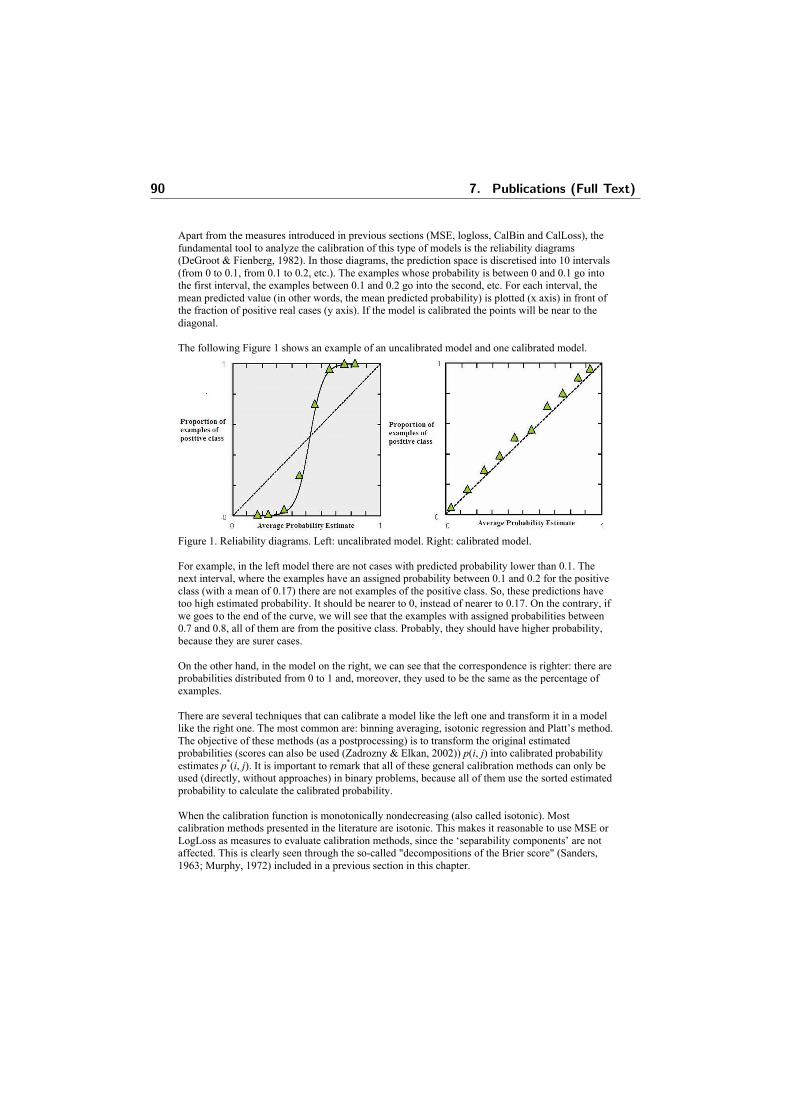
Apart from the measures introduced in previous sections (MSE, logloss, CalBin and CalLoss), the fundamental tool to analyze the calibration of this type of models is the reliability diagrams (DeGroot & Fienberg, 1982). In those diagrams, the prediction space is discretised into 10 intervals (from 0 to 0.1, from 0.1 to 0.2, etc.). The examples whose probability is between 0 and 0.1 go into the first interval, the examples between 0.1 and 0.2 go into the second, etc. For each interval, the mean predicted value (in other words, the mean predicted probability) is plotted (x axis) in front of the fraction of positive real cases (y axis). If the model is calibrated the points will be near to the diagonal. The following Figure 1 shows an example of an uncalibrated model and one calibrated model.

Figure 1. Reliability diagrams. Left: uncalibrated model. Right: calibrated model. For example, in the left model there are not cases with predicted probability lower than 0.1. The next interval, where the examples have an assigned probability between 0.1 and 0.2 for the positive class (with a mean of 0.17) there are not examples of the positive class. So, these predictions have too high estimated probability. It should be nearer to 0, instead of nearer to 0.17. On the contrary, if we goes to the end of the curve, we will see that the examples with assigned probabilities between 0.7 and 0.8, all of them are from the positive class. Probably, they should have higher probability, because they are surer cases. On the other hand, in the model on the right, we can see that the correspondence is righter: there are probabilities distributed from 0 to 1 and, moreover, they used to be the same as the percentage of examples. There are several techniques that can calibrate a model like the left one and transform it in a model like the right one. The most common are: binning averaging, isotonic regression and Platt’s method. The objective of these methods (as a postprocessing) is to transform the original estimated probabilities (scores can also be used (Zadrozny & Elkan, 2002)) p(i, j) into calibrated probability estimates p*(i, j). It is important to remark that all of these general calibration methods can only be used (directly, without approaches) in binary problems, because all of them use the sorted estimated probability to calculate the calibrated probability. When the calibration function is monotonically nondecreasing (also called isotonic). Most calibration methods presented in the literature are isotonic. This makes it reasonable to use MSE or LogLoss as measures to evaluate calibration methods, since the ‘separability components’ are not affected. This is clearly seen through the so-called "decompositions of the Brier score" (Sanders, 1963; Murphy, 1972) included in a previous section in this chapter.


Binning Averaging The first calibration method is called binning averaging (Zadrozny & Elkan, 2001) and consists in sorting the examples in decreasing order by their estimated probabilities and dividing the set into k bins (i.e. subsets of equal size). Then, for each bin l, kl ≤≤1 , the corrected probability estimate for a case i belonging to class j, p*(i, j), is the proportion of instances in l of class j. The number of bins must be small in order to reduce the variance of the estimates. In their paper, Zadrozny and Elhan fixed k=10 in the experimental evaluation of the method. Example: Consider the following training set sorted by its probability of membership to positive class grouped in 5 bins.

bin instance score 1

e1 e2 e3 e4

0.95 0.94 0.91 0.90

2

e5 e6 e7 e8

0.87 0.85 0.80 0.76

3

e9 e10 e11 e12

0.70 0.66 0.62 0.62

4

e13 e14 e15 e16

0.51 0.49 0.48 0.48

5

e17 e18 e19 e20

0.45 0.44 0.44 0.42

Then, if a new example is assigned a score of 0.68, then it belongs to bin 3 and its corrected

probability is 65.04

62.062.066.070.0=

+++ .

This is just how binning averaging works. Isotonic Regression (PAV) A slightly more sophisticated technique also for two-class problems is isotonic regression. (Ayer, Brunk, Ewing, Reid, & Silverman, 1955) presented a pair-adjacent violators algorithm (PAV) for calculating the isotonic regression. The idea is that calibrated probability estimates must be a monotone decreasing sequence, i.e., nppp ≥≥≥ ...21 . If it is not the case, the PAV algorithm each time that a pair of consecutive probabilities, p(i, j) and p(i + 1, j), does not satisfy the above property p(i, j) < p(i + 1, j) replaces both of them by their probability average, that is:


2),1(),(),1(),( ** jipjipjipjip ++

=+=

This process is repeated (using the new values) until an isotonic set is reached. Example. The next table shows in the first column the initial scores of one dataset composed by 10 examples. The following columns represent the results obtained in the steps given by the PAV method where the last one contains the calibrated probabilities. instance initial

score PAV step 1

PAV step 2

e1 0.76 0.765 0.765 e2 0.77 0.765 0.765 e3 0.70 0.705

0.705 0.705 0.705 e4 0.71

e5 0.66 0.685 0.685

0.686 0.686 0.686

e6 0.71 e7 0.69 0.69 e8 0.68 0.68 0.68 e9 0.48 0.485

0.485 0.485 0.485 e10 0.49

Platt’s Method (Platt, 1999) presents a parametric approach for fitting a sigmoid that maps estimated probabilities into calibrated ones. This method was developed to transform the outputs of a support vector machine (SVM) from the original values [ ]∞∞− , to probabilities, but can be extended to other types of models or probabilities variations. The idea consists on passing to the values a sigmoid function of the form:

BjipAejip

+×+= ),(

*

11),(

The parameters A and B are determined such that minimise the negative log-likelihood of the data. Platt’s method is most effective when the distortion in the predicted probabilities has a sigmoid form (as in the previous example). Isotonic regression is more flexible and can be applied to any monotonic distortion. Nevertheless, isotonic regression used to present overfitting problems in some cases. Also, all the above methods can use the training set or an additional validation set for calibrating the model. The quality of the calibration might depend on this possibility and the size of the dataset. This is a recurrent issue in calibration, and it has been shown that some methods are better than others for small calibration sets (i.e. Platt’s scaling is more effective than isotonic regression when the calibration set is small (Caruana & Niculescu-Mizil, 2004)). Other Related Calibration Methods Apart from the methods for obtaining calibrated probabilities, there exits other calibration techniques only applicable to specific learning methods. For instance, smoothing by m-estimate (Cestnik, 1990) and Laplace (Provost & Domingos, 2000) are another alternative ways of improving the probability estimates given by an unpruned decision tree. Probabilities are generated from decision trees as follows. Let T be a decision tree and l a leaf which contain n training


instances. If k of these instances are of one class (for instance, of positive class), then when T is

applied to classify new examples it assigns a probability of nkp = that each example i in l belongs

to the positive class. But using the frequencies derived from the count of instances of each class in a leaf might not give reliable probability estimates (for instance, if there are few instances in a leaf). So, for a two-class problem, the Laplace correction method replaces the probability estimate by

21'

+

+=nkp . For a more general multiclass problem with C classes, the Laplace correction is

calculated as Cn

kp+

+=

1' . As Zadrozny and Elkan (2001) say "the Laplace correction method adjusts

probability estimates to be closer to 1/2, which is not reasonable when the two classes are far from equiprobable, as is the case in many real-world applications. In general, one should consider the overall average probability of the positive class, i.e. the base rate, when smoothing probability estimates" (p. 610). Thus, smoothing by m-estimate consists in replacing the above mentioned

probability estimate by mnmbkp

+

⋅+=' where b is the base rate and m is the parameter for controlling

the shift towards b. Given a base rate b, Zadrozny and Elkan (2001) suggest using m such that 10=⋅mb .

Another related technique also applicable to decision trees is curtailment (Zadrozny & Elkan, 2001). The idea is to replace the score of a small leaf (i.e., a leaf with few training instances) by the estimate of its parent node, if it contains enough examples. If the parent node still have few examples, we proceed with its parent node and so on until to reach either a node sufficiently populated or the tree root. CALIBRATION METHODS FOR RD The regression case when the goal is to have that the expected output to be equal (or close) to the real average output (type RD), has been implicitly or explicitly considered in most regression techniques to date. This is so, because there are two numeric outputs (the predicted value and the real value), so, there is more variety of corrective functions to apply. First we are going to see which the problem is in this case. The idea can be depicted (see Figure 2) if we compare the behaviour of the test data, denoted by "real", and the model that we want to calibrate ("predicted"). In the figure, we show the behaviour of two models with a similar squared error.

Figure 2. Calibration of regression models. Left: an uncalibrated model. Right: a calibrated model.


As we said in the introduction, the characteristic of a calibrated model for type RD is that the errors are equally distributed for the different output values, in other words, the expected value from distinct functions between the predicted value and the real value must be the right according to the function. For example, the expected value of the difference between the estimated value (yest) and the real value (y) must be near to zero, so E(yest – y) = 0. If this value is less than 0, then the real values are a little higher that the estimated ones, in average, if this value is greater than 0, the real values are a little lower than the estimated ones. Most regression models used to have this difference quite well calibrated. On contrary, the expected value of the quotient between the estimated value and the real value should be near to one, so E(yest / y) = 1. If this quotient is greater than one, the error used to be positive for high values and negative for low values. Techniques such as linear regression use to give calibrated models, but others (nonlinear regression, local regression, neural networks, decision trees, etc.) can give uncalibrated models. Logically, in both cases, the errors can be corrected, for example, by decreasing the high values and increasing the low values. In general, the solution comes from obtaining some type of estimation of the decalibration function between the real values and the predicted values. One of the most common approximations consists on calculate a linear regression as in the previous plots in the Figure 2 and apply it to the model, with the aim of fitting the calibration. These calibrations used to

increase the mean squared error nyy est

2)( − , but can achieve to reduce the relative mean squared

error nymeany

yyest

est

×−−

))(()( 2

or the error tolerance.

When the decalibration function is nonlinear (but it has a pattern), the problem of calibration becomes more complex, and some kind of nonlinear or local regression is needed to calibrate the model. In these cases, it is not properly a calibration process but a meta-learner, with several stages (stacking, cascading, etc.). CALIBRATION METHODS FOR RP On type RP, the prediction is a probability density function, and it is this function what we need to improve. This is a much more complex problem since improving this type of calibration can be done by mangling the prediction estimates (i.e. the MSE can be increased as the result of calibrating). Consequently, a trade-off must be found. In (Carney & Cunningham, 2006), they approach the problem by formulating it as a multi-objective problem. The two objectives of sharpness (a classical quality criterion based on negative log-likelihood (NLL) and the Anderson-Darling (A 2) test over the probability integral transform, as a measure of pure calibration. FUTURE TRENDS Future trends on calibration include a clearer recognition of the effects calibration has and when and how the four types of calibration are related as well as how they relate to classical quality metrics. In particular, calibration and traditional measures are sometimes conflicting, and we need to use a couple of metrics (such as A2 and NLL in the case of type RP), or a hybrid one (such as MSEp in the case of type CP), to select the best model. In classification, most calibration methods we have analysed work for binary problems. As we have seen, most calibration methods are based on sorting the instances and/or making bins. But for more than two classes it is not so clear how to sort the instances or, more generally, how to make the bins. This is one of the reasons for which.the calibration problem has been less discussed. There are some works like (Zadrozny & Elkan, 2002) where the multiclass calibration problem has been studied,


but using approaches for reducing a multiclass problem to a set of binary problems and for finding an approximate solution for this problem. Another interesting research line consists in to study in depth the relationship between ROC analysis (or its counterpart for regression, REC analysis) and calibration. For instance, the use of repairing concavities techniques in ROC analysis (Flach & Wu, 2005) to solve conflicts between the original class ranking and the new estimated probabilities. Finally, type RP is a future trend on its own, since it is the most complex case which has been paid attention much more recently. CONCLUSIONS

In this chapter we have addressed the problem of predictive model calibration and we have presented the most known calibration techniques for classification and regression. We have shown that for classification, there are evaluation measures which are suitable for calibration (such as logloss, MSE, ...). And, also, there are another measures (for instance, accuracy) which are not good. Other measures are used in conjunction with calibration measures, especially the separability measures (AUC). Similarly, in regression, specific measures are needed to evaluate calibration, although must be usually accompanied by measures of sharpness. Calibration techniques are usually based on deriving a transformation which converts the values (on types CD and RD) or the probabilities (on types CP and RP) to better estimates. Very different transformation techniques have been devised in the literature, but they usually include some kind of binning or sorting in discrete cases (classification) or some kind of integral in the continuous cases (regression). REFERENCES Ayer, M., Brunk, H., Ewing, G., Reid, W., & Silverman, E. (1955). An empirical distribution function for sampling with incomplete information. Annals of Mathematical Statistics, 5, 641–647. Carney, M., & Cunningham, P. (2006). Making good probability estimates for regression. 17th European Conference on Machine Learning, LNCS: Vol. 4212 (pp. 582-589). Caruana, R., & Niculescu-Mizil, A.(2004). Data mining in metric space: an empirical analysis of supervised learning performance criteria. Tenth ACM SIGKDD International Conference on Knowledge Discovery and Data Mining (pp 69–78). Cestnik, B. (1990). Estimating probabilities: A crucial task in machine learning. Ninth European Conference on Artificial Intelligence (pp. 147–149). DeGroot, M. & Fienberg, S. (1982). The comparison and evaluation of forecasters. Statistician, 31(1), 12–22. Dowe, D. L., Farr, G. E., Hurst, A. J., & Lentin, K. L. (1996). Information-theoretic football tipping. 3rd Conference on Maths and Computers in Sport (pp 233-241). Fawcett, T. (2006), An introduction to ROC analysis. Pattern Recognition Letters, 27, 861–874.


Fawcett, T. & Niculescu-Mizil, A. (2007) PAV and the ROC convex hull. Machine Learning, 68(1), 97–106. Flach, P. A., & Matsubara, E. T. (2007). A simple lexicographic ranker and probability estimator. 18th European Conference on Machine Learning (pp. 575–582). Flach, P.A., & Wu, S. (2005). Repairing concavities in ROC curves. International Joint Conference on Artificial Intelligence (IJCAI'05) (pp. 702–707). Good, I. J. (1952). Rational decisions. Journal of the Royal Statistical Society. Series B 14, 107-114. Good, I. J. (1968). Corroboration, explanation, evolving probability, simplicity, and a sharpened razor. British Journal of the Philosophy of Science. 19, 123-143. Lachiche, N., & Flach, P.A. (2003) Improving Accuracy and Cost of Two-class and Multi-class Probabilistic Classifiers Using ROC Curves. International Conference on Machine Learning (pp. 416-423). Murphy, A. H. (1972). Scalar and vector partitions of the probability score: Part ii. n-state situation. Journal of Applied Meteorology, 11:1182–1192. Platt, J. C. (1999). Probabilistic outputs for support vector machines and comparisons to regularized likelihood methods. In P. J. Bartlett, B. Schölkopf, D. Schuurmans, and A. J. Smola, editors, Advances in Large Margin Classifiers (pp. 61–74). MIT Press, Boston. Provost, F., & Domingos, P. (2000). Well-trained PETs: Improving probability estimation trees (Technical Report CDER #00-04-IS). Stern School of Business, New York University. Sanders, F. (1963). On subjective probability forecasting. Journal of Applied Meteorology, 2, 191-201. Zadrozny, B., & Elkan, C. (2001). Obtaining calibrated probability estimates from decision trees and naive bayesian classifiers. Eighteenth International Conference on Machine Learning (pp. 609–616). Zadrozny, B., & Elkan, C. (2002). Transforming classifier scores into accurate multiclass probability estimates. Eighth ACM SIGKDD International Conference on Knowledge Discovery and Data Mining (pp. 694–699). KEY TERMS AND THEIR DEFINITIONS Calibration technique: is any postprocessing technique which aims at improving the probability estimation or to improve error distribution of a given model. Distribution calibration in classification (or simply "class calibration"): the degree of approximation of the true or empirical class distribution with the estimated class distribution. Probabilistic calibration for classification: the degree of approximation of the predicted probabilities to the actual probabilities.


Distribution calibration in regression: the relation between the expected value of the estimated value and the mean of the real value must be unbiased at the global and local levels. Probabilistic calibration for regression: when we have "density forecasting" models, a good calibration requires in general that these density functions are particular for each prediction, narrow when the prediction is confident and broader when it is less so. Calibration measure: any kind of quality function which is able to assess the degree of calibration of a predictive model. Confusion matrix: is a visual way of showing the recount of cases of the predicted classes and their actual values. Each column of the matrix represents the instances in a predicted class, while each row represents the instances in an actual class. Reliability diagrams. In these diagrams, the prediction space is discretised into 10 intervals (from 0 to 0.1, from 0.1 to 0.2, etc.). The examples whose probability is between 0 and 0.1 go into the first interval, the examples between 0.1 and 0.2 go into the second, etc. For each interval, the mean predicted value (in other words, the mean predicted probability) is plotted (x axis) in front of the fraction of positive real cases (y axis). If the model is calibrated the points will be near to the diagonal. BIOGRAPHY Antonio Bella finished his degree in Computer Science at the Technical University of Valencia in 2004 and started PhD studies in Machine Learning at the Department of Information System and Computation in the same university. At the same time, in 2005 he obtained a MSc in Corporative Networks and Systems Integration and in 2007 he started a degree in Statistical Science and Technology at the University of Valencia. Cèsar Ferri is an associate professor of computer science at the Department of Information Systems and Computation, Technical University of Valencia, Spain, where he has been working since 1999. He obtained his BSc at the Technical University of Valencia, and his MSc at the University of Pisa, Italy. His research interests include machine learning, cost-sensitive learning, relational data mining, and declarative programming. He has published several journal articles, books, book chapters and conference papers on these topics. José Hernández-Orallo, BSc, MSc (Computer Science, Technical University of Valencia, Spain), MSc (Computer Science, ENSEA, Paris), Ph.D. (Logic, University of Valencia). Since 1996, he has been with the Department of Information Systems and Computation, Technical University of Valencia, where he is currently an Associate Professor. His research interests centre on the areas of artificial intelligence, machine learning, data mining, data warehousing and software engineering, with several books, book chapters, journal and conference articles on these topics. María José Ramírez-Quintana received the BSc from the University of Valencia (Spain) and the Msc and PhD in Computer Science from the Technical University of Valencia (Spain). She is currently an associate professor at the Department of Information Systems and Computation, Technical University of Valencia. She has lectured several courses on software engineering, functional and logic programming, and multiparadigm programming. Her research interest include mutiparadigm programming, machine learning, data mining algorithms, model combination and evaluation, and learning from structured data, with more than 60 publications in these areas, including journal articles, books, book chapters and conference contributions.



7.4 Data Mining Strategies for CRM NegotiationPrescription Problems

4. A. Bella, C. Ferri, J. Hernandez-Orallo, and M.J. Ramırez-Quintana. DataMining Strategies for CRM Negotiation Prescription Problems. InTrends in Applied Intelligent Systems (IEA/AIE), volume 6096 of Lecture Notesin Computer Science, pages 520–530. Springer Berlin / Heidelberg, 2010.

Data Mining Strategies for CRM NegotiationPrescription Problems ?


DSIC-ELP, Universidad Politecnica de Valencia, Camı de Vera s/n, 46022 Valencia,Spain

Abstract. In some data mining problems, there are some input fea-tures that can be freely modified at prediction time. Examples happenin retailing, prescription or control (prices, warranties, medicine doses,delivery times, temperatures, etc.). If a traditional model is learned,many possible values for the special attribute will have to be tried toattain the maximum profit. In this paper, we exploit the relationshipbetween these modifiable (or negotiable) input features and the outputto (1) change the problem presentation, possibly turning a classificationproblem into a regression problem, and (2) maximise profits and derivenegotiation strategies. We illustrate our proposal with a paradigmaticCustomer Relationship Management (CRM) problem: maximising theprofit of a retailing operation where the price is the negotiable inputfeature. Different negotiation strategies have been experimentally testedto estimate optimal prices, showing that strategies based on negotiablefeatures get higher profits.

1 Introduction

In data mining, problem features (or attributes) have been usually classified asinput and output features. A problem is said to be supervised if it has outputfeatures, and it is said to be unsupervised if it does not have output features.Input features can be of many kinds: numerical, nominal, structured, etc. Infact, many data mining methods have been specialised to specific kinds of inputfeatures. In supervised learning, it is usually assumed that the goal of a modelis to predict an output value given an input. Consequently, a function is learnedfrom inputs to outputs, which is eventually applied to new cases.

However, in many application areas not all input feature values are given.This does not mean that they are unknown (i.e., null), but that they can be mod-ified or fine-tuned at prediction time. Consider a typical data mining problem: aloan granting model where loans are granted or not according to a model whichhas been learnt from previous customer behaviours. It is generally assumed thatgiven the input feature values (the customer’s personal information, the loanamount, the operation’s data, etc.) the model will provide an output (yes/no, aprobability, a profit, etc.). But in real scenarios, the decision of whether the loan

? This work has been partially supported by the EU (FEDER) and the SpanishMEC/MICINN, under grant TIN 2007-68093-C02 and the Spanish project ”Agree-ment Technologies” (Consolider Ingenio CSD2007-00022).

7.4. Data Mining Strategies for CRM Negotiation Prescription Problems 99

must be granted or not might change if one or more of the input feature valuescan be changed. Perhaps, a loan cannot be granted for 300,000 euros, but it canbe granted for 250,000 euros. If the customer asks the bank’s clerk “what is themaximum amount you can grant for this operation?”, we have a sort of inverseproblem. Since the model is not generally an analytical one (it is not generally alinear regression model but a neural network, SVM, decision tree or other kindof difficult-to-inverte models), the only possibility to give a precise answer to thecustomer is to try all the possible input combinations for the loan amount andfind out the maximum value which is granted. After this inefficient and ad-hocprocess, the clerk can give an answer such as: “According to our loan models,we can grant a maximum of 278,304 euros”. Apart from this inefficiency, thereis another more serious problem: the clerk knows that the model will give a neg-ative answer to any amount above this maximum, for instance, 278,305 euros,which makes this loan a quite risky one.

This typical example shows that some input features are crucial in the waythat they can be freely modified at prediction time. The existence of these specialattributes makes it quite inefficient to develop a classification/regression modelin the classical way, since whenever there is a new instance hundreds of possiblevalues have to be tried for the special attribute in order to see which combinationcan attain the maximum profit, or, as the previous example, the maximum risk.Additionally, these features are frequently associated to negotiation scenarios,where more than one attempt or offer have to be made, by suitably choosingdifferent values for this special input feature.

In this paper we analyse these special features that we call “negotiable fea-tures”, and how they affect data mining problems, its presentation and its usefor confidence probability estimation and decision making. As we will see, we canexploit the relation between these input features and the output to change theproblem presentation. In this case, a classification problem can be turned intoa regression problem over an input feature [1]. Also, we present a first generalsystematic approach on how to deal with these features in supervised models andhow to apply these models in real negotiation scenarios where there are severalattempts for the output value.

The paper is organised as follows. In Section 2 we focus on classificationproblems with one numerical negotiable feature, since this is the most frequentand general case, and it also includes prototypical cases, when the negotiablefeature is price or time. We present a general approach to the inversion prob-lem which transforms the classification problem into a regression one, where thenegotiable feature is placed as the output. In Section 3, we describe a specificreal scenario (an estate agent’s) where negotiation can take place. We also de-velop some negotiation strategies using the previous approaches in Section 4. InSection 5, we experimentally evaluate models and negotiation strategies with abaseline approach. Section 6 includes the conclusions and future work.

2 Inverting Problem Presentation

As we have mentioned in the introduction, there are many data mining problemswhere one or more input attributes, we call negotiable features, can be modified

2


at application time. Imagine a model which estimates the delivery time for anorder depending on the kind of product and the units which are ordered. Onepossible (traditional) use of this model is to predict the delivery time given anew order. However, another use of this model is to determine the number ofunits (provided it is possible to play with this value) that can be delivered in afixed period of time, e.g. one week. This is an example of an “inverse use” of adata mining model, where all inputs except one and the output are fixed, andthe objective is to determine the remaining input value.

The inversion problem can be defined as follows. Consider a supervised prob-lem, where input attribute domains are denoted by Xi, i ∈ {1, . . . ,m}, and theoutput attribute domain is denoted by Y . We denote the target (real) functionas f : X1 × X2 × . . . × Xm → Y . Values for input and output attributes willbe denoted by lowercase letters. Hence, labelled instances are then tuples of theform 〈x1, x2, . . . , xm, y〉 where xi ∈ Xi and y ∈ Y . The inversion problem con-sists in defining the function f I : X1× . . .×Xi−1× Y ×Xi+1× . . .×Xm → Xi,where Xi is the negotiable feature. In the above example, f is the function thatcalculates the delivery time of an order, the negotiable feature Xi is the numberof delivered units and f I calculates this number by considering fixed the deliverytime.

In the inverting problem the property that we call sensitive is satisfied.Fixing the values of all the other input attributes Xj 6= Xi for at least n examplesfrom the dataset D (n ≤ |D| being n determined by the user depending onthe problem, the presence of noise, . . . ), there are two different values for Xi

producing different output values.

We also assume a monotonic dependency between the input attribute Xi

and the output. This dependency is defined under the assumption that thereis a strict total order relation for the output, denoted by ≺, such that for ev-ery two different possible values ya, yb ∈ Y , we have that either ya ≺ yb oryb ≺ ya. This order usually represents some kind of profit, utility or cost. Fornumerical outputs, ≺ is usually the order relation between real numbers (either< or >, depending on whether it is a cost or profit). For nominal outputs, ≺usually sets an order between the classes. For binary problems, where POS andNEG represent the positive and negative class respectively, we can just set thatNEG ≺ POS. For more than two classes, the order relation can be derived fromthe cost of each class. Analogously, there is also a total order relation for theinput denoted as �. Based on this order, we can establish a monotonic depen-dency between the input and the output features. Thus, ∀a, b ∈ Xi, if a � bthen f(x1, . . . , xi−1, a, xi+1, . . . , xm) ≺ f(x1, . . . , xi−1, b, xi+1, . . . , xm) (mono-tonically increasing) or ∀a, b ∈ Xi, if a � b then f(x1, . . . , xi−1, a, xi+1, . . . , xm) �f(x1, . . . , xi−1, b, xi+1, . . . , xm) (monotonically decreasing).

The inversion problem is well-known [1] and seems simple at first sight, butmany questions arise. First, is f I also a function? In other words, for two differentvalues for Xi we may have the same value for Y which will ultimately translateinto two inconsistent examples for f I (two equal inputs giving different outputs).Second, the fact that we have an example saying that a given loan amount

3


was granted to a customer does not mean that this is the maximum amountthat could be granted to the customer. Third, deriving probabilities to answerquestions such as “which loan amount places this operation at a probabilityof 0.95 of being a profitable customer?” seem to be unsolvable with this newpresentation.

But if we take a closer look at these issues, we see that although relevant,there is still a possibility behind this problem presentation change. First, manyregression techniques work well for inconsistent examples, so this is not a bigpractical problem. Second, it is true that cases do not represent the maximumamount, but in many cases the examples represent deals and they are frequentlynot very far away from the maximum. Or, in the worst case, we can understandthe new task as “inferring” the typical value for Xi such that the loan is grantedto the customer. And third, we can also obtain probabilities in a regressionproblem. We extend this idea further below.

If we invert the problem, how can we address the original problem again?With the original model and for only two classes, it can be done by calculatingp(POS|〈x1, . . . , xi−1, a, xi+1, . . . , xm〉), for any possible value a ∈ Xi. From theinverted (regression) problem, we get: a = f I(x1, . . . , xi−1, POS, xi+1, . . . , xm).If we think of a as the predicted maximum or minimum for a which makes achange on the class, a reasonable assumption is to give 0.5 probability for this,that is p(POS|〈x1, . . . , xi−1, axi+1, . . . , xm〉) = 0.5.

The next step is to assume that the output for f I follows a distribution withcentre at a. For instance, we can assume a normal distribution with mean ata and use the standard error (mean absolute error, mae, on the training set)as standard deviation σ. In other words, we use N(a,mae2). Figure 1 shows anexample of a normal distribution with centre at a = 305, 677.9 and standarddeviation σ = 59, 209.06 and its associated cumulative distribution function.

Fig. 1. Left: Example of a normal distribution a = 305, 677.9 and σ = 59, 209.06.Right: Associated cumulative distribution function.

From here, we can derive the probability for any possible value a as thecumulative distribution function derived from the above normal, i.e., Φa,mae2 .

Consequently, for solving the original problem, (1) we solve the inversionproblem directly and (2) we use the predicted value of the negotiable feature as

4


mean of a normal distribution with the standard error as standard deviation.We call this model negotiable feature model.

3 Negotiation using Negotiable Feature Models: A RealScenario

We are going to illustrate the approach we have presented in the previous sectionin a real example. In particular, we have studied the problem of retailing, wherethe (negotiable) input feature is the price (denoted by π) and the problem is aclassification problem (buying or not).

We present an example using real data from an estate agent’s, which sells flatsand houses they have in their portfolio. We have several conventional attributesdescribing the property (squared metres, location, number of rooms, etc.), anda special attribute which is our negotiable feature, price. We will use the term“product” for properties to make it clear that the case is directly extensible tovirtually any retailing problem where price is negotiable.

We start with the simplest negotiation scenario, where there are only oneseller and one buyer who both negotiate for one product. One buyer is interestedin one specific product. S/he likes the product and s/he will buy the product ifits price is under a certain price that s/he is willing to pay for this product.Infact, if we reduce price to 0, the probability of having class POS approaches 1and if we increase price to a very large amount, the probability of having classNEG approaches 1. Moreover, the relation between price and the class orderNEG ≺ POS is monotonically decreasing.

Additionally, in our problem, the seller has a “minimum price” (denoted byπmin), which corresponds to the price that the owner has set when the productwas included in the portfolio plus a quantity that the seller sets as fixed andvariable costs. Any increment over this minimum price is profitable for the seller.Conversely, selling under this value is not acceptable for the seller. Therefore,the seller will not sell the product if its price is under this minimum price thats/he knows. Finally, the profit obtained by the product will be the differencebetween the selling price minus the minimum price: Profit(π) = π − πmin.

Obviously, the goal of the seller is to sell the product at the maximum possibleprice (denoted by πmax) which is the value such that the following equalities hold:

f(x1, . . . , xi−1, πmax, xi+1, . . . , xm) = POSf(x1, . . . , xi−1, πmax + ε, xi+1, . . . , xm) = NEG,∀ε > 0

In other words, the use for the model is: “Which is the maximum price that I cansell this product to this customer?”. Logically, the higher the price the lower theprobability, so the goal is more precisely to maximise the expected profit, whichis defined as follows:

E Profit(π) = p(POS|〈x1, . . . , xi−1, π, xi+1, . . . , xm〉) · Profit(π) (1)where p is the estimated probability given by the negotiable feature model.

To ease notation we will denote p(POS|〈x1, . . . , xi−1, π, xi+1, . . . , xm〉) asp(POS|π), consequently, we can express (1) as:

E Profit(π) = p(POS|π) · Profit(π) (2)with the additional constraint, as mentioned, that π ≥ πmin.

5


Fig. 2. Left: Example of estimated probabilities. Right: Associated expected profit.The minimum and maximum price are also shown.

So, if we have a model which estimates probabilities for the positive class, wecan use formula (2) to choose the price that has to be offered to the customer.If probabilities are well estimated, for all the range of possible prices, this mustbe the optimal strategy. In Figure 2 an example of the plots that are obtainedfor the estimated probabilities and expected profit is shown.

But this is the case where we have one bid (one offer). In many negotiationscenarios, we have the possibility of making several bids, as in bargaining. In thissituation, it is not so direct how to use the model in order to set a sequence ofbids to get the maximum overall expected profit. For instance, if we are allowedthree bids, the overall expected profit of a sequence of bids is defined as:

E Profit(〈π1, π2, π3〉) = p(POS|π1) ·Profit(π1)+(1− p(POS|π1)) · p(POS|π2) ·Profit(π2)+

(1− p(POS|π1)) · (1− p(POS|π2)) · p(POS|π3) · Profit(π3),

where π1 > π2 > π3 ≥ πmin.

4 Negotiation Strategies

In the scenario described in Section 3 the seller is the agent who uses the nego-tiable feature models to guide the negotiation, while the buyer can only makethe decision of buying or not the product.

When we have one possible offer, it is not sensible to set the price at themaximum price that our model predicts it can be sold, because in many cases,because of the prediction error, it will be overestimated and we will not sell theproduct. On the contrary, selling at the minimum price ensures that we sell asmany products as possible, but we get minimum profit as well. In Section 3 wesaw that an appropriate way of doing this is by using the expected profit.

Obviously, if the maximum price for the buyer is lower than the minimumprice for the seller, the product is not sold. We will exclude these cases, sinceany strategy is not going to work well for them and it is not going to make anydifference to include them or not in terms of comparison.

When we have more than one possible offer, we start with a first offer and ifthe price is less or equal than a price which is accepted by the buyer, s/he will

6


buy the product. Otherwise, the seller can still make another offer and followthe negotiation.

It is clear that there exists an optimum solution to this problem when theseller can make “infinite” offers to the buyer, but it is inefficient and unfeasible.This idea consists in beginning the negotiation with a very high offer and makeoffers of one euro less each time, until the (patient and not very intelligent) buyerpurchases the product or until the price of the product is the minimum price.In this case the product would be sold by its maximum price, because the buyerpurchases the product when the price offered was equal to the maximum priceconsidered by the buyer.

In what follows we propose several strategies. One is the “baseline” methodwhich is typically used in real estate agent’s. For cases with one single bid, weintroduce the strategy called “Maximum Expected Profit” (MEP), which is justthe application of the expected profit as presented in the previous section. Forcases with more bids (multi-bid) we present two strategies: “Best Local ExpectedProfit” (BLEP) strategy and “Maximum Global Optimisation” (MGO) strategy.Let us see all of them in detail below:

– Baseline method (1 bid or N bids). One of the simplest methods to price aproduct is to increase a percentage to its minimum price (or base cost). In-stead of setting a fix percentage arbitrarily, we obtain the percentage (calledα) such that it obtains the best result for the training set. For example ifwe obtain that the best α is 0.4, it is expected that the best profit will beobtained increasing in 40% the minimum price of the properties. If we haveonly 1 bid, we will increase the minimum price of the flat by α. But, if wehave N bids, we will have one half of the bids with a value of α less thanthe calculated α and the other half of the bids with a value of α greaterthan the calculated α. In particular, the value of α will increase or decreaseby α/(N + 1) in each bid. For example, for 3 bids and the previous samplethe three values of α for three bids would be 50%, 40% and 30%. Therefore,the first offer would be an increase of 50% over the minimum price of theproduct, the second an increase of 40% and the third an increase of 30%.

– Maximum Expected Profit (MEP) strategy (1 bid). This strategy is typ-ically used in marketing when the seller can only make one offer to thecustomer. Each price for an instance gives a probability of buying. Thisstrategy chooses the price that maximises the value of the expected profit.πMEP = argmaxπ(E Profit(π)).

– Best Local Expected Profit (BLEP) strategy (N bids). This strategy con-sists in applying the MEP strategy iteratively, when it is possible to makemore that one offer to the buyer. The first offer is the MEP, and if thecustomer does not accept the offer, his/her curve of estimated probabilitiesis normalised taking into account the following: the probabilities of buyingthat are less than or equal to the probability of buying at this price will beset to 0; and the probabilities greater than the probability of buying at thisprice will be normalised between 0 and 1. The next offer will be calculatedby applying the MEP strategy to the normalised probabilities. In the case

7


of the probability of buying which is associated to the price is the maximumprobability, it will not be set to 0, because the expected profit would alwaysbe 0. Instead of this, the next offer is directly the half of the price. Thepseudo-code is in Algorithm 1.

– Maximum Global Optimisation (MGO) strategy (N bids). The objective ofthis strategy is to obtain the N offers that maximise the expected profit bygeneralising the formula that we have presented in Section 3:πMGO = argmax〈π1,...,πN 〉(E Profit(〈π1, . . . , πN 〉) = argmax〈π1,...,πN 〉(p(POS|π1) ·Profit(π1) + (1 − p(POS|π1)) · p(POS|π2) · Profit(π2) + . . . + (1 − p(POS|π1)) · . . . · (1 −p(POS|πN−1)) · p(POS|πN ) · Profit(πN )).Getting the N bids from the previous formula is not direct but can be donein several ways. One option is just using a Montecarlo approach with asufficient number of tuples to get the values for the prices that maximise theexpected profit.

Algorithm 1: BLEP strategy

Require: N , epf (estimated probability function or curve)Ensure: πBLEB∀x, epf(x)← p(POS|x)π1 ← πMEBπ ← π1

for πi, i ∈ 2..N doif epf(π) 6= maxx∈0..∞(epf(x)) then∀x, epf(x)← 0if epf(x) 6 epf(π) thenepf ← normalise(epf, epf(π),maxx∈0..∞ epf(x)){normalise(f(x),mix,max): returns normalised function of f(x) from values min andmax to [0..1]}

end ifπi ← πMEBπ ← πi

elseπi ← π ÷ 2π ← πi

end ifend forπBLEB ← 〈π1, . . . , πN 〉

5 Experiments

5.1 Experimental Settings

Experiments have been performed by using real data collected from an estateagent’s. We have information of 2,800 properties (flats and houses) that weresold in the last months, for which we have the following attributes (“district”,“number of rooms”, “square metres” and the “owner’s price”). The “owner’sprice” is the price which the owner wants to obtain for the property.

In the experiments we have assumed that the “owner’s price” is some kind of“market price” and we have considered that it is the “maximum price”. Althoughit is not always true because in some cases the buyer could have paid more thanthis for the property.

We have randomly split the dataset into a training set and a test set. 10%of the data are for training and the rest to test. This tries to simulate a realistic

8


situation when there are not too many data for training. Therefore, the resultsrefer to 2,520 properties, and learning is made from 280 flats. We applied thesolutions proposed in Section 2 to the data. In particular we have used a J48decision tree1 (with Laplace correction and without pruning) implemented inthe data mining suite WEKA [3]. Since the predicted probability curve givenby a classifier (such as the J48 classifier) typically shows discontinuities andstrong steps when varying a negotiable feature, we have smoothed it with a low-pass filter with Bartlett overlapping window [2]. The parameter of the windowhas been set to the “minimum price” divided by 400. The “inversion problem”solution has been implemented with the LinearRegression and M5P regressiontechniques, also from WEKA.

These three learning techniques have been used to guide the three negotiationstrategies explained in Section 4 (for the MGO strategy we used a Montecarloapproach using 1,000 random triplets) and they are compared to the two baselinemethods also mentioned in Section 4. In the experiments the number of bids iseither one or set to three, i.e., N = 3. Summing up, we have nine negotiationmethods based on learning techniques and also two baseline methods (withoutlearning process) using the best possible α (80% for one bid and the triplet〈100%, 80%, 60%〉 for three bids).

5.2 Experimental Results

In Table 1 we can observe the results obtained for each method, in terms ofnumber of sold properties, total sold price (in euros) and total profit (in euros).

Table 1. Results obtained by the negotiation strategies, baseline methods and reference methods(minimum and maximum profit). Sold price and profit measured in euros.

Method Sold flats Sold price Profit

All flats sold at πmin 2,520 356,959,593 0All flats sold at πmax 2,520 712,580,216 355,620,623

1 bidBaseline (80%) 1,411 200,662,464 89,183,317

MEP (J48) 1,360 302,676,700 129,628,471MEP (LinearRegression) 1,777 354,973,300 159,580,109

MEP (M5P ) 1,783 358,504,700 161,736,313

3 bidsBaseline (100%, 80%, 60%) 1,588 264,698,467 124,483,288

BLEP (J48) 1,940 382,921,400 173,381,116BLEP (LinearRegression) 2,056 400,953,200 174,832,025

BLEP (M5P ) 2,063 404,009,700 176,874,221MGO (J48) 1,733 390,529,770 176,020,611

MGO (LinearRegression) 1,918 475,461,200 232,600,223MGO (M5P ) 1,906 476,171,900 234,259,509

As we see in Table 1 all the negotiation methods outperform the baselinemethods. For one bid, MEP is clearly better than the baseline method. Forthree bids, both BLEP and MGO are much better than the baseline method.Overall, MGO makes a global optimisation and hence get better results.

1 In this problem, we only have data of sold properties (positive class), therefore, wehave generated examples of the negative class with a price higher than the “owners’sprice”.

9


On the other hand, the regression techniques outperform the J48 decisiontree, so, for this problem the solution of inverting problem presentation out-performs the improved classifier solution. This is especially dramatic for MGO,which is the method that depends most on a good probability estimation. Thismeans that the inversion problem using a normal distribution to get the esti-mated probabilities turns out to be a very useful approach.

6 Conclusions

This paper introduces a number of new contributions in the area of data miningand machine learning which can be useful for many application areas: retailing,control, prescription, and others where negotiation or fine-tuning can take place.Nonetheless, the implications can affect other decision-making problems wheredata mining models are used.

The first major contribution is the analysis of the relation between negotiablefeatures and problem presentation, and more specifically the inversion problemwhich happens naturally when we have to modify or play with the negotiableattribute. We have seen that using the monotonic dependency we can change ofproblem presentation to do the inversion problem (such as changing a classifi-cation problem into a regression), where the original problem is now indirectlysolved by estimating probabilities using a normal distribution.

The second major contribution is its application to real negotiation problems.We have developed several negotiation strategies and we have seen how theybehave for one or more bids in a specific problem of property selling. We haveshown that our approach highly improves the results of the classical baselinemethod (not using data mining) which is typical in this area. In the end, weshow that the change of problem presentation (from classification into regressionproblem, using the negotiable feature, price, as output) gets the best results forthe case with one bid but also for the case with three bids.

Since this work introduces new concepts and new ways of looking at someexisting problems, many new questions and ideas appear. For instance, we wouldlike to analyse how to tackle the problem when there are more than one nego-tiable feature at a time, especially for the inversion problem approach (since wewould require several models, one for each negotiable feature).

Finally, more complex negotiation strategies and situations can be exploredin the future: the customer can counter-offer, several customers, etc.

References

1. L. Devroye, L. Gyorfi, and G. Lugosi. A Probabilistic Theory of Pattern Recognition(Stochastic Modelling and Applied Probability). Springer, 1997.

2. E.W. Weisstein. CRC concise encyclopedia of mathematics. CRC Press, 2003.3. I. H. Witten and E. Frank. Data Mining: Practical Machine Learning Tools and

Techniques with Java Implementations. Elsevier, 2005.

10


7.5. Quantification via Probability Estimators 109

7.5 Quantification via Probability Estimators

5. A. Bella, C. Ferri, J. Hernandez-Orallo, and M.J. Ramırez-Quintana. Quan-tification via Probability Estimators. IEEE International Conference onData Mining, 0:737–742, 2010.

Quantification via Probability Estimators ?


DSIC-ELP, Universitat Politecnica de Valencia, Camı de Vera s/n, 46022 Valencia,Spain

Abstract. Quantification is the name given to a novel machine learningtask which deals with correctly estimating the number of elements of oneclass in a set of examples. The output of a quantifier is a real value; sincetraining instances are the same as a classification problem, a natural ap-proach is to train a classifier and to derive a quantifier from it. Someprevious works have shown that just classifying the instances and count-ing the examples belonging to the class of interest (classify & count)typically yields bad quantifiers, especially when the class distributionmay vary between training and test. Hence, adjusted versions of classify& count have been developed by using modified thresholds. However,previous works have explicitly discarded (without a deep analysis) anypossible approach based on the probability estimations of the classifier.In this paper, we present a method based on averaging the probabilityestimations of a classifier with a very simple scaling that does performreasonably well, showing that probability estimators for quantificationcapture a richer view of the problem than methods based on a threshold.

1 Introduction

George Forman [4][5][6] has introduced and systematised a new supervised ma-chine learning task called ‘quantification’. Quantification is defined as follows:“given a labeled training set, induce a quantifier that takes an unlabeled test setas input and returns its best estimate of the class distribution.”[5]. For instance,consider a bank that has a credit risk assessment model (possibly a machinelearning classifier), and it is assigned a new portfolio of customers (e.g., 100,000new customers who originated from an agreement with a retailing company).A very important (and classical) question is to determine which customers thecredits will be granted to. However, before resolving all of these specific decisionmaking problems, the bank will typically require an assessment of how manycredits it will grant, i.e., the bank will need to quantify how many of the cus-tomers in the portfolio will have their credit approved. The accuracy of thisquantification is critical to assigning human and economical resources, long be-fore any specific decision is made. Also, the result of this estimation may affect

? This work has been partially supported by the EU (FEDER) and the SpanishMEC/MICINN, under grant TIN 2007-68093-C02, the Spanish project “AgreementTechnologies” (Consolider Ingenio CSD2007-00022) and the GVA project PROME-TEO/2008/051.


the thresholds that may be established for each particular operation since theassessment of the global risk can affect the way in which each local risk is man-aged (e.g. the policies will probably change if the plan was to work with 25,000positive results but we expect 50,000). The quantification problem can be foundin almost any area in data mining, such as failure detection, medical diagnosis,customer-relationship management, and retailing.

The task is closely related to classification since examples have the samepresentation (several input features and a nominal output feature), but it isdifferent in that we are not interested in the specific predictions for each instanceof an application dataset, but on the overall count of elements of a particularclass. Consequently, quantification is applied to a batch of examples, and not toa single example alone. Since the output of the quantification problem is a realvalue, it has a relation to regression, but the input of the regressor would be asingle example rather than a set of examples.

Quantification is a very frequent problem in real applications, so it is some-what surprising that nobody in the data mining community, until George For-man, recognised, baptised, and addressed this task on its own. In [4][5][6], Formandevelops several methods and defines new experimental settings to evaluate thetask, especially focussing on the cases where the training class distribution isdifferent to the test class distribution.

One of the first conclusions from these works is that the naıve solution calledclassify & count (CC) does not work well. Consequently, several other methodsare introduced, by properly adjusting the threshold and also scaling the result.Other methods are not based on CC but are still based on thresholds. However,there is another way to address the problem, which is to consider probabilityestimators instead of crisp classifiers. If a classifier estimates a class probabilityfor each example, the CC method becomes the probability estimation & average(P&A) method. Surprisingly, this approach is considered a “non-solution” inSection 3.4 in [4] and an “ill-conceived method” in Section 2.4 in [6]. The reasonfor this is clearly shown with an example: “For a well-calibrated classifier, theoutput value y = 70% indicates that, of the training cases that score similarly,approximately 70% were positive. Supposing a large test set contains the sameproportion of positives, as among those cases that score y = 70% ± ε, roughly70% would be positive. However, if we repeat the test with most of the negativecases removed at random, then the proportion of positives among the remainingtest cases scoring in this bin (y = 70% ± ε) would be much greater. Thus, theoutput of 70% would greatly underestimate the new P (+|y = 70%); and likewisefor every bin. Again, the end effect is that this method would underestimate athigh prevalence and overestimate at low prevalence, just like the CC method.As a result, the use of probability estimators has not been explored since it hasbeen considered a “non-solution”.

We agree with the rationale, but this does not necessarily imply that weshould not give adjusted versions of P&A a chance. If adjusted versions of CCwork, such as Forman’s AC and T50, we think we could explore similar (ordifferent) adjusting methods for P&A. In this paper, we present a simple scal-

2


ing method over P&A, called “Scaled Probability Average”, which shows verygood performance. A quantifier based on probability estimation is not basedon a threshold, so the appraisal of this threshold is not so critical. In fact, ourmethod depends on the quality of all the probabilities since it considers all theinformation that the classifier gives us about the dataset.

Summing up, the main contributions of this paper are that we introduceprobability estimation to the scene of quantification, and we derive a simplescaling method that shows good performance.

The paper is organised as follows. Section 2 introduces basic notation andterminology for the quantification problem and sets the quality measures forquantification. Section 3 derives the methods based on P&A, presents the plainversion Probability Average (which is actually a bad solution in general) andthen introduces the Scaled Probability Average method. These two methods areevaluated in Section 4 with a range of test class imbalances and then comparedto other quantification methods. Finally, Section 5 wraps up the paper with theconclusions and future work.

2 Notation and Previous Work

Given a dataset T , n denotes the number of examples, and c the number ofclasses. We will use i to index or refer to examples, so we will express i = 1 . . . nor i ∈ T indistinctly. f(i, j) represents the actual probability of example i to beof class j. We assume that f(i, j) always takes values in {0,1} and is not strictly a

probability but a single-label indicator function. With nj =n∑i=1

f(i, j), we denote

the number of examples of class j. π(j) denotes the prior probability of class j,i.e., π(j) = nj/n. When referring to a particular dataset T , we will use the

equivalent expression πT (j) =∑

i∈T f(i,j)

|T | . Given a classifier, p(i, j) represents

the estimated probability of example i to be of class j taking values in [0,1].π(j) denotes the estimated probability of class j which is defined as πT (j) =∑

i∈T p(i,j)|T | when referring to a dataset T . For the sake of readability, when c = 2,

we will use the symbols ⊕ for the positive class and for the negative class.Since the probabilities are complementary for two classes, we will focus on thepositive class. Cθ(i, j) is 1 iff j is the predicted class obtained from p(i, j) using athreshold θ. We can omit θ when it is embedded in the classifier or clear from the

context. When c = 2, we will use the following measures TP =n∑i=1

f(i,⊕)C(i,⊕),

TN =n∑i=1

f(i,)C(i,), FP =n∑i=1

f(i,)C(i,⊕), FN =n∑i=1

f(i,⊕)C(i,); we

will also use the ratios, tpr = TP/(TP + FN) and fpr = FP/(FP + TN).We will use pos for the actual proportion of positives, i.e., π(⊕); and we willuse neg for the actual proportion of negatives, i.e., π(). Finally, the functionclip(X, a, b) truncates a real value X inside an interval [a, b]. We represent theelements of T of class ⊕ and with T⊕ and T, respectively.

3


2.1 Quantification

Forman [4][5][6] was the first to identify and name the quantification prob-lem: “quantification is accurately estimating the number of positives in the testdataset as opposed to classifying individual cases accurately.” Therefore, themain objective in a quantification task is to estimate the class distribution inthe target population from the distribution observed in the training dataset. Thisproblem is especially important in many application areas, such as medicine, riskassessment, diagnosis, etc., where the training dataset does not represent a ran-dom sample of the target population (because population changes over time orthe classes are highly imbalanced, with the positive class as a minority).

As Forman pointed out, quantification is a machine learning task that is quitedifferent from classification. In quantification, we are interested in the test setas a whole in order to determine its class distributions and not in the individualpredictions for each example. In fact, although accurate classifications generallygive accurate class counting, an inaccurate classifier can also be a good quantifierif false positives and false negatives cancel each other. In [6], Forman introducedseveral quantification methods that we arrange into the following three groups:

– Methods based on counting the positive predicted examples. The classify &count (CC) and the adjusted count (AC) methods belong to this group.

– Methods based on selecting a classifier threshold, but in this case, the thresh-old is determined from the relationship between tpr and fpr in order toprovide better quantifier estimates. For instance, some methods choose oneparticular threshold, such as: the X method, which selects the threshold thatsatisfies fpr = 1 − tpr; the Max method, which selects the threshold thatmaximises the difference tpr − fpr; or those methods like T50 that select aparticular rate between tpr and fpr. The Median Sweep (MS) method1 isanother method that tests all the thresholds in the test set, estimates thenumber of positives in each one, and returns a mean or median of theseestimations.

– Methods based on a mixture of distributions. The Mixture Model (MM)[4] isincluded in this group. It consists of determining the distributions from theclassifier scores on the training positive (D⊕) and negative examples (D)and then modelling the observed distribution D on the test set as a mixtureof D⊕ and D.

The best results are obtained with AC in general; however, when the train-ing sets are small and the number of positives is small, other methods such asT50 or MS can get better results (at the cost of performing worse in othermore balanced situations). Of the above-mentioned methods proposed by For-man, the simplest one is the CC method. It consists of learning a classifier fromthe training dataset and counting the examples of the test set that the clas-sifier predicts positive (

∑i∈Test C(i,⊕)). This method gives poor results since

it underestimates/overestimates the proportion of positives, unless the classifier

1 It is proposed when the tpr and fpr are estimated from cross-validation.

4


is perfect (tpr = 1 and fpr = 0). The AC method is an improvement of theCC method, which estimates the true proportion of positives pos by applying

the equation pos = pos′−fprtpr−fpr , where pos

′is the proportion of predicted positives


|Test| . Forman proposed estimating tpr and fpr by cross-validation on

the training set. Since this scaling can give negative results or results above 1,the last step is to clip pos to the range [0..1]. Finally, T50 is another methodthat selects the threshold where tpr = 50% and the rest works the same as AC.This method supposedly behaves better when the denominator in the formula ofpos is unstable with AC. We have implemented these three methods in order tofairly compare the performance of our proposals with them. The reason for thischoice is that these methods are the ones that are most related to ours and theirperformance is good, or very good, with respect to other quantification methodssuch as X, Max, or MS. In other words, they are representative of the state-of-the-art in quantification. Motivated by the fact that in quantification only oneresult per dataset is produced, Forman proposed an experimental methodologyto evaluate quantification that is different from the one that is normally used forclassification. It consists in varying the class distribution between the trainingset and the test set. For the training set, Forman randomly selected the numberof positive and negative examples from a range. For the test set, he varied thepercentage of positive examples to also cover scenarios with imbalanced classes.

As we have mentioned in the introduction, a natural approach to solve thequantification problem that Forman disregarded is to use a probability estimatorinstead of a classifier. But, we will show that there is a different way to estimatethe positive proportion by using probability estimations sharing the spirit of theCC method.

Moreover, our proposal is supposed to be more robust to variations in theprobability estimation of few examples than other methods based on thresholdsbecause we take into account all the information from the dataset. For exam-ple, consider a test set with probabilities and actual classes as follows: (0.90,+),(0.55,+), (0.53,−), (0.51,−) and (0.21,−). If we set the threshold at 0.6, the pro-portion of positives is 20%; however, if the threshold is 0.5, then the proportionof positives is 80%. Note that this is a good classifier, with perfect ordering,i.e., AUC=1. Therefore, methods that use thresholds are less robust in the sensethat a change in the estimation of few examples could cause a small shift in thethreshold but a large variation in the positive count estimation. However, re-garding the probabilities of all the examples, the proportion of positives is 54%.In order to have a large change here, many probability estimations would haveto change significantly.

2.2 Quantification Evaluation

We use two global evaluation measures from the classical error measures forcontinuous variables, the Mean Absolute Error (MAE) and the Mean SquaredError (MSE) for quantification. Forman only used the absolute error in hisexperiments, but we consider that the MSE measure is a better way to quantify

5


differences between estimations for real values. Let us formalise these measuresin order to better establish the quantification problem and goal.

Consider that we have a method that estimates the proportion of elementsfor each class (πT (j)). By calculating the absolute difference of these two values,we have the global MAE for each class, GMAEj(T ) = |πT (j)− πT (j)|, and forall the classes we have GMAE(T ) = 1

c ·∑j=1..cGMAEj(T ). Similarly, we cal-

culate GMSEj(T ) (πT (j)− πT (j))2

and GMSE(T ) = 1c ·

∑j=1..cGMSEj(T ).

For binary problems, we have that GMAE⊕ = GMAE = GMAE and alsothat GMSE⊕ = GMSE = GMSE. Therefore, for binary problems, we willonly evaluate the error for the proportion of positives.

3 Quantifying by Scaled Averaged Probabilities

The idea of using an average of the probability estimations is supported bythe issue that probabilities represent much richer information than just the de-cisions, which are simply derived information from the probability estimationusing a threshold. After this rationale, the use of probabilities shapes a familyof methods that we call probability estimation & average. The simplest methodin this family is called Probability Average (PA). First, a probabilistic classifieris learned from the training data, such as a Probability Estimation Tree or aNaıve Bayes model. Then, the learned model is applied to the instances in thetest set, obtaining a probability estimation for each one. Finally, the average ofthe estimated probabilities for each class is calculated. Although this definitionis multiclass, for the rest of the paper we will concentrate on binary datasets.In this case, we only need to care about one class (the positive class), and the

method is defined as follows: πPATest(⊕) =∑

i∈Testp(i,⊕)

|Test| .

Logically, if the proportion of positive examples in the training set is differentfrom the proportion of positive examples in the test set, the result will not besatisfactory in general. The solution comes precisely from the analysis of theextreme case when all the elements in the test set are of one class. In this case,we will get the average probability for the positive cases alone, which can onlybe 1 for a perfect classifier (which is not frequently the case). As in the ACmethod, the idea is to use a proper scaling.

Nevertheless, from the training set, it is possible to calculate the actual pro-portion of positive examples (πTrain(⊕)), the positive probability average (πTrain(⊕)),the positive probability average for the positives (πTrain⊕(⊕)), and the positiveprobability average for the negatives (πTrain(⊕)).

From the definitions, it is easy to check the following: πTrain⊕(⊕)·πTrain(⊕)+πTrain(⊕) · (1− πTrain(⊕)) = πTrain(⊕).

From this equation, we derive πTrain(⊕) =πTrain(⊕)−πTrain (⊕)

πTrain⊕ (⊕)−πTrain (⊕) , which

yields a probabilistic version of Forman’s adjustment (see Fig.1). When all arepositives, πTrain⊕(⊕) sets the maximum, and we scale this to 1. When all arenegatives, πTrain(⊕) sets the minimum, and we scale this to 0.

6


Thus, we propose a new quantification method, which we call Scaled Prob-ability Average (SPA), applying this last formula (scaling) in the same way asForman to the value obtained with the PA method (πPATest(⊕)), i.e., πSPATest (⊕) =πPATest(⊕)−πTrain (⊕)

πTrain⊕ (⊕)−πTrain (⊕) .

πSCCTest (⊕) =


|Test| −πTrain (⊕)

πTrain⊕ (⊕)−πTrain (⊕)

we will get the average probability for the positive cases alone, which can only

be 1 for a perfect classifier (which is not frequently the case). As in the Adjusted

Count (AC) method, the idea is to use a proper scaling.

Nevertheless, from the training set, it is possible to calculate the actual pro-

portion of positive examples (!Train(!)), the positive probability average (!Train(!)),

the positive probability average for the positives (!Train!(!)), and the positive

probability average for the negatives (!Train"(!)).

From the definitions, it is easy to check the following: !Train!(!)·!Train(!)+

!Train"(!) · (1" !Train(!)) = !Train(!).

From this equation, we derive !Train(!) =!T rain(!)"!T rain" (!)

!T rain! (!)"!T rain" (!) , which

yields a probabilistic version of Forman’s adjustment (see Fig.1). When all are

positives, !Train!(!) sets the maximum, and we scale this to 1. When all are

negatives, !Train"(!) sets the minimum, and we scale this to 0.

Thus, we propose a new quantification method, which we call Scaled Prob-

ability Average (SPA), applying this last formula (scaling) in the same way as

Forman to the value obtained with the PA method (!PATest(!)), i.e., !SPA

Test (!) =

!P AT est(!)"!T rain" (!)

!T rain! (!)"!T rain" (!) .

0

0

1

10.3 0.540.4 0.8 0.9

0.23 0.4 0.83

!Train(!)

!Train!(!)!Train(!)!Train"(!)


In the same way as in the SPA method the proportion of positive examples

estimated by the PA method is scaled, also this scaling can be applied to the

10


In the same way as in the SPA method, the proportion of positive examplesestimated by the PA method is scaled. This scaling can also be applied to theproportion of positive examples estimated by the CC method. Therefore, wepropose the Scaled Classify & Count (SCC) method.

4 Experiments

In this section, we present an experimental evaluation of several quantificationmethods: those based on classification (i.e., on a threshold), namely CC, AC, T50(explained in Section 2); our two methods based on probability average, namelyPA and SPA; and a hybrid method (SCC), which is explained in Section 3. Wehave not used an internal cross-validation process with the training set to betterestimate the thresholds, tpr and fpr, as Forman does. Instead, we have used anadditional validation set to estimate the thresholds, tpr and fpr. In other words,the methods are the same, but instead of using a 50 fold cross-validation processwith the training set, we have used two different sets (training and validation)and repeated the process 100 times.

The experimental setting is based on the common case where we train aclassifier or probability estimator on a training dataset and we want to quantifythe number of examples of one class for a different test dataset. We are especiallyinterested in cases where class distributions vary between training and test. Inorder to get this variation (and being able to consider cases where the majorityclass examples are increased or reduced), for each problem, we divided the wholedataset into 37.5% for training, 37.5% for validation, and 25% for test. Withthis original test set, we constructed six different variations test sets: the whole

7


0 20 40 60 80 100

0.00

0.02

0.04

0.06

0.08

3−CreditR., GMSE, Pi_{Train}(+)=45%

^Pi_{Test}(+)

GM

SE

^ ^ ^ ^ ^

CCACT50SCCPASPA

0 20 40 60 80 100

0.00

0.05

0.10

0.15

Mean all datasets, GMSE, Pi_{Train}(+)=39%

^Pi_{Test}(+)

GM

SE

^ ^ ^ ^ ^

CCACT50SCCPASPA

0 20 40 60 80 100

0.0

0.1

0.2

0.3

0.4

0.5


^Pi_{Test}(+)

GM

SE

^ ^ ^ ^ ^

CCACT50SCCPASPA

0 20 40 60 80 100

020

4060

8010

0

3−CreditR., GMSE, Pi_{Train}(+)=45%

^Pi_{Test}(+)*100

Pi_

{Tes

t}(+

)*10

0

^ ^ ^ ^ ^

CCACT50SCCPASPADiag.

0 20 40 60 80 100

020

4060

8010

0


^Pi_{Test}(+)*100

Pi_

{Tes

t}(+

)*10

0

^ ^ ^ ^ ^


0 20 40 60 80 100

020

4060

8010

0


^Pi_{Test}(+)*100

Pi_

{Tes

t}(+

)*10

0

^ ^ ^ ^ ^


Fig. 2. Upper-Left: GMSE results with variable test positive ratios for the dataset CreditR. Upper-Centre: GMSE results with variable test positive ratios for the average of all the datasets. Upper-Right: GMSE results with variable test positive ratios for the average of all the datasets, with theproportion of positive examples in the training and validation sets reduced by 90%. Lower-(Left,Centre and Right): The value of each quantification method for each test setting. The diagonalshows the perfect value.

8


Table 1. GMSE measure for each dataset and the average result of all the datasets for each quan-tification method, and MSE, AUC, CalBin and Accuracy measures for each dataset.

# Datasets Size πTr(⊕) CC AC T50 SCC PA SPA MSE AUC CalBin Acc.

1 W.B. Cancer 699 0.34 0.0022 0.0008 0.0667 0.0008 0.0032 0.0006 0.04 0.82 0.04 0.952 Chess 3196 0.48 0.0033 0.0002 0.0155 0.0024 0.0116 0.0001 0.06 0.82 0.09 0.933 Credit R. 690 0.45 0.0219 0.0046 0.0115 0.0070 0.0286 0.0037 0.15 0.76 0.16 0.824 German C. 1000 0.31 0.0921 0.0265 0.0277 0.0598 0.0878 0.0176 0.24 0.65 0.26 0.655 Pima D. 768 0.35 0.0572 0.0160 0.0247 0.0332 0.0642 0.0099 0.21 0.69 0.23 0.706 House V. 435 0.38 0.0044 0.0018 0.0522 0.0018 0.0048 0.0014 0.07 0.81 0.07 0.927 Monks1 556 0.49 0.0449 0.0072 0.0186 0.1025 0.0487 0.0057 0.16 0.72 0.23 0.798 Mushroom 8124 0.48 0.0268 0.0004 0.0380 0.0022 0.0211 0.0003 0.12 0.80 0.13 0.849 Spam 4601 0.39 0.0118 0.0003 0.0284 0.0006 0.0156 0.0003 0.10 0.80 0.10 0.8810 Tic-tac 958 0.34 0.0626 0.0107 0.0127 0.0525 0.0671 0.0062 0.19 0.71 0.23 0.7211 Breast C. 286 0.29 0.1280 0.1118 0.1171 0.1638 0.1057 0.0829 0.28 0.60 0.31 0.6212 Haberman B. 306 0.27 0.2045 0.1478 0.1265 0.2555 0.1316 0.1049 0.28 0.59 0.31 0.6013 Heart D. 303 0.45 0.0236 0.0108 0.0235 0.0116 0.0291 0.0083 0.15 0.75 0.17 0.8014 Heart S. 270 0.43 0.0251 0.0141 0.0352 0.0152 0.0320 0.0111

¯0.15 0.75 0.18 0.80

15 Ionosphere 351 0.35 0.0429 0.0075 0.0446 0.0068 0.0487 0.0053 0.17 0.75 0.19 0.8116 Monks2 601 0.34 0.2386 0.1826 0.2146 0.3087 0.1168 0.1732 0.27 0.55 0.31 0.5217 Monks3 554 0.48 0.0010 0.0004 0.0151 0.0069 0.0151 0.0006 0.05 0.82 0.13 0.9718 Hepatitis 155 0.19 0.1536 0.1241 0.1329 0.1454 0.1226 0.0885 0.27 0.66 0.30 0.6619 Sonar 208 0.46 0.0525 0.0460 0.0622 0.0521 0.0572 0.0400 0.26 0.67 0.27 0.6920 Spect 80 0.49 0.1009 0.0921 0.1308 0.1530 0.0722 0.0879 0.24 0.68 0.27 0.70

AVG. 0.39 0.0649 0.0403 0.0599 0.0691 0.0542 0.0324 0.17 0.72 0.2 0.77

test set with the original proportion of classes, and five test sets changing theproportion of classes (100% of examples of positive class and 0% of negative class,75% and 25%, 50% and 50%, 25% and 75%, and 0% and 100%). The proportionswere obtained by random undersampling using a uniform distribution.

In order to have a broad range of classifiers and probability estimators, weused four different methods from WEKA [7]: NaıveBayes, J48 (a C4.5 implemen-tation), IBk (k = 10) (a k-NN implementation), and Logistic (a logistic regres-sion implementation). We used the WEKA default parameters in the methods(except the parameter k in the IBk method that is set to 10). A total of 100repetitions were performed for each dataset (25 for each classifier). We selected20 binary datasets (Table 1) from the UCI repository [1]. We adopted the samecriterion as Forman, and the positive class is the minority class.

In Table 1, we show the results with respect to the GMSE measure2 for eachmethod. These values are the average of the 100 repetitions for each dataset.We also include MSE, AUC, CalBin and Accuracy measures (see, e.g. [3] for adefinition of these measures). For each dataset, as suggested in [2], we calculateda Friedman test and showed that the six methods do not have identical effects, sowe calculated the Nemenyi post-hoc test to compare all the methods with eachother (with a probability of 99.5%). The values in bold show that this methodoutperforms the others and that the difference is statistically significant. Also, ifseveral values are underlined, this indicates that these methods outperform the

2 GMAE results portray a similar picture.

9


rest with a statistically significant difference, but the difference between the twois not significant.

The results are categorical as far as the use of probability estimators. Not only dothey work, but they outperform all the other methods. Of course, as we expected,a proper scaling is the key to success. In the same way that AC dramaticallyimproves CC, SPA also improves PA. However, by looking at the table in moredetail we can get more insight. For instance, while CC and PA are relativelyclose, SPA is able to improve PA more than AC is able to improve CC (inrelative terms). The reason may be found in the way that SPA is not basedon thresholds (or measures such as tpr or fpr which depend on them), but onaverages. Thus, the results show that SPA is more robust. Regarding the othermethods, SCC is a hybrid method that uses classification to estimate the baseproportion and uses the probability average to scale it. The result shows no clearimprovement over CC or PA. This supports the thesis that, for SPA, it is theconjunction of PA with the scaling what makes the results good. The behaviourof T50 is expected, since it highly depends on the threshold and this is a methodoriented to cases where the original training set is highly imbalanced.

In order to analyse the effect of imbalance (in the training set), we repeatedthe experiments but reduced the number of examples of the positive class by90% in the training and validation sets. In this situation, the SPA method stillobtains good results, but, in most cases, the differences between the SPAmethodand the AC and T50 methods are not statistically significant. We want to remarkthat AC and T50 methods are designed for situations where the proportion ofclasses are imbalanced. Even though, this second experimental setting is morefavourable for the AC and T50 methods, SPA method still obtains good results.These results are summarised in Fig.2 (right).

Finally, in order to analyse the effect with respect to test imbalance, foreach dataset, we analysed the results for the six different test set imbalances.The conclusion was that the behaviour is similar in all the datasets. The bestresults (as expected) are obtained with class proportions that are close to theoriginal class proportion or close to 0.5, and much worse as we get closer to 0or 1 proportions. In Fig.2 (left), we show a typical case of a dataset where theerrors are much lower when the test proportion is close to the original trainingproportion. In Fig.2 (centre), we show the average results for the 20 datasetswithout reducing the proportion of examples of the positive class in the trainingset. In Fig.2 (right), we show the results of reducing the proportion of examplesof the positive class by 90% in the training and validation sets. Fig.2 (centre)shows that when the proportion of examples of the positive class in the test setis more or less between 20% and 60%, the AC method is the one that obtainsthe best results. In the rest of proportions, the SPA is the best method becauseits behaviour is always quite similar. With this in mind, it is logical to think interms of a new “mixed” method, which uses the method that obtain the bestresults in each interval. We have not implemented this method, but we proposeits implementation and experimental evaluation as an interesting topic for futurework.

10


5 Conclusions and Future Work

Quantification is an old and frequent problem that has only very recently re-ceived proper attention as a separate machine learning task. In our opinion, oneof the most natural ways to address the problem is to average the probabilityestimations for each class because we use all the information provided by theprobability estimator and because we do not rely so much on a good thresholdchoice. However, in the same way that CC does not work, this easy approachdoes not work. Since CC can be adjusted, we have seen that a simple probabilityaverage method can also be adjusted. We have derived a generalisation of For-man’s scaling for probabilities, and we have derived a new method from it. Theresults are highly positive and show that the use of probability estimators forquantification is good to pursue, which can lead to new methods in the future.

As further future work, there are obviously several areas (cost quantification[6]) and experimental settings (very imbalanced training datasets) that are bor-rowed from Forman’s seminal works for which a more exhaustive evaluation ofour methods and the derivation of specialised ones should be addressed. One ofthese extensions is quantification for more than two classes. Our PA method isoriginally multiclass, but the scaling used in SPA is not. We think that propermethods (different to indirect 1vs1 or 1vsall) could be derived using probabilityaveraging.

Finally, quantification for regression is also a machine learning task thatshould be investigated (as we stated in the introduction with the credit assess-ment problem, where an estimation of the total amount for a customer portfolioand not the number of granted credits would be the goal). In fact, quantificationfor regression might be closer to quantification through probability averagingthan through classification.

References

1. C.L. Blake and C.J. Merz. UCI repository of machine learning databases, 1998.2. J. Demsar. Statistical comparisons of classifiers over multiple data sets. Journal of

Machine Learning Research, 7:1–30, January 2006.3. C. Ferri, J. Hernandez-Orallo, and R. Modroiu. An experimental comparison of

performance measures for classification. Pattern Recogn. Lett., 30(1):27–38, 2009.4. G. Forman. Counting positives accurately despite inaccurate classification. In

ECML, pages 564–575, 2005.5. G. Forman. Quantifying trends accurately despite classifier error and class imbal-

ance. In KDD, pages 157–166, 2006.6. G. Forman. Quantifying counts and costs via classification. Data Min. Knowl.

Discov., 17(2):164–206, 2008.7. I. H. Witten and E. Frank. Data Mining: Practical Machine Learning Tools and

Techniques with Java Implementations. Elsevier, 2005.

11


7.6. Local and Global Calibration. Quantification using Calibrated Probabilities121

7.6 Local and Global Calibration. Quantificationusing Calibrated Probabilities

6. A. Bella, C. Ferri, J. Hernandez-Orallo, and M.J. Ramırez-Quintana. Local andGlobal Calibration. Quantification using Calibrated Probabilities. Technicalreport, DSIC-ELP. Universitat Politecnica de Valencia, 2010.

Local and Global Calibration. Quantificationusing Calibrated Probabilities


DSIC-ELP, Universitat Politecnica de Valencia, Camı de Vera s/n, 46022 Valencia,Spain

Abstract. In this document we present an study of calibration meth-ods for quantification that complements the paper “Quantification viaProbability Estimators” [3].

1 Quantification and Calibration

Given the results of the Section IV in [3], a question that arises is the impact ofhaving good probability estimators for quantification, since the method proposedin Section III in [3] is based on a probability average. [7][8][9] discusses that somebad classifiers can be good quantifiers, but also (and frequently) that some goodclassifiers can be very bad quantifiers. The key issue to understand this whenwe use classify & count and related methods is how the threshold is chosen.The key issue to understand this when we use average probability methods iscalibration [4][5][11][14][2]. A random, but well-calibrated classifier can give verygood results with the SPA method, when training and test class distributionsmatch. On the contrary, a very good classifier, with high separability (e.g. a highAUC) can have very bad calibration and give very bad quantification results withthe SPA method. But there are some other, more surprising cases. Considerthe worst classifier possible, which in the binary case outputs p(i,⊕) = 1 forevery example i of class and outputs p(i,⊕) = 0 for every example i of class⊕. If the dataset is balanced, quantification will be perfect. But calibrationin this case is extremely poor. As a result, calibration plays a very importantrole for quantification using probabilities, but the phenomenon is more complexthan it seems at first sight, even in the easy cases where training and test classdistributions are equal.

1.1 Local and Global Calibration

The first intuition from the previous discussion is that we do not need to havegood calibration for every single prediction to have an overall good quantificationresult. This suggests the distinction of what we call local (traditional) calibrationand global calibration. Let us see local calibration first.

A probability estimator is said to be perfectly calibrated [5] if as the numberof predictions goes to infinity, the predicted probability p(i, j) goes to the em-pirical probability. In other words, the expectation of example i to be of class j


is indeed p(i, j). Note that this does not mean that a classifier derived from theestimator is always correct. In fact, an estimator always outputting p(i,⊕) = 0.5for every i for a balanced binary problem (with classes ⊕ and ) is completelyuseless but perfectly calibrated.

Since the previous definition is based on an expectation or an empirical prob-ability, this logically depends on a distribution. This means that a classifier canbe perfectly calibrated with respect to a distribution but not with respect toa different distribution. For instance, the previous perfectly calibrated classi-fier always outputting p(i,⊕) = 0.5 becomes poorly calibrated if the problemdistribution changes to a situation where classes are now highly imbalanced.

Instead of distributions, we will talk about datasets, and we will define perfectcalibration in a more specific way using the notion of bin:

Definition 1. Given a dataset D, a set B ⊂ D is an ε-bin if ∀j ∈ C and∀i, k ∈ B, |p(i, j)− p(k, j)| ≤ ε, where C are the classes of the dataset.

A 0-bin is any set such that all the elements in the bin have the same estimatedprobability. An ε-bin B is maximal if there is no other ε-bin B′ such that B ⊂ B′.The value ε is called the calibration width and it is naturally assumed to be lessthan or equal to 1. From here we define perfect calibration as follows:

Definition 2. A probability estimator is ε-calibrated for a dataset D with atolerance τ iff for every maximal ε-bin B we have that:

∀j∣∣∣Pi∈B p(i,j)|B| −

Pi∈B f(i,j)|B|

∣∣∣ ≤ τ

We need to explain the meaning of both τ and ε. The meaning of τ is a degreeof accordance or tolerance between the expected frequency in a bin and theactual probability. This is, then, a calibration measure. When τ = 0 we talkabout perfect calibration. The meaning of τ is hence similar to existing measuresof degrees of calibration, such as ‘calbin’ and the calibration component in theBrier’s score [12][10], which are also based on the notion of binning (as well assome calibration methods (see e.g. [14][6])).

The meaning of ε is different and regulates the granularity/strictness of thebins. In fact, we can talk about local (traditional) calibration when ε = 0 andwe can talk about global calibration when ε = 1. Or, more precisely, we cantalk about different degrees of local/global calibration, with 0-calibration beingthe extreme point for local calibration and 1-calibration being the other extremepoint for global calibration.

Let us see some examples. Consider for instance a binary probability estima-tor with values:

Example 1.p(1,⊕) = 1 with f(1,⊕) = 1 p(5,⊕) = 0.75 with f(5,⊕) = 1p(2,⊕) = 0.75 with f(2,⊕) = 1 p(6,⊕) = 1

3 with f(6,⊕) = 1p(3,⊕) = 0.75 with f(3,⊕) = 0 p(7,⊕) = 1

3 with f(7,⊕) = 0p(4,⊕) = 0.75 with f(4,⊕) = 1 p(8,⊕) = 1

3 with f(8,⊕) = 0

2


The previous estimator is perfectly 0-calibrated, since the maximal 0-bins areB1 = {1}, B2 = {2, 3, 4, 5}, B3 = {6, 7, 8}. It can be seen that the averagefrequency for class ⊕ in B1 is 1, the average frequency for class ⊕ in B2 is 0.75and the average frequency for class ⊕ in B3 is 1

3 .

And now consider the following example

Example 2.p(1,⊕) = 5/6 with f(1,⊕) = 1 p(6,⊕) = 5/6 with f(6,⊕) = 1p(2,⊕) = 5/6 with f(2,⊕) = 1 p(7,⊕) = 0.7 with f(7,⊕) = 1p(3,⊕) = 5/6 with f(3,⊕) = 0 p(8,⊕) = 0.7 with f(8,⊕) = 0p(4,⊕) = 5/6 with f(4,⊕) = 1 p(9,⊕) = 0.6 with f(9,⊕) = 1p(5,⊕) = 5/6 with f(5,⊕) = 1

This example is 0-calibrated (i.e. locally calibrated) with any tolerance τ ≥0.4) (with bins B1 = {1, 2, 3, 4, 5, 6}, B2 = {7, 8} and B3 = {9}). It is 0.1-calibrated with any tolerance τ ≥ 0 (with bins B′′1 = {1, 2, 3, 4, 5, 6} and B′′2 ={7, 8, 9}). It is 0.2-calibrated with any tolerance τ ≥ 0.05 (with bins B′′1 ={1, 2, 3, 4, 5, 6, 7, 8} and B′′2 = {7, 8, 9}). It is 1-calibrated (i.e. globally calibrated)with any tolerance τ ≥ 0 (with bin B′′′1 = {1, 2, 3, 4, 5, 6, 7, 8, 9}).

Figure 1 shows the evolution of the minimum tolerance (τ) for different de-grees of locality/globability (ε). As we can see the curve is typically decreasing,but not necessarily monotonic. The graph shows the behaviour of a model forclassification (leftmost part of the curve, ε = 0) and for quantification (rightmostpart of the curve).

0.0 0.2 0.4 0.6 0.8 1.0

0.0

0.2

0.4

0.6

0.8

1.0

globality

tole

ranc

e

Fig. 1. A local/global calibration plot for example 2. The graph shows the minimumtolerance (tau) for each degree of globability (ε).

3


Although we can see from the previous example that the curve is not mono-tonically decreasing, we are interested in discovering any relation between localand global calibration. The following two propositions show this:

Proposition 1. If a probability estimator is 0-calibrated with tolerance τ fordataset D then it is γ-calibrated with tolerance τ for every 0 ≤ γ ≤ 1.

Proof. Let us call B0 the set of maximal 0-bins and Bγ the set of maximal γ-bins.If B is a bin in Bγ then it is clear that it can be decomposed into a new

disjunct set B of bins B1, B2, ..., Bn in B0. Logically⋃Bk∈B = B. For every B

in Bγ we need to prove that: ∀j∣∣∣Pi∈B p(i,j)|B| −

Pi∈B f(i,j)|B|

∣∣∣ ≤ τ .

The left term can be decomposed into:∣∣∣∣∣PBk∈B |Bk|

Pi∈Bk p(i,j)

|Bk|PBk∈B |Bk|

−PBk∈B |Bk|

Pi∈Bk f(i,j)

|Bk|PBk∈B |Bk|

∣∣∣∣∣

and reduced into:

∣∣∣∣∣∣

PBk∈B |Bk|

„Pi∈Bk p(i,j)

|Bk| −Pi∈Bk f(i,j)

|Bk|

«PBk∈B |Bk|

∣∣∣∣∣∣And, since that for any sum of real numbers we have that

∑i xi ≤

∑i |xi|,

we have that this is lower than or equal to:

∣∣∣∣∣∣∣

∑Bk∈B |Bk|

∣∣∣Pi∈Bk

p(i,j)

|Bk| −Pi∈Bk

f(i,j)

|Bk|

∣∣∣∑Bk∈B |Bk|

∣∣∣∣∣∣∣(1)

But we know from the definition of ε-calibration that:∣∣∣Pi∈Bk

p(i,j)

|Bk| −Pi∈Bk

f(i,j)

|Bk|

∣∣∣ ≤ τ and we also have that⋃Bk∈B = B.

So we have that 1 is lower than or equal to:∣∣∣PBk∈B |Bk|τPBk∈B |Bk|

∣∣∣ = τ

Proposition 2. If a probability estimator is ε-calibrated with tolerance τ fordataset D with 0 ≤ ε ≤ 1 then it is 1-calibrated with tolerance τ .

Proof. From the definition of ε-calibration we have that for every maximal ε-

bin Bk: ∀j∣∣∣Pi∈Bk

p(i,j)

|Bk| −Pi∈Bk

f(i,j)

|Bk|

∣∣∣ ≤ τ . We can construct a set of bins Bεwith all the maximal ε-bins. Consequently, the definition of 1-calibration can bedecomposed as follows:

∀j∣∣∣∣∣PBk∈Bε |Bk|

Pi∈Bk p(i,j)

|Bk|PBk∈Bε |Bk|

−PBk∈Bε |Bk|

Pi∈Bk f(i,j)

|Bk|PBk∈Bε |Bk|

∣∣∣∣∣ ≤ τ

Operating as in the proof for proposition 1 we get the desired result.

In Example 1, which is perfectly 0-calibrated, it is easy to see that it is alsoperfectly 0.5-calibrated, since the 0.5-bins in this case are B′1 = {1, 2, 3, 4, 5},B′2 = {2, 3, 4, 5, 6, 7, 8}, with average predictions and average frequencies forclass ⊕ matching with values 0.8 and 4

7 respectively. But consider again example

4


2. This example is perfectly 0.1-calibrated (with bins B1 = {1, 2, 3, 4, 5, 6} andB2 = {7, 8, 9}), but is not perfectly 0.2-calibrated (with bins B′1 = {1, 2, 3, 4,5, 6, 7, 8} and B′2 = {7, 8, 9}). Consequently, the previous propositions cannot beextended to the general case stating that if a probability estimator is ε-calibratedfor dataset D then it is γ-calibrated for every γ ≥ ε, as we also saw in Figure 1.We only have that this is true when ε = 0 or γ = 1.

Additionally, any reverse implication (from global to local calibration) isnot true in general as the following example shows, even with a perfect globalcalibration we can have a very bad local calibration:

Example 3.p(1,⊕) = 1 with f(1,⊕) = 0, p(2,⊕) = 0 with f(2,⊕) = 1

So, local calibration (ε = 0) gives us an upper bound of the tolerance for anyother calibration degree (ε > 0), and global calibration (ε = 1) is a lower boundof the tolerance for any other calibration degree (ε < 1). This is relevant, sinceit shows that good local calibration should be beneficial for global calibration,and hence, for quantification. But it also suggests that global calibration is aneasier problem than local calibration, so perhaps focussing on local calibrationis not the way to go.

The previous results help us understand the role of calibration and thequantification results for a dataset. But, what happens when class distributionchanges? It is clear that Example 1 will behave better than Example 3. In orderto better understand why, we can adapt the previous definition to each classsubset of the dataset. In particular, let us call D⊕ the subset of D which in-cludes all the examples in class ⊕, while D is the subset of D which includesall the examples in class . We can see that Example 1 will behave better thanExample 3, since for the first example in D⊕ we construct the bins B1 = {1},B2 = {2, 4, 5}, B3 = {6} with average probabilities 1, 0.75 and 1/3 respectively.For D we construct the bins B4 = {3}, B5 = {7, 8} with average probabilities0.75 and 1/3 respectively. For Example 3, though, we have one single bin for D⊕,B1 = {1} with average probability 0 and a single bin for D, B2 = {2} withaverage probability 1. For any reasonable loss function 1 seems better calibratedthan Example 3. But note that when we use datasets with elements of only oneclass, then we have:

Proposition 3. If all the elements of a dataset D are from the same class, forevery ε and γ such that 0 ≤ ε ≤ 1 and 0 ≤ γ ≤ 1 then a classifier is perfectlyε-calibrated for dataset D iff it is perfectly γ-calibrated.

Proof. If all the elements are from the same class c, we have that f(i, j) = 1 iffj = c, and 0 otherwise. This means that if a classifier is perfectly ε-calibratedfor this dataset, all the elements in all the maximal ε-bins must have p(i, j) = 1iff j = c, and 0 otherwise. Consequently, the classifier is perfectly γ-calibratedfor any γ.

5


This means that when we check with a dataset with examples of only one class,we get that global and local calibration are the same, but only if this calibrationis perfect, which is not generally the case. This can also be seen in the waythat the higher the class imbalance the closer global and local calibration are,especially when calibration is high. And this means that for extreme imbalancesgood local calibration must be important. However, it is also clear that a scalingis necessary since:

Proposition 4. Given a dataset D with elements of several classes, if we re-move the elements of all classes but j into a new dataset D′, then any perfectly0-calibrated classifier for D which does not estimate p(i, j) = 1 for every instancefor which f(i, j) = 1, is not a perfectly 1-calibrated classifier for D′.

Proof. Trivial, since by definition, the classifier does not estimate p(i, j) = 1 forevery instance for which f(i, j) = 1, which is the case for every instance in D′.Consequently, the classifier cannot be perfectly 1-calibrated.

A different thing is when we remove just a part of the elements of all classesbut j. In this case, a similar result can only be obtained if the subsample ismade with a uniform distribution. And this, as we mentioned in the previoussection is an assumption made by previous works and also by our scaling, butit is not necessarily the case in every real application. Again, when we have adistribution drift of a binary problem, when one class becomes rarer than it was,then the dubious cases of the minority class have higher probability of not beingsubsampled than the clear cases of the minority class. This means that in manyapplications a class frequency change is made with a distribution which is notuniform and perhaps we should use a softer scaling or no scaling at all.

Summing up, in this section we have formalised the notions of local and globalcalibration over a dataset. Global calibration is key to the success of quantifi-cation methods using probabilities. However, the relation of local to global cal-ibration suggests that when when class distribution is the same (and especiallywhen the dataset is imbalanced), having good local calibration implies havinggood global calibration (at least it sets some bounds on the error), but whenclass distribution changes dramatically, it is not so clear that a very good localcalibration ensures good global calibration. To answer the question on whetherbetter local calibration (alone) can make quantification improve, in the followingsubsection we experimentally analyse several classical (local) calibration meth-ods and their effect over our method.

1.2 Analysis of Calibration Methods for Quantification

The objective of calibration methods (as a postprocessing) is to improve theoriginal estimated probabilities of a given classifier. These methods can alsobe applied to transform scores into accurate probability estimates [11] [13]. Inthis section we apply some well-known calibration methods in order to studytheir effect on quantification. Concretely we employ three calibration techniques:Binning [14], Platt [11] and PAV [1]. For a survey of calibration we refer to [2].

6


The obtained results are included in Table 1. We use the methodology ex-plained in Section IV in [3]. In this table we show the results for the 20 datasets,and the four last rows show the average of all the datasets for each calibrationmethod and for each quantification method. For each quantification techniqueand dataset (each square in the table) we conducted the same statistical testused in the experimental section (so, no cross comparisons are made). The re-sults in Table I in [3] and 1 (Before) are similar. They are not exactly the samebecause the seeds in the experiments to split the sets are not the same and,although we consider that the number of repetitions is enough (100 times foreach dataset), with more repetitions it is expected that the difference would belower. Another point is that there are few results in bold, so, at first sight, itseems like calibration does not improve quantification methods. However, if weobserve the average of the calibration methods, the results in terms of GMSEof the quantification methods based on probabilities (PA and SPA) are betterfor the PAV and Binning calibration methods than for the case without cal-ibration (Before), and this does not happen for other quantification methods.Therefore, not only the SPA obtains good results but also it can be improvedusing calibration or other techniques. These results are very preliminary and itis clear that the effect of calibration in quantification must be studied in detail,but they are a first encouraging step in a new open area. For example, designingglobal calibration methods that improve the quantification results more than thetraditional local calibration methods.

References

1. M. Ayer, H.D. Brunk, G.M. Ewing, W.T. Reid, and E. Silverman. An empiricaldistribution function for sampling with incomplete information. Annals of Mathe-matical Statistics, 5:641–647, 1955.

2. A. Bella, C. Ferri, J. Hernandez-Orallo, and M.J. Ramirez-Quintana. Calibra-tion of machine learning models. In Handbook of Research on Machine LearningApplications. IGI Global, 2009.

3. A. Bella, C. Ferri, J. Hernandez-Orallo, and M.J. Ramırez-Quintana. Quantifica-tion via Probability Estimators. IEEE International Conference on Data Mining,0:737–742, 2010.

4. G. W. Brier. Verification of forecasts expressed in terms of probabilities. MonthlyWeather Review, 78:1–3, 1950.

5. M.H. DeGroot and S.E. Fienberg. The comparison and evaluation of forecasters.The statistician, pages 12–22, 1983.


7. G. Forman. Counting positives accurately despite inaccurate classification. InEuropean Conf. on Machine Learning, pages 564–575, 2005.

8. G. Forman. Quantifying trends accurately despite classifier error and class imbal-ance. In KDD, pages 157–166, 2006.

9. G. Forman. Quantifying counts and costs via classification. Data Min. Knowl.Discov., 17(2):164–206, 2008.

10. A.H. Murphy. A new vector partition of the probability score. Journal of AppliedMeteorology, 12(4):595–600, 1973.

7


11. J. C. Platt. In Advances in Large Margin Classifiers, pages 61–74. 1999.12. F. Sanders. On subjective probability forecasting. Journal of Applied Meteorology,

2(2):191–201, 1963.13. B. Zadrozny and C. Elkan. Transforming classifier scores into accurate multiclass

probability estimates. In Int. Conf. on Knowledge Discovery and Data Mining.14. B. Zadrozny and C. Elkan. Obtaining calibrated probability estimates from deci-

sion trees and naive bayesian classifiers. In ICML, pages 609–616, 2001.

8


Table 1. Calibration results.

CC AC T50 SCC PA SPA

1 Before 0.0022 0.0009 0.0660 0.0011 0.0032 0.00081 PAV 0.0019 0.0009 0.0986 0.0012 0.0026 0.00081 Platt 0.0021 0.0010 0.0660 0.0027 0.0081 0.00091 Binn. 0.0019 0.0010 0.0861 0.0011 0.0030 0.0009




















AVG. Before 0.0661 0.0378 0.0539 0.0689 0.0551 0.0304AVG. PAV 0.0649 0.0399 0.0718 0.0788 0.0502 0.0273AVG. Platt 0.0788 0.037 0.0537 0.098 0.0601 0.0307AVG. Binn. 0.0648 0.0449 0.0858 0.0802 0.0523 0.028

9


7.7. Using Negotiable Features for Prescription Problems 131

7.7 Using Negotiable Features for Prescription Prob-lems

7. A. Bella, C. Ferri, J. Hernandez-Orallo, and M.J. Ramırez-Quintana. UsingNegotiable Features for Prescription Problems. Computing, 91:135–168,2011.

Using Negotiable Features for PrescriptionProblems ?



Abstract. Data mining is usually concerned on the construction of ac-curate models from data, which are usually applied to well-defined prob-lems that can be clearly isolated and formulated independently fromother problems. Although much computational effort is devoted for theirtraining and statistical evaluation, model deployment can also representa scientific problem, when several data mining models have to be usedtogether, constraints appear on their application, or they have to beincluded in decision processes based on different rules, equations andconstraints. In this paper we address the problem of combining severaldata mining models for objects and individuals in a common scenario,where not only we can affect decisions as the result of a change in oneor more data mining models, but we have to solve several optimisationproblems, such as choosing one or more inputs to get the best overallresult, or readjusting probabilities after a failure. We illustrate the pointin the area of Customer Relationship Management (CRM), where wedeal with the general problem of prescription between products and cus-tomers. We introduce the concept of negotiable feature, which leads toan extended taxonomy of CRM problems of greater complexity, sinceeach new negotiable feature implies a new degree of freedom. In thiscontext, we introduce several new problems and techniques, such as datamining model inversion (by ranging on the inputs or by changing classifi-cation problems into regression problems by function inversion), expectedprofit estimation and curves, global optimisation through a Montecarlomethod, and several negotiation strategies in order to solve this maximi-sation problem.

Keywords: data mining, profit maximisation, function inversion prob-lem, global optimisation, negotiation, CRM, ranking, probability estima-tion, negotiable features, Montecarlo method.

1 Introduction

Complex decisions are characterised by the search of a trade-off among a set ofconstraints, models, rules and equations, where several computational techniques

? This work has been partially supported by the EU (FEDER) and the SpanishMEC/MICINN, under grant TIN 2007-68093-C02, the Spanish project “AgreementTechnologies” (Consolider Ingenio CSD2007-00022) and the GVA project PROME-TEO/2008/051.


(linear programming, simulation, numerical computation, operational research,etc.) can be used to solve the optimisation problem. More and more frequently,models are not derived by experts (from the business or scientific domain in-volved) but automatically inferred by data mining techniques. In this context,many optimisation techniques are no longer valid, since models are usually ex-pressed in a non-mathematical way (e.g. decision tree) or even as a black-box(e.g. neural networks). Consequently, many techniques are no longer valid be-cause the mathematical properties (continuity, monotonicity, ...) of the functionswhich describe the data mining models are unknown.

As a result of all this, the combination of data mining and (global) opti-misation has recently received an increasing attention [6][22][20]. Much of thiswork originates from real application problems which appear in the area ofCustomer Relationship Management (CRM) [4][3]. CRM is an application fieldwhere econometrics and mainstream data mining can merge, along with tech-niques from simulation, operational research, artificial intelligence and numericalcomputation.

Decisions in the context of prescription problems deal about distinguishing orranking the products to be offered to each customer (or, symmetrically, selectingthe customers to whom we should make an offer), establishing the moment orsequence of the offers, and determining the price, warranty, financing or otherassociated features of products and customers. The classical application of datamining for prescription problems has usually considered a rather monolitic andstatic view of the process, where we have one or more products to be offered toa pool of customers, and we need to determine a sequence of offers (product,customer) to maximise profit. These and related problems (e.g. cross-selling orup-selling) have been addressed with techniques known as “mailing/selling cam-paign design” [3] or from the more general view of recommender systems [1],which are typically based on data mining models which perform good rankingsand/or good probability estimations.

However, in more realistic and interactive scenarios, we need to considerthat a better customisation has to be performed. It is not only the choice ofproducts or customers which is possible, but several features of the product (orthe deal) can be tuned or adapted to get more earnings. We call these features‘negotiable features’, and are common in everyday applications: price, deliverytime, payment method, bonuses, warranties, etc. This suggests a negotiationprocess over these features that we want to be automated and optimal on theside of the seller.

The consequence of this more general and interactive view is that the alreadycomplex prescription problem becomes much more difficult since we have muchmore variables (degrees of freedom), which have to be taken into account in theoptimisation problem. And the key issue is that the relation between all thesevariables (price, delivery time, payment method, bonuses, warranties, etc.) andthe dependent variable (e.g. buying or not) is the data mining model, whichcan be incarnated in the form of decision trees, neural networks, support vectormachines, linear, non-linear or logistic regression, nearest neighbours, etc. Of

2


course we could devise a specific method to handle this when the model is,e.g., a logistic regressor, but, in general, we would like to be able to use thewhole range of techniques which are available in the data mining suite at hand.That means that we have to treat the models as black boxes, not assuming anyparticular property. In this way, the strategies we present here are general anddo not need to be adapted to each type of learning algorithm.

The notion of negotiable feature in data mining models as it is presentedhere is new in the literature. The term appears scarcely in the literature butwith other meanings [33][8]. In these works, the focus has been set on agentnegotiation strategies using a traditional data mining presentation, where thespecific relation between the feature and the output is not obtained. We proposeto consider negotiable features as input variables for a “general function inversionproblem”, i.e., given a function, calculate the input combinations which producea given output. For instance, if we have a model which gives us the probabilityof buying a product by a customer, we would like to use the model to obtainthe possible pairs (or ranges of price and delivery time) such that the result is aprobability of 0.75 of the customer buying the product.

As a consequence of being able to adjust and customise some features ofthe offer, it is expected that many different offers for the same product andcustomer could be made, so, naturally, a negotiation process appears, whereseller and buyer can make bids and counteroffers. The rejection of an offer entailsa recomputation of the probabilities, something which must be done on the datamining model.

The previous new family of open problems, which are common in CRM,are also usual in other areas, where prescription has to be made. For instance,medical prescription is another area where drugs and treatments have to becustomised. In this case, the “class” is not whether a patient will or not buy adrug, but whether the treatment will work or not. The agents of negotiation hereare not the doctor and the patient, but the doctor and the illness. Data miningmodels are about treatment effectivenes, and the profit is changed into a morecomplex evaluation of treatment costs, counterindications and recovery periods.Similarly, other areas such as education (teacher-student), social networks (rec-ommendations), human resources (hiring), etc., can be understood and solvedunder the paradigm we present in this work.

The major contributions of this work are then:

– A taxonomy of prescription problems embracing the classical static problemswithout negotiable features and the new interactive problems which includefour new open problems depending on the number of kinds of items andcustomers.

– The notion of negotiable feature, its formal definition and properties, whichgeneralises prescription problems as negotiation problems.

– The study of the function inversion problem for data mining models which,in some cases, can turn a classification problem into a regression problem(or viceversa).

3


– The notion of profit curves derived from probabilistic models, their normal-isation after a bid and the use of envelope curves to compare and combineseveral curves.

– Several new strategies for negotiation using data mining models, some ofthem shown to be better than the baseline methods, especially the one basedon a global view of the negotiation.

A real scenario is used in the paper. In this scenario, a real estate agent has apool of housings to sell and a pool of customers. We have performed a thoroughseries of experiments which show that the way in which the model is deployedand applied is crucial to get good results. In fact, only with the set of techniquesdeveloped in this paper, the results using data mining models surpass the resultsof models based on an increment over the average (baseline methods).

The paper is organised as follows. In Section 2, we quickly survey the pre-vious work on prescription problems and highlight a new family of prescriptionproblems which have not been addressed to date, those for which negotiable fea-tures appear. The classical prescription problems and the new ones conform anew taxonomy which is presented in this section. Section 3 introduces the notionof negotiable feature in data mining models, its formalisation and properties. InSection 4, we analyse the use of these properties to enhance data mining modelsand we study several options for the inversion problem that takes place whenwe want to determine the value for a negotiable feature given a probability ora threshold for the output. Section 5 introduces three new different negotiationstrategies (maximum expected profit, best local expected profit and maximumglobal optimisation) and the new scenarios derived from the taxonomy. In Sec-tion 6, we analyse our methods with real data on our example domain (realestate agent’s) and compare the total profit for each method and negotiationstrategy on several of the new scenarios introduced in the taxonomy. In Section7, we analyse the connections between our work and some previous or relatedapproaches. Section 8 closes the paper with some concluding remarks and thefuture work.

2 A Taxonomy of Prescription Problems

Prescription problems are a very common type of predictive problems where anitem is prescribed to an individual. The item can be a commercial product, adrug, a webpage, blog or reading reference, an action, etc., depending on theapplication. The individual can be a user, a customer, a patient, a student, arobot, etc. Data mining models are used to model the behaviour of each individ-ual in order to assess the appropriateness of each item for each user. Typically,prescription problems are classified according to the number of kinds of itemsand individuals, since the problem complexity depends on the number of combi-nations. However, the prescription scenario using data mining models is static,in the sense that once the prescription is made, the item is ruled out and anysubsequent prescription is made on other items (this does not mean, of course,

4


that the interaction of previous transactions is not used for subsequent prescrip-tions or recommendations). In this work we do consider the case that the sameitem (or the very prescription) can be adapted to the individual. In order to dothat, the items must present some adjustable features that we call “negotiablefeatures” (a more precise definition will be given in the following section). Ifthese features exist it is not only the item and the individual that we have tomatch but also the best values for the negotiable features.

In this section we devise a taxonomy of prescription problems depending onseveral variables involved in the process. This will help to recognise the previouswork in this area and the open problems we aim to solve. Since most of the relatedwork comes from the area of Customer Relationship Management (CRM), fromnow on, instead of using the general terms ‘item’ and ‘individual’, we will usethe more specific terms ‘product’ and ‘customer’, which are typical in CRM.As usual, we consider the number of customers (C) and the different kinds ofproducts (N). But we also study the presence or absence of negotiation in thetransaction. As we have stated in the introduction, if at least one feature isnegotiable, then we can introduce some kind of negotiation into the process;however, if all the features are non-negotiable (fixed), then we are dealing witha traditional prescription problem. In all these problems, there is an optimalitycriterion (or utility function) which shapes the goal. In CRM, the goal is usuallythe net profit (although other goals such as customer loyalty are possible). Ingeneral, other possible criteria might depend on other resources (time, peopleinvolved, security, etc.).

Table 1. Different prescription problems that consider the number of different kinds of products tosell, whether the net price for the product is fixed or negotiable, and the number of customers.

Case Kinds of products Features Number of customers Approach

1 1 fixed 1 Trivial2 1 fixed C Customer ranking [3]3 N fixed 1 Product ranking [3]4 N fixed C Joint Cut-off [2]5 1 negotiable 1 -6 1 negotiable C -7 N negotiable 1 -8 N negotiable C -

Table 1 shows eight different prescription problems that are defined by con-sidering the number of products and customers involved as well as the fixed ornegotiable nature of the features of each product. The last column shows severalapproaches that have already been proposed in the literature for solving someof these problems. The rows with a “-” in this column indicate cases that are(first) addressed in this paper. We discuss each of them in more detail below.

2.1 Case with one kind of product, fixed features, and one customer

Case 1 in Table 1 is trivial. In this scenario, the seller offers the product to thecustomer with fixed conditions/features and the customer may or not buy the

5


product. The seller cannot do anything more because s/he does not have moreproducts to sell. S/he cannot negotiate the price, warranty, delivery time, etc.,of the product with the customer, and s/he does not have any more customersfor the product.

2.2 Case with one kind of product, fixed features, and C customers

Case 2 in Table 1 is the typical case of a mailing campaign design. The objectiveis to obtain a customer ranking to determine the set of customers to whom themailing campaign should be directed in order to obtain the maximum profit.Data mining can help in this situation by learning a probabilistic classificationmodel1 from previous customer data that includes information about similarproducts that have been sold to them. This model will obtain the buying prob-ability for each customer. Sorting them by decreasing buying probability, themost desirable customers will be at the top of the ranking. Using a simple for-mula for marketing costs, we can establish a threshold/cut-off in this ranking.The customers above the threshold will be offered the product. This is usuallyplotted using the so-called lift charts (see e.g. [3]).

2.3 Case with N kind of products, fixed features, and one customer

Case 3 in Table 1 is symmetric to case 2. Instead ofN customers and one product,in this case, there are N different products and only one customer. Hence, theobjective is to obtain a product ranking for the customer. Similarly, data-miningcan help to learn a probabilistic estimation model from previous product datathat have been sold to similar customers. This model will predict the buyingprobability for each product, so by putting them in order of decreasing buyingprobability, the most desirable products for the customer will be at the top ofthe ranking. This case overlaps to a great extent with the typical applicationsof recommender systems [1], so many techniques can be applied here, althoughpredictive models which show good probability estimation and ranking (typicallymeasured with the AUC, MSE or the logloss, see e.g. [11]) are custom here.

2.4 Case with N kinds of products, fixed features, and C customers

Case 4 in Table 1 is studied in [2]. This situation is more complex than the cases2 and 3, since there is a data-mining model for each product. In other words,there are N customer rankings (one for each product) and the objective is toobtain the set of pairs customer-product that gives the maximum overall profit.Note that, normally, the best local cut-off of each model (the set of customersthat gives the maximum profit for one product) does not give the best globalresult. Moreover, several constraints are frequently required in real applications(limited stock of products, the customers may be restricted to only buy one

1 A probabilistic classification model is a model which outputs the probability for theclass, e.g. [10].

6


product). Two different methods are proposed in [2] to obtain the global cut-off: one is based on merging the prospective customer lists and using the localcut-offs, and the other is based on simulation. The study in [2] shows that usingsimulation to set model cut-off obtains better results than classical analyticalmethods.

2.5 Cases with negotiable features

In this paper, we deal with cases 5, 6, 7 and 8, which, to our knowledge, havenot been addressed in the literature. These cases are similar to cases 1, 2, 3 and4 but, in these cases, at least one feature is negotiable. This represents a com-plete new scenario that introduces more degrees of freedom in the search spacefor an optimal solution. Additionally, it usually entails a negotiation process,which usually means an episode of offers and counter-offers from the negotiationparts that makes the whole process more flexible, and logically, more difficult toanalyse. Before presenting our approaches to these scenarios, next we formalisethe idea of having features that can be modified for a prescription, known as“negotiable features”, which make a negotiation process possible.

3 Negotiable Features

As we have already mentioned in previous sections, there are many data miningproblems in which one or more input features can be modified at the time themodel is applied, turning the problem into some kind of negotiation process. Inthis section, we formally define the concept of negotiable feature, and we discusswhich properties are derived from their special nature and how these featurescan be used.

3.1 Negotiable Feature Definition

Consider a supervised problem, where f : X1 ×X2 × ...×Xm → Y denotes thetarget (real) function; Xi, i ∈ 1..m denote input feature (or attribute) domains,and Y denotes the output attribute domain (or class). Values for input andoutput attributes will be denoted by lowercase letters. Hence, labelled instancesare then tuples of the form 〈x1, x2, ..., xm, y〉 where xi ∈ Xi and y ∈ Y .

We assume that there is a (non-)strict total order for the output, i.e., thereis a relation � such that for every two different possible values ya, yb ∈ Y , wehave that either ya � yb or yb � ya. If the order is non-strict2, we denote itas � . This order usually represents some kind of benefit, utility or cost. Fornumerical outputs, � is usually the order relation between real numbers (either< or >, depending on whether it is a cost or benefit). For nominal outputs, �usually sets an order between the classes. For binary problems, where POS andNEG represent the positive and negative class respectively, we can just set that

2 As usual, a strict total order relation can be defined from a non-strict total order.

7


POS � NEG. For more than two classes, the order relation can be derived fromthe cost of each class. For instance, if we have three buying results (buy, does notbuy, chums), we can order them by their costs. Note that this does not mean thatclasses are necessarily ordinal (such as e.g. {low,medium, high}). Analogously,we also assume there is a non-strict total order relation for each input attributeXi denoted as �i. For readability, in what follows we will omit the subscriptwhen it is clear from the context.

With these definitions, we can now formalise the idea of negotiable feature.

Definition 1. (Negotiable Feature for an instance)An attribute Xi is said to be a negotiable feature (or attribute) for an instance〈x1, x2, ..., xm, y〉 iff

1. (adjustability) The values for Xi can be varied at model application time.2. (sensitivity) Fixing the values of all the other input attributes Xj 6= Xi of

the instance, there are two different values for Xi producing different outputvalues.

3. (monotonicity) The relation between the input feature Xi and the output Yis either– monotonically increasing: for any two values a, b ∈ Xi, if a � b thenf(x1, x2, ..., a, ..., xm) � f(x1, x2, ..., b, ..., xm)or

– monotonically decreasing: for any two values a, b ∈ Xi, if a � b thenf(x1, x2, ..., a, ..., xm) � f(x1, x2, ..., b, ..., xm).

Both conditions 2 and 3 define a monotonic dependency between the nego-tiable attribute and the output.

Based on the previous definition, we introduce the concept of negotiablefeature for a problem.

Definition 2. (Negotiable Feature in a problem)Let D be a set of instances defining a supervised problem f . We will say that afeature is a negotiable feature in f , if conditions 1 and 3 hold for all the instancesin D, and 2 holds for a significant/relevant proportion 0 < τ ≤ 1 of instances inD.

This value τ is determined by the user depending on the problem, the pres-ence of noise, etc. Note that the relaxation of condition 2 (sensitivity) is due tothe fact that, especially in classification problems, for some instances, the out-put cannot be changed by only changing the value of the negotiable attribute,i.e., the attribute cannot be negotiable for some instances (but it is for the re-maining). For example, if someone cannot pay more than 500 euros per yearfor a life insurance, he will not sign a 1000-euro life insurance contract even ifhe is offered an extra accident coverage. In some case, we can have dynamicnegotiable features, i.e., features that were not negotiable initially, but a specialcondition or charge in other attributes can make these features negotiable. Forexample, in the airline and railway industry, a drop in the price might make thewarranty-feature negotiable.

Next, we give an example of negotiable and non-negotiable features.

8


Example 1. In a loan granting model, where loans are granted or not accordingto a model which has been learnt from previous customer behaviours, the age ofthe customer is not a negotiable feature, since we cannot modify it (condition1 is violated). The bank branch office where the contract can take place is alsoan input, which we can modify, but it is not a negotiable feature either since itrarely affects the output (property 2 is violated). The number of meetings is alsomodifiable and it frequently affects the result, but it is usually non-monotonic,so it is not a negotiable feature either (property 3 is violated). In contrast, theloan amount, the interest rate or the loan period are negotiable features sincevery large loan amounts, very low interest rates and very long loan periods makeloans unfeasible for the bank.

The definition of an order relation for inputs and outputs is usually straight-forward and it allows different tasks to be seen in a uniform way. For instance,we can have the following possibilities depending on the nominal or numericalcharacter of the input and output.

– Nominal negotiable feature and nominal output. In this classification task,there is a relation between some particular values of the negotiable attributeand some values of the class. For example, a travel agency survey will benegative whenever the traveller finds overbooking at the airport. Negotiationcan take place if we ensure that no overbooking will take place.

– Numerical negotiable feature and nominal output. In this classification task,there is a relation between the range of values of the negotiable attributeand some values of the class. The loan amount, the interest rate and theloan period are examples of negotiable features for the loan problem.

– Nominal negotiable feature and numerical output. In this regression task,there is a relation between some particular values of the negotiable attributeand the range of the output. For instance, the time for a delivery monoton-ically depends on whether we use regular mail or fast courier. This featurecan be a negotiable feature.

– Numerical negotiable feature and numerical output. In this regression task,there is a relation between the range of values of the negotiable attributeand the range of the output. For example, the time for a cargo train tripmonotonically depends on the number of station stops or the cargo load.

Although we only show the four possible cases for supervised problems, thefirst two cases are extensible to clustering, since if we have a model, we canunderstand groups as classes, and use it as a classification model.

3.2 Negotiable Feature Properties

Given the previous definitions, we can analyse what we can do with negotiablefeatures and how we can exploit their special character.

The first interesting property is that, since they are monotonic and sensitive(in general), i.e., they are monotonically dependent, the inversion problem is

9


possible. This means that questions such as: “tell me the maximum amount forthe loan” or “tell me the maximum number of items such that the order can bedelivered in one week” or “tell me the price such that there is a 0.75 probabilityof selling” or “tell me the dose such that the blood pressure goes down to 12”are not only sensible and useful, but solvable too. In the next section we willexplore some possible solutions.

The second interesting property is also directly derived from monotonicity,and is related to the idea that negotiable features have a negotiation direction,such that once reached a minimum or maximum output, it is useless to go onnegotiating on that feature. For instance, if we can grant a loan for 200,000euros we can also grant a loan for 150,000 euros. It is especially advantageousfor classification problems, but it also happens for many regression problems.

In order to clarify this implication, consider that we have a minimum or max-imum (or both) for the output feature, using the derived order. The maximumis just defined as max(Y ) = yi such that for all j we have that yi � yj . Similarlywe can define the minimum. For numerical outputs (i.e., regression), we usuallyhave one of them, e.g. minimum price, minimum delivery time, etc., but we canalso have both (e.g. minimum and maximum load). For nominal outputs, sincethe number of classes is finite, we always have a minimum and a maximum. Inbinary classification problems, the maximum is class POS and the minimum isclass NEG. With this definition, we can show the following results:

Proposition 1. Consider that there exists a maximum value for the output fea-ture Y , denoted by ymax, and there is a negotiable feature Xi which is monoton-ically increasing (respectively monotonically decreasing) wrt. Y .

If f(x1, . . . , xi−1, a, xi+1, . . . , xm) = ymax then for every b, such that b � a(respectively a � b) we also have that f(x1, . . . , xi−1, b, xi+1, . . . , xm) = ymax.

Proof. If the relation is monotonically increasing, we have that for any two valuesa, b for Xi, if b � a then

f(x1, . . . , xi−1, b, xi+1, . . . , xm) � f(x1, . . . , xi−1, a, xi+1, . . . , xm)

Since f(x1, . . . , xi−1, a, xi+1, . . . , xm) = ymax we have that

f(x1, . . . , xi−1, b, xi+1, . . . , xm) � ymaxbut since ymax is the maximum, then f(x1, . . . , xi−1, b, xi+1, . . . , xm) = ymax. Ifthe relation is monotonically decreasing the proof is similar.

Proposition 2. Consider that there exists a minimum value for the output fea-ture Y , denoted by ymin, and there is a negotiable feature Xi which is monoton-ically increasing (respectively monotonically decreasing) wrt. Y .

If f(x1, . . . , xi−1, a, xi+1, . . . , xm) = ymin then for every b, such that a � b(respectively b � a) we also have that f(x1, . . . , xi−1, b, xi+1, . . . , xm) = ymin.

Proof. The proof is similar to the previous proposition.

Let us see an example.

10


Example 2. Following with the loan problem, the loan amount (denoted by δ)is a negotiable attribute which is monotonically decreasing wrt. the class (POSmeans granting the loan and NEG means not granting it). In this case, � for thenegotiable attribute is the standard order relation for real numbers ≥. For theclass we have that POS � NEG. Consequently, from the previous propositions,we can derive the following rules for this case:

– If f(x1, . . . , xi−1, δa, xi+1, . . . , xm) = POS then for every δb, such that δa ≥δb we also have that f(x1, . . . , xi−1, δb, xi+1, . . . , xm) = POS, which meansthat, for a given customer, if we can grant him a loan for a quantity δa wecan also grant him a loan for a lower quantity.

– If f(x1, . . . , xi−1, δa, xi+1, . . . , xm) = NEG then for every δb, such that δb ≥δa we also have that f(x1, . . . , xi−1, δb, xi+1, . . . , xm) = NEG, which meansthat, for a given customer, if we cannot grant him a loan for a quantity δawe cannot grant him a loan for a higher quantity either.

These rules derived from the previous two propositions will be important in thefollowing approaches to address negotiable feature models and also to derivenegotiation strategies, as we will see below in Section 4.

4 Approaches to Negotiable Feature Models

In this section we will explore three possible data mining approaches to obtainand use models in presence of negotiable features. We will focus on classificationmodels where the negotiable feature is numerical and continuous, since this caseis very frequent and its inversion problem is the most difficult one (we mustgo from a small set of output categories to an infinite set of input values). Inthe case of discrete numerical values (e.g. a discrete number of items) the modelprediction (or, more precisely, the chosen value by the negotiation strategy) mustbe rounded up or down to the closest integer value.

Additionally, we will consider the classification model as a probabilistic model,i.e., a model which outputs probability estimations for the classes.

We will present three general approaches that use negotiable features. Atfirst, traditional approach will be to treat the problem as a classical classifica-tion problem. A second approach is similar but using the rules derived fromthe negotiable feature properties in order to generate more examples and makelearning easier. Finally, a third approach transforms the classification probleminto a regression one, inverting the original problem.

4.1 Traditional Approach by Using the Monotonicity Property

The first approach just learns a model as usual, by using the available labelledexamples to train it, and then uses this model for predicting the output value offuture cases.

However, this approach has two drawbacks: (1) the inverse problem (thatis, to obtain the value of the negotiable attribute for which a certain output

11


value is obtained) must be solved by iteratively checking different values for thenegotiable feature and just selecting the one which produces the desired output,and (2) in many situations we only have examples of one class available.

The first problem can be minimised since we know that the relation betweenthe negotiable feature and the output is monotonic. This means that instead ofmaking an exhaustive search, we only need a binary or gradient search.

The second problem, however, is more dangerous, since in many cases itprecludes from learning a useful model. Consider again the loan granting problempresented in Examples 1 and 2. It is usually the case that the bank only recordspast granted loans. If we use this information as it is, this means that we onlyhave examples from the positive class, so learning is impossible (at least as asupervised problem). Usually, this is minimised by slightly changing the meaningof the class. Instead of using whether a loan has been granted or not, we changeit into whether a past granted loan has been or not benefitial for the bank. Buteven with this typical transformation, we have a quite biased apriori distribution(a type of selection bias known as sample bias [15]), since many possible good andbad customers who did not get the loan have been ruled out from the dataset.

So, in this case, asking questions such as “what is the maximum loan amountwe can grant to this customer?” or “which loan amount places this operationat a probability of 0.95 of being a profitable customer?” are more difficult toanswer and more dangerous. Precisely, these questions fly around the limit be-tween the information we have in the records and the information we do nothave. Typically, in order to answer the previous questions we can draw a curvewith the probability of being a profitable customer against the possible values ofthe negotiable feature. But part of the curve has no supporting evidence. Con-sequently, models constructed in this way are expected to behave bad for thesequestions.

4.2 Traditional Approach by Deriving More Examples

According to the second problem formulated in the previous section, and therules that we can obtain by applying Propositions 1 and 2, we propose a newway of generating more examples which can be used to learn the classifica-tion model in a traditional approach. If we recall Proposition 1 we have that:If f(x1, . . . , xi−1, a, xi+1, . . . , xm) = ymax then for every b, such that b � a (re-spectively a � b) we also have that f(x1, . . . , xi−1, b, xi+1, . . . , xm) = ymax. Thatmeans that if we have an example in the training set as: f(x1, . . . , xi−1, a,xi+1, . . . , xm) = ymax we can generate as many new examples just changing afor as many b as we like, just that b � a (respectively a � b). And the same forthe other property.

This means that for binary problems, we can always use one of the two prop-erties and convert one example into hundreds or thousands of examples. In thisway, we introduce some knowledge about the relation between the negotiablefeature and the output in the training dataset and, as a consequence, into thelearnt model. Additionally, this generation can be done in such a way that we can

12


compensate the apriori class distribution bias. Consequently, probability estima-tion can now take advantage of much more examples, much more informationand, hopefully, a less biased dataset.

4.3 Inverting Problem Presentation

A quite different approach is to think about the problem as an inversion problemfrom scratch. Imagine a model which estimates the delivery time for an orderdepending on the kind of product and the units which are ordered. One possible(traditional) use of this model is to predict the delivery time given a new order.However, another use of this model is to determine the number of units (providedit is possible to play with this value) that can be delivered in a fixed period oftime, e.g. one week. This is an example of an “inverse use” of a data miningmodel, where all inputs except one and the output are fixed, and the objectiveis to determine the remaining input value.

Definition 3. (Inversion problem) Given a supervised problem f : X1×X2×...×Xi× ...×Xm → Y , where Xi is the negotiable feature, the inversion problemconsists in defining the function f I : X1×. . .×Xi−1×Y ×Xi+1×. . .×Xm → Xi.

In the above example, f is the function that calculates the delivery timeof an order, the negotiable feature Xi is the number of delivered units and f I

calculates this number by considering the delivery time fixed. As mentioned inSection 3.2, the conditions of monotonicity and sensitivity that are satisfied bythe negotiable attributes, will enable us to solve this problem, as we explainbelow.

The inversion problem is well-known [9] and seems simple at first sight, butmany questions arise. First, is f I also a function? In other words, for two differentvalues for Xi we may have the same value for Y which will ultimately translateinto two inconsistent examples for f I (two equal inputs giving different outputs).Second, the fact that we have an example saying that a given loan amountwas granted to a customer does not mean that this is the maximum amountthat could be granted to the customer. Third, deriving probabilities to answerquestions such as “which loan amount places this operation at a probabilityof 0.95 of being a profitable customer?” seem to be unsolvable with this newpresentation.

Although, it may seem hard to overcome these problems, looking at theseissues more carefully, we see that there is still a possible solution which is toconsider the inverting problem as a regression one. This is so because, first, manyregression techniques work well for inconsistent examples, so this question is notactually a big practical problem. Second, it is true that cases do not representthe maximum amount, but in many cases the examples represent deals and theyare frequently not very far away from the maximum. Or, in the worst case, wecan understand the new task as “inferring” the typical value for Xi such thatthe loan is granted to the customer. And third, we can also obtain probabilitiesin a regression problem.

13


Then, if we invert the problem, how can we address the original problemagain? With the original model and for only two classes, it can be done bycalculating p(POS|〈x1, . . . , xi−1, a, xi+1, . . . , xm〉), for any possible value a ∈ Xi.From the inverted (regression) problem, we get a prediction:

a = f I(x1, . . . , xi−1, POS, xi+1, . . . , xm)

If we think of a as the predicted maximum or minimum for a which makes achange on the class, a reasonable assumption is to give 0.5 probability for thispoint, namely p(POS|〈x1, . . . , xi−1, a, xi+1, . . . , xm〉) = 0.5.

The next step is to assume that the output for f I follows a distribution withcentre at a. For instance, we can assume a normal distribution with mean at aand use the relative error (ρ) (on the training set) multiplied by a, as standarddeviation σ. In other words, we use N(a, ρ ∗ a). Our assumption that the valuesof the negotiable attribute can be modelled by a normal distribution is a workinghypothesis which allows us to derive the probabilities in an almost direct way.There are, of course, other alternative ways of estimating the distribution pa-rameters by using a relative squared error as variance or we could use techniquessuch as bootstrapping. Note that we estimate a different standard deviation foreach example (since this is relative to the predicted value a). It is difficult toget a reliable and specific estimation for each example in that, assuming the useof any particular kind of data mining techniques, since there are many methodswhich do not output a reliability or expected error for each instance.

From here, we can derive the probability for any possible value a as thecumulative distribution function derived from the above normal, i.e., Φa,ρ∗a.

Figure 1 shows an example of a normal distribution with centre at a =305, 677.9 and standard deviation σ = 59, 209.06 and its associated cumulativedistribution function.

Consequently, for solving the original problem, (1) we solve the inversionproblem directly and (2) we use the predicted value of the negotiable featureas mean of a normal distribution with the relative error as a relative standarddeviation. We call this model negotiable feature model.

5 Prescription Problems with Negotiation

In this section, we propose a solution to solve the problems 5 to 8 that aredescribed in Table 1. Our solution is based on the ideas we have presented aboutmodels that use negotiable features in the previous sections. The objective is tointegrate the induced models into a negotiation process such that these modelsguide the negotiation. To do this, we first introduce the negotiation strategies wewill use and, then, we describe the different scenarios that cover all cases. We aregoing to illustrate our proposals by using a general CRM problem of retailing(prescription applied to a plot selling scenario), where the (negotiable) inputfeature is the price (denoted by π) and the problem is a classification problem(buying or not).

14


Fig. 1. Left: Example of a normal distribution a = 305, 677.9 and σ = 59, 209.06.Right: Associated cumulative distribution function.

In our problem, we know that customers have a “maximum price” per flatthey are not meant to surpass. This maximum price is not known by the seller,but estimated with the data mining models. Conversely, the seller (real estateagent) has a “minimum price” (denoted by πmin) for each type of product, whichtypically includes the price the owner wants for the house plus the operationalcost. This minimum price is not known by the buyer. Any increment over thisminimum price is profitable for the seller. Conversely, selling under this value isnot acceptable for the seller. Therefore, the seller will not sell the product if itsprice is under this minimum price that s/he knows. This means that the profitobtained by the product will be the difference between the selling price and theminimum price: Profit(π) = π−πmin. Finally, in case that the maximum priceis greater than the minimum price, there is a real chance of making a deal, andthe objective for the seller is to maximise the expected profit, which is definedas follows:

E Profit(π) = p(POS|〈x1, . . . , xi−1, π, xi+1, . . . , xm〉) · Profit(π) (1)

where p is the estimated probability by the model.

5.1 Negotiation Strategies

The novel thing in this scenario is not only that we allow the seller to play orgauge the price to maximise the expected profit, but we also allow several bidsor offers made to the same customer. This means that if an offer is rejected,the seller can offer again. The number of offers or bids which are allowed in anapplication is variable, but it is usually a small number, to prevail the buyerfrom getting tired of the bargaining.

15


We propose three simple negotiation strategies in this setting. For cases withone single bid, we introduce the strategy called “Maximum Expected Profit”(MEP). For cases with more bids (multi-bid) we present two strategies: “BestLocal Expected Profit” (BLEP) strategy and “Maximum Global Optimisation”(MGO) strategy. Let us see all of them in detail below:

– Maximum Expected Profit (MEP) strategy (1 bid). This strategy is typ-ically used in marketing when the seller can only make one offer to thecustomer. Each price for an instance gives a probability of buying. Thisstrategy chooses the price that maximises the value of the expected profit.πMEP = argmaxπ(E Profit(π)). In Figure 2 right, the black dot is theMEP point (the maximum expected profit point). Note that, in this case,this price is between the minimum price (represented by the dashed line)and the maximum price (represented by the dotted line), which means thatthis offer would be accepted by the buyer.

– Best Local Expected Profit (BLEP) strategy (N bids). This strategy con-sists in applying the MEP strategy iteratively, when it is possible to makemore that one offer to the buyer. The first offer is the MEP, and if thecustomer does not accept the offer, his/her curve of estimated probabilitiesis normalised taking into account the following: the probabilities of buyingthat are less than or equal to the probability of buying at this price willbe set to 0; and the probabilities greater than the probability of buying atthis price will be normalised between 0 and 1. The next offer will be calcu-lated by applying the MEP strategy to the normalised probabilities. Whenthe probability of buying which is associated to the price is the maximumprobability (this is an infrequent situation) we cannot use the model anymore, and the price will not be set to 0, because the expected profit wouldalways be 0. Instead of this, the next offer is directly the half of the bid price.The pseudo-code is in Algorithm 1. Figure 3 left shows the three probabilitycurves obtained in three steps of the algorithm and Figure 3 right shows thecorresponding expected profit curves. The solid black line on the left chartis the initial probability curve and the point labeled by 1 on the right chartis its MEP point. In this example, the offer is rejected by the customer (thisoffer is greater than the maximum price), so probabilities are normalisedfollowing the process explained above. This gives a new probability curverepresented on the left chart as a dashed red line and its associated expectedprofit curve (also represented by dashed red line on the chart on the right),with point 2 being the new MEP point for this second iteration. Again, theoffer is not accepted and the normalisation process is applied (dotted greenlines in both charts). In order to illustrate the case where the normalisationplummets the probabilities too, Figure 4 shows the BLEP strategy when theprobability associated to the MEP point in each iteration is the maximumprobability.

16


– Maximum Global Optimisation (MGO) strategy (N bids). The objective ofthis strategy is to obtain the N offers that maximise the expected profit:

πMGO = argmax〈π1,...,πN 〉(E Profit(〈π1, . . . , πN 〉)= argmax〈π1,...,πN 〉(p(POS|π1) · Profit(π1)

+(1− p(POS|π1)) · p(POS|π2) · Profit(π2) + . . .+(1− p(POS|π1)) · . . . · (1− p(POS|πN−1))·

p(POS|πN ) · Profit(πN ))

The rational of the previous formula is that we use a probabilistic accountingof what happens when we fail or not with the bid. Consequently, optimisingthe previous formula is a global approach to the problem.Computing the N bids from the previous formula is not direct but can bedone in several ways. One option is just using a Montecarlo approach [19]with a sufficient number of tuples to get the values for the prices that max-imise the expected profit. Figure 5 right shows the three points given by theMGO strategy for the probability curve on Figure 5 left. As we can see, thethree points are sorted in decreasing order of price.

For the three previous strategies, it is clear that they will only work if the datamining models perform relatively accurate predictions in terms of probabilityestimation3.

Next, we will investigate the application of the previous three methods tothe last four cases in Table 1.

Algorithm 1: BLEP strategy

Require: N , epf (estimated probability function or curve)Ensure: πBLEP

∀x, epf(x)← p(POS|x)π1 ← πMEP

π ← π1

for πi, i ∈ 2..N doif epf(π) 6= maxx∈0..∞(epf(x)) then∀x, epf(x)← 0if epf(x) 6 epf(π) thenepf ← normalise(epf, epf(π),maxx∈0..∞ epf(x)){normalise(f(x),mix,max): returns normalised function of f(x) from values min andmax to [0..1]}

end ifπi ← πMEP

π ← πi

elseπi ← π ÷ 2π ← πi

end ifend forπBLEP ← 〈π1, . . . , πN 〉

3 In the last two strategies, we do not consider whether the offer is below the seller’sminimum price. Strictly, this is not part of the strategy but it is rather more relatedto ascertain which of cases 5, 6, 7 or 8 we are dealing with, and also with the issueof whether we have other customers and we prefer to stop offering the product thatto get closer to the minimum price.

17


17

E(P

rofi

t)

.

Fig. 2. Example of the MEP strategy. Left: Estimated probability. Right: Associatedexpected profit.

5.2 Scenario with one Product and one Customer

We start with the simplest negotiation scenario, where there are only one sellerand one buyer who both negotiate for one product. The buyer is interested inone specific product. S/he likes the product and s/he will buy the product if itsprice is under a certain price that s/he is willing to pay for this product. It isclear that in this case the price holds the conditions to be a negotiable feature.It is sensitive, since if we reduce price to 0, the probability of having class POSapproaches 1 and if we increase price to a very large amount, the probability ofhaving class NEG approaches 1. And, finally, it is monotonic, since the relationbetween price and the class order NEG ≺ POS is monotonically decreasing.Since product and customer are fixed, we only have one degree of freedom: theprice.

Obviously, the goal of the seller is to sell the product at the maximum possibleprice (denoted by πmax) which is defined as the value such that both the followingequalities hold:

f(x1, . . . , xi−1, πmax, xi+1, . . . , xm) = POS

f(x1, . . . , xi−1, πmax + ε, xi+1, . . . , xm) = NEG,∀ε > 0.

In other words, the use for the model is: “Which is the maximum price at whichI can sell this product to this customer?” Logically, the higher the price thelower the probability. So the goal, as we said at the beginning of Section 5, is tomaximise the expected profit calculated by formula (1) where p is the estimatedprobability given by the negotiable feature model.

To ease notation we will denote p(POS|〈x1, . . . , xi−1, π, xi+1, . . . , xm〉) asp(POS|π). Consequently, we can express formula (1) as:

E(Profit(π)) = p(POS|π) · Profit(π),

with the additional constraint, as mentioned, that π ≥ πmin.

18


20

E(P

rofi

t)

Fig. 3. Example of the BLEP strategy. Left: Estimated probability. Right: Associatedexpected profit.

So, if we have a model which can estimate probabilities for the positive class,we can use the previous formula for the expected profit to choose the price thathas to be offered to the customer. If probabilities are well estimated, for all therange of possible prices, this must be the optimal strategy if there is only one bid.In Figure 6 we show an example of the plots that are obtained for the estimatedprobabilities and expected profit.

5.3 Scenario with several Products and/or several Customers

In this section we are going to study the cases 6, 7 and 8 in Table 1. The cases6 and 7 correspond to the cases with more than one product or more than onecustomer, while in the case 8 there are several products and several customers.As we will see, they can be understood as an extension of case 5 combined withthe rankings of customers and products that are used in cases 2 and 3 in Table1.

In case 6 in Table 1 (one kind of product, negotiable price, and C customers),there is a curve for each customer (Figure 7, Left), which are similar to the curvein case 5. If the seller can only make one offer to the customers, the seller will offerthe product at the price that gives the maximum expected profit (in relation to allthe expected profit curves) to the customer whose curve achieves the maximum.However, if the seller can make several offers, the seller will distribute the offersalong the curves following a negotiation strategy. In this case, the seller not onlychanges the price of the product, but the seller can also change the customerthat s/he is negotiating with, depending on the price of the product (that is, byselecting the customer in each bid who gives the greatest expected profit at thisprice). Therefore, these curves can be seen as a ranking of customers for eachprice.

19


21

E(P

rofi

t)

Fig. 4. Example of the BLEP strategy. Left: Estimated probability. Right: Associatedexpected profit.

Case 7 in Table 1 (N kind of products, a negotiable price, and one customer)is symmetric to case 6. Instead of one curve for each customer, there is one curvefor each product. In this case, the curves represent a ranking of products for thatcustomer. The learned data-mining models will help the seller to make the bestdecision about which product the seller offers to the customer and at what price.Figure 7 is also an example of this case since the curves would represent threedifferent products to be offered to one customer.

Case 8 in Table 1 (N kind of products, a negotiable price, and C customers)is the most complete of all.

The objective is to offer the products to the customers at the best price inorder to obtain the maximum profit. Multiple scenarios can be proposed forthis situation: each customer can buy only one product; each customer can buyseveral products; if the customer buys something, it will be more difficult to buyanother product; there is limited stock; etc. But if we understood it as the othertwo, the way in which it is solved does not differ to cases 6 and 7.

In cases 6, 7 and 8, we typically work with only one data mining model whichhas the customer’s features and the product’s features (one of them being thenegotiable feature) as inputs. We can, of course, define C different models incase 6, N different models in case 7, or even C, N or CxN different models forcase 8. Nonetheless, this is not necessary and the higher the number of modelsis the more difficult is to learn and use them and is prone to overfitting.

As a result, to solve cases 6, 7 and 8, we propose extending the classicalconcept of ranking customers or products to expected profit curves in order toobtain a ranking of customers or products for each price (similar to cases 2 and3). For example, Figure 7 shows that, for a price of 300,000 euros the mostappropriate customer is the one represented by the solid line, the second oneis the customer represented by the dotted line, and the least appropriate one

20


23

E(P

rofi

t)

Fig. 5. Example of the MGO strategy. Left: Estimated probability. Right: Associatedexpected profit.

is represented by the dashed line. The situation changes for a price of 200,000euros; at that point the most appropriate customer is the one represented by thedashed line, the second one is the customer represented by the solid line, andthe least one is the one represented by the dotted line. Therefore, an importantproperty of these probabilistic buying models is that there is a change in theranking at the point where two curves cross.

Graphically, the most appropriate customer or product (the top of the rank-ing) for each price is represented by the envelope curve. Therefore, in the cases6, 7 and 8 there are several curves, but the envelope curve must be calculatedhaving, as a result, only one curve. Consequently, we can apply the same nego-tiation strategies applied to the case 5 to the envelope curve of cases 6, 7 and8.

Example 3. We are going to explain the negotiation strategy that the seller willfollow by means of an example of the case 6 (one kind of product, a negotiableprice, and C customers), because the process will be the same for the cases 7 and8, but with more curves. Therefore, we start with the simplest situation withtwo customers and one product.

In Figure 8, there are two curves representing the buying probabilities oftwo different customers. The buying probability of the first customer follows anormal distribution with µ1 = 400 and σ1 = 100, and it is represented by adashed line. The buying probability of the second customer follows a normaldistribution with µ2 = 300 and σ2 = 200, and it is represented by a dotted line.These are the probabilities; however, the actual values (unknown by the seller)is that the maximum buying price for customer 1 is 100 euros and 150 euros forcustomer 2.

We assume a simple negotiation process for this example. The negotiationstrategy that we use is the Best Local Expected Profit (BLEP) strategy explained

21


Fig. 6. Left: Example of estimated probabilities. Right: Associated expected profit.The minimum and maximum price are also shown.

in section 5.1. The trace of the negotiation process is described in Table 2 (Left)and shown graphically in Figures 9 and 10. In each iteration, the maximum of thefunctions is calculated (the envelope curve). The envelope curve is representedby a solid line in Figures 9 and 10.

Table 2. Left:Trace of the negotiation process. Right:Trace of the negotiation process with theordering pre-process.

Offer Price Customer Accepted

1 309 1 No2 214 1 No3 276 2 No4 149 1 No5 101 1 No6 150 2 Yes

Offer Price Customer Accepted

1 309 1 No2 276 2 No3 214 1 No4 150 2 Yes

Note that as Table 2 (Left) shows, the third offer is greater than the secondone. This is because there is more than one customer in the negotiation pro-cess and the offer is made at the price that maximises the expected profit ateach iteration. Therefore, it is easy to propose an improvement for this negotia-tion strategy with a limited number of offers, which is similar to BLEP with nbids. This improvement is a pre-process that consists in calculating the n pointsand ordering them by the price before starting the negotiation. Following theexample shown in Table 2 (Left), if there are only 4 bids no one will buy theproduct. However, with this improvement (the pre-process) customer 2 will buythe product at a price of 150 euros as shown in Table 2 (Right).

This negotiation scenario suggests that other negotiation strategies can beproposed for application to problems of this type in order to obtain the maximum

22


0e+00 1e+05 2e+05 3e+05 4e+05 5e+05

0.0

0.2

0.4

0.6

0.8

1.0

Price

Probability

0e+00 1e+05 2e+05 3e+05 4e+05 5e+05

050000

100000

150000

200000

Price

E(Benefit)

Fig. 7. Probabilistic buying models of 3 different customers approximated by 3 normaldistributions with µ1 = 250, 000 and σ1 = 30, 000, µ2 = 220, 000 and σ2 = 10, 000,and µ3 = 200, 000 and σ3 = 50, 000. Left: Probability distribution function. Right:Associated expected profit.

Fig. 8. Probabilistic buying models of 2 different customers approximated by 2 normaldistributions with µ1 = 400 and σ1 = 100 (dashed line), and µ2 = 300 and σ2 =200 (dotted line). Left: Probability distribution function. Right: Associated expectedprofit.

23


Fig. 9. Points 1, 2 and 3 in the negotiation process. Left: Probability distributionfunction. Right: Associated expected profit.

24


Fig. 10. Points 4, 5 and 6 in the negotiation process. Left: Probability distributionfunction. Right: Associated expected profit.

25


profit. One problem with the BLEP strategy is that it is very conservative. Itmight be interesting to implement more aggressive strategies that make offersat higher prices (graphically, more to the right). A negotiation strategy thatattempts to do this is the Maximum Global Optimisation (MGO) strategy (withn bids). The objective of this strategy is to obtain the n offers that maximisethe expected profit by generalising an optimisation formula that was presentedin section 5.1.

In case 6 (One kind of product, a negotiable price, and C customers), we havepresented an example with two customers and one product, but it would be thesame for more than two customers. In the end, there would be one curve for eachcustomer or product, and the same negotiation strategies could be applied.

Case 7 (N kind of products, a negotiable price, and one customer) is thesame as case 6, but the curves represent the buying model of each product foreach customer, and a ranking of products will be obtained for each price.

Fig. 11. Example of probabilistic models of two customers and two products.

Case 8 (N kind of products, a negotiable price, and C customers) can bestudied using the same concept of expected profit curves, but there will be N×Ccurves. For each of the N kind of products, there will be C curves that belong tothe buying model of each customer. Figure 11 presents a simple example with twoproducts and two customers. Several settings could be possible: each customercan only buy one product, there is limited stock, etc. Therefore, the curves willchange or disappear in real time, depending on the setting of the problem. In

26


this work we are always offering the best product to the best customer, butthere is no problem in offering more than one product to the same customeror to multiple customers4. If we only have one product, the first customer inanswering will obtain the product. For example in the case of offering the twotopmost ranked products to a customer, we would work as follows. First, wewould obtain the most desirable product, in the same way as case 7 in table 1(N kinds of products, a negotiable price, and one customer). Second, the curveof this product would be deleted. And third, the most desirable of the remainingproducts would be obtained, again in the same way as case 7.

6 Experiments

Experiments have been performed by using real data collected from an estateagent5. We have information of 2,800 properties (flats and houses) that weresold during 2009 in the city of Valencia (Spain), for which we have the followingattributes (“district”, “number of rooms”, “square metres”, “owner’s price” and“selling price”). “Owner’s price” is the price which the owner wants to obtain forthe property. “Selling price” is the final price at which the purchase took place.

We assume that the “selling price” is some kind of “market price”, which isusually closer to the “maximum price”. Although this is not always true becausein some cases the buyer could have paid more than this for the property, it isgenerally a good approximation as we discussed in Section 1. In any case, it isalmost impossible to obtain the real “maximum price”, because it is very difficultthat a customer says the maximum price that s/he could pay for a product.

We have randomly split the dataset, using a uniform distribution withoutreplacement, into a training set and a test set. 10% of the data are for trainingand the rest to test. This tries to simulate a realistic situation when there are nottoo many data for training. Therefore, the results refer to 2,520 properties, andlearning is made from 280 flats. We applied the solutions proposed in Section4 to the data, namely the idea of populating the dataset to learn a better clas-sification model and the idea of using regression models (inverted problem). Inparticular we have used the “improved classifier” solution (presented in section4.2. In particular we learnt a J48 (WEKA implementation of C4.5 algorithm[26]) decision tree classifier (with Laplace correction and without pruning), im-plemented in the data mining suite WEKA [31]. It has been learned using exam-ple generation (10 positive examples and 10 negative examples for each originalexample using the negotiable feature rules explained in Section 4.2, so condition2 holds for all the instances and τ = 1). Since the predicted probability curvegiven by a classifier (such as the J48 classifier) typically shows discontinuitiesand strong steps when varying a negotiable feature, we have smoothed the curvewith a low-pass filter with Bartlett overlapping window [30]. The parameter ofthe window has been set to the “minimum price” divided by 4. This value were

4 Note that we do not need a multinomial model for this. We only need to determinewhen two offers are close in the ranking.

5 Data can be found at: “http://tinyurl.com/2usbdfj” in WEKA format.

27


set after making some experiments (divided by 2, 3, 4 and 5) with some flatsand observing that this value smoothed the curves properly. In Figure 12 we canobserve the difference between the original curve and the smoothed curve. The“inverting problem presentation” solution (presented in Section 4.3) has beenimplemented with the LinearRegression and M5P [25] regression techniques(both with their default parameters), also from WEKA6.

Fig. 12. Left: Example of estimated probabilities. Right: Estimated probabilities which have beensmoothed by a low-pass filter with Bartlett overlapping window.

These three learning techniques have been used to guide the three negotia-tion strategies explained in section 5.1. For the MGO strategy we have used aMontecarlo approach [19]: 3 prices are selected using a uniform random distri-bution from the range of prices and the value for these 3 points is calculatedusing the formula in section 5.1, this operation is repeated 1,000 times and thetriplet that obtain the maximum value for the formula is chosen.

In Table 3 we can observe the results for case 5 in Table 1 (one kind ofproduct, a negotiable price, and one customer), obtained for each method, interms of number of sold properties, deal price (in euros) and profit (in euros).In Table 4 we show the results for case 7 in Table 1 (N kinds of products,a negotiable price, and one customer). Concretely, we have set the number of

6 The source code of the algorithm which computes the probability can be obtainedat: “http://tinyurl.com/3xxpxyp”. The version of the Java Development Kit usedis “jdk1.6.0 14” that can be downloaded at: “http://www.sun.com/java/”and the learning algorithms come from the Weka API (version 3.6.1)“http://www.cs.waikato.ac.nz/ml/weka/”. The negotiation strategies havebeen implemented using version 2.9.2 of R (R-project statistical package)“http://www.r-project.org/” and the script with these algorithms is accessible at:“http://tinyurl.com/33e5up6”.

28


different products to five, i.e., N = 5. For these experiments with 1 customerand 5 flats, we chose each group of 5 flats randomly using a uniform distributionand without replacement. This means that we have grouped the 2,520 flats ingroups of 5 flats, having 504 groups of 5 flats. Each group of 5 flats is offered tothe customer and s/he can only buy one of the flats. As we have explained insection 5.3, the envelope curve of the 5 curves is calculated and the negotiationstrategies are applied to it.

In Table 3 and Table 4 we compare the MEP, BLEP and MGO strategieswith these baseline methods:

– Baseline method (1 bid or N bids) (1 customer and 1 product). One of thesimplest methods to price a product is to add a margin (a percentage) to itsminimum price (or base cost). Instead of setting a fix percentage arbitrarily,we obtain the percentage (called α) such that it obtains the best result forthe training set. For example, in our experiments, the best α is 0.8, so it isexpected that the best profit will be obtained by increasing the minimumprice of the properties in an 80%. If we have only 1 bid, we will increase theminimum price of the flat by α. But, if we have N bids, we will have one halfof the bids with a value of α less than the calculated α and the other half ofthe bids with a value of α greater than the calculated α. In particular, thevalue of α will increase or decrease by α/(N + 1) in each bid. For example,in our experiments for 3 bids, the three values of α for three bids would be100%, 80% and 60%. Therefore, the first offer would be an increase of 100%over the minimum price of the product, the second an increase of 80% andthe third an increase of 60%.

– Baseline method (the most expensive/the cheapest) (1 customer and Mproducts). When the seller has several products to offer to the customer,it is not as clear as the previous case how to create a baseline method,because there are several products with different prices. We have proposedtwo baseline methods: one associated with the most expensive product of theM products, and the other associated with the cheapest product of the Mproducts. In other words, the baseline methods in these cases are the sameas the baseline method (1 bid or N bids) (1 customer and 1 product), butin these cases the increased price is the price of the most expensive productor the price of the cheapest product.

In Table 3 we also show the results of two reference methods. The methods “Allflats sold at πmin” and “All flats sold at πmax” show the hypothetic cases whenall the flats are sold at the minimum price or at the maximum price. In Table 4the methods “Selling the most expensive” and “Selling the cheapest” show thehypothetic cases when, in all the groups of 5 flats, the most expensive flat of the5 have been sold to its maximum price, or the cheapest flat of the 5 have beensold to its maximum price.

In order to analyse the results, let us first focus on Table 3, which showsresults for one customer and one flat. For one possible bid, we have that allthe methods based on data mining get better results. The solution using anextended dataset but preserving the original task (J48 classifier) is slightly better

29


1 customer and 1 flat

Method Sold flats Deal price Profit

ReferenceAll flats sold at πmin 2,520 534,769,904 0All flats sold at πmax 2,520 712,580,216 177,810,312

1 bidBaseline (80%) 290 74,664,508 33,184,226

MEP (J48) 1,094 244,102,200 42,034,896MEP (LinearRegression) 1,681 341,147,000 38,372,983

MEP (M5P ) 1,707 342,805,800 38,580,279

3 bidsBaseline (100%, 80%, 60%) 635 165,443,695 67,226,421

BLEP (J48) 1,211 260,298,700 43,474,928BLEP (LinearRegression) 1,746 352,112,700 39,574,602

BLEP (M5P ) 1,769 353,106,100 39,698,991MGO (J48) 1,700 422,209,800 84,028,502

MGO (LinearRegression) 1,918 477,247,900 95,323,551MGO (M5P ) 1,939 487,771,600 98,376,548

Table 3. Results obtained for one product and one customer by the negotiation strategies, baselinemethods and reference methods (minimum and maximum profit). Deal price and profit measured ineuros.

than the problem inversion methods (Linear Regression and M5P regressor).Taking a look at the number of flats sold, it suggests that MEP with regressionsomehow underestimates the ideal price in this situation. For three bids, thepicture changes. The baseline method is now better than BLEP. This is expectedsince BLEP just chooses the local optimum each time and disregards the overallpicture. On the contrary, the MGO clearly surpasses the other methods, whichshows that a global formulation is necessary to solve the case for several bids.If we take a look at the method, regression (and M5P in particular) is the bestmethod for this case. As a wrapping-up of the results for one customer and oneflat we can say that for one bid, MEP with a J48 classifier gives the best results,while the MGO with the M5P regressor is the best combination.

Now let us focus on Table 4, which shows results for one customer and 5 flats.For one possible bid, we have that all the methods based on data mining getbetter results than the “baseline (80%) (the cheapest)” but not for the “baseline(80%) (the most expensive)”. Only the solution using an extended dataset butpreserving the original task (J48 classifier) is better than both baselines. Again,taking a look at the number of flats sold, it suggests that MEP with regressionsomehow underestimates the ideal price in this situation. For three bids, thepicture changes again. The “baseline method the cheapest” is the worst methodwhile “the baseline method the most expensive” is now better than BLEP usingregression, and comparable to BLEP using classification. This is again expectedsince BLEP just chooses the local optimum each time and disregards the overallpicture. On the contrary, MGO clearly surpasses the other methods (with theonly exception that MGO with J48 is worse than BLEP with J48). This alsoshows that a global formulation is necessary to solve the case for several bids.If we take a look at the method, regression (and M5P in particular) is the bestmethod for this case. As a wrapping-up of the results for one customer and 5

30


1 customer and 5 flats

Method Sold flats Deal price Profit

ReferenceSelling the most expensive 504 233,943,288 58,092,977

Selling the cheapest 504 85,385,709 22,641,094

1 bidBaseline (80%) (the most expensive) 48 20,822,533 9,254,459

Baseline (80%) (the cheapest) 74 11,763,632 5,228,281MEP (J48) 180 74,025,300 13,043,111

MEP (LinearRegression) 242 79,143,500 6,506,317MEP (M5P ) 226 72,390,900 5,613,714

3 bidsBaseline (100%, 80%, 60%) (the most expensive) 123 50,497,241 18,936,465

Baseline (100%, 80%, 60%) (the cheapest) 144 22,025,593 8,259,598BLEP (J48) 354 116,478,000 20,468,778

BLEP (LinearRegression) 434 123,971,100 11,146,363BLEP (M5P ) 431 121,216,400 10,491,057MGO (J48) 288 115,919,700 20,213,901

MGO (LinearRegression) 339 142,570,700 24,541,886MGO (M5P ) 344 147,656,200 25,109,410

Table 4. Results obtained for one customer and 5 products by the negotiation strategies, baselinemethods and reference methods. Deal price and profit measured in euros.

flats we can say that for one bid, MEP with a J48 classifier gives the best results,while MGO with the M5P regressor is the best combination.

Consequently, the results for one customer and one flat are in agreementwith one customer and five flats (case 5 in Table 1). Since the problem withC customers and one flat (case 6 in Table 1) is symmetrical wrt. one customerand N flats (case 7 in Table 1), similar results are expected for the case of Ccustomers and N products (case 5 in Table 1), since its solution is similar to theother two cases.

In conclusion, the MEP or BLEP negotiation strategies can obtain goodresults, but the MGO method is more robust, because it is a global optimisationmethod.

7 Related Work

This work incorporates ideas from data mining [14] (machine learning and statis-tics), marketing research [7], negotiation [16], agent theory [27] and, decisiontheory [21], in order to address a taxonomy of prescription problems with basicnegotiation issues in the area of marketing and customer-relationship manage-ment. In this section we describe the possible connections between our work andsome previous or related approaches. One goal of this section is to clearly seewhere we differ from other approaches. The difference may be found because weaddress different (but related) problems or because we use different techniques(and hence a comparison should be made). In both cases, however, we can takesome ideas for extending our approach to more complex or general problems orto address the same problem with better techniques. Let us see this.

31


The first field we come up is decision theory. In prescription problems, we arealways concerned about what to sell and to whom. If we have a utility function,and we have a probabilistic model for a set of decisions (choosing the productor choosing the customer), we can derive an expected utility for each set ofdecisions, and try to maximise this. If there is no interaction at all, we have alist of expected utilities, from which we can construct a rank and, design, forinstance, a mailing campaign. If there is a finite sequence of interactions, we cananalyse that with a probabilistic decision tree or with transition graphs. If thisinteraction may get larger or infinite, then we may require a Markov DecisionProcess (MDP) [24], assuming that the Markov property holds. In this case,many techniques from dynamic programming [5] and reinforcement learning [28]can be used. Although our MGO method may resemble some of the methodsin reinforcement learning, we have used a Montecarlo approach, because wehave an infinite multidimensional set of inputs, and we want the probabilisticmodel to be treated as a black box (it is a data mining model which can belinear, non-linear, non-continuous). We could also study the application of linearprogramming techniques for this problem.

A prescription problem with negotiable attributes not only depends on whatto sell and to whom. It also deals with features, such as prices. And these featuresare typically continuous, so we cannot address this with discrete approachessuch as MDP, which are discrete-time and discrete-action decision processes,unless we discretise these attributes in a reduced set of bins and we augment theMDP framework to consider an order relation between the actions (as the orderrelation we have defined for our inputs, and outputs). Although discrete-timeis not a problem here, we need to look to continuous-action decision processes,as in control theory [17]. However, we fail to identify a good representation ofthe problem here in such a way that we do not recognise the conditions whichare typically required in control problems. Additionally, we have few feedbackinteractions from the customers (and very few if we only consider one customerat a time), we do not have many continuous outputs from the system (justa purchase or not, not even a degree of satisfaction), so the idea of graduallyadjusting and gauging which is typical in process control does not hold hereeither.

The closest approaches are from the broader areas of game theory [12], ne-gotiation policies [16] and multi-agent optimisation [32]. However, much of theresults and techniques have been specialised to very specific cases (see, e.g. [29]),while there are only a few general principles from game theory, such as the Nashequilibrium if the agent competes (as in our case). However, we are not con-cerned about the global optimum, but the optimum for one agent (typically theseller), and there are many games held at the same time sharing some issues(products and customers).

Back to the field of CRM and marketing, it seems that cross-selling, up-sellingand recommender systems may be useful here, as we have already mentioned inthe introduction. There are some approaches that employ data mining techniquesto configure cross-selling campaigns. For instance [18] applies multinomial logit

32


on a CRM cross-sell application. Another example is [23]. This work presentsa structural multivariate probit model to investigate how customer demand formultiple products evolves over time. However, it is not straightforward to applythis kind of data mining techniques in our framework. The issue is the familyof problems we are addressing; we are not thinking about a long-term customerrelationship. The examples we are using are typically related to selling houses,cars, or other products which are not repeatedly purchased by the same cus-tomer. In fact, it is more likely (custom and acceptable) to negotiate and usedifferent prices on these products for each customer than to negotiate or use dif-ferent prices for a bar of chocolate. At least at this moment of the taxonomy andthe kinds of problems we consider, there is no follow-up about the customer, noreal concern about customer’s churn, etc. The main goal is to maximise profitsfor a buyer that will not been seen again after a purchase (unless a complaint ora refund).

There is an interesting relation between the notion of negotiable feature andChoice Based Conjoint (CBC) Analysis ([13]). The main objective of ConjointAnalysis is to measure an individual’s or a population’s preference on a set ofparameters and levels. CBC Analysis is a special family of Conjoint Analysistechniques that have to choose between a set of options for several parameters.In the context of market research, subjects are customers and parameters areproduct’s features. The output of the process is an ordinal scale which ranks allthe options or, more frequently, a scale in which every option is given a value.In other words, Conjoint Analysis allows for a proper ranking of the features.Conjoint analysis presents the problem that one option cannot compensate thebad value of other options (e.g. we will not buy a flat at any price if it does nothave a lift). This is related to the parameter τ in our definition of negotiablefeature. An option (or feature) can be made irrelevant given the values of otherfeatures. Adaptive Choice Based Conjoint (ACBC) Analysis is an extension ofChoice Based Analysis which allows for non-compensatory decision rules as inthe previous example. It is frequent to see a first ACBC analysis to define whichfeatures are relevant, and second, to apply a CBC to rank them. This wouldbe appropriate in cases where we do not exactly know the attributes which arenegotiable. However, we have to clarify that CBC is based on examples whichare preference expressions (e.g. ‘I prefer flat A with feature values a1, a2, ..., an,over flat B with feature values b1, b2, ..., bn’). In our case, our examples are like‘Customer bought (or didn’t) flat A with feature values a1, a2, ..., an’. Even incases where the data does not come from choices (general Conjoint Analysis)there is typically a pre-designed research survey, with preference questionnairesthat may take several minutes. This scenario is far from the assumptions weare making here about a historical datasets with actual transactions, insteadof a survey to gather information. In our case, we would prefer to adapt aclassical feature selection method instead. Nonetheless, in cases where the surveycan be performed, CBC analysis can be good tool to determine the negotiableattributes, especially in cases where we want to optimise the offer for more thanone negotiable feature at a time, because the ranking of feature relevance as

33


well as their range of acceptable values can help in the combinatorial problemof finding the best set of values for the first and subsequent offers.

8 Conclusions

In this paper, we have investigated a new family of prescription problems usingdata mining models, where one or more features are negotiable. These problemshave motivated the extension of the taxonomy of prescription problems, and thedevelopment of a series of techniques to solve the optimisation problem of max-imising the result that can be obtained with the models. A key notion has beenthe handling of the inversion problem which appears when transforming an input(negotiable) feature into an output feature, which can turn a classification prob-lem into a regression problem and viceversa. The probabilistic estimation for thenew output feature has been solved for both cases (probabilistic classificationand regression), so producing probability estimation curves and profit curves.Using these curves we have been able to devise several negotiation strategies,which have been proven to behave better as long as a more global view is taken,which usually implies more complex maximisation problems which, due to char-acteristics of the data mining model, have been addressed with a Montecarloapproach.

The scenario we have used as a guiding thread for the paper shows a real-istic problem in the CRM field, where data mining can help a seller to make agood decision about which product should be offered to which customer and atwhat price, in order to obtain as much overall profit as possible. However, thetechniques presented here are applicable to many other prescription problems,inside the CRM field or outside (e.g. medicine, education, law, ...), or many othersituations where some kind of negotiation takes place using data mining models.

This work has therefore been focused on the model deployment stage, whichis becoming a scientifical problem itself, with much more entity and shape thansome years ago, when data integration and processing, data modelling and eval-uation were the data mining stages where the main computational effort andtechniques were developed. Data deployment in a context of global maximisationrequires the hybridisation of techniques from several fields, such as linear pro-gramming, simulation, numerical computation, etc. This also implies that datamining models have to be constructed and evaluated taking care of their appli-cation context and their relation with several other models, rules, constraintsand goals.

As future work, many ideas follow from this work. For instance, we planto develop new evaluation metrics which consider the quality of a predictivedata mining model not only as the accuracy of its estimations given the inputs,but also its quality when the model has to be inverted. For instance, in ourexperiments we have found that regression trees are better than linear regression,and, in some cases, better than the direct classification decision trees approach.This suggests the development of evaluation metrics which can be used to selectthe best models before application. Another issue for future analysis is the use of

34


more efficient techniques to compute the curves and the envelopes when we havea high number of items and customers, since the combinations are quadratic.

In this work, we only have one negotiable feature at a time, but we arestudying the extension to multiple negotiable features. When we have only onenegotiable feature we have two dimensions (the negotiable feature and the prob-ability). In the case of multiple negotiable features we have one dimension foreach negotiable feature plus one (the probability). For example, if we have twonegotiable features, we have three dimensions, and instead of having curves, inthis case, we have surfaces. MEP and MGO strategies can be applied to multiplenegotiable features without any problem, but the BLEP strategy needs changes,because each negotiable feature is monotonic, but all the negotiable featurescould not been monotonic at the same time, and this is a problem for the nor-malisation phase of the BLEP algorithm. Finally, other areas of possible researchare the enrichment of the scenario with counteroffers from the customer, per-ishable and/or limited stocks, as well as the application to other areas outsideCRM, such as medical research.

References

1. G. Adomavicius and A. Tuzhilin. Toward the next generation of recommendersystems: A survey of the state-of-the-art and possible extensions. IEEE Trans. onKnowl. and Data Eng., 17(6):734–749, 2005.

2. A. Bella, C. Ferri, J. Hernandez-Orallo, and M.J. Ramırez-Quintana. Joint cut-off probabilistic estimation using simulation: A mailing campaign application. InIDEAL, volume 4881 of LNCS, pages 609–619. Springer, 2007.

3. M.J.A. Berry and G.S. Linoff. Mastering Data Mining: The Art and Science ofCustomer Relationship Management. Wiley, 1999.

4. A. Berson, S. Smith, and K. Thearling. Building Data Mining Applications forCRM. McGraw Hill, 2000.

5. D.P. Bertsekas. Dynamic programming and optimal control, 3rd Edition. 2005.6. M. Better, F. Glover, and M. Laguna. Advances in analytics: integrating dynamic

data mining with simulation optimization. IBM J. Res. Dev., 51(3):477–487, 2007.7. N. Bradley. Marketing Research. Tools and Techniques. Oxford University Press,

2007.8. J. Carbo and A. Ledezma. A machine learning based evaluation of a negotiation

between agents involving fuzzy counter-offers. In AWIC, pages 268–277, 2003.9. L. Devroye, L. Gyorfi, and G. Lugosi. A Probabilistic Theory of Pattern Recognition

(Stochastic Modelling and Applied Probability). Springer, 1997.10. C. Ferri, P.A. Flach, and J. Hernandez-Orallo. Improving the AUC of probabilistic

estimation trees. In 14th European Conference on Machine Learning, Proceedings,pages 121–132. Springer, 2003.


12. D. Fudenberg and J. Tirole. Game theory. MIT Press, 1991.13. A. Gustafsson, A. Herrmann, and F. Huber. Conjoint analysis as an instrument

of market research practice. Conjoint measurement, pages 3–30, 2000.14. J. Han and M. Kamber. Data Mining: Concepts and Techniques. Morgan Kauf-

mann Publishers, 2006.

35


15. J. J. Heckman. Sample Selection Bias as a Specification Error. Econometrica,1979.

16. N.R. Jennings, P. Faratin, A.R. Lomuscio, S. Parsons, M.J. Wooldridge, andC. Sierra. Automated negotiation: Prospects, methods and challenges. GroupDecision and Negotiation, 10(2):199–215, 2001.

17. C. Kilian. Modern Control Technology. Thompson Delmar Learning, 2005.18. S. Li, B. Sun, and R.T. Wilcox. Cross-selling sequentially ordered products: An

application to consumer banking services. Journal of Marketing Research, 2005.19. N. Metropolis and S. Ulam. The monte carlo method. Journal of the American

Statistical Association (American Statistical Association), 1949.20. B. Padmanabhan and A. Tuzhilin. On the use of optimization for data mining:

Theoretical interactions and ecrm opportunities. Management Science, 49(10, Spe-cial Issue on E-Business and Management Science):1327–1343, 2003.

21. M. Peterson. An Introduction to Decision Theory. Cambridge University Press,2009.

22. A. Prinzie and D. Van den Poe. Constrained optimization of data-mining problemsto improve model performance: A direct-marketing application. Expert Systemswith Applications, 29(3):630–640, 2005.

23. A. Prinzie and D. Van den Poel. Exploiting randomness for feature selectionin multinomial logit: A crm cross-sell application. In Advances in Data Mining,volume 4065 of Lecture Notes in Computer Science, pages 310–323. Springer Berlin/ Heidelberg, 2006.

24. M. L. Puterman. Markov Decision Processes. Wiley, 1994.25. J. R. Quinlan. Learning with continuous classes. In 5th Australian Joint Conference

on Artificial Intelligence, pages 343–348. World Scientific, 1992.26. J. R. Quinlan. C4.5: Programs for Machine Learning. Morgan Kaufmann, San

Mateo, CA, 1993.27. S.J. Russell and P. Norvig. Artificial Intelligence: A Modern Approach. Pearson

Education, 2003.28. R. S. Sutton and A. G. Barto. Reinforcement learning: An introduction. The MIT

press, 1998.29. I. Vetsikas and N. Jennings. Bidding strategies for realistic multi-unit sealed-

bid auctions. Autonomous Agents and Multi-Agent Systems, 21:265–291, 2010.10.1007/s10458-009-9109-6.

30. E.W. Weisstein. CRC concise encyclopedia of mathematics. CRC Press, 2003.31. I. H. Witten and E. Frank. Data Mining: Practical Machine Learning Tools and

Techniques with Java Implementations. Elsevier, 2005.32. M. Wooldridge. An Introduction to MultiAgent Systems. John Wiley & Sons Ltd,

2002.33. S. Zhang, S. Ye, F. Makedon, and J. Ford. A hybrid negotiation strategy mechanism

in an automated negotiation system. In ACM Conference on Electronic Commerce,pages 256–257. ACM, 2004.

36



7.8 On the Effect of Calibration in Classifier Com-bination

8. A. Bella, C. Ferri, J. Hernandez-Orallo, and M.J. Ramırez-Quintana. Onthe Effect of Calibration in Classifier Combination. (Submitted to AppliedIntelligence).

On the Effect of Calibration in ClassifierCombination



Abstract. A general approach to classifier combination considers eachmodel as a probabilistic classifier which outputs a class membership pos-terior probability. In this general scenario, it is not only the quality anddiversity of the models which are relevant, but the level of calibrationof their estimated probabilities as well. In this paper, we study the roleof calibration before and after classifier combination, focusing on evalu-ation measures such as MSE and AUC, which better account for goodprobability estimation. We present a series of findings that allow us torecommend several layouts for the use of calibration in classifier combi-nation. We also analyse a new non-monotonic calibration method thatworks better for classifier combination than other monotonic calibrationmethods.

1 Introduction

The problem of combining multiple decisions from a set of classifiers is known asclassifier combination or classifier fusion[26]. The need for classifier combinationin many real applications is well-known. On the one hand, more and more appli-cations require the integration of models and experts that come from differentsources (human expert models, data mining or machine learning models, etc.).On the other hand, it has been shown that an appropriate combination of sev-eral models can give better results than any of the single models alone [26][34],especially if the base classifiers are diverse [28].

The term ‘ensembles’ [13][26] is used especially when the set of base classifiersare created on purpose and are homogeneous. Some ensemble techniques showan excellent performance, such as boosting [19], bagging [8], and randomisation[14]. If the set of classifiers is created on purpose but not homogeneous, the term‘ensemble’ is not so frequently used. Some of these techniques are stacking [36],cascading [20] and delegating [17]. However, in many situations, there is no on-purpose generation of a set of classifiers and we have to combine opinions frommany sources (either human or machines) into a single decision. In these cases,we have no control over the set of classifiers that we have to work with andheterogeneity is very high. In this paper, we cover these three types (or degrees)of classifier combination. Since the latter case is more challenging and general,no assumption will be made about the way in which the set of classifiers havebeen obtained. Consequently, we will work with classifier combination from an

7.8. On the Effect of Calibration in Classifier Combination 169

uncontrolled and heterogeneous set of models, where some (or all) of them maybe machine learning models, or models that have been constructed by humanexperts. The only (mild) assumption is that we expect all these classifiers tobe able to output a posterior probability, a score, or a reliability value for theirprediction.

Hence, given a set of (heterogeneous) classifiers, it is very important to assessand use their individual quality for a proper classifier combination. Typically,an overall weighting is used in such a way that more reliable classifiers are givenmore weight than other less reliable classifiers. The way in which ‘reliability’ ismeasured and the way in which it is used in the combination make up differentweighted combination schemes (see, e.g., [26]). In the same way, diversity hastypically been analysed in terms of qualitative measures, over a given dataset,such as disagreement, Q-statistic, Kappa statistic, etc. [28][27].

When classifiers are considered as rankers or probability estimators there aremany more options to work with. If we understand probabilities as an indicator ofreliability, we can have a “double-weighting” combination scheme, where overallclassifier accuracy is used as a “first weight” while estimated class probabilitiesare used as a “second weight”. For instance, given two classifiers al and amwith similar accuracies (or any other performance measure) where al < am, wecan still have that, for a particular item i, classifier l may be very sure (withextreme probabilities) while classifier m may be more uncertain (with mediumprobabilities). Of course, for other items, this might be the other way round. Ifprobabilities are well estimated, this “second weight” will give different levels ofcredit to each classifier depending on the example at hand, and might be moreprecise than the overall weight given to each classifier.

Therefore, the key point in this combination scheme is the quality of prob-ability estimations. When the set of classifiers is heterogeneous and originatesfrom different sources, we cannot assume that these estimations are evenly accu-rate and reliable. In fact some classifiers may output more extreme probabilities(closer to 0 or to 1) than others, meaning that they will have more (second)weight in the combination. This is the typical issue of integrating opinions fromseveral experts, when some experts express less or more confidence than they re-ally have. We say these experts are uncalibrated. It is well-known that a bad clas-sifier can have a negative influence in the combination. But it is not so frequentlyrealised that just a single bad classifier with extremely confident probabilitiescan be disastrous for the combination.

It is then of the outmost importance to analyse the effect of calibrationin classifier combination by studying several combination layouts and severalcalibration methods, and their impact on the quality of the combined classifier,according to several evaluation metrics. This is the goal of the paper.

The paper is structured as follows. In Section 2, we give further motivationfor this study and we also point out to related (but partial) analyses on this issuein the literature. Section 3 summarises the most common evaluation measuresand calibration methods. Section 4 includes a conceptual study on calibrationand classifier combination, using several examples and identifying several im-

2


portant factors. Section 5 presents the experimental evaluation of the previousanalysis. In Section 6, we show that monotonic calibration techniques are non-monotonic when applied to more than two classes. This justifies the applicationand analysis of a new non-monotonic calibration technique known as Multivari-ate Similarity-Binning Averaging. The whole picture is studied in Section 7 withseveral combination layouts. Finally, Section 8 gives an overall view of the mes-sages that can be conveyed from this paper, leading to the conclusions and futurework.

2 Context and Objectives

Classifier combination has been extensively analysed in the last few decades, es-tablishing very important results about the number of classifiers, their diversity,the combination method, etc. In this paper, we focus on one factor that has notbeen properly addressed to date: the role of probability calibration in classifiercombination.

This role has many aspects: different probability calibration measures, differ-ent calibration methods, different layouts where calibration has to be arranged,etc. In addition, we must consider the relation with other fundamental issuesin classifier combination, such as classification quality and diversity (which canbe evaluated by different families of evaluation measures). A few works havetangentially addressed some of these issues.

There are, for instance, some approaches which use combination and cal-ibration, but generally with a very specific layout. For example, in [31], theExpectation-Maximization algorithm was used to modify the weights of a BayesianModel Averaging method and to obtain a calibrated ensemble, but the effect ofcalibration methods before the combination was not studied.

Caruana et al [10] also used calibration and combination together. The exper-imental setting in [10] analysed many other factors altogether but only, includedone calibration method (Platt), it was restricted to binary datasets, and thedouble weighting effect was not evaluated (a uniform weighting was used forBayesian averaging).

In Bennett’s Ph.D. thesis [5], a methodology is introduced to build a meta-classifier for classifying text documents by combining estimated probabilities ofbase classifiers and using reliability indicators. These reliability indicators arevariables with additional information, not mere probabilities, and are applica-tion specific.

Brummer’s Ph.D. thesis [9] focuses on speaker and language recognisers.Instead of calibrating the probabilities estimated by a classifier, he calibratesthe log-likelihood-ratio scores. However, the calibration and combination methodsstudied are always affine (i.e., linear).

The combination of classifiers and their calibration has also been indirectlyaddressed when trying to adapt binary calibration methods to multiclass cali-bration methods, since multiclass calibration can be tackled by a combinationof binary calibration methods. For instance, in Gebel’s Ph.D. thesis [22], there

3


is a study of several univariate calibration methods and their extensions to mul-ticlass problems, but only individually, i.e., without combining them. Moreover,Gebel introduced the “Dirichlet calibration” as a multivariate calibrator that isapplicable to multiclass problems directly, but its poor overall results make itonly recommendable for datasets that have a balanced or slightly imbalancedclass distribution.

In the end, this paper analyses the overall issue, bringing calibration to thestage of classifier combination as another key dimension of study, jointly with thewell-known properties of classification accuracy and diversity. A general analysisof classifier function and calibration cannot be found in the literature.

Therefore, the objective of this paper is to undertake this analysis. Alongthe way, this work introduces different contributions that can be summarised asfollows:

– A conceptual analysis on how calibration affects the combination of classi-fiers. This analysis is performed in terms of how classifier probability distri-butions relate to the combination results depending on the separation of theclass distribution, the calibration and diversity of the base classifiers.

– An extensive experimental comparison on the effect of calibration on thecombination of classifiers, using many different layouts (calibration before,after, and before and after combination), many different weighting schemes,several calibration methods, and several performance metrics.

– The analysis of a new calibration technique: Multivariate Similarity-BinningAveraging (SBA), recently introduced in [4], which is designed to be non-monotonic while still preserving independence in such a way that its resultsfor classifier combination excel over those of other calibration methods. Thiswill be shown in a complete battery of experiments.

– A summary of findings and results from the previous items, and some rec-ommendations on how to use calibration in classifier combination.

The overall contribution of this work is to provide a better understanding of therole and possibilities of calibration for classifier combination, as well as the wayall this should be arranged in order to obtain appropriate results.

3 Classifier Calibration and Evaluation

Given a dataset T , n denotes the number of examples, and c the number ofclasses. The target function f(i, j)→ {0, 1} represents whether example i actu-ally belongs to class j. Also, nj =

∑ni=1 f(i, j) denotes the number of examples of

class j and p(j) = nj/n denotes the prior probability of class j. Given a classifierl, pl(i, j) represents the estimated probability of example i to belong to class jtaking values in [0,1].

Calibration is defined as the degree of approximation of the predicted proba-bilities to the actual probabilities. If we predict that we are 99% sure, we shouldexpect to be right 99% of the time. More precisely, a classifier is perfectly cal-ibrated if, for a sample or bin of examples with predicted probability p for the

4


positive class, the expected proportion of positives is close to p. Formally, for any

Br ⊆ T such that pl(i, j) = r for all i ∈ Br then∑

i∈Brf(i,j)

|Br| = r. Note that thisdefinition only says when a classifier is perfectly calibrated but does not give arange of values between perfect and worst calibration. We will see in section 3.1that calibration measures usually relax the condition for bin formation in orderto give a gradual measure.

Given a calibration method which modifies the probabilities, we denote the(supposedly better calibrated) probability of example i to belong to class j byp∗l (i, j). Note that accuracy and calibration, although dependent, are very differ-ent things. For instance, a binary classifier that always assigns a 0.5 probabilityto its predictions is perfectly calibrated for a balanced dataset, but its expectedaccuracy is a poor 0.5. However, a very good binary classifier can be uncali-brated if correct positive (respectively negative) predictions are accompanied byrelatively low (respectively high) probabilities, e.g., a classifier which is almostalways correct but its probabilities range between 0.45 and 0.55.

When the number of classes is 2 we use the special symbols ⊕ and torepresent the positive class (j = 1) and the negative one (j = 2), respectively.Also, in the binary case, we will only refer to the positive class, and we will de-note the target function, the score, the estimated probability, and the calibratedprobability of an example i as fl(i,⊕), sl(i,⊕), pl(i,⊕) and p∗l (i,⊕) or simplyfl(i), sl(i), pl(i) and p∗l (i). For the sake of readability, we will omit the subindexl when we refer to a single classifier.

A set of L classifiers will be denoted by l1, l2, . . . , lL. In order to simplify thenotation, sometimes we will use the indices k ∈ 1..L to denote the classifier lk.Finally, p(i, j) (respectively, s(i, j)) denotes the estimated probability (respec-tively the score) of example i to belong to class j given by a combination methodover the L classifiers.

3.1 Evaluation Measures

Classifiers can be evaluated according to several performance metrics. Thesecan be classified into three groups [15]: measures that account for a qualitativenotion of error (such as accuracy or the mean F-measure/F-score), metrics basedon how well the model ranks the examples (such as the Area Under the ROCCurve (AUC)) and, finally, measures based on a probabilistic understanding oferror (such as mean absolute error, mean squared error (Brier score), LogLossand some calibration measures).

Accuracy is the best-known evaluation metric for classification and is definedas the percentage of correct predictions. However, accuracy is very sensitive toclass imbalance. In addition, when the classifier is not crisp, accuracy dependson the choice of a threshold. Hence, a good classifier with good probabilityestimations can have low accuracy results if the threshold that separates theclasses is not chosen properly.

Of the family of measures that evaluate ranking quality, the most representa-tive one is the Area Under the ROC Curve (AUC), the probability that given onepositive example and one negative example at random, the classifier ranks the

5


positive example above the negative one (the Mann-Whitney-Wilcoxon statistic[18]). AUC is clearly a measure of separability since the lower the number ofmisranked pairs, the better separated the classes are. Although ROC analysis isdifficult to extend to more than two classes ([16]), the AUC has been extendedto multiclass problems effectively by approximations. In this paper, we will useHand & Till’s extension [23], which is based on an aggregation of each classagainst each other, by using a uniform class distribution.

Of the last family of measures, Mean Squared Error (MSE) or Brier Scorepenalises strong deviations from the true probability:

MSE =

c∑j=1

n∑i=1

(f(i, j)− p(i, j))2

n · c (1)

Although MSE was not a calibration measure originally, it was decomposedby Murphy [29] in terms of calibration loss and refinement loss. For that, thedataset T is segmented into k bins (i.e., subsets of equal size), with Bt being theelements of bin t.

MSE =

c∑j=1

k∑t=1

∑i∈Bt

|Bt| · (p(i, j)− ft(i, j))2

n · c (2)

MSE =

c∑j=1

k∑t=1

∑i∈Bt

|Bt| · (p(i, j)− ft(i, j))2

n · c (3)

−

c∑j=1

k∑t=1|Bt| · (ft(i, j)− f(j)) + f(j) · (1− f(j))

n · c

where ft(i, j) =∑

i∈Bt

f(i,j)|Bt| and f(j) =

∑ni=1

f(i,j)n

. The first term measures the

calibration (denoted by MSEcal) of the classifier while the rest of the expres-sion measures other components that are grouped under the term “refinement”(denoted by MSEref). The problem of measuring calibration in that way isthat the test set must be split into several segments or bins. If too few binsare defined, the real probabilities are not properly detailed to give an accurateevaluation. If too many bins are defined, the real probabilities are not properlyestimated. A partial solution is to make the bins overlap.

A calibration measure based on overlapping binning is CalBin [11]. For eachclass, all cases must be ordered by predicted probability p(i, j), giving new indicesi∗. The 100 first elements (i∗ from 1 to 100) are taken as the first bin. Next, thepercentage of cases of class j in this bin is calculated as the actual probability,fj . The error for this bin is

∑i∗∈1..100 |p(i∗, j)− fj |. The second bin with elements

6


(2 to 101) is used to compute the error in the same way. At the end, the errorsare averaged. Formally:

CalBin(j) =1

n− s

n−s∑

b=1

b+s−1∑

i∗=b

∣∣∣∣∣∣∣∣∣p(i∗, j)−

b+s−1∑i∗=b

f(i∗, j)

s

∣∣∣∣∣∣∣∣∣(4)

Instead of 100 for the size of the bin (as [11] suggests) we set a different binlength, s = n/10, to make it more size-independent.

3.2 Calibration Methods

In this paper, we will work with the most commonly used calibration methods:binning averaging, Platt’s method and PAV calibration. There are other methodsbased on assignment values [21], Bayesian approaches using asymmetric distri-butions [6][5], and other more elaborate approaches, such as Dirichlet calibration[22], but their performance, in general is worse than that of the three methodsabove. For more details, we refer the reader to [3] where a survey of calibrationmethods can be found.

Binning averaging was proposed by [37] as a method where a (validation)dataset is split into bins in order to calculate a probability for each bin. Specifi-cally, this method consists in sorting the examples in decreasing order by theirestimated probabilities (or scores) and dividing the set into k bins. Thus, eachtest example i is placed into a bin t, 1 ≤ t ≤ k, according to its probabilityestimation. Then the corrected probability estimate for i (p∗i ) is obtained as theproportion of instances in t of the positive class.

Platt [30] presented a parametric approach for fitting a sigmoid functionthat maps SVM predictions to calibrated probabilities. The idea is to determinethe parameters A and B of the sigmoid function p∗i = 1

1+eA·pi+B that minimisethe negative log-likelihood of the data, that is: argminA,B{−

∑i

filog(p∗i ) + (1 −fi)log(1− p∗i )}. This two-parameter minimisation problem can be performed byusing an optimisation algorithm, such as gradient descent. Platt proposed usingeither cross-validation or a hold-out set for deriving an unbiased sigmoid trainingset for estimating A and B.

In the Isotonic Regression [33] method, the calibrated predictions are ob-tained by applying a mapping transformation that is isotonic (monotonicallyincreasing), known as the pair-adjacent violators algorithm (PAV) [2]. The firststep in this algorithm is to order the n elements decreasingly according to es-timated probability and to initialise p∗(i) = f(i). The idea is that calibratedprobability estimates must be a decreasing sequence, i.e., p∗(1) ≥ p∗(2) ≥ . . . ≥p∗(n). If this is not the case, for each pair of consecutive probabilities, p∗(i) andp∗(i + 1), such that p∗(i) < p∗(i + 1), the PAV algorithm replaces both of them

by their probability average, that is, a← p∗(i)+p∗(i+1)2 , p∗(i)← a, p∗(i+1)← a.

This process is repeated (using the new values) until an isotonic set is reached.Table 1 shows an example of this calibration method applied to two classifiers.

7


3.3 Monotonicity and Multiclass Extensions

The three calibration methods described above are monotonic; they do notchange the rank (order) of the examples according to each class estimated prob-ability. In fact, Platt’s method is the only one that is strictly monotonic, i.e, ifp(i1) > p(i2), then p∗(i1) > p∗(i2), implying that AUC and refinement are not af-fected. In the other two methods, ties are generally created (i.e, p∗(i1) = p∗(i2)for some examples i1 and i2 where p(i1) > p(i2)) as shown in Table 1. Thismeans that refinement is typically reduced for the binning averaging and thePAV methods.

Monotonicity will play a crucial role in understanding what calibration doesbefore classifier combination. However, as we will see in Section 6, the extensionof calibration methods to multiclass does not preserve monotonicity. In addi-tion, apart from overfitting, there is no reason to impose monotonicity over acaliberion method, which, in the most general case, is a transformation over thescores that leads to good probability estimation. This will motivate the analysisof a recently introduced non-monotonic calibration method called SBA.

Based on the concept of monotonicity, we propose a taxonomy of calibrationmethods (Figure 1) including classical calibration methods (PAV, Binning andPlatt), the SBA method and Brummer’s “affine fusion and calibration” methods[9]. We are interested in calibration methods that lead to better local weights.Consequently, we will not use Brumber’s method in this paper.

strictly monotonic!

non-strictly monotonic!

non-monotonic!

calibration!

linear!

nonlinear!

Affine fusion !

and calibration!

Platt!

PAV, Binning!

SBA!

global!

calibration!

local!

calibration!

Fig. 1. Taxonomy of calibration methods in terms of monotonicity (strictly mono-tonic, non-strictly monotonic, or non-monotonic methods), linearity (linear or nonlin-ear methods). We have also indicated the methods that can be used for global andlocal calibration.

Another important issue is whether the calibration methods are binary ormulticlass. The three methods presented in Section 3.2 were specifically designedfor two-class problems. For the multiclass case, Zadrozny and Elkan [37] proposedan approach that consists in reducing the multiclass problem into a number of

8


binary problems. A classifier is learnt for each binary problem and, then, itspredictions are calibrated.

Some works have compared the one-against-all and the all-against-all schemes,concluding in [32] that the one-against-all scheme performs as well as the all-against-all schemes. Therefore, in this paper, we will use the one-against-allapproach for our experimental work because its implementation is simpler.

4 The Relation between Calibration and Combination

In this section, we analyse the relation between model calibration and the per-formance of the classifier combination. For simplicity, we restrict our conceptualanalysis to binary cases. Similar relations are expected to be found if we con-sider the probability distribution of each class over another (so having c× (c−1)distributions). In any case, the experimental analysis in Section 5 is performedon multiclass datasets as well.

4.1 Weighted Average Combination

One of the most common methods of classifier combination is Bayesian ModelAveraging [24]. It consists in weighting each classifier, giving more credit tomore reliable sources. However, this rationale does not necessarily entail the bestcombination ([25][26]). An alternative (and generalised) option is the weightedaverage combination [26], using probabilities:

Definition 1. Weighted Average Combination. The estimated probabilityof an item i belonging to class j given by a weighted average combination of Lclassifiers is

p(i, j) =L∑

k=1

wkpk(i, j) (5)

We assume∑L

k=1 wk = 1. Formula (5) defines a fusion scheme that is a linearcombination of the classifier outputs and can be instantiated to more specificschemas depending on how wk and pk are chosen. In general, the use of a per-formance (or overall reliability) weight per classifier wk is justified because someclassifiers are more reliable than others. However, a proper calibration would giveeach prediction its proper weight depending on the reliability of pk(i, j) (highreliability for pk(i, j) closer to 0 and 1, and lower reliability for pk(i, j) closer to0.5 or to the class proportion for imbalanced problems). This use of wk and pkat the same time is what we refer to as “double weighting”.

Example 1. Two probabilistic classifiers l1 and l2 are evaluated over a datasetwith 10 examples as shown in Table 1, and combined using weights w1 = 0.75and w2 = 0.25. The top three rows show their individual predictions and theircombination. The mid three rows show the results with two new classifiers l∗1 and

9


l∗2, which have been obtained from l1 and l2 by using a strictly monotonic cali-bration method over another dataset (their calibration is better but not perfect).The bottom three rows show the results with two new classifiers lpav1 and lpav2 ,which have been obtained from l1 and l2 by using PAV (a non-strictly monotoniccalibration method) over the same dataset (so their calibration is perfect). Allthe accuracies are calculated with a threshold of 0.5, and when the probabilityis exactly 0.5 the example is considered half a correct classification.

Example 1 shows the result of using the weighted average combination oftwo classifiers with weights w1 = 0.75 and w2 = 0.25. In the combination, theprobabilities are also used, leading to different results depending on the degreeof calibration of these two classifiers. In this example, we see that weights cancounter-effect probabilities (and vice versa), as we see in example e6 (which isfinally a hit for p) and examples e2 and e8 (which are finally an error for p). So,using both weights and good probabilities entails a “double-weighting”, whichin some cases might be beneficial but in other cases might not. Looking at theextreme cases, with very bad probabilities, the weight wk should be used alone(as in weighted majority voting) and, with perfect probabilities, the weightsshould not be used.

Table 1. Variations corresponding to Example 1. Threshold is set on 0.5 to calculatethe accuracy (last column).

Examples Acc.

e1 e2 e3 e4 e5 e6 e7 e8 e9 e10True - + + + - - + - + -class

p1 0.40 0.60 0.80 0.40 0.60 0.52 0.60 0.45 0.52 0.40 7 / 10

p2 0.90 0.10 0.20 0.20 0.20 0.00 0.20 1.00 0.20 0.10 3 / 10

p 0.525 0.475 0.650 0.350 0.500 0.390 0.538 0.588 0.440 0.325 3.5 / 10

p∗1 0.20 0.80 0.90 0.20 0.80 0.60 0.80 0.30 0.60 0.20 7 / 10

p∗2 0.60 0.40 0.45 0.45 0.45 0.10 0.45 0.90 0.45 0.40 3 / 10

p∗ 0.300 0.700 0.788 0.263 0.713 0.475 0.713 0.450 0.563 0.250 8 / 10

ppav1 0.250 0.667 1.000 0.250 0.667 0.500 0.667 0.250 0.500 0.250 7 / 10

ppav2 0.571 0.500 0.571 0.571 0.571 0.000 0.571 0.571 0.571 0.500 6 / 10

ppav 0.330 0.625 0.893 0.330 0.643 0.375 0.643 0.330 0.330 0.518 7 / 10

In order to better understand the relation between weights and probabilities,we firstly need to understand the meaning of the weights. There are many waysof calculating weights. A very common option is to estimate the accuracy on avalidation dataset D, followed by a normalisation [26], i.e., if acck is the accuracyof model lk on D, then wk = acck∑L

m=1 accm. If we use AUC (or MSE) as a measure,

the question of whether a double weighting is going to be too drastic depends onhow the weights are derived from these measures. For instance, a weight equal

10


to the AUC is an option, but since AUC=0.5 means random behaviour, perhapsthe GINI index (which equals (AUC−0.5)×2) would be a better option. In thesame way, using the MSE, (1−MSE) is a natural option, but a more extreme1/MSE could also be considered. Table 2 shows the definition for the five weightswe are going to use.

Table 2. Different methods to calculate weights.

Method Definition

WCUnif wk = 1L

WCAcc wk = acck∑Lm=1 accm

WCAUC wk = AUCk∑Lm=1 AUCm

WCMSE wk = (1−MSEk)∑Lm=1(1−MSEm)

WCGINI wk = max(0,(AUCk−0.5)×2)∑Lm=1 max(0,(AUCm−0.5)×2)

WCIMSE wk = (1/MSEk)∑Lm=1(1/MSEm)

Another problem of weights is that they may overfit. Consequently, in someexperimental analyses [25][26], there are cases where the use of a uniform weight-ing (WCUnif) gives better results. The question that arises is whether we canalso have an overfitting problem when probabilities are calibrated.

Consequently, there are many open questions when mixing together probabil-ities and weighted combinations. Are both things redundant or even incompati-ble? Is calibration a good idea to get better probability estimations? If calibrationis used, would weights become useless?

4.2 Probability Densities and Classifier Combination

After the toy example presented in Example 1, Figure 2 shows the probabilitydensities (for the positive class, p(i,⊕)) for three different classifiers (J48, Ran-dom Forest and Naıve Bayes, which are built with Weka [35]) for two problems(the credit and the chess datasets from the UCI repository [7]). Typically, thepositive cases cluster around a high probability and the negative cases clusteraround a low probability. When the two clusters are more distant and betterdelineated (with a thinner shape) there is better separability (and, hence, higherAUC). Also, in these charts, calibration can be easily traced because each bin inthe histogram should have a proportion of positive examples equal to its valuewhen the classifier is well calibrated.

A possible way of modelling the above probability distributions would be towork with scores (assuming they are between −∞ and +∞) instead of probabil-ities. In this case, we would observe that the positive and the negative examplesare normally distributed, with these two normals being more or less separated.An alternative option is to work with probabilities as if they were scores clipped

11


between 0 and 1 and to model them via a truncated normal distribution1. Notethat, although there are cases where probabilities do not strictly follow a (trun-cated) normal distribution, the aggregation of several non-normal distributionstypically converges to a normal distribution. Therefore, at least for the com-bined model, this representation is not a strong working hypothesis helping usto conceptually analyse the effect of combining several classifiers.

0.05 0.15 0.25 0.35 0.45 0.55 0.65 0.75 0.85 0.95

020

040

060

080

0

0.05 0.15 0.25 0.35 0.45 0.55 0.65 0.75 0.85 0.95

010

020

030

040

050

060

070

0

0.05 0.15 0.25 0.35 0.45 0.55 0.65 0.75 0.85 0.95

010

020

030

040

0

0.05 0.15 0.25 0.35 0.45 0.55 0.65 0.75 0.85 0.95

020

4060

80

0.05 0.15 0.25 0.35 0.45 0.55 0.65 0.75 0.85 0.95

010

2030

4050

6070

0.05 0.15 0.25 0.35 0.45 0.55 0.65 0.75 0.85 0.95

020

4060

8010

012

014

0

Fig. 2. Probability densities for positive (clear grey) and negative (dark grey) classes,using J48 (left), Random Forest (centre), and Naıve Bayes (right) in Weka. Top row:probability distribution for the chess dataset from the UCI repository. Bottom row:probability distribution for credit dataset.

It is easy to show that combining independent classifiers that follow normaldistributions leads to a combined classifier whose positive (respectively negative)mean is the (weighted) average of the positive (respectively negative) mean ofthe base classifiers, but the deviation is usually lower. This means that, by usinga weighted average combination, the distributions are narrowed, which impliesthat the combination usually improves in terms of separability (provided theoriginal classifiers were better than random, i.e., the positive mean was greaterthan the negative mean).

1 This distribution has been used to model probabilities for binary cases in the probitmodel or in truncated regression [1].

12


4.3 Calibration and Classifier Combination

A naıve view of the effect of calibration in combination would conclude thatthe better calibrated a classifier is, the better the reliability of its probabilityestimations is and, hence, the better the combination will be. However, therelationship between classifier calibration and combination is a bit more complex.When we say better, we need to be more precise about the evaluation metricthat we are using.

0.05 0.15 0.25 0.35 0.45 0.55 0.65 0.75 0.85 0.95

020

040

060

080

0

0.05 0.15 0.25 0.35 0.45 0.55 0.65 0.75 0.85 0.95

050

010

0015

00

0.05 0.15 0.25 0.35 0.45 0.55 0.65 0.75 0.85 0.95

050

010

0015

00

0.05 0.15 0.25 0.35 0.45 0.55 0.65 0.75 0.85 0.95

050

010

0015

0020

0025

0030

00

0.05 0.15 0.25 0.35 0.45 0.55 0.65 0.75 0.85 0.95

010

0020

0030

00

0.05 0.15 0.25 0.35 0.45 0.55 0.65 0.75 0.85 0.95

050

010

0015

00

Top Top Top Bottom Bottom BottomLeft Centre Right Left Centre Right

MSE 0.3680 0.3386 0.2154 0.2209 0.2199 0.2142

MSE cal. 0.1519 0.1276 0.0028 0.0008 0.0001 0.0037

MSE ref. 0.2162 0.2126 0.2134 0.2222 0.2222 0.2107

AUC 0.5615 0.6038 0.6038 0.5615 0.6093 0.6093

Acc.(0.5) 0.3855 0.3378 0.6748 0.6667 0.6667 0.6820

CalBin 0.3726 0.3674 0.0452 0.0465 0.0648 0.0395

Fig. 3. Probability densities for positive (clear grey) and negative (dark grey) ex-amples. Top plots: (Left) a single classifier with parameters: n⊕ = 4000, µ⊕ = 0.3,σ⊕ = 0.2, n = 2000, µ = 0.15 and σ = 0.3, (Centre) the result of the combinationof 5 independent classifiers such as the one depicted on the left, using uniform weights,(Right) Platt’s calibration over the combination. Bottom plots: (Left) the result ofPlatt’s calibration over the single classifier on the left of top plot, (Centre) the combi-nation of 5 independent classifiers such as the one depicted on the left, using uniformweights, (Right) the post-calibration (using Platt’s calibration) over the combination.The tables show the results of different metrics for all the cases.

13


Figure 3 presents an example illustrating the effect of calibration and com-bination over several measures. The top centre plot shows the combination offive independent classifiers with bad calibration (as the one shown on the left)using equal weight. AUC is improved, but other measures (such as accuracy)are not necessarily improved. The reason-why is that the base classifiers are notcalibrated. The density histogram on the right shows a postprocessing over thecombination using Platt’s calibration, which is able to ‘unveil’ the quality ofthe combined classifier also for accuracy. The bottom plot of Figure 3 presentsa similar process but now we calibrate the original base classifiers before theircombination (the density histogram, on the left side is a calibrated version, usingPlatt’s method, of the classifier displayed on the left side of the top plot). SinceAUC is not very high, the probabilities are highly condensed in a small area ofthe graph. Even though Platt’s calibration is not a linear scaling and we alsohave some truncation here, we see that there are important differences in accu-racy and calibration between the two charts, but the AUC of the combinationis almost the same for both cases. In addition, the two plots on the right aresurprisingly very similar (although this is not generally the case).

Monotonic transformations preserve the ranking and hence have a limitedeffect on the results (in terms of AUC). In addition, again we see that theresult of the combination after calibrating the base classifiers does not necessarilyproduce a better calibration of the result. This reinforces the idea of AUC as theappropriate measure of quality, since other measures can be improved by thispost-calibration.

Example 2 shows the effect of calibration before and/or after combination,as a specific example of a much more complete and comprehensive battery ofexperiments that we will do in the following section. Now we focus on severalclassifiers with different calibration degrees.

Example 2. Consider a problem with 500 positive examples and 1000 negativeexamples and a diverse set of five classifiers with the following distribution pa-rameters:

# µ⊕ (σ⊕k )2 µ (σk )2

1 0.4 0.04 0.3 0.07

2 0.5 0.3 0.3 0.2

3 0.2 0.1 0.3 0.2

4 0.8 0.04 0.2 0.3

5 0.8 0.3 0.7 0.3

Note that we have diversity of base classifiers: not only are they independent,but they also have quite different distributions. There are also good classifiersand bad classifiers (the third classifier is even worse than random). The bestsingle classifier has an AUC of 0.87. We now consider the following calibrationand combination layouts: the combination of the base classifiers (comb), the

14


combination of the calibrated base classifiers (combcal), the calibration of thecombination result (combpostcal) and the calibration of the combination of thecalibrated base classifiers (combcalpostcal). The results are presented in Table3.

Table 3. Results for several calibration and combination methods in Example 2.

Method MSE MSEcal MSEref AUC Acc CalBin

comb 0.1933 0.0265 0.1703 0.8010 0.7553 0.1551

combcal 0.1502 0.0744 0.0778 0.9575 0.8026 0.2485

combpostcal 0.1658 0.0030 0.1633 0.8010 0.7646 0.0485

combcalpostcal 0.0749 0.0025 0.07338 0.957534 0.896 0.0326

This example shows the relevance of calibrating before, since only with aproper pre-calibration can we align good and bad classifiers in an optimal way.However, although calibration and combination entails an average of the meansand a reduced variance (which generally implies better AUC), this does not meanthat combining perfectly calibrated classifiers generates a perfectly calibrated com-bination. Figure 3 also shows this.

Finally, with respect to the accuracy measure, we see that when classifiersare well-calibrated before the combination, the resulting means will be placedon either side of the centre value (the prior class proportion). This suggeststhat calibration has to be considered as a necessary option after combinationto increase calibration and accuracy (as Example 2 shows). Nevertheless, thiscentre value does not need to be 0.5, so accuracy would highly depend on thedecision threshold used.

In summary, the AUC measure is chosen as a reference for the quality ofcombination, since calibration measures for the combination will generally notbe good and accuracy will greatly depend on a good threshold choice.

We now have a better understanding of how calibration affects the combi-nation and we have identified the key factors involved: performance measures,use of weights, measure used to derive the weights, calibration monotonicity andmoment of calibration (before and/or after combination). These and other issuesare addressed through an experimental analysis below.

5 Experimental Analysis

This section provides a comprehensive experimental analysis about the effect ofcalibration and combination, focussing on the factors identified in the previoussection.

15


5.1 Experimental Settings

For the experimental evaluation, we implemented the evaluation measures andcalibration methods (the PAV algorithm, Platt’s method, and binning averagingwith 10 bins) presented in Sections 3.1 and 3.2. We also defined all the weightedcombination schemes that use the weights shown in Table 2.

We selected 30 (small and medium-sized) datasets (Table 4) from the UCIrepository [7]. Each dataset was split randomly into four different subsets: one fortraining, two for validation and one for test (25% of the instances for each set). Tosimulate a diverse set of classifiers that come from different sources, we used fourdifferent methods for classification implemented in the data mining suite WEKA[35] (with their default parameters) to construct several models for each problem:J48 (a C4.5 implementation), Logistic (a logistic regression implementation), IBk(k = 10) (a k-NN implementation) and NaıveBayes. An additional random anduncalibrated classifier (Random) was added (when necessary) to the experimentsin order to compare what happens when there is a bad classifier. It has alsovery bad calibration, since probabilities are either 0 or 1. A uniform randomdistribution was used to decide which probability was set to 1. A total of 100repetitions were performed for each dataset and classifier. The training set wasused to learn each classifier. One validation set was used, in case, to calibratethe probabilities of the original classification models. The other validation setwas used, in case, to calibrate the probabilities of the combined model. Thetraining and the first validation sets were also used to tune the weights of thecombination methods. The test set was used to validate the models. For eachrepetition, the same training, validation and test sets were used for all methods.

We evaluated the results of the different layouts for the MSE, AUC, CalBinand accuracy measures: without calibration and combination; with calibrationonly; with combination only; with precalibration and combination; with combi-nation and postcalibration; and with precalibration, combination and postcali-bration, as shown in Table 5. In order to ease the reproducibility of results, allthe source code, scripts and datasets are available at a web page2.

5.2 Experimental Results

We will first study the effect of several combination methods when there is arandom classifier (i.e., a bad classifier) along with other more accurate classifiers.We are interested in a first assessment of the weighting methods in Table 2.Tables 6 and 7 show the results3 of applying the combination methods to thefour original classification models (J48, Log, IB10, and NB). The differencebetween Tables 6 and 7 is that Table 7 shows the results when a random classifieris added (Random). As a reference, we also include the average of all the baseclassifiers (BaseAvg).

When a random classifier is included, the mean of the measures are expectedto be worse than with only the four original classifiers. In this situation, some

2 http://users.dsic.upv.es/∼abella/SBA.zip3 These results are averages over datasets.

16


Table 4. Datasets used in the experiments. Size, number of classes, and number of nominal andnumeric attributes.

# Datasets Size c Nom. Num.

1 Breast Cancer 286 2 9 02 Wisconsin Breast Cancer 699 2 0 93 Chess 3196 2 36 04 Credit Rating 690 2 9 65 German Credit 1000 2 13 76 Pima Diabetes 768 2 0 87 Haberman Breast 306 2 0 38 Heart Disease 303 2 7 69 Heart Statlog 270 2 0 1310 House Voting 435 2 16 011 Ionosphere 351 2 0 3412 Monks1 556 2 6 013 Monks2 601 2 6 014 Monks3 554 2 6 015 Mushroom 8124 2 22 016 Mammographic Masses 961 2 4 117 Sonar 208 2 0 6018 Spam 4601 2 0 5719 Spect 80 2 0 4420 Tic-tac 958 2 8 0

21 Autos5c 202 5 10 1522 Cmc 1473 3 7 223 Iris 158 3 0 424 Segmentation 2310 7 0 1925 Tae 151 3 2 326 Waveform 5000 3 0 2127 Wine 178 3 0 1328 Vowel 990 11 3 1129 Splice 3190 3 60 030 Vehicle 846 4 0 18

Table 5. Experimental layouts that arrange combination and calibration.

Layout Description and Variants

BaseModel BaseModel ∈ {J48, Logistic, NB, IBk}plus a random model.

Base The average of all the base models

CombMet CombMet ∈ {WCUnif, WCAcc,WCAUC, WCGINI, WCMSE, WCIMSE}.

CalMet CalMet ∈ { PAV, Platt, Binning Averaging}.CalMet+CombMet For different calibration and combination methods.

CombMet+CalMet For different calibration and combination methods.

CalMet+CombMet+CalMet For different calibration and combination methods.

combination methods are more robust than others. Specifically, the WCGINIand WCIMSE methods obtained the best results. In order to see whetherthe difference between more than two methods is statistically significant, wecalculated the Friedman test. If there were differences between these methods,we calculated the Nemenyi post-hoc test to compare all of the methods with eachother (with a probability of 99.5%) as suggested in [12]. The results depicted in

17


Table 6. Results for the base classifiers and CombMet.

MSE AUC CalBin Acc.

J48 0.1397 0.8202 0.1062 0.7683Log 0.1526 0.8316 0.1224 0.7752IB10 0.1375 0.8453 0.1093 0.7590NB 0.1487 0.8469 0.1278 0.7679

Base 0.1446 0.8360 0.1164 0.7676

Comb 0.1150 0.8718 0.1045 0.8052WcombAcc 0.1143 0.8724 0.1037 0.8069WcombAUC 0.1145 0.8726 0.1044 0.8065WcombGINI 0.1141 0.8736 0.1043 0.8077∗

WcombMSE 0.1145 0.8722 0.1039 0.8063WcombIMSE 0.1109 0.8735 0.0960 0.8104

Table 7. Results for the base classifiers and CombMet, with 1 random classifier.

MSE AUC CalBin Acc.

J48 0.1397 0.8202 0.1062 0.7683Log 0.1526 0.8316 0.1224 0.7752IB10 0.1375 0.8453 0.1093 0.7590NB 0.1487 0.8469 0.1278 0.7679

Random 0.4676 0.5009 0.4398 0.4317

Base 0.2092 0.7690 0.1811 0.7004

Comb 0.1298 0.8520 0.1337 0.7932WcombAcc 0.1196 0.8630 0.1175 0.8035WcombAUC 0.1203 0.8627 0.1195 0.8026WcombGINI 0.1141 0.8729 0.1048 0.8077WcombMSE 0.1208 0.8623 0.1202 0.8019WcombIMSE 0.1117 0.8697 0.0986 0.8096

bold in Tables 6 and 7 indicate that WCGINI and WCIMSE are the bestand that the difference with the rest of the methods is statistically significant.The results that are underlined indicate that these results are the best and thatthe difference with the other methods is statistically significant, even though thedifference between the underlined methods is not statistically significant.

We also studied whether the difference between the results with and withouta random classifier are statistically significant. In order to do so, we calculatedthe Wilcoxon Signed-Ranks test with a probability of 99.5% as suggested in [12].The result shows that the difference between the pairs of methods without andwith a random classifier is statistically significant, except in the case markedwith the symbol ∗. The greatest differences are shown when no weighting is used(WCUnif). Therefore, the conclusion that comes from Tables 6 and 7 is thatweights are needed when classifiers of different quality are combined, which isconsistent with previous knowledge in the field [26]. However, these results show

18


that some weighting schemes such as WCGINI and WCIMSE are very robustto very bad classifiers.

The next step was to evaluate the effect of calibration and combination to-gether. First, we evaluated whether weighting was necessary when models werewell calibrated. Second, we evaluated whether calibration was good for combi-nation. We also wanted to know whether it was better to calibrate the basemodels first and combine them afterwards, or to combine the models first andto calibrate the combination afterwards.

Table 8 shows the results for each pair of calibration and combination meth-ods4 for the J48, Log, IB10 and NB classification models, and the random clas-sifier5. We also include the average of each calibration method over the baseclassifiers (PAV , Platt, and Binn) and the combination by WCGINI andWCIMSE without calibration. We applied, again, the Friedman test to theresults in Table 8 using the same notation (bold and underlined).

Table 8. Results for CalMet, CalMet+CombMet and CombMet+CalMet, with 1 ran-dom classifier.

MSE AUC CalBin Acc.

WCGINI 0.1141 0.8729 0.1048 0.8077WCIMSE 0.1117 0.8697 0.0986 0.8096

PAV 0.1568 0.7642 0.0966 0.7086Platt 0.1499 0.7665 0.0982 0.7223Binn. 0.1568 0.7610 0.0980 0.7066

PAV+WCGINI 0.1075 0.8770 0.0916 0.8171Platt+WCGINI 0.1173 0.8779 0.1293 0.8129Binn.+WCGINI 0.1082 0.8777 0.0945 0.8171

PAV+WCIMSE 0.1061 0.8753 0.0923 0.8193Platt+WCIMSE 0.1178 0.8768 0.1342 0.8134Binn.+WCIMSE 0.1075 0.8761 0.0980 0.8194

WCGINI+PAV 0.1141 0.8627 0.0708 0.8088WCGINI+Platt 0.1117 0.8720 0.1029 0.8117WCGINI+Binn. 0.1177 0.8528 0.0753 0.8033

WCIMSE+PAV 0.1137 0.8600 0.0700 0.8098WCIMSE+Platt 0.1109 0.8683 0.1006 0.8129WCIMSE+Binn. 0.1177 0.8490 0.0755 0.8030

4 We tried the six weighting methods shown in Table 2, but the best results wereobtained with WCGINI and WCIMSE, so, in what follows, we only show theseresults.

5 Apart from the magnitude in the results (values are generally better without arandom classifier, as expected), the relative differences are similar, so the conclusionsthat can be drawn from one case (without random classifier) are similar to those thatcan be drawn from the other case (with a random classifier). From hereon, we willonly show the results including the random classifier.

19


We can see that MSE is not much better (or even worse when using Plattbefore the combination) than an uncalibrated combination.The results for AUCare slightly better. In CalBin and accuracy, the difference is a little bit higher,except when Platt’s calibration is used, showing that combination produces anuncalibrated classifier. When calibration is applied after combination, the results,except for CalBin, are worse in general. Therefore, if we are only interested inimproving the calibration of the combined models, the best option is to calibratetheir probabilities after the combination. But if we want to improve the MSE,AUC and accuracy measures (the performance of the model), it is better to firstcalibrate the base classifiers and then combine them.

Finally, we are going to study the effect of calibration + combination +calibration (Table 9). The idea is to check whether we can improve both thecalibration and the performance of the combined model. The results show thatcalibrating the combined model improves the calibration, but does not improveMSE, AUC and accuracy. To improve CalBin, the best layout seems to be anycalibration method + WCIMSE + PAV, but only the difference between thelayout PAV + WCIMSE + PAV is statistically significant compared to the restof the results (for CalBin measure) shown in Table 9 and the WCIMSE + PAVlayout (in Table 8).

Table 9. MSE, AUC, CalBin and accuracy measures for CalMet+CombMet+CalMet,with 1 random classifier.

MSE AUC CalBin Acc.

PAV+WCGINI+PAV 0.1105 0.8680 0.0688 0.8145PAV+WCGINI+Platt 0.1080 0.8764 0.0986 0.8176PAV+WCGINI+Binn. 0.1147 0.8571 0.0748 0.8074

Platt+WCGINI+PAV 0.1117 0.8676 0.0699 0.8129Platt+WCGINI+Platt 0.1091 0.8772 0.1005 0.8158Platt+WCGINI+Binn. 0.1161 0.8553 0.0745 0.8057

Binn.+WCGINI+PAV 0.1108 0.8682 0.0685 0.8136Binn.+WCGINI+Platt 0.1082 0.8773 0.0985 0.8171Binn.+WCGINI+Binn. 0.1155 0.8559 0.0752 0.8058

PAV+WCIMSE+PAV 0.1093 0.8666 0.0671 0.8155PAV+WCIMSE+Platt 0.1066 0.8747 0.0974 0.8194PAV+WCIMSE+Binn. 0.1138 0.8538 0.0742 0.8091

Platt+WCIMSE+PAV 0.1098 0.8672 0.0682 0.8159Platt+WCIMSE+Platt 0.1073 0.8757 0.0993 0.8188Platt+WCIMSE+Binn. 0.1147 0.8536 0.0747 0.8076

Binn.+WCIMSE+PAV 0.1095 0.8671 0.0678 0.8156Binn.+WCIMSE+Platt 0.1069 0.8751 0.0983 0.8188Binn.+WCIMSE+Binn. 0.1144 0.8522 0.0749 0.8083

From the previous battery of experiments we can highlight some major find-ings:

20


– The combined model is not calibrated, as it is also shown in Section 4.– Calibration before combination makes a limited improvement for AUC and

accuracy, and no improvement (or even gets worse results) for MSE andCalBin.

– Calibration after combination gives a better picture for calibration measures,but, as expected, AUC is not increased. This is because the calibration meth-ods are monotonic, and there is almost no increase in accuracy or MSE.

– Calibration + Combination + Calibration gives the best results in terms ofcalibration, but it is clearly an elaborate layout, which requires two validationdatasets (one for each of the calibration processes).

From these results, it seems that calibration is only slightly effective for classifiercombination, and weighting can do almost as well. Nonetheless, this statementmight be more precise if we say that monotonic calibration (as given by PAV,Platt and Binning Averaging) does not bring an important push in performancefor classifier combination. As a result, in the following section, we will focus onthe development of a non-monotonic calibration method which tries to integratemore information from the dataset.

6 Nonmonotonic Calibration

Most calibration methods are based on a univariate transformation function overthe original estimated class probability, as we saw in Section 3.2. This function isalways monotonic (strictly monotonic for Platt’s method). One possible reason-why is that if we were allowed to modify the probabilities in a non-monotonicway, we would be prone to overfitting. In the end, calibration must be an ad-justment of the estimated probability values, but not a complete change in themodel properties. For calibration methods, one way of doing this is to observethe ordering of the examples (given by their estimated probability), which canbe achieved by using a monotone transformation.

However, is the previous rationale true for multiclass calibration? As we dis-cussed in Section 3.3, PAV, binning averaging and Platt’s methods are binarysince they are only applied to one probability, i.e., they are univariate. Conse-quently, we have to use a one-vs-all or all-vs-all schema to turn binary calibra-tion methods into multiclass calibration methods. Nevertheless, the extensionsof binary monotonic calibration methods to multiclass calibration do not ensuremonotonicity, as the following example shows.

Example 3. Consider a classifier for a three-class problem with classes {a,b, c}which outputs the following estimations for two examples 1 and 2:

p(1,a) = 0.2, p(1,b) = 0.6, p(1, c) = 0.2;

p(2,a) = 0.1, p(2,b) = 0.3, p(2, c) = 0.6

After a monotonic calibration for each class, we may have the following proba-bilities:

p∗(1,a) = 0.7, p∗(1,b) = 0.9, p∗(1, c) = 0.4;

p∗(2,a) = 0.6, p∗(2,b) = 0.4, p∗(2, c) = 0.5

21


The rankings are maintained for the three classes, that is, ∀ class ∈ {a,b, c} :p∗(i, class) > p∗(j, class) iff p(i, class) > p(j, class). But when we normalise, wehave:

p∗(1,a) = 0.35, p∗(1,b) = 0.45, p∗(1, c) = 0.2;

p∗(2,a) = 0.4, p∗(2,b) = 0.27, p∗(2, c) = 0.33

which breaks the monotonicity for class a since now p∗(2,a) > p∗(1,a) and,thus, example 2 is ranked above example 1 for class a.

The previous example shows that a one-vs-all approach using a monotoniccalibration method does not ensure a monotonic transformation. Similar resultscan be obtained for the all-vs-all schema and other multiclass extensions frombinary transformations simply because of the normalisation.

Therefore, does it make sense to stick to monotonic methods when, in thegeneral multiclass case, they become non-monotonic in the end?

Following this argument, we propose the application of a calibration methodwhich was meant to be non-monotonic from scratch [4]. The core of this approachis to change the idea of “sorting” the examples by its probability into the ideaof using similarity between examples to create bins that are specific for eachinstance. This idea arises from the fact that if bins are created by only using theestimated probability, calibrated probabilities will be computed from possiblydifferent examples with similar probabilities. Hence, the effect of calibration willbe small since we average similar probabilities. However, if we construct the binsusing similar examples according to their features, probabilities can be morediverse and calibration will have more effect.

Based on this reasoning, we have adapted a new calibration method known asSimilarity-Binning Averaging (SBA) [4] for the combination setting (for whichit was never analysed before). In this method the original attributes and theestimated probability are used to calculate the calibrated one.

The method is composed of two stages. The left side of Figure 4 shows “Stage1” of the SBA method. In this stage, a given model M gives the estimatedprobabilities associated with a dataset. This dataset can be the same one usedfor training, or an additional validation dataset V D. The estimated probabilitiesp(i, j) 1 ≤ j ≤ c are added (as new attributes) to each instance i of V D, creatinga new dataset V DP .

The right side of Figure 4 shows “Stage 2” of the SBA method. To calibratea new instance I, first, the estimated probability for each class is obtained fromthe classification model M , and these probabilities (one for each class) are addedto the instance, thus creating a new instance (IP ). Next, the k-most similarinstances to this new instance are selected from the dataset V DP (for example,using the k-NN algorithm). This creates a bin. Finally, the calibrated probabilityof I for each class j is the average predicted class probability of this bin (i.e.,the probability estimated by the k-NN algorithm for each class j of the instanceI).

22


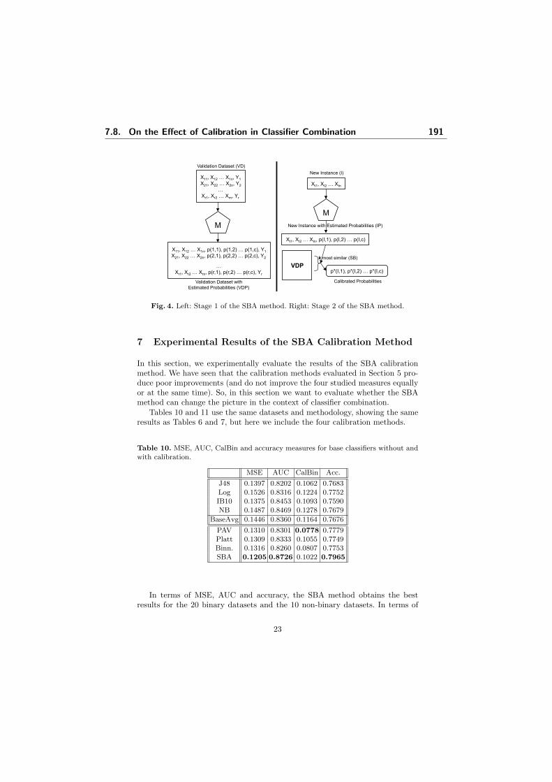
X11, X12 … X1n, p(1,1), p(1,2) … p(1,c), Y1

X21, X22 … X2n, p(2,1), p(2,2) … p(2,c), Y2

…

Xr1, Xr2 … Xrn, p(r,1), p(r,2) … p(r,c), Yr

Validation Dataset (VD)

Validation Dataset with

Estimated Probabilities (VDP)

X11, X12 … X1n, Y1

X21, X22 … X2n, Y2

…

Xr1, Xr2 … Xrn, Yr

Calibrated Probabilities

New Instance with Estimated Probabilities (IP)

VDP

p*(I,1), p*(I,2) … p*(I,c)

k most similar (SB)

XI1, XI2 … XIn

XI1, XI2 … XIn, p(I,1), p(I,2) … p(I,c)

New Instance (I)

M

M

Fig. 4. Left: Stage 1 of the SBA method. Right: Stage 2 of the SBA method.

7 Experimental Results of the SBA Calibration Method

In this section, we experimentally evaluate the results of the SBA calibrationmethod. We have seen that the calibration methods evaluated in Section 5 pro-duce poor improvements (and do not improve the four studied measures equallyor at the same time). So, in this section we want to evaluate whether the SBAmethod can change the picture in the context of classifier combination.

Tables 10 and 11 use the same datasets and methodology, showing the sameresults as Tables 6 and 7, but here we include the four calibration methods.

Table 10. MSE, AUC, CalBin and accuracy measures for base classifiers without andwith calibration.

MSE AUC CalBin Acc.

J48 0.1397 0.8202 0.1062 0.7683Log 0.1526 0.8316 0.1224 0.7752IB10 0.1375 0.8453 0.1093 0.7590NB 0.1487 0.8469 0.1278 0.7679

BaseAvg 0.1446 0.8360 0.1164 0.7676

PAV 0.1310 0.8301 0.0778 0.7779Platt 0.1309 0.8333 0.1055 0.7749Binn. 0.1316 0.8260 0.0807 0.7753SBA 0.1205 0.8726 0.1022 0.7965

In terms of MSE, AUC and accuracy, the SBA method obtains the bestresults for the 20 binary datasets and the 10 non-binary datasets. In terms of

23


Table 11. MSE, AUC, CalBin and accuracy measures for base classifiers without andwith calibration, with one random classifier.

MSE AUC CalBin Acc.

J48 0.1397 0.8202 0.1062 0.7683Log 0.1526 0.8316 0.1224 0.7752IB10 0.1375 0.8453 0.1093 0.7590NB 0.1487 0.8469 0.1278 0.7679

Random 0.4676 0.5009 0.4398 0.4317

BaseAvg 0.2092 0.7690 0.1811 0.7004

PAV 0.1568 0.7642 0.0966 0.7086Platt 0.1499 0.7665 0.0982 0.7223Binn. 0.1568 0.7610 0.0979 0.7066SBA 0.1264 0.8648 0.1080 0.7841

CalBin, the calibration method that obtains the best results is the PAV method.The results in bold mean that the differences are statistically significant.

The problem of non-monotonicity is that the more transformations we do,the more overfitting may occur, and, more importantly, the correlation betweenthe classifiers may increase (loss of diversity). We calculated Pearson’s correla-tion coefficient for the base classifiers before and after calibrating them with thethree traditional calibration techniques and SBA. While the traditional calibra-tion techniques showed no significant increase in correlation, this was effectivelyhigher for SBA. A higher correlation is, in theory, worse (less diversity), unlessthere is a general increase in classifier quality (when classifiers get better thenthey necessarily must correlate more). This latter situation seems to be moreconsistent here, as the results for AUC are much better. Nonetheless, a morethorough analysis on the relation between non-monotonic calibration and clas-sifier diversity should be done. In what follows, we will focus on whether theoverall results are better, since many factors counter-balance here.

Next, we study the effect of combination, calibration+combination, combi-nation+calibration and calibration+combination+ calibration in Table 12 withthe SBA calibration method. We compare these results with the results in Tables6, 7, 8 and 9, using the Friedman test.

This table shows that SBA gives the best results in terms of AUC. Theimprovement is now much higher than it was for the other methods. The optionsof using WCGINI or WCIMSE are not significant, but they are still better thanother weighting options (not shown in the table). The layouts with the bestresults in terms of AUC are SBA + WCIMSE and SBA + WCIMSE + Platt.The difference between these results and the rest of the results in Table 12 andTable 8 are statistically significant according to the Friedman test. Otherwise,the difference between the result of the layout SBA + WCIMSE + Platt andPAV+WCIMSE (the best result in Table 8), in terms of MSE, is not statisticallysignificant. The difference between the result of the layout SBA + WCIMSE +PAV and PAV + WCIMSE + PAV (the best result in Table 9), in terms of

24


Table 12. CombMet, CalMet+CombMet, CombMet+CalMet and Cal-Met+CombMet+CalMet results, with 1 random classifier. ∗: difference non significantrespect PAV+WCIMSE+PAV. ?: difference non significant respect PAV+WCIMSE.•: difference non significant respect PAV+WCIMSE and Binn.+WCIMSE.

MSE AUC CalBin Acc.

SBA+WCGINI 0.1145 0.8841 0.1124 0.8079SBA+WCIMSE 0.1120 0.8846 0.1056 0.8104

WCGINI+SBA 0.1147 0.8781 0.0996 0.8081WCIMSE+SBA 0.1141 0.8762 0.0975 0.8078

PAV+WCGINI+SBA 0.1123 0.8789 0.0969 0.8103Platt+WCGINI+SBA 0.1131 0.8786 0.0978 0.8101Binn.+WCGINI+SBA 0.1128 0.8777 0.0971 0.8086

PAV+WCIMSE+SBA 0.1100 0.8782 0.0933 0.8128Platt+WCIMSE+SBA 0.1111 0.8781 0.0949 0.8119Binn.+WCIMSE+SBA 0.1112 0.8765 0.0947 0.8108

SBA+WCGINI+PAV 0.1093 0.8732 0.0680 0.8161SBA+WCGINI+Platt 0.1076 0.8842 0.1031 0.8185SBA+WCGINI+Binn. 0.1135 0.8618 0.0734 0.8089SBA+WCGINI+SBA 0.1149 0.8794 0.1021 0.8068

SBA+WCIMSE+PAV 0.1085 0.8732 0.0675∗ 0.8172SBA+WCIMSE+Platt 0.1066? 0.8846 0.1023 0.8198•SBA+WCIMSE+Binn. 0.1128 0.8620 0.0728 0.8106SBA+WCIMSE+SBA 0.1140 0.8792 0.1002 0.8082

CalBin, is not statistically significant. And finally, the difference between theresult of the layout SBA + WCIMSE + Platt, PAV + WCIMSE and Binn +WCIMSE (the best results in Table 8), in terms of accuracy, is not statisticallysignificant.

In addition, we see again that the use of weights is compatible with this cali-bration method. Consequently, calibration and weighting for a wide range (mono-tonic or not) of calibration methods (even using the same validation dataset) isnot only compatible but also beneficial.

8 Discussion and Conclusions

In general terms, we now have a better understanding of classifier combinationusing probabilities. The separability and location of the probability distributionsis the key issue in understanding how classifier combination works. Measures suchas AUC, MSE and CalBin are very useful in distinguishing these separability andlocation parameters.

Apart from all these findings, it is also worth considering whether the newweighting methods, layouts, and calibration methods are able to improve thestate-of-the-art in classifier combination using probabilities. There is definitely

25


a relevant increase in the quality of the combined models over the techniqueswith traditional weighting.

In order to give a clearer picture of the overall improvement, Table 13 sum-marises this evolution of results.

Table 13. Summary of Results (using 4 models + random classifier). Each result is accompaniedwith some letters. For each column (MSE, AUC, CalBin, and accuracy measures) we have donea significant statistical test between the rows with the same letter. If the difference between themethods with the same letter is significant, we have put the letter of the best result in bold; and iftwo or more methods are better than the rest, but the difference between them is not significant, wehave underlined the letters of these methods.

MSE AUC CalBin Acc.

Base 0.2092 a 0.7690 a 0.1811 a 0.7004 aWCUnif 0.1298 a, b, d, e 0.8520 a, b, d, e 0.1337 a, b, d, e 0.7932 a, b, d, eWCAcc 0.1196 b, c, d, e 0.8630 b, c, d, e 0.1175 b, c, d, e 0.8035 b, c, d, e

WCGINI 0.1141 c,d, e, f, g0.8729 c, d, e, f, g0.1048 c,d, e, f, g0.8077 c, d, e, f, gPlatt+WCUnif 0.1294 d, f 0.8745 d, f 0.1589 d, f 0.8063 d, fPlatt+WCGINI 0.1173 e, f 0.8779 e, f 0.1293 e, f 0.8129 e, f

Platt+WCGINI+Platt 0.1091 f , g 0.8772 f, g 0.1005 f , g 0.8158 f , g

SBA+WCGINI 0.1145 g 0.8841 g 0.1124 g 0.8079 gSBA+WCGINI+SBA 0.1149 g 0.8794 g 0.1021 g 0.8068 gSBA+WCGINI+PAV 0.1093 g 0.8732 g 0.0680 g 0.8161 gSBA+WCGINI+Platt 0.1076 g 0.8842 g 0.1031 g 0.8185 g

Firstly, the WCUnif layout shows an unweighted combination of the baseclassifiers (including one random classifier). There is a clear improvement in allthe parameters over the average of the base classifiers (Base). This is significantlybetter if we use a weighted combination using a classical combination accuracy(WCAcc). Up to this point, this is a state-of-the-art solution. If we modify theweighting function to GINI (WCGINI), we get a significant improvement overWCAcc.

Secondly, the use of a traditional (monotonic) calibration method (Platt’s)is able to improve the results (both for the unweighted case and for the weightedcase using WCGINI). Nonetheless, as discussed in previous sections: using cali-bration before combination typically yields better (but uncalibrated) combina-tions, and the improvement is not applicable to MSE or CalBin. However, thiscan be easily sorted out by also using a postcalibration (layout: Platt + WCGINI+ Platt).

Thirdly, the SBA calibration method is able to get further improvement,especially in terms of AUC. The layout SBA+WCGINI excels in AUC. Again,if we are interested in a calibrated combination or in good accuracy, we can usethe layout SBA+WCGINI+PAV, which gives the best results in terms of MSEand CalBin (AUC is worse for this layout because PAV is not strictly monotonicand makes ties that may reduce the AUC). For accuracy, SBA+WCGINI+Plattseems a better option, while keeping AUC at its best.

As final recommendations, we think that classifiers that are seen as proba-bilistic estimators (and virtually any classifier can be converted into a probabilityestimator) give a more complete view of their behaviour, allowing for a more de-

26


tailed combination, using their own reliabilities. The notions of diversity andquality become more complex than for crisp (non-probabilistic), but this extracomplexity can pay off with an increase in the performance of the combinedmodel. Performance should be evaluated with several data metrics, but separa-bility (measured in terms of AUC) is a good reference, since it is insensitive tomiscalibration. Pursuing a combined model with good AUC makes sense sincewe know that we can calibrate a classifier with good AUC and get good accuracyresults from these calibrated probabilities, using the by default thresholds (e.g.0.5 for binary datasets).

From all these results and analyses, we would like to highlight some clearmessages, as follows:

– Calibration is beneficial before combination as the experimental results show,in general. Monotonic calibration methods have a more limited influencethan non-monotonic ones.

– The combination of classifiers does not typically give a calibrated result, aswe have shown by analysing the probability distributions using truncatednormal models for them. This has been confirmed by the experimental re-sults.

– We advocate for AUC as the right measure to evaluate combination perfor-mance, precisely because the combination is generally uncalibrated.

– We recommend calibration after combination, if we are interested in goodresults in terms of MSE or in terms of accuracy.

– Weighted combination is compatible with probabilities even when we usecalibration with the same dataset from which we derive the weights. Thishas been shown by the experiments. Therefore, the “double-weighting” isnot really a problem, or at least it is counteracted by other benefits.

– The weighting methods which are best when using probabilities are GINIand IMSE, even in conjunction with calibration.

– SBA, the non-monotonic calibration method, is better for combination ac-cording to the experimental results.

This better understanding of classifier combination using probabilities is not onlyuseful for the general case, but for specific applications and problems. We nowhave tools to analyse how classifiers change with calibration and combination.The distribution plots we used in section 4 can be used to analyse how calibrationand combination works with a specific set of classifiers. The use of several metrics(such as AUC, MSE, accuracy, and CalBin) are a requirement to understandwhat is really going on when classifiers are transformed and combined.

Finally, we have also raised many new questions. More elaborate tools couldbe used to analyse probability distributions theoretically, especially to addressthe general multiclass case. The use of other diversity measures, such as Spear-man’s rank correlation would also be insightful. Empirical results can also beextended with more layouts, different settings, datasets sizes and features, modeltypes, etc. In the end, calibration is a complex phenomenon by itself, which be-comes even more convoluted when coupled with the already multifarious area ofmodel combination.

27


References

1. Takeshi Amemiya. Regression Analysis when the Dependent Variable Is TruncatedNormal. Econometrica, 41(6):997–1016, 1973.

2. Miriam Ayer, H.D. Brunk, G.M. Ewing, W.T. Reid, and Edward Silverman. Anempirical distribution function for sampling with incomplete information. Annalsof Mathematical Statistics, 5:641–647, 1955.

3. A. Bella, C. Ferri, J. Hernandez-Orallo, and M.J. Ramirez-Quintana. Calibra-tion of machine learning models. In Handbook of Research on Machine LearningApplications, pages 128–146. IGI Global, 2009.

4. A. Bella, C. Ferri, J. Hernandez-Orallo, and M.J. Ramırez-Quintana. Similarity-Binning Averaging: A Generalisation of Binning Calibration. In Intelligent DataEngineering and Automated Learning - IDEAL 2009, volume 5788 of Lecture Notesin Computer Science, pages 341–349. Springer Berlin / Heidelberg, 2009.

5. Paul N. Bennett. Building Reliable Metaclassifiers for Text Learning. PhD thesis,Carnegie Mellon University, 2006.

6. Paul N. Bennett, Susan T. Dumais, and Eric Horvitz. The Combination of TextClassifiers Using Reliability Indicators. Information Retrieval, 8(1):67–98, 2005.

7. C.L. Blake and C.J. Merz. UCI repository of machine learning databases, 1998.8. Leo Breiman. Bagging predictors. Machine Learning, 24:123–140, August 1996.9. Niko Brummer. Measuring, refining and calibrating speaker and language informa-

tion extracted from speech. PhD thesis, University of Stellenbosch, 2010.10. Rich Caruana, Art Munson, and Alexandru N. Mizil. Getting the Most Out of En-

semble Selection. In ICDM ’06: Proceedings of the Sixth International Conferenceon Data Mining, pages 828–833, Washington, DC, USA, 2006. IEEE ComputerSociety.

11. Rich Caruana and Alexandru Niculescu-Mizil. Data mining in metric space: anempirical analysis of supervised learning performance criteria. In Proceedings ofthe tenth ACM SIGKDD international conference on Knowledge discovery anddata mining, KDD ’04, pages 69–78, New York, NY, USA, 2004. ACM.

12. Janez Demsar. Statistical comparisons of classifiers over multiple data sets. Journalof Machine Learning Research, 7:1–30, December 2006.

13. Thomas G. Dietterich. Ensemble methods in machine learning. In Proceedings ofthe First International Workshop on Multiple Classifier Systems, MCS ’00, pages1–15, London, UK, 2000. Springer-Verlag.

14. Thomas G. Dietterich. An experimental comparison of three methods for construct-ing ensembles of decision trees: Bagging, boosting, and randomization. MachineLearning, 40:139–157, August 2000.

15. C. Ferri, J. Hernandez-Orallo, and R. Modroiu. An experimental comparison ofperformance measures for classification. Pattern Recognition Letters, 30:27–38,January 2009.

16. C. Ferri, J. Hernandez-orallo, and M.A. Salido. Volume under the roc surface formulti-class problems. Exact computation and evaluation of approximations. InProceedings of 14th European Conference on Machine Learning, pages 108–120,2003.

17. Cesar Ferri, Peter Flach, and Jose Hernandez-Orallo. Delegating classifiers. InProceedings of the twenty-first international conference on Machine learning, ICML’04, pages 37–45, New York, NY, USA, 2004. ACM.

18. P. Flach, H. Blockeel, C. Ferri, J. Hernandez-Orallo, and J. Struyf. Decision sup-port for data mining: An introduction to ROC analysis and its applications. In

28


Data Mining and Decision Support: Integration and Collaboration, pages 81–90.Kluwer Academic Publishers, Boston, 2003.

19. Yoav Freund and Robert E. Schapire. Experiments with a New Boosting Algo-rithm. In International Conference on Machine Learning, pages 148–156, 1996.

20. Joao Gama and Pavel Brazdil. Cascade generalization. Machine Learning, 41:315–343, December 2000.

21. Ursula Garczarek. Classification Rules in Standardized Partition Spaces. PhDthesis, Universitat Dortmund, 2002.

22. Martin Gebel. Multivariate calibration of classifier scores into the probability space.PhD thesis, University of Dortmund, 2009.

23. David J. Hand and Robert J. Till. A simple generalisation of the area under theroc curve for multiple class classification problems. Machine Learning, 45:171–186,October 2001.

24. Jennifer A. Hoeting, David Madigan, Adrian E. Raftery, and Chris T. Volinsky.Bayesian model averaging: A tutorial. Statistical Science, 14(4):382–417, 1999.

25. Ludmila I. Kuncheva. A theoretical study on six classifier fusion strategies. IEEETransactions on Pattern Analysis and Machine Intelligence, 24:281–286, February2002.

26. Ludmila I. Kuncheva. Combining Pattern Classifiers: Methods and Algorithms.Wiley-Interscience, 2004.

27. Ludmila I. Kuncheva. Diversity in multiple classifier systems. Information Fusion,6(1):3 – 4, 2005. Diversity in Multiple Classifier Systems.

28. Ludmila I. Kuncheva and Christopher J. Whitaker. Measures of diversity in classi-fier ensembles and their relationship with the ensemble accuracy. Machine Learn-ing, 51:181–207, May 2003.

29. A. H. Murphy. Scalar and vector partitions of the probability score: Part II. n-statesituation. Journal of Applied Meteorology, 11:1182–1192, 1972.

30. John C. Platt. Probabilistic outputs for support vector machines and comparisonsto regularized likelihood methods. In Advances in Large Margin Classifiers, pages61–74. MIT Press, Boston, 1999.

31. Adrian E. Raftery, Tilmann Gneiting, Fadoua Balabdaoui, and Michael Po-lakowski. Using bayesian model averaging to calibrate forecast ensembles. monthlyweather review 133, 2005.

32. Ryan Rifkin and Aldebaro Klautau. In defense of one-vs-all classification. Journalof Machine Learning Research, 5:101–141, December 2004.

33. Tim Robertson, F. T. Wright, and R. L. Dykstra. Order Restricted StatisticalInference. John Wiley & Sons, 1988.

34. Sergey Tulyakov, Stefan Jaeger, Venu Govindaraju, and David Doermann. Reviewof classifier combination methods. In Hiromichi Fujisawa Simone Marinai, editor,Studies in Computational Intelligence: Machine Learning in Document Analysisand Recognition, pages 361–386. Springer, 2008.

35. Ian H. Witten and Eibe Frank. Data mining: practical machine learning tools andtechniques with java implementations. SIGMOD Record, 31:76–77, March 2002.

36. David H. Wolpert. Stacked generalization. Neural Networks, 5:241–259, 1992.37. Bianca Zadrozny and Charles Elkan. Transforming classifier scores into accurate

multiclass probability estimates. In Proceedings of the eighth ACM SIGKDD in-ternational conference on Knowledge discovery and data mining, KDD ’02, pages694–699, New York, NY, USA, 2002. ACM.

29


model integration in data mining: from local to global...

Documents