model-free tests for genetic linkage unit 1 · pdf file · 2017-08-27when...

FOR

REVIEW

ONLY

UNIT 1.8Model-Free Tests for Genetic LinkageChristopher I. Amos,1 Audrey Schnell,2 Wei V. Chen,1 and Robert C. Elston3

1University of Texas, M.D. Anderson Cancer Center, Houston, Texas2University of Washington, Seattle, Washington3Case Western University, Cleveland, Ohio

ABSTRACT

This unit covers statistical methods of linkage analysis that do not require the assumptionof a detailed genetic model, as is required for standard lod score analysis. The unithas been updated to include the latest methods in sib-pair analysis, including updatesto using the software program SIBPAL as well as the relative-pair analysis softwareapplications GENEHUNTER, GENEHUNTER PLUS, and Merlin. Curr. Protoc. Hum.Genet. 75:1.8.1-1.8.32. C© 2012 by John Wiley & Sons, Inc.

Keywords: robust linkage tests � pedigree methods � sib pair tests

INTRODUCTION

This unit discusses the application of several model-free genetic linkage tests (alsosee Key Concepts). Model-free procedures for evaluating linkage are generally appliedwhen investigating diseases and traits for which simple Mendelian inheritance patternsare not observed. Model-free procedures should be used to provide either a preliminaryevaluation of the data for linkage or confirmatory analyses when results obtained by theusual lod score approach are unclear (see UNITS 1.4 & 1.7 for discussion of lod scores).

Examples illustrating the application of several model-free linkage methods are providedlater in this unit (see Strategic Approach). Example 1 describes three simple methodsfor testing linkage via the affected-sib-pair (ASP) method without the use of computersoftware. Example 2 describes linkage analysis of sib-pair data with the aid of thecomputer programs GENIBD and SIBPAL. The SIBPAL module, which is part of theStatistical Analysis for Genetic Epidemiology (S.A.G.E.) package of programs, includesan affected-sib-pair (ASP) method (i.e., the mean test; also see Example 1) as well asanother technique based on sib-pair analysis, the Haseman-Elston (H-E) method, whichalso uses information from unaffected pairs; therefore, SIBPAL has been chosen as theexample of a sib-pair analysis program in this unit. The ASP test compares the similarityof marker alleles shared between sib pairs to that predicted on the basis of randomsegregation. The H-E method compares similarity of marker alleles shared among sibpairs to sib-pair dissimilarity of disease status or quantitative trait values. Example 3applies a model-free test for genetic linkage using GENEHUNTER PLUS. Example 4describes analysis allowing for SNPs that are in strong linkage disequilibrium, usingMERLIN. Because correct inferences from genetic linkage tests require correct marker-allele frequencies, care must be taken to ensure that the marker alleles used in the analysisare well specified and that the frequencies are well estimated. The Strategic Approachsection therefore includes methods for estimating allele frequencies, either from unrelatedindividuals (Support Method 1) or from the pedigrees that have been selected for study(Support Method 2).

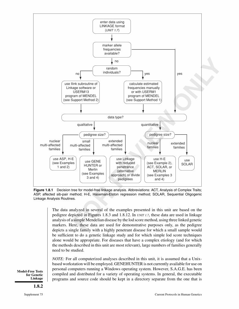
Methods for studying quantitative traits are not discussed in detail in this unit, but theprocedures outlined for the H-E test (see Example 2) can be applied to either quantitativeor qualitative data. Figure 1.8.1 provides a decision tree outlining the choice of methodsfor analysis covered in this unit.

Current Protocols in Human Genetics 1.8.1-1.8.32, October 2012Published online October 2012 in Wiley Online Library (wileyonlinelibrary.com).DOI: 10.1002/0471142905.hg0108s75Copyright C© 2012 John Wiley & Sons, Inc.

GeneticMapping

1.8.1

Supplement 75

FOR

REVIEW

ONLY

Model-Free Testsfor Genetic

Linkage

1.8.2

Supplement 75 Current Protocols in Human Genetics

enter data usingLINKAGE format

(UNIT 1.7)

marker allelefrequenciesavailable?

randomindividuals? yes

no

yesno

use Ilink subroutine ofLinkage software or

USERM13program of MENDEL

(see Support Method 2)

calculate estimatedfrequencies manually

or with USERM1program of MENDEL

(see Support Method 1)

data type?

qualitative quantitative

pedigree size? pedigree size?

nuclearmulti-affected

families

extendedmulti-affected

families

smallmulti-affected

families

nuclearfamilies

extendedfamilies

use ASP, H-E(see Examples

1 and 2)

use GENEHUNTER or

Merlin(see Examples

3 and 4)

use Linkagewith reducedpenetrance(alternative

approach) or dividepedigrees

use H-E(see Example 2),ACT, SOLAR, or

MERLIN(see Examples 3

and 4)

useSOLAR

Figure 1.8.1 Decision tree for model-free linkage analysis. Abbreviations: ACT, Analysis of Complex Traits;ASP, affected sib-pair method; H-E, Haseman-Elston regression method; SOLAR, Sequential OligogenicLinkage Analysis Routines.

The data analyzed in several of the examples presented in this unit are based on thepedigree depicted in Figures 1.8.3 and 1.8.12. In UNIT 1.7, these data are used in linkageanalysis of a simple Mendelian disease by the lod score method, using three linked geneticmarkers. Here, these data are used for demonstrative purposes only, as the pedigreedepicts a single family with a highly penetrant disease for which a small sample wouldbe sufficient to do a genetic linkage study and for which simple lod score techniquesalone would be appropriate. For diseases that have a complex etiology (and for whichthe methods described in this unit are most relevant), large numbers of families generallyneed to be studied.

NOTE: For all computerized analyses described in this unit, it is assumed that a Unix-based workstation will be employed. GENEHUNTER is not currently available for use onpersonal computers running a Windows operating system. However, S.A.G.E. has beencompiled and distributed for a variety of operating systems. In general, the executableprograms and source code should be kept in a directory separate from the one that is

FOR

REVIEW

ONLY

GeneticMapping

1.8.3

Current Protocols in Human Genetics Supplement 75

used for analysis. A softlink to the area in which the executable programs are kept can becreated by typing ln -s [executable filename], or the systems administratorcan store the executable programs in the bin directory, where they can be used by anyonewithout requiring softlinks.

KEY CONCEPTS

Model-Dependent Versus Model-Free Versus Nonparametric Tests

The usual likelihood-based approaches for genetic linkage analysis (UNIT 1.4) requirethat a correct model be specified for the relationship between an individual’s genotypeand the corresponding chance of displaying a disease or other trait phenotype. In thecommonly used lod score approach to obtaining evidence for linkage, the log10 of thelikelihood for the data is calculated assuming a particular genetic model and a particularrecombination fraction between the marker locus and disease locus. This is comparedwith the log10 for the likelihood of the data assuming the same genetic model, butwith the recombination fraction between the marker and disease loci set to 50%. Thisapproach assumes that the correct genetic model is known, i.e., that the number of allelesinfluencing disease susceptibility, the penetrance of each of corresponding genotypes,and the allele frequencies are correctly specified. Model-free methods, e.g., the affected-sib-pair method, do not require that the genetic model explaining disease inheritance beexplicitly specified. Nonparametric or robust procedures further relax any assumptionabout the underlying statistical distributions used to determine significance. To avoidassumptions about the statistical distribution of the derived test statistic, simulationstudies can be performed to develop a nonparametric and model-free statistical test forlinkage. Correctly simulating data to represent the correlation structure present in geneticstudies can be challenging. As an alternative, one can use the observed data and permuteit, resampling the actual data that are available for study in a manner that will allowrandom shuffling of the outcome data that pertain to the test of the null hypothesis whilepreserving the correlation structure among markers or other predictors.

Identity ?in?by? State and Identity by Descent

Whenever a pair of individuals shares the same allele at a locus, that allele is saidto be identical ?in?by? state (IBS). If the individuals have inherited that same allelefrom some common ancestor, the allele is also identical by descent (IBD). Because ofMendelian inheritance, an average of 1/4 of sib pairs will share two alleles IBD, 1/2 willshare one allele IBD, and 1/4 will share no alleles IBD. To avoid confusion, in this unitthe term IBD has been reserved for results obtained from analysis of a specific genomicregion. The average proportion of autosomal genetic material shared between any pair ofrelatives is called the kinship coefficient (κ). The kinship coefficient for non-inbred pairsof individuals is (1/2)R+1, where R is the degree of relationship between the pair, e.g., forfirst-degree relatives, R = 1 and κ = 1/4; for second-degree relatives, R = 2 and κ = 1/8.

IBD information is often summarized in terms of the proportion of alleles that a dataset of pairs of individuals shares IBD; this proportion is indicated as π. Typically, thisproportion must be estimated from the data, and the estimate of π is usually denotedby π . This estimate is derived by calculating the sum of the probability that the pairshares two alleles IBD plus 0.5 times the probability that the pair shares one allele IBD.Figure 1.8.2 shows the pedigree of a sample family with alleles indicated. Table 1.8.1lists the number of alleles shared IBS and IBD for some of the pairs of individuals in thatpedigree. It is assumed that the locus under study has only four alleles. Usually, singlenucleotide polymorphisms that are typically genotyped on high-dimensional microarraysare diallelic, which limits the information available from a single locus, but with thedecreased costs of genotyping, multiple loci can be jointly queried.

FOR

REVIEW

ONLY


Linkage

1.8.4


Table 1.8.1 Alleles Shared IBD and IBS for Some Pairs of Individuals in Figure 1.8.2

Number of alleles shared

Pair IBS IBDProportion of alleles

shared IBD (π)Kinship

coefficient

6-7 1 1 0.5 0.25

5-6 1 0 0 0.125

3-4 1 0 0 0

21 3

3 14 2

4 5 6 7

1 3 1 3 1 4 1 3

Figure 1.8.2 Sample pedigree for illustrating identity by descent and identity in state calculations.The box with the slash represents a deceased individual.

In the sample pedigree depicted in Figure 1.8.2, it is evident that individuals 6 and 7 haveinherited the same “1” allele from their father but different alleles from their mother;hence, they share one allele IBD and IBS. Although individuals 5 and 6 both have a“1” allele, this allele was not present in their common mother, individual 2; therefore,this allele “1” cannot have been inherited from the same common ancestor. Similarly,individuals 3 and 4 have a common “1” allele but have no shared ancestors. In bothcases, the “1” allele is IBS but not IBD. Calculating the proportion of alleles IBD forindividuals 4 and 5 is more complicated. It is obvious that a “1” allele must have beentransmitted from deceased individual 1, but the entire genotype for individual 1 cannotbe deduced; it could have been 1/1, 1/2, 1/3, or 1/4. Therefore, it is necessary to performprobability calculations that sum the probability of each of these possible genotypes, asdescribed in Amos et al. (1990a). To calculate the proportion of alleles shared IBD forindividuals 4 and 5, let pij represent the probability of genotype ij in the population fromwhich this pedigree was sampled (with i and j each representing one of the alleles 1,2, 3, and 4). Then, the estimate of proportion of alleles shared IBD (π ) is calculated asfollows:

11 12 13 14

11 12 13 14

3 1( )

16 16ˆ1 1

( )4 16

p p p p

p p p pπ =

+

+ ++

+ +

FOR

REVIEW

ONLY

GeneticMapping

1.8.5


The type of tedious calculation shown above is automated as a part of the SIBPAL orGENEHUNTER procedures (see Strategic Approach). As mentioned above, π dependsupon estimates of genotype frequency whenever there are parents for whom genotypedata are missing. Tests based upon IBD sharing for pairs of relatives are more powerfulthan tests based upon IBS sharing, unless the marker under consideration is extremelyinformative (i.e., has high heterozygosity; see UNIT 1.4), but programs such as ERPA (Curtisand Sham, 1994) for calculating IBD in extended pedigrees can be computationallydemanding.

In a pedigree, individuals who have studied descendants but whose parents have not beenstudied are called founding parents. Individuals marrying into the pedigree who are notaffected with the disease being studied are one class of founding parents (often calledmarry-ins). In the sample pedigree shown in Figure 1.8.2, the founding parents are 1, 2,and 3.

Statistical Terms: Mean, Variance, Skewness, and Kurtosis

Four measures characterizing a distribution of values are used in this unit. Letting xi

represent the value of the ith observation with i varying from 1 to n, the mean (x) isdefined as:

1

1 n

ii

x xn

The usual estimator of the variance (σ 2) is defined as:

2 2

1

1ˆ ( *)

1

n

ii

xn

where xi* represents xi – x . Variance is a measure of the spread of values about thecommon mean. The standard deviation is the square root of the variance.

The skewness is calculated by an equation analogous to that for variance, except that xi*is cubed rather than squared, and then divided by the cube of the standard deviation. Fora normal distribution, the skewness is 0, indicating that the distribution is symmetricalabout its mean. Positive skewness suggests that most values are clustered at the low endof the distribution but the remaining values tend to be relatively high.

The kurtosis is also calculated by an equation analogous to the one for variance, but xi* israised to the fourth power and divided by the fourth power of the standard deviation, andthe value 3 is then subtracted. Kurtosis reflects the flatness or peakedness of the curve ofdistribution relative to the normal distribution, for which the coefficient of kurtosis is 3.

Hypothesis Testing

Linkage analysis generally compares two competing hypotheses—that of linkage and thatof no linkage. This is done by means of a hypothesis test, which contrast two statementsabout a set of data, e.g., a null hypothesis (of no linkage) and an alternate hypothesis(of linkage). The null hypothesis is constructed by generating a statistic in which someof the parameters that are used to characterize the data are constrained to particularvalues. The alternate hypothesis is constructed using a broader set of constraints on the

FOR

REVIEW

ONLY


Linkage

1.8.6


parameters that characterize the data than those used to construct the null hypothesis,so that the alternate hypothesis includes the null hypothesis as a possibility. A simplealternate hypothesis can be postulated in which the parameters that were constrained toa particular value under the null hypothesis are constrained to an alternative value underthe alternate hypothesis. For example, it is possible to test a null hypothesis in which themean of a distribution is 0 against a simple alternate hypothesis that the mean is –1.0, oragainst a one-sided alternate hypothesis in which the mean of the distribution is ≤0, oragainst the two-sided alternate hypothesis that the mean is any value. The significancelevel of a hypothesis test is the probability of rejecting the null hypothesis given that it isactually true, i.e., the probability of making a false judgment against the null hypothesis.The power of a hypothesis test is the probability of correctly rejecting the null hypothesisgiven that a simple alternate hypothesis is true. For a more detailed description of theseterms, a standard reference such as Rosner (1982) should be consulted.

Hypothesis tests are constructed by developing a test statistic for evaluating a specificnull hypothesis, then comparing this statistic to a reference distribution that would begenerated from similar data based on the assumption that the null hypothesis is true. Thesignificance of the test statistic is assessed by comparing the observed value to the valuesprovided by the reference distribution, and represents the probability of having obtainedthe observed test statistic (or one that is more extreme) if the null hypothesis were true. Inmany cases, a suitable reference distribution for assessing significance can be obtainedfrom theoretical calculations. For the cases discussed in this unit, the reference distribu-tions are either the normal or the χ2 distribution, for which any standard statistics textor book of mathematical tables can be consulted. Standard statistical software packages,e.g., Statistical Analysis System (SAS; available from SAS Institute), can also be used toassess significance. Simulation studies may be useful for assessing significance in somecases, e.g., where the distribution of a test statistic is not known, making it impossibleto choose an appropriate reference distribution. In such cases, data are simulated underthe null hypothesis and the observed test statistic is compared to that obtained fromthe simulated data. The significance will then be the proportion of replicates from thesimulation with values equal to or greater than the observed test statistic.

Occasionally, in the study of diseases having complex etiology, only a single hypothesiswill be tested; in this case, assessing the significance is straightforward. Usually, however,multiple hypothesis tests are performed; here, the probability that the results of anyof the tests will be significant increases with the number of tests. To control for theoverall probability of a false-positive finding in multiple hypothesis testing, correctionprocedures are needed. The easiest procedure to apply is Bonferroni’s correction, inwhich the observed significance value is multiplied by the number of tests. Multipletests are conducted either when testing for linkage with multiple markers or when tryingdifferent test procedures and/or genetic models in the analysis. When multiple linkedmarkers are used, the tests are not independent; hence Bonferroni’s approach is tooconservative (Feingold et al., 1993), i.e., it will result in too stringent a criterion forsignificance. Two approaches are often used to account for the multiple testing problem.When considering multiple markers, the first approach is to require a high level ofsignificance, i.e., the usual lod score criterion of 3.0 corresponds to a χ2 deviate of 13.8,which yields a significance level of <1/10,000 (Chotai, 1984). Lander and Kruglyak(1995) showed under an assumption of no interference that a lod of 3.3 provides agenome-wide significance level of 5% of finding a false positive result, given that there isno genetic factor explaining data from a family study. Under more realistic assumptionsallowing for interference, the suggested lod of 3.3 is too conservative (Sawcer et al.,1997; Morton, 1998). Alternatively, the gene identification problem can be evaluatedfrom a Bayesian framework, in which case a lod score of 3.0 corresponds to a posteriorprobability of linkage of ∼95% under most testing strategies (Ott, 1999, p. 68).

FOR

REVIEW

ONLY

GeneticMapping

1.8.7


When multiple genetic models or test procedures have been applied in the linkageanalysis, some explicit correction for multiple testing is required; Bonferroni’s correctionis a conservative approach in such cases. Simulation approaches have also been advocated(Davis et al., 1996) since they can allow for correlation among the tests and thus aremore powerful than a simple Bonferroni correction would be. Corrections for multipletesting are also required when performing association studies in which multiple allelesat a locus are being studied. Allison and Beasley (1998) developed a simulation-basedapproach to correct for multiple testing in association studies.

STRATEGIC APPROACH

Example 1: Simple Methods for Linkage Testing in Affected Sib Pairs

Three tests using IBD information are widely used for genetic linkage testing with af-fected pairs of sibs (Blackwelder and Elston, 1985). These can be carried out withoutrelying on a computer program. The mean test evaluates whether there is an excessproportion of estimated alleles shared IBD (π) among affected individuals. The propor-tion test (Suarez et al., 1978) compares, among sib pairs, the proportion sharing bothalleles IBD to 1/4, which is the proportion expected under the null hypothesis of nolinkage. The goodness-of-fit test compares the proportions of sibs sharing zero, one, ortwo alleles IBD to 1/4, 1/2, and 1/4, respectively (again, the proportions expected under thenull hypothesis). The power of each of these tests depends upon the underlying geneticmechanism involved in the disease etiology. Constructing the optimal test for linkagerequires knowledge of the genetic mechanism (Schaid and Nick, 1990), and this is notgenerally feasible a priori. However, for most alternate hypotheses, the mean test is morepowerful than the other tests. One approach, advocated by Schaid and Nick (1990), is todo both the mean and proportion tests and compare results: if the proportion test shows ahigher significance than the mean test, recessive-like inheritance is suggested. The opti-mal approach for combining data from sibships of varying sizes is unclear. Under the nullhypothesis of no linkage, there is little or no inflation of the proportion of false-positivetests with increasing sibship size (Suarez and Van Eerdewegh, 1984; Blackwelder andElston, 1985). However, under the alternate hypothesis of tight linkage, the informationcontent per sibship of size n is proportional to n – 1 (Hodge, 1984). Use of this weightingscheme generally provides slightly more powerful tests for linkage (Suarez and VanEerdewegh, 1984) at the cost of increased complexity.

For some highly polymorphic loci, e.g., the human histocompatibility leukocyte anti-gen (HLA) system and microsatellite markers, IBD sharing can often be immediatelyidentified. As an example, consider the data presented in Table 1.8.2, in which geneticlinkage between the HLA-DR locus and insulin-dependent diabetes mellitus (IDDM) isdocumented. Among the 137 affected sib pairs, 59% were observed to share two allelesIBD, 34% were observed to share one allele IBD, and 7% were observed to share noalleles IBD. Let n represent the number of affected sib pairs, f2 represent the proportionof sib pairs sharing two alleles IBD, f1 represent the proportion of sib pairs sharing oneallele IBD, and f0 represent the proportion of sib pairs sharing no alleles IBD. The meantest compares the mean proportion of alleles shared IBD among affected sib pairs to 0.5,i.e., it tests whether f2+ 1/2f1 > 0.5. Using data from Table 1.8.2, the test statistic (t2) iscalculated as follows under the variance determined by the null hypothesis:

2 2 1

2

(2 1) 2

[2(0.59) 0.34 1] 2(137) 8.61

t f f n

t

FOR

REVIEW

ONLY


Linkage

1.8.8


Table 1.8.2 IBD Sharing for the HLA System Among 137 Sib PairsAffected by Insulin-Dependent Diabetes Mellitusa,b

f2 f1 f0 Total

n 81 46 10 137

Expected ratios 1/41/2

1/4

Expected numbers 34 69 34aDefinitions: n = number of affected sib pairs; f2 = sib pairs sharing 2 alleles IBD; f1 = sibpairs sharing 1 allele IBD; f0 = sib pairs sharing 0 alleles IBD.bData from Cox and Spielman (1989).

The proportion test compares f2 to 1/4. Using data from Table 1.8.2, the test is calculatedas follows:

2

1 2

1

14

4 3

137(0.59 0.25)4 9.19

3

nt f

t

These two tests can be compared with a normal distribution provided that n > 60. Finally,a goodness-of-fit test can be constructed by comparing observed to expected numbers ofindividuals in each of the allele-sharing categories. Using the data from Table 1.8.2, thegoodness-of-fit test is constructed as follows:

2 2 22

2 1 0

2222

1 1 12 2 2

4 2 4

2(137)[2(0.59 0.25) (0.34 0.5) 2(0.07 0.25) ] 88.12

n f f f

The test statistic obtained from this equation can then be compared to a χ2 distributionhaving two degrees of freedom.

The three tests above (using the data from Table 1.8.2) all yield p values <0.0001. Theslightly more significant test statistic derived from the proportion test (9.19) as comparedto that obtained from the mean test (8.61) suggests that the effects of a locus linked to theHLA-DR locus are recessively acting. Although mathematically simple, the goodness-of-fit test is generally less powerful than the mean test and is not often used for sib-pairanalyses.

Example 2: Using SIBPAL Software to Perform Affected-Sib-Pair and RelatedAnalyses

SIBPAL, part of the S.A.G.E. package of programs (S.A.G.E., 2011), can perform severalmodel-free tests for genetic linkage of both qualitative and quantitative traits using dataon sib pairs or sibships. Tests available in SIBPAL include the mean test (Blackwelderand Elston, 1985) and Haseman–Elston (H-E) test (Haseman and Elston, 1972; Palmeret al., 2000; Shete et al., 2003); both will be illustrated here using a binary trait. SIBPALperforms the mean test and a test of the proportion of allele sharing among concordantlyaffected and unaffected sib pairs, and also for discordant sib pairs. Estimates are obtained

FOR

REVIEW

ONLY

GeneticMapping

1.8.9


for the probabilities that sibs share 0, 1, or 2 alleles IBD (f0, f1, and f2 respectively). Theexample that is being presented is from a study of the genetics of schizophrenia andincludes data from 121 families (Cubells et al., 2011).

The Haseman-Elston methodSIBPAL performs various types of H-E regression for quantitative traits. The H-E methodwas originally developed for quantitative traits, but has been adapted for use with quali-tative traits; the latter application is the focus of the description here (Wang and Elston,2005). In the original formulation of H-E, Yij may be allowed to represent the phenotype(usually a quantitative value) for the jth individual (j = 1,2) in the ith pair of sibs from apedigree (Wang and Elston, 2005). The original H-E test used the transformation Zi =(Yi1 – Yi2)2. Subsequently, the values of Zi are regressed on π i, where i indexes the sibpair. The regression coefficient for any set of pairs depends only upon the recombinationfraction and the genetic variance attributable to any putative genetic locus that is linkedto the marker being considered (Amos and Elston, 1989).

The current version of the H-E regression uses the a weighed combination of thesquared trait difference and squared mean-corrected sum, and is adjusted for the non-independence of sib-pairs and the non-independence of squared trait sums and differences(W4 option for the dependent variable) (Shete et al., 2003). In this example, we use thebest linear unbiased predictor (BLUP) of the sibship mean for mean-correcting thesquared sib-pair sum where the sibship mean is the mean of the trait values for a givensibship. The methods that use a mean-corrected sum are asymptotically more powerfulthan the original Haseman-Elston method, which is independent of the population mean(Wang and Elston, 2005; Sinha and Gray-McGuire, 2008). For a binary trait, an affectedindividual is coded 1 and an unaffected individual 0, and this is treated as a quantitativetrait.

Asymptotic p values and optionally empirical p values from the permutation distributionare reported. For empirical p values, the estimates of IBD sharing, the predictor in theregression, are permuted both within sibships and across sibships of the same size.

For binary traits with a variable age of onset, S.A.G.E. can use age-of-onset informa-tion in a model-free linkage analysis. The age-at-onset distribution is modeled on theassumption that the time to onset of disease can be described by a cumulative normaldistribution, but a power transformation can be estimated to transform the age-at-onsetdata to approximate normality. The susceptibility to disease is represented as a functionof the lifetime risk for susceptibility among individuals based on the affection statusof the parents (affected, unaffected, or unknown). Covariates can also be included. TheS.A.G.E. program AGEON obtains maximum likelihood estimates of the parameters thatdetermine “susceptibility” to disease as a function of age, producing a quantitative sus-ceptibility trait for each individual that can be used as the trait data in SIBPAL (Dawsonet al., 1990).Using the S.A.G.E. program AGEON to obtain estimates for the suscepti-bility to disease this way, and using these estimates as the trait values in SIBPAL, maylead to more power (Schnell et al., 2011).

A more detailed discussion of the theory and options is available in the SIBPAL andAGEON documentation.

Using S.A.G.E.S.A.G.E. includes a Graphical User Interface (GUI) for importing data into S.A.G.E.and creating parameter files to execute the individual programs. S.A.G.E. is very flexibleand can accommodate data in a variety of formats (Igo and Schnell, 2012). The data

FOR

REVIEW

ONLY


Linkage

1.8.10


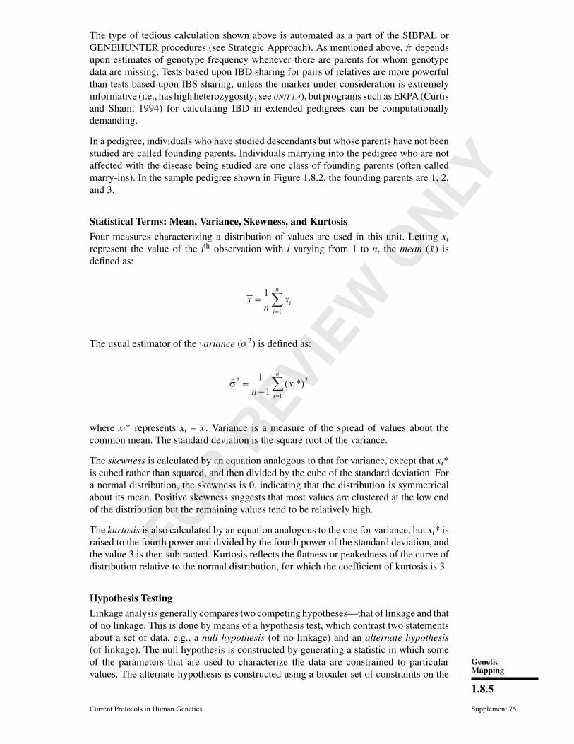
Figure 1.8.3 Dialog box for creating a new S.A.G.E. project.

can include any number of traits (quantitative or qualitative), covariates, and markersin any order. Any valid alphanumeric character can be used for missing individuals,traits, and delimiters, provided the same character is not used for more than one purpose(e.g., a missing value and column delimiter). Necessary fields to describe family dataare the Pedigree ID, Individual ID, Father, Mother, and Sex. The unique combinationof family and individual IDs provide a unique identifier for every individual. Using theGUI, variables in the data are mapped to S.A.G.E. fields via pull-down menus. Programsare available within S.A.G.E. to obtain descriptive statistics (PEDINFO), check forMendelian inconsistencies (MARKERINFO), and detect relationship errors (RELTEST).S.A.G.E. is available for Unix, PC, and Mac and can be downloaded from the Web site.Comprehensive documentation is available.

Performing an analysis using SIBPAL1. Import the data into S.A.G.E. using the GUI. We begin by creating a new project

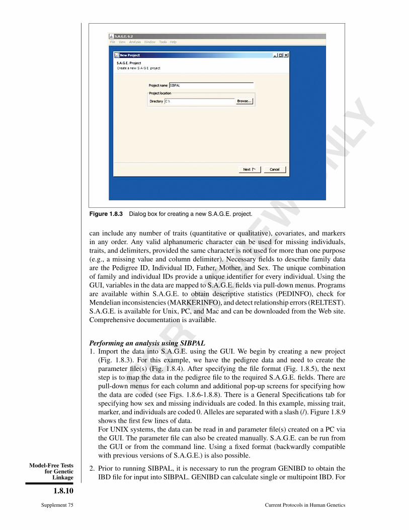
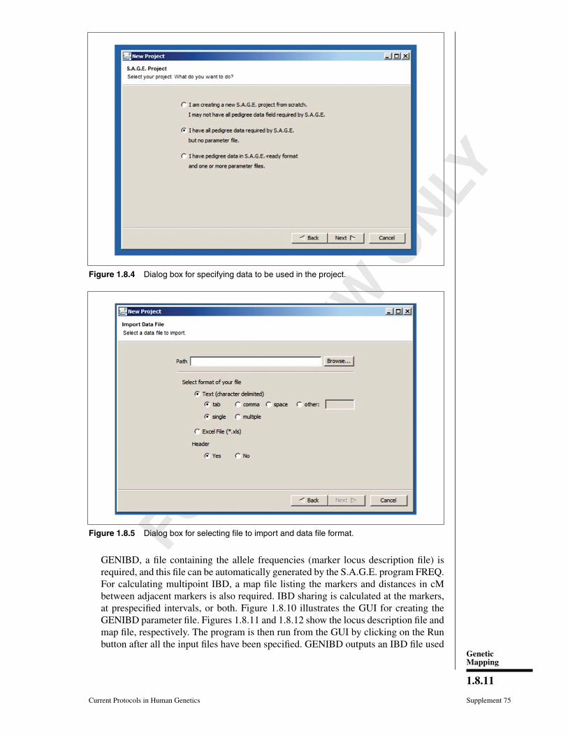
(Fig. 1.8.3). For this example, we have the pedigree data and need to create theparameter file(s) (Fig. 1.8.4). After specifying the file format (Fig. 1.8.5), the nextstep is to map the data in the pedigree file to the required S.A.G.E. fields. There arepull-down menus for each column and additional pop-up screens for specifying howthe data are coded (see Figs. 1.8.6-1.8.8). There is a General Specifications tab forspecifying how sex and missing individuals are coded. In this example, missing trait,marker, and individuals are coded 0. Alleles are separated with a slash (/). Figure 1.8.9shows the first few lines of data.For UNIX systems, the data can be read in and parameter file(s) created on a PC viathe GUI. The parameter file can also be created manually. S.A.G.E. can be run fromthe GUI or from the command line. Using a fixed format (backwardly compatiblewith previous versions of S.A.G.E.) is also possible.

2. Prior to running SIBPAL, it is necessary to run the program GENIBD to obtain theIBD file for input into SIBPAL. GENIBD can calculate single or multipoint IBD. For

FOR

REVIEW

ONLY

GeneticMapping

1.8.11


Figure 1.8.4 Dialog box for specifying data to be used in the project.

Figure 1.8.5 Dialog box for selecting file to import and data file format.

GENIBD, a file containing the allele frequencies (marker locus description file) isrequired, and this file can be automatically generated by the S.A.G.E. program FREQ.For calculating multipoint IBD, a map file listing the markers and distances in cMbetween adjacent markers is also required. IBD sharing is calculated at the markers,at prespecified intervals, or both. Figure 1.8.10 illustrates the GUI for creating theGENIBD parameter file. Figures 1.8.11 and 1.8.12 show the locus description file andmap file, respectively. The program is then run from the GUI by clicking on the Runbutton after all the input files have been specified. GENIBD outputs an IBD file used

FOR

REVIEW

ONLY


Linkage

1.8.12


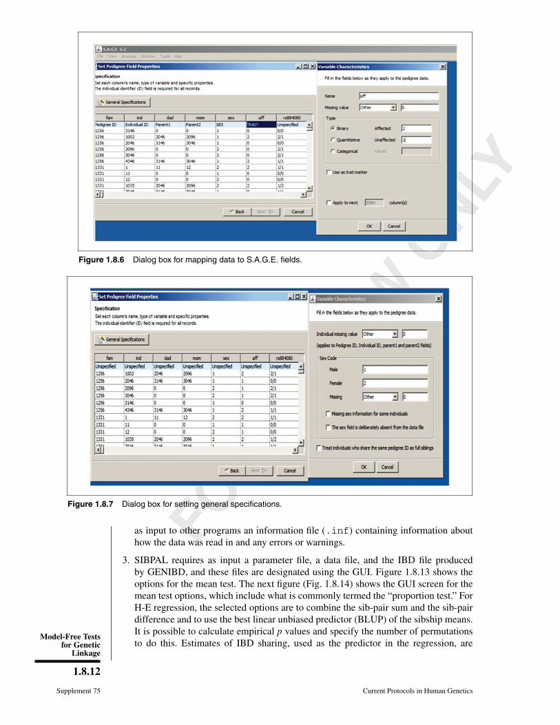
Figure 1.8.6 Dialog box for mapping data to S.A.G.E. fields.

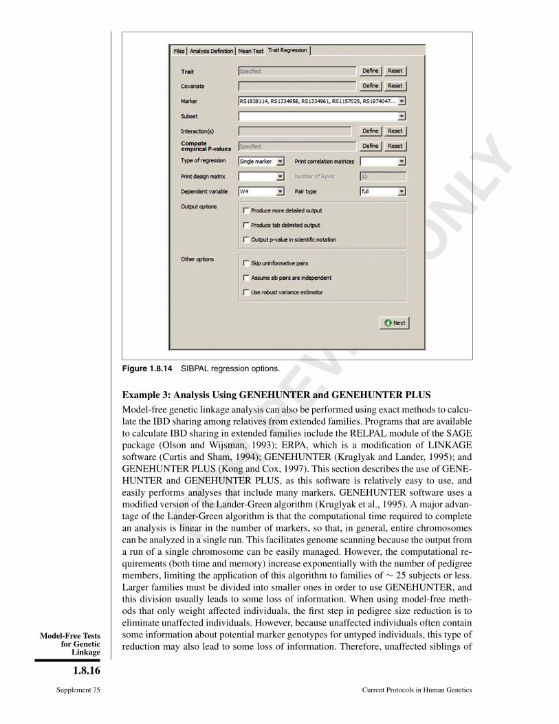
Figure 1.8.7 Dialog box for setting general specifications.

as input to other programs an information file (.inf) containing information abouthow the data was read in and any errors or warnings.

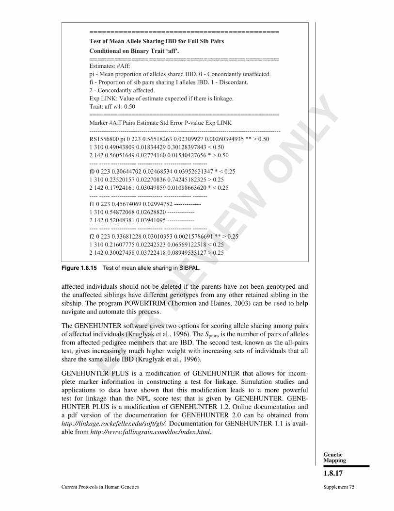
3. SIBPAL requires as input a parameter file, a data file, and the IBD file producedby GENIBD, and these files are designated using the GUI. Figure 1.8.13 shows theoptions for the mean test. The next figure (Fig. 1.8.14) shows the GUI screen for themean test options, which include what is commonly termed the “proportion test.” ForH-E regression, the selected options are to combine the sib-pair sum and the sib-pairdifference and to use the best linear unbiased predictor (BLUP) of the sibship means.It is possible to calculate empirical p values and specify the number of permutationsto do this. Estimates of IBD sharing, used as the predictor in the regression, are

FOR

REVIEW

ONLY

GeneticMapping

1.8.13


Figure 1.8.8 Dialog box for reading in markers.

Fam ind dad mom sex aff rs884080 rs2017143 rs2840531………1256 6 0 0 1 0 0/0 0/0 0/0 0 …..1256 2 2046 2096 1 2 2/1 2/2 2/2 …....

.

Figure 1.8.9 ??

permuted by SIBPAL both within sibships and across sibships of the same size toobtain empirical p values.

4. SIBPAL output. SIBPAL produces several output files. There is the .inf file, a filefor the mean test results, and a file for the regression results. Options for other filesare available, including an option for more detailed regression output.

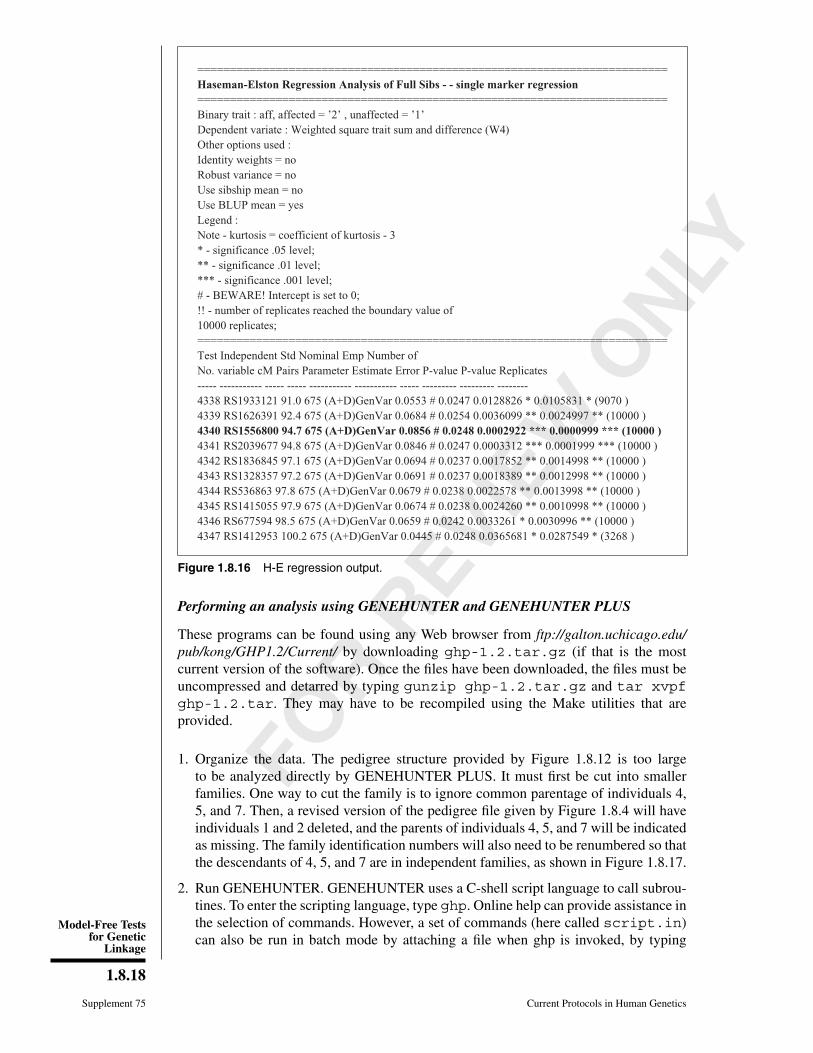
5. Interpreting the results. Figure 1.8.15 shows a sample of the Mean test output(.mean). The first section shows the legend and the next reports the mean IBDsharing (π) for sibs who are concordantly unaffected (0), discordant (1), and concor-dantly affected (2), sharing 0, 1, or 2 alleles IBD. The last column shows the expectedvalue and direction if there is linkage. For illustration, the most significant marker isshown here. For sibs sharing 0 or 2 alleles IBD, the results are significant at the 0.01(**) and 0.05 (*) level, respectively.The next section reports, for siblings sharing 0, 1, or 2 alleles IBD (f0, f1, f2), theproportion of sib pairs who are concordantly unaffected and affected (0,2), and if thatnumber is significantly different than expected. For sibs sharing 0 alleles IBD, theresults for the concordantly affected and unaffected pairs are significantly differentthan expected (p < 0.05). The concordantly unaffected sibs sharing 2 alleles IBD (the“proportion test”) is also significant (p < 0.01).

FOR

REVIEW

ONLY


Linkage

1.8.14


Figure 1.8.10 GENIBD parameter file.

RS884080 2 = 0.445929 1 = 0.554071;;RS2017143 2 = 0.539962 1 = 0.460038;;RS2840531 2 = 0.825077 1 = 0.174923;

Figure 1.8.11 Segment of the allele frequency file (.loc).

The H-E regression results are output to a separate file (.treg). For the regression,affection status is treated as a quantitative trait (0,1). Figure 1.8.16 shows the legendand example for the same markers shown in Figure 1.8.15. There is one line for eachSNP, reporting the position in cM, the number of full sib-pairs, the estimate, standarderror, nominal p value, and empirical p value including the number of permutationreplicates used. The default value for the maximum number of replicates is 10,000and can be increased. The results suggest linkage of the trait with marker rs1556800.The p values of the surrounding markers also suggest linkage. However, there is alsoa warning (#) that the intercept went to 0 for each of these SNPs; SIBPAL does notallow a negative intercept, which could lead to a spuriously high regression estimate.

FOR

REVIEW

ONLY

GeneticMapping

1.8.15


Figure 1.8.12 Segment of genome description file.

Figure 1.8.13 SIBPAL mean test options.

In several cases, the maximum number of replicates was reached, and rerunningSIBPAL, increasing the number, might be useful.

SAGE also provides the RELPAL (Olson and Wijsman, 1993) program, which in-cludes algorithms for calculating IBD sharing and tests for linkage using quantitativedata from entire pedigrees.

FOR

REVIEW

ONLY


Linkage

1.8.16


Figure 1.8.14 SIBPAL regression options.

Example 3: Analysis Using GENEHUNTER and GENEHUNTER PLUS

Model-free genetic linkage analysis can also be performed using exact methods to calcu-late the IBD sharing among relatives from extended families. Programs that are availableto calculate IBD sharing in extended families include the RELPAL module of the SAGEpackage (Olson and Wijsman, 1993); ERPA, which is a modification of LINKAGEsoftware (Curtis and Sham, 1994); GENEHUNTER (Kruglyak and Lander, 1995); andGENEHUNTER PLUS (Kong and Cox, 1997). This section describes the use of GENE-HUNTER and GENEHUNTER PLUS, as this software is relatively easy to use, andeasily performs analyses that include many markers. GENEHUNTER software uses amodified version of the Lander-Green algorithm (Kruglyak et al., 1995). A major advan-tage of the Lander-Green algorithm is that the computational time required to completean analysis is linear in the number of markers, so that, in general, entire chromosomescan be analyzed in a single run. This facilitates genome scanning because the output froma run of a single chromosome can be easily managed. However, the computational re-quirements (both time and memory) increase exponentially with the number of pedigreemembers, limiting the application of this algorithm to families of ∼ 25 subjects or less.Larger families must be divided into smaller ones in order to use GENEHUNTER, andthis division usually leads to some loss of information. When using model-free meth-ods that only weight affected individuals, the first step in pedigree size reduction is toeliminate unaffected individuals. However, because unaffected individuals often containsome information about potential marker genotypes for untyped individuals, this type ofreduction may also lead to some loss of information. Therefore, unaffected siblings of

FOR

REVIEW

ONLY

GeneticMapping

1.8.17


Test of Mean Allele Sharing IBD for Full Sib Pairs

Conditional on Binary Trait ‘aff’

Estimates: #Aff:pi - Mean proportion of alleles shared IBD. 0 - Concordantly unaffected.fi - Proportion of sib pairs sharing I alleles IBD. 1 - Discordant.2 - Concordantly affected.Exp LINK: Value of estimate expected if there is linkage.Trait: aff w1: 0.50======================================================Marker #Aff Pairs Estimate Std Error P-value Exp LINK--------------------------------------------------------------------------------------------RS1556800 pi 0 223 0.56518263 0.02309927 0.00260394935 ** > 0.501 310 0.49043809 0.01834429 0.30128397843 < 0.502 142 0.56051649 0.02774160 0.01540427656 * > 0.50---- ----- ------------ ------------ ------------- -------f0 0 223 0.20644702 0.02468534 0.03952621347 * < 0.251 310 0.23520157 0.02270836 0.74245182325 > 0.252 142 0.17924161 0.03049859 0.01088663620 * < 0.25---- ----- ------------ ------------ ------------- -------f1 0 223 0.45674069 0.02994782 -------------1 310 0.54872068 0.02628820 -------------2 142 0.52048381 0.03941095 ----------------- ----- ------------ ------------ ------------- -------f2 0 223 0.33681228 0.03010353 0.00215786691 ** > 0.251 310 0.21607775 0.02242523 0.06569122518 < 0.252 142 0.30027458 0.03722418 0.08949533127 > 0.25

Figure 1.8.15 Test of mean allele sharing in SIBPAL.

affected individuals should not be deleted if the parents have not been genotyped andthe unaffected siblings have different genotypes from any other retained sibling in thesibship. The program POWERTRIM (Thornton and Haines, 2003) can be used to helpnavigate and automate this process.

The GENEHUNTER software gives two options for scoring allele sharing among pairsof affected individuals (Kruglyak et al., 1996). The Spairs is the number of pairs of allelesfrom affected pedigree members that are IBD. The second test, known as the all-pairstest, gives increasingly much higher weight with increasing sets of individuals that allshare the same allele IBD (Kruglyak et al., 1996).

GENEHUNTER PLUS is a modification of GENEHUNTER that allows for incom-plete marker information in constructing a test for linkage. Simulation studies andapplications to data have shown that this modification leads to a more powerfultest for linkage than the NPL score test that is given by GENEHUNTER. GENE-HUNTER PLUS is a modification of GENEHUNTER 1.2. Online documentation anda pdf version of the documentation for GENEHUNTER 2.0 can be obtained fromhttp://linkage.rockefeller.edu/soft/gh/. Documentation for GENEHUNTER 1.1 is avail-able from http://www.fallingrain.com/doc/index.html.

FOR

REVIEW

ONLY


Linkage

1.8.18


========================================================================Haseman-Elston Regression Analysis of Full Sibs - - single marker regression========================================================================Binary trait : aff, affected = ’2’ , unaffected = ’1’Dependent variate : Weighted square trait sum and difference (W4)Other options used :Identity weights = noRobust variance = noUse sibship mean = noUse BLUP mean = yesLegend :Note - kurtosis = coefficient of kurtosis - 3* - significance .05 level;** - significance .01 level;*** - significance .001 level;# - BEWARE! Intercept is set to 0;!! - number of replicates reached the boundary value of10000 replicates;========================================================================Test Independent Std Nominal Emp Number ofNo. variable cM Pairs Parameter Estimate Error P-value P-value Replicates----- ----------- ----- ----- ----------- ----------- ----- --------- --------- --------4338 RS1933121 91.0 675 (A+D)GenVar 0.0553 # 0.0247 0.0128826 * 0.0105831 * (9070 )4339 RS1626391 92.4 675 (A+D)GenVar 0.0684 # 0.0254 0.0036099 ** 0.0024997 ** (10000 )4340 RS1556800 94.7 675 (A+D)GenVar 0.0856 # 0.0248 0.0002922 *** 0.0000999 *** (10000 )4341 RS2039677 94.8 675 (A+D)GenVar 0.0846 # 0.0247 0.0003312 *** 0.0001999 *** (10000 )4342 RS1836845 97.1 675 (A+D)GenVar 0.0694 # 0.0237 0.0017852 ** 0.0014998 ** (10000 )4343 RS1328357 97.2 675 (A+D)GenVar 0.0691 # 0.0237 0.0018389 ** 0.0012998 ** (10000 )4344 RS536863 97.8 675 (A+D)GenVar 0.0679 # 0.0238 0.0022578 ** 0.0013998 ** (10000 )4345 RS1415055 97.9 675 (A+D)GenVar 0.0674 # 0.0238 0.0024260 ** 0.0010998 ** (10000 )4346 RS677594 98.5 675 (A+D)GenVar 0.0659 # 0.0242 0.0033261 * 0.0030996 ** (10000 )4347 RS1412953 100.2 675 (A+D)GenVar 0.0445 # 0.0248 0.0365681 * 0.0287549 * (3268 )

Figure 1.8.16 H-E regression output.

Performing an analysis using GENEHUNTER and GENEHUNTER PLUS

These programs can be found using any Web browser from ftp://galton.uchicago.edu/pub/kong/GHP1.2/Current/ by downloading ghp-1.2.tar.gz (if that is the mostcurrent version of the software). Once the files have been downloaded, the files must beuncompressed and detarred by typing gunzip ghp-1.2.tar.gz and tar xvpfghp-1.2.tar. They may have to be recompiled using the Make utilities that areprovided.

1. Organize the data. The pedigree structure provided by Figure 1.8.12 is too largeto be analyzed directly by GENEHUNTER PLUS. It must first be cut into smallerfamilies. One way to cut the family is to ignore common parentage of individuals 4,5, and 7. Then, a revised version of the pedigree file given by Figure 1.8.4 will haveindividuals 1 and 2 deleted, and the parents of individuals 4, 5, and 7 will be indicatedas missing. The family identification numbers will also need to be renumbered so thatthe descendants of 4, 5, and 7 are in independent families, as shown in Figure 1.8.17.

2. Run GENEHUNTER. GENEHUNTER uses a C-shell script language to call subrou-tines. To enter the scripting language, type ghp. Online help can provide assistance inthe selection of commands. However, a set of commands (here called script.in)can also be run in batch mode by attaching a file when ghp is invoked, by typing

FOR

REVIEW

ONLY

GeneticMapping

1.8.19


Figure 1.8.17 Pedigree data needed for GENEHUNTER PLUS Analysis.

ghp < script.in. The following is an example of a set of commands to runGENEHUNTER. Note that number lines should not be supplied to GENEHUNTERand are only used in this text for clarity.1. photo ghp example3.out2. max bits 203. skip large off4. load example3.par5. map function kosambi (default)6. increment step 5 (default)7. off end 0.108. ps on9. haplotype off10. score all (default)

FOR

REVIEW

ONLY


Linkage

1.8.20


11. scan example3.gpre12. total stat het13. npl ghp example3.ps14. lod ghp example3.ps15. inf ghp example3.ps16. quit.

In order, these commands tell GENEHUNTER to (1) store output from the run in a fileghp example3.out; (2) increase the maximum memory size to 20 bits from thedefault of 16; (3) turn off the option to skip large pedigrees; (4) load the linkage locusdescription file example3.par, which is the same as that given in Figure 1.8.13;(5) use a Kosambi map function; (6) use five steps between markers; (7) computelod scores 10 recombination units past the end of each set of markers; (8) providepostscript files; (9) not provide most probable haplotypes of all individuals; (10) usethe all-test statistic (default); (11) analyze the data in example3.gpre shown inFigure 1.8.17; (12) give results over all pedigrees analyzed including heterogeneitytests; (13 to 15) name of postscript files for NPL scores, lod scores, and markerinformativity maps, respectively; and (16) quit the program. Note, that the defaultmap function for GENEHUNTER is Kosambi, which is appropriate for mice. AKosambi map function is considered acceptable for humans (Ott, 1999). Note thatGENEHUNTER skips the first distance in the file (on line 15) example3.parshown in Figure 1.8.13 (if the first number in line 2 is a 1, indicating the trait locus),as it assumes that this is a distance to be estimated between the disease locus and theset of marker loci, each of which have fixed locations.Results from this analysis are given in Table 1.8.3. The first column gives positionson the chromosome in centimorgans (cM), with the first marker set to 0. The secondcolumn gives the lod score under the assumed model given by the example3.parfile. These lod scores are less than those given by Figure 1.8.15 and 1.7.19, reflectingthe loss of information that occurred when the pedigrees were divided into smallerfamilies. The next column gives the lod score under the parametric model given byexample3.par, with an added parameter to model possible genetic heterogeneity.In the third column, the parameter alpha reflects the evidence for heterogeneity in thedata; an alpha of 1.0 reflects no heterogeneity, while one near 0 indicates a great dealof heterogeneity, with very few families showing evidence for linkage. Since the dataall originally came from a single family, genetic heterogeneity is not expected, but thisanalysis is similar to that given in example 6 of UNIT 1.7. The fourth column gives thenonparametric linkage score (NPL). High NPL scores support evidence for linkage.The NPL score is normally distributed for completely informative marker loci. Thus,an NPL score is not equivalent to a lod score. An NPL score can be converted tothe same units as a lod score by squaring it and dividing by 4.6. For less than fullyinformative loci, the NPL score is generally less powerful than the ASM test availablefrom GENEHUNTER PLUS (Kong and Cox, 1997). The fifth column provides anestimate of the p value for the NPL score, assuming that it is normally distributed. Thelast column gives the information content for the set of markers that have been studied;an information content of 1.0 indicates complete information, while an informationof 0.0 would be completely noninformative.In this example, there is relatively high informativity within a few cM of the threemarkers that were typed, so the p value that was derived from the NPL score shouldbe accurate for this region. However, for more distant parts of the chromosome, wheremarker informativity was low (i.e., less than ∼0.6), the p values are likely to be quiteconservative. To provide more accurate p values, one can apply the ASM test fromGENEHUNTER PLUS.

FOR

REVIEW

ONLY

GeneticMapping

1.8.21


Table 1.8.3 Results from GENEHUNTER Analysis

Position (cM) lod score (alpha,hlod) NPL score p value Information

−10.14 3.475 (1.000,3.475) 2.013 0.0593 0.3204

−8.11 3.594 (1.000,3.594) 2.235 0.0398 0.3784

−6.08 3.685 (1.000,3.685) 2.480 0.0269 0.4463

−4.05 3.726 (1.000,3.726) 2.746 0.0164 0.5267

−2.03 3.653 (1.000,3.653) 3.033 0.0106 0.6247

0.00 2.829 (0.878,2.852) 3.343 0.0083 0.7632

0.62 2.759 (0.895,2.774) 3.151 0.0095 0.7345

1.24 2.644 (0.901,2.657) 2.956 0.0116 0.7245

1.86 2.462 (0.890,2.477) 2.760 0.0162 0.7249

2.48 2.139 (0.855,2.168) 2.567 0.0231 0.7357

3.09 −0.282 (0.375,1.321) 2.380 0.0312 0.7646

4.15 −0.189 (0.385,1.134) 1.779 0.0818 0.7164

5.20 −0.334 (0.384,0.887) 1.275 0.1302 0.6963

6.25 −0.695 (0.361,0.543) 0.884 0.1612 0.6930

7.31 −1.415 (0.200,0.063) 0.611 0.1862 0.7069

8.36 −4.992 (0.000,−0.000) 0.453 0.2150 0.7503

10.39 −1.334 (0.007,−0.001) 0.429 0.2206 0.6151

12.42 −0.379 (0.323,0.091) 0.405 0.2272 0.5188

14.44 0.119 (0.550,0.250) 0.376 0.2342 0.4397

16.47 0.421 (0.840,0.427) 0.348 0.2404 0.3729

18.50 0.614 (0.997,0.613) 0.320 0.2492 0.3158

3. Run the ASM program. Assuming that GENEHUNTER PLUS has been downloadedand run with the ghp command, all of the files that are needed to run this programshould be available. The options for ASM include linear versus exponential models forthe effect that increased allele sharing has upon risk for disease development. A linearmodel is reasonable for additive or dominant models, while an exponential modelwould be more powerful for a recessive mode of inheritance. The program searchesat each location for a value of a parameter δ that reflects the increased allele sharingamong pairs of relatives, due to linkage of the disease and marker loci. One can selectranges for a grid search, which would be appropriate when population prevalencesrestrict the range of the δ parameter. One is not required to specify ranges for thesearch. For the current analysis, if one types asm lin, the results in Table 1.8.4 areobtained.

The NPL score is identical to that given by GENEHUNTER (except for rounding). TheKC score is the score given by the Kong and Cox analysis, which allows for incompletemarker informativity. The KC lod score is the KC score squared and divided by 4.6 toconvert it to the same scale as the usual lod score. The last column is the value of δ. δ

values near zero suggest against linkage. In this example, the δ is high across the entireregion, suggesting positive evidence for linkage. The parameter δ on its own does nothave a clear interpretation. For this example, this analysis actually gives a smaller KCscore than the NPL score for the region around marker M2 (at position 0). However,for the regions of the chromosome with low informativity (beyond position 12.4), theKC score was considerably higher than the NPL score. Generally, the KC score is

FOR

REVIEW

ONLY


Linkage

1.8.22


Table 1.8.4 Output from GENEHUNTER PLUS Analysis

Position (cM) NPL score KC score KC lod score δ value

−1.01E + 01 2.01E + 00 2.12E + 00 9.73E-01 1.06E + 00

−8.11E + 00 2.23E + 00 2.19E + 00 1.04E + 00 1.06E + 00

−6.08E + 00 2.48E + 00 2.27E + 00 1.11E + 00 1.06E + 00

−4.05E + 00 2.75E + 00 2.34E + 00 1.19E + 00 1.06E + 00

−2.03E + 00 3.03E + 00 2.41E + 00 1.26E + 00 1.06E + 00

0.00E + 00 3.34E + 00 2.48E + 00 1.33E + 00 1.06E + 00

6.19E-01 3.15E + 00 2.43E + 00 1.28E + 00 1.06E + 00

1.24E + 00 2.96E + 00 2.37E + 00 1.22E + 00 1.06E + 00

1.86E + 00 2.76E + 00 2.30E + 00 1.15E + 00 1.06E + 00

2.48E + 00 2.57E + 00 2.21E + 00 1.06E + 00 1.06E + 00

3.09E + 00 2.38E + 00 2.10E + 00 9.58E-01 1.06E + 00

4.15E + 00 1.78E + 00 1.96E + 00 8.36E-01 1.06E + 00

5.20E + 00 1.28E + 00 1.79E + 00 6.99E-01 1.06E + 00

6.25E + 00 8.84E-01 1.59E + 00 5.52E-01 1.06E + 00

7.31E + 00 6.11E-01 1.37E + 00 4.10E-01 1.06E + 00

8.36E + 00 4.53E-01 1.18E + 00 3.01E-01 1.06E + 00

1.04E + 01 4.29E-01 1.15E + 00 2.87E-01 1.06E + 00

1.24E + 01 4.03E-01 1.12E + 00 2.72E-01 1.06E + 00

1.44E + 01 3.76E-01 1.08E + 00 2.55E-01 1.06E + 00

1.65E + 01 3.48E-01 1.05E + 00 2.39E-01 1.06E + 00

1.85E + 01 3.20E-01 1.01E + 00 2.21E-01 1.06E + 00

expected to be higher than the NPL score except when the marker informativity ishigh, at which point the two scores are similar.

Example 4. Using Merlin to Compute Tests for Linkage

Most linkage programs assume that the genetic markers that are being evaluated are inlinkage equilibrium and are statistically independent, i.e., the probability of observingany particular allele at one locus does not vary according to the alleles at a nearby locus.Information gained from each marker is low compared to microsatellites, but the largenumber of markers ensures that nearly all of the information for linkage in a pedigree canbe extracted. To extract information from multiple closely linked diallelic loci, multipointlinkage analysis is performed to assess the similarity in haplotypes at specific positionsand so develop a test for linkage. If this assumption is violated, affected relatives areoversampled, and parental genotypes are not available, then false evidence for linkagecan be generated (Huang et al., 2004). The application of current genotyping platformsthat use single nucleotide polymorphisms generates at least hundreds of thousands ofdiallelic markers. To avoid this concern, one approach is to eliminate markers that arein linkage disequilibrium with each other using options in PLINK or Haploview, forexample, that allow trimming of markers. Simulation studies also suggest that if thelinkage disequilibrium is small (r2 < 0.17), there is little inflation of the linkage statistics(Boyles et al., 2005). Another approach is to estimate the haplotype frequencies anduse these estimates, rather than to assume linkage equilibrium. False positive evidencefor linkage is only generated when markers are in linkage disequilibrium, and this

FOR

REVIEW

ONLY

GeneticMapping

1.8.23


Figure 1.8.18 Plot using Haploview for genome-wide Manhattan-like plot for KC LOD MerlinNPL/merlinNPL.png or perl and gnuplot for each chromosome (Zmean and KC LOD).

Figure 1.8.19 ??

usually only occurs for very closely located markers, for which the probability of arecombination is low. To maximize computational efficiency, Merlin (Abecasis et al.,2002; http://www.sph.umich.edu/csg/abecasis/Merlin) organizes the analysis into groupsof markers called clusters, which are closely located and in linkage disequilibrium witheach other. Within a cluster, Merlin assumes no recombination. A recently introducedsoftware package—Eaglet—relaxes this assumption and can have higher power in somesituations (Stewart et al., 2011).

Organize the data. For this analysis we are using the same pedigree structure and dataas were analyzed in the SIBPAL example described earlier. The pedigree data must beorganized in Linkage format (we denote as sch.ped), which has been described in UNIT

1.7. In addition, a parameter file must be specified (sch.dat) and a map file (sch.map).The parameter file is very limited, just specifying what kind of data will be analyzed(e.g., the first two lines are listed as: A sch on the first line, and then M rs884080 onthe second line).

FOR

REVIEW

ONLY


Linkage

1.8.24


chromosome 8

Merlin cluster NPL ZmeanMerlin cluster NPL KC LOD

LOD

/Zm

ean

5

4

3

2

1

0

–1

–2

Physical distance (Mb)0 20 40 60 80 100 120 140

Figure 1.8.20 Results from genetic analysis of schizophrenia data for chromosome 8 usingMerlin with Haplotype clustering.

1. For the data on schizophrenia described above, the first few lines of sch.map are:

chr snp mb1 rs884080 2.0589111 rs2017143 2.2528111 rs2840531 2.318571 rs2477703 2.458154.

2. Run the analysis.

The command line is/home/wchen/Program2/merlin-1.1.2/merlin -p sch.ped -x0 -d sch.dat -m sch.map --bits 64 --megabytes 9999--swap --npl > npl2.out &

This line tells the program to retrieve the pedigree data from sch.ped with missingset to zero (-x 0), that the data file (-d) describing the types of loci is in sch.dat,and that a map file is in sch.map. The computational equipment that we are usinghas very high memory available, and we are able to specify a large number of bits(ordinarily this number may be much lower, say 32); megabytes of 9999 is themaximum amount allowed by the software (which reflects computation on a high-RAM machine);--swap indicates that swap space can be used; then we are requestingthat the nonparametric LOD score be computed with the NPL command.

3. Review results. Results for the entire genome-wide analysis are presented inFigure 1.8.10. Two statistics that are presented include the KC LOD score, whichfollows a LOD score distribution (i.e., the log odds base 10 of the maximum like-lihood value assuming linkage to the likelihood assuming no linkage; multiplyingthis number by 2.3 adjusts from log10 to log e, and then by 2 converts the LODscore distribution to a chi-square distribution). In addition to the KC LOD score, theuser also obtains a Z-score, which is output from a Wald test for linkage. This test isdistributed as a normal variate.

4. Merlin has the advantage of allowing the user to combine markers that may be inlinkage disequilibrium into groups that are treated as if they are a single large marker

FOR

REVIEW

ONLY

GeneticMapping

1.8.25


that is transmitted in families without recombination. The advantage of this approachis that it minimizes the impact that linkage disequilibrium can have on linkage anal-ysis. Huang et al. (2004) showed that failing to allow for linkage disequilibrium inlinkage analysis results in incorrect haplotype frequencies, which causes an inflation(sometimes extreme) in type I errors if pedigrees are sampled through affected rela-tives and parents are missing. The Merlin Cluster option will treat all SNPs within agroup that are correlated as a single unit and estimate haplotype frequencies for theentire unit. This is computationally more intensive but provides more accurate resultsthan assuming the markers are in linkage equilibrium, if they are not.

Support Method 1: Estimating Marker-Allele Frequencies from RandomIndividuals

Occasionally, marker-allele frequencies obtained from the typing of a large number ofunrelated individuals from the same population as the pedigrees under study are availablein the literature. Whenever reliable marker-allele frequencies are not available in theliterature, estimates must be derived. Typically, marker data are available for only somepedigree members; founding individuals are often missing because they are deceased.Additional marker data may also be available for unrelated individuals. If the pedigreesfor study have been selected from the same population as the unrelated individuals andthere are many unrelated individuals who have been tested, a reliable estimate of themarker-allele frequencies can be obtained by simply counting the alleles among theunrelated individuals (Ott, 1992), as described in greater detail in UNIT 1.7. The estimatorused is defined simply by the following equation, where fi is the frequency of the ith

marker allele, N is the total number of individuals in the sample, nii is the number ofindividuals homozygous for the ith marker allele, k is the number of alleles at the markerlocus, and nij is the number of individuals heterozygous for the ith marker allele whohave another allele, j.

1 1

2

k

i ii ijj i

f n nN

This computation can be done by hand, by implementing an R script (e.g., http://www.molecularecologist.com/wp-content/uploads/2012/03/Allelefrequency calculations2.txt)or through an automated approach employing the Linkage software or USERM1 moduleof MENDEL (see Support Method 2). A conservative estimate of the number ofunrelated individuals needed to provide a reliable estimate of the allele frequencies isgiven as n = 0.5(a – 1)/(ad)2, where a is the number of alleles for a given marker and dis the absolute value of the maximum error that can be tolerated in the allele-frequencyestimates. To evaluate a marker having five alleles of equal frequency with an expected5% error in the allele-frequency estimate, 32 unrelated individuals are required. If amaximum expected error of only 2.5% is acceptable, then 128 unrelated individuals arerequired (Ott, 1992).

If the majority of founding individuals have been typed in each family, these can beadded to the unrelated individuals, and the simple allele-counting procedure describedabove provides an efficient estimate of the marker-allele frequencies. Often, however,marker typings are not available from sufficient unrelated individuals for this approach toprovide reliable estimates of the allele frequencies. In this case, parametric methods forsegregation analysis can be adapted to provide estimates of the marker-allele frequenciesusing all of the pedigree data as well as the typings on unrelated individuals (Boehnke,1991). As described further below, standard methods of parametric segregation or linkage

FOR

REVIEW

ONLY


Linkage

1.8.26


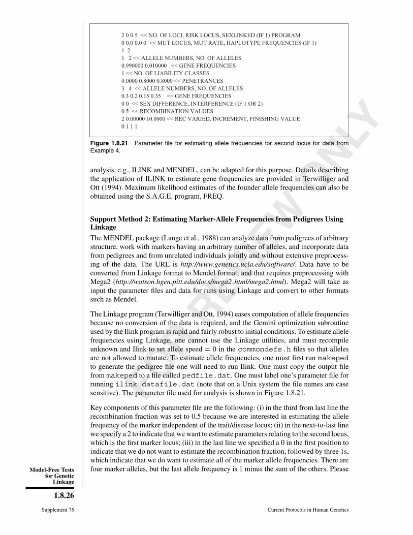
2 0 0 5 << NO. OF LOCI, RISK LOCUS, SEXLINKED (IF 1) PROGRAM0 0.0 0.0 0 << MUT LOCUS, MUT RATE, HAPLOTYPE FREQUENCIES (IF 1)1 21 2 << ALLELE NUMBERS, NO. OF ALLELES0.990000 0.010000 << GENE FREQUENCIES1 << NO. OF LIABILITY CLASSES0.0000 0.8000 0.8000 << PENETRANCES3 4 << ALLELE NUMBERS, NO. OF ALLELES0.3 0.2 0.15 0.35 << GENE FREQUENCIES0 0 << SEX DIFFERENCE, INTERFERENCE (IF 1 OR 2)0.5 << RECOMBINATION VALUES2 0.00000 10.0000 << REC VARIED, INCREMENT, FINISHING VALUE0 1 1 1

Figure 1.8.21 Parameter file for estimating allele frequencies for second locus for data fromExample 4.

analysis, e.g., ILINK and MENDEL, can be adapted for this purpose. Details describingthe application of ILINK to estimate gene frequencies are provided in Terwilliger andOtt (1994). Maximum likelihood estimates of the founder allele frequencies can also beobtained using the S.A.G.E. program, FREQ.

Support Method 2: Estimating Marker-Allele Frequencies from Pedigrees UsingLinkage

The MENDEL package (Lange et al., 1988) can analyze data from pedigrees of arbitrarystructure, work with markers having an arbitrary number of alleles, and incorporate datafrom pedigrees and from unrelated individuals jointly and without extensive preprocess-ing of the data. The URL is http://www.genetics.ucla.edu/software/. Data have to beconverted from Linkage format to Mendel format, and that requires preprocessing withMega2 (http://watson.hgen.pitt.edu/docs/mega2 html/mega2.html). Mega2 will take asinput the parameter files and data for runs using Linkage and convert to other formatssuch as Mendel.

The Linkage program (Terwilliger and Ott, 1994) eases computation of allele frequenciesbecause no conversion of the data is required, and the Gemini optimization subroutineused by the Ilink program is rapid and fairly robust to initial conditions. To estimate allelefrequencies using Linkage, one cannot use the Linkage utilities, and must recompileunknown and Ilink to set allele speed = 0 in the commondefs.h files so that allelesare not allowed to mutate. To estimate allele frequencies, one must first run makepedto generate the pedigree file one will need to run Ilink. One must copy the output filefrom makeped to a file called pedfile.dat. One must label one’s parameter file forrunning ilink datafile.dat (note that on a Unix system the file names are casesensitive). The parameter file used for analysis is shown in Figure 1.8.21.

Key components of this parameter file are the following: (i) in the third from last line therecombination fraction was set to 0.5 because we are interested in estimating the allelefrequency of the marker independent of the trait/disease locus; (ii) in the next-to-last linewe specify a 2 to indicate that we want to estimate parameters relating to the second locus,which is the first marker locus; (iii) in the last line we specified a 0 in the first position toindicate that we do not want to estimate the recombination fraction, followed by three 1s,which indicate that we do want to estimate all of the marker allele frequencies. There arefour marker alleles, but the last allele frequency is 1 minus the sum of the others. Please

FOR

REVIEW

ONLY

GeneticMapping

1.8.27


note that the number of alleles described by the marker locus must equal the number inthe datafile, otherwise Ilink will start but will not reach a convergent solution.

Interpretation of results

The allele-frequency estimates for marker M2 in Figure 1.8.3 obtained by a Linkageanalysis were 0.299087 0.252928 0.275219 0.172766, respectively, for thefour alleles. These figures are shown in the last step of the iteration results when theprogram is run. It is evident that these estimates depart rather markedly from the valuesthat were given (0.3, 0.3, 0.05, and 0.35; see Table 1.8.4). In particular, the “3” allele ismore common than expected. Analysis of allele frequencies from a single family wouldnot be expected to yield reliable estimates. However, if analyses of several familiesshowed a large discrepancy between the assumed frequency of the marker allele that wasobtained from the literature or from considering a reference set of individuals, one mightconsider using the allele frequencies estimated from the data.

COMMENTARY

Choice of MethodsThe choice of methods for genetic linkage

analysis is highly variable and depends uponthe data that are available. For complex dis-eases and traits that result from the interplayof genetic and environmental factors, the ini-tial application of parametric methods can beproblematic because of difficulties in provid-ing an approximately correct genetic model.Model-free methods provide a rapid approachfor assessing evidence of genetic linkage. Innuclear families, model-free methods that onlyuse affected relatives are equivalent to cer-tain parametric models (see below). Therefore,analyses under “model-free” versus model-based approaches should not be viewed as in-dependent or mutually exclusive. Model-freemethods are inefficient in jointly estimatingthe recombination fraction with the genetic ef-fects. Therefore, the recombination fraction istypically assumed to be zero, and the model-free tests for genetic linkage identify regionsshowing evidence for linkage. Parametric ap-proaches will often then be applied to assistin developing a genetic model and to local-ize the underlying major gene. In particular,the mod score approach (Hodge and Elston,1994) described below, in which the lod scoreis maximized over the recombination fractionand the parameters describing the expressionof the phenotype, has been shown to give unbi-ased estimates of all parameters; this methodmoreover does not require knowledge of theascertainment scheme.

The choice of model-free methods dependsupon the type of data that have been gathered.GENEHUNTER PLUS is an efficient tool for

preliminary genomic screening of data be-cause it can process markers from entire chro-mosomes jointly. However, when extendedpedigrees must be divided prior to analyseswith concomitant loss of power, additionalfollow-up studies should be implemented forany region that shows suggestive evidence forlinkage by GENEHUNTER PLUS analysis(i.e., lod scores greater than perhaps 1.0 orNPL scores larger than 2). For qualitative data,a parametric approach can be used with thepenetrance set near zero, so that only affectedindividuals are retained for analysis. This ap-proach can accommodate pedigrees that con-tain multiple generations of affected individu-als in analyses where less polymorphic loci areavailable. For this type of analysis, a geneticmodel (dominant or recessive) is assumed, sothat multiple runs must be performed and acorrection for multiple tests is required. Fi-nally, for quantitative data where the pedigreesare randomly selected, either the likelihood orHaseman-Elston components-of-variance ap-proache provides excellent power as comparedwith parametric approaches.

Alternative Approaches: Using lodScore Approaches to ApproximateModel-Free Analysis

Lod score methods can be applied in a num-ber of ways to obtain approximately model-free tests for genetic linkage. The simplestapproach is to set the penetrance of the dis-ease genotypes close to 0, and the sporadicrisk (i.e., the risk among disease-gene noncar-riers) much closer to 0. For example, the pen-etrance and sporadic risk (given, e.g., by line 7

FOR

REVIEW

ONLY


Linkage

1.8.28


of Fig. 1.8.6) may be divided by 100 to approx-imate a model-free analysis. This modelingscheme essentially includes only results fromanalysis of the affected individuals. Based onlyon their phenotype, unaffected individuals arealmost equally likely to be either carriers ornoncarriers; they are therefore uninformativefor the linkage analysis.

This approach is not strictly model-free be-cause one still must assume a genetic model(i.e., dominant or recessive). Nevertheless, theapproach has been shown in simulation stud-ies to provide a good preliminary test for link-age (Risch et al., 1989). Moreover, unlike allof the model-free methods discussed in thisunit, the method uses all of the marker datain the analysis; it may therefore be the bestchoice for some studies. In particular, use of alod score approach assuming low penetranceis a reasonable first step in analysis when thesporadic risk can be assumed to be much lessthan the carrier risk, when either a dominantor recessive model seems plausible to explainpart of the disease pattern in families, whenthe data are not clustered in nuclear families,and when markers for analysis are not highlypolymorphic.

A second approach for applying lod scoremethods for complex diseases is the mod scoreapproach (Hodge and Elston, 1994), in whichthe lod score is maximized over both the pen-etrance and the recombination fraction. Thismethod has been shown both theoretically andin simulation studies to provide unbiased esti-mates of both the recombination fraction andthe penetrance. However, because the pene-trance parameters are estimated jointly withthe recombination fraction, the power to detectgenetic linkage is reduced in this type of anal-ysis. Another difficulty with the mod score ap-proach is the current lack of well-documentedcomputer programs for this type of analysis.

A maximum-likelihood-binomial analysisprocedure has been developed by Abel andMuller-Myhsok (1998), and these inves-tigators created programs called MLBGH(ftp://ftp.biomath.jussieu.fr/pub/mlbgh). Thismethod compares a likelihood that includesa binomial parameter reflecting increasedIBD sharing to a likelihood with randomsharing. In concept, the method is similarto earlier work by Risch (1990a,b), whichforms the bases for the MLS statistic, a partof the MAPMAKER/SIBS program (ftp://ftp-genome.wi.mit.edu/distribution/software/sibs).The MLBGH procedure had slightly improvedpower over the usual MLS test.

Power ConsiderationsIn nuclear families, the ASP mean-test

approach is identical to genetic analysis undera rare recessive model with no sporadic cases(Knapp et al., 1994). For extended families,the correspondence between parametric andmodel-free methods is not clear. Whittemore(1996) provided a comparison in nuclearfamilies of the weight functions employed byseveral different model-free tests for linkage,along with the corresponding parametricforms that these procedures actually fit. TheSIBPAIR test available from Joe Terwilliger,622 West 168th Street PH 18-302 New YorkN.Y. 10032, uses a recessive parametric modelto obtain a “model-free” test for linkage.SIBPAIR is a part of the ANALYZE package(ftp://ftp.ebi.ac.uk/pub/software/linkage andmapping/linkage cpmc columbia/analyze/).This package performs a variety of usefultests including parametric linkage analysis,transmission disequilibrium tests, and affectedsib-pair tests.

Davis and Weeks (1997) compared 23 dif-ferent model-free tests for linkage applied tosimulated data generated under several dif-ferent two-locus models for disease etiology.The data were simulated to represent modelsthat might reflect the underlying causation forunipolar and bipolar disorders and reflecteda high disease prevalence (7%) and moderaterecurrence risks to first-degree relatives (25%to 30%). For nuclear families, many of thetests had similar power. The SIBPAL tests gen-erally performed quite well relative to othertests. Tests with relatively low power in nu-clear families included the Affected PedigreeMember (Weeks and Lange, 1988) and theGENEHUNTER tests. The GENEHUNTERtest had poor power because the variance ofthe test statistic is constructed assuming that acompletely informative marker locus is avail-able for both parents. GENEHUNTER PLUSrelaxes this assumption, so that the power ofGENEHUNTER PLUS tests should be com-parable to other tests such as SIBPAL. Theaffected pedigree member method is not cov-ered in this chapter because it is very sensitiveto the allele frequencies that are specified.

Another consideration in deciding whichmethod is the most powerful is the type ofdata available. When most of the data areclustered in nuclear families, ASP proceduresare easily conducted and powerful. On theother hand, if the data consist of extendedfamilies with affected individuals scatteredacross each family, then ASP methods will

FOR

REVIEW

ONLY

GeneticMapping

1.8.29


have little power, and methods for pedigreessuch as GENEHUNTER PLUS, Merlin, orRELPAL (Olson and Wijsman, 1993) mustbe used. In theory, whenever appropriate dataare available, multipoint analyses should beconducted. An adaptation of the LINKAGEprogram (Curtis and Sham, 1994) providesan approach that will allow complete use ofall marker data in constructing IBD sharingfor arbitrarily related individuals, but thismethod is computationally slow. Fulker andCardon (1994) developed an approximationthat can be rapidly used to estimate IBDsharing from multiple linked genetic markersin nuclear families. This algorithm hasbeen extended for use in large pedigrees byAlmasy and Blangero (1998) and imple-mented in their package, SOLAR (http://www.sfbr.org/sfbr/public/software/solar/index.html).SOLAR can also take as its input the estimatedidentity by descent sharing from Monte CarloMarkov-Chain implementations such asMorgan (Wijsman et al., 2006). This programdevelops approximations of the likelihood formultipoint analysis of large pedigrees. TheS.A.G.E. program GENIBD also computesmultipoint allele sharing statistics for all pairsin an extended pedigree, provided there areno consanguineous matings.

Tests for Quantitative DataThis unit does not discuss in detail methods

for quantitative data. However, a number ofprograms are available. The simplest to applyis the Haseman-Elston approach, which isprovided as part of the SIBPAL package (seeExample 2). Variance components proceduresthat partition interindividual variability intosources linked and unlinked to geneticmarkers have been found to be more powerfulthan other methods (Wijsman and Amos,1997). Therefore, many newer softwarepackages also include a likelihood-based vari-ance components method. GENEHUNTERincludes a variance components procedurefor quantitative traits (http://waldo.wi.mit.edu/ftp/distribution/software/GENEHUNTER/gh2/). The program Analysis of ComplexTraits (ACT) performs variance componentsanalysis under oligogenic and multivariatemodels with allowance for ascertainment. Thepackage is available at http://www.epigenetic.org/linkage/act.html. The package SequentialOligogenic Linkage Analysis Routines (SO-LAR; Almasy and Blangero, 1998) providesa range of tools for analysis of quantitativedata, including marker-allele frequency esti-

mation, procedures to fit oligogenic variancecomponent models under a variety of additiveand epistatic interaction models, and teststhat allow for linkage disequilibrium. Thissoftware is available from http://www.sfbr.org/sfbr/public/software/solar/index.html.Merlin also implements a quantitative test forlinkage.

SOLAR, ACT, GENEHUNTER, and Mer-lin are somewhat similar in their capabilitiesbut have been optimized for different purposes.SOLAR can analyze extremely large familiesand can evaluate very complex genetic mod-els. GENEHUNTER can only analyze smallfamilies, and under rather simple genetic mod-els. ACT includes complex genetic models aswell as ascertainment corrections and the cal-culation of robust test statistics (Amos, 1994;Amos et al., 1996), but applying it to largepedigrees can be slow, as it requires prepro-cessing by either ERPA or GENEHUNTER toobtain IBD sharing. Merlin, ACT, and SOLARall have extensions to handle multivariate data(de Andrade et al., 2002; Bauman et al., 2005;Liang et al., 2009). ACT is more flexible inthe types of multivariate structures it can han-dle, but Merlin is easier to implement. If onewould like to evaluate many traits jointly, themultivariate extension (Amos et al., 1990b) ofthe H-E method is easier to implement andrequires estimation of fewer parameters, andhence is a better screening tool than the vari-ance components methods. There is now atwo-level multivariate extension of the H-Emethod (Wang and Elston, 2007) with a corre-sponding extension in RELPAL to allow morerelative pairs to be jointly analyzed, availablefor computation in S.A.G.E.

Some power comparisons are available forchoosing among test procedures for quanti-tative data. Wijsman and Amos (1997) re-viewed a large number of simulation studiesthat compared power of many different quan-titative tests for linkage applied to either ex-tended families or nuclear families. Demenaisand Amos (1989) found that the Haseman-Elston procedure provided 70% to 90% ofthe power of the parametric linkage approach.Goldgar and Oniki (1992) found that the powerof the correctly specified parametric meth-ods and their model-free methods were sim-ilar when the model for parametric analysiswas estimated from available data. Goldgarand Oniki (1992) and Amos (1994) showedthe power of the Haseman-Elston approachto be ∼80% of that provided by likelihood-based components of variance procedures, but

FOR

REVIEW

ONLY


Linkage

1.8.30


the newer H-E approach (Elston et al., 2000;Shete et al., 2003) can have power similar toother variance components procedures. Oneadvantage of the Haseman-Elston regressionapproach is a correction for possible outliersin the data if they result in a negative inter-cept (S.A.G.E., 2011); another is its compu-tational ease relative to all other methods ofanalysis. Fast H-E methods with extensionsfor multiple markers (Fulker et al., 1995), aswell as similar extensions for likelihood-basedvariance component approaches, clearly pro-vide improved power over single-locus meth-ods; furthermore, studies with multiple mark-ers can provide a localization of the underly-ing genetic locus through an interval mappingstrategy. In this approach, the chromosomal lo-cation yielding the strongest effect of the trait-affecting major gene provides the best estimatefor the location of the trait locus (Lander andBotstein, 1989; Olson, 1995).

For traits having low heritability, the powerof linkage studies can be greatly improvedby selecting families for study based on indi-viduals with extreme phenotypes (Carey andWilliamson, 1991; Cardon and Fulker, 1994;Risch and Zhang, 1995). Analysis of this typeof data has involved regression of the traitvalue of the unselected sib on IBD for the pair.The MLBGH procedure can be used for thistype of data. The variance components soft-ware ACT can analyze data in which familiesare selected based upon the phenotypes of 1 or2 subjects (de Andrade and Amos, 2000). Al-ternatively, the IBD status can be treated as theoutcome and the trait values as the predictors.This approach removes the need to correct forascertainment, since one is conditioning on thetrait values (Sham et al., 2002) and has com-parable power to the components of variancemethods.

Literature CitedAbecasis, G.R., Cherny, S.S., Cookson, W.O., and

Cardon, L.R. 2002. Merlin-rapid analysis ofdense genetic maps using sparse gene flow trees.Nat. Genet. 30:97-101.

Abel, L. and Muller-Myhsok, B. 1998. Robustnessand power of the maximum-likelihood-binomialand maximum-likelihood-score methods, inmultipoint linkage analysis of affected-sibship data. Am. J. Hum. Genet. 63:638-647.

Allison, D.B. and Beasley, M. 1998. A method andcomputer program for controlling the family-wise alpha rate in gene association studies in-volving multiple phenotypes. Genet. Epidemiol.15:87-101.

Almasy, L. and Blangero, J. 1998. Multipointquantitative-trait linkage analysis in generalpedigrees. Am. J. Hum. Genet. 62:1198-1211.

Amos, C.I. 1994. Robust detection of genetic link-age by variance components analysis. Am. J.Hum. Genet. 54:535-543.

Amos, C.I. and Elston, R.C. 1989. Robust methodsfor the detection of genetic linkage for quan-titative data from pedigrees. Genet. Epidemiol.6:349-361.

Amos, C.I., Dawson, D.V., and Elston, R.C. 1990a.The probabilistic determination of identity-by-descent sharing for pairs of relatives from pedi-grees. Am. J. Hum. Genet. 47:842-853.

Amos, C.I., Elston, R.C., Bonney, G.E., Keats,B.J., and Berenson, G.S. 1990b. A multivariatemethod for detecting genetic linkage, with appli-cation to a pedigree with an adverse lipoproteinphenotype. Am. J. Hum. Genet. 47:247-254.

Amos, C.I., Zhu, D., and Boerwinkle, E. 1996. As-sessing genetic linkage and association with ro-bust components of variance approaches. Ann.Hum. Genet. 60:143-166.

Bauman, L.E., Almasy, L., Blangero, J., Duggirala,R., Sinsheimer, J.S., and Lange, K. 2005. Fish-ing for pleiotropic QTLs in a polygenic sea. Ann.Hum. Genet. 69:590-611.

Blackwelder, W.C. and Elston, R.C. 1982. Powerand robustness of sib-pair linkage tests and ex-tension to larger sibships. Commun. Stat. Theor.Methods 11:449-484.

Blackwelder, W.C. and Elston, R.C. 1985. A com-parison of sib pair linkage tests for disease sus-ceptibility loci. Genet. Epidemiol. 2:5-97.

Boehnke, M. 1991. Estimating allele frequencies.Am. J. Hum. Genet. 48:22-25.

Boyles, A.L., Scott, W.K., Martin, E.R., Schmidt,S., Li, Y.J., Ashley-Koch, A., Bass, M.P.,Schmidt, M., Pericak-Vance, M.A., Speer, M.C.,and Hauser, E.R. 2005. Linkage disequilibriuminflates type I error rates in multipoint linkageanalysis when parental genotypes are missing.Hum. Hered. 59:220-227.

Cardon, L.R. and Fulker, D.W. 1994. The power ofinterval mapping of quantitative trait loci, usingselected sib pairs. Am. J. Hum. Genet. 55:825-833.

Carey, G. and Williamson, J.A. 1991. Linkage anal-ysis of quantitative traits: Increased power byusing selected samples. Am. J. Hum. Genet.49:786-796.

Chotai, J. 1984. On the lod score method in linkageanalysis. Ann. Hum. Genet. 48:359-378.

Cox, N.J. and Spielman, R.S. 1989. The insulingene and susceptibility to IDDM. Genet. Epi-demiol. 6:65-69.

Cubells, J.F., Sun, X., Li, W., Bonsall, R.W., Mc-Grath, J.A., Avramopoulos, D., Lasseter, V.K.,Wolyniec, P.S., Tang, Y.L., Mercer, K., Pulver,A.E., and Elston, R.C. 2011. Linkage analysisof plasma dopamine beta-hydroxylase activityin families of patients with schizophrenia. Hum.Genet. 130:635-645.

FOR

REVIEW

ONLY

GeneticMapping

1.8.31


Curtis, D. and Sham, P.C. 1994. Using risk cal-culation to implement an extended relative pairanalysis. Ann. Hum. Genet. 58:151-162.

Davis, S. and Weeks, D.E. 1997. Comparison ofnonparametric statistics for detection of linkagein nuclear families: Single-marker evaluation.Am. J. Hum. Genet. 61:1431-1444.

Davis, S., Schroeder, M., Goldin, L.R., and Weeks,D.E. 1996. Nonparametric simulation-basedstatistics for detecting linkage in general pedi-grees. Am. J. Hum. Genet. 58:867-880.

Dawson, D.V., Kaplan, E.B., and Elston, R.C. 1990.Extensions to sib-pair linkage tests applicableto disorders characterized by late onset. Genet.Epidemiol. 7:153-166.

de Andrade, M. and Amos, C.I. 2000. Ascertain-ment issues in variance components models.Genet. Epidemiol. 19:333-344.

de Andrade, M., Gueguen, R., Visvikis, S., Sass,C., Siest, G., and Amos, C.I. 2002. Extensionof variance components approach to incorporatetemporal trends and longitudinal pedigree dataanalysis. Genet. Epidemiol. 22:221-232.

Demenais, F.M. and Amos, C.I. 1989. Power ofthe sib-pair and lodscore methods for linkageanalysis of quantitative traits. Prog. Clin. Biol.Res. 329:201-206.

Elston, R.C., Buxbaum, S., Jacobs, K.B., and Olson,J.M. 2000. Haseman and Elston revisited. Genet.Epidemiol. 19:1-17.

Feingold, E., Brown, P.O., and Siegmund, D. 1993.Gaussian models for genetic linkage analysisusing complete high-resolution maps of identityby descent. Am. J. Hum. Genet. 53:234-251.

Fulker, D.W. and Cardon, L.R. 1994. A sib-pairapproach to interval mapping of quantitative traitloci. Am. J. Hum. Genet. 54:1092-1103.

Fulker, D.W., Cherny, S.S., and Cardon, L.R.1995. Multipoint interval mapping of quantita-tive trait loci, using sib pairs. Am. J. Hum. Genet.56:1224-1233.

Goldgar, D.E. and Oniki, R.O. 1992. Compari-son of a multipoint identity by descent methodwith parametric multipoint linkage analysis formapping quantitative traits. Am. J. Hum. Genet.50:598-606.

Haseman, J.K. and Elston, R.C. 1972. The inves-tigation of linkage between a quantitative traitand a marker locus. Behav. Genet. 2:3-19.

Huang, Q., Shete, S., and Amos, C.I. 2004. Ignor-ing linkage disequilibrium among tightly linkedmarkers induces false-positive evidence of link-age for affected sib pair analysis. Am. J. Hum.Genet. 75:1106-1112.

Hodge, S.E. 1984. The information contained inmultiple sibling pairs. Genet. Epidemiol. 1:109-122.

Hodge, S.E. and Elston, R.C. 1994. Lods, wrods,and mods: The interpretation of lod scores calcu-lated under different models. Genet. Epidemiol.11:329-342.

Igo, R.H. Jr. and Schnell, A.H. 2012. Comparisonof requirements and capabilities of major multi-

purpose software packages. Methods Mol. Biol.850:539-558.

Knapp, M., Seuchter, S.A., and Baur, M.P. 1994.Linkage analysis in nuclear families. II. Rela-tionship between ASP and lod score tests. Hum.Hered. 44:44-51.

Kong, A. and Cox, N.J. 1997. Allele-sharing mod-els: LOD scores and accurate linkage tests. Am.J. Hum. Genet. 61:1179-1188.

Kruglyak, L. and Lander, E.S. 1995. Complete mul-tipoint sib-pair analysis of qualitative and quan-titative traits. Am. J. Hum. Genet. 57:439-454.

Kruglyak, L., Daly, M.J., and Lander, E.S. 1995.Rapid multipoint linkage analysis of recessivetraits in nuclear families including homozygos-ity mapping. Am. J. Hum. Genet. 56:519-527.

Kruglyak, L., Daly, M.J., Reeve-Daly, M.P., andLander, E.S. 1996. Parametric and nonparamet-ric linkage analysis: A unified multipoint ap-proach. Am. J. Hum. Genet. 58:1347-1363.

Lander, E.S. and Botstein, D. 1989. MappingMendelian factors underlying quantitative traitsusing RFLP linkage maps. Genetics 121:185-199.

Lander, E.S. and Kruglyak, L. 1995. Genetic dis-section of complex traits: Guidelines for inter-preting and reporting linkage results. Nat. Genet.11:241-247.

Lange, K., Weeks, D., and Boehnke, M. 1988.Programs for pedigree analysis: MENDEL,FISHER, and dGENE. Genet. Epidemiol. 5:471-472.

Liang, L., Chen, W.M., Sham, P.C., and Abecasis,G.R. 2009. Variance components linkage anal-ysis with repeated measurements. Hum. Hered.67:237-247.

Morton, N.E. 1998. Significance levels in complexinheritance. Am. J. Hum. Genet. 62:690-697.

Olson, J.M. 1995. Robust multipoint linkage anal-ysis: An extension of the Haseman-Elstonmethod. Genet. Epidemiol. 12:163-176.

Olson, J.M. and Wijsman, E. 1993. Linkage be-tween quantitative trait and marker locus: Meth-ods using relative pairs. Genet. Epidemiol.10:87-102.

Ott, J. 1992. Strategies for characterizing highlypolymorphic markers in human gene mapping.Am. J. Hum. Genet. 51:283-290.

Ott, J. 1999. Analysis of Human Genetic Linkage,3rd ed. Johns Hopkins University Press, Balti-more, Maryland.

Palmer, L.J., Jacobs, K.B., and Elston, R.C. 2000.Haseman and Elston revisited: The effects ofascertainment and residual familial correlationson power to detect linkage. Genet. Epidemiol.19:456-460.

Risch, N. 1990a. Linkage strategies for geneticallycomplex traits. I. Multilocus models. Am. J.Hum. Genet. 16:222-228.

Risch, N. 1990b. Linkage strategies for geneticallycomplex traits. III. The effect of marker poly-morphism on analysis of affected relative pairs.Am. J. Hum. Genet. 16:242-253.

FOR

REVIEW

ONLY


Linkage

1.8.32


Risch, N. and Zhang, H. 1995. Extreme discordantsib pairs for mapping quantitative trait loci inhumans. Science 268:1584-1589.

Risch, N., Claus, E., and Giuffra, L. 1989. Linkageand mode of inheritance in complex traits. Prog.Clin. Biol. Res. 329:183-188.

Rosner, B. 1982. Fundamentals of Biostatistics pp.317-323. Duxbury Press, Boston.

Sawcer, S., Jones, H.B., Judge, D., Visser, F.,Compston, A., Goodfellow, P.N., and Clayton,D. 1997. Empirical genomewide significancelevels established by whole genome simulators.Genet. Epidemiol. 14:223-229.

Schnell, A.H., Sun, X., Igo, R.H. Jr., and Elston,R.C. 2011. Some capabilities for model-basedand model-free linkage analysis using the pro-gram package. S.A.G.E. (statistical analysis forgenetic epidemiology). Hum. Hered. 72:237-246.

Schaid, D.J. and Nick, T.G. 1990. Sib-pair link-age tests for disease susceptibility loci: Com-mon tests vs. the asymptotically most powerfultests. Genet. Epidemiol. 7:359-370.

Sham, P.C., Purcell, S., Cherny, S.S., and Abeca-sis, G.R. 2002. Powerful regression-basedquantitative-trait linkage analysis of generalpedigrees. Am. J. Hum. Genet. 71:238-253.

Shete, S., Jacobs, K.B., and Elston, R.C. 2003.Adding further power to the Haseman and Elstonmethod for detecting linkage in larger sibships:Weighting sums and differences. Hum. Hered.55:79-85.

Sinha, R. and Gray-McGuire, C. 2008. Haseman-Elston regression in ascertained samples: Impor-tance of dependent variable and mean correctionfactor selection. Hum. Hered. 65:66-76.

Statistical Analysis for Genetic Epidemiology(S.A.G.E.). 2011. Case Western Reserve Uni-versity, Cleveland, Ohio.

Stewart, W.C., Drill, E.N., and Greenberg, D.A.2011. Finding disease genes: A fast and flexibleapproach for analyzing high-throughput data.Eur. J. Hum. Genet. 19:1090-1094.

Suarez, B.K. and Van Eerdewegh, P. 1984. A com-parison of three affected-sib-pair scoring meth-ods to detect HLA-linked disease susceptibilitygenes. Am. J. Med. Genet. 18:135-146.

Suarez, B.K., Rice, J., and Reich, T. 1978. The gen-eralized sib pair IBD distribution: Its use in thedetection of linkage. Ann. Hum. Genet. Lond.42:87-94.

Terwilliger, J.D. and Ott, J. 1994. Handbook of Hu-man Genetic Linkage. Johns Hopkins UniversityPress, Baltimore, Maryland.

Thornton, T.A. and Haines, J.L. 2003. PowerTrim:An automated decision support algorithm forpreprocessing family-based genetic data. Am. J.Hum. Genet. 72:1280-1281.

Wang, T. and Elston, R.C. 2005. Two-levelHaseman-Elston regression for general pedigreedata analysis. Genet. Epidemiol. 29:12-22.

Wang, T. and Elston, R.C. 2007. Regression-basedmultivariate linkage analysis with an applicationto blood pressure and body mass index. Ann.Hum. Genet. 71:96-106.

Weeks, D.E. and Lange, K. 1988. The affected-pedigree-member method of linkage analysis.Am. J. Hum. Genet. 42:315-326.

Weeks, D.E., Lehner, T., Squires-Wheeler, E.,Kaufman, C., and Ott, J. 1990. Measuring theinflation of the lod score due to its maximiza-tion over model parameters in human linkageanalysis. Genet. Epidemiol. 7:237-243.

Whittemore, A.S. 1996. Genome scanning for link-age: An overview. Am. J. Hum. Genet. 59:704-716.

Wijsman, E.M. and Amos, C.I. 1997. Genetic anal-ysis of simulated oligogenic traits in nuclear andextended pedigrees: Summary of GAW10 con-tributions. Genet. Epidemiol. 14:719-735.

Wijsman, E.M., Rothstein, J.H., and Thompson,E.A. 2006. Multipoint linkage analysis withmany multiallelic or dense diallelic markers:Markov chain-Monte Carlo provides practicalapproaches for genome scans on general pedi-grees. Am. J. Hum. Genet. 79:846-858.

model-free tests for genetic linkage unit 1 · pdf file · 2017-08-27when...

Documents