model for uptake of organic chemicals by plants
TRANSCRIPT
Station Bulletin 677May 1990
Model for Uptakeof Organic Chemicals by Plants
Agricultural Experiment StationOregon State University
THIS P
UBLICATIO
N IS O
UT OF D
ATE.
For mos
t curr
ent in
formati
on:
http:/
/exten
sion.o
regon
state.
edu/c
atalog
MODEL FOR UPTAKE OF ORGANIC CHEMICALS BY PLANTS
L. BOERSMA, F. T. LINDSTROM, C. MCFARLANE
AUTHORS: F. T. Lindstrom and L. Boersma, Department of Soil Science,
Oregon State University; C. McFarlane, Research Scientist, Corvallis
Environmental Research Laboratory, United States Environmental Protec-
tion Agency.
THIS P
UBLICATIO
N IS O
UT OF D
ATE.
For mos
t curr
ent in
formati
on:
http:/
/exten
sion.o
regon
state.
edu/c
atalog

FOREWORD
The uptake, transport, and accumulation of organic and inorganicchemicals by plants are influenced by characteristics of the plant,properties of the chemical, properties of the soil, and by prevailingenvironmental conditions. Complex interrelationships exist between thephysical, chemical, and physiological processes that occur in specificplant tissues and the response of these processes to environmentalconditions, such as the daily cycle of radiation, evaporation, and airtemperature. The uptake is further influenced by the availability ofthe chemical at the root surface, determined in turn by transport char-acteristics of the soil. Also important is the behavior of the chemi-cal in the rhizosphere and the ease with which it moves across limitingmembranes at the root surface.
This report describes the development of a predictive simulatorfor the uptake of xenobiotic chemicals by plants from the soil solu-tion. The model is based on definition of the plant as a set of com-partments separated from each other by thin membranes. Movement ofwater and solutes between compartments occurs by mass flow and diffu-sion. The compartments represent major pools for accumulation of waterand solutes. Anatomical features of the compartments and the manner inwhich they are connected are described by a series of equations basedon conservation of mass. Experimental data were used to calibrate andthen validate the model.
ACKNOWLEDGMENTS
This publication reports results of studies supported, in part, byResearch Grant CR 811940-01-0 "A Mathematical Model of the Bjoaccumula-tion of Xenobiotic Organic Chemicals in Plants" from the CorvallisEnvironmental Research Laboratory of the United States EnvironmentalProtection Agency to the Department of Soil Science at Oregon StateUniversity and by the Oregon Agricultural Experiment Station.
1
THIS P
UBLICATIO
N IS O
UT OF D
ATE.
For mos
t curr
ent in
formati
on:
http:/
/exten
sion.o
regon
state.
edu/c
atalog

CONTENTS
Page
FOREWORD 1
ACKNOWLEDGEMENTS
FIGURES iv
TABLES V111
SUMMARY 1
DEVELOPMENT OF THE MODELIntroduction 3
Structure of the Model 4
Sequence of Compartments 7
Mass Balance Equations 13
Soil Compartment 14
Free Space of the Roots 15
Storage Volume of Root Cortex 18
Root Xylem Compartment 19
Root Storage Compartment 21
System of Equations 22
Solution Method 23
Effective Concentrations 26
APPLICATION TO EXPERIMENTS 29
Introduction 29
Experimental Procedures 29
Qualitative Overview of Results 36
Calibration 39
Volumes of Compartments 43
Chemical and Physical Parameters 45
Phloem Transport 46
Concentration of Bromacil in Bathing Solution 47
Transpiration RatesStorage Coefficients 48
DISCUSSION 50
Introduction 50
Roots 61
Stems 64
Leaves 64
THIS P
UBLICATIO
N IS O
UT OF D
ATE.
For mos
t curr
ent in
formati
on:
http:/
/exten
sion.o
regon
state.
edu/c
atalog
CONTENTS (continued)
Page
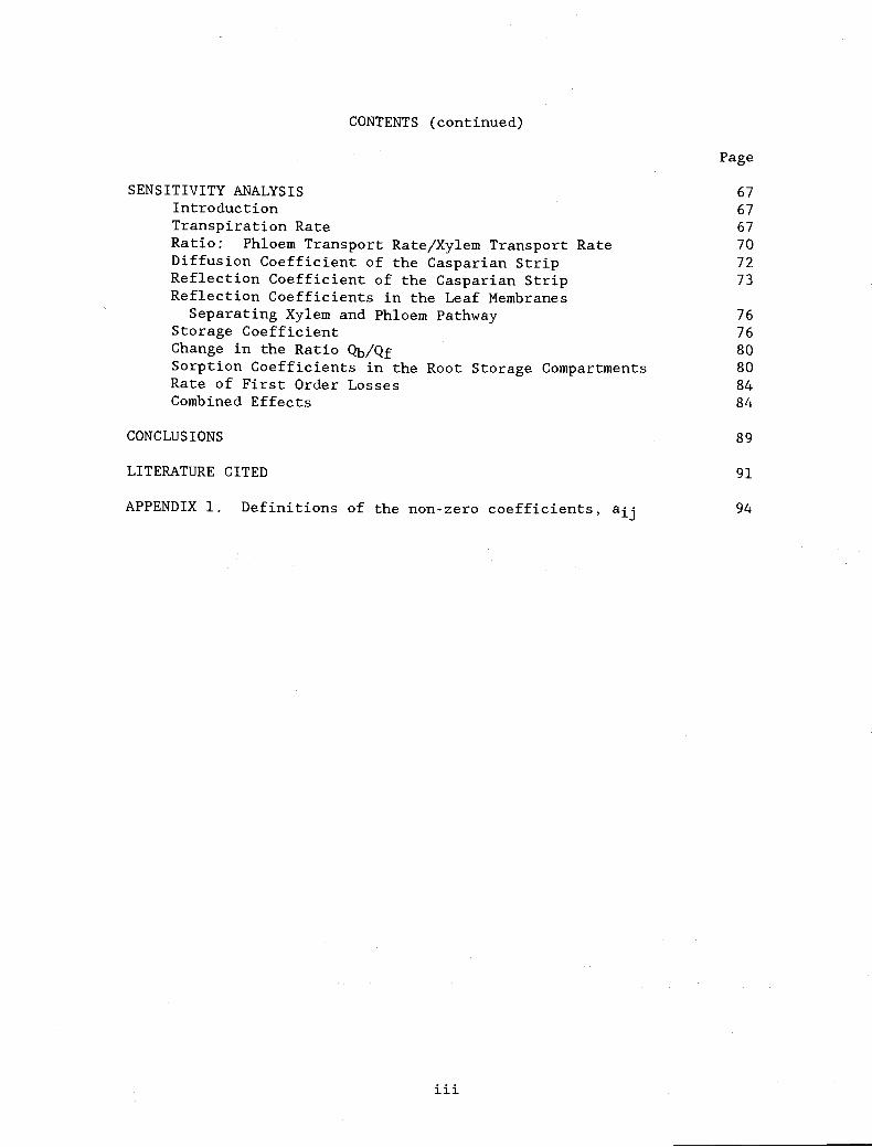
SENSITIVITY ANALYSIS 67Introduction 67Transpiration Rate 67Ratio: Phloem Transport Rate/Xylem Transport Rate 70
Diffusion Coefficient of the Casparian Strip 72
Reflection Coefficient of the Casparian Strip 73
Reflection Coefficients in the Leaf MembranesSeparating Xylem and Phloem Pathway 76
Storage Coefficient 76Change in the Ratio Qb/Qf 80
Sorption Coefficients in the Root Storage Compartments 80Rate of First Order Losses 84Combined Effects 84
CONCLUSIONS 89
LITERATURE CITED 91
APPENDIX 1. Definitions of the non-zero coefficients, ajj 94
111
THIS P
UBLICATIO
N IS O
UT OF D
ATE.
For mos
t curr
ent in
formati
on:
http:/
/exten
sion.o
regon
state.
edu/c
atalog
iv
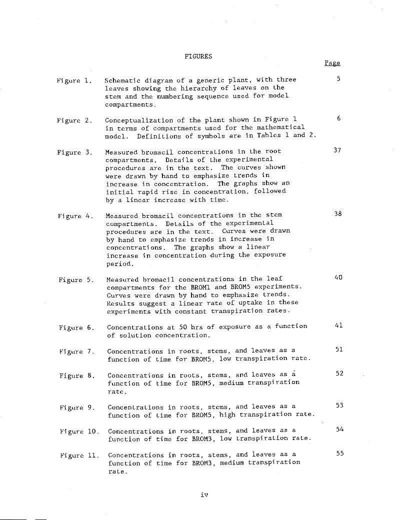
FIGURESPage
Figure 1. Schematic diagram of a generic plant, with three 5
leaves showing the hierarchy of leaves on thestem and the numbering sequence used for modelcompartments.
Figure 2. Conceptualization of the plant shown in Figure 1 6
in terms of compartments used for the mathematicalmodel. Definitions of symbols are in Tables 1 and 2.
Figure 3. Measured bromacil concentrations in the root 37
compartments. Details of the experimentalprocedures are in the text. The curves shown
were drawn by hand to emphasize trends inincrease in concentration. The graphs show aninitial rapid rise in concentration, followedby a linear increase with time.
Figure 4. Measured bromacil concentrations in the stem 38
compartments. Details of the experimentalprocedures are in the text. Curves were drawnby hand to emphasize trends in increase inconcentrations. The graphs show a linearincrease in concentration during the exposureperiod.
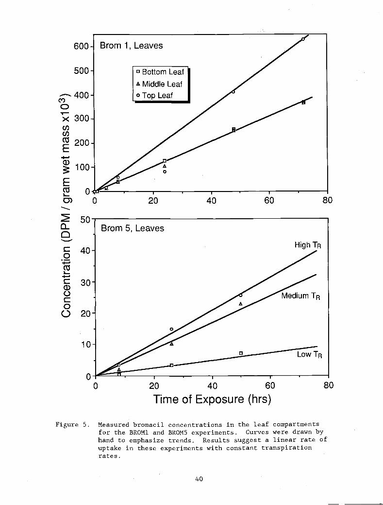
Figure 5. Measured bromacil concentrations in the leaf 40
compartments for the BROM1 and BROM5 experiments.Curves were drawn by hand to emphasize trends.Results suggest a linear rate of uptake in theseexperiments with constant transpiration rates.
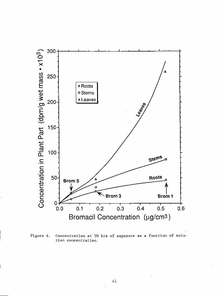
Figure 6. Concentrations at 50 hrs of exposure as a function 41
of solution concentration.
Figure 7. Concentrations in roots, stems, and leaves as a 51
function of time for BROM5, low transpiration rate.
Figure 8. Concentrations in roots, stems, and leaves as 52
function of time for BROM5, medium transpirationrate.
Figure 9. Concentrations in roots, stems, and leaves as a 53
function of time for BROM5, high transpiration rate.
Figure 10. Concentrations in roots, stems, and leaves as a 54
function of time for BROM3, low transpiration rate.
Figure 11. Concentrations in roots, stems, and leaves as a 55
function of time for BROM3, medium transpirationrate.
THIS P
UBLICATIO
N IS O
UT OF D
ATE.
For mos
t curr
ent in
formati
on:
http:/
/exten
sion.o
regon
state.
edu/c
atalog

FIGURES (continued)Page
Figure 12. Concentrations in roots, stems, and leaves as a 56
function of time for BROM3, high transpirationrate.
Figure 13. Concentrations in roots, stems, and leaves as a 57
function of time for BRON1.
Figure 14. Ratio Qf/Qb for the root cortex and for root 63
storage compartments as a function oftranspiration rate.
Figure 15. Forward storage coefficients for stem compartments 65
plotted as a function of volumes of stem storagecompartments.
Forward storage coefficients for leaf compartmentsplotted as a function of volumes of leaf storagecompartments.
Simulations showing the effect of changing thetranspiration rate. Reference simulation waswith BROM5, medium transpiration rate,Tr = 5.67 cm3/hr. Comparisons are with lowtranspiration rate Tr = 2.00 cm3/hr (curves A)and high transpiration rate, Tr = 7.80 cm3/hr(curves B).
Simulations showing the effects of changing theratios of phloem transport rate divided by xylemtransport rate. Reference simulation was withthe fractions set to f1 = 0.3; f2 = 0.2, f3 = 0.1.Simulation A: f1 = 0.0; f2 = 0.0, f3 = 0.0, andSimulation B: f1 = 0.15; f2 = 0.15, and f3 = 0.1.
Simulations showing the effects of changing thediffusion coefficient of the boundary representingthe Casparian strip. Reference simulation was with
D = 1.8 x 0.l0 cm2/hr. Simulation A: D = 1.8 x10⁻⁶ cm2/hr, simulation B: D = 1.8 x 10⁻⁸ cm2/hr.
Simulation showing effects of changing the reflec-tion coefficient of the boundary representng theCasparian strip. Reference simulation was with
a = 0.0. Simulation A: a = 0.2; simulation B:a = 0.7.
V
66
69
71
74
75
Figure 16.
Figure 17.
Figure 18.
Figure 19.
Figure 20.THIS
PUBLIC
ATION IS
OUT O
F DATE.
For mos
t curr
ent in
formati
on:
http:/
/exten
sion.o
regon
state.
edu/c
atalog

vi
FIGURES (continued)Page
Figure 21. Simulations showing the effects of changing the 77
reflection coefficients of the membranes in theleaves which separate phloem from xylem (aiO,al4, and a18). Reference simulation was withthe three coefficients equal to zero. Simula-
tion A, a's equal to 0.2; Simulation B, a'sequal to 0.7.
Figure 22. Simulations showing the effect of increasing or 79
decreasing values of the forward (Qb) andbackward (Qb) coefficients while maintainingthe same ratio Qf/Qb. The reference simulationwas with all Qf's and Qb's as in Table 8. For
Simulation A, all coefficients were divided bytwo; for Simulation B, all storage coefficientswere multiplied by two.
Figure 23. Simulations showing the effects of changing the 81
ratios of forward storage coefficients to thebackward storage coefficients. Referencesimulation was with all storage coefficients asshown in Table 8. For Simulation A, all forwardstorage coefficients (Q) were divided by twowhile leaving the Qb the same; for Simulation B,all forward storage coefficients were multipliedby two, while leaving the Qb' the same.
Figure 24. Simulations showing the effects of changing the 82
sorption coefficients (B's) in the rootcompartments. These coefficients immobilizechemical so that the coefficient has an effectthat is similar to that of increasing ordecreasing the volume of the compartment.Reference simulation was with values of thesorption coefficients B = 0. Simulation A,
sorption coefficients of the two rootcompartments, B1 = B3 = 0.5; Simulation B,sorption coefficient of the two root compart-ments, Bi = B3 = 1.0.
Figure 25. Simulations showing effects of changing the rates 83
of first order loss (A) in the leaves. Reference
simulation was with all A's equal to zero.Simulation A: A15 = 0.0016, A18 = 0.00175,A21 = 0.0018; simulation B: A15 = 0.0032,
A18 = 0.0035, A21 = 0.0036; simulation C:A15 = 0.0064, A18 = 0.0070, A21 = 0.0072.
THIS P
UBLICATIO
N IS O
UT OF D
ATE.
For mos
t curr
ent in
formati
on:
http:/
/exten
sion.o
regon
state.
edu/c
atalog
vii
FIGURES (continued)Page
Figure 26. Simulations showing the combined effects of 87
changing several parameters at the same time.Reference simulation was with data set for BROM5,medium transportation rate (Table 8). Valuesof parameters used for this simulation are inTable 13.
Figure 27. Simulation showing the combined effects of 88
changing several parameters. Referencesimulation was with data set for BROM5, mediumtranspiration rate (Table 8). Values ofparameters used for this simulation are inTable 13.
THIS P
UBLICATIO
N IS O
UT OF D
ATE.
For mos
t curr
ent in
formati
on:
http:/
/exten
sion.o
regon
state.
edu/c
atalog
TABLESPage
Table 1. Notation used in the model. 8
Table 2. Definitions of symbols and subscripts used to 9
identify compartments, mass of chemical incompartments and concentrations.
Table 3. Fluid flow rules. Qii Ql5, and Q19 arespecified transpiration rates (cm3/h) where thefractions of total transpiration allocated toeach leaf cluster are f1 to Qll f2 to Ql5 andf3 to Ql9.
viii
10
Table 4. Environmental parameters and plant functions 31
during uptake test (BROM3).
Table 5. Measured transpiration rates, leaf areas, and 33
wet masses of roots, stems, and leaves for threeexperiments with different bromacil concentra-tions. The data shown are averages of severalmeasurements obtained during an experimentalperiod of 220 hrs for BROM5, 55 hrs for BROM3,and 72 hrs for BROM1. Number in parenthesisfollowing leaf area and mass of wet plantmaterial is estimated standard error (ese).
Table 6. Bromacil concentrations in DPM per gram wet biomass. 35
Table 7. Basis for calculating the compartment volumes of 44
the experimental plants. The example shown isBROM5, medium transpiration rate.
Table 8. Values of parameters used in UTAB 4.6 for 46
geometric and chemical properties for eachcompartmental boundary and fluid flow rate.
Table 9. Simulated concentrations (Ce) divided by measured 58
concentrations (Cexp) at three transpiration rates.
Table 10. Values of storage (forward) and mobilization 59
(backward) transfer coefficient determined bythe calibration procedure used in the text.
Table 11. Ratios Qf/Qb for individual plant parts. The 62
transpiration rate for each experiment is listedat the top of each data column in the units ofl0 cm3/cm2 hr.
THIS P
UBLICATIO
N IS O
UT OF D
ATE.
For mos
t curr
ent in
formati
on:
http:/
/exten
sion.o
regon
state.
edu/c
atalog

ix
TABLES (continued)Page
Table 12. Values of parameters used in the sensitivity 68
simulations. The data base for BROM5, mediumtranspiration rate was the reference level forthese simulations.
Table 13. Values of the parameters used for simulations in 86
which several parameters were changed for anevaluation of combined effects.
THIS P
UBLICATIO
N IS O
UT OF D
ATE.
For mos
t curr
ent in
formati
on:
http:/
/exten
sion.o
regon
state.
edu/c
atalog
MATHEMATICAL MODEL OF PLANT UPTAKE OF ORGANIC CHEMICALS
SUMMARY
Uptake, in-plant transport, and local accumulation of organic
chemicals by plants are influenced by plant characteristics, properties
of the chemical and the soil, and by environmental conditions. Evalua-
tions of plant contamination required by regulatory agencies cannot be
made experimentally for the many thousands of xenobiotic chemicals in
existence or being developed. A predictive simulator in the form of a
mathematical model would provide a valuable tool for such evaluations.
For this reason, a mathematical model (UTAB, uptake, Translocation,
Accumulation, Biodegradation) was formulated by defining a generic
plant as a set of adjacent compartments representing the major pools
involved in transport and accumulation of water and solutes. The model
consists of one root compartment, three stem compartments, and three
leaf compartments. Each compartment is subdivided into two transport
compartments, one for xylem and one for phloem, and a storage compart-
ment. In addition, two compartments model the root volume outside the
Casparian strip, one for the apparent free space and one for the cell
volume. Values for the anatomical dimensions of the compartments and
for physical and chemical coefficients were chosen from the literature.
The complete system of equations, which describes uptake and accumula-
tion, consists of 24 differential equations which are solved in terms
of the chemical mass in each compartment as a function of time. The
solution procedure is also developed and presented.
For calibration purposes, concentrations measured in roots, stems,
and leaves were compared with model predictions, while model parameters
were changed until no further improvement in matching model predictions
THIS P
UBLICATIO
N IS O
UT OF D
ATE.
For mos
t curr
ent in
formati
on:
http:/
/exten
sion.o
regon
state.
edu/c
atalog

with experimental results was obtained. This exercise revealed impor-
tant plant behavior that was not accounted for in the original formula-
tion of the model and, as such, showed the value of the model for
elucidating plant response.
The model satisfactorily predicted the observed uptake and distri-
bution patterns for bromacil in soybean plants, at the stage of growth
and under the environmental conditions used in the experiments, involv-
ing a range of transpiration rates. This indicates that the model is
flexible enough to provide an accurate representation of uptake and the
influence of transpiration rate on the uptake and translocation of this
chemical. Parameter values used in the model were selected from
literature and experimental observation. They functioned well in these
simulations and they are appropriately applied in the model. The
chemical parameters for storage, mobilization, and diffusion when used
in the model also yielded satisfactory results, suggesting that they
are also appropriately applied. Finally, the calibration, although of
limited scope, showed that the model equations yielded an accurate
picture of the actual uptake patterns for bromacil in soybeans used in
these experiments. The theoretical exercise of compiling the model is
shown to be a constructive step in learning how to predict the fate of
xenobiotic contamination in plants. The model shows excellent promise
for future use. However, additional testing and validation are needed.THIS P
UBLICATIO
N IS O
UT OF D
ATE.
For mos
t curr
ent in
formati
on:
http:/
/exten
sion.o
regon
state.
edu/c
atalog
DEVELOPMENT OF THE MODEL
Introduction
The processes of plant uptake, translocation, accumulation, and
biodegradation (UTAB) of xenobiotic chemicals are important in assess-
ing the environmental risks involved in the use of those chemicals.
Since it is impossible to study each chemical with each plant in each
environment, a mathematical model for predicting environmental behavior
would be a valuable tool for risk assessment. Such a model, when used
to explain experimental results, would also help clarify physiological
mechanisms and, when validated, would allow extrapolation of experimen-
tal results to hypothetical scenarios. This report is the description
of a model developed for these purposes and application of the model to
experimental results.
Whole plant experiments, which are necessary to evaluate UTAB, do
not allow descrete examination of the apoplastic and symplastic
regions, nor of the biological properties of individual plant parts
such as membrane permeabilities. Means are required to quantify indi-
vidual transport mechanisms indirectly by employing procedures which
make it possible to extract this information from experimental results
obtained with accepted whole plant experimental techniques. A mathe-
matical model would serve this goal. At present, few models of xeno-
biotic mobility in plants exist (Boersma et al., 1988a,b). None are
currently available in which all the major plant parts function simul-
taneously in an integrated manner and operate under accepted mechanis-
tic rules at the macroscale.
A few mechanistic models of translocation have been formulated
based on the Munch transport theory (Eschich et al., 1972; Christy and
THIS P
UBLICATIO
N IS O
UT OF D
ATE.
For mos
t curr
ent in
formati
on:
http:/
/exten
sion.o
regon
state.
edu/c
atalog

Ferrier, 1973; Ferrier and Christy, 1975; Coeschl et al., 1976; Tyree
et al., 1979; Weir, 1981). These models consider transport from a
single source region to a single sink region and the equations are
limited to processes which occur in the sieve tubes. These models have
served as a valuable starting point for the model presented here. Our
objective was to construct a model for the transport of a trace organic
solute in a plant, based on principles of conservation of mass. The
model is a first approximation of solute transport through a complex
set of physiological compartments. Because of the large number of
processes involved, simplifying assumptions had to be made. Only
average Fickian membrane and xylem/phloem transport processes are
included.
Structure of the Model
The model defines a plant as a set of compartments, each repre-
senting pertinent plant tissues (Figures 1 and 2). The compartments
are separated by boundaries of specified thickness and area and distin-
guished by the physical and chemical properties that determine passage
of water and solutes. Movement of water and solutes between compart-
ments occurs by mass flow (advective flow) or diffusion and is re-
stricted by tortuosity of the path, selective permeability
(reflection), and partitioning with tissue components (sorption).
Formulation of the model was based on identification of appropri-
ate compartments and determining their physical and chemical character-
istics and the manner in which they are connected. The example consid-
ered here subdivides a soybean plant-soil system into the major pools:
soil solution, root, stem, and leaf. Although the soybean was selected
THIS P
UBLICATIO
N IS O
UT OF D
ATE.
For mos
t curr
ent in
formati
on:
http:/
/exten
sion.o
regon
state.
edu/c
atalog

Leaf Cluster 2
Stem Section 2
Stem Section 1
Leaf Cluster 3
Stem Section 3
Leaf Cluster 1
Air
Figure 1. Schematic diagram of a generic plant, with three leavesshowing the hierarchy of leaves on the stem and the number-ing sequence used for model compartments.
5
THIS P
UBLICATIO
N IS O
UT OF D
ATE.
For mos
t curr
ent in
formati
on:
http:/
/exten
sion.o
regon
state.
edu/c
atalog

c)E0)
Cl)
E
00
0C/)
:2i::
27:
0STb7
2ii
95
'4f3
,,,,, ,,,,,,,,,,,,._r' ,,I,,,-1''''\,,,,, ,,,,,,
Figure 2. Conceptualization of the plant shown in Figure 1 in terms ofcompartments used for the mathematical model. Definitionsof symbols are in Tables 1 and 2.
6
h 012
rQig°18 (QrR3)
y°bi3 C,
0)-J
Q17
E015(Qin2)
c'JC17
a)J
013
I 'all(am1)
16 9140)
0sr..,...._ ._0ST
109
...phiQ20
9io
4 014
-. -....
0616
QSTb3
Oio
THIS P
UBLICATIO
N IS O
UT OF D
ATE.
For mos
t curr
ent in
formati
on:
http:/
/exten
sion.o
regon
state.
edu/c
atalog

as the test species, a choice based on availability of experimental
data, the model can be parameterized for most terrestrial vascular
plants.
Major segments of the pathway of water and solute transport
through the generic plant are identified in Figure 1 and the corres-
ponding system of compartments is in Figure 2. Symbols are defined in
Tables 1 and 2. The fluid flow rules are summarized in Table 3. Each
compartment is considered to be a well-stirred tank with a uniform
concentration. The compartments are separated by barriers for which
chemical and physical characteristics differ with respect to the ease
with which water and solutes can pass. Those differences are described
in terms of their reflection coefficient, partition coefficient, and
hydraulic conductivity. The properties of the compartments of concern
are volume, area of contact between compartments, sorption coefficient,
and coefficient for first-order loss processes.
Sequence of Compartments
Water fluxes in the model (Table 3) are driven by the water poten-
tial gradients created by evaporation from the substomatal cavity and
propagated throughout the plant to the soil solution. Water moves
along the transpiration stream via mass flow and to storage volumes in
adjoining cells via diffusion. Water also moves through the phloem
pathway driven by pressure gradients. Both pathways are accounted for
in the model. Solutes follow the same paths and partition into storage
compartments at rates determined by physical characteristics of the
particular chemical.
7
THIS P
UBLICATIO
N IS O
UT OF D
ATE.
For mos
t curr
ent in
formati
on:
http:/
/exten
sion.o
regon
state.
edu/c
atalog

Table 1. Notation used in the model.
A Contact area between compartments (cm2).
B Sorption coefficient; describes the immobilization of the soluteby reversible sorption to cell walls or large molecules in thecompartment (dimensionless).
C Concentration of solute in compartment (jig/cm3)
D Diffusion coefficient (cm2/h)
STQf Rate of storage (cm/h)
ST . .. 3Rate of mobilization from storage (cm /h)
M Mass of solute in compartment (jig)
V Volume of compartment (cm3)
Q Water flow rate through xylem subcompartment (cm3/h)
Lx length of fluid flow path or membrane thickness connectingcompartments (cm)
a Reflection coefficient for transport of chemical between compart-ments. The membrane is impermeable to the solute when the re-flection coefficient has its maximum value of one. The membrane
is nonselective; that is, it allows the solute to pass unimpededwith water when the reflection coefficient is equal to zero(dimensionless).
A Rate constant for first order loss processes in compartment; de-scribes immobilization of solute by incorporation into structuralmaterial or loss of solute due to metabolism (1/h)
THIS P
UBLICATIO
N IS O
UT OF D
ATE.
For mos
t curr
ent in
formati
on:
http:/
/exten
sion.o
regon
state.
edu/c
atalog

Table 2. Definitions of symbols and subscripts used to identifycompartments, mass of chemical in compartments, and concen-trations.
9
Compartmentnumber
Compartment name Mass incomp. (Mi)
Concentrations(Ci)
-1
0
1
SoilRoot free volumeRoot exterior cells
M.lMOMl
C.1
COC1
2 Root xylem lumen M2 C2
3 Root storage M3 C3
4 Root phloem lumen M4 C4
5 Bottom stem xylem lumen C5
6 Bottom stem storage M6 C6
7 Bottom stem phloem lumen M7 C7
8 Mid stem xylem lumen M8 C89 Mid stem storage M9 C9
10 Mid stem phloem lumen MlO ClO
11 Top stem xylem lumen Mll M11
12 Top stem storage Ml2 Cl2
13 Top stem phloem lumen Ml3 C13
14 Leaf 1 xylem lumen Ml4 Cl415 Leaf 1 storage Ml5 Cl5
16 Leaf 1 phloem lumen Ml6 Cl617 Leaf 2 xylem lumen Ml7 Cl718 Leaf 2 storage M18 C18
19 Leaf 2 phloem lumen Ml9 Cl9
20 Leaf 3 xylem lumen M20 C2021 Leaf 3 storage M2l C2l22 Leaf 3 phloem lumen M22 C22
THIS P
UBLICATIO
N IS O
UT OF D
ATE.
For mos
t curr
ent in
formati
on:
http:/
/exten
sion.o
regon
state.
edu/c
atalog

Table 3. Fluid flow rules. Q11, Q15, and Q1g are specified transpiration rates (cm3/h) where
the fractions of total transpiration allocated to each leaf cluster are f1 to Q11, f2to Q15, arid f3 to Q1g.
Flow rule
Qi Qii + Q15 += (1 + f1)Q11 + (1 + f2)Q15 + (1 + f3)Q1g= f1 Q11 + f2 Q15 + f3 Q19
Q4 = Q3Q5 = (1 + f2)Q15 + (1 + f3)Q19Q6 = f2 Q15 + f3 Q]gQ7 = (1 + f3)Q19
Ql9Qg = (1 + f1)Q1]Qio i QuQil specifiedQ12 i QliQ13 (1 +
2 Qi5specified -
Q16 = f2 Q15Q17 = (1 + f3)Q19Q18 f3 QigQ1g specified -Q20 £3 Qlg
Region connected
Soil-root xylem lumenRoot xylem lumen-bottom stem xylem lumenBottom stem phloem lumen-root phloem lumenRoot phloem lumen-root xylem lumenBottom stem xylem lumen-mid stem xylem lumenMid stem phloem lumen-bottom stem phloem lumenTop stem xylem lumen-top stem xylem lumenTop stem phloem lumen-mid stem phloem lumenBottom stem xylem lumen-leaf 1 xylem lumenLeaf 1 xylem lumen-leaf 1 phloemLeaf 1 transpiration rate (cm3/h)Leaf 1 phloem lumen-bottom stem phloem lumenMid stem xylem lumen-leaf 2 xylem lumenLeaf 2 xylem lumen-leaf 2 phloem lumenLeaf 2 transpiration rate (cm3/h)Leaf 2 phloem lumen-mid stem phloem lumenTop stem xylem lumen-leaf 3 xylem lumenLeaf 3 xylem lumen-leaf 3 phloem lumenLeaf 3 transpiration rate (cin3/h)Leaf 3 phloem lumen-top stem phloem lumen
The open pathway for water and solute movement between the cortex
cells of the root has been termed the "apparent free space" and is
comprised of cellulose and open spaces which form a sponge-like materi-
al that provides structural support while allowing free water and
solute movement. The apparent free space is typically about 7 percent
of the tissue volume but because of its structure accounts for most of
the water and solute movement from the rooting solution to the endo-
dermis. The apparent free space is the first plant compartment in the
model (0).
The next compartment (1) also lies outside the endodermis and
consists primarily of the cortex cells, but also includes the epidermis
and the root hairs. Solutes and water move into these cells and
10
THIS P
UBLICATIO
N IS O
UT OF D
ATE.
For mos
t curr
ent in
formati
on:
http:/
/exten
sion.o
regon
state.
edu/c
atalog
migrate towards the endodermis via the symplasm. The cortex cells
provide surfaces for adsorption and partitioning of the various organic
chemicals with the lipoprotein membranes. They also provide a reactive
environment where cytoplasmic enzymes catalyze some of the bonds of the
xenobiotic chemicals of interest.
Analysis of experimental data, described later on in this paper,
indicates the importance of these first two compartments in the uptake
process. An extremely rapid uptake of broniacil by the roots occurred
during the first hours of exposure. This was attributed to filling of
the apparent free space by the bromacil containing solution as the
transpiration stream was initiated. Furthermore, the apparent free
space completely permeates the cortex, so that all cells are immediate-
ly bathed in the bromacil-containing solution and diffusion and/or
active transport into these cells can occur as soon as exposure is
initiated.
Following the first two compartments are xylem, phloem, and stor-
age compartments of roots, followed by the stem compartments and then
the leaf compartments, from where water and volatile pollutants pass to
the atmosphere in the vapor phase. Solutes travel the same path as
water, except they may sorb to various materials in the root, stem, and
leaves and they may partition between water and the cellulose lipids
and proteins of the cell membranes. Many solutes do not evaporate in
the stomatal cavity and are thus deposited or further translocated via
the phloem to other areas in the plant.
In addition to the xylem pathway, water moves through the phloem.
Connections between xylem and phloem in this model occur in the leaf
compartments and in the root. Phloem also connects with the storage
11
THIS P
UBLICATIO
N IS O
UT OF D
ATE.
For mos
t curr
ent in
formati
on:
http:/
/exten
sion.o
regon
state.
edu/c
atalog

compartments. Connection of leaf apoplast and leaf phloem was based on
studies by Jachetta et al. (1986a,b). These connections allow water to
pass from root phloem to root xylem and vice versa by either mass flow
or diffusion between the two compartments.
Part of the volume of each compartment is available for storage of
solute which passes through the xylem or phloem. Storage in stems was
described by McCrady et al. (1987), storage in leaves by Jachetta et
al. (1986a,b).
The mathematical description of rate of storage of chemical was
based on the assumption that transport to and from storage involves
several transport processes of which diffusion is the most important.
Details of these processes are not currently known. We chose to repre-
sent the storage processes by first-order transport rates, which
include diffusion-controlled processes but may also include mass flow.
Storage and mobilization coefficients were defined to lump to-
gether several transport processes occurring in plant structures of
which geometric properties cannot easily be measured and where the
relative contribution of each mechanism to the total process is not
known. The diffusion component of the mass transport is
(mass/unit time) = D KAQ A (1 - a) (1)Lx
where D is the diffusion coefficient (cm2/hr), K is the partition
coefficient (dimensionless), A is the cross-sectional area (cm2), AC is
the concentration (jg/cm3), Ax (cm) is the distance over which AC
exists, and a is the compound specific membrane reflection coefficient.
When A and Ax are not known, this may be written as
12
THIS P
UBLICATIO
N IS O
UT OF D
ATE.
For mos
t curr
ent in
formati
on:
http:/
/exten
sion.o
regon
state.
edu/c
atalog
13
= { (1 - a)} C. (2)
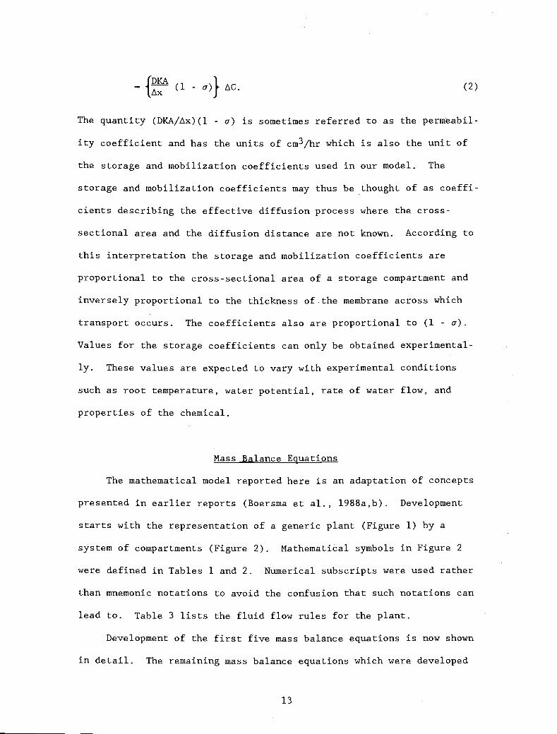
The quantity (DKA/x)(1 - a) is sometimes referred to as the permeabil-
ity coefficient and has the units of cm3/hr which is also the unit of
the storage and mobilization coefficients used in our model. The
storage and mobilization coefficients may thus be thought of as coeffi-
cients describing the effective diffusion process where the cross-
sectional area and the diffusion distance are not known. According to
this interpretation the storage and mobilization coefficients are
proportional to the cross-sectional area of a storage compartment and
inversely proportional to the thickness of.the membrane across which
transport occurs. The coefficients also are proportional to (1 - a).
Values for the storage coefficients can only be obtained experimental-
ly. These values are expected to vary with experimental conditions
such as root temperature, water potential, rate of water flow, and
properties of the chemical.
Mass Balance Equations
The mathematical model reported here is an adaptation of concepts
presented in earlier reports (Boersma et al., 1988a,b). Development
starts with the representation of a generic plant (Figure 1) by a
system of compartments (Figure 2). Mathematical symbols in Figure 2
were defined in Tables 1 and 2. Numerical subscripts were used rather
than mnemonic notations to avoid the confusion that such notations can
lead to. Table 3 lists the fluid flow rules for the plant.
Development of the first five mass balance equations is now shown
in detail. The remaining mass balance equations which were developed
THIS P
UBLICATIO
N IS O
UT OF D
ATE.
For mos
t curr
ent in
formati
on:
http:/
/exten
sion.o
regon
state.
edu/c
atalog

in a similar manner are in Appendix 1. Figure 2 shows the numbering
scheme of the compartments representing the various plant regions. The
subscripts on the fluid flows can also be used as indicators for the
intercompartmental parameter for chemical transport. In the mathemati-
cal model the term "mass transport" is used to describe the transport
of chemical due to diffusion, advection, and/or active processes. This
was done in accordance with concepts of transport modelling (Seagrave,
1971). The approach lumps diffusion, passive advection, and active
first-order transport together in one general first-order term. Lack
of knowledge generally precludes the separation of the active and
passive processes, especially at the macroscale.
Soil Compartment
Beginning with the soil compartment (Figure 2) the first mass
balance equation is:
d[e V1(l + B1) C1] instantaneous time rate of change
dt= of free phase plus reversibly bound
chemical mass (pg/h)
rate of diffusion of chemical- A(C1 - C0) mass across the soil/root
0 interface (pg/h)
rate of mass transport across thesoil/root interface (pg/h)
rate of irreversible first orderloss processes operating in thesoil compartment (pg/h)
14
(3)
where the subscript -1 identifies the soil compartment and 0 is the
root free space.
The relationship between the concentration of chemical in the free
phase and its mass in the soil compartment is
- Q0 C]
- A1 M.THIS P
UBLICATIO
N IS O
UT OF D
ATE.
For mos
t curr
ent in
formati
on:
http:/
/exten
sion.o
regon
state.
edu/c
atalog

M1 = f(l + B1) V1 C1 (jig) (4)
aLx0
-1,0 V0(l + B0)(1/h) (8)
where al,l characterizes the total chemical transport from the soil
compartment (compartment -1) to the root-free space and a1,o charac-
terizes diffusive transport from the root-free space back to the soil
compartment.
Free Space of the Roots
The second mass balance equation defines the time rate of change
of the chemical mass in the free space of the root cortex. The trans-
port pathways into and out of this region are shown in Figure 2.
15
and similarly in the compartment simulating the free space of the
cortex
M0 = (1 + B0) V0 C0 . (pg) (5)
Solving equation (4) for C1 in terms of M1 and solving equation (5)
for C0 in terms of MO with subsequent substitution of C1 and C0 into
equation (3) yields
dM-1 = a11 M
-1+ a10 N0 (6)
which is the first mass balance equation. The matrix elements ai,l
and al,o are defined by
(DDAO)
Ix0
Ia11 = -[ V(1 + B) + lj(1/h) (7)
D0 A0
THIS P
UBLICATIO
N IS O
UT OF D
ATE.
For mos
t curr
ent in
formati
on:
http:/
/exten
sion.o
regon
state.
edu/c
atalog

Compound is assumed to be brought into this region by advective flow
due to the transpiration stream and by diffusion which occurs in re-
sponse to gradients which exist between the soil solution, or nutrient
solution, and the free space of the cortex. The compound may be either
passively (diffusion) or actively taken up by the cells of the cortex
which make up compartment 1. Forward and backward transport coeff i-
cients with dimensions of volume rate of flow (cm3/hr) define transport
into and out of storage. If the uptake of compound by the exterior
root cell stem compartment is by diffusion only, then Q is the
product of a membrane diffusion coefficient (cm2/hr) and an effective
interfacial area (cm2) divided by a characteristic membrane thickness
(cm). The result may be multiplied by a partition coefficient and a
transmission coefficient to allow gradients to exist across the cortex
cells and free space at equilibrium conditions. Backward transport
coefficients are similarly defined.
Putting the currently recognized process and transport rules to-
gether in a linear model obtains
Dx:O (C1 - C0)
+ Q0 C1
ST- Qf0 C0
STbo
Cl
instantaneous time rate of change offree phase plus reversibly boundchemical mass in the free space ofthe cortex (pg/h)
rate of diffusion of chemical massacross the soil/ root interface (pg/h)
rate of mass transport across thesoil/root interface (pg/h)
rate of first-order loss due tostorage (pg/h)
rate of first-order gain due tomobilization from storage (pg/h)
16
dH0
dt
THIS P
UBLICATIO
N IS O
UT OF D
ATE.
For mos
t curr
ent in
formati
on:
http:/
/exten
sion.o
regon
state.
edu/c
atalog

- Q1(1 - a1) C0 rate of mass transport acrossthe endodermis (pg/h)
D1 A1 rate of diffusion of chemicalmass across the cortex/root
-
X1(C0 - C2)
xylem interface (pg/h)
- A0 M0 rate of all other first-orderirreversible processes in thefree space of the cortex (pg/h)
Define chemical masses in the compartments as follows:
M1 = (1 + B1) V1 C1
M2 = (1 + B2) V2 C2,
Solving equations (10) and (11) for C in terms. of M and substituting
for C..1, CO3 C1, and C2 into equation (9) yields the second mass
balance equation
17
dM0a02 M2 (pg) (12)= a01 M1 + a00 M0 + a01 M1 +
where the "matrix elements" are defined by
D0A0+
(1/h) (13)a01= 6 (1 + B1) V1
A0 D1 A1
[Do
QST+ Q1(1
-a1)
xo Ex1 fo
+A0 (1/h) (14)a00 =- (1 + B0) V0
ST
bo(1/hr) (15)a01
= (1 + B1) V1
D1 A1
Lx(1/h) (16)a02
= (1 + B2) V2
THIS P
UBLICATIO
N IS O
UT OF D
ATE.
For mos
t curr
ent in
formati
on:
http:/
/exten
sion.o
regon
state.
edu/c
atalog

Storage Volume of Root Cortex
The third mass balance equation defines the time rate of change of
chemical mass in the cells of the root cortex. Uptake of compound may
be by diffusion and/or active mass transport. The balance equation is
made up of three first-order processes:
dt
ST- Qf0 C0
+ b0C1
ST
[ boa11 =
- (1 + B1) V1 +
instantaneous time rate of change of freephase plus reversibly bound chemical massin the root cortex storage compartment (jig/h)
rate of first-order loss due to storage(pg/h)
rate of first-order gain due tomobilization from storage (pg/h)
rate of all other first-order irreveribleprocesses, including metabolism, in the
cell volume of the cortex (jig/h)
Chemical masses in the compartments were define earlier as follows:
M0= (1 + B0)V0C0 (5)
= (1 + B1)B1V1
Substitution for the two indicated concentrations yields
dM1
= a10 M0 + a11 M1
where the matrix elements are defined by
STQf0
a10= (1 + B V0
18
(17)
(20)
(10)
THIS P
UBLICATIO
N IS O
UT OF D
ATE.
For mos
t curr
ent in
formati
on:
http:/
/exten
sion.o
regon
state.
edu/c
atalog

Root Xylem Compartment
The fourth mass balance equation defines the time rate of change
of mass in the compartment simulating the root xylem. The transport
pathways and processes into and out of this compartment are shown in
Figure 2. The flows are self explanatory.
The mass balance equation for the root xylem compartment is:
dt
D1A1(C0 - C2)
ST- Qf1 C2
ST+ bl
3
- 2M2
instantaneous time rate of changeof free phase plus reversibly boundchemical mass in the root xylemcompartment (pg/h)
rate of diffusion of chemical massacross the root/xylem interface(pg/h)
rate of mass transport from thecortex to the root xylem (pg/h)
D4 A4 rate of diffusion of chemical mass+
ix(C4 - C2) across the root phloem/root xylem
4 interface (pg/h)
+ Q4(l - a4) C4 rate of mass transport from rootphloem to root xylem (pg/h)
D2 A2 rate of diffusion of chemical mass
-(C2 - C5) across from root xylem adjacent stem
2 xylem interface (pg/h)
- Q2- - a2) C2 rate of mass transport from rootxylem to adjacent stem xylem (pg/h)
rate of first-order loss due tostorage (pg/h)
rate of first-order gain due tomobilization from root storage(pg/h)
rate of all other first-orderirreversible processes inroot xylem compartment (pg/h)
19
(21)
Define masses in the three compartments as follows:
(1 + B3) V3 C3 (pg) (22)
THIS P
UBLICATIO
N IS O
UT OF D
ATE.
For mos
t curr
ent in
formati
on:
http:/
/exten
sion.o
regon
state.
edu/c
atalog

M4 (1 + B4) V4 C4
M5 (1 + B5) V5 C5
The fourth mass balance equation for the time rate of change of mass
2/dt is obtained by solving each of equations (22), (23), and (24)
for its compartment concentration Cj in terms of its compartment mass
Mi, substituting the result into equation (21), and collecting common
20
terms. The result is:
M0 + a22 M2 + a23
D1 A1
M3 + a24 M4
+ Q2(1 - a2)
+ a25 M5
ST+ Qf1
(25)
(26)
(27)
(28)
(29)
(30)
=
where
a20 =
a2,2=
a23=
a24
a25=
+ Q1(1 - a1)Lx1
-
V1(l + B1)
D1A1 D4A4 D2A2
+Ax4
+V2(l+B2)
ST
1
V3(1 + B3)
D4 A4+ Q(l - a4)
V4(l + B4)
D2 A2
AX2
V5(l + B5)
THIS P
UBLICATIO
N IS O
UT OF D
ATE.
For mos
t curr
ent in
formati
on:
http:/
/exten
sion.o
regon
state.
edu/c
atalog
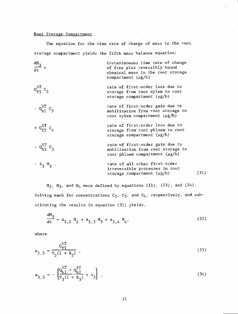
Root Storage Compartment
The equation for the time rate of change of mass in the root
storage compartment yields the fifth mass balance equation:
STQf1 C2
QST rate of first-order gain due tobl 3 mobilization from root storage to
root xylem compartment (jig/h)
ST+ Qf2 C4
ST
- b23
- X3
M2, M3, and M4 were defined by equations (11), (23), and (24).
Solving each for concentrations C2, C3, and C4, respectively, and sub-
stituting the results in equation (31) yields,
dM.
= a32 M2 + a33 M3 + a34 M4,
where
STQf1
a23- V2(l + B2)
,ST ST
Ibl + b2a33- 1V3(1 + B3) +
instantaneous time rate of changeof free plus reversibly boundchemical mass in the root storagecompartment (jig/h)
rate of first-order loss due tostorage from root xylem to rootstorage compartment (jig/h)
rate of first-order loss due tostorage from root phloem to rootstorage compartment (jig/h)
rate of first-order gain due tomobilization from root storage toroot phloem compartment (jig/h)
rate of all other first-orderirreversible processes in rootstorage compartment (jig/h)
21
(31)
dM3
dt
THIS P
UBLICATIO
N IS O
UT OF D
ATE.
For mos
t curr
ent in
formati
on:
http:/
/exten
sion.o
regon
state.
edu/c
atalog

STQf2
a34- V4(1 + B4)
System of Equations
The remaining 19 mass balance equations with corresponding matrix
elements were derived in a similar manner. The complete listing of all
24 mass balance equations is given in Appendix 1. The total chemical
mass in each compartment is defined for i = 6,7,...22, by
M. = (1 + B.) V. C.. (36)1 1 1 1
The possibility of loss of mass due to volatilization from leaves is
included by stating:
D Arate of loss CH 11
'H C Cvia volatilization - - x c 18 - air
where H0 is the dimensionless Henry law constant for the chemical
compound being modeled, DCH (cm2/h) is the effective chemical diffusion
coefficient of the compound in the boundary layer over the leaf sur-
face, Cair (pg/g) is the concentration of the chemical compound in the
mixed air outside the boundary layer, Lxll (cm) is the thickness of the
boundary layer, and All (cm2) is the effective area of volatilization.
Rules, similar to equation (37), were also written for leaves 2 and 3.
Equation (37) allows communication with the atmosphere and incorpora-
tion of atmospheric conditions such as wind speed, and air temperature,
and relative humidity.
(35)
(37)
22
THIS P
UBLICATIO
N IS O
UT OF D
ATE.
For mos
t curr
ent in
formati
on:
http:/
/exten
sion.o
regon
state.
edu/c
atalog

23
Solution Method
The complete system of 24 differential equations in 24 unknowns
can be written in matrix form as
dM= A + (38)
with initial conditions summarized as
(o) =(39
where M is the 24 x 1 vector of unknown masses at time t, S is the 24 x
1 vector of sources which may have nonzero entries at positions 14, 17,
and 20, A is the 24 by 24 irreducible transport-transfer matrix, which
is real, weakly diagonally dominant, has negative diagonal entries,
and whose off diagonal entries are either positive or zero (Varga,
1962), and M0 is the 24 x 1 vector of initial chemical masses.
The system of equations given by equation (38) is linear and has
constant coefficients, over the arbitrary slice TL to T hours. As
such this system has a unique continuous solution vector M(t) (Boyce
and DiPrima, 1965). Each element Mi(t) of M(t) is itself a linear
combination of at most 24 elementary exponential functions. Because
assignment of appropriate weighting factors is not practical with
current knowledge, we chose to approximate the solution numerically.
The method outlined below is now enjoying a renewed interest and usage
due to the availability of microcomputers with large storage, high
speed, and double precision arithmetic. It is a useful method for
large, sparse, arrays with constant coefficients such as frequently
arise in biological and control systems.
THIS P
UBLICATIO
N IS O
UT OF D
ATE.
For mos
t curr
ent in
formati
on:
http:/
/exten
sion.o
regon
state.
edu/c
atalog

Define the matrix exponential function, sometimes called the
fundamental solution matrix, to be
At (AYee 'ei 2!
This series serves as the basis for the numerical solution method,
although it is useful for computing only for small values of time t
(Boyce and DiPrima, 1965), where I is the identity matrix. Boyce and
DiPrima (1965) prove many important properties about this matrix expo-
nential function, such as
Atde Ati) differentiation: = A edt
commutation:
commutation:
Rewrite equation (38) as
dN
and matrix multiply left by eAt, the inverse matrix of eAt (Boyce and
DiPrima, 1965), and recast the system into the form
d(eAt M)
dt-At
e S.
24
At AtAe =e A (42)
-1 At At -1A e =e A . (43)
Next, superimpose on the time line a lattice of points t0, t], t2,.
so that t0 = 0, t1 Lt, t2 = 2At, t3 = 3t .....then multiply both
sides of equation (45) by the differential dt, and integrate both sides
between the two time points tn, tn+l, to obtain:
THIS P
UBLICATIO
N IS O
UT OF D
ATE.
For mos
t curr
ent in
formati
on:
http:/
/exten
sion.o
regon
state.
edu/c
atalog

-At -Atn+1 n
e M(t ) - e M(t )- n+l - n
-At -At-1 n+1 n=-A (e -e )S
Ati
Matrix multiply left both sides of equation (46) by en+
to obtain
the explicit recursion formula
Ait -1 kAtM(t )=e M(t)-A (I-e )S- n+l - n
Note that no approximation has as yet been made. Equation (47) is an
exact solution of the original differential system, but the solution
consists of M evaluated only on a discrete set of time points. Define
the constant vector W via the formula
= -1 ALtW A (I-e )S
Clearly, on the discrete set of time points to,tl,t2.
AtM(t )=e M(t)+W- n+l - n -
which is a 24-dimensional, first-order, nonhomogeneous, difference
system (Varga, 1962; Jacquez, 1972).
Mathematical induction shows that the unique solution to system
(49) is
At nAAt n AAt -1M(t ) = (e ) M + (I - e ) (I - (e ) )W- n o -
for n = 1,2,3...
Because et is a positive 24 x 24 array with a spectral radius
(modulus of the maximum eigenvalue) less than 1, eAAt is said to be a
convergent array since, as n -+ (et)n - Z, the array of zero
elements (Varga, 1962). It can be shown that
25
THIS P
UBLICATIO
N IS O
UT OF D
ATE.
For mos
t curr
ent in
formati
on:
http:/
/exten
sion.o
regon
state.
edu/c
atalog

urn M (t- nfl-co
which follows directly from equation (50).
Equation (49) is used for computational purposes. The approxima-
tion is made because et can only be computed to the double precision
limits of the computer. A useful method for carrying out the computa-
tion is to observe that
= -A1
26
(Ward, 1977, Moler and Van Loan, 1978).
The key to computing exp[At] to high precision is to first
compute exp[-At/N}, using the matrix exponential function definition
40 to the double precision limits of the computer. Next, compute
(exp[-At/N])l, the inverse-scaled exponential matrix function via the
classical LU factorization method. Lastly, raise exp[-AAt/N]1- to the
power N. Other scaling methods exist (Golub and Van Loan, 1983). Time
marching scheme (49) is a stable scheme in that any small perturbation
introduced into the data at some time tk > 0, propagates in a bounded
fashion as time exceeds tk, arbitrarily large (Varga, 1962).
Effective Concentrations
In most experimental situations it is difficult, if not impossi-
ble, to sample the phloem, xylem, or storage compartments individually
At -Ant -AAtAAt
eN N N N-i
(e ) = ((e ) ) =N -iN
[(e ) I (51)
where N is chosen to
-a. .At
be a power of 2, just large enough so that
maxli24
11
}<1(52)
N
THIS P
UBLICATIO
N IS O
UT OF D
ATE.
For mos
t curr
ent in
formati
on:
http:/
/exten
sion.o
regon
state.
edu/c
atalog

to determine concentrations (g/cm3) at points in time. For example,
when evaluating accumulation by leaves it is usually most convenient to
harvest groups of leaves and obtain an average concentration (DPM/g) or
(jg/g) for the group. An average or "effective tissue concentration"
can then be obtained by dividing the chemical mass present by the wet
mass of tissue (pg/g). An effective volume-based concentration (,ag/cm3)
can be obtained when the density is known. Assuming that the density
of most plant parts of young soybean plants is 1/cm3, effective concen-
trations (jg/cm3) are defined as below. In the definition, (t) indi-
cates concentration at time t and OA indicates the overall average
concentration for the indicated plant part:
in the roots,
4 4
C (t) . M./. V.roots i=0 1 i=0 1
in the individual stem parts,
7 7
C (t) = .E M./.> V.stem b i=5 1 i=5 1
10 10
C (t) = . M./. V.;stem in i=8 1 i=8 1
13 13
C (t)= .> M/. V.;stemt ill ii=ll 1
in the stem,
13 13
C (t)= M/ V.;stem OA i=5 i i=5 1
iv) in the individual leaf clusters,
27
THIS P
UBLICATIO
N IS O
UT OF D
ATE.
For mos
t curr
ent in
formati
on:
http:/
/exten
sion.o
regon
state.
edu/c
atalog
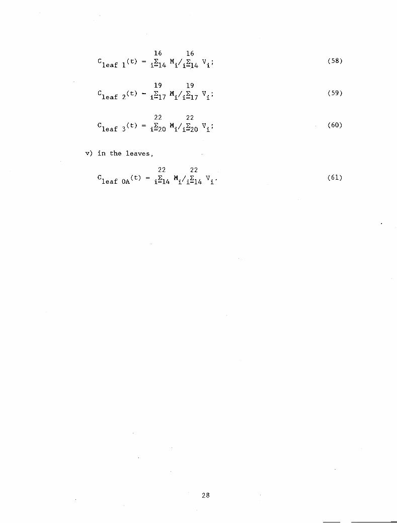
16 16C (t) = . M./. V.leaf 1 i=14 1 i=14 1
19 19C1f 2(t) = . M./ V
i=17 1 1=17
22 22C1f 3(t)
= i2O M./ V1 i=20
v) in the leaves,
22 22C1f (t) = M / V..
OA i=l4 i i=14 1
28
THIS P
UBLICATIO
N IS O
UT OF D
ATE.
For mos
t curr
ent in
formati
on:
http:/
/exten
sion.o
regon
state.
edu/c
atalog
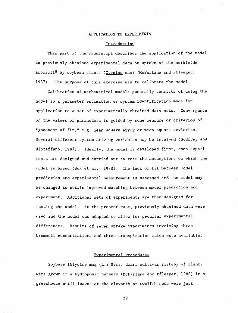
APPLICATION TO EXPERIMENTS
Introduction
This part of the manuscript describes the application of the model
to previously obtained experimental data on uptake of the herbicide
Bromacil® by soybean plants (Clycine max) (McFarlane and Pfleeger,
1987). The purpose of this exercise was to calibrate the model.
Calibration of mathematical models generally consists of using the
model in a parameter estimation or system identification mode for
application to a set of experimentally obtained data sets. Convergence
on the values of parameters is guided by some measure or criterion of
ttgoodness of fit," e.g. mean square error or mean square deviation.
Several different system driving variables may be involved (Godfrey and
diSteffano, 1987). Ideally, the model is developed first, then experi-
ments are designed and carried out to test the assumptions on which the
model is based (Box et al.,, 1978). The lack of fit between model
prediction and experimental measurement is assessed and the model may
be changed to obtain improved matching between model prediction and
experiment. Additional sets of experiments are then designed for
testing the model. In the present case, previously obtained data were
used and the model was adapted to allow for peculiar experimental
differences. Results of seven uptake experiments involving three
bromacil concentrations and three transpiration rates were available.
Experimental Procedures
Soybean [Glycine max (L.) Merr. dwarf cultivar Fiskeby v plants
were grown in a hydroponic nursery (McFarlane and Pfleeger, 1986) in a
greenhouse until leaves at the eleventh or twelfth node were just
29
THIS P
UBLICATIO
N IS O
UT OF D
ATE.
For mos
t curr
ent in
formati
on:
http:/
/exten
sion.o
regon
state.
edu/c
atalog

starting to develop. All lateral stems were removed as they initiated.
The nutrient solution was a modified, half-strength, Hoagland solution
(Berry, 1978) with a pH of 6.0 and electrical conductivity of 1.2 dS/ni.
Plants of similar size were transferred to the exposure chambers de-
scribed by McFarlane and Pfleeger (1987). Plants were acclimated for
three days to the conditions of the controlled environment prior to
adding 14C-labeled bromacil (U-14C6H13BrN2O2) to the nutrient solution.
The specific activity of the treatment stock was 6.16*106 Bq/mmole
bromacil as measured by liquid scintillation analysis and gas/liquid
chromatography. The treatment was started by the addition of the
amount of bromacil stock solution needed to obtain the desired
concentration in each plant exposure chamber. The concentrations used
in each of the three experiments are in Table 4 in addition to other
environmental parameters. Root exposure was monitored by periodically
sampling the hydroponic solution and analyzing for 14C activity. Each
sample was analyzed in triplicate and the analytical variation in
counting replicate samples was never larger than 3 percent of the mean.
The solution volume was maintained automatically at 6.5 liters by
replacing transpired water with nutrient solution but without bromacil.
Since bromacil uptake was approximately proportional to the transpira-
tion rate, chemical was lost at a faster rate from the solution with a
high transpiration rate than from one with a low transpiration rate.
Bromacil uptake was measured by periodically removing plants from
each chamber for determination of 14C concentration of the plant parts.
The stems were cut at the crown, the leaves removed, and fresh weights
were determined for leaves, stems, and roots. The tissues were freeze
dried. Roots and leaf tissues were ground to a powder, then subsamples
30
THIS P
UBLICATIO
N IS O
UT OF D
ATE.
For mos
t curr
ent in
formati
on:
http:/
/exten
sion.o
regon
state.
edu/c
atalog

Table 4. Environmental parameters and plant functions during uptaketest (BR0M3).
Parameter Units Value CV%
BROM1 BROM3 BROM5
Photosynthetic iimol/s m2 350 350 350Photon flux(PPF)*
Air Temperature C 23 23 23 2
Specific humidity g/m3 20 1
(low tr.) 16
(medium tr.) 12
(high tr.)Windspeed rn/s 0.6 15
Co2 mmol/m3 15.6 5
Transpiration(low) cm3/h plant 4.4 1.2 10
(medium) 7.6 5.7
(high) 7.0 9.5 7.3
Brornacil ,ag/cm3 0.528 0.180 0.058concentration ofbathing solution
*Light cycle on/off was 24/0 hours
were obtained and burned in a Packard 306 sample oxidizer. The CO2 was
collected and analyzed for 14C activity by liquid scintillation count-
ing. Stem material was not easily ground because of its fibrous
nature, therefore segments were selected from the lower, middle, and
top portions of each plant and oxidized without powdering. Attention
was given to the possibility of chemical loss during drying and as a
result of incomplete combustion in the oxidation step. Quality assur-
ance tests confirmed that less than 1 percent was lost in either
procedure.
31
THIS P
UBLICATIO
N IS O
UT OF D
ATE.
For mos
t curr
ent in
formati
on:
http:/
/exten
sion.o
regon
state.
edu/c
atalog

Transformation of bromacil was tested by evaluation of thin-layer
chromatographs made from plant extracts and from the hydroponic solu-
tion. Only bromacil was found in the nutrient solution and roots, but
about 5 percent of the 1-4C activity in the leaves was determined to be
associated with another chemical. This result was also found in other
studies (McFarlane et al., 1987). Since this was a small contribution
to the total -4C activity, and since all the bromacil was accounted for
in this study, it was assumed that the results presented on the basis
of DPM are an accurate description of the movement patterns of bromacil
in the test plants.
Three experiments with bromacil uptake were conducted, each with
some different aspect in timing, dosing concentration, or experimental
conditions (Table 4). The knowledge gained from the first experiment
(BROM1) led to the design of the second (BROM3) which included three
exposure chambers, each with a different transpiration rate. In the
final experiment (BROM5) bromacil was periodically added to each
chamber so that the concentration in the nutrient solutions remained
approximately constant throughout the exposure. In the first two
tests, individual leaves, stems, and root segments were analyzed. In
the last test, samples were pooled and subsamples representing plant
regions were analyzed.
Since two types of experiments were conducted, namely, one with
decreasing bromacil concentration and one with constant bromacil con-
centration, the mathematical model was formulated in a manner which
allowed either condition to exist in the simulation.
Results of the three experiments include measurements of transpi-
ration rates, leaf areas, wet mass of harvested plant parts (Table 5),
32
THIS P
UBLICATIO
N IS O
UT OF D
ATE.
For mos
t curr
ent in
formati
on:
http:/
/exten
sion.o
regon
state.
edu/c
atalog

Table 5. Measured transpiration rates, leaf areas, and wet masses ofroots, stems, and leaves for three experiments with differentbromacil concentrations. The data shown are averages ofseveral measurements obtained during an experimental period of220 hrs for BROM5, 55 hrs for BROM3, and 72 hrs for BROM1.Number in parenthesis following leaf area and mass of wet plantmaterial is estimated standard error (ese).
33
and concentrations of radio-labeled bromacil in the separately harvested
plant parts as a function of exposure time (Table 6). The transpiration
rates shown in Table 5 were obtained by measuring the volume of water
lost during measurement intervals. Table 5 indicates that the plants of
the BROM3 experiment were about twice as large as those of BROM1 and
BROM5.
The BROM5 experiment had the lowest bromacil concentration. The
measured concentration of radio-labeled bromacil in the tank was
3250 DPM/cm3, which corresponds to 0.058 pg bromacil/cm3 solution
(Table 4). The BROM3 experiment used an initial bromacil concentration
which was 3.1 times higher (0.180 pg/cm3) and BROM1 used an initial
bromacil concentration which was 9.1 times higher (0.528 pg/cm3).
Experiment Leaf area Transp rateWet mass of plant parts
Roots Stems Leaves
cm2 cm3/cm2 hr g g g
765 (103) 2.61 x l0 24.7 (3.5) 4.5 (0.8) 16.7 (2.9)BROM5 725 (122) 7.82 x l0 31.1 (9.3) 6.5 (1.4) 17.3 (4.0)
825 (116) 8.85 x l0 31.5 (6.0) 6.6 (1.1) 19.9 (3.7)
Stems plus leaves
1578 (250) 2.77 x l0 45.5 (6.7) 71.2 (7.8)BROM3 1761 (261) 4.32 x l0 56.5 (9.3) 81.4 (9.9)
1794 (160) 5.26 x l0 47.9 (11.8) 77.0 (8.2)
BROM1 845 (110) 8.65 x l0 30.0 (6.3) 6.1 (0.6) 21.3 (2.1)
THIS P
UBLICATIO
N IS O
UT OF D
ATE.
For mos
t curr
ent in
formati
on:
http:/
/exten
sion.o
regon
state.
edu/c
atalog
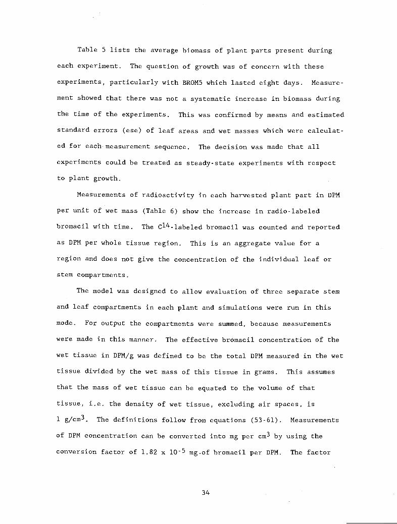
Table 5 lists the average biomass of plant parts present during
each experiment. The question of growth was of concern with these
experiments, particularly with BROM5 which lasted eight days. Measure-
ment showed that there was not a systematic increase in biomass during
the time of the experiments. This was confirmed by means and estimated
standard errors (ese) of leaf areas and wet masses which were calculat-
ed for each measurement sequence. The decision was made that all
experiments could be treated as steady-state experiments with respect
to plant growth.
Measurements of radioactivity in each harvested plant part in DPM
per unit of wet mass (Table 6) show the increase in radio-labeled
bromacil with time. The C14-labeled bromacil was counted and reported
as DPM per whole tissue region. This is an aggregate value for a
region and does not give the concentration of the individual leaf or
stem compartments.
The model was designed to allow evaluation of three separate stem
and leaf compartments in each plant and simulations were run in this
mode. For output the compartments were summed, because measurements
were made in this manner. The effective bromacil concentration of the
wet tissue in DPM/g was defined to be the total DPM measured in the wet
tissue divided by the wet mass of this tissue in grams. This assumes
that the mass of wet tissue can be equated to the volume of that
tissue, i.e. the density of wet tissue, excluding air spaces, is
1 g/cm3. The definitions follow from equations (53-61). Measurements
of DPM concentration can be converted into mg per cm3 by using the
conversion factor of 1.82 x lO mg.of bromacil per DPM. The factor
34
THIS P
UBLICATIO
N IS O
UT OF D
ATE.
For mos
t curr
ent in
formati
on:
http:/
/exten
sion.o
regon
state.
edu/c
atalog

Table 6. Bromacil concentrations in DPM per gram wet biomass.
BROM5
Low Medium HighTime Roots Stems Leaves Roots Stems Leaves Roots Stems Leaves
(hr) DPM/g wet mass
8 5,149 3,654 507 5,537 9,495 2,079 5,763 5,233 3,432
26 7,058 11,864 3,473 6,767 9,565 10,221 7,065 10,12 14,93550 8,315 18,634 7,262 22,303 22,883 8,239 25,086 25,641
122 36,793 26,293 12,521 33,252 49,999 10,485 32,684 88,247145 16,094 35,815 30,148 15,039 30,124 61,317 13,950 38,093 106,952169 18,041 36,512 35,009 18,652 38,244 71,081 16,993 31,523 122,381193 19,876 60,609 33,155 19,139 32,377 67,277 16,253 37,689 133,190218 51,010 42.686 41.497 21,234 43,715 140,209
BROM3Low Medium High
Time Roots Shoots Roots Shoots Roots Shoots
(hr) DPM/g wet mass
3.0 12,616 536 15,042 631 12,521 1,792
7.0 15,651 2,725 14,641 . 1,978 13,237 6,06015.0 14,550 6,029 17,779 7,587 13,926 14,11923.0 16,218 10,239 21,452 13,162 15,683 18,23631.0 16,614 14,700 21,731 15,803 17,046 29,237
39.0 20,542 26,926 19,097 19,661 16,876 32,06847.0 21,382 25,527 26,211 21,601 21,085 27,77055.0 17,719 29.813 ** 33.074 18,006 36,435
BROM1
Stems Leaves
(hr) DPM/g wet mass
0.0 31,625 0.0 0.0 0.0 0.0 0.0 0.0 0.0
1.0 29,186 24,737 11,158 7,002 4,667 904 1,171 837
4.0 27,820 33,009 32,563 29,252 17,878 14,817 12,808 14,929
8.0 26,383 32,007 47,592 42,421 31,172 43,027 40,659 58,76224.0 25,750 40,982 62,247 64,403 48,477 128,911 107,338 81,50548.0 24,200 44,497 86,676 86,590 90,527 259,725 254,319 414,12772.0 22.175 52,554 85,225 81 675 88.982 370.528 368,820 628,669
Time Tank Roots Bottom Mid Top Bottom Mid Top
35
THIS P
UBLICATIO
N IS O
UT OF D
ATE.
For mos
t curr
ent in
formati
on:
http:/
/exten
sion.o
regon
state.
edu/c
atalog

follows from:
0.05834 (pg/cm3)/3200 (DPM/cm3) 1.82 x lO (mg/DPM).
Qualitative Overview of Results
An initially very rapid increase in concentration occurred in the
roots (Figure 3) with all experiments, followed by a slower rate of
increase which remained nearly constant with time. The rapid increase
during the first few hours of exposure was attributed to the filling of
the free space of the root cortex with the bathing solution, with a
concurrent rapid entry of solute into the cortex cells. The rapid
permeation occurred as the transpiration stream drew in the bathing
solution immediately upon exposure to the solution. This rapid in-
crease indicates a large value for the storage coefficient during the
early part of the uptake process with smaller values during the time
following the initial loading.
Concentrations of the stem compartments of the BROM5 and BROM3
experiments (Figure 4) did not show the rapid initial increase that was
found in the root compartments. However, a rapid increase in concen-
tration did occur with the BROM1 experiment, with plants exposed to the
high concentration of bromacil in the bathing solution (Table 4). The
increase in stem concentrations was nearly linear for all three experi-
ments during the first 50 hours of exposure. Concentrations in the
stem compartments were higher than in the root compartments, suggesting
that storage coefficients for the stem compartments were higher than
for the root compartments and that the ratio of forward storage coeffi-
cient (Qb) to backward storage coefficient (Q) was higher.
36
THIS P
UBLICATIO
N IS O
UT OF D
ATE.
For mos
t curr
ent in
formati
on:
http:/
/exten
sion.o
regon
state.
edu/c
atalog

60
- 50CO0
><
(1)
(I)
E40ci)
ECTi
0)
0
C
.I-JCci)00o 10 Transpiration
Rate
o LowMedium
o High
37
20 40 60 80
Time of Exposure (hrs)
Figure 3. Measured bromacil concentrations in the root compartments.Details of the experimental procedures are in the text. The
curves shown were drawn by hand to emphasize trends inincrease in concentration. The graphs show an initial rapidrise in concentration, followed by a linear increase withtime.
THIS P
UBLICATIO
N IS O
UT OF D
ATE.
For mos
t curr
ent in
formati
on:
http:/
/exten
sion.o
regon
state.
edu/c
atalog

100
C)80
60E
C)
0-40
0I-
I-C0C
200
38
0
Brom 1
X 5Low+ 5MedG 5High
3LowA 3Med
3High
o iBottomz iMido hop
S
. Brom3U
0 20 40 60 80Time of Exposure (hrs)
Figure 4. Measured bromacil concentrations in the stem compartments.Details of the experimental procedures are in the text.Curves were drawn by hand to emphasize trends in increase inconcentrations. The graphs show a linear increase in con-centration during the exposure period.
THIS P
UBLICATIO
N IS O
UT OF D
ATE.
For mos
t curr
ent in
formati
on:
http:/
/exten
sion.o
regon
state.
edu/c
atalog
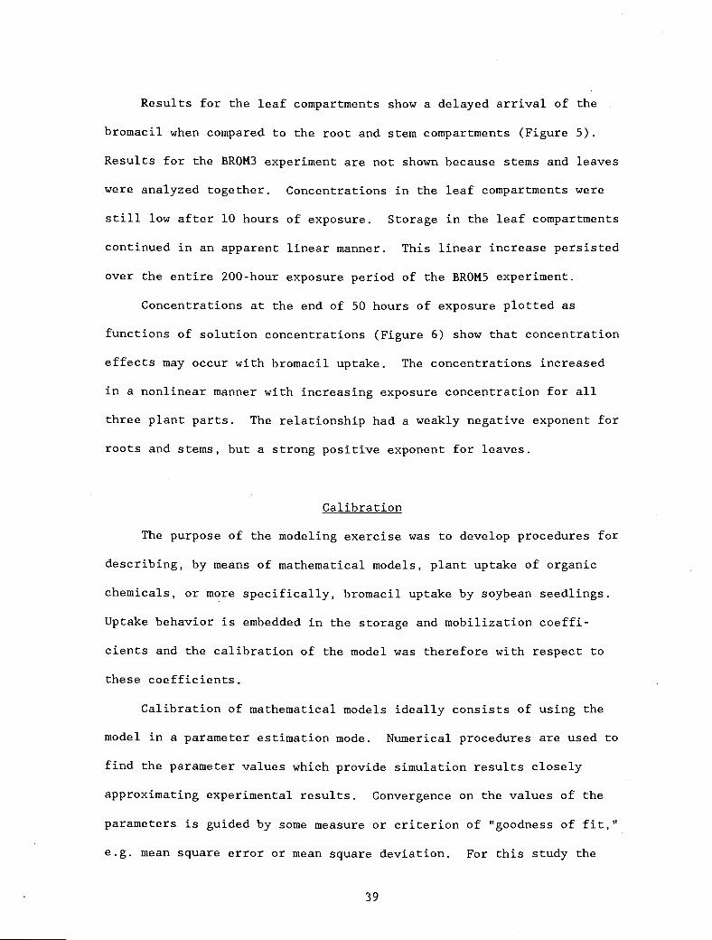
Results for the leaf compartments show a delayed arrival of the
bromacil when compared to the root and stem compartments (Figure 5).
Results for the BROM3 experiment are not shown because stems and leaves
were analyzed together. Concentrations in the leaf compartments were
still low after 10 hours of exposure. Storage in the leaf compartments
continued in an apparent linear manner. This linear increase persisted
over the entire 200-hour exposure period of the BROM5 experiment.
Concentrations at the end of 50 hours of exposure plotted as
functions of solution concentrations (Figure 6) show that concentration
effects may occur with bromacil uptake. The concentrations increased
in a nonlinear manner with increasing exposure concentration for all
three plant parts. The relationship had a weakly negative exponent for
roots and stems, but a strong positive exponent for leaves.
Calibration
The purpose of the modeling exercise was to develop procedures for
describing, by means of mathematical models, plant uptake of organic
chemicals, or more specifically, bromacil uptake by soybean seedlings.
Uptake behavior is embedded in the storage and mobilization coeffi-
cients and the calibration of the model was therefore with respect to
these coefficients.
Calibration of mathematical models ideally consists of using the
model in a parameter estimation mode. Numerical procedures are used to
find the parameter values which provide simulation results closely
approximating experimental results. Convergence on the values of the
parameters is guided by some measure or criterion of "goodness of f it,"
e.g. mean square error or mean square deviation. For this study the
39
THIS P
UBLICATIO
N IS O
UT OF D
ATE.
For mos
t curr
ent in
formati
on:
http:/
/exten
sion.o
regon
state.
edu/c
atalog
100
E
0) 0
5000
40-0
30-0C0o 20-
Brom 1, Leaves
o Bottom LeafA Middle Leafo Top Leaf
20
40
40 60 80
20 40 60
Time of Exposure (hrs)
Figure 5. Measured bromacil concentrations in the leaf compartmentsfor the BROM1 and BROM5 experiments. Curves were drawn byhand to emphasize trends. Results suggest a linear rate ofuptake in these experiments with constant transpirationrates.
80
600-
500 -
0';< 300-(I)
200-
THIS P
UBLICATIO
N IS O
UT OF D
ATE.
For mos
t curr
ent in
formati
on:
http:/
/exten
sion.o
regon
state.
edu/c
atalog
C)Q1><
(I)
C/) 250-
E
)2OO
- 150-ct
0-4-I
100-
0oh 012 03 014 015 0.6
Bromacil Concentration Qig/cm3)
Figure 6. Concentration at 50 hrs of exposure as a function of solu-tion concentration.
41
THIS P
UBLICATIO
N IS O
UT OF D
ATE.
For mos
t curr
ent in
formati
on:
http:/
/exten
sion.o
regon
state.
edu/c
atalog

number of data points was not sufficient to follow this ideal proce-
dure. Since model development is a recent activity, this circumstance
is not unusual. Godfrey and diSteffano (1987) recently addressed the
problem and describe procedures for finding parameters using incomplete
data sets.
According to recommended procedures, the data of the uptake exper-
iments were first used to gain insight into the process to be modeled.
This was initiated earlier in the manuscript with a qualitative analy-
sis of the experimental results. This analysis was also used to set
initial values of the parameters. Thus an iterative procedure, guided
at each step by comparison of simulation and experimental data, was
used to systematically adjust Qfi and Qbj values until agreement be-
tween simulation and measured results was obtained. About 50 sets of
simulations were needed to arrive at the set of storage coefficients
which gave acceptable agreement with experimental results. Providing
mathematical proof that the storage coefficients obtained in this
manner are unique is not possible. Another set of values, different
from those shown which would give an equally good fit to the data, may
exist.
UTAB 4.6 is a medium-resolution model. As such, it requires
values for a large number of geometric and physiologic parameters which
must be obtained before calibration with respect to storage coeffi-
cients can begin. Values of the parameters were chosen on the basis of
a "normalized" plant with a total leaf area of 1000 cm2 and then scaled
according to measured plant sizes. Leaf areas were in the range 800 to
1,800 cm2 (Table 2). This approach was used in earlier reports
42
THIS P
UBLICATIO
N IS O
UT OF D
ATE.
For mos
t curr
ent in
formati
on:
http:/
/exten
sion.o
regon
state.
edu/c
atalog
(Boersma et al., 1988a,b,c) and values for anatomical features of
soybean plants were derived from these reports.
Volumes of Compartments
Literature data and experimental results indicated that the gener-
ic soybean plant with a leaf area of 1,000 cm2 would have a root volume
of 25 cm3, a stem volume of 6 cm3, and a leaf volume of 25 cm3
(Boersma, 1988a). The experimental plants corresponded approximately
to these values in terms of ratios and absolute values (Table 5). The
next step in setting up the data base for simulation was to obtain
volumes of all compartments of the model for each experiment. The
procedure for doing so is detailed by Table 7. The example shown in
Table 7 is for BROM5, medium-transpiration rate. The first step was to
change from wet mass to volume, based on the assumption of a tissue
density excluding air spaces equal to 1 g/cm3. The first column in
Table 7 shows the aggregate volume for each plant part of the normal-
ized plant, i.e. 25 cm3 for the roots, 6 cm3 for the stems, and 25 cm3
for the leaves. The second column shows the percent of each of these
volumes occupied by subcompartments. These percentages were chosen
from literature reports. The root was divided into the region outside
the endodermis (cortex) and the region inside the endodermis (xylem +
phloem + storage). Seventy-five percent was allocated to the cortex
and 25 percent to the stele. Then volumes of cortex and stele were
further subdivided. Of the cortex volume, 85 percent was allocated to
cell volume and 15 percent to apparent free space. The stele was sub-
divided into 4 percent xylem, 93 percent storage, and 3 percent phloem.
43
THIS P
UBLICATIO
N IS O
UT OF D
ATE.
For mos
t curr
ent in
formati
on:
http:/
/exten
sion.o
regon
state.
edu/c
atalog

Table 7. Basis for calculating the compartment volumes of the experi-mental plants. The example shown is BROM5, medium transpira-tion rate.
44
Compartment name and numberBasevolume
Fraction tocompartment
Basevolumes
VolumesBROM5(med.)
ROOTcm325
cm3 cm3
Root apparent free space (0) 0.75 0.15 2.813 3.499
Root cortex cells (1) 0.85 15.938 19.826
Root xylem (2) 0.25 0.04 0.250 0.311
Root storage (3) 0.93 5.813 7.231
Root phloem (4) 0.03 0.188 0.233
25.000 31.160
STEM 6
Bottom stem xylem (5) 0.735 0.04 0.176 0.191
Bottom stem storage (6) 0.93 4.101 4.443
Bottom stem phloem (7) 0.03 0.132 0.143
Mid stem xylem (8) 0.182 0.04 0.044 0.047
Mid stem storage (9) 0.93 1.016 1.100
Mid stem phloem (10) 0.03 0.033 0.035
Top stem xylem (11) 0.083 0.04 0.020 0.0217
Top stem storage (12) 0.93 0.463 0.5047
Top stem phloem (13) 0.03 0.015 0.0162
6.000 6.500
LEAF 25
Leaf cluster 1 xylem (14) 0.5 0.01 0.125 0.087
Leaf cluster 1 storage (15) 0.98 12.250 8.477
Leaf cluster 1 phloem (16) 0.01 0.125 0.087
Leaf cluster 2 xylem (17) 0.3 0.01 0.075 0.052
Leaf cluster 2 storage (18) 0.98 7.350 5.086
Leaf cluster 2 phloem (19) 0.01 0.075 0.052
Leaf cluster 3 xylem (20) 0.2 0.01 0.050 0.035
Leaf cluster 3 storage (21) 0.98 4.900 3.391
Leaf cluster 3 phloem (22) 0.01 0.050 0.035
25.000 17.300
THIS P
UBLICATIO
N IS O
UT OF D
ATE.
For mos
t curr
ent in
formati
on:
http:/
/exten
sion.o
regon
state.
edu/c
atalog

Stem volume was allocated as follows: 73.5 percent to bottom stem
segment, 18.2 percent to middle stem segment, and 8.3 percent to upper
stem segment. The volume of each stem segment was divided into 3
percent for phloem, 4 percent for xylem, and 93 percent for storage.
Total leaf volume was divided into 50 percent, 30 percent, and 20
percent to lower, middle, and upper leaf, respectively. Each of these
volumes was divided into 1 percent phloem, 1 percent xylem, and 95
percent storage.
The volumes used for simulation were then calculated by scaling
the base values from Table 7 in proportion to volumes derived from
measured plant mass (Table 5) using linear scaling. For example, with
the medium transpiration rate of BROM5 the mean root mass was 31.1 g
(Table 5). The volumes of root compartments (labeled 0 through 4) were
obtained by multiplication of the base volume of root compartment shown
in Table 7 by the quotient (31.1/25.0 = 1.244). This yielded the root
compartment volumes shown in the last column in Table 4. The sum of
these volumes should be 31.1 cm2. The scale factor for the stem com-
partments was (6.5/6.0 = 1.083), and (17.3/25 0.692) for the leaf
compartments. The same procedure was used to obtain volumes for the
other experiments. Table 8 summarizes the other geometric parameters
used in the UTAB 4.6 simulation runs.
Chemical and Physical Parameters
Information available for bromacil suggested setting sorption
parameters, first-order irreversible loss process param;ters, and
reflection coefficients all equal to zero. This information must be
45
THIS P
UBLICATIO
N IS O
UT OF D
ATE.
For mos
t curr
ent in
formati
on:
http:/
/exten
sion.o
regon
state.
edu/c
atalog
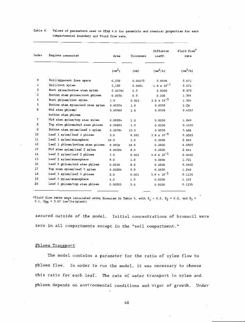
Table 8. Values of parameters used in UTAB 4.6 for geometric and chemical properties for each
compartmental boundary and fluid flow rate.
Diffusion Fluid flow*
secured outside of the model. Initial concentrations of bromacil were
zero in all compartments except in the "soil compartment.t'
Phloem Transport
The model contains a parameter for the ratio of xylem flow to
phloem flow. In order to run the model, it was necessary to choose
this ratio for each leaf. The rate of water transport in xylem and
phloem depends on environmental conditions and vigor of growth. Under
46
Index Regions connected Area Thickness coeff. rate
(cm2) (cm) (cm2fh) (cm3/h)
0 Soil/apparent free space 6,350 0.00375 0.0036 5.671
1 Soil/root xylem 3,180 0.0001 1.8 x io- 5.671
2 Root xylem/bottom stem xylem 0.00784 0.5 0.0036 6.975
3 Bottom stem phloem/root phloem 0.0055 0.5 0.036 1.304
4 Root phloem/root xylem 1.0 0.001 3.6 X i0 1.304
5 Bottom stem xylem/mid stem xylem 0.00504 1.0 0.0036 3.29
6 Mid stem phloem/ 0.00360 1.0
bottom stem phloem
0.0036 0.4537
7 Mid stem xylem/top stem xylem 0.00284 1.0 0.0036 1.249
8 Top stem phloem/mid stem phloem 0.00203 1.0 0.0036 0.1135
9 Bottom stem xylem/leaf 1 xylem 0.00784 10.0 0.0036 3.686
10 Leaf 1 xylem/leaf 1 phloem 5.0 0.001 3.6 X 1O 0.8505
11 Leaf 1 xylem/atmosphere 10.0 1.0 0.0036 2.835
12 Leaf 1 phloem/bottom stem phloem 0.0056 10.0 0.0036 0.8505
13 Mid stem xylem/leaf 2 xylem 0.00504 8.0 0.0036 2.041
14 Leaf 2 xylem/leaf 2 phloem 3.0 0.001 3.6 x 10 0.3402
15 Leaf 2 xylem/atmosphere 6.0 1.0 0.0036 1.701
16 Leaf 2 phloem/mid stem phloem 0.0036 8.0 0.0036 0.3402
17 Top stem xylem/leaf 3 xylem 0.00284 5.0 0.0036 1.249
18 Leaf 3 xylem/leaf 3 phloem 2.0 0.001 3.6 x l0 0.1135
19 Leaf 3 xylem/atmosphere 4.0 1.0 0.0036 1.135
20 Leaf 3 phloem/top stem phloem 0.00203 5.0 0.0036 0.1135
aFluid flow rates were calculated using formulas in Table 3, with f1 = 0.3, f2 0.2, and f3QTR = s.7 (cm3/hr/plant)
THIS P
UBLICATIO
N IS O
UT OF D
ATE.
For mos
t curr
ent in
formati
on:
http:/
/exten
sion.o
regon
state.
edu/c
atalog
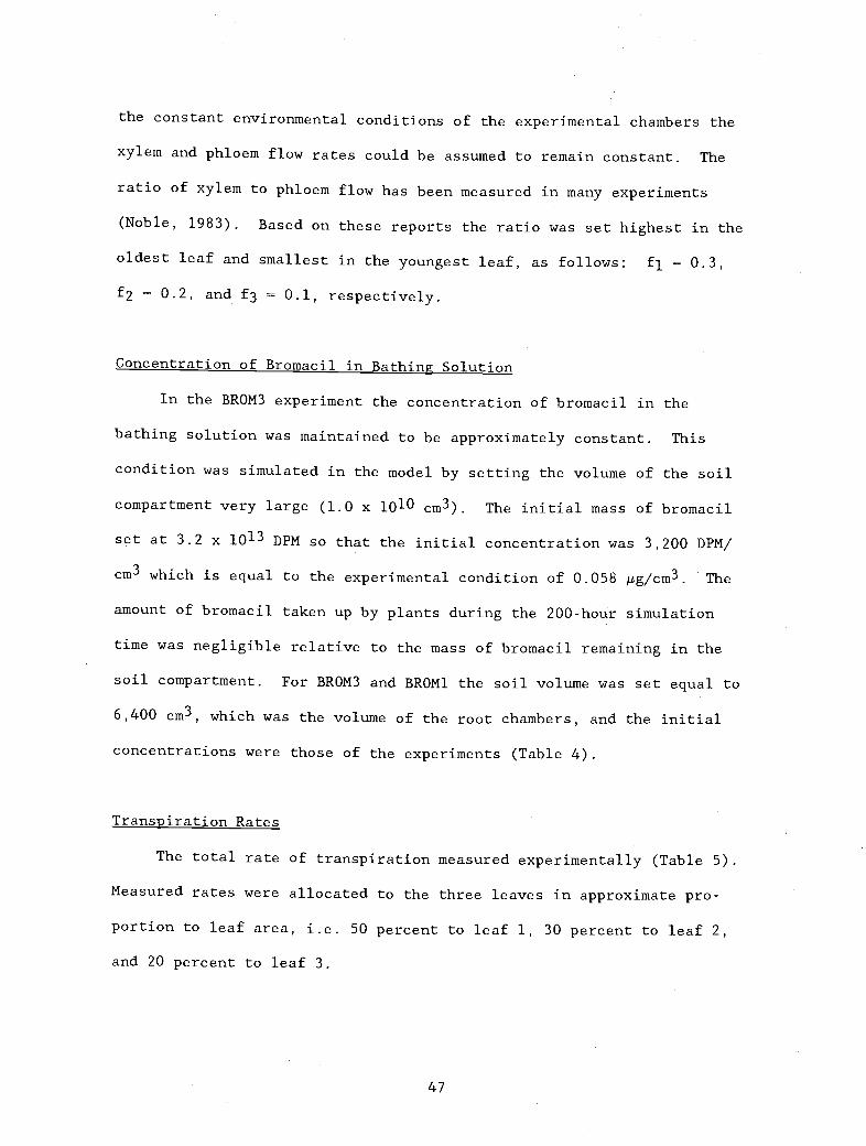
the constant environmental conditions of the experimental chambers the
xylem and phloem flow rates could be assumed to remain constant. The
ratio of xylem to phloem flow has been measured in many experiments
(Noble, 1983). Based on these reports the ratio was set highest in the
oldest leaf and smallest in the youngest leaf, as follows: = 0.3,
= 0.2, and f3 0.1, respectively.
Concentration of Bromacil in Bathing Solution
In the BROM3 experiment the concentration of bromacil in the
bathing solution was maintained to be approximately constant. This
condition was simulated in the model by setting the volume of the soil
compartment very large (1.0 x 1010 cm3). The initial mass of bromacil
set at 3.2 x 10¹³ DPM so that the initial concentration was 3,200 DPM/
cm3 which is equal to the experimental condition of 0.058 g/cm3. The
amount of bromacil taken up by plants during the 200-hour simulation
time was negligible relative to the mass of bromacil remaining in the
soil compartment. For BROM3 and BROM1 the soil volume was set equal to
6,400 cm3, which was the volume of the root chambers, and the initial
concentrations were those of the experiments (Table 4).
Transpiration Rates
The total rate of transpiration measured experimentally (Table 5).
Measured rates were allocated to the three leaves in approximate pro-
portion to leaf area, i.e. 50 percent to leaf 1, 30 percent to leaf 2,
and 20 percent to leaf 3.
47
THIS P
UBLICATIO
N IS O
UT OF D
ATE.
For mos
t curr
ent in
formati
on:
http:/
/exten
sion.o
regon
state.
edu/c
atalog

Storage Coefficients
The objective of the calibration procedure was to find plausible
values of the storage coefficients. Important qualitative observations
may be derived from Figures 3 through 5 and from literature reports.
The value of storage coefficients for molecules such as glycine may be
approximated from the relationship Q - (DKA/Ax) (equation 2 with a =
0). For such molecules D 0.036 cm2/hr. Assuming a = 0, Ax 0.1 cm,
and A = 1.0 cm2 obtains Q 0.360 cm3/hr for a surface area of 1 cm2.
There are many uncertainties with this estimate. The value for D is
for a dilute solution. Furthermore, only part of the surfaces of cells
are available for diffusion, making Q smaller than shown. Diffusion
may be limited by partitioning at the membrane surfaces. In the exper-
iments, the surface area of compartments could be much larger than
1 cm2. However, the value of Q = 0.360 cm3/hr provides a useful esti-
mate for the initial simulation.
In the leaves the rate of increase in bromacil concentration at
the medium-transpiration rate and low-exposure concentration (BROM5)
was approximately 0.100 x l0 DPM/g-hr (Figure 5). This corresponds to
(0.100 x l0) DPM/g-hr x (1.82 x l0) jig/DPM 1.82 x l0 pg/g-hr =
0.00182 pg/g-hr. This is the rate that would apply to 1 cm3 of storage
volume. For a storage volume of 10 cm3 the rate would be 0.0182 jig/hr.
The increase in concentration is the consequence of Qf and Qb thus
with Qb = 0.5 Qf the necessary Q should be 0.036 cm3/hr. Based on
these considerations, the initial guesses of Qf = 0.10 cm3/hr and Qb =
0.05 cm3/hr were used for stems and leaves.
Other considerations were that bromacil moves readily from trans-
port vessels to surrounding tissues as indicated by the rapid increase
48
THIS P
UBLICATIO
N IS O
UT OF D
ATE.
For mos
t curr
ent in
formati
on:
http:/
/exten
sion.o
regon
state.
edu/c
atalog

in concentrations in roots and stems following exposure. Storage
coefficients for phloem and xylem may therefore be assumed to be equal
to each other for a given tissue. Finally, we assumed that the storage
and mobilization coefficients are proportional to storage volume. This
proportionality derives from the volume to surface area relationship
indicated in equation 1.
49
THIS P
UBLICATIO
N IS O
UT OF D
ATE.
For mos
t curr
ent in
formati
on:
http:/
/exten
sion.o
regon
state.
edu/c
atalog
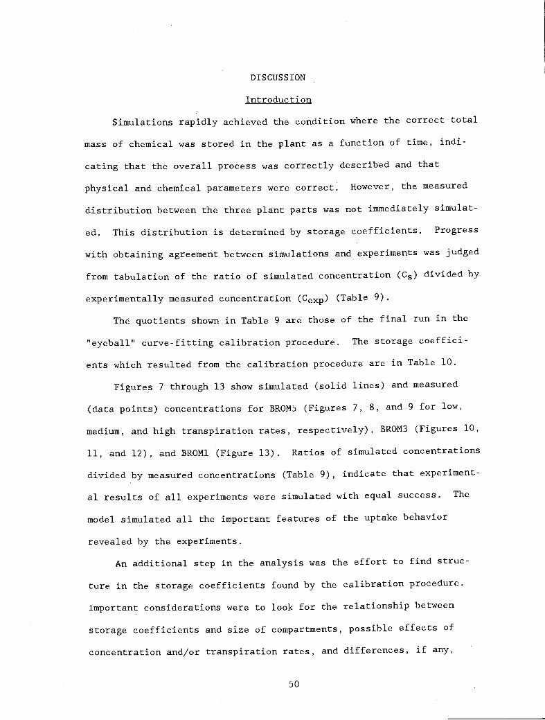
DISCUSSION
Introduction
Simulations rapidly achieved the condition where the correct total
mass of chemical was stored in the plant as a function of time, indi-
cating that the overall process was correctly described and that
physical and chemical parameters were correct. However, the measured
distribution between the three plant parts was not immediately simulat-
ed. This distribution is determined by storage coefficients. Progress
with obtaining agreement between simulations and experiments was judged
from tabulation of the ratio of simulated concentration (Cs) divided by
experimentally measured concentration (Cexp) (Table 9).
The quotients shown in Table 9 are those of the final run in the
"eyeball" curve-fitting calibration procedure. The storage coeffici-
ents which resulted from the calibration procedure are in Table 10.
Figures 7 through 13 show simulated (solid lines) and measured
(data points) concentrations for BROM5 (Figures 7, 8, and 9 for low,
medium, and high transpiration rates, respectively), BROM3 (Figures 10,
11, and 12), and BROM1 (Figure 13). Ratios of simulated concentrations
divided by measured concentrations (Table 9), indicate that experiment-
al results of all experiments were simulated with equal success. The
model simulated all the important features of the uptake behavior
revealed by the experiments.
An additional step in the analysis was the effort to find struc-
ture in the storage coefficients found by the calibration procedure.
Important considerations were to look for the relationship between
storage coefficients and size of compartments, possible effects of
concentration and/or transpiration rates, and differences, if any,
50
THIS P
UBLICATIO
N IS O
UT OF D
ATE.
For mos
t curr
ent in
formati
on:
http:/
/exten
sion.o
regon
state.
edu/c
atalog

E
a-0C0a
Ca)0C00
00
E
00C0a
-4-,
a)0C00
Brorn 5, LowTrans
Time (hrs)
Roots
Time (hrs)
Figure 7. Concentrations in roots, stems, and leaves as a function oftime for BROM5, low transpiration rate.
51
B5R 167
0
0
0
TTTTTTU0
000+
008
+
0 , ,i,i,,, ill iI liii , FT tlll4 111111111
g Brom 5, LowTrans Leaves B5.R I 67
Time (hrs)
Brom 5, LowTrans Sterna B5R 167
E
00C0aL.
Ca)0C00
THIS P
UBLICATIO
N IS O
UT OF D
ATE.
For mos
t curr
ent in
formati
on:
http:/
/exten
sion.o
regon
state.
edu/c
atalog

E
a-0C0.-0I.C4)000
E
0a£0
4-.0C4)0C00
30Time (hrs)
Figure 8. Concentrations in roots, stems, and leaves as a function of
time for BROM5, medium transpiration rate.
52
0
0
0
o Brom 5, MedTrans Leaves .varcioo00
0o00
0
TTT0, 4I
TTTTCD0r)
-
Time (hrs)
Brom 5, MedTrans Ste'n's B5R 168
Time (hrs)
Brom 5, MedTrans Roots B5R 168
THIS P
UBLICATIO
N IS O
UT OF D
ATE.
For mos
t curr
ent in
formati
on:
http:/
/exten
sion.o
regon
state.
edu/c
atalog
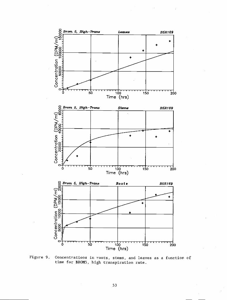
E
a_a-00c0
01._a
.1 0Co0C00 0
E
0.C
0aL..
C0C00
Brom 5, HighTrans
Brom0c: 5, HighTrans
53
Leaves
Time (hrs)
Stems
Time (hrs)
Figure 9. Concentrations in roots, stems, and leaves as a function oftime for BROM5, high transpiration rate.
+
B5R169
B5R 169
lull200
0
aL1I-
a+
++
a
aaa
+
aI)
aA
-,- .S- - -
5 .Urom b, HighTrans Roots B5.R169
+
+
+
Ari ur lilt T
11111111 1 I Ill I Ill I lilT! IT!0 50 100 150
Time (hrs)
C0a
a)C.)
00
THIS P
UBLICATIO
N IS O
UT OF D
ATE.
For mos
t curr
ent in
formati
on:
http:/
/exten
sion.o
regon
state.
edu/c
atalog

E
0aC0
.4-i0I.-
cwC.)
C00
0aC0a1.
Cq)000
54
, it. I I I) i ii r in rn rrrr. rrrT i ri rrrrr.
5
00U,
0 .- um-mni mm .
Brom 3, LowTrans Shoots B3R040
Brom 3, LowTrans Roots B3R040
0 10 20 30Time (hrs)
Figure 10. Concentrations in roots, stems, and leaves as a function oftime for BROM3, low transpiration rate.
0 10 20 30Time (hrs)
THIS P
UBLICATIO
N IS O
UT OF D
ATE.
For mos
t curr
ent in
formati
on:
http:/
/exten
sion.o
regon
state.
edu/c
atalog
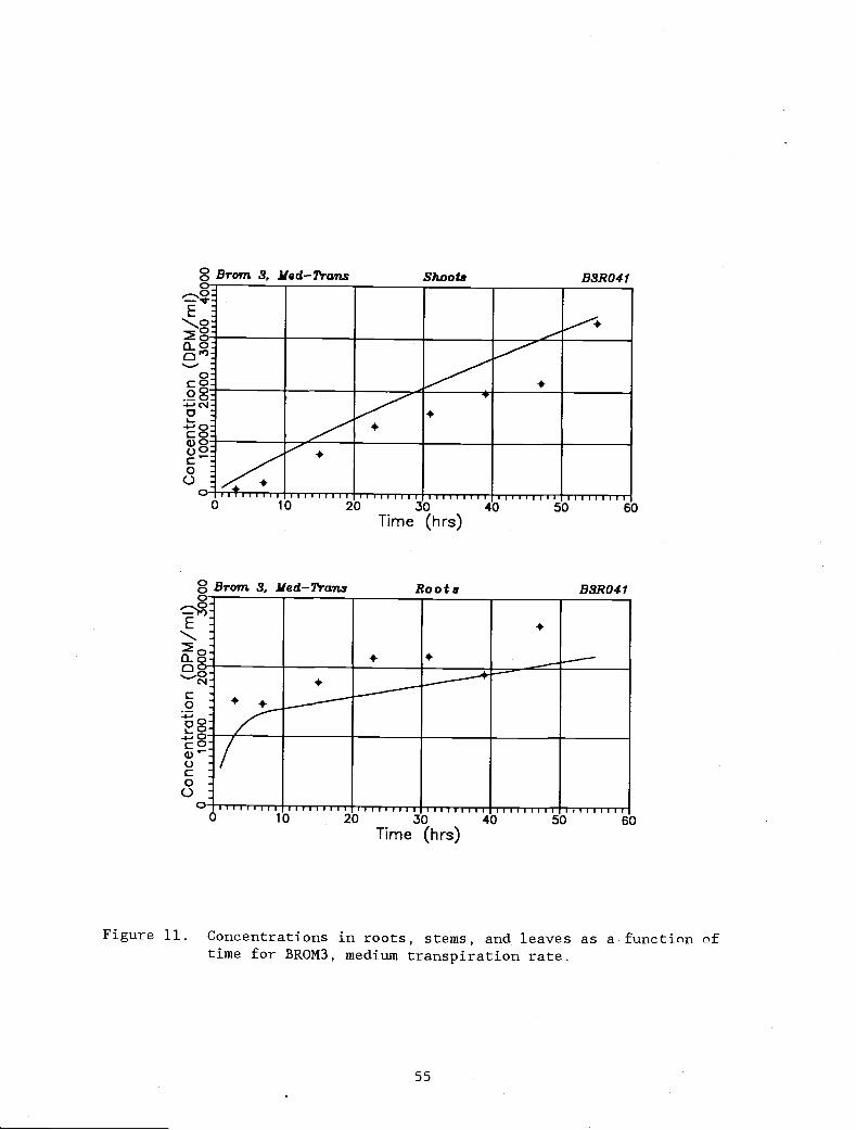
00
E
0'
.94-fla4-flCI
C00
E
a-
£0
I...
C)C00
Brom 3, MedTrans
55
Shoots B3.R04 I
60Time (hrs)
Figure 11. Concentrations in roots, stems, and leaves as a function oftime for BROM3, medium transpiration rate.
I 111 T 1U1 U1 I 11 I UUUI I
5 Urom S, MedTrans Roots)
B3.R041
41ll
)
JI.---
40 50 60Time (hrs)
THIS P
UBLICATIO
N IS O
UT OF D
ATE.
For mos
t curr
ent in
formati
on:
http:/
/exten
sion.o
regon
state.
edu/c
atalog
X Brom 3. HighTrans Shoots B3R042
0 10 20 30Time (hrs)
Figure 12. Concentrations in roots, stems, and leaves as a function of
time for BROM3, high transpiration rate.
56
oO
-+ +
+
+
) i-i-i-ri-I rTri ri, u-jr u i-u uVUET r i-ri-i
aU.)N0000N0 + +
+
+It) +
000000I')
o ii iliTil i__i liii, itT__Ti itli Iil ii TuTu!
0 10 20Time (hrs)
Brom 3. HiahTrans Roots B3R042
E
a-0
0.-I-a-1-iC'p()c00
E
a
0aC'p()C00
THIS P
UBLICATIO
N IS O
UT OF D
ATE.
For mos
t curr
ent in
formati
on:
http:/
/exten
sion.o
regon
state.
edu/c
atalog
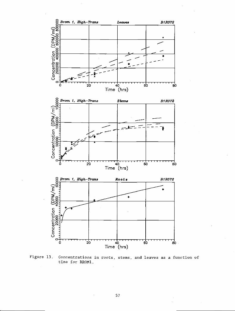
8 Brom 1,00
a-0Oco
00Co00zoa0Co
00Cc..l00
0
00 Brom I00
C0.-4-r 0-.- 0COQL)0C00
00
E
0aC00Ca)0C00
20 40Time (hrs)
57
B1R072
Figure 13. Concentrations in roots, stems, and leaves as a function oftime for BROM1.
£
-
- - - -
-
---4-------I
.-xA
$rom 1, HighTrans Roots B1R072
+
+
+
0 20 40 60 80
Time (hrs)
0 40 60 80
Time (hrs)
HighTrans Leavee B1R072
HighTrans Stems
6 80
THIS P
UBLICATIO
N IS O
UT OF D
ATE.
For mos
t curr
ent in
formati
on:
http:/
/exten
sion.o
regon
state.
edu/c
atalog
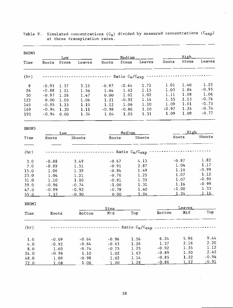
Table 9. Simulated concentrations (Cs) divided by measured concentrationsat three transpiration rates.
BROM5Low Medium High
Time Roots Stems Leaves Roots Stems Leaves Roots Stems Leaves
(hr) Ratio Cs/Cexp
8 -0.93 1.37 3.15 -0.97 -0.64 1.71 1.01 1.40 1.23
26 -0.88 1.21 1.54 1.04 1.62 1.15 1.03 1.84 -0.93
50 -0.97 1.26 1.47 0.00 1.01 1.02 1.11 1.08 1.06
122 0.00 1.05 1.06 1.21 -0.92 1.14 1.33 1.13 -0.76
145 -0.95 1.15 1.10 1.12 1.06 1.10 1.09 1.01 -0.73
169 -0.94 1.20 1.11 -0.98 -0.86 1.10 -0.97 1.26 -0.74
193 -0.94 0.00 1.34 1.04 1.05 1.31 1.09 1.09 -0.77
BROM3Low Medium High
Time Roots Shoots Roots Shoots Roots Shoots
BROM1Stem Leaves
Time Roots Bottom Mid Top Bottom Mid Top
(hr) Ratio Cs/Cexp
58
(Cexp)
(hr) Ratio Cs/Cexp
3.0 -0.88 3.49 -0.67 4.13 -0.87 1.82
7.0 -0.89 1.51 -0.91 2. 87 1.04 1.17
15.0 1.06 1.39 -0.84 1.49 1.10 -0.99
23.0 1.04 1.21 -0.76 1.25 1.07 1.12
31.0 1.10 1.10 -0.81 1.35 1.07 -0.90
39.0 -0.96 -0.74 -1.00 1.31 1.16 -0.99
47.0 -0.99 -0.92 -0.78 1.40 -1.00 1.33
55.0 1.27 -0.90 0.00 1.04 1.24 1. 16
1.0 -0.69 -0.64 -0.96 1.56 6 . 24 5.96 9 .44
4.0 -0. 92 -0.64 -0.63 1.26 1.37 2 . 16 2.20
8.0 1.03 -0.74 -0.75 1.25 -0.92 1.35 1.12
24.0 -0.96 1 . 10 1.02 1.63 -0.89 1.50 2.42
48 . 0 1 . 09 -0.98 1.02 1.14 -0.85 1.22 -0.94
72.0 1.08 1.06 1.20 1.28 -0.86 1.22 -0.91
THIS P
UBLICATIO
N IS O
UT OF D
ATE.
For mos
t curr
ent in
formati
on:
http:/
/exten
sion.o
regon
state.
edu/c
atalog

59
Table 10. Values of storage (forward) and mobilization (backward)transfer coefficient determined by the calibration procedureused in the text.
RatioCompartment Volume Q-f Q-b Qf/Qb
cm3 cni3/hr cm3/hrBROM5 - low
Root cortex 15.75 26.000 13.000 2.00.290 0.018 16.1
Root storage 5.743 0.190 0.009 21.1Stem bottom 3.076 0.405 0.050 8.1Stem middle 0.762 0.100 0.015 6.7Stem top 0.347 0.045 0.006 7.5Leaf bottom 8.183 0.104 0.013 8.0Leaf middle 4.910 0.070 0.009 7.8Leaf top 3.273 0.048 0.006 8.0
BROM5 -mediumRoot cortex 19.83 28.000 13.000 2.2
0.270 0.030 9.0Root storage 7.231 0.175 0.023 7.6Stem bottom 4.443 0.266 0.099 2.7Stem middle 1.100 0.068 0.027 2.5Stem top 0.502 0.030 0.012 1.5Leaf bottom 8.477 0.108 0.013 8.3Leaf middle 5.086 0.071 0.009 7.9Leaf top 3.391 0.049 0.006 8.2
BROM5 -high
Root cortex 20.08 31.000 13.000 2.40.200 0.038 5.3
Root storage 7.324 0.130 0.025 5.2Stem bottom 4.511 0.250 0.095 2.6Stem middle 1.117 0.065 0.0215 2.6Stem top 0.510 0.028 0.011 2.6Leaf bottom 9.751 0.118 0.015 7.9Leaf middle 5.851 0.0880 0.010 8.0Leaf top 3.900 0.055 0.007 7.9
BROM3 - low
Root cortex 29.01 25.000 13.000 1.90.375 0.031 12.1
Root storage 10.579 0.270 0.027 10.0Stem bottom 9.440 0.577 0.264 2.2Stem middle 2.338 0.146 0074 2.0Stem top 1.066 0.065 0.0 2.0Leaf bottom 28.155 0.217 0.027 8.0Leaf middle 16.893 0.168 0.021 8.0Leaf top 11.262 0.130 0.016 8.1
THIS P
UBLICATIO
N IS O
UT OF D
ATE.
For mos
t curr
ent in
formati
on:
http:/
/exten
sion.o
regon
state.
edu/c
atalog
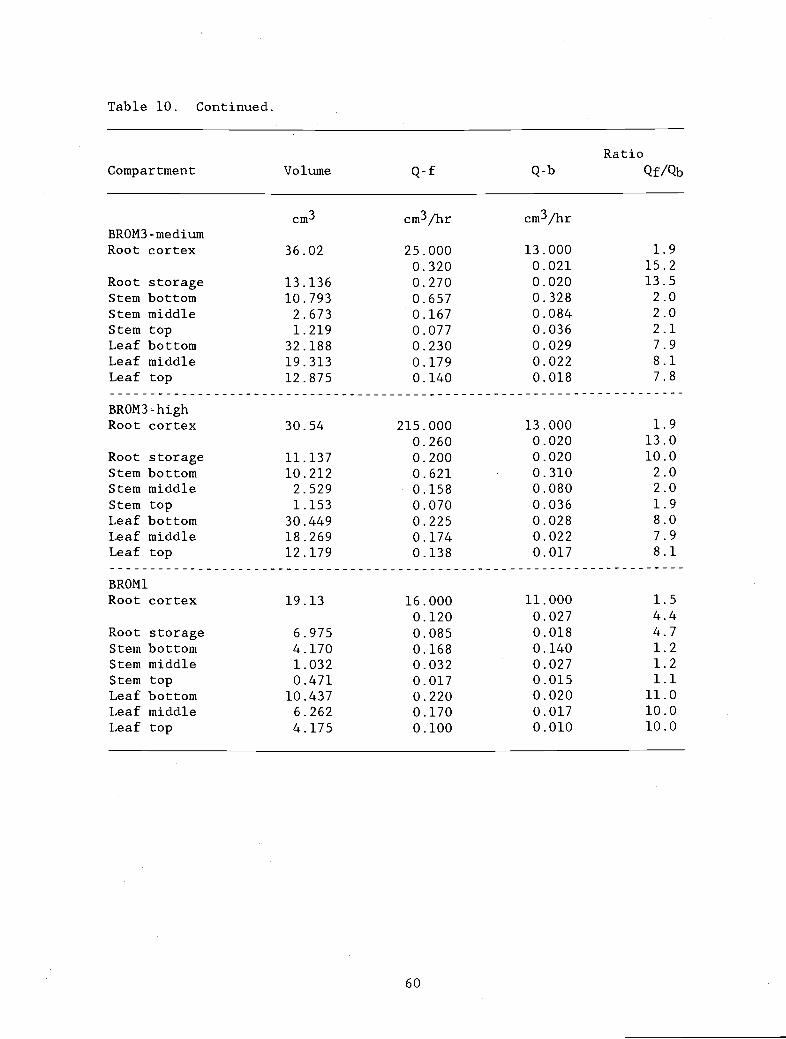
Table 10. Continued.
RatioCompartment Volume Q-f Q-b Qf/Qb
60
cm3 cm3/hr cm3/hrBROM3 -mediumRoot cortex 36.02 25.000 13.000 1.9
0.320 0.021 15.2
Root storage 13.136 0.270 0.020 13.5
Stem bottom 10.793 0.657 0.328 2.0
Stem middle 2.673 0.167 0.084 2.0
Stem top 1.219 0.077 0.036 2.1
Leaf bottom 32.188 0.230 0.029 7.9
Leaf middle 19.313 0.179 0.022 8.1
Leaf top 12.875 0.140 0.018 7.8
BROM3 -highRoot cortex 30.54 215.000 13.000 1.9
0.260 0.020 13.0
Root storage 11.137 0.200 0.020 10.0
Stem bottom 10.212 0.621 0.310 2.0
Stem middle 2.529 0.158 0.080 2.0
Stem top 1.153 0.070 0.036 1.9
Leaf bottom 30.449 0.225 0.028 8.0
Leaf middle 18.269 0.174 0.022 7.9
Leaf top 12.179 0.138 0.017 8.1
BROM1Root cortex 19.13 16.000 11.000 1.5
0.120 0.027 4.4
Root storage 6.975 0.085 0.018 4.7
Stem bottom 4.170 0.168 0.140 1.2
Stem middle 1.032 0.032 0.027 1.2
Stem top 0.471 0.017 0.015 1.1
Leaf bottom 10.437 0.220 0.020 11.0
Leaf middle 6.262 0.170 0.017 10.0
Leaf top 4.175 0.100 0.010 10.0
THIS P
UBLICATIO
N IS O
UT OF D
ATE.
For mos
t curr
ent in
formati
on:
http:/
/exten
sion.o
regon
state.
edu/c
atalog

between the three plant parts. To prepare for this analysis the ratios
Qf/Qb shown in Table 10 were reordered as shown in Table 11.
Roots
Root concentrations increased rapidly during the first hours of
exposure (Figures 7 through 13). The duration of this period of rapid
uptake decreased with increasing concentration of the bathing solution.
This uptake pattern was reproduced by the model by using large storage
coefficients during this initial period. The large storage coeffi-
cients were changed to lower values after 10 hours of simulation for
BROM5, 8 hours for BROM3, and 6 hours for BROM1. The uptake behavior
reflected the rapid uptake which occurred upon the initial entry of
solution into the root-free space. The medium transpiration rate for
BROM5 was 5.7 cm3/hr per plant; the root volume was 23.3 cm3, consist-
ing of 3.5 cm3 apparent free space and 19.8 cm3 cortex volume. At the
indicated transpiration rate, the water in the 3.5 cm3 of apparent free
space would be flushed out in 0.6 hour. Uptake after that time repre-
sents rapid storage in the cortex cells.
The instantaneous exposure would not occur under field conditions,
except where a spill of contaminant occurred so that contaminated water
would reach the root zone over a short period of time. For such condi-
tions, the model should be run as done here. More likely is the
scenario with low-level, chronic exposure such as occurs where plants
are growing in contaminant soil water. The chronic exposure should be
modeled using the smaller storage coefficients. Following the rapid
initial uptake, storage continued in the root cortex and storage com-
partment of the root stele at a lower rate.
61
THIS P
UBLICATIO
N IS O
UT OF D
ATE.
For mos
t curr
ent in
formati
on:
http:/
/exten
sion.o
regon
state.
edu/c
atalog
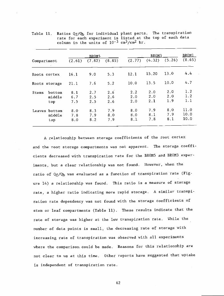
Table 11. Ratios Qf/Q13 for individual plant parts. The transpirationrate for each experiment is listed at the top of each data
column in the units of iO-3 cm3/cm2 hr.
A relationship between storage coefficients of the root cortex
and the root storage compartments was not apparent. The storage coeffi-
cients decreased with transpiration rate for the BROM5 and BROM3 exper-
iments, but a clear relationship was not found. However, when the
ratio of Qf/Qb was evaluated as a function of transpiration rate (Fig-
ure 14) a relationship was found. This ratio is a measure of storage
rate, a higher ratio indicating more rapid storage. A similar transpi-
ration rate dependency was not found with the storage coefficients of
stem or leaf compartments (Table 11). These results indicate that the
rate of storage was higher at the low transpiration rate. While the
number of data points is small, the decreasing rate of storage with
increasing rate of transpiration was observed with all experiments
where the comparison could be made. Reasons for this relationship are
not clear to us at this time. Other reports have suggested that uptake
is independent of transpiration rate.
62
CompartmentBROM5 BROM3 BROM1
(2.61) (7.82) (8.85) (2.77) (4.32) (5.26) (8.65)
Roots cortex 16.1 9.0 5.3 12.1 15.20 13.0 4.4
Roots storage 21.1 7.6 5.2 10.0 13.5 10.0 4.7
Stems bottom 8.1 2.7 2.6 2.2 2.0 2.0 1.2
middle 6.7 2.5 2.6 2.0 2.0 2.0 1.2
top 7.5 2.5 2.6 2.0 2.1 1.9 1.1
Leaves bottom 8.0 8.3 7.9 8.0 7.9 8.0 11.0
middle 7.8 7.9 8.0 8.0 8.1 7.9 10.0
top 8.0 8.2 7.9 8.1 7.8 8.1 10.0
THIS P
UBLICATIO
N IS O
UT OF D
ATE.
For mos
t curr
ent in
formati
on:
http:/
/exten
sion.o
regon
state.
edu/c
atalog

63
I I I
0 2 4 6 8 10
Transpiration Rate (cm3 I cm2! hr)
Figure 14. Ratio Qf/Qb for the root cortex and for root storage com-partments as a function of transpiration rate.
THIS P
UBLICATIO
N IS O
UT OF D
ATE.
For mos
t curr
ent in
formati
on:
http:/
/exten
sion.o
regon
state.
edu/c
atalog

Stems
The relationship between storage coefficients and stem volumes was
found to be linear (Figure 15). The same relationship applied to all
experiments except BROM5, low transpiration rate. The proportionality
in the absence of a transpiration or concentration effect reflects the
proportionality of storage with surface area, as was previously dis-
cussed.
Leaves
Storage coefficients of leaves were related to leaf volume in an
exponential manner (Figure 16). The relationship was the same for
BROM5 and BROM3 experiments, but had a higher exponent for the BROM1
experiment. The difference between the BROM1 and the other two experi-
ments may indicate a concentration effect. Storage coefficients did
not increase with the increase of concentration from BROM5 to BROM3,
but increased about 50 percent by increasing the concentration from
BROM3 to BROM1. This concentration effect may result from an affect of
bromacil on plant tissue which occurs at the much higher concentrations
in the leaf with the BROM1 experiment. This effect was also shown
earlier in Figure 6.
64
THIS P
UBLICATIO
N IS O
UT OF D
ATE.
For mos
t curr
ent in
formati
on:
http:/
/exten
sion.o
regon
state.
edu/c
atalog
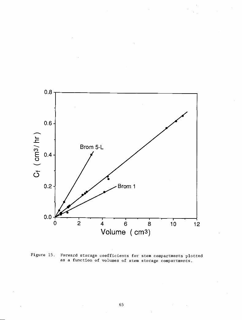
0
2-I -. 1
4 6 8 10
Vo'ume (cm3)
Figure 15. Forward storage coefficients for stem compartments plottedas a function of volumes of stem storage compartments.
65
12
THIS P
UBLICATIO
N IS O
UT OF D
ATE.
For mos
t curr
ent in
formati
on:
http:/
/exten
sion.o
regon
state.
edu/c
atalog

0.25
0.20-
0.05-
0.00! I I F
0 5 10 15
Volume
66
I I
20 25
(cm3)30 35
Figure 16. Forward storage coefficients for leaf compartments plotted
as a function of volumes of leaf storage compartments.
THIS P
UBLICATIO
N IS O
UT OF D
ATE.
For mos
t curr
ent in
formati
on:
http:/
/exten
sion.o
regon
state.
edu/c
atalog

SENSITIVITY ANALYSIS
Introduction
One of the best methods for choosing the parameters in a sensitiv-
ity study of a mathematical model is the factorial design (Box et al.,
1978). This "experimental design" is practical when the number of
independent parameters is less than or equal to 10. However, UTAB 4.6
contains more than 200 independent parameters. It is therefore not
practical to choose a factorial design for varying the parameters. It
is also nearly impossible to set up and solve, in closed form, a set of
sensitivity equations as described by Bard (1974). For purposes of
this report only some of the individual parameters which are important
to the uptake, accumulation, and translocation processes were varied.
The results of changing these parameters are compared with BROM5 medium
transpiration rate as the reference simulation. Nineteen sets of
simulations were made. The parameters which were evaluated and their
values are in Table 12. Results are shown in Figures 17 through 27.
Transpiration Rate
The transpiration rate used for the reference simulation was that
of the BROM5 medium transpiration rate (Table 12). The curves labeled
Ref in Figure 17 correspond to this transpiration value. The curve
labeled A corresponds to the simulation with the low transpiration
rate, while the curve labeled B corresponds to the simulation with the
high transpiration rate. Simulations show an increase in concentration
in all three plant parts as a result of increasing the transpiration
rate and a decrease in all three plant parts as a result of decreasing
the transpiration rates. On a relative basis, the effect of increasing
67
THIS P
UBLICATIO
N IS O
UT OF D
ATE.
For mos
t curr
ent in
formati
on:
http:/
/exten
sion.o
regon
state.
edu/c
atalog
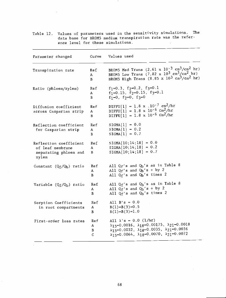
Table 12. Values of parameters used in the sensitivity simulations. The
data base for BROM5 medium transpiration rate was the refer-
ence level for these simulations.
Parameter changed Curve Values used
Transpiration rate Ref BROM5 Med Trans (2.61 x l0 cm3/cm2 hr)
A BROM5 Low Trans (7.82 x lO cm3/cm2 hr)
B BROM5 High Trans (8.85 x iO3 cm3/cm2 hr)
Ratio (phloem/xylem) Ref f1=0.3, f2=0.2, f30.lA f1=O.15, f2=O.15, f3=O.lB f1=0, f2=0, f3=0
Diffusion coefficient Ref DIFFU[1] = 1.8 x .i0 cm2/hr
across Casparian strip A DIFFU[1] = 1.8 x 10⁻⁶ Gm2/hrB DIFFU[1J = 1.8 x 10⁻⁶ Gm2/hr
Reflection coefficient Ref SIGMA[l} 0.0
for Casparian strip A SIGMA{1] = 0.2
B SIGMA[1} = 0.7
Reflection coefficient Ref SICMA[1O;l4;181 = 0.0
of leaf membrane A sICMA{lO;14;18] = 0.2
separating phloem and B SIGMA[l0;l4;l81 = 0.7
xylem
Constant (Qf/Qb) ratio Ref All Qf's and Qb's as in Table 8
A All Qf's and Qb's by 2
B All Qf's and Qb' times 2
Variable (Qf/Qb) ratio Ref All Qf's and Qb' as in Table 8
A All Qf's and Qb's by 2
B All Qf's and Qb' times 2
Sorption Coefficients Ref All B's = 0.0
in root compartments A B(l)=B(3)=0.5B B(l)=B(3)=l.0
First-order loss rates Ref All )'s 0.0 (l/hr)
A A15=0.0016, l80.00175, X2l=0.00l8B A15=0.0032, Al8=0.0035, .X21=0.0036C .XlS=0.0064, .X18=0.0070, A21=0.0072
68
THIS P
UBLICATIO
N IS O
UT OF D
ATE.
For mos
t curr
ent in
formati
on:
http:/
/exten
sion.o
regon
state.
edu/c
atalog
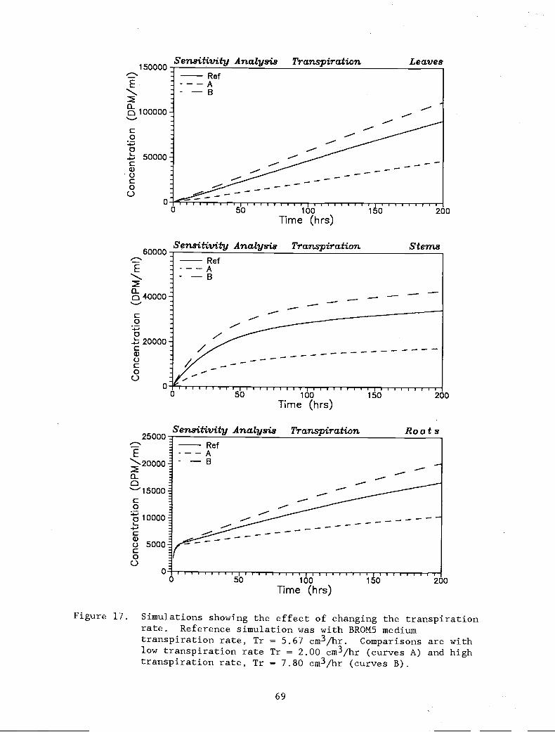
£00
-4-,
a)000
150000Sensitivity Analysis
E
100000
50000
0
60000
E
40000
Co
-4-,020000 =
£a)0C00
25000
Ref---A- B
--
- -
0
E-20O00 -
a-a'"15000Co
11000015000
000
0
Sensitivity Analysis Trans-pirationRefAB
/ V
I r I I I L I I I I I -1 I50 100
Time (hrs)
5b
50 100Time (hrs)
Sensitivity Analysis TranspirationRef--AB
69
Transpiration
id I rI
150
Leaves
Stems
Roots
200
Figure 17. Simulations showing the effect of changing the transpirationrate. Reference simulation was with BROM5 mediumtranspiration rate, Tr = 5.67 cm3/hr. Comparisons are withlow transpiration rate Tr = 2.00 cm3/hr (curves A) and hightranspiration rate, Tr = 7.80 cm3/hr (curves B).
200I- I I I -E I I I-
100Time (hrs)
THIS P
UBLICATIO
N IS O
UT OF D
ATE.
For mos
t curr
ent in
formati
on:
http:/
/exten
sion.o
regon
state.
edu/c
atalog

the transpiration rate was much smaller than the effect of decreasIng
the transpiration rate. The decrease in the transpiration rate by 67
percent decreased the concentration at 200 hours in the leaves
(curve A) from 1.57 x 10⁶ to 8.09 x lO dpm/gm, in the stems from
2.23 x lO to 1.14 x lO dpm/gm, and in the roots from 5.21 x lO to
3.26 x i05 dpm/gm. On the other hand, increasing the transpiration
rate by 13 percent (curve B) produced a corresponding increase in the
concentrations of the three plant regions. The increases in concentra-
tions were from 1.57 x 10⁶ to 1.93 x 10⁶ dpm/g in the leaves, from
2.23 x l0 to 2.78 x lO dpni/g in the stems, and from 5.21 x lO to
6.31 x l0 dpm/g in the roots. These simulations show that the effects
of increasing transpiration rates are not linear. The increase in
concentrations diminishes as concentrations become higher.
Ratio: Phloem Transport RatLXylem Transport Rate
The ratio (phloem transport rate/xylem transport rate) is a mea-
sure of the mobility of the chemical in the plant. A higher ratio
means that chemical accumulating in the leaves readily enters the
phloem pathway through which it is transported back to the roots. The
expectation is that a low ratio increases the concentrations in the
leaves and decrease concentrations in stems and roots, whereas a high
ratio decreases the concentrations in the leaves and increases concen-
trations in stems and roots. Results agreed with these expectations
(Figure 18). Simulation with the ratios equal to zero (curve A), i.e.
no phloem transport, showed the expected increase in concentrations in
the leaves and decrease in stems and roots. The decrease in concentra-
tions in stems and roots were large, namely from 2.23 x i05 to 5.12 x
70
THIS P
UBLICATIO
N IS O
UT OF D
ATE.
For mos
t curr
ent in
formati
on:
http:/
/exten
sion.o
regon
state.
edu/c
atalog
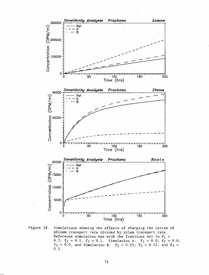
E
co0CC,0C00
40000
E
-C -
c 20000
j
20000
E
15000:C
I5000:
0-'0
Sensitivity Analysis Fractions- Ref--AB/
-
Sensitivity Analysis
71
I 1 1 1I 1 I I I I I
50 100Time (hrs)
-
Fractions
I I 1U 1
50 100Time (hrs)
Stems
Root.s
200
200
Figure 18. Simulations showing the effects of changing the ratios ofphloem transport rate divided by xylem transport rate.Reference simulation was with the fractions set to f1 =0.3; f2 = 0.2, f3 0.1. Simulation A: f1 0.0; f2 = 0.0,f3 = 0.0, and Simulation B: f1 = 0.15; f2 = 0.15, and f3 =0.1.
Sert.sdivtiy Analysis300000
Fractions LeavesRefAB
200000
ioo000
50 100Time (hrs)
150 200
THIS P
UBLICATIO
N IS O
UT OF D
ATE.
For mos
t curr
ent in
formati
on:
http:/
/exten
sion.o
regon
state.
edu/c
atalog

iO4 dpm/g in the stems and from 5.21 x i05 to 2.63 x iO dpm/g in the
roots. The increase in the leaves was dramatic, namely from 1.57 x 10⁶
to 3.52 x 10⁶ dpm/g. Simulation with the phloem/xylem ratio greater
than zero showed the expected increase in the stems, namely from 2.23 x
lO to 2.52 x lO dpm/g, but there was no change in the concentrations
in the roots when compared with the reference simulation. Concentra-
tion in the leaves were lowest with the reference simulation. The fact
that for ratios greater than 0.1 the concentration in the roots did not
respond to the further increases indicates that this process is no
longer a rate-limiting process. Compound is being recycled sufficient-
ly fast so that storage is the rate-limiting process. The small in-
crease in concentrations in the leaves relative to the reference curve,
namely from 1.57 x 10⁶ to 1.89 x 10⁶ dpm/g, is attributed to the fact
that the slower recycling results in a longer residence time in the
leaves which thereby increases the leaf storage of bromacil.
Diffusion Coefficient of the Casparian Strip
For this simulation the diffusion coefficient of the Casparian
strip was changed. This coefficient determines the rate at which
diffusion across the Casparian strip can occur. The value of this
coefficient is important with respect to diffusion from the root xylem
and phloem compartments back to the root cortex. The role played by
this coefficient can be learned from the mass balance equations, spe-
cifically equations (9) and (21). The expectation was that a decrease
in the diffusion coefficient would increase the amount of chemical in
the plant and therefore increase the concentrations in all compart-
ments. Similarly, an increase in the diffusion coefficient at the
72
THIS P
UBLICATIO
N IS O
UT OF D
ATE.
For mos
t curr
ent in
formati
on:
http:/
/exten
sion.o
regon
state.
edu/c
atalog

Casparian strip was expected to decrease the total amount of chemical
in the plant and therefore produce a decrease in the concentrations in
all plant compartments. These expectations were borne out by the
simulations shown in Figure 19. The effects were not linear, however.
The effect of increasing the diffusion coefficient by a factor of 10
was somewhat larger than that of decreasing it by the same factor.
Increasing the coefficient decreased the concentrations at 200 hours in
the leaves from 1.57 x 10⁶ to 1.18 x 10⁶ dpm/gm, in the stems from
2.23 x i05 to 1.60 x lO dpm/gm, and in the roots from 5.21 x lO to
4.25 x lO dpm/gm. Increasing the diffusion coefficient increased the
concentrations in the leaves from 1.57 x 10⁶ to 2.33 x 10⁶ dpm/gm, in
the stems from 2.23 x l0 to 3.54 x l0 dpm/gm, and in the roots from
5.21 x l0 to 7.07 x l0 dpm/gm.
Reflection Coefficient of the Casparian Strii
The reflection coefficient is a measure of the ease of passing
across the Casparian strip. A reflection coefficient equal to zero
allows the chemical to pass unimpeded, a reflection coefficient equal
to one does not allow any chemical to pass this barrier. All plant
parts were expected to be influenced equally by changes in the reflec-
tion coefficient of the Casparian strip. This expectation was con-
firmed by the results (Figure 20). With the reflection coefficient
equal to 0.2, concentrations in leaves decreased from 1.57 x 10⁶ to
1.42 x 10⁶ dpm/gm, in the stems from 2.23 x l0 to 2.01 x l0 dpm/gm,
and in the roots from 5.21 x to 4.83 x l0 dpm/gm. Setting the
reflection equal to 0,7'further decreased concentrations, namely from
1.57 x 10⁶ to 1.03 x 10⁶ dpm/grn in the leaves, from 2.23 x l0 to
73
THIS P
UBLICATIO
N IS O
UT OF D
ATE.
For mos
t curr
ent in
formati
on:
http:/
/exten
sion.o
regon
state.
edu/c
atalog
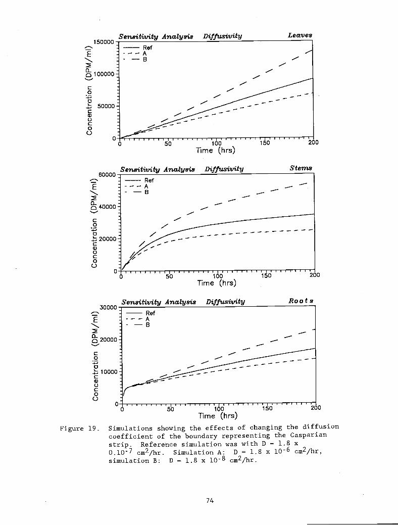
Sens*vity Analysis150000
E
100000
C0o =I-
000
E
4-0000 -
C00
0C00
Sen.sitivitj Analysis Diffusivity60000
30000
00
E
20000 -
0
I-C
0c00
RefAB
Ref--AB
lip''50
5'O
1 1 I I r p r r I100
Time (hrs)
74
T 1 I I r I- I I T
100Time (hrs)
Sensitivity Analysis Diffusiv'ity
-
'id
II150
-
I.) T I I I I- T I r I- I I I I I I J
0 50 100 150Time (hrs)
Figure 19. Simulations showing the effects of changingcoefficient of the boundary representing thestrip. Reference simulation was with D = 1.0.l0- cm2/hr. Simulation A: D = 1.8 x 10simulation B: D = 1.8 x 10⁻⁸ cm2/hr.
200
Stems
Roots
200
200
the diffusionC as par ian
8x6 cm2/hr,
LeavesDiffusivity
THIS P
UBLICATIO
N IS O
UT OF D
ATE.
For mos
t curr
ent in
formati
on:
http:/
/exten
sion.o
regon
state.
edu/c
atalog

80000 -
40000 -
0
40000
E
30000 -a-0
20000
10000.o =C -0 -o
20000
E
15000a-a
10000
50000C00
0
0
Sensitivity
0
5'O
Analysis Sigma, CpSt
till 1111150
-r i i-i100
Time (hrs)
Sensitivity Analysis Sigma, CpSt
I I I r I I I 1 I p
100 150Time (hrs)
Time (hrs)
Figure 20. Simulation showing effects of changing the reflectioncoefficient of the boundary representing the Casparianstrip. Reference simulation was with a = 0.0.
Simulation A: a = 0.2; simulation B: a = 0.7.
75
Stems
200
I I ll I200
Roots
Sensitivity Analysis Sigma.1, CpSt Leaves120000
THIS P
UBLICATIO
N IS O
UT OF D
ATE.
For mos
t curr
ent in
formati
on:
http:/
/exten
sion.o
regon
state.
edu/c
atalog
1.46 x dpm/gm in the stems, and from 5.21 x i05 to 3.91 x
i05 dpm/gm in the roots.
Reflection Coefficients in the Leaf Membranes Separating Xylem and
Phloem Pathway
The reflection coefficient of the membrane separating xylem and
phloem pathways is a measure of the ease with which the chemical can
enter the phloem pathway. An increase in this reflection coefficient
in the leaves was expected to increase concentrations in the leaf
despite the "choking-off" effect an increasing a has. The concentra-
tions in the leaf xylem increased under these conditions, thereby driv-
ing more compound into storage. Concentration in stems and roots were
expected to decrease as the entry into the phloem system was decreased
by the increasing reflection coefficients. These expectations were
confirmed by the simulations. Figure 21 shows that concentrations
increased in the leaves and decreased in stems and roots. Changes from
the reference level with the reflection coefficient equal to zero to
the simulation with a = 0.2 were small. A larger change occurred with
the reflection coefficient a = 0.7. With these simulations the total
amount of chemical in the plant was the same so that increases in leaf
concentrations corresponded to decreases in stem and root concentra-
tions.
Storage Coefficients
The role played by the storage and mobilization coefficients was
discussed in detail in the text of this report. The values of the
storage coefficients, Qf's, and the mobilization coefficients, Qb's,
76
THIS P
UBLICATIO
N IS O
UT OF D
ATE.
For mos
t curr
ent in
formati
on:
http:/
/exten
sion.o
regon
state.
edu/c
atalog

150000Sensitivtty Analysis Sigma, Leaf
E
l00000
C00
- 50000-Cq)0C00
E
30000 -o
20000
I
00
Sens'tivity Analys'ts Sigma, Leaf40000
0
RefA- B
/ V
501 1 I 16r I I T
Time (hrs)
111111 I I r' r- IIIIJIU50 100
Time (hrs)
r Tillil ri IIlJ0 50 100 150 200
Time (hrs)
Figure 21. Simulations showing the effects of changing the reflectioncoefficients of the membranes in the leaves which separatephloem from xylem (alO, al4, and al8). Reference simulation
was with the three coefficients equal to zero. Simulation A,
a's equal to 0.2; Simulation B, a's equal to 0.7.
I'
77
Leaves
Stems
I 11111200
200
20000Semsi.tivity Analysis Sigma, Leaf Roots
E
15000-0
10000-
5000-
THIS P
UBLICATIO
N IS O
UT OF D
ATE.
For mos
t curr
ent in
formati
on:
http:/
/exten
sion.o
regon
state.
edu/c
atalog
were increased by a factor of 2 (curves B) in one simulation and de-
creased by a factor of 2 (curves A) in the second simulation. With
these changes the ratios Qf/Qb remained the same. Figure 22 shows that
the simultaneous increase of Qf's and Qb' by a factor of 2 increased
the concentrations in leaves, while decreasing concentrations in the
stems and increasing concentrations in the roots. The increases in the
leaves was from 1.57 x 10⁶ to 2.07 x 10⁶ dpm/gm, the decrease in the
stems was from 2.23 x lO to 1.94 x lO dpm/gm, and the increase in the
roots was from 5.21 x lO to 5.45 x lO dpm/gm. The ratio (Qf/Qb) of
the leaves was higher than for the other two plant parts, so that an
increase by a factor of 2 resulted in increased storage. Since more of
the chemical taken up by the plant was stored in the leaves, less
remained available for storage in stems and roots. In the competition
for chemical to be stored, the stems were the most strongly effected,
with little change in the roots.
When values of (Qf/Qb) were decreased by a factor of 2, uptake in
the leaf decreased, as did the uptake in the roots; however, uptake by
the stems increased. The simulation resulted in a lower concentrations
in the leaves, as expected. Reasons for the increases in stems and
decreases in roots are not clear. Since the ratios were not changed
the final concentrations at very long time values are the same for all
simulations. However, the rate at which equilibrium concentrations are
achieved depends on the ratio (Qf/Qb).
78
THIS P
UBLICATIO
N IS O
UT OF D
ATE.
For mos
t curr
ent in
formati
on:
http:/
/exten
sion.o
regon
state.
edu/c
atalog
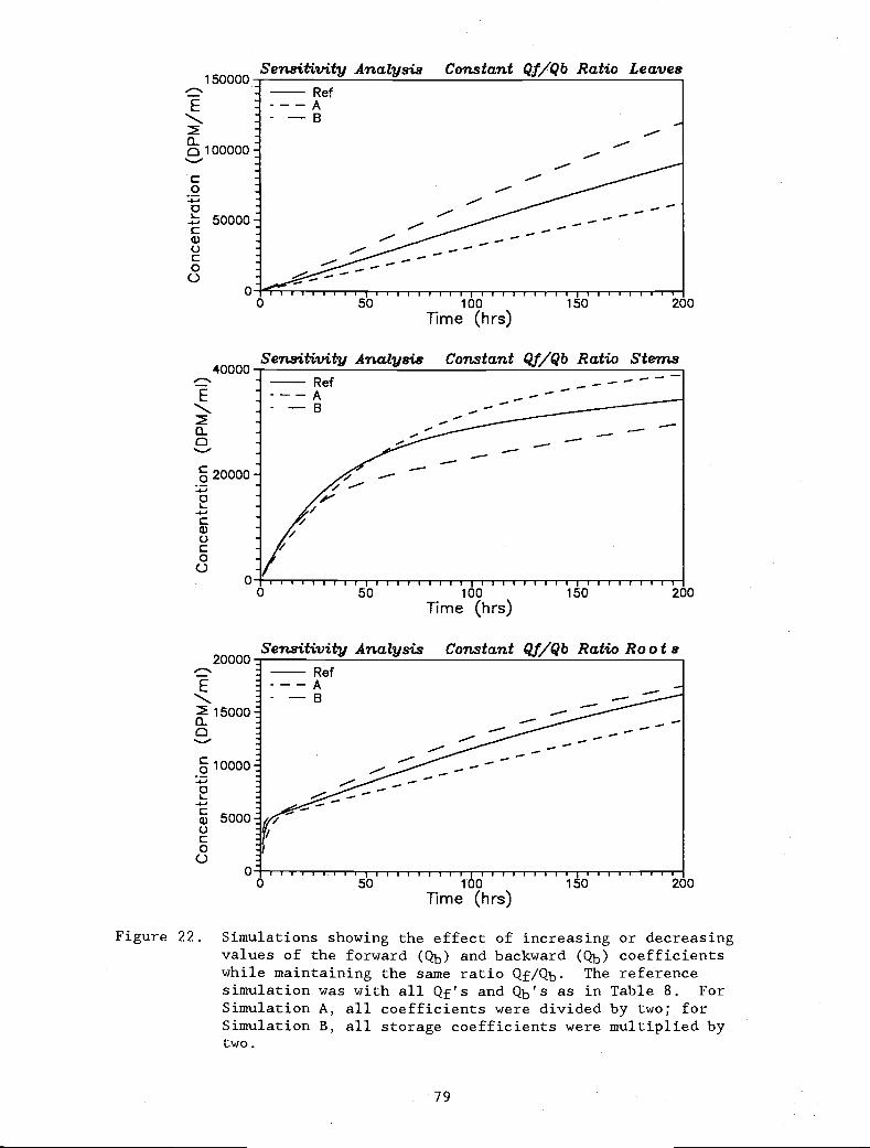
E
00I-
-4-,C1)()C00
40000
E
-0 -
c 20000 -
20000
E
1500000
110000_5000-
I I -I
50
0 ,, ,,,.i,-,,. II0 50
Sensitivity Analysis
I I I- I I- I I I I I I100 150
Time (hrs)
Constant Qf/Qb Ratio Roots
200
UT IUU I100
Time (hrs)
Figure 22. Simulations showing the effect of increasingvalues of the forward (Qb) and backward (Qb)while maintaining the same ratio Qf/Qb. Thesimulation was with all Qf's and Qb's as inSimulation A, all coefficients were dividedSimulation B, all storage coefficients weretwo.
79
200
or decreasingcoefficientsreference
Table 8. Forby two; formultiplied by
Sensttivtty Analysi.s Constant Qf/Qb Ratio Leaves
0 5'O i6o 200Time (hrs)
StemsSensttivity Analysis Constant Qf/Qb Ratio
THIS P
UBLICATIO
N IS O
UT OF D
ATE.
For mos
t curr
ent in
formati
on:
http:/
/exten
sion.o
regon
state.
edu/c
atalog

Change in the Ratio Q,/Qh
When the ratio Qf/Qb was changed, equilibrium concentrations, as
well as rates of approach to equilibrium, changed in each plant part.
With the ratio increased by a factor of 2 (curves B), storage increased
and the increases were similar for all three plant parts. Figure 23
shows that the increases were from 1.57 x 10⁶ to 2.18 x 10⁶ dpm/gm for
leaves, from 2.23 x lO to 1.00 x lO dpm/gm for stems, and from 5.21 x
l0 to 7.78 x l0 dpm/gm for roots. Concentrations decreased in all
plant parts by decreasing the Qf/Qb (curves A) ratios, and the
decreases were about the same for each plant part. The decreases were
from 1.57 x 10⁶ to 1.00 x 10⁶ dpm/gm for leaves, from 2.23 x lO to
1.46 x i05 dpm/gm for stems, and from 5.21 x l0 to 3.28 x i05 dpm/gm
for roots.
Sorption Coefficients in the Root Stora.ge Compartments
The sorption coefficients allow linear equilibrium sorption to
occur. The effect is equivalent to that of increasing the volume of a
compartment in which sorption occurs. Figure 24 shows simulations with
the sorption coefficients of the root storage compartments set equal to
0.5 and 1.0. Results (Figure 24) indicate that these changes did not
change the concentrations of the leaves and stems, but concentrations
in the root compartments increased, as was expected. The increase was
from 5.21 x l0 to 6.47 x l0 dpm/gm for B1 = B3 = 0.5, and from 5.21 x
l0 to 7.50 x l0 dpm/gm for B1 = B3 = 1.0.
80
THIS P
UBLICATIO
N IS O
UT OF D
ATE.
For mos
t curr
ent in
formati
on:
http:/
/exten
sion.o
regon
state.
edu/c
atalog

E
100000 -
C00
- 50000-ca)()C00
0
60000
30000
E
20000
00Cci
0C00
0
E
40000
C0
.e-0
20000 -Ca)0C00
Sensitivity Analysis Variable Qf/Qb Ratio StemsRef--AB
111111 11111 III tiiiij liii50 100 150
Time (hrs)
Sensitivity Analysis Variable Qf/Qb Ratio Ro o t s
I
RefA- B
200
Figure 23 Simulations showing the effects of changing the ratios offorward storage coefficients to the backward storage coeff i-cients. Reference simulation was with all storage coefficients as shown in Table 8. For Simulation A, all forwardstorage coefficients (Q) were divided by two while leavrthe Qb the same; for Simulation B, all forward storagecoefficients were multiplied by two, while leaving the Qb'sthe same.
81
Sensitivity Analysis Variable Qf/Qb Ratio Leaves150000
200-I
100Time (hrs)
5b0
I,,,, rJiJ till VT liiiI
150 2000 50 100Time (hrs)
THIS P
UBLICATIO
N IS O
UT OF D
ATE.
For mos
t curr
ent in
formati
on:
http:/
/exten
sion.o
regon
state.
edu/c
atalog
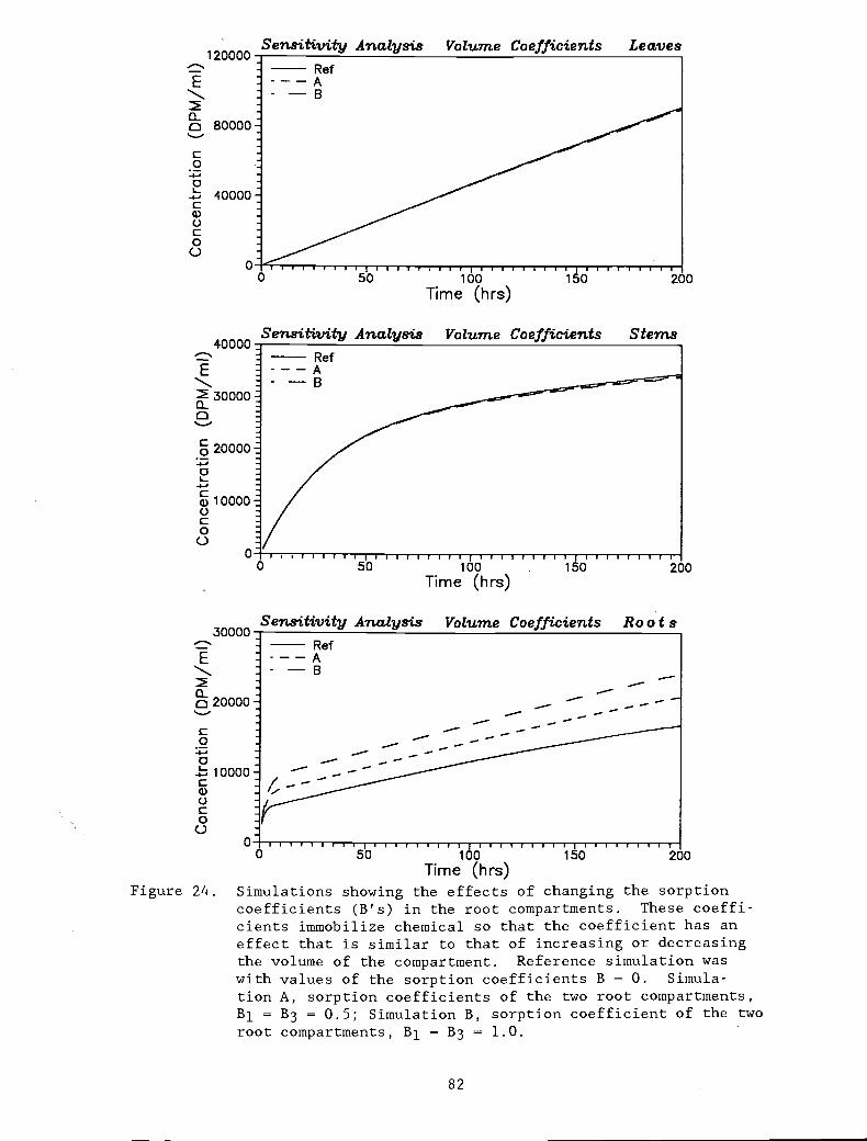
Sensitivtty Analysis Volume Coefficients120000
E
80000-
C0a
- 40000Ca)0C00
0
Sensitivity Analysis Volume Coefficients40000
E
30000 -
20000 -
jl0000_0
30000
E
20000
C0a-b 10000Ca)0C00
0
0
0
0
I-I I I TU I I I I I
50 100Time (hrs)
II I I I I ri III50 100
Time (hrs)
50
82
Leaves
Stems
200
111111111150 200
Sensitivity Analysis Volume Coefficients Ro o tsRefA- B
-
1''''100
Time (hrs)Figure 24 Simulations showing the effects of changing the sorption
coefficients (B's) in the root compartments. These coeffi-cients immobilize chemical so that the coefficient has aneffect that is similar to that of increasing or decreasingthe volume of the compartment. Reference simulation waswith values of the sorption coefficients B = 0. Simula-
tion A, sorption coefficients of the two root compartments,B1 = B3 = 0.5; Simulation B, sorption coefficient of the tworoot compartments, B1 = B3 = 1.0.
150 200THIS P
UBLICATIO
N IS O
UT OF D
ATE.
For mos
t curr
ent in
formati
on:
http:/
/exten
sion.o
regon
state.
edu/c
atalog

120000
E
80000
C00C0.)0C00
40000
E
30000
a
20000
110000
20000
E
15000:a.0
1100001
I0
Sensitiv%ty Analysis
510
Sensitivity Analysis
T-r rT I I I-I I
50 100Time (hrs)
Sensitivity Analysis Lambda's
100Time (hrs)
Lambda's
1T150
Stems
Root S
200
I-200
Ref---A--B- c
200100Time (hrs)
Figure 25. Simulations showing effects of changing the rates of first-order loss (A) in the leaves. Reference simulation waswith all A's equal to zero. Simulation A: AlS = 0.0016,
A18 = 0.00175, A21 = 0.0018; simulation B: A15 = 0.0032,
A18 = 0.0035, A21 = 0.0036; simulation C: A15 = 0.0064,
'18 = 0.0070, A21 0.0072.
83
LeavesLambda's
5b0
THIS P
UBLICATIO
N IS O
UT OF D
ATE.
For mos
t curr
ent in
formati
on:
http:/
/exten
sion.o
regon
state.
edu/c
atalog

Rate of First Order Losses
This simulation shows the result of allowing first-order loss
processes to operate. In the reference simulation, the rate of first-
order loss were zero in all compartments. For the simulation shown in
Figure 25, values of the coefficient, A, were as shown in Table 12.
Appendix I, equations (15), (18), and (21), indicate the role played by
this coefficient. The effects were most pronounced in the leaves,
which was expected since values were not changed in stem and root
compartments. An increase in the value of A has the effect of
decreasing the concentration. As there is less and less chemical
available in the leaves, the redistribution of the chemical by the
phloem pathway is affected so that, increasingly, the concentration in
the stem compartments shows a decrease. Concentrations in the root
compartments started to show a decrease as well.
Combined Effects
In conclusion of the limited set of sensitivity simulations, two
simulations were done in which several parameters were changed from the
reference data set at the same time. The sets of parameters for each of
these two simulations are in Table 13. Results are in Figures 26 and
27. The simulation in Figure 26 is labelled "combined high" and the
simulation in Figure 27 is labelled "combined low." This terminology
derived from the high concentrations with the simulation in Figure 27
and the low concentrations with the simulations in Figure 27.
The most influential parameter in these simulations was clearly the
diffusion coefficient at the Casparian strip. The diffusion coefficient
of the simulation labelled "combined high" was the lower of the two
84
THIS P
UBLICATIO
N IS O
UT OF D
ATE.
For mos
t curr
ent in
formati
on:
http:/
/exten
sion.o
regon
state.
edu/c
atalog

simulations and that was two orders of magnitude lower than with the
simulation referred to as "combined low." The diffusion coefficient at
the Casparian strip determines the rate of diffusion back to the
bathing solution of the root medium. With the high diffusion
coefficient, the rate of backward diffusion was high. This rate
increased as the concentration of the nutrient solution decreased. The
concentrations in all three plant parts approached a steady state with
the "combined low" simulation, whereas the concentrations of the
reference simulation and the "combined high" simulation continued to
increase. The lower rate of increase in the concentrations with the
"combined low" simulations was also in part caused by high value of
first-order loss rate in the leaves. The high concentrations in the
roots with the "combined high" simulations derived in part from high
value of the sorption coefficients in the root compartments. The very
low concentration in the stems of the "combined low" simulations
resulted from the very low value of the phloem/xylem transport rate and
the high reflection coefficient at the root surface.
85
THIS P
UBLICATIO
N IS O
UT OF D
ATE.
For mos
t curr
ent in
formati
on:
http:/
/exten
sion.o
regon
state.
edu/c
atalog

Table 13. Values of the parameters used for simulations in whichseveral parameters were changed for an evaluation of com-bined effects.
Transpiration (cm3/cm2/hr)
Phloem/xylem transport rate
Diffusion coefficient (cm2/hr)
Reflection coefficient, root
Reflection coefficient, leaf
Ratio: Qf/Qb
Sorption coefficient, root
First order loss rate,leaves
Tr = 8.85 x i0
f1=0.30; f2=O.20;f=0.lO
1.8 x 10⁻⁸
01 = 0.2
010=014=018=0. 7
Qf/Qb = 2 timesreference
Bi = B3 = 1.0
Al5 = 0.00160Al8 = 0.00175
0.00180
86
Tr = 7.82 x l0
f1=f2=f3=0 . 0
1.8 x 10⁻⁶
01 0.7
010=014=018=0. 2
Qf/Qb=0.50 timesreference
Bl = B3 = 0.5
A15 = 0.00640= 0.00700
A21 = 0.00720
Value of parametersSimulation in Simulation in
Parameter Fig. 26 Fig. 27
THIS P
UBLICATIO
N IS O
UT OF D
ATE.
For mos
t curr
ent in
formati
on:
http:/
/exten
sion.o
regon
state.
edu/c
atalog
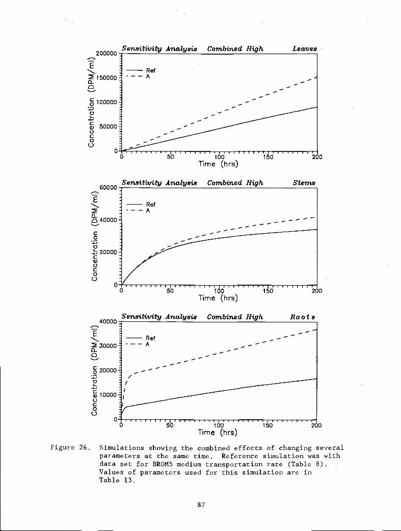
Sen.s-itivity Analysis200000
E
1500000a
110000050000 -
60000
E
40000
0a1
4-
U
000
RefA
Sensitivity Analysis
Combined High Leaves
100Time (hrs)
87
Combined High
150
Stems
Combined High Ro o t S
UTI iJ I0 50 100 150 200
Time (hrs)
Figure 26. Simulations showing the combined effects of changing severalparameters at the same time. Reference simulation was withdata set for BROM5 medium transportation rate (Table 8).Values of parameters used for this simulation are inTable 13.
Sensitivity Analysis40000
ERet---A
a30000
20000
j/
I
I I -
0 tlli I
0 50 150 200100Time (hrs)
THIS P
UBLICATIO
N IS O
UT OF D
ATE.
For mos
t curr
ent in
formati
on:
http:/
/exten
sion.o
regon
state.
edu/c
atalog

E
U-C)
c00Ca)000
40000
E
30000U-a
20000
110000
20000
Sensitiv'ty Analysis
0
0
E
15000-U-C)
I10000_500
Sensitivity Analysis
Sensitivity Analysis
Combined Low Stems
J I I I- I I l I
50 100Time (hrs)
Combined Low
I I
0 50 100Time (hrs)
Figure 27. Simulation showing the combined effects ofparameters Reference simulation was withBROM5 medium transpiration rate (Table 8).parameters used for this simulation are in
88
1 I I j I I I I I I I I
200150
Roots
id I I 1 I I I I1200
changing severaldata set forValues of
Table 13.
Combined Low Leaves
THIS P
UBLICATIO
N IS O
UT OF D
ATE.
For mos
t curr
ent in
formati
on:
http:/
/exten
sion.o
regon
state.
edu/c
atalog
CONCLUS IONS
The model satisfactorily predicted the observed uptake and distri-
bution patterns for bromacil in soybean plants at the stage of growth
and under the environmental conditions used in the experiments involv-
ing a range of transpiration rates. This indicates that the model
provides an accurate representation of uptake and the influence of
transpiration rate on the uptake and translocation of this chemical.
Parameter values used in the model for compartment size were selected
from literature and experimental observation. They functioned well in
these simulations and they are appropriately applied in the model. The
chemical parameters for storage, mobilization, and diffusion when used
in the model also yielded satisfactory results, suggesting that they
are also appropriately applied. Finally, the calibration, although of
limited scope, showed that the model equations yielded an accurate
picture of the actual UTAB patterns for bromacil in soybeans used in
these experiments. The theoretical exercise of compiling the model is
shown to be a constructive step in learning how to predict the fate of
xenobiotic contamination in plants.
The model shows excellent promise for future use. However, addi-
tional testing and validation are needed. Mathematical models can be
used productively in combination with experimental results to obtain
values of the unknown coefficients. Unfortunately, the parameters
which characterize compartments usually cannot be estimated uniquely
from "lumped" or "wash-out" type of experimental data when the number
of compartments exceeds two (Godfrey and diSteffano, 1987). When using
large system models for determination of unknown coefficients, experi-
ments must be carefully designed so that input/output information
89
THIS P
UBLICATIO
N IS O
UT OF D
ATE.
For mos
t curr
ent in
formati
on:
http:/
/exten
sion.o
regon
state.
edu/c
atalog

(variables) can be measured over time for fixed environmental condi-
tions. The input/output information so obtained would best be used in
an optimization scheme based on a nonlinear least squares or minimum
residual square error criterion to identify as many as possible of the
characterizing parameters. An optimization scheme could not be used
here because the data set was of the Iulumpedtt type. Data requirements
must be firmly kept in mind when contemplating use of models.
90
THIS P
UBLICATIO
N IS O
UT OF D
ATE.
For mos
t curr
ent in
formati
on:
http:/
/exten
sion.o
regon
state.
edu/c
atalog

LITERATURE CITED
Bard, Y. 1974. Nonlinear Parameter Estimation. Academic Press, New
York. 341 pp.
Berry, W. L. 1978. Nutrition, containers, and media. In: R. W.
Langhans, ed., A Growth Chamber Manual, Environmental Control for
Plants. Cornell University Press, Ithaca, NY. pp. 117-135.
Boersma, L., F. T. Lindstrom, C. McFarlane, and E. L. McCoy. 1988a.
Model of coupled transport of water and solutes in plants. Spec.
Report No. 818. Agric. Exp. Sta., Oregon State Univ., Corvallis.
109 p.
Boersma, L., F. T. Lindstrom, C. McFarlane, and E. L. McCoy. 1988b.
Uptake of organic chemicals by plants: A theoretical model. Soil
Science 146:403-417.
Boersma, L., F. T. Lindstrom, C. McFarlane, and K. P. Suen. l988c.
User Guide: Uptake and transport of chemical by plants; thee leaf
model. Spec. Report No. 819. Agric. Exp. Sta., Oregon State
Univ., Corvallis. 79 p.
Box, C. E. P., W. C. Hunter, and J. S. Hunter. 1978. Statistics for
Experiments: An Introduction to Design, Data Analysis, and Model
Building. Wiley, New York. 633 pp.
Boyce, W. E. and R. C. DiPrima. 1965. Elementary Differential Equa-
tions and Boundary Value Problems. John Wiley and Sons, New York.
485 pp.
Christy, A. L. and J. M. Ferrier. 1973. A mathematical treatment of
Munch's pressure-flow hypothesis of phloem translocation. Plant
Physiol. 52:531-538.
91
THIS P
UBLICATIO
N IS O
UT OF D
ATE.
For mos
t curr
ent in
formati
on:
http:/
/exten
sion.o
regon
state.
edu/c
atalog

Eschich, W., R. F. Evert, and J. H. Young. 1972. Solution Flow in
Tubular Semipermeable Membranes. Planta 107:279-300.
Ferrier, J. M. and A. L. Christy. 1975. Time-dependent behavior of a
mathematical model of Munch translocation. Plant Physiol. 55:511-
514.
Godfrey, K. R. and J. J. diSteffano, III. 1987. Identifiability of
model parameters. In: E. Walter, ed., Identifiability of Paramet-
ric Models. Pergamon Press, Oxford. 119 pp.
Goeschl, J. D., C. E. Magnuson, D. W. DeMichele, and P. J. H. Sharpe.
1976. Concentration-dependent unloading as a necessary assumption
for a closed form mathematical model of osmotically driven pres-
sure flow in phloem. Plant Physiol. 58:556-562.
Golub, C. H. and C. F. Van Loam. 1983. Matrix Computations. Johns
Hopkins University Press, Baltimore. 476 p.
Jachetta, J. J., A. P. Appleby, and L. Boersma. 1986a. Use of the
pressure vessel to measure concentrations of solutes in apoplastic
and membrane-filtered symplastic sap in sunflower leaves. Plant
Physiol. 82:995-999.
Jachetta, J. J., A. P. Appleby, and L. Boersma. l986b. Apoplastic and
symplastic pathways of atrazine and glyphosate transport in shoots
of seedling sunflower. Plant Physiol. 82:1000-1007.
Jacquez, J. A. 1972. Compartmental Analysis in Biology and Medicine.
Elsevier, Amsterdam. 237 p.
McCrady, J. K., C. McFarlane, and F. T. Lindstrom. 1987. The
transport and affinity of substituted benzenes in soybeans. J.
Expt. Bot. 38:1875-1890.
92
THIS P
UBLICATIO
N IS O
UT OF D
ATE.
For mos
t curr
ent in
formati
on:
http:/
/exten
sion.o
regon
state.
edu/c
atalog

McFarlane, J. C. and T. Pfleeger. 1986. Plant exposure laboratory and
chambers, Vol. 1. EPA-600/3-86-007a. USEPA, Corvallis, OR.
McFarlane, J. C. and T. Pfleeger. 1987. Plant exposure chambers for
study of toxic chemical-plant interactions. J. Environ. Qual.
16(6):361-371.
McFarlane, C., C. Nolt, C. Wickliff, T. Pfleeger, R. Shimabuku, and M.
McDowell. 1987. The uptake, distribution and metabolism of four
organic chemicals by soybean plants and barley roots. Environ.
Tox. and Chem. 6:847-856.
Moler, C. B. and C. F. Van Loan. 1978. Nineteen dubious ways to
compute the exponential of a matrix. SIAM Review 20:801-836.
Nobel, P. S. 1983. Biophysical Plant Physiology and Ecology. W. H.
Freeman and Company, New York, NY. 608 pp.
Seagrave, R. C. 1971. Biomedical Applications of Heat and Mass
Transfer. Iowa State Univ. Press, Ames, Iowa. 175 pp.
Tyree, M. T., C. A. Peterson, and L. V. Edgington. 1979. A simple
theory regarding ambimobility of xenobiotics with special refer-
ence to the nematicide, oxamyl. Plant Physiol. 63:367-374.
Varga, R. S. 1962. Matrix Iterative Analysis. Prentice-Hall,
Englewood Cliffs, NJ. 322 p.
Ward, R. C. 1977. Numerical Computation of the matrix exponential
with accuracy estimates. SIAM J. Num. Anal. 14:600-614.
Weir, G. J. 1981. Analysis of Munch theory. Math. Biosci. 56:141-
152.
93
THIS P
UBLICATIO
N IS O
UT OF D
ATE.
For mos
t curr
ent in
formati
on:
http:/
/exten
sion.o
regon
state.
edu/c
atalog

APPENDIX 1
DEFINITIONS OF THE NON-ZERO COEFFICIENTS, ajj.
-1) Soil compartment
cTht
dt= a11 M1 + a10 M0
1D0A0 D0A0
LX0i
Lx0=
- IC V(l + B1) +
0) Root free space compartment
dM0= a1 M1 + a00 M0 + a01 M1 + a02 M2
D0A0+
a01= e(1 + B1) V1
1D0A0 D1A1ST 1
I + 1
+ Qf0 + Q (1 - a )1 1 Ia00 = -
I V0(1 + B0)+
STbo
D1 A1a01
= V1(l + B1)'a02
= V2(1 + B2)
Root exterior cells compartment
dM1
a10 M0 + a11 M1
ST STQf0 b0a10
= V0(1 + B0)'a11
= -[V1(1 + B1) +
94
= V0(l + B0)
THIS P
UBLICATIO
N IS O
UT OF D
ATE.
For mos
t curr
ent in
formati
on:
http:/
/exten
sion.o
regon
state.
edu/c
atalog

2) Root xylem compartment
a20
dM2
dt= a20 M0 + a22 M2 a23 M3 + a24 M4 + A25 M5
D1 A1+ - a1)
V0(1 + B0)
1D1 A1 D4 A4 D2 A2ST.
Ix1 + x4 + x2
+ Q2(l - a2) + Qf1
a22 =* L V2(l + B2) +
ST
1a23= V3(l + B3)'
D2 A2
a25V5(l + B5)
3) Root storage compartment
dM3
= a32 M2 + a33 M3 + a34 Fl4
ST ST STQf1 bl + b2a32
= V2(l + B2)'a33 =
- V3(l + B3)+ A3
STQf2
a34= V4(1 + B4)
a24 =
D4 A4+ Q4(l - a4)
x4
V4(l + B4)
95
THIS P
UBLICATIO
N IS O
UT OF D
ATE.
For mos
t curr
ent in
formati
on:
http:/
/exten
sion.o
regon
state.
edu/c
atalog
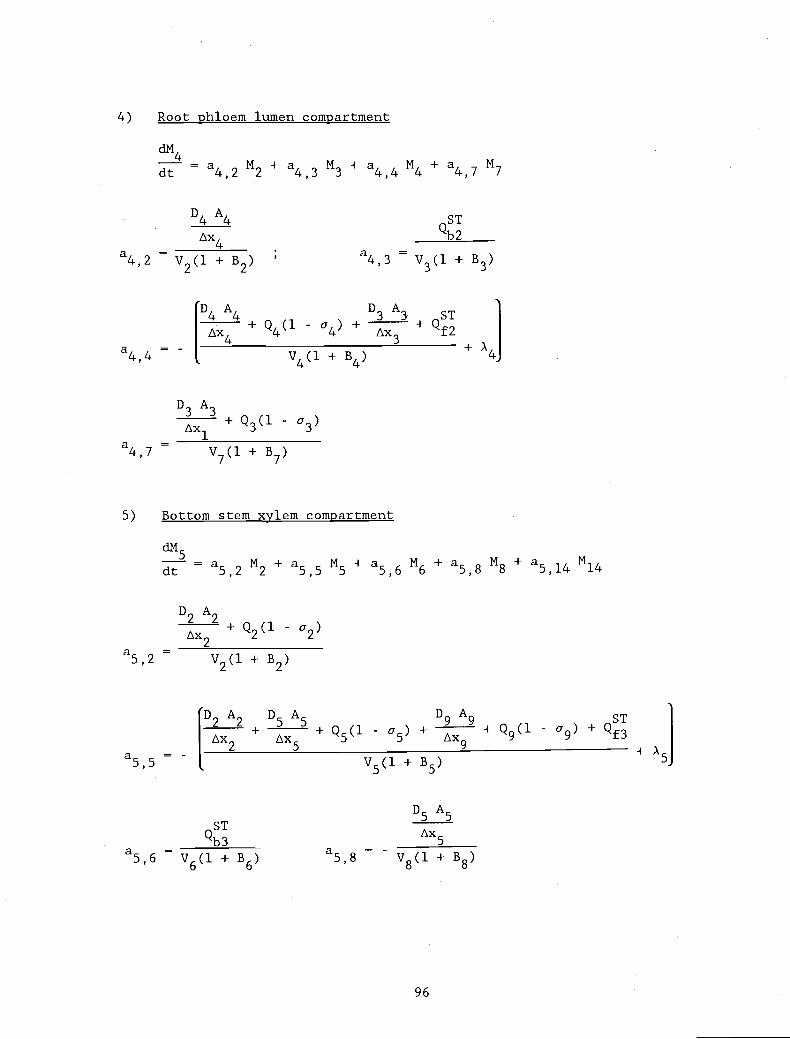
4) Root phloem lumen compartment
dM,,
= a42 M2 + a43 M3 + a44 M4 + a47 M7
D4A4ST
Ax4a42
= V2(l + B2)a43
= V3(l + B3)
a5
a44 = -
Ax1
ID4 A4 D3 A3ST
Ax4+ Q(l - c74)
+ Ax3 + Qf2
V4(l + B4)
D3 A3+ Q3(l - 73)
4]
[D2 A2 D5 A5 D9 A9 ST
Ax2 + A+ Q5(l - a5)
+ A+ Q9(l - a9) + Qf3
V5(l + B5)+ A5J
ST3a56
- V6(l + B6)a58 =
D5 A5
Ax5
V8(l + B8)
96
5) Bottom stem xylem compartment
dM5
=a52M2+a55M5+a56M6+a58M8+a5,14M14
D2 A2+ Q2(l - a2)
a47 =V7(1 + B7)
a52 =V2(l + B2)
THIS P
UBLICATIO
N IS O
UT OF D
ATE.
For mos
t curr
ent in
formati
on:
http:/
/exten
sion.o
regon
state.
edu/c
atalog
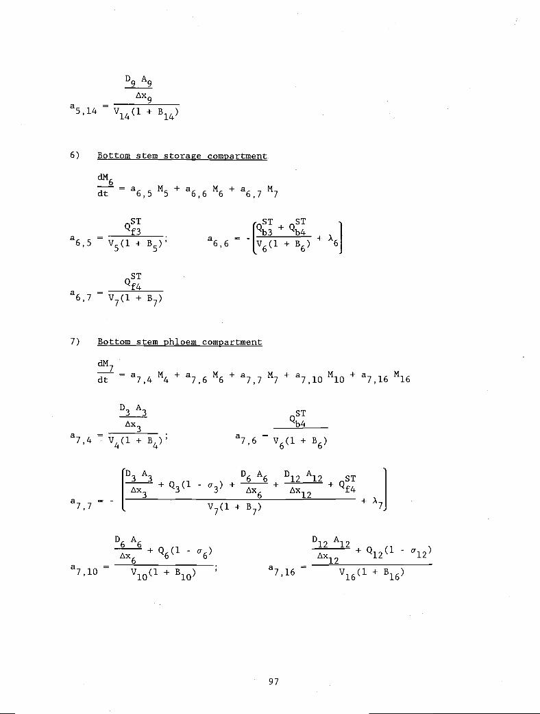
7) Bottom stem phloem compartment
dM= a4 M4 + a76 M6 + a77 M7 + a710 M10 + a716 M16
D3A3ST
b4a74
V4(1 + B4)'a76
= V6(1 + B6)
[D3 A3 D6 A6 D12 Al2ST
+ Q(1 - a3)+
++ Qf4
a77 =- V7(1 + B7)
+ A7J
D6 A6+ Q6(1 - a6)
97
D12 Al2+ - a12)
a514
6)
D9 A9
1x9
= V14(1 + B14
Bottom stem storage compartment
dM
M7= a65 M5 + a66 M6 + a67
ST ST STQf3 1b3 + b4a65
= V5(1 + B5)'a66
+ B6)+ A6
STQf4
a67V7(1 + B7)
a7, 10 + B10)
a716 =V16(1 + B16)
THIS P
UBLICATIO
N IS O
UT OF D
ATE.
For mos
t curr
ent in
formati
on:
http:/
/exten
sion.o
regon
state.
edu/c
atalog

8) Mid stem xylem lumen compartment
= a85 M5 + a88 M8 + a89 M9 + a811 M11 + a817 M17
D5 A5+ Q5(l - a5)
ID3 A3 D7 A7 D13 A13 ST
I+ + Q7(17)+ l3
+ Q13(a13) + Qf5
a88 = - V8(1 + B8)+ A8j
D7 A7
ST
bsIx7
a89= V9(l + B9)
a811 V11(1 + B11)
D13 A13
x13a817
= V17(l + B17)
9) Mid stem storage compartment
aM0a98 M8 + a99 M9 + a910 M10
a98 =
ST ST STQf5 1b5 + b6
(1 + B8)'a99
= ivg(1 + B9) +A9
STQf6
a910= V10(1 + B10)
98
a85 =V5(l + B5)
THIS P
UBLICATIO
N IS O
UT OF D
ATE.
For mos
t curr
ent in
formati
on:
http:/
/exten
sion.o
regon
state.
edu/c
atalog

10) Mid stem phloem lumen compartment
dM10
dt = a107 M7 + a109 M9 a1010 M10 + a1013 M13 + a1019 M19
D6 A6
a107= V7(1+ B7)
a1010
D8 A8 D16 A16+ Q8(l - a8)
l6
+ Q16(1 - cr16)
a1013V13(1 + B13) a1019
= V16(1 + B16)
11) Top stem xylem lumen compartment
dM11
dt a118 M8 + a1111 M11 + a1112 M12 + a1120 M20
a118 =
a1111 =
[D8 A8 D6 A6 D16 A16ST
10]
Ax8 + Ax6+ - Or)
+ Ax16 + Qf6= +
V10(1 + B10)
D7 A7
Ax7+ Q7(1 - a7)
V8(1 + B8)
ID7
A7D17 A17ST
Ax7 + Ax17 + Q17(1 - a17) + Qf7
V11(1 + B11)
STb7 Ax17
a1112V12(l + B12)' a11,20
= V20(1 + B20)
STb6
a109= V9(1 + B9)
99
D17 A17THIS
PUBLIC
ATION IS
OUT O
F DATE.
For mos
t curr
ent in
formati
on:
http:/
/exten
sion.o
regon
state.
edu/c
atalog
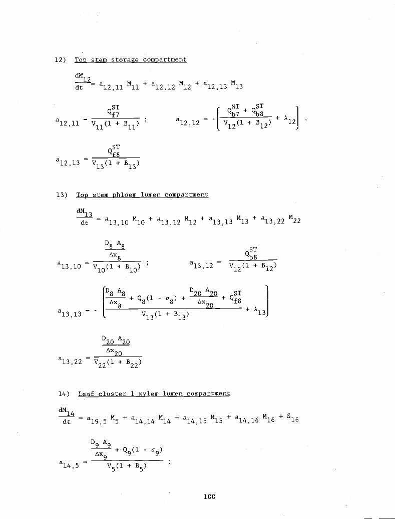
12) Top stem storage compartment
12
dt= a1211 M11 + a1212 M12 + a1213 M13
ST ST STQf7 b7 + b8
a1211 = V11(1 + B11)a1212 =
- V12(1 + B12)+ Al2
a1213
13) Top stem phloem lumen compartment
3
dt= a1310 M10 + a1312 M12 + a1313 M13 + a1322 M22
a13,10 V10(l + B10)
ID8 A8 D20 A20ST
I8
+ Q8(1 - &8)+ 2O
+ Qf8
a1313 =- V13(1 + B13)
+ A13J
D20 A20
Lx20
a1322 = V22(l + B22)
14) Leaf cluster 1 xylem lumen compartment
l4 =adt 19,5
M5 + a1414 M14 + a1415 M15 + a1416 M16 + S16
D9 A9+ Q9(1 - a9)
STQf8
13(1 + B13)
D8 A8
Lx8ST8
a1312 = v12(l + B12)
100
a145 =V5(1 + B5)
THIS P
UBLICATIO
N IS O
UT OF D
ATE.
For mos
t curr
ent in
formati
on:
http:/
/exten
sion.o
regon
state.
edu/c
atalog
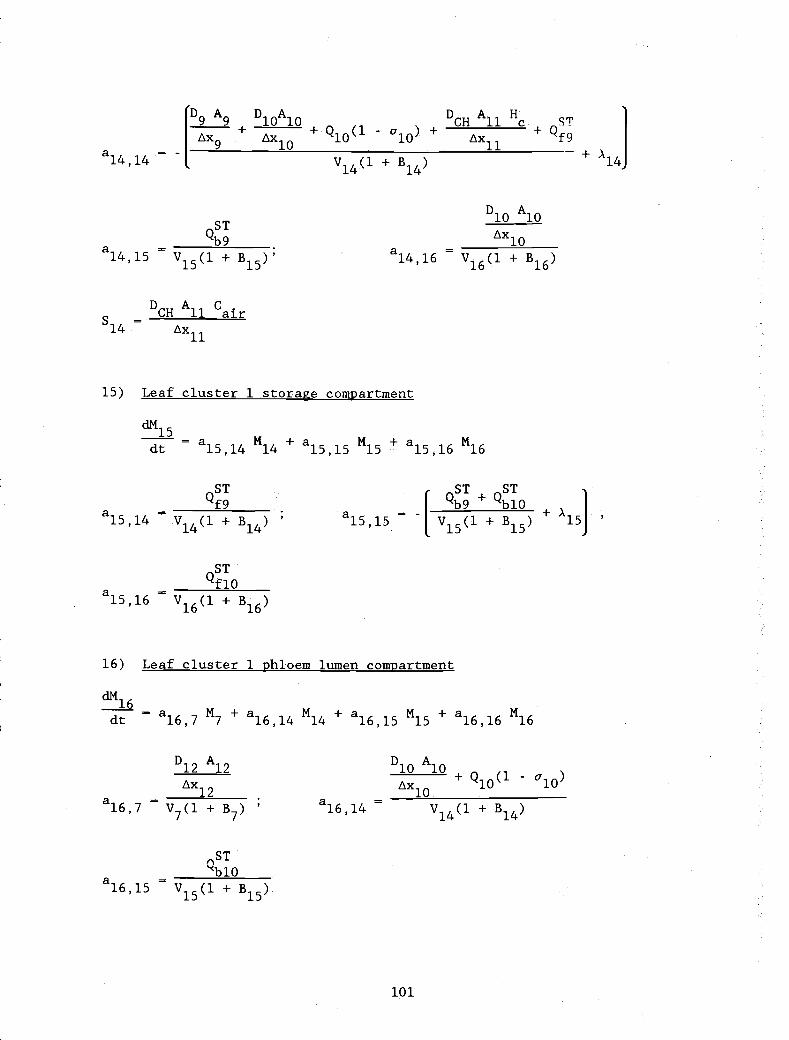
D9 A9 D10A10 DCH A11 HST
Ax9 + Ax10+ Q10(1 - a10)
+ Ax11 + Qf9
Aa1414 -- V14(1 + B14) + 14
ST
9a1415= V15(l + B15)'
DCH A11 Cair
Ax
15) Leaf cluster 1 storage compartment
dM15
dt= a1514 M14 + a1515 M15 + a1516 M16
ST ST STQf9 b9 + b10a1514
V14(1 + B14)' a15,15- V15(1 + B15)
+ A15
STQf10
a1516= V1(1 + B16)
16) Leaf cluster 1 phloem lumen compartment
dM16= a167 M7 + a1614 M14 + a1615 M15 + a1616 M16
11
D12 Al2
Ax12a167
= V7(l + B7
ST
10a1615= V15(1 +
a1614 =
a1416
D10 A10
Ax + - a10)
101
D10 A10
Ax10
(1 + B16)
10 -
+ B14)THIS
PUBLIC
ATION IS
OUT O
F DATE.
For mos
t curr
ent in
formati
on:
http:/
/exten
sion.o
regon
state.
edu/c
atalog

ID10 A10 D12 Al2 ST
I ++ Q12(1 - a12) + Qf10
a1616 =v16(1 + B16)
17) Leaf 2 cluster xylem lumen compartment
7
dt= a178 M8 + a1717 M17 + a1718 M18 + a1719 M19 +
a17, 8
D13 A13
Ax13+ Q13(1 - a13)
V8(1 + B8)
ID13 A13 D14 A14 DCH H A15STI+ 14
+ Q14(1 - a14) + Ax15 + Qf11
a1717 = V17(1 + B17)+
D14 A14
ST
b11Ax14
a1718= V18(1 + B18)'
a1719 V19(1 + B19)
DCHA1 C5 air
Ax15
18) Leaf 2 cluster storage compartment
18
dt= a1817 M17 + a1818 M18 + a1819 M19
102
STQf11
a1817= V17(1 + B17)
a1818
STQf12
a1819= V19(1 + B19
ST
b11 +ST
b12=
- v18(1 + B18) +A18
THIS P
UBLICATIO
N IS O
UT OF D
ATE.
For mos
t curr
ent in
formati
on:
http:/
/exten
sion.o
regon
state.
edu/c
atalog

19) Leaf 2 cluster phloem lumen compartment
9
dta1910 M10 + a1917 N17 + a1918 M18 + a1919 M19
D16 A16 D14 A14
Ax16 Ax14+ Q14(l
-
a1910= V10(l + B10)'
a1917V17(l + B17)
STQf12
a1918= V18(l + B18)
Ax16+ Q16(1 - a16)
+ Ax14 +
[D16 A16 D14 A14
a1919- V19(1 + B19)
+ A19J
20J
D A C.('i-I 1Q air
=
103
20) Leaf 3 cluster xylem lumen compartment
+
0a2011 M11 + a2020 M20 + a2021 M21 a2022 N22 + S20
D17 A17
dt=
a2011
a2020
a2021
Ax17+ Q17(1 - a17)
-
V11(1 + B11)
ID17 A17 D18 A18 DCH Hc A19 STAx18
+ Q18(- - a18) + Ax19 + Qf13
V20(l + B20)
D18 A18ST
b13Ax18
= V21(1 + B21)' a2022 = V22(l + B22)
THIS P
UBLICATIO
N IS O
UT OF D
ATE.
For mos
t curr
ent in
formati
on:
http:/
/exten
sion.o
regon
state.
edu/c
atalog

21) Leaf 3 cluster storage compartment
1
dt= a2120 N20 + a2121 M21 + a2122 M22
ST ST STQf13
[bl3 + bl4
a2120 = V20(l + B20)a2121
=V2(l + B21)
+ A21]
STQf14
a2122 = V22(1 + B22)
22) Leaf 3 cluster phloem lumen compartment
dMzL = a213 M13 + a2220 N20 + a2221 M21 + a2222 M22
D20 A20
a2213 = V13(1 + B13)'
STb14
a2221 = V21(1 + B21)
a2222 -
D18 A18+ - a18)
LX18
a2220 = V20(1 + B20)
I'2o A20 D18 A18ST
[
tx20+ Q20(1
-a20)
++ Qf14
V(1 + B99)
104
+ A2j
THIS P
UBLICATIO
N IS O
UT OF D
ATE.
For mos
t curr
ent in
formati
on:
http:/
/exten
sion.o
regon
state.
edu/c
atalog