model and quality driven embedded systems engineering · 3 eila ovaska, andrÆs balogh, sergio...
TRANSCRIPT
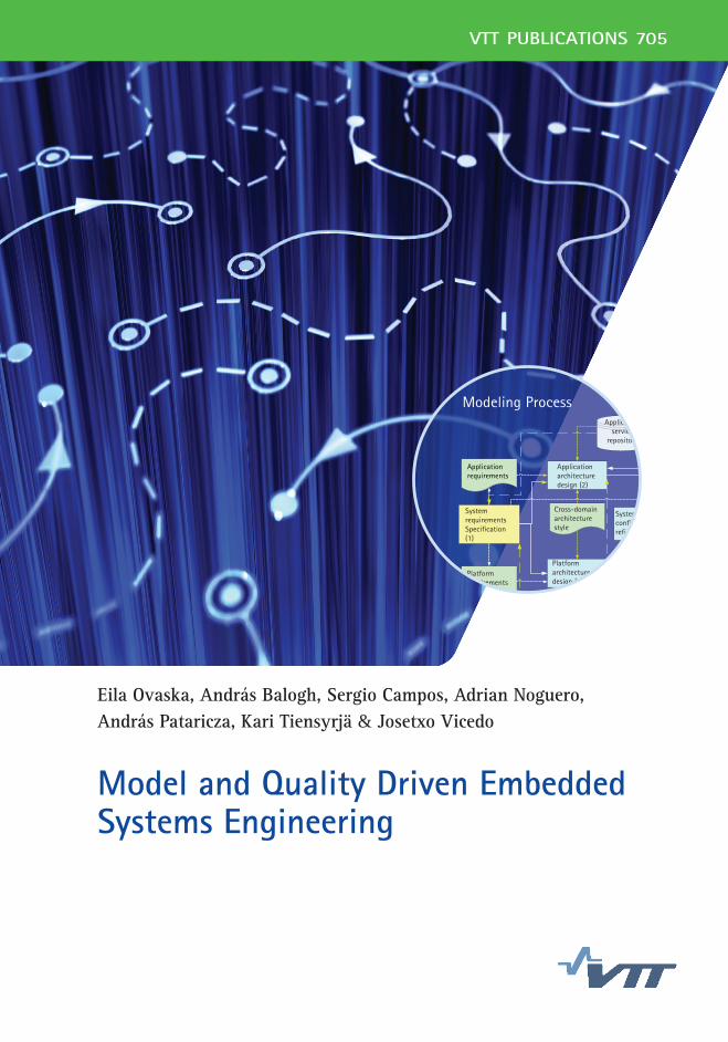
Modeling Process
Applicationrequirements
SystemrequirementsSpecification(1)
Platformrequirements
Referencearchitecturetemplate
Platformmodule library
Platformarchitecturedesign (3)
Cross-domainarchitecturestyle
Applicationarchitecturedesign (2)
Applicationservice
repository
System allocation/configuration/ refinement (4)
Qualityevaluation (5)
Realization(HW/SW)(6)
Evaluationcriteria
Validated systemArchitecture
models
VTT PUBLICATIONS 705VTT CREATES BUSINESS FROM TECHNOLOGY Technology and market foresight • Strategic research • Product and service development • IPR and licensing • Assessments, testing, inspection, certifi cation • Technology and innovation management • Technology partnership
• • • VTT PUB
LICA
TION
S 705 MO
DEL A
ND
QU
ALITY D
RIVEN
EMB
EDD
ED SYSTEM
S ENG
INEER
ING
ISBN 978-951-38-7336-3 (URL: http://www.vtt.fi /publications/index.jsp)ISSN 1455-0849 (URL: http://www.vtt.fi /publications/index.jsp)
Eila Ovaska, András Balogh, Sergio Campos, Adrian Noguero, András Pataricza, Kari Tiensyrjä & Josetxo Vicedo
Model and Quality Driven Embedded Systems Engineering
VTT PUBLICATIONS
692 Kimmo Keränen. Photonic module integration based on silicon, ceramic and plastic technologies. 2008. 101 p. + app. 70 p.
693 Emilia Selinheimo. Tyrosinase and laccase as novel crosslinking tools for food biopolymers. 2008. 114 p. + app. 62 p.
694 Olli-Pekka Puolitaival. Adapting model-based testing to agile context. 2008. 69 p. + app. 6 p.
695 Minna Pikkarainen. Towards a Framework for Improving Software Development Process Mediated with CMMI Goals and Agile Practices. 2008. 119 p. + app. 193 p.
696 Suvi T. Häkkinen. A functional genomics approach to the study of alkaloid biosynthesis and metabolism in Nicotiana tabacum and Hyoscyamus muticus cell cultures. 2008. 90 p. + app. 49 p.
697 Riitta Partanen. Mobility and oxidative stability in plasticised food matrices. The role of water. 2008. 92 p. + app. 43 p.
698 Mikko Karppinen. High bit-rate optical interconnects on printed wiring board. Micro-optics and hybrid integration. 2008. 162 p.
699 Frej Wasastjerna. Using MCNP for fusion neutronics. 2008. 68 p. + app. 136 p.
700 Teemu Reiman, Elina Pietikäinen & Pia Oedewald. Turvallisuuskulttuuri. Teoria ja arviointi. 2008. 106 s.
701 Pekka Pursula. Analysis and Design of UHF and Millimetre Wave Radio Frequency Identifi cation. 2008. 82 p. + app. 51 p.
702 Leena Korkiala-Tanttu. Calculation method for permanent deformation of unbound pavement materials. 2008. 92 p. + app. 84 p.
703 Lauri Kurki & Ralf Marbach. Radiative transfer studies and Next-Generation NIR probe prototype. 2009. 43 p.
704 Anne Heikkilä. Multipoint-NIR-measurements in pharmaceutical powder applications. 2008. 60 p.
705 Eila Ovaska, András Balogh, Sergio Campos, Adrian Noguero, András Pataricza, Kari Tiensyrjä & Josetxo Vicedo. Model and Quality Driven Embedded Systems Engineering. 2009. 208 p.

VTT PUBLICATIONS 705
Model and Quality Driven Embedded Systems Engineering
Eila Ovaska & Kari Tiensyrjä VTT Technical Research Centre of Finland
Sergio Campos, Adrian Noguero & Josetxo Vicedo European Software Institute (ESI)
András Balogh & András Pataricza Budapest University of Technology and Economics (BME)

ISBN 978-951-38-7336-3 (URL: http://www.vtt.fi/publications/index.jsp) ISSN 1455-0849 (URL: http://www.vtt.fi/publications/index.jsp)
Copyright © VTT 2009
JULKAISIJA � UTGIVARE � PUBLISHER
VTT, Vuorimiehentie 5, PL 1000, 02044 VTT puh. vaihde 020 722 111, faksi 020 722 7001
VTT, Bergsmansvägen 5, PB 1000, 02044 VTT tel. växel 020 722 111, fax 020 722 7001
VTT Technical Research Centre of Finland, Vuorimiehentie 5, P.O. Box 1000, FI-02044 VTT, Finland phone internat. +358 20 722 111, fax +358 20 722 7001
Technical editing Leena Ukskoski Text preparing Tarja Haapalainen

3
Eila Ovaska, András Balogh, Sergio Campos, Adrian Noguero, András Pataricza, Kari Tiensyrjä &Josetxo Vicedo. Model and Quality Driven Embedded Systems Engineering. Espoo 2009. VTTPublications 705. 208 p.
Keywords methodology, modelling, evaluation, quality, embedded systems engineering
Abstract The world of embedded systems is broad and diverse, addressing a wide variety of application domains. Although technologically, the situation for embedded systems is still quite fragmented, platform-based engineering, reference designs and maturing system domains have effected great changes. However, the features of modern embedded systems are changing at such a rate that it is increasingly difficult for companies to bring new products to the market within acceptable time scales and still guarantee acceptable levels of operational quality. This report aims for its part to increase the convergence of views with regard to embedded systems technologies and engineering methods.
The objective of this report is to introduce the methodology framework for model and quality driven embedded systems engineering. The framework is composed of three key artefacts, which provide the basis for building specific methodology instances. While instantiating this methodology framework, it has to be adapted to the needs and constraints of that specific application domain and development organisation.
The first key artefact of the methodology framework is the process model, the Y-chart model. The second key artefact is the Unified Modelling Language (UML) adapted to embedded systems engineering with a specific profile. The third key artefact consists of a set of evaluation methods that have been selected for use in embedded system engineering. Within the conclusions, an initial integrated development environment is introduced for embedded systems engineering.
The methods selected for the methodology framework have been validated in different application domains of embedded or/and software systems engineering areas.
4
Foreword This report is related to the European joint undertaking, called ARTEMIS (Advanced Research & Technology for EMbedded Intelligence and Systems), in the arena of embedded intelligence and systems engineering. The vision of ARTEMIS is that embedded systems will realise ambient intelligence in the physical objects of our everyday life and also in large-scale applications. By these means, ARTEMIS will increase the quality of people�s lives by making life healthier, more secure and by providing more comfort for Europe�s ageing population. Moreover, ARTEMIS aims to strengthen Europe�s position in embedded intelligence and systems and to attain world-class leadership in this area.
This report introduces the first results of the methodology framework research made in one work package of the GENESYS (GENeric Embedded SYStem platform, FP7-213322) project [GENESYS 2008], which is an EU-funded effort to tackle the challenges of future embedded systems defined in ARTEMIS-SRA (http://www.artemis-sra.eu/). The work was done in collaboration with researchers from VTT, European Software Institute (ESI) and Budapest University of Technology and Economics (BME).
I would like to thank Professor Veikko Seppänen from the University of Oulu for his insights and valuable comments for improving this report.
I hope that readers in future ARTEMIS projects and more broadly in embedded systems engineering will find this report to be both interesting and useful.
January 2009
Eila Ovaska Research Professor Leader of the Methodology and Tools work package in the GENESYS project

5
Contents
Abstract ................................................................................................................3
Foreword ............................................................................................................... 4
Key Abbreviations ................................................................................................. 9
Part 1. Introduction ........................................................................................... 12 1.1 Overview........................................................................................................................... 12 1.2 Definitions ......................................................................................................................... 13
1.2.1 Methodology Framework........................................................................................ 13 1.2.2 Domain................................................................................................................... 14 1.2.3 The Cross-domain Style and Template ................................................................. 14 1.2.4 Embedded System................................................................................................. 15 1.2.5 Service Description ................................................................................................ 15 1.2.6 Service Modelling................................................................................................... 15 1.2.7 Ontology................................................................................................................. 16 1.2.8 Dependability ......................................................................................................... 16
1.2.8.1 Safety......................................................................................................... 17 1.2.8.2 Reliability.................................................................................................... 18 1.2.8.3 Availability .................................................................................................. 19 1.2.8.4 Security ...................................................................................................... 19
1.2.9 Scalability ............................................................................................................... 20 1.2.10 Performance ....................................................................................................... 20 1.2.11 Evolvability .......................................................................................................... 20 1.2.12 Quality of Service (QoS) ..................................................................................... 20
1.3 Principles of the Methodology Framework........................................................................ 21 1.3.1 Embedded Systems Engineering Process............................................................. 21 1.3.2 Model Driven Development.................................................................................... 22 1.3.3 Model Representation............................................................................................ 22 1.3.4 Modelling Semantics.............................................................................................. 23 1.3.5 Formal Methods ..................................................................................................... 23 1.3.6 Quality and Non-Functional Properties .................................................................. 24 1.3.7 Support for Early V&V............................................................................................ 24 1.3.8 Integrated Development Environment ................................................................... 24

6
Part 2. Process Model ...................................................................................... 26 2.1 Overview........................................................................................................................... 26 2.2 Process Phases ................................................................................................................ 28
2.2.1 System Requirements Specification ...................................................................... 28 2.2.2 Application Architecture Design ............................................................................. 29 2.2.3 Platform Architecture Design ................................................................................. 30 2.2.4 System Allocation / Configuration / Refinement..................................................... 31 2.2.5 Quality Evaluation .................................................................................................. 31 2.2.6 System Realization ................................................................................................ 32
2.3 Artefacts............................................................................................................................ 33
Part 3. Modelling and Evaluation...................................................................... 35 3.1 System Requirements Specification ................................................................................. 35
3.1.1 Requirements Elicitation ........................................................................................ 37 3.1.2 Requirements Analysis and Documentation .......................................................... 38 3.1.3 Requirements Traceability ..................................................................................... 41
3.2 Architecture Design........................................................................................................... 41 3.2.1 Selection of Modelling Languages ......................................................................... 42 3.2.2 Architectural Elements ........................................................................................... 46 3.2.3 Architectural Views, Models and Transformations................................................. 47
3.3 Application Architecture Design ........................................................................................ 48 3.3.1 Structural View....................................................................................................... 50 3.3.2 Syntactical View..................................................................................................... 55 3.3.3 Behaviour View ...................................................................................................... 58 3.3.4 Semantic View ....................................................................................................... 62
3.4 Platform Architecture Design ............................................................................................ 63 3.4.1 Structural View....................................................................................................... 65
3.4.1.1 MARTE GRM Concepts for Execution Platform Modelling........................ 66 3.4.1.2 Modelling Processing Units and Tasks...................................................... 68 3.4.1.3 Modelling Shared Resources..................................................................... 69 3.4.1.4 Modelling Variables and Shared Memory .................................................. 70 3.4.1.5 Modelling Communication Resources ....................................................... 70 3.4.1.6 Modelling Platform Black-boxes................................................................. 71 3.4.1.7 Modelling Timing Resources...................................................................... 72 3.4.1.8 Further Refining Platform Structural Models.............................................. 73
3.4.2 Behaviour View ...................................................................................................... 73 3.4.3 Code View.............................................................................................................. 76
3.5 Platform Module Library.................................................................................................... 77 3.6 Integration and Development of Platform Services .......................................................... 79
3.6.1 Interfacing with Platform Services.......................................................................... 79 3.6.2 Describing the Behaviour of the Services .............................................................. 80 3.6.3 Design Process for New Platform Services ........................................................... 80
3.7 System Allocation / Configuration / Refinement ............................................................... 81 3.7.1 Schedulability Analysis and Simulation.................................................................. 83
3.7.1.1 Scheduling View ........................................................................................ 83 3.7.1.2 Analysis and Simulation Tools ................................................................... 87
7
3.7.1.3 Concepts of Scheduling View .................................................................... 95 3.8 Quality Evaluation ............................................................................................................. 97
3.8.1 Performance Evaluation......................................................................................... 98 3.8.1.1 Pre-requisites........................................................................................... 100 3.8.1.2 System Requirements Definition.............................................................. 100 3.8.1.3 Application Architecture Design ............................................................... 101 3.8.1.4 Platform Architecture Design ................................................................... 102 3.8.1.5 System Allocation / Configuration / Refinement....................................... 103
3.8.2 Performance Evaluation Methods........................................................................ 104 3.8.2.1 Performance Evaluation of Software Architecture ................................... 105 3.8.2.2 Application-platform Performance Evaluation.......................................... 108
3.8.3 Power/Energy Efficiency Evaluation .................................................................... 117 3.8.3.1 Pre-requisites........................................................................................... 118 3.8.3.2 System Requirements Definition.............................................................. 118 3.8.3.3 Application Architecture Design ............................................................... 119 3.8.3.4 Platform Architecture Design ................................................................... 120 3.8.3.5 System Allocation / Configuration / Refinement....................................... 120
3.8.4 Power/Energy Evaluation Techniques ................................................................. 120 3.8.4.1 Power Analysis in a Multiprocessor Simulation Platform......................... 121
3.8.5 Reliability and Availability Evaluation................................................................... 124 3.8.5.1 System Requirements Specification ........................................................ 125 3.8.5.2 Architecture Design.................................................................................. 128
3.8.6 Reliability and Availability Evaluation Methods .................................................... 130 3.8.6.1 Reliability Prediction of Component Based Architectures........................ 130 3.8.6.2 Reliability Evaluation in Model Driven Development................................ 132 3.8.6.3 Reliability and Availability Prediction and Testing.................................... 135 3.8.6.4 Commercial Reliability Analysis Tools ..................................................... 136
3.8.7 Safety Analysis..................................................................................................... 137 3.8.7.1 Safety Analysis Techniques..................................................................... 138 3.8.7.2 GENESYS Safety Certification Approach................................................ 143 3.8.7.3 Prerequisites ............................................................................................ 145 3.8.7.4 System Requirements Specification ........................................................ 146 3.8.7.5 Fault and Hazard Modelling ..................................................................... 148
3.8.8 Safety Analysis Methods (PSSA Stage) .............................................................. 150 3.8.8.1 Hip-HOPS Method ................................................................................... 151 3.8.8.2 Model Checking Method .......................................................................... 155 3.8.8.3 Commercial Safety Analysis Tools .......................................................... 158
3.8.9 Composability Evaluation..................................................................................... 158 3.8.9.1 Model-Based Evaluation .......................................................................... 160 3.8.9.2 Component Based Evaluation ................................................................. 163
3.8.10 Evolvability Evaluation ...................................................................................... 166 3.8.10.1 Adaptability Evaluation............................................................................. 167 3.8.10.2 Extensibility Evaluation ............................................................................ 170 3.8.10.3 Maintainability, Flexibility and Modifiability Evaluation............................. 172 3.8.10.4 Trade-off Analysis .................................................................................... 177
3.8.11 Summary of Quality Evaluation ........................................................................ 179

8
Part 4. Conclusions and Future Work ............................................................ 181 4.1 Overview......................................................................................................................... 181 4.2 Integrated Development Environment ............................................................................ 181
4.2.1 Extra Requirements ............................................................................................. 181 4.2.1.1 Support for Multiple Modelling Languages............................................... 181 4.2.1.2 Collaborative Development Support ........................................................ 182 4.2.1.3 Open, Extensible Design Environment .................................................... 182
4.2.2 Integrated Design Environment ........................................................................... 182 4.2.2.1 Versioning Artefact Storage ..................................................................... 185 4.2.2.2 Artefact Catalogue and Access Rights Management .............................. 185 4.2.2.3 Query Services ........................................................................................ 186 4.2.2.4 Navigation and Traceability...................................................................... 186 4.2.2.5 Model Transformation Engine.................................................................. 186 4.2.2.6 Workflow Orchestration Layer.................................................................. 187 4.2.2.7 Client Communication and Event Dispatching......................................... 187
4.2.3 Model Transformations ........................................................................................ 187 4.2.3.1 From requirements to PIM and PM.......................................................... 188 4.2.3.2 PIM-related Transformations ................................................................... 188 4.2.3.3 Import from Model Libraries / Repositories .............................................. 189 4.2.3.4 System Allocation / Configuration / Refinement....................................... 189 4.2.3.5 PSM to Analysis Transformations............................................................ 190 4.2.3.6 Source and Configuration Files Generation............................................. 191
4.2.4 Available Technologies for the Tool Development............................................... 191 4.2.4.1 Available Technologies ............................................................................ 191 4.2.4.2 Research and Development Items........................................................... 192
4.3 Evaluating Methodology Framework............................................................................... 193 4.4 Lessons Learned ............................................................................................................ 197
References........................................................................................................ 199

9
Key Abbreviations API Application Programming Interface ARTEMIS Advance Research & Technology for Embedded Intelligence and
Systems BIP Behaviour, Interaction, Priority BMSC Basic Message Sequence Chart CCA Common Cause Analysis CCS Cruise Control System COTS Components off-the-shelf CP Configuration and Planning CPU Central Processing Unit DAS Distributed Application Subsystem DM Diagnostics and Maintenance DSL Domain Specific Language DSML Domain Specific Modeling Language EMF Eclipse Modeling Framework FES Failure Effects Summary FHA Functional Hazard Assessment FLM Failure Logic Modeling FM Formal Method FMEA Failure Modes and Effects Analysis FMEA Failure Modes and Effects Analysis FMECA Failure Modes Effect (and Criticality) Analysis FSM Finite State Machine

10
FTA Fault Tree Analysis GCM Generic Component Model GENESYS GENeric Embedded SYStem platform GQAM Generic Quantitative Analysis Modeling GRM Generic Resource Modeling HALM High Level Application Modeling HMSC High level Message Sequence Chart HRM Hardware Resources Modeling HW Hardware IP Intelligent Property IPC Inter Process Communication LI Local Interface LIF Linking Interface LQN Layered Queuing Network LTS Labelled Transition System LTSA Labelled Transition System Analyser MARTE Modelling and Analysis of Real-time and Embedded systems MDA Model Driven Architecture MDR Meta Data Repository MPSoC Multi-Processor System- on-Chip MSC Message Sequence Chart MTBF Mean Time Between Failure MTTCF Mean Time To Critical Failure MTTF Mean Time To Failure MTTR Mean Time To Repair NFP Non-Functional Property OS Operating System OWL Web Ontology Language OWL-S Web Ontology Language for Services PAM Performance Analysis Modeling PHA Preliminary Hazard Assessment

11
PIM Platform Independent Model PM Platform Model PoF Probability of Failure PSM Platform Specific Model PSSA Preliminary System Safety Assessment QA Quality Attribute QoS Quality of Service RAM Requirements Engineering Abstraction Model RAP Reliability and Availability Prediction SAM Schedulability Analysis Modeling SIL Safety Integrity Level SRM Software Resources Modeling SW Software SysML Systems Modeling Language TCP Transmission Control Protocol TET Trustworthiness Evaluation and Testing UML Unified Modeling Language V&V Verification and Validation VPM Visual and Precise Metamodelling WSDL Web Service Description Language WSMO Web Service Modelling Ontology XMI XML Metadata Interchange XML eXtensible Markup Language XSLT Extensible Stylesheet Language Transformations

12
Part 1. Introduction 1.1 Overview
This report defines a methodology framework for embedded systems engineering including 1) the process model, 2) a specific modelling approach for embedded system engineering and 3) a selected set of evaluation methods that helps in early evaluation of a system�s quality. Furthermore, an integrated development environment is introduced for assisting in the smooth design of embedded systems.
The objective of this report is to define a methodology framework for developing embedded systems according to the cross-domain architecture style and the reference architecture template, which were defined at the same time with this methodology framework in the GENESYS project [GENESYS 2008]. The term �cross-domain� refers to different industrial fields, such as automotive, avionics and mobile phones. The methodology framework is composed of three main parts, which provide the basis for building specific methodology instances.
The first part of the methodology framework (Figure 1) is the modelling process. It is based on the Y-chart model including the ordered phases with input, output and trigger definitions for each phase.
The second part is the primary modelling language; the Unified Modelling Language (UML), adapted to embedded systems engineering with the MARTE (Modelling and Analysis of Real-time and Embedded systems) profile [OMG 2008]. Although other modelling languages are allowed, proper model transformations between the primary language and specific ones are to be supported by the provider of that specific language. For each modelling phase, a set of architectural views are defined.
The use of specific views depends on the selected quality evaluation methods and tools, which are defined in the third part as an extensive set of evaluation methods and their supporting tools. Guidelines and examples are given by illustrating how to use the UML-MARTE modelling language.

Part 1. Introduction
13
Mod
elin
g La
ngua
ges
Req
uire
men
tsV
iew
s
Arc
hite
ctur
e V
iew
s
Qui
delin
es
Exa
mpl
e
Spe
cific
Vie
ws
Qua
lity
Eva
luat
ion
Met
hods
Integrated Development Environment
Mod
elin
g To
ols
Quality Evaluation Tools
Pef
orm
ance
Rel
iabi
lity
&
Ava
ilabi
lity
Saf
ety
Sce
dula
bilit
yA
naly
sis
&
Sim
ulat
ion
Oth
ers
Mod
elTr
ansf
orm
atio
ns
Genesys Methodology Framework
Modelling Process
Figure 1. The Methodology Framework.
In the conclusion part, a tool environment is introduced through which the methods and techniques selected for the architecture modelling and evaluation phases are integrated and adapted together to support a smooth design flow. The integrated development environment defines the development infrastructure that allows tracing modelling artefacts between process phases, a set of model transformations for extending modelling capabilities and support for adapting commercial and open source tools for executing the selected instance of the methodology framework.
1.2 Definitions
1.2.1 Methodology Framework
The methodology framework provides support for the definition of an engineering process which is composed of suitable (design, evaluation, testing etc.) methods, techniques and tools. Methodology defines the process, methods and tools to be used in the development of different types of embedded systems, i.e. the methodology is an instance of the methodology framework.
Part 1. Introduction
14
The methodology framework is intended for the development of embedded systems and products by developing and integrating components and services according to the specified reference architecture defined by a cross-domain architectural style and a reference architecture template.
1.2.2 Domain
The term �domain� differs in meaning according to context. In general, however, it refers to the field of study, e.g., the domain of computer science, the field of interest, e.g., embedded system engineering, or the field of applications, e.g. automotive industry.
1.2.3 The Cross-domain Style and Template
The cross-domain architectural style defines a set of principles for designing GENESYS architecture [GENESYS 2008]. These principles are classified according to seven categories. The last one concerns system design and evolution and is relevant from the methodology development point of view:
• model-based design is to be adopted,
• name space design is to be followed; separate namespaces for the logical and physical system architecture,
• modular certification in order to reduce cost and to focus on quality assurance effort for the most critical parts of a system, and
• legacy integration is to be supported and technology obsolescence to be avoided by separation of designs from implementation technologies.
The reference architecture template [GENESYS 2008] describes a set of core and optional services which can be used as such in the system development. The core services are applicable for all application domains while optional services are domain specific. The cross-domain architecture style and the reference template will be published in a book in late 2009. The cross-domain architecture style and the reference architecture are not the topics of this report but need to be understood because the methodology framework aims to support the development of embedded systems which follow the cross-domain architecture style and reference architecture template, rather than any kind of embedded systems engineering.

Part 1. Introduction
15
1.2.4 Embedded System
According to [ES 2008] embedded systems can be characterized as follows:
• Embedded systems are designed to do some specific task, rather than be a general-purpose computer for multiple tasks. Some also have real-time performance constraints that must be met, for reasons such as safety and usability; others may have low or no performance requirements, allowing the system hardware to be simplified to reduce costs.
• Embedded systems are not always standalone devices. Many embedded systems consist of small, computerized parts within a larger device that serves a more general purpose. For example, an embedded system in an automobile provides a specific function as a subsystem of the car itself.
• The program instructions written for embedded systems are stored in read-only memory or Flash memory chips. Embedded systems run with limited computer hardware resources: little memory, small or non-existent keyboards and/or screens.
1.2.5 Service Description
Service description is an explicit and detailed definition supported by a low (but not detailed) level process model. The textual definition is augmented by machine-readable semantic information about the service which facilitates the service mediation and consistency checking of the architecture.
Service description includes a set of quality indicators and non-functional properties (e.g. power consumption, timing, availability, etc.).
Service description defines a link to the information model showing what information/functionality the �Service� owns and which information/functionality, owned by other �Services�, it references.
Service description provides a list of known other �Services� that depend upon its function or information and the documentation of their requirements.
1.2.6 Service Modelling
Service modelling produces a service description by exploiting generic graphical modelling languages, such as Unified Modelling Language (UML), and/or

Part 1. Introduction
16
textual notations such as Web Services Description Language (WSDL) and Web Ontology Language for services (OWL-S).
1.2.7 Ontology
Ontology is a shared knowledge standard or a knowledge model defining the primitive concepts, relations, rules, and their instances comprising a relevant knowledge topic. Ontology is used for capturing, structuring, and enlarging explicit and tacit knowledge across people, organizations, systems, and software services.
1.2.8 Dependability
Dependability is the collective term used to describe availability performance and its influencing factors (Figure 2): reliability, maintainability and maintenance support for performance. [IEC IEV 2008]. The IFIP 10.4 Working Group on Dependable Computing and Fault Tolerance defines dependability as �the trustworthiness of a computing system which allows reliance to be justifiably placed on the service it delivers�. [IFIP WG 10.4 2008].
Basically, Dependability of a computing system is the ability to deliver service that can justifiably be trusted. The service delivered by a system is its behaviour as it is perceived by its user(s); a user is another system (physical, human) that interacts with the former at the service interface. The function of a system is what the system is intended to do, and is described by the functional specification. Correct service is delivered when the service implements the system function. A system failure is an event that occurs when the delivered service deviates from correct service. A failure is thus a transition from correct service to incorrect service, i.e., to not implementing the system function. The delivery of incorrect service is defined as a system outage.
Based on the definition of failure, an alternate definition of dependability, which complements the initial definition in providing a criterion for adjudicating whether the delivered service can be trusted or not can be given thus: the ability of a system to avoid failures that are more frequent or more severe, and outage durations that are longer, than is acceptable to the user(s).

Part 1. Introduction
17
Figure 2. Dependability is a general concept that manages different attributes [see Dependability Attributes, http://en.wikipedia.org/wiki/Dependability]
1.2.8.1 Safety
Safety describes the absence of catastrophic environmental consequences. The Safety S(t) of a system can be expressed as: S(t) = Prob (system is fully functioning or has failed in a manner that causes no harm in [o,t]).
A metric for safety S(t) is MTTCF, the Mean Time to Critical Failure, defined similarly to MTTF and normally expressed in hours.
Closely related to the concept of safety design requirement is the Safety Integrity Level (SIL), defined as a relative level of risk-reduction provided by a safety function, or to specify a target level of risk reduction. Four SIL levels are defined in (Table 1), with SIL4 being the most dependable and SIL1 being the least. A SIL is determined based on a number of quantitative factors in combination with qualitative factors such as development process and safety life cycle management. The requirements for a given SIL are not consistent among all of the functional safety standards.
Table 1. Safety Integrity Levels.
DEPENDABILITY ATTRIBUTES
Reliability Availability Safety Security

Part 1. Introduction
18
Different standards are defined according to application domains. The international standard IEC 61508 defines SIL using requirements grouped into two broad categories: hardware safety integrity and systematic safety integrity. A device or system must meet the requirements for both categories to achieve a given SIL.
The SIL requirements for hardware safety integrity are based on a probabilistic analysis of the device. To achieve a given SIL, the device must have less than the specified probability of dangerous failure and have greater than the specified safe failure fraction. These failure probabilities are calculated by performing a Failure Modes and Effects Analysis (FMEA). The actual targets required vary depending on the likelihood of demand, the complexity of the device(s), and the types of redundancy used.
Electric and electronic devices can be certified for use in functional safety applications according to IEC 61508, providing application developers the evidence required to demonstrate that the application including the device is also compliant.
Specific adaptations of standard IEC 61508 are IEC 61511, used in the petrochemical and hazardous chemical industries and EN 50128, EN 50129 in rail domain. Other standards are ISO/WD 26262 in the automotive domain and DO-178B for aeronautics systems.
1.2.8.2 Reliability
Reliability � probability of correct service for a given duration of time. The Reliability S(t) of a system can be expressed as: S(t) = Prob (system is
fully functioning or has failed in a manner that does cause no harm in [o,t]). [see http://en.wikipedia.org/wiki/Reliability_engineering#Reliability_theory].
Reliability is closely related to safety: it is the length of time the system must be able to operate without the safety aspects being jeopardised. For this reason, reliability and safety are often treated together, and usually, a trade-off must be made between them. One way to change reliability/safety can be by adding redundant systems, or adding components to verify the correct operation of the basic functionality. The net result of redundancy is that safety increases (more error situations can be detected and trapped/reported), but that reliability decreases (the redundant system itself can fail as well).
Part 1. Introduction
19
1.2.8.3 Availability
Availability � probability of readiness for correct service. Availability is the measure of dependability with respect to readiness for usage.
In applications where short periods of downtime are acceptable, they must be minimized in order to maximize the availability of the service that is delivered (closely related to the Quality of Service). A number of statistical methods, based on the history of the system, have proven their value on the hardware level. For software, however, the stochastic approach is still being investigated and/or developed for the most part.
Depending on how redundancy is built into the system, there will be an impact on availability.
Cumulative downtime or uptime over an extended period of time (possibly expressed as a percentage) is the typical measures used to describe this aspect.
Also, the number of failures per (extended) period of time (e.g. a year) can provide valuable information, or even better, the mean time of occurrence of the first failure. These are statistical metrics, which can be drawn from historic data, if available.
At this time, it makes sense to distinguish between repairable systems (either subject to maintenance and/or failing systems can be replaced entirely) and non-repairable systems (inaccessible systems like satellites). For the latter ones, cumulative up or downtime has little or no meaning. If a failure causes the system to go down, then it becomes practically impossible to get it operational again.
The Availability A(t) of a system can be expressed as: A(t) = Prob (system is fully functioning at time t). A metric for the average is A (t) = MTTF / MTTF + MTTR where MTTR = 1/t and t is the constant repair rate. A(t) is normally expressed in %. [http://en.wikipedia.org/wiki/Availability]
1.2.8.4 Security
Security is the condition of being protected against danger, loss, and criminals. Security is a concept related to safety and reliability. [http://en.wikipedia.org/ wiki/Security#Types_of_security]. Information security attributes define the aspects of a system that security is formed, drawing from the composite notion of security as the combination of the following properties: 1) confidentiality, i.e. the prevention of unauthorized disclosure of information; 2) integrity, i.e. the prevention of unauthorized modification (amendment or deletion) of information

Part 1. Introduction
20
(including accountability and non-repudiation as subcategories); and 3) availability, i.e. the prevention of unauthorized withholding of information. [http://en.wikipedia.org/wiki/Information_security].
1.2.9 Scalability
A system or technique is called scalable if for increasing size of the system or problem, the complexity is reasonably bounded (i.e. linear or polynomial).
1.2.10 Performance
Performance has three dimensions: Responsiveness measured as response time and throughput; Resource utilization categorized into processing units, memory, communication, energy and peripherals; and Scalability measured as the ability of the system to continue its responsiveness objectives as the demand for functions varies.
1.2.11 Evolvability
Evolvability refers to the ability of a system to persist in the face of changing conditions. The changing conditions to be taken into account in the GENESYS methodology specification are those changes that may happen during the design time, i.e. while designing the platform architecture (i.e. defining variability) and applying the platform architecture to product development (i.e. reusability, integrability, extensibility, managing variability).
1.2.12 Quality of Service (QoS)
Quality of service refers to the non-functional and quality properties of services at different levels. QoS is the degree to which a service meets its quality requirements and end-user needs (i.e. availability, reliability and performance). QoS quantifies the service fitness based on the collective behaviour of composite services.
Part 1. Introduction
21
1.3 Principles of the Methodology Framework
This section describes eight principles that the methodology framework follows: 1) the Embedded systems engineering process, 2) Model driven development, 3) Model representation, 4) Modelling semantics, 5) Formal methods, 6) Quality and non-functional properties, 7) Support for early verification and validation and 8) Integrated development environment. These principles are cluster definitions based on a set of requirements identified and defined for the methodology framework. (these detailed requirements are referred to using numbers 3.1�3.41 in the sub-sections 1.3.1�1.3.8, but not described in this document due to space limitations). Some principles are also related to the cross-domain architectural style, referred to here as architectural principles. Each methodology principle is introduced by a description, rationale and the supporting part of the methodology framework. The description explains what the principle is about while the rationale justifies its importance and support defines where and how the principle is to be considered in the methodology framework.
1.3.1 Embedded Systems Engineering Process
The methodology framework supports the full lifecycle of embedded systems. It also supports top-down and bottom-up development of embedded systems. The top-down development model assists in developing new embedded systems according to the cross-domain architecture style and the reference architecture template providing support for design and evaluation. The bottom-up development model supports the adoption of the style and template by providing support for integrating legacy components to the system design models and upgrading an old platform to conform with the cross-domain architecture style and the reference architecture template.
To make it easy to adopt the process model, it has been divided into a set of independent development phases, which are smoothly interoperable.
Rationale: Requirements 3.1�3.6 and architectural principles �Name space design�, �Legacy integration�, and �Technology obsolescence�.
Support: The process model, the defined methods, tools and guidelines.

Part 1. Introduction
22
1.3.2 Model Driven Development
The methodology framework supports the development of embedded systems based on the cross-domain architecture style and reference architecture template. The style follows the model driven development; models are primary artefacts which are represented on two abstraction levels as platform independent models (PIM) and platform specific models (PSM). Three kinds of model transformations are supported: vertical, horizontal and hybrid.
• The top-down vertical transformation is used to convert requirements to PIM, PIM to heterogeneous computation models and code. Bottom-up vertical transformation supports code-to-simulation models.
• Horizontal transformations provide support for transforming a model to another model at the same abstraction level. For instance, the models for performance analysis and reliability prediction are extracted from the PSM of a particular integration level (L1�L3). Integrability analysis is supported by scenario models on the PIM and PSM levels.
• Hybrid transformation supports an activity, which includes several development phases in a loop and requires models at multiple abstraction levels, e.g. test modelling, test generation, test execution, and design updates based on test results.
Rationale: Requirements 3.16�3.18, Architectural principles �Model-based design�, and �Technology obsolescence�.
Support: PIM and PSM modelling practice for embedded systems engineering. Transformation rules for the defined set of transformations (as part of the integrated engineering environment).
1.3.3 Model Representation
The methodology framework supports different model representations. A view provides a projection of the architecture within models and diagrams by forming one coherent part of the architecture description, e.g. a structural view and an interface view. Textual languages are used for describing intended behaviour of services, a modelling language for describing structure and behaviour and a specific interface language for service interface descriptions. The selected languages are extended for describing non-functional properties and service

Part 1. Introduction
23
semantics. Mappings from requirements to models and from models to computing resources are supported, as well as model consistency checking.
Rationale: Requirements 3.7�3.15.
Support: Views, languages and mappings and appropriate model verification techniques for model checking.
1.3.4 Modelling Semantics
Semantics is defined at two levels: interface semantics at all integration levels; service semantics of open systems on L3. Semantic models allow the extension of the meaning of services at design time. Service semantics is expressed in a machine readable format for dynamically introduced services of open systems on the level L3.
Rationale: Requirements 3.20�3.21, Architectural principle �Service semantics�, related to req. 3.7.
Support: Service categories, the types of LIFs (Linking Interfaces), interdependencies of services, rules for design-time and run-time usage of services defined by the cross-domain architecture style and reference architecture template.
1.3.5 Formal Methods
The framework provides a formal modelling language which allows a precise definition of system behaviour, model checking capabilities, modular proofing, i.e. module or subsystem-based proofing interactive proving of theorems, and verification of causal and temporal behaviour in a limited scope.
Rationale: Requirements 3.22�3.25.
Support: A formal language for modelling behaviour of embedded systems. A model checking tool. Tools and guidance for interactive proving of modular systems. A method and tool for verification of causal and temporal behaviour.
Part 1. Introduction
24
1.3.6 Quality and Non-Functional Properties
The framework supports modelling and evaluating non-functional (NF) and quality properties at the model level:
• scalability required due to the diversity of used technologies and application domains, related to other NF/quality properties, e.g. performance
• composability which is related to miss-match identification of service interfaces and semantics
• performance and power/energy
• dependability, including reliability, availability, safety and security
• evolvability by focusing on checking the use of �standard� design practices and variability management
• trade-off analysis between the above mentioned NF/quality properties.
Rationale: Requirements 3.26�3.30, Architectural principle �Evolvability�.
Support: Methods and tools for designing and evaluating the defined NF/quality properties.
1.3.7 Support for Early V&V
Early verification and validation deals with the functional properties of embedded systems. The framework facilitates early V&V by supporting HW and SW partitioning, simulation and (virtual) prototyping and heterogeneous simulations including models and code.
Rationale: Requirements 3.31�3.33.
Support: Methods and tools for partitioning, simulation and rapid prototyping.
1.3.8 Integrated Development Environment
The framework provides an integrated development environment which automates the V&V process flow and supports repetitive design and V&V tasks and unit test generation. The integrated development environment automates mappings by providing support for vertical transformations between abstraction

Part 1. Introduction
25
levels and horizontal transformations at the same abstraction level. However, the environment allows the user to control the design flow. HDL-based synthesis is also supported.
Rationale: Requirements 3.34�3.41.
Support: Tools for semiautomatic development and integration of embedded systems.
26
Part 2. Process Model 2.1 Overview
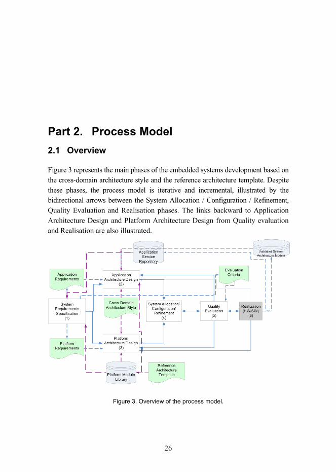
Figure 3 represents the main phases of the embedded systems development based on the cross-domain architecture style and the reference architecture template. Despite these phases, the process model is iterative and incremental, illustrated by the bidirectional arrows between the System Allocation / Configuration / Refinement, Quality Evaluation and Realisation phases. The links backward to Application Architecture Design and Platform Architecture Design from Quality evaluation and Realisation are also illustrated.
Figure 3. Overview of the process model.
Part 2. Process Model
27
System engineering starts with the requirements specification phase, which results in the definition of the functional properties, non-functional properties, quality requirements and constraints of a system. The evaluation criteria are derived from the defined quality requirements and prioritized according to the scope and importance of the requirements. Evaluation criteria define goals for quality evaluation. Scoping helps in classifying the requirements into two categories: application specific and platform specific requirements, which form the input for application architecture design and platform architecture design.
The application architecture design phase follows the principles defined by the cross-domain architecture style and takes into account the existing services available at the application service repository and the platform module library. Application architecture design results in a platform independent model (PIM) of the application architecture.
Platform architecture design is done according to the cross-domain architecture style and the reference architecture template. The reference architecture template defines the structure and behaviour of the platform core services, classified according to the integration levels they belong to. The cross-domain style defines three integration levels: chip (Level 1), device (Level 2) and (open/closed) system (Level 3). The module library provide core and optional services at two abstraction levels: model level and code level (if the realization is available). If a particular service is missing from the platform module library, a new optional service is defined at the PSM (Platform Specific Model) level. The platform architecture design phase outputs an instance of the PIM (Platform Independent Model) at a specific integration level. That instance is further used as a system-platform model upon which the application-PIM is transformed and allocated.
The system allocation / configuration / refinement phase associates/maps the application architecture design model onto the platform architecture design model resulting in the system architecture model, which consists of a set of views: structure, behaviour, and allocation (deployment), which are required for the next phase; quality evaluation. In the system architecture design phase, the platform architecture is configured for the use of a specific platform. In fact, in this phase, the whole system architecture is the first time described as a whole, and therefore, several refinements are typically needed. These refinements may be required before and after performing the quality evaluation phase. Architecture modelling and evaluation is a highly iterative and incremental process, and which steps need to be performed depends on the improvements defined as the results of quality evaluation.

Part 2. Process Model
28
Depending on the evaluation methods used, specific models may be needed for quality evaluation purposes. Thus, the diagrams of the defined views are transformed horizontally for the specific case at hand.
The evaluation process is iterative; it starts from the quality requirements of the highest priority and concludes with the quality properties of low priority. Each quality property is evaluated separately, and thereafter a tradeoffs analysis is conducted. If conflicts are encountered, a new iteration is taken (i.e. System Allocation / Configuration / Refinement and Quality Evaluation phases). When quality requirements are met, the realization of the system is made by manufacturing hardware and implementing software. Realization includes a set of refinement and testing phases, which are not discussed here. The assumption is that after unit, integration and validation tests, a new application and an optional (domain-specific) service are accepted. Thereafter, the new application can be included in the application service repository as a new reusable service and the validated architecture in the repository of validated system architecture models. The focus is on how to develop applications on top of platforms that follow the principles defined by the cross-domain style and reference architecture template.
2.2 Process Phases
The process phases 1�6 in Figure 3 are here described in more detail. The description elements of each phase define the purpose, preconditions and results of each phase. Moreover, the approaches with appropriate modelling languages and tools are introduced whenever possible in spite of the limited space.
2.2.1 System Requirements Specification
Description The System Requirements Specification phase will produce the requirements documents for the development of applications and platforms of the cross-domain enabled embedded systems. This phase will also specify the evaluation criteriato be applied in the Quality Evaluation phase.
Start conditions The decision to develop a new cross-domain architecture compliant product/system.
Triggers Application architecture design and platform architecturedesign phases.
Part 2. Process Model
29
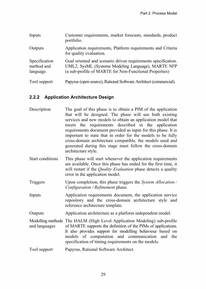
Inputs Customer requirements, market forecasts, standards, productportfolio.
Outputs Application requirements, Platform requirements and Criteriafor quality evaluation.
Specification method and language
Goal oriented and scenario driven requirements specification.UML2, SysML (Systems Modeling Language), MARTE NFP(a sub-profile of MARTE for Non-Functional Properties)
Tool support Papyrus (open source), Rational Software Architect (commercial).
2.2.2 Application Architecture Design
Description The goal of this phase is to obtain a PIM of the applicationthat will be designed. The phase will use both existing services and new models to obtain an application model thatmeets the requirements described in the applicationrequirements document provided as input for this phase. It isimportant to state that in order for the models to be fully cross-domain architecture compatible, the models used andgenerated during this stage must follow the cross-domain architecture style.
Start conditions This phase will start whenever the application requirementsare available. Once this phase has ended for the first time, it will restart if the Quality Evaluation phase detects a quality error in the application model.
Triggers Upon completion, this phase triggers the System Allocation / Configuration / Refinement phase.
Inputs Application requirements document, the application service repository and the cross-domain architecture style and reference architecture template.
Outputs Application architecture as a platform independent model.
Modelling methods and languages
The HALM (High Level Application Modeling) sub-profile of MARTE supports the definition of the PIMs of applications. It also provides support for modelling behaviour based on models of computation and communication and thespecification of timing requirements on the models.
Tool support Papyrus, Rational Software Architect.
Part 2. Process Model
30
2.2.3 Platform Architecture Design
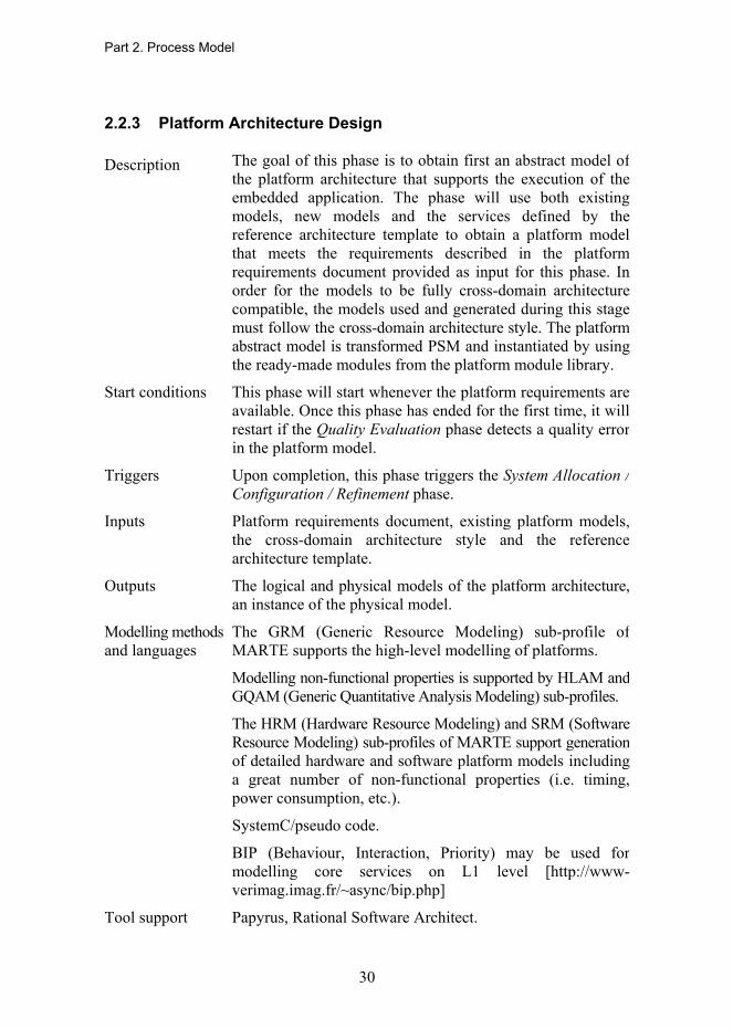
Description The goal of this phase is to obtain first an abstract model ofthe platform architecture that supports the execution of theembedded application. The phase will use both existing models, new models and the services defined by thereference architecture template to obtain a platform modelthat meets the requirements described in the platformrequirements document provided as input for this phase. Inorder for the models to be fully cross-domain architecture compatible, the models used and generated during this stagemust follow the cross-domain architecture style. The platform abstract model is transformed PSM and instantiated by using the ready-made modules from the platform module library.
Start conditions This phase will start whenever the platform requirements areavailable. Once this phase has ended for the first time, it willrestart if the Quality Evaluation phase detects a quality error in the platform model.
Triggers Upon completion, this phase triggers the System Allocation / Configuration / Refinement phase.
Inputs Platform requirements document, existing platform models,the cross-domain architecture style and the reference architecture template.
Outputs The logical and physical models of the platform architecture,an instance of the physical model.
Modelling methods and languages
The GRM (Generic Resource Modeling) sub-profile of MARTE supports the high-level modelling of platforms.
Modelling non-functional properties is supported by HLAM and GQAM (Generic Quantitative Analysis Modeling) sub-profiles.
The HRM (Hardware Resource Modeling) and SRM (SoftwareResource Modeling) sub-profiles of MARTE support generationof detailed hardware and software platform models including a great number of non-functional properties (i.e. timing, power consumption, etc.).
SystemC/pseudo code.
BIP (Behaviour, Interaction, Priority) may be used formodelling core services on L1 level [http://www-verimag.imag.fr/~async/bip.php]
Tool support Papyrus, Rational Software Architect.
Part 2. Process Model
31
2.2.4 System Allocation / Configuration / Refinement
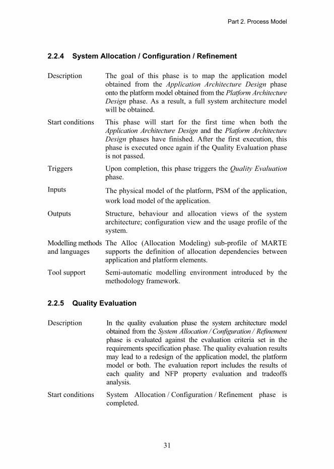
Description The goal of this phase is to map the application modelobtained from the Application Architecture Design phaseonto the platform model obtained from the Platform ArchitectureDesign phase. As a result, a full system architecture modelwill be obtained.
Start conditions This phase will start for the first time when both theApplication Architecture Design and the Platform ArchitectureDesign phases have finished. After the first execution, thisphase is executed once again if the Quality Evaluation phaseis not passed.
Triggers Upon completion, this phase triggers the Quality Evaluationphase.
Inputs The physical model of the platform, PSM of the application,work load model of the application.
Outputs Structure, behaviour and allocation views of the systemarchitecture; configuration view and the usage profile of thesystem.
Modelling methods and languages
The Alloc (Allocation Modeling) sub-profile of MARTEsupports the definition of allocation dependencies betweenapplication and platform elements.
Tool support Semi-automatic modelling environment introduced by themethodology framework.
2.2.5 Quality Evaluation
Description In the quality evaluation phase the system architecture modelobtained from the System Allocation / Configuration / Refinementphase is evaluated against the evaluation criteria set in therequirements specification phase. The quality evaluation resultsmay lead to a redesign of the application model, the platformmodel or both. The evaluation report includes the results ofeach quality and NFP property evaluation and tradeoffsanalysis.
Start conditions System Allocation / Configuration / Refinement phase iscompleted.
Part 2. Process Model
32
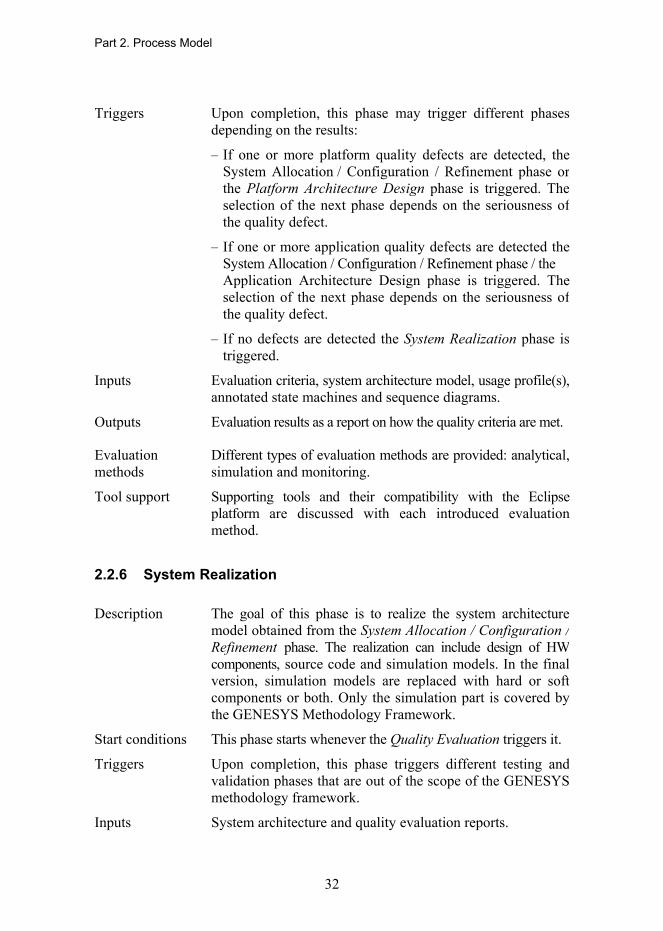
Triggers Upon completion, this phase may trigger different phasesdepending on the results:
� If one or more platform quality defects are detected, theSystem Allocation / Configuration / Refinement phase orthe Platform Architecture Design phase is triggered. Theselection of the next phase depends on the seriousness ofthe quality defect.
� If one or more application quality defects are detected theSystem Allocation / Configuration / Refinement phase / the Application Architecture Design phase is triggered. Theselection of the next phase depends on the seriousness ofthe quality defect.
� If no defects are detected the System Realization phase istriggered.
Inputs Evaluation criteria, system architecture model, usage profile(s),annotated state machines and sequence diagrams.
Outputs Evaluation results as a report on how the quality criteria are met.
Evaluation methods
Different types of evaluation methods are provided: analytical,simulation and monitoring.
Tool support Supporting tools and their compatibility with the Eclipseplatform are discussed with each introduced evaluationmethod.
2.2.6 System Realization
Description The goal of this phase is to realize the system architecturemodel obtained from the System Allocation / Configuration /Refinement phase. The realization can include design of HWcomponents, source code and simulation models. In the finalversion, simulation models are replaced with hard or softcomponents or both. Only the simulation part is covered bythe GENESYS Methodology Framework.
Start conditions This phase starts whenever the Quality Evaluation triggers it.
Triggers Upon completion, this phase triggers different testing andvalidation phases that are out of the scope of the GENESYSmethodology framework.
Inputs System architecture and quality evaluation reports.

Part 2. Process Model
33
Outputs HW and SW realizations as simulations and running systems.
Modelling support Model transformation from UML-MARTE to required simulationmodels.
Tool support Code generation for simulations / virtual prototyping, mappingsfrom PSM to physical HW.
2.3 Artefacts
Application requirements
Description This document contains the requirements that the application has to meet. It is the main input for the Application Architecture Design phase.
Produced by System Requirements Specification phase.
Used by Application Architecture Design phase.
Platform requirements
Description This document contains the requirements that have beendefined for the embedded platform. It is the main input forthe Platform Architecture Design phase.
Produced by System Requirements Specification phase.
Used by Platform Architecture Design phase.
Evaluation criteria
Description This document contains the criteria to be followed in thequality evaluation.
Produced by System Requirements Specification phase.
Used by Quality Evaluation phase.
Cross-domain architectural style
Description The cross-domain architectural style defines 24 principles that the application and platform architecture design phasesfollow.
Produced by GENESYS Architecture work package and Architecture Board.

Part 2. Process Model
34
Used by Application Architecture Design and Platform ArchitectureDesign phases.
Reference architecture template
Description The reference architecture template documents the core andoptional services as a service taxonomy which categorizes the service descriptions. The template also describes how thedefined services are adopted to different integration levels.
Produced by GENESYS WP1-WP2 (optional services) WP4-WP6 (core services).
Used by Platform Architecture Design phase.
Platform Module Library
Description A repository of existing platform modules (models orrealizations or both) that can be used such as for defining theplatform architecture.
Used by Platform Architecture Design phase.
Application Service Repository
Description A repository of existing application services that can be used as such for designing application architecture. Applications are defined as DASs which are distributed application systemscomposed of jobs.
Used by Application Architecture Design phase.

35
Part 3. Modelling and Evaluation 3.1 System Requirements Specification
The system requirements specification is the entry point to the development process (Figure 3). As requirements analysis and management is such a wide topic, while at the same time often being constrained by existing company or project specific process models, the methodology framework does not prescribe a detailed requirements process. Instead it describes a set of artefacts and activities which are useful or required for the later phases and in some places provides a choice between multiple options or optional activities.
The methodology framework categories requirements into three classes: application requirements, platform requirements and system requirements according the scope of a requirement (Figure 5). Requirements and constraints related to the demands of users and domains are more likely to influence the application architecture design, while technology related requirements will mostly affect the platform architecture design. System requirements and constraints have influence in the application architecture and the platform architecture.
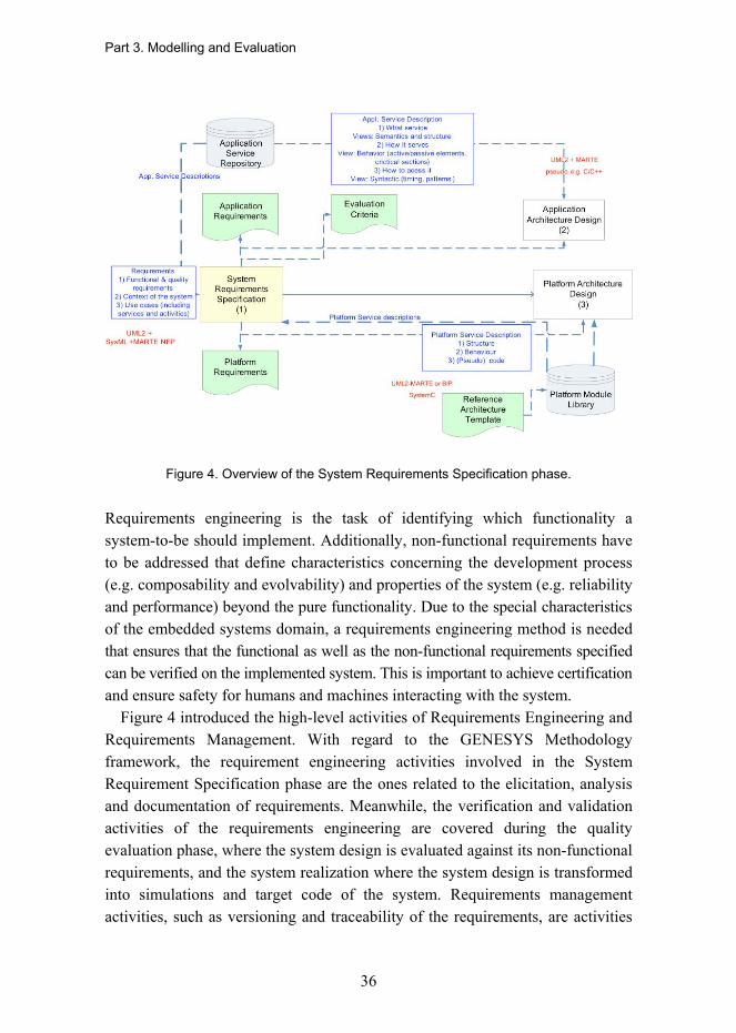
The System Requirements Specification phase (Figure 4) will produce the requirements documents for the development of applications and platforms of the cross-domain style enabled embedded systems. This phase will also specify the evaluation criteria to be applied in the Quality Evaluation phase.
Part 3. Modelling and Evaluation
36
Figure 4. Overview of the System Requirements Specification phase.
Requirements engineering is the task of identifying which functionality a system-to-be should implement. Additionally, non-functional requirements have to be addressed that define characteristics concerning the development process (e.g. composability and evolvability) and properties of the system (e.g. reliability and performance) beyond the pure functionality. Due to the special characteristics of the embedded systems domain, a requirements engineering method is needed that ensures that the functional as well as the non-functional requirements specified can be verified on the implemented system. This is important to achieve certification and ensure safety for humans and machines interacting with the system.
Figure 4 introduced the high-level activities of Requirements Engineering and Requirements Management. With regard to the GENESYS Methodology framework, the requirement engineering activities involved in the System Requirement Specification phase are the ones related to the elicitation, analysis and documentation of requirements. Meanwhile, the verification and validation activities of the requirements engineering are covered during the quality evaluation phase, where the system design is evaluated against its non-functional requirements, and the system realization where the system design is transformed into simulations and target code of the system. Requirements management activities, such as versioning and traceability of the requirements, are activities
Part 3. Modelling and Evaluation
37
transverse to all phases of the methodology; i.e. are not covered in specific phases but are handled all along the lifecycle.
3.1.1 Requirements Elicitation
The objective of this first activity is to build and understand the problem that the system-to-be is supposed to solve. Elicitation seeks to discover all potential sources of requirements including:
• Goals: high level objectives that the system needs to satisfy.
• Domain knowledge: is necessary in order to allow the requirement engineer to obtain specific knowledge not directly provided by the stakeholders.
• Stakeholders: provide different viewpoints with regard to the functionality that the system must provide.
• Operational environment: the system-to-be will be restricted by several factors, among them are, for example, the restrictions with regard to software or hardware where it should be deployed or the interfaces that it must provide in order to interact with legacy systems.
• Organizational environment: impact of the structure, culture and internal policies of the organizations involved needs to be assessed in determining requirements. Thus, there will be project and process related requirements caused, for example, by the need of following a certain project management standard like the V-Model XT or by the need for a certain certification, this is especially relevant to safety critical systems.
• Laws or regulations: usually the system is constrained by the fulfilment of specific constraints related to regulations or laws such as safety regulations, data protection laws and similar.
The most common techniques for capturing requirements are: interviews, questionnaires, scenarios, prototypes or facilitated meetings. Going in-depth into these techniques is out of the scope of this deliverable.
Part 3. Modelling and Evaluation
38
3.1.2 Requirements Analysis and Documentation
Regarding the requirement analysis and documentation activity the requirements are structured and prioritized. The result of this activity is a model of the business requirements, the application requirements, a model of the requirements and constraints for the platform and a set of quality criteria that will be used during the quality evaluation in order to validate the system architecture design.
This activity involves the following tasks:
• Classifying requirements: grouping requirements into logical entities. Different criteria can be used: priority, architecture/application, functional/ non-functional, associated risk, etc. In Figure 5, an example of the classification schema is provided in order to ease this clustering.
• Prioritizing requirements: establishing the relative importance and risk of each requirement and establishing an implementation priority.
• Conceptual modelling: abstraction behaviour and structure models of the system are designed in order to get an understanding of the problem and transfer this understanding to the developers involved in the system architecture design.
• Requirements negotiation: addresses problems within the requirements where conflicts occur between stakeholders� needs, between requirements and resources, or between system capabilities and constraints.

Part 3. Modelling and Evaluation
39
Figure 5. An example of classified attributes of requirements.
Regarding requirements documentation, each requirement will be described at least by the following fields:
• Id: a unique identifier
• Text: a textual description that describes the requirement
• Source: states the origin of this requirement. The following categories are considered: customer / operational environment / organizational environment / law / regulation.
• Kind (Functional/Non-Functional/Quality): states if the requirement is related to the fulfilment of a certain functional capability or if it is related to the fulfilment of a certain quantitative or qualitative constraint or quality attribute. An example of a constraint is a time deadline and an example of quality attribute performance, e.g. responsiveness of the system.
• Scope (Application/Platform/System): states if the requirement imposes a constraint on the application or on the architecture.

Part 3. Modelling and Evaluation
40
• Development phase: this information is used in order to trace the model elements from other artefacts during the development phase that contribute to satisfying the requirement.
• Status: this field will describe the current state of the requirement. There are four possible states for a requirement: feasible (the requirement has been considered valid by a requirements engineer or a checking engine), unfeasible (an opposite case), satisfied (it has already been satisfied) or undetermined (the requirement has not been analyzed yet).
• Risk: associated to this requirement
• Priority: assigned to this requirement.
The most important fields for quality requirements are: Id, Kind, Scope, and Priority. Moreover, the requirements of the execution qualities, e.g. reliability, need an attribute including the required, estimated, predicted and measured values.
In order to refine the requirements the goal-oriented requirement engineering approach is proposed together with the usage of a use case and scenario analysis. A goal expresses some objective to be achieved by the system. High level goals, such as business or user requirements, can be gradually refined into more concrete sub-goals by asking how the requirement is supposed to be fulfilled; thus, those sub-goals will contribute to the fulfilment of the higher level goal. This refinement process can be repeated until a suitable granularity is achieved. If the refinement and subdivision of requirements is performed correctly, it is sufficient for the system to fulfil those primitive requirements, as all other requirements are fulfilled by composition. This decomposition of requirements is represented usually by direct acyclic graphs, although in the methodology framework they are represented by SysML requirement diagrams by using the hierarchical relation that is established among requirements. Finally, the quality criteria are defined based on the non-functional and quality requirements and constraints.
Use cases are also used, especially in order to document application architecture requirements. A use case defines a system-level capability without revealing or implying any particular implementation or even design of that capability. Each use cases will be related to a certain amount of requirements. A use case has associated pre and post conditions that constrain its activation. Use cases describe the context where the system is used, including the system and
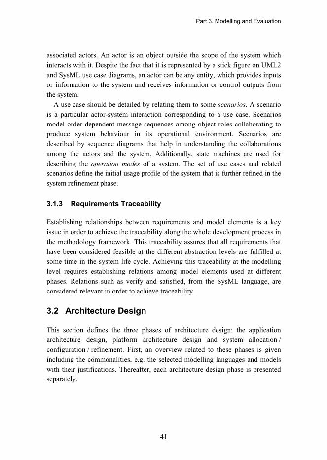
Part 3. Modelling and Evaluation
41
associated actors. An actor is an object outside the scope of the system which interacts with it. Despite the fact that it is represented by a stick figure on UML2 and SysML use case diagrams, an actor can be any entity, which provides inputs or information to the system and receives information or control outputs from the system.
A use case should be detailed by relating them to some scenarios. A scenario is a particular actor-system interaction corresponding to a use case. Scenarios model order-dependent message sequences among object roles collaborating to produce system behaviour in its operational environment. Scenarios are described by sequence diagrams that help in understanding the collaborations among the actors and the system. Additionally, state machines are used for describing the operation modes of a system. The set of use cases and related scenarios define the initial usage profile of the system that is further refined in the system refinement phase.
3.1.3 Requirements Traceability
Establishing relationships between requirements and model elements is a key issue in order to achieve the traceability along the whole development process in the methodology framework. This traceability assures that all requirements that have been considered feasible at the different abstraction levels are fulfilled at some time in the system life cycle. Achieving this traceability at the modelling level requires establishing relations among model elements used at different phases. Relations such as verify and satisfied, from the SysML language, are considered relevant in order to achieve traceability.
3.2 Architecture Design
This section defines the three phases of architecture design: the application architecture design, platform architecture design and system allocation / configuration / refinement. First, an overview related to these phases is given including the commonalities, e.g. the selected modelling languages and models with their justifications. Thereafter, each architecture design phase is presented separately.

Part 3. Modelling and Evaluation
42
3.2.1 Selection of Modelling Languages
The architectural descriptions, which are outcome of the phases of application architecture design, platform architecture design and system allocation / configuration / refinement, are combinations of textual and graphical descriptions. English is used for textual descriptions. Graphical models are described by the selected set of languages defined in Figure 16.
Figure 16. Architecture design phases and the selected modelling languages.
The service interface descriptions have to define the following information: syntax for accessing a service, service semantics (i.e. the goal of a service) and behaviour of a service (i.e. how the purpose of the service is achieved).
The four description languages, i.e. UML2 MARTE profile, Web Service Description Language (WSDL), the BIP-model (Verimag) and SystemC, were evaluated by applying them to describing two applications, i.e. a multimedia application and a cruise control system. The comparison of service description languages is introduced in Table 2. The comparison factors have been derived from the requirements of the methodology framework.
Service properties were to be described from syntax, semantic and quality points of view. Service semantic descriptions were especially required in open
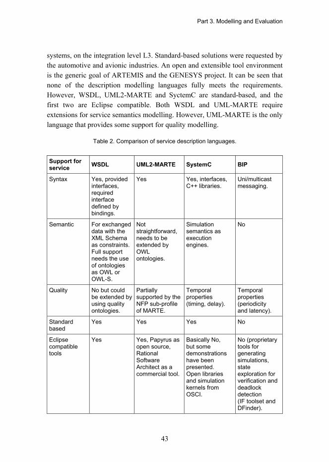
Part 3. Modelling and Evaluation
43
systems, on the integration level L3. Standard-based solutions were requested by the automotive and avionic industries. An open and extensible tool environment is the generic goal of ARTEMIS and the GENESYS project. It can be seen that none of the description modelling languages fully meets the requirements. However, WSDL, UML2-MARTE and SyctemC are standard-based, and the first two are Eclipse compatible. Both WSDL and UML-MARTE require extensions for service semantics modelling. However, UML-MARTE is the only language that provides some support for quality modelling.
Table 2. Comparison of service description languages.
Support for service WSDL UML2-MARTE SystemC BIP
Syntax Yes, provided interfaces, required interface defined by bindings.
Yes Yes, interfaces, C++ libraries.
Uni/multicast messaging.
Semantic For exchanged data with the XML Schema as constraints. Full support needs the use of ontologies as OWL or OWL-S.
Not straightforward, needs to be extended by OWL ontologies.
Simulation semantics as execution engines.
No
Quality No but could be extended by using quality ontologies.
Partially supported by the NFP sub-profile of MARTE.
Temporal properties (timing, delay).
Temporal properties (periodicity and latency).
Standard based
Yes Yes Yes No
Eclipse compatible tools
Yes Yes, Papyrus as open source, Rational Software Architect as a commercial tool.
Basically No, but some demonstrations have been presented. Open libraries and simulation kernels from OSCI.
No (proprietary tools for generating simulations, state exploration for verification and deadlock detection (IF toolset and DFinder).
Part 3. Modelling and Evaluation
44
As a conclusion, the UML-MARTE was selected for a common modelling language. Moreover, SystemC is needed for platform architecture design. BIP is applied to L1 level core services.
Because service semantic descriptions are needed in open systems on the level L3, two ontology languages were compared: Web Service Modelling Ontology (WSMO) and the Web Ontology Language for Services OWL-S [Feier 2005, Fensel 2007, OWL 2008]. The purpose of OWL-S is to define a set of basic classes and properties for describing services so that users and software agents are able to automatically discover, invoke, compose and monitor Web resources offering services. OWL-S supports service descriptions in a wide sense and does not focus on any particular application domain. WSMO aims to create an ontology for describing various aspects related to Semantic Web Services and therefore it focuses on ontology integration and providing support for specific application domains (e.g. e-Commerce and e-Work).
OWL-S doesn�t explicitly delimit what principles are applied to the development of the ontology. WSMO is more explicit; it is grounded on a number of principles of the domain that the ontology formally represents. Moreover, WSMO is based on the conceptual work done in WSMF (the framework that served as a starting point for WSMO) and thus it is a conceptually more focused approach than OWL-S. Comparison of the OWL-S and WSMO is presented Table 3. The comparison factors intend to illustrate the advantages and shortcomings of two ontology oriented approaches; the general purpose OWL-S and the specific purpose WSMO. As seen, WSMO is focused but extensible, whereas OWL-S is not limited to any application domain, but its adoption to new domains might be laborious because of limited capabilities and their extensibility.
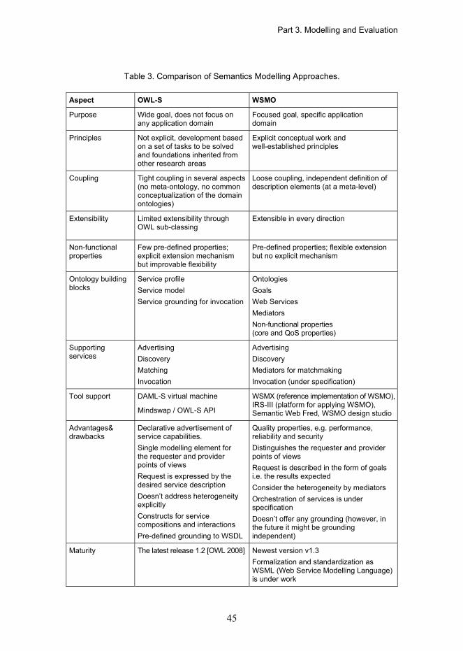
Part 3. Modelling and Evaluation
45
Table 3. Comparison of Semantics Modelling Approaches.
Aspect OWL-S WSMO
Purpose Wide goal, does not focus on any application domain
Focused goal, specific application domain
Principles Not explicit, development based on a set of tasks to be solved and foundations inherited from other research areas
Explicit conceptual work and well-established principles
Coupling Tight coupling in several aspects (no meta-ontology, no common conceptualization of the domain ontologies)
Loose coupling, independent definition of description elements (at a meta-level)
Extensibility Limited extensibility through OWL sub-classing
Extensible in every direction
Non-functional properties
Few pre-defined properties; explicit extension mechanism but improvable flexibility
Pre-defined properties; flexible extension but no explicit mechanism
Ontology building blocks
Service profile Service model Service grounding for invocation
Ontologies Goals Web Services Mediators Non-functional properties (core and QoS properties)
Supporting services
Advertising Discovery Matching Invocation
Advertising Discovery Mediators for matchmaking Invocation (under specification)
Tool support DAML-S virtual machine
Mindswap / OWL-S API
WSMX (reference implementation of WSMO), IRS-III (platform for applying WSMO), Semantic Web Fred, WSMO design studio
Advantages& drawbacks
Declarative advertisement of service capabilities. Single modelling element for the requester and provider points of views Request is expressed by the desired service description Doesn�t address heterogeneity explicitly Constructs for service compositions and interactions Pre-defined grounding to WSDL
Quality properties, e.g. performance, reliability and security Distinguishes the requester and provider points of views Request is described in the form of goals i.e. the results expected Consider the heterogeneity by mediators Orchestration of services is under specification Doesn�t offer any grounding (however, in the future it might be grounding independent)
Maturity The latest release 1.2 [OWL 2008] Newest version v1.3 Formalization and standardization as WSML (Web Service Modelling Language) is under work

Part 3. Modelling and Evaluation
46
Because the use of any ontology language for describing service semantics is not straightforward, their application was not appropriate due to our tight schedule. Therefore, further studies on service semantic modelling were transferred into future ARTEMIS projects.
The following sub-profiles of MARTE are applied to architecture modelling:
Sub-profile What for to be used
NFP � Non-Functional Properties For defining non-functional and quality properties
HLAM � High Level Application Modelling
For application architecture modelling
GCM � Generic Component Model For defining the structure of applications
GRM � Generic Resource Modelling For platform architecture modelling
Alloc � Allocation Modelling For allocating applications to platform services
SRM � Software Resources Modelling
For modelling operating systems, concurrency and interactions of applications.
HRM � Hardware resources modelling
For detailed hardware modelling
GQAM � Generic Analysis Modelling
Platform modelling for analysis.
3.2.2 Architectural Elements
Platform services are described at the PIM level. The platform modules are described at the PSM level. The GENESYS template defines a taxonomy of platform services; a set of core and optional services classified into categories according to the integration levels (L1 (chip level), L2 (device level), and L3 (system level)), functionality, dependability and security. The platform modules are described in the platform module library. The platform modules are used for describing the execution platform, upon which the applications (DASs) composed of jobs (i.e. an ordered set of services) are mapped. There are three types of components named according to the integration levels they are used: IP-Core, Chip and Device. Each type of component has four types of interface:

Part 3. Modelling and Evaluation
47
• LIF (Linking Interface) � for communication between applications (DASs and jobs) on the same integration level.
• DM (Diagnostics and maintenance) � for monitoring platform execution on the same integration level.
• CP (Configuration and planning) � for controlling and configuring an execution platform.
• LI (Local interface) � connecting the integration level to the environment and the gateway component, through which the component is connected to the next integration level.
3.2.3 Architectural Views, Models and Transformations
Figure 7 gives an overview of the required architectural descriptions; application service description, platform service description, system architecture description and micro architectures.
The two last mentioned descriptions are based on the application and platform service descriptions but include some extra views or models required for completing the architectural description of that specific phase. Because quality evaluation is the next phase after architecture design, it has a strong influence on which views and models are required. Typically, structure, behaviour and allocation views are necessary for quality evaluation. Structure can be presented at different abstraction levels; for example, an application service can be modelled as a distributed application sub-system (DAS) composed of a set of jobs or as a job, and therefore, the structural view includes two models; one for defining the structure of DAS and one for defining the structure of involved jobs. They both belongs to the structural view but can be modelled by using the different constructs of the modelling language. Moreover, design information of interfaces is required for evaluating composability and evolvability of the system architecture. If the specific information required for quality evaluation is not available, the architectural models are to be transferred into another model that is suitable for the evaluation purposes at hand.
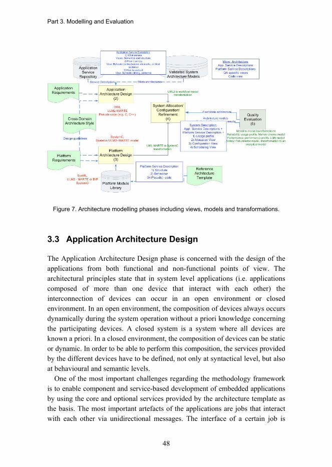
Part 3. Modelling and Evaluation
48
Figure 7. Architecture modelling phases including views, models and transformations.
3.3 Application Architecture Design
The Application Architecture Design phase is concerned with the design of the applications from both functional and non-functional points of view. The architectural principles state that in system level applications (i.e. applications composed of more than one device that interact with each other) the interconnection of devices can occur in an open environment or closed environment. In an open environment, the composition of devices always occurs dynamically during the system operation without a priori knowledge concerning the participating devices. A closed system is a system where all devices are known a priori. In a closed environment, the composition of devices can be static or dynamic. In order to be able to perform this composition, the services provided by the different devices have to be defined, not only at syntactical level, but also at behavioural and semantic levels.
One of the most important challenges regarding the methodology framework is to enable component and service-based development of embedded applications by using the core and optional services provided by the architecture template as the basis. The most important artefacts of the applications are jobs that interact with each other via unidirectional messages. The interface of a certain job is

Part 3. Modelling and Evaluation
49
composed by the definition of those messages. In order to be able to perform this composition, the services provided by the different jobs have to be defined, not only from a syntactical point of view, but also from behavioural and semantic points of view.
It is also possible that a service has constraints related to its versioning. Thus, the semantic view is used to give additional information about the meaning of the service. This information provides a means for distinguishing one service from another that provides a similar kind of functionality but at a different quality level or with different constraints. The semantic view is especially needed in open systems, where service bindings are performed at run-time. However, a similar type of information might be also needed in other integration levels in the future.
Since the semantic view is coupled with service properties provided through the service interfaces, it is common to find that the semantic view is mixed with the structural and syntactical views, therefore being modelled in the same diagrams, yet using different elements for each of the views.
In order to provide developers with models that are expressive enough, it is important to present the structures of the services and jobs in application architecture. The next sub-sections will cover the modelling of each of these views using UML2 and the MARTE profile. MARTE is a UML2 profile and, therefore, it cannot be used without it. It is important to note that UML provides several ways to describe the same aspects of the system models. This fact makes it difficult to provide a unique method to create the models as many different diagrams can be used to specify the same aspects in the models. For example, in many cases, state machines and activity diagrams can address the same behaviour.
The goal of the Application Architecture Design phase is to produce a platform independent model of an embedded application or applications. The phase produces the following views:
Structural view. The structural view contains the definition of DAS (i.e. interaction between jobs), the jobs (encapsulated pieces of application functionality), LIFs and messages that take part in the application under design.
Syntactical view. The syntactical view contains the description of the protocols that manage the access to a certain service. (The interface description is partly defined by the structural view and the syntactical view).

Part 3. Modelling and Evaluation
50
Behaviour view. The behaviour view defines the behaviour of the application at two levels: as behaviour of the application and as behaviour of the jobs involved in the application.
Semantic view. The semantic view provides information regarding the semantics of the application service. The semantic view is related to a service ontology that will be an enabler for service composition engines.
It is possible that many diagrams are included in a single view. It is also possible to describe two or more views in the same diagram but it is against the separation of concerns; one of the architecture design laws and breaching that law will lead to serious problems in architecture evolution.
In the next sections, each view is introduced by using the UML-MARTE modelling language. Service semantics can also be described with OWL and used through the UML-MARTE language. However, this means additional tool support from the interactive development environment. An example of combining OWL models with UML models is given in [Niemelä 2008].
3.3.1 Structural View
The structural view describes the application as a whole and the building blocks, i.e. jobs and interfaces, of which it is combined. A job is a) a constituting element of a DAS, b) forms the basic unit of work, and c) interacts with other jobs through the exchange of messages in order to work towards a common goal to provide the application services. The structural view of an application provides information regarding the construction of the service. Services are defined by their interfaces. Therefore, the structural view is described as follows:
• Describe the jobs involved in the application under design.
• Describe the service interfaces of each job and messages passed through each interface.
• Describe the application as a composite of jobs (i.e. distributed application subsystem, DAS). Reuse the available application service descriptions.
• Describe the resources (e.g. variables, communication channel, etc.) shared between jobs.

Part 3. Modelling and Evaluation
51
• Map non-functional and quality requirements and constraints defined for the application in the system specification phase to the appropriate diagrams of the application.
The structural view has to describe the applications in terms of jobs, i.e. different tasks that must be executed. Moreover, the different services involved in the application must be defined in terms of their interfaces and the kind of messages they request/provide. Lastly, structural descriptions also include passive elements that help different jobs to communicate. The MARTE profile provides two specific sub-profiles for this kind of view:
• High-Level Application Modelling (HLAM) sub-profile and • Generic Component Model (GCM) sub-profile.
These two sub-profiles along with the UML2 constructs allow a rich description of applications and services.
The cruise control system (CCS) is used as an example to illustrate the structural view. The controller receives two input messages containing the current speed of a car and the desired speed value selected by a car driver and computes an output signal that affects the engine of the car. Thus, the controller provides three interfaces: two input interfaces each of which reads a speed signal, and an output interface which provides the control signal for the engine actuator. To model this controller we will use a UML active class stereotyped with <<RtUnit>> from the MARTE HLAM sub-profile (Table 4). The stereotype gives a class for the semantics of a task or a set of tasks that will be executed in some computing resource of the underlying platform. The stereotype includes many properties that may increase expressivity in a class. A complete list of the <<RtUnit>> parameters is provided in Table 4.
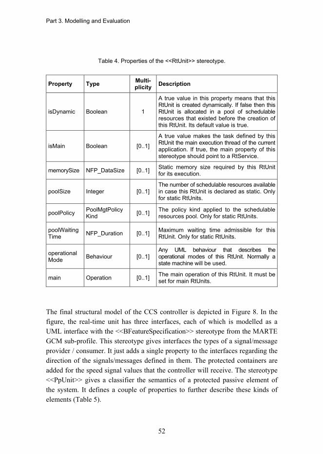
Part 3. Modelling and Evaluation
52
Table 4. Properties of the <<RtUnit>> stereotype.
Property Type Multi-plicity Description
isDynamic Boolean 1
A true value in this property means that this RtUnit is created dynamically. If false then this RtUnit is allocated in a pool of schedulable resources that existed before the creation of this RtUnit. Its default value is true.
isMain Boolean [0..1]
A true value makes the task defined by this RtUnit the main execution thread of the current application. If true, the main property of this stereotype should point to a RtService.
memorySize NFP_DataSize [0..1] Static memory size required by this RtUnit for its execution.
poolSize Integer [0..1] The number of schedulable resources available in case this RtUnit is declared as static. Only for static RtUnits.
poolPolicy PoolMgtPolicy Kind [0..1] The policy kind applied to the schedulable
resources pool. Only for static RtUnits.
poolWaitingTime NFP_Duration [0..1] Maximum waiting time admissible for this
RtUnit. Only for static RtUnits.
operational Mode Behaviour [0..1]
Any UML behaviour that describes the operational modes of this RtUnit. Normally a state machine will be used.
main Operation [0..1] The main operation of this RtUnit. It must be set for main RtUnits.
The final structural model of the CCS controller is depicted in Figure 8. In the figure, the real-time unit has three interfaces, each of which is modelled as a UML interface with the <<BFeatureSpecification>> stereotype from the MARTE GCM sub-profile. This stereotype gives interfaces the types of a signal/message provider / consumer. It just adds a single property to the interfaces regarding the direction of the signals/messages defined in them. The protected containers are added for the speed signal values that the controller will receive. The stereotype <<PpUnit>> gives a classifier the semantics of a protected passive element of the system. It defines a couple of properties to further describe these kinds of elements (Table 5).
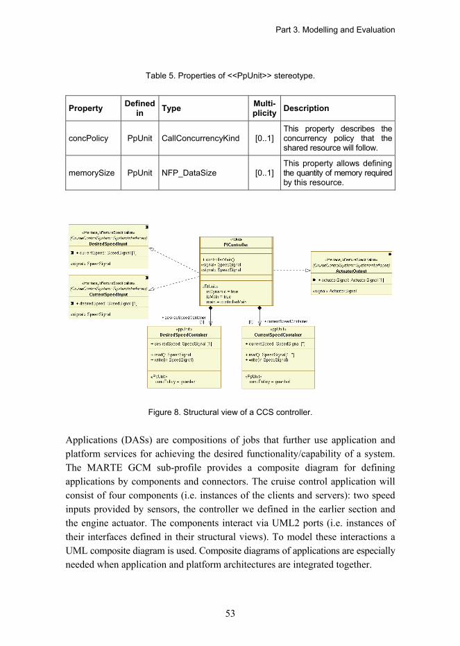
Part 3. Modelling and Evaluation
53
Table 5. Properties of <<PpUnit>> stereotype.
Property Defined in Type Multi-
plicity Description
concPolicy PpUnit CallConcurrencyKind [0..1] This property describes the concurrency policy that the shared resource will follow.
memorySize PpUnit NFP_DataSize [0..1] This property allows defining the quantity of memory required by this resource.
Figure 8. Structural view of a CCS controller.
Applications (DASs) are compositions of jobs that further use application and platform services for achieving the desired functionality/capability of a system. The MARTE GCM sub-profile provides a composite diagram for defining applications by components and connectors. The cruise control application will consist of four components (i.e. instances of the clients and servers): two speed inputs provided by sensors, the controller we defined in the earlier section and the engine actuator. The components interact via UML2 ports (i.e. instances of their interfaces defined in their structural views). To model these interactions a UML composite diagram is used. Composite diagrams of applications are especially needed when application and platform architectures are integrated together.

Part 3. Modelling and Evaluation
54
Figure 9. The cruise control system composite.
Figure 9 shows the cruise control system using UML2 and MARTE. The ports have been stereotyped with <<MessagePort>> stereotypes from GCM sub-profile that give the ports the semantics of being message-based communications. The CGM sub-profile also allows modelling data streams. In order to do so, we would use the <<FlowPort>> stereotype instead (Table 6).
Table 6. Properties of the <<MessagePort>> and <<FlowPort>>.
Property Type Multiplicity Description
isAtomic Boolean 1
If true the port cannot provide/require services, it just produces/consumes signals. Additionally, an atomic port�s direction is defined by its specification interface.
isConjugated Boolean 1 Only for non-atomic ports. If true all the directions of the FlowProperty elements are reverted.
direction DirectionKind[0..1] [0..1] Only for non-atomic ports. It specifies the direction of the port.

Part 3. Modelling and Evaluation
55
3.3.2 Syntactical View
The syntactical view of the application describes how the services are accessed. A syntactical description includes:
• a description of the messages involved in the access of a certain service,
• a description of the communication protocols used,
• the operational modes of the applications (e.g. different QoS, emergency modes, etc.), and
• non-functional and quality properties related to message, communication protocols and operational modes.
The syntactical view of a service is often mixed with its structural view since service syntaxes are always related to structural elements. For example, messages are related to service interfaces and operational modes are related to the jobs that execute the service.
In order for clients to be able to access services it is mandatory that the service-users are aware of the syntax the services understand. In these kinds of applications, the syntax of a service is defined by the signals/messages that are exchanged by service-users and services and by the order in which these signals and messages are sent from service-users to services and vice versa.
To show an example of modelling the syntax of a service we will use the example of an application server. The structure of this server is depicted in Figure 10. As depicted in the figure, the server admits three different kinds of messages: a StartConnection message, a Data message and a CloseConnection message. The server also uses two messages to answer the clients: Ack and Nack. The protocol is defined using a UML2 state machine diagram that is pointed by the �operationalMode� property of the <<RtUnit>> stereotype (Figure 11). We also add a property to the server in other to keep track of its current state.

Part 3. Modelling and Evaluation
56
Figure 10. Structure of an application server.
Figure 11. State machine diagram of the application server protocol.
From a syntactical point of view, clients have to be aware of the structure of the messages they must send to the server in order to interact with it. Messages, as already has been shown, are modelled using UML2 signal elements. Figure 12 shows the messages involved in the current example.
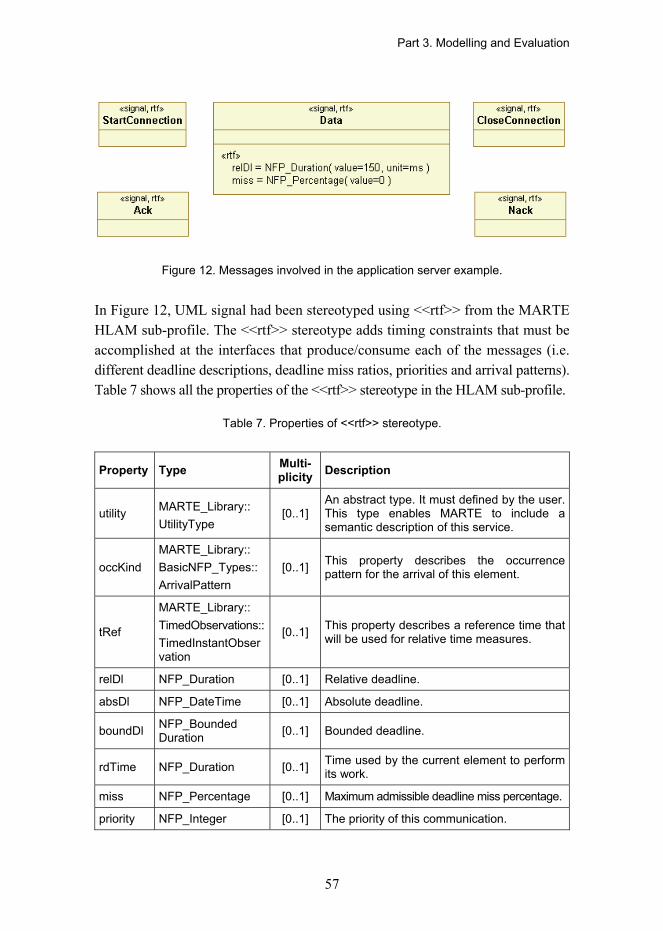
Part 3. Modelling and Evaluation
57
Figure 12. Messages involved in the application server example.
In Figure 12, UML signal had been stereotyped using <<rtf>> from the MARTE HLAM sub-profile. The <<rtf>> stereotype adds timing constraints that must be accomplished at the interfaces that produce/consume each of the messages (i.e. different deadline descriptions, deadline miss ratios, priorities and arrival patterns). Table 7 shows all the properties of the <<rtf>> stereotype in the HLAM sub-profile.
Table 7. Properties of <<rtf>> stereotype.
Property Type Multi-plicity Description
utility MARTE_Library:: UtilityType
[0..1] An abstract type. It must defined by the user. This type enables MARTE to include a semantic description of this service.
occKind MARTE_Library:: BasicNFP_Types:: ArrivalPattern
[0..1] This property describes the occurrence pattern for the arrival of this element.
tRef
MARTE_Library:: TimedObservations::TimedInstantObservation
[0..1] This property describes a reference time that will be used for relative time measures.
relDl NFP_Duration [0..1] Relative deadline.
absDl NFP_DateTime [0..1] Absolute deadline.
boundDl NFP_Bounded Duration [0..1] Bounded deadline.
rdTime NFP_Duration [0..1] Time used by the current element to perform its work.
miss NFP_Percentage [0..1] Maximum admissible deadline miss percentage.
priority NFP_Integer [0..1] The priority of this communication.
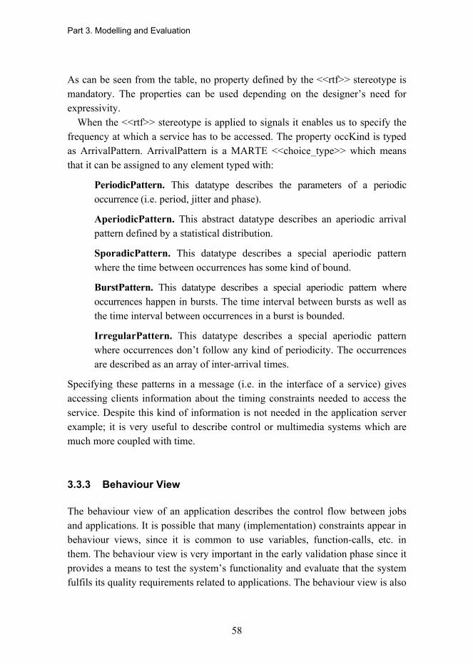
Part 3. Modelling and Evaluation
58
As can be seen from the table, no property defined by the <<rtf>> stereotype is mandatory. The properties can be used depending on the designer�s need for expressivity.
When the <<rtf>> stereotype is applied to signals it enables us to specify the frequency at which a service has to be accessed. The property occKind is typed as ArrivalPattern. ArrivalPattern is a MARTE <<choice_type>> which means that it can be assigned to any element typed with:
PeriodicPattern. This datatype describes the parameters of a periodic occurrence (i.e. period, jitter and phase).
AperiodicPattern. This abstract datatype describes an aperiodic arrival pattern defined by a statistical distribution.
SporadicPattern. This datatype describes a special aperiodic pattern where the time between occurrences has some kind of bound.
BurstPattern. This datatype describes a special aperiodic pattern where occurrences happen in bursts. The time interval between bursts as well as the time interval between occurrences in a burst is bounded.
IrregularPattern. This datatype describes a special aperiodic pattern where occurrences don�t follow any kind of periodicity. The occurrences are described as an array of inter-arrival times.
Specifying these patterns in a message (i.e. in the interface of a service) gives accessing clients information about the timing constraints needed to access the service. Despite this kind of information is not needed in the application server example; it is very useful to describe control or multimedia systems which are much more coupled with time.
3.3.3 Behaviour View
The behaviour view of an application describes the control flow between jobs and applications. It is possible that many (implementation) constraints appear in behaviour views, since it is common to use variables, function-calls, etc. in them. The behaviour view is very important in the early validation phase since it provides a means to test the system�s functionality and evaluate that the system fulfils its quality requirements related to applications. The behaviour view is also

Part 3. Modelling and Evaluation
59
crucial in the system realization phase, since the behaviour described in this view is what the developers will implement in the final product.
The HLAM sub-profile of MARTE provides the designer with a series of stereotypes to make some behavioural aspects present when describing the services and applications. The behavioural aspects supported by the HLAM stereotypes include quality of service (QoS) specification and execution, and concurrency and a synchronization aspects description.
The operations which support the services inside RtUnits can be given information about their behaviour. The HLAM sub-profile provides designer of the <<RtService>> stereotype to model how the servers react to incoming invocations. The properties defined for this stereotype are defined in Table 8 and Figure 13 shows the way this stereotype is used in the application server example.
Table 8. Properties of <<RtService>> stereotype.
Property Type Multiplicity Description
concPolicy ConcurrencyKind [0..1] This property describes the concurrency kind for this particular service.
exeKind ExecutionKind [0..1] This property describes how this service will behave upon its invocation.
isAtomic Boolean 1 This property specifies if this service will be executed without being interrupted by other invocations.
synchKind SynchronizationKind [0..1] This property describes how this service is synchronized with the invoking client.
The RtService stereotype is applied to the signal receptions in the interfaces of the server RtUnit. In order to add a finer grain description of the behaviour of the RtUnits or their interfaces, it is necessary to use activity diagrams, sequence diagrams or state machine diagrams. Figure 13 shows the activity diagram of the main operation of the controller RtUnit of the CCS example. The diagram shows that the controller starts up the system and then enters an endless loop in which it only performs the control algorithm on the speed samples provided by the sensors and then it sends a message to the engine actuator through the actuator output interface.

Part 3. Modelling and Evaluation
60
Using the MARTE stereotypes in this kind of diagrams increases their expressivity, including extra information. The <<rtf>> stereotype, described before, adds timing information to the actions. On the other hand, the <<RtAction>> introduces information regarding signal sending and reception. The properties included in this stereotype are described in Table 9.
Figure 13. Activity diagram of the main operation of the cruise control system controller.
Table 9. Properties of <<RtAction>> stereotype.
Property Type Multi-plicity Description
synchKind SynchronizationKind [0..1] It describes the type of synchronism that suits this signal communication.
isAtomic Boolean 1 It defines whether the attention of this communication will be done atomically. It is false by default.
msgSize NFP_DataSize [0..1] This parameter describes the size of the messages (signals) that are used in this communication.

Part 3. Modelling and Evaluation
61
The <<RtBehaviour>> stereotype is used in behavioural UML diagrams modelling how an RtService behaves with regard to invocation queues. It can be used in any kind of UML behaviour diagrams (state machines, activities and interactions). Figure 14 shows the activity diagram of the current speed signal reception.
Figure 14. Current speed reception activity of the CCS controller.
The RtBehaviour stereotype is very useful to model services that prioritize some invocations from others regarding their real-time parameters and QoS. The complete list of the properties defined in <<RtBehaviour>> is described in Table 10.
Table 10. Properties of <<RtBehaviour<< stereotype.
Property Type Multi-plicity Description
queueSchedPolicy GRM_BasicTypes::
SchedPolicyKind [0..1] The scheduling policy that will be
applied to the message queue.
queueSize Integer [0..1] Maximum number of messages that can be stored in the queue of the current behaviour.
msgMaxSize NFP_DataSize [0..1] Maximum size of the messages stored in this queue.

Part 3. Modelling and Evaluation
62
3.3.4 Semantic View
The semantic view describes the meaning of the services used in application design. Semantic information is required for:
• Functionality provided by the service,
• Quality properties of the service,
• Meaning of information/data provided by the service,
• Usage constraints of the service, and
• Context of a service, if it functional or quality properties can change according to the context.
Although the MARTE profile has great expressivity to describe real-time embedded applications, it does not include immediate mechanisms to distinguish one service from another from a semantic point of view apart from the plain service name.
Semantic information is often very close to ontologies and taxonomies. In order to use MARTE to fully describe the services of the GENESYS architecture template, it is necessary to define an ontology of the services that an embedded application can request/provide at the different integration levels. Once the ontology is defined, MARTE can be extended or adapted to support the inclusion of this ontological information.
The <<rtf>> stereotype, defined in the HLAM sub-profile of MARTE, has been widely used throughout this document to describe the GENESYS applications and services. <<rtf>> includes a property called �utility� that may enable to add the semantics to service interfaces by specifying it in the <<rtf>> stereotypes applied to the signals.
The UtilityType is defined as an abstract type in MARTE so that it can be refined into user defined types. Figure 15 shows an example refinement of the MARTE UtilityType to a GENESYSUtilityType with extra semantic information.

Part 3. Modelling and Evaluation
63
Figure 15. Extending UtilityType to add semantic information to the service description.
3.4 Platform Architecture Design
The Platform Architecture Design phase deals with the modelling of the platform architecture that supports the applications designed during the Application Architecture Design phase. The platform architecture is logical architecture that is realized as hardware and software.
The platform architecture design is highly related to the system requirements specification phase, the application architecture design and the GENESYS style and reference architecture template. Platform requirements can be business requirements, system requirements and technical constraints. Business requirements scope the platform architecture design. System requirements define which kinds of properties are required from the platform; they can be technical features and/or

Part 3. Modelling and Evaluation
64
restrictions that affect the platform like pricing, weight, communications. Technical constraints are based on earlier decisions or standards the platform has to support.
The cross-domain architecture style defines three integration levels at which applications might be developed: System Level (L3), Device Level (L2) and Chip Level (L1). Each of these levels addresses different application description challenges through the use of modelling techniques.
Chip level applications focus on developing software/hardware systems that will be implemented on single chips (e.g., Multi-Processor System-on-Chips). The platform components at this integration level consist of computation, storage and communication resources that are either taken from IP (Intellectual Property) libraries or developed/acquired if they do not exist. Software consists typically of RTOSes (Real-Time Operating Systems), device drivers and middleware on top of which services and applications are designed at the chip level.
Device level applications focus on creating complete embedded devices. They make use of platforms that can, for example, be composed of a set of chip level platforms providing services to device level applications. Additional middleware and services may be used on top to facilitate an efficient interface to applications.
System level applications are composed of a set of distributed devices that interact with each other. At this integration level only software platforms may need to be considered since the devices composing the application already have their hardware/software architecture defined.
Despite their nature, hardware or software, platform elements have to be considered using two different points of view: a structural view and a behavioural view. Both views are defined at the logical level. The first view provides a designer with an understanding of which kinds of building blocks the platform is composed of, and which kinds of services are provided for the applications. The behaviour view describes how the defined building blocks of the platform structure work together and depend on each other. It also enables system simulation that allows early detection of design errors, increases the quality of the final system and reduces maintenance costs.
Platform architecture modelling produces models of the following views:
Structural view. The view describes the platform architecture from its structural point of view. The platform architecture model is composed of resources (both SW and HW) at various levels of granularity (e.g., processor, computing node, multiple interconnected computing nodes).

Part 3. Modelling and Evaluation
65
Resources provide services described by using the core and optional services provided by the GENESYS template and/or new services if proper platform services are not available.
Behaviour view. The behaviour view describes the behaviour of the services included in the platform structural view. Basically, the behavioural descriptions of the high-level services are taken from the platform module library that includes the descriptions of the core and optional services defined by the GENESYS template.
Code view. Platform services are described in more detail in the code view. In what manner and how a service is described depends on what that information is needed for.
The structural and behaviour views form a skeleton of the whole platform architecture and are used for allocating/mapping application models onto it. The structural and behaviour views are described with UML-MARTE. Defining non-functional and quality properties is also possible in these views. In case, the core service has been described with BIP, the BIP to UML-MARTE transformation is required. The code view is described with SystemC.
3.4.1 Structural View
The structural view of a system�s platform is meant to describe which elements compose the execution platform. The execution platforms are composed of hardware and software elements. The structural views represent real elements that have critical influence on the non-functional properties of a system. These non-functionalities have to be captured in the platform models in order to be able to achieve useful simulation and evaluation results in future phases of the embedded systems development process.
The structural view of a system�s platform provides information about the real elements of the execution environment intended for the application/service under construction. Those model elements refer to real resources in the final systems.
MARTE provides platform modellers with the Generic Resource Modelling (GRM) sub-profile which allows for the high level description of embedded platforms including both SW and HW in a generic way, without going into details of the actual platforms (i.e. which processor and/or operating system). In the following subsections we will try to describe how to use this sub-profile to model the resources of the embedded platforms.

Part 3. Modelling and Evaluation
66
3.4.1.1 MARTE GRM Concepts for Execution Platform Modelling
An embedded system platform model is composed of models of SW and HW elements and their interaction relationships. The GRM sub-profile gives concepts Resource, ResourceService, and their corresponding instances ResourceInstance and ResourceServiceExecution. Resources are used to model the execution platform from a structural point of view, while the resource services supply the behavioural point of view. A resource may be structurally described in terms of its internal resources � this is represented by the �ownerownedElement� association in Resource inherited from the ModelElement meta-class. For example, a processing resource may be refined as a processor connected to a memory through a bus.
ResourceAmount, representing a generic quantity of the "amount" provided by the resource. This may be mapped to any significant quantification of the resource, like memory units, utilization, power, etc.
As it occurs with classifiers, the execution platform may be represented as a hierarchical structure of resources.
Resource types:
• StorageResource • Timingresource • SynchResource • ComputingResource • ConcurrencyResource • Deviceresource • CommunicationResource: CommunicationEndPoint,
CommunicationMedia.
Scheduler is defined as a kind of ResourceBroker that brings access to its brokered ProcessingResource or resources following a certain scheduling policy.
SchedulableResource is defined as a kind of ConcurrencyResource with logical concurrency.
When the executionBehaviours of concurrencyResources need to access common protected resources, the underlying scheduling mechanisms are typically implemented using some form of synchronization resource, (semaphore, mutex, etc.) with a protecting protocol to avoid priority inversions.

Part 3. Modelling and Evaluation
67
ResourceUsage links resources with concrete demands of usage over them. A few concrete forms of usage are defined at this level of specification under the concept of UsageTypedAmount; those are aimed to represent the consumption or temporary usage of memory, the time taken from a CPU, the energy from a power supply and the number of bytes to be sent through a network.
Platform architecture model � structural view
When the modelling execution platform it is usually presented as a hierarchical layered model, e.g., a platform layer consisting of a set of (different) computing nodes linked with (internal) network communication, computing node (also called a processing node or sub-system) layer consisting of components and component layer, all layers containing appropriate software implementing system services.
Examples at the component layer are processing (e.g. programmable processors), storage (e.g. volatile memories) and interconnection (e.g. bus) elements as well as an OS/scheduler and device drivers. Their services are of a basic type, like read, write, etc. Examples of NFP property types include e.g., clock frequency, cycles-per-instruction, pipelining, read-latency, write-latency and burst-latency.
An example at the computing node layer is composed of bus, different processor types each with private memory, the OS and device drivers, shared memory, shared I/O component and a shared network interface component (to connect to network communication at the platform layer). A processing node is capable of providing generic multi-tasking (multi-processing, multi-threading) and device driver services and e.g. (part of) core and optional services. Examples of NFP property types include e.g. task processing time, service processing time, the number of task switches, the number of processor cycles used, communication latency/delay, etc.
An example at the platform layer is illustrated by instances of different types of computing nodes connected with (internal) network communication. In addition to (internal) network communication services, the platform layer may provide e.g. (part of) core and optional services that are produced through interaction of several computing nodes and their services. Examples of NFP property types are similar to the computing node layer, but now possibly aggregated if services span several computing nodes.
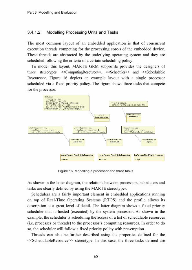
Part 3. Modelling and Evaluation
68
3.4.1.2 Modelling Processing Units and Tasks
The most common layout of an embedded application is that of concurrent execution threads competing for the processing core/s of the embedded device. These threads are abstracted by the underlying operating system and they are scheduled following the criteria of a certain scheduling policy.
To model this layout, MARTE GRM subprofile provides the designers of three stereotypes: <<ComputingResource>>, <<Scheduler>> and <<Schedulable Resource>>. Figure 16 depicts an example layout with a single processor scheduled via a fixed priority policy. The figure shows three tasks that compete for the processor.
Figure 16. Modelling a processor and three tasks.
As shown in the latter diagram, the relations between processors, schedulers and tasks are clearly defined by using the MARTE stereotypes.
Schedulers are a fairly important element in embedded applications running on top of Real-Time Operating Systems (RTOS) and the profile allows its description at a great level of detail. The latter diagram shows a fixed priority scheduler that is hosted (executed) by the system processor. As shown in the example, the scheduler is scheduling the access of a list of schedulable resources (i.e. processes or threads) to the processor�s computing resources. In order to do so, the scheduler will follow a fixed priority policy with pre-emption.
Threads can also be further described using the properties defined for the <<SchedulableResource>> stereotype. In this case, the three tasks defined are

Part 3. Modelling and Evaluation
69
described by �FixedPriorityParameters� instances which only contain one parameter: priority. The subprofile also defines parameter types for other scheduling policies. In order for the model to be consistent, it is necessary that the parameters used to describe system threads match the scheduling policy used by its scheduler.
3.4.1.3 Modelling Shared Resources
A problem related to multithread programming is handling access of the different tasks to the shared resources. MARTE GRM sub profile provides the users of two stereotypes to model shared resources depending on access protocols. These stereotypes are <<SynchronizationResource>> and <<MutualExclusionResource>>. The main difference between these two resources is that the synchronization resources refer to unmanaged elements like semaphores and mutexes while mutual exclusion resources refer to elements handled by an access protocol. Figure 17 shows the three tasks defined before and two shared resources of different types.
Figure 17. Modelling shared resources with MARTE.
The diagram shows how a shared variable can be modelled following both approaches. In this case the mutual exclusion resource depicted follows a priority
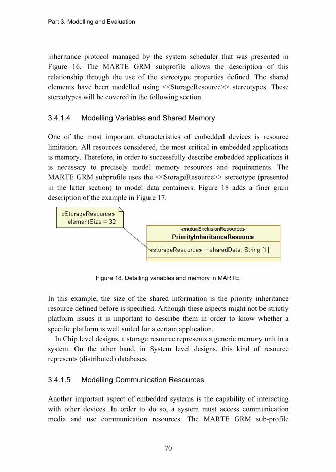
Part 3. Modelling and Evaluation
70
inheritance protocol managed by the system scheduler that was presented in Figure 16. The MARTE GRM subprofile allows the description of this relationship through the use of the stereotype properties defined. The shared elements have been modelled using <<StorageResource>> stereotypes. These stereotypes will be covered in the following section.
3.4.1.4 Modelling Variables and Shared Memory
One of the most important characteristics of embedded devices is resource limitation. All resources considered, the most critical in embedded applications is memory. Therefore, in order to successfully describe embedded applications it is necessary to precisely model memory resources and requirements. The MARTE GRM subprofile uses the <<StorageResource>> stereotype (presented in the latter section) to model data containers. Figure 18 adds a finer grain description of the example in Figure 17.
Figure 18. Detailing variables and memory in MARTE.
In this example, the size of the shared information is the priority inheritance resource defined before is specified. Although these aspects might not be strictly platform issues it is important to describe them in order to know whether a specific platform is well suited for a certain application.
In Chip level designs, a storage resource represents a generic memory unit in a system. On the other hand, in System level designs, this kind of resource represents (distributed) databases.
3.4.1.5 Modelling Communication Resources
Another important aspect of embedded systems is the capability of interacting with other devices. In order to do so, a system must access communication media and use communication resources. The MARTE GRM sub-profile

Part 3. Modelling and Evaluation
71
provides two stereotypes to model communication resources, both resources internal to the operating systems (i.e. pipes, IPC...) and network resources (i.e. Bluetooth, IP networks...). The following example depicts how a TCP socket connection is modelled using MARTE GRM.
Figure 19. Modelling communication resources in MARTE.
As shown in Figure 19, the <<CommunicationEndPoint>> stereotype is used to model the platform element in charge of transmitting the messages to a <<CommunicationMedia>> and/or receiving incoming messages from remote peers. Many real-time applications need predictable communication resources (e.g. industrial SCADA systems). These applications use real-time networks to achieve a predictable communication between network devices. MARTE provides support to model these kinds of networks. In the example a TCP/IP network is modelled. IP packets can be prioritized according to a fixed priority policy. In order to model this kind of behaviour, we have used a virtual network scheduler which is not related to a physical component, but yet affects the communication behaviour. Again, in order to keep the model consistency, the element sizes for communication media and end points must be the same/compatible.
The same stereotypes can be used in Chip level designs for modelling the communication buses and bus interfaces of the components.
3.4.1.6 Modelling Platform Black-boxes
It is common that embedded applications use both dedicated hardware and/or special software libraries to help developers perform a certain action (e.g. driver to access a sensor or an MP3 hardware coder). These pieces of hardware/software are treated as black boxed by the application designers and
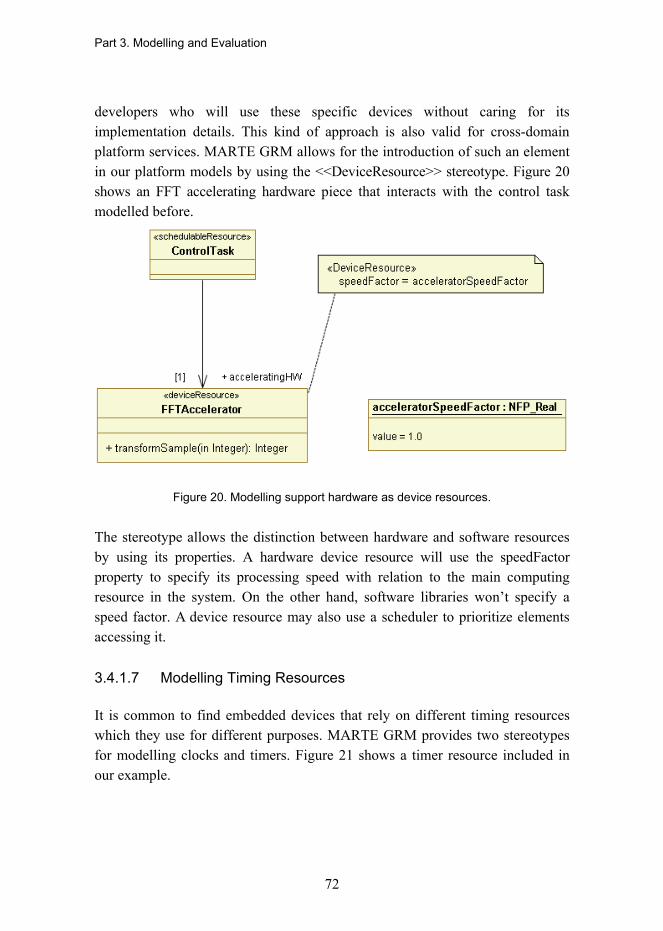
Part 3. Modelling and Evaluation
72
developers who will use these specific devices without caring for its implementation details. This kind of approach is also valid for cross-domain platform services. MARTE GRM allows for the introduction of such an element in our platform models by using the <<DeviceResource>> stereotype. Figure 20 shows an FFT accelerating hardware piece that interacts with the control task modelled before.
Figure 20. Modelling support hardware as device resources.
The stereotype allows the distinction between hardware and software resources by using its properties. A hardware device resource will use the speedFactor property to specify its processing speed with relation to the main computing resource in the system. On the other hand, software libraries won�t specify a speed factor. A device resource may also use a scheduler to prioritize elements accessing it.
3.4.1.7 Modelling Timing Resources
It is common to find embedded devices that rely on different timing resources which they use for different purposes. MARTE GRM provides two stereotypes for modelling clocks and timers. Figure 21 shows a timer resource included in our example.

Part 3. Modelling and Evaluation
73
Figure 21. Modelling a timer.
As depicted in the diagram, we have now added a timer that will periodically inform the system scheduler that it is time to reschedule its managed resources . Clocks are defined in a very similar way. To obtain further information on modelling timing resources please refer to the MARTE GRM specification.
3.4.1.8 Further Refining Platform Structural Models
In many cases the MARTE GRM sub-profile is expressive enough to describe platform architectures; however, in certain cases it is possible that the platforms models may be too generic for the application under construction or with regard to further phases of the development process (e.g. application designs at chip level, L1). If this is the case, MARTE provides two specific and more concrete subprofiles for software and hardware description: the MARTE Software Resources Modelling (SRM) subprofile and the MARTE Hardware Resources Modelling (HRM) subprofile respectively.
3.4.2 Behaviour View
According to MARTE GRM: �Resources are used to model the execution platform from a structural point of view, while the resource services supply the behavioural point of view.�

Part 3. Modelling and Evaluation
74
According to MARTE SRM: �The multitask-based method aims at designing applications as a set of units executing concurrently and interacting (i.e., communicating and synchronizing) via specific mechanisms provided by a specific execution support. That support is in charge of real-time and embedded features (e.g., time constraints, determinism and memory footprint). It provides a set of resources and services through its application programming interface (API).�
According to MARTE HRM: �Typically, an HW_Resource provides at least one HW_ResourceService, and may require some services from other resources. Each HW_ResourceService could be detailed by many views to describe its behaviour patterns. The resource services (HW_ResourceService) are not explicitly specified as they are mainly deduced from the nature of the resource and they should be fully listed only if such level of detail is needed.�
In addition to the behaviour descriptions of high-level core and optional services of GENESYS, there are various execution support services like transferring data, sharing resources, communications and synchronization of tasks.
The behaviour view is presented as the interfaces and their state machine descriptions (i.e. protocol) of the above mentioned services.
Regarding the methodology framework, in order to model the behaviour of the platforms, UML behaviours (i.e. activity, sequence and state machine diagrams) could be useful to model interactions within the platforms.
In order to reflect how platform behaviour can be modelled, an operating system round-robin scheduling pattern is modelled. The example, which is based on [Douglas 2002], describes a round-robin scheduling algorithm by a class diagram (structural view) and a sequence diagram (behaviour view). The model elements that complete the pattern have been stereotyped according to the GRM.
The round-robin pattern schedules a set of ordered processes with static priorities by assigning time-slots to each of them. Once each process completes the processing time it is pre-empted and the processor is assigned to the next process in the list.

Part 3. Modelling and Evaluation
75
Figure 22. Structural view for a scheduling pattern.
The class diagram in Figure 22 describes the main elements involved in the round-robin concurrent pattern. As shown, a system scheduler is interrupted by a timer that is has been previously configured at initialization time. The scheduler assigns time-slots to execution threads which are characterized by their control blocks and stacks. Task control blocks describe the initial addresses of each task and stacks refer to the memory segments assigned to each task for storing temporal variables, a parameter or return values for system calls.
In order to describe the behaviour of the platform, a possible scenario is provided in Figure 23.
In order to facilitate a link between the models and the analysis/simulation tools, the methodology framework provides the option of using opaque behaviour UML model elements. Opaque behaviours are defined by pieces of code or pseudo-code regarding it specification; therefore, using these approach, it is a simple task to establish a link between the UML2+MARTE models and other modelling languages like SystemC or BIP.
Each element in an architectural view represents real hardware and software parts. Each element has, therefore, a behaviour that is implicit to that component�s nature. Behavioural views capture these behaviours and enable simulation and testing tools to draw early conclusions from system design models.
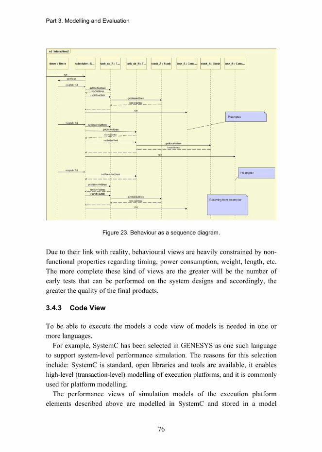
Part 3. Modelling and Evaluation
76
Figure 23. Behaviour as a sequence diagram.
Due to their link with reality, behavioural views are heavily constrained by non-functional properties regarding timing, power consumption, weight, length, etc. The more complete these kind of views are the greater will be the number of early tests that can be performed on the system designs and accordingly, the greater the quality of the final products.
3.4.3 Code View
To be able to execute the models a code view of models is needed in one or more languages.
For example, SystemC has been selected in GENESYS as one such language to support system-level performance simulation. The reasons for this selection include: SystemC is standard, open libraries and tools are available, it enables high-level (transaction-level) modelling of execution platforms, and it is commonly used for platform modelling.
The performance views of simulation models of the execution platform elements described above are modelled in SystemC and stored in a model

Part 3. Modelling and Evaluation
77
library. Based on the selected platform configuration, the platform simulation model is instantiated from these library elements. It should be noted that for a full system performance simulation, an abstracted application model needs to be transformed (e.g. through code generation) or described in SystemC.
Representations in other languages may be needed in the system realization phase, but they are not addressed here.
3.5 Platform Module Library
A Platform Module Library provides the ready-made services defined by the reference architecture template. All definitions of platform services have three dimensions: abstraction, integration and aggregation (Figure 24). These dimensions have different purposes. Each service has two abstraction levels: model and code/implementation, which are intended for the use of different stakeholders, e.g. managers vs. testing people. Both abstraction levels have been introduced in the previous sections. The integration level defines the scope of a service; the platform service can be applicable on one, two or all integration levels (chip (L1), device (L2), open/closed system (L3)). The definition of the integration level is a property of a service that guides the architect to select a proper service for the platform architecture under work. The aggregation dimension is used for separating common services from variable services and managing their relationships. Thus, the dependencies between services are defined by the aggregation dimension that is implemented as a taxonomy of services.
Figure 24. Dimensions of platform services specifications.

Part 3. Modelling and Evaluation
78
The service taxonomy categorizes services into useful groups of services, which make it easy for the platform architect to find a service that fits to a platform architecture design. Figure 25 depicts one possibility for clustering services; core services are used in each GENESYS compatible system, i.e. it is to be checked that all core services have been used in the platform architecture design. Other services are optional and embody variability that has to be managed by the module library management mechanisms. Optional services, e.g., Networking, Security and Resources service class in Figure 25, need definitions of their relationships with core and other optional services, service specific properties and rules that help in selecting, configuring and using a service in architecture design and evaluation phases. These definitions specify explicitly how to deal with variability, i.e. they define facts and rules for variability management. The implementation of variability mechanisms depends on the organization who instantiates the platform module library. Thus, there can be different kinds of taxonomies, depending on the usage of the platform module library.
Platform ModuleLibrary
Core Service
Common Time
Monitoring
Communication
Periodic
Sporadic
Steaming
Configuration
Management Service
Resource
Data
QoS
Messaging
Eventing
Communication
Comput ing
Boot
Security
RN-generator
Dist ributed application
Non-volat ile memory
Job
State
System
Component
Platform
FaultToleranceError Correction
Redundancy mgmt
Program Flow mgmt
Protected Channels
ReplacementDistributed Application
Job
Service
Derived Time
Logging
Synchronization
Execut ion
Application
Encryption
Identification
Optional services goup n
Platform
IP-Core
Routing
***
Figure 25. An initial taxonomy of platform services.

Part 3. Modelling and Evaluation
79
3.6 Integration and Development of Platform Services
In this section we will try to describe how platform services are used as part of the platform models in the methodology framework. Platform services are a group of core and optional services that define the reference architecture template. Each cross-domain architecture style compliant development at each integration level (L1, L2, L3c and L3o) must implement all the core services defined at that level plus a set of optional services specific for the current design. Therefore, applications will rely on the services provided by the underlying platforms. This kind of interaction requires the definition of an interface between which applications interact with the services. Furthermore, each platform service will be defined by its behaviour.
Moreover, the reference architecture template has been defined as an open architecture, able to evolve and adapt to new requirements by adding and changing existing platform services. Therefore, the methodology framework must support the design, development and analysis of new platform services.
3.6.1 Interfacing with Platform Services
System designers using the reference architecture template need are provided with a series of services that simplify the design and implementation tasks. These services are instantiated as part of the platform architecture that supports the applications. Following the approach described in Section 3.4, platform services can be seen as black boxes that provide the designer with higher level functionalities. Figure 26 shows an example core service, the Periodic Exchange of Messages Service.
Figure 26. Periodic Exchange of Messages Service API.

Part 3. Modelling and Evaluation
80
The service description is therefore modelled as a software library API, describing the available interfaces of the GENESYS service as well as the inputs and outputs. This representation might be sufficient for platform designs; however, in order to perform non-functional analyses on the system models a more detailed approach is needed. It is important to note that the API operations are stereotyped with MARTE::GRM <<GRService>>, which denotes the definition of the service interfaces for the clients.
This kind of representation is appropriate for the structural view of the platform architecture models.
3.6.2 Describing the Behaviour of the Services
Each of the GENESYS platform services is treated from the designer�s point of view as a black box that provides him/her with some functionality. In order to fully describe them we still need to add a behavioural description.
As we discussed already in previous sections of this deliverable, the UML+MARTE modelling language provides several mechanisms to represent the behaviour: state machine diagrams, activity diagrams, collaboration diagrams and sequence diagrams. Each of them is preferable for different applications; however, as we defined previously, the behavioural representation which is the most widely used among analysis tools is the state machine. MARTE provides some stereotypes (already described in previous sections) that allow the addition of non-functional information to the behavioural diagrams.
3.6.3 Design Process for New Platform Services
The reference architecture template is an open and evolvable platform which can adapt itself to the new challenges of the embedded systems market. Therefore, the methodology framework must support the design and development of new platform services.
From the point of view of a designer, a new platform service does not differ in concept from the development of a concrete application within the scope of the cross-domain architecture. The design of a new service must go through the six phases of the development process. However, the application models must clearly state the interface (API) of the service under design using the <<GRService>> stereotype. Figure 27 shows an example of this.

Part 3. Modelling and Evaluation
81
Figure 27. The <<GRService>> stereotype in new services design models.
3.7 System Allocation / Configuration / Refinement
The System Allocation / Configuration / Refinement phase of the GENESYS process model is related to the mapping of the applications to the platform architecture elements that will support their execution.
This phase includes an allocation view, the platform architecture configuration view and additional information, e.g. probabilities of state transactions, needed for quality evaluation purposes.
The allocation view defines how applications and services are deployed on the computing and communication resources provided by the execution platform. Typically, platform architecture needs to be configured according to parameters. Additional information required for specific evaluation methods is provided by adding the required information to the models provided by the earlier design phases. An allocated system contains all the necessary information to implement the final product. If the vertical model transformation is supported, simulation and target code can be generated from the validated system architecture models.
The MARTE profile includes a specific sub-profile Alloc that allows a designer to specify which application elements will be associated to which platform resources. In this section we will use again the cruise control system (CCS) example to illustrate allocation modelling in MARTE. Figure 28 depicts the platform model that will support the execution of the controller of the system.

Part 3. Modelling and Evaluation
82
Figure 28. Platform model of the CCS controller.
The platform model of the cruise control system consists of a CPU managed by a system fixed priority scheduler. Three threads have been defined, all of them hosted by the system scheduler. Lastly, two shared protected variables have been defined, each of them with a blocking call for acquiring and releasing the variable lock (i.e. a mutex).
The allocation is performed using the structural views of both application and platform models and using the <<Allocate>> stereotype on UML abstraction dependencies. The <<Allocate>> stereotype allows for further describing the nature and kind of the allocation as well as any constraints to be applied during the allocation process. Additionally, both application and platform elements are stereotyped with <<Allocated>>. The reader can find more information of the stereotypes and their properties from the MARTE profile, Section 11.
Figure 29 shows the structural view of the application model allocated on top of the structural view of the platform model. Each of the operations and receptions in the controller has been allocated on the three threads and the passive protected units have been mapped to mutex-protected variables.
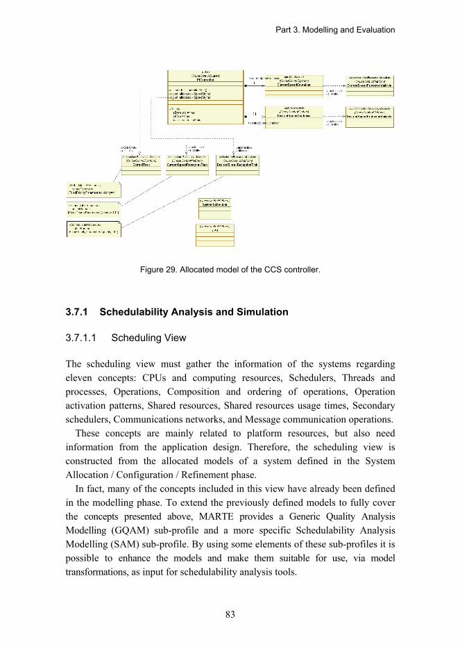
Part 3. Modelling and Evaluation
83
Figure 29. Allocated model of the CCS controller.
3.7.1 Schedulability Analysis and Simulation
3.7.1.1 Scheduling View
The scheduling view must gather the information of the systems regarding eleven concepts: CPUs and computing resources, Schedulers, Threads and processes, Operations, Composition and ordering of operations, Operation activation patterns, Shared resources, Shared resources usage times, Secondary schedulers, Communications networks, and Message communication operations.
These concepts are mainly related to platform resources, but also need information from the application design. Therefore, the scheduling view is constructed from the allocated models of a system defined in the System Allocation / Configuration / Refinement phase.
In fact, many of the concepts included in this view have already been defined in the modelling phase. To extend the previously defined models to fully cover the concepts presented above, MARTE provides a Generic Quality Analysis Modelling (GQAM) sub-profile and a more specific Schedulability Analysis Modelling (SAM) sub-profile. By using some elements of these sub-profiles it is possible to enhance the models and make them suitable for use, via model transformations, as input for schedulability analysis tools.

Part 3. Modelling and Evaluation
84
First, the stereotype provided by MARTE is <<SaExecHost>>, which enriches the information already provided by the <<ComputingResource>> and <<Scheduler>> stereotypes adding some extra properties (in fact, this stereotype inherits the properties from <<ComputingResource>> and <<Scheduler>>).
To use the latter stereotype we create a new class that is related with a scheduler and a computing resource, and which inherits all the values of the properties from <<ComputingResource>> and <<Scheduler>> from them. Figure 30 shows an example of defining a <<SaExecHost>> and relating it to the platform elements.
Figure 30. Example of a <<SaExecHost>> definition.
Second, following with the structural definition of the schedulability analysis contexts, it is important to take the shared resources into account. The stereotypes used for platform definitions, <<MutualExclusionResource>> and <<SynchronizationResource>>, define the platform resources. However, these stereotypes do not model the interactions between operations (i.e. threads) and shared resources. To include this information, the MARTE provides the <<SaSharedResource>> stereotype to represent shared resources along with the <<GaAcqStep>> and <<GaRelStep>> stereotypes to model the interactions between operations and resources.
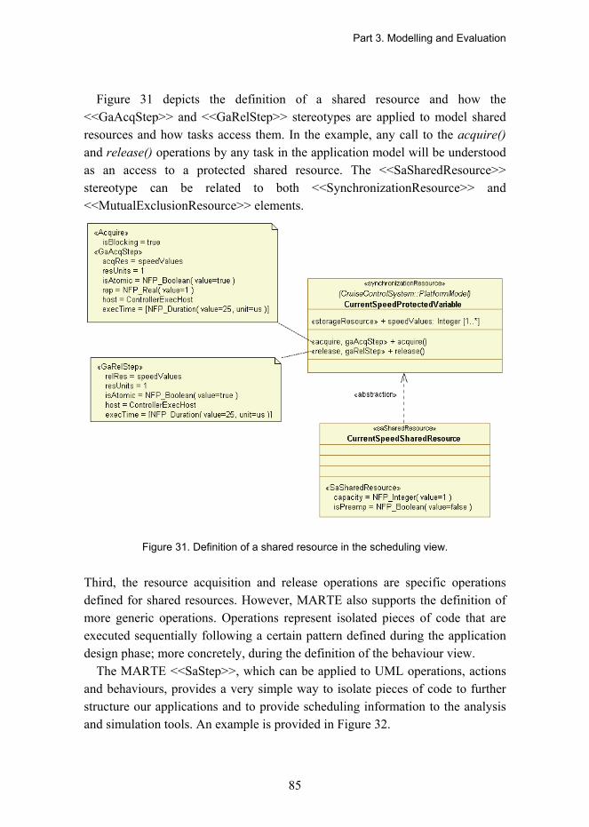
Part 3. Modelling and Evaluation
85
Figure 31 depicts the definition of a shared resource and how the <<GaAcqStep>> and <<GaRelStep>> stereotypes are applied to model shared resources and how tasks access them. In the example, any call to the acquire() and release() operations by any task in the application model will be understood as an access to a protected shared resource. The <<SaSharedResource>> stereotype can be related to both <<SynchronizationResource>> and <<MutualExclusionResource>> elements.
Figure 31. Definition of a shared resource in the scheduling view.
Third, the resource acquisition and release operations are specific operations defined for shared resources. However, MARTE also supports the definition of more generic operations. Operations represent isolated pieces of code that are executed sequentially following a certain pattern defined during the application design phase; more concretely, during the definition of the behaviour view.
The MARTE <<SaStep>>, which can be applied to UML operations, actions and behaviours, provides a very simple way to isolate pieces of code to further structure our applications and to provide scheduling information to the analysis and simulation tools. An example is provided in Figure 32.

Part 3. Modelling and Evaluation
86
Figure 32. An example of the <<SaStep>> stereotype for isolating pieces of code.
Fourth, there exist some operations that imply the sending/receiving of messages using some kind of communication media. These operations have to be treated differently from normal operations. MARTE defines two stereotypes for model communications from a schedulability point of view:
• <<SaCommHost>>, which represents communication networks as well as any scheduling policy that could be defined in those networks, and
• <<SaCommStep>>, which models operations that imply a communication through any communications media.
Figure 33 shows how to introduce these stereotypes in the scheduling view of the systems. As it can be seen from the figure, the <<SaCommStep>> stereotype is appropriate to be applied to UML signal receptions to include scheduling information.
Figure 33. Modelling communications for schedulability analysis in MARTE.
Finally, it is important to address the fact that all other concepts that have not been explicitly treated here are already covered by the stereotypes used in the

Part 3. Modelling and Evaluation
87
earlier defined views of the system models. For example, the activation patterns of the tasks can be modelled using the <<RtFeature>> stereotype from the MARTE HLAM sub-profile. The reason for doing this is because the activation patterns of the tasks is an application design issue, even if information is used for schedulability analyses and simulations. The same is true for secondary schedulers, which have already been covered in the platform design phase. The stereotype <<SecondaryScheduler>> in the GRM subprofile captures this concept in the system models.
3.7.1.2 Analysis and Simulation Tools
As has been outlined in the previous sections, models can be used to capture the most significant structural, behavioural and non-functional information of the systems. This information enables not only source code generation through transformations, but also early testing and analysis. However, different analysis tools often employ different input data formats and it is difficult to make them interoperate. A more abstract language, along with model transformations provides a tool-independent framework for system analysis and testing. This section describes the views that must be added to the existing application models and how the obtained models can be transformed into input models for three different schedulability analysis tools: Cheddar [Singhoff 2004], MAST [MAST 2008] and TIMES [Amnell 2003].
Early detection and correction of system vulnerabilities and errors is increasingly important for embedded software developers; especially for those developers working with safety critical software. Early detection of software defects may reduce the costs derived from the correction of the error. Among the many vulnerabilities that can be detected in an early development stage, schedulability is one of the most recursive topics in the researchers� community.
Several methods and tests have been developed to analyze the schedulability in real-time systems [Liu 1973, Tindell 1994a, Sha 1990, Tindell 1994b]. These tests often require different information from the analyzed system as input. Models provide a good means for capturing this information in a structured way. In order to obtain the necessary concepts that should be included in the scheduling view to enable this kind of testing and analysis, three open-source schedulability analysis and simulation tools have been used: Cheddar, MAST and TIMES. Each of the latter tool suites employs a different set of concepts to create the input models for their simulation and analysis tools. In the following

Part 3. Modelling and Evaluation
88
lines we provide a short overview of the tool suites as well as a brief description concepts involved in their metamodels.
Cheddar
Cheddar is an open source schedulability analysis and simulation toolkit (Figure 34). It was first conceived to be an AADL models analyzer. It has been developed on top of OCARINA [Ocarina 2008], a toolsuite for manipulating AADL models.
Cheddar provides a graphical user interface that allows users to model the application they want to analyze and a simulator which computes simulated schedules and feasibility tests. Although Cheddar supports a great number of scheduling policies and schedulability tests, there are cases where existing schedulers do not match the particularities of a given system. For those cases, Cheddar offers the possibility of defining new schedulers and it is able to analyze the systems according to new scheduling policies.
The schedulers supported by Cheddar for simulation and feasibility analysis are: Rate Monotonic (RM), Deadline Monotonic (DM), Earliest Deadline First (EDF), Least Laxity First (LLF), POSIX 1003b fixed priority scheduler and Maximum Urgency First (MUF). The tool also supports the inclusion of shared resources into the system models.
Figure 34. Extract of the Cheddar metamodel.
Part 3. Modelling and Evaluation
89
In order to perform schedulability analyses, Cheddar uses system XML models as input. We will briefly overview the concepts included in the Cheddar metamodel depicted in Figure 34.
• Processor. Computing resources are modelled in Cheddar as processors. Each processor has associated a certain scheduler type and a name. Schedulers can be defined as preemptive or non-preemptive and a quantum value can be specified.
• Address Space. Address spaces model memory areas reserved for a certain process in a processor. Tasks are allocated in an address space associated with a processor. An address space element has a name and must have a hosting processor. Additionally, an address space may be given a secondary scheduler that will override the primary processor for the tasks allocated to it. Lastly, memory properties can be specified in order to perform utilization tests.
• Task. A task element represents an execution thread running within a certain process. Again, a task element has a name and a hosting address space. A task may have many different parameters that affect them in different scheduling contexts.
• Resource. The element resource of the Cheddar metamodel represents resources shared by different tasks in a system (i.e. critical sections). A shared resource is defined by its name, and its hosting processor and process, and it has a number of extra properties used to specify the number of tasks that may access it simultaneously, the concrete tasks that require the resource and the access protocol.
• Task Precedence. Cheddar models allow the insertion of some behavioural aspects in the models. A task precedence element indicates that a task must be completed before another one may start its execution.
• Message Dependency. Cheddar models use message dependencies to include message-based interactions between senders and receivers. A message element must be defined and related to a message dependency. A message element is defined by its occurrence properties, its size and its communication timing properties.
• Buffer Dependency. Cheddar models use buffer dependencies to include buffer-based interactions between data providers and consumers in streaming

Part 3. Modelling and Evaluation
90
interactions. In similar fashion to message dependencies, a buffer element must be defined and related to a buffer dependency. It is important to note that buffers may only be defined in Cheddar as inter-task communication systems on a local host. A buffer element is defined by the hosting elements (i.e. processor and address space), its size, its queuing policy and the buffer users (i.e. a set of tasks). Buffers can be analyzed in Cheddar using buffer usage simulations and feasibility tests.
MAST
MAST is a toolsuite for modelling and analyzing real-time applications. It has its own metamodels to create the models needed by the analysis and simulation tools. MAST tools make use of the concepts introduced in the metamodels to analyze and simulate real-time applications and provide the results.
MAST supports a variety of scheduling analysis methods: RM, EDF and Holistic. The tool suite also includes a scheduling simulator engine. MAST includes a metamodel for modelling real-time applications and systems. The following paragraphs will briefly cover the concepts included in the MAST metamodel and the properties associated with them (see Figure 35 for further details). Further information about the MAST metamodel can be found in [Medina 2005].

Part 3. Modelling and Evaluation
91
Figure 35. Extract of the MAST metamodel.
• Regular Processor. Regular processor elements represent computing units in real-time application models. A processor in MAST is defined by its name, its timing constraints, its interrupt priority range and its speed factor. A processor may also include a timer.
• Primary and Secondary Schedulers. A primary scheduler represents the main scheduling resource in an operating system. It is defined by an identifier, a host processing unit (i.e. a processor or a network) and a scheduler type (i.e. Fixed Priority or EDF). Secondary schedulers represent tasks that contain a certain scheduling resource that manages a list of tasks.
• Regular Scheduling Server. A regular scheduling server represents the structure of a thread in an operating system, that is, the resources that support the creation of threads, and it owns a series of executable code. A scheduling server is defined by its identifier, the scheduler in charge for managing it and the scheduling policy parameters that will be applied to it

Part 3. Modelling and Evaluation
92
and to the shared resources accessed by it. Note that these parameters must be compatible with the host scheduler.
• Simple Operation. A simple operation represents a small amount of executable code which is executed in a regular scheduling server. Simple operations are defined by an identifier and the timing characteristics that affect its execution. A simple operation may also override the priority defined for the scheduling server and it may also use/lock/unlock a list of shared resources.
• Composite and Enclosing Operations. The MAST metamodel allow the introduction of small behavioural aspects in the models in a similar way to Cheddar. In order to establish an order of precedence between different simple operations composite operations are used. This kind of operation is defined by a list of simple operations that are executed consecutively. On the other hand enclosing operations model higher level operations that contain unique code as well as calling other simple operations. Enclosing operations must specify their timing parameters independently from the simple operations enclosed within them.
• SRP, Priority Inheritance and Immediate Ceiling Resources. These three elements represent shared resources in MAST. An SRP resource represents a non-managed resource or a resource managed by a user-defined protocol, while the other two represent shared resources whose access is managed by priority modification protocols.
• Packet-Based Network. Both the MAST metamodel and its analysis techniques provide support for distributed real-time systems. A packet- based network represents the most basic communication media for transmitting messages between tasks located in remote processing resources. A network is defined by a series of parameters: identifier, speed factor, throughput, transmission type, maximum blocking time and maximum/minimum packet sizes. Moreover a network must have a list of network drivers that manage the messages.
• Message Transmission. A message transmission element represents a special kind of operation that implies the action of sending a message through a network. This kind of operation requires the specification of the message size related to it.
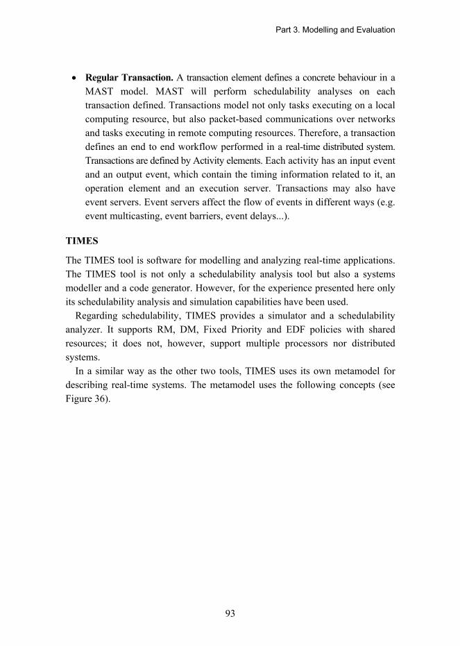
Part 3. Modelling and Evaluation
93
• Regular Transaction. A transaction element defines a concrete behaviour in a MAST model. MAST will perform schedulability analyses on each transaction defined. Transactions model not only tasks executing on a local computing resource, but also packet-based communications over networks and tasks executing in remote computing resources. Therefore, a transaction defines an end to end workflow performed in a real-time distributed system. Transactions are defined by Activity elements. Each activity has an input event and an output event, which contain the timing information related to it, an operation element and an execution server. Transactions may also have event servers. Event servers affect the flow of events in different ways (e.g. event multicasting, event barriers, event delays...).
TIMES
The TIMES tool is software for modelling and analyzing real-time applications. The TIMES tool is not only a schedulability analysis tool but also a systems modeller and a code generator. However, for the experience presented here only its schedulability analysis and simulation capabilities have been used.
Regarding schedulability, TIMES provides a simulator and a schedulability analyzer. It supports RM, DM, Fixed Priority and EDF policies with shared resources; it does not, however, support multiple processors nor distributed systems.
In a similar way as the other two tools, TIMES uses its own metamodel for describing real-time systems. The metamodel uses the following concepts (see Figure 36).

Part 3. Modelling and Evaluation
94
Figure 36. Extract of the TIMES metamodel.
• Task table. Every TIMES model owns a single task table element. The task table defines the scheduling policy that will be applied to the tasks allocated in it.
• Task. A task represents a process/thread in the system. Since TIMES can only handle single processor systems, all the tasks are allocated in a single task table with a single scheduling policy. A task is defined by its worst case execution time, period, deadline, offset, priority and activation pattern (controlled, periodic or sporadic). A task may also use shared resources. In the latter case, each task must address the instants in which it accesses each shared resource.
• Semaphores. TIMES allows the definition of mutexes between tasks. They are modelled using only a name, since TIMES does not support priority inheritance access protocols.
• Task precedence. The TIMES metamodel includes the possibility of defining a certain order of precedence between tasks in the system.

Part 3. Modelling and Evaluation
95
3.7.1.3 Concepts of Scheduling View
Regarding the concepts covered by each of the analyzed tools it is easy to see that many of the concepts are covered in various metamodels differently. Therefore, the introduction of these concepts in the models using a more abstract modelling language provides designers with a higher level tool independent framework.
Table 11 maps the elements present in the three metamodels with the concept they model.
In order for the models to be abstract enough to be used with any of these three analysis and simulation tools, the scheduling view, which can be partly included in other model views, must contain at least the eleven concepts described in the table above.
It is important to note that the concepts defined in the scheduling view refer to both platform and application elements and, thus, the scheduling view should be defined/created on top of the allocated model in the system refinement / allocation phase.

Part 3. Modelling and Evaluation
96
Table 11. Comparison of the concepts of three schedulability analysis tools.
Concept Representation in...
Cheddar MAST TIMES
1. Single and multi-core processors
Processor
Single and multi-core(s)
Regular Processor
Single and multi-core(s)
-
2. Scheduler Processor scheduler Primary Scheduler Task Table
3. Threads/processes Task Regular Scheduling Server Task
4. Execution code
Parameters: worst case execution time, period, deadline, etc.
Task (each task represents a single operation)
Simple/Composed/ Enclosed operations
Task (each task represents a single operation)
5. Complex operations
Execution ordering Task Precedence
Composed/Enclosed Operations + Transactions
Task precedence
6. Shared resources
To be treated in schedulability analysis
Represent mutexes, semaphores, monitors etc.
Resource
SRP, Priority Inheritance and Immediate Ceiling Resources
Shared Resources
7. Triggers Task types Transaction Events Task (behaviour field)
8. Relationships between executing threads and shared resources
Resource �(tasks accessing a concrete resource)
Resources to lock/unlock lists
Task (semaphores field)
9. Secondary schedulers built on top of native scheduler of an operating system
Address Space Secondary Scheduler -
10. Communications network - Packet-Based
Network -
11. Operations that send messages through a network
Message Dependency
Message Transmission -

Part 3. Modelling and Evaluation
97
3.8 Quality Evaluation
The Quality Evaluation methods introduced in this section (phase 5 in Figure 3) give support for evaluating the following quality properties:
• Performance • Power/energy efficiency • Dependability including reliability, availability and safety • Composability, and • Evolvability.
Quality attributes can be classified into two categories; functional qualities, which are observable at execution time (i.e. execution qualities), and non-functional qualities, which are observable during the product life cycle (i.e. evolution qualities). Functional qualities, e.g. performance and dependability, express themselves in the behaviour of the system, while non-functional qualities, e.g. composability and evolvability, are embodied in the static structures of systems.
The interest of the quality attributes for system architecture is in the manner that quality attributes interact with, and constrain, each other, and how they affect the achievement of other quality attributes. Therefore, a set of quality attributes are to be handled at the same time and tradeoffs between quality attributes are to be calculated and managed. For example, dependability is a concept that includes four quality attributes: reliability, availability, safety and security. Moreover, a new concept �trustworthiness� focuses on a holistic view of quality including the following attributes: correctness, safety, availability, reliability, performance, security and privacy. The holistic approach aims at applying multidimensional optimization techniques onto a set of quality attributes that can have intrinsic and/or extrinsic relationships on other quality attributes. An intrinsic relationship exists if one quality attribute affects another. For example, models to predict reliability depend on a system�s anticipated performance. This relation between reliability and performance is intrinsic. Extrinsic relationships occur when attributes behave in an opposing way, e.g. an increase in reliability decreases performance. In this case, the relation between reliability and performance is extrinsic. However, the relations between two attributes do not exit per se but rather they are properties of system architecture [Hasselbring 2006].
Part 3. Modelling and Evaluation
98
Although the focus of this chapter is in the Quality evaluation phase, in order to evaluate quality, several assumptions are made about the information inserted into models during the preceding phases, i.e. requirements specification and architecture design. Therefore, each evaluation method also defines how the use of the method should be supported in the preceding modelling phases.
In the following sections, the quality evaluation methods specific for each quality attributes (QA) are introduced. First, the execution quality evaluation methods are defined and thereafter the evolution quality evaluation methods in the prioritized order mentioned above.
3.8.1 Performance Evaluation
Performance evaluation means a process of estimating, through using performance models in quantitative terms, what the performance properties of the system being designed when implemented would be, whereas after implementation it is more a question of measuring the values of properties (the latter is not addressed in the sequel).
Performance evaluation in the context of real-time embedded systems development tries to provide insight into three main issues:
• Responsiveness: Is the system capable of producing responses to user (external) service requests in defined response times or according to a defined throughput?
• Resource adequacy/utilization: Does the system have resources and is their capacity enough for the currently planned applications? How efficiently are the resources utilized?
• Scalability: Does the system facilitate extensions/reductions and scale up/down resources and is their capacity enough to accommodate future applications / changes in applications?
Performance evaluation methods can be classified according to three main classes: analytical methods, simulation methods and monitoring methods [Jain 1991].
Analytical performance modelling is typical in the early phases of design and its methods are based on mathematical models of the workload and the system architecture. Markov chains, queuing models and Petri-nets are typical examples of analytical modelling techniques. Analyses are normally based on solving the equations, but simulation is also used as a supporting tool.

Part 3. Modelling and Evaluation
99
In the performance simulation, the execution of a workload with a model of an execution platform is simulated. The workload modelling can be based on several alternatives, e.g. executable programs (real application or benchmark programs), execution traces of programs and stochastic models. Execution platform modelling can be based on e.g. abstract resource capacity models or virtual platform models where instruction-set simulators are used to simulate programmable.
Monitoring/measurement-based approaches need working prototypes of hardware. The prototype is calibrated to gather performance information during the execution of the software.
Future embedded systems integrate an increasing number of concurrent applications on MPSoCs. Therefore, performance evaluation is gaining importance in the industry, while unfortunately also becoming increasingly complex.
Cycle accurate simulations are less and less usable for complex systems, except when investigating a limited part of the system, because the number of cycles that need to be simulated grows (and cycle-accurate SystemC simulations are very slow) and because they need to have all the exact code available. Unfortunately, the processors used in platforms have become so complex that this kind of simulation, with the exact code and memory layout, often remains the only chance for estimating timing properties. The classical obstacles to evaluations at higher level are the non-predictabilities of cache memories, competing requests for resources, and more generally interferences between different activities. Possibilities can appear in applications where situations are diverse enough to allow hiding cache misses and bus conflicts effects behind an averaging at a very coarse grain.
In many cases, what the developers of complex applications need is an evaluation of performance with a coarse, but guaranteed, error margin. The key issue there is predicated upon the existence and capabilities of appropriate tools, and on whether the assumptions that they put on the behaviour of platforms and applications are valid for the system under test. The GENESYS architecture principles on complexity management, component-based design, composability, etc., will allow raising the abstraction level at which performance modelling and evaluation is performed, and should therefore have a significant impact on this situation.

Part 3. Modelling and Evaluation
100
3.8.1.1 Pre-requisites
A number of pre-requisites are needed for doing the evaluation. The following sub-sections browse through how to consider performance in the modelling phases of the GENESYS methodology.
A basic assumption is that the modelling applies UML2 supplemented with the MARTE profile for dealing with NFP modelling.
3.8.1.2 System Requirements Definition
In the requirements specification phase, performance appears as requirements to and/or constraints on the functionality (e.g. response times, throughput,�), execution platform resources (e.g. capacities, energy,�), and the development process itself.
The performance evaluation needs the following input from the requirements modelling:
• Usage scenarios of the system, i.e. service interaction of the user with the system, e.g. a set of representative use cases.
• Service interaction of the main (internal) actors of the system when providing the above services (system behaviour), e.g. as a set of sequence diagrams.
• Related performance requirements/constraints explicitly defined within the above diagrams following the modelling constructs of UML2 with the SysML (and/or MARTE) profile.
In addition to the above usually functionality related (timing, QoS, etc.) requirements and constraints, other global/generic/holistic ones cannot often be associated to specific usage scenarios of the system and they are given as overall requirements and constraints. These shall be fulfilled in the subsequent development and are often sources of evaluation criteria against which to compare evaluation results.
Some of the common NFP attributes for analysis in the GQAM sub-profile of MARTE could possibly (depending on the formalism/elaborateness of the requirements model) be used already here (Table 12).

Part 3. Modelling and Evaluation
101
Table 12. Examples of NFP attributes for requirements model.
Delay (including initial scheduling delay) (respTime).
Time interval between two successive occurrences (interOccTime).
Throughput (executions per unit time) (throughput).
3.8.1.3 Application Architecture Design
In the application architecture design phase, performance appears e.g. as deadlines of activities (tasks), service processing times, and types and amounts of data to be communicated. In the HLAM sub-profile of MARTE, the <<rtf>> stereotype allows for attaching real-time characteristics, e.g. deadlines and durations, to interactions (interfaces) (Table 13).
Table 13. Attributes of the <<rtf>> stereotype.
Property Type Multiplicity Description
utility MARTE_Library::
UtilityType [0..1]
An abstract type. It must be defined by the user. This type enables MARTE to include a semantic description of this service.
occKind
MARTE_Library::
BasicNFP_Types::
ArrivalPattern
[0..1] This property describes the occurrence pattern for the arrival of this element.
tRef
MARTE_Library::
TimedObservations::
TimedInstantObservation
[0..1] This property describes a reference time that will be used for relative time measures.
relDl NFP_Duration [0..1] Relative deadline.
absDl NFP_DateTime [0..1] Absolute deadline.
boundDl NFP_BoundedDuration [0..1] Bounded deadline.
rdTime NFP_Duration [0..1] Time used by the current element to perform its work.
miss NFP_Percentage [0..1] Maximum admissible deadline miss percentage.
priority NFP_Integer [0..1] The priority of this communication.

Part 3. Modelling and Evaluation
102
The GQAM sub-profile of MARTE defines how extra annotations can be attached to design models for analysis in order to describe how system behaviour uses system resources. Workloads describe how system behaviour exercises system resources over time. The central concepts for workload description are workload events triggering behaviour scenarios that are composed of steps.
A Behaviour Scenario captures any system-level behaviour description or any operation in UML, and attaches resource usage to it. Resources are used in three different ways (Table 14):
• Each primitive Step has a host processor used to execute the operation of the step,
• A Step implicitly uses an operating system process which is a SchedulableResource,
• A Step may be a specialized AcquireStep or ReleaseStep to acquire or release a Resource, particularly a logical Resource representing a software resource.
Table 14. NFP attributes for workload elements.
BehaviourScenario Step
hostDemand: NFP_Duration blockingTime: NFP_Duration [*]
hostDemandOps: NFP_Real [*] repetitions: NFP_Real =1
interOccTime: NFP_Duration [*] probability: NFP_Real = 1
throughput: NFP_Frequency [*] priority: NFP_Integer
respTime: NFP_Duration [*]
utilization : NFP_Real [*]
utilizationOnHost : NFP_Real [*]
3.8.1.4 Platform Architecture Design
In platform architecture design phase, performance appears as latencies / processing times of services, capacities of resources, e.g. processor configuration and its properties, and capacities of infrastructure, e.g. communication bandwidth and policies.

Part 3. Modelling and Evaluation
103
In principle, 3 sub-profiles of MARTE can be applied in the platform architecture design: GRM, SRM and HRM. The GRM profile is aimed at high-level modelling of platforms, while SRM and HRM facilitate detailed modelling.
Considering the scope of the GENESYS project, applying the GRM sub-profile seems most appropriate. The central concept of GRM is resource providing services and their corresponding instances.
From the analysis point of view, the GQAM defines resource platform composed of resources being either processing or concurrency resources (Table 15).
Table 15. NFP attributes for different resource types.
Execution host Communication host Communication channel
commTxOverhead: NFP_Duration capacity: NFP_DataTxRate
packetSize: NFP_DataSize
commRcvOverhead: NFP_Duration throughput: NFP_Frequency utilization: NFP_Real
contextSwitchTime: NFP_Duration packetTime: NFP_Duration
clockOvh: NFP_Duration blockingTime: NFP_Duration
schedPriorityRange: NFP_Interval transmMode: TransmModeKind
memorySize: NFP_DataSize utilization: NFP_Real
utilization: NFP_Real
3.8.1.5 System Allocation / Configuration / Refinement
In the system allocation / refinement phase, performance appears as part of the cost function based on which the application functionality (with capacity requirements) will be partitioned and mapped on the resources of the execution platform (with provision of capacities).
The sub-profile Alloc of MARTE describes how application-related design models can be associated to execution platform models. NFP constraints can be added to these associations.
Depending on the type of analysis, system allocation can be a step in the process or it can be implicitly embedded in the analysis modelling as in the SAM and PAM sub-profiles of MARTE.

Part 3. Modelling and Evaluation
104
3.8.2 Performance Evaluation Methods
Performance evaluation can be used at different stages and for various purposes in order to support the system (product) development process:
• Early feasibility analysis/evaluation
• Analysis of impacts of new application / application feature on (existing) execution platform
• Specification/design of new execution platform when targeted applications are characterised
• Supporting design space exploration
• Validation of performance aspects of implemented system.
Consequently, different methods or combinations thereof may be needed. Numerous approaches have been presented in research and many are used in practice. In the sequel, two different approaches are described as examples (Figure 37): the main focus of the first is software architecture performance analysis/evaluation using LQN performance models; the second is aimed at application-platform performance analysis/evaluation using a transaction level simulation of workload models of an application mapped on capacity models of an execution platform.
Figure 37. Input, output and support for performance evaluation.
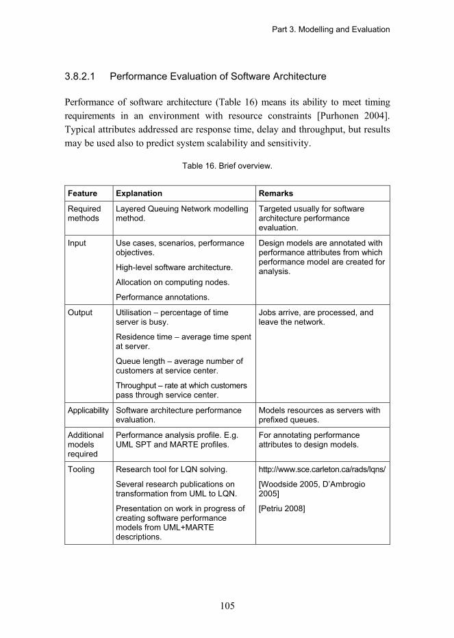
Part 3. Modelling and Evaluation
105
3.8.2.1 Performance Evaluation of Software Architecture
Performance of software architecture (Table 16) means its ability to meet timing requirements in an environment with resource constraints [Purhonen 2004]. Typical attributes addressed are response time, delay and throughput, but results may be used also to predict system scalability and sensitivity.
Table 16. Brief overview.
Feature Explanation Remarks
Required methods
Layered Queuing Network modelling method.
Targeted usually for software architecture performance evaluation.
Input Use cases, scenarios, performance objectives.
High-level software architecture.
Allocation on computing nodes.
Performance annotations.
Design models are annotated with performance attributes from which performance model are created for analysis.
Output Utilisation � percentage of time server is busy.
Residence time � average time spent at server.
Queue length � average number of customers at service center.
Throughput � rate at which customers pass through service center.
Jobs arrive, are processed, and leave the network.
Applicability Software architecture performance evaluation.
Models resources as servers with prefixed queues.
Additional models required
Performance analysis profile. E.g. UML SPT and MARTE profiles.
For annotating performance attributes to design models.
Tooling Research tool for LQN solving.
Several research publications on transformation from UML to LQN.
Presentation on work in progress of creating software performance models from UML+MARTE descriptions.
http://www.sce.carleton.ca/rads/lqns/
[Woodside 2005, D�Ambrogio 2005]
[Petriu 2008]

Part 3. Modelling and Evaluation
106
Evaluation criteria. the evaluation criteria are defined based on the results of the system requirements definition. The scope of the performance evaluation of the software architecture is determined with a performance profile. A profile is a group of use cases that describe the critical usage situations of the system. The use cases are further specified as scenarios. Often one use case has to be described with several concurrent scenarios. The result of this phase in the architecture development is the evaluation criteria i.e. the test specification for the architecture. The evaluation specification describes the scope, the performance objectives, and the evaluation environment. Performance objectives set the individual goals or constraints to each scenario in a profile. Performance objectives can be, for example, goals to the response times or resource utilization.
Software architecture model. Application architecture design results in the description of the software architecture by architectural views (Table 17): a) The Logical view presents the required functionality, b) The Physical view presents the deployment of logical components to the execution nodes, c) The Process view presents the runtime operation of the software in the execution nodes, d) The Development view presents organizational constraints.
Table 17. Architecture views and performance aspects.
View Description Performance
Logical Presentation of required functionality in an implementation-independent way.
� Required functionality
� Complexity estimates
Physical Presentation of deployment of the logical components to the execution nodes.
� Deployment
� Hardware capability
Process Presentation of the runtime operation of the software in the execution nodes.
� Runtime components
� Scheduling and other resource allocation policies
Development Presentation of the modules to be developed in a language-independent way.
� Constraints by development environment
� Development components

Part 3. Modelling and Evaluation
107
Although performance analysis is essentially made from the process view, information from the other views is also needed. The logical view is used for understanding the required functionality. A complexity estimate should be attached to each logical component for which there is still not a good reference solution available. The physical view shows the deployment of the logical components to the hardware platform. It should also provide the estimates or the actual values of hardware capability, for example, the processor capacity and memory size. The process view shows the partition of software to runtime components. In addition, it describes the resource allocation policies. The development view can affect the performance evaluation through constraints set by the organization or used software technology. For example, the organization may require the use of certain design tools to which the evaluation approach should be attached.
Evaluation. Contemporary performance analysis techniques are applied. For example, RMA or queuing based approaches are applied in this phase.
A typical evaluation sequence is depicted in Figure 38.
Figure 38. Performance evaluation of software architecture.
Queuing networks, stochastic Petri nets and stochastic process algebras are usual performance model formalisms.
Queuing networks model each time-consuming resource of a system as a server with a prefixed queue. Networks can be built by connecting servers. Each job that arrives in the network is processed by a server, e.g. CPU. After that, the job is processed by the next server or leaves the network. In an open queuing network, jobs arrive and leave the system. In closed queuing networks, a fixed number of users circulate in the network. The usual parameter values for
Part 3. Modelling and Evaluation
108
queuing models are service times and arrival rate of jobs for each runtime component in the model, and the resources used. Typically a solution to a queuing model gives the average response time to requests as a result. Other results might be average queue length or throughput of nodes.
Stochastic Petri nets combine functional and non-functional properties of software, focus on synchronization and concurrency and allow modelling of resource contention, mutual exclusion and priorities of tasks.
Stochastic process algebras represent a system as a collection of processes, which communicate, interact and synchronize with each other. Performance attributes can be added by stochastic expressions.
Analysis The results are compared to the goal of the evaluation and requirements. The trade-off points are studied. Refinements are proposed based on this analysis. The evaluation report is needed to maintain a design rationale.
Use in GENESYS. Assuming model-based design using UML2 and MARTE in GENESYS provides a good opportunity for adopting a software performance evaluation approach as described above. Three main points are:
Performance properties and attributes need to be annotated to design models. Here the MARTE profile gives a good starting point.
Annotated design models need to be transformed into appropriate performance models (e.g. LQN, SPN or SPA). Much related research exists, but commercial tool support is rare/missing.
Performance models need to be solved/simulated/executed to produce performance data. Again, a lot of related research exists, but commercial tool support is rare/missing.
3.8.2.2 Application-platform Performance Evaluation
The performance modelling and evaluation approach summarized in Table 18 follows the Y-chart model as depicted in Figure 39 [Kreku 2008].

Part 3. Modelling and Evaluation
109
Table 18. Brief overview.
Feature Explanation Remarks
Required methods
Workload modelling method (UML or SystemC).
Platform modelling method at transaction level model abstraction (SystemC).
Targeted for application-platform performance evaluation.
Input Use cases, scenarios, performance objectives.
High-level application software architecture.
Performance model of execution platform.
Performance annotations.
Workload models are allocated on platform models.
Output Utilisations � percentage of time platform resources are busy.
Numbers of load primitives, of service calls, requests and responses performed by resources.
Response and processing times of services.
Workload models send load primitives to platform model to be executed in simulation.
Applicability For evaluation of how application uses platform resources.
Models resources as capacity models of platform hardware and software.
Additional models required
Allocation model. For associating workload models to platform resources.
Tooling Research approach using Telelogic Tau G2 UML tool and OSCI SystemC library.
[Kreku 2008]
Applications are modelled in either UML (Unified Modelling Language) or SystemC domain as workloads consisting of load primitives. The layered hierarchical workload models represent the computation and communication loads the applications place on the platform when executed. The workload models reflect accurately the control structures of the applications, but the computing and communication loads are abstractions derived either analytically, from measured traces or using a source code-compilation approach.

Part 3. Modelling and Evaluation
110
Figure 39. Y-chart model of performance modelling and evaluation.
Layered hierarchical platform models represent the computation and communication capacities the platform offers to the applications. Platform models are cycle-approximate transaction-level SystemC models. The execution platform model is configured from a library of performance models.
The workload models are mapped onto the platform models. Mapping between UML application models and the SystemC platform models is based on the automatic generation of simulation models for system-level performance evaluation. The executable simulation model is based on the open source OSCI (Open SystemC Initiative) SystemC library, extended with configurable instrumentation. The resulting system model is simulated at transaction-level to obtain performance data. The simulation results can be selected for analysis and viewed using visualisation tools.
The approach enables performance evaluation early, exhibits light modelling effort, allows fast exploration iteration, and reuses application and platform models. It provides performance results that are accurate enough for system-level exploration. The simulation performance is good; in an example case study, the simulation speed was one tenth of real time.
Workload models for performance simulation. Workload models are used for characterising the control flow and the loads (amounts of workload primitives {read(), write(), execute()}) of the data processing and communication of applications on the execution platform. The workload models have a hierarchical

Part 3. Modelling and Evaluation
111
structure, where each workload model level consists of a control part and one or more lower level (level-1) workloads (Table 19).
Table 19. Workload element hierarchy.
Workload element name Description
MainWorkload Main workload model W divides into application
workloads Ai:
ApplicationControl CA denotes the common control between the
workloads
ApplicationWorkload Each application workload Ai is constructed of one or
more processes Pi:
ProcessControl CP corresponds to the control between the processes
ProcessWorkload Processes are comprised of function workloads
Fi: ,
StatisticalProcessWorkload Statistical process workload describes the total
number of different types of load primitives
FunctionDistribution Control of statistical distribution for the primitives
DeterministicProcessWorkload Deterministic process workload
FunctionControl CF is control and describes the relations of the
functions, e.g. branches and loops
FunctionWorkload Control flow graphs , where nodes
are basic blocks, and arcs are branches.
StatisticalFunctionWorkload Statistical function workload
BasicBlockDistribution Control of statistical distribution for the primitives
DeterministicFunctionWorkload Deterministic function workload
BasicBlockControl Control of load primitives
BasicBlockWorkload Ordered set of load primitives
AbstractInstruction Load primitive for load characterization
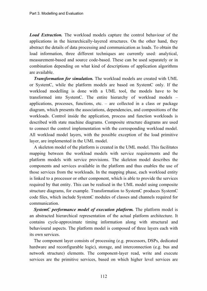
Part 3. Modelling and Evaluation
112
Load Extraction. The workload models capture the control behaviour of the applications in the hierarchically-layered structures. On the other hand, they abstract the details of data processing and communication as loads. To obtain the load information, three different techniques are currently used: analytical, measurement-based and source code-based. These can be used separately or in combination depending on what kind of descriptions of application algorithms are available.
Transformation for simulation. The workload models are created with UML or SystemC, while the platform models are based on SystemC only. If the workload modelling is done with a UML tool, the models have to be transformed into SystemC. The entire hierarchy of workload models � applications, processes, functions, etc. � are collected in a class or package diagram, which presents the associations, dependencies, and compositions of the workloads. Control inside the application, process and function workloads is described with state machine diagrams. Composite structure diagrams are used to connect the control implementation with the corresponding workload model. All workload model layers, with the possible exception of the load primitive layer, are implemented in the UML model.
A skeleton model of the platform is created in the UML model. This facilitates mapping between the workload models with service requirements and the platform models with service provisions. The skeleton model describes the components and services available in the platform and thus enables the use of those services from the workloads. In the mapping phase, each workload entity is linked to a processor or other component, which is able to provide the services required by that entity. This can be realised in the UML model using composite structure diagrams, for example. Transformation to SystemC produces SystemC code files, which include SystemC modules of classes and channels required for communication.
SystemC performance model of execution platform. The platform model is an abstracted hierarchical representation of the actual platform architecture. It contains cycle-approximate timing information along with structural and behavioural aspects. The platform model is composed of three layers each with its own services.
The component layer consists of processing (e.g. processors, DSPs, dedicated hardware and reconfigurable logic), storage, and interconnection (e.g. bus and network structure) elements. The component-layer read, write and execute services are the primitive services, based on which higher level services are
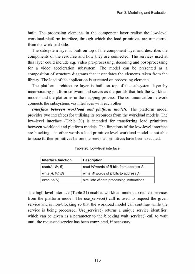
Part 3. Modelling and Evaluation
113
built. The processing elements in the component layer realise the low-level workload-platform interface, through which the load primitives are transferred from the workload side.
The subsystem layer is built on top of the component layer and describes the components of the resource and how they are connected. The services used at this layer could include e.g. video pre-processing, decoding and post-processing for a video acceleration subsystem. The model can be presented as a composition of structure diagrams that instantiates the elements taken from the library. The load of the application is executed on processing elements.
The platform architecture layer is built on top of the subsystem layer by incorporating platform software and serves as the portals that link the workload models and the platforms in the mapping process. The communication network connects the subsystems via interfaces with each other.
Interface between workload and platform models. The platform model provides two interfaces for utilising its resources from the workload models. The low-level interface (Table 20) is intended for transferring load primitives between workload and platform models. The functions of the low-level interface are blocking � in other words a load primitive level workload model is not able to issue further primitives before the previous primitives have been executed.
Table 20. Low-level interface.
Interface function Description
read(A, W, B) read W words of B bits from address A.
write(A, W, B) write W words of B bits to address A.
execute(N) simulate N data processing instructions.
The high-level interface (Table 21) enables workload models to request services from the platform model. The use_service() call is used to request the given service and is non-blocking so that the workload model can continue while the service is being processed. Use_service() returns a unique service identifier, which can be given as a parameter to the blocking wait_service() call to wait until the requested service has been completed, if necessary.

Part 3. Modelling and Evaluation
114
Table 21. High-level interface.
Interface function Return value Description
use_service(name, attr) service identifier id request service name using attr as parameters
wait_service(id) N/A wait until the completion of service id
The platform model includes one or more operating system (OS) models (Figure 40), which control access to the processing unit models of the platform by scheduling the execution of process workload models. The OS model provides both low-level and high-level interfaces to the workloads and relays interface function calls to the processor or other models which realise those interfaces. The OS model will allow only those process workloads which have been scheduled for execution to call the interface functions. Rescheduling of process workloads is performed periodically according to the scheduling policy implemented in the model.
Figure 40. During simulation process workloads are scheduled by the OS model.
SystemC performance simulation. During the simulation of the system model, the workloads send load primitives and service calls to the platform model. The platform model processes the primitives and service calls, advancing the simulation time while doing so. The simulation run will continue until the top-level workload model stops it when the use case has been completed.
Part 3. Modelling and Evaluation
115
The platform model is instrumented with counters, timers and probes, which record the status of the components during the simulation. These performance probes gather information about platform performance, e.g:
• Status probes collect information about utilisation of components and scheduling of processes performed by the operating system models
• Counters count the number of load primitives, service calls, requests and responses performed by the components
• Timers keep track of the task switch times of the OS models and processing times of services.
Once the simulation is complete, the performance probes output the collected performance data to the standard output. The data can be analysed and feedback given to an application or platform design. If the utilisation of components is for example low, lowering the clock frequency can be proposed to platform designers for decreasing power consumption.
Use in GENESYS. Firstly, the approach described above requires abstracted models of applications in the form of workload models that model the control behaviours but abstract data processing and communication as loads. These can be modelled e.g. using UML and MARTE, but also in SystemC. Secondly, transaction-level performance capacity models of the execution platform are needed in SystemC. In case UML and MARTE are used in the workload modelling, the models need to be transformed to SystemC which would require a corresponding generator tool (an add-on to Telelogic Tau G2 UML tool was used in the above example).
Examples of similar approaches. Several approaches having to some extent similar goals but using different formalisms and techniques have been presented in research publications:
SPADE [Lieverse 2000] implements a trace-driven, system-level co-simulation of application and architecture. The application is described by Kahn process networks and symbolic instruction traces generated by the application are interpreted by architecture models to reveal timing behaviour. Abstract, instruction-accurate performance models are used for describing architectures.
The Artemis work [Pimentel 2006] extends SPADE by introducing the concept of virtual processors and bounded buffers. The system-level

Part 3. Modelling and Evaluation
116
simulation environment allows for architectural exploration by applying dataflow graphs to take care of the runtime transformation of coarse-grained application-level events into finer grained architecture-level events that drive the architecture model components.
The basic principle of the TAPES [Wild 2006] is to abstract the involved functionalities by processing latencies and to cover only the interaction of them on the architecture without actually running the corresponding program code. Each sub-function is captured as a sequence of transactions, also referred to as trace, and by storing the trace in the respective architectural resource, which can contain several traces.
MESH [Paul 2005] looks at resources, software, and schedulers/protocols as three abstraction levels that are modelled by software threads on the evaluation host. Hardware is represented by continuously activated, rate-based threads, whereas software threads contain annotations describing the hardware requirements � so-called time budgets that are arbitrated by scheduler threads. Software time budgets are derived beforehand by estimation or profiling.
Koski [Kangas 2006] is an automated SoC design methodology focusing on abstract modelling of application and architecture. This methodology includes early architecture exploration, methods to generate the models from the original design entry and system-level architecture exploration performing automatically allocation and mapping. It also includes a tool chain supporting the defined methodology utilizing a graphical user interface, well-defined tool interfaces, a common intermediate format, and a simulation tool that combines abstract application and architecture models for co-simulation.
Examples of commercial tools:
CoFluent Design (http://www.cofluentdesign.com) provides ESL design tools for modelling and simulating hardware/software systems that allow users to analyze key architectural trade-offs between power consumption, bus/interconnect/processor loads, memory usage and cost. The functional description is a set of communicating processes executing concurrently. The platform model is a set of communicating processes and shared memories linked by shared communication nodes. The transaction level SystemC platform model has performance attributes associated with it.

Part 3. Modelling and Evaluation
117
CoWare Inc. (http://www.coware.com). Platform Architect is a SystemC-based graphical environment for capturing the platform for analysis at transaction-level. It integrates simulation build, simulation run, and system-level analysis controls so that platform developers can rapidly create and validate hierarchical, reconfigurable platforms. The platform designer can create a virtual platform of his design to be distributed to software developers. Software designers then receive a virtual platform package which includes a compiler, a debugger and the platform simulator.
3.8.3 Power/Energy Efficiency Evaluation
Power/energy evaluation and related design and development techniques for uni-processor environments are quite mature research topics. Conventional power estimation approaches use power simulators at gate-level and lead to fairly accurate results. Register-transfer-level (RTL) power simulators aggregate gate-level power data to RTL components to achieve acceptable simulation times.
The situation is different in the case of current and future MPSoCs on which applications of embedded systems and handheld multimedia devices are built, and powered from limited capacity batteries:
The number of gates per chip is approaching a billion, which increases simulation complexity and execution time far beyond the acceptable range.
Systems are designed using IPs coming from different sources in various forms. MPSoCs are often composed of a number of SoCs (that possibly existed before). Therefore gate- or RTL-level (power) information is not usually available.
Systems are becoming software programmable, which emphasises performance-power scaling and power management from the software side. Although the control mechanisms are part of platform (system) software, interactions are necessary with the application software in order to deduce/negotiate/select performance-power/energy policies e.g. by using Quality-of-Service (QoS) categorisation.
Technology scaling also scales nominal power, but more slowly than the number of gates. Furthermore, voltage scaling that was earlier the main means of reducing power is about to stop due to its hitting thresholds. Special low power design and low power silicon processes can help to keep the peak power consumption within some threshold budgets. However, new active means for power/energy management are needed to achieve acceptable average and standby power/energy figures, especially for battery-powered devices. For

Part 3. Modelling and Evaluation
118
example, clock- and/or power-gating of whole computing nodes can be one of such means in a MPSoC. This would require support from system/application software in order to know what can be shut down and what functions and how (to keep QoS) need to be moved to other computing nodes.
It is obvious that to be able to manage power-energy issues, trade-offs, often dynamic, with respect to performance are needed. The applications that are usually considered to transform to embedded software do not consume power-energy per se, but their execution on a MPSoC causes power-energy consumption in the various components of the platform (processors, memories, interfaces, interconnects, power supply / conversion itself etc.). Therefore, there is an interplay of application architecture and platform architecture in handling power/energy issues and an assumption is made that the MPSoC platform contains an appropriate means for planning/deciding (e.g. some kind of power-energy / resource manager) and for controlling (e.g. DVFS controls, clock-gating and/or power-gating).
3.8.3.1 Pre-requisites
A number of pre-requisites are needed for doing the evaluation. The following sub-sections browse through how to consider power/energy in the modelling phases of the GENESYS methodology.
A basic assumption is that the modelling applies UML2 supplemented with the MARTE profile for dealing with NFP modelling.
3.8.3.2 System Requirements Definition
In the requirements specification phase, power/energy appears as requirements to and/or constraints on the functionality and execution platform resources, especially to power supplies, and the development process itself.
The related information in the requirements modelling includes e.g:
• Power source (battery) capacity and its characteristic properties • Operation times with different use profiles • Maximum, average and standby power consumption allowed.
The MARTE profile defines a basic data type NFP_Power and the related unit PowerUnitKind.

Part 3. Modelling and Evaluation
119
3.8.3.3 Application Architecture Design
In the application architecture design phase, various techniques have been proposed to manage/reduce power/energy [Venkatachalam 2005].
One group of work proposes techniques that enable applications to adapt to their runtime environment including e.g:
• Architecture-centric (processes, event handlers, communication mechanisms) transformations of applications using simulators to measure energy consumption
• Trading the accuracy of computations for reduced energy consumption
• Trading the fidelity or quality of data e.g. presented to the user
• Letting applications to �compete� for energy of power resource via �energy futures� distributed by OS resource management.
The idea in another group of techniques is to provide mechanisms (APIs) so that applications can give hints (like start times, deadlines, execution times and I/O resource usage) to e.g., the OS that can further control the power/energy management mechanisms of hardware.
Furthermore, holistic approaches have been researched that integrate information from multiple levels (applications, compilers, middleware, OS�s, hardware) into a power management framework.
As can be seen above, the techniques are domain-, application-and even case-specific. The GRM sub-profile of MARTE gives concepts ResourceAmount and ResourceUsage that can possibly offer useful mechanisms for power/energy modelling in the application architecture design phase. The attributes of ResourceUsage are presented in Table 22.
Table 22. UsageTypedAmount.
execTime: NFP_Duration [ *]
msgSize: NFP_Dat aSize [*]
allocatedMemory: NFP_DataSize [ *]
usedMemory: NFP_DataSize [*]
powerPeak :NFP_Power [*]
enery:NFP_Energy [*]

Part 3. Modelling and Evaluation
120
These power/energy issues are tightly related to performance, and the related modelling issues are useful also here.
3.8.3.4 Platform Architecture Design
In the platform architecture design phase, power/energy appears as energy consumptions of services of resources and infrastructure.
In addition to the GRM sub-profile of MARTE, the SRM and HRM may provide a means to handle power/energy. The ResourceAmount and ResourceUsage concepts of GRM profile are available in the SRM. The HRM contains a package called HW-Power. It defines e.g., concepts HW_Battery, HW_PowerSupply and an HW_PowerDescriptor, the last one being related with resource services. Their attributes are presented in Table 23.
Table 23. NFP attributes for HW_Power.
HW_Battery HW_PowerSupply HW_PowerDescriptor
capacity: NFP_Energy suppliedPower: NFP_Power consumption : NFP_Power
dissipation: NFP_Powerl
3.8.3.5 System Allocation / Configuration / Refinement
In the system allocation / configuration / refinement phase, power/energy appears as part of the cost function based on which the application functionality (with power/energy usage) will be partitioned and mapped on the resources of the execution platform (with provision of power/energy).
The sub-profile Alloc of MARTE describes how application-related design models can be associated with execution platform models. NFP constraints can be added to these associations.
3.8.4 Power/Energy Evaluation Techniques
Power/energy evaluation can be used at different stages and for various purposes in order to support the system (product) development process:
Part 3. Modelling and Evaluation
121
• Power budgeting • Power/energy estimation of application and platform software • Power/energy characterisation of platforms • Supporting design space exploration • Validation of power/energy aspects of implemented system.
Consequently, different methods or combinations thereof may be needed. Numerous approaches have been presented in research and many are used in practice.
In the era of MPSoCs, the power/energy estimation needs to be performed at system-level, i.e. effects of both the application and platform should be included. When executing the application functionality in the form of embedded software, as well as system (platform) software, on a platform causes power to be consumed in the hardware resources and their interactions: processing elements, various memory elements and interconnections. The amount of energy spent depends on the internal state of each element.
In addition to spreadsheet and analytical models of power/energy, system-level simulation is the most researched technique. This is usually implemented by attaching power models and instrumentation to architectural simulation models used in performance simulations [Simunic 2001]. Power/energy data is then collected during the simulation of application on the platform.
There are various approaches for achieving basic power models for different platform elements:
• Processors are typically simulated using instruction-set simulators having associated power figures either for each instruction or for e.g. active and idle states. Energy is accumulated cycle by cycle.
• Memory power models take into account various access types in addition to idle states. Caches and other specific memory types require specific access policies to be included in the models.
• Interconnect power models account for the power/energy of data transfers.
3.8.4.1 Power Analysis in a Multiprocessor Simulation Platform
As an example, an approach (Table 24) for power analysis in a multiprocessor simulation platform [Loghi 2004] is presented in the sequel.
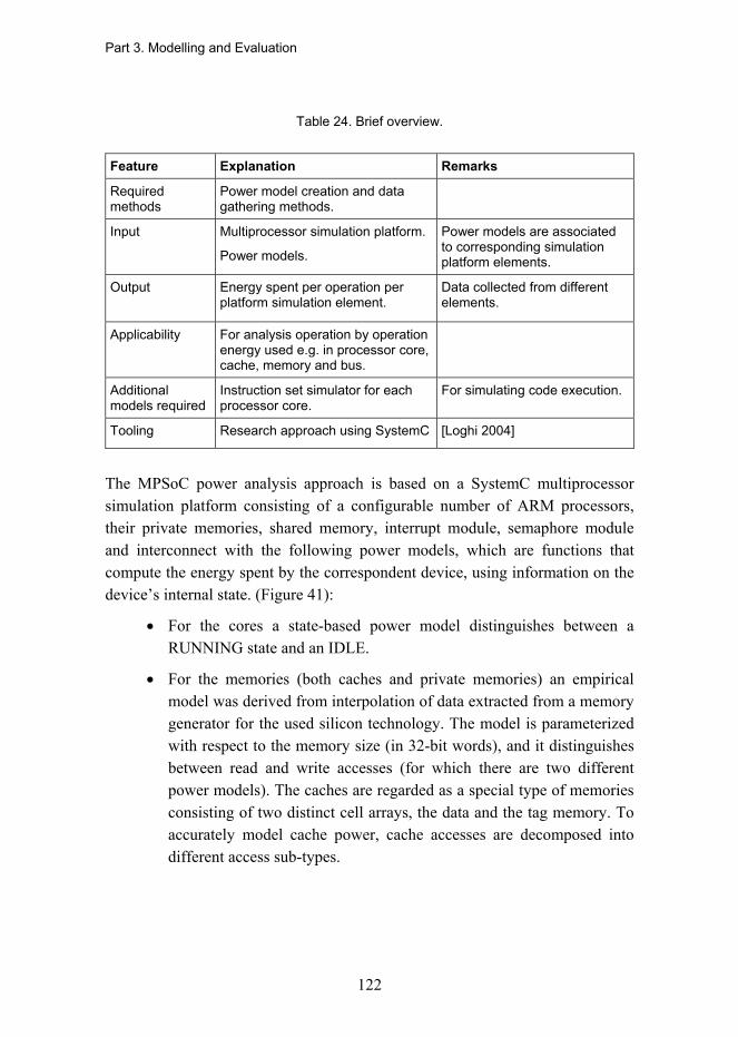
Part 3. Modelling and Evaluation
122
Table 24. Brief overview.
Feature Explanation Remarks
Required methods
Power model creation and data gathering methods.
Input Multiprocessor simulation platform.
Power models.
Power models are associated to corresponding simulation platform elements.
Output Energy spent per operation per platform simulation element.
Data collected from different elements.
Applicability For analysis operation by operation energy used e.g. in processor core, cache, memory and bus.
Additional models required
Instruction set simulator for each processor core.
For simulating code execution.
Tooling Research approach using SystemC [Loghi 2004]
The MPSoC power analysis approach is based on a SystemC multiprocessor simulation platform consisting of a configurable number of ARM processors, their private memories, shared memory, interrupt module, semaphore module and interconnect with the following power models, which are functions that compute the energy spent by the correspondent device, using information on the device�s internal state. (Figure 41):
• For the cores a state-based power model distinguishes between a RUNNING state and an IDLE.
• For the memories (both caches and private memories) an empirical model was derived from interpolation of data extracted from a memory generator for the used silicon technology. The model is parameterized with respect to the memory size (in 32-bit words), and it distinguishes between read and write accesses (for which there are two different power models). The caches are regarded as a special type of memories consisting of two distinct cell arrays, the data and the tag memory. To accurately model cache power, cache accesses are decomposed into different access sub-types.
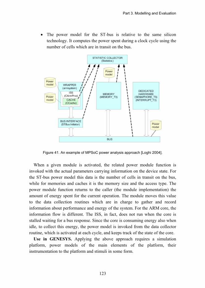
Part 3. Modelling and Evaluation
123
• The power model for the ST-bus is relative to the same silicon technology. It computes the power spent during a clock cycle using the number of cells which are in transit on the bus.
Figure 41. An example of MPSoC power analysis approach [Loghi 2004].
When a given module is activated, the related power module function is invoked with the actual parameters carrying information on the device state. For the ST-bus power model this data is the number of cells in transit on the bus, while for memories and caches it is the memory size and the access type. The power module function returns to the caller (the module implementation) the amount of energy spent for the current operation. The module moves this value to the data collection routines which are in charge to gather and record information about performance and energy of the system. For the ARM core, the information flow is different. The ISS, in fact, does not run when the core is stalled waiting for a bus response. Since the core is consuming energy also when idle, to collect this energy, the power model is invoked from the data collector routine, which is activated at each cycle, and keeps track of the state of the core.
Use in GENESYS. Applying the above approach requires a simulation platform, power models of the main elements of the platform, their instrumentation to the platform and stimuli in some form.
Part 3. Modelling and Evaluation
124
3.8.5 Reliability and Availability Evaluation
Reliability is defined as the probability of the failure-free operation of a system for a specified period of time in a specified environment. Service reliability extends the traditional reliability definition, requiring in turn that either the system does not fail at all for a given period or it successfully recovers state information after a failure for a system to resume its service as if it had not been interrupted. Availability is measured as the probability of a software service or system being available when needed. Reliability and availability are often defined as attributes of dependability, which is �the ability to deliver a service that can justifiably be trusted�. From an architecture point of view, reliability and availability are execution qualities of a system.
In [Goseva-Popstojanova 2001] architecture-based reliability evaluation methods are categorized into state-based, path-based and additive models. All of them are analytical methods. The state-based models use the probabilities of the transfer of control between components to predict the system reliability, whereas the path-based models compute the reliability of composite components based on the possible execution paths of the system. The additive models address the failure intensity of composite components, assuming that the system failure intensity can be calculated from component failure intensities.
Simulation models are used in testing and operational phases [Gokhale 2005]. The aim of simulation is to identify components� criticality to the reliability of an application and detect faults and the number of failures in applications. Thus, simulation models are domain specific and can be regarded as optional approaches in the GENESYS methodology. Monitoring methods use a running system as a source and therefore they are considered only if they give support for architecture-based reliability prediction.
Predicting reliability and availability (RA) from the architectural descriptions is a challenging task for two main reasons:
Reliability is strongly dependent upon how the system will be used. Since reliability and availability are execution qualities, the impact of faults on reliability differs depending on how the system is used, i.e. how often the faulty part of the system is executed. The evaluation of different ways and frequencies to execute the system is a challenge to RA prediction, especially when the usage profiles of the system are unknown beforehand.
The reliability of software architecture depends on the reliability of individual components, component interactions, and the execution environment. The
Part 3. Modelling and Evaluation
125
reliability of a component depends on its internal capabilities, e.g. implementation technology, size, and complexity, information about which might be unavailable, or not yet exist, while architecting. Furthermore, components rely on other components, interactions between components, and on an execution environment, the reliability of which may be unknown.
The GENESYS methodology supports the reliability and availability evaluation by defining methods and techniques that help to consider reliability and availability at three levels: system, architecture and components. Therefore, reliability and availability evaluation is based on the following works: reliability prediction of components based architectures [Reussner 2003] (Table 25), reliability prediction in model-driven development [Rodrigues 2005a] (Table 26), reliability evaluation of service architectures and software families [Immonen 2006] and trustworthiness evaluation and testing of open source components [Palviainen 2008] (Table 27). These approaches have been selected for the starting point based on their contradictory contributions to reliability evaluation concerning the scope of evaluation, modelling languages, abstraction levels, evaluation techniques and tool support. With the exception of the last one, the methods are analytical based on architecture models. The last one is an integrated approach that exploits reliability measurements in order to improve the accuracy of prediction.
3.8.5.1 System Requirements Specification
In order to evaluate reliability and availability, several assumptions are made regarding how quality requirements are specified and how they are mapped to architectural elements. The following sub-sections describe how the RA evaluation is to be considered in the preceding phases of the GENESYS modelling process.
In the System Requirements Specification phase (see Figure 4), the reliability requirements of a system is specified in a way that the information required for reliability evaluation is in the architecture models. The RA evaluation needs the following input from the requirements specification phase:
• Use cases define how different kinds of end-users will use the system. A use case consists of a textual description and a sequence diagram that defines how architectural components interact in the use case.

Part 3. Modelling and Evaluation
126
• A usage profile defines how many times and in which order the use cases occur in a particular usage scenario.
• RA requirements are explicitly defined within the requirement diagrams following the modelling constructs of UML2 and the SysML profile.
Reliability requirements, which are later transformed to RA properties of a system, have the following attributes:
• Quality attribute identifier (string: e.g. RA_id-011)
• Priority class (RA_Pri) (enumerate {high, medium, low})
• Scope of influence (RA_Sco) (enumerate { system | architecture | application | platform | component | service} )
• Metric-ID (string, e.g. M-Re_MTBF), which refers to the reliability metric to be used in the definition of the required, estimated, predicted and measured RA values.
Each RA property has four values:
• RA_target is the RA requirement defined in the system specification phase.
• RA_estimation is based on the heuristic knowledge of a designer and is used only when predicted and measured values are not possible to define.
• RA_prediction is defined by using one of the prediction methods and tools.
• RA_measurement of an existing component/path/system measured by dynamic testing.
The target and measurement values are defined by the Metric_ID metric. The selection of Metric-ID could be supported by the metrics ontology of a particular QA.
Figure 42 introduces an initial taxonomy of reliability metrics [Niemelä 2008]. Because the complete QA metrics ontologies important for GENESYS (i.e. performance and dependability) are not available and the definition of the QA ontologies is out of the scope of GENESYS, the QA metrics are defined in a similar way but without any ontology.

Part 3. Modelling and Evaluation
127
Figure 42. Taxonomy of reliability metrics.
Figure 43 depicts the concepts of QA metrics that can be common for all quality attributes of dependability, whereas only part of the metrics classes and actual metrics in the metrics classes can be shared by different QA ontologies. Each metric has the following properties: purpose; target, i.e. where the metric can be used; applicability, i.e. when the metric can be used; one or more formulas; range value for the measurements; and the optimal value of the measurement. Rules constrain the formulas and used measurement units by defining the set of measurement targets and value ranges and the time when the metric is valid.

Part 3. Modelling and Evaluation
128
Figure 43. Concepts of QA metrics.
In summary,
• QA requirements shall be explicitly defined in the system requirements specification phase. (Criterion: accuracy)
• QA requirements specifications shall be treated as quality properties that are independent of functional requirements.(Criterion: separation of concerns)
• QA requirements shall be defined in a systematic way, i.e. each RA requirement follows the same model. (Criterion: reusability; define once, use every time)
• QA requirements shall be treated as a design artefact of their own. Then their reuse and evolution is possible to manage (Criterion: independence and traceability).
3.8.5.2 Architecture Design
The architecture design phase includes two concurrent activities and an activity where the results of these two activities are combined, refined, and configured in order to meet the system requirements at hand. Here the architecture design phases are considered from a reliability modelling point of view.

Part 3. Modelling and Evaluation
129
Application and platform architecture design
In the architecture design phase, the RA requirements defined in the system requirements specification phase are used for mapping the target RA values to the architectural elements (i.e. components and connectors) of the application architecture. After mapping that is made by the architects, each architectural element affected has an explicit target RA value and a metric for it. The evaluation method to be used depends on the measure the analyzer is interested in. Thus, the architect needs to know which kinds of methods could be used and select the RA value � the metric pair that fits to the method to be used in quality evaluation.
The assumption is that the services provided by the platform module library include the measured or/and estimated RA values. Estimations are made before and after system building.
The electronic reliability prediction methods introduced in [Fuqua 2005] more or less rely on the use of existing reliability data. There is one exception, the system reliability assessment predictive modelling approach that is near to the GENESYS process model including two main parts:
• the system pre-build phases that are supported by the consolidated reliability assessment methodology including phases from requirements specification to manufacturing; and
• the system post-build phases which use e.g. test and process data for predicting the best post-build reliability estimate using Bayesian statistical techniques. The approach is supported by PRISM [PRISM 1999] and FIDES [FIDES 2004] reliability assessment tools.
System Allocation/Configuration/Refinement
In this phase, the application and platform architecture models are combined and a new view, allocation view, is described for deploying software services to computing and communication resources. RA requirements specific for nodes and their connections are added to the allocation view of the system architecture.
Depending on which reliability prediction method is selected, the required input varies. Typically, the state transition diagrams and/or sequence charts have to be annotated by probabilities of state transitions and transactions.

Part 3. Modelling and Evaluation
130
3.8.6 Reliability and Availability Evaluation Methods
Figure 44 depicts the overview of the phase where the reliability and availability of the components, architecture and the whole system are predicted based on analytical models and the measured reliability values of existing components.
Figure 44. Input, output and support for reliability/availability evaluation.
The overview is based on three prediction approaches which will be introduced next. All these approaches are model-driven. Thereafter, a couple of mature commercial tools that support different kinds of analysis are introduced.
3.8.6.1 Reliability Prediction of Component Based Architectures
An overview of the approach is presented in Table 25.

Part 3. Modelling and Evaluation
131
Table 25. Brief overview.
Feature Explanation Remarks
Required methods
A method is based on basic and composite kens (i.e. components at two integration levels) [Reussener 2003].
Applied to component based software architecture of distributed systems.
Input Empirical data, bindings (network connections), mappings (local connections), usage profiles
Empirical data to be obtained by monitoring. If not available to be estimated.
Bindings, mappings and usage profiles to be defined by modelling.
Output Reliability of failure-free operation (MTTF) of basic kens (i.e. components) and composite kens (e.g. sub-system, system).
Measured and predicted reliabilities from an empirical case study; comparison show <1 % deviation.
Applicability Applicable to component based systems but needs to be adapted to UML2 based modelling.
Only one reference, progress not known.
When reliability of required services is < 10%, the precision of the usage profile does not significantly affect the accuracy of the predictions.
Additional models required
Markov chain model. A specific language, RADL (Rich Architectural Description Language).
Tooling Java based test bed constructed for validation.
Contributions
Component reliability. Reliability is predicted for basic kens and composite kens. For basic kens the provided and required gates (including protocol Finite State Machine (FSM)) and the service FSM usage profile of provided services are modelled. The last one extends a service FSM to a Markov chain model. To link reliability of the required gates to the reliability of services in the provided gates, the parameterised contracts combine the service FSM usage profile and the reliabilities of required interfaces to compute the missing reliabilities for the external services. Finally, the overall reliability of a ken is calculated.
Part 3. Modelling and Evaluation
132
Similar to basic kens the reliability of composite kens is calculated in two phases; first the service reliability and then the overall reliability. Equations for calculations are presented in [Reussener 2003].
Limitations
The method requires the following input data:
1) For basic kens (considered as black box components) the service effect FSM and a usage profile from a vendor and the required services reliability from a buyer.
2) For composite kens (considered as gray boxes, assembly) the service effect FSM of inner basic kens, binding and mapping reliabilities form a vendor and the required services reliability from a buyer.
Use in GENESYS
Application of this method in GENESYS requires the following adaptations:
• To be adapted to UML2 � MARTE modelling language
• Tool support for automating the definition of the Markov chain model and parameterized contracts
• No recent publications that would help.
3.8.6.2 Reliability Evaluation in Model Driven Development
An overview of the approach is presented in Table 26.

Part 3. Modelling and Evaluation
133
Table 26. Brief Overview.
Feature Explanation Remarks
Required methods
Reliability prediction method [Rodriques 2005a], Sensitivity analysis method [Rodriques 2005b].
Applied to software systems.
Input Scenarios as a collection of Basic Message Sequence Charts (BMSC) and High-Level Message Sequence Charts (HMSC).
Operational profile.
BMSC describes message exchange between components. HMSC provides sequential, conditional and iterative composition of BMSCs.
Output System�s reliability, implied scenarios and sensitivity of the system reliability.
Reliability value (0�1).
Implied scenario = a system produces a trace that reveals a mismatch between behaviour defined in architecture.
Sensitivity to changes in individual probability values.
Applicability System and architecture level reliability prediction based on models. Active work around the topic.
Answers to the following questions:
Is there any implied scenario in the system architecture model?
What is the impact of implied scenarios on reliability?
Is reliability change sensitive?
Additional models required
A specific reliability prediction profile.
The profile required for annotating scenarios.
Tooling LTSA, from UML to LTSA transformation.
LTSA as an Eclipse plug-in http://www.doc.ic.ac.uk/ltsa/eclipse/
XSLT used for transforming the XMI form of the UML model to XML input for LTSA.

Part 3. Modelling and Evaluation
134
Contributions
System reliability prediction as part of model-driven development. The method includes the following steps:
• Scenario specification by annotating (high and basic) message sequence charts by using a specific reliability profile.
• A probabilistic Labelled Transition System (LTS) is synthesised from the annotated scenarios. Mapping of the probability annotations of the scenario specification into probability weights for transitions in the synthesised architecture model.
• The synthesised architecture model is interpreted as a Markov model by applying Cheung�s reliability prediction method extended by one initial and one final scenario.
• Performing sensitivity analysis of the prediction.
• LTSA has the following extensions: • LTSA-UML which allows models to be described by UML2-XMI and
translates UML2 interaction models to be translated to message sequence charts.
• LTSA-MSC which allows models to be described by graphically editing sets of scenarios in the form of message sequence charts (MSC). The LTSA can be used to detect the presence of implied scenarios in the system as part of an iterative design process.
• LTSA WS-Engineer which allows service models to be described by translation of the service process descriptions, and can be used to perform model-based verification of web service compositions.
Limitations
An HMSC in LTSA cannot have multiple nodes that correspond to the same BMSC. LTSA does not support hierarchically-nested HMSCs.
Use in GENESYS
This method could be adopted quite easily for GENESYS due to support for UML2 based modelling and evaluation tools.
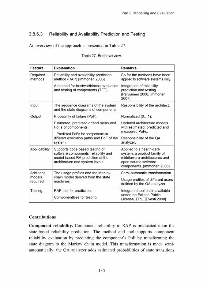
Part 3. Modelling and Evaluation
135
3.8.6.3 Reliability and Availability Prediction and Testing
An overview of the approach is presented in Table 27.
Table 27. Brief overview.
Feature Explanation Remarks
Required methods
Reliability and availability prediction method (RAP) [Immonen 2006].
A method for trustworthiness evaluation and testing of components (TET).
So far the methods have been applied to software systems only.
Integration of reliability prediction and testing [Palviainen 2008, Immonen 2007].
Input The sequence diagrams of the system and the state diagrams of components.
Responsibility of the architect.
Output Probability of failure (PoF).
Estimated, predicted or/and measured PoFs of components.
�Predicted PoFs for components in different execution paths and PoF of the system.
Normalized (0�1).
Updated architecture models with estimated, predicted and measured PoFs.
Responsibility of the QA analyzer.
Applicability Supports code based testing of software components� reliability and model-based RA prediction at the architecture and system levels.
Applied to a health-care system, a product family of middleware architectures and open source software components. [Immonen 2008]
Additional models required
The usage profiles and the Markov chain model derived from the state machines.
Semi-automatic transformation.
Usage profiles of different users defined by the QA analyzer.
Tooling RAP tool for prediction.
ComponentBee for testing.
Integrated tool chain available under the Eclipse Public License, EPL. [Evesti 2008]
Contributions
Component reliability. Component reliability in RAP is predicated upon the state-based reliability prediction. The method and tool supports component reliability evaluation by predicting the component�s PoF by transforming the state diagram to the Markov chain model. This transformation is made semi-automatically; the QA analyzer adds estimated probabilities of state transitions
Part 3. Modelling and Evaluation
136
and the PoF of each state; the tool adds a separate failure state and calculates new probabilities for state transitions and finally the predicted PoF for the component.
The ComponentBee tool is used for calculating the measured PoF of components. The tool requires a component-specific test model, which is derived from the usage profile of the system and a set of sequence diagrams that describe the architectural components in different scenarios. ComponentBee provides plug-ins for recording raw and trace data and calculating the measured PoF of a component from the extracted behaviour patterns.
System/architecture reliability. Architecture-level reliability and availability prediction is a path-based approach. As input it requires a behaviour model (i.e. sequence diagrams) of the architecture and the usage profiles of the system. As output it gives a predicted PoF value for each execution path and the predicted PoF value for the whole system. Calculation of the PoFs for execution paths is made separately and is based on the components� PoF values and probabilities of transitions in the execution paths. By analysing the reliabilities of execution paths and the components reliabilities involved in a particular path, the reliability sensitivity points of the architecture can be identified. The execution order of the paths has no impact on the system level reliability.
Limitations. The approach has been applied only to software systems. The accuracy of the system�s PoF depends on accuracy of the predicted PoFs of components. Thus, the measured PoFs of existing components increase the accuracy of the system PoF value. Although the recent version of the ComponentBee supports only Java components, the approach might be adapted to the components of embedded systems that include software and hardware.
Use in GENESYS
Use of the RAP tool is quite straightforward but needs adaptation to the components of embedded systems. ComponentBee supports only Java components and requires the test bed that means application specific implementation.
3.8.6.4 Commercial Reliability Analysis Tools
Reliability Workbench is Isograph�s flagship suite of Reliability Analysis software [Isograph 2008]. This tool supports many kind of analysis: reliability and maintainability prediction, failure mode effect and criticality analysis (FMECA), reliability block diagram analysis, reliability allocation, fault tree
Part 3. Modelling and Evaluation
137
analysis, event tree analysis and Markov analysis. The use of the tool allows for predicting a system�s reliability, identifying the critical components of a system and finding out which design changes will improve the system reliability and estimating the consequences and risks of system failures. The tool is stand alone and each module requires specific input information (i.e. it is not UML compatible). The problem is the same with ReliaSoft�s Lambda Predict tool that supports all major prediction standards [ReliaSoft 2008]. The maturity of these tools is obvious. However, the goal of GENESYS is to support the whole life-cycle of model driven development of embedded systems and therefore, the use of these tools requires remarkable adaptation work in order to make them able to interoperate with UML2 modelling tools in the Eclipse environment. Moreover, experience of applying these tools in a specific domain area should be gained before starting the adaptation.
3.8.7 Safety Analysis
A safety critical system is a system in which an action incidence (not performed, or performed incorrectly in logic or in time), could result in danger, injury, death, or property damages. An intrinsically safe system, on the other hand, cannot cause harmful exposures or damage under normal or abnormal conditions even when the equipment and personnel are in their most vulnerable condition [Leveson 1991, Leveson 1995].
Safety properties are normally defined by using two factors: hazard and its risk. Hazard is a system state potentially causing accidents while the risk is concerned with the degree of acceptance of the hazard in certain environmental conditions, determined by severity, probability, exposure time, operation modes and possible mitigation of the hazard�s effect.
A safety assessment process provides analytic evidence showing compliance with system requirements. The process includes specific assessments conducted and updated during system development; both processes interact along the product life-cycle. General safety assessment processes are structured as follows: [EMMA 2005]
• Functional Hazard Assessment (FHA): Examines system functionalities to identify potential functional failures, classifies the hazards associated with specific failure conditions and severity, and assigns safety objectives to the failure conditions of the functions. The FHA is

Part 3. Modelling and Evaluation
138
performed early in the development process and is updated as new functions or fault conditions are identified. The applicable method is:
o PHA (Preliminary Hazard Analysis). • Preliminary System Safety Assessment (PSSA): Establishes specific
system and item safety requirements and provides a preliminary indication that the anticipated system architecture can meet those safety requirements. The PSSA is updated throughout the system development process. It is also used to ensure completeness of the failure conditions list from the FHA. All safety requirements should be traceable from the PSSA to the system requirements. The applicable methods are:
o Failure Modes, Effects (and Criticality) Analysis (FME(C)A) o Failure Effects Summary (FES) o Fault Tree Analysis (FTA) that can be performed at several
levels. • System Safety Assessment (SSA): Collects, analyses, and documents
verification that the system, as implemented, meets the system safety requirements established at analysis time. It uses the same applicable methods as PSSA.
• Common Cause Analysis (CCA): Establishes and validates physical and functional separation and isolation requirements between systems and verifies that these requirements have been met. The applicable methods are:
• Zonal Safety Analysis (ZSA), Particular Risk Analysis (PRA), and Common Mode Analysis (CMA).From the point of view of safety-related systems, it is usual to define a life cycle where both the course of development and safety management of the system are realized in parallel.
3.8.7.1 Safety Analysis Techniques
Figure 45 gives an overview of the safety analysis techniques that are introduced next.

Part 3. Modelling and Evaluation
139
Figure 45. Taxonomy of safety analysis techniques.
Classical Safety Analysis Techniques
Safety analysis is performed according to an industrial domain-specific standardized process (see IEC-61508, NASA-STD-8719.13A, WD 26262 and MIL_STD_882), addressing two major tasks: risk assessment and hazard analysis.
The aim of risk assessment is to determine acceptance criteria of hazards especially when it is assumed such hazards could not be completely avoided. This is normally performed by considering the environmental conditions along with the exposure or duration factors. A risk can be defined as the combination of the hazard-level, the likelihood of accident, and hazard exposure/duration. Risk can also be defined as a function of the frequency of occurrence of an undesired event, the potential severity of consequences, and the uncertainties associated with its frequency and severity.
Hazard analysis aims to identify hazards as well as their causes and consequences, to assess the levels of hazards in terms of probability and criticality, and finally, to derive safety specific requirements or approaches (e.g.

Part 3. Modelling and Evaluation
140
architecture, patterns, etc). For safety critical systems, this analysis is performed at different design stages and with different levels of abstraction.
A general approach is to apply PHA (Preliminary Hazard Analysis) aligned to system requirement analysis. This identifies all the undesired events linked to the studied system, classifies them regarding severity and probability criteria, selects the most critical of them that will be the subject of further detailed assessment and determines specific safety requirements for the system. Further steps consist on applying FAA (Functional Failure Analysis) at system-level for the analysis of top-level hazards and FMEA (Failure Modes and Effects Analysis) [Kletz1992] at the subsystems/components for the derivation of causes. The different results are usually captured in tabular form.
Fault tree analysis (FTA) is a top-down failure analysis in which an undesired state of a system is analyzed using boolean logic to combine a series of lower-level events, which determines the probability of a safety hazard as fault trees depicting the causal or logical relationships of events.
Other techniques can be used at different stages of the development, in a complementary way: SHA (System Hazard Analysis � System Requirement Analysis), SSHA (Subsystem Hazard Analysis � Subsystem Requirement Analysis) or OSHA (Operating and Support Hazard Analysis � System Requirement Analysis) [FAA2008].
Extensions to the traditional techniques are defined for software safety management; this way, SFTA (Software Fault Trees Analysis) for software programs provides a failure semantics for the elements of a programming language or detailed design to support the reasoning of logical errors to show that a specific software design will not produce system safety failure. Failing that, it determines the environmental conditions that could lead it to cause such a failure� [Rushby1993]. SFMEA is a table-based design analysis technique which determines system effects of each failure mode of every software component, identifies and traces failures leading to specific events.
Model-based Safety Analysis
Traditional analysis techniques, introduced above, are based on information synthesized from several sources, including informal design models and requirements documents. This circumstance determines a major pitfall; they are highly subjective and dependent on the skill of the engineer. Even after a consensus is reached, it is unlikely that the analysis results will be complete, consistent, and error free due in part to the informal models used as the basis of

Part 3. Modelling and Evaluation
141
the analysis. In fact, the lack of precise models of the system architecture and its failure modes often forces the safety analysts to devote much of their effort to gathering information about the system architecture and system behaviour and embedding this information in the safety artefacts such as the fault trees. The use of safety analysis activities based on formal/semi-formal models of the system under development significantly improves this obstacle; the extension of the model-based development to incorporate the safety analysis activities in addition to the traditional development activities.
A model-based approach has several benefits when integrated into safety analysis processes:
• Integration between systems and safety analysis is based on common models of system architecture and failure modes.
• Simulation of the behaviour of system architectures occurs early in the development process to explore potential safety hazards.
• Exploration all possible behaviours of a system architecture is exhaustive with respect to some safety property of interest using automated analysis tools.
• Generation many of the artefacts that are manually created during a traditional safety analysis such as fault trees and FMEA/FMECA charts or formal demonstration of compliance of the requirements or the finding of counter-examples as exception to the desired behaviour is automatic.
The methodology framework considers the errors and failures at different levels of abstraction and integration (e.g. system-level, device-level or chip-level). Once extended to the system model and defined according to the behaviour of the system, the safety analysis task involves verifying whether safety requirements keeps on the occurrence of the faults previously defined in the fault model. Here, numerous approaches have been developed [Joshi 2005]; to perform exploratory analysis by simulating faults on specific components and observing the behaviour of the system or more rigorous analyses, it is possible to use formal verification tools to determine whether safety properties of interest hold. This criteria determines the main approaches.

Part 3. Modelling and Evaluation
142
Simulation
Having a formal model of the system extended with the fault model enables the engineer to simulate different failure scenarios as exploration of �what-if� scenarios involving combinations of faults through simulations.
This provides engineers with the facility of visualizing in a interactive way, the effect of faults on system functionality. This capability can be used as a preliminary analysis, to quickly detect safety problems in common scenarios before performing a more rigorous static or dynamic analysis.
Failure Logic Modelling (FLM)
This approach emerged from the observation that traditional analysis methods do not yield reusable models; after any modification, the whole range of analysis models must be reviewed and recalculated. The FLM techniques, follow a component-based approach for certification and allow modelling of the failure behaviour of the system in an incremental fashion as design work progresses from system architecture to a detailed level. It breaks down the system-level assessment, which would otherwise be very complex, into more manageable tasks of characterisation of failure behaviour of individual components. With adequate tool support, the analysis results could be represented in the form of familiar safety artefacts (such as Fault Trees or FMEA tables), automatically extracted from the failure logic model, with the guarantee of consistency between views.
Formal Methods (FM)
Formal verification tools, such as model checkers and theorem provers, can be used to prove that a safety property holds over the extended system model. To prove interesting properties, an engineer will typically have to rule out certain unlikely combinations of failures. These can be encoded as assumptions or axioms that will be used in the proof process. If a property is proved, then the responsibility of the safety engineer is to review the assumptions that were used in the proof and check whether they are realistic. If so, the engineers have a mathematical proof that the system satisfies the safety property with respect to the fault model. In case a property is not proved, it may be necessary to re-architect the system or to relax the original safety property to accommodate delay or other acceptable constraints to allow system recovery. Some techniques are available:

Part 3. Modelling and Evaluation
143
Model checking Approach. Given a description of a system in some formal notation and a list of properties that must hold of the system, the inference system verifies whether the property is true, or the property is false with a counter example; does not generate results in the form of traditional safety artefacts, like fault trees. Different variants are currently evaluated: SPIN [Baier 2008, Holzmann 2003], BDD (Binary Decision Diagrams), SAT (Satisfiability Tecnhnique) and others [ESACS 2004].
Theorem Proving Approach. Theorem proving is another method for performing verification on formal specifications of system models. Theorem provers (for example, PVS, http://pvs.csl.sri.com) verify or apply rules of inference to a specification in order to derive new properties of interest. Rather than exploring the global state space, theorem provers automate human reasoning, reducing a proof goal (with human guidance) to simpler sub-goals that can be discharged automatically by the primitive axioms or decision procedures of the prover.
Constraint Satisfaction Approach. Error and failure behaviour are composed as a network of relations and the problems described by such networks are referred to as Constraint Satisfaction Problems (CSP). CSPs are networks of variables interconnected by a set of relations called constraints [Tsang 1993]. A CSP is solved, if a value assignment has been found for all variables, such that all the relations are satisfied. Constraints have several interesting properties [Barták 2001]; like a constraint does not need a unique specification of all the values of its variables thus they may specify partial information which can be exploited using on-the-fly diagnosis procedures. Constraints are non-directional, declarative (they specify what relationship must hold without specifying a computational procedure to enforce that relationship), additive (the conjunction of constraints is effective independently of the order of imposition of constraints), and compositional, as hierarchical refinement is supported. The use of relations in CSPs provides proper support for handling non deterministic abstractions of complex systems [Pataricza 2006].
3.8.7.2 GENESYS Safety Certification Approach
The inherent properties of the cross-domain architectural style and its domain specific instantiations, allow a modular certification approach (Figure 46). For the instantiated systems (aligned with the cross-domain architectural style and reference architecture template), the overall system can be subdivided into

Part 3. Modelling and Evaluation
144
subsystems with different levels of criticality; each of them can then be individually certified to the appropriate level of criticality, avoiding the full product certification to the highest criticality level of all subsystems, reducing cost and simplifying the complexity of certification effort [Obermaisser 2005].
This process is supported by the definition of Modular Safety Cases [Kelly 1999, Kelly 2003] and provides an independent certification of platform service from applications and management of independent safety arguments for different functions:
• Separating certification of architectural services from applications. The certification of the overall system is supported by a baseline formed by the certified architectural services [Nicholson 2000, Obermaisser 2005].
• Separating certification of different functionalities. Instead of considering the system as a monolithic block; the certification will be accomplished incrementally.
Figure 46. Modular application safety case for GENESYS product.
Within GENESYS safety certification, the main focus is the support by realization of early model-based FHA and PSSA and the provision of artefacts such as fault trees and FMEAs automatically generated as product of the quality analyses. Figure 47 shows the relation and link between the GENESYS methodology and safety assessment process.
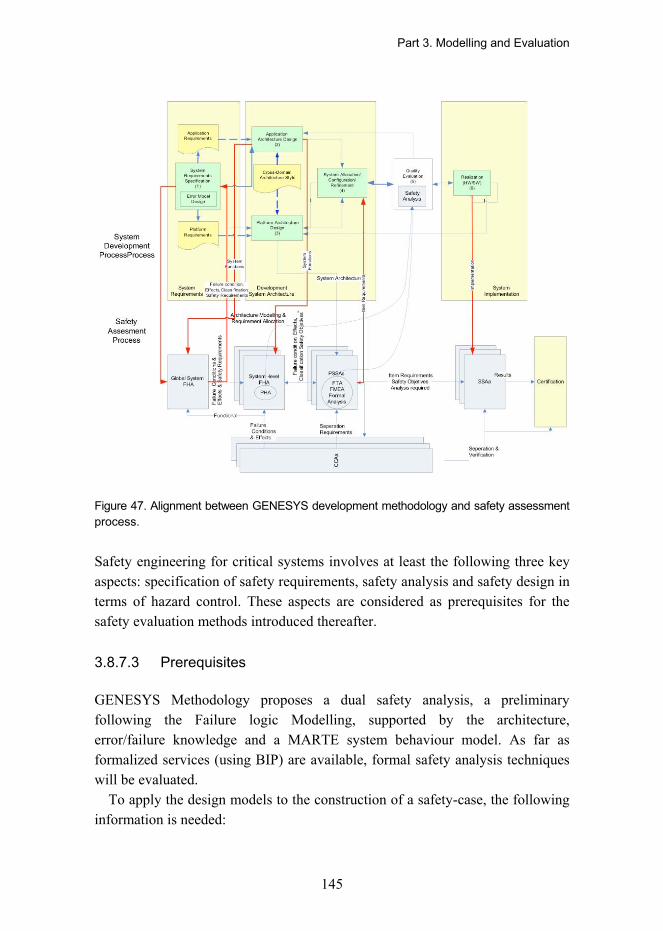
Part 3. Modelling and Evaluation
145
Figure 47. Alignment between GENESYS development methodology and safety assessment process.
Safety engineering for critical systems involves at least the following three key aspects: specification of safety requirements, safety analysis and safety design in terms of hazard control. These aspects are considered as prerequisites for the safety evaluation methods introduced thereafter.
3.8.7.3 Prerequisites
GENESYS Methodology proposes a dual safety analysis, a preliminary following the Failure logic Modelling, supported by the architecture, error/failure knowledge and a MARTE system behaviour model. As far as formalized services (using BIP) are available, formal safety analysis techniques will be evaluated.
To apply the design models to the construction of a safety-case, the following information is needed:

Part 3. Modelling and Evaluation
146
• Safety Requirements. Specific safety-related requirements elicited from the preliminary safety analysis and safety integration labelled according to the functional requirements of the system.
• Architecture. A model of the system architecture, describing the different blocks, components and elements which constitute the system to be analyzed. See point 6.5. Platform Architecture Design).
• Behaviour. Since the safety analysis requires knowledge of the different faults that can occur and the various ways in which the system components can malfunction, the proposed nominal (non-failure) system behaviour (see point 6.4.3. Behaviour View) captured must be augmented with the fault behaviour of the system to create the Extended System Model [Leveson 2000].
• Hazards, failures and faults. The following concepts are specified and modeled.
- hypotheses of defects � expressed solely in terms of the system � must be provided to avoid mistaking fail-safe behaviour of the model for fail-safe behaviour of the system.
- characterisation of failures � expressed solely in terms of the interface between system and environment � must be provided to allow identifying deviations from the intended behaviour in the interaction between the system and its environment.
- identification of hazardous situations � expressed solely in terms of the environment � must be provided to allow describing hazards in terms of the controlled environment rather than the controlling system.
3.8.7.4 System Requirements Specification
The objectives of the PHA analysis are to identify all the undesired events linked to the studied system, to classify them regarding severity and probability criteria, and to select the most critical of them that will be the subject of further detailed assessment. The levels of hazards indicate the necessities of safety-related design; high level hazards need to be treated either by making changes in the design, by mitigating the severity of hazard by safety devices, or by reducing the likelihood of hazards using architectural approaches. The specifications of such
Part 3. Modelling and Evaluation
147
measures in terms of related design criteria and constraints are referred to as safety requirements.
Closely related to the concept of safety design requirements are the Safety Integrity Levels (SILs), which introduces the following concepts [IEC-61508]:
• Risk: a measure of the severity and probability of dangerous failures.
• Safety functions: E/E/PES systems and other technologies that are introduced in order to achieve functional safety, i.e., to maintain the risks at acceptable levels in respect of hazardous events.
• Safety function requirements: relating to the functionality of a safety function, derived from hazard analysis.
• Safety integrity requirements: relating to the effectiveness of a safety function in terms of its likelihood of performing satisfactorily, determined based on risk assessment.
The derived safety / safety integrity requirements are annexed to functional and non-functional requirements and managed during the system life cycle. In support automated analysis, the safety properties must be expressed using some formal notation.
Depending of the general approach, there are several candidate notations:
• For an FLM solution, the safety integrability requirements are specified by labelling the jobs at different integration and abstraction levels with corresponding SIL, according to the specific safety norm (IEC-61508, DW 26262, �). Here, there is no common terminology, values and semantics although similar are domain-specific so MARTE does not provides specific NFP types, for the specification of the set of qualified values required to precisely specify and qualify an SIL attribute.
• An additional attribute to <<RtUnit>> stereotype, silLevel: NFP_String [1] should be provided.
Related to a formal approach, the requirement model is based on temporal logics like CTL/LTL [Gabbay 1994, Baier 2008] or higher order predicate logics [Andrews 2002]. Temporal logic formulas are boolean expressions with additional operators to express properties over time. Representative samples are NuSMV or SCADE SPPI [ESACS 2004].

Part 3. Modelling and Evaluation
148
3.8.7.5 Fault and Hazard Modelling
Error modelling provides a capture if potential errors, failure behaviour and propagation, providing a complementary extension of the nominal to support the system safety and dependability analysis. Some concepts are involved: a failure is an inability of a system to perform its required functions within specified performance requirements. [IEEE 610.12-1990]. The deviation from correct behaviour (nominal) may assume different forms that are called service failure modes. The adjudged or hypothesized cause of an error is called a fault. In most cases, a fault first causes an error in the functional state of a component that is a part of the internal state of the system and the external state is not immediately affected. The definition of an error is the part of the total state of the system that may lead to its subsequent system failure.
The component failure will be triggered by some internal or propagated fault. In order to trigger these faults, we add additional inputs to the extended model for each fault that can occur within a component in the nominal model. A fault model should contain:
1. component failure mode behaviour specifications,
2. additional inputs for activating faults a. intrinsic faults activated through system level inputs, and b. propagated faults activated by the error propagating component.
Three different levels of resolution are possible [Pataricza 2006]:
1. Static, error and fault dependability assessment models describe the signal flow in a system mapping them to a single attribute of failure mode. The set of failure modes contains in the simplest case of pass/fail categorization only the values of good and faulty. In the case of a more detailed modelling, the faulty case is refined into multiple values according to failure modes.
The core idea of fault level analysis is the characterization of the sensitivity of the individual components in the system by means of relations between the error manifestations at their inputs and outputs. It serves as an early check of the appropriateness of the dependability concept, thus avoiding extremely costly redesign cycles due to violations of dependability requirements.
Part 3. Modelling and Evaluation
149
2. Another option, dynamic error propagation analysis deals with the dynamics of propagation of discrepancies appearing as fault impacts in a system. This is done both by an intuitive method creating the basic models heuristically and by an algorithm automatically deriving them from the functional description of the components.
Abstract dynamic error propagation analysis relies on a model of the dynamics of the target system (internal operation sequences in the components, their mutual interaction and invocation) in order to incorporate the activation sequences into the analysis.
The introduction of error modes as a main representation facilitates the creation of a simple automaton describing the impacts of errors appearing at inputs of the individual components (p.e. timed failure propagation graphs (TFPG) [Abdelwahed 2006]).
3. Finally, the foundations of model transformation generating formal analysis models from engineering ones are addressed (See. Formal Methods approach).
The GENESYS methodology approach, considers the errors and failures at different levels of abstraction and integration (e.g. system-level, device-level or chip-level).
Different formalism (formal/semi-formal, static-dynamical) has been proposed for the error behaviour and propagation modelling at each level. EAST-ADL2 is an architecture description language, dedicated to automotive embedded electronic systems, developed in the context of the ITEA cooperative project EAST-EEA (http://www.easteea.net/) and ATESST project (www.atesst.org); extending UML2 standard and addressing the new automotive domain standardization AUTOSAR (http:// www.autosar.org/) represents error propagations and emphasizes either the temporal aspect or the causal aspects (Figure 48).
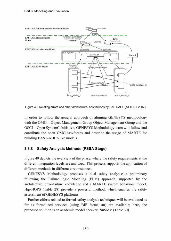
Part 3. Modelling and Evaluation
150
Figure 48. Relating errors and other architectural abstractions by EAST-ADL (ATTEST 2007).
In order to follow the general approach of aligning GENESYS methodology with the OMG � Object Management Group Object Management Group and the OSCI � Open SystemC Initiative, GENESYS Methodology team will follow and contribute the open OMG taskforces and describe the usage of MARTE for building EAST-ADL2-like models.
3.8.8 Safety Analysis Methods (PSSA Stage)
Figure 49 depicts the overview of the phase, where the safety requirements at the different integration levels are analyzed. This process supports the application of different methods in different circumstances.
GENESYS Methodology proposes a dual safety analysis: a preliminary following the Failure logic Modeling (FLM) approach, supported by the architecture, error/failure knowledge and a MARTE system behaviour model. Hip-HOPS (Table 28) provide a powerful method, which enables the safety assessment of GENESYS platforms.
Further efforts related to formal safety analysis techniques will be evaluated as far as formalized services (using BIP formalism) are available; here, the proposed solution is an academic model checker, NuSMV (Table 30).
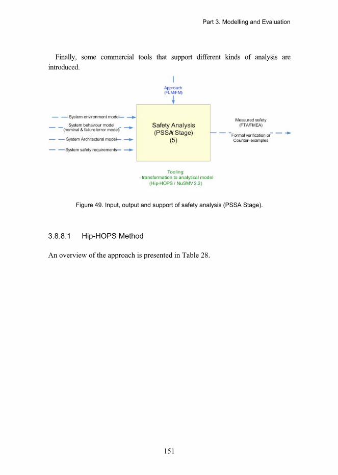
Part 3. Modelling and Evaluation
151
Finally, some commercial tools that support different kinds of analysis are introduced.
Figure 49. Input, output and support of safety analysis (PSSA Stage).
3.8.8.1 Hip-HOPS Method
An overview of the approach is presented in Table 28.

Part 3. Modelling and Evaluation
152
Table 28. Brief Overview.
Feature Explanation Remarks
Required methods
HiP-HOPS (Hierarchically Performed Hazard Origin and Propagation Studies) [Papadopoulos 1999].
Integrated assessment of hierarchically described system at different levels of detail: from functional level to lower HS/SW design level.
Input Function block and failures, effects, severity information.
Error behaviour and propagation.
Description of a topology of a system model (hierarchical if necessary to manage complexity) that includes information about component failures and their local effects.
Output System�s reliability, implied scenarios and sensitivity of the system reliability.
Modify and incorporate classical techniques and generates the following information in an incremental way:
• Early: FFA+ (Extended FFA)
• Later: IF-FMEA (Interface Focused FMEA)
• Across: FTA (Mechanically generated).
Applicability System and architecture level safety analysis based on models. Current research topic.
Answers to the following questions:
Which risk has the greatest concern, and therefore an action is needed to prevent a problem before it arises?
Which are the probabilities of system failure?
Additional models required
A specific error management profile. Solution: EAST-ADL profile (annex A. of MARTE profile specification).
The profile required for modelling the information related to errors (behaviour, propagation, etc).
Tooling HiP-HOPS (University of York under commercialization process).
HiP-HOPs as an isolated tool.
Part 3. Modelling and Evaluation
153
Contributions
This method aims to enable an integrated safety analysis from abstract functional level to low level component failure modes based on a hierarchical system description. The analysis process starts from an FFA analysis and produces a hierarchical system model in which possible system hazards are identified. Failure behaviours of components in this model are then further analyzed considering both the local failures of an individual component and its reactions to failures caused by other components. Finally, HiP-HOPS performs a fault-tree synthesis determining faults propagation in the entire system. The integration is based on a neutral format of input for HiP-HOPS in a �.hip�, allowing the development of interface to HiP-HOPS, In all instances, HiP-HOP currently supports Matlab/Simulink model analysis by using a toolbox which produces failure-modes annotation and the required failure data.
The harmonization of HiP-HOPs with EAST-ADL2 is more aligned with the primary modelling approach of the methodology framework, which is an Architecture Description Language developed by ATESST, a consortium of universities and automotive companies in a project directly funded by the consortium. The ATESST approach supports safety analysis by providing a hierarchical system analysis model that consists of failure semantics at each abstraction level. Table 29 explains the mapping between concepts between EAST-ADL2 and the HiPHOPS. The implementation is performed using EMF (Eclipse Modeling Framework) APIs and Eclipse UML2 APIs.

Part 3. Modelling and Evaluation
154
Table 29. EAST-ADL2 and HiP-HOPS concepts for safety analysis [ATESST 2007].
GENESYS Concepts Explanation HiP-HOPS Concepts
FunctionType It represents basic entities.
Function Prototype / FunctionalDevice
these two are specializations of FunctionalType. Abstraction Function
ErrorBehavior
It defines the Specification of error logic. Properties such failure logic, propagation port, handling status and failure effects.
Functions failures, effects, severity. Component failures.
ErrorModel
It defines the ErrorBehavior that a entity can have given a specific context.
Implementation of a component that allows synthesis and analysis to take place.
ErrorPropagation
It defines the relationships between errors of components which can cross abstraction levels.
Propagation of failure and faults.
PropagationPort It defines the port that an faulty event can go through. Failure data port.
Safety analysis as part of model driven development. The method includes the following steps:
1. Scenario specification, defining the operational environment by fault behavioural modelling. By using EAST-ADL2 profile.
2. Construct a function block diagram, which identifies system functions and their dependencies. Output from Platform Architecture Design stage.
3. Assess multiple functional failures (FTA, FMEA).
Limitations. The component behaviour is not considered while generating the fault trees; there is no fault order dependency information, which is important or necessary in a system under synchronization requirements.
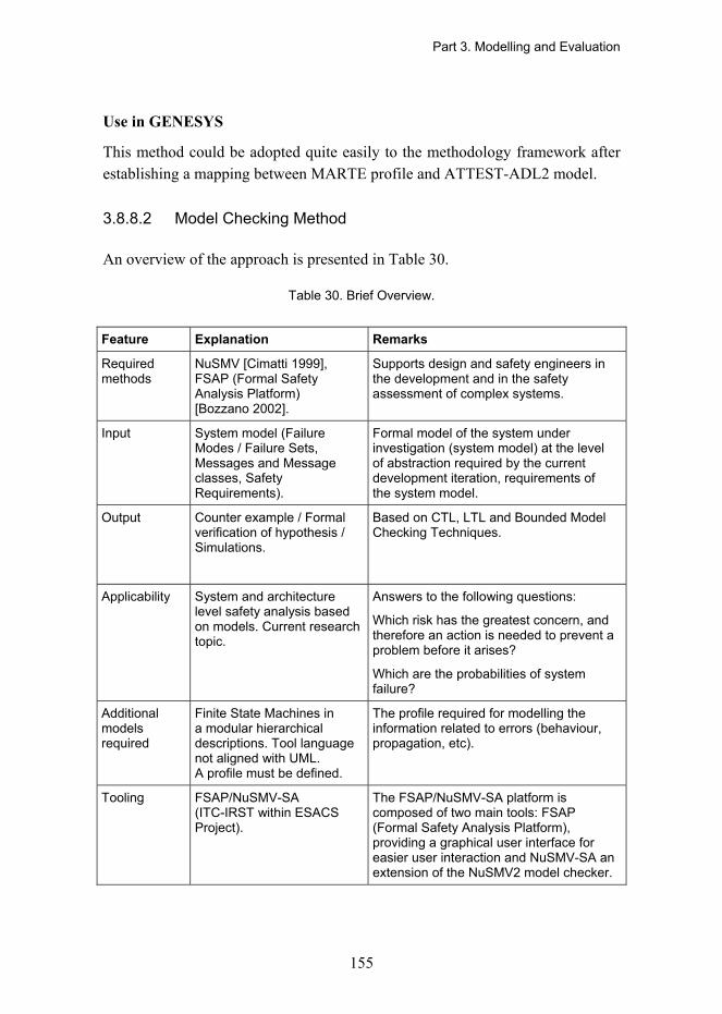
Part 3. Modelling and Evaluation
155
Use in GENESYS
This method could be adopted quite easily to the methodology framework after establishing a mapping between MARTE profile and ATTEST-ADL2 model.
3.8.8.2 Model Checking Method
An overview of the approach is presented in Table 30.
Table 30. Brief Overview.
Feature Explanation Remarks
Required methods
NuSMV [Cimatti 1999], FSAP (Formal Safety Analysis Platform) [Bozzano 2002].
Supports design and safety engineers in the development and in the safety assessment of complex systems.
Input System model (Failure Modes / Failure Sets, Messages and Message classes, Safety Requirements).
Formal model of the system under investigation (system model) at the level of abstraction required by the current development iteration, requirements of the system model.
Output Counter example / Formal verification of hypothesis / Simulations.
Based on CTL, LTL and Bounded Model Checking Techniques.
Applicability System and architecture level safety analysis based on models. Current research topic.
Answers to the following questions:
Which risk has the greatest concern, and therefore an action is needed to prevent a problem before it arises?
Which are the probabilities of system failure?
Additional models required
Finite State Machines in a modular hierarchical descriptions. Tool language not aligned with UML. A profile must be defined.
The profile required for modelling the information related to errors (behaviour, propagation, etc).
Tooling FSAP/NuSMV-SA (ITC-IRST within ESACS Project).
The FSAP/NuSMV-SA platform is composed of two main tools: FSAP (Formal Safety Analysis Platform), providing a graphical user interface for easier user interaction and NuSMV-SA an extension of the NuSMV2 model checker.

Part 3. Modelling and Evaluation
156
Contributions
NuSMV has been developed as a joint project between ITC-IRST (Istituto Trentino di Cultura, Istituto per la Ricerca Scientifica e Tecnologica in Trento, Italy), Carnegie Mellon University, the University of Genoa and the University of Trento. It is a reimplementation and extension of SMV, the first model checker based on Binary Decision Diagrams (BDDs). The tool has been designed as an open architecture for model checking. It is aimed at reliable verification of industrially-sized designs, for use as a backend for other verification tools and as a research tool for formal verification techniques.
The FSAP/NuSMV-SA platform aims at supporting the formal analysis and safety assessment of (complex) systems. The platform is based on a set of tools (including an extension of the NuSMV model checker) and is based on the concept of a repository. The repository contains the information necessary for the design and safety assessment of systems and is shared between the design engineer (the actor responsible for the design of the complex system) and the safety engineer (the actor responsible for performing safety analysis on the complex system).
The platform is designed to support different phases of the development and safety assessment process and to support different development and safety assessment practices. To achieve these goals, FSAP/NuSMV-SA provides a set of basic functions. These basic functions can be combined in different ways to perform complex tasks. The major benefits from the use of FSAP/NuSMV-SA are the following:
• The platform supports a tight integration between the design and the safety teams
• The platform automates (some of) the activities related both to the verification and to the safety analysis of systems in a uniform environment
• The use of the platform is compatible with an incremental development approach, based on iterative releases of the system model at different levels of detail.
Safety analysis is part of model driven development. The method includes the following steps:
1. Model Capturing: A formal model of the system under development (system model, from now on) is provided.

Part 3. Modelling and Evaluation
157
2. Requirements Capturing: The properties of the system under development (system model, from now on) are provided. The properties refer both to the behaviour of the system in nominal conditions and to the behaviour of the system in degraded situations.
3. Failure Mode Capturing: The failure modes of the components of the design model are identified.
4. Failure Injection: The failure modes of the system are injected into the design model. This step generates a new model, called the extended system model, in which components may fail according to the specification of failure provided in the previous step.
5. Formal Assessment of the System Model: Both, the system model and the extended system model are formally checked against a set of properties. We can distinguish two different activities:
o Formal Verification: The model is checked against a set of pre-defined requirements, under the hypothesis of nominal behaviour, that is, under the hypothesis that all the components work as expected. This step assures the correctness of the design in nominal situations.
o Assess Safety: The model is checked against a set of pre-defined requirements, under the hypothesis that the component may fail. This ensures that the system behaves as required in degraded situations (e.g., when some of the components are not working).
Limitations. Though FSAP is a very powerful tool, it has disadvantages, which might limit its applicability to practical systems. There is no flexibility in defining the fault model � no good way of specifying fault propagation, simultaneous/dependent faults, and persistent/intermittent faults.
Use in GENESYS
This method could be adopted for GENESYS after implementing transformation between GENESYS modelling and evaluation tools. Currently, the capabilities of UML2 and its MARTE profile for the representation of complex models of computation semantics (p.e. synchronous languages) are under analysis. Further results related to the mapping between BIP and UML MARTE profile, are
Part 3. Modelling and Evaluation
158
expected to establish a different semantic translation extended to error and failure behaviour modelling.
3.8.8.3 Commercial Safety Analysis Tools
Different commercial solutions can be found based on the different approaches, reviewed previously. Representative tools are the AltaRica Data-Flow Toolbox from ARBoost Technologies and Cecilia OCAS tool-set developed by Dassault Aviation (France) based on the Altarica model as result of the ESACS (Enhanced Safety Assessment for Complex Systems) European project, promoted by Airbus and ONERA [ESACS 2004].
Another solution is Exhaustif/SWIFI, a faults injection tool, used during system integration and system testing phases (not design stages) of any software development lifecycle by the injection of software errors in program procedures and variables and hardware faults in CPU, Memory and I/O.
However, a similar situation to reliability analysis tools is found for safety analysis and for the set of tools analyzed an adaptation of the concepts and interface is needed.
3.8.9 Composability Evaluation
Composability is a concept that refers to integrability and interoperability of components and services. Integrability is the ability to make separately developed components and services of the system to work correctly together. Systems are based on integrated components, when the components are used as building blocks in product development. However, the black-box nature of components and insufficient component documentation makes the integration of components difficult. Successful component integration requires that the component matches the functional and quality requirements of a system and interoperates with other components of the system.
Integrability is related to interoperability and interconnectivity. Interoperability is a sub-characteristic of integrability and partially defined by interconnectivity; the ability of components/services to communicate and exchange information. Thus, interconnectivity is a prerequisite for interoperability; the ability of a service to use the exchanged information and provide something new originated from exchanged information. Interconnectivity and interoperability are execution qualities, whereas integrability has a larger scope, impacting upon the
Part 3. Modelling and Evaluation
159
development and evolution of a system. Therefore, integrability is to be considered together with the features of products, domain requirements, high-level coarse-grained architectural elements and the means to develop and maintain products. Interoperability is considered when components and their interactions are defined in detail and finally observed as executable models, simulations and running systems.
Two approaches have been suggested to be used together to estimate and to avoid integration mismatches in these two cases: model-based integration and component-based integration [Eqyed 1999]. The approaches are different, but their results are complementary. The purpose of both approaches is to identify clashes, which yield mismatches. Corresponding with the approaches, two types of clashes/mismatches can be detected:
• Model-based integration yields model constraint and rule clashes/ mismatches
• Component-based integration yields component feature clashes/ mismatches.
The model-based integration approach tries to combine information from different views to allow precise reasoning. Integrating architectural views means that problems and faults are still relatively easy (and inexpensive) to fix, because architectural issues are considered early in the development life-cycle.
The component-based integration approach is high-level and can be used early for risk assessment when little information is available. The approach uses a set of conceptual features for describing components and the connections between the components. When composing systems, many potential architectural mismatches can be detected by analyzing their various choices for conceptual features. Feature mismatches may occur when components have different or the same (collision) characteristics for some particular feature, such as concurrency, distribution, dynamism, layering, encapsulation, supported data transfers, triggering or capability. Component features can be derived through observation and assumptions of their external behaviour (black-box analysis) without knowing their internal workings.

Part 3. Modelling and Evaluation
160
3.8.9.1 Model-Based Evaluation
In model-based integration, architectural characteristics are divided into orientation level characteristics, latitude level characteristics, and execution level characteristics. The orientation level characteristics are related to the high-level architectural style of the system, and their values can be gleaned mainly from the structural view of the architecture. The latitude level characteristics demarcate where and how communication moves through a system (i.e. mainly from behaviour and allocation views). The characteristics of the execution level are further refined to the extent of providing execution details (i.e. detailed information of the whole system).
In order to evaluate interoperability, the architectural characteristics should be detected directly from the architectural models. By examining multiple aspects of a characteristic, Davis et al. [Davis 2002] have grouped, associated, and appended the architectural characteristics in a principled manner (Table 31).
They use three levels of abstraction; orientation, latitude, and execution that represent the point at which the value of an architectural characteristic can be assigned during the design effort. The system category is concerned with the system as a whole and how the characteristics shape the component-based system on the orientation level. Data characteristics deal with how data resides and moves within components. Data characteristics are defined at the latitude and execution levels. Similarly, control characteristics address control issues are defined at the latitude and execution levels. The last column maps the architectural characteristics to the artefacts used in the methodology framework. In GENESYS, the model-based integration evaluation means an evaluation that the system architecture (i.e. output of the phase 4) follows the principles defined in the cross-domain style and methodology.
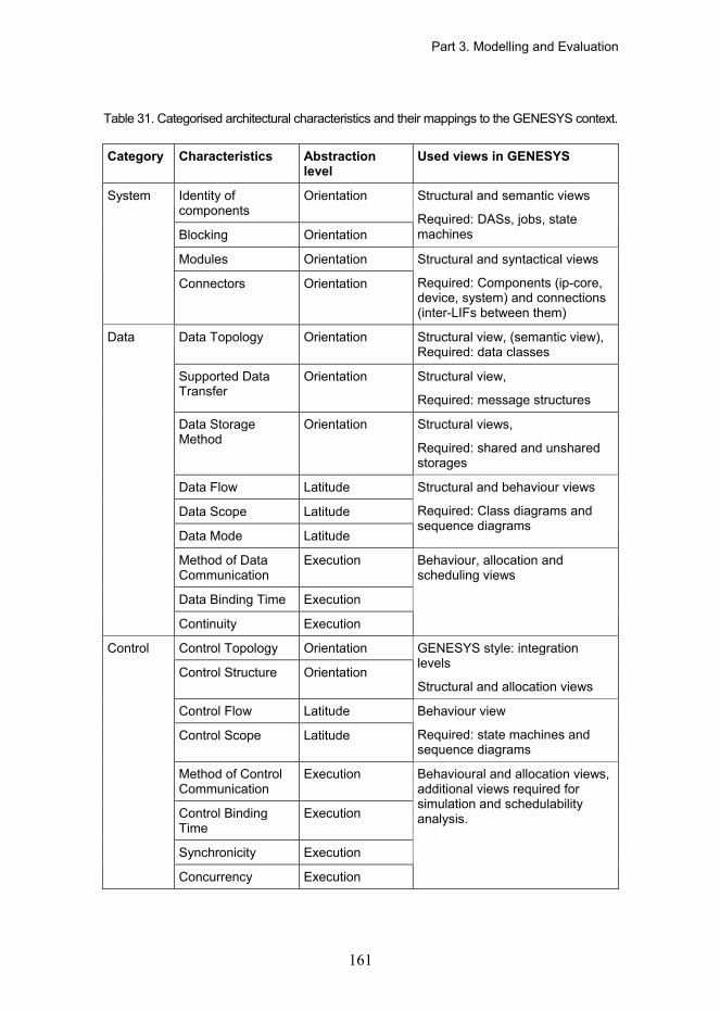
Part 3. Modelling and Evaluation
161
Table 31. Categorised architectural characteristics and their mappings to the GENESYS context.
Category Characteristics Abstraction level
Used views in GENESYS
Identity of components
Orientation
Blocking Orientation
Structural and semantic views
Required: DASs, jobs, state machines
Modules Orientation
System
Connectors Orientation
Structural and syntactical views
Required: Components (ip-core, device, system) and connections (inter-LIFs between them)
Data Topology Orientation Structural view, (semantic view), Required: data classes
Supported Data Transfer
Orientation Structural view,
Required: message structures
Data Storage Method
Orientation Structural views,
Required: shared and unshared storages
Data Flow Latitude
Data Scope Latitude
Data Mode Latitude
Structural and behaviour views
Required: Class diagrams and sequence diagrams
Method of Data Communication
Execution
Data Binding Time Execution
Data
Continuity Execution
Behaviour, allocation and scheduling views
Control Topology Orientation
Control Structure Orientation
GENESYS style: integration levels
Structural and allocation views
Control Flow Latitude
Control Scope Latitude
Behaviour view
Required: state machines and sequence diagrams
Method of Control Communication
Execution
Control Binding Time
Execution
Synchronicity Execution
Control
Concurrency Execution
Behavioural and allocation views, additional views required for simulation and schedulability analysis.
Part 3. Modelling and Evaluation
162
Steps of model-based evaluation
The model-based composability evaluation has the following steps:
• The evaluation criteria related to composability (i.e. integrability and interoperability) defined in the system specification phase are compared to the cross-domain architectural style. In a conflicting case, the style has the higher priority and the system criteria are refined so that they match with the principles of the cross-domain architecture style.
• The architectural models of the structure, semantic, behaviour and allocation views are checked against the principles of the cross-domain architecture style and the reference architecture template. Modules, connectors and supported data transfers used in models are compared to the principles defined in the cross-domain style about components, services, interfaces and messaging. The use of earlier developed application and platform services are checked against the service descriptions of the application service repository and platform service repository. The allocation and configuration views/models are checked against the rules defined for the corresponding integration levels (chip, device and system levels). After this step, the orientation level integrability and interoperability evaluation is passed.
• Next, the latitude level evaluation is made by checking the scope, mode and flow of control and data. The usage profile defined in the requirements specification phase is used for going through the scenarios based on the sequence and state diagrams of the architecture. Evaluation can be performed manually or semi-automatically. In case, the reference architecture template provides composition and binding rules, this step could be automated.
• Lastly, the syntactic evaluation is conducted. This step has to be automatic by using the properties of modern verification and simulation tools.
Recent research focuses on model-based structural and behavioural mismatch analyses and adaptation [Tsantalis 2006, Mili 2000, Canal 2008]. Structural mismatches can be identified by using a structure mapping engine [Falkenhainer 1990]. Behavioural mismatches can be removed by with or without reordering and adaptation supported by the Adaptor tool [Canal 2008].
Part 3. Modelling and Evaluation
163
3.8.9.2 Component Based Evaluation
System architecture defines the relationships that a component has with other components. Each relationship together with the interface description defines a contract between a component that provides certain functionality and the components that require that functionality. Thus, interfaces determine how a component can be used and interconnected with other components and the interface description helps integrators to decide what integration strategy to use.
Interfaces can be controlled by the following strategies:
• Use of de facto and industry-defined standards (preferably open standards).
• Specifying as many assumptions about a component�s interface as is feasible.
• Adapting the component to the use of integration elements.
Steps of component based evaluation
Next, each of these strategies are introduced and mapped to the context of the methodology framework. Thus, the component-based composability evaluation has three main steps:
1. Stability of interfaces
A number of the existing standards define how to access particular functional components. These standards take the form of an Application Programmer Interface (API) that defines how to link to a local procedure call, or they take the form of a protocol that defines how to access a service over a network. By using an industry-accepted standard, component developers provide the integrators with a much greater capability to mix and match components. However, accepted standards exist only in domains that are relatively mature.
The de facto standard is the specification of a linking interface (LIF). LIFs are the interfaces for the integration of components at a given integration level. Thus, the LIFs used/defined in the system architecture shall be checked against 1) the LIFs defined in the platform module library and 2) the new LIFs against the LIF specification defined in the cross-domain architectural style.
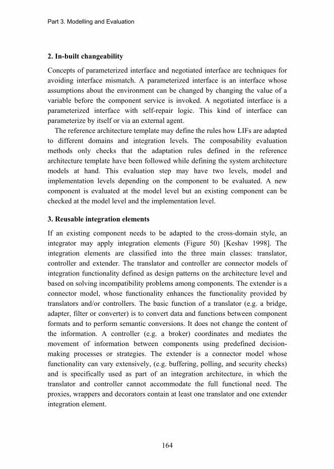
Part 3. Modelling and Evaluation
164
2. In-built changeability
Concepts of parameterized interface and negotiated interface are techniques for avoiding interface mismatch. A parameterized interface is an interface whose assumptions about the environment can be changed by changing the value of a variable before the component service is invoked. A negotiated interface is a parameterized interface with self-repair logic. This kind of interface can parameterize by itself or via an external agent.
The reference architecture template may define the rules how LIFs are adapted to different domains and integration levels. The composability evaluation methods only checks that the adaptation rules defined in the reference architecture template have been followed while defining the system architecture models at hand. This evaluation step may have two levels, model and implementation levels depending on the component to be evaluated. A new component is evaluated at the model level but an existing component can be checked at the model level and the implementation level.
3. Reusable integration elements
If an existing component needs to be adapted to the cross-domain style, an integrator may apply integration elements (Figure 50) [Keshav 1998]. The integration elements are classified into the three main classes: translator, controller and extender. The translator and controller are connector models of integration functionality defined as design patterns on the architecture level and based on solving incompatibility problems among components. The extender is a connector model, whose functionality enhances the functionality provided by translators and/or controllers. The basic function of a translator (e.g. a bridge, adapter, filter or converter) is to convert data and functions between component formats and to perform semantic conversions. It does not change the content of the information. A controller (e.g. a broker) coordinates and mediates the movement of information between components using predefined decision-making processes or strategies. The extender is a connector model whose functionality can vary extensively, (e.g. buffering, polling, and security checks) and is specifically used as part of an integration architecture, in which the translator and controller cannot accommodate the full functional need. The proxies, wrappers and decorators contain at least one translator and one extender integration element.
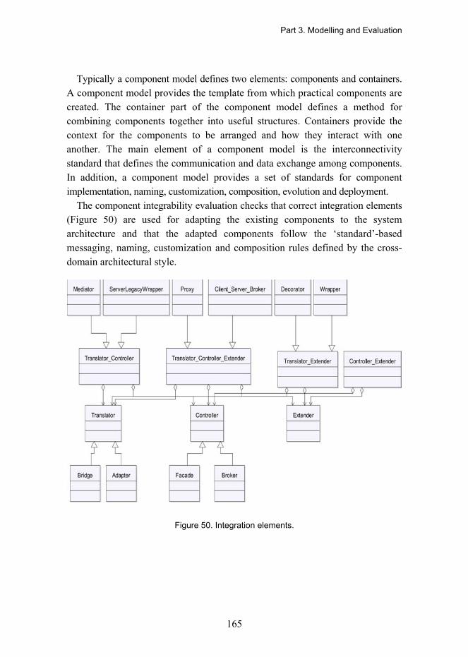
Part 3. Modelling and Evaluation
165
Typically a component model defines two elements: components and containers. A component model provides the template from which practical components are created. The container part of the component model defines a method for combining components together into useful structures. Containers provide the context for the components to be arranged and how they interact with one another. The main element of a component model is the interconnectivity standard that defines the communication and data exchange among components. In addition, a component model provides a set of standards for component implementation, naming, customization, composition, evolution and deployment.
The component integrability evaluation checks that correct integration elements (Figure 50) are used for adapting the existing components to the system architecture and that the adapted components follow the �standard�-based messaging, naming, customization and composition rules defined by the cross-domain architectural style.
Figure 50. Integration elements.

Part 3. Modelling and Evaluation
166
Tool support
If the component model defined by the cross-domain architectural style is described as a meta component model and supported by the modelling environment, the steps of the component based composability evaluation could be semi-automatic. An analyzer is needed for making the decision that appropriate integration elements are applied. Recent architectural knowledge management tools already support this step, e.g. Stylebase for Eclipse, PAMKE and WOP.
3.8.10 Evolvability Evaluation
Evolvability is a concept related to several quality attributes, e.g. flexibility, adaptability, extensibility, maintainability, and modifiability. Therefore, many evaluation methods cover one or more quality attributes of evolvability. Most of these methods are scenario-based, and thus the first step in evolvability evaluation is to define what to evaluate and why.
The selection of the evaluation method is based upon the required quality properties of the system and the supporting evaluation methods and tools. However, the importance levels of the quality properties define the order that the quality evaluation follows. The importance levels are defined by categorizing the QA requirements into three or four classes which represent how critical the QA requirements are for the success of the system architecture and products/systems based on it. An example of influence factors is introduced in Table 32. At least one of the influence factors of the selected importance level has to be true, when the evaluation order is selected. The idea is to first concentrate on the part of the system architecture that has the greatest influence on quality (e.g. size, criticality, complexity), and when that part is proved to be correct, the evaluation focuses on the other parts that have lower impact on quality.

Part 3. Modelling and Evaluation
167
Table 32. Prioritizing QAs for the evaluation order.
Importance level Sphere of interest Dependencies Impact on implementation
1 similar core services and optional services
related to many other services and QAs, trade-offs making necessary
special resources required, time-consuming, high complexity
2 specific optional /application services
related to other QA(s) special resources required, moderate complexity
3 application services no relation to other QAs
moderate/low complexity
3.8.10.1 Adaptability Evaluation
Adaptability is a quality attribute that has two different meanings: 1) a qualitative property of a system�s maintainability and 2) an ability of components/services of a system to adapt their functionality, even at runtime, to behavioural and structural changes that occur either internally or externally in their operating environment and the requirements of stakeholders� objectives [Tarvainen 2008]. Here we focus on the latter one, i.e. how to evaluate from architectural descriptions that the system to be developed has an ability to adapt its functionality in a changing environment.
The Adaptability Evaluation Method (AEM) [Tarvainen 2008] that is an integral part of QADA® (Quality driven Architecture Design and quality Analysis) methodology supports adaptability evaluation from software architecture models. AEM has three phases, each of them including several steps.
1. Adaptability requirements specification
The first phase includes the following activities:
• Identifying stakeholders and their concerns. In this phase, stakeholders are defined as actors and their adaptability requirements are analyzed and modelled in the strategic dependency model that describes dependencies between goals, soft goals (goals that can not be defined precisely), tasks and resources. The dependency model helps in negotiation and prioritization of the importance of goals.

Part 3. Modelling and Evaluation
168
• Mapping the adaptability requirements to functional blocks, i.e. sub-systems, domains, components and services. One adaptability requirement may be mapped to several functional blocks. Additionally, the adaptability requirements themselves may result in certain functionality.
• Comparison of architectural styles and selection of the optimal one. Comparison is based on the defined adaptability requirements. Patterns that support adaptability are recommended.
• Adaptability evaluation criteria are defined on tree levels: common criteria for all products (i.e. core services), 2) common criteria for domain specific services, and 3) product specific criteria.
2. Modelling adaptability
In this phase, the adaptability requirements are mapped to different architectural views; structure, behaviour and deployment. As defined in the methodology framework, structure and behaviour are described in phase 2 and 3. Deployment is defined in phase 4 when application and platform models are combined. Thus, the adaptability requirements mapping has to be considered in all three architecture design phases.
3. Adaptability evaluation
Qualitative adaptability evaluation means tracking if adaptability requirements are met. The use of qualitative adaptability evaluation requires traceability support from the modelling environment. When this kind of support is available, this evaluation phase is automatic; the designer maps the adaptability requirements to architectural elements in the design phase, and in the evaluation the modelling environment informs only if some of the adaptability requirements are not handled.
Quantitative adaptability evaluation assists the user in selecting the optimal architecture among the candidate architectures. Stakeholders� adaptability goals drive the evaluation as follows:
• The adaptability scenario profile is defined for each architecture candidate based on the defined adaptability goals. The adaptability scenarios defined in the profile are descriptions of a system�s behaviour driven by potential changes related to adaptability.
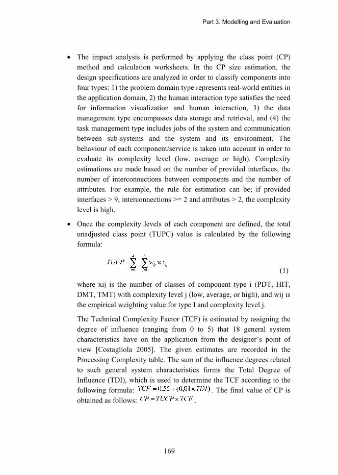
Part 3. Modelling and Evaluation
169
• The impact analysis is performed by applying the class point (CP) method and calculation worksheets. In the CP size estimation, the design specifications are analyzed in order to classify components into four types: 1) the problem domain type represents real-world entities in the application domain, 2) the human interaction type satisfies the need for information visualization and human interaction, 3) the data management type encompasses data storage and retrieval, and (4) the task management type includes jobs of the system and communication between sub-systems and the system and its environment. The behaviour of each component/service is taken into account in order to evaluate its complexity level (low, average or high). Complexity estimations are made based on the number of provided interfaces, the number of interconnections between components and the number of attributes. For example, the rule for estimation can be; if provided interfaces > 9, interconnections >= 2 and attributes > 2, the complexity level is high.
• Once the complexity levels of each component are defined, the total unadjusted class point (TUPC) value is calculated by the following formula:
(1)
where xij is the number of classes of component type i (PDT, HIT, DMT, TMT) with complexity level j (low, average, or high), and wij is the empirical weighting value for type I and complexity level j.
The Technical Complexity Factor (TCF) is estimated by assigning the degree of influence (ranging from 0 to 5) that 18 general system characteristics have on the application from the designer�s point of view [Costagliola 2005]. The given estimates are recorded in the Processing Complexity table. The sum of the influence degrees related to such general system characteristics forms the Total Degree of Influence (TDI), which is used to determine the TCF according to the following formula: . The final value of CP is obtained as follows: .
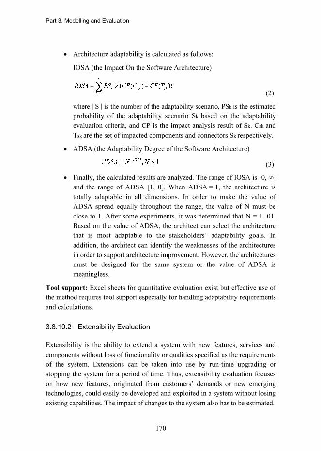
Part 3. Modelling and Evaluation
170
• Architecture adaptability is calculated as follows:
IOSA (the Impact On the Software Architecture)
(2)
where | S | is the number of the adaptability scenario, PSk is the estimated probability of the adaptability scenario Sk based on the adaptability evaluation criteria, and CP is the impact analysis result of Sk. Csk and Tsk are the set of impacted components and connectors Sk respectively.
• ADSA (the Adaptability Degree of the Software Architecture)
(3)
• Finally, the calculated results are analyzed. The range of IOSA is [0, ∞] and the range of ADSA [1, 0]. When ADSA = 1, the architecture is totally adaptable in all dimensions. In order to make the value of ADSA spread equally throughout the range, the value of N must be close to 1. After some experiments, it was determined that N = 1, 01. Based on the value of ADSA, the architect can select the architecture that is most adaptable to the stakeholders� adaptability goals. In addition, the architect can identify the weaknesses of the architectures in order to support architecture improvement. However, the architectures must be designed for the same system or the value of ADSA is meaningless.
Tool support: Excel sheets for quantitative evaluation exist but effective use of the method requires tool support especially for handling adaptability requirements and calculations.
3.8.10.2 Extensibility Evaluation
Extensibility is the ability to extend a system with new features, services and components without loss of functionality or qualities specified as the requirements of the system. Extensions can be taken into use by run-time upgrading or stopping the system for a period of time. Thus, extensibility evaluation focuses on how new features, originated from customers� demands or new emerging technologies, could easily be developed and exploited in a system without losing existing capabilities. The impact of changes to the system also has to be estimated.

Part 3. Modelling and Evaluation
171
The IEE method is intended for evaluating integrability and extensibility of software (family) architectures [Henttonen 2007]. The method is scenario-based and aligned with the principles of QADA. The phases of IEE can be mapped to the following phases of the modelling process; requirements specification, architecture modelling and quality evaluation. The extensibility evaluation part of the method could be adopted for the methodology framework as follows:
1. Defining quality goals and quality criteria
The phase includes four activities: impact analysis, quality analysis, variability analysis and hierarchical domain analysis. Domain experts are responsible for impact analysis and quality analysis. In the impact analysis, the domain experts identify and elicit the interests of the business stakeholders and technical stakeholders, define the standards, regulations and practices to be followed in the domain. This activity means adaptation of the methodology framework into practice and results in a list of the stakeholders and their quality goals.
Application and platform architects identify and define core and domain specific functional and quality properties of a system (i.e. variability analysis), and categorize capabilities into a service taxonomy taking into account the defined functional capabilities, quality goals, domain specificity and commonality of the capabilities (i.e. hierarchical domain analysis). The phase results in a list of prioritized quality criteria against which the architecture is evaluated. Instructions how to define quality goals and quality criteria, and how to represent the required and provided quality properties in architectural models are given in [Niemelä 2007].
2. Defining and modelling change scenarios for extensibility evaluation
Phase 2 includes one combined activity: scenario modelling. The purpose of this phase is to define and model a representative set of change scenarios and, if necessary, enhance the existing architectural description with information relevant to the extensibility evaluation. The scenarios represent possible future needs with regard to extension of products based on the architecture. The scenario modelling consists of the following tasks: 1) defining scenarios for extensibility, 2) selecting appropriate views and patterns for describing architecture, and 3) defining assumptions, architectural constraints and a design rationale for each view. The phase results in the description of system architecture at the point where all figurative change scenarios have been
Part 3. Modelling and Evaluation
172
realized. The description includes a complete set of views and selected styles and patterns. The cross-domain architecture style and architectural views have already been defined. Selection of patterns depends on the application under development.
3. Extensibility evaluation from architectural models
In the third phase, quality analysts evaluate the extensibility of the architecture and compare the evaluation results to the defined quality criteria. In quality evaluation, extensibility analysis is used to identify in which part the architecture extension points are required and how effectively extensibility patterns are used in the architecture. Comparative analysis is applied to compare the evaluation results to the quality criteria, identifying conflicts and the making of trade-offs, and finally evaluation results are reported as proposed improvements and as identified unsolved problems, which are returned to the architects for the next iteration phase.
The quality evaluation is done iteratively and incrementally. First, the quality criteria, which have high importance and affect many parts of the architecture, are evaluated. If these qualities do not meet the requirement, architecture refinement is needed and after refinement the quality criteria of high importance are re-evaluated. Secondly, quality criteria of high importance but small impact are evaluated. Third, quality criteria of medium importance for any part of the architecture are taken under evaluation. Last, quality criteria of low importance are checked. The approach allows the evaluator to focus first on the most important qualities and thereafter to make trade-offs among the less important quality criteria.
3.8.10.3 Maintainability, Flexibility and Modifiability Evaluation
Maintainability, flexibility and modifiability address the ability to improve and change a system easily. Maintainability is the ease with which a system/component/service can be modified. Modification may mean removal, update, addition or moving a component/service to a different computing node. Flexibility is the ease with which a system or component can be modified for use in applications or an environment other than those for which it was specifically designed. Modifiability for its part measures how quickly and cost-effectively the changes can be made.

Part 3. Modelling and Evaluation
173
Architecture level modifiability analysis (ALMA) was selected from a set of different methods because of its obvious superiority over other similar kinds of methods; it has a clearly defined process, it has been applied to industrial cases and the method supports multi-goal evaluation [Bengtsson 2004].
The separation between the tasks of the following steps is not strict and it is often necessary to iterate over various steps.
1. Select the evaluation goal
• Maintenance cost prediction by estimating the effort required to modify the system to accommodate future changes.
• Risk assessment by identifying the types of changes for which the architecture is inflexible.
• Architecture selection by comparing candidates and selecting the optimal one.
2. Describe the relevant parts of the architecture
Modifiability evaluation requires architectural information that allows the analyst to evaluate the scenarios. The following information is needed: decomposition of the system into components, relationships between components and relationships between the system and its environment. All relationships are not known at the architecture level because they are defined in detailed design or implementation. These relationships may cause unforeseen triple effects when modifications are made to a component. Because it is not always possible to determine the full impact of a scenario, this affects the overall accuracy of evaluation, which is based on the sufficiency of available information. If the information proves to be insufficient to determine the effect of the scenarios found, there are two options. First, it is not possible to determine the effect of the scenario precisely. Alternatively, the architect that assists in scenario evaluation may fill in the missing information.
3. Define the set of relevant change scenarios
There are a couple of issues in the elicitation of change scenarios: the number of possible changes and selection criterion. The number of possible changes to a system is almost infinite. In order to make scenario-based evaluation feasible, a combination of two techniques is used: equivalence classes and classification of change categories.

Part 3. Modelling and Evaluation
174
Partitioning the space of scenarios into equivalence classes enables one to treat one scenario as a representative of a class of scenarios, thus limiting the number that have to be considered. However, not all equivalence classes are just as relevant for each analysis. Deciding on important change scenarios requires a selection criterion. Classification of change categories is used to focus on the scenarios that satisfy this selection criterion.
There are two approaches for selecting a set of scenarios: top-down and bottom-up. In a top-down approach some predefined classification of change categories guides the search for change scenarios. This classification may derive from the domain of interest, knowledge of potentially complex scenarios, or some other external knowledge source. In interviews with stakeholders, the analyst uses this classification scheme to stimulate the interviewee to bring forward relevant scenarios. This approach is top-down, because the analyst starts with high-level classes of changes and concludes with concrete change scenarios. When using a bottom-up approach, there is no predefined classification scheme but it is left to the stakeholders being interviewed to come up with a relevant set of scenarios. The analyst then categorizes the scenarios and stakeholders review this categorization. In practice, the approaches are iterated such that the elicited change scenarios are used to build up or refine the classification scheme. This (refined) scheme is next used to guide the search for additional scenarios. In addition to the selection criterion, elicitation also needs a stopping criterion to decide when a representative set of scenarios have been collected. In ALMA, the number of change scenarios is sufficient when: (1) all change categories are explicitly considered and (2) new change scenarios do not affect the classification structure.
The second issue is that of deciding on the selection criterion. The selection criterion for scenarios is closely tied to the goal of evaluation. If the goal is to estimate maintenance effort, the focus is on scenarios that correspond to changes that have a high probability of occurring during the operational life of the system. If the goal is to assess risks, the analyst selects scenarios that expose those risks. If the goal is to compare different architectures, the analyst concentrates on scenarios that highlight differences between those architectures. Table 33 introduces the different means of defining change scenarios and when to use them (based on Architecture Trade-off Analysis Method, ATAM).

Part 3. Modelling and Evaluation
175
Table 33. Means for defining change scenarios.
Means Sub-type Used for
Direct scenario eliciting information about the architecture
representing changes to the system
growth scenario representing anticipated future changes; predicting maintenance effort
Indirect scenario
exploratory scenario stressing the system, exposing the limits of the current design
Utility tree top-down decomposition of relevant quality attributes in the assessment (modifiability)
Facilitated brainstorming
a bottom-up mechanism
4. Determine the effect of the set of scenarios
Scenario evaluation concerns two steps: analysis of the impact of the scenarios and expressing this impact. Architecture-level impact analysis is used to identify the architectural elements affected by a change scenario. This includes the components that are affected directly, but also the indirect effects of changes on other parts of the architecture. The effect of the scenario is expressed using some measurement scale, depending on the goal of the modifiability analysis.
Together with the architects and designers the analyst determines the impact of the change scenarios and expresses the results in a way suitable to the goal of evaluation. This is the architecture level impact analysis that consists of the following steps:
• Identifying the affected components, i.e. the components to be modified.
• Determining the effect on the components, i.e. the functions of the components to be changed and how changes propagate over system boundaries (interfaces to environment).
• Determining ripple effects. The occurrence of ripple effects is recursive; each ripple may have additional ripple effects. Because not all information is available at the architecture level, the analyst has to make assumptions about the occurrence of ripple effects. The optimistic assumption is that there is no ripple effect. The pessimistic
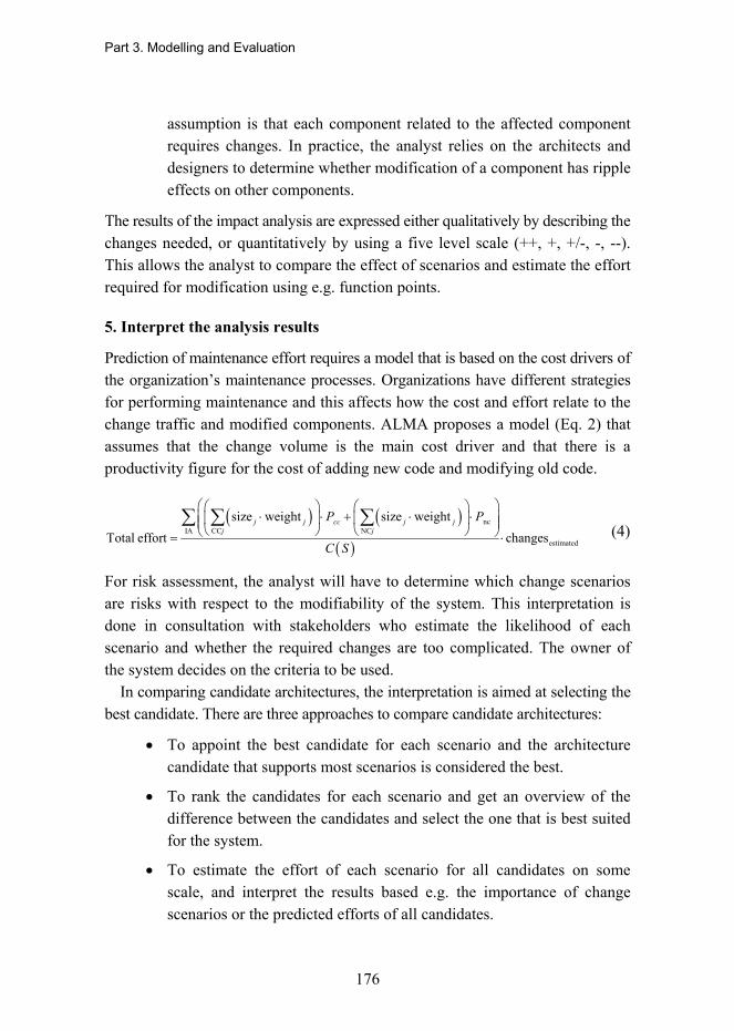
Part 3. Modelling and Evaluation
176
assumption is that each component related to the affected component requires changes. In practice, the analyst relies on the architects and designers to determine whether modification of a component has ripple effects on other components.
The results of the impact analysis are expressed either qualitatively by describing the changes needed, or quantitatively by using a five level scale (++, +, +/-, -, --). This allows the analyst to compare the effect of scenarios and estimate the effort required for modification using e.g. function points.
5. Interpret the analysis results
Prediction of maintenance effort requires a model that is based on the cost drivers of the organization�s maintenance processes. Organizations have different strategies for performing maintenance and this affects how the cost and effort relate to the change traffic and modified components. ALMA proposes a model (Eq. 2) that assumes that the change volume is the main cost driver and that there is a productivity figure for the cost of adding new code and modifying old code.
( ) ( )( )
ncIA CC NC
estimated
size weight size weightTotal effort changes
j j cc j jj j
Ρ Ρ
C S
⎛ ⎞⎛ ⎞ ⎛ ⎞⋅ ⋅ + ⋅ ⋅⎜ ⎟⎜ ⎟ ⎜ ⎟⎜ ⎟⎝ ⎠ ⎝ ⎠⎝ ⎠= ⋅
∑ ∑ ∑ (4)
For risk assessment, the analyst will have to determine which change scenarios are risks with respect to the modifiability of the system. This interpretation is done in consultation with stakeholders who estimate the likelihood of each scenario and whether the required changes are too complicated. The owner of the system decides on the criteria to be used.
In comparing candidate architectures, the interpretation is aimed at selecting the best candidate. There are three approaches to compare candidate architectures:
• To appoint the best candidate for each scenario and the architecture candidate that supports most scenarios is considered the best.
• To rank the candidates for each scenario and get an overview of the difference between the candidates and select the one that is best suited for the system.
• To estimate the effort of each scenario for all candidates on some scale, and interpret the results based e.g. the importance of change scenarios or the predicted efforts of all candidates.

Part 3. Modelling and Evaluation
177
3.8.10.4 Trade-off Analysis
The Architecture Trade-off Analysis Method®1(ATAM) is a method for evaluating software architectures relative to quality attribute goals. ATAM consists of the following phases and steps:
Phase 1: Presentation
• Method. The analyst describes ATAM to the assembled participants, tries to set their expectations, and answers questions they may have.
• Business drivers. The project manager or system customer describes what business goals motivate the development effort and what the primary architectural drivers are.
• Architecture. The architect describes the architecture focusing on how it addresses the business drivers.
Phase 2: Investigation and analysis
• Architectural options are identified.
• Quality attribute utility tree. Quality attributes that comprise system �utility� are elicited, specified by scenarios and annotated with stimuli and responses, and finally prioritized.
• Analysis of the architectural options. Those architectural options that address the scenarios of high priority are analysed by identifying risks, non-risks, sensitivity points and trade-offs points.
Phase 3: Testing
• Brainstorm and prioritized scenarios. A larger set of scenarios is elicited from the group of stakeholders and prioritized via a voting process by all the stakeholders.
• Analysis of the architectural options. The defined larger set of scenarios is used as test cases for analysing and ranking the architectural options.
1 ®ATAM is registered in the U. S. Patent and Trademark Office by Carnegie Mellon Software Engineering Institute.
Part 3. Modelling and Evaluation
178
Phase 4: Reporting
• The evaluation team presents the collected results (options, scenarios, attribute-specific questions, the utility tree, risks, non-risks, sensitivity points, tradeoffs) to the assembled stakeholders.
With regard to the previously presented methods, the Software Engineering Institute (SEI) has applied ATAM to the evaluation of industrial system architectures during the last ten years and distilled the risks into themes that summarize and consolidate the collection of risks found during evaluations. The risk themes are based on 18 architecture evaluations [Bass 2006]. As a result, the four most prevalent risk theme categories were identified: performance, requirements, unrecognized needs and organizational awareness. 14 of the evaluated systems were different kinds of embedded systems. In more than 10 cases performance, reliability/availability and interoperability were considered as business goals in a similar way as functionality. Performance in particular was considered as an important business goal. Naturally, the cost of development, deployment, operation and maintenance were also ranked high. Similarity among the risk theme categories of high importance and the prioritized quality attributes of the methodology framework is evident.
In four domains, more than one evaluation was made. When comparing the evaluation results, it was seen that that there is no similarity among the risk themes of the evaluations in any of the four domains. One explanation may be that the organizational context plays a part in the generation of risk themes.
Risk themes were categorized into three types:
• risks of commission resulting from problematic architectural decisions, • risks of omission resulting from not performing a certain activity/activities. • neither commission nor omission; ambiguous risks.
Three risks of omission were identified: security, requirements and unrecognized needs. The last two risk themes are not the result of architectural decisions but rather the results of having a high level of uncertainty in requirements and/or stakeholders� needs. The security risk themes were not all of risks of omission. In fact, security requirements are hard to meet, and architectural teams ignored some important aspects of meeting them.

Part 3. Modelling and Evaluation
179
3.8.11 Summary of Quality Evaluation
To summarize the quality evaluation methods selected for the methodology framework, the most important findings related to the important quality attributes of embedded systems are:
• Performance. Two performance evaluation methods were introduced. The software performance evaluation method is based on LQN models contrary to the application-platform performance evaluation method that requires workload models and transaction-level capacity models. Both methods are applicable within UML-MARTE models and have, at least, partial tool support.
• Power/energy efficiency. One evaluation method was introduced. The method requires a multiprocessor simulation platform and power models as input. Tooling is still on the research prototype level.
• Reliability and availability. Three evaluation methods were introduced. Methods require input sequence diagrams, state diagrams, usage profiles and probabilities of state transitions/transactions. Two of the methods are supported by appropriate tools.
• Safety. Two safety evaluation methods were introduced. The Hip-HOPS method was recommended for assessing GENESYS platforms and the NuSMV method for safety evaluation in model-driven development. Use of Hip-HOPS requires adaptation between MARTE and ATTEST-ADL2. NuSMV requires mapping between UML MARTE and evaluation tools.
• Composability. Two approaches were proposed for the composability evaluation; model-based and component-based evaluation. The model-based approach is usable in top-down design. Conformance of existing artefacts, i.e. components and services, against the GENESYS architectural style and template is to be checked by using the component-based evaluation method when the bottom-up approach is used.
• Evolvability. Three methods were proposed for evolvability evaluation. All of these methods are scenario-based and partially qualitative, although there are also quantitative measures. ADM measures the adaptability degree of architecture and compares it to the adaptability
Part 3. Modelling and Evaluation
180
criteria. Extensibility evaluation shows how well the architecture is supported by extension points for new features, services and components. ALMA measures how easily a system can be improved and changed. Cost-effectiveness can also be measured. A common shortcoming for all of these methods is that they are laborious without tool support and their application requires specific skills.
• Trade-offs. One method was introduced for trade-off analysis, ATAM, although the above mentioned evolvability evaluation methods also support trade-offs making, mostly adopted from ATAM. The strength of ATAM is its applications to embedded systems in industrial settings. The use of the method is fully dependent on the skills of the method users and without any tool support.

181
Part 4. Conclusions and Future Work 4.1 Overview
Although a large amount of commercial and open source tools for modelling and quality evaluation exists, an integrated development environment is required in order to provide smooth transformation from one design phase to another and keep the models in a consistent state. Therefore, a strong development effort should be made for developing this kind of integrated development environment for embedded systems engineering. In this section, such design environment is outlined. Thereafter, the methodology framework is evaluated by comparing its support to the principles defined in Part 1.
4.2 Integrated Development Environment
4.2.1 Extra Requirements
Besides the eighth principles of the methodology framework introduced in Part I there are additional requirements that are implicit because they are invisible or natural from the user point of view.
4.2.1.1 Support for Multiple Modelling Languages
All the requirements combined in the eighth principle rely on the support of model language handling. Without this feature, code generation, model transformation, and model-based hardware software integration cannot exist. The environment should support the application of multiple (and most probably domain-specific) modelling languages simultaneously.

Part 4. Conclusions and Future Work
182
Besides having multi-language modelling support, the inter-language links should also be possible. The overall design artefact traceability is built on that while defining inter-model references.
Current solutions like Eclipse Modeling Framework (EMF) [EMF 2008], MetaData Repository (MDR) [MDR 2008] and Visual and Precise Metamodelling (VPM) [Varró 2004] all support the definition of multiple modelling languages and the manipulation of multiple model instances simultaneously.
4.2.1.2 Collaborative Development Support
Collaborative or team development has a long tradition in IT systems development, and simultaneously with the growing complexity and size of systems under design it has gained even more importance. The support for it should be an integral part of the development environment. It should be noted that although most of the current solutions offer such functionality for source code sharing and versioning, the same should also be present for models and other design artefacts.
4.2.1.3 Open, Extensible Design Environment
Given the high diversity in the target application domain, the design environment should be extensible in order to be customizable for new implementation targets, new modelling aspects, and new analysis tools. The extension interfaces should be public in order to allow tool vendors to contribute to the environment resulting in a multi-vendor tool chain configuration assembled by the tool components most suitable for the user (and for the actual development project).
4.2.2 Integrated Design Environment
This Section will introduce the proposed architecture for the integrated design environment based on the requirements discussed earlier. The high level architecture of the tool environment is illustrated by Figure 51.
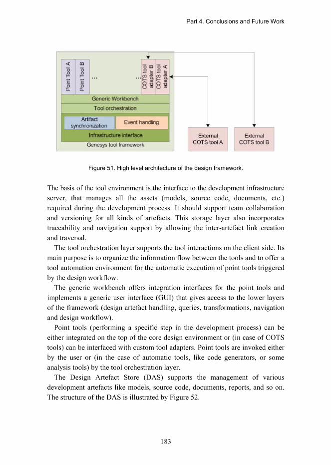
Part 4. Conclusions and Future Work
183
Figure 51. High level architecture of the design framework.
The basis of the tool environment is the interface to the development infrastructure server, that manages all the assets (models, source code, documents, etc.) required during the development process. It should support team collaboration and versioning for all kinds of artefacts. This storage layer also incorporates traceability and navigation support by allowing the inter-artefact link creation and traversal.
The tool orchestration layer supports the tool interactions on the client side. Its main purpose is to organize the information flow between the tools and to offer a tool automation environment for the automatic execution of point tools triggered by the design workflow.
The generic workbench offers integration interfaces for the point tools and implements a generic user interface (GUI) that gives access to the lower layers of the framework (design artefact handling, queries, transformations, navigation and design workflow).
Point tools (performing a specific step in the development process) can be either integrated on the top of the core design environment or (in case of COTS tools) can be interfaced with custom tool adapters. Point tools are invoked either by the user or (in the case of automatic tools, like code generators, or some analysis tools) by the tool orchestration layer.
The Design Artefact Store (DAS) supports the management of various development artefacts like models, source code, documents, reports, and so on. The structure of the DAS is illustrated by Figure 52.

Part 4. Conclusions and Future Work
184
The DAS is a server component that stores the design artefacts in a central (versioning) repository. It also contains an artefact catalogue (project tree for all development projects) and user rights management in order to support the access control rule definition on the various design artefacts. The query engine (file and model element level query support) supports the definition of custom queries/views on the repository or on different models. The navigation and traceability support module implements a uniform inter-element trace definition, maintenance, and navigation framework that allows the tracing of concepts throughout design steps. The model transformation module executes automatic transformations on the various elements in order to synchronize various models or to derive analysis models from engineering ones.
The communication and event layer serves as a interface for the developer PCs (clients) that run the Integrated Development Environment. The client-server architecture allows for a real-time team collaboration both in models and textual documents and the immediate synchronization of models between developers on model changes.
Figure 52. Architecture of the Design Artefact Store.

Part 4. Conclusions and Future Work
185
4.2.2.1 Versioning Artefact Storage
This component�s main responsibility is the storage of design artefacts. Besides this, it also stores project-related meta data such as the workflow of the development process, the current status of the tasks, and the list and rights of project members (analysts, system designers, architects, developers, and so on).
In contrast with the current versioning systems solutions (like CVS, Subversion, Microsoft Team Foundation Server, and Rational ClearCase) that rely on file-based versioning and text level file comparison, the proposed solution relies on a finer grained level in the case of models. Model changes are handled at the model element level, and the changes are organized into user transactions. After a transaction is executed, the model changes are directly propagated to all clients and that results in a live synchronization. Model versions are snapshots that reflect the state of the model at a given time point. The various versions are comparable also on model element level. The files are handled in the conventional way, using existing technologies.
The versioning system also includes the creation of branches that can be used to evaluate alternative design options. After creating multiple branches, the various options can be implemented and a comparative analysis can be performed on them.
4.2.2.2 Artefact Catalogue and Access Rights Management
This module is responsible for the maintenance of a catalogue of the design artefacts in the development project and the management of access rights on these elements.
The catalogue contains basic information on the artefacts (name, creation date, modification date, size, etc.), access control information, and meta information about the artefact and the tools that handle it.
The user rights management relies on an internal or external (standards compliant) user database, and is based on the RBAC (role-based access control) paradigm. User rights on artefacts can be set at element, category, or folder (sub-catalogue) level.

Part 4. Conclusions and Future Work
186
4.2.2.3 Query Services
The Query services module is responsible for the execution of queries on the design artefacts. In a textual content, it serves as an advanced search engine, while on structured content (models) it serves as model-element level query engine.
Besides the user-directed query execution, model queries are the basis of all code generation and model transformations. Given the possible high number of modelling and analysis aspects, and the large size of models, an effective query method should be used.
The queries can be executed either in batch or in live mode. Live queries reflect on model changes and are mainly used to implement event-triggered transformations or model synchronization.
Batch queries and transformations are supported by several solutions (like ATL [ATL 2008] and VIATRA2 [VIATRA 2008]) but there is only a limited set of existing tools for the live mode.
4.2.2.4 Navigation and Traceability
Traceability of requirement throughout the development process is a high priority issue in most design domains. The navigation and traceability module is responsible for the definition of trace links between artefacts (and sub elements, like model elements or text fragments) and the management of links. Trace links can be created by the user, or during the execution of automatic transformations.
4.2.2.5 Model Transformation Engine
This module relies on the services of the previous two in order to support the execution of model transformations. However, there are several existing tools and solutions for model-to-model and model-to-code transformations, like ATL, VIATRA2, etc., and these should be developed in order to include live transformation and model traceability. The central execution of transformations can result in a reduced workload on the clients, as all transformations are only executed once, and their results is propagated to the clients only when necessary.

Part 4. Conclusions and Future Work
187
4.2.2.6 Workflow Orchestration Layer
The tool orchestration layer is responsible for the execution of the development process according to the custom, pre-defined process model (defined for instance using SPEM). This includes the guidance of the user through the manual and semi-automatic steps, and the execution of automatic steps (code generation, analysis, unit tests, etc.). The status of the workflow is persisted on the server, and is distributed among the clients
4.2.2.7 Client Communication and Event Dispatching
This module has two tasks. It handles the client-server communication and central event processing.
The communication between the server and client should be platform-independent and secure. As the communication channel is extensively used during user-interactive editing, an optimized protocol offering high bandwidth and low latency.
The event dispatcher collects artefact-related events and distributes them between the clients. This is the basis of live synchronization. The clients can immediately reflect the model changes by refreshing the current view, if affected by the model changes.
4.2.3 Model Transformations
The GENESYS tool environment has to support several different model transformations in order to provide all the functionalities described in the earlier parts. In the following, a brief outline of the most important transformations will be given.
Figure 53 illustrates the key transformation paths in the development workflow. Only some important models and modelling languages are shown. Dashed lines represent manual or semi-automatic transformations, continuous lines represent automatic ones. Bi-directional arrows represent bi-directional (or synchronization-like) transformations.

Part 4. Conclusions and Future Work
188
Figure 53. Overview of transformations in the development workflow.
4.2.3.1 From requirements to PIM and PM
This transformation is traditionally manual. The main reason of treating this manual (and in most cases complex) process as a model transformation is that the traceability of requirements to model artefacts should be maintained. The role of the development environment in this case is the support of the definition of trace links, and the analysis of the models (whether all requirements have implementation in the PIM or PM).
4.2.3.2 PIM-related Transformations
Multiple PIM Representations
The main modelling notation of PIM uses UML MARTE. Although this modelling language is expressive enough to capture the concepts of a platform-independent model, several target domains have their own domain-specific language for architecture design (like AutoSAR in the automotive domain). In order to support these DSLs while keeping the standard internal MARTE model representation, DSL to MARTE transformations are needed.
Part 4. Conclusions and Future Work
189
These model transformations should be live, bi-directional and incremental, in order to be able to synchronize the models during editing. This way, the actual PIM is always present in both notations. The DSL notation is used for editing, while the MARTE model can be used for early V&V and model analysis.
Architecture and Behaviour Modelling
While MARTE (or a DSL) is used for platform-independent architecture modelling, the modelling of the internal behaviour of atomic GENESYS components is not covered by these methods. There are several languages and tools that are used traditionally in the embedded systems field to model behaviour. Matlab/Simulink, SCADE are such commercial tools, but new approaches like BIP are also important in this development step.
The main goal of the behavioural model <-> PIM transformation is the synchronization of component interfaces. While the internals of a component are modelled using a behavioural modelling language, the inter-component communication and architecture is modelled using MARTE. The consistency of the two aspects is crucial for the success of component integration.
4.2.3.3 Import from Model Libraries / Repositories
Both PIM and PM components can be stored in repositories or libraries in order to facilitate the reuse of components. The instantiation or import of these model fragments is also an important model transformation in the tool environment.
Model fragment imports usually involve some kind of model merge operations that leads to quite complex model manipulations that can efficiently handled by high level transformation methods and tools.
4.2.3.4 System Allocation / Configuration / Refinement
This development step is known as PIM-PSM mapping in the traditional MDA (Model-Driven Architecture) paradigm. The application model (PIM) is mapped to the execution platform (PM) and all necessary configurations are generated in order to produce the implementation-level platform specific model (PSM) of the system.
While this step is treated as an atomic, automatic model transformation in the traditional MDA approach, recent projects (like DECOS [DECOS 2008, Shariful 2006]) have shown that in the case of embedded systems, PIM-PSM mapping
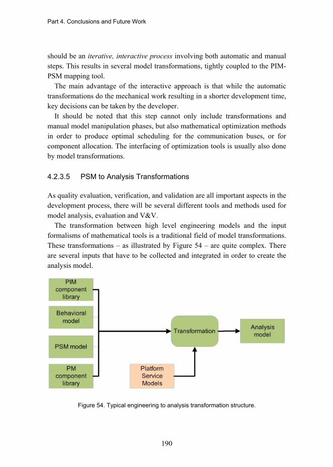
Part 4. Conclusions and Future Work
190
should be an iterative, interactive process involving both automatic and manual steps. This results in several model transformations, tightly coupled to the PIM-PSM mapping tool.
The main advantage of the interactive approach is that while the automatic transformations do the mechanical work resulting in a shorter development time, key decisions can be taken by the developer.
It should be noted that this step cannot only include transformations and manual model manipulation phases, but also mathematical optimization methods in order to produce optimal scheduling for the communication buses, or for component allocation. The interfacing of optimization tools is usually also done by model transformations.
4.2.3.5 PSM to Analysis Transformations
As quality evaluation, verification, and validation are all important aspects in the development process, there will be several different tools and methods used for model analysis, evaluation and V&V.
The transformation between high level engineering models and the input formalisms of mathematical tools is a traditional field of model transformations. These transformations � as illustrated by Figure 54 � are quite complex. There are several inputs that have to be collected and integrated in order to create the analysis model.
Figure 54. Typical engineering to analysis transformation structure.

Part 4. Conclusions and Future Work
191
The main information source is the PSM model. (It should be noted, that PIM-level analysis transformations are also common. In this case PIM is used instead of PSM). The information is complemented by the behavioural model of the application components (if the analysis tool performs detailed analysis), the respective behavioural models of the PIM and PM components that are reused from the libraries, and by the formal models of the platform services.
All these models are combined and translated to the input language of the analysis tool. It should be noted, that although this scenario is quite complex, in several cases there may be simplifications of it. There are methods that treat components as black boxes, and focus only on their interactions (timeliness and schedulability analysis, etc.). In such cases, some of the input models of the picture can be neglected.
4.2.3.6 Source and Configuration Files Generation
Source and configuration file generation is the final stage that includes model transformations (model-to-text). The goal is to generate all the necessary files for building and deploying the application on the target system.
Model-to-text transformations are supported by most model transformation frameworks and can easily be tailored to any concrete syntax needed by the target environment.
4.2.4 Available Technologies for the Tool Development
There are several promising technologies already on the market (or still emerging) that can be utilized in order to build the tool environment proposed in the last Sections. However, while these technologies are not always mature enough to have accumulated a significant amount of field experience, their features cover most of the important services of the GENESYS development infrastructure. Several open points and research items have also been identified that should be addressed in order to get a full implementation of the environment.
4.2.4.1 Available Technologies
The IBM Jazz platform [Jazz 2008] is a novel integrated collaboration enablement technology. It is still under development, but it support nearly all the features

Part 4. Conclusions and Future Work
192
required for the Infrastructure Server of the GENESYS tool chain. It contains a versioning artefact store (only at file level), collaboration utilities, requirements management and a traceability framework as well as a customizable design workflow. Its main drawback is the lack of central model management and transformation support, and the lack of tool automation support. As it has an open, extensible architecture, these missing functions can be added by integrating other tools to it.
Eclipse EMF CDO [CDO 2008] is a distributed implementation of the industry standard Eclipse Modeling Framework (EMF). It features a central model repository stored in a standard relational database that can be reached by multiple clients simultaneously. Although some important features are still missing (e.g. model versioning) it can be a solid foundation for the model artefact store. Given its open architecture, the integration of versioning and query/transformation support should be feasible.
One of the key technologies is the selection of an appropriate model transformation technique. The complexity and diversity of transformations during the development process necessitates the selection of a powerful tool. There are several proposals, like VIATRA2 [VIATRA 2008] and ATL [ATL 2008] from the Eclipse project, but none of them has all the required features (live and batch transformations, EMF integration, incremental pattern matching, etc.).
In the case of client side technologies, the selection is straightforward. The Eclipse Framework is the most widespread tool integration framework nowadays, and its importance is still growing. It contains several components that can be easily reused by the tool environment.
4.2.4.2 Research and Development Items
An important research item is the extension of the traceability support currently available. Although there are several solutions for that, up to now there has been no uniform, extensible solution. Traceability is a complex problem involving all tools, transformations, and model/file management components of the tool environment; therefore a global solution should be proposed.
The integration of distributed model storage and model transformation support also needs further investigation. There are currently several promising technologies in both areas, but no integrated solution exists. The support for integrated, automated model-to-model and model-to-text transformations is a key to the success of the model-driven development approach.

Part 4. Conclusions and Future Work
193
The enablement of model / model element level versioning and concurrent model manipulation is also a key technology in team collaboration-based development. Industrial practice shows that the current edit and merge techniques are inappropriate in most cases. There are dedicated tools that use the concept of distributed model editing and enable concurrent modifications, but no general solution is present.
As a summary, we can state that most of the important technologies are present currently, but there are several missing elements that should be created in order to achieve a complete model-driven tool chain that will be capable of handling real size development projects.
4.3 Evaluating Methodology Framework
The definition of the methodology framework is based on eight principles which were derived from the requirements identified and defined by the authors with the help of industrial partners involved in the GENESYS project. To summarize, we justify the completeness of the methodology framework by illustrating how these principles are supported by the methodology framework.
Principle 1: Embedded systems engineering process
The methodology framework provides the following support for the whole life-cycle of embedded systems engineering:
• A process model with appropriate modelling and evaluation methods that support modelling and early verification and validation from requirements specification to validated system architecture models (top-down approach).
• Each modelling and evaluation phase is supported by a set of tools which can be integrated by means of the platform of the integrated tool environment.
• Adoption of the UML-MARTE modelling language is supported by guidelines and a numerous set of examples.
• A process model defines how the existing services and components from the application service repository and the platform module library could be used (bottom-up approach) in application and platform architecture design.

Part 4. Conclusions and Future Work
194
It should be noted that the methodology framework allows for exploration, refinement and iteration. For example, the approach can be applied with more abstract (and less detailed) models for feasibility assessment at an early stage of development. Later on the drawn conclusions can be validated with more mature (and more detailed) models until finally signed off for realisation.
In summary, the ES engineering process is fully supported.
Principle 2: Model driven architecture development
The model driven architecture design is supported as follows:
• The process model follows the Y-chart model by separating application and platform architecture design at the abstract (logical/PIM) level. The PSM model is achieved by allocating application models to platform models and transforming and configuring the combined models for a specific system model. These three architecture design phases (application, platform and system/product) are separate and provide models at different abstraction levels.
• A set of identified model transformations (horizontal and vertical) have been defined as part of the integrated development environment.
The top-down vertical transformation is supported by the selection of a language suite, i.e. UML2, SysML and MARTE. Horizontal transformation, i.e. models to models transformations are needed for quality evaluation. That is supported by tools that use UML models as input. Hybrid transformation is supported only in one case, where model-based reliability testing is integrated with reliability prediction. As summary, all transformations, i.e. vertical, horizontal and hybrid need improvements and further research activities.
Principle 3: Model representation
The model representation is supported by defining:
• the views required in each modelling phase,
• a primary modelling language and possible extensions needed in different phases of the modelling process,
• how applications are to be mapped to the platform model, and
• schedulability analysis techniques and tools for checking architectural models before the quality evaluation phase.
Part 4. Conclusions and Future Work
195
Although the model representation is covered to a large extent, we anticipate that representation of quality properties and model consistency checking still need further studies, at least in applying MARTE in real industrial cases and making existing tools smoothly applicable in different instances of the methodology framework.
Principle 4: Modelling semantics
Semantics modelling is covered only to the extent it is supported by the UML2 modelling language, e.g. semantics of exchanged data and interface types. However, in order to fully exploit semantics modelling, much more should be defined; For example, service semantics as part of the platform module library and application service repository; �standardization� of linking interfaces and technology-independent interfaces by means of interface ontologies; and defining rules for instantiation and run-time usage of platform services and developing (semi)automatic tool support for design time and mechanisms for run-time management. Thus, modelling the semantics of embedded systems services will be one of the key research items of future ARTEMIS projects.
Principle 5: Formal methods
The use of formal methods for modelling platform services is partially supported. The use of the BIP framework is possible only if the model transformation support is available. Currently, that is not the case. The use of existing model checking tools will be possible thorough the integrated development environment but further studies are needed on the development of appropriate adapters for commercial, proprietary and/or open source tools. Two topics which are not covered by the GENESYS framework are:
• Tools and guidance for interactive proving of modular systems, and • A method and tool for verification of causal and temporal behaviour.
The first one is a topic of further research projects, especially in the Artemis context. The last one is to be covered to some extent in the next research phase.
Principle 6: Evaluation of quality and non-functional properties
The methods, techniques and tools introduced in this report cover almost all the quality and non-functional properties that were identified and defined to be of high importance in embedded systems engineering in the requirements specification of the methodology framework as well as ARTEMIS SRA. The
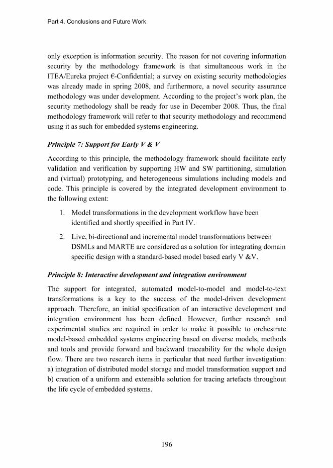
Part 4. Conclusions and Future Work
196
only exception is information security. The reason for not covering information security by the methodology framework is that simultaneous work in the ITEA/Eureka project �-Confidential; a survey on existing security methodologies was already made in spring 2008, and furthermore, a novel security assurance methodology was under development. According to the project�s work plan, the security methodology shall be ready for use in December 2008. Thus, the final methodology framework will refer to that security methodology and recommend using it as such for embedded systems engineering.
Principle 7: Support for Early V & V
According to this principle, the methodology framework should facilitate early validation and verification by supporting HW and SW partitioning, simulation and (virtual) prototyping, and heterogeneous simulations including models and code. This principle is covered by the integrated development environment to the following extent:
1. Model transformations in the development workflow have been identified and shortly specified in Part IV.
2. Live, bi-directional and incremental model transformations between DSMLs and MARTE are considered as a solution for integrating domain specific design with a standard-based model based early V &V.
Principle 8: Interactive development and integration environment
The support for integrated, automated model-to-model and model-to-text transformations is a key to the success of the model-driven development approach. Therefore, an initial specification of an interactive development and integration environment has been defined. However, further research and experimental studies are required in order to make it possible to orchestrate model-based embedded systems engineering based on diverse models, methods and tools and provide forward and backward traceability for the whole design flow. There are two research items in particular that need further investigation: a) integration of distributed model storage and model transformation support and b) creation of a uniform and extensible solution for tracing artefacts throughout the life cycle of embedded systems.

Part 4. Conclusions and Future Work
197
4.4 Lessons Learned
The work for this report was done over a period of nine months, three of which were spent for eliciting and defining requirements for the methodology framework specification work. The authors of this report represent different dimensions that all are specific for embedded systems engineering; hardware vs. software, system engineering vs. software engineering, process vs. architecture, critical systems vs. non-critical systems, etc. Thus, working with this subject required patience from all of us; we had to learn to understand each other, to understand the needs of different application domains, to close the gap in understanding the researchers and engineers who were experts on time-triggered safety critical systems or (mobile) networked systems. As a conclusion, the main difficulty was the definition of a common terminology; it is still evolving while writing this report and it is obvious that there are different interpretations of the terms defined and used.
Although the diversity of our skills has brought challenges in achieving the consensus, it has also been our enrichment. We have had an opportunity to observe embedded systems engineering through the eyes of our colleagues and learn things that are not possible in homogeneous development teams. This will increase these researchers� and engineers� openness to the new things and challenges that will be studied in future ARTEMIS projects in similar kinds of heterogeneous, multi-disciplinary development teams.
The field of embedded systems is broad, its technologies and applications are diverse, and a multitude of design paradigms, languages, methods and tool approaches exist. The authors have also participated in other work activities of the GENESYS project [GENESYS 2008] in order to define the scope of the methodology work and focus on the most important support needs of the cross-domain architecture style and reference architecture template that GENESYS is aiming at. Progressing in parallel, the architecture and methodology related works have, on one hand, had an opportunity to interact proactively. On the other hand, this has caused uncertainties as many issues and options had to be kept open until the last minute.
The cornerstones of the methodology framework are the Y-chart and model- based approach, supporting modelling methods and languages, and a rich set of quality/non-functional property modelling and evaluation methods. The authors think that almost all of the necessary building blocks exist for instantiating whole development processes and environments. However, major advances are

Part 4. Conclusions and Future Work
198
needed to achieve industrial-strength solutions, e.g., interoperability of methods, models and tools should be improved to allow smooth and efficient work, the industrial robustness of many methods and tools should be increased, and the whole methodology framework should be validated by applying it in industry-scale development activities.

199
References [Abdelwahed 2006]
Abdelwahed, S. Notions of Diagnosability for Timed Failure Propagation Graphs. IEEE. 18�21 Sept. 2006. Pp. 643�648.
[Amnell 2003] Amnell, T., Fersman, E., Mokrushin, L., Petterson, P., Yi, W. TIMES: a tool for schedulability analysis and code generationof real-time systems. Proceedings of the 1st International workshop on Formal modelling and analysis of timed systems. FORMATS 2003, Marseille, France, Sep. 6�7, 2003.
[Andrews 2002] Andrews, P. B. An Introduction to Mathematical Logic and Type Theory: To Truth Through Proof. 2nd ed. Kluwer Academic Publishers, available from Springer, 2002.
[ATESST 2007] Advancing Traffic Efficiency and Safety through SoftwareTechnology. Deliverable D2.2.1. Elicitation of representative and relevant analysis and V&V techniques. 2007.
[ATL 2008] Atlas Transformation Language. http://www.eclipse.org/m2m/atl. (2008).
[Baier 2008] Baier, C, Katoen, J.-P. Principles of Model Checking. The MIT Press. 2008.
[Barták 2001] Barták, R. Theory and practice of constraint propagation. In:Proceedings of the 3rd Workshop on Constraint Programming for Decision and Control (CPDC2001), Wydavnictvo PracovniKomputerowej, 2001. Pp. 7�14.
[Bass 2006] Bass, L., Nord, R., Wood, W., Zubrow, D. Risk ThemesDiscovered Through Architecture Evaluations. CMU/SEI-2006-TR-012, 2006. 42 p.

References
200
[Bengtsson 2004]
Bengtsson, P.-O., Lassing, N., Bosch, J., van Vliet, H. Architecture-level modifiability analysis (ALMA). Journal of Systems and Software, 69, 2004, pp. 129�147.
[Bozzano 2003]
Bozzano, M., Villafiorita, A. Improving System Reliability viaModel Checking: The FSAP/NUSMV−SA Safety Analysis Platform. Lecture Notes in Computer Science, ComputerSafety, Reliability, and Security, Vol. 2788/2003. SpringerBerlin/Heidelberg 2003. ISSN 0302-9743. ISBN 978-3-540-20126-7.
[Canal 2008] Canal, C., Poizat P., Salaün, G. Model-based adaptation of behavioural mismatching components. IEEE trans. Software Engineering, 34(4), July�August 2008, pp. 546�563.
[CDO 2008] Eclipse EMF CDO Project Home Page http://www.eclipse.org/modeling/emf/?project=cdo#cdo. (2008).
[Cimatti 1999] Cimatti A. NuSMV: a new symbolic model verifier. Proceeding of International Conference on Computer-Aided Verification(CAV�99). In: Lecture Notes in Computer Science, number1633, Trento, Italy, July 1999. Springer. Pp. 495�499.
[Costagliola 2005]
Costagliola, G., Ferrucci, F., Tortora, G., Vitiello, G. Class Point: An Approach for the Size Estimation of Object-Oriented Systems, IEEE Trans. Software Eng., Vol. 31, No. 1, 2005,pp. 52�74.
[D�Ambrogio 2005]
D�Ambrogio, A. 2005. A Model Transformation Framework forthe Automated Building of Performance Models from UML Models. Fifth International Workshop on Software andPerformance. July 11�15, 2005. Universitat de les Illes Balears. Palma de Mallorca, Spain. Pp. 75�86.
[Davis 2002] Davis, L., Gamble, R. F., Payton, J. The impact of component architectures on interoperability. The Journal of Systems andSoftware 61, 2002, pp. 31�45.
[DECOS 2008] Dependable Embedded Components and Systems. An EUFP6 IP. http://www.decos.at/, Dec. 2008.
References
201
[Douglas 2002] Douglas, B. P. Real-Time Design Patterns: Robust Scalable Architecture for Real-Time Systems. Addison-Wesley, 2002. ISBN 0-201-69956-7.
[EMF 2008] Eclipse Modelling Framework. http://www.eclipse.org/emf, Dec.2008.
[EMMA 2005] European Airport Movement Management by A-SMGCS (EMMA), D681 Recommendations Report, Version 1.0. J. Jakobi (DLR), et al., Braunschweig, 2006.
[Eqyed 1999] Egyed, A., Gacek, C. Automatically Detecting Mismatches during Component-Based and Model-Based Development. 14th IEEE International Conference on Automated Software Engineering, Florida, USA, 1999.
[ESACS 2004] ESACS project. Enhanced Safety Assessment for ComplexSystems. http://www.cert.fr/esacs, Dec. 2008.
[ES 2008] Embedded systems. http://en.wikipedia.org/wiki/Embedded_system#Examples_of_embedded_systems, Dec. 2008.
[Evesti 2008] Evesti, A., Niemelä, E., Henttonen, K., Palviainen, M. A toolchain for quality-driven software architecting. Demonstration in SPLC�08, Limerick, Ireland, 2008.
[FAA 2008] System Safety Handbook. Federal Aviation Administration,May 2008. http://www.faa.gov/, Dec. 2008.
[Falkenhainer 1990]
Falkenhainer, B., Forbus, K. D., Gentner, D. The structure-mapping engine: Algorithm and examples. Artificial Intelligence 41, 1989/90, pp. 1�63.
[Feier 2005] Feier, C., Roman, D., Polleres, A., Domingue, J., Stollberg, M.,Fensel, D. Towards Intelligent Web Services: Web Service Modelling Ontology (WSMO). In: Proc. of the Int�al Conf. on Intelligent Computing (ICIC) 2005, Hefei, China, August 23�26, 2005.
[Fensel 2007] Fensel, D., Lausen, H., Polleres, A., Bruijn, J. D., Stollberg, M.,Roman, D., Domingue, J. Enabling Semantic Web Services.The Web Service Modelling Ontology. 2007, XIV, 41 illus. 188 p.ISBN 978-3-540-34519-0.
References
202
[FIDES 2004] FIDES Guide 2004, Issue A, Reliability Methodology forElectronic Systems, Sept. 2004.
[Fuqua 2005] Fuqua, N. B. Electronic reliability prediction. START, Vol. 4, No. 2. 5 p.
[Gabbay 1994] Gavvay, D. M. Temporal Logic: Mathematical Foundations andComputational Aspects. Oxford University Press. USA, 1994.
[GENESYS 2008]
GENeric Embedded SYStem Platform. http://www.genesys-platform.eu/ (2008).
[Gokhale 2005]
Gokhale, S. S., Lyu, M. R.-T. A simulation approach to structure-based software reliability analysis. IEEE Trans. onSoftware Engineering, Vol. 31, No. 8, 2005, pp. 643�656.
[Goseva-Popstojanova 2001]
Goseva-Popstojanova, K., Trivedi, K. S. Architecture-Based Approach to Reliability Assessment of Software Systems. Performance Evaluation, 45(2�3) 2001, pp. 179�204.
[Hasselbring 2006]
Hasselbring, W., Reussner, R. Troward Trustworthy SoftwareSystems. Computer, April 2006, Vol. 39, No 4, pp. 91�91.
[Henttonen 2007] Henttonen, K., Matinlassi, M., Niemelä, E., Kanstren, T. Integrability and Extensibility Evaluation from Software Architecture Models � A Case Study. Open Software Engineering, Vol. 1, No. 1, 2007, pp. 1�20.
[Holzmann 2003]
Horzmann, G. The SPIN Model Checker: Primer and Reference Manual. Lucent Technologies, 2003.
[IEC IEV 2008]
IEC IEV 191-02-03. http://std.iec.ch/iev/iev.nsf/display?open form&ievref=191-02-03, Dec. 2008.
[IEC-61508]
[IEEE 610.12-1990]
IEC-61508. Functional Safety of Electrical/Electronic/ Programmable Electronic Safety-Related Systems, 2000.
Glossary of Software Engineering Terminology. Institute of Electrical and Electronics Engineers, 01-May-1990. 84 p. ISBN 155937067X.
[IFIP WG 10.4 2008]
http://www.dependability.org/wg10.4/, Dec. 2008.

References
203
[Immonen 2006] Immonen, A. 2006. A method for predicting reliability and availability at the architectural level. In: Software Product-Lines � Research Issues in Engineering and Management. Käkölä, T., Dueñas, J. C. (eds.). Pp. 373�422.
[Immonen 2007] Immonen, A., Palviainen, M. Trustworthiness Evaluation and Testing of Open Source Components. In: 7th International Conference on Quality Software QSIC 2007. Portland, Oregon, 11�12 Oct. 2007. Proc. of 7th International Conference on Quality Software QSIC �07, 2007. Pp. 316�321.
[Immonen 2008] Immonen, A., Evesti, A. Validation of the Reliability Analysis Method and Tool. In: 5th Software Product Lines Testing Workshop (SPLiT 2008), SPLC 2008 Proceedings of the 12th International Software Product Line Conference, 2nd Volume, Limerick, Ireland, 2008. Pp. 163�169.
[Isograph 2008] http://www.isograph.com/workbench.htm, Dec. 2008.
[Jain 1991] Jain, R. 1991. The Art of Computer Systems Performance Analysis: Techniques for Experimental Design, Measurement, Simulation and Modelling. John Wiley & Sons, Inc., 1991. 685 p.
[Jazz 2008] IBM Jazz Platform Information Portal, https://jazz.net/pub/ index.jsp, Dec. 2008.
[Joshi 2005] Joshi, A. Model-Based Safety Analysis Final Report. Internal report. University of Minnesota, 2005.
[Kangas 2006] Kangas, T., Kukkala, P., Orsila, H., Salminen, E., Hännikäinen, M., Hämäläinen, T. D., Riihimäki, J., Kuusilinna, K. UML-based Multi-Processor SoC Design Framework. Transactions on Embedded Computing Systems, Vol. 5, No. 2, ACM, 2006, pp. 281�320.
[Kelly 1999] Kelly, T. P. A Systematic Approach to Safety Case Management. DPhil Thesis, Univ. of York, 1999.
[Kelly 2003] Kelly, T. P. Managing Complex Safety Cases. 11th Safety Critical Systems Symposium (SSS�03), February 2003.
[Keshav 1998] Keshav, R., Gamble, R. Towards a Taxonomy of Architecture Integration Strategies. In: 3rd International Software Architecture Workshop. Florida, Orlando, 1998.
References
204
[Kletz 1992] Kletz, T. HAZOP and HAZAN: Identifying and assessing process industry standards. 3rd ed. Washington, DC: Hemisphere, 1992. ISBN 1-56032-276-4.
[Kreku 2008] Kreku, J., Hoppari, M., Kestilä, T., Qu, Y., Soininen, J.-P., Andersson, P., Tiensyrjä, K. Combining UML2 Application and SystemC Platform Modelling for Performance Evaluation of Real-Time Embedded Systems. EURASIP Journal on Embedded Systems, Vol. 2008, Article ID 712329. 18 p. doi:10.1155/2008/712329.
[Leveson 2000] Leveson, N. G. Intent Specifications: An Approach to Building Human-Centered Specifications. IEEE Transaction on SW Engineering, Vol. 26 (1), 2000.
[Leveson 1991] Leveson, N. G. Software safety in embedded computer systems. Communications of the ACM, Vol. 34, Issue 2, February 1991.
[Leveson 1995] Leveson, N. G. Safeware: System safety and computers. Addison-Wesley Publishing Company, 1995.
[Lieverse 2000] Lieverse, N. G. Intent Specifications: An Approach to Building Human-Centerered Specifications. IEEE Trans. On SW Engineering, Vol. 26 (1), 2000.
[Liu 1973] Liu, C. L., Layland, J. W. Scheduling algorithms for multi-programming in a hard real-time environment. Journal of the ACM, 20, 1973, pp. 46�61.
[Loghi 2004] Loghi, M., Poncino, M., Benini, L. 2004. Cycle-Accurate Power Analysis for Multiprocessor Systems-on-a-Chip. GLSVLSI�04, April 26�28, 2004, Boston, Massachusetts, USA. Pp. 401�406.
[MAST 2008] Modelling and Analysis Suite for real-Time applications. htpp://mast.unican.es/, Dec. 2008.
[MDR 2008] MetaData Repository http://mdr.netbeans.org/, Dec. 2008.
[Medina 2005] Medina, J. Metodología y Herramientas UML para el Medelado y Analisis de Sistemas de Tiempo Real Orientados a Objetos. PhD Thesis, 2005.
References
205
[Mili 2000] Mili, R., Desharnais, J., Frappier, M., Mili, A. Semantic distance between specifications. Theoretical Computer Science 247, 2000, pp. 257�276.
[Nicholson 2000] Nicholson, M., Conmy, P. et al. Generating and maintaining a Safety Argument for Integrated Modular Systems. 5th Australian Workshop on Safety Critical Systems and Software. Australia, 2000.
[Niemelä 2007] Niemelä, E., Immonen, A. 2007. Capturing quality requirements of product family architecture. Information and Software Technology. 49 (11�12), 2007, pp. 1107�1120.
[Niemelä 2008] Niemelä, E., Evesti, A., Savolainen, P. Modelling Quality Attribute Variability. Third International Conference on Evaluation of Novel Approaches of Software Engineering, ENASE 2008, Funchal, Madeira, Portugal, May 4�7, 2008. Pp. 169�176.
[Obermaisser 2005]
Obermaisser, R. Event-Triggered and Time-Triggered Control Paradigms � An Integrated Architecture. Springer-Verlag, Hardcover, Real-Time Systems Series, Vol. 22, 2005. ISBN 0387230432. 170 p.
[Ocarina 2008] An AADL model processing suite. http://ocarina.enst.fr/, Dec. 2008.
[OMG 2008] OMG. MARTE (Modeling and Analysis of Real-time and Embedded systems). http://www.omgmarte.org/, Dec. 2008.
[OWL 2008] OWL-S. http://www.ai.sri.com/daml/services/owl-s/1.2/, Dec. 2008.
[Palviainen 2008] Palviainen, M., Evesti, A., Niemelä, E. Integrated Approach for Reliability Evaluation and the Testing of Open Source based Software Systems. Submitted to Software: Practice and Experience. 28 p.
[Papadopoulos 1999]
Papadopoulos, Y., McDermid. J. A. Hierarchically Performed Hazard Origin and Propagation Studies. SAFECOMP 1999. Pp. 139�152.
[Pataricza 2006] Pataricza, A. Model-based dependability analysis. DSc Thesis, Hungarian Academy of Sciences, 2006.

References
206
[Paul 2005] Paul, J. M., Thomas, D. E., Cassidy, A. S. High-Level Modelling and Simulation of Single-Chip Programmable Heterogeneous Multiprocessors. ACM Transactions on Design Automation of Electronic Systems, Vol. 10, No. 3, 2005, pp. 431�461.
[Petriu 2008] Petriu, D. B. 2008. Performance Analysis with MARTE and PUMA. Available at: http://www.omg.org/docs/omg/08-06-35.pdf, Dec. 2008.
[Pimentel 2006] Pimentel, A., Erbas, C. A Systematic Approach to Exploring Embedded System Architectures at Multiple Abstraction Levels. IEEE Transactions on Computers, Vol. 55, No. 2, Feb. 2006, pp. 99�112.
[PRISM 1999] PRIMS, �System Reliability Assessment Software Tool�. Reliability Analysis Center (RAC), 1999.
[Purhonen 2004] Purhonen, A. Performance optimization of embedded software architecture � a case study. 4th Working IEEE/IFIP Conference on Software Architecture, WICSA 2004, 12�15 June 2004 Oslo, Norway. IEEE Computer Society (2004). Pp. 112�121.
[ReliaSoft 2008] http://www.reliasoft.com/predict/features.htm, Dec. 2008.
[Reussner 2003] Reussner, R. H., Schmidt, H. W., Poernomo, I. H. Reliability prediction for component-based software architectures. The Journal of Systems and Software, 66(2003), pp. 241�252.
[Rodriques 2005a]
Rodrigues, G. N., Rosenblum, D. S., Uchitel, S. 2005. Reliability Prediction in Model-Driven Development. MoDELS 2005, Briand, L., Williams, C. (Eds.), LNCS 3713. Pp. 339�353.
[Rodriques 2005b]
Rodrigues, G. N., Rosenblum, D., Uchitel, S. Sensitivity Analysis for a Scenario-Based Reliability Prediction Model. ICSE 2005 Workshop on architecting Dependable Systems, 2005. Pp. 73�77.
[Rushby 1993] Rushby, J. Formal Methods and Digital Systems Validation for Airborne Systems, SRI-CSL-93-07, 1993.
[Sha 1990] Sha, L., Rajkumar, R., Lehoczky, J. P. Priority inheritance protocols: An approach to real-time synchronization. IEEE Trans. on Computers, 1990.

References
207
[Shariful 2006] Islam, M. S., Csertán, G., Balogh, A., Herzner, W., LeSergent, T., Pataricza, A., Suri, N. SW-HW Integration Process for the Generation of Platform Specific Models. In: Publications of the Austrian Electrotechnical Association: Proc. of the Informationstagung Mikroelektronik ME 2006. Vienna, Austria 2006. Pp. 194�203.
[Simunic 2001] Simunic, T., Benini, L., De Micheli, G. Energy-Efficient Design of Battery-Powered Embedded Systems. IEEE TVLSI, Vol. 9, No. 1, February 2001, pp. 15�28.
[Singhoff 2004] Singhoff, F., Legrand, J., Nana, L., Marcé, L. Cheddar: A flexible real-time scheduling framework. ACM SIGAda Ada Letters, Vol. 24, No. 4, 2004, pp. 1�8.
[Tarvainen 2008] Tarvainen, P. 2008. Adaptability Evaluation at Software Architecture Level. The Open Software Engineering Journal, Vol. 2, No. 1, 2008, pp. 1�30. doi:10.2174/1874107X00802010001.
[Tindell 1994a] Tindell, K., Clark, J. Holistic schedulability analysis for distributed hard real-time systems. Microprocessing & Microprogramming, Vol. 50, No. 2�3, 1994, pp. 117�134.
[Tindell 1994b] Tindell, K. Adding time-offsets to schedulability analysis. Technical Report YCS 221, Dept. of computer science, University of York, England, 1994.
[Tsang 1993] Tsang, E. Foundations of constraint satisfaction. Academic Press. 1993.
[Tsantalis 2006] Tsantali, N., Chatzigeorgiou, A., Stephanides, G., Halkidis, S. Design pattern detection using similarity scoring. IEEE Trans. Software Engineering, 32(11), Nov. 2006, pp. 896�909.
[Varró 2004] Varró, D. Automated Model Transformations for the Analysis of IT Systems. PhD thesis. Budapest University of Technology and Economics, 2004.
[Venkatachalam 2005]
Venkatachalam, V., Franz, M. Power reduction techniques for microprocessor systems. ACM Computing Surveys (CSUR), Vol. 37, Issue 3 (September 2005), pp. 195�237.
[VIATRA 2008]
VIATRA2 Model Transformation Framework, http://www. eclipse.org/gmt, Dec. 2008.
References
208
[Wild 2006] Wild, T., Herkersdorf A., Lee, G.-Y. TAPES � Trace-based architecture performance evaluation with SystemC. Design Automation for Embedded Systems, Vol. 10, Numbers 2�3, Special Issue on SystemC-based System Modelling, Verification and Synthesis, 2006. Pp. 157�179.
[Woodside 2005]
Woodside, M., Petriu, D. C., Petriu D. B., Shen, H., Israr, T., Merseguer, J. 2005. Performance by Unified Model Analysis (PUMA). Fifth International Workshop on Software and Performance. July 11�15, 2005. Universitat de les Illes Balears. Palma de Mallorca, Spain. Pp. 1�12.

Series title, number and report code of publication
VTT Publications 705 VTT-PUBS-705
Author(s) Eila Ovaska, András Balogh, Sergio Campos, Adrian Noguero, András Pataricza, Kari Tiensyrjä & Josetxo Vicedo Title
Model and Quality Driven Embedded Systems Engineering
Abstract The world of embedded systems is broad and diverse, addressing a wide variety of application domains. Although technologically, the situation for embedded systems is still quite fragmented, platform-based engineering, reference designs and maturing system domains have effected great changes. However, the features of modern embedded systems are changing at such a rate that it is increasingly difficult for companies to bring new products to the market within acceptable time scales and still guarantee acceptable levels of operational quality. This report aims for its part to increase the convergence of views with regard to embedded systems technologies and engineering methods.
The objective of this report is to introduce the methodology framework for model and quality driven embedded systems engineering. The framework is composed of three key artefacts, which provide the basis for building specific methodology instances. While instantiating this methodology framework, it has to be adapted to the needs and constraints of that specific application domain and development organisation.
The first key artefact of the methodology framework is the process model, the Y-chart model. The second key artefact is the Unified Modelling Language (UML) adapted to embedded systems engineering with a specific profile. The third key artefact consists of a set of evaluation methods that have been selected for use in embedded system engineering. Within the conclusions, an initial integrated development environment is introduced for embedded systems engineering. The methods selected for the methodology framework have been validated in different application domains of embedded or/and software systems engineering areas.
ISBN 978-951-38-7336-3 (URL: http://www.vtt.fi/publications/index.jsp)
Series title and ISSN Project number
VTT Publications 1455-0849 (URL: http://www.vtt.fi/publications/index.jsp)
18985
Date Language Pages February 2009 English 208 p.
Name of project Commissioned by Genesys EU
Keywords Publisher methodology, modelling, evaluation, quality, embedded systems engineering
VTT Technical Research Centre of Finland P.O. Box 1000, FI-02044 VTT, Finland Phone internat. +358 20 722 4520 Fax +358 20 722 4374

Modeling Process
Applicationrequirements
SystemrequirementsSpecification(1)
Platformrequirements
Referencearchitecturetemplate
Platformmodule library
Platformarchitecturedesign (3)
Cross-domainarchitecturestyle
Applicationarchitecturedesign (2)
Applicationservice
repository
System allocation/configuration/ refinement (4)
Qualityevaluation (5)
Realization(HW/SW)(6)
Evaluationcriteria
Validated systemArchitecture
models
VTT PUBLICATIONS 705VTT CREATES BUSINESS FROM TECHNOLOGY Technology and market foresight • Strategic research • Product and service development • IPR and licensing • Assessments, testing, inspection, certifi cation • Technology and innovation management • Technology partnership
• • • VTT PUB
LICA
TION
S 705 MO
DEL A
ND
QU
ALITY D
RIVEN
EMB
EDD
ED SYSTEM
S ENG
INEER
ING
ISBN 978-951-38-7336-3 (URL: http://www.vtt.fi /publications/index.jsp)ISSN 1455-0849 (URL: http://www.vtt.fi /publications/index.jsp)
Eila Ovaska, András Balogh, Sergio Campos, Adrian Noguero, András Pataricza, Kari Tiensyrjä & Josetxo Vicedo
Model and Quality Driven Embedded Systems Engineering
VTT PUBLICATIONS
692 Kimmo Keränen. Photonic module integration based on silicon, ceramic and plastic technologies. 2008. 101 p. + app. 70 p.
693 Emilia Selinheimo. Tyrosinase and laccase as novel crosslinking tools for food biopolymers. 2008. 114 p. + app. 62 p.
694 Olli-Pekka Puolitaival. Adapting model-based testing to agile context. 2008. 69 p. + app. 6 p.
695 Minna Pikkarainen. Towards a Framework for Improving Software Development Process Mediated with CMMI Goals and Agile Practices. 2008. 119 p. + app. 193 p.
696 Suvi T. Häkkinen. A functional genomics approach to the study of alkaloid biosynthesis and metabolism in Nicotiana tabacum and Hyoscyamus muticus cell cultures. 2008. 90 p. + app. 49 p.
697 Riitta Partanen. Mobility and oxidative stability in plasticised food matrices. The role of water. 2008. 92 p. + app. 43 p.
698 Mikko Karppinen. High bit-rate optical interconnects on printed wiring board. Micro-optics and hybrid integration. 2008. 162 p.
699 Frej Wasastjerna. Using MCNP for fusion neutronics. 2008. 68 p. + app. 136 p.
700 Teemu Reiman, Elina Pietikäinen & Pia Oedewald. Turvallisuuskulttuuri. Teoria ja arviointi. 2008. 106 s.
701 Pekka Pursula. Analysis and Design of UHF and Millimetre Wave Radio Frequency Identifi cation. 2008. 82 p. + app. 51 p.
702 Leena Korkiala-Tanttu. Calculation method for permanent deformation of unbound pavement materials. 2008. 92 p. + app. 84 p.
703 Lauri Kurki & Ralf Marbach. Radiative transfer studies and Next-Generation NIR probe prototype. 2009. 43 p.
704 Anne Heikkilä. Multipoint-NIR-measurements in pharmaceutical powder applications. 2008. 60 p.
705 Eila Ovaska, András Balogh, Sergio Campos, Adrian Noguero, András Pataricza, Kari Tiensyrjä & Josetxo Vicedo. Model and Quality Driven Embedded Systems Engineering. 2009. 208 p.