User Guide to

MODDE

By MKS Umetrics

Version 11

1992-2015 MKS Umetrics AB, all rights reserved Information in this document is subject to change without notice and does not represent a commitment on part of MKS Umetrics. The software, which includes information contained in any databases, described in this document is furnished under license agreement or nondisclosure agreement and may be used or copied only in accordance with the terms of the agreement. It is against the law to copy the software except as specifically allowed in the license or nondisclosure agreement. No part of this user guide may be reproduced or transmitted in any form or by any means, electronic or mechanical, including photocopying and recording, for any purpose, without the express written permission of MKS Umetrics.

MKS Umetrics patents and trademarks:

SEQUENTIAL MODELING, US-7523384

MONITORING MULTIVARIATE PROCESSES, US-5949678

TOP-DOWN CLUSTERING/PLS-TREE®, US-8244498

DESIGN SPACE, US-8086327

MPMC, Pending

COMPUTER-IMPLEMENTED SYSTEMS AND METHODS FOR GENERATING GENERALIZED FRACTIONAL DESIGNS, Pending

RED-MUP®, VALUE FROM DATA®, OPLS®, O2PLS®, OPLS-DA®, O2PLS-DA®, PLS-TREE®, S-PLOT®, EZinfo®, FABSTAT®, SIMCA®. MODDE®

ID #2056

User guide edition date: May 19, 2015

MKS Umetrics AB Stortorget 21

SE-211 34 Malmö Sweden

Phone: +46 (0)40 664 2580

Email: info@umetrics.com

Welcome

Welcome to the user guide for MODDE 11.

This is your guide to MODDE and its capabilities. It explains how to install and use MODDE.

Content

This user guide is divided into 14 chapters, 5 appendices and one reference list. Chapter 1 gives a short introduction of how to use MODDE. Chapter 2 presents an introduction to experimental design. Chapters 3 - 14 provide step-by-step procedures for creating and using experimental designs with MODDE.

The Statistical appendix presents short explanations of statistical methods used by MODDE.

The Design appendix presents short descriptions of the designs available in MODDE.

The Optimizer appendix describes the optimizer feature and the properties of the different optimizer objectives.

The Design space appendix describes the design space estimation feature.

The Stability design appendix describes how to create and work with a stability design in MODDE.

References are available on the references page.

v

Table of contents 

01-Getting started 1 Introduction.................................................................................................................... 1 Installation ..................................................................................................................... 1 Starting MODDE ........................................................................................................... 2 

Getting help ......................................................................................................................... 2 Tutorials .............................................................................................................................. 2 Starting a new investigation ................................................................................................ 2 

Experimental cycle ........................................................................................................ 2 Design phase .................................................................................................................. 2 Analysis phase ............................................................................................................... 2 

Explore the data .................................................................................................................. 3 Evaluate the design ............................................................................................................. 3 Fit ........................................................................................................................................ 3 Review the fit using plots and lists ...................................................................................... 3 Diagnostics .......................................................................................................................... 3 Interpret the model .............................................................................................................. 3 Refine the model ................................................................................................................. 4 

Prediction phase (using the model) ................................................................................ 4 Help ............................................................................................................................... 4 

MODDE Help ..................................................................................................................... 4 Registration and activation .................................................................................................. 5 MKS Umetrics on the Web ................................................................................................. 5 About MODDE ................................................................................................................... 5 

Using MODDE .............................................................................................................. 6 MODDE ribbon description ................................................................................................ 6 License information ............................................................................................................ 7 Keyboard shortcuts .............................................................................................................. 7 Mini toolbar ........................................................................................................................ 8 Quick access toolbar ........................................................................................................... 9 Customizing the user interface .......................................................................................... 10 Investigation ...................................................................................................................... 10 

02-Introduction 13 General description ...................................................................................................... 13 What is modeling and experimental design? ............................................................... 13 Objectives of modeling and experimental design ........................................................ 13 Screening models and designs ..................................................................................... 13 

Number of factors in screening designs ............................................................................ 14 Number of factors with split objective .............................................................................. 14 

Response surface modeling (RSM) designs ................................................................. 14 Number of factors in RSM designs ................................................................................... 14 Number of factors in split objective .................................................................................. 14 

Fit methods .................................................................................................................. 15 Multiple Linear Regression (MLR) ................................................................................... 15 Partial Least Squares (PLS) ............................................................................................... 15 

MODDE 11

vi

Results ............................................................................................................................... 16 Analysis phase ............................................................................................................. 16 

Review the model fit ......................................................................................................... 16 Assess model adequacy ..................................................................................................... 17 

Prediction - using the fitted model ............................................................................... 17 Conventions ................................................................................................................. 17 

Limitations in investigation names .................................................................................... 17 Limitations in factor and response names ......................................................................... 17 Case sensitivity ................................................................................................................. 17 Menu and tab reference syntax .......................................................................................... 18 Select and mark ................................................................................................................. 18 Vector and matrix representation ...................................................................................... 18 

Suggestions for further reading on experimental designs ............................................ 19 

03-Design wizard 21 Introduction.................................................................................................................. 21 Factors ......................................................................................................................... 21 

Factor definition dialog box .............................................................................................. 22 General tab ........................................................................................................................ 23 Advanced .......................................................................................................................... 26 

Constraints ................................................................................................................... 28 Defining constraints .......................................................................................................... 28 Defining constraints in the spreadsheet ............................................................................. 28 Constraints supported ........................................................................................................ 29 Constraints in qualitative or quantitative multilevel factors .............................................. 29 

Responses .................................................................................................................... 30 Defining responses ............................................................................................................ 30 Response definition dialog box ......................................................................................... 30 Regular responses ............................................................................................................. 31 MLR scaling ...................................................................................................................... 32 PLS scaling ....................................................................................................................... 32 Derived responses ............................................................................................................. 32 Linked responses ............................................................................................................... 35 

Objective ...................................................................................................................... 35 Select objective ................................................................................................................. 35 

Model and design ......................................................................................................... 37 Selecting model and design ............................................................................................... 37 Design runs ....................................................................................................................... 39 Center points ..................................................................................................................... 39 Replicates .......................................................................................................................... 39 Total runs .......................................................................................................................... 39 Blocks ............................................................................................................................... 40 Settings .............................................................................................................................. 40 How high should the power be? ........................................................................................ 41 

D-Optimal .................................................................................................................... 41 D-Optimal pages ............................................................................................................... 41 Design generation criteria section ..................................................................................... 41 Design alternatives section ................................................................................................ 42 Candidate set section ......................................................................................................... 43 D-Optimal results .............................................................................................................. 44 D-Optimal onion pages ..................................................................................................... 45 Onion on the Design tab .................................................................................................... 47 

Table of Contents

vii

Reduced combinatorial ................................................................................................ 47 Design generation options ................................................................................................. 47 Reduced combinatorial design selection page ................................................................... 48 

04-File 51 Introduction.................................................................................................................. 51 Info............................................................................................................................... 52 

Protect investigation .......................................................................................................... 52 Report ................................................................................................................................ 54 

New .............................................................................................................................. 55 Experimental design .......................................................................................................... 55 Using existing design ........................................................................................................ 55 Specific application design ................................................................................................ 60 

Open ............................................................................................................................. 63 Recent investigations ........................................................................................................ 64 Recent folders ................................................................................................................... 64 Browse .............................................................................................................................. 64 

Save ............................................................................................................................. 64 Save as ......................................................................................................................... 64 

Save plot as ....................................................................................................................... 64 Save list as ......................................................................................................................... 65 Save or Copy a plot ........................................................................................................... 65 

Print ............................................................................................................................. 67 Send ............................................................................................................................. 67 

Send as attachment ............................................................................................................ 67 Close ............................................................................................................................ 68 Options ......................................................................................................................... 68 

MODDE options ............................................................................................................... 68 Investigation options ......................................................................................................... 70 

Audit trail ..................................................................................................................... 73 Coefficients .................................................................................................................. 74 

Scaled and centered coefficients ....................................................................................... 74 Orthogonal coefficients in PLS ......................................................................................... 74 Unscaled ............................................................................................................................ 74 Normalized coefficients .................................................................................................... 74 Confidence interval ........................................................................................................... 75 Extended or compact format ............................................................................................. 75 Interval type and probability levels ................................................................................... 75 

Residuals ...................................................................................................................... 76 Raw residuals .................................................................................................................... 76 Standardized residuals ....................................................................................................... 77 Deleted studentized residuals ............................................................................................ 77 Customize ribbon .............................................................................................................. 78 Customize quick access toolbar ........................................................................................ 79 Keyboard shortcuts ............................................................................................................ 79 Restore .............................................................................................................................. 81 

Help ............................................................................................................................. 81 Activate MODDE ............................................................................................................. 82 View help .......................................................................................................................... 82 MKS Umetrics on the Web ............................................................................................... 82 Knowledge base ................................................................................................................ 82 About us ............................................................................................................................ 82 

MODDE 11

viii

05-Home 83 Introduction.................................................................................................................. 83 Design wizard .............................................................................................................. 84 Analysis wizard ........................................................................................................... 84 

Replicates .......................................................................................................................... 85 Histogram .......................................................................................................................... 86 Summary of Fit ................................................................................................................. 88 Coefficients ....................................................................................................................... 89 Residuals Normal Probability ........................................................................................... 92 Observed vs. Predicted ...................................................................................................... 93 

Specification ................................................................................................................ 93 Spreadsheet access ............................................................................................................ 94 

Edit model .................................................................................................................... 94 Edit Model dialog box ....................................................................................................... 94 Model list .......................................................................................................................... 95 

Fit model ...................................................................................................................... 96 Standard fit ........................................................................................................................ 96 Mixture fit ......................................................................................................................... 97 

Summary of fit ............................................................................................................. 97 Overview ..................................................................................................................... 99 Coefficients ................................................................................................................ 100 Residuals .................................................................................................................... 100 Observed vs. predicted ............................................................................................... 100 

Properties ........................................................................................................................ 101 Contour ...................................................................................................................... 101 Sweet spot .................................................................................................................. 102 Design space .............................................................................................................. 102 Optimizer ................................................................................................................... 103 Exclude ...................................................................................................................... 103 Undo .......................................................................................................................... 103 

06-Design 105 Introduction................................................................................................................ 105 Factors ....................................................................................................................... 106 

Factors spreadsheet ......................................................................................................... 106 Responses .................................................................................................................. 108 

Responses spreadsheet .................................................................................................... 108 Constraints ................................................................................................................. 109 

Specifying constraints ..................................................................................................... 109 Defining a constraint graphically .................................................................................... 110 Modifying a constraint graphically ................................................................................. 110 Candidate set with a constraint ........................................................................................ 111 

Inclusions ................................................................................................................... 111 Opening the inclusions spreadsheet ................................................................................. 111 Inclusions vs. complement design ................................................................................... 111 Adding inclusions to the worksheet ................................................................................ 112 Inclusions as part of the design ....................................................................................... 112 Editing inclusions ............................................................................................................ 113 

Reference mixture ...................................................................................................... 113 Generators .................................................................................................................. 114 

Table of Contents

ix

Objective .................................................................................................................... 115 Design region ............................................................................................................. 115 

Design region properties ................................................................................................. 116 Design matrix ............................................................................................................. 116 Design matrix for Stability designs ............................................................................ 117 

Overview tab ................................................................................................................... 117 All tab ............................................................................................................................. 118 A, B, C etc. tabs .............................................................................................................. 118 

Design summary ........................................................................................................ 119 Design summary D-Optimal ...................................................................................... 119 Design summary, Stability designs ............................................................................ 121 Confoundings ............................................................................................................. 122 

To list the confoundings .................................................................................................. 122 Candidate set .............................................................................................................. 123 

Accessing the Candidate set ............................................................................................ 123 New design ................................................................................................................ 124 

New D-Optimal design ................................................................................................... 124 Select from already generated D-Optimal designs .......................................................... 124 

Onion ......................................................................................................................... 124 Onion Plot ....................................................................................................................... 124 Onion 3D Plot ................................................................................................................. 125 

07-Worksheet 127 Introduction................................................................................................................ 127 Worksheet .................................................................................................................. 128 

Accessing the Worksheet ................................................................................................ 128 Description of the worksheet ........................................................................................... 128 Missing values in the worksheet ..................................................................................... 128 Deleting the worksheet .................................................................................................... 129 Adding experiments in the worksheet ............................................................................. 129 Sorting the worksheet ...................................................................................................... 129 Colors in the worksheet ................................................................................................... 129 

Sorting spreadsheet .................................................................................................... 129 Custom sort ..................................................................................................................... 129 Sorting the candidate set ................................................................................................. 130 

Scatter ........................................................................................................................ 130 Run order ................................................................................................................... 131 

Randomize run order ....................................................................................................... 131 Run order to detect curvature .......................................................................................... 131 Curvature diagnostics plot ............................................................................................... 131 

Correlation ................................................................................................................. 133 Descriptive statistics .................................................................................................. 134 

Descriptive statistics properties ....................................................................................... 136 Box Whisker .............................................................................................................. 136 Histogram .................................................................................................................. 137 

Accessing the Histogram ................................................................................................. 137 Replicates ................................................................................................................... 138 

Accessing the Replicate plot ........................................................................................... 138 Plot information .............................................................................................................. 138 

MODDE 11

x

08-Analyze 141 Introduction................................................................................................................ 141 Summary of fit ........................................................................................................... 141 

Summary of fit plot ......................................................................................................... 143 PLS total summary plot ................................................................................................... 143 PLS response summary plot ............................................................................................ 144 Summary of fit list .......................................................................................................... 145 PLS summary list ............................................................................................................ 145 

ANOVA ..................................................................................................................... 146 ANOVA table ................................................................................................................. 146 ANOVA plot ................................................................................................................... 147 

Lack of fit .................................................................................................................. 148 Box-Cox plot (MLR only) ......................................................................................... 149 Residuals .................................................................................................................... 150 

Residual type ................................................................................................................... 151 Residuals normal probability plot ................................................................................... 151 Residuals vs. predicted response ..................................................................................... 152 Residuals vs. run order .................................................................................................... 153 Residuals vs. variable ...................................................................................................... 153 Residuals list ................................................................................................................... 154 

Observed vs. predicted ............................................................................................... 154 Properties ........................................................................................................................ 155 

Coefficients ................................................................................................................ 155 Coefficient plot ............................................................................................................... 156 Coefficient overview plot ................................................................................................ 157 Coefficient list ................................................................................................................. 158 Coefficient overview list ................................................................................................. 158 

Effects ........................................................................................................................ 159 Accessing effects plots and list ....................................................................................... 159 Effect plot ........................................................................................................................ 159 Effects normal probability plot ........................................................................................ 160 Main effect plot ............................................................................................................... 161 Effect list ......................................................................................................................... 162 

Interactions ................................................................................................................ 163 PLS ............................................................................................................................ 163 

Score plots ....................................................................................................................... 164 Loading plots................................................................................................................... 164 

Distance to model (Y) ................................................................................................ 165 VIP - Variable importance in the projection .............................................................. 166 

09-Predict 169 Introduction................................................................................................................ 169 Prediction spreadsheet ............................................................................................... 170 Prediction scatter plot ................................................................................................ 170 Prediction plots .......................................................................................................... 171 

Prediction plot ................................................................................................................. 172 Overlay prediction plot ................................................................................................... 172 

Factor effects ............................................................................................................. 173 Factor effects, Stability designs ................................................................................. 174 Contour ...................................................................................................................... 175 

2D contour ...................................................................................................................... 175 

Table of Contents

xi

4D contour ...................................................................................................................... 176 Response surface ............................................................................................................. 177 Contour plot wizard......................................................................................................... 178 Contour plot options ........................................................................................................ 180 

Sweet spot .................................................................................................................. 180 Creating a sweet spot plot ............................................................................................... 181 

Design space .............................................................................................................. 184 Design space wizard .................................................................................................. 185 

First page ......................................................................................................................... 185 4D axes............................................................................................................................ 186 

Optimizer ................................................................................................................... 187 Setpoint validation ..................................................................................................... 187 

Setpoint validation plots and lists .................................................................................... 188 

10-View 189 Introduction................................................................................................................ 189 Show .......................................................................................................................... 189 Audit trail ................................................................................................................... 190 Favorites .................................................................................................................... 191 

Introduction ..................................................................................................................... 191 Full screen .................................................................................................................. 193 Window ..................................................................................................................... 193 

Close ............................................................................................................................... 193 Switch windows .............................................................................................................. 194 

11-Tools 195 Introduction................................................................................................................ 195 Add plot element ........................................................................................................ 195 

Available plot elements ................................................................................................... 196 Templates ................................................................................................................... 196 Select ......................................................................................................................... 197 

Free-form selection ......................................................................................................... 197 Rectangular selection ...................................................................................................... 197 Select along the X-axis .................................................................................................... 197 Select along the Y-axis .................................................................................................... 198 Move points .................................................................................................................... 198 

Zoom and zoom out ................................................................................................... 198 Zoom and rotate 3D plots ................................................................................................ 198 

Screen reader ............................................................................................................. 199 Exclude ...................................................................................................................... 199 Format plot................................................................................................................. 199 

Accessing format plot ..................................................................................................... 199 Mini toolbar .................................................................................................................... 200 Axis ................................................................................................................................. 200 Axis Font and Title Font ................................................................................................. 201 Gridlines .......................................................................................................................... 202 Background ..................................................................................................................... 202 Titles and Font ................................................................................................................ 203 Legend and Font .............................................................................................................. 203 Limits and regions ........................................................................................................... 203 Labels .............................................................................................................................. 204 

MODDE 11

xii

Contour ........................................................................................................................... 204 Error bars ........................................................................................................................ 205 Column ............................................................................................................................ 205 Styles ............................................................................................................................... 205 

List ............................................................................................................................. 206 Add to favorites ......................................................................................................... 206 Add to report .............................................................................................................. 206 Plots and lists ............................................................................................................. 206 

Properties dialog box ....................................................................................................... 206 Automatic update of plots and lists ................................................................................. 206 Generating multiple plots or lists .................................................................................... 206 

12-Optimizer 207 Introduction................................................................................................................ 207 

Starting the optimizer ...................................................................................................... 207 Optimizer theory ............................................................................................................. 207 Optimizer objectives ....................................................................................................... 208 

Optimizer window ..................................................................................................... 208 Objective tab ................................................................................................................... 210 Optimizer desirability ...................................................................................................... 211 Factor spreadsheet ........................................................................................................... 213 CCC constraints .............................................................................................................. 213 Setpoint tab ..................................................................................................................... 214 Alternative setpoints tab .................................................................................................. 215 Optimizer list................................................................................................................... 218 

Optimizer tab ............................................................................................................. 219 Dynamic profile .............................................................................................................. 220 Creating contour plots from the optimizer ...................................................................... 220 Contour plot wizard from the optimizer .......................................................................... 221 Creating a sweet spot plot from the optimizer ................................................................. 221 Sweet spot plot wizard from the optimizer ...................................................................... 222 Creating a design space plot from the optimizer ............................................................. 223 Design space wizard from the optimizer ......................................................................... 223 Find robust setpoint ......................................................................................................... 225 Setpoint analysis ............................................................................................................. 228 

13-Setpoint 229 Introduction................................................................................................................ 229 Setpoint analysis plots and lists ................................................................................. 229 Setpoint window ........................................................................................................ 230 

Preventing auto update .................................................................................................... 230 Adding more columns ..................................................................................................... 230 Setpoint properties .......................................................................................................... 230 Response spreadsheet ...................................................................................................... 233 

Factor distribution ...................................................................................................... 234 Response distribution ................................................................................................. 235 Setpoint summary ...................................................................................................... 235 Individual response analysis ...................................................................................... 235 Setpoint, design space ................................................................................................ 236 

Table of Contents

xiii

14-Report 237 Introduction................................................................................................................ 237 Opening the Report generator .................................................................................... 237 Saving a report ........................................................................................................... 238 Opening and saving an old report .............................................................................. 238 Report window ........................................................................................................... 239 File tab ....................................................................................................................... 239 

General Windows commands .......................................................................................... 239 Save as ............................................................................................................................ 240 

Home ......................................................................................................................... 240 Introduction ..................................................................................................................... 240 Clipboard ......................................................................................................................... 241 Font and Paragraph ......................................................................................................... 241 Insert ............................................................................................................................... 241 Report .............................................................................................................................. 241 Formatting ....................................................................................................................... 242 

View tab ..................................................................................................................... 242 Placeholders window ................................................................................................. 243 Properties window ..................................................................................................... 244 Adding plots and lists to the report ............................................................................ 244 

Statistical appendix 245 Introduction................................................................................................................ 245 Fit methods ................................................................................................................ 245 

Multiple linear regression (MLR) ................................................................................... 245 Partial least squares regression (PLS) ............................................................................. 246 Cross-validation significance rules.................................................................................. 248 Model .............................................................................................................................. 249 Hierarchy ......................................................................................................................... 249 

Scaling ....................................................................................................................... 249 Scaling the factor matrix, X ............................................................................................ 249 Scaling the response matrix, Y ........................................................................................ 250 

Missing data ............................................................................................................... 250 Missing data in the design matrix, X ............................................................................... 250 Missing data in Y with multiple linear regression ........................................................... 250 Missing data in Y with PLS regression ........................................................................... 250 

Number of observations ............................................................................................. 251 Summary of fit ........................................................................................................... 251 

R2 .................................................................................................................................... 251 Q2.................................................................................................................................... 251 Model validity ................................................................................................................. 252 Reproducibility ................................................................................................................ 252 

Residual standard deviation (RSD) ............................................................................ 252 Analysis of variance, ANOVA .................................................................................. 252 Measures of goodness-of-fit ...................................................................................... 253 

Q2.................................................................................................................................... 253 R2 .................................................................................................................................... 254 Adjusted R2 .................................................................................................................... 254 F-test ............................................................................................................................... 255 Degrees of freedom and saturated models ....................................................................... 255 

MODDE 11

xiv

Coefficients ................................................................................................................ 256 Scaled and centered coefficients ..................................................................................... 256 Orthogonal coefficients in PLS ....................................................................................... 256 Unscaled .......................................................................................................................... 256 Normalized coefficients .................................................................................................. 256 Confidence interval ......................................................................................................... 256 Extended or compact format ........................................................................................... 257 

Analysis wizard tests ................................................................................................. 257 Qualitative factors with more than 2 levels ............................................................... 258 Residuals .................................................................................................................... 258 

Raw residuals .................................................................................................................. 258 Standardized residuals ..................................................................................................... 258 Deleted studentized residuals .......................................................................................... 258 

Condition number ...................................................................................................... 259 Condition number definition ........................................................................................... 259 Condition number with mixture factors........................................................................... 260 PLS and Cox reference mixture model ........................................................................... 260 MLR regression and the Cox reference mixture model ................................................... 260 MLR and Scheffé models ................................................................................................ 260 

Interval estimates ....................................................................................................... 261 PLS plots .................................................................................................................... 262 

Loadings - WC plots ....................................................................................................... 262 Scores - TT, UU, and TU plots ....................................................................................... 263 

PLS regression coefficients ....................................................................................... 263 Box-Cox plot (only MLR) ......................................................................................... 263 Mixture data in MODDE ........................................................................................... 264 Mixture factors only, Model types ............................................................................. 264 

Slack variable model ....................................................................................................... 265 Cox reference mixture model .......................................................................................... 265 Scheffé model ................................................................................................................. 265 

Mixture factors only, fitting a model ......................................................................... 265 Analysis and fit method................................................................................................... 265 MLR and the Cox reference mixture model .................................................................... 267 PLS and the Cox reference mixture................................................................................. 267 Scheffé models derived from the Cox reference mixture model ..................................... 268 Scheffé models ................................................................................................................ 268 Using the model .............................................................................................................. 269 

Process and mixture factors ....................................................................................... 269 MODDE plots ................................................................................................................. 269 

Optimizer ................................................................................................................... 269 Desirability ...................................................................................................................... 270 Overall desirability .......................................................................................................... 273 Overall distance to target ................................................................................................. 273 Starting simplexes ........................................................................................................... 274 Sensitivity analysis .......................................................................................................... 274 Factor contribution .......................................................................................................... 275 

Orthogonal blocking .................................................................................................. 276 Blocking screening designs ............................................................................................. 277 Blocking RSM designs .................................................................................................... 278 Blocking D-Optimal designs ........................................................................................... 279 Random versus fixed block factor ................................................................................... 279 

Setpoint statistics ....................................................................................................... 280 

Table of Contents

xv

Monte Carlo simulations ................................................................................................. 280 DPMO and process capability indices ............................................................................. 281 Predictions including model error ................................................................................... 283 

Design appendix 285 Designs for process factors ........................................................................................ 285 

Screening designs ............................................................................................................ 285 RSM designs ................................................................................................................... 288 

Designs for mixture factors ........................................................................................ 291 Mixture and process factors ............................................................................................ 291 Mixture factors definition ................................................................................................ 291 Mixture constraint ........................................................................................................... 292 Mixture experimental region ........................................................................................... 292 Classical mixture designs ................................................................................................ 293 

D-Optimal designs ..................................................................................................... 295 What are D-Optimal designs? ......................................................................................... 295 Candidate set ................................................................................................................... 296 When do I use D-Optimal designs? ................................................................................. 296 D-Optimal algorithm ....................................................................................................... 297 Implementation of the D-Optimal algorithm in MODDE ............................................... 297 Potential terms ................................................................................................................. 297 Design evaluation ............................................................................................................ 298 Inclusions and design augmentation ................................................................................ 299 Irregular region ............................................................................................................... 299 

D-Optimal Onion designs .......................................................................................... 301 Screening onion designs .................................................................................................. 301 RSM onion designs ......................................................................................................... 301 Candidate set ................................................................................................................... 302 

Stability designs ......................................................................................................... 302 Definition OA ................................................................................................................. 303 Definition of NOA ......................................................................................................... 303 References ....................................................................................................................... 303 

Power of the design ................................................................................................... 303 Power of the model ......................................................................................................... 303 Post-hoc power analysis .................................................................................................. 305 How high should the power be? ...................................................................................... 306 References ....................................................................................................................... 306 

Optimizer appendix 307 Introduction................................................................................................................ 307 Search function .......................................................................................................... 307 Optimizer objectives .................................................................................................. 308 

Accessing the individual desirability functions ............................................................... 308 Limit optimization ........................................................................................................... 309 Target optimization ......................................................................................................... 310 Customized desirability function ..................................................................................... 310 Focus optimization .......................................................................................................... 311 

Define optimizer specifications ................................................................................. 311 Example of response specification in the optimizer ........................................................ 312 

Optimizer search function .......................................................................................... 312 Robust setpoint ................................................................................................................ 313 

MODDE 11

xvi

Design space appendix 315 Introduction................................................................................................................ 315 What is a design space? ............................................................................................. 315 Design space visualization ......................................................................................... 316 In-depth assessment of Design Space ........................................................................ 318 Proven acceptable ranges ........................................................................................... 320 

1 – Based on the robust setpoint ...................................................................................... 320 2 – Based on the dotted hypercube frame ........................................................................ 320 3 – Based on setpoint analysis ......................................................................................... 321 

Setpoint analysis ........................................................................................................ 321 Properties - Setpoint analysis ..................................................................................... 321 

Monte Carlo simulations ................................................................................................. 322 Evaluate the results and make necessary adjustments ..................................................... 322 How to find the best Design Space.................................................................................. 323 

Setpoint validation for robustness testing .................................................................. 323 Setpoint validation example ............................................................................................ 324 Evaluation of the setpoint validation ............................................................................... 324 Final adjustments ............................................................................................................ 325 

Stability design appendix 329 Introduction................................................................................................................ 329 Setting up a stability test ............................................................................................ 330 Define stability design setup time point designs ........................................................ 331 Define stability design setup, Design sets .................................................................. 332 Stability design worksheet ......................................................................................... 333 Early stage data analysis – trajectory trending ........................................................... 334 Early stage data analysis – assessment of factor effects ............................................ 336 Late stage data analysis .............................................................................................. 338 Summary and discussion ........................................................................................... 339 

References 341 

Index 343 

1

01-Getting started

Introduction This help guide is broken up into a number of chapters. To get started it is recommended that you read through the first three chapters as they contain information on installing and starting MODDE, the experimental cycle, how MODDE works, and designing an experiment.

Installation You can install and run MODDE under Windows 7 and Windows 8.

Note: You must have administrative privileges to be able to install the software.

To install and activate MODDE follow the steps described below:

1. Download the installation file from the MKS Umetrics web page www.umetrics.com, click Downloads.

2. Open the file and enter personal information as well as product information found in the delivery letter.

3. If you want the Audit trail to be automatically turned on and locked, select the Force using Audit trail to log investigation events check box.

After completing the installation, MODDE needs to be activated. Activation is done either

(a) over the internet automatically

(b) by finding and downloading a license file following the directions in the message boxes

(c) from an internal license server or

(d) importing a license file from MKS Umetrics.

Option (d) should only be used in situations where activation according to (a) and (b) is not possible. See the delivery letter, sent to the license administrator at your company, for instructions. For more information, refer to the Activate MODDE section in Chapter 4, File.

MODDE 11

2

Starting MODDE

Getting help To read about the MODDE software look in the built-in Help (contains the same information as the user guide). To open the help window, click the question mark icon

at the top right of the MODDE window or click File | Help | View help.

Hint: Press F1 to open the help window.

Tutorials To run tutorial examples, go to www.umetrics.com (Downloads), select an example, open the investigation used in the tutorial, and follow the analysis steps.

Starting a new investigation To start a new investigation, on the File tab, click New, then click Experimental design.

Experimental cycle The experimental cycle consists of three phases:

1. The design phase where you define your factors and within which ranges they should be varied, your responses, objective, design and model.

2. The analysis phase where you explore your data, review the raw data and the fit, review diagnostics in plots and lists, refine and interpret the model.

3. The prediction phase where you use the model to predict the optimum area for operability.

Design phase On the File tab, click New, and then click Experimental design to open the Design wizard. The Design wizard will guide you through defining your factors, responses, objective, constraints, and other information. See Chapter 3 for more information about the Design wizard and the steps involved in the design phase of your investigation.

Once you have completed your experiments, fill in the response data in the worksheet and change the factor settings as needed.

Analysis phase After the response values have been entered in the worksheet you can review the raw data, fit the model, review the fitted model, interpret the model, and refine the model. The Analysis wizard on the Home tab can help guide you through this phase.

01-Getting started

3

Explore the data To explore the unfitted data use the Worksheet tab. The plots and lists available are: the curvature diagnostic plot, scatter plot, histogram plot, descriptive statistics list, correlation plot and matrix, and the replicate plot.

For details on the Worksheet tab plots and lists, see Chapter 7, Worksheet.

Evaluate the design The condition number is used to evaluate the goodness of the design. As a rule of thumb the condition number for screening designs should not exceed 3. For RSM designs it should not exceed 10.

Fit When you are ready to fit a model to your design, click Fit model on the Home tab. MODDE automatically fits using MLR when the condition number is low and there are no mixture factors. The fit methods available are MLR, PLS and, if using mixture factors, Scheffé MLR is also available.

Review the fit using plots and lists After fitting the model, the Summary of Fit plot is displayed summarizing the fit in four columns:

R2: Percent of the variation of the response explained by the model. R2 overestimates the goodness of fit.

Q2: Percent of the variation of the response predicted by the model according to cross validation, and expressed in the same units as R2. Q2 underestimates the goodness of fit.

Model Validity: A Measure of the validity of the model. When the Model Validity column is larger than 0.25, there is no Lack of Fit of the model (the model error is in the same range as the pure error).

Reproducibility: The variation of the response under the same conditions (pure error), often at the center points, compared to the total variation of the response.

Diagnostics MODDE has a number of diagnostic plots, for instance:

Residual plots to find outliers, drifts, trends etc.

Box-Cox plot to select the best transformation of Y.

ANOVA, ANalysis Of VAriance, in particular review the lack of fit. The estimation of lack of fit is only available when there are replicated points as it compares the pure error and the model error.

Interpret the model To interpret the influence of terms on the model use the Coefficient and Effect plots and lists. The interaction plot is particularly useful if your model has strong interaction terms. To display the interaction plot, on the Analysis tab, in the Model interpretation group, click Interactions.

MODDE 11

4

When PLS is used for regression, scores and loadings can be plotted. These plots provide an overview of the data. On the Analysis tab, click PLS to select the score or loading plot you want to display.

Refine the model If you discover bad outliers or want to remove or add a term to the model you can refine your model.

To remove outliers or insignificant model terms use the interactive Exclude tool . Click Exclude and then click/mark the outlier/term in a plot. You can also exclude it in the worksheet, right-click the specific cell and click Exclude values. The model is automatically refitted.

Note: When excluding an outlier or model term in a plot, the outlier or model term is only excluded for the displayed response.

You can add and remove terms from/to the model that are insignificant/significant for all responses, on the Home tab, in the Model group, click Edit model. To edit a common model for all responses, set the For response box to All responses.

After refining your model you should once more review the fit and diagnostics.

Note: You can have a different model for each response in the same investigation.

Prediction phase (using the model) When you are content with the model (fit, predictivity, lack of fit etc.) you can use the model to make predictions and find the “best conditions” area. The plots and lists to use for this are found on the Predict tab. Here you can find the Contour plots, Prediction plots, Sweet spot plot, Optimizer and the Setpoint validation feature.

Help MODDE’s help is based on this user guide. The user guide documents are transferred to a compiled HTML file. To read the Help file Internet Explorer must be installed but does not need to be your default browser.

MODDE Help The help file is installed at the same time as MODDE and includes interactive help throughout the program.

To open MODDE's help:

Click Help in a dialog box or wizard.

Click the help icon in the top right corner of the MODDE window.

Press F1.

On the File tab, click Help, then click View help.

Use the Contents, Index, and Search tabs to find what you are looking for.

01-Getting started

5

Registration and activation To register and activate, follow the installation instructions in the downloaded package.

To register later, on the File tab, click Help, then click Activate MODDE.

MKS Umetrics on the Web If you have an Internet connection, you can visit the web page of MKS Umetrics (www.umetrics.com) to get the latest news and other information.

On the File tab, click Help, then click MKS Umetrics on the Web to visit MKS Umetrics' web page.

About MODDE To find license information and the version number of MODDE, on the File tab, click Help.

MODDE 11

6

Using MODDE

MODDE ribbon description MODDE's ribbon interface follows the standard guidelines that Microsoft recommends. The nomenclature explained here is used throughout the help guide for explaining where functions are located.

File tab - A menu of commands that involve the entire investigation or the active window, such as file-related commands.

Quick Access Toolbar - A collection of icons, located on MODDE's title bar, that provides shortcuts to commonly used commands. Users can add icons to this toolbar or remove them.

Group - A rectangular region on a tab that contains a set of related controls and commands. In the example above, the group's name is the Quick start group.

Menu - A list of functions that shows up when a button is clicked.

Split button - A split button is a button that completes two different actions depending on where the user clicks. Clicking the top half of the button with the image opens the most commonly used item in the gallery, or a wizard that can create any of the gallery items, while clicking the arrow under the button opens a gallery or menu offering more choices.

Contextual tabs - Tabs that are only displayed under certain circumstances. An example of this is the Optimizer tab that only appears after clicking Optimizer on the Predict/Home tab.

01-Getting started

7

Gallery - A rectangular window that presents an array or grid of visual choices to a user.

Select responses/Select factors - In MODDE this box can be used to change the responses selected for the currently active plot. For some plots the Select factors box is available allowing selection of factor.

Help - Clicking the help icon opens MODDE's help.

Tooltip - A small window that displays descriptive text when a mouse pointer rests on a command or control.

License information The Microsoft Office User Interface is subject to protection under U.S. and international intellectual property laws and is used by MKS Umetrics under license from Microsoft.

Keyboard shortcuts MODDE includes many keyboard shortcuts in order to access commonly used functions. Many of these shortcuts will be familiar to Windows users, while some are MODDE specific.

Key assignments can be modified as desired in the Options dialog, Keyboard page.

MODDE 11

8

KeyTips

In order to quickly navigate around MODDE using almost exclusively the keyboard instead of the mouse, MODDE implements the same system of KeyTips as Microsoft Office.

1. Press the Alt key to see the KeyTips.

2. Then press the indicated number or letter to run the associated command.

General keyboard shortcuts

Copy: Ctrl+C, Ctrl+Insert

Paste: Ctrl+V, Shift+Insert

Cut: Ctrl+X, Shift+Delete

Print: Ctrl+P

Undo: Ctrl+Z, Alt+Backspace

Save: Ctrl+S

Delete: Delete

Select all: Ctrl+A

Insert: Insert

Full screen: F11

Start a new investigation: Ctrl+N

Open a different investigation: Ctrl+O

MODDE specific keyboard shortcuts

Open the Design wizard: Ctrl+W

Open the Analysis wizard: Alt+W

Add to favorites: Ctrl+D

Add to report: Ctrl+R

Properties: Alt+Enter

Mini toolbar The mini toolbar appears when you click a plot or plot element and allows you to change the look of the plot or plot element. Some elements in plots and lists can be customized individually without using the Format Plot dialog box. This is useful if you would like one specific data point to stand out with a different shape, size, glow, or color. The settings icon on the mini toolbar allows you to turn off the mini toolbar completely.

01-Getting started

9

To see if an element can be individually customized, click the element, then look at the mini toolbar to see the available options. Common options include:

Format plot - Opens the Format Plot dialog box.

Select - Swaps to the Select tool.

Zoom - Swaps to the Zoom tool.

Add plot element - Adds or removes a plot element such as a header, footer, timestamp, or regression line.

Symbol style - Choose between one of nine different styles for points in a plot.

Symbol size - Choose the size of the symbol for plot points.

Fill color - Changes the fill color.

Line width - Appears when clicking a line; changes the width of the line.

Line style - Appears when clicking a line; changes the style of the line.

Line color - Appears when clicking a line; changes the color of the line.

Font and font size - Change the font and font size of the text.

Grow font and Shrink font - Increase or decrease the size of the text.

Font color - Change the font color for the text clicked.

Bold and Italic - Change the text to bold or italic for the specified plot element.

Hide element - Hide the plot element.

Save as default style - Save a plot element as the default style for that element.

Settings - Settings related to the mini toolbar including the ability to turn it off.

Quick access toolbar The quick access toolbar is the collection of icons at the top left of the MODDE window.

The default commands, from left to right, are:

Open - Open investigation.

Save - Save investigation.

Copy - Copy the current plot or list.

Undo - Undo last action.

MODDE 11

10

The arrow to the right provides a menu with more options to add to the quick access toolbar. Click More Commands... in the menu to open the Customize window allowing you to add almost any command in MODDE to the quick access toolbar.

For more on the Copy to Clipboard dialog box that opens when copying a plot, see the Save and save as section in Chapter 4, File.

Customizing the user interface MODDE's user interface of ribbons, quick access toolbar, and keyboard shortcuts can be customized. You can add or remove functions from any of the tabs or the quick access toolbar, based on what you use most often. You can also add or change keyboard shortcuts so that your most commonly used commands are easy to access.

To customize MODDE's interface,

1. On the File tab, click Options.

2. Click the area you wish to change; Customize ribbon, Quick access toolbar, Keyboard, or Theme.

3. Make the desired changes and click Close.

All elements of the interface can be reset to their default state by clicking Reset on the appropriate screen. The default theme is Windows 7.

Investigation Experimental plans in MODDE are organized into investigations. You can think of an investigation as a file folder containing all of the information related to a particular experiment. When you select or open a given investigation you can access, display and use all of its information. This information is organized in the following components: factors, responses, constraints, inclusions, candidate set, model, design, worksheet, analysis, predictions, optimizer, audit trail, notes, and design space.

01-Getting started

11

Managing investigations

Investigations are binary files saved by MODDE with the extension *.mip.

You can create new, open, and save investigations.

You can double-click a MODDE investigation (a *.mip file), in Microsoft Explorer, to open that investigation.

MODDE does not save the fitted model. In order to review the results of the analysis and use make predictions, you need to fit the model by clicking Fit model or have Automatic fit turned on (default) in File | Options | MODDE tab General when the investigation is opened. After the model has been fitted, you can open plots and lists to review the model and fit and create prediction plots and lists.

Compatibility with older MODDE versions

All investigations from MODDE 5.0 and upwards can be opened in this version of MODDE (the reverse is not true).

13

02-Introduction

General description MODDE - (MODeling and DEsign) is a Windows program for the generation and evaluation of statistical experimental designs.

Methods of statistical experimental designs have evolved since the pioneering work of Fisher in 1926. These methods, further refined by Box, Hunter, Scheffé, Tagushi and others, provide users with a powerful methodology for efficient experimentation.

What is modeling and experimental design? Experimental design is how to conduct and plan experiments in order to extract the maximum amount of information from the collected data in the presence of noise. The basic idea is to vary all relevant factors simultaneously, over a set of planned experiments, and then connect the results by means of a mathematical model. This model is then used for interpretation, predictions, optimization and identifying a design space.

Objectives of modeling and experimental design During an investigation you need answers to the following questions:

Which factors have a real influence on the responses (results)?

Which factors have significant interactions (synergies or antagonisms)?

What are the best settings of the factors to achieve optimal conditions for best performance of a process, a system or a product?

What are the predicted values of the responses (results) for given settings of the factors?

An experimental design can be set up to answer all of these questions.

Screening models and designs Screening is the first stage of an investigation where the goal is simply to identify the important factors. An important factor is a factor that causes substantial changes (effects) in the response when it varies.

In the screening stage simple models (linear or linear with interactions) are used, and experimental designs that allow the identification of the factors with the largest effects in the fewest possible number of experimental runs.

MODDE 11

14

MODDE supports: Full Factorial, Fractional factorial, L-designs, Plackett Burman, Rechtschaffner, Onion, D-Optimal designs, Reduced Combinatorial designs, Stability designs, and RED-MUP for screening experiments.

With mixture factors, MODDE supports the classical axial design when the region is a simplex.

Number of factors in screening designs Process factors: MODDE supports up to 32 factors in problems involving process factors only.

Mixture factors: Up to 20 mixture factors are allowed in problems involving mixture factors only.

Process and mixture factors: In problems involving both mixture and process factors, up to 12 factors are supported.

Number of factors with split objective Split objective is available only when there are both process and mixture factors defined. Up to 12 factors are supported.

Response surface modeling (RSM) designs After screening, the goal of an investigation is usually to approximate the response by a quadratic polynomial (model) in order to:

Understand in more detail HOW the factors influence the response; get a map of the system.

Make predictions, optimize or find a region of operability.

MODDE supports: Three-level full factorial, central composite (CCC, CCO and CCF), Box Behnken, Rechtschaffner, Doehlert, Onion, and D-Optimal designs for RSM investigations.

With mixture factors, MODDE supports the modified simplex centroid when the experimental region is a simplex.

For investigations with only qualitative terms no square or cubic terms can be estimated. Creating RSM designs for such investigations is therefore impossible.

Number of factors in RSM designs Process factors: RSM designs are supported for up to 20 process factors

Mixture factors: Up to 15 mixture factors are allowed in problems involving mixture factors only.

Special Cubic Model is supported for up to 8 mixture factors, and the full cubic for up to 5 mixture factors.

Process and mixture factors: In problems involving both mixture and process factors, up to 12 factors are supported.

Number of factors in split objective Split objective is available only when there are both process and mixture factors defined. Up to 12 factors are supported.

02-Introduction

15

Fit methods The data collected by the experimental design are used to estimate the coefficients of the model. The model represents the relationship between the response Y and the factors X1, X2, etc.

MODDE uses multiple linear regression (MLR) or Partial Least Squares (PLS) to estimate the coefficients of the terms in the model. MODDE recommends PLS when the investigation has a high condition number.

Multiple Linear Regression (MLR) With Multiple Linear Regression the coefficients of the model are computed to minimize the sum of squares of the residuals, i.e. the sum of squared deviations between the observed and fitted values of each response. The least squares regression method yields small variances for the coefficients and small prediction errors. It is important to note that MLR separately fits one response at a time and hence assumes them to be independent.

Partial Least Squares (PLS) PLS deals with many responses simultaneously, taking their covariances into account. This provides you with an overview of how all the factors affect all the responses.

PLS has been extensively described in the literature so only a brief description is given here.

PLS finds the relationship between a matrix Y (response variables) and a matrix X (model terms).

PLS contains the multiple regression solution as a special case. With a single response or different models, and a given number of PLS dimensions, the PLS regression coefficients are identical to those obtained by multiple regression.

The PLS model consists of a simultaneous projection of both the X and Y spaces on a low dimensional hyper plane with new coordinates T (summarizing X) and U (summarizing Y), and then relating U to T.

This analysis has the following two objectives:

1. To well approximate the X and Y.

2. To maximize the correlation between X and Y in the projected space (between u and t).

MODDE 11

16

The dimensionality, number of significant PLS components, is determined by cross validation (CV), where PRESS (Predictive Residual Sum of Squares) is computed for each model dimension. MODDE selects automatically the number of PLS dimensions that give the smallest PRESS.

PRESS is then re expressed as Q2 = (1 - PRESS/SSY), where SSY is the sum of squares of Y.

Results Both MLR and PLS compute regression coefficients for each response. Thus Y is expressed as a function of the X's according to the selected model (i.e. linear, interaction, or quadratic).

Analysis phase All results of model fitting, by MLR or PLS, are displayed in the same way, graphically and in lists.

Review the model fit Review the model fit by examining the following;

Summary of the fit, R2, Q2, Model validity, and Reproducibility for every response,

Coefficients and their 95% confidence intervals,

ANOVA table, and

Effect plots for screening designs.

02-Introduction

17

Assess model adequacy Assess the model adequacy further by reviewing the following plots;

Normal probability plot of residuals,

Plot of residuals against fitted values, run order or other factors, and

Box-Cox plot to check for the optimal transformation of the response.

For PLS, summary of the fit by component and PLS score and loading plots are available.

Prediction - using the fitted model Use the fitted model to make predictions in the form of;

Contour and rotatable 3D plots.

Optimizer to find the “best conditions” for a desired profile of the responses. This helps in the interpretation of the results and to find a region of operability.

Sweet Spot plot to draw a plot highlighting areas were the responses are within the specified ranges.

Design Space to estimate the area of operability.

Setpoint analysis and validation to investigate factor tolerance and robustness.

Conventions

Limitations in investigation names The following characters cannot be used: = \ / : * “ ? < > |.

Limitations in factor and response names The following characters cannot be used: ~ * ? \ = [ ] and $.

The length cannot be larger than 50 characters.

Case sensitivity MODDE is case insensitive. Lower or upper case in names will be displayed as entered, but for all comparisons lower or upper case are considered the same.

MODDE 11

18

Menu and tab reference syntax In this user guide we use the following syntax when referring to the File tab commands:

Click Tab | Command. An example: Click File | Save.

On the Tab tab, click Command. An example: On the File tab, click Save.

Click Command on the Tab tab. An example: Click Save on the File tab.

In this user guide we use the following syntax when referring to tab commands/buttons:

On the Tab tab, in the Group group, click Command. An example: On the Home tab, in the Model group, click Fit model.

Click Command, in the Group group, on the Tab tab. An example: Click Fit model in the Model group on the Home tab.

Click Tab | Command | Menu item. An example: Click Home | Specification | Worksheet.

In this user guide we use the following syntax when referring to a tab/menu item or gallery item accessed by clicking a button:

On the Tab tab, in the Group group, click Button | Menu item. An example: On the Home tab, in the Diagnostics & interpretation group, click Contour | Surface.

On the Tab tab, in the Group group, click Button, and then click Menu item/Gallery item. An example for menu: On the Home tab, in the Investigation group, click Specification, and then click Worksheet. An example for gallery: On the Home tab, in the Diagnostics & interpretation group, click Contour, and then click Surface.

Click Tab | Button | Menu item. An example for menu: Click Home | Specification | Worksheet. An example for gallery: Click Home | Contour | Surface.

Select and mark Select or Mark an item in plots, lists, or menus signifies clicking the item leaving it highlighted.

Vector and matrix representation R2 in MODDE is in this user guide denoted both R2 and R2.

Capital letters signify matrices, for ex. X, Y, P, T.

Letters typed in lower case signify vectors, for ex. x, y, p, t.

02-Introduction

19

Suggestions for further reading on experimental designs

1. Box, W.G. Hunter and J.S. Hunter, “Statistics for Experimenters”, John Wiley & Sons, Inc., New York (1978).

2. Box and N.R. Draper, “Empirical model-building and Response Surfaces”, John Wiley & Sons, Inc., New York (1987).

3. C.K Bayne and I.B. Rubin, “Practical Experimental Designs and Optimization Methods for Chemists”, VCH Publishers, Inc., Deerfield Beach, Florida (1986).

4. Haaland, “Experimental Design in Biotechnology”, Marcel Dekker, Inc., New York (1989).

5. J.A. Cornell, “Experiments with Mixtures”, John Wiley & Sons, Inc., New York (1981).

6. D.C. Montgomery, “Design and Analysis of Experiments, John Wiley & Sons, Inc., New York (1997).

21

03-Design wizard

Introduction The Design wizard provides guidance through setting up a new project or changing an existing one. The steps of the Design wizard are;

1. Define factors,

2. Define constraints that limit the design region,

3. Define responses,

4. Select objective, and

5. Select model and design.

Accessing the Design wizard

To open the Design wizard, on the Home tab, in the Quick start group, click Design wizard.

Hint: Press Ctrl+W to open the Design wizard.

Factors The first page of the Design wizard is the Define factors page. This page contains the Factors spreadsheet so you can define (enter new factors), modify, and/or delete factors. Selecting the Place constraints on the experimental region box and clicking Next opens the Constraints page of the Design wizard. If there are no constraints placed on the experimental region, then clicking Next opens the Define responses page.

MODDE 11

22

Factor definition dialog box The Factor Definition dialog box can be accessed either from the Design wizard, or from the Factors spreadsheet.

On the Design tab, in the Specification group, click Factors. Double click the last row of the spreadsheet.

From the Design Wizard's factor page, click New....

The Factor Definition dialog box is divided in an upper part and a lower part. The upper part displays Factor name, Abbreviation, and Units and is available independently of what is displayed in the lower part of the dialog box. The lower part has two tabs: General, which is the default tab when opening the dialog box, and Advanced.

Factor name

Enter the Factor name with up to 50 alphanumeric characters.

Abbreviation

The Abbreviation, used as the plot label in plots, is automatically filled with the first 3 characters of the factor name. You can change the abbreviation if desired, using up to 5 characters.

Units

Enter the unit of the factor (optional). The units are displayed in the factor spreadsheet and can optionally be displayed in the worksheet, plots and lists. To display the units in the worksheet,

1. On the File tab, in Options, click MODDE options.

2. Set Show units in lists to Yes.

3. Click OK.

Hint: To set the units of a factor as °C (degrees Celsius), use Alt+0176 for the ASCII code. Hold down Alt, then press 0176 in succession, using the number pad on your keyboard.

03-Design wizard

23

General tab On the General tab of the Factor Definition dialog box, select the type of factor to be defined in Type of factor, the factor settings in Low and High or Settings, how it is used in Use, and the Factor range. When the type of factor is Quantitative or Quantitative multilevel, the Advanced tab has additional settings.

Factor type and settings

Process factors are regular factors (i.e. temp, pH, etc.) that are not part of a mixture or formulation. They are expressed as amounts or levels, and can be varied independently of each other. Quantitative, quantitative multilevel, and qualitative factors are process factors.

Mixture factors are expressed as the fraction of the total amount of the formulation. Their experimental ranges lie between 0 and 1.

Mixture factors can be defined as Formulation or Filler.

For quantitative and formulation factors, the Low and High fields should be filled with the desired values.

For quantitative multilevel and qualitative factors, the levels planned to be used should be entered. For a qualitative factor each entry in Settings must be text, optionally including numbers. For quantitative multilevel each entry must be a number.

Note: You can have both mixture factors and regular process factors defined as quantitative or qualitative in the same experiment.

MODDE supports up to 12 factors when both process and formulation factors are defined in the same design. With only process factors, MODDE supports up to 32 factors for screening designs and up to 20 for RSM designs.

Note: MODDE is limited in the range of the factor values. Factors ranging over a larger range (for example, low at 0.0001 and high at 10000) cannot be treated as factors.

Quantitative (default)

Quantitative factors are continuous factors defined at two levels, Low and High. To define more than two levels, click Quantitative multilevel.

MODDE 11

24

Quantitative multilevel

To specify more than two levels for a quantitative factor click Quantitative multilevel.

MODDE supports up to 24 levels for quantitative multilevel factors. Constraints are not allowed with this type of factor, and the available designs are D-Optimal, Mixed full factorial, and three level designs when applicable.

The Time factor in the stability designs is a multilevel factor. The Time factor is automatically added when creating a stability design and cannot be removed nor copied.

Qualitative

To specify a qualitative factor, click Qualitative.

Qualitative factors are discrete. For a qualitative factor, the levels should not stand in relation to each other. If the levels are a range, although discrete, then the factors should be defined as quantitative multilevel.

MODDE supports up to 24 levels for qualitative factors.

RSM designs cannot be created with only qualitative terms. With one or more quantitative terms present up to 20 extended qualitative terms are allowed for RSM designs.

Formulation

To specify a mixture factor, click Formulation.

Define a mixture factor as Formulation, when it is not an inert filler. Define the experimental range of the mixture formulation factor by entering its Low and High values.

MODDE supports up to 20 formulation factors in screening designs and up to 16 in RSM designs.

Filler

Click Filler to specify a mixture factor as a filler when:

It is always present in the mixture. That is, the sum of the High of the other mixture factors does not exceed 1.

It accounts for a large percentage of the mixture.

You are NOT interested in estimating the effect of the filler.

For a filler factor, the experimental range Low and High value fields are unavailable as it will be calculated as 1 minus the sum of the other mixture factors.

Note: Only one mixture factor can be defined as Filler.

A typical example of a filler factor is the solvent in a synthesis.

When you specify a filler factor, MODDE checks that the above conditions are met, and generates:

A slack variable model (a model with the filler factor left out).

Classical or D-Optimal process design.

If the conditions are not met, MODDE issues a message, and changes the filler factor to formulation.

03-Design wizard

25

Time

When creating a stability design, the Time factor is predefined with the default settings 0, 3, 6, 9, 12, 18, 24, 36.

You can change these default settings, but the Time variable cannot be removed.

Use

Under Use you can select how the factor will be used in the design. A factor can be Controlled, Uncontrolled, or Constant.

Controlled (default)

If the factor settings can be controlled, leave Use at the default setting (Controlled).

These factors can be regular process factors (i.e. pH, Temp, etc.) defined as quantitative, quantitative multilevel or qualitative, or mixture factors, defined as formulation or filler.

A Filler factor can only be defined as Controlled; other options are unavailable.

Uncontrolled

Define a factor as Uncontrolled (under Use) if it cannot be controlled, but you want to measure and record its value. Examples of such factors are ambient temperature or humidity.

Mixture factors (defined as Formulation or Filler) cannot be uncontrolled and the option Uncontrolled is therefore unavailable.

Constant

Define a factor as Constant (under Use) when you want the worksheet to display a setting of a factor that is not changed.

Quantitative, qualitative, and formulation factors can be defined as Constant factors.

When mixture factors are constant, the mixture total T for the controlled mixture factors is equal to: T = 1 - constant mixture factors.

Multilevel quantitative and filler factors cannot be defined as Constant.

Precision in factor setting

Specify the precision of the factor, on the General tab of the Factor Definition dialog box, under Precision in factor setting, enter a value in the Factor range field. The factor range is specified as ± the given value.

To reset the precision to the default value (5% of factor range), click Undo .

The specified precision defines the limits of the 95% interval estimate. The precision is used in calculations of DPMO, Optimizer calculations, Setpoint analysis, Setpoint validation, and in the robust setpoint search.

MODDE 11

26

Advanced For quantitative and quantitative multilevel factors, the Advanced tab of the Factor Definition dialog box provides the possibility to transform the factor and change the MLR scaling. For regular quantitative factors it is also possible to define the number of decimals to be used for the factor from this tab.

Transform

To transform a factor, click the Advanced tab of the Factor Definition dialog box, and in the Transform box click the transformation of your choice.

When you transform a factor, the design is created in the transformed units, but the worksheet is expressed in original units. Hence transformation of a factor will change the center point and the star point values in the worksheet.

All transformed factors are displayed with a “~” (tilde) near the name in lists and plots.

The following transformations are available:

Transformation Description

None Default

Linear C1 * Y + C2

Logarithmic Log10(C1 * Y + C2)

Negative Log -Log10(C2 - C1 * Y)

Exponential e(C1 * Y + C2)

Logit Log10((Y - C1)/(C2 - Y))

Power (C1 * Y + C2)C3

where C3 can be any value from -2 to 2.

When a transformation is selected (except None), the relevant constant fields are displayed.

The field C3 is only displayed for the power transformation.

MLR scaling

When fitting with MLR, the factors can be scaled using orthogonal, mid-range, or unit variance scaling in the Advanced tab of the Factor Definition dialog box.

03-Design wizard

27

Orthogonal (default)

The factors are centered and scaled using the mid-range and Low and High values from the factor definition. This is the system default.

Mid-range

When factor is scaled using mid-range, it is centered only using the mid-range of the factor. Mid-range is calculated as (High+Low)/2 where High and Low are the values available in the worksheet.

Unit variance

When you select to scale a factor to unit variance the worksheet columns are scaled and centered to unit variance in the calculations.

Mixture factors

When fitting the model with MLR, the mixture factors are not scaled.

The model can be fit in pseudo components. This is recommended when the mixture region is regular.

For investigations containing both process and mixture factors, by default process factors are orthogonally scaled and the mixture factors are unscaled. The coefficients displayed as scaled and centered correspond to this default scaling of the variables i.e. mixture unscaled and process orthogonally scaled. If you select to display the unscaled coefficients, they correspond to all factors unscaled, including the process factors.

Hint: Select the same scaling for all the factors of the same type; the system default is recommended.

PLS scaling

When fitting the model with PLS, all factors including mixture factors are always scaled and centered to unit variance.

For mixture factors, when you select a fit method with pseudo components, the mixture factors are first transformed to pseudo components and then scaled to unit variance (pseudo components can be switched on/off).

No. of decimals

In the Advanced tab of the Factor Definition dialog box, you can select the number of decimals.

The values for number of decimals are: Free, 0, 1, 2, 3, 4 and represent the number of digits displayed after the decimal point.

The No. of decimals-value should correspond to the precision with which the factor can be set in your equipment. It is important that it is not set too low since after setting this value all values for that factor will be rounded accordingly in the worksheet. If you do not know the precision of the instrument, leave No. of decimals set to Free. Free means that no rounding off of the results and values corresponding to this factor will take place.

For example, the settings of a factor in a CCC design, is its high value (in orthogonal scaled units) multiplied by the 4th root of the number of runs in the factorial part of the design. If the precision of this factor is set to 0 all decimal digits are removed from this factor setting in the worksheet and computation will take place using the values in the worksheet.

MODDE 11

28

Constraints A common problem is that experimentation may not be possible in some region of the experimental space. For example it may not be possible to have high temperature and simultaneously low pH, and you want to cut-off the corner High temp, Low pH. In MODDE this is solved by adding a constraint.

A linear constraint is a function of the factors that specify a part of the experimental region to be included or excluded.

The resulting experimental region is an irregular polyhedron. The corners of this region are called the extreme vertices; they constitute part of the candidate set, i.e. a discrete set of potentially good runs.

D-Optimal designs are the only designs available when the experimental region is constrained to an irregular polyhedron.

Constraints can be defined for quantitative or formulation factors.

Defining constraints The constraints page of the Design wizard provides the opportunity to limit the possible region for the design. This page is only available if the Place constraints on the experimental region check box is selected on the factors page of the Design wizard.

In the spreadsheet, each constraint (one per row) is defined as a mathematical relation.

Note: To add a constraint with only two factors, MODDE can help you do this graphically once the Design wizard is closed. On the Design tab, in the Specification group, click Constraints.

Click Next to go to the response page of the Design wizard.

Defining constraints in the spreadsheet To define a constraint in the spreadsheet, enter the coefficients Ak of every factor in the constraint. Select “<“ or “>“ and enter the Limit of the constraint.

03-Design wizard

29

An example of entering a constraint in the spreadsheet

For example, in an experiment with four mixture factors:

X1 qualitative 3 levels: A, B, C

X2 qualitative 2 levels: K, L

X3 mixture

X4 mixture

X5 mixture

X6 mixture

A set of constraints may be entered as follows:

The first constraint specifies to exclude the experimental region where the sum of X3, X5, and X6 is < 0.6.

The second constraint specifies to exclude the experimental region where the sum of X4 and X6 < 0.3.

Constraints supported MODDE supports linear constraints, specified as exclusions, for quantitative process factors or mixture factors Xk of the form

AkXk < Limit

or

AkXk > Limit

A constraint cannot be defined to include both quantitative and formulation factors.

Constraints cannot be defined in quantitative multilevel, qualitative, filler, uncontrolled, or constant factors.

MODDE supports up to 50 linear constraints.

Constraints in qualitative or quantitative multilevel factors Qualitative factors and quantitative multilevel do not appear in the constraint spreadsheet and cannot be used in constraints.

When you have a constraint between two qualitative factors, it is recommended that you convert them to one single qualitative factor.

For instance, you have Granulators A, B, and C with Chopper or not but Granulator C does not have a Chopper. You should then, instead of specifying two qualitative factors 'Granulator' and 'Chopper', specify one factor 'GranulatorChopper' with the five settings 'GranulatorA_ChopperYes', 'GranulatorA_ChopperNo', 'GranulatorB_ChopperYes', 'GranulatorB_ChopperNo', and 'GranulatorC_ChopperNo'.

Alternatively, delete the undesirable combination in the candidate set.

MODDE 11

30

Responses

Defining responses In the response page of the Design wizard you can define (enter new response), modify, or delete responses. Clicking Next opens the objective page.

Response definition dialog box The Response Definition dialog box can be opened by double-clicking the last row of the Responses spreadsheet or clicking New... on the response page of the Design wizard.

Hint: You can also just type in the last row of the Responses spreadsheet to add a response.

03-Design wizard

31

Response name

Enter the response name with up to 50 alphanumeric characters in the Response name field.

Abbreviation

The Abbreviation is automatically filled with the first 3 characters of the response name. You can change the abbreviation if desired using up to 5 characters. The abbreviation is used as the plot label in plots.

Units

Enter the unit of the response (optional). The units are displayed in the response spreadsheet and can optionally be displayed in the worksheet, plots and lists. To display the units in the worksheet,

1. On the File tab, in Options, click MODDE options.

2. Set Show units in lists to Yes.

3. Click OK.

Selecting type of response

There are two types of responses: Regular and Derived. After defining the response and exiting the Response Definition dialog box it is not possible to change the type.

Limits

Fill in the Min, Target, and Max fields if that information is available to you. These values are then automatically used in the Design Space, Sweet Spot, and Optimizer windows and displayed in plots where applicable.

Regular responses Regular responses are the standard responses measured, entered and fitted in the current investigation. Regular responses can be transformed and it is also possible to change the modifier for PLS scaling.

Transformation

The following transformations are available:

Transformation Description

None Default

Lin C1 * Y + C2

Log Log10(C1 * Y + C2)

Negative Log -Log10(C2 - C1 * Y)

Exp e(C1 * Y + C2)

Logit Log10((Y - C1)/(C2 - Y))

Power (C1 * Y + C2)C3

where C3 can be any value from -2 to 2.

When a transformation is selected (except None), the constants in the formula are entered in the fields displayed after selecting a transformation. The C3 field is only displayed for the power transformation.

MODDE 11

32

Specifying a transformation for a response is done to get the best mathematical fit of the estimated function.

Note: You can specify or modify the current transformation by right-clicking the Histogram plot and clicking Transform.

MLR scaling When fitting the model with MLR no scaling of responses is available.

PLS scaling When fitting the model with PLS it is possible to scale to unit variance with or without a modifier.

Unit Variance (default)

With the default scaling option, the responses are centered and scaled to unit variance when fitting.

Autoscale Modifier

In the PLS scaling box, select Autoscale Modifier to change the modifier. Leaving the modifier at the default (1) gives the same result as when selecting Unit Variance. Enter a different value of the modifier and the response will be scaled to unit variance multiplied by the value of the modifier.

Note: To keep a response out of the analysis set its autoscale modifier to 0.

Derived responses A derived response is a computed response as a function of the factors and/or fitted regular responses. When you add a derived response, you enter its formula. Derived responses can be edited and deleted.

Derived responses are displayed in the response spreadsheet. The values of the derived responses are entered automatically in the worksheet when the model is fitted.

Note: Derived response values are only available after fitting the model. When responses are included in the formula, MODDE uses the fitted (predicted by the model) values of the responses in the computation.

Defining derived responses

To create derived responses open the Response Definition dialog box, enter the name, abbreviation and units of the response.

In Type, click Derived, and then click Edit....

This opens the first page of the Derived Response Wizard, which contains information about derived responses.

Clicking Next opens the page in which you enter the formula for the derived response.

03-Design wizard

33

When you click Finish, MODDE parses the formula for correctness, and only computes and displays the derived response in the worksheet, when you fit the model.

The derived response is added to the response spreadsheet and the worksheet.

Modifying a derived response

To modify a derived response, you must edit its formula in the Response Definition dialog box. You cannot edit the values directly in the worksheet.

Copying or deleting a derived response

Derived responses can be copied and deleted as regular responses.

Note: Derived responses are deleted when regular factors are deleted, or changed and when responses that are part of the derived response are deleted.

Using sets of variables in derived responses

In MODDE you generate one derived response at a time.

Hence you can only use sets of variables with the operators avg, stdev, and sum that return one variable.

Examples using sets of variables

Avg(v[1,3,4] + v[6,8,9]) Results in the average of 3 variables, v1+v6, v3+v8, v4+v9.

Avg(v5 + v[1:6]) is an illegal syntax, the two operands are not of the same size.

Sum(v[1,3,4] +v9) Results in the sum of 3 variables, v1+v9, v3+v9, v4+v9.

Stdev(v[3:5]*v1) Results in the standard deviation of the 3 variables v3*v1, v4*v1 and v5*v1.

Avg(v[1:5]*v8/v7) Results in the average of 5 variables, i.e. the average of variables 1 to 5 each multiplied by the ratio v8/v7.

Sum(v8/v7 * v[1:5]) is an illegal syntax.

MODDE 11

34

Derived response syntax

MODDE recognizes the following syntax:

Integer, Variables (factors or responses), List of Integers and Sets of Variables.

Integer constant and floating points.

Operator ‘:’ denotes a sequence, i.e., from: to, for example 6:8 means 6,7,8.

List of integers, such as 1,3,5:8 is the same as 1,3,5,6,7,8.

Variables (factors or responses) are denoted by vint, where int refers to the variable number in the worksheet (i.e. v5, v15, for variables 5 and 15).

A set of variables (matrix) is denoted by v[int1,int2, int3:int4,int6] with square brackets. Int refers to the variable number in the worksheet. For example v[1,5,7:10] refers to the set of variables v1, v5, v7, v8, v9, and v10.

Note: To denote a set of variables use the square brackets [ ], and not regular parenthesis ( ).

Operators and functions in derived responses

The operators and functions listed below are recognized and can be used with a single variable or a set of variables. Operators have the usual precedence, i.e. ^ > * and / > + and -. Parenthesis can be used to group expressions in the usual way.

Functions

The functions available are Log10, Ln (natural log), and Exp (exponential).

Addition and subtraction

Addition/subtraction (+, ) can be applied to:

A set of variables with a constant.

A set of variables with a single variable.

A set of variables with another set of variables of the same size (they are added pair wise).

A single variable with a constant or a single variable.

Power, multiplication, and division

Power, multiplication, and division (^,*, /) can be applied to:

A set of variables with a constant.

A set of variables with a single variable.

Note: Power, multiplication and division cannot be applied to a set of variables and another set of variables. The first operand can be a constant, a variable or a set of variables, but the second and following operands must be a single variable or a constant.

03-Design wizard

35

Additional operators

The following additional operators apply to variables or sets of variables:

Avg(v[int1:int2]) Average of variables vint1... to vint2

Stdev(v[int1:int2]) Standard deviation of variables vint1... to vint2

Sum(v[int1:int2]) Sum of variables vint1... to vint2

Note: The parser is not case sensitive (t and T are treated identically by the parser).

Qualitative factors in derived responses

When you use a qualitative factor in the formula for a derived response, enter the values (weights), to be used when computing the derived response, for each qualitative level setting. If no settings are entered, '0' is used as value for all settings of the qualitative factor.

Linked responses A Linked response is a response available in one investigation but fitted in another. Linked responses are no longer available in MODDE.

In MODDE 10 and later investigations containing linked responses are converted to hold different models and/or worksheets. MODDE supports as many models in one investigation as there are responses.

Objective

Select objective On the Select objective page of the Design wizard, select the objective of the investigation.

The Objective is the purpose for creating the design. MODDE recognizes two objectives: Screening (first stage of an investigation when little is known) and Optimization (RSM) (optimization with the important factors.). The Split objective supports both screening and optimization, as does Paste data.

Click Next to open the model and design page of the Design wizard.

MODDE 11

36

Screening

Select the Screening objective when:

You are starting an investigation and know little about the effects of the factors on the response, the behavior of the response in the experimental region, or the true size of that region.

The goal is to reduce the number of factors to those with the largest effect on the response.

This objective is available for all types of factors and factor combinations.

Optimization (RSM)

Select the Optimization (RSM) objective when:

A lot is known about the investigation i.e. important factors, the size of the region etc.

The goal is to approximate the response by a mathematical model for the purpose of prediction, optimization or finding a region of operability.

This objective is not available when all factors are qualitative.

Split objective

Select the Split objective when:

The investigation holds both process and mixture factors

AND you want to specify separate models for each.

If you want to specify one model for both mixture and process factors, click Screening or RSM as objective.

The split objective is only available when there are both process and mixture factors available.

03-Design wizard

37

Paste data

Click Paste data when you have the design and want to paste it instead of MODDE creating one for you.

After selecting Paste data and clicking Finish, the MODDE worksheet will expand dynamically to fit the size of the pasted data.

Model and design

Selecting model and design The Select model and design page of the Design wizard allows for the choice of design and model.

Hint: Sort the list on a selected column by clicking its header.

If your design is classical, click Finish to generate the worksheet. If your design is D-Optimal or Reduced combinatorial, click Next to open the respective next pages of the wizard.

Designs in MODDE

The design is the protocol for varying the factors in each experiment. Thus the design is a set of experimental runs spanning the experimental region.

Clicking Description reveals a short description of the currently marked design.

MODDE 11

38

Recommended designs

According to the selected objective and number of factors, MODDE recommends two designs. Continue with the recommended design or select another one by pointing and clicking or pressing the UP and DOWN arrow keys on the keyboard. MODDE recommends classical designs whenever possible.

The recommendations are marked First and Second in the Recommendation column.

Runs in design

In the Runs column the number of runs in the design is displayed. When there is a '+' and/or a '-' sign after the number that means that the number of runs can be changed for that particular design.

Model

MODDE supports polynomial models, such as linear, interaction, and quadratic. Third order terms such as cubic or three factor interactions may be added to the model after design generation. On the Home tab, in the Model group, click Edit model to open the Edit Model dialog box.

Screening models

Linear and Interaction models are appropriate for the screening objective. When the model you select is:

Linear – MODDE generates the linear model. You may edit the model and enter selected interactions.

Interaction – MODDE generates the full interaction model with all the two factor interactions included.

RSM models

Quadratic models are used for the RSM objective. For classical mixture designs cubic designs are also available. When the model you select is:

Quadratic – MODDE generates the full quadratic model holding all two-factor interactions and all the square terms of all the factors.

Special cubic or cubic – MODDE generates models accordingly. Such models are only supported with mixture factors and include all two-factor interactions, all square terms, and some or all cubic terms.

Split models

When selecting the Split objective, the model for the process factors and the mixture factors can be specified independently of each other by clicking Settings.

Pseudo resolution for blocked designs

The pseudo resolution of the design is the resolution of the design when all the block effects (blocking factors and all their interactions) are treated as main effects under the assumption that there are no interactions between blocks and main effects, or blocks and two factor interactions.

The Pseudo resolution applies to designs when they are blocked. This means that a number higher than one has been selected in the Blocks box.

03-Design wizard

39

Power

The power of a design is calculated from the guessed R2, desired alpha and selected number of runs. In this power calculation the design runs plus one center point are used.

Conventionally, a power that is > 0.8 is typically said to be good (just as alpha is typically set to 0.05). A higher power is of course better.

See also the Power - how high should it be? subsection later in this chapter and the Power of the design subsection in the Design appendix.

Design runs The Design runs box displays the number of runs for the selected design.

When there exist 2 or more fractional factorial designs of the same resolution, with different number of runs, the number of runs, in the Runs column, is marked with a “+”. MODDE defaults to the design with smallest number of runs. Use the Design runs arrow to select the larger design.

For example, with the screening objective for 7 or 8 factors there exist two resolution IV designs, one with 16 runs and the other with 32. By default MODDE selects the design with 16 runs. To select the design with 32 runs, click the Design runs arrow.

With D-Optimal designs the number of runs, in the Runs column, is marked with a ‘+’ and ‘-’ indicating that there exists smaller and larger designs.

When augmenting a design D-optimally, the number of runs includes the number of inclusions.

Center points The Center points box displays the number of center points. MODDE always recommends 3 center points. To change the number of center points from inside the Design wizard, on the Select model and design page enter the desired number of center points in the Center points box.

Replicates The Replicates box on the Select model and design page of the Design wizard displays the number of times to replicate the whole design including center points. The default is '0', meaning that the design is not replicated. Enter '1' here to replicate the design once. To change the number of replicates, enter the desired number in the Replicates box.

Total runs Total runs on the Select model and design page of the Design wizard is the total number of runs included in the worksheet is listed and includes:

Design runs

Center points

Replicates.

MODDE 11

40

Blocks MODDE supports Orthogonal blocking for the 2 levels Factorial, Fractional factorial, Plackett Burman, CCC, Box Behnken, and D-Optimal designs.

The maximum number of blocks supported by MODDE is 9, with a minimum block size of 2.

Select the number of blocks to include in your design from the Blocks box.

Orthogonal blocking

The method of dividing experiments into blocks, so that the block effect is uncorrelated with the main factor effects is called orthogonal blocking.

Orthogonal blocking is a way to deal with extraneous sources of variability that are not included in the model. For example if one is making 32 experiments and the batches of raw material are sufficient for 8 experiments, one would like to run the experiments in blocks of 8 such as the variation between batches of raw material does not affect the estimate of the main factor effects.

Block interaction

An interaction between a main effect and a block effect is called a block interaction.

When the design supports the interactions between the block effects and the main effects, the Block interactions check box, in the Select model and design page is active. You can select the check box if you want to add the block interactions to your model.

Settings For some designs special settings are available and with the design marked, Settings is active on the Select model and design page of the Design wizard.

Click Settings to:

Edit the generators and/or model for fractional factorial designs of resolution III, V, and V.

Change the star distance for a CCC design.

Specify the model when you have selected the split objective.

Editing the model and generators for classical screening designs

Before creating a fractional factorial design, the model and generators can be changed to better take into account user knowledge. That is, it is possible to unconfound certain model terms if desired by changing the generators.

Click Settings and then click Model to open the Edit Model dialog box and add interactions. Adding interactions makes the confounding pattern clear in Generators.

Click Settings and then click Generators to change the generators of the design.

Star distance of CCC designs

With CCC designs the star distance can be changed from the default by clicking Settings and then clicking Star distance. The default star distance is calculated as √√N where N is the number of runs of the factorial part.

03-Design wizard

41

Note: From 5 factors and upwards, the factorial part of the design is reduced and N of the factorial part is used in the calculation of the star distance. This means that the default star distance value is 2 for both 4 and 5 factors.

Specify the models with split objective

When there are both process and mixture factors present the only designs available are the D-Optimal designs.

Select the split objective to specify separate models for the mixture factors and the process factors. Click Settings , click Model and the Edit Model dialog box is opened.

How high should the power be? High power gives us confidence that we would detect a significant model if there is one. Ultimately, the required power is determined for the study at hand, and depends on the consequences of a false negative.

Conventionally, a power that is 1 – β ≥ 0.8 is typically said to be good (just as α is typically set to 0.05), and is motivated by β = 4α (Cohen, 1988). A higher power is of course better.

D-Optimal

D-Optimal pages The D-Optimal pages are available when selecting a D-Optimal design on the Select model and design page in the Design wizard.

Design generation criteria section The Design Generation Criteria concerns the criteria on which the design is built.

Design runs

Design runs is the number of runs the D-Optimal algorithm will generate, not including the center points. You can change this number as desired. The smallest number of runs accepted is the number of terms currently included in the model.

Model terms

The number of terms currently in the model is listed after Model terms. This number is updated after changes in Edit model.

MODDE 11

42

Editing the model

Click Edit model to edit the model. The Edit Model dialog opens and you can edit the model by adding or deleting terms in the specified model. This modifies the number of model terms.

Note: When the investigation contains only mixture factors, Edit model is unavailable. The D-Optimal design is always generated from the full model specified in the design page.

With investigations containing both mixture and process factors, you can only edit the process factor terms and the interactions between mixture and process factors.

Potential terms

By default MODDE includes a set of potential terms, i.e. additional terms not included in your model that might be important. The objective is to select a D-Optimal design rich enough to guard for the potential terms. If you want your design to be just sufficient for your specified model, clear the Use potential terms check box.

Inclusions

To use runs available from file as inclusions, click Import under Inclusions.

To edit the available inclusions, or paste/type runs to use as inclusions, click Edit.

If you have specified runs as inclusions in the Design | Inclusions window prior to entering the design wizard, the Include in design check box found under Inclusions is by default selected and the inclusions will automatically be part of the D-Optimal design. Clear this check box if you do not want the inclusions to be part of the D-Optimal design (but rather manually added at the end of the worksheet).

To add the inclusions after generating the worksheet, open the Inclusions on the Design tab, and then click Add to worksheet.

For more, see the Inclusions section in Chapter 6, Design.

Degrees of freedom

Number of Degrees of freedom of the residuals is calculated as:

Number of design runs – Model terms +1 (when you have center points)

The number of degrees of freedom recommended for D-Optimal designs in MODDE is at least five.

Design alternatives section The Design alternatives section controls the number of designs generated by the D-Optimal algorithm.

Design runs span

The performance of a D-Optimal design, depends on the selected number of runs, N, and the number of terms in the model, p.

MODDE can generate several D-Optimal designs, varying the specified number of runs N and then evaluate them (G-efficiency, Condition number, Determinant) as functions of N.

In the Design runs span box, you can select the number of designs to generate with varying N.

03-Design wizard

43

If, for example, you select N 3 and 1 repetition, MODDE generate 7 designs ranging from N - 3 to N + 3. The default is to generate 25 designs with N 2 and 5 repetitions.

Repetitions

In the Repetitions box, select the number of designs you want to generate with the same number of runs, N. This will give a set of designs for each value of N.

Balancing the design

When you have a qualitative factor, or when you have selected to block the design, you may want the design to have the same number of runs at each level of the qualitative factor. Thus, the design would be Balanced with respect to the qualitative factor.

If you want a balanced design, select the qualitative factor in the Balance on box.

If you want MODDE to only select balanced designs, select the Use balanced only check box.

To be able to get a balanced design, the selected number of design runs must be a multiple of the number of levels of the qualitative factor. The number of design runs may be updated, if necessary, to be a multiple of the number of levels of the qualitative factor.

Note: It is not always possible to generate balanced designs. When MODDE does not succeed in generating a balanced design, it issues a message. In this case, to generate a design, you must clear the Use balanced only check box.

Candidate set section The Candidate set section concerns the set of design runs to select the D-Optimal design from.

Generating a new candidate set

Generate new is by default selected the first time the D-Optimal page is opened. Click Generate new when you have changed the model or selected the Use potential terms check box and you want to generate a new set of candidate runs.

Using the current candidate set

Use the current candidate set is available after importing or creating a candidate set.

Once the candidate set has been generated, the Use the current candidate set option is by default selected.

Editing the candidate set

Click Edit to edit the candidate set. This can be done both with Generate new and Use the current candidate set selected. A spreadsheet opens with the candidate set. Make your changes and click OK to Save.

The candidate set can also be opened for editing by clicking Candidate set on the Design tab.

Importing a candidate set

You can import a candidate set from a number of file types.

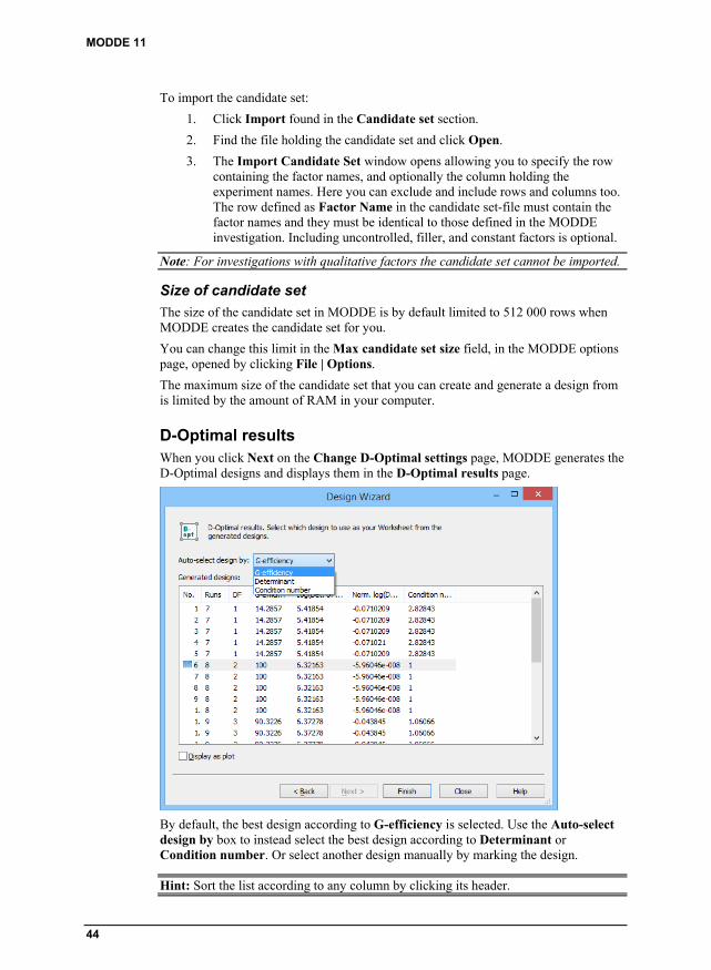
MODDE 11

44

To import the candidate set:

1. Click Import found in the Candidate set section.

2. Find the file holding the candidate set and click Open.

3. The Import Candidate Set window opens allowing you to specify the row containing the factor names, and optionally the column holding the experiment names. Here you can exclude and include rows and columns too. The row defined as Factor Name in the candidate set-file must contain the factor names and they must be identical to those defined in the MODDE investigation. Including uncontrolled, filler, and constant factors is optional.

Note: For investigations with qualitative factors the candidate set cannot be imported.

Size of candidate set

The size of the candidate set in MODDE is by default limited to 512 000 rows when MODDE creates the candidate set for you.

You can change this limit in the Max candidate set size field, in the MODDE options page, opened by clicking File | Options.

The maximum size of the candidate set that you can create and generate a design from is limited by the amount of RAM in your computer.

D-Optimal results When you click Next on the Change D-Optimal settings page, MODDE generates the D-Optimal designs and displays them in the D-Optimal results page.

By default, the best design according to G-efficiency is selected. Use the Auto-select design by box to instead select the best design according to Determinant or Condition number. Or select another design manually by marking the design.

Hint: Sort the list according to any column by clicking its header.

03-Design wizard

45

To see the D-Optimal results as a plot, select the Display as plot check box.

The currently selected design is colored according to the legend.

Click Finish to generate the worksheet. Any already existing design and worksheet will be deleted.

To regenerate a D-Optimal design, using one of the calculated ones, on the Design tab, click New design | Select from already generated D-Optimal designs.

D-Optimal onion pages

Generating the design

After selecting an Onion design, and clicking Next, the Layers page is displayed. This page is organized by layer – from inner (first layer) to outer (last layer).

MODDE 11

46

The following is listed:

1. The number of the Layer (starting from inside).

2. The number of Candidate Runs in the layer for imported candidate sets.

3. The span of the layer defined by its % From (Percentile) and % To distance to the center of the multivariate space. You can change the span of a layer as long as the number of runs in the candidate set remains one and half times larger than the number of design runs in that layer. Overlapping span between layers is not allowed. When you change the span of the layers, MODDE updates the number of candidate set runs in each layer. If the span of the layers overlap, or the number of runs in the candidate set is not large enough, the layer is colored in red and a message indicating the problem is displayed. You must fix the problem before clicking Next.

4. The number of Design Runs in each layer. You can change the number of design runs. The number of desired runs must be at least equal to the number of terms in the model. The recommended number of runs includes 3 degrees of freedom for the outer layer and 1 degree of freedom for the rest of the layers.

5. Select the number of D-Optimal designs, in each layer, you want to generate with the same number of runs. The default number for Repetition is 1.

6. The Model for each layer. You can change the model in each layer. Click the model you want to change and select another model or mark the layer and click Edit model to customize the model. After editing a model, MODDE writes Model edited in the Comment column. MODDE updates the design runs according to the new selected model; default Linear for the inner layers and Interaction for the outer layer.

When you click Finish, MODDE generates several D-Optimal designs in each layer varying the number of runs by plus and minus 2, and displays the Onion D-Optimal results page.

The table on this page displays, for every layer, the generated designs statistics. By default, in this table, the designs with the highest G-efficiency are selected.

You can select a different design in a given layer by marking it in the list or using the Auto-select design by box and selecting a different criterion.

03-Design wizard

47

Onion on the Design tab

Generate

With Onion D-Optimal designs, you cannot generate a new set of D-Optimal designs by clicking New design in the D-Optimal group on the Design tab.

If you want to generate a new set of Onion D-Optimal designs, click Design | Objective. The worksheet will be deleted and you can follow the wizard to generate a new design and worksheet.

Candidate set

To display the candidate set, on the Design tab click Candidate set.

The columns in the spreadsheet are as follows when the candidate set was imported:

1. Design Run number. Corresponds with the experiment number in the worksheet.

2. The Exp Name (experiment name) when available.

3. The Layer number (the innermost layer = 1).

4. The distance to the center of the multivariate space in Percent.

5. The design variables.

When the candidate set is generated by MODDE the additional columns Layer and Percent are unavailable. The layer belonging is displayed in the onion plots.

Reduced combinatorial

Design generation options The Design generation criteria section concerns the criteria on which the design is built while the Design alternatives section controls the number of designs generated what to balance on.

Design runs

Design runs is the number of runs the algorithm will generate, not including the center points. You can change this number as desired. The smallest number of runs accepted is the number of terms currently included in the model.

Replicated runs

The number of runs that should be replicated. The replicated runs are used to get an estimation of the replicate error when lacking center points.

MODDE 11

48

Model terms

The number of terms currently in the model is listed after Model terms. This number is updated after changes in Edit model.

Editing the model

Click the Edit model button to edit the model. The edit model dialog opens and you can edit the model by adding or deleting terms in the specified model. This modifies the number of model terms.

Degrees of freedom

Number of Degrees of freedom of the residuals is calculated as:

Number of design runs – Model terms +1 (when you have center points)

The number of degrees of freedom recommended for D-Optimal and reduced combinatorial designs in MODDE is at least five.

Design runs span

The performance of the design depends on the selected number of runs, N, and the number of terms in the model, p.

MODDE can generate several designs, varying the specified number of runs N and then evaluate them (G-efficiency, Condition number, Determinant) as functions of N.

In the Design runs span box, you can select the number of designs to generate with varying N.

If, for example, you select N 3, MODDE generate 7 designs ranging from N - 3 to N + 3. The default is to generate 5 designs with N 2.

Balancing the design

When you have more than one qualitative or multilevel factor, can select for the design to have the same number of runs at each level of one of the qualitative/multilevel factors. Thus, the design would be Balanced with respect to the qualitative or multilevel factor.

If you want to balance the design on another factor than the default, select the desired factor in the Balance on box.

To be able to get a balanced design, the selected number of design runs must be a multiple of the number of levels of the qualitative/multilevel factor. The number of design runs may be updated, if necessary, to be a multiple of the number of levels of the factor.

Reduced combinatorial design selection page When you click Next on the Change reduced combinatorial settings page, MODDE generates the designs and displays them allowing you to select which design to go ahead and generate.

03-Design wizard

49

By default, the best design according to G-efficiency is selected. Use the Auto-select design by box to instead select the best design according to Determinant or Condition number. Or select another design manually by marking the design.

Hint: Sort the list according to any column by clicking its header.

To see the results as a plot, select the Display as plot check box, see the D-Optimal results subsection earlier in this chapter.

Click Finish to generate the worksheet. Any already existing design and worksheet will be deleted.

51

04-File

Introduction The File tab includes functions that deal with your entire MODDE investigation as opposed to the data itself. Here you can save, print, and send your investigation as well as change settings and options.

The functions available are grouped into 10 groups

Info - Provides access to Protect investigation, the report, and displays investigation properties

Protect investigation - Controls access and changes that can be done to this investigation.

Report - Generate a report for this investigation using the default template or any custom template.

New - provides access to options for creating a new design or importing an existing design.

Experimental design - Start the classical experimental design setup from here.

Import external design - Import a design saved in another file format.

Complement design - Add new experiments to resolve interactions or non-linearities in the current design.

Stability design - Create a design that spans over time to investigate the stability of the product.

Design from candidate set - Import a candidate set and create a design from a D-Optimal selection.

Design from scores - Import scores (factors) from a SIMCA usp file and create a design from a D-Optimal selection.

RED-MUP - Special designs created for 96, 384, or 1536 well plates.

Open - Open an existing investigation.

Save - Save the current investigation.

Save as - Save the current investigation with a new name and/or at a new location.

Print - Print the active window.

MODDE 11

52

Send - Send a copy of the investigation by email as an attachment.

Close - Close the current investigation.

Help - Get help with using and activating MODDE.

Activate MODDE - Activate MODDE over the internet and other options.

View help - Get help using MODDE.

MKS Umetrics on the web - Open MKS Umetrics' website in a browser.

Knowledge base - Open MKS Umetrics' website in a browser, with the Knowledge base page active.

About us

Options - Change options and customize MODDE.

Info The Info section on the File tab provides access to two main features, Protect investigation and Report as well as giving a quick summary of the investigation Properties and displaying the path to the current investigation.

Properties

Under Properties information about the current investigation is listed;

Size

Creation date

Modified date

Objective

Process model

Mixture model

Design

Runs in design

Center points

Replicates

Factors

Responses

Number of runs.

Protect investigation To protect an investigation, you can either lock it so that changes cannot be made, or encrypt it with a password.

04-File

53

Encrypt investigation

Enter a password and the investigation is encrypted and password protected. This investigation can now be opened only with the selected password.

To protect your investigation,

1. On the File tab, click Info,

2. Click Protect investigation,

3. Click Encrypt,

4. In the Encrypt Investigation dialog box, enter a password to use for the encryption and confirm it,

5. Click OK.

Remove encryption

If the investigation is already encrypted, the encrypt option is replaced by Remove encryption.

To remove the encryption,

1. On the File tab, click Info,

2. Click Protect investigation,

3. Click Remove encryption,

4. Enter the password and click OK.

MODDE 11

54

Lock investigation

Locked investigations are automatically fitted when opened. Any plot or list can be displayed, but changes cannot be made to the investigation. The investigation becomes 'Read only' with the exception of the prediction spreadsheet. If you click Permanently, unlock on Save As, a copy of the investigation can be unlocked by clicking Save as on the File tab. When Permanently is selected the investigation cannot be unlocked.

It is possible to also encrypt and password protect the investigation by selecting the Encrypt / Password Protect investigation check box. The investigation is then encrypted. This check box is optional; select it only if you want the investigation to be password protected.

Note: The lock cannot be removed.

Report MODDE has an automatic report generator. To create a new report, on the File tab, click Info, then click Report.

You can also right-click a plot or list and then click Add to report. To add the currently active plot or list to the report, click Add to report on the Tools tab or press Ctrl+R.

Note: When a report was saved with the investigation, MODDE automatically opens that report.

04-File

55

The report can use the MODDE default template or any template previously saved. All formatting functionality is available for writing the text. Plots and lists can be added to the report at any time, as placeholders or actual plots and lists.

A placeholder tells MODDE the desired item to fill from the current investigation when you click Update report on the Home tab of the Report. If you add plots and lists as placeholders and save the template, you can generate a report in the desired format, for any investigation, by selecting the saved template and clicking Update report.

For details, see Chapter 14, Report.

New To create a new investigation on the File tab, click New.

This provides access to options for creating a new design or importing an existing design.

Experimental design On the File tab, click New, then click Experimental design.

Start the classical experimental design setup from here. A wizard will guide you through all steps for setting up an experimental design - traditional designs as well as super saturated and D-Optimal designs. The wizard will always make a design recommendation.

Design wizard

The Design wizard opens when you start a new experimental design. This wizard guides you from the start of the investigation to the generation of the worksheet. The Design wizard can also be opened on the Home tab, in the Quick start group, click Design wizard. Exit the wizard at any time by clicking Finish.

Using existing design To create a new investigation from an existing design, on the File tab, click New, then click either Import external design or Complement design.

Import external design

Import a design saved in another file format.

MODDE 11

56

External data can easily be imported to MODDE for analysis and optimization, as follows:

1. Click File | New.

2. Click Import external design.

3. Browse and select the file to import.

4. Click Next and specify what is what in the Data Specification dialog.

Complement design

The current investigation can be complemented with new experiments to resolve interactions or non-linearities.

To add new experiments to the current design, on the File tab, click New, then click Complement design.

A wizard will guide you through classical fold over complementation or specific requests.

Use Complement design when you want to:

Estimate separately a set of terms (interactions, or main terms and interactions) that were confounded in a Resolution III or IV fractional factorial design.

Complement a screening design to an RSM design supporting the full quadratic model.

Complement a screening design to estimate selected curvature effects.

Add additional experimental runs to improve the quality (i.e. the condition number or G-efficiency) of an existing set of experiments.

Use already performed experiments in a Doehlert design to set up a new Doehlert; moving the center of the design or adding a factor.

Use already performed experiments in a Super-Saturated Plackett Burman design to add experiments resulting in a regular Plackett Burman design.

Available complementing methods

You can complement your design using the following complementing methods:

Fold over: With screening fractional factorial designs of resolution III and N (number of runs) equal to 8 or 16, it is usually recommended to complement by fold over. For more, see the Fold over subsection later in this chapter.

Estimate squares of selected factors in factorial designs: If the screening design indicates the presence of curvature, you may want to estimate the square terms in selected factors or you may want to upgrade your design to a full RSM in these selected factors. For more, see the Estimate squares terms subsection later in this chapter.

D-Optimal: This option should only be selected if it is not possible to use a different complementing method. If you want to upgrade the design to support a customized model, or if your investigation contains mixture factors, select D-Optimal. For more, see the Complementing a design with D-Optimal subsection later in this chapter.

04-File

57

Design specific complementing methods

Doehlert: When you have performed a Doehlert design and want to move the design center or add a factor. For more see the Complementing Doehlert designs subsection later in this chapter.

Screening to RSM Rechtschaffner: When you have performed a screening Rechtschaffner design. Complemented by adding the star points resulting in a 3-level Rechtschaffner.

Plackett Burman Super-Saturated to Plackett Burman: When you have performed a PBSS. Complemented with runs adding up to a regular Plackett Burman design.

Fold over

When you choose to complement your design with fold over MODDE makes a new investigation consisting of the design of the current investigation plus its fold over (complement). The fold over design has as many experimental runs as the original design.

Fold over designs are available for fractional factorial design of resolution III or IV and Plackett Burman designs.

With the complete design (original + fold over), all main effects are clear from 2 factors interactions. With resolution III and IV designs MODDE automatically adds a block factor. You may remove the block factor from the model in Edit model.

To fold over your design:

1. Click File | New | Complement design.

2. Click Fold over and then click Next.

3. Enter the name and location of the new investigation. It is recommended to add an additional center point to detect a shift in the mean.

4. Click Finish and the new investigation opens.

Estimate squares terms in a screening design

For this complementing method to work well the original design should be of resolution V or the collapsed design in the selected factors has to be a full factorial.

On the File tab, click New, and then click Complement design:

1. Click Estimate square terms in a screening design and click Next.

2. Select the factors for which to estimate the square terms. Note that the calculated star distances for CCC and CCO are displayed.

3. Optionally change the star distance. If the star distance is not changed, the design is complemented to a CCF design by adding the face center runs. To change, click the desired star distance to automatically enter it in the Star distance field. Click Next.

4. Enter the name, location of the new investigation and number of additional center points.

5. The model has been updated with the squares of the selected factors. The unselected factors are set on their averages in the worksheet.

MODDE 11

58

Complement Doehlert

Doehlert designs can be complemented by expanding the design region or adding a factor.

To complement a Doehlert design, click Doehlert in the Complement Design Wizard and click Next.

04-File

59

As the dialog suggests you can complement by:

Leaving the default Select new center selected and selecting one of the experiments of the design as the center of a new Doehlert design.

Selecting Add factor and typing the name of the new factor and typing the Center and Range in the respective boxes. The value you type in Center is the value that will be entered in the design for the already performed experiments, for the new factor.

Select how to complement, click Next, enter the name, location of the new investigation and number of additional center points, and then click Finish to generate the new investigation.

D-Optimal

Complementing a design D-optimally is the most flexible way of complementing a design.

Process factors only

On the File tab, click New, and then click Complement design:

1. With D-Optimal marked, click Next.

2. Click Edit model... to open the Edit Model dialog box and add model terms. Click OK to return to the Complement Design Wizard.

3. MODDE recommends the number of additional new design runs based on the specified model, to ensure the proper degrees of freedom.

4. Click Next.

5. Enter the name and location of the new investigation and click Finish. The D-Optimal pages in the Design wizard guide you in generating the new investigation. Here the original design runs in the selected factors are used as inclusions and the displayed Design runs in the D-Optimal page includes the inclusions. The additional new runs are selected D-optimally to support the selected model.

MODDE 11

60

Mixture factors

Complementing the design D-optimally with mixture factors, only allows changing the model in Settings | Model available after entering the name and location of the new investigation.

The displayed number of runs includes the original design runs. Click Next, the wizard guides you in generating the new investigation.

Mixture and process factors

Complementing a design D-optimally with mixture and process factors, only allows changing the model in Settings | Model available after entering the name and location of the new investigation. The objective is set to Split objective.

The displayed number of runs includes the original design runs as inclusions. Click Next and the wizard guides you in generating the new investigation.

Specific application design MODDE provides options to create specific application designs such as Stability design, Design from candidate set, Design from scores, and RED-MUP.

To create a specific application design, on the File tab, click New, then click the desired option.

Stability design

In stability testing Combinatorial designs are used to evaluate all combinations of factors and settings over time. The purpose is to ensure that none of the quality attributes for the stability testing will exceed the specification during the products specified shelf life.

04-File

61

In a typical stability test all combinations are tested over several time points (i.e. 0, 3, 6, 9, 12,… months). A way to reduce the total number of tests is to distribute subsets of all possible combinations to specific time points stipulating that all combinations are tested over a specified period of time. This design strategy is called Complementary combinatorial design.

For example, 3 factors (n) with 2+3+4 levels = 24 possible combinations/experiments can be distributed over 2 time points as 12+12 experiments or over 3 time points as 8+8+8 experiments.

The number of possible combinations k can be divided into p subsets, k/p, where p is an integer. Each subset mi will contain a unique set of combinations. One constraint is that each subset mi shall be as balanced as possible and the best possible representation of k.

For more information of the practical handling in MODDE, see the Stability design appendix.

Algorithm short version;

1. Choose an n-dimensional design region with k runs in its candidate set and a design with m runs: m = k/p.

2. Decompose factors into p sets.

3. Generate the matrix M = 2 - (p, n, pn-3) OA (orthogonal array) from Latin Squares.

4. Reduce M to all rows mapping to non-empty sets.

5. Map each row of M to the decomposed factor sets and make a full factorization of the elements in the active sets: Mi.

6. The final design D is given by concatenating the mappings Mi from step 5.

Design from candidate set

Import a candidate set and create a designed selection of observations. The selection can be done using layers (Onion) or D-optimally.

To create a design based on a candidate set, on the File tab, click New, then click Design from candidate set.

Onion design in regular factors with imported candidate set

When you want create an onion design from an imported candidate set other than scores from SIMCA:

1. On the File tab, click New, then click Design from candidate set.

2. Click Browse to find the file holding the candidate set. Many file types are supported.

3. Click Next to open the Import candidate set dialog box specifying factor names, experiment names, and data.

4. Click OK to open the factors page of the Design wizard. When the candidate set has been imported in this way you cannot modify or add factors using the Design wizard.

MODDE 11

62

5. To place constraints on the factors, click the Place constraints on the experimental region check box and click Next to open the constraints page of the Design wizard.

Note: Only regular factors are imported here. If your candidate set contains qualitative or formulation factors you have to enter the factors and settings in the Factor Definition dialog box and import the candidate set from the D-Optimal page instead.

The designs available here are Onion and D-Optimal designs. Onion is only available when there are enough experiments in comparison with the number of factors.

Design from scores

This is a typical QSAR application where a subset of molecules is selected by design. Molecules described by many variables are compressed to score vectors in SIMCA. These score vectors can then be imported directly from the SIMCA usp file.

To create a design based on imported scores from a SIMCA file, on the File tab, click New, then click Design from scores.

Multivariate designs

To be able to import scores from a SIMCA project, SIMCA-P 10 or later needs to be installed. The only designs available are D-Optimal and Onion.

When you want to create a design using the scores from a SIMCA project as factors:

1. On the File tab, click New, then click Design from scores.

2. Click Browse to select the SIMCA project.

3. Select the model from the Model box and click Next to import the factors (scores) from SIMCA. The score variables with all observations (rows) are then automatically loaded from the SIMCA file and define the candidate set.

4. Click Next to continue through the design wizard and the creation of the D-Optimal or onion design.

Note: SIMCA opens automatically and remains open in the background while focus returns to MODDE.

RED-MUP

Rectangular experimental design for multi unit platforms - an efficient and time-saving approach for application of DOE to 96, 384 and 1536 well plates.

RED-MUPs are designs available for 96 (8x12), 384 (16x24), and 1536 (32x48) runs. The designs are built from sub-designs.

04-File

63

To create a RED-MUP:

1. On the File tab, click New, then click RED-MUP.

2. Define all factors for the two sub-designs and then click Next.

3. Define the responses and then click Next.

4. Select the objective for both the vertical and the horizontal designs: Screening or Optimization (RSM).

5. Leave the factors that should be included in the vertical design with fewer runs to the left.

6. Move the factors that should be included in the horizontal design to the right.

7. On this page you can also select the number of plates used, and if applicable the plate factors that contain plate information.

8. Select the desired plate size in the Plate size box and optionally select the Plate/Block factor interactions check box.

9. Click Next to select the vertical design then click Next again to select the horizontal design. MODDE adds center points when the selected design does not fill up the plate size.

Note: Some special RED-MUP designs, that aim to make better use of the plate, are available for the 96 well plates (8 x 12).

Open To open a MODDE investigation, on the File tab, click Open.

You can also open an existing investigation by clicking Open on the Quick Access Toolbar or using the Windows keyboard shortcut Ctrl+O.

MODDE 11

64

Recent investigations The Recent investigations list shows recently opened investigations.

Click the pin icon to the right of the investigation name to pin the investigation to the top of the list. Click the name of the investigation in the list to open any recent investigation.

Recent folders The Recent folders list shows folders where you have recently opened or saved an investigation.

Click the pin icon to the right of the folder's name to pin a folder to the top of the Recent folders list. Click the folder name in the list to open any recently opened folder.

Browse To browse for existing MODDE investigations, click Browse.

Save To save the current investigation, on the File tab, click Save. You can also use the

Windows keyboard shortcut Ctrl+S or click the save icon on the Quick Access Toolbar at the top of the MODDE window.

Save as To save the current investigation in a different location or with a different name, click Save as on the File tab, then click one of the folders in the Recent folders list or Browse. In the Save As dialog box that opens, enter the new name and location of your investigation. MODDE switches to the "new" investigation.

Save plot as An individual plot can be saved in a variety of formats.

To save a plot, right-click the plot, then click Save as....

This opens the Save Plot dialog box.

04-File

65

For details about the Save Plot dialog, see the Save or Copy a plot section later in this chapter.

Save list as To save a list,

1. Right-click the list.

2. Click Save as....

3. Select location, file name, and file type.

4. Click Save.

Lists can be saved as either webpages (htm/html) or as text files (txt).

Save or Copy a plot The Save Plot and Copy to Clipboard dialog boxes are very similar, merely the presence/absence of the Format drop down differentiates them. When copying, the plot format can be selected in this dialog box while, for save, it can be selected in the Save As dialog which opens after clicking OK.

Note: For plots with constants, the constants are copied, saved and printed if the property pane is visible.

MODDE 11

66

Size

The size of the plot is defined by the values in the Width and Height fields. These fields are automatically updated when switching between the predefined sizes in the Size box. Likewise, the content of the Size box is updated when changing the width and height.

Note: To keep the aspect ratio of the plot while customizing the size, select the Lock aspect ratio check box before changing.

The available options in the Size drop down box are,

Original size - the current plot size

Suitable for documentation

600 x 375 Standard size

300 x 300 Square, fits two side by side

600 x 600 Square

Suitable for presentations

755 x 465 Fits one plot per slide

755 x 270 Fits two above and below

370 x 465 Fits two side by side

Custom sizes

Add custom size - opens the Add Custom Size dialog box with the current plot size predefined. Clicking OK adds the specified size under the Custom sizes header.

Delete customizations - restores the list to its original content.

Edit and delete

To edit the current size, click the Edit current size pencil to the right of the Size drop down.

To delete the current size, click the Delete current size garbage bin.

Size preview

Selecting the Size preview check box displays the plot exactly as it will be saved or copied. This feature allows you to verify that the layout and text formats harmonize with the selected save/copy size before inserting/pasting it.

Print quality and plot format

The default print quality is 96 dpi. This is sufficient for the web and presentations, but not for high quality print where 300 dpi is recommended.

The plot formats available are Bitmap (BMP), EMF (only 2D), PNG, JPG, Encapsulated PostScript (EPS), and SVG (only 3D and only when saving).

Note: Using EPS with high dpi creates a very large plot file.

04-File

67

Restore to original list of sizes

After making changes to the Size list by adding custom sizes or deleting original sizes the list can be restored to its original content by, at the bottom of the Size list, clicking Delete customizations.

Print To print, preview or change the print setup click File | Print.

When a list is the active window, the Print in color check box is available here. To print your list without background coloring (whether in color or in gray scale), clear this check box.

For plots with constants, such as the Contour plot, the constants are copied, saved and printed if the property pane is visible.

Note: Plots are printed as viewed on the screen except when printing to a pdf writer.

Print is available for the active plot or list. MODDE provides a variety of ways to print,

Ctrl+P, the Windows keyboard shortcut for print,

Right-click the desired plot or list and click Print,

On the File tab, click Print.

Send

Send as attachment On the File tab, click Send, then click Send as attachment to send a copy of the investigation by email as an attachment.

MODDE 11

68

Close On the File tab, click Close to close the currently open investigation.

Options On the File tab, click Options to access the options for a number of sections of MODDE.

The Options dialog box comprises all general options as well as investigation specific options and other customizations, such as Theme (not described further here).

MODDE options The MODDE options page is divided into the parts Audit trail, General, and Plot.

Audit trail

Set Audit trail options.

Enable the audit trail for new investigations - Automatically enables the audit trail for all new investigations.

For more, see the Audit trail section in Chapter 10, View.

04-File

69

General

Under General you can change the following options,

Automatically display output window - Automatically open or activate the output window when MODDE encounters warnings and errors. This window displays details about the warnings and errors.

Automatic fit - Automatically fit the investigation when it is opened.

Close open investigation when opening a new investigation - Close already open investigation when opening or creating a new investigation.

Factor axes in back transformed units - Display factors on plot axes in back transformed units.

Max number of layers in onion designs - Maximum number of possible layers for an Onion design. MODDE's default is 10.

Max candidate set size - The maximum number of rows in the candidate set. This number will prevent MODDE from creating candidate sets that are too large. The maximum size of the candidate set that you can create and generate a design from is limited by the amount of RAM in your computer.

Replicate tolerance - The replicate tolerance [0 .. 0.20] is the number used when MODDE decides whether experiments can be considered to be replicates or not. Default is 0.1, that is, 10% of half the range for each factor.

Save Design Space Explorer calculations - Include the Design Space Explorer calculated results with investigation (.mip) when saving it. If the calculations are saved with the investigation, no recalculations are necessary when redisplaying this plot. WARNING! When selected, the .mip may become large.

Show expanded design factors in RED-MUP worksheet - Show each design factor expanded.

Show units in lists - Show units after the factor and response names in lists and spreadsheets.

Plot

Header format - Select which of the two header formats to use. Leaving Default results in 'Header format 1' for investigations with short names and 'Header format 2' for investigations with long names.

Header format 1 - When selected, header format 1 by default displays plot type, investigation name and fit method on the first row and coloring and label information on the second.

Header format 2 - When selected, header format 2 by default displays plot type and fit method on the first row, investigation name on the second and coloring and label information on the third.

Plot engine - Select which plot engine to use for 2D plots. Available options are Direct2D or GDI+. 3D plots are always displayed using GDI+.

Note: The order and what is displayed in the headers can be changed as desired using the displayed terminology. Maximum number of header rows is four.

MODDE 11

70

Investigation options On the File tab, click Options, then click Investigation options to view the settings valid for the current investigation, grouped under the headers Audit trail, General, Statistical options, and Design space and optimizer options.

Available settings include,

Audit trail

When Enable the audit trail is Yes, the Audit Trail logs every change that affects the investigation. Your administrator may have locked the settings on this tab. By default the audit trail is disabled. For details, see the Audit trail section in Chapter 10, View.

General

Design matrix

Select the data to display in the design matrix. Available options are The design as generated by MODDE and Current Worksheet scaled and centered (default).

Factor representation

Select whether to show the Factor name (default) or the Factor abbreviation in lists and spreadsheets.

Factor presentation [Qualitative]

Select whether to display the qualitative factors in the Regular (default) format, showing the orthogonal settings, or Extended, showing all settings. This option is valid for all plots and lists displaying factors except the coefficient plot.

04-File

71

Factor presentation [Qualitative, Coefficient plot]

Select whether to display the qualitative factors in the Regular format, showing the orthogonal settings, or Extended (default), showing all settings. This option is valid for the coefficient plot only.

Number format

Select the number of decimals to display in lists and tables. Available

options are Auto (default), .00, .000, .0000, .00000, and Scientific (e.g. 1.234e-10).

When exporting unscaled coefficients to use in other applications, use the scientific format to get maximum precision in the coefficients.

Plot label type

Select None, Experiment number (default), Experiment name, Run order, or Combination ID (available for stability designs only).

For stability designs the default Experiment name is the Combination ID and the Time, e.g. C1:T0 for the first row. The Combination ID denotes a specific combination of settings for all factors but the Time factor.

Response representation

Select whether to show the Response name (default) or the Response abbreviation in lists and spreadsheets.

Statistical options

Alpha level

Select the Alpha level for the lack of fit plot. Available options are 1%, 5% (default), and 10%.

Coefficients

Select the type of coefficients. Available options are Scaled and centered (default for the regular coefficient plot), Unscaled, PLS orthogonal, and Normalized (default for the coefficient overview plot).

To select presentation format for qualitative factors in the Coefficient plots, use the Factor presentation [Qualitative, Coefficient plot] option earlier in this page. By default the factors are displayed in the Extended form in this plot, showing all settings.

For more, see the Coefficients subsection later in this section and the Coefficients section in the Statistical appendix.

Interval type and probability levels

Select the type of interval to use to estimate the uncertainties. Available interval types are Confidence (aka Average), Prediction (aka Individual), and Tolerance.

An interval estimation is used in statistics as an uncertainty measure of a population parameter computed from sample data.

The simulation will generate points with variance based on the selected interval estimate. This will in turn generate the required safety margins that correspond to the defined probability limit of the ideal average prediction. The safety margin increases from Confidence to Prediction (and in general) to Tolerance.

We use interval estimates for two purposes in MODDE:

to assess if model parameters are significantly different from zero (null-hypothesis significance tests) and

MODDE 11

72

to state an interval within which we are confident that we find future predictions.

For more, see the Interval type and probability levels subsection later this section and the Interval estimates subsection in the Statistical appendix.

Prediction block effect

Select to use fixed or random block effect in predictive functions.

Select the block factor as Fixed effect when the external variability can be set at will and the primary objective for blocking is to eliminate that source of variability.

Select the block factor as Random effect when the external variability cannot be controlled and set at will, and the primary objective is to make prediction without specifying the block level, and taking into account the external variability.

For more, see the Random versus fixed block factor section in the Statistical appendix.

R2

Select the type of R2 to display in the summary plots. Available options are R2 [explained variation] (default) and R2 adjusted [explained variance].

Residuals

Select the type of residuals to display in the residual plots. Available options are Raw in the original units, Standardized, and Deleted studentized. The default depends on fit method and number of degrees of freedom. For more, see the Residuals section in the Statistical appendix.

Design space and optimizer options

DPMO limit

Enter the default DPMO limit for the investigation. DPMO = Defects Per Million Opportunities.

This default DPMO limit is used in all Design space plots and Setpoint features. The default value is 10 000, which corresponds to 1% outside.

Interval type and probability levels

Select the type of interval to use to estimate the uncertainties. Available interval types are Confidence (aka Average), Prediction (aka Individual), and Tolerance.

An interval estimation is used in statistics as an uncertainty measure of a population parameter computed from sample data.

The simulation will generate points with variance based on the selected interval estimate. This will in turn generate the required safety margins that correspond to the defined probability limit of the ideal average prediction. The safety margin increases from Confidence to Prediction (and in general) to Tolerance.

We use interval estimates for two purposes in MODDE:

to assess if model parameters are significantly different from zero (null-hypothesis significance tests) and

to state an interval within which we are confident that we find future predictions.

For more, see the Interval type and probability levels subsection later this section and the Interval estimates subsection in the Statistical appendix.

04-File

73

Audit trail When the Audit Trail is turned on each investigation in MODDE has a separate audit trail. Each audit trail consists of one or more sessions that in turn consist of events. A new session is started and appended to the audit trail when an investigation is opened, and ends when the investigation is saved.

In addition to logging events, MODDE logs information about the user, and date and time of the events.

To view the audit trail, click the Audit Trail tab in the Output / Notes / Audit trail pane. If this tab is not shown, display it by selecting the Audit Trail check box on the View tab.

Enable and disable the Audit Trail

By default the audit trail is disabled.

To turn it on for the current investigation, in File | Options, on the Investigation options page, under Audit trail, select Yes in Enable the audit trail.

To turn on the audit trail for new investigations, in File | Options, on the MODDE options page, under Audit trail, select Yes in Enable the audit trail for new investigations.

Administrators can disable the turning on and off of the audit trail, i.e., always have it on or off. For instructions on how to disable the audit trail options, see the knowledge base at www.umetrics.com.

Save or clear the Audit Trail

To empty the audit trail, in the Audit Trail pane, right-click and click Clear Audit Trail.

To save the current version of the audit trail, separate from the investigation, in XML format, in the Audit Trail pane, right-click and click Save as.

Audit trail and internet explorer

MODDE uses Internet Explorer functionality to display the audit trail.

Logged in the audit trail

Specific actions the MODDE audit trail logs are:

Factors (adding, modifying, deleting), displaying all details about the factor after the change

Responses (adding, modifying, deleting), displaying all details about the response after the change

Constraints (modifying, deleting)

Candidate set

Inclusions

Reference mixture

Objective

Generators

Design

MODDE 11

74

Complement design

Model

Worksheet, every change of every cell

Fit method

Activation and deactivation of the Audit Trail.

The audit trail also registers when a digital signature in the Audit trail is incorrect.

Coefficients

Scaled and centered coefficients The regression coefficients that are displayed in MODDE are computed for centered and scaled data. It is also possible to select to display "unscaled and uncentered" coefficients.

The scaled and centered coefficients are the coefficients of the fitted model, for which the factors were centered and scaled. The default scaling in MLR is orthogonal scaling. With PLS, the factors are centered and scaled to unit variance.

Orthogonal coefficients in PLS The "centered and scaled" coefficients in PLS regression models are computed from factor values scaled to unit variance.

The orthogonal coefficients in PLS regression re-express the coefficients such that they correspond to factors that are centered and orthogonally scaled, i.e., by using the mid-range and low and high values in the factor definition (coded as -1 and 1), see the Scaling subsection for more details. Orthogonal coefficients in PLS regression models are not available when there are only formulation factors in the investigation.

With process and mixture factors, the PLS orthogonal coefficients refer to process factors scaled orthogonally, and mixture factors unscaled (original units).

The orthogonal coefficients in PLS regression models are only available when the model is fit with PLS regression.

Note: The orthogonal coefficients in PLS regression models are only meant for comparison with the corresponding MLR coefficients. They are incorrect unless the design is balanced and the mean is equal to the mid-range.

Unscaled The unscaled coefficients are the coefficients corresponding to unscaled, uncentered data. When exporting unscaled coefficients to use in other applications, be sure to use the E-format in order to obtain maximum precision in the coefficients.

Normalized coefficients To make the coefficients comparable between responses when the responses have different ranges, the "centered and scaled" coefficients are normalized with respect to the variation in Y. That is, they are divided by the standard deviation of their respective response, i.e., by the standard deviation in the corresponding Yi, for i = 1,2,…,m.

04-File

75

Confidence interval Intervals for coefficients (such as e.g., a confidence interval) and predictions are computed using the total number of observations, regardless of missing values when the regression model is a PLS regression model and all polynomial models (i.e., the polynomial model specified by the factors) for all responses are the same. For MLR and PLS regression models with different polynomial models for different responses, the total number of observations is the number of elements in the response without missing values. This total number of observations is displayed as N at the bottom of plots and lists.

Extended or compact format For qualitative factors at q levels, with q > 2, MODDE generates q - 1 dummy variables, indexed from 2 to q.

By default the Coefficient plot displays all q settings using the Extended format. See the Investigation options subsection in Chapter 4, File, for details.

Interval type and probability levels

Select the type of interval to use to estimate the uncertainties. Available interval types are Confidence (aka Average), Prediction (aka Individual), and Tolerance.

An interval estimation is used in statistics as an uncertainty measure of a population parameter computed from sample data.

The simulation will generate points with variance based on the selected interval estimate. This will in turn generate the required safety margins that correspond to the defined probability limit of the ideal average prediction. The safety margin increases from Confidence to Prediction (and in general) to Tolerance.

We use interval estimates for two purposes in MODDE:

to assess if model parameters are significantly different from zero (null-hypothesis significance tests) and

to state an interval within which we are confident that we find future predictions.

There are several types of interval estimates that can be used in MODDE. A common statement is to say that with a confidence of e.g. 95 % we will find a future sample in this region enclosed by the interval, i.e. average ± interval.

The types of intervals available in MODDE are;

Confidence interval

This interval encloses average of the true population, with some confidence, and is mainly used to illustrate the variance of the model coefficients.

Prediction interval

This interval encloses a region within which we are confident that the next observation will fall.

Tolerance interval

This interval encloses a region within which we are confident that some proportion of future samples will fall.

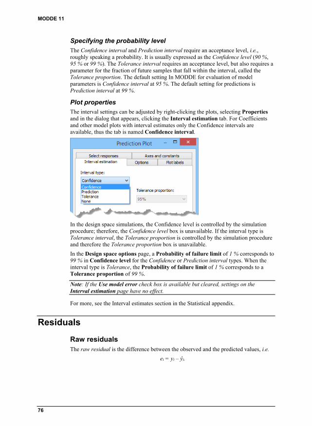
MODDE 11

76

Specifying the probability level

The Confidence interval and Prediction interval require an acceptance level, i.e., roughly speaking a probability. It is usually expressed as the Confidence level (90 %, 95 % or 99 %). The Tolerance interval requires an acceptance level, but also requires a parameter for the fraction of future samples that fall within the interval, called the Tolerance proportion. The default setting In MODDE for evaluation of model parameters is Confidence interval at 95 %. The default setting for predictions is Prediction interval at 99 %.

Plot properties

The interval settings can be adjusted by right-clicking the plots, selecting Properties and in the dialog that appears, clicking the Interval estimation tab. For Coefficients and other model plots with interval estimates only the Confidence intervals are available, thus the tab is named Confidence interval.

In the design space simulations, the Confidence level is controlled by the simulation procedure; therefore, the Confidence level box is unavailable. If the interval type is Tolerance interval, the Tolerance proportion is controlled by the simulation procedure and therefore the Tolerance proportion box is unavailable.

In the Design space options page, a Probability of failure limit of 1 % corresponds to 99 % in Confidence level for the Confidence or Prediction interval types. When the interval type is Tolerance, the Probability of failure limit of 1 % corresponds to a Tolerance proportion of 99 %.

Note: If the Use model error check box is available but cleared, settings on the Interval estimation page have no effect.

For more, see the Interval estimates section in the Statistical appendix.

Residuals

Raw residuals The raw residual is the difference between the observed and the predicted values, i.e.

ei = yi – ŷi.

04-File

77

Standardized residuals The standardized residual is the raw residual divided by the residual standard deviation

estd,i = ei / s,

where s is the residual standard deviation.

Residual plots for PLS regression present standardized residuals by default.

Deleted studentized residuals MODDE defaults to plotting Deleted studentized residuals when fitting with MLR and the model has at least three (3) real degrees of freedom. Deleted studentized residuals are not available when fitting with PLS regression.

The Deleted studentized residual is the raw residual (ei) divided by an estimate of its standard deviation. The estimation of the standard deviation is computed from the “deleted” standard deviation (si), which is the residual standard deviation (si) computed with observation i left out. When the ith residual is excluded like this, the residual is sometimes said to be externally studentized. The variance of the ith residual is defined as

where is the ith element of the hat matrix, sometimes denoted leverage. Thus the standard deviation of the residual is

Hence, the Deleted studentized residual is computed as

where s-i is the estimate of the residual standard deviation with the ith sample left out.

For more information see e.g., Belsley, Kuh and Welsch (1980).

Note: Deleted studentized residual requires at least three degrees of freedom.

References

Belsley, David A.; Kuh, Edwin and Welsch, Roy E. Regression Diagnostics: Identifying Influential Data and Sources of Collinearity. John Wiley and Sons, New York, 1980.

DPMO limit

Enter the default DPMO limit for the investigation. DPMO = Defects Per Million Opportunities.

This default DPMO limit is used in all Design space plots and Setpoint features. The default value is 10 000, which corresponds to 1% outside.

MODDE 11

78

List options

Use this page to change the appearance and properties of lists.

General options such as gridline style and header in bold.

Default colors for text and suspicious value.

Default background color for factors and responses.

Default colors for header background for different types of factors and responses.

Default background colors for different types of data.

Correlation matrix threshold and factor and response background colors.

Customize ribbon On the File tab, click Options, then click Customize ribbon to access the page.

1. Select the command in the left box that you want to place.

2. Click the location in the right box where you would like the command to be shown.

3. Click Add.

4. Click Close to return to MODDE.

04-File

79

Note: With this dialog open, all buttons and tabs currently displayed can be dragged to new positions. Buttons can be removed by pulling them down.

Customize quick access toolbar On the File tab, click Options, then click Quick access toolbar.

1. Select the command in the left box that you want to add.

2. Click Add.

3. Click Close to return to MODDE.

Keyboard shortcuts MODDE includes many keyboard shortcuts in order to access commonly used functions. Many of these shortcuts will be familiar to Windows users, while some are MODDE specific.

Key assignments can be modified as desired in the Options dialog, Keyboard page.

MODDE 11

80

KeyTips

In order to quickly navigate around MODDE using almost exclusively the keyboard instead of the mouse, MODDE implements the same system of KeyTips as Microsoft Office.

1. Press the Alt key to see the KeyTips.

2. Then press the indicated number or letter to run the associated command.

General keyboard shortcuts

Copy: Ctrl+C, Ctrl+Insert

Paste: Ctrl+V, Shift+Insert

Cut: Ctrl+X, Shift+Delete

Print: Ctrl+P

Undo: Ctrl+Z, Alt+Backspace

Save: Ctrl+S

Delete: Delete

Select all: Ctrl+A

Insert: Insert

Full screen: F11

Start a new investigation: Ctrl+N

Open a different investigation: Ctrl+O

04-File

81

MODDE specific keyboard shortcuts

Open the Design wizard: Ctrl+W

Open the Analysis wizard: Alt+W

Add to favorites: Ctrl+D

Add to report: Ctrl+R

Properties: Alt+Enter

Restore On the File tab, click Options, then click Restore to restore MKS Umetrics' defaults.

There are three sections, Format plot, Favorites, and Don't show again messages.

Help The Help page on the File tab provides various resources for support using MODDE, handling licenses, and about the program itself.

MODDE 11

82

Activate MODDE

To open options related to activating MODDE,

1. Click the File tab.

2. Click Help.

3. Click Activate MODDE.

Follow the instructions in the dialog boxes.

View help Get help using MODDE. Opens the MODDE Help window. MODDE's help is based on this user guide.

MKS Umetrics on the Web Opens MKS Umetrics' website in a browser.

Knowledge base Opens MKS Umetrics' website in a browser, with the Knowledge base page active.

About us MKS Umetrics is a world leader of Multivariate Technology. We provide software for Design of Experiments and Multivariate Data Analysis. Tools that transform your data into information, guiding you to confident decisions and helping you understand complex products and processes.

We offer complete solutions for off-line as well as on-line applications for continuous and batch processes. All supported by training and consulting services to ensure you get the most of your data.

83

05-Home

Introduction The Home tab collects some of the most used functions together in one place, making them easy to find and access. Some functions are located only on this tab, while most functions are also located on other tabs. When a function is also located elsewhere, this chapter only provides a brief description and directions to the main description in another chapter.

The functions on the Home tab are divided into groups in order to make commonly used functions easier to find,

Quick start group

Design wizard - provides guidance through the process of setting up a new investigation or changing an existing one.

Analysis wizard - provides guidance through the main steps of analyzing a model.

Investigation group

Specification - opens the Specification window with worksheet, factors and responses, and constraints available.

Model group

Edit model - to add and remove model terms, see the Model list.

Fit model - to refit the current model.

Summary of fit - provides access the summary plots and lists.

Diagnostics & interpretation group

Overview - opens the Overview plot window displaying a customizable selection of plots.

Coefficients - provides access to coefficient plots and lists

Residuals - provides access to the residuals lists and plots.

Observed vs. predicted - displays observed values vs. predicted values.

Contour - opens the contour plot wizard.

MODDE 11

84

Sweet spot - creates a plot highlighting values that are within the user specified range.

Design space - opens the Design Space Plot wizard.

Optimize group

Optimizer - opens the optimizer window.

Editing group

Exclude - excludes the currently selected experiment or data point.

Undo - reverses the last action.

Design wizard The Design wizard is a set of pages that guide you through the steps of setting up your investigation. The Design wizard covers factors, constraints, responses, objective, and model.

To access the Design wizard, on the Home tab, in the Quick start group, click Design wizard.

Hint: Press Ctrl+W to open the Design wizard.

For more information, see Chapter 3, Design wizard.

Analysis wizard The Analysis wizard provides guidance through the main steps of analyzing a model and is the recommended method for making changes to and adjusting the model. The Analysis wizard covers:

Reviewing raw data

Fitting data

Diagnostics

Refining the model.

Note: When opening the Analysis wizard, the investigation is fitted using the default fit method.

Accessing the Analysis wizard

On the Home tab, in the Quick start group, click Analysis wizard.

Included graphs and plots

Replicates

Histogram

Summary of Fit

Coefficients

Residuals Normal Probability

05-Home

85

Observed vs. Predicted.

Toolbar functions

The functions available in the Analysis wizard,

Response: Swaps between active responses.

Exclude: Excludes model terms or experiments.

Undo: Reverses the most recent change to the model.

Regression line: Toggles the regression line.

Show limits: Toggles lines for applicable Min, Max, and Target levels.

Transform: Available when looking at the histogram; opens the Transform Response dialog box.

Edit model: Available when looking at the coefficients plot; opens the Edit Model dialog box.

Square test: Available for the coefficients plot, when no square terms are included and the square test detects significant square terms.

Interaction test: Available for the coefficients plot, when there are significant interactions detected and the design is resolution IV.

Replicates Replicates is the first page shown when opening the Analysis wizard. This page provides a quick overview of the raw data.

Understanding the plot

Experiment points above the red Max line or under the Min line are generally undesirable.

MODDE shows replicated experiments as blue (default) points on the same replicate index.

MODDE 11

86

The variation of repeated experiments should be less than the overall variation for the response.

Working with the plot

It is possible to identify outliers when examining the Replicates plot.

Some of the common causes and suggested solutions to outliers are:

Incorrect data entry in the worksheet – In this situation correct the worksheet and refit.

Experiment incorrectly carried out – If the experiment was not done correctly, repeat the failed experiment and refit.

The deviating result is correct and the experiment does not fit the model – Empirical models are only valid within a limited interval. If the deviating point is correct but uninteresting, then remove it from the analysis and refit the model without it. If the deviating point is in an interesting area, it may be necessary to construct a finer-grained design in that area.

Click Next to see the Histogram for the current response.

Histogram Histogram is the second page of the Analysis wizard. This page provides the opportunity to see the shape of the response distribution and apply a transformation if required.

Understanding the plot

A proper estimate of the distribution requires a minimum of 11 observations. The important decision to make at this step in the Analysis wizard is to decide if a transformation is required. By selecting an appropriate transformation, a non normal distribution might be transformed to normal distribution. In general, normally distributed responses will give better model estimates and statistics.

If a response has already been transformed, the response will have a tilde ("~") after it's name in the plot. To see what transformation has been applied, click Transform.

05-Home

87

Transforming the response

If the distribution is not a normal "bell-shaped" distribution, then it is likely a transformation is required.

The desired distribution is a "bell shaped" normal distribution.

If there is a positive skewness, a log transformation is needed.

If there is a negative skewness, a negative log transformation is required.

Hint: Biological systems almost always require a logarithmic transform.

To apply a transform:

1. Determine the required transformation.

2. Click Transform.

3. Click the desired transformation in the Transformation list.

4. Change the values of C1, C2, and C3 (if available) from default values if the data requires it.

5. Click Apply to see the transformed response.

6. Click OK to return to the Analysis wizard.

Click Next to go to Summary of Fit.

Click Back to go to Replicates.

MODDE 11

88

Summary of Fit The Summary of Fit page of the Analysis wizard provides a summary of the basic model statistics.

Understanding the plot

Summary statistics are presented in four parameters (R2, Q2, Model validity, and Reproducibility) where 1, or 100%, is perfect. R2 and Q2, the first two columns, should be close in size. The difference shouldn't be more than 20% in most situations.

R2

Shows the model fit. A model with R2 of 0.5 is a model with rather low significance.

Q2

Shows an estimate of the future prediction precision. Q2 should be greater than 0.1 for a significant model and greater than 0.5 for a good model. Q2 is the best and most sensitive indicator.

Model validity

A test of diverse model problems. A value less than 0.25 for Model validity indicates statistically significant model problems, such as the presence of outliers, an incorrect model, or a transformation problem. A low value here may also indicate that a term, such as an interaction or square is missing. When the pure error is very small (replicates almost identical), the model validity can be low even though the model is good and complete. When the pure error is so small that the replicates are deemed identical by MODDE, the model validity is labeled Missing as it cannot be calculated.

Note: Model validity might be low in very good models (Q2>0.9) due to high sensitivity in the test or extremely good replicates.

Reproducibility

The variation of the replicates compared to overall variability. The Reproducibility should be greater than 0.5.

05-Home

89

Improving summary statistics

Summary statistics can be improved by tuning the model in the various steps of the Analysis wizard.

Select the appropriate transformation in the Histogram.

Remove non-significant model parameters in the Coefficient plot.

Click Next to go to Coefficients.

Click Back to return to Histogram.

Coefficients The coefficients page of the Analysis wizard provides access to the Coefficients plot for the current response (Y).

A significant term is one with a large distance from y=0 as well as having an uncertainty level that does not extend across y=0. A non significant model term is a model term close to y=0 line and with an uncertainty level that crosses y=0.

When confoundings are present, the coefficient plots and lists display a bracket ("#") after the term. Point to the column to view the confounded terms.

Understanding the plot

The coefficient plot presents a graphical representation of the model terms in order to determine their significance.

Significant model terms:

Far away from y=0 (either positive or negative)

Uncertainty range does not cross y=0.

MODDE 11

90

Non significant model terms:

Close to y=0

Uncertainty range crosses y=0.

Working with the coefficient plot

The coefficients plot provides support for tuning of the model by adding or removing model terms.

Remove non significant model term

Starting with the least significant model term

1. Check that no significant model term depends on the non significant model term, meaning that if a higher order model term (e.g. interaction) is significant a non significant linear term should not be removed.

2. Click Exclude.

3. Click the non significant model term.

Hint: Exclude only one model term at a time as it may make other model terms more significant. Q2 will probably increase as non significant model terms are removed, so note the before and after values as each term is excluded and aim to maximize Q2 to achieve the best possible prediction performance. DF (Degrees of Freedom) will also increase. A higher DF is better for a proper estimate of the confidence interval.

Adding model terms

Click Edit model to include any model terms to the investigation that are not visible. This can also be used to include a model term that was previously removed.

Click Next to go to Residuals Normal Probability.

Click Back to return to Histogram.

Square test

The square test is performed when there are no square terms in the model and adding a square term does not result in a condition number that exceeds 100. When the square test has been performed and a significant square term has been found, the Square test becomes available. The test adds one specific square term at a time and tests them individually and not in combination with each other.

Note: Quadratic terms are confounded when the design is a screening design. External knowledge or further experiments are required to permit a more rigorous assessment of which quadratic terms are necessary for the current design.

To add a square term:

1. Click Square test.

2. Look for terms that are shown in black instead of red in the P column.

3. Change Excl to Incl in the Incl/Excl column for the square to include.

4. Click OK to return to the Analysis wizard.

05-Home

91

Hint: To check the correlation between square terms, open the correlation matrix.

Interaction test

For screening designs of resolution IV, the interaction test can help find significant interaction terms. In resolution IV designs, all interactions terms are confounded which means that you should consider which interaction term is most reasonable in the Interactions dialog box. Confounded terms are model terms that are mathematically identical to other model terms in the current design.

If significant interaction terms are detected, the Analysis wizard will show an alert at the top right and bottom left of the Analysis wizard and the Interaction test becomes available. The interactions are tested individually and the values shown in the table are results with the individual interaction included.

To add significant interaction terms:

1. Click Interaction test.

2. Look for terms that are shown in black instead of red in the P column.

3. Based on which model terms are significant, change Excl to Incl in the Incl/Excl column.

4. Click OK to return to the Analysis wizard.

Note: The Confounded with column in the Interactions dialog box shows which model terms the model term is confounded with. For more, see the Confoundings subsection in chapter 6, Design.

MODDE 11

92

Residuals Normal Probability This page shows a plot with the residuals of a response vs. the normal probability of the distribution.

Understanding the plot

If the experiments are on a straight line, then the residuals are normally distributed. Points outside +/- 4 SD are considered outliers and should be examined for errors.

A curved pattern indicates non modeled quadratic relations or incorrect transformation of the response. If the Degrees of Freedom is under 5 (DF < 5), the plot may display a strange pattern.

Improving the Residuals Normal Probability plot

If the points are not linear, the response may require a different transformation. Return to the histogram page and check.

If the pattern is curved, return to the coefficients page and check the Square test for non modeled quadratic relations.

Experiments can be excluded, but this is not recommended. Outliers should instead be checked if they have been entered into the worksheet correctly.

Click Next to go to Observed vs. Predicted.

Click Back to return to Coefficients.

05-Home

93

Observed vs. Predicted This plot displays observed values vs. predicted values.

Understanding the plot

Plots with points close to a straight line indicate good models. If Degrees of Freedom is under 3 (DF < 3), the plot will implicitly give a perfect fit.

Click Regression line to see a perfect observed vs. predicted line.

Click Next Y to go to Replicates for the next response.

Click Back to return to Residuals.

Specification On the Home tab, click Specification to open the Specification window that shows views of the Worksheet, Factors and responses and Constraints.

MODDE 11

94

Spreadsheet access The arrow under Specification provides shortcuts to some of MODDE's spreadsheets. More info on these can be found in Chapter 6, Design. Information about adding, modifying and deleting factors, responses, etc, can be found in Chapter 3, Design wizard.

Edit model

Edit Model dialog box On the Home tab, in the Model group, click Edit model to open the Edit Model dialog box. Here you can view, add and remove model terms to the model for each or all responses.

Use the For response box to switch the response for which the model is displayed. [ All responses ] is available here to select all responses at once.

05-Home

95

Model list On the Home tab, in the Model group, click the arrow under Edit model to open the Edit model menu.

Click Model list to open the Model list.

MODDE 11

96

If you have qualitative factors at more than two levels and want to display the model with the qualitative factors extended:

1. Right-click the Model list.

2. Click Properties.

3. Click Extended – Show all settings.

Fit model On the Home tab, in the Model group, click Fit model to fit or refit the model.

Click the arrow under Fit model to show the available fitting methods.

Standard fit When the investigation does not contain mixture factors, the only available fitting methods are standard.

Auto

Click Auto to use the default fit method.

MODDE defaults to using Multiple Linear Regression (MLR) as long as the condition number permits. When the condition number becomes too large, MODDE defaults to using PLS. You may override the default by selecting the desired fit on the Home tab, in the Model group; click the arrow under Fit model to open the Fit Model gallery.

Note: If your X matrix has a condition number > 3000, MODDE will only fit the model with PLS and the condition number when selecting MLR is displayed as infinite.

Fitting with MLR

When fitting with MLR, MODDE will separately but automatically fit all of the responses. Use the Select responses box to select the desired response.

If some response values are missing, MODDE excludes the rows with missing data for that specific response and keeps it for all others in the calculations.

05-Home

97

Fitting with PLS

With PLS all responses are fitted simultaneously.

PLS handles missing values in the responses, without excluding the runs from the analysis when the same model is used for all responses. When the models are not identical, the fit is done separately for each response and missing is handled as for MLR.

When fitting the model with PLS, MODDE computes as many PLS components as significant by cross validation. See the statistical appendices for significance rules.

To add more PLS components:

1. On the Home tab, in the Model group, click the arrow under Fit model.

2. Click Add component.

Once the model is fitted the commands to display results and perform diagnostics are available. Specific commands and features pertaining only to PLS are unavailable when fitting the model with MLR.

To exclude responses from the analysis, set their unit variance modifier to zero, in the response dialog box. This will give the responses zero variance, and hence exclude them from the analysis.

Note that with PLS the X matrix is always scaled and centered to unit variance. The centered responses are scaled as you selected in the response definition. The default is unit variance.

Note: The default method of fit with the Cox reference mixture model is PLS. When the model obeys mixture hierarchy you can if you want fit the model with MLR. When fitting the model with PLS, the condition number refers to the X matrix, with unit variance coding.

Mixture fit A design containing mixture factors can be fitted either with or without pseudo components.

To fit the model containing mixture factors, on the Home tab, in the Model group, click the arrow under Fit model. Then select the desired fit option.

When you select a fit method with pseudo components, MODDE displays all mixture designs (the design matrix not the worksheet) with the mixture factors transformed to pseudo components. When the mixture region is a simplex, transforming to pseudo components gives all mixture factors the range 0 to 1. When the mixture region is not a simplex, pseudo components stretch the experimental region.

Scheffé MLR

Click Scheffé MLR to fit the mixture data with a Scheffé type model. When you select this fit method, the model is restored to its default specification. Scheffé MLR is available when your investigation contains only mixture factors.

Summary of fit Summary plots and lists can be accessed on the Home tab. Click Summary of fit to open the Summary of Fit Plot. Alternatively click the arrow under Summary of fit in order to choose between various summary plots and lists.

MODDE 11

98

Available plots and lists:

Summary of Fit Plot

PLS Total Summary Plot

PLS Response Summary Plot

Summary List

PLS Summary List

Note: PLS summaries are only available when fitting the model with PLS.

Understanding the plot

Summary statistics are presented in four parameters (R2, Q2, Model validity, and Reproducibility) where 1, or 100%, is perfect. R2 and Q2, the first two columns, should be close in size. The difference shouldn't be more than 20% in most situations.

R2

Shows the model fit. A model with R2 of 0.5 is a model with rather low significance.

Q2

Shows an estimate of the future prediction precision. Q2 should be greater than 0.1 for a significant model and greater than 0.5 for a good model. Q2 is the best and most sensitive indicator.

Model validity

A test of diverse model problems. A value less than 0.25 for Model validity indicates statistically significant model problems, such as the presence of outliers, an incorrect model, or a transformation problem. A low value here may also indicate that a term, such as an interaction or square is missing. When the pure error is very small (replicates almost identical), the model validity can be low even though the model is good and complete. When the pure error is so small that the replicates are deemed identical by MODDE, the model validity is labeled Missing as it cannot be calculated.

Note: Model validity might be low in very good models (Q2>0.9) due to high sensitivity in the test or extremely good replicates.

Reproducibility

The variation of the replicates compared to overall variability. The Reproducibility should be greater than 0.5.

Improving summary statistics

Summary statistics can be improved by tuning the model in the various steps of the Analysis wizard.

Select the appropriate transformation in the Histogram.

Remove non-significant model parameters in the Coefficient plot.

More information on the Summary of fit plots and lists can be found in Chapter 8, Analyze.

05-Home

99

Overview On the Home tab, click Overview to open the Overview Plot window.

This window shows multiple graphs at once in order to better give an overview of a response. The plots shown can be changed.

1. Right-click the Overview Plot window.

2. Click Properties.

3. In the Overview Plot dialog box, click the Selected plots tab.

MODDE 11

100

4. Use the arrows to move plots back and forth between Available plots and Selected plots.

5. Click OK to return to the Overview Plot.

Coefficients There are two coefficient plots and two coefficient lists available in MODDE.

On the Home tab, in the Diagnostics & interpretation group, click the arrow under Coefficients to open the gallery.

See Chapter 8, Analyze for more information.

Residuals On the Home tab, in the Diagnostics & interpretation group, click Residuals to open the Residuals Normal Probability Plot.

Other residuals plots and lists are available by clicking the arrow under Residuals and then clicking a plot or list.

See Chapter 8, Analyze for more information.

Observed vs. predicted On the Home tab, in the Diagnostics & interpretation group, click Observed vs. predicted to open the Observed vs. Predicted Plot.

The Observed vs. Predicted Plot displays observed values vs. predicted values.

05-Home

101

Understanding the plot

Plots with points close to a straight line indicate good models. If Degrees of Freedom is under 3 (DF < 3), the plot will implicitly give a perfect fit.

Properties The properties dialog box of the Observed vs. Predicted Plot allows for the responses to be selected, limits to be shown or not, and what plot labels to display.

Contour On the Home tab, in the Diagnostics & interpretation group, click Contour to open a dialog box with settings for creating contour plots. Click the arrow under Contour to choose to show a specific contour plot directly.

More information for each plot is available in Chapter 9, Predict.

MODDE 11

102

Sweet spot The Sweet Spot plot highlights the areas were the responses are within the user specified ranges. The sweet spot plot can be displayed as 2D, 3D or 4D for process factors and as 2D or 4D for mixture factors.

On the Home tab, in the Diagnostics & interpretation group, click Sweet spot to open a dialog box with settings for creating a sweet spot plot. Click the arrow under Sweet spot to show a specific sweet spot plot directly.

For more information, see the Sweet spot section in Chapter 9, Predict.

Design space The Design space plot is a type of sweet spot plot that shows the probability estimation.

On the Home tab, in the Diagnostics & interpretation group, click Design space to open the Design Space Plot dialog box with settings for creating a design space contour plot. Click the arrow under Design space to choose to show a specific design space plot directly.

For more information on the various design space plots, see Chapter 9, Predict.

05-Home

103

Optimizer On the Home tab, in the Diagnostics & interpretation group, click Optimizer to open the Optimizer window and provide access to the Optimizer contextual tab.

More information about the optimizer is available in Chapter 12, Optimizer.

Exclude Exclude is located on the Home tab, in the Editing group.

Use Exclude to remove unwanted model terms or experiments from plots and charts. Exclude can either be clicked before selecting points or after selecting points. When clicked before selecting points, Exclude remains active allowing for the repeated removal of model terms.

Click Undo to readd newly removed model terms or experiments.

Undo Undo is located on the Home tab, in the Editing group.

Click Undo or press Ctrl+Z to undo changes in MODDE. Such changes can be changing values or text (factor name for instance), cutting, copying, pasting, deleting, sorting in spreadsheets, or editing the model.

Undo is activated after changes in:

The spreadsheets Worksheet, Factors, Responses, Constraints, Inclusions, Prediction, and Optimizer.

The model terms in the Edit Model dialog box or by clicking Exclude and marking model terms to exclude in a plot.

The experiments (observations) by clicking Exclude and marking experiments to exclude in a plot.

Undo remembers the ten last actions in the worksheet, in the Edit Model dialog box, and in plots displaying experiments (observations) or model terms.

Undo works on the active plot or spreadsheet.

Note: After editing the values in the worksheet the undo feature of plots displaying experiments stops working as manual changes in the worksheet empty the undo-memory for plots.

105

06-Design

Introduction The Design tab provides access to the various worksheets that are part of the design such as factors, responses, constraints, and inclusions. D-Optimal design functions are also available on this tab (if the current design is D-Optimal) as well as functions concerning the objective of the investigation.

Specification group

Factors - opens the Factors spreadsheet with all factors.

Responses - opens the Responses spreadsheet with all responses.

Constraints - opens the Constraints window with the opportunity to define and modify constraints graphically.

Inclusions - opens the Inclusions spreadsheet.

Reference mixture - opens the Reference mixture spreadsheet.

Generators - opens the Generators dialog box.

Objective - goes to the Select objective page of the Design wizard.

Show group

Design region - opens the Design Region plot.

Design matrix - opens the Design Matrix.

Design summary - opens the Design Summary list, summarizing the design specifications.

Confoundings - is available if confoundings are present in the investigation, opens the Confoundings list.

D-Optimal group

Candidate set - opens the Candidate Set spreadsheet with the discrete set of “all potential good runs.”

New design - opens the D-Optimal results page of the Design wizard.

Onion - provides access to the Onion and Onion 3D plot.

MODDE 11

106

Factors Factors are variables that can be varied, or vary, during an experiment. Typical examples of factors are amount of raw material or temperature.

The Factors spreadsheet is located on the Design tab, in the Specification group, alternatively on the Home tab, under Specification.

In the Factors spreadsheet (window), you define (enter), modify, and delete factors. MODDE supports quantitative, qualitative, and mixture factors.

Quantitative factors may be used in a transformed metric. When factors are transformed, the design is created in the transformed units, but the worksheet is expressed in original units and so are the plots by default.

Hint: To set the units of a factor as °C (degrees Celsius), use Alt+0176 for the ASCII code. Hold down Alt, then press 0176 in succession, using the number pad on your keyboard.

Factors spreadsheet When a factor has been defined, the Factors spreadsheet provides an overview of the factor definitions, with one factor in each row. In the factor definition spreadsheet, the fields Name, Abbr, Units, and Settings can be modified directly by typing in the worksheet.

Modify

Modifying the settings when a design was created opens a dialog allowing you to:

Delete the current design - the design and all settings and results are deleted.

Update factor scaling - updates the factor scaling used in for example the calculations of coefficients and selection of axis length. Note that constraints are updated with the new setting.

Update factor settings in the worksheet for experiments not yet performed. Update factor scaling - alters the factor settings in the worksheet for experiments not performed and also updates the factor scaling used.

To modify any of the other fields, double-click one of them and the Factor Definition dialog box opens. Factors can be added by double-clicking the last row of the factor definition spreadsheet, or right-clicking the spreadsheet and clicking Add factor....

Copy

To copy factors, mark the factors to copy, then press Ctrl+C and Ctrl+V. MODDE copies the factors and adds a digit after the name when pasting to make it unique.

06-Design

107

Spreadsheet

The factor columns that are present by default are,

Name

Abbr

Units

Type (quantitative, quantitative multilevel, qualitative, formulation, or filler)

Settings (high and low vales displayed except for quantitative multilevel and qualitative where all levels are displayed)

Transform

Factor setting precision.

More factor columns can be shown by changing the Properties of the Factors spreadsheet (right-click the spreadsheet and click Properties);

Use (controlled, uncontrolled, or constant)

No. of decimals

MLR scale

PLS scale

Click Reset in the Properties dialog box of the Factors spreadsheet to reset the Factor columns to MODDE's default.

MODDE 11

108

Printing the factor spreadsheet

Print is available for the active plot or list. MODDE provides a variety of ways to print,

Ctrl+P, the Windows keyboard shortcut for print,

Right-click the desired plot or list and click Print,

On the File tab, click Print.

Responses A response is the result from an experiment. A typical example of a response is yield.

On the Design tab, in the Specification group, click Responses to open the Responses spreadsheet. The Responses spreadsheet can also be opened on the Home tab, click Specification, then click Responses.

In the response definition spreadsheet, you define (enter), modify, delete, copy, print, and list responses. MODDE supports only quantitative responses.

Responses may be transformed, and MODDE supports several transformations.

Note: For transformed responses predictions, contour plots and 3D surface plots are back transformed to original units.

Responses spreadsheet When the responses are defined, the response spreadsheet provides an overview of the response definitions, with one response in each row. The response properties are name, abbreviation, unit, transformation, MLR Scale, PLS Scale, and type of response (regular or derived). A response is selected by clicking when pointing to it or by using the keyboard arrow keys to move in the spreadsheet.

The fields Name, Abbr, Units, Min, Target, and Max can be edited directly in the spreadsheet. To modify any other fields double-click one of them, or mark the response and press Enter, to open the Response Definition dialog box. Type cannot be modified after a response has been defined.

Responses can be added to the Responses definition spreadsheet by typing the new response information directly into the last row or by double-clicking the last row.

To copy responses, mark the responses to copy, then press Ctrl+C and Ctrl+V. MODDE copies the responses and adds a digit after the name when pasting to make it unique.

Printing the response spreadsheet

Print is available for the active plot or list. MODDE provides a variety of ways to print,

Ctrl+P, the Windows keyboard shortcut for print,

Right-click the desired plot or list and click Print,

On the File tab, click Print.

06-Design

109

Constraints A common problem is that experimentation may not be possible in some region of the experimental space. For example it may not be possible to have high temperature and simultaneously low pH, and you want to cut-off the corner High temp, Low pH. In MODDE this is solved by adding a constraint.

A linear constraint is a function of the factors that specify a part of the experimental region to be included or excluded.

The resulting experimental region is an irregular polyhedron. The corners of this region are called the extreme vertices; they constitute part of the candidate set, i.e. a discrete set of potentially good runs.

D-Optimal designs are the only designs available when the experimental region is constrained to an irregular polyhedron.

Constraints can be defined for quantitative or formulation factors.

Specifying constraints Enter your constraints in the Constraints spreadsheet. To open the Constraints window, on the Design tab, in the Specification group, click Constraints. You can also access the Constraints on the Home tab; click Specification, then click the Constraints tab.

In the upper part of the spreadsheet, you define each constraint (one per row) as a mathematical relation. In the lower part, the graphical view, you can define constraints, to be added to the upper part, geometrically. Such constraints may include two factors only and are shown in the upper part after clicking Add.

MODDE 11

110

Defining a constraint graphically The graphical interface in MODDE helps you define the constraints to exclude a region of the experimental space defined by the intersection of a line with the experimental region. Only two factor constraints can be defined graphically.

1. In the Factor on the X-axis and Factor on the Y-axis boxes select the two factors defining the constraint.

2. Define the coordinates of the extreme vertices (intersection of the line with the experimental region) or pull the end of the line along the side to select the region to cut off. When pulling, MODDE enters the current extreme vertices in Low and High of the selected X and Y-axis factors.

3. Under Exclude area, click Above line or Below line to exclude the correct area.

4. Click Add. MODDE computes the equation of the line and enters the coefficients Ak of the two factors in the constraints spreadsheet in the upper part of the constraints window.

An example of entering a constraint graphically

In an experiment with temperature and pH, temperature varies between 120 °C and 160 °C and pH between 1 and 5. You want to exclude the corner Temperature = 160 and pH = 1. Define the extreme acceptable conditions, that is the lowest pH when temperature is 160, for example pH = 3, and the highest temperature when pH = 1 for example temperature = 140.

These are the coordinates of the extreme vertices, the intersection of the line that cuts off the undesirable corner.

Enter these in the Low and High boxes, and the coefficients of the intersecting line are computed when you click Add.

Modifying a constraint graphically To modify a constraint graphically,

1. Mark the row showing the constraint in the spreadsheet

2. Change the constraint by pulling the end points of the line, or by modifying the values in Low and/or High

3. Click Update constraint to update the constraint formula in the constraints spreadsheet.

Hint: Click a row in the spreadsheet defining a constraint in two factors and MODDE displays the graphical constraint.

06-Design

111

Candidate set with a constraint When defining constraints the only designs available are D-Optimal designs. To create a D-Optimal design, a candidate set is created. When there is a constraint present, the resulting candidate set is formed by the extreme vertices of the irregular region, defined by the linear constraints.

If there in addition are qualitative or quantitative multilevel factors, the final candidate set is the product of the full factorial in the qualitative or quantitative multilevel factors times the candidate set resulting from the linear constraints (extreme vertices, center of edges, etc. of the irregular experimental region).

Note: To find undesirable factor combinations you need to create a D-Optimal design then sort the candidate set. On the Design tab, in the D-Optimal group, click Candidate set. Select a column to sort, then right-click the spreadsheet, and click Sort.

Inclusions In MODDE designs can be augmented using either Complement design or Inclusions.

Inclusions are extra runs that will be part of the worksheet. You can include a set of experimental runs (inclusions), either at the end of the worksheet or to be part of a D-Optimal design.

Opening the inclusions spreadsheet On the Design tab, in the Specification group, click Inclusions.

Inclusions vs. complement design Using Inclusions to augment a design is preferred when:

The extra experiments to include are found in another investigation or in a text-file – Complement design can only complement the current investigation.

The experiments were not saved in a MODDE investigation or a text file – In inclusions such experiments can be entered manually or pasted.

When adding experiments after the design has already been created – This means that the inclusions should not be part of the design generation.

Using Complement design to augment a design is preferred when:

The desired design should be a classical design – Use Fold over or Estimate square terms in a screening design. When using inclusions a D-optimal design is the only available choice.

The desired design should include star points – Use Estimate square terms in a screening design and change the Star distance.

MODDE 11

112

Adding inclusions to the worksheet Inclusions can be specified before or after the worksheet is generated.

If the worksheet already exists when you enter the inclusions, click Add to worksheet at the top of the Inclusions spreadsheet to add the inclusions last in the worksheet.

If you enter the inclusions before the generation of the worksheet, click Save and close, reopen the Inclusions spreadsheet after creating the worksheet and click Add to worksheet.

If the inclusions are entered before the generation of a D-Optimal design, the Include in design check box on the D-Optimal page of the design wizard has to be cleared to avoid including the inclusions. Then after generating the D-Optimal design the inclusions can be added to the worksheet.

Note: The inclusions are added to the worksheet only when you click Add to worksheet.

Inclusions as part of the design

With D-Optimal designs inclusion runs can be a part of the design or added at the end of the worksheet.

If the inclusions are entered before the generation of a D-Optimal design the Include in design check box on the D-Optimal page of the Design wizard is by default selected and the inclusions are then used when creating the D-Optimal design.

Note: When generating D-Optimal designs, and the Include in design check box is selected, the inclusions are a part of the design and included in the number of runs.

06-Design

113

Editing inclusions Inclusions can be edited/imported as follows:

Edit or specify new inclusions by pasting or typing values directly in the spreadsheet.

Import - Import a tab separated text-file or another MODDE investigation with the same factors as the current investigation. When importing, all the factors defined in the MODDE investigation have to be present in the file, including uncontrolled, filler, and constant factors.

Import current worksheet - The current worksheet is added to inclusions.

Add to worksheet - The current inclusions content is added last in the worksheet.

Save and close - The current inclusions content is saved and the Inclusions window is closed.

Generate D-Optimal - Saves the current inclusions and opens the Design Wizard on the Change D-Optimal settings-page.

To delete rows, mark them, press the Delete key or right-click the spreadsheet and click Delete.

Reference mixture If the current investigation includes mixture factors, then the Reference mixture spreadsheet is available.

To access the Reference mixture spreadsheet, on the Design tab, in the Specification group, click Reference mixture. Another method to access this spreadsheet is on the Home tab, click Specification, then click Reference mixture.

MODDE 11

114

Generators To access the Generators dialog box, on the Design tab, in the Specification group, click Generators. Alternatively on the Home tab, click Specification, and then click Generators.

A generator is a column of signs in the extended design table of the basic factors. It is used to introduce additional factors in the fractional factorial designs.

For example, let us assume that 5 factors are to be investigated in 8 runs. The extended design table is the table of the full factorial in three factors (basic factors), symbolically named a, b and c plus the additional columns for all the interactions. Any interaction column can be used to introduce additional factors. Let us say that to introduce the 2 additional factors, d, and e, the column of signs of a*b and a*c are selected. Then d = ab and e = ac are the generators of the fractional factorial design 25-2 (see Box, Hunter and Hunter for further information).

When MODDE generates fractional factorial designs the default generators used are those published in Box, Hunter and Hunter.

Editing and/or changing the default generators of a design is done in order to estimate selected interactions in a fractional factorial design of resolution III or IV instead of the default.

MODDE supports the choice of positive or negative generators.

To edit a generator, click in the generator column of the desired row, and enter a new generator. The confounding, in the Confoundings column, is updated.

When you click OK, your design and worksheet are deleted and new ones are generated.

06-Design

115

Objective The Objective is the purpose for creating the design. MODDE recognizes two objectives: Screening (first stage of an investigation when little is known) and Optimization (RSM) (optimization with the important factors.). The Split objective supports both screening and optimization, as does Paste data.

After defining your factors and responses, on the Design tab, in the Specification group, click Objective. You can also click Design Wizard on the Home tab, in the Quick start group.

This opens the objective page of the Design wizard which guides you through the selection of objective, design, and model of the investigation. For more information about the objective page of the Design wizard, see Chapter 3, Design wizard.

Design region To display the Design Region, on the Design tab, in the Show group, click Design region.

The plot gives an overview of your experimental plan.

Use the Select responses box or right-click the plot and click Properties to select a response to color by.

MODDE 11

116

The plot displays the experiments as listed in the worksheet. This means that all experiments with factor settings are displayed, whether they have response values or not.

Note: The design region plot is illustrative for designs with 3 factors. With 4 or more factors, the factors held constant limit the points possible to be displayed.

Design region properties The Design Region plot:

Is displayed as a cube where all other factors are held constant.

Can be displayed for all designs.

Can display the points in the design region plot color coded according to the response values entered in the worksheet.

Displays a gray point, when more than one point is placed on exactly the same position. These points are called overlapping points.

Cannot display qualitative and mixture factors on the axes.

Design matrix To display the Design Matrix window, on the Design tab, in the Show group, click Design matrix.

The Design Matrix displays the experimental plan in coded unit for quantitative factors, as in the worksheet for qualitative factors and in pseudo components for formulation factors.

If you have qualitative factors at more than two levels, you can select to display the design with the qualitative factors extended.

To display the design matrix with the qualitative factors extended:

1. Right-click the matrix and click Properties.

2. Click Extended – shows all settings and click OK.

3. Optionally switch back by clicking Regular – shows all orthogonal settings.

By default the Design Matrix is derived from the worksheet, and reflects any changes (excluded runs, changed values, additional runs etc.,) done to the factor part of the worksheet after it’s generation.

06-Design

117

To display the original design matrix generated by MODDE:

1. Right-click the matrix and click Properties.

2. Click The design as generated by MODDE and click OK.

3. Optionally switch back by clicking The current Worksheet scaled and centered.

Note: The defaults for the design matrix can be changed in Investigation options. For stability designs, the properties apply to the All page only.

Design matrix for Stability designs To display the Design Matrix window, on the Design tab, in the Show group, click Design matrix.

The Design Matrix for Stability designs has several tabs, the Overview and All tabs displaying all experiments in different layouts and then the tabs with the individual designs for each time.

Overview tab In the Overview tab each experiment is displayed as cross in a grid defined by the combination ID and the time. Each time point is connected to the name of the design that will be run at that time point. These sub designs are denoted A, B:1, B:2, C:1, etc.

MODDE 11

118

All tab The All tab displays the design matrix in the same form as for a regular design. This page has a property page with options, see Design matrix for details.

A, B, C etc. tabs The remaining tabs each list the sub design at each Time in the order the experiments are listed in the worksheet, that is, the order of the Experiment number.

06-Design

119

Design summary To display the Design Summary list, on the Design tab, in the Show group, click Design summary.

The Design Summary list displays the selections made in the objective pages of the Design wizard.

The following information is listed for a classic design:

Objective: the selected objective.

Process model: the type of model created for the process factors.

Mixture model: the type of model created for the mixture factors.

Design: the selected design.

Runs in design: the selected number of runs in the design created by MODDE. If you have added runs after creating the design they will not be included here.

Center points: the number of center points selected.

Replicates: the number of times the entire design has been replicated.

N = actual runs: the number of runs created by MODDE.

Maximum runs: the maximum number of runs that MODDE can include in a design created by MODDE.

Constraints: Yes if constraints are present in the design.

Design summary D-Optimal To display the Design Summary list, on the Design tab, in the Show group, click Design summary.

The Design Summary list displays the selections made in the objective pages of the Design wizard.

When using a D-Optimal design, the Design Summary list additionally displays information concerning the candidate set and D-Optimal statistics.

Candidate set

MODDE 11

120

Number of extreme vertices.

Number of edge points.

Number of centroids of high dimension surfaces.

Total runs.

D-Optimal

Potential terms: The type of potential terms when selected; empty when the Use potential terms check box was cleared.

Number of inclusions.

Constraints: Yes if constraints are present in the design.

Selected design number.

Design statistics,

G-efficiency.

log(Det. of X'X).

Norm. log(Det. of X'X).

Condition number.

06-Design

121

When using a D-Optimal Onion design, the Design Summary list gives very similar information to the D-Optimal some additions,

Design

Number of layers.

Path the scores were imported from.

SIMCA model name.

Candidate set

Path the candidate set was imported from.

Design summary, Stability designs To display the Design Summary list, on the Design tab, in the Show group, click Design summary.

The Design summary list displays the selections made in the objective pages of the Design wizard.

With a Stability design, the Design Summary list additionally displays information about the different design sets.

Design set

Runs in design set.

Center points.

Replicates.

N = actual runs.

Condition number: condition number calculated using only this design set.

Balanced: Equal number of runs for all factors not counting the replicates; Yes or No.

OA: Orthogonal array; can be Yes or No.

NOA: Near orthogonal array; can be Yes or No.

#Dist1: Number of distances between two points that equal 1.

#Dist2: Number of distances between two points that equal 2.

#Dist3: Number of distances between two points that equal 3.

#Dist4: Number of distances between two points that equal 4.

MODDE 11

122

Confoundings Open the Confoundings list to see which terms that are mathematically identical in the current design. For instance, in the example below the term Ad*Te is included in the model, but the effect of this term is confounded with the effect of St*H2O. This means that using this design there is no way of telling whether the coefficient displayed for Ad*Te reflects Ad*Te, St*H2O, or a mixture of both.

To list the confoundings On the Design tab, in the Show group, click Confoundings.

For factorial designs resolution III or IV, the Confoundings list displays the confounding pattern for the complete interaction model.

In the Term column, the background of the terms included in the model is colored.

In the coefficient plots and lists, confounded terms are marked with a bracket ("#").

06-Design

123

Candidate set

D-Optimal designs are constructed by selecting N runs from a candidate set. This candidate set is the discrete set of “all potential good runs”.

MODDE generates the candidate set as follows:

I) For a regular process region, the candidate set consists of one or more of the following sets of points (depending on your model and the number of factors):

The full factorial for up to 10 factors, reduced factorial for up to 32 factors.

Centers of edges between hyper-cube corners.

Centers of the faces of the hyper-cube.

Overall centroid.

II) For constrained regions of mixture and/or process factors, the candidate set consists of one or more of the following set of points:

The extreme vertices of the constrained region.

The centers of the edges. If these exceed 200, the centers of the 200 longest edges.

The centers of the various high dimensional faces.

The overall centroid.

MODDE has implemented an algorithm to compute the extreme vertices, center of edges, center of faces etc. as described by Piepel (1988).

Accessing the Candidate set To access the candidate set, on the Design tab, in the D-Optimal designs group, click Candidate set.

MODDE 11

124

New design

On the Design tab, in the D-Optimal designs group, click the arrow under New design to display the menu.

See the D-Optimal pages of Chapter 3, Design wizard for more information.

New D-Optimal design Click New design to open the D-Optimal settings page of the Design wizard.

Select from already generated D-Optimal designs Click New design | Select from already generated D-Optimal designs to open the D-Optimal results page of the Design wizard.

Onion On the Design tab, in the D-Optimal designs group, click Onion to open the onion plot gallery.

There are two onion plots to visualize the candidate set and the selected D-Optimal design, the Onion plot and the Onion 3D scatter.

For the onion scatter plots, the property page has two tabs: Select factors and Plot labels. Use Select factors to select which factors to display on the X, Y, and Z-axes. Use Plot labels to select which labels to display in the plot.

Onion Plot The D-Optimal Onion Plot is a 2D scatter plot of the candidate set. The candidate set runs are colored by layer, and the selected design runs are colored differently according to the legend.

06-Design

125

Onion 3D Plot The Onion 3D Scatter plot displays the candidate set colored by layer with the selected design runs in a different color according to the legend.

127

07-Worksheet

Introduction The Worksheet tab contains a number of functions for manipulating and working with the worksheet that has been generated. These are divided into three groups in MODDE, the Spreadsheet, Run order and Diagnostics groups.

Spreadsheet group

Worksheet - shows the worksheet itself, allowing for data to be seen or changed.

Scatter - opens a dialog box to allow for the creation of a 2D or 3D scatter plot.

Run order group

Set run order - allows the experiment run order to be changed or randomized.

Curvature diagnostics - facilitates detection curvature.

Diagnostics group

Correlation matrix - shows correlation coefficients as either a plot or a matrix.

Descriptive statistics - summarizes the descriptive statistics for all responses.

Box Whisker - illustrates how the response values are distributed around the response mean.

Histogram - shows the response distribution and is used to determine if a transformation is needed.

Replicates - shows the variation in results for all experiments.

MODDE 11

128

Worksheet The Worksheet presents a summary of all the data entered into the investigation in the form of factors and responses.

Accessing the Worksheet On the Worksheet tab, click Worksheet.

Description of the worksheet Experiment number (Exp No) - starts with the number one then assigned sequentially. This column cannot be edited.

Experiment name (Exp Name) - MODDE assigns a default experiment name, in the form Nxx, where xx is the experiment number. You may edit the name and enter your own identification.

Run order - order in which the experiments should be performed. MODDE suggests a randomized run order. Sort the worksheet according to run order before performing the experiments.

Include or exclude (Incl/Excl) - indicates if the experiment is included or excluded from the analysis. When the worksheet is generated all experiments are marked Incl and are included in the analysis. To exclude a failed experiment from the analysis, select Excl in the worksheet.

Note: Excluded rows are excluded from the analysis for all responses. To exclude the response value for only one response, right-click the cell and click Exclude values.

Factors: In the columns to the right of the Incl/Excl column the factors are listed in original units.

Blocking: When you have selected blocks in the Select model and design page of the design wizard, the column $BlockV displays which block each experiment has been assigned to. For details on blocking, see the Orthogonal blocking section in the Statistical appendix.

Responses: In the columns to the far right all responses are found. The response values are listed in original units.

Missing values in the worksheet When responses have missing values in the analysis, MODDE creates individual models for all responses excluding only the row with the missing value for the relevant response.

Missing values in controlled factors are not allowed.

07-Worksheet

129

Note: Missing values and excluded values are handled identically for MLR but not for PLS. PLS fits a common model when there are missing values but individual models when there are excluded values.

Deleting the worksheet You cannot delete the worksheet; MODDE will automatically delete the worksheet when you make modifications to the factors.

Adding experiments in the worksheet To add extra runs to the worksheet:

Open the Worksheet window, right-click and click Add experiment.

On the Design tab, click Inclusions. Type the values or import the experimental runs you want added to the worksheet. Then click Add to worksheet. The inclusions will be added at the end of the worksheet.

The first four columns of the worksheet are automatically filled in when adding experiments.

Sorting the worksheet To sort a column in the worksheet:

1. Right-click the desired column,

2. Click Sort ascending, Sort descending, or Custom sort....

For more, see the Sorting spreadsheet subsection later in this chapter.

Colors in the worksheet Suspicious values in the worksheet are colored in red. Non-transformable values have a red background. When a colored cell is marked, the status bar will display a message about why it is colored.

Sorting spreadsheet Sorting is available for the worksheet, constraints, inclusions, candidate set, and prediction spreadsheet.

To sort a spreadsheet, right-click and click Custom sort, Sort ascending, or Sort descending. Sort ascending and descending immediately sorts the spreadsheet on the current column while Custom sort opens the Sort Worksheet dialog.

Custom sort In the Sort Worksheet dialog box, select the columns to sort by from the Select the column to sort box and click Add column. The column appears in the list with the default sort type. Click the sort order you want under Sort selected, Ascending or Descending.

If a column of the spreadsheet is marked when sort is activated it becomes, by default, the primary column to sort by.

Add more columns to select secondary and tertiary etc., columns to sort by. Specify for each column the sort order.

MODDE 11

130

Use Remove to remove a column from the sort list or drag the item outside the list.

The sorting starts when OK is clicked.

Sorting the candidate set Sorting the candidate set is useful if you want to exclude some rows that correspond to undesirable runs.

A candidate set imported to create an onion design cannot be sorted.

Scatter On the Worksheet tab, in the Diagnostics group, click Scatter to open the Worksheet Scatter Plot dialog box.

07-Worksheet

131

To add a variable to an axis or series, click the variable in the Column field, then click

the relevant arrow . Click to remove factors or responses from the Y-axis or from Series. To change what to display on the X-axis, mark a new variable and

click .

For 2D plots, select the variable to be plotted on the X and Series (Z) axes.

For 3D plots, select the variables to be plotted on the X, Y, and Series (Z) axes.

Click the Color by variable tab to color by a factor or a response.

Run order To randomize the run order in different manners, on the Worksheet tab, click the Set run order or click the arrow under Set run order and then Randomize run order to detect curvature.

Randomize run order With RSM designs and Screening designs at more than 2 levels, randomized is the order in which you should perform the experiments and this is also the only available order for these cases.

To re-randomize the run order after the worksheet has been created but before performing any experiments, on the Worksheet tab, click Set run order.

Randomizing the run order is done to avoid that the effect of external variability, such as room temperature or who performs the experiment, coincides with the effect of a factor. By default the worksheet is randomized.

Note: The run order can only be randomized for experiments with no results in the worksheet.

Run order to detect curvature With 2 level screening designs, it is desirable to guard against strong curvature in the response due to overly wide ranges in the factors. Strong curvature in the response masks the effect of the factors. In this situation randomizing to detect curvature should be done before performing any experiments.

To detect curvature, one should first perform the following experiments:

A center point

A point with as many factors as high (+) as possible

A point with as many factors as low (–) as possible.

After clicking Randomize run order to detect curvature you will find the three points are given the run order numbers of 1-3 and the rest of the runs are randomized.

Curvature diagnostics plot Once the experiments are performed and the results are entered in the worksheet it is possible to examine the curvature diagnostics plot.

To open the plot, on the Worksheet tab, click Curvature diagnostics.

MODDE 11

132

Strong curvature

If the Curvature Diagnostic Plot exhibits strong curvature as is shown above, you should first re-measure the center point and re-do the plot. If the plot still exhibits strong curvature, drastically reduce the ranges of the factors and restart the project. You can also change the objective to RSM to try and reduce the curvature.

Note: In the case of a strong interaction, it may falsely appear that there is strong curvature.

No curvature

If the Curvature Diagnostic Plot does not exhibit curvature, as the one below, continue performing the rest of the experiments.

07-Worksheet

133

Correlation The Correlation plot and Correlation matrix are available on the Worksheet tab; in the Diagnostics group, click the arrow under Correlation matrix.

The linear correlation coefficients R between all the terms in the model and all the responses are displayed in the Correlation matrix and Correlation plot.

Process factors are transformed, scaled, and centered as specified in the factor definition for MLR (default = orthogonal scaling). Responses are transformed as specified in the response definition.

Formulation factors are always scaled orthogonally.

The value of the correlation coefficient R represents the extent of the linear association between two terms. The value of R ranges from -1 to 1. When R is near zero there is no linear relationship between the terms.

Correlation matrix

On the Worksheet tab, in the Diagnostics group, click Correlation matrix.

Correlation coefficients above the threshold, between a term in the model and the responses are colored green and those between terms of the model are colored red.

Correlation matrix properties

Correlation Matrix properties allows control over threshold, colors, and number format. To access the properties, right-click the Correlation Matrix and click Properties.

Note: By setting Threshold to '0' all correlations above 0 are colored.

MODDE 11

134

Correlation plot

1. On the Worksheet tab, in the Diagnostics group, click the arrow under Correlation matrix.

2. Click Correlation plot.

The default plot displays the 10 largest correlation coefficients.

To change number of correlations to display or limit the number of correlations according to a threshold:

1. Right-click the plot and click Properties.

2. Make the change, for instance click Show absolute correlations above threshold and enter a value. With '0' all correlations are displayed.

Note: By setting Threshold to '0' all correlations above 0 are displayed. By default, the 10 largest correlations in absolute values are displayed.

Descriptive statistics The descriptive statistics list summarizes the worksheet and model statistics for all selected responses. To display the list, on the Worksheet tab, in the Diagnostics group, click Descriptive statistics.

07-Worksheet

135

Worksheet statistics

The Worksheet statistics section holds statistics for the response as displayed in the worksheet:

Worksheet runs - Number of rows included in the worksheet. Individually excluded values are not subtracted.

N - Number of values included in the worksheet. Individually excluded values are subtracted.

Min - Smallest value.

Max - Largest value.

Mean - Average.

Q(25%) - The 25% quartile.

Q(75%) - The 75% quartile.

Median - Median of the values.

Std. dev. - Standard deviation.

Min/Max - Division of the smallest value with the largest.

Std. dev./Mean - Division of the standard deviation with the mean (average).

Skewness - The degree of asymmetry of a distribution around the mean.

Skewness test - sTest = Skewness/((6.0*dN*(dN-1.0)/((dN-2.0)*(dN+1.0)*(dN+3.0)))), where dN = number of non missing values in the variable and has to be equal to or larger than 3.

Kurtosis - Descriptor of the shape of the distribution.

MODDE 11

136

Model statistics

The Model statistics section holds statistics for the modelled response. All other statistics are available in the ANOVA table.

Model type - Fit method.

Scaling type - Factor scaling.

Power (post-hoc) - Estimate of whether the number of runs are sufficient.

Descriptive statistics properties To open the Descriptive Statistics dialog box, right-click the Descriptive Statistics list and click Properties.

The Descriptive Statistics dialog box allows you to select which statistics to show in the Descriptive Statistics list.

Box Whisker The Box Whisker plot illustrates how the response values are distributed around the response mean. The plot uses a box defined by the 25th and 75th percentiles and whiskers ending at the maximum and minimum values.

Select the desired response or add more responses by:

Selecting in the Select responses box.

Right-clicking and then clicking Properties.

07-Worksheet

137

Histogram The Histogram shows the response distribution and is used to determine if a transformation is needed. If a transformation has already been applied, the response name is followed by tilde ("~").

Accessing the Histogram To access the histogram plot, on the Worksheet tab, in the Diagnostics group, click Histogram.

Transforming the response

If the distribution is not a normal "bell-shaped" distribution, then it is likely a transformation is required.

The desired distribution is a "bell shaped" normal distribution.

If there is a positive skewness, a log transformation is needed.

If there is a negative skewness, a negative log transformation is required.

Hint: Biological systems almost always require a logarithmic transform.

MODDE 11

138

The ideal distribution is a "bell shaped" normal distribution. If the Histogram is not normally distributed, the response may require a transformation.

To transform a response,

1. Right-click the plot

2. Click Transform

3. Choose the desired transformation in the Transform Response dialog box

4. Click OK.

Replicates

Accessing the Replicate plot To access the replicates plot, on the Worksheet tab, in the Diagnostics group, click Replicates.

Plot information The plot shows the variation in results for all experiments in order to provide a quick overview of raw data. The values of the responses (green and blue points) are plotted vs. experimental runs displaying the variation in the response for replicated experiments.

The ideal outcome is that the variability of the repeated experiments is much less than the overall variability. Experiments deviating significantly from others should be checked. It is not recommended to exclude experiments. Failed experiments can be excluded from the investigation by using Exclude once verified with a repeated experiment.

Note: When the response has been transformed the Replicate plot by default displays the back transformed values. To display the plot in the transformed metric, select the Show transformed values check box in the Options tab in Properties.

07-Worksheet

139

Replicated experiments

MODDE checks the rows of all the factors (both included and excluded) in the worksheet for replicates. Rows in the worksheet with the same factor values plus or minus the replicate tolerance are considered replicates.

The default Replicate tolerance is 0.1 (10%). You can change the Replicate tolerance in MODDE options after clicking File | Options.

Understanding the plot

Experiment points above the red Max line or under the Min line are generally undesirable.

MODDE shows replicated experiments as blue (default) points on the same replicate index.

The variation of repeated experiments should be less than the overall variation for the response.

Working with the plot

It is possible to identify outliers when examining the Replicates plot.

Some of the common causes and suggested solutions to outliers are:

Incorrect data entry in the worksheet – In this situation correct the worksheet and refit.

Experiment incorrectly carried out – If the experiment was not done correctly, repeat the failed experiment and refit.

The deviating result is correct and the experiment does not fit the model – Empirical models are only valid within a limited interval. If the deviating point is correct but uninteresting, then remove it from the analysis and refit the model without it. If the deviating point is in an interesting area, it may be necessary to construct a finer-grained design in that area.

141

08-Analyze

Introduction

The Analyze tab presents a number of functions for fitting and analyzing the data gathered in the worksheet.

Model group

Summary of fit - provides access to a number of summary of fit plots.

Residual analysis group

ANOVA - opens the ANOVA table, ANOVA plot, and Lack of fit.

Box-Cox - opens the Box-Cox Plot.

Residuals - show a residuals plot or list.

Observed vs. predicted - opens the Observed vs. Predicted Plot.

Model interpretation group

Coefficients - provides access to various coefficient lists and plots.

Effects - provides access to various effect plots and the Effects List.

Interactions - opens the Interaction Plot for the currently selected response.

PLS diagnostics group, available when the model is fitted with PLS,

PLS - provides access to score and loading plots.

Distance to model - opens the Distance to Model Plot.

VIP - provides access to the VIP Plot and VIP List.

Summary of fit On the Analyze tab, in the Model group, clicking Summary of fit opens the Summary of Fit Plot.

Click the arrow under Summary of fit to show a selection of summary plots and lists.

MODDE 11

142

Available plots and lists:

Summary of Fit Plot

PLS Total Summary Plot

PLS Response Summary Plot

Summary List

PLS Summary List.

Note: PLS summaries are only available when fitting the model with PLS.

Understanding the plot

Summary statistics are presented in four parameters (R2, Q2, Model validity, and Reproducibility) where 1, or 100%, is perfect. R2 and Q2, the first two columns, should be close in size. The difference shouldn't be more than 20% in most situations.

R2

Shows the model fit. A model with R2 of 0.5 is a model with rather low significance.

Q2

Shows an estimate of the future prediction precision. Q2 should be greater than 0.1 for a significant model and greater than 0.5 for a good model. Q2 is the best and most sensitive indicator.

Model validity

A test of diverse model problems. A value less than 0.25 for Model validity indicates statistically significant model problems, such as the presence of outliers, an incorrect model, or a transformation problem. A low value here may also indicate that a term, such as an interaction or square is missing. When the pure error is very small (replicates almost identical), the model validity can be low even though the model is good and complete. When the pure error is so small that the replicates are deemed identical by MODDE, the model validity is labeled Missing as it cannot be calculated.

Note: Model validity might be low in very good models (Q2>0.9) due to high sensitivity in the test or extremely good replicates.

Reproducibility

The variation of the replicates compared to overall variability. The Reproducibility should be greater than 0.5.

Improving summary statistics

Summary statistics can be improved by tuning the model in the various steps of the Analysis wizard.

Select the appropriate transformation in the Histogram.

Remove non-significant model parameters in the Coefficient plot.

See the Analysis wizard section in Chapter 5, Home for more information.

08-Analyze

143

Summary of fit plot To display the Summary of Fit Plot, on the Analyze tab, in the Model group, click Summary of fit.

The Summary of Fit Plot provides a summary of the basic model statistics, presented visually. For every response MODDE displays 4 columns: R2, Q2, Model validity, and Reproducibility.

You may select to plot R2 Adjusted instead of R2,

1. Right-click the plot

2. Click Properties

3. Click the desired type of R2 to display

4. Click OK.

PLS total summary plot To display the PLS Total Summary Plot,

1. On the Analyze tab, click the arrow under Summary of fit.

2. Click PLS total.

For every fitted response the plot displays R2 and Q2. The definition for R2 and Q2 is the same as in the Summary of Fit Plot.

The condition number is calculated for the extended design matrix with the factors scaled to unit variance.

MODDE 11

144

You may select to plot R2 Adjusted instead of R2,

1. Right-click the plot

2. Click Properties

3. Click the desired type of R2 to display

4. Click OK.

The PLS Total Summary Plot can only be created when all responses are fitted with the same model, that is, when the same terms are included for all responses and there are no missing or excluded values.

PLS response summary plot To display the PLS Response Summary Plot,

1. On the Analyze tab, click the arrow under Summary of fit.

2. Click PLS response.

08-Analyze

145

This plot displays the R2 and Q2 per PLS component for the selected responses. You can change the selected responses using the Response box.

You may select to plot R2 Adjusted instead of R2,

1. Right-click the plot

2. Click Properties

3. Click the desired type of R2 to display

4. Click OK.

Summary of fit list To display the Summary of Fit List,

1. On the Analyze tab, click the arrow under Summary of fit.

2. Under List, click Summary.

The Summary of Fit List shows a number of values for each response in a spreadsheet. The list displays for each response:

R2

R2 Adjusted

Q2

SDY=Standard Deviation of the Y (response)

RSD=the Residual Standard Deviation

N=number of experiments

Model validity

Reproducibility.

PLS summary list To display the PLS Summary List,

1. On the Analyze tab, click the arrow under Summary of fit.

2. Click PLS summary.

MODDE 11

146

For each PLS component, the list displays R2, R2 adjusted, and Q2. The PLS Summary List also shows the total per component for all responses.

ANOVA The analysis of variance (ANOVA) partitions the total variation of the response (Sum of Squares, SS, corrected for the mean) into a component due to the regression model and a component due to the residuals.

The ANOVA menu on the Analyze tab provides access to the ANOVA table, ANOVA plot, and the Lack of fit plot.

ANOVA table To display the ANOVA Table, on the Analyze tab, in the Residual analysis group, click ANOVA.

08-Analyze

147

The analysis of variance (ANOVA) table is displayed for the selected responses.

If there are replicated observations, the residual sum of squares is further partitioned into Pure Error and Lack of Fit. A goodness of fit test is performed by comparing the MS (mean square) lack of fit to the MS (mean square) pure error.

Replicated observations

MODDE checks the rows of the factors in the worksheet for replicates. Rows in the worksheet with the same factor values plus or minus a 10% tolerance interval are considered replicates and used for the computation of the pure error. The replicate tolerance can be changed in MODDE options.

Note: The red coloring of the p-values always refer to the 95% resp. 5% levels.

ANOVA plot To display the ANOVA Plot, on the Analyze tab, in the Residual analysis group, click the arrow under ANOVA, then click ANOVA plot.

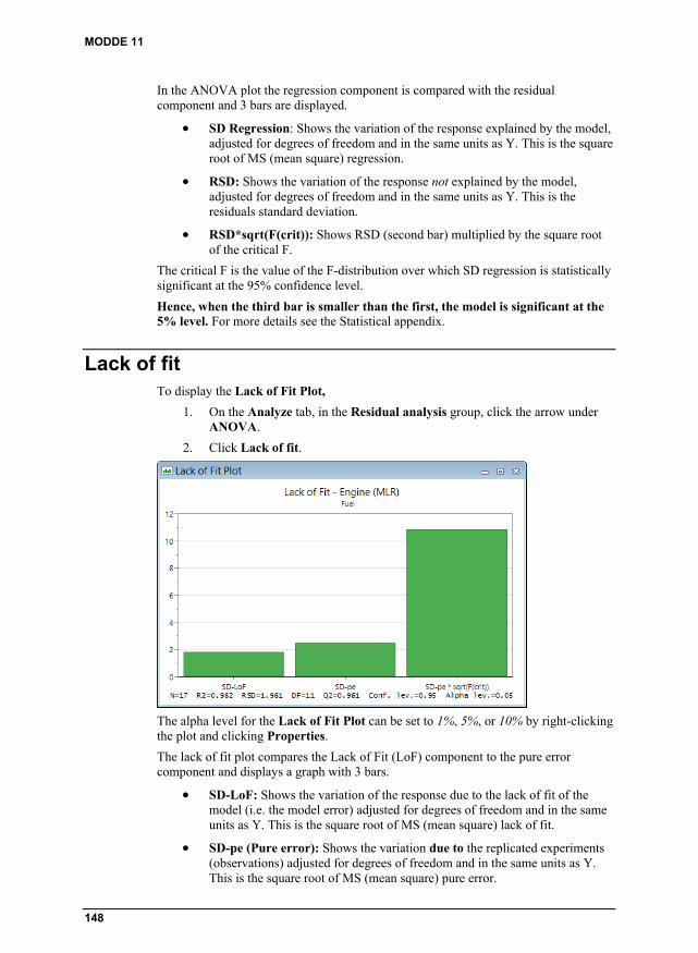
MODDE 11

148

In the ANOVA plot the regression component is compared with the residual component and 3 bars are displayed.

SD Regression: Shows the variation of the response explained by the model, adjusted for degrees of freedom and in the same units as Y. This is the square root of MS (mean square) regression.

RSD: Shows the variation of the response not explained by the model, adjusted for degrees of freedom and in the same units as Y. This is the residuals standard deviation.

RSD*sqrt(F(crit)): Shows RSD (second bar) multiplied by the square root of the critical F.

The critical F is the value of the F-distribution over which SD regression is statistically significant at the 95% confidence level.

Hence, when the third bar is smaller than the first, the model is significant at the 5% level. For more details see the Statistical appendix.

Lack of fit To display the Lack of Fit Plot,

1. On the Analyze tab, in the Residual analysis group, click the arrow under ANOVA.

2. Click Lack of fit.

The alpha level for the Lack of Fit Plot can be set to 1%, 5%, or 10% by right-clicking the plot and clicking Properties.

The lack of fit plot compares the Lack of Fit (LoF) component to the pure error component and displays a graph with 3 bars.

SD-LoF: Shows the variation of the response due to the lack of fit of the model (i.e. the model error) adjusted for degrees of freedom and in the same units as Y. This is the square root of MS (mean square) lack of fit.

SD-pe (Pure error): Shows the variation due to the replicated experiments (observations) adjusted for degrees of freedom and in the same units as Y. This is the square root of MS (mean square) pure error.

08-Analyze

149

SD-pe*sqrt(F(crit)): Shows SD pure error (second bar) multiplied by the square root of the critical F.

The critical F is the value of the F-distribution over which SD LoF is statistically significant at the 95% confidence level.

Hence, when the third bar is smaller than the first, the lack of fit is significant at the 5% level.

Box-Cox plot (MLR only) To open the Box-Cox plot, on the Analyze tab, in the Residual analysis group, click Box-Cox.

Note: The Box-Cox plot is only available when the model is fitted with MLR.

The Box-Cox Plot displays the maximum likelihood as a function of the power of the transformation by plotting values of lambda, λ, vs. the maximum likelihood.

If the response values vary more than a magnitude of ten in the experimental domain, a transformation is often recommended.

The maximum point on the Box-Cox plot gives the value of lambda, λ, for the response transformation Yλ that gives the best fit of the model. This is the maximum likelihood estimator for λ.

Box-Cox transform

MODDE displays λmax and its 95% confidence interval as λlower and λupper in the footer and on the plot as 3 vertical lines.

If λ=1 is included in that interval, then a transformation is not recommended.

If λ=1 is not included in the interval then Yλmax is the recommended transformation. You do not have to use the precise value of λmax but a near convenient value.

MODDE 11

150

Common transformations are:

λmax = -1, use the Power transformation and C3 = -1.

λmax = 0, use the Logarithmic (10Log) transformation.

λmax = 0.5, use the Power transformation and C3 = 0.5.

Residuals On the Analyze tab, in the Residual analysis group, click the arrow under Residuals.

This provides access to the following forms of displaying residuals,

Normal Probability Plot

vs. Predicted Response Plot

vs. Run Order Plot

vs. Variable Plot

List.

08-Analyze

151

Residual type Residuals can be displayed as Raw, Standardized, or Deleted studentized. The residual type can be changed by right-clicking the plot and clicking Properties.

Raw residuals

The raw residual is the difference between the observed and the fitted (predicted) value.

Standardized residuals

The standardized residual is the raw residual divided by the residual standard deviation (RSD).

Deleted studentized residuals

The deleted studentized residual is the raw residual (ei) divided by its standard deviation (si) where the standard deviation (si) is computed with observation (i) left out of the analysis, and corrected for leverage. Deleted studentized residuals require at least three degrees of freedom.

Note: Deleted studentized residuals are not available for PLS.

Default

With MLR and three or more real degrees of freedom (replicate degrees of freedom are not counted), deleted studentized residuals are the MODDE default when plotting residuals.

With PLS, MODDE uses the standardized residuals as default instead.

Residuals normal probability plot To display the Residuals Normal Probability Plot, on the Analyze tab, in the Residual analysis group, click Residuals.

MODDE 11

152

The residuals are plotted on a cumulative normal probability scale. This plot makes it easy to detect:

Normality of the residuals. If the residuals are normally distributed, the points on the probability plot follow close to a straight line.

Outliers. These are points deviating from the normal probability line, and having large absolute values of studentized residuals i.e. larger than 4 standard deviation indicated by red lines on the plot.

Residuals vs. predicted response To display the Residuals vs. Predicted Response Plot,

1. On the Analyze tab, in the Residual analysis group, click the arrow under Residuals.

2. Click vs. predicted response.

The plot shows the residuals vs. the fitted values. This plot is particularly useful to detect non-constant variance of the residuals. If the spread of the residuals increases with the fitted values, you may need to transform your response by taking its logarithm or its square root.

08-Analyze

153

Residuals vs. run order To display the Residuals vs. Run Order Plot,

1. On the Analyze tab, in the Residual analysis group, click the arrow under Residuals.

2. Click vs. run order.

This plot shows the residuals vs. run order (the order in which you performed the experiments) and helps you detect any dependency of the residuals on time.

Residuals vs. variable To display the Residuals vs. Variable Plot,

1. On the Analyze tab, click the arrow under Residuals.

2. Click vs. variable.

Right-click the plot and click Properties to select which variable to display on the x-axis.

MODDE 11

154

Residuals list To display the Residuals List,

1. On the Analyze tab, in the Residual analysis group, click the arrow under Residuals.

2. Click List.

The number under the response name is the experiment number.

Observed: The value of the response as listed in the worksheet.

Predicted: The predicted value for that observation.

Obs - Pred: The residual for that observation.

Conf. int: The 95% confidence interval on the predicted value. Right-click the list and click Properties to change the confidence level.

Observed vs. predicted To open the plot, on the Analyze tab, in the Residual analysis group, click Observed vs. predicted.

The Observed vs. Predicted Plot displays observed values vs. predicted values.

08-Analyze

155

Understanding the plot

Plots with points close to a straight line indicate good models. If Degrees of Freedom is under 3 (DF < 3), the plot will implicitly give a perfect fit.

Properties The properties dialog box of the Observed vs. Predicted Plot allows for the responses to be selected, limits to be shown or not, and what plot labels to display.

Coefficients There are two coefficient plots and two coefficient lists available in MODDE. To see the coefficient options, on the Analyze tab, in the Model interpretation group, click the arrow under Coefficients.

The coefficient plots provide graphical presentation of the significance of the model terms.

A significant term is one with a large distance from y=0 as well as having an uncertainty level that does not extend across y=0. A non significant model term is a model term close to y=0 and with an uncertainty level that crosses y=0.

MODDE 11

156

When confoundings are present, the coefficient plots and lists display a bracket # after the term. Hover your mouse pointer over the column to view the confounded terms.

Understanding the plot

The Coefficient plot presents a graphical representation of the model terms in order to determine their significance.

Significant model terms:

Far away from y=0 (either positive or negative)

Uncertainty range does not cross y=0.

Non significant model terms:

Close to y=0

Uncertainty range crosses y=0.

Remove non significant model terms from the plot

1. Click Exclude.

2. Find the least significant model term.

3. Check that no significant model term depends on the least significant model term.

4. Click the non significant model term to remove it.

5. Repeat steps 2-4 for as many model terms as required.

6. Click Exclude again.

Hint: Exclude only one model term at a time as it may make other model terms more significant. Q2 and DF (Degrees of Freedom) will increase as non significant model terms are removed, so note the before and after values as each term is excluded. A higher DF and Q2 is better.

Coefficient plot The Coefficient Plot displays the coefficients, when changing from 0 to high, for the selected response with the confidence interval as error bars. By default, the coefficients refer to the data scaled and centered.

08-Analyze

157

You can select which type of coefficient to display from Properties. Click Scaled and centered (default), Normalized, Unscaled, or PLS orthogonal (only available for PLS).

When you have confounded terms in your investigation these terms are marked with a bracket (#). Hover the mouse pointer over the column in the plot and you will get information about which terms it is confounded with. This information is available also in the coefficient overview plot.

Coefficient overview plot To make the coefficients comparable when responses (Y's) have different ranges, the coefficient overview plot displays the coefficients in Normalized form (the coefficients are divided by the standard deviation of their respective response). The Normalized mode is the default for the overview plot. You can change it to regular scale and centered coefficients by right-clicking and then clicking Properties.

The color for each factor is the same over all responses in the coefficient overview plot.

MODDE 11

158

Coefficient list The coefficient list displays the scaled and centered coefficients for the selected responses. P-values signaling non significant coefficients at the selected confidence level are colored red.

For the selected responses, this list includes:

Terms: Under the response name the name of the terms included in the model are listed. To display the list for another response, or more than one response, use the Response box or the list's Properties.

Coefficients: Value of the coefficient.

Standard error: Standard error of the coefficient.

P: Probability to get the displayed value for the coefficient assuming that the coefficient has a true value of zero.

Confidence interval: The 95% confidence interval on the coefficient value. To select a different level for the confidence interval, right-click the list and then click Properties.

Coefficient overview list The coefficient overview list displays the normalized coefficients for all the responses. Non significant coefficients at the selected confidence level are shown in red.

Note: The Coefficient overview list is only available when all responses are fitted to the same model, that is, when the same model terms are included for all responses.

08-Analyze

159

Effects In MODDE you can create three different effect plots:

Effect Plot: Displays the effect calculated as twice the MLR coefficient and sorted descending in absolute value.

Effects Normal Probability Plot: Displays the effects on a normal probability scale.

Main Effect Plot: Displays predicted values of the selected responses, when the factor varies from its low to its high level.

The Effect List displays the effects and their confidence intervals.

Note: When an expanded list of the qualitative levels is desirable, use the coefficient plots and lists to display the coefficients for every level of a qualitative variable instead of the effect plots and lists. Note that the effects for linear and interaction models are twice the corresponding coefficients.

Accessing effects plots and list To open an effects list or plot,

1. On the Analyze tab, in the Model interpretation group, click the arrow under Effects.

2. Click the desired plot or list.

Effect plot For process factors the values of the effects (computed as twice the MLR coefficients) are plotted sorted (in absolute value) in descending order. The ± 95% confidence interval is shown as error bars. The confidence level can be changed in the Effect Plot dialog box (right-click the plot and click Properties).

MODDE 11

160

For mixture factors this plot displays the adjusted Cox effects (unavailable for Scheffé models). This effect represents the change in the response values when component k varies over its range, all other mixture factors kept in the same proportion as in the reference mixture.

For details on how the mixture effects are calculated, see the Statistical appendix.

Effects normal probability plot The plot displays the effects plotted on a cumulative normal probability scale.

This plot should only be used when the model is saturated (a model with as many terms as experimental runs). For saturated models MODDE cannot compute standard errors, p values and confidence intervals. Use the plot to help determine the important effects.

08-Analyze

161

This plot, proposed by Daniel in 1954, is based on the fact that if all estimated effects were noise, they would have a normal distribution and when plotted on a normal cumulative plot, would fall on a straight line. Hence effects significantly different from zero (noise) will fall outside the normal line.

This plot assumes independent effects, and that all estimable effects are plotted. Hence, it is only relevant for screening designs with saturated models DF = 0. Also for this plot to be meaningful, models need to have at least 10 effects. If these conditions are not met MODDE will warn that this plot may not be statistically correct.

Note: The normal probability of effects plot is not available with mixture factors.

Main effect plot For process factors the plot displays the predicted values of the selected response, when the factor varies over its range, all other factors in the design held constant at their averages. Qualitative factors held constant are set at their numerical average and do not influence the predicted values.

If the design has replicated center points for the displayed factor, where the other factors are also at their averages, the observed values of these points are colored differently from other worksheet points.

The points displayed in this plot are the worksheet data, current factor vs. response, not taking into account the other factor settings.

To hide the worksheet data, right-click the plot, click Properties, and on the Options tab clear the Worksheet data check box.

Main effect plot for mixture factors

When you select to display a mixture factor Xk, this plot displays the predicted change in the response when Xk varies from its low to its high level, the relative amounts of all other mixture factors are kept in the same proportion as in the standard reference mixture.

For details, see the Statistical appendix.

MODDE 11

162

Switching displayed factors

To switch factors,

1. Right-click the plot,

2. Click Properties,

3. Click the Select factor tab,

4. Select the desired factor,

5. Click OK.

Formulation factors can be adjusted proportional to the reference mixture or ranges on this property page.

Effect list The values of the effects (twice the coefficients) are listed with their 95% confidence interval sorted (in absolute value) in descending order. The confidence level can be changed in the Properties dialog box for the Effect List (right-click the plot and click Properties).

08-Analyze

163

Interactions To open the interaction plot, on the Analyze tab, in the Model interpretation group, click Interactions.

To switch to another interaction and/or switch the factor displayed on the x-axis:

1. Right-click the plot and click Properties.

2. In the Interaction effects tab, click the term in the Interaction term box and/or select the factor in the Factor on X-axis box.

Note: This plot is only available for process factor. No interaction plots are available for mixture factors.

When you select a 2 factor interaction, the predicted values of the response, when one factor varies from its low to its high level, are plotted for both levels of the other factor, all remaining factors in the design being set on their average.

If you have mixture factors in the model, these are all set at the standard reference mixture.

PLS The score and loading plots complement each other. The position of an observation in a given direction in a score plot is influenced by variables lying in the same direction in the loading plot.

There are four types of PLS plots available:

Score Scatter Plot – displays the score vectors t and/or u in a scatter plot. Use the score plots to reveal groups, trends, outliers, and similarities. The plot marks represent your experiments.

Score Column Plot – displays the score vectors t or u in a column plot.

MODDE 11

164

Loading Scatter Plot – displays the loading vectors p, c, w and/or wc in a scatter plot. Use the loading plots to investigate the correlation between terms in your model. The plot marks represent the terms currently in the model and/or the response-variables. The response variables are displayed when plotting the c-vectors.

Loading Column Plot – displays the loading vectors p, c, w or wc in a column plot.

Accessing PLS plots

To access the PLS plots, on the Analyze tab, in the PLS diagnostics group, click the arrow under PLS.

This shows the available PLS plots.

Score plots The score plots reveal groups, trends, outliers, and similarities.

You can create three different score scatter plots:

T scores (for ex.: t1 vs. t2): t scores are windows in the X space displaying the objects as situated on the projection plane or hyper plane.

U scores (for ex.: u1 vs. u2): u scores are windows in the Y space, displaying the objects as situated on the projection plane or hyper plane.

T vs. U scores (for ex.: t1 vs. u1): Displays the objects in the projected X (T) and Y (U) space, and how well the Y space coordinate (u) correlates to the X space coordinate (t). This is the default.

Score column plots can only be created for one vector at a time.

Note: Score plots are only available for PLS fitted models.

Loading plots The loading plots display the correlation between the X variables T(X) and the Y variables U(Y).

Note: Loading plots are only available for PLS fitted models.

08-Analyze

165

You can create four different loading plots:

p loadings (for ex.: p1 vs. p2): These plots show the importance of the X variables in the approximation of the X matrix.

w loadings (for ex.: w1 vs. w2): The w's are the weights that combine the X variables (first dimension) or the residuals of the X variables (subsequent dimensions) to form the scores t. These weights are selected so as to maximize the correlation between T and U, thereby indirectly Y. X variables with large w's (positive or negative) are highly correlated with U (Y). Variables with large w's are situated far away from the origin (on the positive or negative side) on the plot.

c loadings (for ex.: c1 vs. c2): These plots display the correlation between the Y variables and the X scores T (X). The c's are the weights that combine the Y variables with the scores u; so as to maximize their correlation with X. Y variables with large c's are highly correlated with T (X).

wc loadings (for ex.: wc1 vs. wc2): This is the default option. These plots show both the X-weights (w) and Y-weights (c), and thereby the correlation structure between X and Y. One sees how the X and Y variables combine in the projections, and how the X variables relate to Y.

To change the currently showing loading plot,

1. Right-click the loading plot

2. Click Properties

3. On the Loading Column Plot or Loading Scatter Plot tab, click the desired option

4. Click OK.

Loading column plots can only be created for one vector at a time.

Distance to model (Y) To open the distance to model plot, on the Analyze tab, in the PLS diagnostics group, click Distance to model.

The RSD of an object in the Y space is proportional to the object distance to the hyper plane of the PLS model in the Y space. MODDE computes the object distance to the PLS model (DModY) in the Y space and displays them as columns in a plot.

A large DModY value indicates that the experiment may be an outlier.

MODDE 11

166

VIP - Variable importance in the projection The VIP values reflect the importance of terms in the model both with respect to Y, i.e. its correlation to all the responses, and with respect to X (the projection). With designed data, i.e. close to orthogonal X the VIP values mainly reflect the correlation of the terms to all the responses.

Note: The VIP plot and VIP list are only available for PLS fitted models.

VIP plot

The VIP plot displays the VIP values as a column plot sorted in descending order.

To open the VIP Plot, on the Analyze tab, in the PLS diagnostics group, click VIP.

08-Analyze

167

VIP list

The VIP list displays the sorted VIP values and the scaled and centered coefficients for all responses in the investigation.

To open the VIP List,

1. On the Analyze tab, in the PLS diagnostics group, click the arrow under VIP.

2. Click VIP list.

169

09-Predict

Introduction The Predict tab has a collection of functions that involve predictions and interpretation, as well as the Optimizer.

The functions on the Predict tab are organized into groups,

Spreadsheet group

Predictions - opens the Prediction Spreadsheet.

Scatter - opens the Prediction Scatter Plot dialog box for creating 2D or 3D scatter plots using the content of the Prediction Spreadsheet.

Interpretation group

Prediction plots - creates prediction and overlay prediction plots.

Factor effects - shows the Factor Effect Plot for the currently selected responses.

Contour - opens the Contour Plot dialog box to create Contour, 4D contour, and Surface plots.

Sweet spot - creates Sweet spot, 4D sweet spot, and Surface plots.

Design space - opens the Design Space Plot dialog box for creating Contour and 4D contour plots.

Optimize group

Optimizer - opens the optimizer window and provides access to the Optimizer contextual tab.

Setpoint validation - opens the Setpoint Validation window.

MODDE 11

170

Prediction spreadsheet The Prediction Spreadsheet allows you to type or paste factor settings to make predictions. The lower and upper level 95% confidence intervals for these predictions are also calculated.

To open the Prediction Spreadsheet, on the Predict tab, click Predictions.

To insert rows press the Down arrow key when on the last row.

If the model has been fitted the predictions are calculated automatically after entering settings for all factors. If you do not want the predictions to be automatically updated, right-click the list and clear Auto update. To make predictions with auto update cleared, right-click the list and click Update predictions or press the F5 key.

To change the interval estimation properties, right-click the list and click Properties and click the Interval estimation tab.

Note: With PLS and an X matrix with large condition number, the standard error of predictions is computed and displayed instead of the interval estimate.

Prediction scatter plot In the prediction scatter plot you can view your factors and predicted responses as 2D and 3D scatter plots.

Note: The points displayed in the scatter plots are the points in the current prediction spreadsheet. The scatter plot is updated with new points when you enter them in the prediction spreadsheet.

To create a prediction scatter plot, on the Predict tab, click Scatter Plot. This will open up the Prediction Scatter Plot dialog box.

09-Predict

171

To add a variable to an axis or series, click the variable in the Column field, then click

the relevant arrow . Click to remove factors or responses from the Y-axis or from Series. To change what to display on the X-axis, mark a new variable and

click .

For 2D plots, select the variable to be plotted on the X and Series (Z) axes.

For 3D plots, select the variables to be plotted on the X, Y, and Series (Z) axes.

Click the Color by variable tab to color by a factor or a response.

Prediction plots There are two prediction plots available for process and two prediction plots available for mixture.

On the Predict tab, in the Interpretation group, click the arrow under Prediction plots.

MODDE 11

172

Right-click any prediction plot and click Properties to:

Select the responses on the Select responses tab. You can also use the Select response box.

Select which factor to display on the x-axes on the Axes and constants tab.

Select interval estimation settings - Interval type, Confidence level, Tolerance proportion on the Interval estimation tab.

Select if limits should be shown in the plot or not on the Options tab.

Select if worksheet raw data points should be show or not on the Options tab.

Use the Properties pane factor sliders to interactively change the settings of the constant factors.

Prediction plot The prediction plot displays the predicted values of the selected responses, when the factors vary over their respective ranges. The plot supports up to three factors and an unlimited number of responses with confidence intervals when the Show interval estimates check box is selected. The plot also displays any worksheet points that are valid considering the constant settings of the factors not displayed on the axes in the subplot but in the Properties pane. The tolerance for the constant factors is specified by the replicate tolerance in MODDE options.

Overlay prediction plot The overlay prediction plot displays the predicted values for up to three factors and as many responses as desired. No confidence intervals can be displayed for the overlay plot.

09-Predict

173

Factor effects To access the Factor Effect Plot, on the Predict tab, in the Interpretation group, click Factor effects.

For process factors the plot displays the predicted values of the selected responses, when the factor varies over its range, all other factors in the design held constant at their averages. Qualitative factors held constant are set at their numerical average and do not influence the predicted values.

The points displayed in this plot are the worksheet data, current factor vs. response, not taking into account the other factor settings.

To hide the worksheet data, right-click the plot, click Properties, and on the Options tab clear the Worksheet data check box.

MODDE 11

174

Note: The Factor Effect Plot by default shows both factors and the responses back transformed (in original units) while the Main Effect Plot shows the responses in their transformed units.

Factor effect plot for mixture factors

When you select to display a mixture factor Xk, this plot displays the predicted change in the response when Xk varies from its low to its high level, the relative amounts of all other mixture factors are kept in the same proportion as in the standard reference mixture.

For details, see the Statistical appendix.

Switching displayed factors

To switch factors,

1. Right-click the plot,

2. Click Properties,

3. Click the Select factor tab,

4. Select the desired factor,

5. Click OK.

Formulation factors can be adjusted proportional to the reference mixture or ranges on this property page.

Factor effects, Stability designs To access the Factor Effect Plot, on the Predict tab, in the Interpretation group, click Factor effects.

For stability designs the plot by default displays the predicted values of the selected response, when the Time factor varies from first to last time. All other factors in the design are held constant at their averages. Qualitative factors held constant are set at their numerical average and do not influence the predicted values.

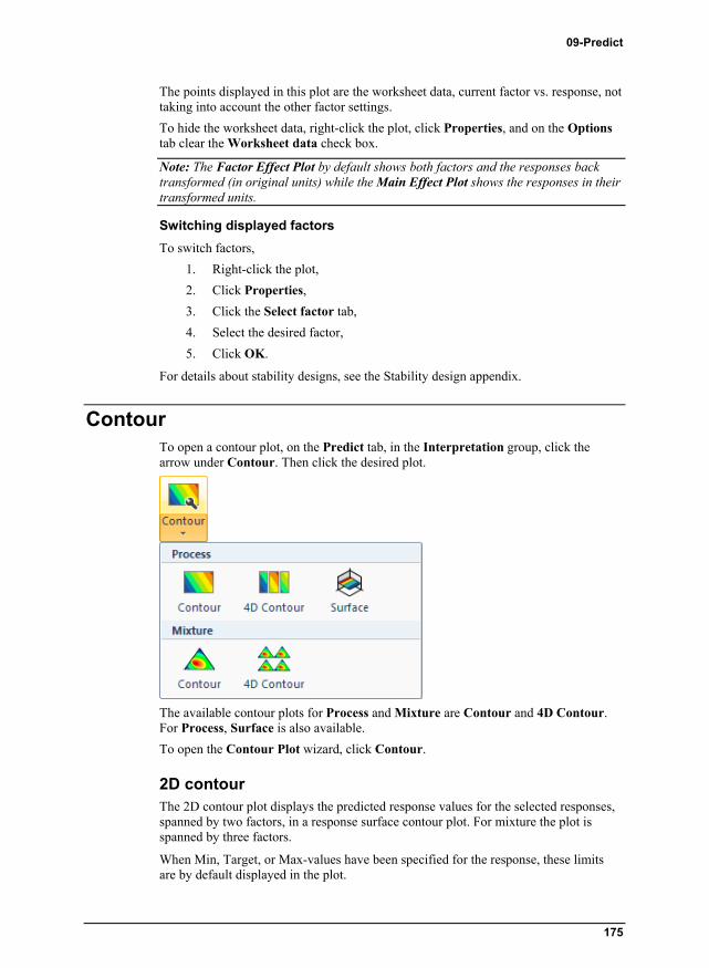
09-Predict

175

The points displayed in this plot are the worksheet data, current factor vs. response, not taking into account the other factor settings.

To hide the worksheet data, right-click the plot, click Properties, and on the Options tab clear the Worksheet data check box.

Note: The Factor Effect Plot by default shows both factors and the responses back transformed (in original units) while the Main Effect Plot shows the responses in their transformed units.

Switching displayed factors

To switch factors,

1. Right-click the plot,

2. Click Properties,

3. Click the Select factor tab,

4. Select the desired factor,

5. Click OK.

For details about stability designs, see the Stability design appendix.

Contour To open a contour plot, on the Predict tab, in the Interpretation group, click the arrow under Contour. Then click the desired plot.

The available contour plots for Process and Mixture are Contour and 4D Contour. For Process, Surface is also available.

To open the Contour Plot wizard, click Contour.

2D contour The 2D contour plot displays the predicted response values for the selected responses, spanned by two factors, in a response surface contour plot. For mixture the plot is spanned by three factors.

When Min, Target, or Max-values have been specified for the response, these limits are by default displayed in the plot.

MODDE 11

176

Factors kept constant

By default, all constant factors are set at their mid-range values; change these values as desired in the Properties dialog or pane. After the plot has been created the constant factors can be seen (and changed) by clicking the Properties tag to the right of the plot to open the pane. When you change the value of the constant factors, the contour plots are updated.

4D contour The 4D Contour plot displays the predicted response values for the selected response, spanned by two factors, in 9 response surface contour plots in a 3x3 grid and spanned by another two factors. For mixture, the plots are spanned by three factors.

When Min, Target, or Max-values have been specified for the response, these limits are by default displayed in the plot.

Note: The 4D plot is available for investigations with only process factors, and with both mixture and process factors, but not with mixture factors only.

4D contour plot axes

When the model includes both process and mixture factors, the mixture factors can only be selected as inner axes factors in the Contour Plot wizard.

Inner axes factors

Select two process factors for the axes under Factors at the plot axes, or three mixture factors.

Outer axes factors

Select two process factors for the outer axes. The response contours are plotted for the low, middle, and high levels of these factors.

You can also select qualitative factors for the outer axes and select for which settings to display the contour plots.

09-Predict

177

When there are more than 4 factors in the model, the remaining factors are held constant.

By default all plots are equally scaled, that is, the color coding is the same for all plots.

Response surface The Response Surface Plot displays the predicted response values, spanned by two factors, in a response surface plot. This plot is only available for models with two or more process factors and can display many responses.

Factors kept constant

By default, all constant factors are held constant at their mid-range values; change these values as desired. After the plot has been created the constant factors are found to the right in the plot. When you change the value of the constant factors the contour surface plot is updated.

MODDE 11

178

Surface plot options

The plot options for the response surface plot are, as the Contour plot options, accessed by clicking Plot options in the Contour Plot wizard, or in tab Surface plot options in the properties dialog after creating the plot.

The Surface plot options include two options:

Resolution - The precision used when creating the contour plot. Selecting a higher resolution requires more calculations and is therefore more time consuming. To select the resolution of the plot, click one of the predefined resolutions or type a resolution value here.

Scale surfaces 0-100 - How to scale the response axis. When selected (as in the example here), each response is scaled so that the smallest predicted value equals 0 and the largest predicted value equals 100. Note that with Min, Target and/or Max values in the response definition, these values are included in range used to rescale, possibly increasing that range. As a consequence the scale of the actual surface is less than 0-100 when a Min/Target/Max-value increases the range.

Contour plot wizard The contour plot wizard guides you through the selection and specification of 2D contour plots and 4D contour plots for mixture and process factors and 2D Surface plots for process factors.

To open the contour plot wizard, on the Predict or Home tab, click Contour.

09-Predict

179

Inner plot type

Under Inner plot type, the default plot type for the inner axes is selected. If you have both process and formulation factors in the investigation, click the type of factor to display on the inner axes: Process or Mixture.

On the outer axes you can only vary process factors.

Selecting responses

You can select to display all responses for the 2D contour plots but with more than 9 responses, the plots become very small. The contours are not overlaid, but displayed next to each other.

Modify which responses to display by marking in Available responses and clicking

the arrow and/or marking in Selected responses and clicking the back arrow

.

Using constraints

Clear the Use constraints check box if you do not want the available constraints to be displayed in the plot. MODDE's default is for constraints to be used and this should not be changed without reason.

Plot options

To select the resolution of the plot, that is, the grid calculated to create the contour plot, click Plot Options. Note that you can type a resolution value here or click one of the predefined resolutions.

You can also scale the subplots equally, to lock the contour levels, to produce the plot with/without color and with/without contour level labels.

For more, see the Contour plot options subsection.

MODDE 11

180

Contour plot options Right-click the contour plot and click Properties to open the property page. The features described here can also be accessed by clicking Plot options in the Contour plot wizard.

Resolution

Resolution is the precision used when creating the contour plot. Selecting a higher resolution requires more calculations and is therefore more time consuming.

To select the resolution of the plot, click one of the predefined resolutions or type a resolution value here.

Scale subplots equally

When the Scale subplots equally check box is selected the colors of all contour subplots represent the same values.

The plot has subplots when you display the 4D contour or you have selected to display more than one response in the 2D contour plot.

Lock contour levels

You can select the Lock contour levels check box to keep the current contour level colors and limits.

This option is available when the Scale subplots equally check box has been selected.

Use color

By clearing the Use color check box you can choose to display the contour and surface plots without colors.

Show contour level labels

Clear the Show contour levels labels check box to display the contour plots without the level labels.

Sweet spot The Sweet Spot plot highlights the areas were the responses are within the user specified ranges but does not add the probability assessment that is done by the Design Space plot. The sweet spot plot can be displayed as 2D or 4D for process or mixture factors. For process factors the plot can also be displayed as a surface where the response intersections are viewed in 3D.

09-Predict

181

Creating a sweet spot plot To open the sweet spot plot wizard, on the Predict tab, click Sweet spot.

Inner plot type

If the investigation contains both mixture and process factors, select the type of factor you want on the axes for the 2D and for the inner axes for the 4D.

Plot type

To select to create the 2D sweet spot plot select Sweet spot and to select the 4D with up to four factors (5 with mixture) click 4D sweet spot. To create a sweet spot surface, click Surface. Click Next.

Response selection

In the Responses page, enter the settings for the relevant responses.

Note: If you have entered Min and/or Max values in the response definition, this page is automatically filled with those values. To update with updated values from the response definition, click Get limits.

MODDE 11

182

For each response select:

1. To Include or Exclude each response under Incl/Excl.

2. Type the values that are of interest under Min and Max. If you have entered the Min and Max yourself, MODDE uses those values. If you have not specified a Min and Max, MODDE enters the smallest and the largest values found in the worksheet and these should be changed based on your desired sweet spot.

You may also:

Select or clear the Use constraints check box.

Change the resolution in the Resolution box.

Update to current limits in the response definition by clicking Get limits.

Plot axes

Click Next to open the Axes and constants page, or for 4D sweet spot, the 4D axes page.

Mixture factors can only be selected as inner factors in a 4D plot.

09-Predict

183

Select two process factors for the axes under Factors at the plot axes, or three mixture factors.

For the 4D, select two process factors for the outer axes. The sweet spot contours are plotted for the low, middle, and high levels of these factors.

Colors in the sweet spot plot

The sweet spot plot uses the color scale from green to blue with:

Green for the ‘sweet spot’, that is the areas where all responses are within the selected range.

Blue for areas where one of the responses is within its selected range.

White for areas where none of the responses are within their selected ranges.

Other colors for areas with more than one response within its range but not all.

The above are the default settings and you can define specific colors in the Format Plot dialog box.

MODDE 11

184

Design space On the Predict tab, in the Interpretation group, click Design space to open the Design Space Plot dialog box with settings for creating the plot. Click the arrow under Design space to open a specific design space plot directly.

Available options are:

Process

Design space

4D design space

Mixture (only available when mixture factors are part of the design)

Design space

4D design space

09-Predict

185

Design space wizard The Design Space Plot wizard opens automatically when clicking Design space on the Home or Predict tabs.

First page The first page of the Design Space Plot wizard lets you choose;

Plot type - either Contour or 4D contour.

Inner plot type - Process or Mixture.

Selected responses - As many as desired.

Plot options - see the Design space plot options subsection next.

Design space plot options

Click Plot options... on the first page in the wizard to open the plot options, alternatively right-click the created plot and click Properties. The Design Space Contour Options lets you specify,

Resolution - A higher resolution means a more detailed plot, but it can also slow down your computer.

Use color - This determines if the plot should be colored or merely display the contour lines.

Show contour level labels - Select to display contour level labels.

Output - Choose between Probability of failure (%) and Probability of failure (DPMO). Probability of failure (%) is default selected.

Limit - The acceptance criteria to aim for either in percentage or in the DPMO space.

MODDE 11

186

Simulations/point - The number of simulations per point; the higher the more time consuming but also more accurate.

Include model error - This determines if model error should be included in the plot. Note that when this check box is cleared, the plot merely presents the same information as the Sweet spot plot.

Interval type, Confidence level and Tolerance proportion on the Interval estimation tab. For more, see the Interval type and probability levels subsection in chapter 4, File.

4D axes The second page of the wizard lets you select what factors to display on each of the plot axes. In Distribution, the type of distribution can be selected; Normal (default), Uniform or Triangular.

09-Predict

187

Note: When creating the plot from the Setpoint analysis group on the Optimizer tab, you can also select to include distribution from the setpoint analysis on the axis factors and if you want to include distribution from setpoint analysis on constant factors.

Click Finish to see the Design Space Plot showing the probability of failure (%) for the shown factor combinations. Alternatively, Next to specify the settings for the constant factors.

Optimizer On the Predict tab, in the Optimize group, click Optimizer to open the Optimizer window and provide access to the Optimizer contextual tab.

More information about the optimizer is available in Chapter 12, Optimizer.

Setpoint validation On the Predict tab, click Setpoint validation to open the Setpoint Validation window.

Setpoint validation tests the robustness by making a large number of random disturbances (Monte Carlo simulation) in the specified region. The result is shown as a distribution of random samples including model prediction errors. The result can be expressed in general statistics as well as capability indices Cpk or DPMO = Defects Per Million Opportunities outside specifications.

Setpoint validation is a way to test if the investigated system is robust against disturbances in the investigated region.

MODDE 11

188

The aim of robustness testing is to evaluate if a process, or a system, performs satisfactory even when some influential factors are allowed to vary. In other words, we want to investigate the system’s sensitivity (or preferably lack of sensitivity) to changes in certain critical factors. The advantages of a robust process or system include simpler process control, a known range of applicability and an ensured quality of the product or process.

A robustness test is usually carried out before the release of an almost finished product, or analytical system, as a test to ensure quality. MKS Umetrics recommends the use of DoE for robustness testing and such a design is usually centered on the factor combination, which is currently used for running the analytical system, or the process. We call this the setpoint. The setpoint may have been found through a screening design, an optimization design, or some other identification principle, such as written quality documentation. The aim of robustness testing is, therefore, to explore robustness close to the chosen setpoint.

The regression model originates from a low resolution design supporting linear models since we assume that small disturbances have mainly linear effects. Fractional factorial resolution III and Placket Burman designs are recommended.

Setpoint validation plots and lists The Setpoint validation features available for working with setpoint diagnostics are;

Factor distribution

Response distribution

Setpoint summary.

For more information on these functions, see Chapter 13, Setpoint.

189

10-View

Introduction The View tab offers a selection of options for changing what windows are visible as well as choosing how to display open windows.

The available functions include,

Show - Toggles the visibility of sections of MODDE such as the Status bar and Analysis advisor.

Full screen - Enter full screen mode.

Window - Rearrange, close, or swap between MODDE's windows.

Show On the View tab in the Show group it is possible to choose to show or hide the following parts of the window:

Analysis advisor - The Analysis Advisor pane is automatically activated after fitting an investigation. The advisor explains a selection of the plots and results available in MODDE.

Audit trail - for details, see the Audit trail subsection later in this chapter.

Favorites - for details, see the Favorites section later in this chapter.

Output - The Output pane is a log book of the session. All MODDE messages and actions are recorded in the logbook.

Notes - In the Notes pane you can record your own notes concerning the investigation. You can paste MODDE plots and lists. Note the commands available by right-clicking the window. This file can then be saved as .rft (Rich Text Format) and read directly by a word processor with all plots.

Status bar - Displays details about the current investigation. Note that clicking the information opens a list/spreadsheet or dialog box. For instance, clicking Factors opens the Factors spreadsheet, clicking Objective opens the Design Wizard on the Select objective page.

MODDE 11

190

All of the items above (with the exception of the status bar) can be moved around to other sections of the viewable area by clicking and dragging them. To make the windows smaller, pull the top/side and it will remember its size. Double-click the window caption to make it floating or make it dock.

Hint: While dragging the window hold down the CTRL key. It won't dock if you are close to the frame of the main frame window.

Audit trail When the Audit Trail is turned on each investigation in MODDE has a separate audit trail. Each audit trail consists of one or more sessions that in turn consist of events. A new session is started and appended to the audit trail when an investigation is opened, and ends when the investigation is saved.

In addition to logging events, MODDE logs information about the user, and date and time of the events.

To view the audit trail, click the Audit Trail tab in the Output / Notes / Audit trail pane. If this tab is not shown, display it by selecting the Audit Trail check box on the View tab.

Enable and disable the Audit Trail

By default the audit trail is disabled.

To turn it on for the current investigation, in File | Options, on the Investigation options page, under Audit trail, select Yes in Enable the audit trail.

To turn on the audit trail for new investigations, in File | Options, on the MODDE options page, under Audit trail, select Yes in Enable the audit trail for new investigations.

Administrators can disable the turning on and off of the audit trail, i.e., always have it on or off. For instructions on how to disable the audit trail options, see the knowledge base at www.umetrics.com.

Save or clear the Audit Trail

To empty the audit trail, in the Audit Trail pane, right-click and click Clear Audit Trail.

To save the current version of the audit trail, separate from the investigation, in XML format, in the Audit Trail pane, right-click and click Save as.

Audit trail and internet explorer

MODDE uses Internet Explorer functionality to display the audit trail.

Logged in the audit trail

Specific actions the MODDE audit trail logs are:

Factors (adding, modifying, deleting), displaying all details about the factor after the change

Responses (adding, modifying, deleting), displaying all details about the response after the change

Constraints (modifying, deleting)

10-View

191

Candidate set

Inclusions

Reference mixture

Objective

Generators

Design

Complement design

Model

Worksheet, every change of every cell

Fit method

Activation and deactivation of the Audit Trail.

The audit trail also registers when a digital signature in the Audit trail is incorrect.

Favorites

Introduction To open or close the Favorites pane, on the View tab, select the Favorites check box.

The Favorites pane by default includes a few plots, lists and spreadsheets and can be extended and modified as desired.

Open a plot or list by clicking it. When settings must be selected, a dialog box opens; select the appropriate settings and click OK. Plots and lists are displayed with the selected settings.

Almost all plots in MODDE can be added to favorites.

Adding favorites

To add an open plot or list to favorites, on the Tools tab, click Add to favorites or right-click and click Add to favorites. Note that this adds the plot with the selected settings to the Favorites pane.

MODDE 11

192

Opening favorites

To open a favorite, double-click it or mark it, right-click and click Open.

Right-clicking the Favorites pane opens the menu below. A description of the menu items follows.

Open all items in folder – Executing a folder

To execute all commands in a folder, right click the folder and select Open all items in folder.

For example with the default Analysis folder, opening all items in the folder displays the replicate, summary of fit, residuals normal probability, coefficient and observed vs. predicted plots for the first response tiled.

Treat folder as item

Click Treat folder as item to treat the folder as an item. The folder is then displayed as an item:

Click it to open all the items. This gives the same result as Open all items in folder but with a single click.

Rename

All folders, plots, spreadsheets, and lists can be renamed according to your wishes by right-clicking it and clicking Rename, or marking it and pressing the F2-key on your keyboard.

Delete

All items in Favorites can be deleted by right-clicking the item and clicking Delete, or marking it and pressing the DELETE-key on your keyboard.

Create a new folder

It is convenient to group commands in folders, and automatically execute all the commands in the folder in sequence. To create a folder in Favorites, right-click and click New folder.

The created folder is default named 'New folder'; change the name as desired, for example to 'Residuals Plots'.

To move favorites to the Residuals Plots folder, use the drag-and-drop feature.

Importing and exporting Favorites configuration

The Favorites window configuration can be saved as an .xml-file.

10-View

193

To save the current favorites configuration to file:

1. Right-click the Favorites window.

2. Click Export.

3. Enter the name and location in the Save As dialog,

4. Click Save.

Note: When importing a favorites file, the new favorites will replace the current favorites. If you want to keep you current configuration and switch back to it later, export to file before importing a new one.

To import favorites from .xml-file:

1. Right-click the Favorites window.

2. Click Import.

3. Browse for the file in the Open dialog.

4. Click Open.

Restoring favorites

To restore Favorites to the MODDE default, on the File tab, click Options and on the Restore page click Restore in the Favorites section.

Full screen You can use the Full screen command to maximize the plot area. Full screen can be toggled on and off using F11 and is available on the View tab. Use F11 to leave full screen mode.

Window On the View tab in the Window group there are icons to choose how open windows are arranged;

Cascade windows,

Tile horizontally,

Tile vertically.

Close Clicking Close closes the active window. Clicking the arrow under Close offers other close options;

Close all windows,

Close all but active,

Close all plots,

Close all lists.

MODDE 11

194

Switch windows Switch windows offers a list of open windows. The selected window will be brought to the front.

The Switch windows function also offers an option to Arrange windows. Selecting this brings up the Arrange Windows dialog box where you can select a specific window to bring to the front (Activate) or to close or minimize selected windows. If you select more than one window (using the normal windows method of Shift or Ctrl to select multiple items) the Cascade, Tile Horizontally and Tile Vertically options become available.

195

11-Tools

Introduction The Tools tab provides functions to interact with the currently selected plot or list. If a function is not available for the active plot or list, it will also be unavailable on the tab.

The functions are organized into groups as follows,

Layout group

Add plot element - add or remove elements such as headers and footers to the currently selected plot.

Templates - save or load a template.

Plot tools group

Select - selection tool, such as free form, or x-axis.

Zoom - Zoom in, zoom X, zoom Y, zoom subplot.

Zoom out - zooms out if zoomed in.

Screen reader - get the coordinates from a specific point on a plot.

Exclude - turn on/off exclude mode or exclude selected data.

Create group

List - creates a list for the active plot.

Document group

Add to favorites - add the currently active plot or list to the favorites list.

Add to report - add the currently selected plot or list to a report.

Format plot - opens the Format Plot dialog box.

Add plot element Add or remove plot elements such as headers, footers, and legend.

MODDE 11

196

To add new plot elements to a plot:

1. On the Tools tab, in the Layout group, click Add plot element.

2. Select the desired plot elements.

Alternatively:

1. Click the plot window to make the mini toolbar appear.

2. Click the add plot element icon .

Available plot elements

Header

Footer

Legend

Axis titles

Axes

Regression line

Timestamp.

Templates On the Tools tab, in the Layout group, click Templates to display options to save, load, and manage plot templates.

The plot template specifies the visualization of the plots (fonts, colors and sizes for headers, background color, legend alignment, etc.).

Save template - You can choose to save the current template under the current name, as default, or as anything else. Note that the Default template is marked, even if change have been introduced, until you save the template under a different name.

Load template - Choose between previously saved templates or the default template. The current template is marked.

11-Tools

197

Manage templates - Open the templates folder for browsing or Restore default settings. Restore default settings restores and switches to the settings that MODDE had when installed, not changing any custom templates.

Select On the Tools tab, in the Plot tools group, click the arrow under Select to view available selection methods.

Free-form selection Click a plot area with the left mouse button and drag to create a free form selection area. Release the mouse button to select everything within that area.

Rectangular selection Click a plot area with the left mouse button and drag to create a rectangular selection area. Release the mouse button to select everything within that area.

Select along the X-axis Click a plot area with the left mouse button and drag left or right, along the x-axis. Release the mouse button to select everything within that area.

MODDE 11

198

Select along the Y-axis Click a plot area with the left mouse button and drag up or down, along the y-axis. Release the mouse button to select everything within that area.

Move points When the active plot is the Dynamic profile, the Move points option is available. Click a point with your left mouse button and drag the point to the desired location. Release the mouse button and the Dynamic profile plot and the Optimizer window will update with the new Setpoint location.

Zoom and zoom out To zoom in or out in a plot, Zoom and Zoom out are available on the Tools tab in the Plot tools group. Click the arrow under Zoom to access the different zooming options.

To undo the zoom and return to the previous zoom level, click Zoom out.

Zoom subplot by activating the zooming tool and double-clicking the subplot.

Zoom and rotate 3D plots Turn the 3D scatter plot or response surface plot by holding down the left mouse-button and moving the mouse in the direction you want to turn the plot.

Zoom in or out in the plot by using the mouse wheel.

To reset the rotation to default, right-click and click Reset rotation.

11-Tools

199

Screen reader On the Tools tab, in the Plot tools group, click Screen reader to change the select tool to the screen reader tool. This presents information relevant for that specific plot at the point the mouse pointer is located.

Exclude Exclude is located on the Tools tab, in the Plot tools group and in the Editing group on the Home tab.

Use Exclude to remove unwanted model terms or experiments from plots and charts. Exclude can either be clicked before selecting points or after selecting points. When clicked before selecting points, Exclude remains active allowing for the repeated removal of model terms.

Click Undo to readd newly removed model terms or experiments.

Format plot Format plot allows for you to change plot details such as the legend, error bars, columns, styles, gridlines, background, etc. The options available when using format plot depend on the plot that is currently active. The Format Plot dialog box provides options for completely changing the look of your plot. Everything from the footer, timestamp, headers, subheaders, shape of the points, etc can be changed. MODDE allows you to completely customize your plots so that they will best fit into your report. Any element in a plot that you can click, can likely be customized.

Accessing format plot To access the format plot options for the currently active plot,

On the Tools tab, click Format plot.

Right-click a plot and select Format plot from the menu.

Click a plot element and click the Format plot on the mini toolbar. This will take you directly to the section of the Format Plot dialog box that lets you specify how the element looks.

MODDE 11

200

Mini toolbar Some elements in plots can be customized individually without using the Format Plot dialog box. This is useful if you would like one specific data point to stand out with a different shape, size, glow, or color. To see if an element can be individually customized, you can click the element, then look at the mini toolbar to see the available options. See Chapter 1, Getting started for more information on the mini toolbar options.

Axis Click Axis in the Format Plot dialog box window to open up the options for the axes.

The available tabs on Axis are

Axis general

Axis X & Axis Y

Tick marks

Title font & Axis font.

Axis general

The Axis general page under Axis in the Format Plot dialog box presents general axis options for such things as color and width of the axes. There are check boxes for Always recalculate scales and Is boxed. You can select if arrows should be shown and their color. For axes titles, the color for them can be selected as well.

11-Tools

201

Axis X and Axis Y

On the Axis X and Axis Y tabs under Axis in the Format Plot dialog box you can choose to show the axis as well as various settings for each axis such as the title, rotation, step size, and if the axis should be reversed.

Tick marks

The Tick marks tab under Axis in the Format Plot dialog box lets you choose the tick mark type and size for both minor and major tick marks. Available tick mark types are None, Outside, Inside, and Cross.

Axis Font and Title Font The Axis Font and Title Font tabs under Axis in the Format Plot dialog box let you choose the Font, Font style, and Size of the axis font or title font.

MODDE 11

202

Gridlines Gridlines can be controlled either for the entire graph using the main category gridlines, or specifically by using vertical and horizontal. The Gridlines page in the Format Plot dialog box lets you choose to turn on or off gridlines, the type of gridline, if grid stripes should be used and if the gridlines should be drawn behind the plot or not. Available gridline types are Solid, Dashed, Dotted, Dash dot, and Dash dot dot.

Background The Background page of the Format Plot dialog box lets you change the fill and border of the window and plot areas of the current plot.

11-Tools

203

Titles and Font The Title section of the Format Plot dialog box includes the titles and font pages. These are available for either the entire graph or sections of the graph; Header, Footer, Timestamp, and Subheader. The visibility, background color, text color, border, location, and the text itself can be changed.

Legend and Font The Legend page of the Format Plot dialog box lets you choose whether or not to show the legend and the position, orientation, text alignment, font, text and background color, and border of the plot's legend.

Limits and regions The Limits and regions section of the Format Plot dialog box lets you change the options associated with standard deviation lines, min and max lines, target lines, etc. The fill can be specified for over or under a line and a gradient with two colors selected.

MODDE 11

204

Labels If the plot has any labels, the Labels option will be available in the Format Plot dialog box. In the General tab, the option Avoid overlapping labels is by default selected and limited to 100 points.

Contour If the currently active plot is a contour plot, then the Contour page is available in the Format Plot dialog box. Here it is possible to select the colors to be used in the selected contour plot.

Hint: You can create a custom level for the contour plot by typing a number in the field below Add and then clicking Add.

The default plot displays a number of contour levels. To display fewer or more contour levels, type a new value in the Contour levels field. In Individual level colors the new number of levels will be displayed.

Note: To for instance display the contour levels for 10, 20, 30 …100 you need to type Min=0 and Max=110 and in the Contour levels field type 10.

The Color Begin and End colors define the color scale used in the plot.

11-Tools

205

To change from the default color range, click the respective Begin and End colors, and click the new color to use.

To change the color of one of the available levels under Individual level colors, mark the level and click the colored button to the right (above Remove), and then click the new color.

To remove one of the available levels, mark it and click Remove.

Click the Contour level line style tab to customize the contour line color, width, and pattern.

Error bars When the active plot uses error bars, these can be customized in the Error bars section of the Format Plot dialog box. The error bars can have their visibility set, the color, the line width, and the error bar width as a percent of the column width.

Column The Column option in the Format Plot dialog box becomes available when the currently selected plot uses columns. You can change the column width.

Styles The Styles section of the Format Plot dialog box provides specific styling of elements in the currently selected plot. The available styling varies greatly based on the plot selected. The Histogram plot, for example, allows the Coefficient columns to be styled.

MODDE 11

206

List To create a list of the currently selected plot, on the Tools tab, in the Create group, click List.

Note: This option is available for most plots.

Add to favorites To add the active plot or list to Favorites, on the Tools tab, in the Document group, click Add to favorites.

Add to report To add the active plot or list to your report, on the Tools tab, in the Document group, click Add to report. If no report exists, the Add to report icon will start the Report generator and guide you through that process.

Plots and lists

Properties dialog box To open the property page of a plot or list, right-click the plot or list and click Properties.

With Properties open, change as desired and the plot or list is updated when you click OK or Apply. The default of most properties available from the Properties page can be changed in Investigation options (File | Options).

Automatic update of plots and lists If you, after fitting the model, make changes to the responses (add, delete or transform), the worksheet (include, exclude runs or values), the model (add or remove terms), or change fit method, MODDE refits the model and all open plots or lists are updated.

Generating multiple plots or lists When there are many responses in your investigation you can select to display a multiple plot with all or selected responses. Click the desired responses or [ All responses ] in the Select responses box.

207

12-Optimizer

Introduction The Optimizer helps with finding the optimal conditions or best compromise as a setpoint and alternatively the most robust setpoint.

Starting the optimizer To open the Optimizer, on either the Predict tab or the Home tab, click Optimizer.

MODDE then opens the Optimizer window and tab for the optimization analysis.

Optimizer theory

The optimizer works according to a given set of specifications and the specification of the factors and responses are selected according to the desired result. Therefore, if the response specifications are unrealistic, it might be impossible for the optimizer to reach the best possible solution. With a good strategy and by using complementary tools, such as contour plots, DPMO estimates, sweet spot plots, Design Space estimates, robust setpoint, setpoint analysis and the predicted min/predicted max values listed in the Optimizer, a good understanding of the possible specifications can be obtained. Note here that the most important consideration in order to obtain optimal optimization results is to certify that the Pred. min and Pred. max range and the response specifications at least partly overlap.

The optimizer is used to find an experimental setpoint that fulfills various criteria. The optimizer uses a search function to find the best possible solution to an equation that depends on a number of operating criteria.

The following section describes the possibilities and limitations of the optimizer function. The first part is a description of how the optimizer works and the second part discusses how different objectives can be reached by selecting different start criteria for the optimization.

Search function

The optimizer uses desirability functions, dk, for each response, k=1,…,m, and searches for the combination of factor settings that predicts a result inside the response specifications and as close as possible to the targets for all responses. When searching for a solution with many criteria, the result will be a compromise between those criteria. This compromise is expressed as the overall desirability function, f(ds), a sum of all dk. This compromise is also expressed as a normalized distance to target (D) for all responses.

MODDE 11

208

The success of the desirability function depends on the optimizer specification (Min, Target, Max) and the selected Desirability objective (Limit/Target/Custom/etc.). It must be possible to reach the optimizer objective for the current data in order for the desirability function to succeed.

The search for a robust setpoint, Find robust setpoint, is based on Monte Carlo simulations and is available if a setpoint can be found that predicts all responses within their limits.

Optimizer objectives

The optimizer can be set up for different objectives:

1. Limit optimization – where the objective is to reach a solution in which the response is within the specification limits (Min and Max limits). This is the default approach in MODDE.

2. Target optimization – where the objective is to reach a solution in which the response is as close to target as possible. For the target optimization to work properly, it is necessary that the response can be optimized close to or on target; otherwise the search may end up with an unacceptable solution.

3. Custom optimization – user defined customization of the Target optimization.

4. Focus optimization – where the objective is to favor one or several responses over the others; accomplished by manipulating the individual weights.

5. Robust setpoint – where the most robust setpoint is found. Depends on the existence of a solution based on objectives 1-4.

All of the above optimization types are described in the Optimizer appendix, while the Robust setpoint is described in the Find robust setpoint subsection later in this chapter.

To control the optimization, the overall desirability function, f(ds), plays a key role, as well as reasonable limits and targets for the responses. The optimizer will strive to reach the lowest possible value of the overall desirability function, f(ds), and will strive to reach the lowest possible value. The shape of the function is controlled by the settings of the criteria (Min, Target, Max) for each response and the choice of the dk functions.

With weight 1, the lowest possible value of the individual desirability functions, dk, is -100. Note that in the plots, the individual desirability function, dk, is translated to [-1, 0], so that a weight of 1 has a lowest possible value in the plot of -1, and so on. The goal is to reach a minimum in the overall desirability function, f(ds).

Optimizer window To open the Optimizer window, on either the Predict tab or the Home tab, click Optimizer.

MODDE then opens the Optimizer window and tab for the optimization analysis.

The start specifications are from the initial factor and response definitions. If no response specification for Min, Target, and/or Max exists the default criteria is ‘Predict’.

12-Optimizer

209

Reaching an optimal result is in many cases an iterative process. If the response specifications are impossible to reach the criteria will probably have to be reevaluated. With the help of some raw data analysis and some initial model analysis, you can get a reasonable understanding of the possibilities.

The Optimizer window is made up of three tabs,

Objective,

Setpoint, and

Alternative setpoints.

Optimizer options

Right-click the optimizer window to access some options for the Optimizer.

Reset response settings will reset the settings to the current Min, Target and Max of the response definition.

Reset factor setting will reset the factor settings to the low and high values in the factor definition. For CCC and CCO designs, the star point values are used as low and high.

Copy to prediction spreadsheet will add the list of factor settings from the Alternative setpoint spreadsheet to the Prediction Spreadsheet.

Create list opens the Optimizer list summarizing the results.

Simplex evaluation displays the Log(D) plotted vs. iterations for all runs in the alternative setpoint list.

Response simplex evaluation focuses on one response and displays the Log(D) plotted vs. iterations for all runs in the alternative setpoint list.

Add to report will add the current optimizer setup and selected setpoint to MODDE's report generator.

Properties opens the Optimizer Properties dialog box.

MODDE 11

210

Objective tab The first tab of the Optimizer window is the Objective tab. The top half of the tab is occupied by a response spreadsheet while the bottom half has a factor spreadsheet.

Change the weights, targets, min, max, etc as desired then click Run optimizer.

Response spreadsheet

In the response spreadsheet all the responses used in your model are available. Before starting the optimization you must select the criteria, weights and limits for your responses.

If you have specified Min, Target, and/or Max in the response definition, these specifications are copied to the Optimizer response section. If no Min, Target, or Max settings are defined in the response definition, the response will be by default Predicted.

Note: You can fetch updated limits from the response definition by right-clicking and clicking Reset response settings.

Criteria and limits

You can choose:

Minimize the response. Type the highest value you can accept under Max and your target value under Target.

Maximize the response. Type the smallest value you can accept under Min and your target value under Target.

Target the response. Type the smallest, largest, resp. desired value under Min, Max, resp. Target.

Predicted response. The response will not participate in the optimization but the prediction will be displayed.

Excluded response. The response will not be a part of the optimization nor displayed in the run list.

12-Optimizer

211

When you have not entered Min, Target, or Max values and you choose to Minimize or Maximize, MODDE makes an educated guess of your limits, that you should modify to suit your desires. It is imperative that the limits are well chosen and reflect the data at hand.

When the difference between the minimum/maximum and target values is too small the optimizer will not run. When this happens you should increase the range.

Pred. min and Pred. max columns show what MODDE can find as the highest and lowest predicted value for the specific response using the final model. This is a help function to compare what is possible to reach in the investigated region compared with the desire for the specific response. If the goal for the response is outside the Pred. min and Pred. max the optimization will not work.

The column Graph presents the possibilities and the desire for each response. The white area is the union of possible range and specification. Gray is out of predicted range and pink is possible but outside specification. The red line is the min/max specification and the blue line is the target.

The Weight and Desirability columns are hidden by default and can be shown by changing the Optimizer settings.

For information about the Desirability column. See the Optimizer desirability section below.

Optimizer desirability The optimizer can be set up for different objectives using the Desirability column in the responses spreadsheet in the Optimizer window:

The optimizer can be set up for different objectives:

1. Limit optimization – where the objective is to reach a solution in which the response is within the specification limits (Min and Max limits). This is the default approach in MODDE.

2. Target optimization – where the objective is to reach a solution in which the response is as close to target as possible. For the target optimization to work properly, it is necessary that the response can be optimized close to or on target; otherwise the search may end up with an unacceptable solution.

3. Custom optimization – user defined customization of the Target optimization.

Note: The Desirability column is hidden by default. To show the Desirability column, change the Optimizer settings.

The optimizer will use a function that is called Desirability; this function can be set for different objectives or changed by the user by selecting Custom in the Desirability column in the Objective tab of the Optimizer window.

MODDE 11

212

The exponential function corresponds to Limit optimization and is optimal for a compromise when all responses shall be within the specification limit. The quadratic function corresponds to the Target optimization meaning that all responses are expected to reach target or close to target with the optimal recipe.

The blue desirability setpoints can be moved by the user for tuning of the desirability function.

For more information about the optimizer objectives see the Optimizer section in the Statistical appendix.

12-Optimizer

213

Factor spreadsheet In the factor spreadsheet all factors are available with their current roles and their ranges according to the factor definition.

Role of the factor

The Role is set to define whether the factor can vary or not during the optimization. If the factor can vary within an interval, you should set the role Free, if the factor should not vary you should set the role Constant. By default, all factors included in the model are Free.

When a factor is Free it is varied during the optimization within its specified range as defined by Low limit and High limit. By default, these low and high limits are taken from the factor specification when the design is generated. If there is a CCx design, the limits are the defined star points. You can change the range to widen or narrow the search region.

When a factor is Constant, it will be held at the selected constant value during the optimization. The default constant value is the center point. Change this value by typing another under Value.

The Precision is the disturbance added to the factor settings proposed by the optimizer in the run list. 0.15 means +/-0.15 as 95% confidence interval. It is used to calculate the probability of getting a prediction outside the response specifications taking the given precision into account. The result is shown in the run list as DPMO (Defects Per Million Opportunities) outside the accepted response area.

If no precision is given at the initial factor specification for the design setup a default precision of + 5% of the factor range will be added for the sensitivity analysis.

The column Graph presents the factor range used in the optimization. By default it will be the factor range used in the design framed by the red vertical lines and the colored bar is the used range relative the design specification.

CCC constraints With CCC and CCO designs the optimizer search area is the CCC/CCO spherical space. The star point settings are used as optimizer low and high limits and the CCC constraints define the spherical space cutting off the corners (left graph).

CCC constraints not used

If the defined optimizer low and high limits are not exactly the star point settings, or there are transformed factors in the design, the CCC constraints are not used and the optimizer search area becomes a hypercube. The hypercube is then defined by the optimizer low and high limits. This means that the corners of the search area will be outside the investigated region (right graph). In this case, it is preferable to enter the factor definition low and high settings in the optimizer objective.

To reset to default optimizer low and high limits (star distances at design creation), on the Objective tab of the Optimizer, right-click and click Reset factor settings.

MODDE 11

214

Graphs below: The left graph illustrates the optimizer search area when the CCC constraints are used. The graph to the right illustrates the optimizer search area when the CCC constraints are not used due to that one of optimizer low/high settings was rounded.

Setpoint tab The Setpoint tab in the Optimizer shows the settings of the selected setpoint. You can change the selected setpoint by clicking a different point in the alternative setpoints list, either on the Alternative setpoints tab or in the list to the left of the response and factor spreadsheets on the Setpoint tab.

In the Setpoint pane, the alternative setpoints are displayed and by default the run with the lowest log(D) is selected. The D in Log(D) is a normalized distance to the target.

In Select best run you can make the automatic selection on the best DPMO instead. Note that if alternative solutions with log(D) close to the best are found, another run than the marked one may be optimal when looking at practical aspects for the factor settings or DPMO.

Minimum for Log(D) = -10 (on target). A Log(D) < 0 means that all results are within specification limits or very close.

DPMO gives additional information about how robust the proposed run will be to disturbances in the factor settings.

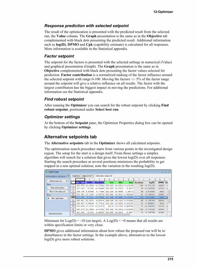
12-Optimizer

215

Response prediction with selected setpoint

The result of the optimization is presented with the predicted result from the selected run, the Value column. The Graph presentation is the same as in the Objective tab complemented with black dots presenting the predicted result. Additional information such as log(D), DPMO and Cpk (capability estimate) is calculated for all responses. More information is available in the Statistical appendix.

Factor setpoint

The setpoint for the factors is presented with the selected settings in numerical (Value) and graphical presentation (Graph). The Graph presentation is the same as in Objective complemented with black dots presenting the factor values selected for prediction. Factor contribution is a normalized ranking of the factor influence around the selected setpoint with range 0-100. Moving the factors +/- 5% of the factor range around the setpoint will give a relative influence on all results. The factor with the largest contribution has the biggest impact in moving the predictions. For additional information see the Statistical appendix.

Find robust setpoint

After running the Optimizer you can search for the robust setpoint by clicking Find robust setpoint, positioned under Select best run.

Optimizer settings

At the bottom of the Setpoint pane, the Optimizer Properties dialog box can be opened by clicking Optimizer settings.

Alternative setpoints tab The Alternative setpoints tab in the Optimizer shows all calculated setpoints.

The optimization search procedure starts from various points in the investigated design region. The setup for the start is a design itself. From those settings a simplex algorithm will search for a solution that gives the lowest log(D) over all responses. Starting the search procedure at several positions minimizes the probability to get trapped in a non optimal solution; note the variation in the resulting log(D).

Minimum for Log(D) = -10 (on target). A Log(D) < =0 means that all results are within specification limits or very close.

DPMO gives additional information about how robust the proposed run will be to disturbances in the factor settings. In the example above, alternatives to the lowest log(D) give more robust solutions.

MODDE 11

216

After convergence, you can always click Run optimizer (play) to restart the optimizer. It restarts from the displayed resulting runs of the previous search. If you do not want to continue with the resulting runs click New start points or New from selected (dialog box below displayed) to specify other start runs.

In the dialog box displayed, the run you marked is the default run to optimize around. To switch to another run, enter another run in the Center around optimizer run box.

Enter the percent of the factor range in the Factor range box. The percentage entered here is used to calculate the new high and low limits for the start runs.

Optimizer Properties

In the Optimizer window, click Optimizer settings to open the Optimizer Properties dialog box.

Settings tab

Feature Description Default

Use absolute response limits

When selected, only the runs where all responses are predicted inside the specified limits are displayed in the list.

Not selected.

Include weight in calculation of Log(D)

When selected, the weight specified in the response spreadsheet is included when calculating Log(D).

Selected.

12-Optimizer

217

Feature Description Default

Factor precision

When selected, the DPMO is calculated for runs where all responses are predicted inside the specified limits. The Precision value for the factors specifies the range used in the DPMO calculations.

This is a sensitivity analysis that indicates if a solution is sensitive or insensitive to small changes in the factor settings.

Selected.

Model error When selected, the probability analysis (DPMO) includes the model error.

Selected.

Simulations The number of simulations in the calculation of the DPMO. The result is scaled up to the unit 'dots per million operations'

10 000

Weight factor contribution

Will give a higher contribution weight to a factor that has a setpoint value which predicts a response close to a defined limit by dividing the factor contribution with the distance to the limit.

Not selected.

Factor contribution range

The part of the factor range used as variation around the setpoint to calculate factor contribution.

5%

Note: If the Factor precision and Model error check boxes are both cleared, no simulations are done. The results then lack probability estimation.

Optimizer Properties, Columns tab

Presents additional columns in the Objective response settings section for the different pages in the Optimizer.

MODDE 11

218

Objective page

In the Weight column you can enter a number between 0.1 and 1 reflecting the importance of the response. Default is 1 indicating that all responses are of equal importance. Individual weights for the responses results in an optimization where the responses with higher weights are favored in the quest for all responses to reach inside the limits.

Note: For the weight change to have the expected result, the selected desirability needs to be Target.

To control the optimization, the overall desirability function, f(ds), plays a key role, as well as reasonable limits and targets for the responses. The optimizer will strive to reach the lowest possible value of the overall desirability function, f(ds), and will strive to reach the lowest possible value. The shape of the function is controlled by the settings of the criteria (Min, Target, Max) for each response and the choice of the dk functions.

With weight 1, the lowest possible value of the individual desirability functions, dk, is -100. Note that in the plots, the individual desirability function, dk, is translated to [-1, 0], so that a weight of 1 has a lowest possible value in the plot of -1, and so on. The goal is to reach a minimum in the overall desirability function, f(ds).

For information about the Desirability column, see the Optimizer desirability section earlier in this chapter.

Setpoint page

The DPMO, Cpk, Cp and k' columns that can be selected for the page all display calculated values that you may want to display.

Alternative setpoints page

The DPMO, Cpk, Cp and k' columns that can be selected for the page all display calculated values that you may want to display.

Optimizer list The Optimizer list shows the setup used by the optimizer and the final results including robust setpoint and hypercube information when available.

12-Optimizer

219

To open the Optimizer list, with the Optimizer as the active window, on the Tools tab, click List.

Optimizer tab After clicking Optimizer on the Predict tab or the Home tab, the Optimizer contextual tab becomes available.

The Optimizer tab contains functions that are related to the Optimizer. These functions, described in this section, are,

Optimizer - to reactivate the Optimizer window,

Dynamic profile,

Contour,

Sweet spot,

Design space,

Design space explorer - Opens the Design Space Explorer dialog box if Find robust setpoint has not been run, otherwise the plot,

Setpoint analysis,

Design space in the Setpoint group, and

Individual response analysis in the Setpoint group.

The Optimizer List is opened by clicking List on the Tools tab.

Note: The Optimizer tab is available only after the optimizer has been run.

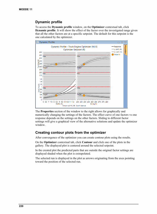
MODDE 11

220

Dynamic profile To access the Dynamic profile window, on the Optimizer contextual tab, click Dynamic profile. It will show the effect of the factor over the investigated range given that all the other factors are at a specific setpoint. The default for this setpoint is the one calculated by the optimizer.

The Properties section of the window to the right allows for graphically and numerically changing the settings of the factors. The effect curve of one factors vs one response depends on the settings on the other factors. Sliding to different factor settings will give a graphical view of the alternative solutions and update the optimizer window.

Creating contour plots from the optimizer After convergence of the optimizer you can create contour plots using the results.

On the Optimizer contextual tab, click Contour and click one of the plots in the gallery. The displayed plot is centered around the selected setpoint.

In the created plot the predicted parts that are outside the original factor settings are displayed shaded when the plot is extrapolated.

The selected run is displayed in the plot as arrows originating from the axes pointing toward the position of the selected run.

12-Optimizer

221

Contour plot wizard from the optimizer After convergence of the optimizer you can create contour plots using the results. On the Optimizer contextual tab, click Contour to open the Factor Setup dialog box.

Select factor settings

In the Factor Setup dialog:

Center around the setpoint found by the optimizer is by default marked, and the run to use in the center is the one you marked. If you want to select another run enter the new run number.

Selecting Factor definitions results in displaying same factor settings as when you enter the contour plot/sweet spot/design space wizard from the Predict tab

Selecting Optimizer factor setup results in displaying the current factor settings in the Optimizer.

Center around the setpoint found by the optimizer

With Center around the setpoint ... selected, clicking OK opens the plot wizard dialog box.

If you create a 2D plot the first two factors are varied around their setpoint settings (20% range) and the other factors are set constant to their setpoint values.

If you create a 4D plot the first two factors are varied around their setpoint settings (20% range), the 3rd and 4th are set at their low, high, and center values using the 20% setpoint range, and other factors are set constant to their setpoint values.

The resulting plot displays the area outside the design factor range shaded.

The selected run is displayed in the plot as arrows originating from the axes pointing toward the position of the selected run.

This option is unavailable for mixture (formulation) factors.

Creating a sweet spot plot from the optimizer When you choose to create the sweet spot plot from the optimizer, MODDE uses the acceptance range of the responses as specified in the optimizer response spreadsheet fields Min, Target, and Max.

To create the sweet spot plot click Sweet spot on the Optimizer contextual tab, and click one of the plots in the gallery. The displayed plot is centered around the selected setpoint.

MODDE 11

222

In the created plot the predicted parts that are outside the original factor settings are displayed shaded when the plot is extrapolated. The selected run is displayed in the plot as arrows originating from the axes pointing toward the position of the selected run.

Sweet spot plot wizard from the optimizer When you choose to create the sweet spot plot from the optimizer, MODDE uses the acceptance range of the responses as specified in the optimizer response spreadsheet fields Min, Target, and Max.

Select factor settings

In the Factor Setup dialog:

Center around the setpoint found by the optimizer is by default marked, and the run to use in the center is the one you marked. If you want to select another run enter the new run number.

Selecting Factor definitions results in displaying same factor settings as when you enter the contour plot/sweet spot/design space wizard from the Predict tab

Selecting Optimizer factor setup results in displaying the current factor settings in the Optimizer.

Center around the setpoint found by the optimizer

With Center around the setpoint ... selected, clicking OK opens the plot wizard dialog box.

If you create a 2D plot the first two factors are varied around their setpoint settings (20% range) and the other factors are set constant to their setpoint values.

If you create a 4D plot the first two factors are varied around their setpoint settings (20% range), the 3rd and 4th are set at their low, high, and center values using the 20% setpoint range, and other factors are set constant to their setpoint values.

The resulting plot displays the area outside the design factor range shaded.

The selected run is displayed in the plot as arrows originating from the axes pointing toward the position of the selected run.

This option is unavailable for mixture (formulation) factors.

12-Optimizer

223

Creating a design space plot from the optimizer After convergence of the optimizer you can create design space plots using the results. The Design Space Plot is based on the result of Monte Carlo simulations done on the models for the responses that are active in the optimizer. The important properties that separate the Design Space Plot from a Sweet spot plot can be found in the Design Space Plot Properties described later in this section.

On the Optimizer contextual tab, click Design space and click one of the plots in the gallery. The displayed plot is centered around the selected setpoint.

In the created plot the predicted parts that are outside the original factor settings are displayed shaded when the plot is extrapolated.

The selected run is displayed in the plot as arrows originating from the axes pointing toward the position of the selected run.

Design space wizard from the optimizer When you choose to create the design space plot from the Optimizer contextual tab, MODDE uses the acceptance range of the responses as specified in the optimizer response spreadsheet fields Min, Target, and Max.

Select factor settings

In the Factor Setup dialog:

Center around the setpoint found by the optimizer is by default marked, and the run to use in the center is the one you marked. If you want to select another run enter the new run number.

Selecting Factor definitions results in displaying same factor settings as when you enter the contour plot/sweet spot/design space wizard from the Predict tab

Selecting Optimizer factor setup results in displaying the current factor settings in the Optimizer.

Center around the setpoint found by the optimizer

With Center around the setpoint ... selected, clicking OK opens the plot wizard dialog box.

If you create a 2D plot the first two factors are varied around their setpoint settings (20% range) and the other factors are set constant to their setpoint values.

If you create a 4D plot the first two factors are varied around their setpoint settings (20% range), the 3rd and 4th are set at their low, high, and center values using the 20% setpoint range, and other factors are set constant to their setpoint values.

MODDE 11

224

The resulting plot displays the area outside the design factor range shaded.

The selected run is displayed in the plot as arrows originating from the axes pointing toward the position of the selected run.

This option is unavailable for mixture (formulation) factors.

Design space plot options

Click Plot options... on the first page in the wizard to open the plot options, alternatively right-click the created plot and click Properties. The Design Space Contour Options lets you specify,

Resolution - A higher resolution means a more detailed plot, but it can also slow down your computer.

Use color - This determines if the plot should be colored or merely display the contour lines.

Show contour level labels - Select to display contour level labels.

Output - Choose between Probability of failure (%) and Probability of failure (DPMO). Probability of failure (%) is default selected.

Limit - The acceptance criteria to aim for either in percentage or in the DPMO space.

Simulations/point - The number of simulations per point; the higher the more time consuming but also more accurate.

Include model error - This determines if model error should be included in the plot. Note that when this check box is cleared, the plot merely presents the same information as the Sweet spot plot.

Interval type, Confidence level and Tolerance proportion on the Interval estimation tab. For more, see the Interval type and probability levels subsection in chapter 4, File.

12-Optimizer

225

Find robust setpoint After running the Optimizer you can search for the robust setpoint. The robust setpoint function will maximize the distance from the acceptance boundaries in the Design Space. The procedure will be to first generate the design space with selected factors and a given specification. It can be very time-consuming, depending on the settings chosen. The resolution must be considered when you search for the robust setpoint; it is very easy to get an overly large data set that takes a long time to calculate. Note that the dialog box tells you how many points are going to be simulated based on the number of factors selected and your resolution. The greater the resolution, the tighter the grid of points that are calculated.

The number of points and calculations:

Number of points to be simulated = number of responses * (resolution^(number of selected factors)).

Number of calculations = number of responses * (resolution^(number of selected factors)) * Iterations.

To search for the robust setpoint;

1. In the Optimizer window, click Find robust setpoint or on the Optimizer contextual tab, click Design space explorer. When you click Design space explorer the plot automatically opens when the calculations are complete.

2. Select which factors to use, the resolution, iterations, DPMO limit, and if model error and factor precision should be included.

3. Optionally change Interval estimation settings on the Interval estimation tab.

4. When you are happy with your settings and the number of points to be simulated, click OK.

MODDE 11

226

Robust setpoint results

If a robust setpoint was found, the result is added to the optimizer Alternative setpoints list as a run with the notation R. The factor settings are shown in the Setpoint tab and the corresponding result is shown in the response spreadsheet. This point is also displayed as a cross with arrows pointing to the robust setpoint, in the Design Space Explorer plot automatically opened after completing the calculations.

Detailed information is presented in the Optimizer List.

Robust low/high edge: The setting of the factor that reaches the low/high boundary of the Design Space as a Manhattan distance (perpendicular distance in the factor space) from the robust point to the Design Space limit.

Robust resolution distance: The calculations of the robust point are done with a specific resolution. The resolution limits the position of the robust setpoint. If the robust distance is less than 4 the recommendation is to increase the resolution for the robust setpoint estimate. The Robust low edge and Robust high edge are calculated from those resolution values and define the robust range.

Hypercube low edge and Hypercube high edge: The factor settings that define the design space hypercube.

Relative volume: The relative volume in Design Space calculation is the resolution^number of factors, in this case 32^3 = 32 768. The part of this volume that is considered as a DS count = 1764; the DS count corresponding to Relative volume = 5.38%.

12-Optimizer

227

Design space explorer

The Design Space Explorer allows you to investigate the Design Space volume by sliding the constant factors to alternative settings.

To display the Design Space Explorer plot the calculations, specified in the Find Robust Setpoint dialog, have to be performed. This dialog opens when clicking Design space explorer on the Optimizer tab or Find robust setpoint in the Optimizer window Setpoint tab.

If a robust setpoint is found, that point is displayed in the Design Space Explorer plot as arrows forming a cross pointing to it. The setting for the factors held constant is also marked with an arrow along the slider in the Properties pane.

The dotted frame in the Design Space Explorer plot designates the largest possible regular hypercube that can be inserted into the irregular design space volume. How this regular hypercube extends into many dimensions is given by the green bars seen in the Hypercube range part in the picture above. The green bars mark the mutual ranges within which all factors can be changed at the same time and without further restrictions.

Note: When sliding a constant factor, the arrows at the end of the lines disappear but the lines are still displayed to show where the setpoint was. The arrows reappear when all constants are at their respective setpoint again.

Hint: You can move the current setpoint by right-clicking the new position in the plot and clicking Set as selected setpoint. This new point can then be evaluated using Setpoint analysis. Note here that the original robust setpoint cannot be displayed after selecting a new setpoint in the plot without full recalculation.

To save the calculated results from search for the robust setpoint;

1. Create the Design Space Explorer plot.

2. On the Tools tab, in the Create group, click List and then save that list.

Displayed in the list are the coordinates for the factors and the overall DPMO for the included responses.

MODDE 11

228

Setpoint analysis

Using setpoint analysis we can show how the factor settings can be varied around a selected setpoint and still fulfill the response criteria that correspond to the factor tolerance that can be used at the setpoint.

Limitations with a sweet spot or design space plot presentation are the number of dimensions and the lack of probability estimate in the predicted surface (Sweet spot plot only). Setpoint analysis uses the setpoint that was selected in the Optimizer (either the optimal point or the robust point). From there it increases the variation for the respective factors until it has reached the limit of predicted distribution for the responses. These calculations have to consider both the definition limits for the responses as well as the DPMO accepted value.

The estimation is performed using Monte Carlo simulations on the factor settings. MODDE performs a search to identify the largest possible tolerance range for each factor that can be used and still meet all response requirements. The default limit is less than 10 000 (1%) hits outside the limits for each response. The results are displayed in the Setpoint Analysis window.

To open the Setpoint Analysis window,

1. On the Predict tab or Home tab, click Optimizer.

2. Run the Optimzer.

3. Then on the Optimizer contextual tab, click Setpoint analysis.

For more information about the Setpoint Analysis window, see Chapter 13, Setpoint.

229

13-Setpoint

Introduction Using setpoint analysis we can show how the factor settings can be varied around a selected setpoint and still fulfill the response criteria that correspond to the factor tolerance that can be used at the setpoint.

Limitations with a sweet spot or design space plot presentation are the number of dimensions and the lack of probability estimate in the predicted surface (Sweet spot plot only). Setpoint analysis uses the setpoint that was selected in the Optimizer (either the optimal point or the robust point). From there it increases the variation for the respective factors until it has reached the limit of predicted distribution for the responses. These calculations have to consider both the definition limits for the responses as well as the DPMO accepted value.

The estimation is performed using Monte Carlo simulations on the factor settings. MODDE performs a search to identify the largest possible tolerance range for each factor that can be used and still meet all response requirements. The default limit is less than 10 000 (1%) hits outside the limits for each response. The results are displayed in the Setpoint Analysis window.

Setpoint analysis plots and lists To open the Setpoint Analysis window,

1. On the Predict tab or Home tab, click Optimizer.

2. Run the Optimzer.

3. Then on the Optimizer contextual tab, click Setpoint analysis.

After opening the Setpoint analysis window, the following Setpoint analysis features are available;

Factor distribution

Response distribution

Individual response analysis

Design space contour plot

Setpoint summary.

MODDE 11

230

Setpoint window The Setpoint Validation and Setpoint Analysis windows function in the same way. The windows consist of a factor and a response spreadsheet.

The Setpoint Analysis window appears when clicking Setpoint analysis on the Optimizer contextual tab.

The Setpoint Validation window appears when clicking Setpoint validation on the Predict tab. In the validation case, the preset conditions used are the factor average and the full range as input for the prediction.

For factors, the yellow Setpoint lines and the blue distribution range can be changed by using the mouse pointer to click and drag or by typing new values in the fields. The red lines are the normalized design specification lines.

For responses, the yellow Target lines and the red Max/Min lines can be moved either by typing a new value in the appropriate fields or by using the mouse pointer to click and drag the lines to the desired levels.

Every change in settings is followed by a recalculation by default. This might be disturbing when tuning several settings, so it is possible to turn off automatic recalculation preventing the automatic update.

Preventing auto update To prevent the Setpoint window from automatically updating on every change,

1. Right-click the Setpoint window.

2. Click Properties.

3. Clear the Automatic update check box.

With automatic updating turned off, you will need to click Click to resample under Predicted response profile.

Adding more columns You can add more columns to the Factor and Response spreadsheets in the Setpoint window;

1. Right-click the header row in the Response/Factor spreadsheet.

2. Select and clear as desired.

3. To restore, click Restore default layout.

Setpoint properties Right-click the Setpoint validation or Setpoint analysis window to open the Properties dialog box.

13-Setpoint

231

Parameters section

In the Parameters section, the settings used in the setpoint analysis/validation are displayed and can be adjusted.

Option Description Default

Acceptable range simulations

Number of simulations done in each step of the search for the acceptable range for the factors.

20 000

Response profile simulations

Number of simulations for the final predictions of the response profile.

50 000

DPMO limit Defects Per Million Opportunities outside the specification limits. The first response that exceeds this limit will stop the expansion of the accepted factor range.

10 000

Use total DPMO Stop criterion will be the total number of predictions outside the limit for all responses. When not selected the DPMO limit is for each response.

Not selected.

Include model error Includes model error in the predictions of the response distribution.

Selected.

Automatic update

Any change in the settings results in a recalculation of the Setpoint analysis/validation.

Clear this check box to do the calculations when all settings have been adjusted instead of after each adjustment.

Selected.

Limits at 95 or 99 % confidence for

Defines the Low and High values in such a way that 95%, in the default case, of the Monte Carlo simulations

95%

MODDE 11

232

Option Description Default

normal distribution are inside the limits. Selecting 99% widens the included area by lowering the Low limit and increasing the High limit in the factor spreadsheet.

Show and Color range sections

In the Show and Color range sections, to display limits and colors of the graphs can be specified.

Option Description Default

Possible Min/Max lines

Display the possible minimum and maximum for the factors, as listed on the Objective page in the Optimizer.

Not selected.

Color range Displays the range of colors of the distribution bars.

Blue for factors, green for responses.

Note: You can select which columns to display for the Factor and Response spreadsheets respectively by right-clicking the header row in the Setpoint window.

Factor spreadsheet

In the factor spreadsheet the following functionality is available for each factor;

Item Description Default

Low, Setpoint, High. The acceptable factor range

The largest range that complies with the response criteria, estimated by MODDE.

Std. dev. One standard deviation of the used factor range.

Calculated.

Role

Free: The largest possible range of variation for the specific factor is used, with respect to the settings for other factors and response specifications.

Locked: The range settings of the factor are locked according to the set range.

For Setpoint validation: by default 'Locked'.

For Setpoint analysis: by default 'Free'.

Distribution

The distribution to be used for each factor range.

Uniform: All factor settings within the specified range have the same probability to appear.

Normal: The simulations are normally distributed within the factor range.

Triangular: The distribution has the shape of a triangle; a good way to get a skewed distribution for a factor.

Target: The factor is set to a fixed value, the setpoint value.

For quantitative factors, by default 'Normal'.

For formulation factors, by default 'Triangular'.

Possible min

The left side of the T bar in the Estimated acceptable range is the estimated minimum factor value for which the predictions still fall inside the specifications when all other factors are locked at the setpoint.

Calculated, by default not shown.

13-Setpoint

233

Item Description Default

Possible max

The right side of the T bar in the Estimated acceptable range is the estimated maximum factor value for which the predictions still fall inside the specifications when all other factors are locked at the setpoint.

Calculated, by default not shown.

Estimated acceptable range

The yellow lines are the default factor settings of the selected run in the optimizer.

The red lines are the Low and High factor settings of the experimental region.

The blue region represents the 95%* part of random factor variability with normal distribution where all predictions are within the specifications.

Not default displayed: The black T bar represents the region of acceptable variability valid for that factor when all other factors are locked at the setpoint. Valid means that all predictions of the responses are within the specifications. No model error is considered in this search.

*95% is the default. In Setpoint Properties you can change it to 99%.

Response spreadsheet In the response spreadsheet the following functionality is available for each response:

Item Description Default

Min, Target, Max

The optimization range Min, Target, and Max as specified in the Optimizer.

Criterion What the algorithm is aiming for.

Minimize, Maximize, Target, and Predicted as specified in the optimizer. The criterion Not met signifies that the response was excluded from the calculations.

Cpk

A Process Capability Index, Cpk, which originates from the Six Sigma statistics, is estimated in this simulation. Cpk = 1 means that approximately 0.13%* of the predictions will fall outside the specifications.

Not displayed.

Estimated by MODDE when selected.

Cp

The process potential index, Cp, estimates what a process is “capable” of producing if the target is centered between the specification limits under the “natural” tolerance 6σ. If Cp = 1, the process is said to be “capable”. Originates from the Six Sigma statistics.

Not displayed.

Estimated by MODDE when selected.

k'

The process deviation index, k, estimates the amount of deviation of the process mean from the target. Originates from the Six Sigma statistics.

Not displayed.

Estimated by MODDE when selected.

DPMO

Defects Per Million Opportunities is an estimate of how many predictions will be outside the specification per one million predictions in the setpoint analysis/validation with the selected distribution.

Estimated by MODDE.

MODDE 11

234

Item Description Default

Average The average of the predicted response values.

Not displayed.

Calculated by MODDE when selected.

Std. dev. The standard deviation of the predicted response values.

Not displayed.

Calculated by MODDE when selected.

% outside Percentage of predicted points found outside the Min and Max limits.

Not displayed.

Estimated by MODDE when selected.

Median The median of the predicted response values.

Not displayed.

Calculated by MODDE when selected.

1st quartile 25% of the predicted response values are found below this value.

Not displayed.

Calculated by MODDE when selected.

3rd quartile 25% of the predicted response values are found above this value.

Not displayed.

Calculated by MODDE when selected.

Predicted response profile

The yellow line represents the Target value for the response as specified in the Optimizer.

The red lines are the specification limits for each response as specified in Optimizer.

The faded green region represents the predictions for a random distribution of factor settings in the given ranges (low-setpoint-high).

* See the table in the DPMO and process capability indices subsection in the Statistical appendix.

Factor distribution Open the Predictive Factor Distribution Plot by clicking the histogram to the far right on each row .

This histogram displays the distribution of the factor settings used for the simulation. The specified Min and Max values are displayed as lines.

Hint: You can also display the Predictive Factor Distribution Plot by double-clicking Estimated acceptable range.

13-Setpoint

235

Response distribution To display the result of the Monte Carlo simulations as frequency histograms, on the Setpoint analysis or Setpoint validation window, click the histogram Open

predicted response distribution plot to the far right .

Hint: You can also display the Predicted Response Distribution Plot by double-clicking Predicted response profile.

Setpoint summary The Setpoint Summary list shows the information displayed in the Setpoint analysis or Setpoint validation window.

To open the Setpoint Summary list, with the Setpoint analysis/validation as the active window, on the Tools tab, click List.

Individual response analysis To open the Individual Response Analysis window, on the Optimizer contextual tab, click Individual response analysis.

The window shows the acceptable factor ranges for specific responses.

MODDE 11

236

Setpoint, design space In the Setpoint analysis group on the Optimizer contextual tab, click Design space to open the Design Space Plot wizard.

This plot can be investigated from two angles:

1. Visualization of the 2D design space from any selected setpoint - here the Include distribution from setpoint analysis on axis factors check box should be cleared while the Include distribution from setpoint analysis on constant factors check box should be selected.

2. Analyze the size and shape of the design space at any given setpoint with a specific factor tolerance - here both check boxes should be selected.

Click Finish to see the Design Space Plot showing the probability of failure (%) for the shown factor combinations. Alternatively, Next to specify the settings for the constant factors.

237

14-Report

Introduction MODDE has an automatic report generator. In the report, basic formatting functionality is available for writing text. Plots, lists, and model results of MODDE can be added to the report at any time. These items are added to the report as placeholders. A placeholder stands in the place of contents which MODDE will provide, let it be a plot, list or any text or number. The placeholders enable you to save the report as a template and use it for different investigations.

Opening the Report generator To create a new report, on the File tab, click Info and then click Report. A dialog box opens and you can select which template to open.

If you have saved a report with the investigation, MODDE automatically opens that report.

Hint: You can also open the report by pressing Ctrl+R, adding the current window to the saved/blank report.

MODDE 11

238

When your investigation has not been fitted MODDE will ask to fit the investigation so it can automatically fill all the placeholders.

Saving a report To save a report created in this version of MODDE, save and close the investigation. The report is automatically saved with the .mip.

To save a report created in MODDE 10 or earlier, see the Opening and saving an old report subsection next.

To save the report as a separate file, on the File tab, click Save as, and then click Save a copy.

Note that this separate file is NOT saved with the investigation, but only as a separate copy of the report. However, if you then click Save in the report and also Save in the MODDE window, the current report is also saved with the .mip.

Opening and saving an old report To open a report saved in MODDE 10 or earlier,

On the File tab, click Info and then click Report. In the Select Templates dialog, browse for the old report.

Or,

If a report was already saved with the investigation, in the report generator click Open on the File tab and browse for the old report.

To save the old report,

With the investigation it was opened for, on the File tab, click Save.

Or,

Separately to file, on the File tab, click Save as | Save a copy.

Note that this separate file is NOT saved with the investigation, but only as a separate copy of the report. However, if you then click Save in the report and also Save in the MODDE window, the current report is also saved with the .mip.

14-Report

239

Report window The Report window contains:

File tab, containing overall commands such as New and Open but also Template commands.

Home tab, containing all commonly used commands including clipboard, formatting, alignment etc.

View tab, containing placeholder commands, views and panes.

Quick Access Toolbar, by default containing Save, Undo, Redo and Customize. Customize allows you to select how to display the ribbon and which of the following commands to display: New, Open, Save, Save as, Print, Print preview, Undo, Redo.

Main window, showing the report template.

File tab On the File tab you find the general Windows commands and additional MODDE specific commands; New, Open, Save, Save as, Templates, Print, Exit, and Recent templates.

General Windows commands Click New to create a new report from the selected template.

Click Open to open a report or template saved in MHT or HTML format.

Click Save to save the report with the current investigation.

Click Print to Print the report, open the Page setup dialog, or Print preview to preview the report.

Click Exit to close the report.

MODDE 11

240

Save as Click File | Save as |

Save a copy to save the report as a separate file in MHT or HTML format.

Note that this separate file is NOT saved with the investigation, but only as a separate copy of the report. However, if you then click Save in the report and also Save in the MODDE window, the current report is also saved with the .mip.

Save as template to save the current template when you have changed/created a template according to your wishes and want to save it to use it as template when you generate a report.

You can save and copy custom templates by clicking Templates on the File tab.

Templates

Click Templates |

Copy templates to search for templates to copy to the templates folder making them available in the Select templates dialog box when creating a new report.

Templates folder to view the available custom templates, delete or copy.

Note: The default templates MKS Umetrics default and Blank cannot be modified nor deleted.

Recent templates

Under Recent templates, the templates used to create a new report are listed.

Home

Introduction On the Home tab you find the most commonly used commands, organized in groups: Clipboard, Font, Paragraph, Insert, Editing, and Report.

14-Report

241

Clipboard In the Clipboard group you find the standard commands

Paste (Ctrl+V)

Paste | Paste unformatted (Ctrl+Shift+V)

Cut (Ctrl+X)

Copy (Ctrl+C)

To clear the marked content, press the Del key.

Undo (Ctrl+Z) and Redo (Ctrl+Y) are available in the Quick Access Toolbar.

Font and Paragraph For details about the Font and Paragraph groups, see the Formatting topic.

Insert Use the Insert group to insert a Picture, Template, or File into the current report.

Picture

Click Picture to insert a picture in the report. You can also right-click the report and then click Insert picture.

Template

Click Template to open a dialog box where you can select a custom template to insert in the report. To be able to select the template it must be available in the templates folder. Templates can be added manually or by using the File | Save as | Save as template or File | Templates | Copy template commands.

File

Click File to insert a web page file (*.htm, *.html), text file (*.txt), or picture file (*.jpg, *.png, *.gif, *.bmp).

Editing

In the Editing group you find the standard commands

Find (Ctrl+F)

Select all (Ctrl+A)

Report The Report group contains commands for updating all placeholders, viewing the report in a browser and editing the report in the editor of your choice.

MODDE 11

242

Update report

Click Update report to update all placeholders to the default plots and lists of the current investigation.

Note that any customization, not saved in the currently used plot template, will be lost when clicking Update report. For instance, if you have enlarged/colored one point in a scatter plot and added it to the report, clicking Update report will result in the default plot, without that customization.

To keep the visualization of a plot, with customizations, remove the placeholder for that particular plot by clicking it so that it becomes selected and on the View tab clicking Update placeholder.

Open with

Click Open with to view or edit the current report. You can continue to work with your report in the editor of your choice by selecting an editor. The applications listed here are the installed applications that have registered that they can view or edit HTML text with Windows.

Formatting In the Font group the standard commands, such as text style, font, font size, bold, italic, underline, strikeout, highlight color, and text color, are available. The two last commands are:

Convert to hyperlink - Converts the current marking to a hyperlink after selecting hyperlink type and url.

Styles - Opens the Styles and Formatting dialog for customization and preview of the text styles in the report.

In the Paragraph group, indenting, numbering, bullets, aligning and show formatting are available.

View tab On the View tab you can select to hide or show the following:

Document views

Editing view - regular report with placeholders filled with content.

Template view - report displaying placeholders.

14-Report

243

Placeholders

Remove all placeholders - removes all placeholders in the report leaving static plots, lists and details.

Update placeholder - updates the selected placeholder.

Show placeholder - shows the selected placeholder.

Remove placeholder - removes the selected placeholder.

Placeholders - displays/hides the Placeholders window holding all placeholders that can be added to the report.

Properties - displays/hides the properties of plots and images that can be customized. The Properties window also displays the default settings for plots.

Placeholders window Open the Placeholders window by selecting the Placeholders check box on the View tab.

The combo box lists different categories of placeholders.

MODDE 11

244

To insert a placeholder in the report, mark the placeholder and click Insert, alternatively double-click the placeholder. The newly inserted placeholder is automatically updated.

To show the underlying placeholders, on the View tab, click Template view.

Properties window Open the Properties window by selecting the Properties check box on the View tab.

In the Properties window you can change the default plot size and to save a plot as .png, .bmp, .jpg or .emf (.emf for 2D only).

Properties for placeholders are displayed when you click the placeholder. You can change the properties of the current placeholder in the Placeholder settings section in the properties window. The Default settings section displays and allows changing of the default placeholder properties.

Note: For changes in Default settings to take effect the report has to be updated (Update report), reverting all plots and lists to the default for the current investigation. See also the Update report subsection earlier in this chapter.

Adding plots and lists to the report To add a plot or list to the report;

1. Click the desired position in the report so that the pointer is where the plot or list should be placed.

2. Right-click the plot or list in MODDE.

3. Click Add to report.

Hint: You can press Ctrl+R in MODDE to place the currently selected plot or list into the current location in the report.

245

Statistical appendix

Introduction The statistical appendix gives a more detailed, mathematical and statistical look into the calculations used in MODDE.

Fit methods MODDE currently supports two regression methods for fitting a model to the data. These are multiple linear regression (MLR) and partial least squares regression (PLS or PLS regression). Both models predict one (or several) dependent variables, Y (n × m), also called the responses, by a regression model from a set of independent variables, X (n×p), also called the factors, such that

Y = XB + E,

where B is a p×m vector of regression coefficients and E is a matrix of residuals. The prediction of the dependent variables is

Ŷ = XB.

The column dimension, p, in the data matrix, X, denotes the number of terms in the model, and includes the intercept.

Multiple linear regression (MLR) Multiple linear regression (MLR) is extensively described in the literature, and this section will only identify the numerical algorithm used to compute the regression coefficients. For additional information on MLR, see e.g. Draper and Smith (1981).

The MLR model relates a set of dependent variables, Y (n×m), also called the responses, by a linear regression model to a set of independent variables, X (n×p), also called the factors, such that

Y = XB + E,

where B is a p×m vector of regression coefficients and E is a matrix of residuals. The prediction of the dependent variables is

Ŷ = XB.

In MLR, the regression can be posed as an optimization problem

MODDE 11

246

MLR thus minimizes the squared difference between the dependent variables, Y, and the linear prediction model, XB. MODDE uses the singular value decomposition (SVD) to obtain the regression coefficients; see Golub and Van Loan (1983) for a description of the SVD and its use to obtain the regression coefficients.

Note: In case of missing data in a row, the row is excluded for the relevant response before the MLR model is fit.

References

Draper, Norman and Smith, Harry, Applied Regression Analysis, Second Edition, Wiley, New York, 1981.

Golub, Gene H. and Van Loan, Charles F, Matrix Computations, The Johns Hopkins University Press, Baltimore, 1983.

Partial least squares regression (PLS) When the problem is poorly conditioned, the variables are correlated or p > n, regularization is needed in order to stabilize the model and to avoid overfitting. PLS regression is a latent variable method that offers regularization by representing the dependent variables by a small set of linear combinations (the latent variables) of the variables, and by that reducing the dimension of the space spanned by the independent variables. PLS also offers improved interpretation of the regression model.

PLS regression is described extensively in the existing literature, which is why only a brief description will be given here.

PLS1

In the case when m = 1, PLS solves the same loss function as MLR, but with a constraint on the regression coefficients. This problem is sometimes called PLS1. The optimization problem is posed as

where

is a Krylov subspace generated by X'X and X'y, and where A is the number of components of the PLS regression model.

PLS regression is a non-linear regression method, because the dependent variable, y, is included in the prediction model.

Note: When the models for the responses are different, PLS regression fits each response separately.

PLS2

The case when m > 1 is sometimes called PLS2. The PLS regression model relates a set of dependent variables, Y (n × m), also called the responses, by a regression model to a set of independent variables, X (n × p), also called the factors, such that

Y = XB + E,

where B is a p×m vector of regression coefficients and E is a matrix of residuals. The prediction of the dependent variables is

Ŷ = XB.

Statistical appendix

247

The PLS regression algorithm creates new variables, ta, called X scores, as linear combinations of the original variables, i.e., such that ta = Xwa, where wa is a vector of weights. These X scores are few, often just two or three, and orthogonal. The X scores are then used to model the responses.

With more than one response, i.e., when m > 1, the Y variables are similarly combined to a few Y scores, ua, by using weights, ca, such that ua = Yca.

The PLS regression model finds the score vectors by solving the optimization problem

for a = 1, 2, …, A, such that all Xawa and Xbwb for a ≠ b are orthogonal. The orthogonality is enforced by deflating the found variation from the X and Y matrices after each component such that

Xa+1 = Xa - tap'a,

Ya+1 = Ya - tac'a,

where pa = X'ata / (t'ata) are called loadings and X1 = X.

The PLS2, the multi-Y problem is less well understood compared to the single-y problem, but nevertheless performs impressively when p > n.

One PLS regression component, indexed by a, consists of one vector of X scores, ta, and one of Y scores, ua, together with the X and Y weights, wa and ca. The scores are collected such that T = [t1, t2, …, tA] and U = [u1, u2, … ,uA], and the loadings P = [p1, p2, … ,pA]. The PLS regression model finally regresses U on T. The final PLS regression model is stated as

X = TP' + E,

Y = TC' + F.

The regression coefficient vector is computed as

B=W(P'W)-1C',

and predictions are made as

Ŷ = XB

A geometric interpretation of the PLS regression method is that it projects the X and Y matrices on lower-dimensional hyper planes, spanned by wa and ca, for a = 1, 2, … , A, respectively, and that the coordinates in this subspace are T and U, that summarize X and Y, respectively, and that the regression model relates T to U.

The matrices X and Y can be seen as n points in two Euclidean vector spaces (in and ), respectively (see the figure below) the X space with p coordinates, and the Y space with m coordinates, p and m being the number of columns in X (terms in the model) and in Y (responses).

MODDE 11

248

The number of components, A, is determined by a cross-validation procedure, in which the prediction error sum of squares (PRESS) is minimized. When A = rank(X), the regression coefficients of PLS regression are equivalent to those of MLR, and hence MLR could be considered as a special case of PLS regression. That is, if you with PLS regression extract all components, the PLS regression model is equivalent to the MLR model.

Cross-validation significance rules In order to determine if a component is significant, MODDE considers the following rules in order:

A component is considered non-significant by Rule 3 if:

A + 1 > min(n,p).

A component is considered significant by Rule 1 if

Q2 > CVlim

or otherwise significant by Rule 2 if

for any k = 1, ... , m.

A component is considered non-significant by Rule 4, regardless of Rule 1 and Rule 2, if

and

for all k = 1, ... , m, and if was not deemed non-significant by Rule 3.

If no rule at all has come in effect yet, the component is considered non-significant by Rule 5.

Statistical appendix

249

The cross-validation limit for Q2, i.e., CVlim, is defined as

MODDE will try to compute at least two PLS regression components (if there exist two), regardless of their significance according to these rules.

Singular models

A model is considered singular if the condition number of X is greater than 3000. Such models may only be fit by PLS regression.

Model

You may edit the model and add or delete terms for individual factors. You may add up to third order terms (i.e., cubic terms, and 3-factor interactions).

In order to regularize a design that is singular with respect to your model, MODDE will fit a PLS regression model to the data. MLR will not be available in this situation.

Hierarchy MODDE enforces a hierarchy of model terms, where simpler terms are higher in the hierarchy. You cannot delete the constant term, it is at the top of the hierarchy. A linear term can only be deleted if the second and third order terms involving the factor have been removed first.

Scaling

Scaling the factor matrix, X When the model is fit with multiple linear regression, the design matrix, X , is scaled and centered by the method specified in the Factor Definition dialog box, in the Advanced tab, by changing the value in the MLR scaling box. The default scaling for MLR is Orthogonal scaling.

When the model is fit with PLS regression, the design matrix, X, is always scaled by Unit variance scaling (see below).

If needed, the scaled design matrix, X, is extended with higher order terms, such as squares, cubes and interaction terms, according to the selected model.

The available scaling choices are:

Orthogonal scaling, where

zij = (xij - Mj)/Rj

in which zj denotes a scaled factor and xj denotes the original factor, Mj is the mid-range of the factor and Rj the range. Mj and Rj are computed as

Mid-range scaling, where

zij = (xij - Mj)

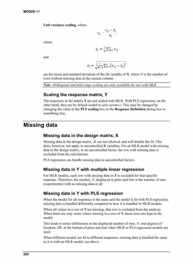
MODDE 11

250

Unit variance scaling, where

where

and

are the mean and standard deviation of the jth variable of X, where N is the number of rows without missing data in the current column.

Note: Orthogonal and mid-range scaling are only available for use with MLR.

Scaling the response matrix, Y The responses in the matrix Y are not scaled with MLR. With PLS regression, on the other hand, they are by default scaled to unit variance. This may be changed by changing the value in the PLS scaling box in the Response Definition dialog box to something else.

Missing data

Missing data in the design matrix, X Missing data in the design matrix, X, are not allowed, and will disable the fit. This does, however, not apply to uncontrolled X variables. For an MLR model with missing data in the design matrix, in an uncontrolled factor, the row with missing data is excluded from the calculations.

PLS regression can handle missing data in uncontrolled factors.

Missing data in Y with multiple linear regression For MLR models, each row with missing data in Y is excluded for that specific response. Therefore, the number, N, displayed in plots and lists is the number of runs (experiments) with no missing data at all.

Missing data in Y with PLS regression When the model for all responses is the same and the model is fit with PLS regression, missing data is handled differently compared to how it is handled in MLR models.

When all values in a row of Y are missing, that row is excluded from the analysis. When there are only some values missing in a row of Y, those rows are kept in the model.

This leads to minor differences in the displayed number of runs, N, and degrees of freedom, DF, at the bottom of plots and lists when MLR or PLS regression models are used.

When different models are fit to different responses, missing data is handled the same as it is with an MLR model, see above.

Statistical appendix

251

Number of observations The number of observations (experiments), N, as used in ANOVA and for the computation of the adjusted R2, is the actual number of non-missing observations for each response column. This value of N and the degrees of freedom, DF = N - p, are displayed at the bottom of ANOVA plots and lists, and on all residual plots (including plots of observed vs. predicted Y).

Summary of fit

R2 The first bar in the Summary of fit plot is the R2, which is the fraction of the variation of the response explained by the model, i.e.

where SSres is the sum of squares of the residual, corrected for the mean and SStot is the total sum of squares of Y corrected for the mean.

Note that the R2 overestimates the goodness of fit.

The R2 value is always between 0 and 1. A value close to 1 indicates that the model fit the data very closely.

R2 Adjusted is the fraction of variation of the response explained by the model, but adjusted for the degrees of freedom of the model, i.e.

where DFtot = n - 1 is the degrees of freedom of the population variance of the dependent variable and DFres is the degrees of freedom of the estimate of the population error variance.

Q2 The second bar in the Summary of fit plot is Q2. The Q2 estimates the predictive ability of the model (also known as model predictive power), i.e., its ability to generalize to new, unseen data. The Q2 is either computed in closed form as in generalized cross-validation or computed in a cross validation-like procedure and is expressed in the same units as R2. The Q2 is defined as

where PRESS is the prediction residual sum of squares, which differs for MLR and PLS regression models, SStot is the total sum of squares of Y corrected for the mean and

is the mean response. See the Measures of goodness-of-fit subsection later in this chapter for more details about Q2.

MODDE 11

252

The Q2 is less than or equal to 1, and a value greater than zero indicates that the model is significant (it performs better than just predicting the mean value, , for each response).

If the regression model is a PLS model, negative Q2 values are set to zero, for computational purposes.

Model validity The third bar in the Summary of fit plot is the Model Validity. When the model validity column is larger than 0.25, the model has no lack-of-fit. This means that the model error is not significantly larger than the pure error.

When the model validity is less than 0.25 there is a significant lack-of-fit and the model error is significantly larger than the pure error (poor reproducibility).

The model validity is computed as

Validity = 1 + 0.57647 log10(plof),

where plof is the p-value for the lack-of-fit test and the value 0.57647 is selected such that plof ≥ 0.05 gives Validity ≥ 0.25.

Reproducibility The fourth bar in the Summary of fit plot is the Reproducibility, which is the variation of the response (often at the center points) under the same conditions as the total variation of the response. It is computed as

Reproducibility = 1 - MSpe/MStot,

where MSpe is the mean square of the pure error and MStot the total mean square of Y.

A reproducibility of 1 signifies perfect reproducibility.

Residual standard deviation (RSD) If the model is a PLS regression model, and it is the same for all responses, the residual standard deviation is computed by using the total number of observations (experiments, runs), i.e., without excluding the rows with missing values. This is displayed in the summary table and at the bottom of all plots and lists, including the ANOVA.

For MLR and PLS regression with different models for the responses, the residual standard deviation is instead computed by using the number of experiments without missing values for each response.

This residual standard deviation is used in interval estimation, for coefficients and in predictions.

Analysis of variance, ANOVA Analysis of variance (ANOVA) decomposes the total sum of squares of a selected response (sum of squares corrected for the mean) into a part due to the regression model and a part due to the residuals. I.e., such that

SStot = SSreg + SSres.

Statistical appendix

253

With corresponding decomposition of the degrees of freedom as

DFtot = DFreg + DFres.

If there are replicated experiments (observations, runs), the residual sum of squares can be further decomposed in a part due for the pure error and one part due to the lack-of-fit of the model, i.e. such that

SSres = SSpe + SSlof.

where the degrees of freedom is decomposed as

where nk is the number of replicates in the kth set of replicates. Note that rows with missing values have been excluded.

Note: DFlof (degrees of freedom for lack of fit) is the same as RDF (real degrees of freedom).

A goodness-of-fit test is performed by an F-test between the lack-of-fit and pure error sum of squares. The test statistic is

which has an F-distribution with the corresponding number of degrees of freedom.

Two ANOVA plots are displayed:

The regression goodness-of-fit test.

The goodness-of-fit test of the lack-of-fit.

Identifying replicates

MODDE checks the rows of the worksheet for replicates. Rows in the worksheet are considered replicates if they match all factor values plus or minus a small tolerance. The default tolerance is 10 % of half the range of a factor, but it can be altered in the MODDE options page, in the File | Options dialog box.

Measures of goodness-of-fit MODDE computes and displays the following statistics:

Q2

The regression models are validated by the Q2 (sometimes also called q2, , or

in the literature). The Q2 estimates the predictive ability of the model, i.e., its ability to generalize to new, unseen data. The Q2 is defined as

where

MODDE 11

254

is the sum of squares of the training samples around the mean (proportional to the variance of the response) and

is the mean response.

When the regression model is an MLR model, the "PRESS" is computed as in generalized cross-validation (see e.g., Golub et al. (1979)), i.e., by

where the predictions ŷi are computed from a model of all samples.

When the model is a PLS regression model, the PRESS is computed in a cross-validation procedure. The cross-validation procedure keeps a part of the data (e.g., 1/Kth of the samples) out of the model and predicts the left-out samples from a model of the kept samples (i.e., the rest of the (K - 1)/K samples). In this case the PRESS is computed as

where is the predicted left-out response values from the cross-validation procedure.

For PLS regression models, the Q2 is computed both for all responses and such that a

is computed for each individual response, j = 1,2,…,m.

A computed Q2 value greater than zero indicates that the model is significant (it performs better than just predicting the mean value for each response). A high Q2, e.g., Q2 > 0.5 indicates that the model has good predictive ability and will have only a small prediction error on new samples. The Q2 is considered large if Q2 > 0.7.

References

Golub, Gene H.; Heath, Michael and Wahba, Grace. Generalized Cross-Validation as a Method for Choosing a Good Ridge Parameter. Technometrics, 21 (2), 1979.

R2 The regression models are also validated by the R2, the coefficient of determination (also sometimes called the multiple correlation coefficient). The R2 denotes the fraction of the response that is explained by the model and is defined as

where the predicted values, ŷi, are computed from a model of all samples.

The R2 could be considered an upper bound on the estimate for how well the model predicts outcomes of new experiments.

Adjusted R2 The adjusted R2 is the fraction of variance of the response explained by the model, but adjusted for the degrees of freedom of the model, i.e.

Statistical appendix

255

where DFtot = n - 1 is the degrees of freedom of the population variance of the dependent variable and DFres is the degrees of freedom of the estimate of the

population error variance. Note that may be negative.

The value of ≤ R2 ≤ 1 only increases when new explanatory variables explain the data more than what can be attributed to chance, unlike the R2 which increases when new explanatory variables are added to the model.

F-test An F-test can be used to test the significance of a regression model. This tests the null hypothesis

H0:β1 = β2 = ... = βp = 0

against the alternative hypothesis

HA:βj ≠ 0, for at least one j=1,…,p.

The F quotient is

Where SSreg is the sum of squares of the regression, corrected for the mean, and SSres is the sum of squares of the residual, corrected for the mean. The DFreg and DFres are the corresponding degrees of freedom.

The null hypothesis is rejected if the computed value, F, is greater than the critical value of the F distribution at some significance level, typically at 0.05.

Degrees of freedom and saturated models MODDE computes the real degrees of freedom of the residual, RDFres, as

where nk is the number of replicates in the kth set of replicates, N is the number of runs without missing data and p is the number of terms in the model (including the constant).

If

the real degrees of freedom of the residual is defined as

When RDFres = 0, the model is saturated. In this case, MODDE does not compute or display R2, R2 adjusted or Q2 if the model is fitted by MLR. If the model is fitted by PLS regression, only the Q2 is computed and displayed.

The real degrees of freedom are used in the residual plots to determine which type of residuals to display when the degrees of freedom is small.

Note: RDF is listed in ANOVA and Descriptive statistics as DF for lack of fit.

MODDE 11

256

Coefficients

Scaled and centered coefficients The regression coefficients that are displayed in MODDE are computed for centered and scaled data. It is also possible to select to display "unscaled and uncentered" coefficients.

The scaled and centered coefficients are the coefficients of the fitted model, for which the factors were centered and scaled. The default scaling in MLR is orthogonal scaling. With PLS, the factors are centered and scaled to unit variance.

Orthogonal coefficients in PLS The "centered and scaled" coefficients in PLS regression models are computed from factor values scaled to unit variance.

The orthogonal coefficients in PLS regression re-express the coefficients such that they correspond to factors that are centered and orthogonally scaled, i.e., by using the mid-range and low and high values in the factor definition (coded as -1 and 1), see the Scaling subsection for more details. Orthogonal coefficients in PLS regression models are not available when there are only formulation factors in the investigation.

With process and mixture factors, the PLS orthogonal coefficients refer to process factors scaled orthogonally, and mixture factors unscaled (original units).

The orthogonal coefficients in PLS regression models are only available when the model is fit with PLS regression.

Note: The orthogonal coefficients in PLS regression models are only meant for comparison with the corresponding MLR coefficients. They are incorrect unless the design is balanced and the mean is equal to the mid-range.

Unscaled The unscaled coefficients are the coefficients corresponding to unscaled, uncentered data. When exporting unscaled coefficients to use in other applications, be sure to use the E-format in order to obtain maximum precision in the coefficients.

Normalized coefficients To make the coefficients comparable between responses when the responses have different ranges, the "centered and scaled" coefficients are normalized with respect to the variation in Y. That is, they are divided by the standard deviation of their respective response, i.e., by the standard deviation in the corresponding Yi, for i = 1,2,…,m.

Confidence interval Intervals for coefficients (such as e.g., a confidence interval) and predictions are computed using the total number of observations, regardless of missing values when the regression model is a PLS regression model and all polynomial models (i.e., the polynomial model specified by the factors) for all responses are the same. For MLR and PLS regression models with different polynomial models for different responses, the total number of observations is the number of elements in the response without missing values. This total number of observations is displayed as N at the bottom of plots and lists.

Statistical appendix

257

Extended or compact format For qualitative factors at q levels, with q > 2, MODDE generates q - 1 dummy variables, indexed from 2 to q.

By default the Coefficient plot displays all q settings using the Extended format. See the Investigation options subsection in Chapter 4, File, for details.

Analysis wizard tests On the Coefficients page of the Analysis wizard there are two tests, the Square test and the Interaction test.

Square test

The Square test can be performed when there are no square terms in the model for the current response and if, by adding a square term, the condition number does not exceed 100.

The following test will make the Square test available, if successful. For each factor:

1. A square term of the factor is added to the current model.

2. The test measures whether the square term is significant at the 95 % confidence level and the Q2 increases or does not decrease by more than 0.05. If this is the case the Square test will be available.

3. If the square term is non-significant at the 95 % confidence level, the test measures whether the Q2 value increases by 0.05 or more. If this is the case, the Square test will be available.

4. Steps 1-3 are repeated until a square term of all factors have been added once.

Interaction test

The Interaction test is performed when the design is of resolution IV and the confounding pattern is known. That is, the design was created by MODDE.

The following test will make the Interaction test available, if successful. For each interaction term of each factor:

1. An interaction term is added to the current model with all interaction terms removed but any square terms included.

2. The test measures whether the interaction term is significant at the 95 % confidence level and Q2 increases or does not decrease by more than 0.05. If this is the case the Interaction test will be available.

3. If the interaction term is non-significant at the 95 % confidence level, the test measures whether Q2 increases by 0.05 or more. If this is the case, the Interaction test will be available.

4. Steps 1-3 are repeated until all interaction terms have been added once.

MODDE 11

258

Qualitative factors with more than 2 levels If a term in the model comprises a qualitative factor, C, with k levels, there will be k - 1 expanded terms associated with that term. For example, if the levels of a qualitative factor C are (a, b, c, d) the three expanded terms C(j) are as follows:

C C(2) C(3) C(4)

a -1 -1 -1

b 1 0 0

c 0 1 0

d 0 0 1

The coefficients of these expanded terms are given as the coefficients for level 2 (b), 3 (c), and 4 (d) of C, while the coefficient for level 1 (a) is computed as the negative sum of the three others. MODDE displays all four coefficients in the Coefficient List but notes that they are associated with only three degrees of freedom.

Residuals

Raw residuals The raw residual is the difference between the observed and the predicted values, i.e.

ei = yi – ŷi.

Standardized residuals The standardized residual is the raw residual divided by the residual standard deviation

estd,i = ei / s,

where s is the residual standard deviation.

Residual plots for PLS regression present standardized residuals by default.

Deleted studentized residuals MODDE defaults to plotting Deleted studentized residuals when fitting with MLR and the model has at least three (3) real degrees of freedom. Deleted studentized residuals are not available when fitting with PLS regression.

The Deleted studentized residual is the raw residual (ei) divided by an estimate of its standard deviation. The estimation of the standard deviation is computed from the “deleted” standard deviation (si), which is the residual standard deviation (si) computed with observation i left out. When the ith residual is excluded like this, the residual is sometimes said to be externally studentized. The variance of the ith residual is defined as

where is the ith element of the hat matrix, sometimes denoted leverage.

Statistical appendix

259

Thus the standard deviation of the residual is

Hence, the Deleted studentized residual is computed as

where s-i is the estimate of the residual standard deviation with the ith sample left out.

For more information see e.g., Belsley, Kuh and Welsch (1980).

Note: Deleted studentized residual requires at least three degrees of freedom.

References

Belsley, David A.; Kuh, Edwin and Welsch, Roy E. Regression Diagnostics: Identifying Influential Data and Sources of Collinearity. John Wiley and Sons, New York, 1980.

Condition number The condition number of the orthogonally scaled and centered extended design matrix is computed using the singular value decomposition (SVD). The condition number can be seen in the status bar at the bottom of MODDE's main window. The X matrix is taken from the worksheet. The computation of the condition number depends on the selected fit method (MLR, PLS regression) and which factors are involved.

Condition number definition The condition number is defined as

where

is the operator norm induced by the ℓ2 (the Euclidean) norm and X+ denotes the Moore-Penrose pseudo inverse of the matrix X. This definition is equivalent to the ratio between the largest and the smallest singular values of X (square root of the eigenvalues of X'X), such that

where σmax(X) is the largest singular value of X and σmin(X) is the smallest non-zero singular value of X.

The condition number is a measure of the sphericity of the design. All factorial designs, without center points, have a condition number of 1 and the design points are situated on the surface of a hypersphere.

MODDE 11

260

The condition number is computed for the extended design matrix. The extended design matrix is created as follows:

1. The factor values, taken from the worksheet, are centered and scaled according to the selected settings: MLR scaling, for MLR models and (always) unit variance with PLS regression models.

2. The design matrix is then extended according to the selected polynomial model.

Note: If you select Mid-range scaling and your factors have different ranges, the condition number of the worksheet may become very large. This is due to the fact that MODDE uses the SVD to compute the MLR model.

Condition number with mixture factors The condition number with mixture data depends on the method of fit and the type of model.

PLS and Cox reference mixture model When the model is fit by PLS regression (or a Cox reference mixture model) the data are scaled and centered. The condition number is computed from the worksheet, with the slack variable model (mixture factor with the largest variance removed) and all mixture factors scaled with orthogonal scaling.

MLR regression and the Cox reference mixture model The condition number displayed is the condition number of the Cox reference mixture model (with the Cox constraints), derived from the worksheet, with no mixture factors scaled or centered.

MLR and Scheffé models The condition number of the Scheffé model, derived from the worksheet, with no mixture factors scaled or centered.

Note: With formulation factors and fitting with PLS, the condition number is computed by excluding the factor with the largest range, and scaling the remaining ones orthogonal. When fitting with MLR the condition number is computed without centering and scaling the factors.

Statistical appendix

261

Interval estimates MODDE supports three types of intervals: confidence intervals, prediction intervals and tolerance intervals. The figure below illustrates how the intervals relate to each other.

Figure. An illustration of the relation between the confidence, prediction and tolerance intervals.

The confidence interval tells us that we are e.g. 95 % confident that the "true" mean prediction (i.e. the "true" underlying output) is contained by our interval, which means equivalently that if we repeat the study many times, 95 % of the corresponding confidence intervals will contain the true mean.

A 100(1 - ) % confidence interval around the mean predicted value is computed as

for each sample (i.e., row of X), xi, where

is the sample noise variance, t/2,n-p is the critical value of a Student’s t-distribution on the two-sided level with n - p degrees of freedom.

The prediction interval tells us that with a particular confidence, e.g., 95 %, the interval will contain the next observation. I.e., the prediction interval will enclose a single future observation with some confidence. A 100(1 - ) % prediction interval, for the next observation, is computed as

The tolerance interval states with some confidence, say 95 %, that some percent, say 99 %, of future observations fall within the interval (this is the proportion of future samples that fall within the interval, i.e. the tolerance proportion).

MODDE 11

262

The tolerance interval is formally stated as

where ki is unknown and must be found, and σ is the standard deviation of the noise (approximated by s). The value of ki is approximated by

where d = n - p is the number of degrees of freedom and is the b quantile in a

non-central distribution with a degrees of freedom and center parameter c.

Both the MLR and PLS regression models will compute an interval around the average predicted Y if the independent matrix, X, has a condition number less than or equal to 3000.

Matrices with condition number greater than 3000 are considered singular and it is only possible to build PLS regression models. When the condition number of X is greater than 3000, or the model is a Cox reference mixture model, PLS regression computes the standard error of the average predicted Y as

where T is the score matrix of the PLS regression model and ti is the ith row of T. The interval is then computed as

yi ± sei.

The type of interval to use depends on the purpose of computing the interval. The confidence interval is an interval around the mean prediction, and therefore does not given any information about where future samples will fall, but only where future predictions will fall. The prediction interval really only gives information about the next sampled point. A tolerance interval should be used if more than one new point is sampled and you want to estimate where they fall. Note that the prediction interval is wider than the confidence interval, and that the tolerance interval (usually, because this depends on both and P) is wider than the prediction interval.

PLS plots MODDE can present score and loading plots when the model was fitted with PLS regression.

Loadings - WC plots Plots of the X and Y weights (w and c, respectively), with one PLS component against another, illustrate how the X variables influence the Y variables, and the correlation structure between X and Y variables. These plots simplify the understanding of how the responses vary in relation to each other and which ones provide similar information.

Statistical appendix

263

Scores - TT, UU, and TU plots The plots of the X and Y scores (e.g., t1 vs. t2, and u1 vs. u2), can be interpreted as windows into the X and Y spaces, respectively, and illustrate how the design points (experimental conditions, X) and responses profiles (Y) are situated with respect to each other. These plots illustrate the presence of outliers, groups, and other patterns in the data.

The X-Y score plots, e.g., t1 vs. u1, t2 vs. u2, etc. show:

the relationship between X and Y,

the degree of fit (good fit corresponds to small scatter around the straight line),

indications of curvature, and

outliers.

PLS regression coefficients The PLS regression model computes regression coefficients, Bm, for each response, Ym, expressed as a function of the X variables according to the assumed polynomial model (i.e., linear, interaction, quadratic, etc.). These coefficients are (columns of B) computed as:

B = W(P'W)-1 C',

where W and C are p-by-A and m-by-A matrices, respectively, whose columns are the vectors wa and ca and p is the number of variables in X, m is the number of variables in Y and A is the number of components.

Box-Cox plot (only MLR) If the response values vary more than an order of magnitude in the experimental domain, a transformation is often recommended.

When the Y variables are positive, a useful transformation is the Box-Cox transformation

where the second equality (with three horizontal lines) indicates equivalence under linear transformation.

The Box-Cox transformation computes a transformation of the response in order to achieve:

A simple and parsimonious model,

An approximately constant model error variance,

An approximately normal model error distribution.

The parameter is found by maximum likelihood estimation of the regression of the transformed y,i on the independent variables in X.

MODDE 11

264

The log-likelihood function is defined as

MODDE computes the value, denoted *, that maximizes Lmax() in the interval -2 ≤

≤ 2, and presents a 100(1 - ) % confidence interval of the maximum by

where DF is the degrees of freedom in .

The value of that maximizes Lmax() in the interval, i.e., *, is the value that gives a transformation of the response that gives the best fit of the model. This is the

maximum likelihood estimation of .

See Box and Cox (1964) for more details.

The Box-Cox Plot displays vs. Lmax().

Note: The Box-Cox plot is not available for PLS regression models

References

Draper, Norman R. and Smith, Harry. Applied Regression Analysis, second edition. John Wiley & Sons, New York, 1981.

Box, George E. P. and Draper, Norman R. Empirical Model-Building and Response Surfaces. John Wiley & Sons, New York, 1987.

Box, George E. P. and Cox, David R. An Analysis of Transformations. Journal of the Royal Statistical Society, Series B (Methodological), 26 (2), 211-252, 1964.

Mixture data in MODDE Mixture data in MODDE is available as either mixture factors only or as a combination of process and mixture factors.

Mixture factors only, Model types When the investigation only includes mixture factors , there are three model types (or forms) available:

Slack variable model

Cox reference mixture model, and

Scheffé model.

Statistical appendix

265

Slack variable model When you define a mixture factor as filler, MODDE generates the slack variable model by omitting the filler factor from the model. The model is generated according to the selected objective and is treated as a non-mixture model. You may select MLR or PLS regression to fit the model, just as with ordinary process factors. With MLR the factors will be orthogonally scaled.

Cox reference mixture model When all mixture factors are formulation factors, MODDE generates, by default, the Cox reference mixture model, and therefore the complete polynomial model linear or quadratic. MODDE also supports a special cubic and a full cubic model.

Scheffé model You may select to fit a Scheffé model. MODDE expresses the mixture model in the Scheffé form. The full cubic model is not supported in a Scheffé model.

Mixture factors only, fitting a model

Analysis and fit method MODDE's default fit method with mixture factors is PLS regression, and the model form is the Cox reference mixture model. All factors, including mixture factors, are scaled by default to unit variance prior to the model fitting. This is also done with mixture factors that have been transformed to pseudo components.

Cox reference mixture model

The Cox reference mixture model can be fitted by MLR (when obeying the mixture hierarchy) or by PLS regression.

The coefficients in the Cox reference mixture model are meaningful and easy to interpret. They represent the change in the response when going from a standard reference mixture (s, with coordinates sk, for k = 1,…,K) to the vertex k of the simplex. In other words, when a component (a factor) xk changes by an amount Δxik, the change in the response is proportional to βk, the regression coefficient for the corresponding factor k, such that

where Δyi is the change in the response.

Terms of second or higher degrees are interpreted as in regular process variable models. The presence of square terms, though they are not independent, facilitates the interpretation of quadratic behavior, or departure from non-linear blending. The constant term is the value of the response at the standard reference mixture.

Changing the standard reference mixture

On the Design tab, click Reference mixture to change the coordinates, sk, of the standard reference mixture. By default, MODDE selects the centroid of the constrained region as the reference mixture.

Mixture Hierarchy with the Cox reference mixture model

MODDE 11

266

By default, all Cox reference mixture models (linear and quadratic) obey a "mixture hierarchy". First we give the notation

for the regression model. I.e., that the regression coefficients corresponding to quadratic terms have double indices. Then, the group of terms are constrained as follows for linear models;

with the additional constraint for quadratic models;

for j = 1,…,K, where sk is coordinate k in the standard reference mixture.

The groups are treated as a unit, and terms can therefore not be removed individually.

When these constraints are imposed on the regression coefficients, the change in the response is proportional to the change in a factor, such that

when factor k is changed from xik to xik + Δxik.

If you want to remove terms individually, as with regular process models, you must clear the Enforce the mixture model hierarchy check box in the Edit Model dialog box. This dialog box can be opened by clicking Edit model on the Home tab.

When the mixture hierarchy is not enforced (this includes e.g. cubic models), the Cox reference mixture model can only be fitted by PLS regression. The coefficients are the regular PLS regression coefficients and they are not re-expressed relative to a stated standard reference mixture.

Note: Linear mixture terms cannot be excluded. Also, the model hierarchy is always enforced; a term cannot be removed if a higher order term containing that factor is still in the model.

ANOVA with the Cox reference mixture model

In the ANOVA table, the degrees of freedom for regression are the real degrees of freedom, taking into account the mixture constraints. These are the same as for the corresponding slack variable model.

Screening plots

When the objective is to find the components’ effects on the response, the coefficients of the Cox reference linear model are directly proportional to the Cox effects. The Cox effect is the change in the response when component k varies from 0 to 1 along the Cox axis. That is, the axis joining the reference point and the kth vertex.

Statistical appendix

267

Effect plot

The Effect Plot displays the adjusted Cox effects. The adjusted effect of component k is

k = rk * tk

rk = Uk – Lk

tk = bk / (T - sk)

where rk is the range of the kth factor, tk is the total Cox effect, T is the mixture total (in most cases T = 1), bk is the unscaled, uncentered coefficient and sk is the value of the factor at the reference mixture.

The Effect Plot is only available for screening designs using the Cox reference mixture model.

Main effect plot

For a selected mixture factor, Xk, the Main effect plot displays the predicted change in the response when Xk varies from its low to its high level, adjusted for all other mixture factors, that is, by default, the relative amounts of all other mixture factors are kept in the same proportion as in the standard reference mixture (MODDE does not check if the other mixture factors are kept within their ranges). For example, if the main effect

of the mixture factor Xi is being displayed, when Xi takes on the value , the other mixture factors are assigned the values

for j ≠ i, where sk are the coordinates of the standard reference mixture. The standard reference mixture is the one used in the model.

You can change the default and choose to have the other mixture factors kept in the same proportion as their ranges (this ensures that no extrapolation is performed).

Interaction Plot

The interaction plot is not available when only mixture factors are present.

MLR and the Cox reference mixture model In MODDE it is only possible to fit Cox reference mixture models (linear or quadratic) with MLR when they obey the mixture hierarchy. When fitting the model with MLR the mixture factors are not scaled and they are only transformed to pseudo components when the region is regular, i.e., when all axes have equal length. The model is fitted by imposing the mixture hierarchy.

PLS and the Cox reference mixture When fitting a model with PLS regression, the standard reference mixture is not stated a priori as with MLR, and no constraints on the coefficients are explicitly imposed. PLS regression fits the mixture models, and handles collinearities. The PLS regression coefficients can be interpreted as in the Cox reference mixture model, relative to a reference mixture resulting from the projection, but not explicitly stated.

MODDE 11

268

Expressing PLS coefficients relative to an explicit standard reference mixture

With linear and quadratic models that obey the mixture hierarchy, it is easy to re-express the PLS regression coefficients relative to a stated reference mixture with coordinates sk.

Note: The sk are expressed in pseudo components, if a pseudo component transformation was used.

The mixture hierarchy is imposed on the uncentered, unscaled coefficients in the fitted PLS regression model.

The scaled and centered coefficients are recomputed afterwards.

Note: In MODDE, linear and quadratic models obeying the mixture hierarchy can only be removed as a group, and not individually. By default, PLS regression coefficients are always expressed relative to a stated standard reference mixture.

With models that contain third order terms (cubic terms), or that disobey the mixture hierarchy, no constraints are imposed on the PLS regression coefficients. The coefficients are in this case the regular PLS coefficients and the reference mixture is implicit.

Scheffé models derived from the Cox reference mixture model With the linear or quadratic Cox reference mixture model, the unscaled coefficients can be re-expressed as those in a Scheffé model. The following relationships hold.

Linear

bScheffé,k = bCox,0 + bCox,k.

Quadratic

bScheffé,k = bCox,0 + bCox,k + bCox,kk,

bScheffé,kj = bCox,kj – bCox,kk – bCox,jj.

Scheffé models The Scheffé models are only fitted with MLR and among the effect plots only the Main Effect Plot is available.

Scheffé models are only available for investigations where there are only mixture factors.

ANOVA

The degrees of freedom in the ANOVA table for a Scheffé model are computed in the same way as with the slack variable model (see Marquardt and Snee (1974)).

Statistical appendix

269

Using the model

Prediction plot

The Prediction Plot is available for all objectives and all models. As with process factors, this plot displays a spline representing the variation of the fitted function when the selected mixture factor varies over its range, adjusted for the other factors. As with the main effect plot, this means that the relative amounts of all other mixture factors are kept in the same proportion as in the standard reference mixture. If no standard reference mixture is specified, the centroid of the constrained region is used by default.

Mixture contour plot

Trilinear contour plots are available with mixture factors but no response surface plots.

References

Marquardt, Donald W. and Snee, Ronald D. Test Statistics for Mixture Models. Technometrics, 16 (4), 533-537, 1974.

Process and mixture factors When both process and mixture factors are present, you can select to treat them as one model, or you can specify separate models for the mixture factors and the process factors.

With both mixture and process factors, the only model form available is the Cox reference mixture model.

When the model obeys the mixture hierarchy, the PLS regression coefficients are expressed relative to a stated standard reference mixture.

If γ is a parameter vector that contains the coefficients of the interactions between the process and mixture factors, then

Note: When the model contains terms of the third order, or it contains qualitative and formulation factors, the PLS regression coefficients are not adjusted relative to a stated standard mixture.

MODDE plots All plots in MODDE are available when you have both mixture and process factors. For both Main Effect Plots and for Prediction Plots, when you select to vary a process factor, all of the mixture factors are set to the values of the standard reference mixture. When you select to vary a mixture factor, process factors are set to their average and the other mixture factors are kept in the same proportion as in the standard reference mixture or their ranges.

Optimizer MODDE's optimizer uses the Nelder-Mead method (also known as the downhill simplex method) on the fitted response surface (Nelder and Mead, 1965), in order to minimize an overall desirability function that combines the individual desirability of each response.

MODDE 11

270

References

Nelder, John and Mead, Roger. A simplex method for function minimization. The Computer Journal, 7 (4), 308-313, 1965.

Desirability The individual desirability functions are highly flexible functions, whose shape can be manipulated by adjusting a few parameters. Depending on the form of the individual desirability functions, the Optimizer can be configured to suit various optimization objectives.

The optimizer can be set up for different objectives:

1. Limit optimization – where the objective is to reach a solution in which the response is within the specification limits (Min and Max limits). This is the default approach in MODDE.

2. Target optimization – where the objective is to reach a solution in which the response is as close to target as possible. For the target optimization to work properly, it is necessary that the response can be optimized close to or on target; otherwise the search may end up with an unacceptable solution.

3. Custom optimization – user defined customization of the Target optimization.

4. Focus optimization – where the objective is to favor one or several responses over the others; accomplished by manipulating the individual weights.

5. Robust setpoint – where the most robust setpoint is found. Depends on the existence of a solution based on objectives 1-4.

MODDE supports two types of desirability functions: a quadratic spline function and an exponential spline function. The shape of these splines is influenced by a few parameters, input by the user.

Limit optimization

In Limit optimization, the desirability function is defined as

where

for every response yk, for k = 1,…,m, and where Tk is the user-defined target for response yk and Pk is the maximum of the worst response value computed from the starting simplex and 1.1Lk, in which Lk is a user-defined worst acceptable response value for response yk. The value of Pk is never closer to the target than Lk.

When a response is to be maximized, Lk is the smallest acceptable value: when the response is to be minimized Lk is the largest acceptable value. When the response is to be on target, the user gives the smallest and largest acceptable values.

When the response is to be minimized, Tk must be less than Lk. When the response is to be maximized Tk must be greater than Lk.

For responses to be on target the user must supply lower and upper limits such that

Lk,lower < Tk < Lk,upper.

Lk is generated internally if not supplied by the user.

Statistical appendix

271

The λk is a scaling parameter computed as

where Limitk = 90 + 80log10(wk) and wk, for k = 1,…,m, are weights assigned to each response by the user. The weights are 0.1 ≤ wk ≤ 1 and wk = 1 is the default for all k = 1,…,m.

When the user wants the response to be on target, Lk,upper is used in the calculation of λk when yk > Tk and Lk,lower is used in the calculation when yk < Tk.

This definition of λk makes dk = -Limitk when yk = Lk and makes the desirability function range from 0 to -100 (a value of -100 can only be reached when yk gets close to Tk). Note, though, that the plots rescale the desirability functions to range from -1 to 0.

Figure. A plot that shows the default desirability for the exponential desirability function (Limit desirability).

MODDE 11

272

Target optimization

In Target optimization, the desirability function is defined as

when the prediction is outside of the limit interval, and

when the prediction is inside the limit interval and where a, b and c are adjustable parameters, (the default settings are a = 0, b = 0.2 and c = 0.8.)

represents a scaled (between 0 and 1) distance between the predicted value and Tk, CC is a correction factor that makes the transition from outside to inside the limit interval continuous; and PMin and PMax are the highest and lowest predicted values for the specific response, respectively.

Figure. Plot showing the default desirability function for Target optimization.

Custom optimization

Custom optimization means a user-defined customization of the Target optimization function. This objective is used when the shape of the quadratic spline desirability function is changed by the user. The shape of the spline can be manipulated interactively by dragging and releasing the blue dots in the desirability plot. A customization of the desirability function may be warranted if there is a certain functional relationship that is known to exist between factors and responses, or if there is deemed an advantage trying to approach the target response value from either the high (max) side or the low (min) side.

Statistical appendix

273

Focus optimization

Focus optimization can also, like Custom optimization, be seen as an extension of the Target optimization function. The rationale for the Focus optimization objective is that initial searches might have indicated that it is rather difficult to obtain a stable solution for a case that involves multiple response variables and perhaps also with partly conflicting goals. In such a case, it might be warranted to make prioritizations among the responses by modifying their weights in the optimization. Technically, in MODDE such changes in priorities are accomplished by down-weighting the least important response variables. Thus, if the weights are set differently for different responses, responses with higher weights take priority in the search for a solution inside the specifications. The overall optimization criterion is used to reach the lowest value of the individual desirability functions.

Overall desirability The overall desirability function is the mean of the individual desirability functions for all responses. It quantifies how far the predicted results are from their corresponding target values. The overall desirability is defined as

where ds = (d1,…,dm) are the individual desirability functions.

Overall distance to target The Overall distance to target, D, is computed as

where the wk are the user-defined weights on the individual desirability functions, the ŷk are predicted response values, the Tk are user-defined targets, Lk are user-defined worst acceptable response values and m is the number of responses.

The overall distance to target is defined as D = -10 when all responses have reached their targets, Tk.

The value of D is not used in the optimization procedure, but is displayed as log(D) in the run list.

MODDE 11

274

Starting simplexes The optimizer will start simplexes from a number of starting positions that are selected as follows:

a. The (up to) 6 most important factors are used to generate the full or fractional factorial design for start points as follows: Factors Start point design 1 continuous 3 levels 2 continuous 22 3 continuous 23 4 continuous 24 5 continuous 25-1 6 continuous 26-2

b. The last 4 runs are the 3 runs from the worksheet with the "best" predictions i.e. the lowest log(D) plus a center point, where D is the overall distance to target.

The start points of continuous factors are 20 % smaller than the original design factor range. The start settings of qualitative factors are random.

The user can not modify these start runs but can add their own runs.

Each simplex is generated from the start point by adding an additional point for each factor with an offset of 20 % of the distance from the center to the maximum value, the other factors being kept at the same values. A check is made that all runs are within the defined experimental region.

Sensitivity analysis Sensitivity analysis measures how sensitive the setpoint (the optimum) is to "small" disturbances. The sensitivity analysis is performed by a Monte Carlo simulation and is reported as defects per million opportunities outside of specifications (DPMO).

The regression model is defined as

y = x1 β1 + x2 β2 + ... + xp βp + ε,

where we predict y as

ŷ = x1 β1 + x2 β2 + ... + xp βp.

The Monte Carlo procedure disturbs the factors, xi for i = 1,2,…,p, by adding e.g. normally distributed random noise to them. It either adds ±5 % of the range of each factor, or a user specified factor precision. The model error is assumed to follow a Student’s t-distribution with standard deviation defined by a confidence or a prediction interval surrounding the predicted mean, or it is assumed to follow a normal distribution with standard deviation defined by a tolerance interval surrounding the predicted mean.

The Monte Carlo procedure samples points from this distribution and counts the number of samples that falls outside of the user specified bounds for the response. This result in an estimate of the total number of DPMO for all active responses. If DPMO is zero or very low, this means that the proposed factor settings represent a robust point of operations.

Statistical appendix

275

Note that since the intervals have different standard deviations (i.e., widths), they will result in different DPMO values. In general, a wider interval will give higher DPMO value. Conversely, if the DPMO is low for a wide interval, the factor settings represents a very robust point.

The user can modify the factor precision in the Factor Definition dialog box.

Factor contribution The Factor contribution, displayed in the Selected setpoint page in the Optimizer, is defined as the relative contribution of a factor on the optimizer result. The value can range from 0 to 100. A high factor contribution affects the result setting more than a low factor contribution. The calculation of the contribution uses by default 5 % of the factor definition range as the range around the selected setpoint. The factor contribution range can be changed in the Optimizer settings dialog box.

Factor contribution calculation

The details of the factor contribution calculations are listed in this section.

Terminology

Fmax is the maximal factor value according to design specification.

Fmin is the minimal factor value according to design specification.

Fopt is the factor setting at the found optimum.

Flow is the factor value below the optimum, see equation in step 2.

Fhigh is the factor value above the optimum, see equation in step 2.

CRange is the contribution range (default is 0.05).

Rsmax is the maximum limit for response value specified in the optimizer.

Rsmin is the minimum limit for response value specified in the optimizer.

Rdmax is the largest response value from worksheet.

Rdmin is the smallest response value from worksheet.

RRange is the response range.

Ropt is the response values at the found optimum.

R+ is the response value when factor value is above the optimum, see step 2.

R- is the response value when factor value is below the optimum, see step 2.

FContr is the factor contribution.

Step 1 - Computing the response ranges

The following equations are used in the computation of the range for each response.

If the Weight factor contribution against distance to response limit check box in the Optimizer Properties dialog box is selected,

RRange = min(abs(Ropt – Rsmin), abs(Rsmax – Ropt)),

else

RRange = Rdmax – Rdmin,

MODDE 11

276

Step 2 - Computing of factor contribution for each factor/response combination

The following equations are used to compute the factor contribution for the available factor/response combinations.

For every factor j:

Flow = Fopt – CRange* (Fmax – Fmin)

Fhigh = Fopt + CRange * (Fmax – Fmin)

is the predicted response using Flow for factor j (all other factors are kept at optimal settings)

is the predicted response using Fhigh for factor j (all other factors are kept at optimal settings)

For every response k:

Step 3 - Computing the factor contributions over all responses

To compute the factor contributions over all responses for each factor, j, we use

Step 4 - Normalization of factor contributions

To normalize the factor contributions, we use

Orthogonal blocking When you cannot perform all experiments in a homogeneous way, randomizing the run order of the experiments may not be sufficient in order to deal with the extraneous sources of high variability. You may want to run the experiments in homogeneous groups, i.e., blocks, in such a way that the external source of variability does not influence the effects of the factors.

For example, if you are using a full factorial design with 5 factors and 32 runs, and the batch size of raw material allows you to perform only 8 runs per batch. You may want to run your experiments in 4 blocks, each composed of 8 runs using homogeneous material.

Orthogonal blocking divides 32 runs in 4 blocks of 8 runs, each divided so that the difference between the blocks (the raw material) does not affect the estimate of the factors.

MODDE supports Orthogonal blocking for the 2 level factorial, fractional factorials, Plackett Burman, CCC, and Box-Behnken designs.

MODDE also supports blocking of D-Optimal designs. These designs are more flexible with respect to the number of blocks and the block size, but the blocks in D-Optimal designs are usually not orthogonal to the main factors. The only restriction with D-Optimal designs is that the number of runs must be a multiple of the block size.

Statistical appendix

277

Note: Blocking introduces extra factors in the design, and hence reduces the degrees of freedom of the residuals, and the resolution of the design. You should only block when the extraneous source of variability is high and cannot be dealt with by randomizing the run order.

Block interaction

An interaction between a main effect and a block effect is called a block interaction.

When the design supports interactions between the block effects and the main effects, the Block interactions check box is available, in the Select model and design page in the Design Wizard. You can select the check box if you want to add the block interactions to your model.

Recoding the blocking factors

When blocking factors are generated, the blocks are assigned according to the combination of signs of the blocking factors.

For example to generate 4 blocks, the following scheme of signs of the blocking factors is used.

$B1 $B2

– – Block 1

+ – Block 2

– + Block 3

+ + Block 4

The Design Matrix is displayed in coded units that include the block factors. The Design Matrix can be accessed via the Design tab, in the Show group, click Design matrix.

When the worksheet is generated, the block factors are recoded and the model is re-parameterized. Rather than keeping the d blocking factors, MODDE generates one qualitative variable called $BlockV, with k = 2d levels, denoted B1, B2,..., Bk, for the k blocks.

Inclusions and blocks

Adding inclusions to a blocked design is not supported, unless the inclusions belong to one of the blocks present.

Blocking screening designs

Full and fractional factorial designs

The block size and the number of blocks of a 2 level factorial design are always powers of 2.

The maximum number of blocks supported by MODDE is 8, with a minimum block size of 4.

The designs are blocked by introducing blocking factors, denoted $B. There is one blocking factor for 2 blocks, two for 4 blocks and three for 8 blocks. The block effects consist of the effects of the blocking factors and all their interactions.

Hence, with 8 blocks, there are 7 block effects using 7 degrees of freedom. (It is equivalent to adding 7 extra factors to your design).

MODDE 11

278

MODDE selects the generators of these blocking factors to achieve the highest possible pseudo-resolution of the design.

The pseudo-resolution of the design is the resolution of the design when all the block effects (blocking factors and all their interactions) are treated as main effects under the assumption that there are no interactions between blocks and main effects, or blocks and main effects interactions.

Blocking Plackett Burman designs

Plackett Burman designs can only be split into two blocks by introducing one block variable, and using its signs to split the design.

Blocking RSM designs RSM designs are orthogonally blocked when they fulfill the following two conditions:

1. Each block must be a first order orthogonal block.

2. The fraction of the total sum of squares of each variable contributed by every block must equal the fraction of the total number of runs (observations, experiments) allotted to the block.

Central Composite Circumscribed designs

The Central Composite Circumscribed designs can be split into two blocks, the cube portion and the star portion, and satisfying the two above conditions when (the distance of the star points to the center) is equal to

where k is the number of factors, ps = nso/ns is the proportion of center points in the star block,nso is the number of center points in the star block, pc = nco/nc is the proportion of center points in the cube block, nco is the number of center points in the cube block, nc is the number of star points runs and nc is the number of runs from the cube block.

This is the value of implemented in MODDE when you select blocking in a CCC design.

Smaller blocks

The cube block of the CCC designs can be split into further blocks if:

a. The factorial or the fractional factorial part of the design can be split into orthogonal blocks of pseudo resolution 5.

and

b. Each one of these blocks have the same number of center points.

Box Behnken designs

These designs can be orthogonally blocked. See details in Box and Behnken (1960) or Box and Draper (1987).

Central Composite Face designs

These designs cannot be blocked.

Central Composite Orthogonal designs

These designs cannot be blocked.

Statistical appendix

279

References

Box, George E. P. and Behnken, Donald. Some new three level designs for the study of quantitative variables. Technometrics, 2, 455-475, 1960.

Box, George E. P. and Draper, Norman R. Empirical Model-Building and Response Surfaces. John Wiley & Sons, New York, 1987.

Blocking D-Optimal designs MODDE can block D-Optimal designs, but usually the blocks are not orthogonal to the main factors.

The following restrictions apply to blocking D-optimal designs:

1. The blocks must be of equal size.

2. You cannot have interactions between the block factor and the other factors in the model.

3. The selected number of runs of the design must be a multiple of the number of blocks.

MODDE blocks the D-Optimal design by generating a qualitative factor, denoted $BlockV, with as many levels as the selected number of blocks. By default, it then selects only balanced designs with respect to the blocking factor.

It is not always possible to generate a balanced D-Optimal design with respect to the blocking factor. In this case you may want to change the model, the number of blocks, or generate an unbalanced design.

Random versus fixed block factor You can select to have the block factor treated as a fixed or random effect and the predictions computed accordingly.

Select the block factor as Fixed when the external variability can be set at will (it is controlled) and the primary objective for blocking is to eliminate that source of variability.

A fixed block can be modeled as a controlled qualitative factor with a limited number of levels. All predictions of the responses and contour plots will be made for a selected block level.

The block is a fixed effect if you have 32 experiments and 8 runs are done on, for instance, each of 4 different machines. There is no other machine available other than the four used, not now, nor in the future.

You may want to have 4 blocks to eliminate the variability introduced by the machines, but all predictions of the responses are made for one of the specific machines.

Set the block factor as Random effect when the external variability cannot be controlled and set at will, and the primary objective is to make predictions without specifying the block level, and taking into account the external variability.

Since the block level of future experiments is unknown, all predictions of the responses for random block effects are made without specifying the block level. The interval estimations for the responses are increased to account for the uncontrolled external block variability.

The block is a random effect if you have 32 experiments and each block of 8 runs is made with a different batch of, for instance, raw material. Your primary objective is to make predictions for the next unknown batch of raw material.

MODDE 11

280

Analysis with random effects

When you treat the block factor as a Random effect, it is often desirable to investigate the consistency of the factor effects by including in the model all the interactions of the block factor with the main factors, if possible.

A model in MODDE is always fit as a fixed effect model. That is, with the block factor treated as a controlled qualitative variable, even when the blocks are specified as random.

If the random block interaction effects with the main factors are large and significant, the effect of the main factors varies from block to block, and the interval estimates of the prediction will be large due to this uncontrolled variability.

If the random block interaction effects are small and insignificant, the effects of the main factors are consistent from block to block and the uncertainty of the predictions is greatly reduced.

To have a realistic size of the interval estimations, trim the model and remove all insignificant block interaction effects.

If the block factor is specified as a fixed effect, the interactions of the main factors with the block factor are of less interest.

Predictions with random effect

When the block effect is specified as random, the predictions of the responses are computed without specifying the block level.

MODDE uses the average block level to predict the response, but the interval estimate is increased to take into account the variability of the response due to the different blocks, plus the variability of the response due to uncertainty on the coefficients of the model including all the terms with the block factor.

Setpoint statistics Setpoint analysis extends the possible factor ranges from a setpoint (the optimum) to the largest possible range where all response predictions are still within the specifications. The range is an estimation of the largest possible deviation that is accepted for the factors at a given setpoint combination.

Predictions in the setpoint analysis are performed by Monte Carlo simulations. The resulting distribution of predictions simulates a real situation with a random combination of factor setting disturbances within a given range.

Setpoint validation tests the robustness of the model by disturbing the model a large number of times (a Monte Carlo simulation) in the specified region. The result is shown as the distribution of the random samples, including model prediction errors. The result can be expressed in general statistics as well as capability index, Cpk, or DPMO.

Monte Carlo simulations The factors may be perturbed by three different distributions, namely Uniform, Normal and Triangular distributions:

Statistical appendix

281

Uniform distribution

Normal distribution

Triangular distribution

The default is that the randomization follows a normal distribution. In the Distribution column in the Factor list you can also select Target, in which the interval surrounding the predicted point is zero.

The low and high factor settings are the distribution boundaries. For a normal distribution, 95 % of the distribution is found within the boundaries, by default. The automatic search procedure extends the range for each factor until one or more response limits are exceeded according to the specified DPMO limit. The automated search procedure extends symmetrically around the setpoint.

DPMO and process capability indices DPMO stands for defects per million opportunities outside specifications and is used as a stopping criterion in the setpoint analysis/validation.

In the Properties dialog box of Setpoint Analysis/Validation (opened by right-clicking the window and then clicking Properties) it is possible to select two stopping criteria, namely individual DPMO and total DPMO. The difference comes from the fact that the same point may be found outside of the limits for more than one response. The individual DPMO may count the same point several times (at most once per response), while the total DPMO only counts each point once. Default is individual DPMO, and total DPMO is activated by selecting the Use total DPMO check box. The DPMO is computed as

DPMO = 1 000 000H/Ns,

where H is the number of hits outside of the specifications and Ns is the number of iterations in the simulation.

The precision in the DPMO estimate is related to the number of simulations. The default settings are 20 000 simulations for the acceptable factor range estimation and 50 000 simulations for the final response profile prediction.

We recommend that you increase the number of simulations by a factor 2-5 when you perform the final analysis (e.g., for your documentation).

Since Monte Carlo simulations are random, there will be variation in the predictions between repeated runs. The results are a function of the number of simulation used, where more simulations give better reproducibility.

MODDE 11

282

The Process Capability Indices defined below originate from the Six Sigma statistics techniques.

The process potential index, Cp, estimates what a process is “capable” of producing if the target is centered between the specification limits under the “natural” tolerance 6σ. If Cp = 1, the process is said to be “capable”. The computation of Cp assumes that the results are approximately normally distributed. The process potential index is computed as

where USL is the upper specification limit (user input), LSL is the lower specification limit (user input) and σ is the estimated standard deviation for predictions.

The process performance index, Cpk, is another way of expressing the probability of obtaining results outside the specification limits, but does not assume that the target is centered between the specification limits. The Cpk is defined as

where μ is the predicted average of the simulation. The value is Cpk < 0 if the simulation mean falls outside of the user supplied limits. The computation of Cpk assumes that the simulation results are approximately normally distributed.

The relation between DPMO and Cpk is summarized in the following table:

Cpk DPMO %Outside

0.4 115070 11.51

0.6 35930 3.59

0.8 8198 0.82

1 1350 0.13

1.1 483 0.05

1.2 159 0.02

1.3 48 0.0048

1.4 13 0.0013

1.5 3.40 0.0003

1.6 0.79 7.93328E-05

1.7 0.17 1.69827E-05

1.8 0.03 3.33204E-06

1.9 0.0060 5.99037E-07

2 0.0010 9.86588E-08

The process deviation index, k, estimates the amount of deviation of the process mean from the target. It is computed as

where T is the target value.

Statistical appendix

283

References

Kane, Victor E. Process Capability Indices. Journal of Quality Technology, 18 (1), 41-52, 1986.

Predictions including model error Predictions from the Monte Carlo simulations include the model error by default. You can select to not include the model error in the property page.

The regression model is defined as

y = f(x) + ε,

and predictions are computed as

ŷ = f(x).

The Monte Carlo procedure is described in detail in the Sensitivity analysis subsection earlier in this appendix, and restated here slightly more formally for completeness:

1. Perturb each variable, xj, for j = 1,…, p, such that where D is the distribution selected to perturb the variables (e.g., normal, triangular or

uniform) in which xj is the mean and is a spread parameter (e.g., the variance) computed from user input.

2. Sample a random point from a Student’s t distribution with mean

standard deviation and n – p degrees of freedom, where I(x) is the interval width (e.g., a confidence, prediction or tolerance interval) at the point x.

Repeat these steps many times to obtain the distribution of the prediction under perturbation of the variables.

Note: The above is true for PLS regression and MLR models, but PLS regression models with condition numbers greater than 3000 and non-hierarchical mixture models will display an interval computed directly from the standard error of prediction.

285

Design appendix

Designs for process factors

Screening designs Screening designs are used in the early stages of an investigation to find which factors are important and if it is necessary to modify their ranges.

All screening designs support linear models and some support interaction models.

The designs you can select with interaction models, i.e. all interactions, are the full factorial, the fractional factorial, Rechtschaffner, and D-Optimal designs of resolution V. Fractional factorials of resolution V are supported for up to 12 factors.

MODDE supports the following screening designs:

Full factorial designs

Full factorial designs can be created at 2 or more levels.

These designs comprise all the possible combinations of the factor levels. For p factors at 2 levels you need N =2p runs. Full factorial designs are orthogonal (balanced) designs. Hence, the estimated effect of a factor is independent of the effects of all other factors.

Full factorials with one or more factors at more than two levels are called Full Factorial Mixed.

Fractional factorial designs

Fractional factorial designs are 2 level designs with resolution III, IV, V or more.

These designs are balanced subsets (fractions) of the full factorials. The resolution of the design depends on the size of the subset, i.e. the number of runs selected. The possible resolutions are:

Resolution III designs where main effects are confounded with 2 factor interactions.

Resolution IV designs where two factor interactions are confounded with each other.

Resolution V designs where main effects and all two-factor interactions are clear of each other (unconfounded). MODDE supports resolution V designs.

With both resolution III and IV designs, you can only select the linear model. You may edit the model and enter selected interactions. In that case, you may have to edit the generators of the design.

With resolution V designs, MODDE generates the interaction model.

MODDE 11

286

The default generators used by MODDE for fractional factorial designs are those recommended by Box, Hunter and Hunter (page 410). You may edit and change the generators in the Generators dialog available on the Design tab and by clicking Settings on the Select model and design page in the Design Wizard. When you update the confounding, MODDE will warn you if some of the effects in your model are confounded with each other, i.e. if your model is singular.

Reduced combinatorial designs

Reduced combinatorial designs are generated from a strict combinatorial perspective in order to create a reduced design with a balanced distribution of all factor settings. The algorithm selecting the points treats multilevel and qualitative factors equally.

The default start for an RC design is a linear model and the proposed number of experiments are a minimalistic proposal according to the number of degrees of freedom required by the model. More complex models with higher order terms can be specified and RC designs with sufficient number of runs created.

The evaluation of the design quality is done with G-efficiency and Condition number in MODDE.

The algorithm for reduced combinatorial optimizes the J2 (Hongquan Xu (2002)) criteria, described as a function that aims to reach as close to an orthogonal array as possible. The resulting design may include more replicated (duplicated) runs than specified, due to the properties of this algorithm. Receiving some duplicates is a trade-off between a fast and functional algorithm and the optimally reduced combinatorial design.

Hint: To find duplicates, add a random response (run order) to the Worksheet and on the Worksheet tab click Replicates and look for the blue plot symbols. If there are more replicates than desired, either exclude them, or create a design with more runs and exclude replicates. Carefully evaluate the condition number for the final design.

Plackett Burman designs

Plackett Burman designs are fractional factorial designs of resolution III, generated with 4, 8, 12, 16, 20, 24, and 28 and more runs. Plackett Burman designs support only linear models; i.e. you cannot estimate any two-factor interactions.

Plackett Burman Super-Saturated designs

Plackett Burman Super-Saturated designs, PBSS, are fractional factorial designs of resolution II, generated with 4, 6, 8, 10, 12, 14, 16, and 18 runs. A super-saturated design is a Resolution II design with fewer runs than factors. Main effects are confounded with main effects. It is assumed that only very few of the factors investigated are active.

Three level fractional factorial designs

Three level fractional factorial designs are fractional factorial designs from the Graeco-Latin square family. The available designs are:

L9: design with up to 4 factors at three levels.

L27: design with up to 13 factors at three levels.

L36: design with up to 13 factors at three levels.

L18 is called mixed as it has one factor at 2 levels and up to 7 factors at three levels.

Design appendix

287

With these 3 level designs MODDE (objective = screening) lets you select only the linear model, because these designs do not support interactions. In Edit model you may edit the model and include square terms.

D-Optimal designs

D-Optimal designs are computer generated designs that maximize the determinant of the X'X matrix, X being the extended design matrix.

D-Optimal designs are available for all objectives.

For more see the D-Optimal designs section later in this chapter.

Onion designs

Like regular D-Optimal designs, D-Optimal Onion designs can be used both in screening and in RSM with quadratic models. The Onion designs comprise layers of designs, usually D-Optimal, where the outermost layer determines which type of model (linear, interaction or quadratic) that the Onion design supports. For more see the D-Optimal onion designs section later in this chapter.

Rechtschaffner designs

Rechtschaffner designs are orthogonal, saturated fractions of resolution V of the 2n and 3n factorial designs. They allow the estimation of all main effects and all first order interactions without confounding. They are saturated designs, with no degrees of freedom remaining for the estimation of residuals and diagnostics.

The 2n Rechtschaffner designs are well suited when the objective is screening, with 6 or more factors, and little knowledge about the importance of each individual first order interaction. In this case it is of interest to estimate all first order interactions, unconfounded, and then eliminate the insignificant (small) ones, hence recovering some degrees of freedom for diagnostics and residual analysis.

The required number of runs N for the 2n Rechtschaffner designs with k factors is:

N =1 + k + k(k - 1)/2

It is recommended to add 3 to 4 center points to these designs.

RED-MUP designs

The RED-MUP designs are custom designs developed for the use with 96 well plates (see figure) and larger (384, 1536, etc.). These are widely used platforms for experimentation in biochemistry, microbiology, pharmaceutical development, etc., with some special properties (buildable and extendable to other factor intervals). The RED-MUP designs consist of two sub-designs corresponding to the vertical and horizontal directions of the plates, i.e., 8 and 12, respectively, for 96-well plates. The total design is made by multiplying the two sub-designs together. Hence, this total design supports a model with all interactions between the factors in the sub-designs, plus from each sub-design, the main effects, and when these sub-design so support, interactions, and quadratic effects.

Below, we use n1 and n2 for the number of rows and columns in the plate, i.e., 8 and 12 in a 96 hole plate. A 96-well plate can handle from 5 full “RSM factors” up to 18 factors for a stretched screening situation.

The layout of a 96 well plate has 8 rows and 12 columns. Hence, the vertical direction has n1 = 8, and the horizontal direction has n2 = 12.

MODDE 11

288

If both sub-designs support only main effects, using for example Plackett Burman sub-designs, up to n1 + n2-2 factors can be investigated, i.e., up to 18 factors in a 96 well plate. Such a sparse design without center points is not recommended. More reliable designs with center points in the larger sub-design would allow n1-3 + n2-5 = n1 + n2-8 factors, i.e., 12 factors for a 96 well plate.

When specifying the RED-MUP design, it is important to distribute the factors over the two sub-designs (vertical and horizontal) so that (a) the actual experimental protocol remains simple and doable, (b) the sub-designs and final design make chemical/biological/engineering sense, and (c) a-priori interesting interactions and higher order terms can be estimated. Note that all the interactions between each of the factors in the vertical design and each of the factors in the horizontal designs can always be estimated. Hence, factor pairs for which interactions are expected should be split into the two sub-designs. Then their interaction can always be estimated, regardless of choice of sub-design.

Special designs

When selecting to create a RED-MUP design, there are special designs for the 96 well plates (8 x 12) which aim to make better use of the plate.

RSM designs RSM designs are used in later stages of an investigation to develop more elaborate models (quadratic) in the few important factors, usually not more than 5 or 6.

MODDE supports the following RSM designs:

Full factorial design at three levels

Full factorial design at three levels is the full factorial design, with every factor varied at three levels.

Central composite designs CCC, CCO and CCF

The three central composite designs available in MODDE are the Central Composite design Circumscribed (CCC), Orthogonal (CCO) and Face Centered (CCF).

MODDE supports CCC, CCO and CCF designs for up to 12 factors.

These designs are composed of:

A full or fractional factorial design.

Star points.

Replicated center points.

MODDE also supports a reduced CCC and CCF for four factors, with the fractional part of the design reduced from 16 to 12 runs.

Design appendix

289

Note that with the CCC and CCO designs you may edit the model and include cubic terms, if you wish.

Box Behnken designs

Box Behnken designs are three level designs. All the design points are located at the center of the edges of the cube or hypercube, and are all situated on the surface of a sphere.

D-Optimal designs

D-Optimal designs are computer generated designs that maximize the determinant of the X'X matrix, X being the extended design matrix.

D-Optimal designs are available for all objectives.

For more see the D-Optimal designs section later in this chapter.

Onion designs

Like regular D-Optimal designs, D-Optimal Onion designs can be used both in screening and in RSM with quadratic models. The Onion designs comprise layers of designs, usually D-Optimal, where the outermost layer determines which type of model (linear, interaction or quadratic) that the Onion design supports. For more see the D-Optimal onion designs section later in this chapter.

Rechtschaffner designs

Rechtschaffner designs are orthogonal, saturated fractions of resolution V of the 2n and 3n factorial designs. They allow the estimation of all main effects and all first order interactions without confounding. They are saturated designs, with no degrees of freedom remaining for the estimation of residuals and diagnostics.

The 3n Rechtschaffner designs are well suited for the RSM objective with 6 or more factors as they require fewer runs than the classical CCC or CCF non saturated designs. The intent with these designs is to estimate quadratic terms but performing fewer runs than with CCC or CCF. Eliminating insignificant terms, after performing the experiments, results in recovering some degrees of freedom.

The required number of runs N for the 3n Rechtschaffner designs with k factors is:

N = 1 + 2k + k(k - 1)/2

It is recommended to add 3 to 4 center points to these designs.

RED-MUP designs

The RED-MUP designs are custom designs developed for the use with 96 well plates (see figure below) and larger (384, 1536, etc.). These are widely used platforms for experimentation in biochemistry, microbiology, pharmaceutical development, etc., with some special properties (buildable and extendable to other factor intervals). The RED-MUP designs consist of two sub-designs corresponding to the vertical and horizontal directions of the plates, i.e., 8 and 12, respectively, for 96-well plates. The total design is made by multiplying the two sub-designs together. Hence, this total design supports a model with all interactions between the factors in the sub-designs, plus from each sub-design, the main effects, and when these sub-design so support, interactions, and quadratic effects.

The RED-MUP designs are well suited for the RSM objective with up to 5 or 6 factors. The intent with these designs is to get a precise model that can be used for optimization and for detailed understanding.

MODDE 11

290

The maximum number of “RSM factors” depends on the sizes of the sub-designs. An 8 run sub-design, e.g., a Doehlert design with 2 center points, supports 2 “RSM factors” (1 constant, 2 linear, two quadratic, and one interaction terms), and a 12 run sub-design, e.g., a three level Rechtschaffner design with 2 center points, supports 3 “RSM factors” (1 constant, 3 linear, 3 quadratic, and 3 interaction terms) for a total of 5 “RSM factors” for a 96-well plate.

Mixed objective

Since the RED-MUP designs are constructed from two sub-designs, one of these can be an RSM design and the other a screening design. In such a case the objective is said to be mixed.

Special designs

When selecting to create a RED-MUP design, there are special designs for the 96 well plates (8 x 12) which aim to fill up the plate.

Doehlert designs

The Doehlert designs are quadratic RSM designs with some special properties (buildable and extendable to other factor intervals). They allow the estimation of all main effects, all first order interactions, and all quadratic effects without confounding. They are saturated designs with similar properties to the CCF, CCO and CCC designs. Geometrically they are polyhedrons based on hyper-triangles (simplexes), with a hexagon in the simplest two-factor case.

Doehlert design in 2 factors with 6 runs + center points can be extended to a new design by adding 3 experiments. Usually also one or two new center points are added in the new design (i.e., in the figure the right-most point in the old design).

The Doehlert designs are well suited for the RSM objective with up to 5 or 6 factors (respectively 33 and 45 runs with 3 center points). The intent with these RSM designs is to get a precise model that can be used for optimization and for detailed understanding.

The required number of runs N, except for replicated center points, for the quadratic Doehlert designs with k factors is:

N = 1 + k + k2

It is recommended to add 3 to 4 center points to these designs.

Design appendix

291

Designs for mixture factors In a mixture experiment the responses of interest depend only on the relative proportions of the components (called mixture factors) that make up the mixture or formulation. Hence, the sum of all the mixture factors is a constant T, usually equal to 1 when no mixture factors are kept constant.

Mixture and process factors Mixture factors are expressed as the fraction of the total amount of the formulation. Their experimental ranges lie between 0 and 1.

Regular factors (i.e., temp, pH, etc.) that are not part of the mixture or formulation are referred to as process factors. These are expressed as amounts or levels, and can be either quantitative (measured on a continuous scale) or qualitative (have only discrete values).

MODDE supports both mixture and process factors in the same experiment.

Mixture factors definition A mixture factor can be a formulation factor or a filler factor. Only one mixture factor can be defined as filler.

Formulation factor

Formulation factors are the usual mixture factors used in formulations with specifically defined experimental ranges. Most mixture experiments have only formulation factors.

Filler factor

The presence of filler is typical of certain types of simple mixture experiments. For example in a synthesis the solvent is typical filler, as is water in a juice punch. A filler is a mixture component, usually of little interest, making up a large percentage of the mixture, and added at the end of a formulation to bring the mixture total to the desired amount.

It is recommended to define a mixture factor as filler when all three conditions below are fulfilled;

The factor is always present in the mixture,

The factor accounts for a large percentage of the mixture and there is no restriction on its range. It is added at the end to bring up the mixture total to the desired amount (usually 1 when no mixture factors are kept constant), and

You are not interested in the effect of the filler per se.

When you specify a filler factor, MODDE checks that these conditions are met and defaults to a slack variable model, with the filler factor omitted from the model.

Use

All mixture factors are controlled or constant. The Uncontrolled option is unavailable for both formulation and filler factors.

Formulation factors can be defined as Constant when you want to keep them constant in the experiment.

MODDE 11

292

When mixture factors are constant, the mixture total T = 1 - Sum (constant mixture factors). When no formulation factors are defined as constant, the mixture total has to be equal to 1. MODDE issues an error message and stops whenever the mixture total is not equal to T or 1.

Note: A filler factor cannot be Constant.

Scaling

Mixture factors are always unscaled when you fit the model with MLR. When you fit the model with PLS, all mixture factors are scaled to unit variance.

Note: When the mixture region is regular, mixture factors are first transformed to pseudo components, and then scaled with PLS models.

Mixture constraint In a mixture experiment the mixture total (i.e. the sum of all the mixture factors in the experiment) is equal to a constant T. The mixture Total T is generally equal to 1 when no mixture factor is kept constant. This mixture constraint implies that the mixture factors are not independent, and this collinearity has implications on the mixture experimental region, the mixture designs, and the mixture model formulation.

Mixture experimental region When all mixture factors vary from 0 to T (the mixture total), the shape of the experimental region is a Simplex. With constraints on their ranges, the experimental region is usually an irregular polyhedron inside the simplex. In some constrained cases, as for example, with lower bounds constraints only, the experimental region is a small simplex inside the original simplex. See Crosier (1984).

MODDE checks for consistent bounds, and computes

RU = ∑Ui - T,

RL = T - ∑Li.

Li and Ui are the lower and upper bound of the ith mixture factors.

From RL, RU and Ri (the range of every formulation factor) MODDE determines if the experimental region is a Simplex (the L simplex oriented as the original one, or the U simplex with opposite orientation) or an irregular polyhedron.

Regular region pseudo components transformations

When the mixture region is the L or U simplex, MODDE defaults to transforming the mixture factors to pseudo component to make all their ranges vary between 0 and 1. This is very similar to orthogonal scaling of process factor, to make their ranges vary between -1 and +1.

With a regular mixture region, MODDE uses classical mixture designs.

The design is expressed in pseudo components and the worksheet is of course always displayed in original units.

The analysis is performed on the mixture factors transformed to pseudo component, as the coefficients of the Cox model can then be directly interpreted as the mixture factors effects.

Design appendix

293

Region is the L simplex

When the mixture region is the L simplex, the L pseudo component transformation is defined as

Pi = (Xi - Li) / (RL).

The transformed mixture factors Pi vary from 0 to 1.

Region is the U simplex

When the mixture region is the U simplex, the U pseudo component transformation is defined as:

Pi = (Ui - Xi) / (RU)

The transformed mixture factors Pi vary from 0 to 1, but in this case the new simplex in the P's has an opposite orientation to the original simplex in X, that implies that effects in P are reversed from those in X.

Classical mixture designs When all factors are mixture factors and the shape of the region is a simplex, the designs available in MODDE are the following classical mixture designs (all classical mixture designs are displayed in pseudo components in the design matrix, and by default the analysis is done with the formulation factors transformed to pseudo components).

Screening designs

MODDE provides three variants of the axial design. Axial designs locate all the experimental points on the axis of the simplex and are recommended for screening, see Snee (references).

Standard Axial (AXN)

The standard axial design includes the following 2 * q + m runs (q = number of mixture factors, m centroid points as specified by user).

1. All the q vertex points. The coordinates of the ith Vertex point is xi = (0, 0, 0..1, 0, 0..).

2. All q interior points of the simplex. The coordinates of the ith Interior point is xi = (1/2q, 1/2q, 1/2q,..(q+1)/2q, 1/2q, 1/2q..).

3. The overall centroid of the simplex with coordinates x = (1/q, 1/q,....., 1/q..) replicated (m-1) times.

Extended Axial (AXE)

The extended axial design includes the following 3*q +m runs (q = number of mixture factors, m specified by user).

1. All the q vertex points. The coordinates of the ith Vertex point is xi = (0, 0, 0..1, 0, 0..).

2. All q interior points of the simplex. The coordinates of the ith Interior point is xi = (1/2q, 1/2q, 1/2q,..(q+1)/2q, 1/2q, 1/2q..).

3. All the q End points. The coordinates of the ith End point is xi = (1/(q-1), 1/(q-1), 1/(q-1), 0, 1/(q-1), 1/(q-1)..).

4. The overall centroid of the simplex with coordinates x = (1/q, 1/q,....., 1/q..) replicated (m-1) times.

MODDE 11

294

Reduced Axial (AXR)

The reduced axial design includes the following (q+m) (specified by user) points:

1. All the q vertex points.

2. A subset or none (specified by user) selected from the q interior points.

3. The overall centroid replicated as desired.

RSM

MODDE provides 2 variants of the quadratic model designs, one special cubic and one cubic. The simplex centroid design has all the experimental points on the vertices, and on the center of the faces of consecutive dimensions.

Modified simplex centroid (SimM)

The modified simplex centroid design supports a quadratic model and includes the following:

1. The q vertex points. The coordinates of the ith Vertex point is xi = (0, 0, 0..1, 0, 0..).

2. The (q (q-1))/2 Edge centers. The coordinates of the ijth edge point is xij = (0, 0, 1/2, 1/2 0, 0..).

3. The q Interior check points. The coordinates of the ith interior point is xi = (1/2q, 1/2q, (q+1)/2q, 1/2q, 1/2q..).

4. The overall centroid with coordinates x = (1/q, 1/q,...1/q), replicated as desired.

Modified simplex centroid Face center (SimF)

The modified simplex centroid face center design supports a quadratic model and includes the following:

1. The q vertex points. The coordinates of the ith Vertex point is xi = (0, 0, 0..1, 0, 0..).

2. The (q (q-1))/2 Edge centers. The coordinates of the ijth edge point is xij = (0, 0, 1/2, 1/2 0, 0..).

3. The q Face centers of dimension (q-1). The coordinates of the ith face center is: (1/q-1, 1/q-1,..,0, 1/q-1..1/q-1).

4. The q Interior check points. The coordinates of the ith interior point is xi = (1/2q, 1/2q, (q+1)/2q, 1/2q, 1/2q..).

5. The overall centroid with coordinates x = (1/q, 1/q,...1/q), replicated as desired.

Simplex centroid Special Cubic (SimSC)

The simplex centroid special cubic design supports a special cubic model and includes the following:

1. The q vertex points. The coordinates of the ith Vertex point is xi = (0, 0, 0..1, 0, 0..).

2. The (q (q-1)) 1/3, 2/3 Edge points. The coordinates of the ijth edge point is xij = (0, 0, 1/3, 2/3, 0, 0..), xji = (0, 0, 2/3, 1/3, 0, 0..).

3. The q(q-1)(q-2)/6 Face centers of dimension 2. The coordinates of the ith face center is (0, 0, 0, 1/3, 1/3, 1/3..0, 0, ).

Design appendix

295

4. The q Interior check points. The coordinates of the ith interior point is xi = (1/2q, 1/2q, (q+1)/2q, 1/2q, 1/2q..).

5. The overall centroid with coordinates x = (1/q, 1/q,...1/q), replicated as desired.

Simplex Centroid Cubic (SimC)

The simplex centroid cubic design supports a cubic model and includes the following:

1. The q vertex points. The coordinates of the ith Vertex point is xi = (0, 0, 0..1, 0, 0..).

2. The (q (q-1)) 1/3, 2/3 Edge points. The coordinates of the ijth edge point is xij = (0, 0, 1/3, 2/3, 0, 0..), xji = (0, 0, 2/3, 1/3, 0, 0..).

3. The q(q-1)/2 Edge centers. The coordinates of the ith edge center is xi = (0, 0, 0, 1/2, 1/2, 0...0).

4. The q(q-1)(q-2)/6 Face centers of dimension 2. The coordinates of the ith face center is (0, 0, 0, 1/3, 1/3, 1/3..0, 0, ).

5. The q Interior check points. The coordinates of the ith interior point is xi = (1/2q, 1/2q, (q+1)/2q, 1/2q, 1/2q..).

6. The overall centroid with coordinates x = (1/q, 1/q,...1/q), replicated as desired.

D-Optimal designs

What are D-Optimal designs? D-Optimal designs are computer generated designs, tailor made for a specific problem. They allow great flexibility in the specifications of your problem. They are particularly useful when you want to constrain the region and no classical design exists.

“D-Optimal” means that these designs maximize the information in the selected set of experimental runs with respect to a stated model.

For a specified regression model Y = X* + where:

Y is a (N x 1) vector of observed responses,

X is a (N x p) extended design matrix, i.e. the n experimental runs extended with additional columns to correspond to the p terms of the model (i.e., the added columns are for the constant term, interaction terms, square terms, etc..)

(beta) is a (p x 1) vector of unknown coefficients to be determined by fitting the model to the observed responses.

(epsilon) is a (N x 1) vector of residuals (the differences between the observed and predicted values of the response y). They are assumed to be independent of each other, normally distributed and with constant variance 2

The D-Optimal design maximizes the determinant of the X'X matrix, which is an overall measure of the information in X. Geometrically; this corresponds to maximizing the volume of X in a p dimensional space.

MODDE 11

296

Candidate set

D-Optimal designs are constructed by selecting N runs from a candidate set. This candidate set is the discrete set of “all potential good runs”.

MODDE generates the candidate set as follows:

I) For a regular process region, the candidate set consists of one or more of the following sets of points (depending on your model and the number of factors):

The full factorial for up to 10 factors, reduced factorial for up to 32 factors.

Centers of edges between hyper-cube corners.

Centers of the faces of the hyper-cube.

Overall centroid.

II) For constrained regions of mixture and/or process factors, the candidate set consists of one or more of the following set of points:

The extreme vertices of the constrained region.

The centers of the edges. If these exceed 200, the centers of the 200 longest edges.

The centers of the various high dimensional faces.

The overall centroid.

MODDE has implemented an algorithm to compute the extreme vertices, center of edges, center of faces etc. as described by Piepel (1988).

When do I use D-Optimal designs? Whenever possible you should use classical designs and these are the default designs of MODDE. However when classical designs are impossible to apply, D-Optimal designs are the preferred choice.

MODDE suggests a D-Optimal design when:

1. There is a linear constraint on the factor settings, reducing the experimental region to an irregular polyhedron. There are no classical designs that can well investigate an irregular region. A D-Optimal design is then the preferred choice as it makes efficient use of the entire experimental space.

2. There are formulation factors, with lower and upper bounds, and possibly additional constraints, making the region an irregular polyhedron.

3. There are qualitative factors, with more than two levels and there is no mixed level design available. Or the mixed level design suggests too many runs to be acceptable.

4. The objective is RSM and there are qualitative factors.

5. The number of experimental runs affordable is smaller than the number of runs of any available classical design.

6. Both process and mixture factors are present.

Design appendix

297

D-Optimal algorithm D-Optimal designs have been criticized for being too dependent on an assumed model. To reduce the dependence on an assumed model, MODDE has implemented a Bayesian Modification of the K-Exchange algorithm of Johnson and Nachtsheim (1983), as described by W. DuMouchel and B. Jones in “A Simple Bayesian Modification of D-Optimal designs to reduce dependence on an Assumed Model”, Technometrics (1994).

With this algorithm one can add to the “primary terms” i.e. the terms in the model, “potential terms”, i.e. additional terms that might be important. The objective is to select a D-Optimal design, rich enough to guard for potential terms, and enable the analysis to detect possibly active ones.

In order not to increase the number of runs N, and to avoid a singular estimation, one assumes that the coefficients of the potential terms are likely to have a mean of 0 and a finite variance (tau, )2.

Implementation of the D-Optimal algorithm in MODDE

K-exchange algorithm

The k-exchange algorithm is a compromise between the exchange algorithm of Wynn (1972) with k = 1 and the Federov algorithm with k = N (the selected number of runs). In MODDE k is set to 3, that is at every iteration of the procedure, the algorithm considers an exchange between k = 3 points in the design with the smallest prediction variance and points in the candidate set. If any exchange increases the determinant, the point(s) (up to 3) are exchanged.

Variance of the coefficients of the potential terms

As recommended by W. DuMouchel, tau, , is set to 1 in MODDE.

Potential terms Potential terms are higher order terms not included in the model but taken into account during the creation of the candidate set. Potential terms are default added but can be removed by clearing the Use potential terms box.

Depending on the number of factors, the objective and the model, MODDE adds the following potential terms:

Process Factors with constraints

Screening

Factors Model Potential terms

2 - 12 Linear All interactions

2 - 12 Linear + interactions All squares

RSM

Factors Model Potential terms

2 - 8 Quadratic All cubes

MODDE 11

298

Process Factors without Constraints

Screening

Factors Model Potential terms

2 - 20 Linear All interactions

21 - 32 Linear Interactions between the first 20 factors

2 - 17 All interactions All squares

RSM

Factors Model Potential terms

2 - 6 Quadratic All cubes

7 - 12 Quadratic None

Mixture Factors and irregular regions

Screening

Factors Model Potential terms

2 - 20 Linear All squares + interactions

RSM

Factors Model Potential terms

2 - 12 Quadratic All cubes

Note: No potential terms are added for investigations with all factors defined as qualitative.

Design evaluation To evaluate and compare D-Optimal designs, MODDE computes the following criteria;

LogDetNorm

The log of the determinant of X'X normalized for number of terms in the model p, and number of runs N.

This is the criterion used, by default, to select the best design. MODDE selects the design with the largest value (closest to 0) of LogDetNorm.

LogDetNorm = Log10 [Det(X'X)1/p / N]

The maximum value of LogDetNorm, for an orthogonal design, is 0.

LogDet

The Log of the determinant of the X'X matrix

Design appendix

299

Condition No

The condition number of the X design matrix coded orthogonally and extended according to the model.

G efficiency

G efficiency is a lower bound on D efficiency, which compares the efficiency of a D-Optimal design to a fractional factorial.

G efficiency is defined as:

Geff = (100 * p) / (n * d)

Where

p = number of terms in the model

n = number of runs in the design

d = Maximum relative prediction variance v over the candidate set, where the prediction variance v = x(X'X)-1x'

Inclusions and design augmentation MODDE allows you to specify a set of experimental runs as Inclusions specified under Design | Inclusions. If you enter experiments in Inclusion before creating your design these runs are by default a part of the resulting D-Optimal design.

Inclusions are useful for design augmentation. If you already have performed a few experiments, and want to add M additional experiments, add the old experiments in Inclusions, ask for N + M runs and state the desired model. The M runs are selected D-Optimally from the candidate set with respect to your model.

For more on design augmentation see the Complement design section in Chapter 4, File.

Note: All of these statistics are computed from the runs selected D-optimally and do not include the possible center points added to the worksheet.

Irregular region

Screening

When the mixture region is an irregular polyhedron, MODDE computes the extreme vertices (corners) delimiting the region. These extreme vertices constitute the candidate set and the centers of the high dimensional faces are added to support potential terms. The design is a D-optimal selection of N (specified by user) runs from the candidate set.

RSM

MODDE computes the extreme vertices, 1/3, 2/3 centers of edges, centers of faces of dimension (q-1) and the overall centroid of the experimental region. When there are too many extreme vertices, only the centers of the 25% longest edges are computed. These experimental points constitute the candidate set.

The design is a D-Optimal selection of N runs (specified by the user) from the Candidate set.

MODDE 11

300

Pseudo component transformation

You can always select to have the mixture factors expressed in pseudo components for the analysis. MODDE uses the L pseudo component transformation when RL RU and the U pseudo component when RU < RL.

Pseudo component transformation is the MODDE default when the method of fit is MLR as it stretches the experimental region and alleviates the problem of ill conditioning.

Note: All mixture designs are displayed in pseudo components.

Mixture models

Because of the mixture constraint, (the mixture factors are not independent) the analysis of mixture data with multiple regression requires a special model form.

The traditional approaches have been:

Defining the model omitting one mixture factor, hence making the others independent. This is the slack variable approach.

Omitting some terms from the model, so that the terms remaining in the model are independent. This is the Scheffé model, with the constant term removed from the linear model and the quadratic terms removed from the quadratic model.

Using the complete model including all the mixture terms, but putting constraints on the coefficients to make them estimable. This is the Cox reference model, and the constraints on the coefficients are defined with respect to a standard reference mixture. This standard reference mixture serves the same function as the centering constant with process variables models.

Process and mixture factors together

When you have both process and mixture factors, you can select to treat them as one model, or to specify separate models for the mixture factors, and the process factors.

With both mixture and process factors, the only model form available is the Cox reference mixture model.

When the model obeys mixture hierarchy, the PLS coefficients are expressed relative to a stated standard reference mixture. The following constraints are imposed on the coefficients:

For linear models

∑bksk = 0

For quadratic models

∑bksk = 0 (1)

∑ckjbkjsk = 0 for k = 1,...,q (1) and for j = 1,...,q (2)

Here ckj = 1 when j k and ckj = 2 when k = j.

sk are the coordinates of the standard reference mixture.

If (gamma) are the coefficients of the interactions between the process and mixture factors:

∑ksk = 0

Design appendix

301

Note: When the model contains terms of order 3, or contains qualitative and formulation factors, the PLS coefficients are not adjusted relative to a stated standard mixture.

D-Optimal Onion designs Onion designs can be created for regular process factors, using an imported candidate set, using scores from SIMCA as design variables, or letting MODDE create the candidate set from the factor setup.

When importing scores, the scores are automatically loaded from the SIMCA usp-file, and the candidate set for the Onion design is comprised of all objects (rows) in the workset of the SIMCA model selected as the basis of the Onion design.

The design is made in a number of layers (shells), with a separate D-optimal design for each layer. Typically the number of layers is two or three.

D-Optimal onion designs are similar to space filling designs in that design points are situated also in the interior of the design space.

D-Optimal onion designs are available in MODDE only when the factors are quantitative.

Observations in the candidate set are sorted by their distance to the center of the multivariate space, expressed as percentiles from the center.

The candidate set is then divided into layers, by default three, layer one being the innermost layer and layer three the outermost layer.

A D-Optimal design is then performed on each layer separately and the final design and worksheet includes all the runs selected D-Optimally in each layer. This makes the selected runs fill the multivariate design space.

The model and the number of runs in each layer as well as the percentile of observations included in each layer can be specified by the user.

The D-Optimal onion design selects runs from each layer separately, ensuring that the design will have points that fill the space.

SIMCA-P+ 12 or later needs to be installed.

Screening onion designs When the objective is screening, two D-Optimal Onion design are available. The recommended design has a full interaction model in the outer layer. The second choice is with a linear model in the outer layer.

The default number of layers (three when the candidate set allows it) can be changed from the Layer box. The outer layer is the last layer, and the innermost layer is number 1. The maximum allowed number of layers is default 10. You can change the Max number of layers in onion designs in File | Options on the MODDE options page in the General section.

For more about D-Optimal designs, see the D-Optimal section earlier in this appendix.

RSM onion designs When the objective is RSM, the quadratic D-Optimal Onion design is available. The recommended design has a full quadratic model in the outer layer.

MODDE 11

302

The default number of layers (three when the candidate set allows it) can be changed from the Layer box. The outer layer is the last layer, and the innermost layer is number 1. The maximum allowed number of layers is default 10. You can change the Max number of layers in onion designs in File | Options on the MODDE options page in the General section.

For more about D-Optimal designs, see the D-Optimal section earlier in this appendix.

Candidate set The D-Optimal onion design in MODDE is created from a candidate set. The candidate set can be created by MODDE, imported from one of the supported file formats, or imported from SIMCA.

Candidate set created by MODDE

When you have defined only process factors and enter the Select model and design page, you can select to generate an Onion design.

MODDE will then create the same number of candidate sets as layers specified. The high and low limits for each factor in the candidate set will be based on the percentile defined for each layer.

E.g. for a factor with Low = -1 and High = 1 with the four layers, 0% – 15%, 15% – 30%, 30% – 75% and 75% – 100%, the candidate sets will be generated with the low/high settings -0.15/0.15, -0.3/0.3, -0.75/0.75 and -1/1. The number of points generated in each candidate set depends on the number of factors.

Candidate set imported from a file

For how to import a file as candidate set, see the Design from candidate set section in chapter 4, File.

After importing the candidate set, selecting an Onion design and selecting the intervals (percentile) for the layers, the candidate set is divided into sub candidate sets for each layer, based on the experiments distance. The most distant experiment will define 100% and the center will define 0%.

The distance of a specific experiment from the center is calculated as the “geometrical distance”, i.e. the square root of the sum of squared factor values. The factors are orthogonally scaled.

Candidate set from SIMCA

For how to import scores from SIMCA as design variables (factors), see the Design from scores section in chapter 4, File.

When you select to create an onion design, the candidate set is parted in layers.

Stability designs A pharmaceutical product in storage may change its quality characteristics with time. Hence, it is important to know how well a product retains its quality characteristics over the life span of the product. A product is considered stable as long as its quality characteristics remain within specifications. The shelf life of a product corresponds to the number of days it remains stable at the recommended storage conditions. The process of collecting experimental data for estimating and verifying a product's shelf life is called stability testing.

For more, see the Stability design appendix.

Design appendix

303

When the main effects can be evaluated independently from one another (not confounded) the perfect reduced design is an orthogonal array (OA). The classical 2k-p fractional factorial designs are orthogonal arrays. When the factors have more levels than 2 (i.e. a combination of 2, 5, 3, 2, 3 levels over 5 factors) the complexity when creating an OA escalates considerably and the OA might not even exist. The concept of OA dates back to Rao (1947).

To create a design with a reasonable number of runs, the concept of nearly orthogonal arrays NOAs was invented and has been described by Wang and Wu (1992). The concept used in MODDE to solve the problem in creating OAs and NOAs is called the J2 algorithm, a fast and efficient algorithm for Design generation.

Definition OA Definition of orthogonal array (OA) can be found at http://en.wikipedia.org/wiki/Orthogonal_array (Wikipedia).

Definition of NOA "Let Si be a set of si levels denoted by 0, 1, . . . , si − 1 for 1 _ i _ v for some positive integer v. We define a nearly-orthogonal array NOA (N, s1

k1 , s2k2 , ….sv

kv) to be an array of size N × k such that k = k1 + k2 + • • • + kv and the first k1 columns have symbols from S1, the next k2 columns have symbols from S2, and so on, such that the array is optimal according to some criterion.", from Hongquan Xu (2002)

References Rao, C. R. (1947), Factorial Experiments Derivable from Combinatorial Arrangements of Arrays, Journal of the Royal Statistical Society, Supplement,9, 128–139.

Wang, J. C., and Wu, C. F. J. (1992), Nearly Orthogonal Arrays With Mixed Levels and Small Runs, Technometrics, 34, 409–422.

Hongquan Xu (2002), An Algorithm for Constructing Orthogonal and Nearly-Orthogonal Arrays With Mixed Levels and Small Runs, Technometrics, 44, 356–368.

Power of the design This section describes how the power analysis is performed.

We will consider a regression situation with a dependent output variable, y (n x 1), that is predicted from a set of independent predictors, X (n x p), such that (xi, yi), for i = 1, …, n denote our set of measurements.

Power denotes our ability to detect a significant effect, given that there is one. It is often used to determine the number of runs that are required in a set of experiments in order to be confident that we would detect a significant effect of a particular size.

In our case, with a multiple regression model, we are interested in determining whether we have a sufficient number of runs to confidently detect whether at least one regression coefficient is significantly different from zero (see details below), given that it truly should be non-zero.

Power of the model We have a linear regression model

MODDE 11

304

where we predict y as

and we want to test the null hypothesis that (Liu, 2014)

against the alternative hypothesis that

I.e., that at least one regression coefficient is significant. We will test this hypothesis using an F-test.

The F-test is

where dr = p is the degrees of freedom of the regression, and de = n – p is the number of degrees of freedom of the error. The sum of squares of the regression is

where , and the sum of squares of the error is

The coefficient of determination, also called the multiple correlation coefficient, is defined as

where SST = SSR + SSE.

Then SSE = (1 – R2)SST, and the F-test may be written equivalently as

Where f2 = R2/(1 – R2) is called the effect size.

Under the alternative hypothesis, the F statistic follows a non-central F distribution. The power of the F-test is then (Liu, 2014)

where is the non-central F distribution with center parameter, where dr and

de are the degrees of freedom and is the critical F-value on the level. The center parameter, , is computed as

Design appendix

305

λ = f2(dr + de).

The interpretation is that, if the data is sampled many times and the regression model refitted for each sampled data set, we would correctly identify at least one non-zero regression coefficient 100(1 – β)% of the time.

Thus, the model’s R2value must be known, in order to compute the effect size, which in turn is required to compute the power. The R2 could be determined from previous studies, or from experience or assumptions about the current study.

The power is computed using an estimated R2 value, the value and the total number of runs in the currently selected design. The total number of runs is determined by the selected design and the presence of center points.

Also, in order to plan the study, the power analysis also presents the suggested number of runs, in order to achieve a power 1 – β ≥ 0.8.

Post-hoc power analysis The notion of post-hoc power (also called retrospective power, observed power or achieved power) has received a great deal of criticism, much of it fair. In fact, the notion of power is really only meaningful in the design phase of a study. If you set up a study, it is relevant to ask yourself how many runs are required in order to confidently detect an effect of a particular size. However, after the study has been performed, you no longer have any questions like that. Now everything is fixed: your data is already sampled, you have an actual number of runs that fell outside of the confidence range, your null hypothesis is now actually declared either true or false, etc. This last point is particularly important. We note that power is formally defined as (Zumbo and Hubley, 1998)

P(reject H0|H0 is false),

i.e., the probability of rejecting the null hypothesis given that it is false. The post-hoc power, on the other hand is defined as

P(H0 is false|reject H0),

i.e. the probability that the null hypothesis actually is false, given that we rejected the null hypothesis. The relation between a priori power and post-hoc power thus follows from Bayes’ theorem, and is

A priori and post-hoc power are thus equivalent in the case when P(H0 is false) = P(reject H0), which may only happen in the limit as n→∞ of the sample size. Note in particular that this is very likely to be false for a single study.

The main critique against the post-hoc power analysis is thus the following: The power states what is likely to happen in 100(1 – β)% of all cases (e.g. if the study were repeated many, many times). Your current study was performed once, and it is not possible to compute a probability like this from a single sample. It is therefore not possible to use the post-hoc power to interpret the power of the current study.

It is also common to falsely conclude that, if a result from a study was deemed non-significant, β states the probability that this is a false negative. By extension, this would imply that a significant result could have been obtained if more runs were included. To be perfectly clear: This is a false claim. There is a relation between the computed p-value and the power, and a non-significant p-value always correspond to a low power (Hoenig and Heisey, 2001).

MODDE 11

306

Nevertheless, the post-hoc power is sometimes used, and may sometimes be useful. For instance, post-hoc power may be used in meta studies; and the post-hoc power is sometimes used in order to design future studies, e.g. if you performed a pilot study (Hoenig and Heisey, 2001; O’Keefe, 2007). MODDE therefore includes the post-hoc power in the Descriptive Statistics list.

How high should the power be? High power gives us confidence that we would detect a significant model if there is one. Ultimately, the required power is determined for the study at hand, and depends on the consequences of a false negative.

Conventionally, a power that is 1 – β ≥ 0.8 is typically said to be good (just as α is typically set to 0.05), and is motivated by β = 4α (Cohen, 1988). A higher power is of course better.

References Cohen, Jacob (1988). Statistical power analysis for the behavioral sciences. Hillsdale, New-Jersey, 2nd edition.

Hoenig, J. M. and Heisey, D. M. (2001). The abuse of power: The pervasive fallacy of power calculations for data analysis. The American Statistician, 55, 19-24.

Liu , Xiaofeng Steven (2014). Statistical Power Analysis for the Social and Behavioral Sciences: Basic and Advanced Techniques. Taylor & Francis, 1st edition.

O’Keefe, Daniel J. (2007). Post Hoc Power, Observed Power, A Priori Power, Retrospective Power, Prospective Power, Achieved Power: Sorting Out Appropriate Uses of Statistical Power Analyses. Communication Methods and Measures, 1(4), 291-299.

Zumbo, Bruno D. and Hubley, Anita M. (1998). A note on the misconceptions concerning prospective and retrospective power. The Statistician, 47, 385-388.

307

Optimizer appendix

Introduction The optimizer works according to a given set of specifications and the specification of the factors and responses are selected according to the desired result. Therefore, if the response specifications are unrealistic, it might be impossible for the optimizer to reach the best possible solution. With a good strategy and by using complementary tools, such as contour plots, DPMO estimates, sweet spot plots, Design Space estimates, robust setpoint, setpoint analysis and the predicted min/predicted max values listed in the Optimizer, a good understanding of the possible specifications can be obtained. Note here that the most important consideration in order to obtain optimal optimization results is to certify that the Pred. min and Pred. max range and the response specifications at least partly overlap.

The optimizer is used to find an experimental setpoint that fulfills various criteria. The optimizer uses a search function to find the best possible solution to an equation that depends on a number of operating criteria.

This appendix describes the possibilities and limitations of the optimizer function. The first part is a description of how the optimizer works and the second part discusses how different objectives can be reached by selecting different start criteria for the optimization.

Search function The optimizer uses desirability functions, dk, for each response, k=1,…,m, and searches for the combination of factor settings that predicts a result inside the response specifications and as close as possible to the targets for all responses. When searching for a solution with many criteria, the result will be a compromise between those criteria. This compromise is expressed as the overall desirability function, f(ds), a sum of all dk. This compromise is also expressed as a normalized distance to target (D) for all responses.

The success of the desirability function depends on the optimizer specification (Min, Target, Max) and the selected Desirability objective (Limit/Target/Custom/etc.). It must be possible to reach the optimizer objective for the current data in order for the desirability function to succeed.

The search for a robust setpoint, Find robust setpoint, is based on Monte Carlo simulations and is available if a setpoint can be found that predicts all responses within their limits.

MODDE 11

308

Optimizer objectives The optimizer can be set up for different objectives:

1. Limit optimization – where the objective is to reach a solution in which the response is within the specification limits (Min and Max limits). This is the default approach in MODDE.

2. Target optimization – where the objective is to reach a solution in which the response is as close to target as possible. For the target optimization to work properly, it is necessary that the response can be optimized close to or on target; otherwise the search may end up with an unacceptable solution.

3. Custom optimization – user defined customization of the Target optimization.

4. Focus optimization – where the objective is to favor one or several responses over the others; accomplished by manipulating the individual weights.

5. Robust setpoint – where the most robust setpoint is found. Depends on the existence of a solution based on objectives 1-4.

To control the optimization, the overall desirability function, f(ds), plays a key role, as well as reasonable limits and targets for the responses. The optimizer will strive to reach the lowest possible value of the overall desirability function, f(ds), and will strive to reach the lowest possible value. The shape of the function is controlled by the settings of the criteria (Min, Target, Max) for each response and the choice of the dk functions.

With weight 1, the lowest possible value of the individual desirability functions, dk, is -100. Note that in the plots, the individual desirability function, dk, is translated to [-1, 0], so that a weight of 1 has a lowest possible value in the plot of -1, and so on. The goal is to reach a minimum in the overall desirability function, f(ds).

Accessing the individual desirability functions Open the Optimizer Properties window by clicking Optimizer settings in the Optimizer window or right-clicking the Optimizer window and then click Properties. Then click the Columns tab of the Optimizer Properties dialog box.

This presents additional columns for the optimizer. Once selected, the additional columns will appear in the spreadsheet in the optimizer.

Optimizer appendix

309

Note: For a weight change to have the expected result, the selected desirability needs to be Target.

Limit optimization The default function is an exponential desirability function. This means that the desirability function decreases rapidly close to the limit and then flattens out. As a consequence it will be easier to reach a compromise where all responses are inside the specification limits but may not be as close to the desired target as is possible.

MODDE 11

310

When Weight = 1 the desirability function reaches the lowest possible value just inside the specification limit. This works well to find a compromise when many responses strive to be inside the specification limits. A possible drawback can be that the optimizer will not drive the solution to the Target even when that is possible. There is also no relative symmetry in the function as it depends on the limit – target distance as shown in the plot above.

Target optimization The quadratic function corresponds to Target optimization, meaning that a response is expected to reach the target or be close to the target.

If that is not possible, the optimizer might find a solution that will predict some responses very close to target and some outside the specification limits. In such a case, a good recommendation is to start with the exponential desirability functions (i.e. Limit optimization) and proceed with Target optimization to reach inside the given specifications.

In Target optimization, the desirability function has a quadratic form and can be customized by adjusting the blue dots. The blue dots correspond to the optimizer specifications (Min, Target, Max), the predicted min and max (the extreme points) and a setting in the middle of the specification and predicted ranges for Min and Max.

Customized desirability function It is possible to change the shape of the quadratic desirability function at the nodes represented by the blue dots. A function like the one in the following figure will favor solutions inside the upper specification limit and will reach a solution from that direction.

Optimizer appendix

311

Focus optimization If the weights are set differently for different responses, responses with higher weights will take priority in the search for a solution inside the specifications. The overall optimization criterion is to reach the lowest value of the overall desirability function, f(ds).

The search will focus on minimizing desirability functions with high weights, since the objective is to minimize the overall desirability function.

Note: The selected Desirability must be Target in order for the focus optimization to work well.

Define optimizer specifications The start specifications for the optimizer are based on the initial factor and response definitions. If no response specification for Min, Target, and/or Max exists, the default criterion is 'Predict'.

Reaching an optimal result is often an iterative process. The criteria will need to be reevaluated if the response specifications are impossible to reach. If compromises need to be made on many responses, or a solution where the specification for one response is far out of reach, this can point the search function in the wrong direction.

To help the specification evaluation, MODDE uses the current model and estimates the predicted min and max values for each response. These values, complemented with a graphical presentation, can be used as a guide when evaluating the possible ranges. In a situation where one response specification is far away from the possible range, reconsider the specification or set the Criterion for the response to Predicted and optimize that specific response separately.

MODDE 11

312

In this example the response NOx has a specification that is not inside the possible region. With these settings, the solution will never have NOx inside it's optimizer specification and the optimizer specification should therefore be reconsidered.

With the help of some raw data analysis and some initial model analysis, you can get a reasonable understanding of the possibilities.

Example of response specification in the optimizer In this example we want to minimize the NOx emission with an upper specification limit (Max) of 10. Setting the target to 0 might seem logical but it is not possible for the optimizer to reach 0 in the investigated experimental region. An inspection of the raw data, see the Replicate Plot below, shows that all NOx data are between 10 and 35. Therefore it should be impossible to obtain a prediction close to 0 for the current experimental region. A more reasonable target in this case is 10 for the NOx emission with an upper max limit of 15. The target and max limit values combined with raw data are supported by the replicate plot.

Replicate Plot: All values for NOx emission can be found between 10 and 35.

Optimizer search function The optimizer will search for a solution to the specifications from different starting points using the Nelder-Mead simplex algorithm and will try to minimize the overall desirability function, f(ds). The result is expressed as a normalized distance to target, Log(D), and DPMO (Defects Per Million Opportunities outside of specifications).

For more information about the computations, see the Optimizer section in the Statistical appendix.

Optimizer appendix

313

After running the optimizer the best proposal (i.e., the one with the lowest Log(D)) is selected. A Log(D) < -1 means that all results should be within the specification limits or very close to them. The optimal value of Log(D) is -10; in this case all response predictions are on target. DPMO gives information about a point's robustness to small disturbances; the disturbances are governed by the precision specified for the factors.

In the Alternative setpoints spreadsheet the user can define start points for the optimization or create a focus search around a specific setpoint (by clicking New from selected).

Robust setpoint The Find robust setpoint tool (FRS) adds the possibility to search for a solution that accounts for model error and factor precision. The main purpose is to describe the effect of perturbations on a possible solution but also to give the user the possibility to elaborate on various kinds of constraints in the result interpretation.

The search for a robust setpoint starts with the creation of the space where all the response specifications are fulfilled (Design Space, DS) according to a specific quality statement (acceptance criterion). The default acceptance criterion is DPMO = 10 000, which means that 99% of the samples are within limits. For more about the Design Space generation, see the Design space appendix.

The precision of the robust optimization procedure depends on the selected resolution. The resolution is the number of discrete blocks which the investigated region is divided into. The FRS procedure fills the DS volume with acceptance blocks according to the selected resolution.

MODDE 11

314

As an example, if the resolution is 16, the factor range will be divided into 16 blocks. Then if the DS volume represents only 3 blocks out of the 16, the robust point will be considered to be the block in the middle of the 3. If the resolution is increased the precision in the result increases to perhaps 4 blocks to the right and 5 blocks to the left in the DS volume and then a more precise estimate of the FRS location is obtained.

The result of the robust optimization is presented in the Alternative setpoint list in the optimizer as the R alternative. Detailed information is shown in the Optimizer List (see below) available using Create list (Tools tab or right-click).

The Robust resolution distance column of the selected setpoint summary is the information about how many discrete blocks in the DS that surround the Robust setpoint. In this example, for the factor Air it is 4 to the low limit and 4 to the high limit. Using these discrete blocks the Robust low edge and Robust high edge estimates are calculated.

If the number of blocks is lower than 4 on each side, the recommendation is to increase the resolution in the FRS function. If the DS is relatively small it may be difficult to obtain a good estimate of the robust setpoint. Here you may be limited to generating the 2D or 4D Design Space plots from the optimizer and analyze them.

For further analysis of the Robust setpoint the Setpoint analysis tool is recommended. For more information, see the Design Space appendix.

315

Design space appendix

Introduction The establishment of a Design Space (DS) is based on the current regression models and an estimation of the probability for failure. In many cases, the resulting DS is a highly irregular volume located inside the experimental design region. It designates where we can expect all response specifications to be fulfilled at a given probability level. The estimation process considers several sources of variability that can affect the size of the DS. Monte Carlo simulations are used to compile the necessary probability statistics.

This appendix outlines a recommended approach for finding a reliable DS. In so doing, an account is given of how MODDE handles sources like model error and precision in factor settings when estimating a DS. Some critical inputs for the calculation setup are also discussed. It is shown how DS results can be presented graphically not only in a 2D contour projection but also in a multidimensional representation.

The main topics discussed are:

Design space

Robust setpoint

Proven acceptable range

Setpoint analysis

Setpoint validation.

What is a design space? A common interpretation based on the ICH guidelines is that a DS is the region where all specifications are fulfilled at a given probability level.

……………………

The “International Conference on Harmonisation (ICH); Draft Guidance: Q8(R2) Pharmaceutical Development Revision 1” (http://www.fda.gov/cber/ich/ichguid.htm) has outlined quality by design (QbD) principles for pharmaceutical development which introduced the concept of Design Space (DS). ICH Q8 defines DS as “the multidimensional combination and interaction of input variables (e.g. material attributes) that have been demonstrated to provide assurance of quality”.

……………………

Conceptually, the DS is a region within the experimental design region. This investigated area is often denoted Knowledge Space (KS).

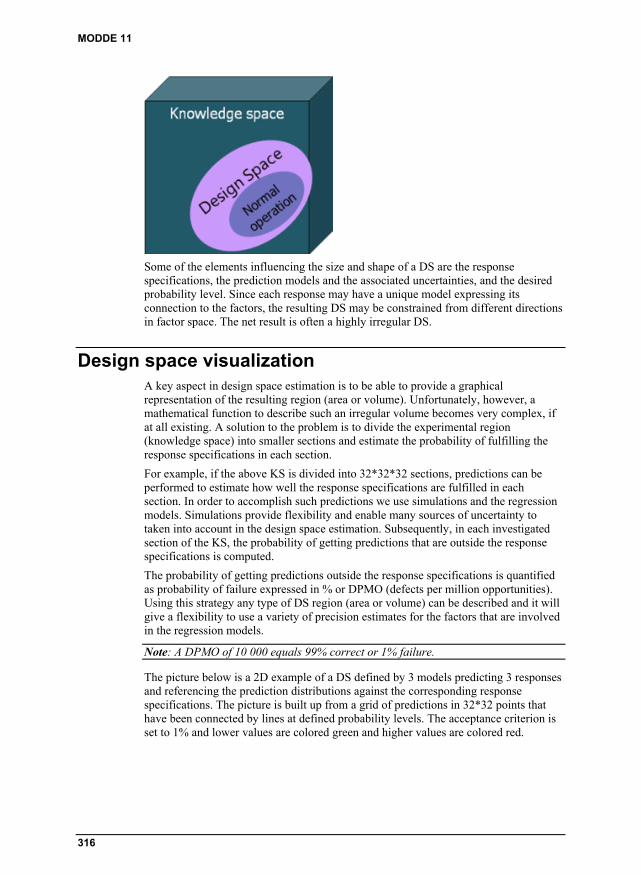
MODDE 11

316

Some of the elements influencing the size and shape of a DS are the response specifications, the prediction models and the associated uncertainties, and the desired probability level. Since each response may have a unique model expressing its connection to the factors, the resulting DS may be constrained from different directions in factor space. The net result is often a highly irregular DS.

Design space visualization A key aspect in design space estimation is to be able to provide a graphical representation of the resulting region (area or volume). Unfortunately, however, a mathematical function to describe such an irregular volume becomes very complex, if at all existing. A solution to the problem is to divide the experimental region (knowledge space) into smaller sections and estimate the probability of fulfilling the response specifications in each section.

For example, if the above KS is divided into 32*32*32 sections, predictions can be performed to estimate how well the response specifications are fulfilled in each section. In order to accomplish such predictions we use simulations and the regression models. Simulations provide flexibility and enable many sources of uncertainty to taken into account in the design space estimation. Subsequently, in each investigated section of the KS, the probability of getting predictions that are outside the response specifications is computed.

The probability of getting predictions outside the response specifications is quantified as probability of failure expressed in % or DPMO (defects per million opportunities). Using this strategy any type of DS region (area or volume) can be described and it will give a flexibility to use a variety of precision estimates for the factors that are involved in the regression models.

Note: A DPMO of 10 000 equals 99% correct or 1% failure.

The picture below is a 2D example of a DS defined by 3 models predicting 3 responses and referencing the prediction distributions against the corresponding response specifications. The picture is built up from a grid of predictions in 32*32 points that have been connected by lines at defined probability levels. The acceptance criterion is set to 1% and lower values are colored green and higher values are colored red.

Design space appendix

317

As mentioned in the Statistical appendix, MODDE supports three interval estimates. The default setting in this context is the Prediction interval. The selected interval type will strongly influence the size of the resulting DS region (area or volume).

Furthermore, the size of the resulting DS region will also be critically influenced by which type of disturbance is applied to the factor settings. The DS estimate rendered in the above plot assumes that the factors can be set exactly numerically, and that the only disturbance applied to the factors in the simulations is in line with the size of the model error [y = f(x) + e].

Alternatively, if it is assumed that the factors cannot be set exactly numerically, it is possible to invoke an additional source of uncertainty in the simulations, i.e., according to what is termed Precision in factor setting in the Factor Definition dialog box. For instance if Air can be set with a precision of +/- 8 kg/h and EGR% with +/- 0.4 % the DS region will shrink somewhat (see plot below).

Elaboration with various types of factor precision can be done in the Setpoint analysis tool. In the Setpoint analysis changing the precision is done by altering the Std. dev. or Low/High values. If the DS is created from another entrance than Setpoint analysis on the Optimizer contextual tab, the factor precision used is the one originally specified in the Factor definition dialog box used for the design specification. Adjustment of this precision can be done in the Factor definition dialog box or in the Setpoint analysis.

MODDE 11

318

In-depth assessment of Design Space The Design Space (DS) graphs presented in the previous paragraph are simplistic in the sense that they are only two-dimensional representations of a complicated reality. An in-depth and more realistic assessment of a DS can be done by using the Design Space Explorer tool available after running the Optimizer. When first launching this tool a Settings page is opened, where it is possible to modify default settings for a number of options that have a profound impact on the course of the design space estimation.

As seen, the simulations by default take model error into account but not the factor precision. Resolution is the number of sections that each factor range will be divided into. Iterations is the number of simulations in each section for each response. DPMO limit is the criterion for specifying the DS region.

If more than 5 factors are available the default selection will be the 5 with the highest factor contribution. The factor contribution is calculated as the prediction variation over all responses and is presented in the optimizer Setpoint tab.

The number of calculations will increase exponentially with the number of factors and the selected resolution. A recommendation is to start with resolution 16 and 50 000 simulations but for a final documentation the recommendation is to use 32 as resolution and leave the computer for an overnight calculation if necessary.

MODDE can address a maximum of 644 data points, but may take many hours before completion.

Factors/Resolution Res 8 Res 16 Res 32 Res 64

3 factors Possible Possible Possible Possible

4 factors Possible Possible Possible Possible

5 factors Possible Possible Not possible Not possible

6 factors Possible Possible Not possible Not possible

7 factors Possible Not possible Not possible Not possible

Design space appendix

319

When clicking OK in the Design Space Explorer dialog box, simulations commence and finally results are presented in terms of a Design Space Explorer window. This window consists of three parts.

The main part is a 2D plot showing the size and shape of the DS as viewed in the subspace defined by the two factors chosen for the X- and Y-axes.

The second part is the Properties pane in which axis factors and constant factors can be selected. For each factor fixed at a constant value a slider is available to facilitate a step-less browsing from one setting to another.

The third part is a Design space hypercube overview functionality, which is useful when trying to comprehend the size and shape of the investigated DS in the dimensions beyond the 2D representation of the corresponding plot.

Apart from a visualization of the design space in two dimensions, the design space explorer provides two additional graphical tools, i.e.,

a cross-hair symbol that indicates the position of the robust setpoint and

a dotted frame that shows the placement of the so called design space hypercube.

The design space hypercube corresponds to the volume in which all factor combinations can be used without compromising the response specifications. Its extension in the 2D plot is given by the dotted frame, and its elongation across all dimensions is shown by the green color in the Design space hypercube overview. Note that the hypercube range can be changed interactively by clicking and dragging the low or high end for the range of a particular factor.

So, in summary, the green color in the Hypercube range field designates the mutual ranges within which all factors can be changed at the same time and without further restrictions. Slightly wider individual ranges are patterned by the black T-lines, which represent the allowable range of a process factor, while keeping all other factors constant at their setpoint value.

MODDE 11

320

For more comprehensive evaluation and documentation, the design space estimation results can be exported to a text file by Creating a list (Tools | List or right-click and click Create list). The output is an N-dimensional DS description.

Proven acceptable ranges A closely related idea to the design space concept is the notion of proven acceptable ranges (PAR) for the factors. ICH Q8 defines a PAR as "a characterized range of a process parameter for which operation within this range, while keeping other parameters constant, will result in producing a material meeting relevant quality criteria". In fact, the PAR notion fits well into the capabilities of MODDE. There are three modes in which to state PAR in MODDE:

1 – Based on the robust setpoint The hypercube range of the design space explorer is used. The black T-lines extending out from the robust setpoint coordinate indicate the individual ranges for the factors, i.e., the largest allowable range of a process parameter, while keeping all other parameters constant at their setpoint value. A full numerical documentation is available using Create list with the Optimizer window active (Tools tab or right-click).

2 – Based on the dotted hypercube frame

The dotted frame in the Design Space Explorer plot designates the largest possible regular hypercube that can be inserted into the irregular design space volume. How this regular hypercube extends into many dimensions is given by the green bars seen in the Hypercube range part in the picture above. The green bars mark the mutual ranges within which all factors can be changed at the same time and without further restrictions.

Design space appendix

321

3 – Based on setpoint analysis 3 is reminiscent of 1, but is based on a distribution around a setpoint. Such distributions are attained using the Setpoint analysis functionality in MODDE. The details of the Setpoint analysis tool are given in the next paragraph. Briefly, Setpoint analysis is available after running the optimizer. It outputs the estimated acceptable range for the factors at every given setpoint.

Setpoint analysis Setpoint analysis is available after running the optimizer. This tool can estimate the tolerance available for the factors at every given setpoint. It is an excellent platform for analysis of any given setting and also for imposing practical adjustments to the allowable factor ranges and evaluating the consequences of such changes.

In the presentation below the robust setpoint is the start, and from that co-ordinate the factor ranges are expanded until the DPMO limitation criterion is reached.

Factor variations possible to use are presented as Estimated acceptable ranges. Various types of distributions and interval estimates can be used in the estimation; the default is a normal distribution and a prediction interval.

In this example, the responses that limit the widening of the factor ranges are Fuel and Soot as these responses first reach the DPMO limit of 10 000 DPMO. All estimations are based on the regression models and with the prediction interval.

Properties - Setpoint analysis In the property page settings can be adjusted. The most important one is the Interval type used for the predictions and the acceptance criterion (DPMO). Because the predictions are based on simulations the stability in the results is dependent on the number of simulations. The default settings aim to give a reasonable estimate within a quite short time. The result can thus vary between simulations. To get a more stable result for documentation we recommend increasing the Acceptable range simulations and Response profile simulations.

MODDE 11

322

Monte Carlo simulations The Monte Carlo simulations are:

random factor settings according to the selected distribution,

around their optimum value but within the Low and High limits,

followed by predictions of the responses. In this case 50 000 predictions are performed. The distribution as well as the number of simulations and the range can be changed by the user.

The resulting distributions can be presented as a histogram, one for each response.

Evaluate the results and make necessary adjustments If the result in some way is not satisfactory, one option can be to change the starting point for the DS search (selected setpoint). Another option is to lock some factor ranges where setting tighter specifications won’t be a problem. For more, see the Setpoint validation for robustness testing subsection later in this chapter.

For alternative start points it can be preferable to step back to the optimizer and select another start point based on Log(D), DPMO and Design Space evaluation. The modeling results, e.g. Coefficient Plot, can also be an information source to finding alternatives. All settings can be changed in the Setpoint analysis window for a user controlled search in order to find the most appropriate solution.

The setpoint shown below is a movement of the factor setting Needlelift to a higher setpoint.

The alternative factor settings give results within specifications but with narrower estimated acceptable ranges than for the previously proposed starting point. The alternative factor settings might be preferred for practical reasons.

Design space appendix

323

How to find the best Design Space 1. Develop the best model for each response.

2. Check the residual distribution for outliers or unresolved structures.

3. Find the optimal settings for the factors that comply with the response criteria (optimizer).

4. Check if the proposed optimal factor settings are critical (close to a limit) or in a safe region.

5. Perform a Robust Setpoint analysis.

6. Decide on the interval type and the acceptance level; default settings are Prediction interval and 10 000 DPMO.

7. Make an evaluation of the complete Design Space with Design Space Explorer.

8. Decide on how to express the PAR, from a setpoint or as a selected hypercube inserted into the Design Space.

9. Evaluate the results and make necessary adjustments using DS analysis and Setpoint analysis.

10. Set your preferred factor specifications with any necessary practical adjustments.

11. Document the final results.

Setpoint validation for robustness testing According to the FDA: "VALIDATION OF ANALYTICAL PROCEDURES: Definition and terminology. The robustness of an analytical procedure is a measure of its capacity to remain unaffected by small, but deliberate variations in method parameters and provides an indication of its reliability during normal usage."

Setpoint validation is a way to test if the system investigated is robust against disturbances in the investigated region. Setpoint validation can be found on the Predict tab.

The aim of robustness testing is to evaluate if a process, or a system, performs satisfactory even when some influential factors are allowed to vary. In other words, we want to investigate the system’s sensitivity (or preferably lack of sensitivity) to changes in certain critical factors. The advantages with having a robust process or system include simpler process control, a known range of applicability and an ensured quality of the product or process.

A robustness test is usually carried out before the release of an almost finished product, or analytical system, as a test to ensure quality. MKS Umetrics recommends the use of DOE for robustness testing and such a design is usually centered on the factor combination, which is currently used for running the analytical system, or the process. We call this the setpoint. The setpoint may have been found through a screening design, an optimization design, or some other identification principle, such as written quality documentation. The aim of robustness testing is, therefore, to explore robustness close to the chosen setpoint.

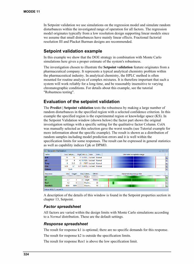
MODDE 11

324

In Setpoint validation we use simulations on the regression model and simulate random disturbances within the investigated range of operation for all factors. The regression model originates typically from a low resolution design supporting linear models since we assume that small disturbances have mainly linear effects. Fractional factorial resolution III and Placket Burman designs are recommended.

Setpoint validation example In this example we show that the DOE strategy in combination with Monte Carlo simulations here gives a proper estimate of the system's robustness.

The investigation chosen to illustrate the Setpoint validation feature originates from a pharmaceutical company. It represents a typical analytical chemistry problem within the pharmaceutical industry. In analytical chemistry, the HPLC method is often mounted for routine analysis of complex mixtures. It is therefore important that such a system will work reliably for a long time, and be reasonably insensitive to varying chromatographic conditions. For details about this example, see the tutorial "Robustness testing".

Evaluation of the setpoint validation The Predict | Setpoint validation tests the robustness by making a large number of random disturbances in the specified region with a selected confidence criterion. In this example the specified region is the experimental region or knowledge space (KS). In the Setpoint Validation window (shown below) the factor part shows the original investigation settings with a specific setting for the qualitative factor Column. ColA was manually selected as this selection gave the worst results (see Tutorial example for more information about the specific example). The result is shown as a distribution of random samples including model prediction errors and it is well within the specification limits for some responses. The result can be expressed in general statistics as well as capability indices Cpk or DPMO.

A description of the details of this window is found in the Setpoint properties section in chapter 13, Setpoint.

Factor spreadsheet

All factors are varied within the design limits with Monte Carlo simulations according to a Normal distribution. These are the default settings.

Response spreadsheet

The result for response k1 is optional; there are no specific demands for this response.

The result for response k2 is outside the specification limits.

The result for response Res1 is above the low specification limit.

Design space appendix

325

The result for response PlateN(2) is above the low specification limit

From the above we conclude that this system is robust against disturbances in the factors for Res1 and PlateN(2). k2 is not robust against disturbances in the factors.

Final adjustments Setpoint validation can be used to estimate the maximum accepted variability in factors that still predict all results within the specifications.

The problem in the described example is response k2. The requirement for k2 is that less than 1%, corresponding to DPMO = 10 000, of the predictions may be outside the specification limits.

There are constraints when handling this type of situation;

Which factors affect the result?

How can we adjust the factor limits without causing too much problems in the normal use of the procedure?

First we have to check the model to understand which factors are the most influential. The model has to be significant for an adjustment in factor ranges to have an effect on the result distribution.

In this example the model for k2 is very significant and the most important factor is Acetonitrile (ACN).

Assuming that the factor Temperature is easy to control with a narrower range we start with this factor by adjusting temperature to +/- 0.5 °C. At the same time we can open the Role for ACN to Free. This instruction together with the specification limit for k2 (DPMO = 10 000) will give an estimate of a range for ACN where we can predict that the system is robust according to the specifications. The picture next here displays the result of the change in settings.

MODDE 11

326

The proposed settings for ACN are now 25.45 to 26.55 and the estimated distribution for k2 is 9 680 hits outside the specification limits.

A final step might be to make an adjustment of the factor settings to some practical new specification within the range for ACN, for instance 25.5 to 26.5. The result shown below implies that the critical response k2 will have 0.58% of future predictions outside the specifications.

Result statistics for k2

To open the response histogram, click the histogram symbol to the far right in the Setpoint validation window.

In the Select responses box, select which responses to display.

Design space appendix

327

To view statistics, create a list from the Setpoint validation window (Tools tab, or right-click).

A more detailed description of this example is found in the tutorial named "Robustness Testing".

329

Stability design appendix

Introduction A pharmaceutical product in storage may change its quality characteristics with time. Hence, it is important to know how well a product retains its quality characteristics over the life span of the product. A product is considered stable as long as its quality characteristics remain within specifications. The shelf life of a product corresponds to the number of days it remains stable at the recommended storage conditions. The process of collecting experimental data for estimating and verifying a product's shelf life is called stability testing.

As outlined by the ICH guidelines (1, 2), design of experiments (DOE) is a cornerstone technology in stability testing. This because DOE enables to spread out informative experiments in the critical factors across the time span that is encompassed by the stability test. The normal duration of a stability test is 36 months, with testing time points occurring at 0, 3, 6, 9, 12, 18, 24 and 36 months.

In addition to the obvious Time factor, stability testing often involves between 2-5 additional factors, for instance strength, container size and/or fill. These factors can be quantitative or qualitative in nature and be studied at two or more levels. As with regular DOE protocols, the number of factor combinations grows rapidly with increasing number of levels of the factors. A full study stability test is one in which all factor combinations are tested for every time point. It is easily realized that this may not be a suitable design approach especially when the number of factor combinations is large. Instead reduced designs can be used, in which only a subset of the factor combinations is tested at a given time point.

The prevailing approach to stability testing implies that full testing of all factor combinations is done at 0 and 36 months, and that reduced testing is carried out at all other time points (3, 6, 9, 12, 18 & 24 months). Reduced testing means that only subsets of the factor combinations are tested. Various reductions can be used and common reductions are the one-half reduction and the one-third reduction. This approach is known as matrixing.

Ideally, the various reductions tested at 3, 6, 9, 12, 18 & 24 months should be complementary, so that all factor combinations indeed are investigated at least once in each type of reduction. Furthermore, it is advantageous if all levels of any qualitative factor are exploited the same number of times in each reduction. This last point is often referred to as balancing. Balancing subsets of factor combinations so that they are perfectly complementary inside each type of reduction is the real challenge in stability testing, and although balancing is worth striving for it is not always straightforward to accomplish.

MODDE 11

330

With the release of MODDE 11, MKS Umetrics introduces a new class of reduced combinatorial designs that are perfectly complementary when superimposed on top of one another. This new design family is described in the Reduced combinatorial designs subsection in the Design appendix. In this appendix we shall describe how the so called complementary combinatorial designs are especially suited to the needs of stability testing, and how they bring a vast array of stability testing scenarios into one common framework. The data set used is illustrative of the main principles for data analysis.

Setting up a stability test In order to launch a stability testing design, on the File tab, click New, and under Specific application design, click Stability design.

This will open up the Design Wizard, with one factor (Time) pre-defined. As shown below, the default settings for Time are 0, 3, 6, 9, 12, 18, 24 and 36 months. The settings of the Time factor can be changed manually and up to 24 settings (time points) can be entered.

In the design wizard all factors to be investigated are defined. Besides Time our example deals with the three factors Strength of API (quantitative, two levels), Batch of API (qualitative, three batches) and Primary packaging of tablet (qualitative, four packaging variants). A full factorial design in Strength, Batch and Primary packaging corresponds to 24 (=2*3*4) factor combinations.

Stability design appendix

331

The next step in the design wizard deals with response definition. For each response it is possible to enter specifications in terms of Min, Target and Max values. Only one response is used in our example, the amount of impurities, which has a Max specification of 2%. This Max setting refers to the desired situation at the last studied time point.

Define stability design setup time point designs When factors and responses have been defined, the next step corresponds to setting up the stability testing design. This is done using the Define stability design setup page. The basis for this page is a timeline running from left to right where all time points previously set for the Time factor are listed as separate columns.

In our example, full testing of all factor combinations (24 runs) is proposed for 0, 12 and 36 months, whereas reduced testing is proposed at all other time points. We can see that two reductions are suggested. Two half-reductions of 12 runs – denoted design sets B:1 and B:2 -- are scheduled for 18 and 24 months, and three one-third reductions of 8 runs -- denoted design sets C:1, C:2 and C:3 -- are scheduled for 3, 6 and 9 months.

You can interactively change which reduction to use at a given time point. Replicates and center points can also be changed at this stage. Moreover, it is also possible to generate new reductions and distribute them across time as deemed appropriate. A fourth reduction may be added by clicking Add reduction (not illustrated here). Up to 9 reductions are supported.

MODDE 11

332

Define stability design setup, Design sets The lower part of the stability design setup page shows which reductions are eligible and how many runs they contain. By clicking Expand all (the plus sign) more details are provided.

For each design set, the augmented list of details informs about whether the design set in question is balanced or not, its condition number and the number of runs it contains.

Stability design appendix

333

Stability design worksheet By clicking Finish on the stability design setup page, the worksheet of the stability design is created. In our example, the worksheet comprises 120 runs. An excerpt is shown below. Compared with the worksheet of a conventional DOE protocol there are some minor differences. First of all, there is a new column, the second from left, denoted Combination ID. There will be as many Combination IDs as there are factor combinations (excluding the Time factor), i.e. 24 in our example; 25 if there are center points. Secondly, the column denoted Exp Name has a modified naming structure for each experimental run, a modified structure which indicates which factor combination and time point applies for each row in the worksheet. Finally, there are two list boxes which enable subset selections of the experiments. Subset selections can be accomplished based on the factor combinations and time points.

MODDE 11

334

Early stage data analysis – trajectory trending The default data analytical method is MLR, which is a sound choice provided that there are no major disturbances to the geometry of the stability design. Data analysis of measured data can be done at any stage of the duration of the stability test. In the early stages, say after 6 or 9 months, the focus lies on trending, i.e., understanding what will likely be the development trajectory of the response with time. This kind of assessment is done with a simple regression model, usually involving only Time as the single model term.

Subset selection of experiments representing different time spans is easily accomplished by using the Included time points and Included combination boxes of the worksheet. With all experiments included, the calculations automatically include the experiments that have response values and ignores those without.

Below, we illustrate how main trend analysis of the Impurities trajectory can be done incrementally after 3, 6, 9 and 12 months. The Factor Effect Plot, available on the Predict tab, is an indispensable tool in this respect. Gradually, as more and more data points become available, we can see that the precision – in terms of a narrowing interval estimate1 – in the predicted level of Impurities is improved.

However, judging from this early stage trend analysis, we are at risk of violating the 36 months Max setting of the response. The question is whether any of the other factors display a significant influence on the response? This is addressed in the next section.

1 By default, the interval estimate presented in the Factor Effect plot is the Confidence interval (aka average) with the setting 95%. This interval estimates where 95% of the future average predictions will be found. The confidence interval is common practice in mainstream regression analysis. In stability testing, however, the use of another type of interval estimate, the so called prediction interval (aka individual), is more prevalent. The prediction interval suggests where we can expect a future individual sample to be predicted. Also a third variant is available in MODDE; it is a tolerance interval and reflects the estimation of future populations of predictions. More information about the various interval estimates is found in the Interval estimates subsection in the Statistical appendix. In order to swap between the three alternative intervals estimates, right click the plot, click Properties and use the Interval estimation tab. The type of interval estimate used is listed in the footer of the graph.

Stability design appendix

335

MODDE 11

336

Early stage data analysis – assessment of factor effects

The main conclusion from the previous trend analysis was a worrying increase in the predicted level of Impurities towards the end of the stability test. Because of this undesired future trajectory it is of relevance to investigate the impact of the other three factors on the response variable. In order to accomplish this assessment, the regression model must be modified so that it includes all possible main and interaction effects; on the Home tab, click Edit model.

Stability design appendix

337

The regression model, based on all 0-12 months measurements, was updated using the full set of main and interaction effects. A substantial increase in R2 was the result, from 0.506 (Time factor only) to 0.768 (all main and interaction terms). This increase in the explained variance points to the fact that one or a few of the additional model terms exhibit a significant impact on the response variable. This can be further assessed using the regression coefficient plot.

The regression coefficient plot shows a few noteworthy facts. It is evident that Time is the strongest factor. It has a positive coefficient meaning that the numerical value of the response variable increases with Time. However, there is also a statistically significant influence of the Batch factor; in particular, the third batch exhibits a strong positive influence on Impurities. Moreover, the coefficient plot reveals a strong interaction effect between Time and Batch 3. The other two factors, Package and Strength, do not influence the response variable.

MODDE 11

338

The Interaction Plot is a useful tool to get a graphical appraisal of an interaction. Based on the plot below there is no doubt that Batch 3 has a detrimental impact on Impurities compared with the other two batches.

The main conclusion after analyzing the 0-12 months segment of data is that Batch 3 is associated with a rapid and unacceptable increase in the level of Impurities. As a consequence this batch should be excluded from further consideration in the stability test. It will not comply with the final 36 months acceptance criterion.

Late stage data analysis The early stage data analysis revealed that Batch 3 would not comply with the final acceptance criterion. Hence, all existing samples (0-12 months) and all future samples (18-36 months) including this factor setting need to be excluded from the data analysis. The easiest way to accomplish this is to sort the MODDE worksheet according to the Batch factor. Mark the Batch column, right click and click Sort descending. This will give you a worksheet where all runs involving Batch 3 are listed first. Then simply mark all rows containing Batch 3 and in the Incl/Excl column select Excl.

Stability design appendix

339

Before fitting the model on a larger time span (0-24 months) the model was again edited by reverting to using the Time as the single factor. The resulting Factor Effect plot for Time is seen here. The conclusion is that the 36 months acceptance criterion most likely will be met.

Summary and discussion The new design family for stability testing is based on reduced combinatorial design sets that are perfectly complementary when superimposed on top of one another. The complementarity principle is illustrated by the three design cubes shown here. The design cubes represent a three-factor problem where one factor has two levels, one three levels and one four levels. The full factorial design in these three factors comprises 2*3*4 = 24 runs. Each design cube represents a one-third fraction in 8 runs. Mathematically, the three one-third fractions are equivalent and when superimposed on top of one another they perfectly pattern the corresponding full factorial design. This is the gist of the new approach to stability testing in MODDE, i.e., the ability to fraction any stability design problem into reductions of various degree (design sets of one-half, one-third, one-fourth, … reductions) that are balanced and perfectly complementary.

MODDE 11

340

It should be emphasized that what is written and discussed in this appendix relates to the context of work performed in early development. Usually, in early development it is of relevance to explore many factors at many levels, and as early as possible to discover factors and factor settings that clearly encode unfavorable instability in the tested product. One of the interesting aspects of using the novel stability designs in MODDE is that all levels of all factors are tested at an early stage even though reduced design sets are employed. And this gives the beneficial asset of allowing the user to detect and remove elements in the experimental scheme that cause instability. Such early removal of uninteresting elements and zooming-in on critical features in the stability testing facilitate optimal use of the available testing resources.

References

1. Anonymous, Bracketing and matrixing designs for stability testing of new drug substances and products, ICH Guideline Q1D.

2. Anonymous, Evaluations for stability data, ICH Guideline Q1E.

341

References

1. R.A. Fisher, “Statistical methods, experimental design, and scientific inference”, A re-issue (J. H. Bennett, Ed.), Oxford University Press, Oxford, England, (1990).

2. G.E.P. Box, W. G. Hunter, and J. S. Hunter, “Statistics for experimenters”, Wiley, New York, (1978).

3. G.E.P. Box, The collected works, Vol 1. (G.C. Tiao, Ed.), Wadsworth Advanced Books and Software, Belmont, CA, 1985.

4. Morgan, Chemometrics: Experimental Design, ACOL, London, and Wiley, New York, (1991).

5. Wold, “Soft modeling, The basic design and some extensions”, In Vol. II of K-G. Jöreskog and H. Wold, Ed.s. Systems under indirect observation, Vol.s I and II, North-Holland, Amsterdam, (1982).

6. Wold, A. Ruhe, H. Wold and W. J. Dunn III, “The Collinearity Problem in Linear Regression. The Partial Least Squares Approach to Generalized Inverses”, SIAM J. Sci. Stat. Comput. 5, 735-743, (1984).

7. Höskuldsson, “PLS Regression Methods”, J.Chemometrics, 2, 211-228, (1988).

8. Wold. “Cross validatory estimation of the number of components in factor and principal components models”, Technometrics 20, 397, (1978).

9. Draper and Smith, “Applied Regression Analysis”, Second Edition, Wiley, New York.

10. Cornell, “Experiments with Mixtures”, New York: Wiley, (1990).

11. Cox, “A Note on Polynomial Response Functions for Mixtures”, Biometrica, 58, 155-159, (1971).

12. Crosier, “Mixture Experiments: geometry and Pseudo components”, Technometrics, 26, 209-216, (1984).

13. Kettaneh-Wold, “Analysis of mixture data with partial least squares”, Chemometrics and Intelligent laboratory Systems, 14, 57-69, (1992).

14. Rechtschaffner R.L., Saturated fractions of 2n and 3n factorial designs, Technometrics, 1967, Vol.9, N°4, 569-575.

15. Ing-Marie Olsson, Erik Johansson, Martin Berntsson, Lennart Eriksson, Johan Gottfries, and Svante Wold, “Rational DOE-protocols for 96 well plates”, Chemometrics and Intelligent Laboratory Systems, 2006.

16. Doehlert, D.H., “Uniform shell designs”, Journal of the Royal Statistical Society, 1970, Serie C, N°19, 231-239.

17. Snee, “Test Statistics for Mixture Models”, Technometrics, Nov. 1974.

MODDE 11

342

18. Cohen, Jacob (1988). Statistical power analysis for the behavioral sciences. Hillsdale, New-Jersey, 2nd edition.

19. Hoenig, J. M. and Heisey, D. M. (2001). The abuse of power: The pervasive fallacy of power calculations for data analysis. The American Statistician, 55, 19-24.

20. Liu , Xiaofeng Steven (2014). Statistical Power Analysis for the Social and Behavioral Sciences: Basic and Advanced Techniques. Taylor & Francis, 1st edition.

21. O’Keefe, Daniel J. (2007). Post Hoc Power, Observed Power, A Priori Power, Retrospective Power, Prospective Power, Achieved Power: Sorting Out Appropriate Uses of Statistical Power Analyses. Communication Methods and Measures, 1(4), 291-299.

22. Zumbo, Bruno D. and Hubley, Anita M. (1998). A note on the misconceptions concerning prospective and retrospective power. The Statistician, 47, 385-388.

23. Cederkvist, H.R., Aastveit, A.H., and Naes, T., The importance of functional marginality in model building – A case study, Chemometrics and Intelligent Laboratory Systems, 87, 98-106, 2007.

24. Draper, Norman and Smith, Harry, Applied Regression Analysis, Second Edition, Wiley, New York, 1981.

25. Golub, Gene H. and Van Loan, Charles F, Matrix Computations, The Johns Hopkins University Press, Baltimore, 1983.

26. Rao, C. R. (1947), Factorial Experiments Derivable from Combinatorial Arrangements of Arrays, Journal of the Royal Statistical Society, Supplement,9, 128–139.

27. Wang, J. C., and Wu, C. F. J. (1992), Nearly Orthogonal Arrays With Mixed Levels and Small Runs, Technometrics, 34, 409–422.

28. Hongquan Xu (2002), An Algorithm for Constructing Orthogonal and Nearly-Orthogonal Arrays With Mixed Levels and Small Runs, Technometrics, 44, 356–368.

29. Anonymous, Bracketing and matrixing designs for stability testing of new drug substances and products, ICH Guideline Q1D.

30. Anonymous, Evaluations for stability data, ICH Guideline Q1E.

343

Index

344

2 2D

Contour ........................................... 175 Design space ................... 102, 184, 223 Sweet spot ............................... 180, 221

3 3D

Onion plots ...................................... 124 Response surface ............................. 177 Rotate .............................................. 198 Scatter ..................................... 130, 170 Sweet spot ....................................... 180 Zoom and rotate .............................. 198

4 4D

Contour ................................... 101, 176 Design space ................... 102, 184, 223 Sweet spot ............................... 180, 221

A Abbreviation

Factor definition ................................ 22 Investigation options ......................... 70 Response definition ........................... 30

About MODDE ....................................... 5

Absolute limits ............................ 216, 217

Accelerators ....................................... 7, 79

Activate MODDE .................................... 5

Add Component ........................................ 96 Experiment ...................................... 128 Factor .......................................... 22, 56 Inclusions ........................................ 112 Plot element .................................... 195 Response ........................................... 30 Terms .................................... 56, 59, 94 To favorites ..................................... 206 To report ......................................... 206

Add plot element ................................. 195

Add to favorites ................................... 206

Add to report ....................................... 206

Alternative setpoints ............................ 215

Analysis advisor .................................. 189

Analysis phase ................................... 2, 16

Analysis wizard Coefficients ....................................... 89 Histogram ......................................... 86 Interaction test .......................... 91, 257 Observed vs. predicted ...................... 93 Replicates .......................................... 85 Residuals normal probability ............ 92 Square test ................................. 90, 257 Summary of fit .................................. 88 Tests statistical appendix ................ 257 Toolbar.............................................. 84 What is? ............................................ 84

Analyze tab .......................................... 141

ANOVA .............................. 146, 147, 252

Arrange windows ................................ 193

Arrow .................................................. 197

Audit trail ................................ 70, 73, 190

Augmenting designs .............................. 56

Automatic Auto update predictions .................. 170 Cross-validation significance rules . 248 Fit ...................................................... 96 Update of plots and lists .................. 206 Update predictions .......................... 170

Autoscale modifier ................................ 31

Axial designs ....................................... 293

Axis ............................................. 200, 201

B Background ......................................... 202

Balanced .............................. 285, 288, 303

Block Blocks ............................................... 40 BlockV ............................................ 128 D-Optimal ....................................... 279 Fixed ............................................... 279 Interaction ......................................... 40 Mark ............................................... 197 Option ............................................... 70 Orthogonal ...................................... 276 Random ........................................... 279 RSM ................................................ 278 Screening ........................................ 277

Block interaction ............................. 40, 41

Blocks.............................................. 40, 41

Box-Behnken ....................................... 289

Box-Cox ...................................... 149, 263

Index

345

C Candidate set

Constrained ..................................... 111 Create new ........................................ 43 Edit .................................................... 43 Imported ...................................... 43, 61 Layer runs ......................................... 45 Max size ............................................ 68 New design ....................................... 61 Onion .............................................. 302 Open ................................................ 123 Regular ............................................ 296 Size ................................................... 43

Case sensitivity ...................................... 17

CCC ..................................................... 288 Blocking .......................................... 278 Constraints ...................................... 213 Design ............................................. 288 Star distance ...................................... 40

CCC constraints ................................... 213

CCF ..................................................... 288

CCO..................................................... 288

Center points ......................................... 39

Central Composite Circumscribed ....... 288

Central Composite Face ...................... 288

Central Composite Orthogonal ............ 288

Classical mixture designs .................... 293

Close ...................................................... 68

Coding qualitative factors .................... 258

Coefficients Compact format ........................ 74, 256 Confidence intervals ................. 74, 256 Extended format ........................ 74, 256 Interaction test ........................... 91, 257 Normalized................................ 74, 256 Plot .................................................. 155 PLS orthogonal ......................... 74, 256 Scaled and centered ................... 74, 256 Square test ................... 74, 90, 256, 257 Statistical appendix ................... 74, 256 Unscaled ................................... 74, 256

Color ANOVA table ................................. 146 Axes ................................................ 200 by variable ...................................... 130 Contour ........................................... 204 Correlation matrix ........................... 133

Format plot ..................................... 199 List .................................................... 78 Mini toolbar ........................................ 8 Onion by layer ................................ 124 Scatter ............................................. 130 Setpoint properties .......................... 230 Sweet spot ....................................... 180 Worksheet ....................................... 128

Column formatting .............................. 205

Combinatorial designs ......................... 286

Compact coefficients ............. 74, 256, 257

Compatibility ....................................... 301

Complement design Doehlert ............................................ 58 D-Optimal ......................................... 59 Estimate squares terms ...................... 57 Fold over ........................................... 57 Inclusions vs. complement .............. 111 New ................................................... 56 New complement design ................... 56 PBSS to PB ....................................... 56 Rechtschaffner .................................. 56 What is? ............................................ 56 With inclusions ............................... 112

Condition number ................ 134, 136, 259

Confidence Interval for coefficients ..... 74, 256, 257 Interval for predictions .................... 261 Interval type and probability levels ... 75 Level ................................................. 70

Confoundings ...................................... 122 by variable ...................................... 130

Constraints Candidate set ................................... 111 Define ............................................. 109 Define graphically........................... 110 Define in spreadsheet ........................ 28 Mixture constraint ........................... 292 Modify graphically ......................... 110 Page .................................................. 28 Qualitative or multilevel ................... 29 Supported .......................................... 29 Types of .................................... 29, 109 Why ................................................ 109

Context menu ...................................... 206

Contextual tab ......................................... 6

Contour Customize ............................... 178, 204 Format plot ..................................... 204

MODDE 11

346

From optimizer ............................... 220 Labels .............................................. 178 Open ................................................ 175 Options .................................... 178, 180 Resolution ....................................... 178 Response surface ............................. 177 Scale equally ................................... 178 Wizard ............................................. 178

Controlled .............................................. 25

Convention ............................................ 17

Coordinate reader ................................ 199

Copy ...................................................... 65

Correlation Matrix ............................................. 133 Plot .................................................. 133

Cpk ...................................................... 281

Cross-validation rules .......................... 248

Cube plot ............................................. 115

Cubic terms ......................................... 249

Curvature diagnostics plot ................... 131

Customize plot Axes ................................................ 200 Axis and title font............................ 201 Axis X and Y .................................. 201 Background ..................................... 202 Column ........................................... 205 Contour ........................................... 204 Error bars ........................................ 205 Gridlines ......................................... 202 Labels .............................................. 204 Legend ............................................ 203 Limits and regions ........................... 203 Mini toolbar .................................... 199 Open ................................................ 199 Restore ............................................ 196 Save ................................................ 196 Styles .............................................. 205 Templates ........................................ 196 Tick Marks ...................................... 201 Titles ............................................... 203

Customize ribbon .................................. 10

D Default options ...................................... 70

Default plot formatting ........................ 196

Defects Per Million Opportunities ....... 281

Degrees of freedom ..................... 249, 253

Deleted studentized residuals ........ 76, 258

Derived responses Define ............................................... 32 Operators and functions .................... 34 Qualitative factors ............................. 35 Sets of variables ................................ 33 Syntax ............................................... 33

Description button ................................. 37

Descriptive statistics .................... 134, 136

Design Box-Behnken .................................. 289 CCC ................................................ 288 CCF ................................................. 288 CCO ................................................ 288 Classical mixture designs ................ 293 Doehlert .......................................... 290 Evaluation ....................................... 298 Fractional factorial .......................... 285 Fractional factorial at three levels ... 286 From candidate set ............................ 61 From scores ....................................... 62 Full factorial............................ 285, 303 Full factorial at three levels ............. 288 Mixture ........................................... 291 Onion .............................. 287, 289, 301 Plackett Burman .............................. 286 Plackett Burman Super-Saturated ... 286 Rechtschaffner ........................ 287, 289 RED-MUP .............................. 287, 289

Design matrix .............................. 116, 117

Design phase ........................................... 2

Design region ...................................... 115

Design runs............................................ 39

Design space Appendix ........................................ 315 Documentation ........................ 318, 320 Explorer .................................. 227, 318 From Home tab ............................... 102 From Optimizer tab ......................... 223 From Setpoint analysis .................... 236 How to find the best ........................ 323 Monte Carlo simulations ................. 322 Options............................................ 185 Predict tab ....................................... 184 What is? .................................. 315, 316

Design summary .......................... 119, 121

Design tab ........................................... 105

Design wizard .................................. 21, 84

Index

347

Desirability .................................. 308, 310

Desirability settings ............................. 308

Determinant ................................. 295, 298

DF ................................................ 249, 253

DF residual .................. 134, 136, 249, 253

Distance to model ................................ 165

Distance to target ................................. 273

Distribution Factor .............................................. 234 Histogram ....................................... 137 Response ......................................... 235 Setpoint analysis ............................. 280 Setpoint Factor spreadsheet............. 232

DModY ............................................... 165

Dockable windows .............................. 189

Doehlert designs .................................. 290

D-Optimal Algorithm ........................................ 297 Balanced ........................................... 42 Blocking .......................................... 279 Candidate set ................................... 302 Complement ...................................... 59 Criteria ........................................ 44, 48 Design evaluation ............................ 298 Design runs span ............................... 42 Design summary ..................... 119, 121 Design wizard page ........................... 41 Implementation ............................... 297 Onion candidate set ........................... 47 Onion designs ................................. 301 Regenerate design ........................... 124 Repetitions ........................................ 42 What is? .......................................... 295 When? ............................................. 296

D-Optimal onion Candidate set ............................. 47, 302 Designs ................................... 287, 289 From candidate set ............................ 61 From scores ....................................... 62 Layers max ........................................ 68 Layers page ....................................... 45 Plots ................................................ 124

DPMO ................................. 274, 275, 281

DPMO default limit ............................... 77

DS Appendix ......................................... 315 Documentation ........................ 318, 320 Explorer .......................................... 227

From Home tab ............................... 102 From Optimizer tab ......................... 223 From Setpoint analysis .................... 236 How to find the best ........................ 323 Monte Carlo simulations ................. 322 Options............................................ 185 Predict tab ....................................... 184 What is? .................................. 315, 316

Dynamic profile................................... 220

E Edit menu ................................................ 9

Edit model ............................................. 94

Effects List .................................................. 162 Main effect ...................................... 161 Normal probability .......................... 160 Open ............................................... 159 Plot .................................................. 159

Eigenvalue ........................................... 259

Email mip .............................................. 67

Encrypt .................................................. 52

Error bars ............................................. 205

Estimate squares terms .......................... 57

Evaluate ....................................... 134, 136

Evaluation plot .................................... 208

Exclude ........................................ 103, 199

Execute folder ..................................... 192

Experiment name ................................. 128

Experiment number ............................. 128

Experimental cycle .............................. 2, 4

Experimental design Create ................................................ 55 Objective ........................................... 13 What is? ............................................ 13

Experimental region ............................ 115

Experiments ......................................... 128

Export favorites configuration ............. 192

Extended Axial ............................................... 293 Design matrix .......................... 116, 117 List presentation .................. 70, 73, 190 Model list .......................................... 94

External variability ...................... 131, 276

Extreme vertices .......................... 119, 121

MODDE 11

348

F Factor

Add ................................................... 21 Advanced .......................................... 26 Contribution .................................... 275 Definition .............................. 22, 23, 26 Delete ................................................ 21 Distribution ..................................... 234 Edit .................................................... 21 Effects ..................................... 173, 174 Formulation ..................................... 291 Max number ...................................... 23 Mixture and process ........................ 291 Mixture definition ........................... 291 Modify ...................................... 21, 106 Name ................................................. 17 Precision ........................................... 25 Qualitative ................................. 35, 258 Scaling ............................................ 249 Setting ............................................... 23 Spreadsheet ............................. 213, 232 Transformation .................................. 26 Type .................................................. 23 Use for factor .................................... 25 What is? .......................................... 106

Factor distribution ............................... 234

Factorial designs .......... 285, 286, 288, 303

Favorites Add to favorites .............................. 206 Create folder ................................... 192 Delete .............................................. 192 Export ............................................. 192 Import ............................................. 192 Open and tile ................................... 192 Rename ........................................... 192 Restore ...................................... 81, 193 Treat folder as item ......................... 192 Window ........................................... 192

F-distribution ............................... 147, 148

File tab ................................................... 51

Filler ................................................ 23, 25

Fit Goodness of fit ........................ 249, 253 Lack of fit ....................................... 148 Methods ................................ 15, 96, 97 Mixture ............................................. 97 MLR ................................................ 245 Model .......................................... 17, 96 Plots .................................................. 97 PLS ................................................. 246

Summary list ................................... 145 Summary plot .................................. 143

Fixed block factor ................................ 279

Fold over ............................................... 56

Foldover ................................................ 56

Footer .................................................. 203

Format plot Axes ................................................ 200 Axis and title font ........................... 201 Axis X and Y .................................. 201 Background ..................................... 202 Column ........................................... 205 Contour ........................................... 204 Error bars ........................................ 205 Footer .............................................. 203 Gridlines ......................................... 202 Header ............................................. 203 Labels ............................................. 204 Legend ............................................ 203 Limits and regions .......................... 203 Mini toolbar .................................... 199 Open ............................................... 199 Restore ............................................ 196 Save ................................................ 196 Styles .............................................. 205 Tick Marks ...................................... 201 Titles ............................................... 203

Formulation ......................................... 291

Fractional factorial Complement ...................................... 56 Designs ........................................... 285

Free-form selection ............................. 197

Full factorial Design ..................................... 285, 303 Three levels ..................................... 288

Full screen ........................................... 193

G Gallery ..................................................... 6

G-efficiency ......................... 119, 121, 298

General options General tab ........................................ 68 List options ....................................... 78 Restore .............................................. 81

General page Factor definition ................................ 23 MODDE options ............................... 68

Index

349

Generate report Add to report ................................... 206 Report ............................................... 54

Generators ........................................... 114

Goodness of fit ............................ 249, 253

Graeco-Latin square ............................ 286

Gridlines .............................................. 202

H Hat matrix .................................... 249, 253

Header ................................................. 203

Help About MKS Umetrics ....................... 82 Help .......................................... 4, 5, 81 Interactive help ................................... 4 MKS Umetrics on the Web ................. 5

Hierarchy ............................................. 249

High limit ...................................... 30, 213

Histogram ...................................... 86, 137

Home tab ............................................... 83

Hypercube ........................................... 227

Hyperlink ............................................. 242

Hyper-triangles .................................... 290

I Image ................................................... 240

Import Candidate set ............................. 61, 302 Design from file ................................ 55 Favorites configuration ................... 192 Inclusions to worksheet ................... 112 Scores ................................................ 62 Worksheet to inclusions .................. 113

Inclusions And design augmentation ................ 299 As part of design ............................. 112 Edit .................................................. 113 Open ................................................ 111 vs. complement design .................... 111

Individual response analysis ................ 235

Insert in report Add to report ................................... 206 Hyperlink ........................................ 240 Picture ............................................. 240 Template ......................................... 240

Insert rows ........................................... 128

Installation ............................................... 1

Interaction plot .................................... 163

Interaction test ............................... 91, 257

Interactive exclude tool ............... 103, 199

Interval estimates ................................... 75

Interval type and probability levels ....... 75

Investigation Change options ................................. 70 Compatibility .............................. 10, 62 Managing .......................................... 10 Mip ................................................... 10 What is? ............................................ 10

Irregular region .................................... 299

K Keyboard ............................................... 10

Keyboard shortcuts ...................... 7, 78, 79

KeyTips ............................................. 7, 79

L Labels .................................................. 204

Lack of fit ............................................ 148

Latent structures .................................. 246

Layers overlap ....................................... 45

L-designs ............................................. 286

Legend ................................................. 203

Licenses ................................................... 5

Limit optimization ............................... 309

Limits .................................................. 203

Line style ......................................... 8, 205

Linked responses ................................... 35

List Create .............................................. 206 Presentation....................................... 70

Loading plots ............................... 163, 164

Lock Contour levels ................................. 178 Investigation ..................................... 52

LOF ..................................................... 148

Log Determinant .................................... 298 In audit trail............................... 73, 190

LogDet ................................................ 298

MODDE 11

350

LogDetNorm ....................................... 298

Low limit ....................................... 30, 213

M Main effect plot ................................... 161

Manage licenses ...................................... 5

Mark .................................................... 197

Maximum runs ............................ 119, 121

Mid-range .............................................. 26

Mini toolbar ............................................. 8

Mip-file ................................................. 10

Missing data ........................................ 250

Mixture And process factors ......................... 291 Constraint ........................................ 292 Contour ........................................... 175 Cox .......................................... 264, 265 Data in MODDE ............................. 264 Design space ................................... 184 Designs ........................................... 291 Experimental region ........................ 292 Factor definition .............................. 291 Factors statistical appendix ..... 264, 265 Fit ...................................................... 97 Irregular region ............................... 299 Models .................................... 264, 265 Prediction plots ............................... 171 Slack variable model ............... 264, 265 Sweet spot ....................................... 180

MLR Fit methods ....................................... 15 Formula ........................................... 245

MLR scaling Mid-range ......................................... 26 Ortogonal .......................................... 26 Responses ......................................... 31 Statistical appendix ......................... 249 Unit variance ..................................... 26

MODDE About .................................................. 5 Starting ................................................ 2

MODDE options General tab ........................................ 68 List options ....................................... 78 Restore .............................................. 81

Model Distance to ...................................... 165 Edit .................................................... 94

Error ................................................ 283 Fit ...................................................... 96 Hierarchy ........................................ 249 Individual .......................................... 96 List .................................................... 94 Q2 ................................................... 251 R2 ................................................... 251 Reproducibility ............................... 252 Saturated ................................. 249, 253 Select .......................................... 37, 40 Singular ........................................... 249 Validity ........................................... 252 What is? ............................................ 13

Monte Carlo ........................................ 280

Multilevel factor .................................... 23

Multiple Linear Regression ........... 15, 245

Multiplot Overview plot ................................... 99 Select responses .............................. 206

Multivariate ........................................... 62

N Near orthogonal array .......................... 303

Network installation ................................ 5

New Application designs ........................... 60 Complement design .......................... 56 Design from candidate set ................. 61 Design from scores ........................... 62 D-Optimal ....................................... 124 Experimental design ......................... 55 External design ................................. 55 Investigation ..................................... 10 RED-MUP .................................. 60, 62 Report ............................................... 54 Worksheet from file .......................... 55

Next component .................................... 96

NOA .................................................... 303

Normal probability Effects ............................................. 160 Residuals ......................................... 151

Normalized Coefficients ....................... 74, 256, 257 LogDetNorm ................................... 298

Notes ................................................... 189

N-plot Effects ............................................. 160 Residuals ......................................... 151

Index

351

Number format ...................................... 70

Number of decimals .............................. 27

N-value ................................................ 251

O OA ....................................................... 303

Objective Select................................................. 35 Settings ............................................. 40 What is? .......................................... 115

Observed vs. predicted .......... 93, 100, 154

Onion Candidate set ................................... 302 Designs ................................... 287, 289 Generate ...................................... 61, 62 Layers max ........................................ 68 Plots ................................................ 124 Screening ........................................ 301

Open all items ...................................... 192

Open investigation ................................. 63

Operators - derived responses ................ 34

Optimization Blocking .......................................... 278 Design ............................................... 14 Focus ....................................... 273, 311 Limit ....................................... 270, 309 Objective ........................................... 35 Robust ............................................. 225 Target ...................................... 272, 310

Optimizer Alternative setpoints ....................... 215 Conditional tab ................................ 219 Contour ........................................... 220 Copy to predictions ......................... 208 Definition ........................................ 269 Design space ................................... 223 Desirability.............. 211, 270, 272, 273 f(ds) ................................................. 308 Factor spreadsheet ........................... 213 Introduction ..................... 207, 269, 307 List .................................................. 218 Objective tab ................................... 210 Objectives ............................... 208, 308 Overall distance to target ................ 273 Properties ................................ 216, 217 Response spreadsheet ...................... 210 Search function ............................... 312 Specifications .................................. 311 Summary ......................................... 218

Sweet spot ....................................... 221 Tab .................................................. 219 Weight ............................................ 308 Window .......................................... 208

Options Customize ................................... 78, 79 Investigation Options ........................ 70 List options ....................................... 78 MLR scaling ..................................... 26 MODDE options ............................... 68 Restore .............................................. 81 Types ................................................ 68

Organization ............................................ 6

Orthogonal Array ............................................... 303 Blocking .......................................... 276 Correlation ...................................... 133 Scaling .............................................. 26

Orthogonal array ................................. 303

Outliers Distance to model ........................... 165 Residuals normal probability plot ... 151 Score plots ...................................... 164

Output window Open automatically ........................... 68 Show or hide ................................... 189 What is? .......................................... 189

Overall distance to target ..................... 273

Overlay prediction ............................... 171

Overview plot ........................................ 99

P Partial Least Squares ............. 15, 245, 246

Password protect ................................... 52

Paste design ........................................... 35

Paste unformatted in report ................. 240

PBSS ................................................... 286

Picture ................................................. 240

Placeholders View ............................................... 242 Window .......................................... 243

Plackett Burman Blocking .......................................... 277 Designs ........................................... 286 PBSS designs .................................. 286

Plackett Burman Super-Saturated ........ 286

MODDE 11

352

Plate-Size ......................................... 60, 62

Plot Copy .................................................. 65 Preview ............................................. 65 Quality .............................................. 65 Save .................................................. 65 Size ................................................... 65

Plot formatting Axes ................................................ 200 Axis and title font............................ 201 Axis X and Y .................................. 201 Background ..................................... 202 Column ........................................... 205 Contour ........................................... 204 Error bars ........................................ 205 Footer .............................................. 203 Gridlines ......................................... 202 Header ............................................. 203 Labels .............................................. 204 Legend ............................................ 203 Limits and regions ........................... 203 Mini toolbar .................................... 199 Open ................................................ 199 Restore ...................................... 81, 196 Save ................................................ 196 Styles .............................................. 205 Templates ........................................ 196 Tick Marks ...................................... 201 Titles ............................................... 203

Plots Box-Cox .......................................... 149 Coefficients ..................................... 155 Contour ........................................... 101 Design space ................................... 102 DModY ........................................... 165 Effect............................................... 159 Histogram ....................................... 137 Interaction ....................................... 163 Main effect ...................................... 161 Observed vs. predicted .................... 100 Overview ........................................... 99 PLS ................................................. 163 Replicates ........................................ 138 Residuals normal probability .......... 151 Scatter ............................................. 130 Summary of fit ................................ 143 Sweet spot ....................................... 180 VIP .................................................. 166

PLS Fitting with PLS ........................ 15, 246 Orthogonal coefficients ..... 74, 256, 257 PLS coefficients .............................. 263

PLS summary list ............................ 145 Scaling .............................................. 27 Scheffé .............................................. 96 Scores and loadings ................ 163, 262 Summary plots ........................ 143, 144

Potential terms ..................................... 297

Power estimation ........................... 41, 303

Predict Contour ........................................... 175 Design space ................................... 184 Factor effects .......................... 173, 174 List .................................................. 170 Optimizer ........................................ 208 Prediction plots ............................... 171 Residuals vs. predicted.................... 152 Scatter plot ...................................... 170 Setpoint validation .......................... 187 Spreadsheet ..................................... 170 Sweet spot ....................................... 180 Tab .................................................. 169

Prediction Copy from optimizer ....................... 208 Formula ........................................... 261 Phase ................................................... 4 Plots ................................................ 171 Spreadsheet ..................................... 170 Using the model ................................ 17 With model error ............................. 283

Predictive factor distribution ............... 234

PRESS ................................. 248, 249, 253

PRESS/SSY........................................... 15

Preview .................................................. 65

Print Format ............................................... 67 Quality .............................................. 65

Probability contour plot ............... 184, 315

Process and mixture factors ................. 291

Process Capability Index ..................... 281

Process factors ..................................... 269

Product ID ............................................... 5

Program limits ....................................... 68

Properties Contour ........................................... 178 Dialog ............................................. 206 Optimizer ................................ 216, 217 Page ................................................ 206 Report generator ............................. 244

Index

353

Setpoint ........................................... 230

Protect investigation .............................. 52

Q Q2 ........................................................ 251

Qualitative factors Coding at > 2 levels ........................ 258 Definition .......................................... 23 In derived response ................... 35, 258

Quantitative ........................................... 23

Quantitative multilevel .......................... 23

Quick Access Toolbar 9, 10, 63, 64, 65, 67

Quick start Analysis wizard ................................. 84 Design wizard ................................... 84

R R2 ........................................................ 251

Random factor ..................................... 279

Raw residuals ................................ 76, 258

Recalculate scale ................................. 200

Recent Folders .............................................. 63 Investigations .................................... 63

Rechtschaffner designs ................ 287, 289

Recommended designs .......................... 37

RED-MUP ............................... 60, 62, 287

Reduced Axial ............................................... 293 CCC ................................................ 288 CCF ................................................. 288

Reduced combinatorial designs ........... 286

Reference mixture ............................... 113

References ..................................... 19, 341

Regions ................................................ 203

Register ................................................... 5

Regular responses .................................. 31

Remove Encryption ......................................... 52 Footer .............................................. 203 Header ............................................. 203 Model term ...................................... 199 Placeholder...................................... 242 Timestamp ...................................... 203

Replicate ANOVA .......................................... 146 Design ............................................... 39 Plot ............................................ 85, 138 Tolerance .......................................... 68

Report Add to report ................................... 244 Create ................................ 54, 237, 238 File .................................................. 239 Formatting ...................................... 242 Home .............................................. 240 Open ................................. 54, 237, 238 Picture ............................................. 240 Placeholders window ...................... 243 Properties window .......................... 244 Start ................................... 54, 237, 238 Template ......................................... 239 View ............................................... 242 What is? .......................................... 237 Window .......................................... 239

Report generator ............ 54, 237, 238, 239

Report writer ................. 54, 237, 238, 239

Reproducibility .................................... 252

Reset Factor precision ................................ 25 Factors columns .............................. 106 Favorites ........................................... 81 Interface customization ..................... 10 Messages ........................................... 81 Model ................................................ 94 Optimizer factor settings ................. 208 Optimizer response settings ............ 208 Plot formatting .......................... 81, 196 Report template ....................... 239, 240 Rotation .......................................... 198

Residual standard deviation ................. 252

Residuals Default ............................................ 150 Gallery ............................................ 100 List .................................................. 154 Normal probability .................... 92, 151 Type definition .......................... 76, 258 Types .............................................. 150 vs. predicted response ..................... 152 vs. run order .................................... 153 vs. variable plot ............................... 153

Response Add ................................................... 30 Box ................................................. 206 Definition .......................................... 30

MODDE 11

354

Derived ............................................. 32 Distribution setpoint ........................ 235 Exclude using modifier ..................... 31 Linked ............................................... 35 Name ................................................. 17 Profile ............................................. 220 Regular ...................................... 31, 108 Response box .................................. 206 Select............................................... 206 Setpoint spreadsheet ........................ 233 Spreadsheet ..................................... 108 Surface ............................................ 177 Surface modeling .............................. 14 Transform ......................................... 31

Restore Favorites ................................... 81, 196 Interface customization ..................... 10 Plot formatting .......................... 81, 196 Report template ....................... 239, 240

Ribbon Customization ................................... 10 Description .......................................... 6

Robust optimization Design space explorer ..................... 227 Find ................................................. 225 Results..................................... 226, 227

Robust setpoint Design space explorer ..................... 227 Find ................................................. 225 Results..................................... 226, 227

Robustness ........................................... 323

Rotate .................................................. 198

RSD ..................................................... 252

RSM Blocking .......................................... 278 Design ............................................... 14 Objective ........................................... 35

Run list ................................................ 215

Run order ............................................. 131

S Safe region ........................................... 313

Saturated models ......................... 249, 253

Save Audit trail ............................ 70, 73, 190 Inclusions ........................................ 112 Investigation ................................ 64, 65 Plot formatting ................................ 196 Plot or list .................................... 64, 65

Templates ........................................ 196

Scaling Coefficients ....................... 74, 256, 257 Formula ........................................... 249 MLR ................................................. 26 PLS ................................................... 27

Scatter Loading ........................................... 164 Model data ...................................... 130 Prediction ........................................ 170 Score ............................................... 164

Scheffé .................................................. 97

Score plots ........................................... 164

Screen reader ....................................... 199

Screening Designs ........................................... 285 Number factors ................................. 13

ScreenTips ............................................... 6

Search function .................................... 307

Select All ................................................. 7, 79 Default factor .................................... 70 Fit method ......................................... 96 In plot .............................................. 197 Objective ........................................... 35 Responses ....................................... 206

Selected setpoint .................................. 214

Send as attachment ................................ 67

Send by email ........................................ 67

Sensitivity analysis ...................... 274, 275

Set Run order ....................................... 131

Setpoint Alternative setpoints ....................... 215 Design space ................................... 236 Factor ...................................... 232, 234 Introduction............................. 229, 230 Properties ........................................ 230 Response ................................. 233, 235 Robust ............................. 225, 226, 227 Selected ........................................... 214 Setpoint analysis ............................. 228 Setpoint validation .......................... 187 Summary ......................................... 235

Settings CCC .................................................. 37 Factor ................................................ 23 Optimizer ........................................ 208

Index

355

Plot .................................................. 199 Restore .............................................. 81 Save ................................................ 196 Split objective ................................... 40

Shortcut menu ..................................... 206

Show Contour levels ................................. 185 Expanded RED-MUP ........................ 68 Placeholders .................................... 242 ScreenTips ........................................ 10 Units .................................................. 68

Significant term ..................................... 89

SIMCA .................................................. 62

Simplex Mixture ........................................... 292 Optimizer search function ............... 274

Size preview .......................................... 65

Slack variable .............................. 264, 265

Sort ...................................................... 129

Specific application designs .................. 60

Specification .......................................... 93

Split button .............................................. 6

Split objective ........................................ 35

Spreadsheet .......................... 170, 213, 232

Square test ..................................... 90, 257

Stability design ............................ 302, 333

Stability testing .................................... 329

Standard error ...................................... 261

Standard fit ............................................ 96

Standardized residuals ................... 76, 258

Star distance .......................................... 40

Starting MODDE ..................................... 2

Starting simplexes ............................... 274

Statistical appendix .............................. 245

Status bar ............................................. 189

Styles ................................................... 205

Summary of fit Analysis wizard ................................. 88 List .................................................. 145 Plots .................................. 97, 141, 143 PLS ................................. 143, 144, 145

Surface Onion plots ...................................... 124

Response surface ............................ 177 Rotate .............................................. 198 Sweet spot ....................................... 180 Zoom and rotate .............................. 198

Sweet spot ........................... 102, 180, 221

Symbol style .................................... 8, 205

Syntax derived response ........................ 34

T Tagushi .................................................. 13

Target In optimizer ..................................... 210 Optimization ................................... 310 Response definition ........................... 30

Templates Plot .................................................. 196 Report ..................................... 239, 240

Theme .............................................. 78, 79

Threshold ............................................ 133

Tick marks ........................................... 201

Timestamp ........................................... 203

Titles ................................................... 203

Toolbar .................................................. 84

Tools tab .............................................. 195

Tooltip ..................................................... 6

Total runs .............................................. 39

Traditional designs ................................ 55

Transform ........................................ 26, 31

Treat folder as item ............................. 192

U Uncentered coefficients ................. 74, 256

Unconfound ........................................... 40

Uncontrolled .......................................... 25

Undo .................................................... 103

Unit variance ................................... 26, 27

Units ...................................................... 68

Update Constraint graphically ..................... 110 Placeholder ..................................... 242 Plots and lists .................................. 206 Prediction spreadsheet .................... 170 Report ............................................. 240

Update of plots and lists ...................... 206

MODDE 11

356

User interface ........................................ 10

Usp-file .................................................. 62

V Validity ................................................ 252

Variable importance ............................ 166

Variable plot ........................................ 153

View tab .............................................. 189

View windows ..................................... 189

VIP ...................................................... 166

W WC plots .............................................. 262

Web ......................................................... 5

Weight in optimizer ..................... 216, 217

Windows Analysis advisor .............................. 189 Arrange ........................................... 193 Audit trail .................................. 73, 190 Favorites ......................................... 191

Notes ............................................... 189 Output ............................................. 189

Wizard Analysis wizard ................................ 84 Contour plot wizard ........................ 178 Design space wizard ....................... 185 Design wizard ................................... 84 Sweet spot wizard ........................... 180

Worksheet Add experiments ............................. 128 Adding inclusions ........................... 112 Colors ............................................. 128 Derived responses ............................. 32 Design matrix .......................... 116, 117 Missing values ................................ 128 Open ............................................... 128 Run Order ....................................... 131 Sort ................................................. 128 Tab .................................................. 127

Write report ................... 54, 237, 238, 239

Z Zoom ............................................... 8, 198