modal logics of ordered trees - uva · modal logics of ordered trees ulrich endriss 2003 ......
TRANSCRIPT

Modal Logics of Ordered Trees
Ulrich Endriss


Modal Logics of Ordered Trees
Ulrich Endriss
2003
A thesis submitted to the University of Londonfor the degree of Doctor of Philosophy
King’s College LondonDepartment of Computer Science

Revised Edition (March 2003)

Abstract
This thesis makes a contribution to the area of modal and temporal logics, an impor-tant family of non-classical logics that have found numerous applications in computerscience and several other disciplines. Temporal logics, in particular, have been appliedvery successfully in the area of systems specification and verification. However, theselogics often do not support the notion of refinement in a natural manner. There is nosimple way to extend a given system specification, expressed in a standard temporal logicsuch as, for instance, propositional linear temporal logic, by the specification of a newsubsystem. It is therefore important to extend available formalisms in ways that allowfor the representation of complex systems evolving over time in a modular fashion.
To this end, we propose to equip propositional linear temporal logics with a ‘zoomfeature’ in the following manner. If we extend the class of modal frames of this logic byadding a vertical accessibility relation to connect every time point with a new time line,we obtain a tree-like structure where the children of each node form a linear order. Moreprecisely, we obtain a modal logic with frames that are ordered trees. The horizontalaccessibility relation is still given a temporal interpretation, while the vertical allowsus to move between different levels of abstraction, that is, between a system and itssubsystems. Our logic provides modal operators working both along the branches of atree and along the order declared over the children of a node.
The body of this work is devoted to the theoretical study of this modal logic ofordered trees. In particular, we are concerned with an axiomatic characterisation of ourlogic complementing its semantics-driven definition and with proving its decidability.


Acknowledgements
Many people have, in one way or another, played their part in the genesis of this thesis.Individual contributions range from very concrete support with my scientific endeavoursto just being nice and making my years as a PhD student a very enjoyable time. In whatfollows, I shall mostly concentrate on the former type of contribution, but hope everyoneelse will get the message as well.
First and foremost, I should like to thank Dov Gabbay, my thesis supervisor, forhis encouragement and support throughout my studies, for being a great inspirationfrom Day One, for letting me do things my way, and for always sharing his insightson logic and people. The Group of Logic and Computation at King’s College (nowthe Group of Logic, Language and Computation) has provided the perfect environmentfor my studies. Everyone in the group, our numerous visitors, and many others in theDepartment of Computer Science have contributed to a very pleasant and stimulatingworking atmosphere. This includes, in particular, my first generation of office mates in542: Stefan Schlobach, Odinaldo Rodrigues, and Wilfried Meyer-Viol. I’m also indebtedto Hans Jurgen Ohlbach for his help and support whilst being my second thesis supervisorat the beginning of my PhD studies, before he moved on to Munich.
Stefan Schlobach, Wilfried Meyer-Viol, and Raquel Fernandez have read large partsof various earlier incarnations of this thesis and their feedback has substantially im-proved the final product. Thanks are also due to Misha Zakharyaschev, Agi Kurucz,and Valentin Shehtman for answering a plethora of questions on modal logic; and to theregulars at our logic reading group: David Gabelaia, Roman Kontchakov, Corinna Elsen-broich, and George Metcalfe. I have also greatly benefited from discussing my work withthe many people I met along the way, in particular Martina Kullmann, Carsten Lutz,Enrico Franconi, Alessandro Artale, Anuj Dawar, and Ian Hodkinson. Naza Aguirredeserves a special mention for showing me that the software engineering people still needa lot more temporal logic. Finally, I would like to thank Howard Barringer and RobinHirsch for having agreed to examine this work.
On a more personal note, this seems like a good place to acknowledge the part myparents, Micha and Moni Endriß, have had in all of this.
London, January 2003 U.E.

The research reported here has been generously funded by the UK Engineering and Phys-ical Sciences Research Council (EPSRC) through a number of projects: GR/L91818/01(grant holders: D. Gabbay and H. J. Ohlbach), GR/R45369/01 (M. Zakharyaschev,D. Gabbay, and I. Hodkinson), and GR/N23028/01 (D. Gabbay), all at King’s CollegeLondon. The writing-up of the thesis was completed while the author was employedat Imperial College London on a research project funded by the European Union undergrant reference number IST-2001-32530 (grant holders at Imperial: F. Toni and F. Sadri).
Contents
1 Zooming in 11.1 Adding a Zoom to Linear Temporal Logic . . . . . . . . . . . . . . . . . . 11.2 Thesis Overview . . . . . . . . . . . . . . . . . . . . . . . . . . . . . . . . 10
2 Modal and Temporal Logics 132.1 Introducing Modalities . . . . . . . . . . . . . . . . . . . . . . . . . . . . . 132.2 Possible World Semantics . . . . . . . . . . . . . . . . . . . . . . . . . . . 182.3 Axioms and Correspondences . . . . . . . . . . . . . . . . . . . . . . . . . 242.4 Temporal Logic . . . . . . . . . . . . . . . . . . . . . . . . . . . . . . . . . 312.5 Bibliographic Notes . . . . . . . . . . . . . . . . . . . . . . . . . . . . . . . 37
3 Semantic Characterisation 393.1 Syntax and Semantics . . . . . . . . . . . . . . . . . . . . . . . . . . . . . 393.2 Some Defined Operators . . . . . . . . . . . . . . . . . . . . . . . . . . . . 483.3 Correspondences . . . . . . . . . . . . . . . . . . . . . . . . . . . . . . . . 503.4 Ontological Considerations . . . . . . . . . . . . . . . . . . . . . . . . . . 553.5 General Models and P-morphisms . . . . . . . . . . . . . . . . . . . . . . 603.6 Loosely Ordered Trees . . . . . . . . . . . . . . . . . . . . . . . . . . . . . 673.7 Summary . . . . . . . . . . . . . . . . . . . . . . . . . . . . . . . . . . . . 94
4 Axiomatic Characterisation 974.1 Axioms and Rules . . . . . . . . . . . . . . . . . . . . . . . . . . . . . . . 974.2 Some Derived Theorems . . . . . . . . . . . . . . . . . . . . . . . . . . . . 1084.3 Completeness without Descendant Modalities . . . . . . . . . . . . . . . . 1134.4 Alternatives . . . . . . . . . . . . . . . . . . . . . . . . . . . . . . . . . . . 1414.5 Summary . . . . . . . . . . . . . . . . . . . . . . . . . . . . . . . . . . . . 145
5 Decidability 1475.1 Monadic Second-order Logic . . . . . . . . . . . . . . . . . . . . . . . . . . 1475.2 Finite Binary Trees . . . . . . . . . . . . . . . . . . . . . . . . . . . . . . . 1595.3 Discretely Ordered Trees . . . . . . . . . . . . . . . . . . . . . . . . . . . . 1635.4 General Ordered Trees . . . . . . . . . . . . . . . . . . . . . . . . . . . . . 1695.5 Summary . . . . . . . . . . . . . . . . . . . . . . . . . . . . . . . . . . . . 182
vii

viii Contents
6 Zooming out 1856.1 Extensions . . . . . . . . . . . . . . . . . . . . . . . . . . . . . . . . . . . . 1856.2 Summary of Main Results . . . . . . . . . . . . . . . . . . . . . . . . . . . 1926.3 Open Problems . . . . . . . . . . . . . . . . . . . . . . . . . . . . . . . . . 193
Appendices 197
A Relations and Orders 199A.1 Relations . . . . . . . . . . . . . . . . . . . . . . . . . . . . . . . . . . . . 199A.2 Linear Orders . . . . . . . . . . . . . . . . . . . . . . . . . . . . . . . . . . 200
B Derivations 203B.1 Proof of Lemma 4.8 . . . . . . . . . . . . . . . . . . . . . . . . . . . . . . 203
Bibliography 205
List of Figures 211
List of Tables 213
Index 215
Chapter 1
Zooming in
In this thesis we develop a new modal logic to represent complex systems evolving overtime in a modular fashion. As will be explained in this chapter, this new logic maybe regarded as the result of extending well-known linear temporal logic by a seconddimension that allows us to zoom into states and thereby model events associated withthem in more detail. In this sense, our logic may be described as an extended temporallogic. From a more abstract point of view, our logic is best characterised as a modal logicof ordered trees.
In this first chapter we motivate the enterprise of developing such a logic in the firstplace and give an informal outline of some of the main results reported in the sequel.The final section also provides a compact overview of the thesis as a whole, organised bychapters.
1.1 Adding a Zoom to Linear Temporal Logic
Why? What do we mean by adding a zoom to temporal logic and why would anyonewant to do something like this? We begin our explanation with a story, the story of Mary.Mary was an aspiring young software engineer who was working for an up-and-cominginformation technology company offering state-of-the-art software solutions to its clientsand profitable revenue to its shareholders. One day, not that long ago, the company’syoung and dynamic marketing department managed to secure a major contract with anew heavy-weight client. It was their biggest software development contract yet and alot (if not everything) depended on its successful completion. Mary was appointed ChiefEngineer on the project.
Most people would have been intimidated by that much responsibility. Not Marythough. She was not only a true professional, but had also benefited from an excellenteducational system which had provided her with a very respectable academic background.Mary had completed a degree in Computer Science at one of the country’s finest univer-sities. She was fluent in all the major programming languages, knew her computer insideout, and commanded an intimate knowledge of all phases of the software development
1

2 Chapter 1. Zooming in
process, be it design, implementation, or evaluation of the final product. She was evengood at maths. But was all of this going to be enough for this new and highly criticalproject? The central question seemed to be: How do you make sure the system willreally do what it is supposed to?
Mary was lucky. In her final year at university, besides all the programming lan-guages, software engineering, databases, and computer architecture, she had also at-tended a class on non-classical logics, which was at the time taught by a very famouslogic professor. In fact, she probably did not even realise just how lucky she had been,because most of the time the famous professor was tied up in research, which regularlyinvolved writing books, proving ground-breaking new results, and even developing wholenew schools of thought. But this particular year he did teach and Mary enjoyed thecourse very much. One of the subjects that made a lasting impression on her was thefield of temporal logics. She could remember it very well. Temporal logics were aston-ishingly simple, yet extremely powerful; full of mathematical depth and beauty, but also— as she had realised by now — of immediate industrial relevance. Several of the bigcompanies leading the market were already using this exciting new technology to helpthem develop provably correct software systems. Mary knew she had to find out moreabout temporal logic, and she had to do so quickly. This she owed to her company’sshareholders.
Temporal logic. So what is temporal logic? In short, a temporal logic is a formalsystem to reason about propositions that change their truth value over time. In thecontext of designing reliable software artefacts, examples for propositions would be sen-tences such as ‘the variable x currently has value 542’ or ‘the file critical.xml is currentlybeing written on by process 4711’. A proposition may be either true or false at any givenpoint in time.
Naturally, the notion of time itself will be central to our understanding of temporallogics. A simple yet useful model of time would be the following:
t0
•t1
•t2
•t3
•t4
•t5
// // // // //
That is, we can think of time as a sequence of time points or states. The first one, t0,denotes the beginning of time and after that we have one state for each and every naturalnumber. Of course, this is a very simplified if not artificial model of time. It does, forinstance, not take into account special relativity theory or the latest findings in quantumphysics. But for the basis of a logic intended to describe a sequence of events, such asthose taking place while a complex software system is being executed, this seems quiteappropriate.1
1We are painting a somewhat simplified picture of the field of temporal logics here. The particular
logic we are in the process of describing is known as propositional linear temporal logic. In fact, at this
point we restrict our attention to the future-fragment of propositional linear temporal logic over discrete
flows of time and we shall not consider the so-called until -operator either. A fuller account of the area
of (modal and) temporal logics is given in Chapter 2.
1.1 Adding a Zoom to Linear Temporal Logic 3
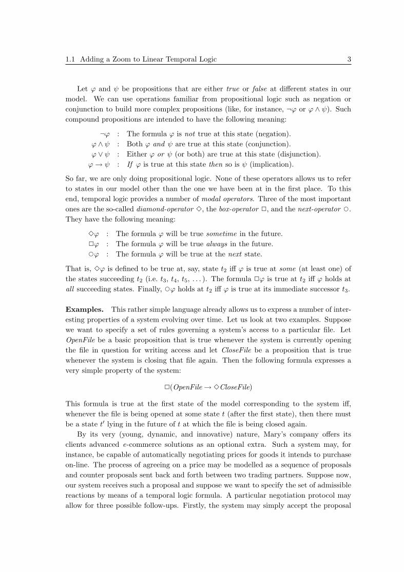
Let ϕ and ψ be propositions that are either true or false at different states in ourmodel. We can use operations familiar from propositional logic such as negation orconjunction to build more complex propositions (like, for instance, ¬ϕ or ϕ ∧ ψ). Suchcompound propositions are intended to have the following meaning:
¬ϕ : The formula ϕ is not true at this state (negation).ϕ ∧ ψ : Both ϕ and ψ are true at this state (conjunction).ϕ ∨ ψ : Either ϕ or ψ (or both) are true at this state (disjunction).ϕ→ ψ : If ϕ is true at this state then so is ψ (implication).
So far, we are only doing propositional logic. None of these operators allows us to referto states in our model other than the one we have been at in the first place. To thisend, temporal logic provides a number of modal operators. Three of the most importantones are the so-called diamond-operator 3, the box-operator 2, and the next-operator e.They have the following meaning:
3ϕ : The formula ϕ will be true sometime in the future.2ϕ : The formula ϕ will be true always in the future.eϕ : The formula ϕ will be true at the next state.
That is, 3ϕ is defined to be true at, say, state t2 iff ϕ is true at some (at least one) ofthe states succeeding t2 (i.e. t3, t4, t5, . . . ). The formula 2ϕ is true at t2 iff ϕ holds atall succeeding states. Finally, eϕ holds at t2 iff ϕ is true at its immediate successor t3.
Examples. This rather simple language already allows us to express a number of inter-esting properties of a system evolving over time. Let us look at two examples. Supposewe want to specify a set of rules governing a system’s access to a particular file. LetOpenFile be a basic proposition that is true whenever the system is currently openingthe file in question for writing access and let CloseFile be a proposition that is truewhenever the system is closing that file again. Then the following formula expresses avery simple property of the system:
2(OpenFile → 3CloseFile)
This formula is true at the first state of the model corresponding to the system iff,whenever the file is being opened at some state t (after the first state), then there mustbe a state t′ lying in the future of t at which the file is being closed again.
By its very (young, dynamic, and innovative) nature, Mary’s company offers itsclients advanced e-commerce solutions as an optional extra. Such a system may, forinstance, be capable of automatically negotiating prices for goods it intends to purchaseon-line. The process of agreeing on a price may be modelled as a sequence of proposalsand counter proposals sent back and forth between two trading partners. Suppose now,our system receives such a proposal and suppose we want to specify the set of admissiblereactions by means of a temporal logic formula. A particular negotiation protocol mayallow for three possible follow-ups. Firstly, the system may simply accept the proposal

4 Chapter 1. Zooming in
it received; secondly, it may reply with a suitable counter proposal; and thirdly, it maychoose to terminate the negotiation thread (for instance, if it seems impossible to cometo an agreement). Here is the corresponding formula:
2(ReceiveProposal → e(AcceptProposal ∨ SendCounterProposal ∨ EndNegotiation))
To emphasise that these are the system’s options for its next move (rather than somefuture move) we now use the next-operator e in place of the diamond-operator 3 fromthe (otherwise very similar) previous example.
Of course, this is a very abstract specification of what needs to be done when thesystem receives a particular proposal. For instance, the process of computing a suitablecounter proposal (where applicable) will usually be rather complex a task. In fact, thesubtask of computing such a counter proposal should probably itself be covered by asuitable temporal logic specification.
The problem of modularity. At this point, Mary noticed a problem. The sampleformula for our e-commerce application above suggests that we should choose a model oftime where each time unit corresponds to one turn in the negotiation dialogue between thesystem and its trading partner. This is fine as far as specifying the negotiation protocol inoperation is concerned. However, to specify the system’s internal calculations, pertainingto, for instance, the evaluation of an incoming proposal, a finer time granularity isrequired. But how do you put the two together in a single model? In other words, howdo you combine the specifications of different modules to form the overall specificationof a complex system?
John, one of the programmers working in the basement, was quick to suggest asolution: “We could simply refine the temporal model of our system by adding therequired number of states in between the state representing the point in time where thesystem receives an incoming proposal and the state where it reacts to that proposal.”Mary immediately realised that this was certainly not a workable solution: “But thenany formula starting with a next-operator that was previously true at the state wherewe receive a proposal will not necessarily remain to hold, because the state satisfying itswitness formula will not be the immediate successor anymore.” John replied that thismay well be an indication that one should not use the next-operator in the first place.Maybe the concept of a ‘next’ point in time is not that appropriate after all and oneshould use the diamond-operator instead? Mary strongly disagreed with this view. Sheinsisted on using the next-operator: “The next-operator very accurately refers to thenext turn in the dialogue between the two communicating systems. We should definitelykeep it.” But John liked his pragmatic idea of inserting additional states into a modeland did not want to give up that quickly: “We could add a few next-operators at thebeginning of each problematic formula, one for every additional state . . . ” Mary couldnot help interrupting: “Sorry, John, but if we start using dirty tricks like that, then wemight as well not even bother using formal methods in the first place.” — “Oh, forgetit then!” — “Hacker!” — “B∗∗ch!”

1.1 Adding a Zoom to Linear Temporal Logic 5
•root
•3ϕ
•e eϕ
•3+ψ
•ϕ
• •3ψ
•
•χ
•χ
•2χ
• • •
• •e3ϕ • •ψ
• •ψ
• •3 eϕtime
leve
lof
abst
ract
ion
zz
$$
// // // // // ////
// // // // //
// // //
// // ////
OO
Figure 1.1: Adding a zoom to linear temporal logic
This is where we leave Mary and her problem. I do not know whether, eventually,she found the kind of simple, elegant, and workable solution she was looking for. In whatfollows, I propose my own ideas.
Zooming in. Apart from the mere technical difficulties associated with the naıvemethod of refining a given temporal logic model by simply inserting a few extra states(particularly where next-operators are involved), such an approach also suffers from arather more conceptual deficiency. Presumably, the process of refinement will often fol-low some modular structure of the system to be specified. We may start out with a veryabstract description of the system as a whole and then, step by step, refine its modulesand submodules. It would be nice to see this modular structure of a system also reflectedin the final model used for the verification of a specification.
This is where our central idea comes into the picture: we propose to add a zoomto linear temporal logic. Instead of inserting additional states into the single time lineof a linear temporal logic model, we propose to explicitly relate the state to be refinedto another time line which represents the course of events taking place ‘during’ that‘state’ (or rather the time interval associated with that state) at the next lower level ofabstraction. This relation may be interpreted as the process of ‘zooming’ into an abstract

6 Chapter 1. Zooming in
state of the main time line. The new states may themselves be refined, that is, we mayalso zoom into the states on the second level of abstraction, and so forth. This idea isillustrated by the model shown in Figure 1.1.
In the model of time underlying this new logic, ‘states’ may be regarded as represent-ing time periods (rather than points). Our ‘zoom relation’ connects subsequent levelsof abstraction and indicates how these periods are to be decomposed into smaller unitsat the next level. In general, we make no specific assumptions on the nature of eitherthe main time line or any of the time lines associated with a lower levels of abstraction.They may be discrete (as was the case for the basic linear temporal logic) and possiblyeven finite (if we only want to decompose a time period into a fixed number of smallerones), but they may also be infinite and dense.
Modal operators. Figure 1.1 also shows examples for some of the modal operatorswe propose to include into our new temporal language. The first set of operators is takenfrom the basic temporal logic we have seen earlier. It includes an existential diamond-operator and a universal box-operator to refer to states in the future at the same levelof abstraction, as well as a next-operator to refer to the state immediately following thecurrent one (in case there is such a state), also without changing to another level ofabstraction. Here is an informal definition of the semantics of these operators:
3ϕ : ϕ is true at some future state (at the same level of abstraction).2ϕ : ϕ is true at all future states (at the same level of abstraction).eϕ : ϕ is true at the next state (at the same level of abstraction).
The next set of operators serves a similar purpose; this time to refer to states lying inthe past of the current one:
3ϕ : ϕ is true at some past state (at the same level of abstraction).2ϕ : ϕ is true at all past states (at the same level of abstraction).eϕ : ϕ is true at the previous state (at the same level of abstraction).
We now turn to the new vertical operators. There are two operators to refer to the stateson the next lower level of abstraction, i.e. to the states representing the decompositionof the current state. Observe that it would not make sense to include a next-operatorinto this group of connectives, because there will (usually) not be a unique immediatesuccessor with respect to the zoom relation underlying these operators. The diamond-and the box-operator to change to the next lower level of abstraction are defined asfollows:
3ϕ : ϕ is true at some state of the next lower level of abstraction.2ϕ : ϕ is true at all states of the next lower level of abstraction.
If we do not just want to refer to states on the next lower level, but to states on any of thelevels below the current one, i.e. to any of the states that can be reached by following the(transitive closure of the) zoom relation from the current state, we may use the followingtwo modal operators:

1.1 Adding a Zoom to Linear Temporal Logic 7
3+ϕ : ϕ is true at some state of some lower level of abstraction.2+ϕ : ϕ is true at all states of all lower levels of abstraction.
Finally, to be able to move back up again within the hierarchy of states, we define thefollowing set of operators:
3ϕ : ϕ is true at some higher level of abstraction.2ϕ : ϕ is true at all higher levels of abstraction.eϕ : ϕ is true at the next higher level of abstraction.
When moving up, the concept of a next-operator does make sense again, because for anystate there is a unique state that it represents an immediate refinement of (unless we arealready at the highest level of abstraction).
A formal definition of the semantics of these operators will be given in Chapter 3.
Modal logics of ordered trees. Linear temporal logics are based on linear orders.What is the structure underlying our extended temporal logic? If we add a ‘first level ofabstraction’ consisting of only a single state (which may be thought of as representingthe specified system as a whole) to the kind of model we have described so far, we endup with a tree-like structure. The single state at the top would then be the root ofthat tree (as indicated also in Figure 1.1). The children of any node in such a tree areordered, that is, the structure underlying our logic is in fact an ordered tree. Hence, froman abstract point of view, our extended temporal logic may be characterised as a modallogic of ordered trees.
Our logic provides modal operators working both along the branches of a tree, thatis, with respect to the level-of-abstraction dimension, and along the order declared overthe children of a node, that is, with respect to the temporal dimension. Given theterminology of ordered trees, we can now give a more succinct characterisation of theseoperators. The horizontal operators 2 and 3 refer to the righthand siblings of a node,while e points to the immediate righthand neighbour (if any). Similarly, 2 and 3 maybe used to describe nodes that are lefthand siblings and e refers to a node’s lefthandneighbour in the particular order declared over a node and its siblings. The parentmodality e points to the node immediately above a given node, while 2 and 3 rangeover all its ancestors. The children of a node may be addressed using either 2 or 3,while 2+ and 3+ also reach descendants that are not necessarily immediate verticalsuccessors of the reference node. On the whole, we end up with a new modal logic witha simple and intuitive semantics based on ordered trees that may also be interpreted asan extended temporal logic with a significant potential for important applications.
This thesis is devoted to the theoretical study of this new logic. The three mainchapters are concerned with (1) a precise semantic characterisation of the logic, (2) acomplementary axiomatic characterisation, and (3) a proof of its decidability. A moredetailed overview is given in the next section.

8 Chapter 1. Zooming in
Related modal and temporal logics. To a certain degree, our logic has the flavour ofa temporal interval logic, because it allows us to represent the decomposition of primitive‘units of time’ (by adding children to a given node in an ordered tree). Therefore, logicssuch as the modal interval logic of Halpern and Shoham [37] or Moszkowski’s ITL [58](Interval Temporal Logic) may be considered related formalisms. However, technicallywe are still working with (single) points. The time periods are just a useful interpretation.For the definition of the semantics of ‘genuine’ interval logics, on the contrary, we requirereference to two points (namely the endpoints of an interval). Under this perspective, ourlogic may be classified as being simpler than the logics of either Halpern and Shoham orMoszkowski, which (provided it is still expressive enough for a particular application) isof course an advantage. As we shall see in Chapter 5, our logic is decidable, which is notthe case for (the full versions) of the aforementioned interval logics. On the downside, afeature of temporal intervals that our logic cannot express is the concept of overlappingintervals. For further discussion on this and related points, we refer to Chapter 6, wherewe describe an embedding of a restricted interval logic similar to that of Halpern andShoham into the modal logic of ordered trees.
Another logic that allows for the decomposition of time periods is the metric andlayered temporal logic for reasoning about time granularities proposed by Montanari [56].This logic is particularly suited for domains where reasoning about fixed time units andtheir relation to each other is required. A particular model may, for instance, includetemporal domains representing days, hours, and minutes, respectively. The language ofthis temporal logic provides so-called contextualised modalities to refer to any one ofthese time granularities.
The logic that seems to come closest to our logic (that we are aware of) is probablythe logic of finite binary trees of Blackburn and Meyer-Viol [9] (later generalised to alogic of finite trees [10]). Like ours, these logics are modal logics over frames that aretrees and they provide a similar set of modal operators. Important differences includethat the horizontal dimension in our logic need not be discrete and that branches maybe of infinite length. As we shall see in later chapters, these differences are significant,both with respect to completeness and decidability results. Apart from such technicaldifferences, our interpretation of this kind of logic as an extended temporal logic (withtime running orthogonally to the tree structure, i.e. from left to right) is also new.
Related work on temporal logic specification. The application of temporal logicsto the specification of (reactive) systems started with the publication of Pnueli’s influen-tial paper in 1977 [60].2 Since then a vast amount of literature has been published on thissubject and, more generally, in the area of applied temporal logics in software engineer-ing. We shall make no attempt of providing a comprehensive review here, and are only
2Reactive systems (as opposed to transformational systems that compute an output for a given set
of inputs) are typically non-terminating and characterised by a high degree of interaction with their
environment. Examples include operating systems or communication protocols.

1.1 Adding a Zoom to Linear Temporal Logic 9
going to briefly mention a selection of works that are directly relevant to the particularproblem we have addressed here, namely the refinement of temporal logic specifications.
In our example in the first section, the problem of not being able to refine a givenspecification was triggered by the use of the next-operator (rather than the less prob-lematic diamond). Lamport [47] argues against the inclusion of a next-operator intothe temporal language altogether, on the grounds that it would add unnecessary andunwanted expressive power. He argues that, while the next-operator refers to the nextpoint in time with respect to some (irrelevant) global clock, the truly interesting ‘next’state would be the first state in the future where a change in the truth values of the(relevant) atomic propositions can be observed. As we have seen earlier, some of thetechnical problems of refining a given specification by means of adding additional statescan be avoided if we do not allow for any next-operators in our formulas. Barringer,Kuiper, and Pnueli [6] go one step further by proposing a temporal logic based on thereals rather than the natural numbers. This seems the more appropriate model of timefor a language without next-operators. However, other authors, such as Fiadeiro andMaibaum [23] for instance, argue that the next-operator is a very intuitive constructfor describing the transition from one state to the next, which can greatly simplify thedevelopment of a specification. It seems therefore desirable not to completely abandonthe next-operator.
In a different paper, Barringer et al. [5] have put forward a proposal for a temporallogic that does include a next-operator and where some of the difficulties of combiningspecifications are overcome in a different manner. This logic, which is based on a discretemodel of time, not only includes propositions that may or may not be true at any givenstate in a model, but it also evaluates propositions over the set of edges between succes-sive states. These so-called edge propositions allow for an explicit distinction betweentransitions performed by that module and transitions performed by the environment. Itis then possible to specify conditions under which two given modules can be combined(because they do not interfere with each other).
While the frameworks proposed both by Lamport and by Barringer et al. allow for thecombination of program modules, the resulting model does not reflect anymore how it hasbeen put together, i.e. it does not have a modular structure. Fiadeiro and Maibaum [23]have addressed this problem by connecting different temporal logic models, each of whichcorresponds to a particular module and is assumed to have a time granularity appropriatefor that model. This idea is not dissimilar to our zoom feature. However, Fiadeiroand Maibaum do not introduce a new logic, but instead concentrate on methods fortransferring properties proved for one level of granularity onto the next level.
The works cited here all promote specific (temporal logic based) formalisms for thespecification of reactive systems. At this point, we should emphasise that this is notat the centre of our own agenda. We have discussed problems with the refinement ofspecifications in this chapter, because they provide a good illustration for the kind ofsystems that can be modelled using our new modal logic. However, the main body of this

10 Chapter 1. Zooming in
thesis will be concerned with the theoretical study of our logic rather than its applicationto the specification of reactive systems.
1.2 Thesis Overview
The remainder of this thesis is structured as follows.
Chapter 2. This chapter provides a general introduction to the area of modal andtemporal logics. It may be skipped by readers who are familiar with the basic conceptsof the field.
Chapter 3. This chapter is mostly concerned with the semantic characterisation ofour modal logic of ordered trees. The first section provides a formal definition of theclass of ordered trees as well as a definition of the syntax and semantics of our logic,which we have only introduced informally so far.
The subsequent sections are aimed at demonstrating the expressive power of the logic.We first show how a number of powerful operators, such as the difference operator, maybe defined within the logic. Another section discusses a number of correspondence results.For instance, it is possible to give axioms that characterise the class of all ordered treesfor which the children of each node form a discrete order, or the class of all ordered treeswith branches of finite length. In yet another sequence of examples we show how we canincorporate certain ontological concepts, such as the homogeneity of a proposition, intoour system when it is interpreted as an extended temporal logic.
In the second half of Chapter 3 we first introduce p-morphisms as a means of studyingthe relation between models based on ordered trees and more general models. This leadsus to the definition of a class of modal frames we call loosely ordered trees, which providea sharper semantic characterisation of our logic than ordered trees. This result is alsorelevant to our completeness proof in Chapter 4.
Chapter 4. This chapter is concerned with an axiomatic characterisation of the modallogic of ordered trees. In the first section we put forward a set of axioms and inferencerules for the logic and in the second section we prove the validity of a number of usefultheorems that can be derived in this system.
Most of the chapter is devoted to proving completeness of the proposed axiomaticsystem with respect to the model-theoretic semantics given in Chapter 3. Our complete-ness result is restricted to the fragment of our logic excluding the transitive descendantoperators. Towards the end of the chapter we briefly discuss various options how onemay be able to extend this result to the full language.
Chapter 5. In this chapter we show that the modal logic of ordered trees is decidable.This result is achieved via an embedding of our logic into the decidable monadic second-order theory of two successor functions.

1.2 Thesis Overview 11
The first section of the chapter serves as an introduction to monadic second-orderlogic. In subsequent sections we give different embeddings to show decidability of ourlogic, first for two special cases and then for the logic in general. The two special casesare interesting logics in their own right. The first one is the modal logic of finite binarytrees and the second one is the modal logic of discretely ordered trees.
Chapter 6. In the concluding chapter we propose an extension to the logic of orderedtrees by adding a number of until -style operators to the language. The subsequentdiscussion includes the outline of an embedding of a (restricted) interval logic into thisextended modal logic of ordered trees.
Finally, we give a brief summary of the main results obtained and make suggestionsfor future work in the area of modal logics of ordered trees.
Appendices. Chapter 6 is followed by two appendices, a bibliography of the literaturereferred to in the text, and a detailed subject index. Appendix A discusses some of thebasic definitions on relations and linear orders, which play a central role in this work. Anumber of sample derivations in the axiomatic proof system developed in Chapter 4 aregiven in Appendix B.


Chapter 2
Modal and Temporal Logics
In this chapter we give a brief introduction to the area of (propositional) modal andtemporal logics. We start by introducing the basic modal language and explain howit may be given different interpretations to allow for reasoning about such differentdomains as knowledge, necessity, or time. We then discuss some of the fundamentalconcepts surrounding the study of basic modal logics, including possible world semantics,axiomatisations, correspondence theory, and the standard translation into first-orderlogic. Most of this material would typically be covered by an introductory textbookon modal logic. It is included here for the sake of completeness of our presentation.Following this general exposition, we briefly discuss propositional linear temporal logicand its application to the specification of reactive systems.
We assume familiarity with classical propositional logic, but not much else. In someisolated places, we also refer to classical first-order logic, but a deeper understanding offirst-order logic is certainly not required to follow the main ideas of the text.
2.1 Introducing Modalities
Choosing the right logic. There is not just one logic; there are many. When choosingone to, say, help solve a problem in a computing application, it is crucial to pick theright one. The most widely known exponents of the (very broad) landscape of logics areclassical propositional and first-order predicate logic. First-order logic, in particular, isvery popular with computer scientists. Everybody knows it, everybody loves it, and youcan say pretty much everything you like in the usual first-order language. But expressivepower is not the only quality we should look for in a logic. Favourable computationalbehaviour, for instance, would be another one. And here, first-order logic fails us. Asshown by Church in 1936 [16] (and independently by Turing [68]), the validity problemfor formulas of first-order logic is undecidable; that is, there can be no algorithm thatwill tell us whether a given first-order formula is true under all possible interpretationsof the symbols appearing in that formula. This is bad news, certainly if our interest inlogic goes beyond using it merely as a representation language, but if we actually want to
13

14 Chapter 2. Modal and Temporal Logics
reason about the meaning of formulas. This is not to say that using first-order logic is abad thing in general. On the contrary, there are many examples where it turns out to beprecisely the right tool for the job. In other cases, however, full first-order logic is simplytoo powerful and we can benefit from choosing a less expressive but more manageablelanguage.
The second most prominent exponent in the aforementioned landscape of logics isclassical propositional logic, the logic of truth tables. This logic is decidable and hasalso a number of other advantages. Its semantics, for instance, is very simple. On theother hand, for many applications the language of ‘not’, ‘and’, and ‘or’ is simply notexpressive enough.
Much of the work in non-classical logics is concerned with the study of systems that(in some sense) lie between the two ‘extremes’ given by classical propositional and first-order logic.1 The goal is to strike the right balance between computational complexity(the lower the better) on the one hand and expressiveness (just about high enoughto be able to model the application domain in question) on the other. In Einstein’sfamous words: “Everything should be made as simple as possible, but not simpler.” Asfor complexity, we take the view that decidability is a particularly desirable minimalrequirement. Another desideratum for a ‘good’ logic would be that it enjoys a simpleand intuitive semantics. That is, it should be easily understood what it means fora formula to be ‘true’. Propositional modal logics are widely regarded as performingparticularly well with respect to these criteria. They extend classical propositional logicwith operators that permit us not only to distinguish between propositions that are eithertrue or false, but to speak about different modes of truth. To see what we mean by this,let us first take a look at propositional logic and some of its limitations.
Propositional logic. In the language of classical propositional logic we can representsimple statements such as the following:
If it rains, then the grass gets wet.
This is a complex proposition, which is made up of two simpler ones and a logicalconnective. The first of these simpler propositions is ‘it rains’, the second is ‘the grassgets (or simply: is) wet’. The above statement connects these two basic propositions byexpressing that the former (‘it rains’ ) implies the latter (‘the grass is wet’ ).
For practical reasons, when working with a formal logical system, we do not usuallymanipulate statements in natural language directly, but rather use symbolic representa-tions of them. For example, let the propositional letter P stand for ‘it rains’ and letQ stand for ‘the grass is wet’. Then our statement is represented by the implicationP → Q. Other connectives of propositional logic include negation (¬), conjunction (∧),
1We should point out, that this is just one aspect of research into alternatives to classical logic. Other
directions of research include the study of languages that are even more expressive than first order logic,
others aim at devising less expressive systems that have particularly good computational properties.
Others, again, are just different.

2.1 Introducing Modalities 15
and disjunction (∨). The formula ¬P ∧Q, for instance, stands for the sentence ‘it doesnot rain and the grass is wet’. The semantics of propositional logic is very simple. For-mulas may either be true or false and the truth table for the principal connective of agiven formula determines the truth value of that formula given the truth values of itssubformulas. The propositional letter P being true, for instance, implies that P ∨Q mustbe true as well (whatever the value of Q).
Necessity. A formula like ¬P ∨P must be true under any interpretation of the symbolP , that is, it is a logical tautology. In other words, the formula ¬P ∨P is necessarily true.We may also wish to express that our original formula P → Q is necessarily true. It iscertainly not for purely logical reasons (unlike ¬P ∨P ), but provided P and Q are beinginterpreted as ‘it rains’ and ‘the grass is wet’, respectively, then (at least in the contextof the weather forecast for planet Earth domain) it makes sense to postulate necessarytruth of P → Q. (Maybe, just maybe, in a world very different from ours the grass doesnot get wet when it rains, but it seems reasonable not to include such a possibility intoour formal model.)
Can we express this idea of necessary truth in propositional logic? What if we simplypick truth values for P and Q in such a way that P → Q evaluates to true? Inspectionof the truth table for the implication operator → reveals that this would amount toconsidering a model where it is not the case that P has the truth value true and Q hasthe truth value false. That is, we would describe a world where it happens not to bethe case that it rains and the grass stays dry at the same time. But this is conceptuallydifferent from what we wanted to express, namely that it is necessarily the case thatrain implies wet grass. The latter means that there is no possible scenario where it rainswithout the grass getting wet in the process. The difference becomes even clearer whenwe compare this situation with the case of the simpler formula P . A model in which P
has the truth value true describes a world in which it rains. This does not entail that itrains necessarily, that is, in every possible world.
So while we can distinguish actual truth from necessary truth, classical propositionallogic is not rich enough a language to model this distinction.
Modes of truth. Actual truth and necessary truth are just two examples for thedifferent modes of truth a proposition may take. To exemplify a few of them, let us moveaway from the world of rain and wet grass and consider a somewhat brighter subject:the Easter bunny. It seems safe to assume that, in our world, there is no such thing:
The Easter bunny does not exist.
This is a (negative) statement on the actual truth value of the basic proposition ‘theEaster bunny exists’. Let P stand for ‘the Easter bunny exists’. Then the above statementmay be written (in propositional logic) as ¬P . However, ¬P is not necessarily true, inthe sense that we may well imagine a world where there is an Easter bunny:

16 Chapter 2. Modal and Temporal Logics
It is possible that the Easter bunny exists.
Mixing symbolic notation and English for the moment, this statement may be abbre-viated as ‘possibly P ’. We can observe some kind of duality between the notions ofnecessity and possibility. What is possibly (or conceivably) true (like the existence of theEaster bunny) is not something that is necessarily false. Or the other way round: whatis necessarily true cannot possibly be false. So we can distinguish two alethic modes oftruth that are interrelated: necessary truth and possible truth.
Now, while not everyone would agree with the previous statement regarding thepossibility of the existence of the Easter bunny, some people (most of them small children)undoubtedly do believe in it. So does John, for instance:
John believes that the Easter bunny exists.
In our semi-formal notation this may be represented as ‘john-believes P ’. This does notcontradict the fact that in our actual world the Easter bunny does not exist. Beliefs donot always match reality. The above statement is an example for the doxastic mode oftruth a proposition may take.
There is an important difference between beliefs and knowledge. Something that isknown (in the true sense of the word) needs to be actually the case. So to claim thatJohn, Mary, or whoever, knows that the Easter bunny exists would be a lie. Still, Mary,for instance, may neither know about the existence nor the non-existence of the Easterbunny. That is, the following would be an admissible sentence regarding Mary’s state ofknowledge:
Mary considers it possible that the Easter bunny exists.
That is, assuming that the Easter bunny exists is not at odds with Mary’s knowledge.So again, in analogy to the case of necessity and possibility, we can observe a dualitybetween what Mary knows (what is necessarily true according to Mary) and what sheconsiders plausible (what is possibly true according to Mary). These are epistemic modesof truth.
So far we have seen that the Easter bunny does not exist, that this is not necessarilyso, that John believes otherwise, and that Mary’s state of knowledge does not allow herto rule out the possibility of its existence. And if gene technology is worth even a fractionof the amounts of money invested into it every year, then surely:
At some point in the future, the Easter bunny will exist.
This is an example for a sentence where we are interested in the temporal mode of truthof our basic proposition P . We may denote this as ‘sometime P ’. Dual to this, we mayalso make statements regarding propositions that are true always in the future.
The various modes of truth we have seen examples for are summarised in Table 2.1.We can distinguish four pairs of modalities, each of which gives rise to a different modallogic. First of all, there is alethic modal logic, the logic of necessity and possibility. Then

2.1 Introducing Modalities 17
Logic Universal Modality Existential Modality
Alethic (necessity) necessarily possiblyDoxastic (belief) John believes John considers it possible thatEpistemic (knowledge) Mary knows Mary considers it possible thatTemporal (time) always in the future at some point in the future
Table 2.1: Modes of truth
there are doxastic logic and epistemic logic which allow us to reason about the beliefs andthe knowledge, respectively, of a particular person (or agent). Finally, there is temporallogic to speak about propositions that change their truth values over time.2
Modalities have either universal or existential character. In the case of the two alethicmodalities, ‘possibly’ is an existential operator, because it postulates the existence ofsome scenario (or world) where the proposition in question holds. Necessary truth, onthe other hand, is a notion with universal character, because it requires the respectiveproposition to be true in every possible scenario under consideration. The situation forepistemic and doxastic operators is similar. Something, say P , is possible according to,say, Mary iff there exists a state of affairs that she considers possible where P is satisfied.Mary knows P iff the proposition P is true in every situation she considers possible.3
Finally, in temporal logic the universal modality ‘always’ refers to all time points in thefuture, whereas ‘sometime’ postulates the existence of at least one time point where aparticular proposition holds.
Syntax of the basic modal language. We have now seen a number of examplesdemonstrating the diversity of domains modal logics are being applied to. We have alsoseen that these very different domains have more in common than one would probablyhave expected at first. In each of the four domains we considered, we observed the needto introduce ‘operators’ of both universal and existential character. And indeed, a single(basic) formal language is sufficient to work in all four of these domains (and manymore). We are now going to define this language, which is an extension of the languageof classical propositional logic, before we are going to move on to discuss its semanticsin the next section. In short, we obtain the basic modal language by adding two newoperators to propositional logic: 2 (pronounced box ) and 3 (pronounced diamond). Aswe shall see later on, box-operators are used to represent universal modalities, while
2This is not an exhaustive list. There are many other modal logics, for different application domains,
and there are also several different variants of those that we have mentioned here.3At this point it is interesting to note that the English language does not really allow for a simple and
clear distinction between the existential modalities referring to knowledge on the one hand and belief on
the other. In both cases the best transliteration seems to be ‘the agent considers it possible that’. Under
the doxastic reading, the existential modality is intended to refer to the lack of a contradiction with the
agent’s beliefs, while in the context of epistemic logic, considering something to be possible amounts to
that something not contradicting one’s knowledge.

18 Chapter 2. Modal and Temporal Logics
diamond-operators stand for existential modalities.Now for the formal definition. Given a fixed set of propositional letters, the set of
well-formed formulas of the basic modal language can be defined inductively as follows:
(1) Propositional letters and the special symbols > and ⊥ are formulas.
(2) If ϕ and ψ are formulas, so are (¬ϕ), (ϕ ∧ ψ), (ϕ ∨ ψ), (ϕ → ψ), (ϕ ↔ ψ), (3ϕ),and (2ϕ).
(3) There are no other formulas in this language.
The formulas from item (1) are the atomic propositions of our language. Recall that> (verum) stands for a proposition that is true under any interpretation, while ⊥ (fal-sum) represents a proposition that can never be true. The second part of the definitionspecifies how we can build compound formulas from simpler ones using the propositionalconnectives and the two modal operators 3 and 2. The third condition simply statesthat this is the only way of constructing well-formed formulas. Here are some examplesfor formulas belonging to the basic modal language:4
2(P → Q), 2P ↔ ¬3¬P, 2P → 22P, ¬P ∨ P
For the alethic reading, the first of these stands for ‘it is necessarily the case that Pimplies Q’. The second one says that P is necessarily true iff it is not the case that it ispossibly false. This is the duality principle which we have already touched upon before.It also applies in the case of temporal logic: P will always be true iff it is not the casethat at some point in the future P will be false. And so on. To make this discussion ofthe meaning of modal formulas precise we have to define a formal semantics first. Thisis our objective for the next section.
2.2 Possible World Semantics
Possible worlds. In the previous section we have already sneaked in, through thebackdoor as it were, the idea that something is necessarily true iff it is true in allpossible worlds. This idea goes back to Leibniz, who — besides introducing this veryuseful metaphor — famously argued that, not only, our actual world is the best ofall possible worlds, but that this is in fact an expression of the benevolence of someomnipotent deity. We will be concerned with rather more worldly business here.
The possible worlds metaphor is also applicable to the other domains we have dis-cussed in the previous section. For instance, John believes ϕ iff ϕ is true in all worldsthat are possible according to John’s beliefs. And if we think of time as a ‘fourth dimen-sion’, that is, if we model time as a sequence of worlds (snapshots of our world taken atconsecutive points in time) then we could say that something will always be true iff it willbe true in all ‘future worlds’. A difference between the case of alethic logic and the other
4We are going to drop unnecessary brackets whenever possible.

2.2 Possible World Semantics 19
domains is that in the former we really mean all possible worlds, while in most othercases we mean all those possible worlds that meet certain requirements, such as lying inthe future (rather than the past) or being possible according to John (but maybe notaccording to Mary). Which worlds we intend to refer to in any given situation dependson the state of the actual world we are in at that moment. Which worlds are relevantfrom the standpoint of a particular world (the actual world in a given situation) can bemodelled by means of a binary relation over possible worlds. Those other worlds that areaccessible from the current world via this relation are those that we intend our modaloperator to refer to.
Combining Leibniz’ idea of possible worlds with this notion of an accessibility relationmay stretch the imagination a little, or as Hughes and Cresswell put it in the first editionof their Introduction to Modal Logic [41]:
“This notion of one possible world being accessible to another has at first sighta certain air of fantasy or science fiction about it.”
Still, these kinds of relational structures are probably what is most characteristic about(the semantics of) modal logics and modern accounts of modal logic tend to emphasisethis aspect rather than the philosophical roots of the field. This view is epitomised bythe “first slogan” in the preface of the recent textbook on modal logic by Blackburn,de Rijke, and Venema [8]:
“Modal languages are simple yet expressive languages for talking about rela-tional structures.”
We have seen what these languages (or rather its most basic representative) look like atthe end of the previous section. Now we turn to the formal definition of the relationalstructures themselves.
Frames and models. A frame is a pair F = (W,R), where W is a non-empty set andR is a binary relation over W . The elements of W are called worlds and R is called theaccessibility relation of F . Depending on the application domain, R may be required tohave certain properties, such as being transitive or reflexive. For the time being, however,we do not make any assumptions of this kind.
Frames are the relational structures mentioned before. We now have to define howformulas of our basic modal language relate to these structures. To this end we introducethe notion of a model.5 Models specify, in the first instance, which propositional lettersare true at which worlds. Formally, a model is a pair M = (F , V ), where F = (W,R)is a frame and V is a function from propositional letters to sets of worlds, that is, tosubsets of W . The function V is called the valuation function of M. Intuitively, wethink of V (P ) as the set of worlds at which the atomic proposition P is true. We aresoon going to make this idea more precise.
5Models in modal logic are also known as Kripke models, a reference to the work of Kripke who
established possible world semantics as a formal tool for the analysis of modal logics in his seminal paper
from 1963 [45].

20 Chapter 2. Modal and Temporal Logics
Definable operators. In propositional logic, it is not necessary to explicitly providesemantics (that is, to give a truth table) for all the connectives of the language. Instead,we may treat some of them as definable operators. Negation and conjunction alone, forinstance, form a functionally complete set of operators, that is, all of the other propo-sitional connectives can be defined in terms of them. This approach has the advantagethat we only need to consider these two core operators during formal proofs and the like,because we can always translate a general formula into a formula using only negationand conjunction. We may rewrite formulas involving propositional connectives otherthan negation and conjunction as follows:
ϕ ∨ ψ = ¬(¬ϕ ∧ ¬ψ)ϕ→ ψ = ¬ϕ ∨ ψϕ↔ ψ = (ϕ→ ψ) ∧ (ψ → ϕ)
Additionally, we may treat the symbol ⊥ as an abbreviation for ¬>. Hence, we onlyhave to give semantics for the operators ¬, ∧, 3, and 2 and the special proposition >here. (In fact, as we shall see later on, the modal operator 2 may also be considered adefined operator.)
Truth in a model. Given the notion of a model introduced before, we can now givea formal definition of the semantics of our basic modal language. Let F = (W,R) bea frame and let M = (F , V ) be a model based on that frame. We write M, w |= ϕ toexpress that the formula ϕ is true at world w ∈ W in that model. (Alternatively, wemay say that ϕ holds or is satisfied at w.) The truth relation |= is defined inductivelyas follows:
(1) M, w |= P iff w ∈ V (P ) for propositional letters P ;
(2) M, w |= > (i.e. > is true at every world in any model);
(3) M, w |= ¬ϕ iff M, w 6|= ϕ (i.e. iff M, w |= ϕ is not the case);
(4) M, w |= ϕ ∧ ψ iff both M, w |= ϕ and M, w |= ψ;
(5) M, w |= 3ϕ iff there exists a w′ ∈W such that (w,w′) ∈ R and M, w′ |= ϕ;
(6) M, w |= 2ϕ iff for all w′ ∈W with (w,w′) ∈ R we have M, w′ |= ϕ.
We can now infer the semantics of the definable operators such as the connective fordisjunction. For instance, we have M, w |= ϕ ∨ ψ iff M, w |= ¬(¬ϕ ∧ ¬ψ) (by rewritingof the disjunction) iff it is not the case that neither M, w |= ϕ nor M, w |= ψ hold (bydefinition of the semantics of the negation and the conjunction operators) iff M, w |= ϕ
or M, w |= ψ (by application of the respective de Morgan law on the meta-level).Observe that we have M, w |= 2ϕ iff M, w |= ¬3¬ϕ, i.e. ϕ is true at all accessible
worlds iff it is not the case that ϕ is not true at at least one accessible world. Thisequivalence provides a formal basis for the duality of the box- and the diamond-operator

2.2 Possible World Semantics 21
•
•P,Q • P
•Q
•
•P,Q • P
•Q
•Q
• P
• Q
• P
__?????????
??
??
__?????????
__?????????
??
OO OO
OO
OO
Figure 2.1: Three models
we have already pointed out earlier. It also shows that we could treat the box-operatoras a defined operator, just as disjunction and implication:
2ϕ = ¬3¬ϕ
Examples. Figure 2.1 shows three sample models. The one on the lefthand side, forinstance, is based on a frame with four worlds. The accessibility relation is shown asarrows between worlds. The valuation function is indicated by the propositional letterswritten next to the worlds. In these examples we consider a language with only twopropositional letters: P and Q. Neither of them happens to hold at the first world at thebottom in the model on the lefthand side. This world has two successors. Both P and Qare true at the left one, while only P holds at the one to the right. The fourth world (atthe top of the frame) again only satisfies Q. Two examples for formulas that are true atthe first world of this model would be 2P and 3Q, because P holds at every accessibleworld, while there is at least one successor world at which Q is true. The formula 3Q isalso true at the first world in the second model, but 2P is not. And so on.
It is interesting to observe that our basic modal language is not powerful enough to‘distinguish’ between the first and the third sample model. Precisely the same formulashold at the world at the bottom of either one of the two models. To see this, considerthat, if we look along the accessibility relation from the standpoint of that first world andif we are only interested in either the existence of an accessible world at which certainpropositions are true or in universal properties of all accessible worlds, then the twomodels indeed ‘look’ the same. For instance, for both first worlds it is the case that Qis satisfied at all worlds that are accessible in two steps. The appropriate technical termto describe this phenomenon is to say that the first model is a p-morphic image of thethird one. P-morphisms are discussed in some detail in the later parts of Chapter 3.
We should point out that the examples from Figure 2.1 are rather simple modelsthat have been selected purely for the purpose of illustrating the definition of truth givenbefore. None of them appears to be of much use with respect to any of the four applicationdomains (i.e. reasoning about necessity, belief, knowledge, or time, respectively) discussed
22 Chapter 2. Modal and Temporal Logics
earlier. Only models (or rather frames) with certain properties are admissible for thesespecific modal logics. We are going to see what these properties are in the next section.
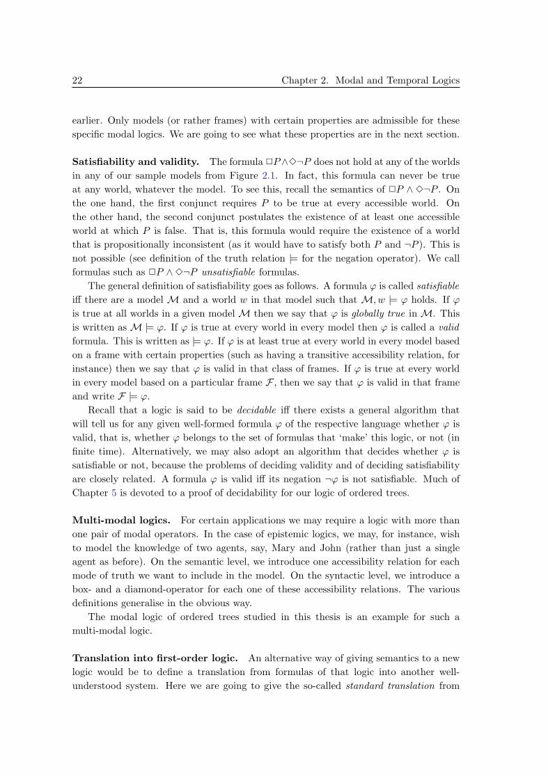
Satisfiability and validity. The formula 2P∧3¬P does not hold at any of the worldsin any of our sample models from Figure 2.1. In fact, this formula can never be trueat any world, whatever the model. To see this, recall the semantics of 2P ∧ 3¬P . Onthe one hand, the first conjunct requires P to be true at every accessible world. Onthe other hand, the second conjunct postulates the existence of at least one accessibleworld at which P is false. That is, this formula would require the existence of a worldthat is propositionally inconsistent (as it would have to satisfy both P and ¬P ). This isnot possible (see definition of the truth relation |= for the negation operator). We callformulas such as 2P ∧3¬P unsatisfiable formulas.
The general definition of satisfiability goes as follows. A formula ϕ is called satisfiableiff there are a model M and a world w in that model such that M, w |= ϕ holds. If ϕis true at all worlds in a given model M then we say that ϕ is globally true in M. Thisis written as M |= ϕ. If ϕ is true at every world in every model then ϕ is called a validformula. This is written as |= ϕ. If ϕ is at least true at every world in every model basedon a frame with certain properties (such as having a transitive accessibility relation, forinstance) then we say that ϕ is valid in that class of frames. If ϕ is true at every worldin every model based on a particular frame F , then we say that ϕ is valid in that frameand write F |= ϕ.
Recall that a logic is said to be decidable iff there exists a general algorithm thatwill tell us for any given well-formed formula ϕ of the respective language whether ϕ isvalid, that is, whether ϕ belongs to the set of formulas that ‘make’ this logic, or not (infinite time). Alternatively, we may also adopt an algorithm that decides whether ϕ issatisfiable or not, because the problems of deciding validity and of deciding satisfiabilityare closely related. A formula ϕ is valid iff its negation ¬ϕ is not satisfiable. Much ofChapter 5 is devoted to a proof of decidability for our logic of ordered trees.
Multi-modal logics. For certain applications we may require a logic with more thanone pair of modal operators. In the case of epistemic logics, we may, for instance, wishto model the knowledge of two agents, say, Mary and John (rather than just a singleagent as before). On the semantic level, we introduce one accessibility relation for eachmode of truth we want to include in the model. On the syntactic level, we introduce abox- and a diamond-operator for each one of these accessibility relations. The variousdefinitions generalise in the obvious way.
The modal logic of ordered trees studied in this thesis is an example for such amulti-modal logic.
Translation into first-order logic. An alternative way of giving semantics to a newlogic would be to define a translation from formulas of that logic into another well-understood system. Here we are going to give the so-called standard translation from

2.2 Possible World Semantics 23
general multi-modal logics into classical first-order logic. Such an embedding from onelogic into the other also shows that the basic (multi-)modal language cannot be moreexpressive than first-order logic. (This is a good thing, because otherwise we could nothope for decidability.)
Below we are going to give an inductive definition of a translation function st frommodal formulas to first-order formulas. Every propositional letter P of the modal lan-guage will be translated into a unary predicate P ′.6 For every pair of modal operators2R and 3R pertaining to an accessibility relation R we introduce a binary predicate R′.Every formula (with the exception of >) will be translated into a first-order formula witha single free variable. The name of that free variable appears as an index to the transla-tion function. For instance, we use stx to indicate that the resulting first-order formulawill have the free variable x. Intuitively, this variable stands for the worlds at whichthe modal logic counterpart of the first-order formula is true. The standard translationfunction is defined as follows:
stx(P ) = P ′(x) for propositional letters Pstx(>) = >
stx(¬ϕ) = ¬ stx(ϕ)stx(ϕ ∧ ψ) = stx(ϕ) ∧ stx(ψ)stx(3R ϕ) = (∃y)[R′(x, y) ∧ sty(ϕ)]stx(2R ϕ) = (∀y)[R′(x, y) → sty(ϕ)]
Here, each time we translate another diamond- or box-operator we have to choose a newbound variable y. The standard translation of modal formulas involving any of the otherpropositional connectives in the language may be inferred from the definitions of theseoperators in terms of negation and conjunction.
As an example, we translate the modal formula 2(P ∧ 3Q) into first-order logic.If we use the unary predicates P ′ and Q′ as translations of the propositional letters Pand Q, respectively, and if we use the binary predicate R′ to represent the accessibilityrelation underlying the pair of modal operators 2 and 3, using the standard translationwill yield the following result:
(∀y)[R′(x, y) → P ′(y) ∧ (∃z)[R′(y, z) ∧Q′(z)]]
Here, x is the free variable. Note that we have used a third variable name, namelyz, for the translation of the second modal operator appearing in the input formula.Alternatively, we could have reused the variable name x at this point. The resultingformula would then have been a first-order formula with only two distinct variable names(x and y). Inspection of the translation function st shows that, in fact, this is alwayspossible: any formula of the basic modal logic can be translated using at most two
6In order to clearly distinguish the language used for modal formulas from that of first-order logic,
we use letters with accents (such as P ′) to denote first-order predicate symbols. Of course, in practice
this would not be necessary.

24 Chapter 2. Modal and Temporal Logics
variable names. In other words, our basic modal logic can be embedded into the two-variable-fragment of first-order logic. The significance of this observation is that thetwo-variable-fragment is known to be decidable.7 Hence, the basic modal logic must bedecidable, too.
Our decidability proof for our modal logic of ordered trees given in Chapter 5 isalso based on the embedding into another system that is known to be decidable (in thiscase the second-order theory of two successor functions). A translation of our logic intofirst-order logic (over the theory of ordered trees) is given in Chapter 6.
2.3 Axioms and Correspondences
Axiomatic characterisation. In the previous section, we have seen how we can char-acterise the basic modal logic in terms of its model-theoretic semantics. Now we are goingto complement this view by giving an axiomatic (or proof-theoretical) characterisationof the same logic. An axiomatisation of a logic is a collection of axioms and inferencerules. The axioms are the basic formulas that are taken to be ‘true’ and the rules can beused to infer further such formulas. Formulas that can be derived in an axiomatic systemare called theorems of the system. A formula is called consistent iff it is not possible toderive its complement.
Intuitively, the concept of consistency corresponds to the semantic concept of satis-fiability, while the concept of theoremhood corresponds to semantic validity. Showingthat these concepts really coincide, that is, showing that the semantic and the axiomaticcharacterisation of a logic match can provide deep insights into either one of them. Wecall an axiomatisation sound (with respect to a given semantic characterisation) iff everysatisfiable formula is consistent. Dual to the concept of soundness is that of completeness.We call an axiomatisation (weakly) complete iff every consistent formula is satisfiable.8
Axioms and rules. Modal logic extends classical propositional logic. In particular,any formula that is a theorem of classical propositional logic (i.e. a tautology) will also bea theorem of the basic modal logic. Furthermore, any formula that we can construct byuniformly replacing propositional letters in a classical tautology by a well-formed formulawill be a theorem. For instance, ¬P ∨ P is a tautology and 3(ϕ ∧ ψ) is a well-formedmodal formula. Hence, the formula ¬3(ϕ ∧ ψ) ∨3(ϕ ∧ ψ) will be a theorem.
We are only going to give those axioms of the basic modal logic here that go beyondclassical logic. In fact, there are only two of them. The first one simply encodes theduality of the box- and the diamond-operator which we have already discussed earlier:
(Dual) 2A↔ ¬3¬A
7This was first shown by Scott in 1962 [63], for first-order logic without equality. Decidability of the
two-variable-fragment with equality is due to Mortimer [57] (see also [11]).8In Chapter 4 we also discuss the related concept of strong completeness (see page 106).
2.3 Axioms and Correspondences 25
That is, 2A↔ ¬3¬A is a theorem of the basic modal logic and so is any formula that wecan construct by substituting a well-formed formula for the letter A in this axiom. Thismatches our earlier definition of the semantics of the two modal operators. A formulasuch as A will be true in all accessible worlds iff it is not the case that it is not true insome accessible world.
While the duality axiom is essentially a definition of one modal operator in terms ofthe other, the second modal axiom really tells us something about the properties of ourmodal operators:
(K) 2(A→ B) → (2A→ 2B)
Axiom (K) is also known as the distribution axiom, because it expresses that we maydistribute the box-operator with respect to an implication.9 Again, we can easily verifythat this is a sound axiom: whenever A→ B is true in all accessible worlds and we thenfind that also A is true in all accessible worlds, we may conclude that the consequent Bmust be true in all accessible worlds as well.
There are three inference rules in the system. The first one is the rule of uniformsubstitution, which is familiar form classical propositional logic. It states that wheneverwe have derived a particular theorem we may uniformly substitute any one propositionalletter in that formula by an arbitrary well-formed formula of our modal language andwe obtain another theorem of the system. The second rule of inference is the well-known modus ponens, which says that whenever an implicational formula as well as itsantecedent are theorems, so is its consequent:
A, A→ B
B
The only strictly modal rule of the system is the so-called generalisation rule, whichis also known as the rule of necessitation, a reference to the alethic interpretation ofthe modal box-operator. The rule states that whenever a formula A is known to be atheorem then 2A will be a theorem as well:
A
2A
To see that this rule is semantically valid we make the following observation. If A is atheorem then A must be true at every world in any model. Hence, A will certainly betrue at all worlds accessible from some other world. But the latter is the truth conditionwe have used to semantically characterise the box-operator, i.e. 2A will also be true atany world in any model.
This axiomatic system is known to be complete with respect to the semantics definedin the previous section, that is, any formula for which we cannot derive its complementmust be a satisfiable formula. In other words, any formula that is valid can be derived.
9The name of the axiom (K) is generally understood to refer to Kripke, because it is characteristic
for the most basic modal logic that can be interpreted using Kripke models [45].

26 Chapter 2. Modal and Temporal Logics
We are not going to prove this result here. (A proof may, for instance, be found in [8].)Chapter 4 is devoted to these issues as far as our modal logic of ordered trees is concerned.It also outlines the general approach of obtaining completeness results by constructing aso-called canonical model.
Example. As an example, we demonstrate how the formula 3(A∨B) → 3A∨3B canbe derived from the axioms of the calculus just presented, that is, how it can be shown tobe a theorem. We first observe that it is easily seen to be semantically valid: wheneverthere is an accessible world in which either A or B is true then it will also be the case thatthere is either an accessible world satisfying A or there is an accessible world satisfyingB. Now let us see how we can get to the same result on the syntactic level. The proofsteps in the following derivation should be mostly self-explanatory. Some steps that doonly involve simple propositional reasoning are not carried out in full detail, but wecould easily fill in the missing bits. To begin with, we have to make a good guess whatinstantiation of an axiom or a propositional tautology may lead to the desired result.Here is our derivation:
(1) 2(¬A→ (¬B → ¬A ∧ ¬B)) → (2¬A→ 2(¬B → ¬A ∧ ¬B)) from (K)(2) ¬A→ (¬B → ¬A ∧ ¬B) propositional tautology(3) 2(¬A→ (¬B → ¬A ∧ ¬B)) from (2) by generalisation(4) 2¬A→ 2(¬B → ¬A ∧ ¬B) from (1) and (3)(5) 2(¬B → ¬A ∧ ¬B) → (2¬B → 2(¬A ∧ ¬B)) from (K)(6) 2¬A ∧2¬B → 2(¬A ∧ ¬B) from (4) and (5)(7) ¬2(¬A ∧ ¬B) → ¬2¬A ∨ ¬2¬B from (6)(8) 3¬(¬A ∧ ¬B) → 3A ∨3B from (7) and (Dual)(9) 3(A ∨B) → 3A ∨3B from (8)
In practice, axiomatic derivations can be difficult to find. One usually has to workbackwards, starting from the theorem to be derived.
Additional axioms for specific logics. As we have already observed in the previoussection, not all modal frames are suitable for reasoning about, say, knowledge. Similarly,not all formulas that are consistent with respect to the basic axiomatic system presentedin this section seem appropriate once we assign specific meaning to our modal operators.As an example, consider the formula 2P ∧ ¬P . This formula is consistent, because itsnegation is not derivable in our proof system.10 But do we want it to be consistent, forinstance, when working within an epistemic logic?
If we interpret the universal modality 2 as ‘Mary knows’, then our formula 2P ∧¬Preads: ‘Mary knows P but P is not true’. This is certainly not compatible with our
10This should be intuitively clear by inspection of the axioms and proof rules available to us (but a
truly formal argument why this is not possible is certainly more difficult). Going back to semantics, it is
very easy to see that 2P ∧ ¬P is also a satisfiable formula. All that is required is a model with a world
where P is false but true at every accessible world.

2.3 Axioms and Correspondences 27
understanding of the notion of knowledge. Anything that is known (by Mary or whomeverelse) in the true sense of the word must in fact be the case. We can integrate this ideainto our proof system by adding the following axiom:11
(T) 2A→ A
Postulating this axiom (for epistemic modal logics) means postulating veridicality ofMary’s knowledge: her knowledge accurately reflects the actual state of her environment.Given this additional axiom, 2P ∧¬P is easily seen to be inconsistent. Applying modusponens to 2P and a suitable instantiation of (T) yields P , which contradicts the secondconjunct ¬P . Axiom (T) is also desirable when reasoning about necessity. Surely,everything that is necessarily true will also be actually true. For doxastic logic, onthe other hand, the situation is different. Not every proposition believed to be true byJohn will in fact be true.
Next, let us consider the following axiom that may also arguably be added to ourproof system:12
(4) 2A→ 22A
In the context of reasoning about an agent’s knowledge, this axiom embodies the notionof positive introspection. It expresses that everything that is known must also be knownto be known. Axiom (4) also makes sense for the three other areas of application wehave discussed earlier. The alethic reading would be that whenever A is necessarily truethen this is necessarily the case. Under a doxastic interpretation, it states that what isbelieved is believed to be believed. Finally, in temporal logic, axiom (4) expresses thatwhenever A will be true always in the future, then also always in the future it will bethe case that always in the future A will be true.
In epistemic logic, related to positive introspection is the concept of negative intro-spection. We say that an agent is capable of performing a negative introspection of itsknowledge iff whenever it does not know about a proposition A then it does know thatit does not have this piece of knowledge. This property can be expressed by means ofthe formula ¬2A → 2¬2A. If we uniformly substitute A by ¬A in this formula andthen use the duality axiom to rewrite combinations of negation and the box-operator bydiamond-operators, we end up with the following (neater version of this) axiom:13
(5) 3A→ 23A
The concept of negative introspection is not generally accepted as a property of knowl-edge. That is, there are epistemic logics that include axiom (5) and there are others thatdo not include it. Being aware of what one does not know (as in the case of negative
11The name of axiom (T) goes back to the work of Feys [21, 22] who first described a logical system
(“la logique t”) centred around this axiom (quoted after [15]).12The name of this axiom is a reference to the work of Lewis [49]. Axiom (4) is the characteristic
axiom in S4, the fourth of his logical systems of strict implication.13Axiom (5) is characteristic for S5, Lewis’ fifth system of strict implication; hence the name [49].

28 Chapter 2. Modal and Temporal Logics
introspection) arguably requires a higher state of consciousness than merely being awareof what one does know (as for positive introspection). In the case of belief, i.e. for dox-astic logics, the situation is less critical. If John does not believe in the truth of A thenhe can be expected to also believe that he does not believe in A.
For alethic logic, axiom (5) seems reasonably acceptable: if something is possiblytrue then this is necessarily so. For temporal logic, however, we clearly have to rejectaxiom (5). It is not the case that, if A will be true at some point in the future, then thiswill remain so forever.
We have mentioned on more than one occasion that the notion of belief is weaker thanthat of knowledge, in the sense that what is believed is not necessarily required to betrue. Nevertheless, a rational agent will not believe just about anything. In particular,it seems reasonable to postulate that a rational agent would not believe in a propositionthat is logically inconsistent. In this case, we should adopt the formula ¬2⊥ as an axiom.The same is true for both alethic and epistemic logics: what is inconsistent can hardlybe necessarily true or ‘known’ to be true by a rational agent. Exploiting the duality of2 and 3, we can rewrite the formula ¬2⊥ as follows:14
(D) 3>
The temporal interpretation of (D) is clear: it embodies the concept of an endless future;for any point in time there always still exists a later point. Time never stops. Thiswill be a useful assumption for most applications, but whether or not to adopt it ina particular situation is, as ever, entirely up to the logic engineer devising the formalsystem in question.
Naming conventions for standard modal logics. The axioms we have introducedin this section form the basis of some of the most important systems of basic modallogic. The logic determined by axiom (K), together with the duality axiom and the setof all classical tautologies as well as modus ponens, the generalisation rule, and the ruleof uniform substitution is known under the name of K. This is the logic we have so farreferred to as ‘the’ basic modal logic. The names of other logical systems can be derivedby appending the letters (or numbers) referring to the chosen additional axioms at theend of the name of a logic. For instance, the logic KT4 is the modal logic we get byadding axioms (T) and (4) to the basic calculus of K. Besides this systematic namingscheme, also a number of rather more traditional names are being used for particularbasic modal logic systems. The logic KT4, for instance, is usually referred to as S4,while KT5 is better known as S5. These are the original names of Lewis’ systems ofstrict implications [49].
It follows from our discussion of the various additional axioms presented here, that S5is a system that is appropriate for reasoning about alethic modes of truth,15 while KD45
14The name of axiom (D) stems from its central role in deontic logic, another important branch of
modal logics. Deontic logics are used to formalise concepts such as obligation and permission [3].15Axioms (D) and (4) are derivable in S5.

2.3 Axioms and Correspondences 29
is an example for a doxastic logic. Both S4 and S5 may serve as epistemic logics thatallow us to model the knowledge of a single agent (the latter only if we are prepared toaccept negative introspection). However, no combination of the simple axioms presentedhere seems to be strong enough to adequately characterise a system of temporal logic.
Indeed, axiomatising temporal logics is typically more difficult than axiomatisingvarious other systems of modal logic. Chapter 4 addresses some of the issues involved inthe context of our extended temporal logic based on ordered trees.
Correspondence theory. As we have just seen, the axiomatic approach can be veryhelpful in making certain characteristics of modalities, such as veridicality or positiveintrospection in the case of an epistemic interpretation, precise. On the other hand,the semantic view often provides the better intuitions when we think about what istrue, can be true, or must be true. For instance, it is usually more convenient to thinkabout satisfiability and the existence of models rather than consistency and the lackof axiomatic derivations. To bring these two perspectives on modal logic together onceagain, in the remainder of this section, we shall discuss the question of how the additionalaxioms introduced earlier are reflected in the structure of the corresponding models.
As we shall see, each one of them, in fact, corresponds to a simple (and intuitive)property of the underlying accessibility relation. This object of study in modal logics isknown as correspondence theory [69].
The case of reflexive frames. Axiom (T), for instance, which we have introducedearlier, characterises the class of reflexive frames, i.e. frames with a reflexive accessibilityrelation. Recall that (T) stands for the formula 2A → A. By saying that this formulacharacterises the class of reflexive frames we mean, more concretely, the following:
Claim: Let F = (W,R) be a frame. Then (T) is valid in F iff R is reflexive.
How can we prove such a correspondence result? Showing that reflexivity of the acces-sibility relation associated with a particular frame implies validity of (T) in that frameis the easier part. In short, we have to verify that 2A→ A is true at every world in anymodel based on a reflexive frame. So let F = (W,R) be a frame with a reflexive accessi-bility relation R. By definition of the notion of frame validity, showing that 2A→ A isvalid in F amounts to showing that M, w |= 2A→ A holds for every model M = (F , V )based on the frame F and every world w ∈W . So let M = (F , V ) be an arbitrary modelbased on F and let w be an arbitrary world in W . To prove that M, w |= 2A → A
holds, we assume M, w |= 2A and try to infer M, w |= A. The former is the case iffM, w′ |= A holds for all w′ ∈ W with (w,w′) ∈ R. This is where our premise of thereflexivity of the accessibility relation comes into play. Given that R is reflexive, we have(w,w) ∈ R, i.e. M, w |= A must hold. That is, we have shown that 2A→ A will be truein any model M based on the frame F and at any world w in that frame. Hence, (T) isvalid in F as claimed.

30 Chapter 2. Modal and Temporal Logics
Axiom Frame Condition
(T) 2A→ A (∀x)R(x, x) (reflexive)(B) A→ 23A (∀x)(∀y)[R(x, y) → R(y, x)] (symmetric)(4) 2A→ 22A (∀x)(∀y)(∀z)[R(x, y) ∧R(y, z) → R(x, z)] (transitive)(5) 3A→ 23A (∀x)(∀y)(∀z)[R(x, y) ∧R(x, z) → R(y, z)] (euclidean)(D) 3> (∀x)(∃y)R(x, y) (serial)
Table 2.2: Basic correspondences
Now for the other direction. Suppose (T) is valid in the frame F = (W,R), i.e.2A → A is true in every model based on F at every world in the frame. We need toshow that R must be a reflexive relation. For the sake of contradiction, assume this isnot the case, i.e. there exists a world w ∈ W such that (w,w) 6∈ R. We are going touse this world w to define a valuation function V such that 2A → A is not satisfiedat w in the model M = (F , V ). In fact, all we need to specify about V is what setof worlds it maps the propositional letter A to. Let V be any valuation function suchthat V (A) = W \ w and let M = (F , V ) be the corresponding model. It follows thatM, w |= 2A holds, because A is satisfied at every world accessible from w (given thatw itself, the only world where A is false, is not accessible), and that M, w |= A doesnot hold. Hence, M, w |= 2A→ A is not the case either, which contradicts our originalassumption of (T) being valid in F . This completes our proof of the above claim.
Other correspondences. Similarly to the reflexivity axiom (T), each one of the ad-ditional axioms we have discussed earlier also corresponds to a simple frame condition.These correspondences are summarised in Table 2.2 and can be proved to hold in essen-tially the same manner as we have verified the correspondence between (T) and the classof reflexive frames. The table also shows how the respective frame conditions can beexpressed in first-order logic. The formula (∀x)R(x, x), for example, defines the relationassociated with the binary predicate symbol R as being reflexive.
Axiom (4) characterises transitive frames and axiom (5) characterises those that havea euclidean accessibility relation, i.e. frames where it is the case that whenever two worldsare accessible from the same world then those two worlds must be accessible from eachother as well. Axiom (D) is valid in frames where every world has at least one successorwith respect to the accessibility relation; that is, (D) embodies the notion of seriality. Inaddition to the axioms discussed earlier, Table 2.2 also lists another important schema:16
(B) A→ 23A
This formula may, for instance, be adopted as an axiom of alethic logic, in which case itexpresses that anything that is true in the actual world is necessarily possible. It is validin a frame iff that frame has got an accessibility relation that is symmetric.
16It appears that axiom (B) was first proposed by Becker [7], who referred to it as the “Brouwersche
Axiom” (quoted after [49]; see also [15]).

2.4 Temporal Logic 31
In the context of our ordered tree logics, we are briefly going to discuss issues incorrespondence theory in Chapter 3 (Section 3.3).
First-order definability. Our presentation may suggest that any modal axiom wecan think of characterises a frame condition that can be defined in terms of a first-orderformula over the predicate R representing the accessibility relation. This is in fact notthe case. The best known counterexample is the so-called McKinsey axiom:17
(M) 23A→ 32A
It can be shown that (M) does not correspond to any first-order frame condition. Aproof may, for instance, be found in [69].
Translation again. As a final remark in this section let us point out that in those caseswhere a modal logic is first-order definable, the respective first-order frame conditionsmust be taken into account if we want to embed that modal logic into first-order logic(by means of translation). The logic S4, for example, — which is characterised by theadditional axioms (T) and (4) — cannot be embedded into the two-variable-fragment offirst-order logic anymore, because we require a minimum of three distinct variable namesto encode the transitivity condition corresponding to (4). Hence, the argument used atthe end of the previous section to show that the basic modal logic without any additionalaxioms (i.e. the logic K) is decidable, would fail in this case.18
This concludes our general introduction to basic modal logic. The next section ismore specifically devoted to the case of temporal logic.
2.4 Temporal Logic
Temporal modal logics are modal logics over very specific frames that embody thoseaspects of time we wish (and are able) to represent.
What is time? This is a (largely philosophical) question, which we are not going toanswer here. Instead, we are going to be rather more pragmatic and discuss some ofour options as far as representing aspects of time by means of a modal logic frame areconcerned. Recall that a frame consists of a set of worlds together with an accessibilityrelation (or several accessibility relations in the case of multi-modal logics). If we wantto give such a frame a temporal interpretation, we first have to decide what worlds andaccessibility relation(s) should stand for. Generally speaking, worlds will be used torepresent the primitive objects in the domain of our temporal semantics. In most cases,that is, for most temporal logics discussed in the literature, these primitive objects aretime points. Alternatively, we may also choose time intervals as primitives.
17Axiom (M) is called the McKinsey axiom, because it is a theorem in the system S4.1 proposed by
McKinsey in [55] (see also [42]).18S4 is still a decidable logic, but we require a different method to prove this [8].

32 Chapter 2. Modal and Temporal Logics
In the case of a point-based semantics, the accessibility relation induces an earlier-later ordering over time points. An example would be the temporal frame (N0, <),where the set of points (worlds) is the set of the natural numbers (including 0) and theaccessibility relation < is the usual lower-greater ordering over N0. By adopting thisframe, we are making certain assumption about time: it is discrete (in particular, forevery point in time there is a unique next point), bounded to the left, namely by thefirst time point 0 (the ‘big bang’, the beginning of time), and unbounded to the right(i.e. the future is taken to be without end). None of these choices is obligatory though.In particular, we may consider temporal frames that are dense (if the notion of a ‘next’moment is inappropriate for an application) or unbounded to the left (if we want tomodel both future and past). More fundamentally, in the case of the frame (N0, <), timeis understood to be linear. But again, this is not an obligatory choice. For instance, ifwe wish to explicitly represent different possible futures, we may adopt a temporal framewhere time is branching. However, for the remainder of this introduction (the remainderof this thesis, in fact) we are going to assume that time is linear.19
If we choose intervals as primitives, then a single accessibility relation representing asimple earlier-later ordering (possibly together with the notion of alternative futures, inthe case of branching time) will not be enough anymore. Two distinct intervals may notonly lie either before or after each other, but for instance, one of them may also occurduring the other or they may overlap. While in this introduction, we are only going to beconcerned with point-based temporal logics, our modal logic of ordered trees discussedin the rest of this thesis may also be interpreted as a (restricted) interval logic.20
Temporal logic operators. The language of the most basic temporal logics is thesame as the basic modal language introduced earlier. Besides the propositional connec-tives, we have a box-operator 2 to refer to all future points in time and a diamond-operator 3 to refer to some future point. In addition to that, temporal logics oftenalso include a so-called next-operator e to refer to the time point immediately after thecurrent one. If we also wish to speak about events that happened in the past, we maychoose a logic with two sets of operators, one for the future and the other one for thepast. We are going to use the symbols 2, 3, and e to denote future operators and 2,3, and e for past operators.
An even more expressive temporal logic may also include the additional operatorssince and until. Intuitively, the formula (ϕ until ψ) is true now iff ψ is true at somepoint in the future and ϕ is true until that point in time. The operator since serves asimilar purpose with respect to past events. To be able to give a precise definition ofthe meaning of these and the other operators, we first have to decide on a particularsemantics for our temporal logic. In what follows, we shall discuss propositional lineartemporal logics over various flows of (linear) time.
19An overview of branching time logics (as well as references to further reading) may be found in [33].20On this point, consult in particular our discussion on pages 45 and 189.

2.4 Temporal Logic 33
Semantics of propositional linear temporal logics. A linear temporal logic frameis a strict linear order F = (T,<).21 The set T is called the set of states (or timepoints) and the relation < represents the temporal order declared over these states. Atemporal frame is a special case of a modal frame: T takes the role of the set of worlds,which we have previously denoted by W , and < is a particular kind of accessibilityrelation, which we have used the letter R for in the general case. A model is again apair M = (F , V ), where F = (T,<) is a temporal frame and V is a valuation functionmapping propositional letters to sets of states in the frame. The truth of a temporalformula at a state t ∈ T in a model M is now defined as follows:22
(1) M, t |= P iff t ∈ V (P ) for propositional letters P ;
(2) M, t |= >;
(3) M, t |= ¬ϕ iff M, t 6|= ϕ;
(4) M, t |= ϕ ∧ ψ iff M, t |= ϕ and M, t |= ψ;
(5) M, t |= 3ϕ iff there exists a t′ ∈ T such that t < t′ and M, t′ |= ϕ;
(6) M, t |= 2ϕ iff for all t′ ∈ T with t < t′ we have M, t′ |= ϕ;
(7) M, t |= eϕ iff t has an immediate successor t′ ∈ T and M, t′ |= ϕ;
(8) M, t |= ϕ until ψ iff there exists a t′ ∈ T with t < t′ and M, t′ |= ψ, andfurthermore M, t′′ |= ϕ holds for all t′′ ∈ T with t < t′′ and t′′ < t′.
The semantics of the past operators are defined in direct analogy to the above. Forinstance, we have M, t |= ϕ since ψ iff there is a t′ ∈ T with t′ < t and M, t′ |= ψ, andϕ holds at all states t′′ in between that t′ and t. The notions of satisfiability and validityof a temporal logic formula are defined in analogy to the general case discussed earlier.
Instead of a general linear order (T,<) we may also choose to work with a specific flowof time, such as the natural numbers (N0, <) or the reals (R, <), or we may put at leastsome additional constraints on (T,<), such as being dense, discrete, or unbounded toeither side. These choices influence what formulas are going to be valid in the respectivelogic. For instance, a formula of the form eϕ will never be true at any state if we choose(R, <) as the underlying flow of time, because no real number has got an immediatesuccessor.
Definable operators. Rather than defining the semantics of the two box-operators ofthe temporal language directly (as we have done here), we may also choose to treat themas defined operators. As we have seen earlier, a box-operator can be defined in terms ofnegation and the corresponding diamond-operator:
2ϕ = ¬3¬ϕ 2ϕ = ¬3¬ϕ21Strict linear orders are defined in Appendix A.22Propositional connectives other than negation and conjunction are again treated as defined operators.

34 Chapter 2. Modal and Temporal Logics
In fact, now that we have enriched our language with the operators since and until,both diamond- and next-operators may also be treated as defined operators:
3ϕ = > until ϕ eϕ = ⊥ until ϕ
3ϕ = > since ϕ eϕ = ⊥ since ϕ
These syntactic definitions are easily seen to coincide with the semantic truth conditionsgiven earlier. For instance, the first part of the semantic definition of truth for theformula (> until ϕ) postulates the existence of a future time point at which ϕ holds— this is precisely how we have defined the truth of 3ϕ. To understand the syntacticdefinition of the next-operators, consider the meaning of the formula (⊥ until ϕ). Wehave M, t |= ⊥ until ϕ iff, to begin with, there exists a state t′ such that t < t′ andM, t′ |= ϕ. The second part of the truth condition says that ⊥ must be true a everystate that lies strictly between t and t′. But ⊥ can never be true, i.e. there cannot be anystates between t and t′. Hence, t′ must be the immediate successor of t and M, t |= eϕwill hold.
Expressive completeness. Our discussion shows that we can reduce the set of con-nectives to four core operators: negation, conjunction, since and until. They form afunctionally complete set of operators with respect to our chosen temporal language, thatis, all of the other operators we have discussed here are definable in terms of these four. Inclassical propositional logic, we know that negation and conjunction form a functionallycomplete set of operators, not only with respect to the usual language of propositionallogic (which includes, for instance, the disjunction and the implication operators), butalso with respect to the logic itself. That is, it is not possible to even conceive an addi-tional operator that is not expressible in terms of negation and conjunction alone. Thisis a direct consequence of the simple observation that negation and conjunction sufficeto uniquely identify any row in a truth table.
Is there a similar phenomenon in temporal logic? Defining the notion of functionalcompleteness for classical propositional logic is straightforward. Propositional logic istruth-functional, that is, a set of operators is functionally complete iff it can be usedto encode every possible function over a finite number of truth values. As for temporallogic, a suitable definition of functional completeness (pertaining to the semantics ofthe logic rather than a particular language) is not that immediate. What would bea suitable benchmark, that is, how can we measure the expressive power of a set oftemporal operators? At this point, let us recall the standard translation of modal logicsinto classical first-order logic discussed in Section 2.2. If we use < as the binary predicatesymbol representing the accessibility relation, then the formula (ϕ until ψ) translatesinto the following first-order formula (with a free variable x):
(∃z)[x < z ∧ stz(ψ) ∧ (∀y)(x < y ∧ y < z → sty(ϕ))]
Here, sty(ϕ) and stz(ψ) represent the translations of the subformulas ϕ and ψ. Thetranslation of formulas involving other operators works accordingly. That is, the trans-

2.4 Temporal Logic 35
lation of any temporal logic formula will always be a first-order formula with one freevariable, a single binary predicate symbol < together with a number of unary predicatesymbols (representing the propositional letters in the input formula), and no constantor function symbols. Furthermore, < has a fixed intended meaning, namely the earlier-later ordering over the chosen flow of time. In other words, temporal logic formulas arebeing translated into the monadic first-order theory of a particular linear order. Now thequestion whether we can always translate any formula of that theory back into temporallogic provides a useful yardstick for the expressive power of a temporal logic.
A set of operators of a temporal logic is called expressively complete with respect toa certain flow of time (T,<) iff for every formula ϕ∗ of the monadic first-order theoryof (T,<) there is a formula ϕ of the temporal logic such that the standard translationof ϕ is logically equivalent to ϕ∗. The concept of expressive completeness for temporallogics has been introduced by Kamp in 1968 [44]. His main result was that since anduntil (together with the connectives for negation and conjunction) are expressivelycomplete for linear orders (T,<) that are complete, i.e. where every non-empty boundedsubset of T has both a greatest lower bound and a least upper bound with respect to<. This includes, in particular, the temporal frames (N0, <) and (R, <), but not, forinstance, (Q, <). For arbitrary linear flows of time additional operators — the so-calledStavi connectives — are required to obtain expressive completeness [32]. The subject ofexpressive completeness is comprehensively treated in the monograph on temporal logicby Gabbay, Hodkinson, and Reynolds [30].
We shall briefly comment on issues related to expressive completeness for our modallogic of ordered trees in Chapter 6.
Temporal logic and specification. The application of temporal logics in the area ofsystems specification and verification is one of the great success stories of non-classicallogics in mainstream computer science. In fact, in recent years, writing temporal logicbased specifications and developing tools for their verification have become engineeringdisciplines in their own right. In a theoretical text such as this we can only hope, atbest, to convey some of the basic ideas by means of example.
If we think of a system as a sequence of states in which certain basic propositions (say,a variable having a certain value or a certain event occurring) are either true or false, thenwe can identify such a system with a linear temporal logic model. A specification may bethought of as a list of properties that we would like our system to have. Two importantclasses of program properties — that arguably cover most properties one could wish toinclude into a system specification — are the so-called safety and liveness properties,which have been characterised by Lamport [47] as follows:
• Safety properties “assert that the program does not do something bad”.
• Liveness properties “assert that the program does eventually do something good”.
The latter immediately reminds us of the temporal diamond-operator: at some point in

36 Chapter 2. Modal and Temporal Logics
the future something good is going to happen. The former is reminiscent of the box-operator: always in the future it is not the case that things get pear-shaped. That is, asafety property can typically be expressed by a formula of the form 2¬Bad, where Badis itself a temporal formula, while a liveness property will often be of the form 3Good.Such formulas may or may not be true at (all) the states of the model representing asystem, that is, such a system may or may not conform to its specification.
Examples. We conclude with a number of examples for simple specification formulastaken form a variety of sources [30, 51]. For these examples, we do not assume anyspecific flow of time. Our only requirement is that there is a first point in time andthat time is not bounded to the right. The specified system has a particular property iffthe corresponding formula is true at the first state in the model representing the system.Many of these formulas start with the box-operator 2 to express that a particular formulais supposed to be true at every state of the system.
• Mutual exclusion. Two processes A and B are never going to be in their criticalsections of execution at the same time:
2¬(CriticalA ∧ CriticalB)
• Partial correctness. After computation has finished a given postcondition will hold:
2(Finished → PostCondition)
• Termination and total correctness. Partial correctness together with terminationyields the property of total correctness:
3Finished ∧ 2(Finished → PostCondition)
• Response to an impulse. Whenever the system receives a particular impulse thenit will eventually respond appropriately:
2(Trigger → 3Response)
• Absence of unsolicited response. If at some point during program execution thesystem performs a certain action, then that action must have been triggered by theappropriate event:
3Action → (¬Action until Trigger)
This action may, for instance, be thought of as the system response from theprevious example.
• Unique events. A particular event may happen at most once, that is, whenever itdoes happen it must be the case that it did not happened earlier as well:
2(Event → 2¬Event)

2.5 Bibliographic Notes 37
2.5 Bibliographic Notes
The aim of this chapter has been to introduce some of the fundamental concepts ofthe study of modal and temporal logics and to indicate how they relate to the originalwork reported in the remainder of this thesis. Our choice of topics has been somewhatselective. Important omissions include, for instance, the whole area of deduction [4, 25,59, 73] and particularly model checking [17, 18], first-order modal logics [26, 34, 42], andcombinations of modal systems [31, 53].
Literature. The brief survey by van Benthem [70] is a very readable introductionto the field of modal logics and the forthcoming handbook chapter by Goldblatt [36]provides an extensive review of its history. Recommendable textbooks on modal logicin general include, for instance, those by Hughes and Cresswell [42], Chagrov and Za-kharyaschev [13], and Blackburn, de Rijke, and Venema [8]. The latter, in particular,has proved to be an extremely useful guide throughout the preparation of this thesis.Another indispensable source of information on modal logic in general and temporal (anddynamic) logics in particular is the excellent book by Goldblatt [35]. An important bookdevoted specifically to the study of temporal logics is the work by Gabbay, Hodkinson,and Reynolds [30] (see also the second volume [33]).
Throughout this chapter we have borrowed from the area of modal logics of knowledgeand belief, because they are particularly well suited to exemplify issues such as theneed for different sets of axioms for different applications. We are not going to furthercontinue this theme here and instead refer to the book by Fagin et al. [20] (and referencestherein) for more information on the subject. The book by Huth and Ryan [43] is arecent textbook focussing on the use of logic (and notably modal and temporal logics)in different areas of computer science. It discusses, in particular, epistemic logics formulti-agent systems and temporal logic model checking for specification and verification.The area of temporal logic specification is also treated in great breadth as well as depthin the two books on the subject by Manna and Pnueli [51, 52].
Conclusion. This concludes our general exposition of elementary modal and temporallogics. In the next chapter we are going to return to our main object of investigation,the modal logic of ordered trees.

Chapter 3
Semantic Characterisation
This chapter is mostly concerned with a semantic (as opposed to axiomatic) characteri-sation of our modal logic of ordered trees. We start with a formal definition of its syntaxand model-theoretic semantics. After that, we are going to give a number of examplesthat demonstrate the expressive power of ordered tree logics. For instance, powerfuloperators such as the universal modality turn out to be definable within our logic. Weare also going to discuss a number of correspondence results, which show that the logic isexpressive enough to distinguish different classes of ordered trees (such as finite trees, forexample). Thereafter, we are going to show how we can characterise different ontologicalcategories of propositions. This allows us, for instance, to distinguish so-called proper-ties from events, which are notions commonly referred to in the literature on planningin artificial intelligence.
In our logic, frames are required to be ordered trees. Towards the end of this chapterwe investigate to what extent we can relax the conditions on frames without changingthe logic (that is, without changing the set of formulas that are satisfiable with respectto these frames). For this investigation we are going to make heavy use of the conceptof p-morphic images of frames.
3.1 Syntax and Semantics
In this section we are going to give formal definitions of the syntax and semantics of themodal logic of ordered trees we have already introduced informally in Chapter 1. Weshall refer to this logic as OTL, for ordered tree logic.
Syntax. We start by defining the syntax of well-formed formulas of OTL. The lan-guage is built around a countable set of propositional letters (such as P orQ) and complexformulas can be formed by combining simpler formulas by means of a number of logicaloperators.
Definition 3.1 (Formulas) The set of well-formed formulas of OTL is the smallestset such that propositional letters and the symbols > and ⊥ are formulas and, if ϕ and
39

40 Chapter 3. Semantic Characterisation
ψ are formulas, so are (¬ϕ), (ϕ ∧ ψ), (ϕ ∨ ψ), (ϕ → ψ), (ϕ ↔ ψ), ( eϕ), (3ϕ), (2ϕ),( eϕ), (3ϕ), (2ϕ), ( eϕ), (3ϕ), (2ϕ), (3ϕ), (2ϕ), (3+ϕ), and (2+ϕ).
The symbols > (verum) and ⊥ (falsum) as well as the connectives ¬ (negation), ∧(conjunction), ∨ (disjunction), → (implication), and ↔ (if-and-only-if) are familiar frompropositional logic. As for the modal operators, we distinguish next-operators ( e, e, e),diamond-operators (3, 3, 3, 3, 3+), and box-operators (2, 2, 2, 2, 2+). Followingstandard convention, we are usually going to avoid redundant brackets when writingformulas.
Semantics. The semantics of formulas in OTL will be given by means of a definitionof the notion of truth of a formula in a model. Models are based on ordered trees, i.e.the frames for this modal logic are ordered trees.
Ordered trees. An ordered tree is a tree where the children of each node are ordered.We use standard terminology when speaking about trees. In particular, we shall refer tothe parent of a node (the node directly above a given node) and the children of a node(the nodes directly below a given node). The set of ancestors of a node includes thatnode’s parent, the parent’s parent, and so forth. Similarly, the descendants of a nodeare all the nodes on the branches below that node. Nodes sharing the same parent arecalled siblings. As we are working with ordered trees, we shall distinguish siblings to theleft and siblings to the right of a given node. Finally, a node can have a left and a rightneighbour, that is, a sibling coming directly before or after, respectively, in the orderdeclared over that particular set of siblings.
Branches may be of finite or infinite length. Also, a node may have a finite or aninfinite number of children. A node does not necessarily have to have a first or a lastchild; there could be infinitely many siblings in either direction. Also, we do not requirethe order declared over the children of a node to be, say, discrete. Instead, we admitany kind of linear order. (Discrete or dense linear orders may, however, be considered asinteresting special cases.)
Next we are going to formally define the notion of ordered tree. However, later on wewill often find it more convenient to refer to the intuitive notions introduced before. Thefollowing definition of a tree is a slight modification of that given by Goldblatt in [35].1
Definition 3.2 (Trees) A tree is a pair T = (T,R), where T is a set and R is anirreflexive binary relation over T satisfying the following conditions:
(1) For every t ∈ T there exists at most one t′ ∈ T with (t′, t) ∈ R.
1Here and in the sequel we are going to refer to a number of relational algebra operations. The inverse
of a relation R is denoted by R−1. The composition of two relations R1 and R2 is written as R1 R2.
Given a relation R, let R∗ denote the reflexive transitive closure of R and R+ the non-reflexive transitive
closure of R, respectively. (See also Appendix A.)

3.1 Syntax and Semantics 41
(2) There exists a unique r ∈ T such that t ∈ T | (r, t) ∈ R∗ = T .
The elements of T are called nodes. The element r from condition (2) is called the rootof T . R is called the child relation and also gives rise to the following: the parent relationR−1, the descendant relation R+, the ancestor relation (R−1)+, and the sibling relationR−1R.
So by referring, for instance, to a node t1 as the parent of t2, we mean that (t1, t2) ∈ R.Node t2 is then called a child of t1. Similarly, if (t1, t2) ∈ R+ then t1 is called an ancestorof t2, and t2 is called a descendant of t1. Two nodes that share the same parent are calledsiblings. Starting at any node, if we first move up one level using the parent relation(that is, the inverse of the child relation) and then one level down via the child relation,we will end up at a sibling of the first node. In other words, if we have (t1, t2) ∈ R−1Rthen t1 is called a sibling of t2 and vice versa. Nodes that do not have any children atall are called leaves. All other nodes of a tree are called internal nodes.
The nodes in a tree (the kind of tree characterised through Definition 3.2) may beconsidered as being ‘generated’ by the root node via the transitive closure of the childrelation R. This excludes certain kinds of structures, such as trees (in a wider sense ofthe word) where the child relation could, for instance, be dense. In other words, we onlyconsider trees of order-type N, that is, any branch could be mapped to an initial segmentof the natural numbers. It follows that the length of a branch will be either finite orcountably infinite.
The following is a formal definition of the notions of branch and subtree. Here (andthroughout) we write (T ′, R), where R is a binary relation declared over some supersetT of T ′, rather than explicitly restricting R to range only over T ′.
Definition 3.3 (Branches and subtrees) Let T = (T,R) be a tree and t ∈ T a nodewithin T . We refer to the set t′ ∈ T | (t′, t) ∈ R∗ as (the nodes on) the branch above tand to the tree (t′ ∈ T | (t, t′) ∈ R∗, R) as the subtree generated by t.
We are now ready to define ordered trees as trees with an additional (linear) order overthe nodes. Observe that the sibling relation R−1 R is an equivalence relation overthe set of nodes excluding the root. For a given node t the ‘quasi-equivalence class’[t]R−1R = t′ ∈ T | (t, t′) ∈ R−1R is the set of siblings of t (including t itself); only ift is the root of the tree then [t]R−1R is the empty set.
Definition 3.4 (Ordered trees) An ordered tree is a triple T = (T,R, S) where (T,R)is a tree, S ⊆ R−1R, and ([t]R−1R, S) is a strict linear order for every t ∈ T .
If (t1, t2) ∈ S then t1 is called a left sibling of t2, and t2 is called a right sibling of t1.If furthermore (t1, t2) 6∈ S S then t1 is called the left neighbour of t2, and t2 is calledthe right neighbour of t1.
When referring to a node t in a tree T we will occasionally write t ∈ T instead of explicitlyintroducing the set of nodes T (i.e. instead of writing t ∈ T with T = (T,R, S)).

42 Chapter 3. Semantic Characterisation
•root
•P1, P2 • •P1
•P2, P3
• • • • • •P1
• • •P2
• •
• •P1
•P1, P2
• • • • • •P1
ww ''// // //
// //
// yy %%// // // // //
// //
// // //
//
Figure 3.1: A simple ordered tree model
We will sometimes write ≺ for the child relation R and < for the sibling order S.As before, ≺∗ and ≺+ refer to the reflexive and the non-reflexive transitive closure of ≺,respectively. We also write t1 ≤ t2 as an abbreviation for t1 < t2 or t1 = t2.
According to our definition of ordered trees, the horizontal relation declared over thechildren of a given node could be any strict linear order. In particular, it is not requiredto be discrete. This means, for example, that it is possible that a node has righthandsiblings but no righthand neighbour, namely when that node is dense, i.e. when there areinfinitely many nodes between itself and any of its righthand siblings. In other words,our logic is going to be an extension of linear temporal logics over general flows of time.
Models. We can now move on to the definition of models and the notion of truth offormulas in models for our logic OTL. Frames in this modal logic are ordered trees.
Definition 3.5 (Ordered tree models) An ordered tree model is a pair M = (T , V ),where T is an ordered tree and V is a valuation, that is, a mapping from propositionalletters to subsets of the set of nodes in T .
When speaking about models, we will sometimes simply write M = (T,R, S, V ) as ashorthand for M = (T , V ) with T = (T,R, S).
Figure 3.1 shows a simple example of an ordered tree model.2 In the picture, thechild relation R is shown as a dotted line, while the right neighbour relation S \ S Sis drawn as a solid line. The valuation function V is indicated by writing propositionalletters (in the example these are P1, P2 and P3) next to the respective nodes. The set
2In this particular example every node has got a finite number of children and, consequently, the order
declared over sibling nodes must be discrete. However, this need not be the case in general.
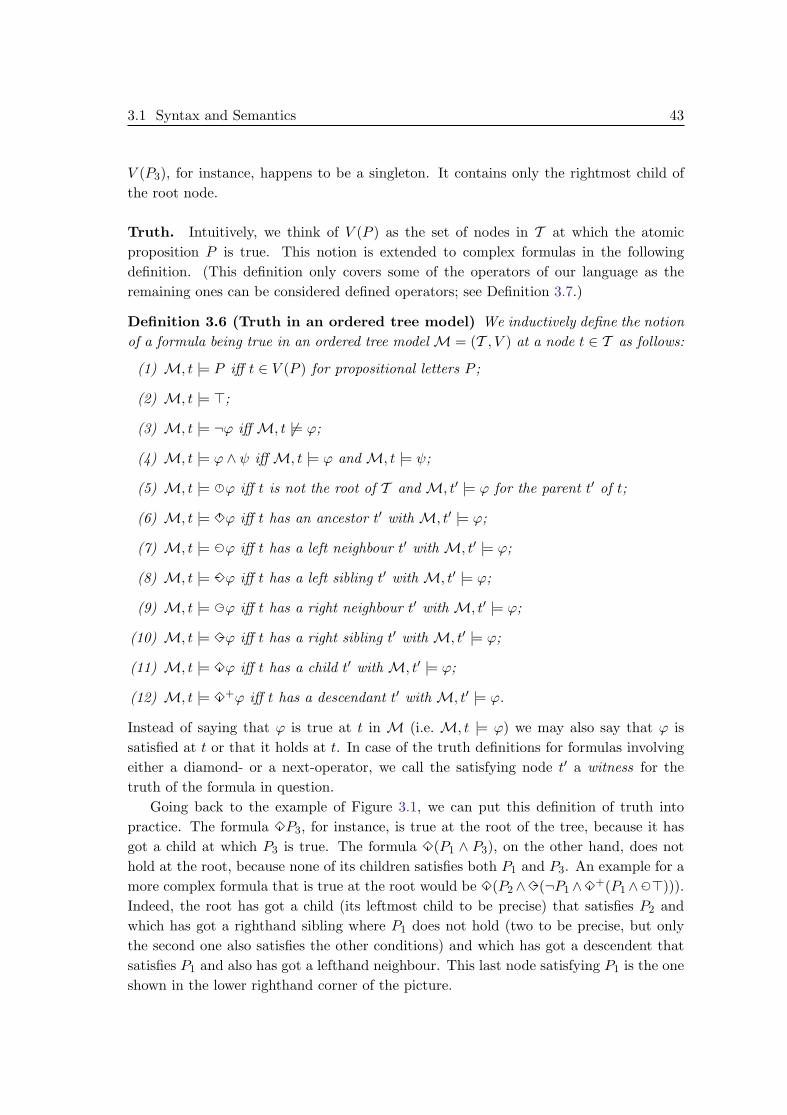
3.1 Syntax and Semantics 43
V (P3), for instance, happens to be a singleton. It contains only the rightmost child ofthe root node.
Truth. Intuitively, we think of V (P ) as the set of nodes in T at which the atomicproposition P is true. This notion is extended to complex formulas in the followingdefinition. (This definition only covers some of the operators of our language as theremaining ones can be considered defined operators; see Definition 3.7.)
Definition 3.6 (Truth in an ordered tree model) We inductively define the notionof a formula being true in an ordered tree model M = (T , V ) at a node t ∈ T as follows:
(1) M, t |= P iff t ∈ V (P ) for propositional letters P ;
(2) M, t |= >;
(3) M, t |= ¬ϕ iff M, t 6|= ϕ;
(4) M, t |= ϕ ∧ ψ iff M, t |= ϕ and M, t |= ψ;
(5) M, t |= eϕ iff t is not the root of T and M, t′ |= ϕ for the parent t′ of t;
(6) M, t |= 3ϕ iff t has an ancestor t′ with M, t′ |= ϕ;
(7) M, t |= eϕ iff t has a left neighbour t′ with M, t′ |= ϕ;
(8) M, t |= 3ϕ iff t has a left sibling t′ with M, t′ |= ϕ;
(9) M, t |= eϕ iff t has a right neighbour t′ with M, t′ |= ϕ;
(10) M, t |= 3ϕ iff t has a right sibling t′ with M, t′ |= ϕ;
(11) M, t |= 3ϕ iff t has a child t′ with M, t′ |= ϕ;
(12) M, t |= 3+ϕ iff t has a descendant t′ with M, t′ |= ϕ.
Instead of saying that ϕ is true at t in M (i.e. M, t |= ϕ) we may also say that ϕ issatisfied at t or that it holds at t. In case of the truth definitions for formulas involvingeither a diamond- or a next-operator, we call the satisfying node t′ a witness for thetruth of the formula in question.
Going back to the example of Figure 3.1, we can put this definition of truth intopractice. The formula 3P3, for instance, is true at the root of the tree, because it hasgot a child at which P3 is true. The formula 3(P1 ∧ P3), on the other hand, does nothold at the root, because none of its children satisfies both P1 and P3. An example for amore complex formula that is true at the root would be 3(P2∧3(¬P1∧3+(P1∧ e>))).Indeed, the root has got a child (its leftmost child to be precise) that satisfies P2 andwhich has got a righthand sibling where P1 does not hold (two to be precise, but onlythe second one also satisfies the other conditions) and which has got a descendent thatsatisfies P1 and also has got a lefthand neighbour. This last node satisfying P1 is the oneshown in the lower righthand corner of the picture.

44 Chapter 3. Semantic Characterisation
Semantics of the remaining operators. For the remaining propositional connec-tives and the box-operators of our language we may either directly define a semanticsalong the lines of Definition 3.6 or define them in terms of the operators already coveredby that definition. In order to simplify proofs later on, we choose the latter way.
Definition 3.7 (Definable operators) The remaining operators of our language aredefined as abbreviations on the syntactic level:
⊥ = ¬> 2ϕ = ¬3¬ϕϕ ∨ ψ = ¬(¬ϕ ∧ ¬ψ) 2ϕ = ¬3¬ϕϕ→ ψ = ¬ϕ ∨ ψ 2ϕ = ¬3¬ϕϕ↔ ψ = (ϕ→ ψ) ∧ (ψ → ϕ) 2ϕ = ¬3¬ϕ
2+ϕ = ¬3+¬ϕ
Given these definitions, we can infer the semantics of the remaining operators. Take, forinstance, the universal ancestor modality 2, which has been defined to be a shorthandfor ¬3¬. A formula of the form 2ϕ is true at a node t iff the rewritten formula ¬3¬ϕis true at t. By Definition 3.6, the latter is the case iff it is not the case that t has gotan ancestor t′ such that ϕ is not true at t′. In other words, 2ϕ is true at t iff ϕ is trueat all ancestors of t.
For reference only, we spell out the definition of truth in an ordered tree model alsofor the definable operators of our language. Let M = (T , V ) be an ordered tree modeland let t ∈ T be a node within that model. Then it is easily seen that the following holdas a consequence of Definitions 3.6 and 3.7:
(1) M, t 6|= ⊥;
(2) M, t |= ϕ ∨ ψ iff M, t |= ϕ or M, t |= ψ;
(3) M, t |= ϕ→ ψ iff M, t |= ϕ implies M, t |= ψ;
(4) M, t |= ϕ↔ ψ iff either both M, t |= ϕ and M, t |= ψ or neither;
(5) M, t |= 2ϕ iff M, t′ |= ϕ for all ancestors t′ of t;
(6) M, t |= 2ϕ iff M, t′ |= ϕ for all left siblings t′ of t;
(7) M, t |= 2ϕ iff M, t′ |= ϕ for all right siblings t′ of t;
(8) M, t |= 2ϕ iff M, t′ |= ϕ for all children t′ of t;
(9) M, t |= 2+ϕ iff M, t′ |= ϕ for all descendants t′ of t.

3.1 Syntax and Semantics 45
Satisfiability and validity. We are now ready to give definitions of the central notionsof satisfiability and validity for our modal logic. A formula ϕ is called satisfiable iff thereare a model and a node within that model where ϕ is true.
Definition 3.8 (Satisfiability) We say a formula ϕ has an ordered tree model M =(T , V ) iff there is a node t in T such that M, t |= ϕ holds. A formula is called satisfiableiff it has an ordered tree model.
Truth in the sense of Definition 3.6 is a relation between a formula, a model, and a singlenode in that model. A stronger requirement would be to ask for truth of a formula atevery node within a given model. This is the concept of global truth.
Definition 3.9 (Global truth) A formula ϕ is called globally true in an ordered treemodel M iff it is true at every node in M. We write M |= ϕ.
Instead of asking whether a given formula is true at every node in a single given model,we could also ask whether that formula is globally true in every model based on aparticular ordered tree (or possibly even a whole class of ordered trees with certaincommon properties). This is the concept of tree validity.3
Definition 3.10 (Tree validity) A formula ϕ is called valid in an ordered tree T iff itis satisfied at every node in every model based on T . We write T |= ϕ.
Finally, if we also drop the reference to a particular ordered tree we get to the conceptof general validity.
Definition 3.11 (Validity) A formula ϕ is called valid iff it is satisfied at every nodein every ordered tree model. We write |= ϕ.
The problem of determining validity for a given formula ϕ can be reduced to the problemof checking whether ¬ϕ is satisfiable.
Interpretation as an extended temporal logic. Our initial inspiration for devis-ing a modal logic of ordered trees was to extend propositional linear temporal logic in away that allows us to describe systems evolving over time in a modular fashion. Underthis extended temporal logic view of OTL, nodes in a tree represent time periods (orintervals). If node t1 is an ancestor of node t2 then we can think of the time periodcorresponding to t2 as taking place during that corresponding to t1. If t1 is a lefthandsibling of t2 then the time period corresponding to t1 takes place before that correspond-ing to t2. If t1 and t2 are neighbours then the corresponding time periods meet, thatis, t1 takes place immediately before t2. We can apply the notion of one event taking
3In the general modal logic literature, the corresponding concepts are known as validity in a frame or
validity in a class of frames, respectively [8].
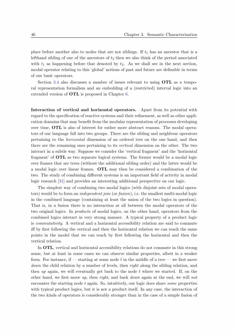
46 Chapter 3. Semantic Characterisation
place before another also to nodes that are not siblings. If t1 has an ancestor that is alefthand sibling of one of the ancestors of t2 then we also think of the period associatedwith t1 as happening before that denoted by t2. As we shall see in the next section,modal operator relating to this ‘global’ notions of past and future are definable in termsof our basic operators.
Section 3.4 also discusses a number of issues relevant to using OTL as a tempo-ral representation formalism and an embedding of a (restricted) interval logic into anextended version of OTL is proposed in Chapter 6.
Interaction of vertical and horizontal operators. Apart from its potential withregard to the specification of reactive systems and their refinement, as well as other appli-cation domains that may benefit from the modular representation of processes developingover time, OTL is also of interest for rather more abstract reasons. The modal opera-tors of our language fall into two groups. There are the sibling and neighbour operatorspertaining to the horizontal dimension of an ordered tree on the one hand, and thenthere are the remaining ones pertaining to its vertical dimension on the other. The twointeract in a subtle way. Suppose we consider the ‘vertical fragment’ and the ‘horizontalfragment’ of OTL as two separate logical systems. The former would be a modal logicover frames that are trees (without the additional sibling order) and the latter would bea modal logic over linear frames. OTL may then be considered a combination of thetwo. The study of combining different systems is an important field of activity in modallogic research [31] and provides an interesting additional perspective on our logic.
The simplest way of combining two modal logics (with disjoint sets of modal opera-tors) would be to form an independent join (or fusion), i.e. the smallest multi-modal logicin the combined language (containing at least the union of the two logics in question).That is, in a fusion there is no interaction at all between the modal operators of thetwo original logics. In products of modal logics, on the other hand, operators from thecombined logics interact in very strong manner. A typical property of a product logicis commutativity. A vertical and a horizontal accessibility relation are said to commuteiff by first following the vertical and then the horizontal relation we can reach the samepoints in the model that we can reach by first following the horizontal and then thevertical relation.
In OTL, vertical and horizontal accessibility relations do not commute in this strongsense, but at least in some cases we can observe similar properties, albeit in a weakerform. For instance, if — starting at some node t in the middle of a tree — we first movedown the child relation by a number of levels, then right along the sibling relation, andthen up again, we will eventually get back to the node t where we started. If, on theother hand, we first move up, then right, and back down again at the end, we will notencounter the starting node t again. So, intuitively, our logic does share some propertieswith typical product logics, but it is not a product itself. In any case, the interaction ofthe two kinds of operators is considerably stronger than in the case of a simple fusion of
3.1 Syntax and Semantics 47
two independent logics.4
While the fusion of two decidable multi-modal logics is known to be itself decidable,products of logics such as the purely vertical and the purely horizontal components ofOTL are notoriously undecidable [31]. This makes OTL an interesting candidate toexamine the question of decidability. In Chapter 5, we are going to give a positiveanswer to this question: OTL is in fact decidable. In the light of our discussion here,this may be considered a surprising result.
A note on the choice of symbols. Our language includes thirteen different symbolsfor the modal operators of OTL (and we are going to introduce even more in the nextsection). Some readers may find this a little confusing at first and may even have theirobjections regarding certain choices (“Why do some transitive operators have a + in thesuperscript while others do not?”). Our reasons for this particular choice of symbolswere as follows. The first objective was to make the language simple. That means firstlyusing familiar symbols (symbols familiar from temporal logics) and secondly avoidingadditions such as sub- or superscripts as far as possible. In the case of the modalities‘pointing’ up, to the left, or to the right in an ordered tree the choice was easy. In allthree cases we have a diamond-operator referring to a node somewhere in the directionindicated by the little bar, a box-operator referring to all nodes in that direction, and anext-operator (i.e. a circle) to refer to the (unique) next node in that direction (if any).So far we have a direct correspondence to the symbols used in standard temporal logics.
The dilemma begins when we have to decide on symbols for the modal operatorspointing down in a tree. Here the concept of a next-operator does not make senseanymore, because typically there will be no unique next node when looking down a tree,but rather several children. Instead, we already need both a universal and an existentialmodality when referring to the immediate successors (i.e. the children) of a node. If westill wish to distinguish transitive and intransitive modalities to speak about descendentsin general and children in particular, then we require two pairs of box- and diamond-operators. In view of our second objective (namely to keep the symbols themselvesas simple as possible and to avoid unnecessary sub- and superscripts) the symbols 3
and 2 should be used for our language, either for the intransitive child operators or forthe transitive descendant operators. Adding a + in the superscript of a given modaloperator is a very simple way of indicating that this new operator is meant to relate tothe transitive closure of the relation underlying the first operator. On the other hand,there is no clear and simple way to do the opposite, that is, to turn a transitive modaloperator into an operator pertaining to the immediate successor relation (not function!)of the former. This is why we have decided to use 3 and 2 to refer to the children of anode and 3+ and 2+ to refer to descendants.
So the fact that, for instance, 3 relates to a transitive relation while 3 does not is
4We are going to provide an axiomatic characterisation of this interaction of vertical and horizontal
operators in Chapter 4 (see remark on page 140).

48 Chapter 3. Semantic Characterisation
in fact not the result of an ‘asymmetric’ choice of symbols, but rather a consequence ofan asymmetric feature of the logic under investigation itself.
3.2 Some Defined Operators
Reflexive transitive closure. Apart from 2 and 3, all box- and diamond-operatorsof OTL correspond to transitive relations. The descendant relation, which correspondsto the modalities 3+ and 2+, is the (non-reflexive) transitive closure of the simple childrelation underlying 3 and 2. As explained earlier, this is indicated by the + in thesuperscript. To indicate a reflexive transitive closure we shall use ∗ rather than +. Thetransitive closure of a transitive relation is just that relation itself. Therefore, we caneasily define modalities which correspond to reflexive transitive closures of some of ouroperators as abbreviations on the syntactic level.
3∗ϕ = ϕ ∨ 3ϕ 2∗ϕ = ϕ ∧ 2ϕ
3∗ϕ = ϕ ∨ 3ϕ 2∗ϕ = ϕ ∧ 2ϕ
3∗ϕ = ϕ ∨ 3ϕ 2∗ϕ = ϕ ∧ 2ϕ
3∗ϕ = ϕ ∨ 3+ϕ 2∗ϕ = ϕ ∧ 2+ϕ
The ancestor relation underlying 2 and 3 is the transitive closure of the parent relationunderlying e. If we required our order over siblings to be (strongly) discrete, then therelation corresponding to 2 and 3 would in fact be the transitive closure of the relationunderlying e (and accordingly for the other direction). In the general case, however, itis possible that a node has a sibling somewhere to the left, but no direct left neighbour.
Universal modality. Observe that, starting anywhere in a tree, the ancestor relationcan take us to the tree’s root, and from there the descendant relation takes us to anynode in the tree. Hence, the two modalities defined next are universal modalities,5 thatis, operators which range over all the nodes in a tree.
3ϕ = 3∗3∗ϕ 2ϕ = 2∗2∗ϕ
Suppose, for example, 2ϕ is true at a certain node t in some model M. Then ϕ mustbe true at every node in M, that is, ϕ must be globally true.
Global past and future modalities. If we further pursue the idea that has led tothe definition of the universal modalities above, we can combine existing modalities insuch a way as to catch not only the siblings to, say, the right of a given node t, but allthe nodes that lie somewhere to the right of t anywhere in the tree. In our extendedtemporal logic setting, such an operator may be described as a ‘global future’ modality.
5A less frequently used but arguably more appropriate term for the universal modality is global
modality. This avoids confusion with the use of the word ‘universal’ to refer to a box-operator (which
has universal meaning) as opposed to a diamond-operator (which has existential meaning).

3.2 Some Defined Operators 49
Global Past•
• • •
• • • •
• • • •
• • • •
3ϕ
ϕ
wwoooooooooooo
444
44
''OOOOOOOOOOOO
///
//
///
//
???
???
zzttttttttt
///
//
$$JJJJJJJJJ
///
//
***
**
***
**
***
**oooo
Global Future•
• •
• • • •
• • •
• • • •
3ϕ
ϕ
wwoooooooooooo
444
44
''OOOOOOOOOOOO
///
//
///
//
???
???
zzttttttttt
///
//
$$JJJJJJJJJ
///
//
***
**
***
**
***
**
LL
LL// //
Figure 3.2: Scope of the global past and future modalities
We think of the nodes representing time points in the future of t as those nodes we canreach by first going up an unspecified number of levels in the tree (or staying at t), thenmaking at least one step to the right (that is, moving to a righthand sibling), and finallymoving down any number of levels (or possibly staying where we are).
Analogously, we can define a global past modality to refer to nodes anywhere to theleft of the current node. Here are the formal definitions of a pair of global past operators3 and 2 and corresponding global future operators 3 and 2:
3ϕ = 3∗33∗ϕ 2ϕ = 2∗22∗ϕ
3ϕ = 3∗33∗ϕ 2ϕ = 2∗22∗ϕ
Figure 3.2 provides a graphical depiction of the scope of our global past and futureoperators. Take, for instance, the tree on the righthand side. The formula 3ϕ is supposedto hold at one of the nodes in the tree. To get to the witness formula ϕ shown in thepicture, we first have to move up two levels in the tree, then move two steps to the right,and finally move down again by one level. The nodes in the scope of 3 are shown aslittle empty circles (), while the rest of the nodes are represented as filled circles (•).The lefthand side of the picture shows a similar example for the case of the existentialglobal past modality.
Difference operator. From the standpoint of a particular given node t in an orderedtree we can partition that tree into four distinct ‘areas’. To start with, there is the branchabove t, which we can refer to using our ancestor modalities 3 and 2, respectively. Thenthere is the subtree below t corresponding to the descendant modalities 3+ and 2+.With the global past and future operators at hand, we can now also refer to the set ofnodes to the left and to the right of t, respectively.
If we combine these four pairs of operators we can define a modality to refer to anynode in the tree but the current one. This kind of modality is known as the differenceoperator in the modal logic literature. Given the following definition, the formula 3ϕ,

50 Chapter 3. Semantic Characterisation
for instance, will be true at a node t iff ϕ is true at some node different from t.
3ϕ = 3ϕ ∨ 3+ϕ ∨ 3ϕ ∨ 3ϕ 2ϕ = 2ϕ ∧ 2+ϕ ∧ 2ϕ ∧ 2ϕ
The difference operator is a very powerful construct6 as it allows us to ‘name’ nodes ina tree. As an example, suppose the formula Q ∧2¬Q is known to be true at node t (insome model). Then Q is true at t but false at every other node in the tree underlyingour model. That is, Q acts as a name (on the syntactic level) for the node t.
Iterated modalities. To express that the same modality is applied n times to a for-mula (with n ∈ N), we can use the following notation.7
2nϕ = 2 · · · 2︸ ︷︷ ︸n times
ϕ
If, for the sake of generality, at some point we are going to use 2nϕ for n ∈ N0, that isfor natural numbers n including 0, then 20ϕ will simply stand for ϕ. The same notationis also used for the other modalities of our language.
Tree features. In our logic, we can easily characterise simple features of nodes in atree, such as being the root or being a leftmost child. For example, a node is the leftmostnode in a group of siblings iff it satisfies the formula 2⊥ (which is equivalent to ¬3>),i.e. iff there are no siblings to its left. The following propositions define roots, leaves,leftmost and rightmost siblings, respectively. The proposition root, for example, is trueat a node t iff t is the root of the tree on which our model is based.
root = 2⊥ leftmost = 2⊥leaf = 2⊥ rightmost = 2⊥
To be precise, the propositions leftmost and rightmost are also satisfied at the rootof a tree.
3.3 Correspondences
In this section, we are going to give a number of examples of simple formulas that canbe used to characterise certain properties of ordered trees (such as being finite or havinga discrete branching factor). The study of these kinds of relationships between syntax(formulas) and semantics (structural properties of frames, or trees in our case) is knownas correspondence theory.
6Blackburn et al. [8], for instance, refer to the difference operator as “the hammer” at the bottom of
their modal logic toolbox.7The set N of natural numbers is the set 1, 2, 3, . . ., that is, 0 is not a natural number.

3.3 Correspondences 51
Bounded branching. In the general case, the orders declared over the children ofa node are not bounded, i.e. there need not be a leftmost or a rightmost sibling. Bypostulating validity of the following proposition we can force the set of children of everynode in a tree to be bounded to either side:
bounded = 3∗leftmost ∧ 3∗rightmost
The formula guarantees the existence of both a leftmost and a rightmost node in every setof children. So bounded is valid in a tree iff that tree is an ordered tree with a boundedbranching factor. Alternatively, we could say that a tree has a bounded branching factorwhenever 2bounded is true at some node in some model based on that tree.
Observe that bounded branching does not necessarily mean that the number of chil-dren of each node has to be finite. A particular node may, for instance, have one childfor every rational number between 0 and 1.
Dense branching. Recall that the children of any given node in a tree form a (strict,but otherwise general) linear order. We may wish this linear order to be dense. Thefollowing formula expresses that the order declared over any set of sibling nodes in thetree underlying a model is required to be dense. No node has either a left or a rightneighbour.8
dense = ¬ e> ∧ ¬ e>Weakly discrete branching. We can also express that every node with a sibling toits left should have a closest left sibling (i.e. a left neighbour) and every node with asibling to its right should have a closest right sibling. We call ordered trees satisfyingthis condition weakly discrete (see Definition A.5 and our discussion of different notionsof discreteness in Appendix A).
weakly-discrete = (3> → e>) ∧ (3> → e>)
Discrete branching. We are now going to characterise trees with a strongly discretebranching factor (that is, between any two sibling nodes there can be only finitely manyother siblings; see also Definition A.6).9 The following proposition is an adaptation ofthe axiom schema (Z) used to characterise (strongly) discrete flows of time for lineartemporal logics [35]. Let A be an arbitrary propositional letter of our language.10 Then
8In fact, it suffices to postulate either ¬ d> or ¬ d> to guarantee that sibling nodes are ordered
densely. If no node can have a lefthand neighbour then no node can have a righthand neighbour either
(and vice versa).9In the sequel, if not further specified, by a discrete order (or branching factor) we mean a strongly
discrete order (branching factor), as opposed to a weakly discrete one.10As will be made precise in Proposition 3.13, discrete is valid in a tree iff that tree has a discrete
branching factor. For formulas, such as bounded, that do not include any propositional letters, this is
equivalent to saying that the formula is globally true in an ordered tree model iff that model is based on

52 Chapter 3. Semantic Characterisation
the following proposition is valid in a tree iff that tree is an ordered tree with a discretebranching factor:
discrete = 2(2A→ A) → (32A→ 2A)
As it may be less evident than our previous examples, we shall formally prove thiscorrespondence result here. First, let us fix a definition of ordered trees with a discretebranching factor.
Definition 3.12 (Discretely ordered trees) An ordered tree T = (T,R, S) is calleda discretely ordered tree iff ([t]R−1R, S) is a strongly discrete order for every node t ∈ T .
Now we can formally state our claim that the formula discrete characterises the classof discretely ordered trees.
Proposition 3.13 (Discrete branching) Let T = (T,R, S) be an ordered tree. ThenT |= discrete holds iff T is a discretely ordered tree.
Proof. To simplify notation we shall write t < t′ for (t, t′) ∈ S and also use t ≤ t′ as anabbreviation for t < t′ or t = t′.
‘⇐’: Suppose < restricted to any set of sibling nodes is a strongly discrete strict linearorder. We need to show that 2(2A→ A) → (32A→ 2A) is true at any given node t inany model M based on T . So let us assume M, t |= 2(2A→ A) (1) and M, t |= 32A
(2). (We need to show M, t |= 2A.)From (1) we get M, t′ |= 2A → A for all t′ with t < t′ (3). From (2) we can infer
that there is a t∗ with t < t∗ and M, t∗ |= 2A (4). Applying modus ponens to (4) and(3) at node t∗ yields M, t∗ |= A (5).
Because < is a strongly discrete order we can define the distance d(t, t∗) of t and t∗
(with t 6= t∗) as the number of elements between t and t∗ plus one. By induction overd(t, t∗), we can now show that M, t |= 2A will be true in any case. For the base case,suppose d(t, t∗) = 1, i.e. t∗ is the direct successor of t. From (4) and (5) we immediatelyobtain M, t |= 2A. For the induction step, we gradually move t forward and keept∗ fixed. So suppose d(t, t∗) = n + 1 (and that the claim has already been shown fordistances up to n). Let t1 be the direct successor of t, i.e. we have d(t1, t∗) = n andhence, by the induction hypothesis, M, t1 |= 2A. Applying modus ponens to the latterand (3) at t1 yields M, t1 |= A. So we get M, t |= 2A, which concludes our proof of thisdirection of the claim.
‘⇒’: Now suppose 2(2A→ A) → (32A→ 2A) is true at every node in every modelbased on T . We need to show that < restricted to any given set of siblings is a stronglydiscrete order. For the sake of contradiction, assume this is not the case, i.e. we have
a tree with the respective property. In the case of discrete, however, if we wish to talk about models
rather than trees, we need to use an instance of discrete for each and every propositional letter in the
language (that is, we need to use it as an axiom schema).

3.3 Correspondences 53
two sibling nodes t1 and t2 with t1 < t2 and there are infinitely many nodes t such thatt1 < t and t < t2. We partially fix a valuation function V as follows:
V (A) = t ∈ T | t < t2 and [t, t2] is finite ∪ t ∈ T | t2 ≤ twhere [t, t2] = t′ ∈ T | t ≤ t′ and t′ ≤ t2
That is, V maps the propositional letter A to the set of those siblings of t1 and t2 thateither lie to the right of t2 or that are only separated from t2 by a finite number of nodes.By definition, the set V (A) will not include t1.
Now consider the model M = (T , V ) and check whether M, t1 |= discete holds(as it should). We have M, t |= A for all t ∈ V (A) and M, t 6|= 2A for all t ∈ T witht < t2 and t 6∈ V (A). Hence, the implication 2A → A will be true at any sibling oft2. In particular, we get M, t1 |= 2(2A → A). Because of M, t2 |= 2A we also getM, t1 |= 32A. On the other hand, we have M, t1 6|= 2A, i.e. we get M, t1 6|= discrete.This is a contradiction to the premise that discrete is valid in T , i.e. our assumptionthat < restricted to any set of siblings is not discrete must be false. 2
Finite branching. For many applications, trees with a finite (or even a fixed) branch-ing factor will be sufficient. We can restrict models to those based on finitely branchingtrees by forcing the branching factor to be both bounded and strongly discrete.
finite-branching = bounded ∧ discrete
We can also fix a specific finite branching factor. Let n ∈ N. Then the following formulacharacterises a tree with branching factor n:
branching(n) = ¬leaf → 3(leftmost ∧ en−1rightmost)
This formula is true at an internal node (i.e. a node that is not a leaf) iff it has got achild that is a leftmost sibling which in turn has got a rightmost sibling n − 1 steps toits right. Hence, every node that has any children at all will have exactly n children.The formula branching(2), for instance, is valid in an ordered tree iff that tree is abinary tree. An alternative way of characterising the class of binary trees is given by thefollowing formula:
binary = (leftmost ↔ rightmost) → root
For any node that is not the root of a tree, the above formula can only be true ifleftmost and rightmost have distinct truth values. Hence, every node but the roothas to be either a leftmost or a rightmost sibling, but not both.
Blackburn and Meyer-Viol [9] have developed a modal logic of finite binary trees. Asdemonstrated by the authors, such trees have important applications in computationallinguistics. For binary trees, we can easily define modalities to refer to the left or rightchild of a given node. The formula 3(leftmost ∧ ϕ), for example, is true at a node twhenever t has got a left child at which ϕ is true.

54 Chapter 3. Semantic Characterisation
Finite depth. The following is an adaptation of Blackburn and Meyer-Viol’s axiom(F3). It characterises trees of finite depth. Again, A may be any propositional letter.
finite-depth = A → 3∗(A ∧2+¬A)
We can easily check that finite-depth is valid in trees of finite depth. Whenever aformula A is true at some node t then on any of the (finite) branches below t there mustbe a last occurrence of A (this could be at t itself). At that node of last occurrence(which may be a leaf node) the formula A ∧2+¬A is true.
For the other direction, i.e. to show that finite-depth being valid in a tree forcesthat tree to be of finite depth, we shall only sketch a proof here. Let T be a tree with aleast one infinite branch (we will show that it does not validate finite-depth). We fixa valuation V for the propositional letter A as follows. Let A be false in the leaves of Tas well as any internal nodes that dominate solely finite branches. For all other nodes twe declare an alternating valuation: let A be true at t iff the depth of t in the tree (thatis, the distance from the root) is an even number. This means, in particular, that A istrue at the root of T (because there must be at least one infinite branch). Then, in themodel M = (T , V ), the formula finite-depth does not hold at the root of T : A is trueat the root, but there is no node t in the tree such that A is true at t and false at everynode below t.
Characterising trees that have only infinite branches, that is, trees without leaves isconsiderably easier than axiomatising finite depth. A model is based on an ordered treewithout leaves iff the formula ¬leaf is globally true in that model. Observe that ¬leaf
is equivalent to 3>, the seriality axiom with respect to the existential child modality.
Degenerate trees. In general, a node may have any number of children. However,for certain purposes we may regard a tree where some nodes have a single child as adegenerate tree. For instance, if we use OTL as an extended temporal logic we may runinto problems when we interpret the single child t1 of a node t2 as a time period duringthe period associated with t2. Such an interpretation would entail that period t1 shouldbe strictly shorter than t2. On the other hand, one may wish to interpret t1 and t2 asthe same time periods. In order to avoid problems of this kind in the first place, we maywish to restrict our attention to the class of non-degenerate trees, that is, to trees whereevery internal node has got at least two children.
The following formula is valid in a tree iff every node in that tree besides the root isnot both the leftmost and the rightmost member of a set of siblings. This excludes thepossibility of single children.
non-degenerate = (leftmost ∧ rightmost) → root

3.4 Ontological Considerations 55
3.4 Ontological Considerations
We may wish to use the logic of ordered trees to model the behaviour of a complexsystem changing over time. Here, time runs from left to right (that is, along the relationunderlying 3), and the children of a node allow us to zoom into a particular period oftime to specify the system in more detail. If we start thinking about OTL as a temporalrepresentation language, we will soon encounter a number of questions and possiblyeven, initially, entertain doubts regarding the logic’s adequacy for such an undertaking.Suppose we have ϕ being true at some node t. If we think of the children of t as a morefine-grained representation of the time period associated with t, then should this notimply that ϕ must also hold at any of the children of t?
The best possible answer to such a question would be: it depends. In fact, it dependson the ontology of ϕ. What kind of proposition is ϕ supposed to represent?
Ontological categories. Suppose, for example, that ϕ stands for ‘Mary travelled allthe way from Islington to Aldwych’. In that case, ϕ may very well be true at somenode t, but false at one of t’s children (that is, during a time period within the onecorresponding to t). In fact, we might even want to enforce ¬ϕ for all descendants oft as Mary cannot complete her entire journey both over the duration of t and also in ashorter period within t.11 If, on the other hand, ϕ stands for a proposition like ‘Maryhas long blonde hair’ then we do want ϕ to hold at descendants of t as well. In theliterature on foundations of planning in artificial intelligence propositions of the latterkind have been called properties or facts, while propositions like ‘Mary travelled all theway from Islington to Aldwych’ are known as events [2, 54, 65].12
Such ontological distinctions often form an integral part of the definition of a planningformalism. In Allen’s work [2], for example, the definition of the predicates holds andoccur, which are used to distinguish between different types of propositions, is central tothe entire system. holds is applied only to properties and occur is reserved for the usewith occurrences (an ontological category that includes events). While Allen’s approachhas undoubtedly been one of the most influential in this area, it has also received acertain amount of criticism. Shoham [65], in particular, argues against the “seductiveunclarity” of a logic with this kind of built-in ontology. He proposes that, in the firstinstance, one should rather not make any specific commitments to ontology, but thenallow for the definition of a fine ontological structure on top of the basic formalism.
This is also the approach we have taken in the definition of our logic. Propositionsin OTL are just that: propositions. Initially, we do not associate them with any spe-cific ontological category (such as properties or events). However, certain ontological
11We should stress that we are not concerned with the grammatical tense of the verb ‘travelled’ here.
The proposition ‘Mary travelled all the way from Islington to Aldwych’ being true at node t is interpreted
as Mary completing her journey during the time period t, not during some period in the past of t.12In the area of software engineering, the corresponding ontological categories are sometimes referred
to as states and actions, respectively [23, 46].

56 Chapter 3. Semantic Characterisation
categories can be defined within the logic. In this section we give a number of examples.
Homogeneity. According to the semantics given for OTL, a formula ϕ being satisfiedat some node t does not imply that ϕ also has to hold at all nodes that are below t in thetree. Whether this is appropriate or not depends on the kind of proposition representedby the formula ϕ.
Propositions like ‘Mary has long blonde hair’, i.e. properties, are homogeneous: ‘tem-porally’ speaking, a homogeneous proposition ϕ is true iff it is true at every time intervalwithin the reference interval. Following Shoham [65] we define homogeneous propositionsas propositions that are both downward-hereditary and upward-hereditary. A proposi-tion is called downward-hereditary if whenever it holds at some node it also holds atall descendants of that node. Analogously, a proposition is called upward-hereditary ifwhenever it holds at all descendants of a given node it also holds at that node itself(assuming that node has any descendants at all).
down-hered(ϕ) = ϕ → 2+ϕ
up-hered(ϕ) = 3> → (2+ϕ → ϕ)hom(ϕ) = down-hered(ϕ) ∧ up-hered(ϕ)
So ϕ is a homogeneous proposition (with respect to a given model) iff hom(ϕ) is globallytrue in that model.
Strong negation. Negation as we have defined it here is weak in the sense that ¬ϕbeing satisfied at a particular node simply means that it is not the case that ϕ is satisfiedat that node. It does, however, not preclude ϕ from being satisfied at some of thedescendants of that node. For propositions corresponding to certain kinds of ontologicalcategories the notion of strong negation may be more appropriate. We can define a strongnegation operator as follows:
∼ϕ = 2∗¬ϕ
The formula ∼ϕ is true at a node t iff ϕ is false at t and all nodes that are descendantsof t. What kind of properties does this new operator have? The following proposition,for instance, gives us a restricted version of de Morgan-like laws for strong negation. Wemay rewrite ∼ϕ∧ ∼ψ as ∼ (ϕ ∨ ψ) and vice versa. We may also rewrite ∼ϕ∨ ∼ψ as∼(ϕ ∧ ψ), but not the other way round.
Proposition 3.14 (Restricted de Morgan laws for strong negation) The fol-lowing hold for all formulas ϕ and ψ:
(1) |= ∼ϕ∧ ∼ψ ↔ ∼(ϕ ∨ ψ)
(2) |= ∼ϕ∨ ∼ψ → ∼(ϕ ∧ ψ)

3.4 Ontological Considerations 57
Proof. (1) We show that the formulas ∼ϕ∧ ∼ψ and ∼ (ϕ ∨ ψ) are equivalent: ∼ϕ∧ ∼ψ ≡ 2∗¬ϕ ∧2∗¬ψ ≡ 2∗(¬ϕ ∧ ¬ψ) ≡ 2∗¬(ϕ ∨ ψ) ≡ ∼(ϕ ∨ ψ).
(2) Suppose ∼ ϕ∨ ∼ ψ, which is equivalent to 2∗¬ϕ ∨ 2∗¬ψ, is true. Then also2∗(¬ϕ ∨ ¬ψ) has to be true. The latter is equivalent to 2∗¬(ϕ ∧ ψ), which in turn isequivalent to ∼(ϕ ∧ ψ). 2
To see that indeed ∼ ϕ∨ ∼ ψ and ∼ (ϕ ∧ ψ) are not equivalent, i.e. that the oppositedirection of (2) would not be valid, consider the following counterexample. Suppose wehave a tree consisting only of a root node with a single child. Further suppose that ϕholds at the root, but not the child, and that ψ holds at the child node, but not at theroot. Then ∼ (ϕ ∧ ψ) is clearly true at the root, because at no node both ϕ and ψ aretrue. However, ∼ϕ∨ ∼ψ does not hold at the root, because for neither ϕ nor for ψ it isthe case that they do not hold at any of the two nodes.
The following result suggests that ∼ may be the appropriate negation operator to beapplied to homogeneous propositions.
Proposition 3.15 (Strong negation of homogeneous propositions) The strongnegation of a homogeneous proposition ϕ is itself homogeneous, that is, global truth ofhom(ϕ) implies global truth of hom(∼ϕ).
Proof. We start by showing that the strong negation of any proposition (that is, notjust that of homogeneous ones) is downward-hereditary. It is easy to see that 2∗¬ϕ →2+2∗¬ϕ is a valid formula. This is equivalent to down-hered(∼ϕ), which means thatthe strong negation of any formula ϕ will be downward-hereditary.
Next we prove that ∼ϕ is upward-hereditary under the assumption that ϕ is homo-geneous. We need to show the global truth of up-hered(∼ϕ), i.e. that given 3> and2+2∗¬ϕ at some node t we can infer that 2∗¬ϕ is also true at t. Observe that 2+2∗¬ϕis equivalent to 2+¬ϕ, so we only need to show that we can infer ¬ϕ. For the sake ofcontradiction, suppose that ϕ is true at t. Because t has descendants (enforced by 3>)and because ϕ is homogeneous, t will have descendants satisfying ϕ. This contradicts2+¬ϕ. Hence, both ¬ϕ and 2+¬ϕ, and therefore also 2∗¬ϕ, need to be true at t. Thiscompletes our proof of Proposition 3.15. 2
Strong double negation. We have ∼∼ϕ ≡ 2∗¬2∗¬ϕ ≡ 2∗3∗ϕ. As 2∗ϕ implies2∗3∗ϕ it is easy to see that the formula ϕ →∼∼ ϕ must be true for homogeneouspropositions ϕ.
The converse, however, does not hold, that is, we cannot eliminate a strong doublenegation, not even for homogeneous propositions. To see this, consider the followingcounterexample. Let T be an infinite binary tree where every right child is a leaf (i.e.there is one long branch to the left with many short ones to the right). Let ϕ be theonly propositional letter in our language and define the ordered tree model M = (T , V ),with V (ϕ) being the set of all right children. Then 2∗3∗ϕ (and thereby ∼∼ϕ) is truein the root of T , but ϕ is not.

58 Chapter 3. Semantic Characterisation
Finally, it is worth noting that over trees of finite depth the formula ∼∼ϕ→ ϕ actu-ally is globally true for homogeneous propositions ϕ.13 This can be shown by inductionover the height of a node in a tree. For the base case, assume we are in a leaf node. Then∼∼ϕ, which is equivalent to 2∗3∗ϕ, directly implies ϕ. For the induction step, assumewe are in a node t of height n + 1, that is, all branches below t have at most length n.Let ∼∼ϕ be true at t. By Proposition 3.15, ∼∼ϕ is homogeneous, i.e. ∼∼ϕ also holdsin every node below t. Now, by the induction hypothesis, we can conclude that ϕ mustbe true at every node below t. As ϕ is homogeneous, this means that ϕ must also holdat t itself.
Comparison with Allen’s system. It is interesting to compare our discussion of ho-mogeneity and strong negation with Allen’s holds predicate used to characterise prop-erties in [2]. Allen’s definition of strong negation is essentially the same as ours andhis properties roughly correspond to our homogeneous propositions. What is differentis that the strong negation operator of [2] is involutive, that is, elimination of strongdouble negation is a valid operation for those ‘homogeneous’ propositions. In fact, Allencharacterises his properties as precisely those propositions ϕ that validate ϕ↔ 2+3+ϕ
(translated into our formalism). That is, a proposition ϕ is called a property (a ‘homo-geneous’ proposition) iff ϕ being true at t is equivalent to ϕ being true infinitely manytimes on every branch below t. In Allen’s setting, where every interval has subinter-vals (every node has children, in our formalism), this is a stronger requirement14 thanjust postulating the equivalence of ϕ and 2+ϕ (see [2] for a proof). As Allen definesthe strong negation of a property ϕ as 2+¬ϕ (i.e. ∼∼ ϕ is equivalent to 2+3+ϕ), weimmediately get ∼∼ϕ ≡ ϕ.
Strict implication. Our implication operator → has classical semantics: ϕ → ψ istrue at a node t whenever ϕ is false at t or ψ is true at t. We may also wish to employthe concept of strict implication: a proposition ϕ strictly implies another proposition ψ(at a node t) iff whenever ϕ is true at a descendent t′ of t (including t itself) then alsoψ is true at t′. Such a strict implication operator ⇒ can be defined as follows:
ϕ⇒ ψ = 2∗(ϕ→ ψ)
The connection between strong negation and strict implication is summarised in theequivalence ∼ ϕ ≡ ϕ⇒ ⊥, the validity of which is readily verified.
Connections to intuitionistic logic. In the proof of Proposition 3.15 it has beennoted that ∼ ϕ is a downward-hereditary formula for any formula ϕ. By the sameargument, we can show that also ϕ ⇒ ψ (strict implication) is downward-hereditaryfor any ϕ and ψ. Furthermore, it is easily observed that both ϕ ∧ ψ and ϕ ∨ ψ are
13This observation is due to Naza Aguirre (personal communication).14See also Shoham’s critique of Allen’s definition of the holds predicate in [65].
3.4 Ontological Considerations 59
downward-hereditary whenever ϕ and ψ are. In other words, the set of downward-hereditary propositions is closed under application of ∼, ∧, ∨, and ⇒.
At this point it is interesting to observe that, for downward-hereditary propositions,the ∼,∧,∨,⇒-fragment of our logic coincides with propositional intuitionistic logic.This can be seen by comparison with the definition of the possible worlds semantics forintuitionistic logic as given, for instance, in [72].15 In particular, observe that the law ofthe excluded middle does not hold for the strong negation operator ∼. Formulas of theform ∼ ϕ ∨ ϕ are not necessarily globally true in all models, even when ϕ is downward-hereditary. A simple counterexample would be any model where ¬ϕ holds at one nodebut ϕ is true at one of its children.
Other ontological categories. The notion of homogeneity has been discussed in somedetail here as it is probably the most important ontological concept in the context oftemporal reasoning. We are going to give two more examples of ontological categories.
The first one concerns the characterisation of events. An event, that is, a propositionlike our ‘Mary travelled all the way from Islington to Aldwych’ should not hold over twotime periods one of which properly contains the other. Shoham [65] calls propositions ofthis type gestalt.16 In the context of a tree, we can interpret this condition as follows.A proposition ϕ is gestalt iff whenever ϕ is true at a node t then it must be false at allancestors and descendants of t.
gestalt(ϕ) = ϕ → (2¬ϕ ∧ 2+¬ϕ)
Another ontological concept that can be expressed is locality. A proposition ϕ is calledlocal if ϕ is true during a particular time period iff it is true at the beginning of thatperiod [37]. In our system, the beginning of a time period may be identified with theleftmost child of a node. The following definition takes into account that a node doesnot necessarily have to have a leftmost child (although we may wish to postulate thatproperty independently, as outlined in the previous section).
local(ϕ) = (3leftmost ∧ ϕ) ↔ 3(leftmost ∧ ϕ)
What we have seen here are just examples. Hopefully, they give some impression ofthe variety of options available to us when using OTL as a temporal representationformalism.
15The semantics of intuitionistic logic can be defined via possible world models with frames that are
partial orders and persistent valuation functions (that is, a propositional letter that is true at some world
cannot be false at a later world). The aspect of persistence is captured by our restriction to downward-
hereditary propositions. Also observe that the accessibility relation R∗ underlying the modality 2∗ is a
partial order. The fact that R∗ is generated by a tree is not a restriction, because in the definition of the
semantics of intuitionistic logic the accessibility relation is only used ‘in one direction’.16Related to this, Shoham also defines the class of solid propositions, that is, propositions that cannot
be true at overlapping time intervals. This would provide an alternative way to characterise events, but
the notion of overlapping intervals cannot be represented in OTL.

60 Chapter 3. Semantic Characterisation
3.5 General Models and P-morphisms
In this and the following section we are going to take a closer look at the semanticsof OTL. At the beginning of this chapter we have defined our logic as a modal logicover frames that are ordered trees and we have given the various modal operators of ourlanguage a semantics by referring to intuitive notions such as ‘left sibling’ or ‘parent’.Taking a somewhat broader view, we could also think of OTL as a multi-modal logicover frames with two basic accessibility relations R (the child relation) and S (the orderdeclared over siblings). The meaning of our modal operators can then be defined in termsof these basic relations and a number of compound accessibility relations constructedfrom R and S.
In our intended semantics, the relation R is required to characterise a tree and S
is required to be a linear order for each and every set of sibling nodes in that tree.Loosening these constraints on R and S slightly may not always change the logic, in thesense that the same formulas as before may be those that have models. In what follows,we are going to make precise this idea of widening the class of admissible frames.17 Ourmain technical tool will be certain types of mappings between frames that are known asp-morphisms.
General models. Our first aim will be to give an alternative definition of the semanticsof our logic, namely as a multi-modal logic with a number of compound accessibilityrelations based on the basic relations R and S. To this end, we are going to introducethe notion of a general model where we drop the constraints on the basic accessibilityrelations R and S completely. This will provide us with a basis upon which we arelater going to define manipulations of the accessibility relations that are satisfiabilitypreserving.
Next-operators with general models? Our modal language includes a number ofnext-operators. Defining the semantics of formulas with next-operators over generalmodels is problematic, because it is not clear how to generalise the notion of a next statewhen moving from orders with unique immediate successors to general relations.
Rather than attempting to generalise this notion, we will simply think of next-operators as ordinary diamond-operators, that is, we do not generally require the under-lying accessibility relation to be functional. For example, in our intended models (modelsbased on ordered trees) the parent relation R−1 is functional, that is, any node can haveat most one parent. For the general models, we will drop this condition and treat the
17At this point it maybe worthwhile to point out that the material of this and the following section is
not only intended to provide us with a deeper understanding of the model-theoretic semantics of OTL,
but will also be required to prove completeness for the axiomatisation discussed in Chapter 4. In fact,
the aforementioned ‘wider class of admissible frames’ (which we are going to give a precise definition for
later on, cf. loosely ordered trees) is precisely the class of frames we encountered during our initial efforts
to prove completeness for a preliminary set of axioms.

3.5 General Models and P-morphisms 61
parent modality e as an existential modality (i.e. like a diamond-operator) over R−1.In our intended models the accessibility relation underlying e (the right sibling re-
lation) is definable in terms of S, namely as S \ S S. This definition makes sense,because we know that S is not branching to the right. Hence, it captures the notion ofan immediate successor. In the general setting, where S could be any binary relation,such a definition would seem rather arbitrary and we shall not adopt it. Instead, we willintroduce a third accessibility relation N , which only in intended models will be requiredto coincide with the immediate successor relation induced by S.
Definition 3.16 (General frames) A general frame is a quadruple F = (T,R, S,N)where T is a non-empty set, and R, S and N are binary relations over T . The elementsof T are called worlds.
As for the case of ordered trees before, we shall occasionally simply refer to worlds t ina frame F rather than explicitly introducing a set of worlds T for that frame first.
When speaking about an intended frame we shall mean a frame that corresponds toan ordered tree. In other words, a general frame F = (T,R, S,N) is called an intendedframe if (T,R, S) is an ordered tree and N = S \ S S, that is, for every node in thetree N points to its immediate righthand successor with respect to the linear order S,whenever there is such a successor.
Definition 3.17 (General models) A general model is a pair M = (F , V ) where F =(T,R, S,N) is a general frame and V is a valuation, that is, a mapping from propositionalletters to subsets of the set of worlds T .
Again, we may either write M = (F , V ) with F = (T,R, S,N) or directly M =(T,R, S,N, V ). In Definition 3.18 we are going to fix the notion of truth for generalmodels. The semantics of our various modalities will be defined with respect to (possiblycomplex) accessibility relations depending on R, S and N . The relation S−1, for exam-ple, will be used to refer to those worlds that, within an ordered tree model, we wouldcall left siblings.
The following definition should be read in conjunction with Definition 3.6, where thenotion of truth for our intended models has been defined.
Definition 3.18 (Truth in a general model) We inductively define the notion of aformula being true in a general model M = (F , V ) with F = (T,R, S,N) at a worldt ∈ T as follows:
(1) M, t |= P iff t ∈ V (P ) for propositional letters P ;
(2) M, t |= >;
(3) M, t |= ¬ϕ iff M, t 6|= ϕ;
(4) M, t |= ϕ ∧ ψ iff M, t |= ϕ and M, t |= ψ;

62 Chapter 3. Semantic Characterisation
(5) M, t |= eϕ iff there is a t′ ∈ T with (t, t′) ∈ R−1 and M, t′ |= ϕ;
(6) M, t |= 3ϕ iff there is a t′ ∈ T with (t, t′) ∈ (R−1)+ and M, t′ |= ϕ;
(7) M, t |= eϕ iff there is a t′ ∈ T with (t, t′) ∈ N−1 and M, t′ |= ϕ;
(8) M, t |= 3ϕ iff there is a t′ ∈ T with (t, t′) ∈ S−1 and M, t′ |= ϕ;
(9) M, t |= eϕ iff there is a t′ ∈ T with (t, t′) ∈ N and M, t′ |= ϕ;
(10) M, t |= 3ϕ iff there is a t′ ∈ T with (t, t′) ∈ S and M, t′ |= ϕ;
(11) M, t |= 3ϕ iff there is a t′ ∈ T with (t, t′) ∈ R and M, t′ |= ϕ;
(12) M, t |= 3+ϕ iff there is a t′ ∈ T with (t, t′) ∈ R+ and M, t′ |= ϕ.
Observe that in case the underlying frame F = (T,R, S,N) is such that (T,R, S) isan ordered tree and N = S \ S S, the above notion of truth coincides with the oneoriginally formulated in Definition 3.6. The remaining operators of our language canagain be considered defined operators; see Definition 3.7.
While we are going to reserve the term ‘satisfiable’ for formulas that have an orderedtree model, we are going to speak about formulas that are satisfiable in a general modelbased on some frame belonging to a certain class of frames.
Definition 3.19 (Satisfiability in general models) We say a formula ϕ is satisfi-able in a model based on a frame belonging to some class of general frames iff there is ageneral model M = (F , V ) based on a frame F from that class with a world t in F suchthat M, t |= ϕ holds.
The concepts of global truth, validity with respect to a particular frame, and validity ingeneral can be defined in analogy to Definitions 3.9, 3.10 and 3.11, respectively.
P-morphisms. The notion of p-morphism (or bounded morphism) plays a centralrole in the study of modal logics [8, 13, 35]. It provides us with a powerful tool todescribe satisfiability preserving transformations between models. Further below we willstate the definition of p-morphisms for our particular modal logic with three accessibilityrelations, all of which are used ‘in both directions’. We start by introducing the conceptof p-morphism for pairs of a domain and a binary relation declared over that domain.
Definition 3.20 (P-morphisms for relational structures) Let T and T ′ be setsand let R be a binary relation over T and R′ a binary relation over T ′. A functionf : T → T ′ is called a (simple) p-morphism from (T,R) to (T ′, R′) iff it satisfies thefollowing conditions:
(1) if (t1, t2) ∈ R then (f(t1), f(t2)) ∈ R′;
(2) if (f(t1), t′2) ∈ R′ then there is a t2 ∈ T with f(t2) = t′2 and (t1, t2) ∈ R.

3.5 General Models and P-morphisms 63
We call f a bidirectional p-morphism, if in addition to the above it also satisfies thefollowing condition:
(3) if (t′1, f(t2)) ∈ R′ then there is a t1 ∈ T with f(t1) = t′1 and (t1, t2) ∈ R.
The first of these conditions is sometimes called the homomorphic condition as it guaran-tees f to be a homomorphism. The second condition has been called the back conditionin [8] and the third one may be called the inverse back condition. If in the above def-inition the p-morphism f is a surjective function then (T ′, R′) is called the p-morphicimage of (T,R).
Next we are going to introduce the notion of p-morphism for our general frames. Inshort, we call a function a p-morphism from one frame to another if that function isa bidirectional p-morphism with respect to the three accessibility relations of a generalframe.
Definition 3.21 (P-morphisms for frames) Let F = (T,R, S,N) and F ′ =(T ′, R′, S′, N ′) be general frames. A function f : T → T ′ is called a p-morphism from Fto F ′ iff it satisfies the following conditions:
(1) f is a bidirectional p-morphism from (T,R) to (T ′, R′);
(2) f is a bidirectional p-morphism from (T, S) to (T ′, S′);
(3) f is a bidirectional p-morphism from (T,N) to (T ′, N ′).
We are not going to distinguish simple and bidirectional p-morphisms for frames. Whenspeaking about a p-morphism in the context of a general frame we shall always mean abidirectional p-morphism. Again, if the p-morphism f is a surjective function from T
onto T ′, then the frame F ′ is called the p-morphic image of F .Finally, we extend the notion of p-morphisms to general models.
Definition 3.22 (P-morphisms for models) Let M = (F , V ) and M′ = (F ′, V ′) begeneral models with F = (T,R, S,N) and F ′ = (T ′, R′, S′, N ′). A function f : T → T ′
is called a p-morphism from M to M′ iff it satisfies the following conditions:
(1) f is a p-morphism from (F , R) to (F ′, R′);
(2) t ∈ V (P ) iff f(t) ∈ V ′(P ) for all t ∈ T and all propositional letters P .
Also in the case of models, if there exists a p-morphism f from M to M′ that is asurjective function then we say that M′ is a p-morphic image of M.
As will be stated as Theorem 3.24 below, the truth of a formula ϕ in a general modelM is invariant under p-morphisms. The proof of that theorem will make use of thefollowing lemma.

64 Chapter 3. Semantic Characterisation
Lemma 3.23 (P-morphisms for compound relations) Let f be a bidirectional p-morphism from (T,R1) to (T ′, R′
1) and from (T,R2) to (T ′, R′2). Then also the following
are true:
(1) f is a bidirectional p-morphism from (T,R−11 ) to (T ′, R′−1
1 );
(2) f is a bidirectional p-morphism from (T,R1 ∪R2) to (T ′, R′1 ∪R′
2);
(3) f is a bidirectional p-morphism from (T,R1 R2) to (T ′, R′1 R′
2);
(4) f is a bidirectional p-morphism from (T,Rn1 ) to (T ′, R′n
1 ) for all n ∈ N;
(5) f is a bidirectional p-morphism from (T,R+1 ) to (T ′, R′+
1 );
(6) f is a bidirectional p-morphism from (T,R∗1) to (T ′, R′∗
1 ).
Proof. For each of the six statements we have to show that the three conditions for p-morphisms formulated in Definition 3.20 also hold for the complex relation in question.
(1) Inverse. (1) If (t1, t2) ∈ R−11 then (t2, t1) ∈ R1, which implies (f(t2), f(t1)) ∈
R′1 (because f is a p-morphism with respect to R1), which in turn implies
(f(t1), f(t2)) ∈ R′−11 .
(2) If (f(t1), t′2) ∈ R′−11 then (t′2, f(t1)) ∈ R′
1, i.e. there exists a t2 ∈ T such thatf(t2) = t′2 and (t2, t1) ∈ R1, which implies (t1, t2) ∈ R−1
1 .
Condition (3) is dual to condition (2) and can be checked analogously.
(2) Union. (1) (t1, t2) ∈ R1 ∪ R2 implies either (t1, t2) ∈ R1 or (t1, t2) ∈ R2. Thatis, we get (f(t1), f(t2)) ∈ R1 or (f(t1), f(t2)) ∈ R2, hence the desired result(f(t1), f(t2)) ∈ R1 ∪R2.
(2) Let (f(t1), t′2) ∈ R′1 ∪R′
2, i.e. either (f(t1), t′2) ∈ R′1 or (f(t1), t′2) ∈ R′
2. Hence,there must be a t2 ∈ T with f(t2) = t′2 satisfying either (t1, t2) ∈ R1 or (t1, t2) ∈ R2,and thereby also (t1, t2) ∈ R1 ∪R2.
Condition (3) is checked analogously.
(3) Composition. (1) Let (t1, t3) ∈ R1 R2, i.e. there is a t2 ∈ T such that (t1, t2) ∈ R1
and (t2, t3) ∈ R2 hold. Because f is a p-morphism for both R1 and R2 we get(f(t1), f(t2)) ∈ R′
1 and (f(t2), f(t3)) ∈ R′2, hence (f(t1), f(t3)) ∈ R′
1 R′2.
(2) Let (f(t1), t′3) ∈ R′1 R′
2 i.e. there is a t′2 ∈ T ′ such that (f(t1), t′2) ∈ R′1
and (t′2, t′3) ∈ R′
2 hold. Because f is a p-morphism for R1, there is a t2 ∈ T
with f(t2) = t′2 and (t1, t2) ∈ R1. As we also obtain (f(t2), t′3) ∈ R′2 and f is
a p-morphism with respect to R2, there has to be a t3 ∈ T with f(t3) = t′3 and(t2, t3) ∈ R2. Finally, we therefore get (t1, t3) ∈ R1 R2.
Condition (3) is checked analogously.

3.5 General Models and P-morphisms 65
(4) Iteration. Given the result for the composition of relations, it can easily be shownby complete induction that f is a bidirectional p-morphism from (T,Rn
1 ) to (T,R′n1 )
for any n ∈ N.
(5) Transitive closure. Checking the three p-morphism conditions for the transitiveclosure is now straightforward:
(1) Let (t1, t2) ∈ R+1 , that is, there exists an n ∈ N such that (t1, t2) ∈ Rn
1 . Butthen also (f(t1), f(t2)) ∈ R′n
1 for the same n, i.e. (f(t1), f(t2)) ∈ R′+1 .
(2) Let (f(t1), t′2) ∈ R′+1 , i.e. (f(t1), t′2) ∈ R′n
1 for some n ∈ N. So there exists at2 ∈ T with f(t2) = t′2 and (t1, t2) ∈ Rn
1 , hence also (t1, t2) ∈ R+1 .
Condition (3) is checked analogously.
(6) Reflexive transitive closure. First observe that any function from T to T ′ mustbe a bidirectional p-morphism from (T,=) to (T ′,=). Given that the reflexivetransitive closure of a relation is the union of the non-reflexive transitive closure ofthat relation and =, the desired result follows immediately from cases (2) and (5).
This concludes our proof of Lemma 3.23. 2
We should point out that p-morphisms are not generally preserved under taking com-plements or forming either intersections or differences of relations.18
The following P-morphism Theorem is, essentially, a standard result in modal logics.What is a little different in our case is that the results proved in Lemma 3.23 allowus to limit the checking of the p-morphism conditions to the three basic accessibilityrelations of a model (namely R, S and N) rather than checking them for all of theeight compound accessibility relations referred to in the definition of the semantics ofour modal operators.19
Theorem 3.24 (P-morphisms) Let M = (F , V ) and M′ = (F ′, V ′) be general modelswith F = (T,R, S,N) and F ′ = (T ′, R′, S′, N ′), and let f be a (bidirectional) p-morphismfrom M to M′. Then for all worlds t ∈ T and all formulas ϕ we have:
M, t |= ϕ iff M′, f(t) |= ϕ
Proof. By induction on the structure of formulas ϕ. For the base case, assume ϕ is apropositional letter. The statement then is a direct consequence of the second conditionfor p-morphisms formulated in Definition 3.22. It is also trivially true for the formula >.
18Here is a simple counterexample for the case of the difference operation. Let T = t1, t2 and
T ′ = t′ and define the following relations over these two domains: R1 = (t1, t1), (t1, t2), (t2, t2), R2 =
(t1, t1), (t2, t2), R′1 = (t′, t′), and R′
2 = (t′, t′). Then the function f with f(t1) = t′ and f(t2) = t′ is
a bidirectional p-morphism both from (T,R1) to (T ′, R′1) and from (T,R2) to (T ′, R′
2), because all three
conditions of Definition 3.20 are fulfilled. However, f is not a p-morphism from (T,R1\R2) to (T ′, R′1\R′
2),
because the homomorphic condition fails for one pair of elements: although we have (t1, t2) ∈ R1\R2,
the required (f(t1), f(t2)) ∈ R′1\R′
2 does not hold.19See items (5)–(12) in Definition 3.18.

66 Chapter 3. Semantic Characterisation
For the induction step, we have to consider all the core operators of our language.Those are the operators referred to in Definition 3.18. The definable operators fromDefinition 3.7 need not be considered here. We start with the propositional connectives:
(1) Negation. We have M, t |= ¬ϕ iff M, t 6|= ϕ, which by the induction hypothesis isequivalent to M′, f(t) 6|= ϕ, which in turn is equivalent to M′, f(t) |= ¬ϕ.
(2) Conjunction. We have M, t |= ϕ ∧ ψ iff both M, t |= ϕ and M, t |= ψ. By theinduction hypothesis this is equivalent to M′, f(t) |= ϕ and M′, f(t) |= ψ, i.e.M′, f(t) |= ϕ ∧ ψ.
Next we turn to the modal operators. The formulations of the truth conditions forthe various modal operators in Definition 3.18 have a common structure: truth of aformula requires the existence of a successor world with respect to a (possibly complex)accessibility relation and the truth of the main subformula of the formula in question atthat world. These accessibility relations are all constructed from R, S, and N using onlythe operations of inverse and transitive closure, both of which are covered by Lemma 3.23.That is, f is a p-morphism with respect to all these relations (and the correspondingrelations of M′).
These observations allow us to treat all modal operators in the same way. For theinduction step for the case of a modal operator applied to a principal subformula ϕ, weshall prove the following general claim:
Claim: If α and α′ are binary relations such that f is a p-morphism from(T, α) to (T ′, α′) then, for all t ∈ T and all formulas ϕ (covered by theinduction hypothesis), there exists a tα ∈ T with (t, tα) ∈ α and M, tα |= ϕ
iff there exists a t′α ∈ T ′ with (f(t), t′α) ∈ α′ and M′, t′α |= ϕ.
‘⇒’: Assume there exists a tα ∈ T with (t, tα) ∈ α and M, tα |= ϕ. From the in-duction hypothesis we get M′, f(tα) |= ϕ and from the homomorphic condition we get(f(t), f(tα)) ∈ α′. Hence, there indeed exists a t′α ∈ T ′, namely f(tα), satisfying therequired conditions.
‘⇐’: Now assume there exists a t′α ∈ T ′ with (f(t), t′α) ∈ α′ and M′, t′α |= ϕ. By theback condition, there exists a tα ∈ T with f(tα) = t′α (that is, in particular M′, f(tα) |=ϕ) and (t, tα) ∈ α. Now, using the induction hypothesis, we obtain M, tα |= ϕ.
This concludes our proof for the case of diamond- and next-operators and therebyour proof of Theorem 3.24. 2
Composing p-morphisms. Before we move on to discuss how we can apply the P-morphism Theorem for our investigation of ordered tree logics, we shall prove two verysimple lemmas that show that we can compose p-morphisms as expected.
Lemma 3.25 (Composition of p-morphisms for relational structures) If f is abidirectional p-morphism from (T,R) onto (T ′, R′) and g is a bidirectional p-morphism

3.6 Loosely Ordered Trees 67
from (T ′, R′) onto (T ′′, R′′) then f g must be a bidirectional p-morphism from (T,R)onto (T ′′, R′′).
Proof. We need to check the three conditions from Definition 3.20:
(1) Homomorphic condition. Let (t1, t2) ∈ R. We can infer (f(t1), f(t2)) ∈ R′ andthen (g(f(t1)), g(f(t2))) ∈ R′′, using the homomorphic condition for f and g, re-spectively. Thus we obtain (f g(t1), f g(t2)) ∈ R′′ as required.
(2) Back condition. Let (fg(t1), t′′2) ∈ R′′, which is the same as (g(f(t1)), t′′2) ∈ R′′. Bythe back condition for g, there must be a t′2 ∈ T ′ with g(t′2) = t′′2 and (f(t1), t′2) ∈ R′.Now the back condition for f provides us with a t2 ∈ T with f(t2) = t′2 (i.e. alsof g(t2) = t′′2) and (t1, t2) ∈ R, as required.
(3) Inverse back condition. This can be shown in analogy to the back condition.
Finally, the surjectivity of f g follows immediately from the surjectivity of the singlefunctions f and g. 2
Lemma 3.26 (Composition of p-morphisms for models) Let M, M′ and M′′ begeneral models. If f is a p-morphism from M onto M′ and g is a p-morphism from M′
onto M′′ then f g must be a p-morphism from M onto M′′.
Proof. We need to check the conditions from Definition 3.22. Let M = (T,R, S,N, V ),M′ = (T ′, R′, S′, N ′, V ′) and M′′ = (T ′′, R′′, S′′, N ′′, V ′′). The fact that f g is abidirectional p-morphism from (T,R) onto (T ′′, R′′), from (T, S) onto (T ′′, S′′), and from(T,N) onto (T ′′, N ′′) follows from Lemma 3.25. We also have t ∈ V (P ) iff f(t) ∈ V ′(P )iff g(f(t)) ∈ V ′′(P ) for all t ∈ T and all propositional letters P , so we are done. 2
3.6 Loosely Ordered Trees
Applications of p-morphisms. How are we going to apply the P-morphism Theo-rem? The general idea is to exploit it in situations where we want to give a constructiveproof of the satisfiability of a given formula, but can only build a model that almost cor-responds to an ordered tree. If we can show that a general model M′ is the p-morphicimage of some model M that is based on an ordered tree then satisfiability of a formulaϕ in M′ entails, by the P-morphism Theorem, satisfiability of ϕ in M, and therebysatisfiability of ϕ in OTL.
Of course, only some very specific models can be shown to be p-morphic images ofintended models. Our aim for this section will be to identify a suitable class of frames that(1) can be shown to be p-morphic images of ordered trees and that (2) relax the definitionof an ordered tree sufficiently to really simplify constructive satisfiability proofs.20 Weare first going to establish a number of necessary conditions that any such frame willhave to satisfy (in order to qualify as the p-morphic image of an ordered tree).
20This class of frames will later be defined as the class of loosely ordered trees.

68 Chapter 3. Semantic Characterisation
Some properties preserved under taking p-morphic images. For a model basedon an ordered tree, the accessibility relations underlying the three next-operators areall functional : any given node has at most one successor with respect to any of thesethree relations. The following lemma shows that this property is preserved under takingp-morphic images.
An immediate consequence of this is that for a general frame F = (T,R, S,N) tobe the p-morphic image of an intended frame (i.e. a general frame corresponding to anordered tree) it is a necessary condition that R−1, N and N−1 are all functional relations.
Lemma 3.27 (P-morphic images of functional relations) Let f be a surjective p-morphism from (T,R) to (T ′, R′) and let R be a functional relation. Then R′ must befunctional, too.
Proof. R is functional, i.e. (t, t1) ∈ R and (t, t2) ∈ R implies t1 = t2 for all t, t1, t2 ∈ T .We need to prove the same property for R′. So let t′, t′1, t
′2 ∈ T ′ with (t′, t′1) ∈ R′ and
(t′, t′2) ∈ R′. Given that f is required to be surjective there must be a t ∈ T (at leastone) with f(t) = t′, so we have (f(t), t′1) ∈ R′ and (f(t), t′2) ∈ R′. Applying the backcondition to the former we can establish that there exists a t1 ∈ T with f(t1) = t′1 and(t, t1) ∈ R. By the same argument we get f(t2) = t′2 and (t, t2) ∈ R for some t2 ∈ T .As R is functional, we can infer t1 = t2, hence also f(t1) = f(t2). This in turn gives ust′1 = t′2, the required result. 2
Another simple property that is preserved under taking p-morphic images is that of onerelation being a subrelation to another relation.
Lemma 3.28 (P-morphic images of subrelations) Let f be a surjective p-morphism from (T,R1) to (T ′, R′
1) and from (T,R2) to (T ′, R′2) and let R1 ⊆ R2. Then
R′1 ⊆ R′
2 must hold, too.
Proof. Let (t′1, t′2) ∈ R′
1. We need to show (t′1, t′2) ∈ R′
2. Given that f is a surjectivefunction there must be a t1 ∈ T with f(t1) = t′1, i.e. we have (f(t1), t′2) ∈ R′
1. Usingthe back condition we see that now there must also be a t2 ∈ T with f(t2) = t′2and (t1, t2) ∈ R1. The latter implies (t1, t2) ∈ R2, because we have R1 ⊆ R2. Thehomomorphic condition then yields the desired result, namely (f(t1), f(t2)) ∈ R′
2 andthereby (t′1, t
′2) ∈ R′
2. 2
This last result entails, for instance, that for any general frame F = (T,R, S,N) to bethe p-morphic image of an ordered tree we require N ⊆ S (because the right neighbourrelation is a subrelation to the right sibling relation) and S ⊆ R−1R (because the rightsibling relation is a subrelation to the sibling relation).
The next lemma establishes that transitivity is preserved as well. Hence, as the orderdeclared over siblings in an ordered tree is transitive, the relation S in a general frameF = (T,R, S,N) needs to be transitive as well for F to qualify as the p-morphic imageof an intended frame.

3.6 Loosely Ordered Trees 69
Lemma 3.29 (P-morphic images of transitive relations) Let f be a surjective p-morphism from (T,R) to (T ′, R′) and let R be a transitive relation. Then R′ must betransitive, too.
Proof. Suppose we have (t′1, t′2) ∈ R′ and (t′2, t
′3) ∈ R′. By the same kind of argument as
before (using surjectivity and the back condition) we show that there exist t1, t2, t3 ∈ Twith f(t1) = t′1, f(t2) = t′2, and f(t3) = t′3 as well as (t1, t2) ∈ R and (t2, t3) ∈ R. Transi-tivity of R yields (t1, t3) ∈ R. Hence, by the homomorphic condition, (f(t1), f(t3)) ∈ R′,that is, (t′1, t
′3) ∈ R′ as required. 2
Another property that can easily be seen to be preserved under taking p-morphic imagesis connectedness. In fact, we only require the homomorphic condition to show this. Atextbook example for a property that is not preserved is irreflexivity. A counterexamplewould be the function f : (Z, <) → (0,≤), where < and ≤ are the usual order relationsover integers, with f(n) = 0 for all n ∈ Z. All three conditions from Definition 3.20 arefulfilled, i.e. f is a (surjective) bidirectional p-morphism, but the irreflexivity of < is notpreserved in the p-morphic image. Hence, the p-morphic image of any strict linear order(irreflexive, transitive, and connected), such as the sibling order S of an ordered tree, isbound to be a linear order (transitive and connected, but not necessarily either reflexiveor irreflexive).
While irreflexivity is not preserved in the general case, there are certain classes ofirreflexive frames for which any p-morphic image will also be irreflexive. We are goingto see an example for this very soon.
P-morphic images of trees. So far we have studied what happens to relatively simpleproperties of relations (such as transitivity or irreflexivity) when we apply a p-morphism.Our next aim will be to prove that the p-morphic image of a tree is always a tree itself.This result will be stated in Lemma 3.32. The next two lemmas will be required in theproof of the former. They show how two particular properties of trees are preservedunder taking p-morphic images.
Trees are rooted, that is, within every tree there must be a unique node, the root,from which every other node can be reached via the transitive closure of the child relationR. As the following lemma shows, this property is preserved under the application ofp-morphisms.
Lemma 3.30 (P-morphic images of rooted frames) Let f be a surjective bidirec-tional p-morphism from (T,R) to (T ′, R′) and let there be a unique element r ∈ T suchthat t ∈ T | (r, t) ∈ R∗ = T . Then there exists a unique element r′ ∈ T ′ such thatt′ ∈ T ′ | (r′, t′) ∈ R′∗ = T ′.
Proof. First recall that, by Lemma 3.23, f is a p-morphism from (T,R∗) to (T ′, R′∗).Define r′ = f(r). We need to show that (f(r), t′) ∈ R′∗ for all t′ ∈ T ′. So assume there

70 Chapter 3. Semantic Characterisation
exists a t′ ∈ T ′ with (f(r), t′) 6∈ R′∗. T ′ is the p-morphic image of T , so there must bea t ∈ T with f(t) = t′. But (T,R) is rooted with root r, that is, we have (r, t) ∈ R∗
and hence, by the homomorphic condition, (f(r), f(t)) ∈ R′∗, which contradicts ourassumption.
It remains to be shown that the root element in T ′ will be unique. So for the sake ofcontradiction, let us assume that besides r′ there also exists an alternative root elementa′ ∈ T ′ with a′ 6= r′ and t′ ∈ T ′ | (a′, t′) ∈ R′∗ = T ′. Given that r′ is already knownto be a root of T ′, the latter condition will hold iff (a′, r′) ∈ R′∗. (To see this, observethat whenever we can reach r′ we can also reach any other node in the set.) This isequivalent to (a′, f(r)) ∈ R′∗. Using the inverse back condition we can now establish theexistence of an element a ∈ T with f(a) = a′ and (a, r) ∈ R∗. But then, by the sameargument as before, a must be a root element in T . Because T is supposed to have aunique root, we must infer a = r. Thus we obtain f(a) = f(r) and then a′ = r′, whichcontradicts our earlier assumption of a′ being a second root element. 2
As pointed out before, irreflexivity, whilst not preserved in the general case, may still bea property of the p-morphic images of certain classes of irreflexive frames. One such classis the class of trees, as the next lemma will show. Recall that in a tree (T,R), R is notonly required to be irreflexive, but in addition we know that (T,R) must be rooted andR is what we may call conversely functional: every element has at most one predecessorwith respect to the relation R. These additional properties will allow us to prove thatirreflexivity is preserved in the p-morphic image.
Lemma 3.31 (P-morphic images of trees: irreflexivity) Let f be a surjectivebidirectional p-morphism from (T,R) to (T ′, R′) and let (T,R) be a tree. Then R′ mustbe irreflexive.
Proof. Let r be the root of (T,R). For the sake of contradiction, assume there is areflexive point t′ ∈ T ′, i.e. (t′, t′) ∈ R′. Let t be any element in T with f(t) = t′. Giventhat t is an element in a tree it must have a distance n ∈ N0 from the tree’s root r, thatis, we have (r, t) ∈ Rn. Then there can be no element t∗ ∈ T for which we have, forinstance, (t∗, t) ∈ Rn+1, because there are no further elements ‘above’ the root.
By Lemma 3.23, f must also be a p-morphism both from (T,Rn) to (T,R′n) and from(T,Rn+1) to (T,R′n+1). Thus, by the homomorphic condition, we get (f(r), f(t)) ∈ R′n.But t′, which is the same as f(t), is assumed to be a reflexive point, so we also get(f(r), f(t)) ∈ R′n+1. If we rewrite f(r) as r′ we obtain (r′, f(t)) ∈ R′n+1. Hence, by theinverse back condition, there must be a t∗ ∈ T with f(t∗) = r′ and (t∗, t) ∈ Rn+1, whichcontradicts what has been said before. Hence, R′ will indeed be an irreflexive relation. 2
We are now ready to put these results together and show that p-morphic images of treesare trees themselves.
3.6 Loosely Ordered Trees 71
Lemma 3.32 (P-morphic images of trees) Let f be a surjective bidirectional p-morphism from (T,R) to (T ′, R′) and let (T,R) be a tree. Then (T ′, R′) must be atree, too.
Proof. We need to show that (T ′, R′) is a tree according to Definition 3.2, that is, weneed to show that R′ is an irreflexive and conversely functional relation and that (T ′, R′)is rooted.
(1) Irreflexivity. By Lemma 3.31, the relation R′ must be irreflexive.
(2) Converse functionality. By Lemma 3.23, f is also a p-morphism from (T,R−1)onto (T ′, R′−1). Hence, by Lemma 3.27, R′−1 must be functional, as required.
(3) Rootedness. Lemma 3.30 guarantees that (T ′, R′) will be rooted and will have aunique root element.
This concludes our proof of Lemma 3.32. 2
Necessary conditions for p-morphic images of ordered trees. We have now seenseveral examples for properties that are necessarily preserved under taking p-morphicimages. Most of them are rather general concepts, such as transitivity or functionality.Only the last result on p-morphic images of trees is a little more specific. They allow usto formulate a number of necessary conditions any p-morphic image of any ordered treewill comply to. From our discussion so far, we can already draw up the following listof properties. Most of these have already been mentioned above; the following merelyserves as a summary.
Suppose F = (T,R, S,N) is the p-morphic image of an ordered tree (i.e. an intendedframe). Then F will have (at least) the following properties:21
(1) (T,R) must be a tree.
(2) S must be a transitive relation.
(3) S must be a subrelation to R−1R.
(4) S must be connected over quasi-equivalence classes with respect to R−1R.
(5) N and N−1 must be functional relations.
(6) N must be a subrelation to S.
As we shall see, this list is not exhaustive yet. We can be even more specific about theproperties of p-morphic images of ordered trees.
21These results will be fomally proved as part of Proposition 3.34.

72 Chapter 3. Semantic Characterisation
Sufficient conditions for p-morphic images of ordered trees. More importantlythan the necessary conditions discussed so far, we want to formulate a set of sufficientconditions, that, if met by a general frame F , guarantee that F is the p-morphic imageof an ordered tree. The above list of necessary conditions already leaves only a smalldegree of freedom for such a definition. Essentially, our choices are restricted to someaspects of the relation N .
Frames that fulfil our sufficient conditions will be called loosely ordered trees. That,indeed, any loosely ordered tree is the p-morphic image of an ordered tree will be provedin Lemma 3.40 towards the end of this section. Our second aspiration, namely that thisdefinition of a class of frames is useful will be put to the test in the next chapter.
Definition 3.33 (Loosely ordered trees) A general frame F = (T,R, S,N) is calleda loosely ordered tree iff it satisfies the following conditions:
(1) (T,R) is a tree.
(2) S is a transitive relation.
(3) S ⊆ R−1R
(4) R−1R ⊆ S∗ ∪ S−1
(5) N and N−1 are functional relations.
(6) N ⊆ S
(7) S \ S S ⊆ N
(8) N−1 S ⊆ S∗
(9) S N−1 ⊆ S∗
Here, S∗ denotes the reflexive closure of S, that is, the relation S ∪ (t, t) | t ∈ T.Given that S is required to be transitive, there is no need to distinguish the reflexivetransitive closure (for which we had originally reserved this notation) from the simplereflexive closure.
The bigger picture. From a technical point of view, the central result of this sectionwill be formulated in Lemma 3.40 (on page 93), which essentially expresses that the setof conditions laid down in the definition above are sufficient for a frame to provably bethe p-morphic image of an ordered tree. The following proposition complements thisresult by showing that all of these conditions are in fact also necessary. This meansthat our choice of definition of loosely ordered trees (our definition of general framescharacterising p-morphic images of ordered trees) is ideal in the sense that no class offrames strictly including the class of loosely ordered trees could still characterise ourlogic OTL.22
22At least there is no such class of frames that we could identify using only our methods based on
p-morphisms.

3.6 Loosely Ordered Trees 73
Proposition 3.34 (P-morphic images of ordered trees) Let F and F ′ be generalframes and let f be a surjective p-morphism from F to F ′. Then F ′ must be a looselyordered tree whenever F is an ordered tree.
Proof. Let F = (T,R, S,N) be an ordered tree, that is a general frame such that (T,R, S)is an ordered tree according to Definition 3.4 and N corresponds to the immediate suc-cessor function underlying S (i.e. N = S \ S S). Furthermore, let F ′ = (T ′, R′, S′, N ′)be a general frame and let f be a surjective p-morphism from F to F ′. To show that F ′
is a loosely ordered tree as claimed, we need to check that it fulfils the conditions laiddown in Definition 3.33. In fact, all but one of these follow almost immediately from thelemmas on properties preserved under taking p-morphic images already proved in thissection.
Most of the conditions in Definition 3.33 express that a particular (compound) rela-tion is required to be a subrelation to another (compound) relation. With the exceptionof the difference operation used in condition (7), all the relational algebra operationsused to construct the relations involved are covered by Lemma 3.23. This means, for in-stance, that f must be a bidirectional p-morphism from (T, S N−1) onto (T ′, S′ N ′−1),because f is known to be a bidirectional p-morphism from (T, S) onto (T ′, S′) and from(T,N) onto (T ′, N ′). Therefore, Lemma 3.28 (on p-morphic images of subrelations) ap-plies to all of these conditions. Hence, all of the following must be true: S′ ⊆ R′−1R′,R′−1 R′ ⊆ S′∗ ∪ S′−1 (which means that S′ is connected over quasi-equivalence classeswith respect to R′−1R′), N ′ ⊆ S′, N ′−1 S′ ⊆ S′∗, and S′ N ′−1⊆ S′∗.
Furthermore, (T ′, R′) must be a tree (Lemma 3.32), S′ must be a transitive relation(Lemma 3.29), and both N ′ and N ′−1 must be functional (Lemma 3.27).
The only condition that remains to be verified is condition (7): S′ \ S′ S′ ⊆ N ′.So let t′1 and t′2 be two elements of T ′ such that (t′1, t
′2) ∈ S′ \ S′ S′, that is, we have
(t′1, t′2) ∈ S′ but (t′1, t
′2) 6∈ S′ S′. We are going to show that this implies (t′1, t
′2) ∈ N ′.
The function f is required to be surjective, which means there exists a world t1 ∈ T
with f(t1) = t′1. That is, we have (f(t1), t′2) ∈ S′. By the back condition, there exists at2 ∈ T such that f(t2) = t′2 and (t1, t2) ∈ S. We also know that (t1, t2) 6∈ S S, becauseotherwise the homomorphic condition would yield (f(t1), f(t2)) ∈ S′ S′, which wouldcontradict our assumption (t′1, t
′2) 6∈ S′ S′. Together we obtain (t1, t2) ∈ S \ S S. But
F is an ordered tree, that is, we have N = S \ S S. Hence, (t1, t2) ∈ N must also bethe case. Now the homomorphic condition yields (f(t1), f(t2)) ∈ N ′. Thus (t′1, t
′2) ∈ N ′
indeed holds as required. 2
What does a loosely ordered tree look like? At first sight, some of the conditionsof Definition 3.33 may seem somewhat technical, if not arbitrary (at least before havingstudied the proof of Proposition 3.34). So let us motivate the name loosely ordered treea little. Our main structure is a tree: T is the set of nodes and R is the child relation. Sis a transitive relation operating over sibling nodes. That no other nodes can be relatedvia S is ensured by condition S ⊆ R−1R. In fact, any two nodes that are siblings (that

74 Chapter 3. Semantic Characterisation
are related via R−1R) are either related via S or its inverse (or they are identical). Thisis guaranteed by condition R−1 R ⊆ S∗ ∪ S−1. This means that S is a transitive andconnected relation over any given quasi-equivalence class [t]R−1R (for t ∈ T , except theroot of the tree). For an ordered tree, S would be required to be a strict linear order overthe elements of the same equivalence classes. Recall that a strict linear order is a relationthat is irreflexive, transitive, and connected. So the only property that is missing hereis irreflexivity. The triple (T,R, S) is almost like an ordered tree, the only difference isthat S is not required to be irreflexive.
Clusters and irreflexive points. We are now going to take a closer look at thestructure imposed on a set of sibling nodes by the relation S. Given two distinct siblingnodes t1 and t2, we have either (t1, t2) ∈ S or (t2, t1) ∈ S (or both), because S isconnected over siblings. Without loss of generality, let us assume that t1 is the node thatcomes ‘first’, i.e. let (t1, t2) ∈ S. On top of that, (t2, t1) ∈ S may or may not hold aswell. Suppose it does. Then, because S is also transitive, any node t ‘between’ t1 andt2, that is, every node t with (t1, t) ∈ S and (t, t2) ∈ S, will in fact be related to all theother nodes between t1 and t2 via both S and S−1 as well.
We are going to refer to such a (maximal) set of nodes all of which are related viaboth S and S−1 as a cluster. This includes the case of a single reflexive point, that is, anode related to itself via S. Because S is a transitive relation, any node that is part ofa cluster must be a reflexive point. Nodes that do not belong to a cluster will be calledirreflexive points.
The children of any given node form a strictly ordered collection of clusters andirreflexive points. Next we turn our attention to the internal structure of clusters imposedon them by the relation N .
Sequences and cycles. In an ordered tree, N is meant to represent the immediatesuccessor relation underlying S. In a loosely ordered tree, the conditions imposed on Nare a little weaker. However, N is still required to be a subrelation to S and both N
and N−1 are required to be functional. The former means that N can only operate onsibling nodes (because S is subject to the same restriction). Functionality means thatany node can have at most one successor and one predecessor with respect to N . Hence,N will give rise to a sequence of nodes (a set of nodes where the first one is connectedto the second, the second to the third, and so forth). Such a sequence may or may notbe cyclic (that is, the last node in a sequence could again be connected to the first one).A single point without either a successor or a predecessor may be regarded as a specialcase of a non-cyclic sequence. A single reflexive point is a special case of a cycle.
How do these structures imposed on the children of a node by the relation N relate tothe structure of clusters imposed by S? Let us first consider the case of cycles. Two nodest1 and t2 are part of the same cycle iff we have both (t1, t2) ∈ N+ and (t2, t1) ∈ N+.Hence, t1 and t2 must also be part of the same S-cluster, because N ⊆ S and S istransitive. This means that N -cycles can only occur within S-clusters, no cycle can

3.6 Loosely Ordered Trees 75
involve nodes from more than one cluster. Also, no node that is part of a cycle can bean S-irreflexive point.
Next we turn to the case of non-cyclic N -sequences. The condition S \S S ⊆ N saysthat nodes that do have an immediate successor with respect to S will be connected viaN . This is the case for successive S-irreflexive points, which means that any sequence ofS-irreflexive points will also be a non-cyclic N -sequence.
Apart from that, non-cyclic N -sequences can also occur within S-clusters. As weshall see, the last two conditions of Definition 3.33 guarantee that any sequence thatforms part of a cluster will occur entirely within that cluster. To see this, suppose wehave two nodes t1 and t2 with (t1, t2) ∈ N and we know that t1 is part of some S-cluster.We will show that t2 must belong to the same cluster. Any node that is part of a clustermust be a reflexive point, i.e. we have (t1, t1) ∈ S. Hence, we get (t2, t1) ∈ N−1 S. Bycondition N−1 S ⊆ S∗ we therefore have (t2, t1) ∈ S∗. But we also have (t1, t2) ∈ S,so t2 must indeed be part of the same cluster as t1. We can use the final conditionS N−1 ⊆ S∗ in a similar manner in order to guarantee that also in the case where t2is known to belong to a cluster, its predecessor t1 will have to be part of that very samecluster.23
In summary, a loosely ordered tree is like an ordered tree where the order declaredover siblings is only required to be a strict linear order over clusters of sibling nodes,rather than over the nodes themselves. Furthermore, the notion of a successor functionover siblings has been replaced with the (a little less restrained) functional relation N .In the context of a loosely ordered tree, we are sometimes going to refer to S as thepseudo sibling relation (or order) and to N as the pseudo neighbour relation.
Ordered trees are loosely ordered trees. We should also point out that the notionof loosely ordered trees constitutes a generalisation of ordered trees. The conditionson ordered trees only involving the relations R and S are in fact directly stated inDefinition 3.33.24 For a general frame corresponding to an ordered tree we have N =S \ S S. Both S \ S S and its inverse are functional relations whenever S is a strictlinear order. Furthermore, replacing N by S\SS in conditions (6)–(9) of Definition 3.33results in simple truths (again, provided S is a strict linear order). This shows that everyordered tree is also a loosely ordered tree.
As mentioned before, our aim is to show that every loosely ordered tree is the p-
23Another, possibly more intuitive, way of motivating conditions (8) and (9) would be the following.
The relation N is intended to model small ‘steps’ to the right, while S corresponds to bigger steps, which
may be made up of one or more of the small steps. Under this perspective, the compound relation N−1Sexpresses the concept of first making a small step to the left and then a big step to the right. If N and
S model these steps the way we intend them to, then after these two steps we should come out in a
position to the right of where we started (or at most at the starting position itself). This can be assured
by postulating condition (8): N−1 S ⊆ S∗. Condition (9) has a corresponding effect for the case where
we first make a big step to the right and then a small one to the left.24In particular, the condition R−1R ⊆ S∗∪S−1 is simply another way of saying that S is a connected
relation over quasi-equivalence classes with respect to the relation R−1R.

76 Chapter 3. Semantic Characterisation
morphic image of an ordered tree. The proof proceeds over several steps; we shallintroduce two p-morphisms to eliminate the different types of possible ‘defects’ in aloosely ordered tree.
Defects. By defects we mean features of a loosely ordered tree that violate conditionsof an ordered tree. Our informal discussion of loosely ordered trees suggests that thereare two types of defects. The first type of defect concerns the pseudo neighbour relationN . In an ordered tree all N -sequences have to be non-cyclic. Loosely ordered trees, onthe other hand, also allow for N -cycles. Therefore, we have to consider any such cycle adefect. The following definition gives a formal characterisation of a loosely ordered treeslacking this type of defect.
Definition 3.35 (Cycles) A loosely ordered tree F = (T,R, S,N) is called a looselyordered tree without cycles iff there is no t ∈ T such that (t, t) ∈ N+.
The second type of defect we will have to look at concerns the lack of irreflexivity of thepseudo sibling relation S in loosely ordered trees. In our informal discussion of looselyordered trees above we have seen that this allows for clusters of nodes. Clusters aregroups of nodes all of which are related to each other via S (and thereby also via S−1).This means, in particular, that every node in a cluster will be reflexive with respect toS. In fact, the latter is sufficient a condition to characterise clusters. The followingdefinition makes this notion formal.
Definition 3.36 (Clusters) A loosely ordered tree F = (T,R, S,N) is called a looselyordered tree without clusters iff there is no t ∈ T such that (t, t) ∈ S.
The next proposition shows that, of the two kinds of defects we have identified above,clusters are the main ‘culprits’. Whenever a loosely ordered tree can be shown not tohave any clusters at all, that tree will in fact be an ordered tree (and will therefore notcontain any cycles either).
Proposition 3.37 (Clusters) A loosely ordered tree without clusters is an ordered tree.
Proof. Let F = (T,R, S,N) be a loosely ordered tree without clusters. Recall that Fcorresponds to an ordered tree iff (T,R, S) is an ordered tree according to Definition 3.4and N is the immediate successor function underlying S, that is, N = S \ S S.
By Definition 3.33, (T,R) is a tree and S is a transitive relation that is connectedover quasi-equivalence classes [t]R−1R for t ∈ T (except the root). As F is also requiredto have no clusters, S must be irreflexive. Hence, ([t]R−1R, S) is a strict linear order forevery t ∈ T . Thus (T,R, S) is an ordered tree.
We still need to show N = S \ S S. As we have S \ S S ⊆ N for any looselyordered tree, this amounts to proving N ⊆ S \ S S. For the sake of contradiction,assume there are t1, t2 ∈ T with (t1, t2) ∈ N but (t1, t2) 6∈ S \ S S. Using condition

3.6 Loosely Ordered Trees 77
N ⊆ S, we can infer (t1, t2) ∈ S S, i.e. there exists a t ∈ T such that (t1, t) ∈ S and(t, t2) ∈ S. Putting (t2, t1) ∈ N−1 and (t1, t) ∈ S together, we obtain (t2, t) ∈ N−1 S.Condition N−1 S ⊆ S∗ yields (t2, t) ∈ S∗. Together with (t, t2) ∈ S we then have(t2, t2) ∈ S∗ S. But S is transitive, so we also get (t2, t2) ∈ S, which contradicts ourassumption of F not having any clusters. Hence, N = S \ S S must hold and we aredone. 2
Despite this result (namely that eliminating all clusters is enough to obtain ordered trees)our actual construction will fall into two parts. In the first step we will show how toeliminate all cycles in a given loosely ordered tree. Only in the second step we will theneliminate clusters, taking advantage of the fact that our trees may be assumed to becycle-free.
Bulldozing and unravelling. The technique central to our construction is known asbulldozing in the modal logic literature. It has first been used by Segerberg to prove anumber of completeness results for basic temporal logics over different irreflexive flowsof time [64]. The basic idea is to replace a part of a frame that (1) has some undesiredproperty (typically lack of irreflexivity) and (2) locally encodes an infinite nesting ofaccessibility (like, for instance, a single reflexive point) by an infinite number of copiesof the respective part of the frame in a way that makes this infinite aspect explicit anddoes away with the undesired property at the same time. Showing that such a frametransformation is an admissible operation involves showing that the original frame can beconsidered the p-morphic image of the new frame. In the context of loosely ordered trees,an example for such a part of a frame would be a cycle: (1) it constitutes an undesiredproperty (because ordered trees do not allow for cycles) and (2) it finitely encodes aninfinite number of N -successors (because we can go round the cycle an infinite numberof times). In the proof of Lemma 3.38 below we are going to apply (a variant of) thebulldozing technique to the problem of eliminating cycles from a loosely ordered tree.
Another important technique that we are going to make use of is unravelling. Givena frame and some designated world in that frame we can construct a new frame byconsidering every finite path we can follow in the original frame, starting from thatdesignated world, as a world of the new frame. The original frame can then be shown tobe the p-morphic image of the unravelled frame. What makes the unravelling techniqueparticularly interesting for our case is that the resulting frame must always be a tree(and the designated world used for the unravelling process will be the root of that tree).
In the proofs of the following two lemmas we are going to use a combination ofbulldozing and unravelling to help eliminate cycles and clusters from a given looselyordered tree. (Applications of these techniques for logics other than OTL may, forinstance, be found in [8].)
Lemma 3.38 (Cycle elimination) Every model based on a loosely ordered tree is thep-morphic image of a model based on a loosely ordered tree without cycles.

78 Chapter 3. Semantic Characterisation
(1) Pick a start node:
t1
•t2
•t3
•t4 •t5
• t6
let t1 ∈ Start
(2) Cut cycle between start and end node:
t1
•t2
•t3•t4
•t5
• t6
(3) Concatenate an infinite number of copies:
(t1,0)
•(t2,0)
•(t3,0)•
(t4,0)
•(t5,0)
•(t6,0)
(t1,1)
•(t2,1)
•(t3,1) •
(t4,1)
•(t5,1)
•(t6,1)
(t1,2)
•(t2,2)
•(t3,2)•
(t4,2)
•(t5,2)
•(t6,2)
(t1,3)
•(t2,3)
•(t3,3) •
(t4,3)
•(t5,3)
•(t6,3)
(t1,4)
•(t2,4)
•(t3,4)•
(t4,4)
•(t5,4)
•(t6,4)
(t1,5)
oo
XX2222
FF
//
222
2
+3VV,,,,,
HH
66llll ((RRRR
,,,
,,
VV
VV,,,,,
HH
66llll ((RRRR
,,,
,,
,,,
,,
((RRRR 66llll
HH
VV,,,,,
VV,,,,,
HH
66llll ((RRRR
,,,
,,
,,,
,,
((RRRR 66llll
HH
VV,,,,,
VV,,,,,
HH
66llll ((RRRR
,,,
,,
//
Figure 3.3: Unwinding (bulldozing) cycles
Proof. Let F = (T,R, S,N) be a loosely ordered tree that may contain a number ofcycles and let M = (F , V ) be a model based on that tree. Our aim will be to construct anew frame and a corresponding model in such a way that we can show that there existsa p-morphism from that new model onto M and that the new frame is a loosely orderedtree without cycles.
For our construction, the general idea is to ‘unwind’ (or bulldoze) cycles, that is,we will ‘cut open’ each cycle to turn it into a non-cyclic sequence and then replace theoriginal cycle with an infinite number of copies of that sequence. To be able to cut opena cycle we will pick an arbitrary start node in each cycle. That is, the result of cuttingopen a cycle will be a non-cyclic sequence commencing with that start node and endingwith the node originally preceding the start node in the cycle. The infinite number ofcopies will be generated by considering pairs of nodes (from the original frame) andintegers. Figure 3.3 exemplifies the process of unwinding for the simple case of a cyclewith six nodes.
While, on the one hand, this approach allows us to eliminate any cycles in a frame, onthe other hand, the resulting structure will not be a tree anymore. When we replaced a

3.6 Loosely Ordered Trees 79
node by an infinite number of copies of itself, we should have applied the same process tothe subtree below that node. However, the structure described before may be considereda compact representation of a tree. The second frame depicted in Figure 3.4 on page 80is an example of such a compact structure. We can get a proper tree by unravelling thisstructure along the child relation R.
We are going to present our construction in two stages. In the first stage we describethe process of unwinding cycles. This involves the formal definition of our set of pairsof nodes and integers as well as the definition of a new auxiliary neighbour relation overthese pairs. In the second stage we then unravel the structure over pairs constructedbefore to again obtain a tree.
Unwinding cycles. We are now going to formally define the set of pairs mentionedbefore. The first element in each pair will be a node from T and the second element willbe an integer. For nodes that are part of a cycle the full set of integers will be used. Anyother node t ∈ T will only induce a single pair (t, 0). Recall that a node t is part of acycle iff (t, t) ∈ N+ holds. We define our set of pairs as follows:
Pairs = (t, n) ∈ T×Z | (t, t) ∈ N+ ∪ (t, 0) ∈ T×Z | (t, t) 6∈ N+
Next, in order to be able to describe the process of cutting open cycles, we have to picka start node for each cycle. These will be represented in form of a set of nodes calledStart . Two nodes t1 and t2 belong to the same cycle iff we have both (t1, t2) ∈ N+ and(t2, t1) ∈ N+. If we already know that the two nodes in question are nodes of a cyclethen checking only one of these conditions suffices to establish that they belong to thesame cycle. Hence, Start needs to be a set of nodes satisfying the following conditions:
(1) Start ⊆ t ∈ T | (t, t) ∈ N+
(2) If (t1, t1) ∈ N+ then there exists a t2 ∈ Start with (t1, t2) ∈ N+.
(3) If both t1 ∈ Start and t2 ∈ Start with t1 6= t2 then (t1, t2) 6∈ N+.
There are no other constraints on the choice of the set Start .The crucial step in our construction is the definition of the new pseudo neighbour
relation NPairs . We first give the formal definition and then we are going to explain thedetails.
((t1, n1), (t2, n2)) ∈ NPairs iff (t1, t2) ∈ N and one of the following holds:− (t2, t1) ∈ N+ and n1 = n2 and t2 6∈ Start− (t2, t1) ∈ N+ and n2 = n1 + 1 and t2 ∈ Start− (t2, t1) 6∈ N+
First of all, observe that ((t1, n1), (t2, n2)) ∈ NPairs can only hold if we also have (t1, t2) ∈N in the original frame. So nodes that are not neighbours in the original frame can never‘become’ neighbours in the new structure.

80 Chapter 3. Semantic Characterisation
•
• •
•
• •
•
• • • • • • • •
ee
///
///
//
zzttttttttttt
///
///
$$JJJJJJJJJJJ
???
????
?
''OOOOOOOOOOOOOO
???
????
?
wwoooooooooooooo
// // ////
//
zzttttttttttt
///
///
$$JJJJJJJJJJJ
)))
)))
)))
)))
)))
)))
)))
)))
// // ////
// // // //
bulldozing+3 unravelling+3
Figure 3.4: Unravelling a bulldozed tree
For the first and second case of our definition of NPairs , the condition (t2, t1) ∈ N+
means that t1 and t2 must belong to the same cycle. The additional condition n1 = n2
(in the first case) says that they also belong to the same copy of the same cycle. Thenthe copies of the original nodes will be neighbours in the new structure if they are alsoneighbours in the cut cycle. This can be checked by ensuring that t2 is not the startnode of the cycle in question. So for the first case, our formal definition coincides withthe informal outline of the construction given before.
For the second case of our definition, t1 and t2 are also members of the same cycle.If t2 is the start node of our cycle then t1, which is the lefthand neighbour of t2 in theoriginal frame, must be the end node of the cut version of that cycle. Hence, we wantthe two to become neighbours in the new frame only when they are part of consecutivecopies, that is, whenever n2 = n1 + 1.
For the third and final case we have (t1, t2) ∈ N but (t2, t1) 6∈ N+. This can only bethe case if t1 and t2 are neighbours in a non-cyclic sequence. (Hence, both n1 and n2
will be 0 in this case.) They will continue to be neighbours in the new structure, i.e. wehave given the right definition also for this case.
Unravelling. We can now turn to the second part of our construction, namely the un-ravelling of the compact structures obtained as a result of bulldozing all cycles in thegiven loosely ordered tree. The general idea is exemplified in Figure 3.4. Here we havea very simple loosely ordered tree with just one cycle consisting only of a single node(the only child of the root node). Unwinding this cycle results in the structure depictedin the middle part of the figure. We obtain infinitely many copies of the node originallycontained in the cycle and each one of them is related to the same two ‘grandchildren’.To turn this structure into a proper tree we have to make the appropriate number ofcopies of the grandchildren. One way of achieving this is to unravel the compact struc-ture, that is, to create a grandchild node for every distinct path from the root to oneof the grandchildren in the compact structure.25 The resulting tree is depicted on therighthand side of Figure 3.4.
We are now going to formalise this idea. Let t0 ∈ T be the root of our original tree
25In fact, this is a rather simple variant of the unravelling technique, because we only apply it to our
‘compact structures’ (as opposed to general frames), which are already relatively close to actual trees.

3.6 Loosely Ordered Trees 81
(T,R). We define ~T as the set of all finite sequences26 of pairs [(t0, n0), . . . , (tm, nm)]with (ti, ni) ∈ Pairs for all i ∈ 0, . . . ,m and (ti, ti+1) ∈ R for all i ∈ 0, . . . ,m−1.The elements of ~T shall be referred to as paths. We write ~t+ [p] for the path we obtainby appending the pair p to the end of path ~t. At times, we will also require the notionof an empty path, which will be denoted as [ ]. The empty path itself is not a memberof ~T , but [ ] + [(t0, 0)], for instance, is.
We have to define three accessibility relations and a valuation function over pathsin ~T . The unravelling process will proceed along the original child relation R, or ratherwhat is still left of it after the move from nodes in a tree to pairs. The new relation ~R
will hold for pairs of paths, where the second path is the result of adding an additionalR-step to the first path:
(~t1,~t2) ∈ ~R iff ~t2 = ~t1 + [p] for some p ∈ Pairs
Next we define a new pseudo sibling relation ~S:
(~t1,~t2) ∈ ~S iff ~t1 = ~t+ [(t1, n1)] and ~t2 = ~t+ [(t2, n2)] and (t1, t2) ∈ Sfor some ~t ∈ ~T and some (t1, n1), (t2, n2) ∈ Pairs
Our definition of the new pseudo neighbour relation ~N refers to the relation NPairs overpairs defined before:
(~t1,~t2) ∈ ~N iff ~t1 = ~t+ [p1] and ~t2 = ~t+ [p2] and (p1, p2) ∈ NPairs
for some ~t ∈ ~T and some p1, p2 ∈ Pairs
Finally, we declare a new valuation function ~V mapping propositional letters P to setsof paths in ~T . Given a propositional letter P , we want a path ~t to belong to ~V (P ) ifft ∈ V (P ) for the last pair (t, n) in ~t. (The remainder of ~t, i.e. the path excluding the lastpair (t, n), is either itself an element of ~T or the empty path [ ].)
~t ∈ ~V (P ) iff ~t = ~t1 + [(t, n)] and t ∈ V (P )for some ~t1 ∈ ~T ∪ [ ] and some (t, n) ∈ Pairs
Let ~F = (~T , ~R, ~S, ~N) be our new frame and let ~M = ( ~F , ~V ) be our new model based onthat frame. This completes our construction as outlined before. We now need to showthat (1) ~F is a loosely ordered tree without cycles and that (2) M is a p-morphic imageof ~M.
Properties of the unravelled frame. To verify that ~F is indeed a loosely ordered tree asclaimed we need to check the nine conditions from Definition 3.33 in turn. Then we willhave to check that there are no cycles left.
26Here we use the term sequence in the usual mathematical sense, i.e. this has nothing to do with our
N -sequences.

82 Chapter 3. Semantic Characterisation
(1) (~T , ~R) is a tree. We have to check the three conditions of Definition 3.2. Therelation ~R is certainly irreflexive, because we can never append an additional pairto a path and obtain the same path again. Furthermore, ~R must be converselyfunctional, because removing the last element from a path (which is the operationunderlying ~R−1) always leaves us with exactly one path. Finally, (~T , ~R) must berooted with root element [(t0, 0)], because ~T has been defined precisely as the setof paths we can construct by successively appending new pairs to [(t0, 0)] and thisoperation coincides with the definition of ~R.
(2) ~S is transitive. This is an immediate consequence of the definition of ~S and thefact that S is known to be a transitive relation.
(3) Condition ~S ⊆ ~R−1 ~R. Let (~t1,~t2) ∈ ~S. By definition of ~S, there must be a ~t ∈ ~T
and (t1, n1), (t2, n2) ∈ Pairs such that ~t1 = ~t+[(t1, n1)] and ~t2 = ~t+[(t2, n2)]. Thisimplies (~t1,~t) ∈ ~R−1 and (~t,~t2) ∈ ~R, i.e. we get (~t1,~t2) ∈ ~R−1 ~R.
(4) Condition ~R−1 ~R ⊆ ~S∗ ∪ ~S−1. Two paths can only stand in the relation ~R−1 ~Rif they are either identical or identical up to their penultimate elements, becausemoving from the first to the second means first removing the final element from thefirst and then appending a (possibly different) element to that shorter path. Whatelements could possibly be removed or added in that process depends on R. Thatis, we have (~t1, ~t2) ∈ ~R−1 ~R iff there exist some ~t ∈ ~T and some (t1, n1), (t2, n2) ∈Pairs such that ~t1 = ~t+ [(t1, n1)], ~t2 = ~t+ [(t2, n2)], and (t1, t2) ∈ R−1 R. Giventhat the original frame is known to be a loosely ordered tree, the latter conditionimplies (t1, t2) ∈ S∗∪S−1. Inspection of the definition of ~S shows that this implies(~t1, ~t2) ∈ ~S∗ ∪ ~S−1 as required.
(5) ~N and ~N−1 are functional. We first show that NPairs is a functional relation. Sup-pose we have ((t, n), (t1, n1)) ∈ NPairs and ((t, n), (t2, n2)) ∈ NPairs . (We need toshow (t1, n1) = (t2, n2).) Given that N is known to be functional, we immediatelyget t1 = t2. We now have to consider the three subconditions in the definition ofNPairs . Which one of them could possibly be fulfilled is entirely determined by t
and t1 (or the equivalent t2, respectively). If we have (t1, t) ∈ N+ then we eitherhave t1 ∈ Start or t1 6∈ Start . In both cases the value of the second coordinate isfixed and only depends on n, that is, we also get n1 = n2. If we have (t1, t) 6∈ N+,then we immediately obtain n = n1 = n2 = 0. The fact that N−1
Pairs must befunctional as well can be established by an analogous argument.
Functionality of both ~N and ~N−1 now follows immediately by inspection of thedefinition of ~N .
(6) Condition ~N ⊆ ~S. By definition of NPairs , ((t1, n1), (t2, n2)) ∈ NPairs implies(t1, t2) ∈ N . The latter in turn implies (t1, t2) ∈ S, because the original frame isa loosely ordered tree. Now ~N ⊆ ~S follows immediately from the definitions of ~Nand ~S.

3.6 Loosely Ordered Trees 83
(7) Condition ~S \ ~S ~S ⊆ ~N . Let ~t1 and ~t2 be paths such that (~t1, ~t2) ∈ ~S \ ~S ~S,i.e. there are ~t ∈ ~T and (t1, n1), (t2, n2) ∈ Pairs such that ~t1 = ~t + [(t1, n1)]and ~t2 = ~t + [(t2, n2)] as well as (t1, t2) ∈ S but (t1, t2) 6∈ S S. This implies(t1, t2) ∈ N , because the original frame is a loosely ordered tree. It also implies(t2, t1) 6∈ N+, because otherwise we could infer (t1, t2) ∈ S S (using N+ ⊆S). Hence, ((t1, n1), (t2, n2)) ∈ NPairs , which has been the missing condition for(~t1, ~t2) ∈ ~N to hold. This proves ~S \ ~S ~S ⊆ ~N .
(8) Condition ~N−1 ~S ⊆ ~S∗. Let ~t1 and ~t2 be paths such that (~t1, ~t2) ∈ ~N−1 ~S.Then there must be a ~t ∈ ~T as well as (t1, n1), (t2, n2), (t, n) ∈ Pairs such that~t1 = ~t + [(t1, n1)], ~t2 = ~t + [(t2, n2)], and (~t + [(t, n)]) ∈ ~T . The latter is meantto represent the element in ~T we reach when moving from ~t1 ‘backwards’ via ~N−1
before moving ‘forward’ to get to ~t2. That is, we have ((t, n), (t1, n1)) ∈ NPairs
and (t, t2) ∈ S. The former implies (t, t1) ∈ N . Thus we get (t1, t2) ∈ N−1 S,which in turn entails (t1, t2) ∈ S∗. Putting everything together, we finally obtain(~t1,~t2) ∈ ~S∗, the desired result.
(9) Condition ~S ~N−1⊆ ~S∗. This condition can easily be verified using an argumentsimilar to that employed for the previous case.
(10) No cycles. We have to show that there is no ~t ∈ ~T such that (~t,~t) ∈ ~N+. If we canprove that ((t, n), (t, n)) 6∈ N+
Pairs for all (t, n) ∈ Pairs, then the desired result willfollow immediately by inspection of the definition of ~N .
For the sake of contradiction, assume there exists a pair (t, n) ∈ Pairs with((t, n), (t, n)) ∈ N+
Pairs . That is, there exists an m ∈ N such that ((t, n), (t, n)) ∈Nm
Pairs . So there must be a set of pairs (ti, ni) ∈ Pairs | 1 ≤ i ≤ m with(t, n) = (t1, n1) = (tm, nm) and ((ti, ni), (ti+1, ni+1)) ∈ NPairs for all i < m. Thelatter implies (ti, ti+1) ∈ N as well as (ti+1, ti) ∈ N+ for all i < m. Hence, the thirdcase in the definition of NPairs never applies for any of the ((ti, ni), (ti+1, ni+1)).For the first two cases, the integer coordinate in a pair can only stay constant orincrease. Given that n1 and nm are both required to be equal to n, the integercoordinate can in fact never increase, that is, we have ni = n for all i ≤ m. There-fore, ((ti, ni), (ti+1, ni+1)) ∈ NPairs must hold for all i < m by the first case inthe definition of NPairs . But then none of the ti can be a member of Start . Thiscontradicts the second constraint on the definition of the set Start , because the tiare exactly those nodes for which we have (t, ti) ∈ N+.
Hence, ~F is indeed a loosely ordered tree without cycles.
P-morphic image of the unravelled model. Our next aim is to show that the originalmodel M is a p-morphic image of the unravelled model ~M. Let f be the function from~T to T that maps every path to the first coordinate (a node in the original tree) of itsfinal element:
f : [(t0, n0), . . . , (tm, nm)] 7→ tm

84 Chapter 3. Semantic Characterisation
We need to prove that f is a p-morphism from ~M onto M (according to Definition 3.22).This amounts to showing f is a bidirectional p-morphism form (~T , ~R) to (T,R), from(~T , ~S) to (T, S), and from (~T , ~N) to (T,N), that ~t ∈ ~V (P ) iff f(~t) ∈ V (P ) for all paths~t and all propositional letters P , and that f is surjective. We start by showing that f isa bidirectional p-morphism from (~T , ~R) to (T,R).
(1) Homomorphic condition. We need to show that (~t1,~t2) ∈ ~R implies (f(~t1), f(~t2)) ∈R. So let (~t1,~t2) ∈ ~R with, say, ~t1 = ~t+ [(t1, n1)], that is, the final pair of the path~t1 is (t1, n1).27 Then ~t2 must be of the form ~t+[(t1, n1), (t2, n2)]. As ~t2 ∈ ~T we musthave (t1, t2) ∈ R. But f(~t1) = t1 and f(~t2) = t2, i.e. we have (f(~t1), f(~t2)) ∈ R.
(2) Back condition. We need to show that whenever (f(~t1), t2) ∈ R holds then thereexists a ~t2 ∈ ~T such that f(~t2) = t2 and (~t1,~t2) ∈ ~R. So let (f(~t1), t2) ∈ R and let ~t1be of the form ~t+[(t1, n1)]. We certainly have (t2, 0) ∈ Pairs, because t2 ∈ T . Thus~t+ [(t1, n1), (t2, 0)] must be a path in ~T and we can define ~t2 = ~t+ [(t1, n1), (t2, 0)].For this choice of ~t2 we have f(~t2) = t2 and (~t1,~t2) ∈ ~R as required.
(3) Inverse back condition. We need to show that whenever (t1, f(~t2)) ∈ R holds thenthere exists a ~t1 ∈ ~T such that f(~t1) = t1 and (~t1,~t2) ∈ ~R. Let (t1, f(~t2)) ∈ R
and let (t2, n2) be the last pair in ~t2, i.e. f(~t2) = t2. Then we have (t1, t2) ∈ R,which means that ~t2 must be of the form ~t + [(t1, n1), (t2, n2)]. Now, if we define~t1 = ~t+ [(t1, n1)] we get f(~t1) = t1 and (~t1,~t2) ∈ ~R as required.
Next we prove that f is also a bidirectional p-morphism from (~T , ~S) to (T, S).
(1) Homomorphic condition. (~t1,~t2) ∈ ~S implies (f(~t1), f(~t2)) ∈ S as required. This isan immediate consequence of the definition of ~S.
(2) Back condition. We need to show that whenever (f(~t1), t2) ∈ S holds then thereexists a ~t2 ∈ ~T such that f(~t2) = t2 and (~t1,~t2) ∈ ~S. So let (f(~t1), t2) ∈ S andsuppose ~t1 is of the form ~t + [(t1, n1)], i.e. f(~t1) = t1 and (t1, t2) ∈ S. The latterimplies (t1, t2) ∈ R−1 R, because F is a loosely ordered tree. Hence, ~t + [(t2, 0)]must be an element of ~T . (Observe that (t2, 0) ∈ Pairs, because t2 ∈ T .) We cannow define ~t2 = ~t+ [(t2, 0)], which fulfils all requirements: ~t2 ∈ ~T , f(~t2) = t2, and(~t1,~t2) ∈ ~S.
(3) Inverse back condition. We have to show that whenever (t1, f(~t2)) ∈ S holds thenthere exists a ~t1 ∈ ~T such that f(~t1) = t1 and (~t1,~t2) ∈ ~S. So let (t1, f(~t2)) ∈ S
and suppose ~t2 is of the form ~t + [(t2, n2)]. Our construction is analogous to theprevious case: ~t1 = ~t + [(t1, 0)] must be an element of ~T and fulfils the requiredconditions.
27In situations like this, where we say that a path ~t1 ∈ ~T is of the form ~t+ [(t1, n1)], but do not claim
that ~t is itself an element of ~T , we include the possibility that ~t stands for the empty path [ ], that is, ~t1may just be [(t1, n1)]. (In that case t1 would have to be the root node t0 and n1 would have to be 0,
because [(t0, 0)] is the only path of length one in ~T .)

3.6 Loosely Ordered Trees 85
The next step is to show that f is a bidirectional p-morphism from (~T , ~N) to (T,N).
(1) Homomorphic condition. (~t1,~t2) ∈ ~N implies (f(~t1), f(~t2)) ∈ NPairs by definitionof ~N , which in turn implies (f(~t1), f(~t2)) ∈ N by definition of NPairs . So we aredone.
(2) Back condition. We have to prove that (f(~t1), t2) ∈ N implies the existence of apath ~t2 ∈ ~T such that f(~t2) = t2 and (~t1,~t2) ∈ ~N . So suppose we have (f(~t1), t2) ∈N and that ~t1 has the form ~t+ [(t1, n1)], i.e. f(~t1) = t1 and (t1, t2) ∈ N .
First we show that there must be an n2 such that ((t1, n1), (t2, n2)) ∈ NPairs . Wehave either (t2, t1) ∈ N+ or (t2, t1) 6∈ N+. In the former case, t1 and t2 are partof the same cycle (that is, one of the first two cases in the definition of NPairs willapply). We define n2 = n1 + 1 if t2 ∈ Start and n2 = n1 otherwise. In either casewe have ((t1, n1), (t2, n2)) ∈ NPairs . Now suppose (t2, t1) 6∈ N+, i.e. t1 and t2 areneighbours in a non-cyclic sequence. In this case n1 must be 0 and if we set n2 = 0as well, we also get ((t1, n1), (t2, n2)) ∈ NPairs . In summary, there always exists aninteger n2 such that ((t1, n1), (t2, n2)) ∈ NPairs .
Now define ~t2 = ~t+[(t2, n2)]. This path fulfils our requirements: we have f(~t2) = t2by definition of f and (~t1,~t2) ∈ ~N by definition of ~N . That ~t2 really is an elementof ~T can easily be shown by exploiting the fact (t1, t2) ∈ N entails (t1, t2) ∈ R−1R(because F is a loosely ordered tree).
(3) Inverse back condition. We need to show that whenever (t1, f(~t2)) ∈ N is the casethen there exists a ~t1 ∈ ~T such that f(~t1) = t1 and (~t1,~t2) ∈ ~N hold. So let(t1, f(~t2)) ∈ N where ~t2 is of the form ~t+[(t2, n2)]. As with the back condition, thecrucial step is to show that there exists an integer n1 such that ((t1, n1), (t2, n2)) ∈NPairs . Our construction is essentially the same as before. We define n1 = n2−1 iffboth (t2, t1) ∈ N+ and t2 ∈ Start and n1 = n2 in all other cases. ((t1, n1), (t2, n2)) ∈NPairs will hold in any case. Now we can define a new path ~t1 = ~t+[(t1, n1)], whichmeets all of our requirements.
The final condition to be verified concerns the valuation functions of our models. Weneed to check that ~t ∈ ~V (P ) iff f(~t) ∈ V (P ) for all paths ~t ∈ ~T and all propositionalletters P . But this is easily seen to be the case by a simple inspection of the definitionsof ~V and f .
So f is indeed a p-morphism from ~M to M. Furthermore, f must be a surjectivefunction, because for every t ∈ T there is at least one pair (t, n) ∈ Pairs, and for everyelement in Pairs there is at least one path in ~T leading to that pair. Hence, M is ap-morphic image of ~M. This completes our proof of Lemma 3.38, as we have shownthat for any model M based on a loosely ordered tree we can construct a model ~Mbased on a loosely ordered tree without cycles for which we can define a p-morphism f
mapping onto M. 2

86 Chapter 3. Semantic Characterisation
The next lemma shows how we can eliminate clusters in a loosley ordered tree that isknown not to contain any cycles. Recall that we have seen in Proposition 3.37 thatloosely ordered trees without clusters are in fact ordered trees.
Lemma 3.39 (Cluster elimination) Every model based on a loosely ordered tree with-out cycles is the p-morphic image of a model based on an ordered tree.
Proof. Let F = (T,R, S,N) be a loosely ordered tree without cycles and let M = (F , V )be a model based on that tree. We are going to use M to construct a new frame and anew model based on that frame in such a way that we can show that the new frame isin fact an ordered tree and M is a p-morphic image of the new model.
In our construction clusters will be eliminated through bulldozing. In a loosely or-dered tree without cycles, a cluster can contain any number of non-cyclic N -sequencesas well as single points (that is, points not related to any other node via the relation N).As mentioned before, we may regard those single points as special case of N -sequences.So, in fact, a cluster is a collection of non-cyclic N -sequences. In the first step of ourconstruction we will define a strict linear order S′ over the children of any one childthat is both a subrelation to S and a superrelation to the transitive closure of N . Inother words, S′ is an arbitrary ordering of the nodes in a cluster that ‘respects’ the orderalready imposed by N .
It can easily be seen that simply replacing S by S′ does not suffice for the constructionof a suitable new model. In the original model, all nodes in a cluster are related to eachother via the relation S. That means, that in the constructed model we will have togenerate enough copies of each node to ensure that still every kind of node comes upboth before and after every kind of node within any one cluster. This will be achieved bygenerating pairs of nodes of the original model and integers. That is, every cluster willbe replaced with the full set of integers and every integer will correspond to one copy ofthe ‘straightened’ version (using S′) of the cluster.
To see that this is still not enough, consider that a node in a cluster may not havedirect neighbours to both sides, namely if it is an endnode of an N -sequence. We haveto ensure that this characteristic will also be maintained after our bulldozing operation.To this end, we are going to introduce triples of nodes of the original tree, integers, andrational numbers. In the model construction described so far, we then replace everyN -sequence with infinitely many copies of that sequence, one for each rational number.As we do not break up the sequences themselves, any node that is supposed to have aneighbour will still have that neighbour, but in any other node the new order will bedense.
Figure 3.5 provides a simple example for the bulldozing part of the constructionwe have just outlined. The cluster under considertaion here consists of the four nodest1, t2, t3 and t4. The first three form an N -sequence, while t4 is a single node (oran N -sequence consisting of a single node). When choosing a strict linear order S′ tostraighten this cluster, we have two options. The node t4 could either come before t1

3.6 Loosely Ordered Trees 87
(1) Straighten clusters by choosing a strict linear order S′:
•t1 •
t2
•t3
•t4
let (t3, t4) ∈ S′•t1
•t2
•t3
•t4
(2) Densify by introducing a rational number coordinate:
( •(t1,3.7)
•(t2,3.7)
•(t3,3.7)
•(t1,8.2)
•(t2,8.2)
•(t3,8.2)
) ( •(t4,−6.1)
•(t4,5.8)
)
(3) Concatenate an infinite number of copies (introduce an integer coordinate):
( ) ( ) ( ) ( ) ( ) ( )
( ,0, ) ( ,1, ) ( ,2, )
N**TTTT N
JJ+3 // // //___
// // // //
//
Figure 3.5: Bulldozing clusters
or after t3. In Figure 3.5 we have opted for the latter. In the next step, we introducethe rational number coordinate to ‘densify’ the order constructed so far. Observe thatS′ ‘dominates’ the order over rational numbers whenever two nodes come from distinctN -sequences, otherwise the rational numbers dominate the nodes. For instance, (t3, 3.7)precedes (t1, 8.2), because t1 and t3 come from the same N -sequence and 3.7 is lowerthan 8.2. On the other hand, (t1, 8.2) precedes (t4,−6.1), even though −6.1 is the lowernumber of the two. This is so, because t1 and t4 do not belong to the same N -sequenceand we have defined S′ such that (t1, t4) ∈ S′ holds. In the third step we introduce theinteger coordinate to generate an infinite number of copies of the densified straightenedclusters. We should stress that this example only refers to a single cluster. The orderingof nodes from distinct clusters is not affected by our bulldozing operation. So wheneverthe node coordinates in two triples come from different clusters then they dominate theorder over triples.
At the end of the construction, we will have to unravel again (as in the proof ofLemma 3.38) to turn the bulldozed structure described before into a tree. Figure 3.4 onpage 80 may also serve as an example for the unravelling part of this construction.
Bulldozing clusters. We are now going to give a formal definition of the set of triples ofnodes, integers, and rational numbers required for the bulldozing part of our construction.In the case of nodes that belong to a cluster the full sets of integers and rational numbers,respectively, will be used. In the case of irreflexive nodes t only a single triple (t, 0, 0)will be introduced. Recall that, according to Definition 3.36, a node t is part of a clusteriff it is reflexive with respect to the pseudo sibling relation S, that is, iff (t, t) ∈ S holds.

88 Chapter 3. Semantic Characterisation
Hence, the following is an appropriate definition of the required set of triples:
Triples = (t, n, x) ∈ T×Z×Q | (t, t) ∈ S ∪ (t, 0, 0) ∈ T×Z×Q | (t, t) 6∈ S
For the next step of our construction, we have to choose a relation S′ with N+ ⊆ S′ ⊆ S
such that ([t]R−1R, S′) is a strict linear order for each t ∈ T . This is always possible,
because (1) we have N+ ⊆ S (because N ⊆ S is required to hold in any loosely orderedtree and S is required to be transitive), (2) the relation S is connected and transitive overthe same equivalence classes, and (3) the relation N+ is known to be irreflexive (becausewe have explicitly excluded loosely ordered trees with N -cycles). Now we can give adefinition of a new pseudo sibling order over triples. Note that this is only an auxiliaryconstruction; the final sibling relation will be given later on as part of our definition ofthe unravelled frame. We first give the formal definition of the new relation STriples andthen explain the different parts of the definition in detail.
((t1, n1, x1), (t2, n2, x2)) ∈ STriples iff (t1, t2) ∈ S and (t2, t1) 6∈ S or(t1, t2) ∈ S and (t2, t1) ∈ S and n1 < n2 or(t1, t2) ∈ S and (t2, t1) ∈ S and n1 = n2 and− (t1, t2) ∈ S′ \N∗ or− (t1, t2) ∈ (N ∪N−1)∗ and x1 < x2 or− (t1, t2) ∈ N+ and x1 = x2
The righthand part of this definition is a disjunction of three conjunctions, where thefourth conjunct inside the third disjunct is again a disjunction. The first conjunct ineach of the three main disjuncts is (t1, t2) ∈ S, which means that S ‘dominates’ theorder STriples . In other words, triples with nodes that have not been pseudo siblings inour loosely ordered tree cannot become siblings in the bulldozed structure.
In the first case of the above definition, that is, in case (t1, t2) ∈ S but also (t2, t1) 6∈ Sapply, the nodes t1 and t2 must belong to distinct clusters or irreflexive points in theoriginal tree. In this case the other two coordinates have no influence on the ordering ofthe two triples concerned.
If, on the other hand, t1 and t2 belong to the same cluster, that is, if we have both(t1, t2) ∈ S and (t2, t1) ∈ S, we can distinguish the following three cases. First of all, thetwo triples concerned, (t1, n1, x1) and (t2, n2, x2), may be part of different copies in thebulldozed structure. If this is the case, then the former precedes the latter iff n1 < n2,that is, iff the ‘index’ of the former copy is lower than that of the latter. If n1 > n2
then (t1, n1, x1) should certainly not precede (t2, n2, x2), so n1 = n2 must be true in allremaining cases (of which we are going to distinguish three).
It may, for instance, be the case that t1 and t2 (although part of the same cluster),are not part of the same N -sequence. If, however, t1 still precedes t2 with respect toour straightening order S′, then (t1, n, x1) should precede (t2, n, x2) irrespectively of thevalues of x1 and x2. This is the case if (t1, t2) ∈ S′ \N∗ holds.
For the two remaining cases, we are concerned with triples that belong to the samecopy (integer coordinate) and that have been generated from nodes belonging to the same

3.6 Loosely Ordered Trees 89
N -sequence in the original tree. Observe that t1 and t2 belong to the same N -sequenceiff (t1, t2) ∈ (N ∪ N−1)∗ is true. Then, if we also have x1 < x2, the first triple mustprecede the second. If we only have x1 = x2, then the two triples belong to the samecopy also with respect to the rational number coordinate. In this case t1 is required toprecede t2 in the original N -sequence, that is, (t1, t2) ∈ N+ is required to hold. Thereare no other cases where we intend ((t1, n1, x1), (t2, n2, x2)) ∈ STriples to hold.
Let us now establish some properties of the relation STriples . First of all, STriples mustbe an irreflexive relation, because by the above definition either t1 and t2 or n1 and n2
or x1 and x2 are required to be distinct. This must be so, because for each case of thedefinition we refer to an irreflexive relation over one of the coordinates. (In particular,S′ \N∗ and N+ are known to be irreflexive.)
Furthermore, STriples must be a transitive relation. This follows essentially fromthe transitivity of S and we only sketch a proof here. Let ((t1, n1, x1), (t2, n2, x2)) ∈STriples and ((t2, n2, x2), (t3, n3, x3)) ∈ STriples . Node t2 is either part of a clus-ter or it is not. If it is not, then both ((t1, n1, x1), (t2, n2, x2)) ∈ STriples and((t2, n2, x2), (t3, n3, x3)) ∈ STriples must hold by the first condition in the definition ofSTriples and ((t1, n1, x1), (t3, n3, x3)) ∈ STriples follows immediately by transitivity of S.Otherwise they must both hold by one of the other conditions and we get (t1, t3) ∈ S
as well as (t3, t1) ∈ S. A detailed inspection of the possible combinations of conditionsshows that we also get ((t1, n1, x1), (t3, n3, x3)) ∈ STriples .
We also note that whenever two nodes t1 and t2 are siblings then any two triplesto which they give rise will be related either via STriples or its inverse. In other words,STriples is connected over triples the first coordinates of which are sibling nodes in theoriginal loosely ordered tree.
Before we move on to the unravelling part of our construction, we also define anauxiliary neighbour relation over triples:
((t1, n1, x1), (t2, n2, x2)) ∈ NTriples iff (t1, t2) ∈ N and n1 = n2 and x1 = x2
That is to say, two triples are neighbours iff they belong to the same copy, with respectto both the integer and the rational number coordinate, and the two nodes concernedhave been pseudo neighbours in the original loosely ordered tree.
Observe that ((t1, n1, x1), (t2, n2, x2)) ∈ NTriples entails ((t1, n1, x1), (t2, n2, x2)) ∈STriples , namely by the last condition in the definition of STriples . Also, no other triplewould ‘fit’ between (t1, n1, x1) and (t2, n2, x2) in this situation, i.e. we certainly haveNTriples ⊆ STriples \STriples STriples . Further inspection of the definition of STriples showsthat the converse must hold as well, that is, we have NTriples = STriples \STriples STriples .
Unravelling. The result of the bulldozing operation described before is not a tree, butrather a compact representation of a tree. In the second part of our construction, weneed to turn this structure into a proper tree (an ordered tree, in fact, as we shall seein the sequel). This will be achieved through unravelling, in analogy to the process of

90 Chapter 3. Semantic Characterisation
unravelling described in the proof of Lemma 3.38. For the new unravelled model ~M,every finite path starting in the root of the bulldozed frame gives rise to a node in the newtree. The intuition underlying this construction is illustrated in Figure 3.4 on page 80.
Let t0 be the root node in the original tree (T,R). We define the set of worlds ~T in theunravelled frame as the set of all finite sequences of triples [(t0, n0, x0), . . . , (tm, nm, xm)]with (ti, ni, xi) ∈ Triples for i ∈ 0, . . . ,m and (ti, ti+1) ∈ R for i ∈ 0, . . . ,m − 1.Again, the elements of ~T will be referred to as paths and we write ~t+ [u] to denote thepath we obtain by appending the triple u to the end of path ~t.
The child relation ~R of the unravelled frame is defined as follows:
(~t1,~t2) ∈ ~R iff ~t2 = ~t1 + [u] for some u ∈ Triples
The sibling relation ~S is supposed to hold between two paths iff the auxiliary siblingrelation STriples holds over the respective last triples in those paths:
(~t1,~t2) ∈ ~S iff ~t1 = ~t+ [u1] and ~t2 = ~t+ [u2] and (u1, u2) ∈ STriples
for some ~t ∈ ~T and some u1, u2 ∈ Triples
Similarly, ~N is defined in terms of NTriples :
(~t1,~t2) ∈ ~N iff ~t1 = ~t+ [u1] and ~t2 = ~t+ [u2] and (u1, u2) ∈ NTriples
for some ~t ∈ ~T and some u1, u2 ∈ Triples
Finally, our new valuation function ~V is defined as a mapping from propositional lettersto sets of paths in ~T . (Observe that the following definition also covers the case of the‘root path’ [(t0, 0, 0)].)
~t ∈ ~V (P ) iff ~t = ~t1 + [(t, n, x)] and t ∈ V (P )for some ~t1 ∈ ~T ∪ [ ] and some (t, n, x) ∈ Triples
Let ~M = ( ~F , ~V ) be the general model based on the general frame ~F = (~T , ~R, ~S, ~N). Thismodel ~M is the unravelled bulldozed model the construction of which we have sketchedat the beginning of this proof. We now need to show that ~F is indeed an intended frame(i.e. a general frame that corresponds to an ordered tree) as claimed and then that wecan define a p-morphism f mapping ~M onto the original model M.
Properties of the unravelled frame. We have to show that the unravelled frame ~F is anordered tree, or rather that (~T , ~R, ~S) is an ordered tree according to Definition 3.4 andthat we have ~N = ~S \ ~S ~S.
(1) (~T , ~R) is a tree. Showing that (~T , ~R) is a tree involves checking that ~R is irreflexiveand conversely functional and that (~T , ~R) has a root element (see Definition 3.2).Irreflexivity and converse functionality are immediate consequences of the definitionof ~R. It is also easy to see that the path [(t0, 0, 0)] must be the root of (~T , ~R).

3.6 Loosely Ordered Trees 91
(2) Condition ~S ⊆ ~R−1 ~R. This follows directly from the definitions of ~S and ~R.
(3) Strict linear order over siblings. Irreflexivity and transitivity of ~S immediatelyfollow from the respective properties of the relation STriples . Furthermore, ~S mustbe connected over sibling nodes in the tree (~T , ~R), because STriples is connectedover triples that can be appended to the same path. Hence, ~S must be a strictlinear order over every set of siblings in the unravelled tree.
(4) Condition ~N = ~S\ ~S ~S. This follows immediately from the corresponding propertyof the auxiliary sibling and neighbour relations NTriples and STriples , which we haveestablished earlier: NTriples = STriples \ STriples STriples .
P-morphic image of the unravelled frame. It remains to be shown that the originalmodel M is a p-morphic image of the unravelled bulldozed model ~M. To prove this wefirst define a suitable function f from the set of paths ~T to the original set of nodes T :
f : [(t0, n0, x0), . . . , (tm, nm, xm)] 7→ tm
That is, f maps a path ~t to the first coordinate (a node in the original tree) of its finalelement (a triple). We claim that f is a surjective p-morphism from ~M to M. In orderto validate this claim we need to show that f is a bidirectional p-morphism from (~T , ~R)to (T,R), from (~T , ~S) to (T, S), and from (~T , ~N) to (T,N), that we have ~t ∈ ~V (P ) ifff(~t) ∈ V (P ) for all propositional letters P and all ~t ∈ ~T , and that f is indeed a surjectivefunction onto T .
We start by showing that f is a bidirectional p-morphism from (~T , ~R) to (T,R),which involves checking the three conditions from Definition 3.20.
(1) Homomorphic condition. Let (~t1,~t2) ∈ ~R. We need to show that this implies(f(~t1), f(~t2)) ∈ R. Suppose ~t1 is of the form ~t + [(t1, n1, x1)].28 Then ~t2 must beof the form ~t + [(t1, n1, x1), (t2, n2, x2)]. As ~t2 is an element of ~T we must have(t1, t2) ∈ R. This is the desired result, because we have f(~t1) = t1 and f(~t2) = t2by definition of f .
(2) Back condition. Let (f(~t1), t2) ∈ R. We need to show that there exists a ~t2 ∈ ~T
such that f(~t2) = t2 and (~t1,~t2) ∈ ~R. Suppose ~t1 is of the form ~t + [(t1, n1, x1)],that is, we have in particular f(~t1) = t1 and hence (t1, t2) ∈ R. Now define~t2 = ~t+[(t1, n1, x1), (t2, 0, 0)]. This must be an element of ~T , because ~t1 is, because(t2, 0, 0) ∈ Triples, and because (t1, t2) ∈ R. The path ~t2 fulfils our requirements:we have f(~t2) = t2 and (~t1,~t2) ∈ ~R.
(3) Inverse back condition. Let (t1, f(~t2)) ∈ R. We need to prove the existence ofa path ~t1 ∈ ~T with f(~t1) = t1 and (~t1,~t2) ∈ ~R. Suppose the last triple in ~t2 is(t2, n2, x2), i.e. f(~t2) = t2. That is, we have (t1, t2) ∈ R. Hence, the first coordinate
28That is, ~t is either an element of ~T or the empty path [ ].

92 Chapter 3. Semantic Characterisation
of the penultimate triple in ~t2 must be t1. In other words, ~t2 must be of the form~t + [(t1, n2, x2), (t2, n2, x2)]. Thus, for ~t1 = ~t + [(t1, n1, x1)] we get f(~t1) = t1 and(~t1,~t2) ∈ ~R as required.
Our next goal is to show that f is also a bidirectional p-morphism from (~T , ~S) to (T, S).
(1) Homomorphic condition. (~t1,~t2) ∈ ~S implies (f(~t1), f(~t2)) ∈ STriples , which in turnimplies (f(~t1), f(~t2)) ∈ S. Done.
(2) Back condition. Let (f(~t1), t2) ∈ S. We need to show that there is a ~t2 ∈ ~T withf(~t2) = t2 and (~t1,~t2) ∈ ~S. Suppose ~t1 is of the form ~t+[(t1, n1, x1)], that is, f(~t1) =t1 and (t1, t2) ∈ S. As F is a loosely ordered tree we also have (t1, t2) ∈ R−1 R.Now, given that t2 ∈ T and therefore (t2, 0, 0) ∈ Triples, the path ~t + [(t2, 0, 0)]must also be an element of ~T (because the first coordinate of the last riple in ~t
must be related to t2 via the relation R). Set ~t2 = ~t+ [(t2, 0, 0)]. This path has allthe required properties and we are done.
(3) Inverse back condition. Let (t1, f(~t2)) ∈ S and let ~t2 be of the form ~t+[(t2, n2, x2)].We have to prove the existence of a path ~t1 ∈ ~T such that f(~t1) = t1 and (~t1,~t2) ∈ ~S.This can be done in direct analogy to the previous case: the path ~t1 = ~t+[(t1, 0, 0)]fulfils our requirements.
Next we prove that f is a bidirectional p-morphism from (~T , ~N) to (T,N).
(1) Homomorphic condition. (~t1,~t2) ∈ ~N implies (f(~t1), f(~t2)) ∈ NTriples , while thelatter again implies (f(~t1), f(~t2)) ∈ N . So we are done.
(2) Back condition. Let (f(~t1), t2) ∈ N . We need to show that there is a path ~t2 ∈ ~T
such that f(~t2) = t2 and (~t1,~t2) ∈ ~N . Suppose ~t1 is of the form ~t + [(t1, n, x)],i.e. f(~t1) = t1 and (t1, t2) ∈ N . The latter means that t1 and t2 must belongto the same N -sequence in the original loosely ordered tree. Hence, in case t1is part of a cluster (which would imply that n and x could have any values, notjust 0) then t2 would be part of the same cluster. In any case, (t2, n, x) will bea member of Triples. Furthermore, we get ((t1, n, x), (t2, n, x)) ∈ NTriples . Nowdefine ~t2 = ~t + [(t2, n, x)]. This path must be an element of ~T , because we get(t1, t2) ∈ R−1 R from (t1, t2) ∈ N and the fact that the original frame F is aloosely ordered tree. The other two conditions are also fulfilled: f(~t2) = t2 and(~t1,~t2) ∈ ~N .
(3) Inverse back condition. This condition can be verified in the same manner as theback condition before.
The next step is to verify that the two valuation functions ~V and V are related to eachother as postulated in Definition 3.22. We have indeed ~t ∈ ~V (P ) iff f(~t) ∈ V (P ) for all~t ∈ ~T and all propositional letters P . This is an immediate consequence of the definitionsof the new valuation function ~V and the function f .

3.6 Loosely Ordered Trees 93
Finally, it is easy to see that f must be a surjective function. For every node t ∈ Twe have (t, 0, 0) ∈ Triples and, by definition of the unravelling process, for every triplein Triples there is at least one path leading to that triple. In summary, f must be ap-morphism from the unravelled model ~M onto the original model M as claimed before.Before we have shown that the frame F the model M is based on must be an orderedtree. Hence, M is the p-morphic image of a model based on an ordered tree. Giventhat M could be any model based on any loosely ordered tree without cycles, every suchmodel is the p-morphic image of a model based on an ordered tree. This completes ourproof of Lemma 3.39. 2
Putting it all together. The hard work is done and, finally, we can reap the rewardsof our efforts. At the beginning of this section we set out to characterise a set of sufficientconditions for a general frame to provably be the p-morphic image of an ordered tree. Itis now clear that the frame conditions defining a loosely ordered tree (Definition 3.33)meet this requirement. We record this result in the following lemma:
Lemma 3.40 (Loosely ordered trees) Every model based on a loosely ordered tree isthe p-morphic image of a model based on an ordered tree.
Proof. Let M′′ be a general model that is based on a loosely ordered tree. ByLemma 3.38, there exists a model M′ based on a loosely ordered tree without cyclessuch that M′′ is the p-morphic image of M′. Now by Lemma 3.39, there exists a modelM based on an ordered tree such that M′ is the p-morphic image of M. Let f be thep-morphism mapping M onto M′ and let g be the p-morphism mapping M′ onto M′′.Then by Lemma 3.26, the composed function f g must be a surjective p-morphismfrom M to M′′, that is, M′′ is indeed the p-morphic image of a general model based onan ordered tree as claimed. 2
Recall that, shortly after we introduced the class of loosely ordered trees, we have shownthat the opposite direction holds as well: any p-morphic image of a model based on anordered tree will be a model based on a loosely ordered tree (Proposition 3.34).
The following theorem states the immediate consequence of Lemma 3.40 as far as thesatisfiability of formulas in models based on either ordered trees or loosely ordered treesis concerned. In this theorem, p-morphisms are not mentioned anymore, which has theadvantage that we will be able to make use of the results of this section later on withouthaving to delve back into the technical details on how these results have been obtainedin the first place.
Theorem 3.41 (Satisfiability in loosely ordered trees) A formula has got a modelbased on an ordered tree iff it has got a model based on a loosely ordered tree.
Proof. Every ordered tree is also a loosely ordered tree. Therefore, every formula thatholds in a model based on an ordered tree also has a model based on a loosely ordered

94 Chapter 3. Semantic Characterisation
tree, namely that very same model. The other direction is an immediate consequence ofLemma 3.40 and Theorem 3.24. 2
We are going to apply this theorem in the next chapter (Theorem 4.47 on page 139)where we prove completeness of an axiomatisation with respect to the class of looselyordered trees and thereby, by Theorem 3.41, also with respect to ordered trees.
Modal logics of loosely ordered trees. Theorem 3.41 could be reformulated toexpress that a formula is valid in every ordered tree iff it is valid in every loosely orderedtree. If we think of a logic as the set of formulas that are valid over a particular classof frames, then this means that our modal logic of ordered trees coincides with what wemight call the modal logic of loosely ordered trees.
Given that ordered trees are the simpler and more intuitive structure of the two, westill prefer to think of our logic as a logic of ordered trees. From a more technical pointof view, however, the characterisation as a logic of loosely ordered trees is the ‘sharper’one, as it omits a number of unnecessary frame conditions. Proposition 3.34 (on page 73)showed that, at least as long as we restrict our set of tools to p-morphisms, it is in factthe sharpest semantic characterisation of our logic there is. That is, there is no largerclass of frames (that we could identify using only our approach based on p-morphisms)that still gives rise to the same logic (the same set of valid formulas).
3.7 Summary
We briefly recall some of the main ideas developed in this chapter.
Semantics of ordered tree logics. We have provided a formal semantic character-isation of the modal logic of ordered trees introduced informally in Chapter 1. In thefirst instance, we have defined the semantics of OTL by directly appealing to features ofordered trees such as children, ancestors, and left or right siblings. Each one of these hasbeen associated with a modal operator of our language. We have also given definitionsof important semantic concepts such as satisfiability and validity.
Later we have seen how we can describe the same logic as a special case of a moregeneral multi-modal logic. Under this view, suitable conditions on the accessibility rela-tions are required to ensure that models will still be based on frames that are orderedtrees.
Model transformations. The introduction of this general notion of a model allowedus to study transformations between models that are satisfiability preserving. Thesetransformations have been described by means of p-morphisms. We have also introducedthe notion of a loosely ordered tree and showed that satisfiability with respect to modelsbased on loosely ordered trees is an equivalent concept to that of satisfiability withrespect to models based on ordered trees introduced before.

3.7 Summary 95
Expressiveness. We have demonstrated the expressive power and applicability ofOTL in a number of ways. For instance, powerful concepts such as the universal modalityor the difference operator are definable directly within our logic. We have also seen howwe can incorporate notions from planning in artificial intelligence, such as the distinctionof properties and events, into our framework.
Under the heading of correspondences we have shown how specific classes of orderedtrees, such as discretely ordered trees or finite trees can be characterised syntactically,that is, by means of simple OTL formulas. This directly links in with the next chapterwhere we shall attempt not only to describe certain aspects of models by means of suchaxioms, but to provide an axiomatic characterisation of our logic itself.


Chapter 4
Axiomatic Characterisation
The aim of this chapter is to give an axiomatic presentation of the modal logic of orderedtrees complementing the semantic view taken in the previous chapter, and to show that(or to what extent) semantic and axiomatic characterisation coincide.
We start by presenting the axioms and rules of our proof system. The main part of thischapter is devoted to a completeness proof for a fragment of our modal logic of orderedtrees which excludes the two descendant modalities. The difficulty in axiomatising thesetwo operators stems from the fact that their semantics is defined with respect to thetransitive closure of the basic child relation R.
4.1 Axioms and Rules
Finding an axiomatisation of a semantically defined logic is one of the great big tasksin modal logic research. We can draw upon an abundance of results in this area andseveral of our axioms below are in fact variations of well-known formulas characterisingcertain frame properties that can be found all over the literature. Goldblatt [35] listsmany of them. The work of Blackburn and Meyer-Viol [9] on the axiomatisation of amodal logic of finite binary trees is particularly relevant to ours. Naturally, there area number of similarities between the two axiom systems, but they also differ in crucialpoints pertaining to, for instance, the order declared over sibling nodes.
We are now going to present our axiomatisation, starting with the axioms and latermoving on to the rules of inference. A derivation (or a proof ) is a finite sequence offormulas where every formula is either an axiom or the result of applying an inferencerule to a finite number (either one or two, in fact) of formulas derived earlier. Our aim isto give an axiomatisation that corresponds to our logic OTL, which has been defined interms of its model-theoretic semantics before. This means, we want only those formulasto be derivable in our axiomatic system that are valid with respect to the given semantics.In particular, this means that any axiom should in fact be a valid formula. Furthermore,inference rules should preserve validity, that is, it should not be possible to derive anon-valid formula (using a rule of the system) provided the premises are valid. Where
97

98 Chapter 4. Axiomatic Characterisation
appropriate, we are going to give intuitive justifications for the various axioms and rulesalong the way. A formal proof of the soundness of our system is sketched towards theend of this section.
Axiomatising propositional logic. Our modal logic extends classical propositionallogic. Consequently, this axiomatisation will build on an axiomatisation of propositionallogic. This could be any axiomatisation covering the propositional connectives we haveused (like that given in [40], for instance). To emphasise that our interests lie in thoseaspects of OTL that go beyond propositional logic we are not going to adopt any specificaxiomatisation of propositional logic here, but rather assume that our system contains allsubstitution instances of the classical tautologies. Also, in our axiomatic derivations lateron, we are not going to explicitly justify proof steps that amount to purely propositionalreasoning.
Duality axioms. We sometimes refer to a box-operator, such as 2, as the dual of thecorresponding diamond-operator, in this case 3. Our first set of truly modal axioms isaimed at reflecting this relationship between box- and diamond-operators. The followingfive axioms mirror the syntactic definitions of the box-operators of our language given inDefinition 3.7:
(D1) 2A↔ ¬3¬A(D2) 2A↔ ¬3¬A(D3) 2A↔ ¬3¬A(D4) 2A↔ ¬3¬A(D5) 2+A↔ ¬3+¬A
Distribution axioms. The following axioms have the same structure as the (K) axiomfamiliar from the basic modal language. We call them distribution axioms, because theydefine box-operators as being distributive with respect to implication.
(K1) 2(A→ B) → (2A→ 2B)(K2) 2(A→ B) → (2A→ 2B)(K3) 2(A→ B) → (2A→ 2B)(K4) 2(A→ B) → (2A→ 2B)(K5) 2+(A→ B) → (2+A→ 2+B)
In fact, box-operators are not the only modalities that are distributive with respect toimplication. Our next-operators exhibit the same behaviour. Suppose, for instance,e(A→ B) is true at a given node t, that is, A→ B holds at the parent of t. If we alsohave eA being true at t, we get A at the parent node. As A → B and A imply B, wecan conclude that B must also be true at the parent. That is, we get eB at t. Similararguments apply to the case of the left and right neighbour modalities. Hence, all of thefollowing are valid formulas:

4.1 Axioms and Rules 99
(K6) e(A→ B) → ( eA→ eB)(K7) e(A→ B) → ( eA→ eB)(K8) e(A→ B) → ( eA→ eB)
Axioms pertaining to inverse operators. The next set of axioms are intended tocapture the relationship between pairs of modal operators the semantics of which havebeen defined with respect to two relations that are inverse to each other. An examplewould be the operators 3 and 3, which correspond to the order S declared over siblingnodes and its inverse S−1, respectively. The first four of these inverse axioms look verysimilar to the standard axiom schema (B) characterising symmetric accessibility relations(hence the names).
(B1) A→ 23A
(B2) A→ 23A
(B3) A→ 23+A
(B4) A→ 2+3A
Axiom (B1), for instance, expresses that whenever a formula A is true at a given node,then for every node to the left there exists a node to the right (namely the original nodeitself) where A is true. Axioms (B3) and (B4) have similar effects with respect to theancestor and descendant modalities.
The next four axioms characterise the inverses of next-operators. Here the situationis a little more complex than in the case of the transitive operators above, because (un-like box-operators) our next-operators have existential (rather than universal) character.This is why in the antecedent of, say, axiom (B5) below we have to explicitly check thata lefthand neighbour actually exists. Axioms (B7) and (B8) relate the next-operatorreferring to the parent of a node and the (non-transitive) child modality. The former, forinstance, expresses that whenever a formula A is true at a node and that node has gota parent then that parent will have a child (namely the original node) where A is true.
(B5) (A ∧ e>) → e eA(B6) (A ∧ e>) → e eA(B7) (A ∧ e>) → e3A(B8) A→ 2 eA
Functionality axioms. Next-operators have a functional interpretation. For example,if a node has got a parent node then it must have exactly one parent node, not more.Functionality of the three next-operators in our language can be characterised by meansof the following axioms:
(F1) eA↔ (¬ e¬A ∧ e>)(F2) eA↔ (¬ e¬A ∧ e>)(F3) eA↔ (¬ e¬A ∧ e>)

100 Chapter 4. Axiomatic Characterisation
Axiom (F1), for instance, expresses that a node has got a left neighbour at which A istrue iff that node has got a left neighbour but it is not the case that it has got a leftneighbour at which A is false.
Mixing next-operators and diamonds. The following set of axioms expresses cer-tain relationships between modal operators referring to basic accessibility relations (suchas the parent relation) and operators pertaining to the transitive closure (or a relationsubsuming the transitive closure) of these basic relations. Consider, for instance, axiom(M3) below. The parent modality e, which is a next-operator, refers to the parent re-lation R−1 and the corresponding diamond-operator 3 refers to the transitive closureof R−1, that is, it refers to the ancestor relation. Axiom (M3) shows how we can ‘mix’these two operators. It expresses that A is true at an ancestor of a given node t iff A
holds either at the immediate parent of t or at an ancestor of the parent of t. In thecase of the child and descendant modalities, which is covered by axiom (M4), the twooperators concerned are in fact not a next-operator and a diamond, but a non-transitiveand a transitive diamond-operator.
For the horizontal modalities the situation is a little more complicated, because theleft (right) sibling relation is in fact not (just) the transitive closure of the left (right)neighbour relation, but is a relation including that transitive closure. This is reflectedby the additional condition on the lefthand side of axioms (M1) and (M2), respectively.
(M1) (3A ∧ e>) ↔ ( eA ∨ e3A)(M2) (3A ∧ e>) ↔ ( eA ∨ e3A)(M3) 3A↔ ( eA ∨ e3A)(M4) 3+A↔ (3A ∨33+A)
Induction axioms. At this point, readers familiar with axiomatisations of proposi-tional dynamic logic (PDL) or linear temporal logic (over discrete flows of time) maymiss the so-called induction axioms [35]. In the case of the child and descendant modal-ities, such an axiom would have the following form:
2+(A→ 2A) → (2A→ 2+A)
Together with the mixing axioms from above, such axioms can help to axiomatise modaloperators pertaining to the transitive closure of an accessibility relation. The reasonswhy we do in fact not include any axioms of this kind into our proof system are asfollows. In the case of the horizontal modalities, they would simply not be valid, because(in the general case) the sibling relation is not the transitive closure of the neighbourrelation. Axiomatising the relationship between the parent modality eand the universalancestor modality 2 in this manner turns out to be redundant. (It would also be a littlemore complex than in our example for an induction axiom above, because e is not auniversal modality.) Finally, as will become clear in the course of this chapter, includingthe induction axiom for the child and descendant modalities as stated above seems notto suffice to allow us to prove completeness for the full modal logic of ordered trees.

4.1 Axioms and Rules 101
Axiomatising the (horizontal) flow of time. The next few axioms characterisedifferent properties of the order declared over the children of a particular node in a tree.In our extended temporal logic interpretation of OTL this horizontal order correspondsto the temporal dimension of a system; so the following axioms may be regarded asdescribing properties of the flow of time we assume. The first such property is that time,or more precisely the sibling order, is transitive. The following is the standard axiomschema for transitivity, here with respect to the universal right sibling modality.
(H1) 2A→ 22A
The following axiom (H2) expresses that whenever a proposition A is true at everyrighthand sibling we can reach in two steps, then A must hold at all righthand siblings,unless the current node has a direct righthand neighbour.
(H2) 22A→ (2A ∨ e>)
This axiom bears some similarity to the formula usually given in the temporal logicliterature to axiomatise a dense flow of time. For the modality 2, that formula wouldbe 22A → 2A (see [35] and others). In our logic, the accessibility relation underlying2 may be dense in some points and discrete in others. In fact, what axiom (H2) says isthat the order is dense whenever there is no direct successor.
Recall that in Section 3.3 of the previous chapter we have identified ordered treeswhere the order declared over children is dense as those trees that validate the formula¬ e>. Under the assumption that ¬ e> is valid, i.e. that e> can never be true, thedisjunction 2A ∨ e> reduces to 2A. In other words, in that case axiom (H2) can besimplified to the standard axiom for density 22A→ 2A.
The next axiom (H3) expresses another relationship between the concepts of beingsiblings as opposed to being direct neighbours. It expresses that whenever A is true atall righthand siblings of a particular node then for every righthand sibling of a righthandsibling of that first node it cannot be the case that there is a lefthand neighbour at whichA does not hold. This must be so, because any lefthand neighbour of a righthand siblingof a righthand sibling must itself be a righthand sibling.
(H3) 2A→ 22¬ e¬ASo, in addition to the mixing axioms (M1)–(M4) from before, this last axiom also tellsus something about we may mix next-operators with box- and diamond-operators. Moreconcretely, it specifies how we can mix the lefthand next-operator with the righthandbox-operator. Axiom (H3) also expresses an aspect of linearity of the horizontal flowof time. If we step to the right (to a righthand sibling) and then again to the left (alefthand neighbour), we are still in the scope of the right sibling relation (or possiblyback at the node where we started). In other words, time is not branching (to the left).We are going to refer to (H3) as the axiom of mixed linearity.

102 Chapter 4. Axiomatic Characterisation
Interaction of horizontal and vertical operators. The following two axioms areprobably those that are most characteristic for OTL and that clearly distinguish it fromother multi-modal logics. They describe the interaction between horizontal and verticalmodalities.
(X1) 3A→ e3A(X2) e3A→ (A ∨3A ∨3A)
The first of these two axioms expresses that whenever a node has got a righthand siblingat which A is true, then its parent must have a child at which A is true. The secondaxiom expresses that whenever a node’s parent has got a child at which A is true, thenA must either be true at that node itself or at one of its left or right siblings. Axioms(X1) and (X2) are the only axioms in our system featuring both horizontal and verticalmodalities.
Rootedness. Our final axiom characterises another distinctive property of a tree,namely that every node in a tree is accessible from the root node. It expresses thatwhenever A is true at a node that has ancestors (i.e. that is not the root) then that nodehas got an ancestor which does not have any ancestors itself (i.e. which is the root) andwhich has got a descendant (namely the original node) where A is true.
(R1) (A ∧3>) → 3(3+A ∧2⊥)
This concludes the presentation of the axioms of our calculus.
Inference rules. The rules of our system are modus ponens, uniform substitution, andeight different incarnations of the generalisation rule. We start with modus ponens:
A, A→ B
B
This rule states that given two formulas A and A→ B we can derive B. Here A and Bmay stand for any well-formed formulas in our language. The second inference rule is therule of uniform substitution. It states that given a formula A we may derive any formulathat we can obtain by uniformly substituting the propositional letters appearing in A byarbitrary well-formed formulas. For instance, A→ (B → A) is derivable in our calculus,because it is a classical tautology. If we replace every occurrence of A by, say, eϕ andevery occurrence of B by, say, ¬2ϕ we obtain the formula eϕ → (¬2ϕ → eϕ), whichis thus derivable by application of the uniform substitution rule. Both modus ponensand uniform substitution are familiar from axiomatic presentations of standard normalmodal logics (and indeed propositional logic).
Another standard inference rule is the rule of generalisation (or necessitation). Oursystem includes a generalisation rule for each one of the five box-operators in the lan-guage. Such a rule states that given a formula A we may derive 2A as well (and anal-ogously for the other box-operators). The intuition behind this rule is that whenever A

4.1 Axioms and Rules 103
is known to be valid, i.e. whenever A is true at every node (in every model), then surelyA also has to be true at every node that is a left sibling of some node. Hence, 2A willbe valid as well.
This kind of rule is valid for any universal operator, i.e. for any operator that doesnot postulate the existence of any other nodes. Box-operators are duals of (existential)diamond-operators. Some authors also define modalities that are dual to next-operators.1
We have not introduced extra symbols for the duals of next-operators here, but shallinstead refer to a ‘combined’ modality such as ¬ e¬ as the dual of e, and analogouslyfor the other two next-operators. Our axiomatic system also includes generalisation ruleswith respect to the duals of each of the three next-operators of our modal language.Again, it is not difficult to see that validity of A entails validity of ¬ e¬A and similarlyfor the other two next-operators. Here are our eight generalisation rules:
A
2A
A
2A
A
2A
A
2A
A
2+A
A
¬ e¬A A
¬ e¬A A
¬ e¬AThis concludes our presentation of the axiomatic proof system for OTL. The axioms andrules of the system are summarised in Table 4.1. We should stress that we do not makeany claims as to the independence of axioms. That is, we cannot exclude the possibilitythat some of the given axioms could be derived from others.
The fragment excluding the descendant modalities. For reasons that will bediscussed in Section 4.3 we are mostly going to work with the fragment of our logicexcluding the two descendant modalities 3+ and 2+. In this context we think of ouraxiomatic proof system as the system excluding any of the axioms involving either 3+
or 2+ as well as the generalisation rule with respect to the latter.
Theorems and consistent formulas. The logic induced by our axiomatic systemis the smallest set of well-formed formulas that contains all propositional tautologiesand the axioms given in Table 4.1 and that is closed under modus ponens, uniformsubstitution, and the eight generalisation rules that are also listed in Table 4.1. In otherwords, this logic is the set of formulas that can be derived in our axiomatic proof system.Derivable formulas are also called theorems.
Definition 4.1 (Derived theorems) A formula ϕ is called a (derived) theorem iff ϕ
belongs to the smallest set of well-formed formulas that contains all classical tautologiesand the axioms of our calculus, and that is closed under application of modus ponens,uniform substitution, and the eight generalisation rules. We write ` ϕ.
Intuitively, this syntactic concept of theoremhood corresponds to the semantic notion ofvalidity. Similarly, the semantic notion of satisfiability has its syntactic counterpart inthe notion of consistency defined next.
1Clarke and Schlingloff [18], for instance, distinguish a next-operator (‘ϕ is true at the next state’)
and a weak next-operator (‘it is not the case that ϕ is false at the next state’).

104 Chapter 4. Axiomatic Characterisation
Axioms
Distribution
(K1) 2(A→ B) → (2A→ 2B)(K2) 2(A→ B) → (2A→ 2B)(K3) 2(A→ B) → (2A→ 2B)(K4) 2(A→ B) → (2A→ 2B)(K5) 2+(A→ B) → (2+A→ 2+B)(K6) e(A→ B) → ( eA→ eB)(K7) e(A→ B) → ( eA→ eB)(K8) e(A→ B) → ( eA→ eB)
Inverse
(B1) A→ 23A
(B2) A→ 23A
(B3) A→ 23+A
(B4) A→ 2+3A
(B5) (A ∧ e>) → e eA(B6) (A ∧ e>) → e eA(B7) (A ∧ e>) → e3A(B8) A→ 2 eA
Interaction
(X1) 3A→ e3A(X2) e3A→ (A ∨3A ∨3A)
Rootedness
(R1) (A ∧3>) → 3(3+A ∧2⊥)
Duality
(D1) 2A↔ ¬3¬A(D2) 2A↔ ¬3¬A(D3) 2A↔ ¬3¬A(D4) 2A↔ ¬3¬A(D5) 2+A↔ ¬3+¬A
Functionality
(F1) eA↔ (¬ e¬A ∧ e>)(F2) eA↔ (¬ e¬A ∧ e>)(F3) eA↔ (¬ e¬A ∧ e>)
Mixing
(M1) (3A ∧ e>) ↔ ( eA ∨ e3A)(M2) (3A ∧ e>) ↔ ( eA ∨ e3A)(M3) 3A↔ ( eA ∨ e3A)(M4) 3+A↔ (3A ∨33+A)
Transitivity
(H1) 2A→ 22A
Weak Density
(H2) 22A→ (2A ∨ e>)
Mixed Linearity
(H3) 2A→ 22¬ e¬ARules
Modus Ponens
A, A→ B
B
+ propositional tautologies
+ all substitution instances
Generalisation
A
2A
A
2A
A
2+A
A
¬ e¬AA
2A
A
2A
A
¬ e¬A A
¬ e¬ATable 4.1: Axioms and rules

4.1 Axioms and Rules 105
Definition 4.2 (Consistency) A set of formulas ∆ is called inconsistent iff there areformulas ϕ1, . . . , ϕn ∈ ∆ such that ¬(ϕ1 ∧ · · · ∧ ϕn) is a theorem. Otherwise ∆ is calleda consistent set of formulas.
The notion of consistency also applies to single formulas. We call a formula ϕ consistentiff the set ϕ is consistent and we call it inconsistent if this is not the case.
An example. As an example for how to work with our axiomatic system, we give aderivation for the formula 33A→ 3A. This formula is interesting, because it illustratesvery well the interaction of horizontal and vertical modalities. It essentially expresses thatthe righthand siblings of children of a given node are children of that node themselves.We first present the derivation itself. This is followed by a number of comments. (Notethat the derived theorem 33A→ 3A is stated in the final line.)
(1) 3A→ e3A from (X1)(2) e3A→ ¬ e¬3A from (F3)(3) 3A→ ¬ e¬3A from (1) and (2)(4) e¬3A→ ¬3A from (3)(5) 2( e¬3A→ ¬3A) from (4) by generalisation(6) 2 e¬3A→ 2¬3A from (5) and (K4)(7) 33A→ 3¬ e¬3A from (6) and (D4)(8) ¬3A→ 2 e¬3A from (B8)(9) 3¬ e¬3A→ 3A from (8) and (D4)(10) 33A→ 3A from (7) and (9)
In line (1) of this proof we simply reproduce axiom (X1). Line (2) is the first example ofa case where we represent more than just one atomic proof step within a single derivationline. It can be justified as follows. If we substitute the letter A in axiom (F3) with theformula 3A we obtain e3A ↔ (¬ e¬3A ∧ e>). The formula given in line (2) is apropositional consequence of the former. We generally do not spell out meta proof stepsof this kind in detail, as it would only distract from the essence of what we intend todemonstrate. This does not pose a problem in view of our formal results, as it wouldalways be possible to translate such a meta derivation into a detailed formal axiomaticproof. Line (3) combines the formulas in lines (1) and (2) by exploiting the transitivecharacter of the implication operator. Again, this is not as such an inference rule of oursystem, but its validity follows from properties of the propositional calculus.
The next few steps, culminating in line (7), are aimed at putting a diamond-operator3 in front of the two principal subformulas of the implication in line (3). This is achievedby first applying the generalisation rule (with respect to 2) to the contrapositive ofline (3). The resulting formula is shown in line (5). This formula has the structure of theantecedent of the distribution axiom (K4). We could have written down that particularinstantiation of (K4) and then applied modus ponens explicitly to obtain the formulain line (6). Again, these two reasoning steps have been merged into a single meta step.

106 Chapter 4. Axiomatic Characterisation
In fact, we are hardly ever going to explicitly mention the application of modus ponens.Instead, abusing terminology to a certain degree, we will sometimes refer to a proof steplike that from line (5) to (6) as an ‘application’ of axiom (K4). Line (7) is essentially thecontrapositive of line (6), but we have also rewritten the two box-operators as diamondsusing the duality axiom (D4).
We now have derived an implication the antecedent of which is already the antecedentof the implication we set out to prove. We still need to show that we can eliminatethe ‘prefix’ 3¬ e¬ from the consequent. This has been achieved in lines (8) and (9)by transforming a suitable instance of the inverse axiom (B8). Line (10), our desiredconclusion, is again a combination of the two implicational formulas in lines (7) and (9).(More sample derivations may be found in Appendix B.)
Soundness and completeness. Broadly speaking, the objective of axiomatising asemantically defined logic (or analogously, of providing a semantics for a given axiomaticsystem) is to show that the notions of satisfiability and consistency coincide (or equiva-lently, that the notions of validity and theoremhood coincide).
A calculus such as our axiomatic proof system is called sound with respect to a se-mantically defined logic iff satisfiability (of a formula) entails consistency (or equivalently,iff theoremhood entails validity). The notion dual to soundness is (weak) completeness.We call a calculus (weakly) complete iff every consistent formula is satisfiable (or equiva-lently, iff every valid formula is a theorem). If it can also be shown that any consistent setof formulas is satisfiable, then we call that logic strongly complete.2 Proving soundnessis generally much easier than proving completeness. It essentially amounts to demon-strating that all axioms of the system are valid with respect to the chosen semantics.Formal proofs of soundness are often omitted in the literature, and we will also restrictourselves to a brief proof sketch here.
Proposition 4.3 (Soundness) Every satisfiable formula is consistent.
Proof. We have to show that every theorem is a valid formula.3 This involves firstlyshowing that every axiom of our system is a valid formula and secondly that all ourinference rules preserve validity. That is, a rule applied to a valid formula (or twovalid formulas, in the case of modus ponens) will always yield another valid formula.Essentially, this amounts to formalising the intuitive justifications given for the variousaxioms and rules when we first introduced them. We are only going to sketch a proofhere for one of the axioms and one of the rules.
2This includes in particular infinite sets of formulas. Observe that any finite set can be identified with
the conjunction of its elements, so the case of finite sets can be reduced to the case of simple formulas.3Observe that ‘every satisfiable formula is consistent’ and ‘every theorem is a valid formula’ are
equivalent claims. To see this, consider firstly that whenever every satisfiable formula is consistent, then
satisfiability of ¬ϕ implies consistency of ¬ϕ, i.e. ϕ not being valid implies ϕ not being a theorem, which
is the contrapositive of the second claim. For the other direction consider that whenever theoremhood
implies validity, then ¬ϕ being a theorem implies validity of ¬ϕ, i.e. inconsistency of ϕ implies that ϕ
cannot be satisfiable. The latter again means that satisfiability of ϕ implies consistency of ϕ.

4.1 Axioms and Rules 107
Here is how we can prove validity of the interaction axiom (X1): 3A → e3A. LetM = (T,R, S, V ) be an arbitrary ordered tree model and let t ∈ T be an arbitrary nodein the underlying tree. We need to show that M, t |= 3ϕ implies M, t |= e3ϕ for anygiven formula ϕ. By Definition 3.6 (of the semantics of our operators), M, t |= 3ϕ holdsiff t has got a right sibling t′ with M, t′ |= ϕ. This means, in particular, that we have(t, t′) ∈ S. By Definition 3.4 (of ordered trees), we have S ⊆ R−1 R, i.e. there exists anode t′′ ∈ T with (t, t′′) ∈ R−1 and (t′′, t′) ∈ R. The latter means that t′ is a child of thenode t′′. As we also have M, t′ |= ϕ, by definition of the semantics of the operator 3,we can now infer that M, t′′ |= 3ϕ must be the case. But t′′ is the parent of t, so finally,by definition of the semantics of e, we get M, t |= e3ϕ as required.
As an example for proving the soundness of our proof rules, we shall show thatapplying the generalisation rule with respect to the dual of the next-operator e to avalid formula will always yield another valid formula. So let ϕ be a valid (but otherwisearbitrary) formula, i.e. ϕ is true at every node in every model. We need to show that thisentails that ¬ e¬ϕ must be valid as well. So, for the sake of contradiction, assume thisis not the case, i.e. there exist a model and a node t in that model such that ¬ e¬ϕ doesnot hold at t. Then e¬ϕ must be true at t, i.e. t must have a righthand neighbour atwhich ¬ϕ is true. But this contradicts our original assumption of ϕ being true at everynode in every model. Hence, generalisation with respect to ¬ e¬ is indeed a validitypreserving inference rule.
Soundness of the remaining axioms and rules can be established in a similar manneras for the two examples given here. 2
Compactness and completeness. We say that a logic has the compactness propertyiff a set of formulas is satisfiable whenever all of its finite subsets are. This is directlyrelevant to the kind of completeness result we can expect. Given that the derivation rulesin our proof system are finitary (and that a proof is a finite sequence of proof steps),strong completeness implies compactness.
Proposition 4.4 (Compactness failure) The modal logic of ordered trees lacks thecompactness property.
Proof. It suffices to find an example of an infinite set of formulas that, as a whole, is notsatisfiable, but for which every finite subset does have a model. Consider the followinginfinite set of formulas:
∆ = e>, e e>, e e e>, e e e e>, . . .The nth formula in ∆ is true at a node t iff there are at least n nodes above t in thetree. We can easily construct a model for any given finite subset of ∆. If n is the lengthof the longest formula in the subset then any model based on a tree with a branch of (atleast) length n will be a model for that subset.

108 Chapter 4. Axiomatic Characterisation
For ∆ itself, on the other hand, there can be no model. Assume otherwise, thatis, assume there is a node t where all formulas in ∆ are satisfied. If the distance fromthe root of the tree down to t is n, then any formula (in ∆) longer than n will not besatisfied at t, which contradicts our assumption. Hence, our logic does not have thecompactness property. 2
In fact, our proof shows that any fragment of OTL that contains at least the parentmodality e lacks the compactness property. As discussed above, this compactness failurerules out a general strong completeness result for our logic.
We shall return to the issue of completeness in Section 4.3. Before that we are goingto derive a number of useful theorems from our axioms.
4.2 Some Derived Theorems
In this section we are going to establish a number of theorems that can be derived in ouraxiomatic proof system.
Distribution. Axioms (K1)–(K8), together with modus ponens, allow us to distributethe modality in question with respect to implication, at least in one direction. Forexample, given 2(A→ B) we may infer 2A→ 2B using axiom (K3) and modus ponens.(But the opposite direction would not constitute a valid inference.) When derivinginteresting theorems, we need to draw inferences of this kind all the time. Therefore, thefirst three lemmas in this section are devoted to extending the range of such distributionlaws available to us, both in terms of the modal operator and the propositional connectiveinvolved. The first one of these lemmas states that theorems of the same structure asthe (K) axioms hold for duals of next-operators.
Lemma 4.5 (K for duals of next-operators) Let Ω be a next-operator and let A andB be formulas. Then ¬Ω¬(A→ B) → (¬Ω¬A→ ¬Ω¬B) is a theorem.
Proof. For better readability, we are first going to provide a derivation of the supposedtheorem for the particular next-operator e, rather than directly giving a general proof.
(1) e> ∨ ¬ e> propositional tautology(2) ¬ e¬(A→ B) ∧ e> → e(A→ B) from (F3)(3) ¬ e¬A ∧ e> → eA from (F3)(4) ¬ e¬(A→ B) ∧ ¬ e¬A ∧ e> → eB from (2), (3) and (K8)(5) eB → ¬ e¬B from (F3)(6) e> → (¬ e¬(A→ B) → (¬ e¬A→ ¬ e¬B)) from (4) and (5)(7) e¬B → e> from (F3)(8) ¬ e> → ¬ e¬B from (7)(9) ¬ e¬(A→ B) → (¬ e¬A→ ¬ e¬B) from (1), (6) and (8)

4.2 Some Derived Theorems 109
As we have corresponding axioms and rules available for e and e as well, the derivationcan easily be adapted for the other two cases. 2
The next lemma shows that for all those modal operators for which we have either anaxiom of the (K) variety or a derived theorem of the same structure, the same types offormulas with iterated modalities are also theorems.
Lemma 4.6 (K for iterated modalities) Let Ω be a box-operator, a next-operator,or the dual of a next-operator, let A and B be formulas, and let n ∈ N. Then the formulaΩn(A→ B) → (ΩnA→ ΩnB) is a theorem.
Proof. Again, for better readability, we are first going to give proofs of the different partsof the claim for particular operators rather than using a general notation. The resultswill immediately generalise to all box- and next-operators, respectively, as we have thesame types of axioms and rules available to us for all of them.
As an example for an iterated box-operator, we are going to show that the formula2n(A → B) → (2nA → 2nB) is a theorem for all formulas A and B and all naturalnumbers n ∈ N. The proof proceeds by induction over n. For the base case of n = 1 theclaim simply reduces to axiom (K3): 2(A→ B) → (2A→ 2B).
In the induction step, we need to show how we may derive 2n+1(A → B) →(2n+1A → 2n+1B) under the assumption that 2n(A → B) → (2nA → 2nB) hasalready be shown to be a theorem. Here is such a derivation:
(1) 2n(A→ B) → (2nA→ 2nB) induction hypothesis(2) 2(2n(A→ B) → (2nA→ 2nB)) from (1) by generalisation(3) 22n(A→ B) → 2(2nA→ 2nB) from (2) and (K3)(4) 2(2nA→ 2nB) → (22nA→ 22nB) from (K3)(5) 22n(A→ B) → (22nA→ 22nB) from (3) and (4)(6) 2n+1(A→ B) → (2n+1A→ 2n+1B) from (5)
This concludes our proof for the case of the box-operator 2. The same argument alsoapplies to the other box-operators of our language, as the required axiom as well as thegeneralisation rule are equally available for all of them. In fact, the proof given alsocovers the case of the duals of the three next-operators, because Lemma 4.5 providesthe theorems for the base cases and we have generalisation rules with respect to duals ofnext-operators in our system.
It remains to show that the claim also holds for next-operators themselves. As anexample for a next-operator we are going to use e. Our inductive proof is similar to theprevious one. The base case immediately reduces to axiom (K7): e(A→ B) → ( eA→eB). The derivation for the induction step differs a little, because the generalisationrule for next-operators applies to the dual of the operator rather than the operator itself.This can be compensated for by the corresponding functionality axiom, which in the caseof e is (F2): eA↔ (¬ e¬A ∧ e>). Here is our derivation for the induction step:

110 Chapter 4. Axiomatic Characterisation
(1) en(A→ B) → ( enA→ enB) induction hypothesis(2) ¬ e¬( en(A→ B) → ( enA→ enB)) from (1) by generalisation(3) ¬ e¬ en(A→ B) → ¬ e¬( enA→ enB) from (2) and Lemma 4.5(4) e en(A→ B) → ¬ e¬ en(A→ B) ∧ e> from (F2)(5) ¬ e¬( enA→ enB) ∧ e> → e( enA→ enB) from (F2)(6) e en(A→ B) → e( enA→ enB) from (3), (4) and (5)(7) e( enA→ enB) → ( e enA→ e enB) from (K7)(8) en+1(A→ B) → ( en+1A→ en+1B) from (6) and (7)
This concludes our inductive proof for en(A→ B) → ( enA→ enB). Again, the sametype of argument applies to all next-operators, so we are done. 2
Next we establish what kind of (possibly iterated) modalities may be distributed withrespect to conjunctions and disjunctions, respectively.
Lemma 4.7 (Distribution) Let A and B be formulas and let n ∈ N.
(1) If Ω is a box-operator or the dual of a next-operator, then Ωn(A∧B) ↔ (ΩnA∧ΩnB)is a theorem.
(2) If Ω is a diamond-operator or a next-operator, then Ωn(A∨B) ↔ (ΩnA∨ΩnB) isa theorem.
Proof. In this proof, we are again going to exploit the fact that, that we have thesame kinds of rules, axioms, and derived theorems available to us for the different modaloperators of each type. For instance, if Ω is a box-operator or the dual of a next-operatorthen, by Lemma 4.6, the formula Ωn(A→ B) → (ΩnA→ ΩnB), which has the structureof a (K) axiom, will be a theorem for any natural number n. Furthermore, as we mayrepeat the application of a generalisation rule as often as we wish, generalisation withrespect to an iterated box-operator Ωn is a valid rule in our proof system. The sameapplies to iterated applications of the generalisation rule with respect to the dual of anext-operator. Therefore, as long as we only make use of (K) axioms (or their derivedcounterparts) and generalisation rules, we can deal with all box-operators and the dualsof all next-operator of our language in one go. The following derivation proves the firstclaim for the particular case of the box-operator 2.
(1) (A ∧B) → A propositional tautology(2) 2((A ∧B) → A) from (1) by generalisation(3) 2(A ∧B) → 2A from (2) and (K1)(4) 2(A ∧B) → 2B in analogy to (1)–(3)(5) A→ (B → (A ∧B)) propositional tautology(6) 2(A→ (B → (A ∧B))) from (5) by generalisation(7) 2A→ 2(B → (A ∧B)) from (6) and (K1)(8) 2(B → (A ∧B)) → (2B → 2(A ∧B)) from (K1)(9) (2A ∧2B) → 2(A ∧B) from (7) and (8)(10) 2(A ∧B) ↔ (2A ∧2B) from (3), (4) and (9)

4.2 Some Derived Theorems 111
As argued before, this shows that Ωn(A∧B) ↔ (ΩnA∧ΩnB) must be a theorem for alln ∈ N whenever Ω is either a box-operator or the dual of a next-operator.
Part (2) concerns diamond-operators and next-operators. The two groups could alsobe treated under a single heading, but the proof may be clearer if we separate the two. Solet us begin with the case of diamond-operators. We can easily derive iterated versionsof the duality axioms (D1)–(D5), like for example 2nA ↔ ¬3n¬A. The followingderivation only makes use of such a duality axiom and the result proved in part (1):
(1) 2(¬A ∧ ¬B) ↔ (2¬A ∨2¬B) from Part (1) of this lemma(2) ¬3¬(¬A ∧ ¬B) ↔ (¬3A ∨ ¬3B) from (1) and (D1)(3) 3(A ∨B) ↔ (3A ∨3B) from (2)
This shows that the formula Ωn(A ∨ B) ↔ (ΩnA ∨ ΩnB) will be a theorem for anydiamond-operator Ω.
Finally, we turn to the case of next-operators. Here all that is required is a simplepropositional transformation of the result proved in part (1). As an example, we givethe derivation for the case of the operator e:
(1) ¬ e¬(¬A ∧ ¬B) ↔ (¬ e¬¬A ∧ ¬ e¬¬B) form Part (1) of this lemma(2) e(A ∨B) ↔ ( eA ∨ eB) from (1)
Hence, Ωn(A ∨ B) ↔ (ΩnA ∨ ΩnB) will also be a theorem whenever Ω is one of thenext-operators of our modal language. 2
From now on, when referring to Lemma 4.7,we will usually simply say that the respectiveconclusion follows ‘by distribution’. While in the above lemma, the distribution laws havebeen formulated for the case of only two propositions A and B, it can easily be generalisedto any number of propositions. For example, if A1, . . . , An are any finite number offormulas then 2(A1 ∧ · · · ∧An) ↔ (2A1 ∧ · · · ∧ 2An) will be a theorem. To obtain thisresult we require n− 1 instances of the derived theorem 2(A ∧B) ↔ (2A ∧2B).
More theorems. We are going to require the derived theorems listed in the followinglemma at various stages throughout our completeness proof later on.
Lemma 4.8 (Derived theorems) The following formulas are theorems:
(1) ` ¬(2⊥ ∧ eA)
(2) ` 3 eA→ A
(3) ` 32A→ A
(4) ` 2A→ 22A
(5) ` (2A ∧ e>) → eA(6) ` e2A→ 22A

112 Chapter 4. Axiomatic Characterisation
(7) ` e(A ∧2A) → 2A
Proof. The derivations may be found in Appendix B. 2
In the following lemma we prove generalisations of the mixing axioms (M3) and (M4).These will allow us, in certain cases, to rewrite a formula with a transitive diamond-operator as a disjunction of formulas with iterated next-operators (or intransitivediamond-operators, respectively).
For the case of n = 4, for instance, the first part of Lemma 4.9 asserts that thefollowing formula is a theorem:
3A↔ ( eA ∨ e2A ∨ e3A ∨ e4A ∨ e43A)
So if we can somehow eliminate the disjunct e43A, then we can rewrite the formula3A as the disjunction eA ∨ e2A ∨ e3A ∨ e4A. In other words, we can eliminate thediamond-operator 3, which refers to the transitive closure of the parent relation, anduse instead the simpler next-operator e, which only refers to the parent relation itself.As we shall see in the sequel, axiomatising the semantics of modalities defined in termsof a transitive closure is particularly difficult, so this kind of construction can be veryuseful.
Lemma 4.9 (Mixing iterated modalities) The following formulas are theorems forall natural numbers n ∈ N:
(1) ` 3A↔ ( eA ∨ · · · ∨ enA ∨ en3A)
(2) ` 3+A↔ (3A ∨ · · · ∨3nA ∨3n3+A)
Proof. Part (1) of the claim can be proved by induction over the maximal index n.For the base case, that is for n = 1, the theorem to be shown reduces to our axiom(M3): 3A ↔ ( eA ∨ e3A). For the induction step, we need to show that, under theassumption that the formula 3A↔ ( eA∨ · · · ∨ enA∨ en3A) is known to be a theoremfor a particular n, we can derive the corresponding formula for the case of n + 1. Thefollowing derivation does the job:
(1) 3A↔ ( eA ∨ · · · ∨ enA ∨ en3A) induction hypothesis(2) en3A↔ en( eA ∨ e3A) from (M3)(3) en3A↔ ( en+1A ∨ en+13A) from (2) by distribution(4) 3A↔ ( eA ∨ · · · ∨ en+1A ∨ en+13A) from (1) and (3)
Hence, our generic formula must be a theorem for all n ∈ N as claimed.Part (2) of Lemma 4.9 can be proved analogously, this time using axiom (M4) in
place of (M3). 2

4.3 Completeness without Descendant Modalities 113
4.3 Completeness without Descendant Modalities
The aim of this section is to prove completeness of our axiom system with respect tothe model-theoretic semantics of ordered tree logics. In fact, we are only going to showcompleteness for the fragment of our logic excluding formulas involving the transitivedescendant modality 3+ and its dual 2+.4 We shall also try to give an explanationwhy taming this operator is considerably more difficult than axiomatising the rest of thelanguage. There is also a second restriction to our completeness result (that is in factrelated to the problem of axiomatising the descendant operators), which we are going toexplain once the necessary terminology has been introduced.5
Completeness via canonical models. To prove our Completeness Theorem we aregoing to use a variant of a powerful method that involves building a so-called canonicalmodel.6 The earliest accounts of completeness results for modal logics via a canonicalmodel argument are probably the works of Lemmon and Scott [48] and Makinson [50].
The basic idea underlying this method is relatively simple and may be informallydescribed as follows. Recall that the objective of proving completeness is to show thatany given formula ϕ that is known to be consistent (with respect to the axiom systemin question) must also be satisfiable, that is, there must be a model in which ϕ is true.One way of proving satisfiability is to actually construct a model for ϕ. The first step inbuilding a model is to decide on a suitable set of worlds (or nodes in the case of our logic).In the canonical model approach, we construct a world for every combination of formulasthat could possibly be true ‘at the same time’. More precisely, each world is a consistentset of formulas that is maximal in the sense that adding any more formulas would renderit inconsistent. Clearly, if ϕ is a consistent formula then it must be ‘true’ at some ofthese worlds, that is, ϕ must be an element of some of these maximally consistent sets offormulas. The first part of our proof will be devoted to a formal definition of maximallyconsistent sets of formulas and to proving a number of useful properties they enjoy (seeDefinition 4.10 on page 115 and the following two lemmas).
Next we have to define suitable accessibility relations over our set of worlds. Theseneed to be arranged in such a way that modal operators ‘work’ as intended. For instance,if 2ϕ is an element of the set ∆ associated with a particular world, then we only wantto make those worlds accessible from ∆ where ϕ is an element of the associated set offormulas. In fact, this is precisely how we are going to define our relations (see, forinstance, Definition 4.13 on page 118). This ensures that the semantic truth conditionsfor formulas starting with a box-operator coincide with the set-membership relation
4Consequently, we are not going to use any of the axioms (or the generalisation rule) proposed earlier
that involve either 3+ or 2+. These axioms have been included into our presentation in Section 4.1 only
in order to provide a tentative outline of what a complete axiomatisation for the full logic might look
like. For further discussion of this point we refer to Section 4.4.5See, in particular, our discussion on page 138, just before the main theorem of this section.6This method is sometimes also referred to as a Henkin-construction, because of its similarity to
Henkin’s completeness proof for first-order logic [39].

114 Chapter 4. Axiomatic Characterisation
between formulas and maximally consistent sets by definition, as it were. One of thecentral tasks in a canonical model based completeness proof is to show that this is alsothe case for the other modalities (as well as the propositional connectives). The difficultpart is usually to prove that in the case of an existential modality (that is, a diamond-or a next-operator) there actually exists a maximally consistent set of formulas, whichis related to the first set and which contains a suitable witness formula. We have toprove a so-called Existence Lemma for each one of our diamond- and next-operators (seeLemma 4.19 on page 121 for an example). At the end of the day, we need to show thata formula ϕ belongs to a given maximally consistent set of formulas iff ϕ is satisfied atthe corresponding world in our canonical model. This important intermediate result isoften stated in the form of a so-called Truth Lemma. (Our Truth Lemma is Lemma 4.46on page 136.)
Besides showing that modal operators work as intended in a canonical model, wealso need to show that the frame underlying the model has in fact the right structure.As the structure imposed on the worlds of our canonical model depends on the kindsof formulas found in the maximally consistent sets associated with these worlds, in thefirst instance, there is no guarantee that this structure has the properties postulated forframes in the model-theoretic semantics given for the logic under investigation. In ourcase, we would like this frame to be an ordered tree. In some cases, it is possible toprove that the canonical frame has all the required properties directly; in the case of ourlogic the situation is a little more difficult. In fact, given the result at the end of theprevious chapter, namely that the logic of ordered trees would actually be described moreaccurately as a logic of loosely ordered trees,7 we cannot expect to be able to uniquelyaxiomatise ordered trees. That is, we cannot expect our canonical frame (the structureof which is a direct consequence of the characteristics of our axiomatic system) to be anordered tree. However, as we shall see, we can prove that it (or rather part of it, to beprecise) is a loosely ordered tree. Given that any formula that is satisfiable in a modelbased on a loosely ordered tree must also be satisfiable in a model based on an orderedtree, this is just as good a result. (Lemma 4.42 on page 134 states that our canonicalframe is a loosely ordered tree and much of the work before that is devoted to provingspecific properties of the canonical accessibility relations.)
A final twist to our completeness proof is that we do in fact not use the full canonicalmodel (over all maximally consistent sets of formulas) described before. The reasonis that we cannot expect the full canonical frame to be irreflexive with respect to thevertical accessibility relation (the canonical child relation). As is well known, giving anaxiomatic characterisation of a modal operator pertaining to an irreflexive accessibilityrelation is not possible in the general case. In our case, the fact that the intended frame(a tree) has got a first node with respect to the canonical child relation, namely the rootnode, allows us to overcome this problem by means of the following ‘trick’. In a tree,
7Loosely ordered trees have been defined in Definition 3.33 and the quoted result has been discussed
after Theorem 3.41 on page 93.

4.3 Completeness without Descendant Modalities 115
every node has got a particular distance from the root which, for this purpose, we aregoing to refer to as the level of that node. If certain maximally consistent sets and thevertical accessibility relation declared over them really do give rise to a tree as claimed,then each one of these sets will contain a formula reflecting the level of the correspondingnode. For instance, a node on level 2 (i.e. a ‘grandchild’ of the root node) must satisfythe formula e e2⊥ (or e22⊥ in short). In general, any node on level n will satisfyen2⊥, but not em2⊥ for any number m 6= n. Furthermore, as will be shown formallyin Lemma 4.17, whenever a maximally consistent set ∆ has got level n (satisfies en2⊥)then any set accessible from ∆ via the canonical child relation will have level n+ 1, thatis, it will satisfy en+12⊥. Hence, if we discard any maximally consistent sets of formulasnot containing a formula of this form, we automatically guarantee the irreflexivity of theremaining frame.
Finally, the actual completeness result itself will be stated as Theorem 4.47 onpage 139. While most of this section is rather technical in nature, in particular inthose parts where we establish the various structural properties of our canonical framethrough a sequence of lemmas, we are also going to provide further explanations on thedetails of our construction as we go along.
Maximally consistent sets. Let us first make the idea of maximally consistent setsprecise. By an extension of a set of formulas ∆ we mean a superset of ∆ that is itself aset of formulas.
Definition 4.10 (Maximally consistent sets) A consistent set of formulas ∆ iscalled maximally consistent iff every proper extension of ∆ is inconsistent.
It should be pointed out that this is not the only way of defining maximally consistentsets of formulas. Hughes and Cresswell [42], for instance, define maximally consistentsets8 as consistent sets containing either ϕ of ¬ϕ for every formula ϕ in the language.This characterisation will in fact emerge as a consequence of the one chosen here (seeLemma 4.11).
The following two lemmas, both of which concern maximally consistent sets, arestandard results in modal logic.
Lemma 4.11 (Basic properties of maximally consistent sets) Let ∆ be a maxi-mally consistent set and let ϕ, ϕ1 and ϕ2 be formulas. Then the following statementsare true:
(1) If ` ϕ then ϕ ∈ ∆.
(2) ¬ϕ ∈ ∆ iff ϕ 6∈ ∆.
(3) If ϕ1 ∈ ∆ and ϕ1 → ϕ2 ∈ ∆ then also ϕ2 ∈ ∆.8When speaking about ‘maximally consistent sets’, we always mean maximally consistent sets of
formulas, even when this is not stated explicitly.

116 Chapter 4. Axiomatic Characterisation
(4) ϕ1 ∧ ϕ2 ∈ ∆ iff ϕ1 ∈ ∆ and ϕ2 ∈ ∆.
(5) ϕ1 ∨ ϕ2 ∈ ∆ iff ϕ1 ∈ ∆ or ϕ2 ∈ ∆.
Proof. Throughout this proof, let ∆ be a maximally consistent set of formulas and letϕ, ϕ1 and ϕ2 be formulas.
(1) Theorems. Suppose we have ` ϕ, that is, ϕ is a theorem. We are going to showthat the assumption ϕ 6∈ ∆ will lead to a contradiction. Given that ∆ is maximallyconsistent, ∆ itself is a consistent set, but every proper extension of ∆, in particularthe set ∆∪ϕ, will be inconsistent. So ∆ has no finite subset that is inconsistent,but ∆∪ϕ does. Hence, any such inconsistent subset of the latter must contain ϕ.In other words, there exist formulas ψ1, . . . , ψn ∈ ∆ such that ` ¬(ψ1∧· · ·∧ψn∧ϕ)holds, but at the same time we do not have ` ¬(ψ1∧· · ·∧ψn). Using propositionalreasoning, we can see that the former implies that either ` ¬(ψ1∧· · ·∧ψn) or ` ¬ϕmust be true. In either case we obtain a direct contradiction.
(2) Negation. The formula ¬(ϕ ∧ ¬ϕ) is a tautology, whatever the truth value of ϕ.So, by Definition 4.2, any set of formulas containing both ϕ and ¬ϕ is bound to beinconsistent. Hence, ¬ϕ ∈ ∆ certainly implies ϕ 6∈ ∆.
For the opposite direction, assume ϕ 6∈ ∆. We have to prove that this implies¬ϕ ∈ ∆. In eager anticipation of a contradiction, let us assume ∆ contains neitherϕ nor ¬ϕ. Then both ∆∪ϕ and ∆∪¬ϕ would have to be inconsistent (but ∆ onits own would still be consistent). So there exist formulas χ1, . . . , χm ∈ ∆ as well asformulas ψ1, . . . , ψn ∈ ∆ such that ` ¬(χ1∧· · ·∧χm∧ϕ) and ` ¬(ψ1∧· · ·∧ψn∧¬ϕ).But these propositionally entail ` ¬(χ1∧· · ·∧χm∧ψ1∧· · ·∧ψn), which contradictsour assumption of ∆ being a consistent set.
(3) Modus ponens. Claiming that ϕ1 ∈ ∆ and ϕ1 → ϕ2 ∈ ∆ imply ϕ2 ∈ ∆ meansclaiming that ∆ is closed under modus ponens. Suppose we have ϕ1 ∈ ∆ andϕ1 → ϕ2 ∈ ∆. By the previous case, assuming ϕ2 6∈ ∆ would imply ¬ϕ2 ∈ ∆. But` ¬(ϕ1 ∧ (ϕ1 → ϕ2) ∧ ¬ϕ2) by propositional reasoning, i.e. such an assumptionwould render ∆ inconsistent.
(4) Conjunction. The formula ϕ1 ∧ ϕ2 → ϕ1 is a propositional tautology and therebyalso theorem. Hence, by case (1), ϕ1 ∧ ϕ2 → ϕ1 is an element of ∆ and then, bycase (3), ϕ1 ∧ ϕ2 ∈ ∆ implies ϕ1 ∈ ∆. That ϕ2 ∈ ∆ also follows from ϕ1 ∧ ϕ2 ∈ ∆can be shown by the same type of argument.
For the other direction, assume we have both ϕ1 ∈ ∆2 and ϕ2 ∈ ∆. As ϕ1 →(ϕ2 → (ϕ1 ∧ ϕ2)) is a theorem, the former entails ϕ2 → (ϕ1 ∧ ϕ2) ∈ ∆ and thenthe latter allows us to infer ϕ1 ∧ ϕ2 ∈ ∆.
(5) Disjunction. ϕ1 ∨ ϕ2 ∈ ∆ iff ϕ1 ∈ ∆ or ϕ2 ∈ ∆ can be shown to hold by anargument similar to the previous case.

4.3 Completeness without Descendant Modalities 117
This completes our proof of Lemma 4.11. 2
We are going to exploit these properties of maximally consistent sets throughout, usuallywithout specific reference to Lemma 4.11.
The following result is known as Lindenbaum’s Lemma (see, for instance, [8]) Itestablishes that for every consistent set of formulas we have a maximally consistent setcontaining that set. As this includes the case of singleton consistent sets, it also showsthat every consistent formula must belong to a (at least one) maximally consistent set.Last but not least, this lemma shows that maximally consistent sets actually exist. Thismust be so, because we know that consistent formulas do exist (> for instance).
Lemma 4.12 (Existence of maximally consistent supersets) Every consistentset of formulas can be extended to a maximally consistent set.
Proof. Let ∆ be a consistent set of formulas. We are going to show how we can constructa maximally consistent set ∆∗ with ∆ ⊆ ∆∗. The basic idea is to decide for every well-formed formula whether to add either that formula or its negation to the set. This ispossible, because the set of all well-formed formulas in our language is countable. Thatis, there exists an enumeration ϕ1, ϕ2, ϕ3, . . . of these formulas. We define an infinitesequence (∆n) of supersets of ∆ as follows:
∆0 = ∆
∆n+1 =
∆n ∪ ϕn+1 if that set is consistent∆n ∪ ¬ϕn+1 otherwise
By induction over n we can show that every element in this sequence must be a consistentset. To start with, ∆0 is consistent by our original assumption of ∆ being a consistentset. For the induction step, we need to show that consistency of ∆n entails consistencyof ∆n+1. By construction of our sequence, ∆n+1 will only be inconsistent if there areformulas χ1, . . . , χk ∈ ∆n as well as ψ1, . . . , ψm ∈ ∆n such that both ` ¬(χ1 ∧ · · · ∧ χk ∧ϕn+1) and ` ¬(ψ1 ∧ · · · ∧ψm ∧¬ϕn+1) hold. It then follows (by propositional reasoning)that also ` ¬(χ1∧ · · ·∧χk ∧ψ1∧ · · ·∧ψm) must be the case. But then already ∆n wouldhave to be inconsistent. Hence, consistency of ∆n indeed implies consistency of ∆n+1,which means that all elements of (∆n) must be consistent sets of formulas.
We can now define ∆∗ as the union of all sets in the sequence (∆n). Then ∆∗ mustbe consistent, because any inconsistent finite subset would also be a subset of some ∆n,which would contradict the consistency of ∆n. Furthermore, ∆∗ is maximal, as everyformula ϕn in our enumeration will either be an element of ∆n, and thereby also of ∆∗,or adding ϕn to ∆∗ would render the set inconsistent. And finally, we have ∆ ⊆ ∆∗ byconstruction. 2
The proofs of Lemma 4.11 and Lemma 4.12 do not make reference to any of our modalaxioms. In the case of the former, we have only used basic propositional reasoning (that
118 Chapter 4. Axiomatic Characterisation
is, we have implicitly referred to axioms of propositional logic). For the latter, besidespropositional reasoning, we have also made use of the fact that the set of well-formedformulas is countable. Therefore, these results hold not only for our full modal language,but also for fragments, where we drop one or more of our modal operators.
Building the canonical model. As far as possible, we are going to separate thepresentation of intermediate results into those pertaining to vertical modalities and thosepertaining to horizontal modalities. We start with the vertical dimension, and are firstgoing to define a vertical accessibility relation over maximally consistent sets, the worldsof our canonical model in spe. Following this definition (and a brief discussion of some ofits properties), we are going to prove ‘vertical’ Existence Lemmas for the child operator3, the parent operator e, and the ancestor operator 3. To be able to prove the latter,we are going to require the notion of a level of a maximally consistent set, which hasalready been discussed informally in the introduction to this section. We are also goingto show that our vertical accessibility relation imposes a tree structure on the set of thosemaximally consistent sets that have a level.
We shall refer to our vertical accessibility relation over maximally consistent setsof formulas as the canonical child relation. Our aim later on will be to show that itcorresponds to the child relation R in a loosely ordered tree.
Definition 4.13 (Canonical child relation) Let ∆1 and ∆2 be maximally consistentsets. We define the canonical child relation ≺ over maximally consistent sets as follows:
∆1 ≺ ∆2 iff 2ϕ ∈ ∆1 implies ϕ ∈ ∆2 for all formulas ϕ
The non-reflexive transitive closure of the relation ≺ will be denoted as ≺+ and thereflexive transitive closure as ≺∗ (see also Definition A.3 in Appendix A).
In the next lemma we state some simple consequences of this definition of the relation≺. They concern what, for lack of a better name, we shall call awareness. For instance,if we have ∆1 ≺ ∆2 and some formula ϕ is an element of ∆2, then ∆1 will be ‘aware’ ofthis characteristic of one of its ≺-successors and contain the formula 3ϕ.
Lemma 4.14 (Vertical awareness) Let ∆1 and ∆2 be maximally consistent sets andlet ϕ be a formula. Then the following statements are true:
(1) ϕ ∈ ∆1 and ∆1 ≺ ∆2 imply eϕ ∈ ∆2.
(2) ϕ ∈ ∆2 and ∆1 ≺ ∆2 imply 3ϕ ∈ ∆1.
(3) ϕ ∈ ∆1 and ∆1 ≺+ ∆2 imply 3ϕ ∈ ∆2.
(4) ϕ ∈ ∆2 and ∆1 ≺+ ∆2 imply 3+ϕ ∈ ∆1.9
9We are not actually going to use Part (4) of this lemma later on. It is included here only to show
that awareness is not the problem when we are dealing with the transitive descendant operator 3+.

4.3 Completeness without Descendant Modalities 119
Proof. These claims all follow almost directly from the definition of the canonical childrelation ≺ (see Definition 4.13).
(1) Parent awareness. Let ϕ ∈ ∆1 and ∆1 ≺ ∆2. Using axiom (B8) together with theformer, we can infer 2 eϕ ∈ ∆1. By definition of ≺ we then obtain eϕ ∈ ∆2 asrequired.
(2) Child awareness. Let ϕ ∈ ∆2 and ∆1 ≺ ∆2. As ∆2 is maximally consistent, theformer is equivalent to ¬ϕ 6∈ ∆2. Now we can apply the contrapositive of theformulation used to define ≺ and infer that 2¬ϕ 6∈ ∆1 must be the case. Because∆1 is a maximally consistent set as well, we get ¬2¬ϕ ∈ ∆1. By axiom (D4), thisis equivalent to 3ϕ ∈ ∆1, the desired result.
(3) Ancestor awareness. Let ϕ ∈ ∆1 and ∆1 ≺+ ∆2, i.e there exists an n ∈ N suchthat ∆1 ≺n ∆2. Hence, by case (1) of this lemma, we have enϕ ∈ ∆2. We cannow use the derived theorem 3A ↔ ( eA ∨ · · · ∨ enA ∨ en3A) from Lemma 4.9to infer that we must also have 3ϕ ∈ ∆2.
(4) Descendent awareness. Let ϕ ∈ ∆2 and ∆1 ≺+ ∆2. Hence, there exists an n ∈ Nsuch that ∆1 ≺n ∆2 and we can use case (2) n times to derive 3nϕ ∈ ∆1. Thelatter together with theorem 3+A↔ (3A∨ · · · ∨3nA∨3n3+A) from Lemma 4.9yields the desired 3+ϕ ∈ ∆1.
This completes our proof of Lemma 4.14. 2
Levels. Next we are going to formalise the notion of a set of formulas having a certainlevel. Recall that our goal is to show that (some) maximally consistent sets of formulascorrespond to nodes in a (loosely ordered) tree. Every node in an ordered tree modelsatisfies a particular type of formula which reflects the distance of that node from theroot. The formula 2⊥ for instance, is only true at the root itself. The formula e2⊥ againwill only be satisfied at nodes on the first level beneath the root. Generally speaking,the formula en2⊥ for n ∈ N0 is true at t iff t is a node of level n in the tree, that is, iffthe distance from t to the root is n.
The following definition ‘blindly’ applies this intuition to the case of sets of formulas.Showing that, in fact, this definition makes sense and that maximally consistent sets‘with level n’ will end up being nodes of level n is the objective of the sequence oflemmas following the definition.
Definition 4.15 (Levels) Let ∆ be a maximally consistent set and let n ∈ N0. We saythat ∆ has level n iff en2⊥ ∈ ∆.
If we simply wish to express that there exists some number n ∈ N0 such that en2⊥ ∈ ∆holds, we shall say that the set ∆ has a level. We say that a formula has got a level iff itis a conjunction of the form ϕ ∧ en2⊥ (with n ∈ N0). The following lemma shows thatlevels are unique: a consistent set cannot have more than one level.

120 Chapter 4. Axiomatic Characterisation
Lemma 4.16 (Uniqueness of levels) Let ∆ be a maximally consistent set and letn1, n2 ∈ N0. Then en12⊥ ∈ ∆ and en22⊥ ∈ ∆ imply n1 = n2.
Proof. Let en12⊥ ∈ ∆ and en22⊥ ∈ ∆. For any natural numbers n1 and n2 we musthave either n1 < n2 or n2 < n1 or n1 = n2. We are first going to exclude the caseof n1 < n2. If n1 < n2 then there is an m ∈ N such that n2 = n1 + m, i.e. we haveen1 em2⊥ ∈ ∆. Using the distribution law for conjunction with respect to the iteratedmodality en1 (see Lemma 4.7) we obtain en1(2⊥∧ em2⊥) ∈ ∆. But en1(2⊥∧ em2⊥)can be shown to be an inconsistent formula as follows.
In Lemma 4.8 we have provided a derivation for formulas of the form ¬(2⊥ ∧ eA).Hence, ¬(2⊥∧ em2⊥) must be a theorem, as we have m ≥ 1. If we apply the generali-sation rule with respect to the dual of the next-operator e for n1 times to this theoremwe obtain (¬ e¬)n1¬(2⊥∧ em2⊥). So ¬ en1(2⊥∧ em2⊥) must be a theorem as well.
Hence, en1(2⊥∧ em2⊥) is indeed inconsistent and en1(2⊥∧ em2⊥) ∈ ∆ contra-dicts our premise of ∆ being a maximally consistent set. Therefore, it is not possiblethat n1 < n2 holds. By an analogous argument, we can also exclude the case of n2 < n1.Hence, n1 = n2 must indeed be true as claimed. 2
Levels in the canonical model. So far our discussion of levels has applied to max-imally consistent sets of formulas in general. Now we are going to relate the notionof level of a maximally consistent set with the canonical child relation ≺ declared overthese sets. The following lemma establishes how the level of one maximally consistentset influences the levels of those it is related to via ≺ and vice versa.
Lemma 4.17 (Levels of accessible sets) Let ∆1 and ∆2 be maximally consistent setswith ∆1 ≺ ∆2. Then the following statements are true:
(1) en2⊥ ∈ ∆1 implies en+12⊥ ∈ ∆2 for all n ∈ N0.
(2) en2⊥ ∈ ∆2 implies en−12⊥ ∈ ∆1 for all n ∈ N.
Proof. Let ∆1 and ∆2 be maximally consistent sets with ∆1 ≺ ∆2. We prove the twostatements in turn.
(1) We are going to use axiom (B8): A → 2 eA. Suppose we have en2⊥ ∈ ∆1 forsome n ∈ N0. Using modus ponens and (B8) we can infer 2 en+12⊥ ∈ ∆1. Nowby definition of ≺, we obtain en+12⊥ ∈ ∆2 as claimed.
(2) Suppose en2⊥ ∈ ∆2 for some n ∈ N, that is, we have ¬ en2⊥ 6∈ ∆2. Then bydefinition of ≺, we must also have 2¬ en2⊥ 6∈ ∆1. Using (D4) this can be seen tobe equivalent to 3 e en−12⊥ ∈ ∆1. Application of modus ponens with the derivedtheorem 3 eA→ A (Lemma 4.8) now yields the desired en−12⊥ ∈ ∆1.
This completes our proof of Lemma 4.17. 2

4.3 Completeness without Descendant Modalities 121
Just as a node in a tree with level 0 (i.e. the root of that tree) cannot have any nodesabove it, we can show that a maximally consistent set containing the minimal levelformula 2⊥ must be the first set with respect to the relation ≺, that is, there cannot beany other sets before it.
Lemma 4.18 (First level) Let ∆r be a maximally consistent set with 2⊥ ∈ ∆r. Thenthere exists no maximally consistent set ∆ with ∆ ≺ ∆r.
Proof. Assume 2⊥ ∈ ∆r and assume there exists a maximally consistent set ∆ with∆ ≺ ∆r. We are going to derive a contradiction. Our assumption 2⊥ ∈ ∆r is equivalentto ¬2⊥ 6∈ ∆r. Then ∆ ≺ ∆r yields 2¬2⊥ 6∈ ∆ by definition of ≺. Using axiom (D4),this can be seen to imply 32⊥ ∈ ∆. Now we can use the derived theorem 32A → A
(Lemma 4.8) to infer ⊥ ∈ ∆, which contradicts our assumption of ∆ being a consistentset. 2
Vertical existence lemmas. Let ∆1 and ∆2 be two maximally consistent sets with∆1 ≺ ∆2. In Lemma 4.14 we have seen that for every formula ϕ ∈ ∆2 there must be thecorresponding 3ϕ ∈ ∆1 and analogously for the other three existential operators per-taining to the child relation in a tree. These results followed almost immediately from thedefinition of ≺. Our next objective is to show that the ‘converse’ holds as well: wheneverwe have 3ϕ ∈ ∆1 then there exists a maximally consistent set of formulas ∆2 containingthe witness formula ϕ. These kinds of results are often called Existence Lemmas. In thesequel we are going to prove a Child Existence Lemma, a Parent Existence Lemma, andan Ancestor Existence Lemma for our vertical modalities 3, e and 3, respectively.
Following this, we are briefly going to discuss why we cannot prove a DescendantExistence Lemma for the transitive modality 3+ in a similar manner. (Recall that wehave mentioned earlier that the completeness result to be formulated at the end thissection only applies to the fragment of OTL excluding 3+ and its dual 2+.)
Lemma 4.19 (Child existence) For any maximally consistent set ∆1, if 3ϕ ∈ ∆1
then there exists a maximally consistent set ∆2 such that ∆1 ≺ ∆2 and ϕ ∈ ∆2.
Proof. Let 3ϕ ∈ ∆1. We first define a set ∆′2 that contains all those formulas that
are bound to be part of any maximally consistent set meeting the requirements of thelemma:
∆′2 = ϕ ∪ ψ | 2ψ ∈ ∆1
The formula ϕ must certainly be contained in any such set, because our aim is to find aset ∆2 with ϕ ∈ ∆2. Furthermore, whenever we have 2ψ ∈ ∆1, our set ∆2 will have tocontain ψ if we wish to get ∆1 ≺ ∆2.
The set ∆′2 can be shown to be consistent as follows. For the sake of contradiction,
let us assume that ∆′2 is not consistent, i.e. there exist formulas ψ1, . . . , ψn such that
2ψi ∈ ∆1 for all i ∈ 1, . . . , n and ` ¬(ψ1 ∧ · · · ∧ ψn ∧ ϕ). The latter is equivalent to
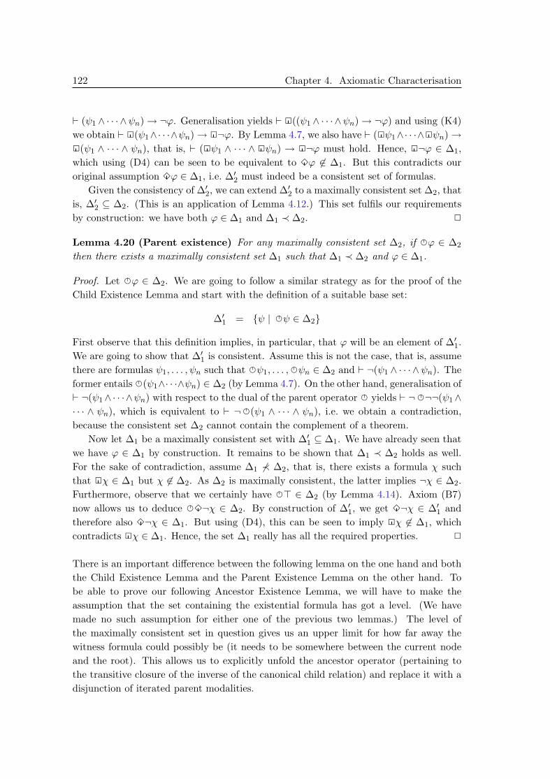
122 Chapter 4. Axiomatic Characterisation
` (ψ1 ∧ · · · ∧ψn) → ¬ϕ. Generalisation yields ` 2((ψ1 ∧ · · · ∧ψn) → ¬ϕ) and using (K4)we obtain ` 2(ψ1∧· · ·∧ψn) → 2¬ϕ. By Lemma 4.7, we also have ` (2ψ1∧· · ·∧2ψn) →2(ψ1 ∧ · · · ∧ ψn), that is, ` (2ψ1 ∧ · · · ∧ 2ψn) → 2¬ϕ must hold. Hence, 2¬ϕ ∈ ∆1,which using (D4) can be seen to be equivalent to 3ϕ 6∈ ∆1. But this contradicts ouroriginal assumption 3ϕ ∈ ∆1, i.e. ∆′
2 must indeed be a consistent set of formulas.Given the consistency of ∆′
2, we can extend ∆′2 to a maximally consistent set ∆2, that
is, ∆′2 ⊆ ∆2. (This is an application of Lemma 4.12.) This set fulfils our requirements
by construction: we have both ϕ ∈ ∆1 and ∆1 ≺ ∆2. 2
Lemma 4.20 (Parent existence) For any maximally consistent set ∆2, if eϕ ∈ ∆2
then there exists a maximally consistent set ∆1 such that ∆1 ≺ ∆2 and ϕ ∈ ∆1.
Proof. Let eϕ ∈ ∆2. We are going to follow a similar strategy as for the proof of theChild Existence Lemma and start with the definition of a suitable base set:
∆′1 = ψ | eψ ∈ ∆2
First observe that this definition implies, in particular, that ϕ will be an element of ∆′1.
We are going to show that ∆′1 is consistent. Assume this is not the case, that is, assume
there are formulas ψ1, . . . , ψn such that eψ1, . . . , eψn ∈ ∆2 and ` ¬(ψ1 ∧ · · · ∧ψn). Theformer entails e(ψ1∧· · ·∧ψn) ∈ ∆2 (by Lemma 4.7). On the other hand, generalisation of` ¬(ψ1∧· · ·∧ψn) with respect to the dual of the parent operator eyields ` ¬ e¬¬(ψ1∧· · · ∧ ψn), which is equivalent to ` ¬ e(ψ1 ∧ · · · ∧ ψn), i.e. we obtain a contradiction,because the consistent set ∆2 cannot contain the complement of a theorem.
Now let ∆1 be a maximally consistent set with ∆′1 ⊆ ∆1. We have already seen that
we have ϕ ∈ ∆1 by construction. It remains to be shown that ∆1 ≺ ∆2 holds as well.For the sake of contradiction, assume ∆1 6≺ ∆2, that is, there exists a formula χ suchthat 2χ ∈ ∆1 but χ 6∈ ∆2. As ∆2 is maximally consistent, the latter implies ¬χ ∈ ∆2.Furthermore, observe that we certainly have e> ∈ ∆2 (by Lemma 4.14). Axiom (B7)now allows us to deduce e3¬χ ∈ ∆2. By construction of ∆′
1, we get 3¬χ ∈ ∆′1 and
therefore also 3¬χ ∈ ∆1. But using (D4), this can be seen to imply 2χ 6∈ ∆1, whichcontradicts 2χ ∈ ∆1. Hence, the set ∆1 really has all the required properties. 2
There is an important difference between the following lemma on the one hand and boththe Child Existence Lemma and the Parent Existence Lemma on the other hand. Tobe able to prove our following Ancestor Existence Lemma, we will have to make theassumption that the set containing the existential formula has got a level. (We havemade no such assumption for either one of the previous two lemmas.) The level ofthe maximally consistent set in question gives us an upper limit for how far away thewitness formula could possibly be (it needs to be somewhere between the current nodeand the root). This allows us to explicitly unfold the ancestor operator (pertaining tothe transitive closure of the inverse of the canonical child relation) and replace it with adisjunction of iterated parent modalities.
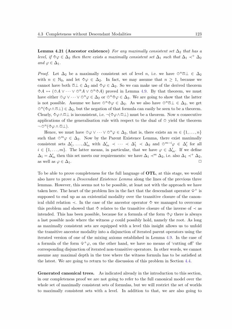
4.3 Completeness without Descendant Modalities 123
Lemma 4.21 (Ancestor existence) For any maximally consistent set ∆2 that has alevel, if 3ϕ ∈ ∆2 then there exists a maximally consistent set ∆1 such that ∆1 ≺+ ∆2
and ϕ ∈ ∆1.
Proof. Let ∆2 be a maximally consistent set of level n, i.e. we have en2⊥ ∈ ∆2
with n ∈ N0, and let 3ϕ ∈ ∆2. In fact, we may assume that n ≥ 1, because wecannot have both 2⊥ ∈ ∆2 and 3ϕ ∈ ∆2. So we can make use of the derived theorem3A ↔ ( eA ∨ · · · ∨ enA ∨ en3A) proved in Lemma 4.9. By that theorem, we musthave either eϕ ∨ · · · ∨ enϕ ∈ ∆2 or en3ϕ ∈ ∆2. We are going to show that the latteris not possible. Assume we have en3ϕ ∈ ∆2. As we also have en2⊥ ∈ ∆2, we geten(3ϕ∧2⊥) ∈ ∆2, but the negation of that formula can easily be seen to be a theorem.Clearly, 3ϕ∧2⊥ is inconsistent, i.e. ¬(3ϕ∧2⊥) must be a theorem. Now n consecutiveapplications of the generalisation rule with respect to the dual of e yield the theorem¬ en(3ϕ ∧2⊥).
Hence, we must have eϕ ∨ · · · ∨ enϕ ∈ ∆2, that is, there exists an m ∈ 1, . . . , nsuch that emϕ ∈ ∆2. Now by the Parent Existence Lemma, there exist maximallyconsistent sets ∆′
1, . . . ,∆′m with ∆′
m ≺ · · · ≺ ∆′1 ≺ ∆2 and em−iϕ ∈ ∆′
i for alli ∈ 1, . . . ,m. The latter means, in particular, that we have ϕ ∈ ∆′
m. If we define∆1 = ∆′
m then this set meets our requirements: we have ∆1 ≺m ∆2, i.e. also ∆1 ≺+ ∆2,as well as ϕ ∈ ∆1. 2
To be able to prove completeness for the full language of OTL, at this stage, we wouldalso have to prove a Descendant Existence Lemma along the lines of the previous threelemmas. However, this seems not to be possible, at least not with the approach we havetaken here. The heart of the problem lies in the fact that the descendant operator 3+ issupposed to end up as an existential modality over the transitive closure of the canon-ical child relation ≺. In the case of the ancestor operator 3 we managed to overcomethis problem and showed that 3 relates to the transitive closure of the inverse of ≺ asintended. This has been possible, because for a formula of the form 3ϕ there is alwaysa last possible node where the witness ϕ could possibly hold, namely the root. As longas maximally consistent sets are equipped with a level this insight allows us to unfoldthe transitive ancestor modality into a disjunction of iterated parent operators using theiterated version of one of the mixing axioms established in Lemma 4.9. In the case ofa formula of the form 3+ϕ, on the other hand, we have no means of ‘cutting off’ thecorresponding disjunction of iterated non-transitive operators. In other words, we cannotassume any maximal depth in the tree where the witness formula has to be satisfied atthe latest. We are going to return to the discussion of this problem in Section 4.4.
Generated canonical trees. As indicated already in the introduction to this section,in our completeness proof we are not going to refer to the full canonical model over thewhole set of maximally consistent sets of formulas, but we will restrict the set of worldsto maximally consistent sets with a level. In addition to that, we are also going to

124 Chapter 4. Axiomatic Characterisation
discard any sets that are not connected to some first set via an iteration of the canonicalchild relation and its inverse. This first set is said to generate the model. The followingdefinition makes precise the notion of a set of maximally consistent sets generated by agiven set ∆∗. In our Completeness Theorem at the end of this section, this set ∆∗ willbe the set containing the consistent formula in question and the corresponding world inthe (generated) canonical will be the world at which it will be shown to be satisfied.
Definition 4.22 (Generated set of maximally consistent sets) Let ∆∗ be a max-imally consistent set. We define T∆∗ as the set of maximally consistent sets ∆ for whichthere exist maximally consistent sets ∆1, . . . ,∆n with ∆1 = ∆∗ and ∆n = ∆ such thateither ∆i ≺ ∆i+1 or ∆i+1 ≺ ∆i for all natural numbers i < n.
In other words, T∆∗ is the set of worlds in the subframe generated by ∆∗ with respect tothe accessibility relation that is the union of ≺ and its inverse [13].
In Lemma 4.24 further below we are going to establish the first important resultabout the structure of the frame underlying our canonical model. The claim is thatT∆∗ , the set of maximally consistent sets generated by some maximally consistent set∆∗ (which will be required to have a level) and the canonical accessibility relation ≺from Definition 4.13 form a tree according to Definition 3.2. Amongst other things, thisinvolves proving that the canonical child relation ≺ is conversely functional, that is, anygiven maximally consistent set can have at most a single predecessor with respect to ≺.As this result does not depend on a restriction to maximally consistent sets with a level,we state it here as a lemma in its own right.
Lemma 4.23 (Converse functionality of canonical child relation) Let ∆, ∆1
and ∆2 be maximally consistent sets. Then ∆1 ≺ ∆ and ∆2 ≺ ∆ imply ∆1 = ∆2.
Proof. We are going to use the inverse axiom (B8): A → 2 eA and the functionalityaxiom (F3): eA ↔ (¬ e¬A ∧ e>). Let ∆, ∆1 and ∆2 be maximally consistent setswith ∆1 ≺ ∆ and ∆2 ≺ ∆. For the sake of contradiction, assume that ∆1 6= ∆2, i.e.there is a formula ϕ such that ϕ ∈ ∆1 and ¬ϕ ∈ ∆2. Application of modus ponens incombination with (B8) yields 2 eϕ ∈ ∆1 and 2 e¬ϕ ∈ ∆2. By definition of the relation≺, we get both eϕ ∈ ∆ and e¬ϕ ∈ ∆. From the former and the functionality axiom(F3) we can derive ¬ e¬ϕ ∈ ∆, i.e. we obtain a contradiction. Therefore, ∆1 and ∆2
must indeed be identical sets of formulas. 2
We are now ready to show that the order imposed by the canonical child relation overa set of maximally consistent sets generated by a given maximally consistent set with alevel must be a tree.
Lemma 4.24 (Generated canonical tree) Let ∆∗ be a maximally consistent set witha level. Then (T∆∗ ,≺) is a tree.

4.3 Completeness without Descendant Modalities 125
Proof. We need to show that ≺ is irreflexive and conversely functional over T∆∗ , andthat (T∆∗ ,≺) is rooted.
(1) Irreflexivity. ∆∗ is required to have a level. Hence, by Lemma 4.17 and thedefinition of T∆∗ , every set in T∆∗ must have a level, too. Irreflexivity of ≺ overT∆∗ can now be proved by contradiction. Assume there is a reflexive point, thatis, assume there exists a maximally consistent set ∆ ∈ T∆∗ with ∆ ≺ ∆. Because∆ must have a level, there exists an n ∈ N0 such that en2⊥ ∈ ∆. Furthermore,because we have ∆ ≺ ∆, Lemma 4.17 applies and we can infer en+12⊥ ∈ ∆ aswell. Now Lemma 4.16 on the uniqueness of levels yields n = n + 1, which is anobvious contradiction.
(2) Converse functionality. In Lemma 4.23 the relation ≺ has been shown to be con-versely functional over all maximally consistent sets, so it is certainly converselyfunctional over T∆∗ .
(3) Rootedness. The set ∆∗ is required to have a level, so there exists an m ∈ N suchthat em2⊥ ∈ ∆∗. Applying the Parent Existence Lemma m times proves thatthere must be a maximally consistent set ∆r with ∆r ≺m ∆∗ and 2⊥ ∈ ∆r. Thisset must be an element of T∆∗ . We are going to show that, in fact, ∆r is the(unique) root of (T∆∗ ,≺).
Recall that, according to Definition 4.22, for every ∆ ∈ T∆∗ there exist ∆1, . . . ,∆n
with ∆1 = ∆∗ and ∆n = ∆ such that either ∆i ≺ ∆i+1 or ∆i+1 ≺ ∆i for all i < n.This n provides us with a notion of ‘distance’ of a set ∆ from the generating set∆∗. We are going to prove, by induction over n, that for every ∆ ∈ T∆∗ we have∆r ≺∗ ∆. For the base case (n = 1), ∆ can only be ∆∗. Clearly, ∆r ≺∗ ∆∗ doeshold, because we have ∆r ≺m ∆∗. For the induction step, suppose the claim hasbeen shown to hold for all cases up to some natural number n. We have to show that∆r ≺∗ ∆ also holds for sets ∆ whose distance from ∆∗ is n+1. For such a ∆ theremust be a ∆n with either ∆n ≺ ∆ or ∆ ≺ ∆n for which the induction hypothesisholds, i.e. we have ∆r ≺∗ ∆n. In the case where ∆n ≺ ∆ holds, we immediatelyget ∆r ≺∗ ∆ as well and are done. So suppose ∆ ≺ ∆n. As we have ∆r ≺∗ ∆n,we have either ∆r ≺+ ∆n or ∆r = ∆n. But the latter would entail that ∆ ≺ ∆r,which would contradict Lemma 4.18. Hence, ∆r ≺+ ∆n will hold, which meanswe immediately get ∆r ≺∗ ∆ and are done. This concludes our inductive prooffor T∆∗ ⊆ ∆ | ∆r ≺∗ ∆. The other direction, namely ∆ | ∆r ≺∗ ∆ ⊆ T∆∗ ,is an immediate consequence of the definition of T∆∗ and the fact that ∆r ∈ T∆∗ .Hence, we have T∆∗ = ∆ | ∆r ≺∗ ∆, which means that ∆r is a root of (T∆∗ ,≺).
We still have to show that ∆r is a unique root element. As we have 2⊥ ∈ ∆r, byLemma 4.18, there can be no maximally consistent set ∆ with ∆ ≺ ∆r. So thereis certainly no maximally consistent set in T∆∗ different from ∆r from which ∆r
itself is accessible via the transitive closure of ≺. But this would be a necessaryrequirement for any root node of (T∆∗ ,≺), so the root ∆r is indeed unique.

126 Chapter 4. Axiomatic Characterisation
This concludes our proof of Lemma 4.24 as we have verified all conditions set out inDefinition 3.2 for an arbitrary relation to be a tree. 2
We note that we have not made any reference to the proposed rootedness axiom (R1),which involves the descendant operator 3+, in this proof. In fact, we are only going touse (R1) in the next section where we are going to analyse the problems related to theaxiomatisation of the descendant operator in some more detail.
Horizontal accessibility relations. We now turn to the horizontal dimension ofour canonical model. In the following definition we introduce two horizontal accessibilityrelation over maximally consistent sets of formulas in a similar manner as we have definedthe canonical child relation ≺. Or aim later on will be to show that these two newrelations correspond to the pseudo sibling relation S and the pseudo neighbour relationN of a loosely ordered tree, respectively.
Definition 4.25 (Canonical sibling and neighbour relations) Let ∆1 and ∆2 bemaximally consistent sets. We define the canonical sibling relation < and the canonicalneighbour relation < over maximally consistent sets as follows:
∆1 < ∆2 iff 2ϕ ∈ ∆1 implies ϕ ∈ ∆2 for all formulas ϕ∆1 < ∆2 iff e> ∈ ∆1 and eϕ ∈ ∆1 implies ϕ ∈ ∆2 for all formulas ϕ
Transitive closures of < and < will be denoted in accordance with Definition A.3 fromAppendix A. The relation <+
, for instance, is the non-reflexive transitive closure of<. The following lemma is the horizontal counterpart to Lemma 4.14. It states thatmaximally consistent sets are ‘aware’ of their predecessors and successors with respectto the canonical sibling and neighbour relations.
Lemma 4.26 (Horizontal awareness) Let ∆1 and ∆2 be maximally consistent setsand let ϕ be a formula. Then the following statements are true:
(1) ϕ ∈ ∆1 and ∆1 < ∆2 imply 3ϕ ∈ ∆2.
(2) ϕ ∈ ∆2 and ∆1 < ∆2 imply 3ϕ ∈ ∆1.
(3) ϕ ∈ ∆1 and ∆1 < ∆2 imply eϕ ∈ ∆2.
(4) ϕ ∈ ∆2 and ∆1 < ∆2 imply eϕ ∈ ∆1.
Proof. The four claims follow almost immediately from the definitions of < and <,respectively, together with some of the basic inverse, duality, and functionality axioms.
(1) Left sibling awareness. Let ϕ ∈ ∆1 and ∆1 < ∆2. Using the inverse axiom (B2),we can infer 23ϕ ∈ ∆1 and hence, by definition of <, we have 3ϕ ∈ ∆2.

4.3 Completeness without Descendant Modalities 127
(2) Right sibling awareness. Let ϕ ∈ ∆2 and ∆1 < ∆2. For the sake of contradiction,assume 3ϕ 6∈ ∆1, which by (D2) is equivalent to 2¬ϕ ∈ ∆1. By definition of<, the latter entails ¬ϕ ∈ ∆2, the contradiction we have been looking for. Thus3ϕ ∈ ∆1 as claimed.
(3) Left neighbour awareness. Let ϕ ∈ ∆1 and ∆1 < ∆2. The latter implies inparticular e> ∈ ∆1. Hence, axiom (B6) is applicable and we can infer e eϕ ∈ ∆1.Then eϕ ∈ ∆2 follows by definition of <.
(4) Right neighbour awareness. Let ϕ ∈ ∆2 and ∆1 < ∆2. For the sake of contradic-tion, assume eϕ ∈ ∆1 is not the case. Then ¬ e¬¬ϕ ∈ ∆1 must be true. Becauseof ∆1 < ∆2, we also have e> ∈ ∆1 and thus may use the functionality axiom(F2) in order to obtain e¬ϕ ∈ ∆1. By definition of <, this implies ¬ϕ ∈ ∆2,which contradicts our original assumption ϕ ∈ ∆2. Hence, eϕ ∈ ∆1 must be thecase.
This completes our proof of Lemma 4.26. 2
Horizontal existence lemmas. In analogy to our vertical Existence Lemmas provedearlier, we now have to show that also for the existential operators pertaining to thecanonical sibling and the canonical neighbour relation, there will always be a related setcontaining an appropriate witness formula.
Lemma 4.27 (Right sibling existence) For any maximally consistent set ∆1, if3ϕ ∈ ∆1 then there exists a maximally consistent set ∆2 such that ∆1 < ∆2 and ϕ ∈ ∆2.
Proof. Let 3ϕ ∈ ∆1. We start by constructing a set ∆′2 containing all those formulas
that are ‘forced’ to belong to any <-successor of ∆1:
∆′2 = ϕ ∪ ψ | 2ψ ∈ ∆1
The consistency of ∆′2 can be proved by contradiction. If it is not consistent, then
there must be formulas ψ1, . . . , ψn such that 2ψi ∈ ∆1 for all i ∈ 1, . . . , n and `¬(ψ1 ∧ · · · ∧ ψn ∧ ϕ). The former implies 2(ψ1 ∧ · · · ∧ ψn) ∈ ∆1 (by Lemma 4.7). Thelatter is equivalent to ` (ψ1 ∧ · · · ∧ ψn) → ¬ϕ. If we apply the generalisation rule, weget ` 2((ψ1 ∧ · · · ∧ ψn) → ¬ϕ) and then, using axiom (K2), ` 2(ψ1 ∧ · · · ∧ ψn) → 2¬ϕ.Hence, 2¬ϕ ∈ ∆1. But an application of axiom (D2) shows that this is equivalent to3ϕ 6∈ ∆1, that is, we have derived a contradiction and ∆′
2 must be a consistent set offormulas.
Therefore, by Lemma 4.12, we can extend ∆′2 to a maximally consistent set ∆2. We
have ϕ ∈ ∆2 by construction and also ∆1 < ∆2, because for every formula of the form2ψ in ∆1 its principal subformula ψ will be in ∆′
2, and thereby also in ∆2. 2
Lemma 4.28 (Left sibling existence) For any maximally consistent set ∆2, if 3ϕ ∈∆2 then there exists a maximally consistent set ∆1 such that ∆1 < ∆2 and ϕ ∈ ∆1.

128 Chapter 4. Axiomatic Characterisation
Proof. This can be shown in direct analogy to the proof of Lemma 4.27. 2
Lemma 4.29 (Right neighbour existence) For any maximally consistent set ∆1, ifeϕ ∈ ∆1 then there exists a maximally consistent set ∆2 such that ∆1 < ∆2 andϕ ∈ ∆2.
Proof. Let eϕ ∈ ∆1. As before, our first step is to construct a (consistent) set ∆′2 of
formulas that are forced to belong to any set ∆2 that could fulfil the conditions of theclaim, i.e. that could act as a righthand neighbour for the set ∆1.
∆′2 = ψ | eψ ∈ ∆1
We prove that ∆′2 is consistent. For ∆′
2 to be inconsistent there would have to be formulasψ1, . . . , ψn with eψ1, . . . , eψ ∈ ∆1 and ` ¬(ψ1∧· · ·∧ψn). If we apply the generalisationrule with respect to ¬ e¬ to the latter, we obtain ` ¬ e¬¬(ψ1 ∧ · · · ∧ψn). On the otherhand, as we can distribute the right neighbour operator, the formula e(ψ1 ∧ · · · ∧ ψn)must belong to ∆1, which is a contradiction. Hence, ∆′
2 must be a consistent set offormulas and can be extended to a maximally consistent set ∆2.
We have ϕ ∈ ∆2 by construction. Furthermore, ∆1 < ∆2 must hold as well, becausewe have ψ ∈ ∆2 for every eψ ∈ ∆1, and e> ∈ ∆1, which follows from eϕ ∈ ∆1 andaxiom (F2). 2
Lemma 4.30 (Left neighbour existence) For any maximally consistent set ∆2, ifeϕ ∈ ∆2 then there exists a maximally consistent set ∆1 such that ∆1 < ∆2 andϕ ∈ ∆1.
Proof. This can be proved in the same way as Lemma 4.29. 2
Properties of the canonical frame. In the following sequence of lemmas we shallestablish a number of properties of the relations ≺, < and < declared over maximallyconsistent sets of formulas. As will be made precise later on, (most of) these propertiescorrespond to the properties of loosely ordered trees listed in Definition 3.33. In orderto emphasise the correspondences between the semantic and the axiomatic level, at thebeginning of each of the proofs, we shall quote the central axiom(s) used to prove therespective property.
In the proof of Lemma 4.42 (on page 134) we are going to summarise these resultsand show that the frame which our canonical accessibility relations give rise to must bea loosely ordered tree.
Lemma 4.31 (Transitivity of canonical sibling relation) The relation < declaredover maximally consistent sets is transitive.
Proof. We are going to use axiom (H1): 2A → 22A. Suppose ∆1, ∆2 and ∆3 aremaximally consistent sets such that ∆1 < ∆2 and ∆2 < ∆3. We need to show that

4.3 Completeness without Descendant Modalities 129
∆1 < ∆3 holds as well, that is, we need to show that 2ϕ ∈ ∆1 implies ϕ ∈ ∆3 for anygiven formula ϕ. So let 2ϕ ∈ ∆1. By axiom (H1), this implies 22ϕ ∈ ∆1. Now, using∆1 < ∆2, we obtain 2ϕ ∈ ∆2, and then, using ∆2 < ∆3, we get the required resultϕ ∈ ∆3. 2
Lemma 4.32 (Common parents of siblings) Let ∆1 and ∆2 be maximally consis-tent sets with ∆1 < ∆2. Then there exists a maximally consistent set ∆ such that∆ ≺ ∆1 and ∆ ≺ ∆2.
Proof. We are going to use the interaction axiom (X1): 3A → e3A. Let ∆1 and ∆2
be maximally consistent sets such that ∆1 < ∆2. According to Lemma 4.26, the set ∆1
will be ‘aware’ of its successor, that is, we must have 3> ∈ ∆1. By axiom (X1), we thenalso have e3> ∈ ∆1. Hence, by the Parent Existence Lemma, there exists a maximallyconsistent set ∆ with ∆ ≺ ∆1 (and 3> ∈ ∆, but this second conclusion is not of interesthere).
To show that ∆ ≺ ∆2 holds as well, we are going to use theorem 2A→ 22A, whichhas been proved correct in Lemma 4.8.10 Let ϕ be a formula with 2ϕ ∈ ∆. Using2A→ 22A yields 22ϕ ∈ ∆. This implies 2ϕ ∈ ∆1, because we have ∆ ≺ ∆1. This inturn implies ϕ ∈ ∆2, because we have ∆1 < ∆2. Thus ∆ ≺ ∆2, because we have shownthat 2ϕ ∈ ∆ implies ϕ ∈ ∆2 for all formulas ϕ. 2
Lemma 4.33 (Connectedness of children) Let ∆, ∆1 and ∆2 be maximally consis-tent sets with ∆ ≺ ∆1 and ∆ ≺ ∆2. Then we must have either ∆1 = ∆2 or ∆1 < ∆2 or∆2 < ∆1.
Proof. The central axiom for this proof will be the second interaction axiom (X2):e3A → (A ∨ 3A ∨ 3A). Let ∆ ≺ ∆1 and ∆ ≺ ∆2. For the sake of contradiction,assume that neither ∆1 = ∆2 nor ∆1 < ∆2 nor ∆2 < ∆1 holds. Then there must beformulas ϕ, χ and ψ such that ϕ ∈ ∆1 but ϕ 6∈ ∆2 (otherwise ∆1 = ∆2), 2χ ∈ ∆1 butχ 6∈ ∆2 (otherwise ∆1 < ∆2), and 2ψ ∈ ∆2 but ψ 6∈ ∆1 (otherwise ∆2 < ∆1).
Because ∆2 is maximally consistent, we also have ¬ϕ ∧ ¬χ ∧2ψ ∈ ∆2. We can nowapply Lemma 4.14, first to deduce 3(¬ϕ ∧ ¬χ ∧ 2ψ) ∈ ∆ (using ∆ ≺ ∆2) and then toobtain e3(¬ϕ ∧ ¬χ ∧2ψ) ∈ ∆1 (using ∆ ≺ ∆1). Now axiom (X2) can be used to inferthat we must have either (1) ¬ϕ ∧ ¬χ ∧ 2ψ ∈ ∆1 or (2) 3(¬ϕ ∧ ¬χ ∧ 2ψ) ∈ ∆1 or (3)3(¬ϕ∧¬χ∧2ψ) ∈ ∆1. But as we shall see, each one of these three options will lead toa contradiction.
(1) ¬ϕ ∧ ¬χ ∧2ψ ∈ ∆1 directly contradicts our assumption ϕ ∈ ∆1.
(2) If 3(¬ϕ ∧ ¬χ ∧2ψ) ∈ ∆1 is the case, then by the Left Sibling Lemma there mustbe a maximally consistent set ∆′ such that ∆′ < ∆1 and ¬ϕ∧¬χ∧2ψ ∈ ∆′. Thisimplies in particular 2ψ ∈ ∆′. Hence, by definition of <, we get ψ ∈ ∆1, whichcontradicts our earlier assumption ψ 6∈ ∆1.
10In fact, the proof given in Lemma 4.8 shows that 2A→ 22A essentially follows from (X1). So (X1)
really is the central axiom here.

130 Chapter 4. Axiomatic Characterisation
(3) Now the only remaining option is 3(¬ϕ ∧ ¬χ ∧ 2ψ) ∈ ∆1. By the Right SiblingExistence Lemma there exists a maximally consistent set ∆′ with ∆1 < ∆′ and¬ϕ ∧ ¬χ ∧ 2ψ ∈ ∆′, which implies in particular ¬χ ∈ ∆′. But we also have2χ ∈ ∆1 and therefore χ ∈ ∆′, that is, we have again encountered a contradiction.
Hence, our assumption that neither ∆1 = ∆2 nor ∆1 < ∆2 nor ∆2 < ∆1 holds is indeedcontradictory and we are done. 2
The following two lemmas do not themselves correspond to properties of loosely orderedtrees specifically postulated by Definition 3.33, but are simple consequences of thoseconditions. We explicitly state them here in order to simplify the presentation of theproofs of some of our later lemmas.
Lemma 4.34 (No branching to the right) Let ∆, ∆1 and ∆2 be maximally consis-tent sets such that ∆ < ∆1 and ∆ < ∆2. Then we have either ∆1 = ∆2 or ∆1 < ∆2 or∆2 < ∆1.
Proof. Let ∆, ∆1 and ∆2 be maximally consistent sets such that ∆ < ∆1 and ∆ < ∆2.Because of the former, by Lemma 4.32, there must be a maximally consistent set ∆p
such that ∆p ≺ ∆ and ∆p ≺ ∆1. We can apply Lemma 4.32 a second time and inferthat there must also be a maximally consistent set ∆′
p with ∆′p ≺ ∆ and ∆′
p ≺ ∆2. But≺ has been shown to be a conversely functional relation in Lemma 4.23, so we must have∆p = ∆′
p, as these sets are both predecessors of the same set ∆. We can now see thatthere exists a maximally consistent set, namely ∆p, that is a predecessor (with respect to≺) to both ∆1 and ∆2. In other words, we have both ∆p ≺ ∆1 and ∆p ≺ ∆2. Therefore,Lemma 4.33 is applicable, that is, we must have either ∆1 = ∆2 or ∆1 < ∆2 or ∆2 < ∆1
as claimed. 2
Lemma 4.35 (No branching to the left) Let ∆, ∆1 and ∆2 be maximally consistentsets such that ∆1 < ∆ and ∆2 < ∆. Then we have either ∆1 = ∆2 or ∆1 < ∆2 or∆2 < ∆1.
Proof. Omitted. The proof would be almost identical to that of Lemma 4.34. 2
Lemma 4.36 (Functionality of canonical neighbour relations) Both < and itsinverse as declared over maximally consistent sets are functional relations.
Proof. For the two parts of this proof, we are going to make use of axioms (F2): eA↔(¬ e¬A ∧ e>) and (F1): eA↔ (¬ e¬A ∧ e>), respectively.
We first show that < is a functional relation. Let ∆, ∆1 and ∆2 be maximallyconsistent sets of formulas with ∆ < ∆1 and ∆ < ∆2. Functionality of < wouldthen imply ∆1 = ∆2. So for the sake of contradiction, assume this is not the case, i.e.there exists a formula ϕ with ϕ ∈ ∆1 and ¬ϕ ∈ ∆2. By Lemma 4.26, the former entails

4.3 Completeness without Descendant Modalities 131
eϕ ∈ ∆, while the latter implies e¬ϕ ∈ ∆. But from (F2) and eϕ ∈ ∆ we can infer¬ e¬ϕ ∈ ∆, that is, we have derived a contradiction.
Let us now turn to the second part of the claim. Suppose ∆, ∆1 and ∆2 are maximallyconsistent sets such that ∆1 < ∆ and ∆2 < ∆. To prove that the inverse of < isa functional relation, we are going to show that the assumption ∆1 6= ∆2 leads to acontradiction. By this assumption, there must be a formula ϕ with ϕ ∈ ∆1 and ¬ϕ ∈ ∆2.We apply again Lemma 4.26 and get eϕ ∈ ∆ and e¬ϕ ∈ ∆. The former together with(F1) gives us ¬ e¬ϕ ∈ ∆, which contradicts e¬ϕ ∈ ∆. 2
Lemma 4.37 (Neighbours and siblings) Let ∆1 and ∆2 be maximally consistentsets. Then ∆1 < ∆2 implies ∆1 < ∆2.
Proof. We are going to use theorem (2A ∧ e>) → eA from Lemma 4.8, whosederivation crucially depended on axiom (M2). Let ∆1 and ∆2 be maximally consistentsets such that ∆1 < ∆2 holds. To show that ∆1 < ∆2 must be true as well, we haveto show that 2ϕ ∈ ∆1 implies ϕ ∈ ∆2 for all formulas ϕ. So let 2ϕ ∈ ∆1. Because of∆1 < ∆2, we also have e> ∈ ∆1. That means we can apply theorem (2A∧ e>) → eAand get eϕ ∈ ∆1. Now ∆1 < ∆2 entails ϕ ∈ ∆2 by definition of <. 2
The following is another auxiliary lemma.
Lemma 4.38 (Composed canonical sibling relation) Let ∆1 and ∆2 be maximallyconsistent sets. Then ∆1 <
2 ∆2 holds iff 22ϕ ∈ ∆1 implies ϕ ∈ ∆2 for all formulas ϕ.
Proof. ‘⇒’: This is the easy part. Let ∆1 and ∆2 be maximally consistent sets with∆1 <
2 ∆2, that is, there exists a maximally consistent set ∆ such that ∆1 < ∆ and∆ < ∆2. Now assume 22ϕ ∈ ∆1. By definition of < we first get 2ϕ ∈ ∆ and thenϕ ∈ ∆2 as claimed.
‘⇐’: Now let ∆1 and ∆2 be such that 22ϕ ∈ ∆1 implies ϕ ∈ ∆2 for all formulas ϕ.To prove that this implies ∆1 <
2 ∆2 we are going to show that there exists a maximallyconsistent set ∆ such that ∆1 < ∆ and ∆ < ∆2 are true. We first construct a base set∆′ containing all the formulas that can immediately be seen to be required to be part ofany such set ‘between’ ∆1 and ∆2:
∆′ = χ | 2χ ∈ ∆1 ∪ 3ψ | ψ ∈ ∆2
We claim that ∆′ is a consistent set of formulas. Otherwise there would have to beformulas χ1, . . . , χn with 2χi ∈ ∆1 for all i ∈ 1, . . . , n and formulas ψ1, . . . , ψm ∈ ∆2
such that ` ¬(χ1 ∧ · · · ∧ χn ∧ 3ψ1 ∧ · · · ∧ 3ψm) holds. This can be seen to lead to acontradiction as follows. We can transform the previous statement into ` (χ1∧· · ·∧χn) →(¬3ψ1 ∨ · · · ∨ ¬3ψm) and then use the generalisation rule and axiom (K2) to obtain` 2(χ1 ∧ · · · ∧ χn) → 2(¬3ψ1 ∨ · · · ∨ ¬3ψm). Hence, as we have 2(χ1 ∧ · · · ∧ χn) ∈ ∆1
(by distribution), we must also have 2(¬3ψ1 ∨ · · · ∨ ¬3ψm) ∈ ∆1. By axiom (D2)

132 Chapter 4. Axiomatic Characterisation
this is equivalent to 2(2¬ψ1 ∨ · · · ∨ 2¬ψm) ∈ ∆1, which in turn is easily seen to imply22(¬ψ1 ∨ · · · ∨¬ψm) ∈ ∆1.11 Together with our original assumption of 22ϕ ∈ ∆1
implying ϕ ∈ ∆2 for all formulas ϕ, this entails ¬ψ1 ∨ · · · ∨¬ψm ∈ ∆2. But thiscontradicts ψ1, . . . , ψm ∈ ∆2.
Thus ∆′ must be consistent and, by Lemma 4.12, we can extend it to a maximallyconsistent set ∆. We have ∆1 < ∆ by construction and ∆ < ∆2 must hold as well,because ¬ϕ ∈ ∆2 implies 3¬ϕ ∈ ∆ (which is equivalent to ¬2ϕ ∈ ∆), again, byconstruction. Hence, ∆1 <
2 ∆2 holds as claimed. 2
Lemma 4.39 (Direct siblings and neighbours) Let ∆1 and ∆2 be maximally con-sistent sets with ∆1 < ∆2 and suppose there exists no maximally consistent set ∆ suchthat both ∆1 < ∆ and ∆ < ∆2 hold. Then we must have ∆1 < ∆2.
Proof. The proof will employ axiom (H2): 22A→ (2A∨ e>). Suppose ∆1 and ∆2 aremaximally consistent sets as specified in the claim, that is, we have ∆1 < ∆2 and thereis no maximally consistent set ∆ such that ∆1 < ∆ and ∆ < ∆2. We are first goingto show that there exists a maximally consistent set ∆′
2 such that ∆1 < ∆′2 holds and
then that, in fact, we must have ∆′2 = ∆2 for any such set.
For the sake of contradiction, assume there exists no ∆′2 such that ∆1 < ∆′
2. Bythe Right Neighbour Existence Lemma, this implies e> 6∈ ∆1. We are going to deriveour contradiction by showing that under these conditions there will be a ∆ such that∆1 < ∆ < ∆2. According to Lemma 4.38, this is the case iff 22ϕ ∈ ∆1 implies ϕ ∈ ∆2
for every formula ϕ. So let 22ϕ ∈ ∆1. Now axiom (H2) applies and we can concludethat the disjunction 2ϕ ∨ e> must also be an element of ∆1. Together with e> 6∈ ∆1
this entails 2ϕ ∈ ∆1. But then ∆1 < ∆2 entails ϕ ∈ ∆2, that is, we have indeed founda contradiction.
Hence, there exists a maximally consistent set ∆′2 with ∆1 < ∆′
2. By Lemma 4.37,< is a subrelation to <, that is, we also have ∆1 < ∆′
2. Applying Lemma 4.34 to thelatter and ∆1 < ∆2 allows us to infer that either ∆2 = ∆′
2 or ∆2 < ∆′2 or ∆′
2 < ∆2 mustbe true. We have to exclude the latter two cases. In fact, ∆′
2 < ∆2 is immediately seento be contradictory, as in that case we would have a maximally consistent set ∆, namely∆′
2, such that ∆1 < ∆ < ∆2 (and this possibility is explicitly excluded in the claim).So it remains to be shown that the assumption ∆2 < ∆′
2 also leads to a contradiction.We are again going to make use of the original assumption that there is no maximallyconsistent set ∆ such that ∆1 < ∆ < ∆2. Again, by Lemma 4.38, this is the same asto say that there exists a formula ϕ such that 22ϕ ∈ ∆1 but ϕ 6∈ ∆2. The formertogether with ∆1 < ∆2 < ∆′
2 yields ϕ ∈ ∆′2. Furthermore, ϕ 6∈ ∆2 and ∆1 < ∆2 entail
3¬ϕ ∈ ∆1. We also have e> ∈ ∆1 because of ∆1 < ∆′2. Now we can apply axiom (M2):
11Here is a sketch for a formal derivation: ¬ψ1 implies the disjunction ¬ψ1 ∨ · · · ∨¬ψm. Using the
generalisation rule and axiom (K2) we can see that therefore also 2¬ψ1 implies 2(¬ψ1 ∨ · · · ∨¬ψm). By
the same argument, 2¬ψi implies 2(¬ψ1 ∨ · · · ∨¬ψm) for all i ∈ 1, . . . ,m. Hence, 2¬ψ1 ∨ · · · ∨2¬ψm
implies 2(¬ψ1 ∨ · · · ∨¬ψm). Applying the generalisation rule and axiom (K2) once more then yields the
desired result.

4.3 Completeness without Descendant Modalities 133
•∆1
(2) e2ϕ from (1)(3) 22ϕ from (2)(7) e(ϕ ∧2ϕ) from (6)(8) 2ϕ from (7)
• ∆2
(1) 2ϕ assumption(5) ϕ from (4)(6) ϕ ∧2ϕ from (1) and (5)
•∆3
(4) 2ϕ from (3)(9) ϕ from (8)
Given: ∆1 < ∆2 and ∆1 < ∆3
Furthermore, assume: ∆3 < ∆2
Show: 2ϕ ∈ ∆2 implies ϕ ∈ ∆3,that is, show: ∆2 < ∆3
<
99
<11
<
##
Z W U R O LH
Figure 4.1: Proof detail for Lemma 4.40
(3A∧ e>) ↔ ( eA∨ e3A), that is, we must have either e¬ϕ ∈ ∆1 or e3¬ϕ ∈ ∆1. Bythe Right Neighbour Existence Lemma and the fact that < is known to be a functionalrelation (Lemma 4.36), the former contradicts ϕ ∈ ∆′
2. By the same argument, the latterimplies 3¬ϕ ∈ ∆′
2. But then, because of ∆1 < ∆′2, we have 33¬ϕ ∈ ∆1. This can be
seen to contradict 22ϕ ∈ ∆1 using axiom (D2). In summary, this means we have shownthat ∆2 = ∆′
2 is the only remaining case, that is, ∆1 < ∆2 must hold as claimed. 2
Lemma 4.40 (Right siblings of left neighbours) Let ∆1, ∆2 and ∆3 be maximallyconsistent sets such that ∆1 < ∆2 and ∆1 < ∆3. Then we must have either ∆2 = ∆3
or ∆2 < ∆3.
Proof. We are going to use the derived theorems e2A → 22A and e(A ∧ 2A) → 2A
from Lemma 4.8, the derivation of which particularly relied on axioms (M2) and (F2).Let ∆1, ∆2 and ∆3 be maximally consistent sets such that ∆1 < ∆2 and ∆1 < ∆3. ByLemma 4.37, the former implies ∆1 < ∆2. Hence, we can apply Lemma 4.34 to inferthat ∆2 = ∆3 or ∆2 < ∆3 or ∆3 < ∆2. If either ∆2 = ∆3 or ∆2 < ∆3 is the case we aredone, so let us assume ∆3 < ∆2. We are going to prove that ∆2 < ∆3 must be true aswell, by showing that 2ϕ ∈ ∆2 implies ϕ ∈ ∆3 for any formula ϕ. So let 2ϕ ∈ ∆2. Thereader may find it helpful to refer to Figure 4.1 when following this part of the argument.
By Lemma 4.26, we have e2ϕ ∈ ∆1 (because of ∆1 < ∆2) and we can use theoreme2A → 22A to obtain 22ϕ ∈ ∆1. Thus we also get 2ϕ ∈ ∆3 and then ϕ ∈ ∆2
(because of ∆1 < ∆3 < ∆2). Now we have e(ϕ ∧ 2ϕ) ∈ ∆1 and can apply theoreme(A ∧2A) → 2A to obtain 2ϕ ∈ ∆1. Hence, ϕ ∈ ∆3 must hold (because of ∆1 < ∆3),which is what we intended to derive. So at least one of ∆2 = ∆3 and ∆2 < ∆3 will betrue in any case. 2
Lemma 4.41 (Left siblings of right neighbours) Let ∆1, ∆2 and ∆3 be maximallyconsistent sets such that ∆1 < ∆3 and ∆2 < ∆3. Then we must have either ∆1 = ∆2
or ∆1 < ∆2.

134 Chapter 4. Axiomatic Characterisation
•∆2
(4) e2¬ e¬ϕ from (3)(5) 22¬ e¬ϕ from (4)(9) ϕ from (8)
• ∆3
(3) 2¬ e¬ϕ from (2)(7) ¬ e¬ϕ from (6)(8) eϕ from (7)
•∆1
(1) 2ϕ assumption(2) 22¬ e¬ϕ from (1)(6) 2¬ eϕ from (5)
Given: ∆2 < ∆3 and ∆1 < ∆3
Furthermore, assume: ∆2 < ∆1
Show: 2ϕ ∈ ∆1 implies ϕ ∈ ∆2,that is, show: ∆1 < ∆2
<
99
<
##
<11
vr
o l i g d
Figure 4.2: Proof detail for Lemma 4.41
Proof. The structure of this proof is similar to that of the previous lemma. This time weare going to use axiom (H3): 2A → 22¬ e¬A and the derived theorem e2A → 22A
from before. Let ∆1, ∆2 and ∆3 be maximally consistent sets with ∆1 < ∆3 and∆2 < ∆3. The latter implies ∆2 < ∆3 and we can apply Lemma 4.35 to see that either∆1 = ∆2 or ∆1 < ∆2 or ∆2 < ∆1. We are done if we can prove that ∆2 < ∆1 implies∆1 < ∆2. So assume ∆2 < ∆1 and 2ϕ ∈ ∆1. (We need to show ϕ ∈ ∆2.) The followingargument is also summarised in Figure 4.2.
Axiom (H3) together with 2ϕ ∈ ∆1 entails 22¬ e¬ϕ ∈ ∆1. Now we obtainfirst 2¬ e¬ϕ ∈ ∆3 (because of ∆1 < ∆3) and then e2¬ e¬ϕ ∈ ∆2 (because of∆2 < ∆3). At this point theorem e2A → 22A applies and we get 22¬ e¬ϕ ∈ ∆2
as well. Because of ∆2 < ∆1 < ∆3 we then get ¬ e¬ϕ ∈ ∆3. As we certainly havee> ∈ ∆3 (from ∆2 < ∆3 and Lemma 4.26), the functionality axiom (F1) allowsus to infer eϕ ∈ ∆3. Hence, by the Left Neighbour Existence Lemma and the factthat the inverse of< is a functional relation (Lemma 4.36) we get ϕ ∈ ∆2 as required. 2
We are now ready to put together our results on properties of the structure imposedon the set of maximally consistent sets with a level by the three canonical accessibilityrelations ≺, < and <.
Lemma 4.42 (Generated canonical loosely ordered trees) Let ∆∗ be a maxi-mally consistent set with a level. Then (T∆∗ ,≺, <,<) is a loosely ordered tree.
Proof. Let ∆∗ be a maximally consistent set with a level, that is, ∆∗ contains a formulaof the form en2⊥. Then T∆∗ is the set of maximally consistent sets generated by ∆∗.That is, any maximally consistent set that can be reached from ∆∗ via a composition (ofarbitrary length) of the relation ≺ and its inverse will belong to T∆∗ (see Definition 4.22).Part of the claim of this lemma is that the sets in T∆∗ are in fact nodes in a loosely orderedtree and that ≺ is the child relation for that tree. Furthermore, < is claimed to be the

4.3 Completeness without Descendant Modalities 135
corresponding pseudo sibling relation and < is claimed to be the pseudo neighbourrelation.
To prove this, we have to check the nine conditions from Definition 3.33. These haveall been shown to hold in earlier lemmas; we merely need to summarise:
(1) By Lemma 4.24, (T∆∗ ,≺) is a tree.
(2) By Lemma 4.31, < is a transitive relation.
(3) By Lemma 4.32, any two nodes related via< will also be related via the compositionof the inverse of ≺ and ≺ itself.
(4) By Lemma 4.33, any two nodes related via the composition of the inverse of ≺ and≺ itself will also be related via either the reflexive closure or the inverse of <.
(5) By Lemma 4.36, both < and its inverse are functional relations.
(6) By Lemma 4.37, any two nodes related via < will also be related via <.
(7) By Lemma 4.39, any two nodes related via < but not via the composition of <with itself will also be related via <.
(8) By Lemma 4.40, any two nodes related via the composition of the inverse of <and < will also be related via the reflexive closure of <.
(9) By Lemma 4.41, any two nodes related via the composition of < and the inverseof < will also be related via the reflexive closure of <.
This concludes our proof of Lemma 4.42 2
Generated canonical models. The canonical relations ≺, < and < from Defini-tions 4.13 and 4.25 are all binary relations over the full set of maximally consistent sets.So they are also relations over the set of maximally consistent sets T∆∗ generated bysome set ∆∗ (see Definition 4.22) and we may speak about a frame (T∆∗ ,≺, <,<) inthe sense of Definition 3.16.
Definition 4.43 (Generated canonical frames) Let ∆∗ be a maximally consistentset with a level. Then the general frame F∆∗ = (T∆∗ ,≺, <,<) is called the canonicalframe generated by ∆∗.
Next we define a canonical valuation to go with our generated canonical frames. Thisis going to be a function mapping propositional letters to sets of maximally consistentsets of formulas (the ‘worlds’ in our canonical model to be). A propositional letter P isintended to be true at a world represented by a maximally consistent set ∆ iff P is anelement of ∆. Our valuation function is defined accordingly.

136 Chapter 4. Axiomatic Characterisation
Definition 4.44 (Generated canonical valuations) Let ∆∗ be a maximally consis-tent set with a level. The function V∆∗ from the set of propositional letters to the gen-erated set of maximally consistent sets T∆∗, with V∆∗(P ) = ∆ ∈ T∆∗ | P ∈ ∆ forpropositional letters P , is called the valuation function generated by ∆∗.
Finally, we can give a formal definition of our canonical models.
Definition 4.45 (Generated canonical models) Let ∆∗ be a maximally consistentset with a level. Then the general model M∆∗ = (F∆∗ , V∆∗), is called the canonicalmodel generated by ∆∗.
Truth in canonical models. After having established that our canonical frames haveall the required properties (i.e. they are loosely ordered trees) and after having provedExistence Lemmas for the various existential modalities in our language, the last im-portant step to take before we can formulate our completeness result is to prove anappropriate Truth Lemma. We have to show that the notion of truth in a generatedcanonical model (in the sense of Definition 3.18) coincides with our intended notion oftruth, which simply reduces to membership in the respective maximally consistent set.In other words, a formula should be true at a world in a generated canonical model iffthat formula is an element of the maximally consistent set of formulas associated withthat world.
The following lemma is the first instance where we explicitly have to exclude thetransitive descendant modalities 3+ and 2+ in order to be able to successfully prove thedesired result. (Before we could formulate a Truth Lemma covering also the descendantmodalities we would first have to prove a Descendant Existence Lemma.) The restrictionto this fragment of the logic will be indicated by referring to formulas in the languagewithout 3+ and 2+.
Lemma 4.46 (Truth in a generated canonical model) Let ∆∗ be a maximallyconsistent set with a level. Then the following holds for all maximally consistent sets∆ ∈ T∆∗ and all formulas ϕ in the language without 3+ and 2+:
M∆∗ ,∆ |= ϕ iff ϕ ∈ ∆
Proof. By induction over the structure of formulas ϕ. For the base case we have toconsider propositional letter and the special symbols> and⊥. In the case of propositionalletters P , the claim follows immediately from the definition of the generated canonicalvaluation function V∆∗ . We have M∆∗ ,∆ |= P iff ∆ ∈ V∆∗(P ) (by Definition 3.18) iffP ∈ ∆ (by Definition 4.44). For the case of >, simply observe that, on the one hand,we will have M∆∗ ,∆ |= > in any model and for any world ∆, and that, on the otherhand, we will have > ∈ ∆ for any maximally consistent set ∆, because > is a theorem(see Lemma 4.11). Furthermore, given that any axiomatisation of propositional logic willallow us to rewrite ⊥ as ¬>, we can treat ⊥ as a definable proposition.

4.3 Completeness without Descendant Modalities 137
For the induction step, we have to consider each one of the operators of our language inturn (apart from 3+ and 2+, which have explicitly been excluded from the claim). In fact,we only need to consider the core operators of the language. By core operators, we meanthe operators for which we have explicitly given a semantics in Definitions 3.6 and 3.18.These are negation and conjunction as well as diamond- and next-operators. Otherpropositional connectives and box-operators have been treated as definable operatorsin our semantic characterisation of ordered tree logics in the previous chapter (see alsoDefinition 3.7). We can follow the same route here. Using axiom (D3), for instance,we can rewrite any formula of the form 2ϕ as ¬3¬ϕ. Similarly, any axiomatisationof propositional logic will allow us to rewrite a disjunction in terms of negation andconjunction, etc.
The following list shows for each core operator how the claim for a formula where thatoperator is principal operator can be reduced to a case (or cases) where the inductionhypothesis is applicable.
(1) Negation. By Definition 3.18 (of truth in a general model), we have M∆∗ ,∆ |= ¬ϕiff M∆∗ ,∆ 6|= ϕ. The latter is covered by the induction hypothesis, that is, wehave M∆∗ ,∆ |= ϕ iff ϕ ∈ ∆, which we may rewrite as M∆∗ ,∆ 6|= ϕ iff ϕ 6∈ ∆.Furthermore, by Lemma 4.11, ϕ 6∈ ∆ iff ¬ϕ ∈ ∆, because ∆ is a maximallyconsistent set. Putting them all together, we get M∆∗ ,∆ |= ¬ϕ iff ¬ϕ ∈ ∆ asrequired.
(2) Conjunction. By Definition 3.18, M∆∗ ,∆ |= ϕ1 ∧ ϕ2 iff both M∆∗ ,∆ |= ϕ1 andM∆∗ ,∆ |= ϕ2. The subformulas fall under the induction hypothesis, i.e. we haveM∆∗ ,∆ |= ϕ1 iff ϕ1 ∈ ∆ as well as M∆∗ ,∆ |= ϕ2 iff ϕ2 ∈ ∆. By Lemma 4.11, wealso have ϕ1 ∈ ∆ and ϕ2 ∈ ∆ iff ϕ1∧ϕ2 ∈ ∆. In summary, we getM∆∗ ,∆ |= ϕ1∧ϕ2
iff ϕ1 ∧ ϕ2 ∈ ∆.
(3) Child modality. By Definition 3.18, we have M∆∗ ,∆ |= 3ϕ iff there exists a∆′ ∈ T∆∗ such that ∆ ≺ ∆′ and M∆∗ ,∆′ |= ϕ hold. By the induction hypothesis,the latter is equivalent to ϕ ∈ ∆′ (because ∆′ must be a member of T∆∗ as well).Furthermore, by Lemma 4.14, ϕ ∈ ∆′ together with ∆ ≺ ∆′ implies 3ϕ ∈ ∆ (forany maximally consistent set ∆′). For the opposite direction we use the ChildExistence Lemma, by which 3ϕ ∈ ∆ implies the existence of some maximallyconsistent set ∆′ with ∆ ≺ ∆′ and ϕ ∈ ∆′. That this set ∆′ will be a member ofT∆∗ follows immediately from ∆ ≺ ∆′ and the fact that ∆ ∈ T∆∗ . Altogether, thisshows M∆∗ ,∆ |= 3ϕ iff 3ϕ ∈ ∆ as required.
(4) Parent modality. M∆∗ ,∆ |= eϕ iff eϕ ∈ ∆ can be shown in a manner analogousto the previous case, using again Lemma 4.14 and the Parent Existence Lemma.
(5) Ancestor modality. Again by Definition 3.18, M∆∗ ,∆ |= 3ϕ implies the existenceof some ∆′ with ∆′ ≺+ ∆ and M∆∗ ,∆′ |= ϕ. By the induction hypothesis thelatter is equivalent to ϕ ∈ ∆′. Now an application of Lemma 4.14 proves 3ϕ ∈ ∆.

138 Chapter 4. Axiomatic Characterisation
For the opposite direction we have to use the Ancestor Existence Lemma. Recallthat this lemma requires an additional side condition to be fulfilled. We first haveto show that the set ∆ has got a level. But this follows immediately from the factthat ∆∗ has got a level and that, by Lemma 4.17, every maximally consistent setthat is accessible from a set with a level by either ≺ or its inverse must have alevel, too. Given the definition of T∆∗ , every set in T∆∗ (including ∆) must have alevel. Now we can apply the Ancestor Existence Lemma and infer that there mustbe a maximally consistent set ∆′ with ∆′ ≺+ ∆ and ϕ ∈ ∆′. By definition, ∆′ willbe a member of T∆∗ and we are done.
(6) Right sibling modality. M∆∗ ,∆ |= 3ϕ iff 3ϕ ∈ ∆ essentially follows fromLemma 4.26 and the Right Sibling Existence Lemma. We also need to use thefact that whenever two maximally consistent sets ∆ and ∆′ are related via thecanonical sibling relation and one of them is known to belong to T∆∗ , then theother must also belong to T∆∗ . This follows from Lemma 4.32 and the definitionof T∆∗ .
(7) Left sibling modality. M∆∗ ,∆ |= 3ϕ iff 3ϕ ∈ ∆ follows from Lemma 4.26 and theLeft Sibling Existence Lemma.
(8) Right neighbour modality. M∆∗ ,∆ |= eϕ iff eϕ ∈ ∆ follows from Lemma 4.26 andthe Right Neighbour Existence Lemma. (Observe that by Lemmas 4.37 and 4.32,∆ ∈ T∆∗ and ∆ < ∆′ implies ∆′ ∈ T∆∗ .)
(9) Left neighbour modality. M∆∗ ,∆ |= eϕ iff eϕ ∈ ∆ follows from Lemma 4.26 andthe Left Neighbour Existence Lemma.
This concludes our inductive proof of Lemma 4.46 2
Completeness. We are now ready to state our Completeness Theorem. The objec-tive of showing completeness for an axiomatic system with respect to a given semanticcharacterisation of a logic is to show that every formula (or possibly even every set offormulas) that is consistent (a notion defined in terms of axioms and rules) is also sat-isfiable (a notion defined in terms of the given model-theoretic semantics). In our casethe result is not that general; there are two restrictions.
First of all, our Completeness Theorem only applies to formulas in the languagewithout the transitive descendant modalities 3+ and 2+.12 While this is certainly animportant restriction, the fragment of our logic excluding these modalities is still aninteresting and useful system. In particular, the child modality 3 is still available toexplicitly relate a system to its (immediate) subsystems.
The second restriction is that the following Completeness Theorem only applies toformulas that have a level, that is, to formulas of the form ϕ ∧ en2⊥ for some number
12Consequently, our proof has not taken into account any of the axioms involving either 3+ or 2+.

4.3 Completeness without Descendant Modalities 139
n ∈ N0.13 Again, this restriction cannot be overlooked as far as our theoretical studyis concerned, but it may be of lesser importance with respect to actual applications.It seems natural to describe a particular system from the viewpoint of the root nodeor possibly from the viewpoint of some ‘first’ node on the first level of nodes beneaththe root. In either case, we can simply add the conjunct 2⊥ or e2⊥, respectively,to the formula representing the specification and our Completeness Theorem becomesapplicable.
Theorem 4.47 (Completeness without descendant modalities) Every consis-tent formula in the language without 3+ and 2+ that has got a level is satisfiable.
Proof. Let ϕ∧ en2⊥ (with n ∈ N0) be a consistent formula in the language without thedescendant modalities 3+ and 2+. By Lemma 4.12, there exists a maximally consistentset ∆∗ with ϕ ∧ en2⊥ ∈ ∆∗. Lemma 4.12 holds independently of a particular modallanguage. That is, there exists a set ∆∗ that is maximally consistent with respect tothe axiom system for the fragment excluding the two descendant modalities such thatϕ ∧ en2⊥ ∈ ∆∗ and the formulas in ∆∗ do not contain the operators 3+ or 2+. Aswe have en2⊥ ∈ ∆∗, the set ∆∗ must have a level as well, namely the very samen. Thus, by Lemma 4.42, the canonical frame F∆∗ = (T∆∗ ,≺, <,<) generated by∆∗ is a loosely ordered tree. So the canonical model M∆∗ = (F∆∗ , V∆∗) is in fact amodel based on a loosely ordered tree. By Lemma 4.46 (our Truth Lemma), we haveM∆∗ ,∆∗ |= ϕ∧ en2⊥, that is, our input formula is satisfiable in the generated canonicalmodel. But by Theorem 3.41, any formula satisfiable in a model based on a looselyordered tree is also satisfiable in a model based on an ordered tree, that is, any suchformula is a satisfiable formula in the original sense of the word (that is, in the sense ofDefinition 3.8). Hence, ϕ ∧ en2⊥ must be a satisfiable formula as claimed. 2
Validity implies theoremhood. In general, we may phrase a (weak) CompletenessTheorem in two ways. By the first formulation, every consistent formula is claimed tobe also a satisfiable formula. By the second formulation, every valid formula is claimedto be a derivable theorem.14 For our Completeness Theorem above, we have chosen theformer variant. In the general case, the two formulations would be equivalent, but forour restricted setting where we only deal with certain kinds of formulas, namely thosethat have a level, we need to be a little more careful. The appropriate formulation forthe second variant is given by the following corollary to Theorem 4.47.
Corollary 4.48 (Completeness without descendant modalities) Every valid for-mula of the form en2⊥ → ϕ with n ∈ N0 in the language without 3+ and 2+ is atheorem.
13At the beginning of the next section, we are going to take a closer look at the connections between
these two restrictions.14The first formulation is sometimes referred to as the Consistency Lemma.

140 Chapter 4. Axiomatic Characterisation
Proof. Let en2⊥ → ϕ with some n ∈ N0 be a valid formula. For the sake of con-tradiction, assume en2⊥ → ϕ is not a theorem, that is, assume ¬( en2⊥ → ϕ) isconsistent. This formula is equivalent to ¬ϕ ∧ en2⊥, i.e. Theorem 4.47 is applicableand ¬( en2⊥ → ϕ) must be satisfiable. But then en2⊥ → ϕ cannot be a valid formula,which contradicts our original assumption. Hence, en2⊥ → ϕ must be a theorem asclaimed. 2
Strong completeness. Theorem 4.47 is a weak completeness result. It applies toformulas rather than to (possibly infinite) sets of formulas. However, we could easilyreformulate it to apply to sets of formulas as well.15
This seems to contradict what we have said earlier about strong and weak com-pleteness and their connection to the compactness property, which we have disproved inProposition 4.4. The reason that there is in fact no contradiction is that we have provedcompleteness only with respect to a certain class of formulas, namely those that havea level. That is, in a corresponding strong Completeness Theorem a consistent set offormulas would only be claimed to be satisfiable if it contained a formula of the formen2⊥. An inspection of the proof of Proposition 4.4 reveals that the particular infiniteset given there as a counterexample for compactness does in fact not have a level. It isalso easily seen that, if we add a formula of the form en2⊥ to that set, the proof ofProposition 4.4 will not go through anymore. In fact, the basic idea behind disprovingcompactness has been precisely the fact that any satisfiable set of formulas that is fi-nite can always be augmented with a level formula, whereas an infinite set allows us toexplicitly contradict every possible level formula.
Remark on the interaction of vertical and horizontal operators. In the firstsection of Chapter 3 we have briefly remarked on the subtle interaction between verticaland horizontal operators in OTL and compared it to the interaction of modal operatorsin product logics (see page 46). Recall that (X1) and (X2) are the only axioms thatinvolve both vertical and horizontal operators. Our Completeness Theorem thus showsthat the interaction of the vertical and the horizontal component in our modal logic ofordered trees is characterised by these two axioms.
15To be precise, this would also require Theorem 3.41 to be reformulated accordingly so as to apply to
sets of formulas rather than just plain formulas. To see that such an extension would be straightforward,
observe that Theorem 3.24 (which is used in the proof of Theorem 3.41) not only states that a formula
which is satisfiable in one frame is also satisfiable in any p-morphic image of that frame (and vice versa),
but it also implies that any two formulas true at the same world in the first model will also be true at
the same world in the second one. Hence, Theorem 3.24, and therefore also Theorem 3.41, apply to sets
of formulas as well as to single formulas.

4.4 Alternatives 141
4.4 Alternatives
Our completeness result is not entirely satisfactory. It only applies to formulas with alevel in the fragment of OTL that excludes the two descendant modalities. However, westill consider this result a valid contribution to our understanding of ordered trees.
In this section, we are going to discuss the two restriction to our completeness resultas well as their connection again in some more detail. We are also going to review anumber of alternative approaches to proving completeness that we have considered inour attempts to improve on the present result. Unfortunately, to date, these attemptshave not been blessed with success. Whether there is a finite axiomatisation of full OTLremains an open question.16
What is missing? Let us recapitulate why we had to restrict our Completeness The-orem to the language excluding the descendant modalities 3+ and 2+. The problem canbe traced down to the fact that we were not able to prove a Descendant Existence Lemmain analogy to the Ancestor Existence Lemma and the Existence Lemmas for the othercompound accessibility relations. A Descendant Existence Lemma would have statedthat for any maximally consistent set ∆1 with 3+ϕ ∈ ∆1 (for some formula ϕ) we mayinfer that there exists a maximally consistent set ∆2 such that ∆1 ≺+ ∆2 and ϕ ∈ ∆2
hold. The proofs for the other Existence Lemmas were constructive: we first composeda set ∆′
2 containing ϕ and any formula ψ that the set ∆1 would ‘force’ into a set meet-ing the requirements of the lemma (through boxed formulas in ∆1), then extended ∆′
2
to a maximally consistent set ∆2 (by appealing to Lindenbaum’s Lemma), and finallyshowed that the required relationship between ∆1 and ∆2 followed by construction. Inthe case of the various canonical accessibility relations, this last step in the argument hasalways been a simple consequence of the definition of the respective relation in terms ofthe corresponding box-operator. However, such an argument does not apply for modaloperators pertaining to the transitive closure of a basic accessibility relation. In the caseof the Ancestor Existence Lemma, which also makes reference to ≺+, we were able tocircumvent this problem by adding a condition requiring the first maximally consistentset to have a level. This allowed us, essentially, to conclude that for any formula of theform 3ϕ in our maximally consistent set there must be a number n ∈ N such that enϕ
must also be in that set. In fact, this number n could not be greater than the level ofthe maximally consistent set in question. At this point, the Ancestor Existence Lemmareduced to an n-fold iteration of the uncritical Parent Existence Lemma.
A similar reduction of a Descendant Existence Lemma to an iteration of the ChildExistence Lemma has not been possible, because when moving down along the branchesof a tree we cannot use the root of the tree to provide a bound for the iteration in thesame way as we could when moving up the tree. To be able to reduce the DescendantExistence Lemma to the Child Existence Lemma we would have to be able to infer that
16In case a finite axiomatisation of the full logic does exists, we would expect the induction axiom
2+(A→ 2A) → (2A→ 2+A) to be part of that system (see page 100).

142 Chapter 4. Axiomatic Characterisation
there exists an n ∈ N such that 3nϕ ∈ ∆ holds whenever we have 3+ϕ ∈ ∆ (for anyformula ϕ and any maximally consistent set ∆).
Levels and descendant modalities. At the beginning of the previous section wehave already hinted at the fact that the two restrictions to our Completeness Theoremare interdependent. We are going to substantiate this claim by showing that (and how),once we have — somehow — mastered the transitive descendant modality 3+, we cando away with the restriction to formulas that have a level as well.17
We are first going to show that, whenever ϕ is a consistent formula, then either ϕ∧2⊥or 3+ϕ ∧ 2⊥ will be consistent, too. We are going to use the rootedness axiom (R1):(A∧3>) → 3(3+A∧2⊥). Let ϕ be a consistent formula. For the sake of contradiction,assume that both ϕ ∧ 2⊥ and 3+ϕ ∧ 2⊥ are inconsistent formulas. This means that¬(ϕ ∧ 2⊥) and ¬(3+ϕ ∧ 2⊥) are theorems. As the following derivation shows, thisimplies that ¬ϕ will be a theorem as well:
(1) ¬(ϕ ∧2⊥) assumption(2) ¬(3+ϕ ∧2⊥) assumption(3) 2¬(3+ϕ ∧2⊥) from (2) by generalisation(4) ¬3(3+ϕ ∧2⊥) form (3) and (D3)(5) ¬(ϕ ∧3>) from (4) and (R1)(6) ¬ϕ ∨2⊥ from (5) and (D3)(7) ¬ϕ ∨ ¬2⊥ from (1)(8) ¬ϕ from (6) and (7)
But this contradicts our original assumption of ϕ being consistent. Hence, at least oneof the two formulas ϕ ∧2⊥ and 3+ϕ ∧2⊥ must be consistent as claimed.
To see how this observation can help us to prove a Completeness Theorem withoutrestrictions, suppose — for the moment — we have managed to prove completeness withrespect to the full language of OTL, but have yet to eliminate the restriction to formulaswith a level. We have to show that every consistent formula ϕ is satisfiable. Given thatϕ is consistent, so is either ϕ ∧ 2⊥ or 3+ϕ ∧ 2⊥. Both these formulas have got alevel. Hence, by our imaginary Completeness Theorem, at least one of them (namely theconsistent one) will also be satisfiable. In case of the former, this immediately impliessatisfiability of ϕ and we are done. Now suppose 3+ϕ ∧ 2⊥ is the consistent (andthereby also satisfiable) formula. This means that there exists a model such that 3+ϕ
is true at the root of the underlying tree. But then, by definition of the semantics ofthe 3+-operator, the root must have a descendant node at which ϕ holds, i.e. ϕ will besatisfiable in any case.
In short, the rootedness axiom (R1), which we have used in the above derivation,provides a ‘syntactical connection’ between the problems pertaining to the descendantmodalities and the problems pertaining to formulas that cannot be associated with a
17Of course, this is only a hypothetical argument. Our aim is to make the connection between the two
restrictions more apparent.

4.4 Alternatives 143
specific level in a tree. From a semantic point of view, the problems surrounding ourcompleteness result also seem to be connected to our restriction of frames to well-foundedtrees, that is, to trees of order type N, where any descendant of a given node can alwaysbe reached by a finite iteration of the child relation. Nodes in trees that are not well-founded need not have a level (in the sense in which we have used this term here) andthe descendant relation would not be the transitive closure of the child relation anymoreeither.
Finitary methods. We have mentioned the problem of axiomatising the semantics ofa modal operator defined with respect to the transitive closure of a basic accessibility re-lation, specifically in the case of the transitive descendent modality 3+, a few times now.The reader familiar with completeness proofs for propositional dynamic logic (PDL) maywonder why we have not followed the standard route and built a canonical model outof sets of formulas that are Fischer-Ladner closed. PDL is an example for a logic thatincludes a transitive closure operator. In standard completeness proofs for this kind oflogics, rather than working with (infinite) maximally consistent sets of formulas, we builda canonical model out of finite sets of subformulas of the consistent formula for which weintend to show satisfiability. Additionally, these sets are required to be closed under anumber of simple operations aimed at reflecting the semantics of the critical operators.For instance, if such a set contains the formula 3+ϕ then it should also contain either3ϕ or 33+ϕ. In other words, sets have to be closed under ‘application’ of the mixingaxiom (M4). This type of closure operation is known as the Fischer-Ladner closure.18
A basic canonical accessibility relation can be declared over these sets of formulas ina similar fashion as we have seen it in our completeness proof. Provided the calculusincludes an induction axiom like the one discussed on page 100, it is possible to provecompleteness of the modal operator in question with respect to the transitive closure ofthe basic accessibility relation. A crucial aspect of this method is that the number ofFischer-Ladner closed sets of formulas is finite.
At first sight, this framework may appear to be applicable also to our logic. However,there is an important difference between OTL and logics such as PDL. In the class offrames characterising PDL the basic accessibility relation is not required to be irreflexive,but the child relation in an ordered tree is.19 In a standard PDL-style canonical modelconstruction, we cannot guarantee the basic accessibility relation to be irreflexive. Ifwe attempt to overcome this problem by combining the approach based on the Fischer-Ladner closure with our idea of identifying sets of formulas with a level, we lose the aspectof finiteness, simply because there are infinitely many level formulas to choose from.Unfortunately, once there are infinitely many different sets of formulas that need to beconsidered for the construction of a canonical model, the usual argument for the transitive
18It would be beyond the scope of this brief reflection on alternative methods to give a detailed account
on completeness proofs for PDL and related logics. Instead, we refer to [8] for further information.19Another difference is that, typically, the transitive closure operators defined for logics such as PDL
pertain to reflexive transitive closures, but this in itself would not constitute a serious problem.

144 Chapter 4. Axiomatic Characterisation
closure operator does not go through anymore. This combination of irreflexivity andtransitive closure appears to be the central problem in giving a finite axiomatisation ofOTL. This is not to say that it is definitely impossible to prove completeness of OTLusing an approach based on Fischer-Ladner closed sets of formulas, or some variant of it,but it is certainly not the case that the standard method would be immediately applicableto our setting.
Blackburn and Meyer-Viol [9] use a variant of this method to prove completenessof an axiomatisation for their modal logic of finite binary trees. In this logic the childrelation is, of course, irreflexive and they successfully axiomatise the transitive closureof this child relation. Still, this does not contradict what has just been said about thedifficulties of characterising the transitive closure of an irreflexive relation. Blackburnand Meyer-Viol’s proof crucially depends on the fact that their logic is defined as alogic of finite frames. This allows for an inductive construction of the canonical modelwhich, due to the (axiom encoding the) finiteness condition, is guaranteed to terminateeventually. This path is not open to us as OTL explicitly admits infinite trees.
Axiomatisations with an irreflexivity rule. The problem of giving an axiomaticcharacterisation of the descendant operator concerns the vertical dimension of an orderedtree. As for the horizontal dimension, we have succeeded in giving a complete axiomati-sation of the operators concerned, but the technical apparatus required may seem overlypowerful. In particular, we required Theorem 3.41 (the proof of which stretches overlarge parts of the second half of Chapter 3) to show that it was sufficient to prove com-pleteness of our axiomatisation with respect to the class of loosely ordered trees (ratherthan just ordered trees). Essentially, these difficulties are due to the fact that it is notpossible to give axioms that directly characterise the irreflexivity of the horizontal siblingrelation in an ordered tree.
A similar problem occurs in standard temporal logics, where we cannot directly ax-iomatise the irreflexive nature of the underlying flow of time. Proving completeness ofsuch logics can often be simplified by adopting a so-called irreflexivity rule, also knownas Gabbay-style rule, to characterise the irreflexivity of the accessibility relation underly-ing a particular modal operator [29, 30]. In the case of the horizontal modalities in thelanguage of OTL, a suitable irreflexivity rule may have the following form:
¬Q ∧2Q ∧2Q→ A
A
Here, Q represents a propositional atom that does not occur in the formula A. Intuitively,this rule states that whenever A is a theorem under the assumption that the sibling order(i.e. the relation associated with the box-operators 2 and 2) is irreflexive, then A is infact a theorem. For more information on the axiomatisation of temporal logics with anirreflexivity rule we refer to Gabbay et al. [30].
Recall that proving irreflexivity of the canonical child relation ≺ (over generated setsof maximally consistent sets) has not been a problematic issue, because we have only
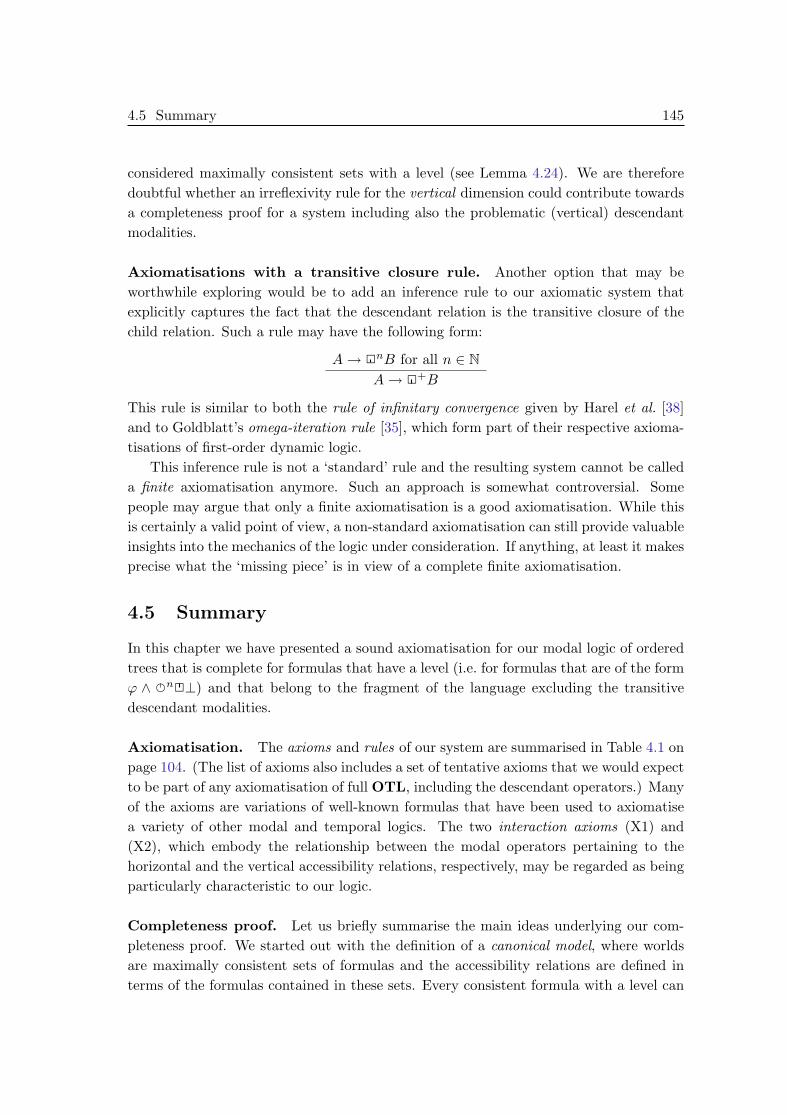
4.5 Summary 145
considered maximally consistent sets with a level (see Lemma 4.24). We are thereforedoubtful whether an irreflexivity rule for the vertical dimension could contribute towardsa completeness proof for a system including also the problematic (vertical) descendantmodalities.
Axiomatisations with a transitive closure rule. Another option that may beworthwhile exploring would be to add an inference rule to our axiomatic system thatexplicitly captures the fact that the descendant relation is the transitive closure of thechild relation. Such a rule may have the following form:
A→ 2nB for all n ∈ NA→ 2+B
This rule is similar to both the rule of infinitary convergence given by Harel et al. [38]and to Goldblatt’s omega-iteration rule [35], which form part of their respective axioma-tisations of first-order dynamic logic.
This inference rule is not a ‘standard’ rule and the resulting system cannot be calleda finite axiomatisation anymore. Such an approach is somewhat controversial. Somepeople may argue that only a finite axiomatisation is a good axiomatisation. While thisis certainly a valid point of view, a non-standard axiomatisation can still provide valuableinsights into the mechanics of the logic under consideration. If anything, at least it makesprecise what the ‘missing piece’ is in view of a complete finite axiomatisation.
4.5 Summary
In this chapter we have presented a sound axiomatisation for our modal logic of orderedtrees that is complete for formulas that have a level (i.e. for formulas that are of the formϕ ∧ en2⊥) and that belong to the fragment of the language excluding the transitivedescendant modalities.
Axiomatisation. The axioms and rules of our system are summarised in Table 4.1 onpage 104. (The list of axioms also includes a set of tentative axioms that we would expectto be part of any axiomatisation of full OTL, including the descendant operators.) Manyof the axioms are variations of well-known formulas that have been used to axiomatisea variety of other modal and temporal logics. The two interaction axioms (X1) and(X2), which embody the relationship between the modal operators pertaining to thehorizontal and the vertical accessibility relations, respectively, may be regarded as beingparticularly characteristic to our logic.
Completeness proof. Let us briefly summarise the main ideas underlying our com-pleteness proof. We started out with the definition of a canonical model, where worldsare maximally consistent sets of formulas and the accessibility relations are defined interms of the formulas contained in these sets. Every consistent formula with a level can

146 Chapter 4. Axiomatic Characterisation
be extended to a maximally consistent set with a level. To show that consistent formulasare satisfiable, we have used these maximally consistent sets to generate a submodel ofthe canonical model and have shown that it satisfies the formula in question. We havealso shown that the frame underlying such a generated submodel must be a loosely or-dered tree. By our results obtained in the previous chapter, satisfiability with respect toloosely ordered trees is equivalent to satisfiability with respect to ordered trees.
The restriction to formulas with a level has served two main purposes. Firstly, thevertical accessibility relation restricted to any submodel of the canonical model gener-ated by a maximally consistent set with a level could easily be shown to be irreflexive.Secondly, the concept of a maximally consistent set with a level allowed us to provethe Ancestor Existence Lemma, i.e. it allowed us to show that the transitive ancestormodalities work as intended within the model used to show completeness. A similarconstruction for the descendant modalities is not possible, which explains the restrictionof our result to the fragment of OTL excluding the operators 3+ and 2+.
Alternatives. Towards the end of the chapter, we have discussed a number of potentialalternatives to our axiomatisation as well as to the method chosen to prove complete-ness. The standard approach to proving completeness for logics that include an operatorpertaining to the transitive closure of the accessibility relation of another operator is towork with finite sets of formulas that are Fischer-Ladner closed, rather than building upan infinite canonical model. While we cannot conclusively exclude the possibility of suchan approach being successful also in the case of OTL, we have discussed some of thedifficulties that we have encountered.
An interesting alternative to our axiomatisation, which we have mentioned onlybriefly, would be a system that includes one or more irreflexivity rules to characterise theirreflexivity of accessibility relations directly. We would expect the completeness prooffor such a system to be simpler than ours, but we do not necessarily expect to solve theproblems regarding the transitive descendant modalities in this manner.

Chapter 5
Decidability
Our aim for this chapter is to show that the modal logic of ordered trees is a decidablelogic. We are going to prove decidability by showing how our logic can be embeddedinto another logic that is very expressive but still known to be decidable. This logic isthe monadic second-order theory of two successor functions.
In the first section of this chapter we are going to introduce this logic and quoteRabin’s famous decidability result. Following that, we are going to approach our decid-ability proof for ordered tree logics through the study of two special cases. To beginwith, we are going to show that OTL is decidable, if we restrict the class of admissibleframes to finite binary trees.1 Then we are going to prove that OTL restricted to theclass of all discretely ordered trees is also a decidable logic. Finally, we are going to provedecidability for the full logic.
5.1 Monadic Second-order Logic
The objective of this first section is to introduce monadic second-order logic over thetheory of n successor functions. Our exposition is not intended to be complete and isessentially guided by our needs for proving decidability of ordered tree logics in the latersections. For further information on monadic second-order theories we therefore refer toRabin [61] and Thomas [67].
Second-order theories. First-order logic (as opposed to propositional logic) allowsfor quantification over variables. On top of that, second-order logic also allows for quan-tification over predicates. In monadic second-order logic, only unary predicate symbolsare admitted and consequently, besides simple variables, quantification is restricted tothose unary predicates. Semantically, unary predicate symbols represent sets (of objectswith a certain property), so another way of characterising monadic second-order logicwould be to say that it allows for quantification over both simple variables and sets.
1The resulting logic has previously been studied (and, amongst other things, shown to be decidable)
by Blackburn and Meyer-Viol [9].
147
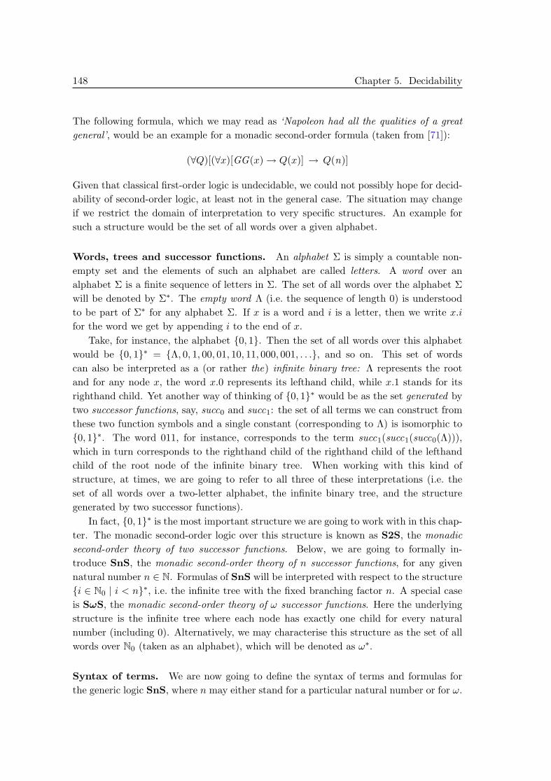
148 Chapter 5. Decidability
The following formula, which we may read as ‘Napoleon had all the qualities of a greatgeneral’, would be an example for a monadic second-order formula (taken from [71]):
(∀Q)[(∀x)[GG(x) → Q(x)] → Q(n)]
Given that classical first-order logic is undecidable, we could not possibly hope for decid-ability of second-order logic, at least not in the general case. The situation may changeif we restrict the domain of interpretation to very specific structures. An example forsuch a structure would be the set of all words over a given alphabet.
Words, trees and successor functions. An alphabet Σ is simply a countable non-empty set and the elements of such an alphabet are called letters. A word over analphabet Σ is a finite sequence of letters in Σ. The set of all words over the alphabet Σwill be denoted by Σ∗. The empty word Λ (i.e. the sequence of length 0) is understoodto be part of Σ∗ for any alphabet Σ. If x is a word and i is a letter, then we write x.ifor the word we get by appending i to the end of x.
Take, for instance, the alphabet 0, 1. Then the set of all words over this alphabetwould be 0, 1∗ = Λ, 0, 1, 00, 01, 10, 11, 000, 001, . . ., and so on. This set of wordscan also be interpreted as a (or rather the) infinite binary tree: Λ represents the rootand for any node x, the word x.0 represents its lefthand child, while x.1 stands for itsrighthand child. Yet another way of thinking of 0, 1∗ would be as the set generated bytwo successor functions, say, succ0 and succ1: the set of all terms we can construct fromthese two function symbols and a single constant (corresponding to Λ) is isomorphic to0, 1∗. The word 011, for instance, corresponds to the term succ1(succ1(succ0(Λ))),which in turn corresponds to the righthand child of the righthand child of the lefthandchild of the root node of the infinite binary tree. When working with this kind ofstructure, at times, we are going to refer to all three of these interpretations (i.e. theset of all words over a two-letter alphabet, the infinite binary tree, and the structuregenerated by two successor functions).
In fact, 0, 1∗ is the most important structure we are going to work with in this chap-ter. The monadic second-order logic over this structure is known as S2S, the monadicsecond-order theory of two successor functions. Below, we are going to formally in-troduce SnS, the monadic second-order theory of n successor functions, for any givennatural number n ∈ N. Formulas of SnS will be interpreted with respect to the structurei ∈ N0 | i < n∗, i.e. the infinite tree with the fixed branching factor n. A special caseis SωS, the monadic second-order theory of ω successor functions. Here the underlyingstructure is the infinite tree where each node has exactly one child for every naturalnumber (including 0). Alternatively, we may characterise this structure as the set of allwords over N0 (taken as an alphabet), which will be denoted as ω∗.
Syntax of terms. We are now going to define the syntax of terms and formulas forthe generic logic SnS, where n may either stand for a particular natural number or for ω.

5.1 Monadic Second-order Logic 149
We start with the definition of terms. The language for terms builds on a fixed countableset of variable names. To distinguish these variables from set variables, which we aregoing to introduce later on, we shall also refer to the former as simple variables.
Definition 5.1 (SnS terms) Let either n ∈ N or n = ω. We inductively define the setof terms in the language of the logic SnS as the smallest set such that:
(1) every (simple) variable is a term;
(2) if t is a term, so is succi(t) for all i ∈ N0 with i < n.
In the case of the logic SωS, condition (2) is supposed to express that there is a functionsymbol succi for every number i ∈ N0. Later on, we are mostly going to write x.i asa shorthand for succi(x); that is, we are going to use the same notation on both thesemantic and the syntactic level when describing the process of appending a single letterto the end of a given word.
Syntax of formulas. We now turn to the definition of the syntax of formulas for thegeneric logic SnS. Besides the set of simple variable names mentioned earlier we nowalso require a countable set of unary predicate symbols. We use capitals such as P andQ to denote predicate symbols and lowercase letters such as x and y for simple variablenames.
Definition 5.2 (SnS formulas) Let either n ∈ N or n = ω. We inductively define theset of well-formed formulas of the logic SnS as the smallest set such that:
(1) if P is a unary predicate symbol and t is an SnS term then P (t) is a formula;
(2) > and ⊥ are formulas;
(3) if ϕ and ψ are formulas, so are (¬ϕ), (ϕ ∧ ψ), (ϕ ∨ ψ), (ϕ→ ψ), and (ϕ↔ ψ);
(4) if x is a variable and ϕ is a formula, then (∃x)ϕ and (∀x)ϕ are also formulas;
(5) if P is a unary predicate symbol and ϕ is a formula, then (∃P )ϕ and (∀P )ϕ arealso formulas.
We shall also refer to unary predicate symbols as set variables, particularly so in contextswhere we quantify over a unary predicate symbol P , as in (∃P )ϕ. When writing formu-las, we are going to omit brackets whenever it is possible to do so without introducingambiguities.

150 Chapter 5. Decidability
Assignments. The structure over which we interpret formulas of a particular second-order theory is fixed. This will always be the appropriate structure of n successor func-tions. The only thing that can vary is the interpretation of particular variable namesand predicate symbols. This aspect of the semantics of SnS will be modelled by meansof so-called variable assignments.
Definition 5.3 (Assignments) An assignment α is a mapping from variable names towords and from set variable names to sets of words.
In the case of a logic SnS for some n ∈ N, an assignment α is understood to map simplevariable names to words over i ∈ N0 | i < n and unary predicate symbols to subsets ofi ∈ N0 | i < n∗. In the case of SωS, an assignment α will be a mapping to elementsand subsets of ω∗, respectively.
We will often say things such as ‘the set P contains the word x’ when in fact weshould be a little more formal and say that the word assigned to the variable x undersome assignment α belongs to the set of words assigned to the set variable P underassignment α. Occasionally, we are going to write xα rather than α(x) and Pα ratherthan α(P ) for simple variables x and set variables P , respectively.
Assignments extend from simple variables to terms in the obvious way. For everyi ∈ N0, the function symbol succi is interpreted as the function that appends the letteri at the end of a given word.
Definition 5.4 (Interpretation of terms) Let α be an SnS assignment. The defini-tion of α is inductively extended to SnS terms t as follows:
α(succi(t)) = α(t).i for i ∈ N0
The next definition provides us with a tool to speak about two assignments that onlydiffer in the interpretation of a single symbol (either a simple variable name or a predicatesymbol). This will be required later on to define the semantics of quantification.
Definition 5.5 (Assignment variants) Let α and α′ be assignments.
(1) Let x be a simple variable. Then α′ is called an x-variant of α iff α(y) = α′(y) forall variables y with y 6= x.
(2) Let P be a set variable. Then α′ is called an P -variant of α iff α(Q) = α′(Q) forall set variables Q with Q 6= P .
Truth with respect to an assignment. We are now ready to give a definition ofthe notion of truth for formulas of SnS. For each n there is just a single model, namelythe tree generated by n successor functions; so truth of a formula only depends on theassignment of its free variables to words and sets of words, respectively. We are going touse the same symbol (|=) to denote the truth relation as we have used for OTL. Indeed,

5.1 Monadic Second-order Logic 151
we are going to use the same symbol for all the various second-order logics, such as S2Sand SωS, we are going to work with in this chapter. Which logic we are referring to willalways be clear from the context, however.
Definition 5.6 (Truth of SnS formulas) We inductively define the notion of an SnSformula being true under an assignment α as follows:
(1) α |= P (t) iff α(t) ∈ α(P ) for unary predicate symbols P and terms t;
(2) α |= >;
(3) α |= ¬ϕ iff α 6|= ϕ;
(4) α |= ϕ ∧ ψ iff α |= ϕ and α |= ψ;
(5) α |= (∃x)ϕ iff α′ |= ϕ for some x-variant α′ of α;
(6) α |= (∃P )ϕ iff α′ |= ϕ for some P -variant α′ of α.
Observe that for closed formulas ϕ (i.e. for formulas without free variables of eitherkind) the assignment α does not matter. Such formulas will be either true under anyassignment or false under any assignment.
Definable operators. The operators not covered by Definition 5.6 are all definable interms of those for which we have provided a semantics.
Definition 5.7 (Definable SnS operators) The remaining operators of SnS are de-fined as abbreviations on the syntactic level:
ϕ ∨ ψ = ¬(¬ϕ ∧ ¬ψ) ⊥ = ¬>ϕ→ ψ = ¬ϕ ∨ ψ (∀x)ϕ = ¬(∃x)¬ϕϕ↔ ψ = (ϕ→ ψ) ∧ (ψ → ϕ) (∀P )ϕ = ¬(∃P )¬ϕ
The semantics of these operators can now be inferred from Definitions 5.6 and 5.7. It iseasily observed that, for any assignment α, we get:
(1) α 6|= ⊥;
(2) α |= ϕ ∨ ψ iff α |= ϕ or α |= ψ;
(3) α |= ϕ→ ψ iff α |= ϕ implies α |= ψ;
(4) α |= ϕ↔ ψ iff either both α |= ϕ and α |= ψ or neither;
(5) α |= (∀x)ϕ iff α′ |= ϕ for all x-variants α′ of α;
(6) α |= (∀P )ϕ iff α′ |= ϕ for all P -variants α′ of α.
152 Chapter 5. Decidability
Validity. Let us now define the concept of validity in the context of monadic second-order theories of n successor functions.
Definition 5.8 (Validity in SnS) An SnS formula ϕ is called valid iff α |= ϕ holdsfor every assignment α mapping variables into the structure of n successor functions.
If there exists at least one SnS assignment α such that α |= ϕ holds, then the formulaϕ is said to be satisfiable in the structure generated by n successor functions. Giventhat the assignment is irrelevant for formulas without free variables (of either kind), thenotions of validity and satisfiability coincide in the case of closed formulas.
As we shall see towards the end of this section, the validity problem for the monadicsecond-order theory of n successor functions may be reduced to that of the theory of twosuccessor functions, for any n ∈ N as well as for n = ω.
Decidability. The logic S2S was proved to be decidable by Rabin in 1969 [61]; thatis, there exists a procedure that, given a closed formula ϕ in the language of S2S, willdetermine, within a finite amount of time, whether or not ϕ is valid. This importantresult is known as Rabin’s Theorem:
Theorem 5.9 (Decidability of S2S) The monadic second-order theory of two succes-sor functions is decidable.
We are not going to prove this theorem here. The original proof is widely regarded asbeing particularly difficult. A more accessible proof may, for instance, be found in [67](see also references therein).
Our decidability proof for the modal logic of ordered trees (which we are going togive in Section 5.4), essentially, amounts to a reduction to this result.
Some definable predicates. In Rabin’s original formulation, the logic S2S also in-cludes two binary predicates, ≤ and ,2 with fixed semantics. For two variables x and y,the formula x ≤ y is intended to be true iff the word assigned to x is a (not necessarilyproper) prefix of the word assigned to y, while the formula x y holds iff the wordassigned to x precedes the word assigned to y in the lexicographic ordering declared over0, 1∗, or the two words are the same. Alternatively, as is well known, these predicatescan also be defined within the slightly slimmer incarnation of S2S we have introducedhere. In order to demonstrate some of the features of this logic, in what follows, we aregoing to show how to define these and a number of other useful predicates as abbrevia-tions on the syntactic level.
2Our use of the symbols ≤ and (and later on also < and ≺) in this chapter should not be confused
with the canonical accessibility relations from the previous chapter.

5.1 Monadic Second-order Logic 153
Equality. We start with a definition of a predicate to check whether two given termsare associated with the same word. This is a simple example where we use the second-order feature of S2S, i.e. quantification over sets of words (that is, over unary predicates).Observe that two objects are equal iff every set that contains the former also containsthe latter and vice versa. Hence, we can give the following definition of equality for twogiven terms t1 and t2:
(t1 = t2) = (∀P )[P (t1) ↔ P (t2)]
That is, we want the formula t1 = t2 to evaluate to true iff for every unary predicateP the formula P (t1) holds iff P (t2) does. This is the case precisely when t1 and t2 arebeing interpreted as the same word.
Subsets. Next we define a subset relation over set variables. This is easily expressiblein first-order logic alone:
(P ⊆ Q) = (∀x)[P (x) → Q(x)]
Given the subset relation, we can now also define the equality relation over sets:
(P = Q) = (P ⊆ Q) ∧ (Q ⊆ P )
Prefix ordering. Our next objective is to define the prefix relation ≤. We first givea formula that is true iff the set variable P appearing in that formula is interpreted asa set that is downward closed with respect to the prefix relation. That is, whenever aparticular word belongs to that set then every prefix of that word must belong to the setas well. For any given set variable P the formula prefix-closed(P ) defined as followsis true iff P is assigned to a prefix-closed set of words:
prefix-closed(P ) = (∀x)(∀y)[P (x) ∧ (y.0 = x ∨ y.1 = x) → P (y)]
Here, y stands for the immediate prefix of x (that is, we get from y to x by appendingeither a single 0 or a single 1). So the formula prefix-closed(P ) specifies that wheneverx belongs to P then so does x’s immediate prefix. Hence, by induction, every prefix ofx will be in P (possibly in addition to a number of other words, i.e. P is not necessarilythe smallest prefix-closed set for a particular word).
We can now define the (reflexive) prefix relation ≤ as follows:
(x ≤ y) = (∀P )[prefix-closed(P ) ∧ P (y) → P (x)]
The formula on the righthand side is true iff it is the case that every prefix-closed set Pthat contains y will also contain x. In particular, this will be the case for the smallestprefix-closed set P containing y, which contains only the prefixes of y and no other words.Hence, the word assigned to x will indeed be a prefix of the word associated with thevariable y.
Later on we are sometimes going to write x < y as an abbreviation for the properprefix relation (x ≤ y) ∧ ¬(x = y).

154 Chapter 5. Decidability
Identifying the root of the tree. A simple application of the prefix ordering ≤ isthe following definition of a predicate that allows us to identify the root of the infinitebinary tree, that is, the empty word Λ:
root(x) = (∀y)(x ≤ y)
The formula root(x) will be true under an assignment α iff α assigns the empty wordΛ to the variable x, because Λ is the only word that is a prefix of every word.
Lexicographic ordering. The next example shows that we can also treat the lexi-cographic ordering as a defined predicate. A word x precedes another word y in thelexicographic ordering declared over 0, 1∗ either if x is a prefix of y or x and y areidentical up to a certain letter and the next letter in x is 0 while there is a 1 at thecorresponding position in y. This notion is captured by the following definition:
(x y) = (x ≤ y) ∨ (∃z)[z.0 ≤ x ∧ z.1 ≤ y]
For example, the word 011010 lexicographically precedes 01110, because the two havethe common prefix 011 which is followed by a 0 in the former case and by a 1 in thelatter. Again, we are going to write x ≺ y as an abbreviation for (x y) ∧ ¬(x = y).
Finite sets. An interesting application of the lexicographic ordering is that we arenow in a position to write a formula that identifies a given set variable as referring toa finite set of words. Observe that induces a total order over the full set of words.We know that a totally ordered set must be finite iff each of its non-empty subsets hasboth a minimal and a maximal element with respect to the total order in question (seeProposition A.9 in Appendix A). This condition is expressible in second-order logic.
We first define abbreviations for formulas that express that the word assigned to agiven variable x is minimal (maximal) within the set assigned to some unary predicateQ with respect to the lexicographic ordering .
min(x,Q) = Q(x) ∧ (∀y)[Q(y) → x y]max(x,Q) = Q(x) ∧ (∀y)[Q(y) → y x]
Now we are in a position to give a formula that characterises a given unary predicate P asdenoting a finite set of words. The set assigned to P is finite iff for every set Q, wheneverQ is a subset of P that is not empty then there exists a word x that is minimal in Q andthere exists an(other) x that is maximal in Q with respect to the (total) lexicographicordering over words. Here is the corresponding formula:
finite(P ) = (∀Q)[Q ⊆ P ∧ (∃x)Q(x) → (∃x)min(x,Q) ∧ (∃x)max(x,Q)]
Having this ‘meta-predicate’ finite available to us, we can augment the language of S2Sto allow also for the quantification over finite sets of words. For instance, the formula

5.1 Monadic Second-order Logic 155
(∀Q)[finite(Q) → ϕ] is true iff ϕ is true whenever any free appearance of the variableQ within the formula ϕ is interpreted as a finite set. We introduce the following twoabbreviations:
(∃finQ)ϕ = (∃Q)[finite(Q) ∧ ϕ](∀finQ)ϕ = (∀Q)[finite(Q) → ϕ]
Guarded quantification. We are sometimes going to have to restrict quantificationover simple variables to words belonging to a particular set and quantification over setvariables to sets that are subsets of particular sets of words. To this end, we introducethe following shorthands for guarded quantification:
(∃x∈Q)ϕ = (∃x)[Q(x) ∧ ϕ] (∃P ⊆Q)ϕ = (∃P )[P ⊆ Q ∧ ϕ](∀x∈Q)ϕ = (∀x)[Q(x) → ϕ] (∀P ⊆Q)ϕ = (∀P )[P ⊆ Q→ ϕ]
Relations defined by formulas. It is important to keep in mind that our defined‘predicates’ such as root or ≤ are in fact nothing but syntactic abbreviations of certainS2S formulas. That is, even though, say, ≤ is (or has the appearance of being) abinary predicate, we are still working in the same monadic logic as before. Each definedpredicate that does not involve any free set variables determines a relation over thestructure generated by two successor functions. As we have seen earlier, the predicate≤, for example, determines the prefix relation over words in 0, 1∗. We are now goingto introduce notation that will allow us to speak about these relations directly.
Let pred(x1, . . . , xk) be an S2S formula with k free variables x1, . . . , xk (and no freeset variables). On the semantic level, this predicate corresponds to a k-ary relation overwords in 0, 1∗. This relation, which we are going to denote by JpredK, is defined asfollows:
JpredK = (w1, . . . , wk) ∈ (0, 1∗)k | α |= pred(x1, . . . , xk) for all αwith α(x1) = w1, . . . , α(xk) = wk
Here, α is understood to range over all S2S variable assignments. It follows from ourearlier discussion of the definition of the respective predicates that we have, for example,JrootK = Λ and J<K = (Λ, 0), (Λ, 1), (Λ, 00), (0, 00), (Λ, 01), (0, 01), . . ..
We are going to use the same kind of notation for the semantics of defined predicatesalso for SnS with n 6= 2 (simply substitute (0, 1∗)k by (i ∈ N0 | i < n∗)k or (ω∗)k,respectively, and let α range over variable assignments for the logic in question).
Encoding theories with more than two successor functions. We shall concludeour introduction to monadic second-order logic by showing how second-order theorieswith more than two successor functions, and particularly SωS, can be embedded intothe logic S2S. This is important, because it shows that, by Rabin’s Theorem, all of theselogics are decidable and we can pick the one that seems most convenient for our owndecidability proofs later on. We start with an encoding of SωS into S2S. The result forthe other logics will then follow by adding a simple additional restriction.

156 Chapter 5. Decidability
•Λ
• • • • • •
• • •• • • •
0
yyrrrrrrrrrrrrrrrrrrrrrrrrrrrr
%%
((
1 // 1 // 1 // 1 // 1 // //_____
0
1 // 1 // //____
0
##
1 // 1 // 1 // //____
Figure 5.1: Encoding SωS in S2S
The basic idea underlying this embedding is to use one of the two successor functionsof S2S to represent arbitrary natural numbers in a unary format and to use the otheras a separator between these unary numbers. For instance, the word 01111101111011(an element of 0, 1∗) may be interpreted as encoding the word 542 (an element of ω∗);0001111111 would stand for 007, and so on. If we think of 0, 1∗ as the infinite binarytree and of ω∗ as the infinite tree where every node has one child for every number inN0, then this observation shows that we can identify the latter as a kind of substructureof the former. Figure 5.1 shows how. To reach the nth child of a given node in the treeω∗, we first use succ0, the first successor function available in S2S, to go down to theleftmost child of a given node, and then succ1, the other S2S successor function, to moven steps to the right.
Formally, we can define a mapping f from ω∗ to 0, 1∗ as follows:
f(Λ) = Λf(x.i) = f(x).0.1i for i ∈ N0
This mapping is not surjective. In fact, inspection of the definition of f shows that weare mapping the set of words ω∗ onto the set of those words in 0, 1∗ that do not startwith a 1 (equivalently, we are mapping onto the set of words starting with 0 togetherwith the empty word Λ). This set of words can be characterised by an S2S formula:
fulltree(x) = ¬(∃y)[root(y) ∧ y.1 ≤ x]
The formula fulltree(x) will be satisfied under an assignment α iff α maps x to a wordthat does not start with a 1, i.e. a word that is in the range of the function f .
The language of SωS has one successor function for each natural number (including0). To distinguish the functions symbols of the two logics, we are going to write succω
i

5.1 Monadic Second-order Logic 157
with i ∈ N0 for successor functions of SωS and reserve the original symbols, namelysucc0 and succ1, for S2S. To be able to translate terms in the language of SωS intoterms in the language of S2S we have to show how to represent the function symbols ofSωS within S2S in a way that corresponds to the mapping f between the two infinitetrees. Here is a simple recursive definition of the translation function:
succω0 (x) = succ0(x)
succωi (x) = succ1(succω
i−1(x)) for i ∈ N
That is, the SωS term succω3 (x), for example, would be translated into the S2S term
succ1(succ1(succ1(succ0(x)))). In our shorthand notation, this means that x.3 would berepresented as x.0.1.1.1.
We are now in a position to describe the process of translating a (closed) SωS formulaϕ into an S2S formula ϕ∗ in such a way that ϕ is valid in SωS iff ϕ∗ is valid in S2S.The first step is to rewrite SωS terms as terms using only the two successor functions ofS2S. The next step is to ensure that variables in the translated formula only range overthose words (or set of words in the case of set variables) of 0, 1∗ that are in the rangeof the mapping f from 0, 1∗ to ω∗. To this end we introduce a special set variableT (which is different from any of the set variables used in ϕ) that is intended to beassigned to precisely that set of words. This assignment can be enforced by the formula(∀x)[fulltree(x) ↔ T (x)]. Furthermore, we replace every quantification in ϕ by aquantification guarded by T . That is, we rewrite (∃x) as (∃x∈T ) and ∃P as (∃P ⊆T ),and accordingly for universal quantifiers.
Let ϕT01 be the S2S formula we get by translating all function symbols in ϕ by the
appropriate combinations of succ0 and succ1 as well as replacing every quantificationwith a quantification guarded by the set variable T . Then the formula ϕ∗, defined asfollows, will be valid in S2S iff our original formula ϕ is valid in SωS:
ϕ∗ = (∀T )[(∀x)[fulltree(x) ↔ T (x)] → ϕT01]
Hence, by Rabin’s Theorem, SωS must be a decidable logic.
Example. Consider, for example, the SωS formula (∃P )(∀x)[P (x) → P (x.3)]. Thisformula is valid iff there exists a set of words that is closed under appending a 3 atthe end of a word. This is clearly the case; the infinite set Λ, 3, 33, 333, 3333, . . .,for instance, would be a candidate. To translate the formula we first have to fix aname, say T , for the set variable corresponding to the set of words in the range of thetranslation function f . Translating the formula itself then yields the following result:(∃P ⊆T )(∀x∈T )[P (x) → P (x.0.1.1.1)]. Before we can check validity we have to ensurethat T will be interpreted as intended, namely as the set of all words that correspond towords in ω∗. In summary, our original formula (∃P )(∀x)[P (x) → P (x.3)] is valid in thelogic SωS iff the following formula is valid in S2S:
(∀T )[(∀x)[fulltree(x) ↔ T (x)] → (∃P ⊆T )(∀x∈T )[P (x) → P (x.0.1.1.1)]]

158 Chapter 5. Decidability
Prefix and lexicographic ordering for SωS. The definitions of both the prefixand the lexicographic orderings over words given earlier in this sections were specificto S2S and analogous definitions for SωS are not possible, because we now have aninfinite number of successor functions to consider. However, it is possible to expressthese relations within the embedding of SωS into S2S just described.
Let a and b be two words in ω∗ and let f(a) and f(b) be their translations into 0, 1∗.If a is a proper prefix of b then this will manifest itself in the words f(a) and f(b) asfollows. The word f(b) will have f(a) as a prefix and that prefix will be followed by thetranslation of at least one more number, that is, the string f(a) will at least be followedby a 0 within the word f(b). The converse holds as well, that is, the formula x.0 ≤ y
characterises the proper prefix ordering for the embedding of SωS into S2S. We canthus use the formula (x.0 ≤ y) ∨ (x = y) to rewrite the usual (reflexive) prefix orderingof SωS when translating formulas into S2S.
Expressing the lexicographic ordering for SωS is even simpler. In fact, as is readilyverified, the lexicographic ordering of S2S acts also as a lexicographic ordering for SωS(if we use the embedding into S2S presented above). That is, no specific translation ofthe defined predicate is necessary.
Encoding theories with finitely many successor functions. The embedding ofSωS into S2S can easily be adapted in such a way as to serve as an embedding of SnSinto S2S for any finite n ∈ N. All that is required is an additional formula that furtherrestricts the substructure of 0, 1∗ used for the actual embedding to ensure that nosubstrings corresponding to numbers greater or equal to n can appear in the translationof an SnS word. To encode, for instance, the logic S4S we simply add the formula¬(∃y)(y.1.1.1.1 ≤ x) to the definition of the predicate fulltree(x).
It follows that SnS must be a decidable logic for any finite number of successorfunctions n ∈ N.
Defined predicates again. Observe that all the defined predicates discussed earlierare available in all our second-order logics. Whenever a definition does not make anyreference to successor functions at all (such as our definition of equality over words, forinstance), we can use the same formula for every logic. In cases where the successorfunctions are required (as in the definition of prefix-closed), the definition can easilybe adapted for logics SnS with a finite number n of successor functions.
However, this would not be possible in the case of SωS. Still, as we have seen earlier,the critical predicates, namely the prefix ordering ≤ and the lexicographic ordering forSωS can both be translated into formulas in S2S, the logic we have used to embed SωSinto. So indeed, all of the defined predicates we have seen in this section are availablein all of the second-order theories we have been discussing.
Applications in modal logic. It turns out that a variety of modal logics can be em-bedded into the monadic second-order theory of two successor functions. Given Rabin’s

5.2 Finite Binary Trees 159
Theorem, such an embedding would then show that the modal logic in question mustbe decidable. A number of early decidability results for modal logics using this methodwere obtained by Gabbay [27, 28].
We briefly outline some of the basic intuitions underlying this approach. For modallogics with a single fixed frame such as, for instance, the temporal logic over the rationalnumbers, the first crucial step for an embedding into S2S is a mapping from the set ofworlds in the modal frame to a suitable substructure of 0, 1∗ (similar to the mappingfrom ω∗ to 0, 1∗ discussed earlier). For modal logics defined with respect to a classof frames (rather than a single frame) we also have to show that we can capture anymember of this class by means of a set variable ranging over all possible sets of wordsthat could make up a frame of this logic. We also have to show that we can definepredicates that correspond to the accessibility relations of such frames. Finally, wehave to give a translation from modal formulas to second-order formulas. This will bevery similar to the standard translation of modal logic formulas into classical first-orderlogic and the translated formulas will directly refer to the predicates representing theaccessibility relations. Propositional letters of the modal language will be translated intounary predicates. We can use quantification over these predicates to simulate the rangeof all possible valuations.
Broadly speaking, this is the path we are going to follow for our decidability prooffor OTL. Of course, instead of embedding a modal logic directly into S2S, we may alsochoose to define an embedding into either SωS or SnS for some finite n ∈ N. Decidabilitythen follows from the fact that these second-order logics can themselves be embeddedinto S2S (as shown in this section).
Plan for the rest of this chapter. The following two sections may be consideredcase studies, where we use first S2S and then SωS to prove decidability for the va-lidity problem of OTL with respect to finite binary trees and discretely ordered trees,respectively. Our main decidability result, for OTL in general, will then be proved inSection 5.4 via a reduction to S4S.
5.2 Finite Binary Trees
In this section we are going to show how we can prove that the validity problem for OTLformulas with respect to finite binary trees is decidable via a reduction to Rabin’s The-orem. In fact, such a reduction is almost straightforward. Essentially, what is requiredare a translation from OTL formulas into S2S and a means of restricting reference fromthe infinite binary tree underlying S2S to arbitrary (finite) initial subtrees.
Modal logics of finite binary trees. In [9], Blackburn and Meyer-Viol introduce amodal logic of finite binary trees, demonstrate its relevance to applications in the area ofcomputational linguistics, prove completeness of a finite axiomatisation, and show that

160 Chapter 5. Decidability
their logic is decidable. Binary trees may be considered special cases of ordered trees. Ifevery internal node is known to have exactly two children, then we can always identifythe left and the right child of a node by reference to the order declared over siblings.Towards the end of the section on correspondences in Chapter 3, we have indicated howto express the modal operators available in the logic of Blackburn and Meyer-Viol interms of OTL operators, assuming that the class of admissible frames is restricted tobinary trees.
The following definition identifies the class of finite binary trees as a subclass of theclass of all ordered trees (as specified in Definition 3.4).
Definition 5.10 (Finite binary trees) An ordered tree T = (T,R, S) is called a finitebinary tree iff the set of nodes T is finite and the set of siblings [t]R−1R is a set withexactly two elements for every node t ∈ T except the root.
Defining the accessibility relations. The structure 0, 1∗ underlying the logic S2Sis a binary tree and thereby also an ordered tree. A first requirement for being ableto translate modal OTL formulas into S2S formulas is to show that the accessibilityrelations relevant to the semantics of OTL can be expressed in terms of S2S. Theseaccessibility relations are the descendant relation, the child relation, the sibling relation,the neighbour relation, and their inverses. Given that we are going to use the tree0, 1∗ itself, rather than using it to encode a differently structured tree first, expressingthese relations is easy. For instance, the descendant relation directly corresponds to the(proper) prefix relation introduced earlier:
descendant(x, y) = (x < y)
That is, the word represented by the variable x has as a descendant in the infinite binarytree 0, 1∗ the word represented by y iff the former is a proper prefix of the latter.The ancestor relation is the inverse of the descendant relation. That is, the formuladescendant(y, x) is true iff y represents an ancestor of the word represented by x inthe infinite binary tree. We could use the predicate descendant to define a predicatefor the child relation, namely by stipulating that y is the child of x iff y is a descendantof x and there is no other node that is both a descendant of x and an ancestor of y.Alternatively, we may also give a direct definition as follows:
child(x, y) = (x.0 = y) ∨ (x.1 = y)
This definition is based on the fact that if appending either a 0 or a 1 to the end of theword represented by x yields the word referred to by y then y represents the child of theword represented by x in the infinite binary tree. Again, we may also use the predicatechild to refer to the parent of a given node, because the two accessibility relations areinverse to each other. It follows from our definitions that the predicate descendant
must be interpreted as the transitive closure of the relation corresponding to the predicate

5.2 Finite Binary Trees 161
child, because the prefix relation is the transitive closure of the immediate prefix relationencoded by child.
Next we turn to the definition of an accessibility relation to refer to right- and lefthandsiblings. Two words represent sibling nodes iff they only differ in their final letter. Theword ending in 0 is the lefthand sibling; the one ending in 1 is the righthand sibling.That is, a sibling relation may be defined as follows:
sibling(x, y) = (∃z)(z.0 = x ∧ z.1 = y)
In the case of binary trees, the notions of sibling and neighbour coincide; thus:
neighbour(x, y) = sibling(x, y)
Characterising initial subtrees. The infinite binary tree generated by two successorfunctions is a particular ordered tree. The set of nodes is given by the set of words 0, 1∗.The child relation R of an ordered tree can be represented in terms of the child predicateand the sibling relation S corresponds to the sibling predicate. We would now be in aposition to prove decidability of the validity problem of OTL for the particular framegiven by the infinite binary tree. As we are interested in validity over the class of all(finite) binary trees, we first have to put forward suitable conditions that allow us todecide for any given subset of 0, 1∗ whether that set represents itself a binary tree ornot.
Observe that any given binary tree is isomorphic to an initial binary subtree of theinfinite binary tree. By an initial subtree we mean any subset of 0, 1∗ that includes theroot of the infinite tree (i.e. the empty word Λ) such that, whenever a node belongs tothis set, so does its parent. We furthermore call an initial subtree binary iff it containseither both or none of the two children of any given node. Using the defined predicatesencoding the accessibility relations together with the predicate root defined in theprevious section, we can express these properties as a formula with a free set variable Tcorresponding to the set of nodes that make up the respective initial binary subtree. Weabbreviate this formula as tree(T ):
tree(T ) = (∀x)[root(x) → T (x)] ∧(∀x)(∀y)[child(x, y) ∧ T (y) → T (x)] ∧(∀x)(∀y)[sibling(x, y) → (T (x) ↔ T (y))]
Now, if α is an S2S variable assignment such that α |= tree(T ) holds, then the triple(Tα, JchildK, JsiblingK) is a binary ordered tree.3 Also, for every binary tree there existsan assignment α such that (Tα, JchildK, JsiblingK) is isomorphic to that binary tree (forsome set variable T with α |= tree(T )). Furthermore, the relations induced on thesetrees by the predicates descendant and neighbour work as intended: JdescendantKis the transitive closure of JchildK and JneighbourK is the immediate successor relationunderlying JsiblingK.
3Of course, the relations JchildK and JsiblingK range over the entire infinite binary tree. If we wish
restrict them explicitly to Tα, we may write (Tα, JchildK ∩ Tα×Tα, JsiblingK ∩ Tα×Tα) instead.

162 Chapter 5. Decidability
The Translation Function trTx
trTx (P ) = P ′(x) for propositional letters P
trTx (>) = >
trTx (¬ϕ) = ¬trT
x (ϕ)trT
x (ϕ ∧ ψ) = trTx (ϕ) ∧ trT
x (ψ)trT
x ( eϕ) = (∃y∈T )[child(y, x) ∧ trTy (ϕ)]
trTx (3ϕ) = (∃y∈T )[descendant(y, x) ∧ trT
y (ϕ)]trT
x ( eϕ) = (∃y∈T )[neighbour(y, x) ∧ trTy (ϕ)]
trTx (3ϕ) = (∃y∈T )[sibling(y, x) ∧ trT
y (ϕ)]trT
x ( eϕ) = (∃y∈T )[neighbour(x, y) ∧ trTy (ϕ)]
trTx (3ϕ) = (∃y∈T )[sibling(x, y) ∧ trT
y (ϕ)]trT
x (3ϕ) = (∃y∈T )[child(x, y) ∧ trTy (ϕ)]
trTx (3+ϕ) = (∃y∈T )[descendant(x, y) ∧ trT
y (ϕ)]
P ′: set variable(s),encoding valuation forpropositional letter(s) P
T : set variable,encoding modal frame
x: simple variable,encoding world in frame
y: simple variable,fresh for each subformula
Table 5.1: Translating OTL formulas into monadic second-order logic
Translating modal formulas. We now turn to the actual translation of OTL formu-las into formulas of monadic second-order logic. This translation is going to be similarto the usual standard translation of modal logics into classical first-order logic.4 For thestandard translation, we require a binary first-order predicate for each of the accessibilityrelations referred to in the definition of the semantics of the respective modal logic. Here,this role will be filled by our previously defined predicates characterising the descendant,child, sibling, and neighbour relations in an ordered tree. As for the standard translation,every translated formula will have a single free variable x, which may be thought of asranging over the nodes in a tree. Furthermore, quantification in the translated formulaswill be guarded by a set variable T intended to represent the set of words used for theencoding of a particular ordered tree as a substructure of the infinite binary tree.
Our translation function trTx is defined in Table 5.1. The x in the subscript fixes
the name of the simple free variable in the resulting second-order formula and the Tis the name of the free set variable guarding quantification in the same formula. Anypropositional letter P appearing in an OTL formula ϕ to be translated will be representedby a unary predicate P ′ in the second-order formula trT
x (ϕ).
We are going to use the same translation function in the following two sections, wherewe are going to describe an encoding of discretely ordered trees into SωS and an encodingof general ordered trees into S4S, respectively. Only the definition of predicates, such asdescendant, encoding the accessibility relations is going to change, depending on theparticular construction.
4The standard translation for the basic modal logic has briefly been discussed in the introductory
Chapter 2. The standard translation from our logic OTL into classical first-order logic will also be
defined in Chapter 6.

5.3 Discretely Ordered Trees 163
Decidability for finite binary trees. We are now in a position to prove decidabilityof the validity problem for the modal logic of finite binary trees. To be able to phrasethis result as a specific decidability result for OTL we introduce the notion of OTLvalidity in finite binary trees.
Definition 5.11 (Validity in finite binary trees) A formula ϕ is called valid in fi-nite binary trees iff T |= ϕ holds for every finite binary tree T .
Our first Decidability Theorem now states that for any given OTL formula the problemof checking whether that formula is valid over the class of finite binary trees is a decidableproblem.
Theorem 5.12 (Decidability for finite binary trees) The problem of checking va-lidity in finite binary trees is decidable.
Proof. Let ϕ be an OTL formula and let P1, . . . , Pn be the propositional letters appearingin ϕ. Consider the S2S formula ϕ∗ defined as follows:
ϕ∗ = (∀finT )[tree(T ) → (∀P ′1⊆T ) · · · (∀P ′
n⊆T )(∀x∈T )trTx (ϕ)]
Here, trTx is the translation function given in Table 5.1 and the meta-predicate tree
as well as the binary predicates descendant, child, sibling, and neighbour (thelatter four of which feature in the definition of trT
x ) are understood to be the respectivepredicates as previously defined in this section.5 The predicates P ′
1, . . . , P′n are the unary
predicates we obtain when we translate the propositional letters P1, . . . , Pn.The formula ϕ∗ expresses that, for every finite subset of 0, 1∗ that is an initial
binary subtree of the infinite binary tree, we can choose the assignments to the predicatesymbols P ′
1 to P ′n so as to refer to any subsets of that finite tree, and the translation
of ϕ will be true on that particular structure. This is the case precisely iff ϕ is validwith respect to all finite binary trees. Hence, checking validity of ϕ (with respect tofinite binary trees) is equivalent to checking validity of ϕ∗ in S2S. By Rabin’s Theorem,the latter problem is decidable, so checking validity for finite binary trees must be adecidable problem as well. 2
Our discussion at the beginning of this section shows that Theorem 5.12 confirms oneof the results of Blackburn and Meyer-Viol [9], namely that their modal logic of finitebinary trees is decidable.
5.3 Discretely Ordered Trees
Our aim for this section is to improve on Theorem 5.12 and show that our logic remainsdecidable when we extend the class of frames under consideration from binary trees to
5In later sections, we are going to give different definitions for these four predicates.
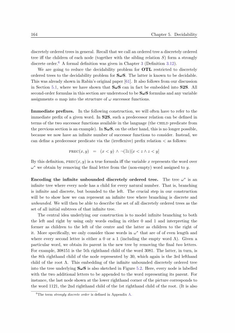
164 Chapter 5. Decidability
discretely ordered trees in general. Recall that we call an ordered tree a discretely orderedtree iff the children of each node (together with the sibling relation S) form a stronglydiscrete order.6 A formal definition was given in Chapter 3 (Definition 3.12).
We are going to reduce the decidability problem for OTL restricted to discretelyordered trees to the decidability problem for SωS. The latter is known to be decidable.This was already shown in Rabin’s original paper [61]. It also follows from our discussionin Section 5.1, where we have shown that SωS can in fact be embedded into S2S. Allsecond-order formulas in this section are understood to be SωS formulas and any variableassignments α map into the structure of ω successor functions.
Immediate prefixes. In the following construction, we will often have to refer to theimmediate prefix of a given word. In S2S, such a predecessor relation can be defined interms of the two successor functions available in the language (the child predicate fromthe previous section is an example). In SωS, on the other hand, this is no longer possible,because we now have an infinite number of successor functions to consider. Instead, wecan define a predecessor predicate via the (irreflexive) prefix relation < as follows:
prec(x, y) = (x < y) ∧ ¬(∃z)[x < z ∧ z < y]
By this definition, prec(x, y) is a true formula iff the variable x represents the word overω∗ we obtain by removing the final letter from the (non-empty) word assigned to y.
Encoding the infinite unbounded discretely ordered tree. The tree ω∗ is aninfinite tree where every node has a child for every natural number. That is, branchingis infinite and discrete, but bounded to the left. The crucial step in our constructionwill be to show how we can represent an infinite tree where branching is discrete andunbounded. We will then be able to describe the set of all discretely ordered trees as theset of all initial subtrees of that infinite tree.
The central idea underlying our construction is to model infinite branching to boththe left and right by using only words ending in either 0 and 1 and interpreting theformer as children to the left of the centre and the latter as children to the right ofit. More specifically, we only consider those words in ω∗ that are of of even length andwhere every second letter is either a 0 or a 1 (including the empty word Λ). Given aparticular word, we obtain its parent in the new tree by removing the final two letters.For example, 308151 is the 5th righthand child of the word 3081. The latter, in turn, isthe 8th righthand child of the node represented by 30, which again is the 3rd lefthandchild of the root Λ. This embedding of the infinite unbounded discretely ordered treeinto the tree underlying SωS is also sketched in Figure 5.2. Here, every node is labelledwith the two additional letters to be appended to the word representing its parent. Forinstance, the last node shown at the lower righthand corner of the picture corresponds tothe word 1121, the 2nd righthand child of the 1st righthand child of the root. (It is also
6The term strongly discrete order is defined in Appendix A.
5.3 Discretely Ordered Trees 165
•Λ
•01 •11 •21 •31•00•10•20•30
•01 •11 •21•00•10•20
***
****
****
*
???
????
????
????
?
%%LLLLLLLLLLLLLLLLLLLLLLL
((QQQQQQQQQQQQQQQQQQQQQQQQQQQQQQQQ
yyrrrrrrrrrrrrrrrrrrrrrrr
vvmmmmmmmmmmmmmmmmmmmmmmmmmmmmmmmm
((((((((((((
999
9999
9999
9999
##GGGGGGGGGGGGGGGGGGGG
wwwwwwwwwwwwwwwwwwww
Figure 5.2: Encoding the infinite unbounded discretely ordered tree in SωS
the righthand neighbour of the righthand neighbour of 1101, the ‘0th’ righthand child ofthe word 11.)
We now turn to the definition of the various SωS predicates required to describethe suggested embedding. The following two auxiliary predicates may be used to checkwhether a given variable x represents a word ending in 0 or 1, respectively:
left(x) = (∃y)(y.0 = x) right(x) = (∃y)(y.1 = x)
So left(x), for instance, will be true iff x represents a node that is one of the lefthandchildren of its parent (provided it represents one of the nodes used for the embedding inthe first place).
Every word in the set of words taken into account for our construction has to end ineither 0 or 1, or it has to be the empty word Λ. We can use the following meta-predicateto check whether a given set (assigned to a set variable P ) fulfils this condition:
zero-one(P ) = (∀x)[P (x) → root(x) ∨ left(x) ∨ right(x)]
Another requirement for the subset of ω∗ representing the unbounded infinite tree isthat it contains the empty word Λ. We can reuse the predicate root to specify a meta-predicate for set variables P that evaluates to true iff the corresponding set contains theempty word:
rooted(P ) = (∃x)[root(x) ∧ P (x)]
Another property of the set of words used to encode the unbounded tree is that, wheneverthat set contains a given word, it will also contain the predecessor of the predecessor ofthat word. In other words, the set is closed under removing the last two letters of aword. This property of a set is captured by our next meta-predicate:
gap-closed(P ) = (∀x)(∀y)(∀z)[prec(x, y) ∧ prec(y, z) ∧ P (z) → P (x)]

166 Chapter 5. Decidability
We are now going to put together the various auxiliary predicates defined earlier andpresent a predicate that defines the set of words in ω∗ that are used for our encoding ofthe unbounded discretely ordered tree indicated in Figure 5.2. How can we characterisethe set of words that make up this substructure of ω∗? Suppose we take a single wordx and use it to generate a set of words P as follows: x is in P and for any word in P
also the word we get by removing the last two letters is in P (provided that word hasat least two letters). This latter operation can be implemented by means of our definedpredicate gap-closed. Then the generated set P shows whether or not x is one of thewords we are looking for. If it is, then every word in P has to end either in a 0 or a 1(this can be implemented using zero-one) and the empty word Λ has to be part of P(that is, P has to be rooted). The latter guarantees that the original word x must havebeen of even length. In summary, the following predicate fulltree determines the setof words required for our construction:
fulltree(x) = (∀P )[P (x) ∧ gap-closed(P ) → rooted(P ) ∧ zero-one(P )]
The universal quantification over P guarantees that rooted(P ) ∧ zero-one(P ) holds,in particular, for the smallest set P that satisfies P (x) ∧ gap-closed(P ).
Defining the accessibility relations. If both x and y represent words that belongto the full tree then the latter is a descendant of the former iff it is one of its prefixes. Inother words, the prefix relation of ω∗ restricted to the set of words used to represent theunbounded discretely ordered tree coincides with the descendant relation declared overthe latter. Hence, the following is a suitable definition of the descendant predicate forthis construction:
descendant(x, y) = (x < y)
We have again more than one option of how to define the child relation. One of themwould be to exploit the fact that we get from a given word to the word representingits parent by removing the last two letters, that is, the parent of a node is representedby the immediate prefix of the immediate prefix of the word representing the node inquestion. Here is the corresponding definition of our new child predicate:
child(x, y) = (∃z)[prec(x, z) ∧ prec(z, y)]
Defining a suitable sibling predicate now is a little more involved than in the previoussection. Certainly, two nodes are siblings whenever they share a common parent. Thisobservation will enter our definition of the new sibling predicate, but it is not enoughto determine which of the two nodes lies to the left of the other. Suppose we havealready established that two given variables x and y represent sibling nodes in the infiniteunbounded tree. We can then distinguish three cases in which x would correspond to anode somewhere to the left of the node represented by the variable y:
(1) First, assume both x and y are lefthand children of their common parent (i.e. bothof them end in 0). Let z stand for the parent. Then x is of the form z.i.0 and y is

5.3 Discretely Ordered Trees 167
of the form z.j.0 (for some i, j ∈ N0). The word z.i.0 represents a node somewhereto the left of z.j.0 iff i is a greater number than j. This is the same as to saythat y lexicographically precedes x. Hence, if both x and y are lefthand childrenof their common parent then x is a lefthand sibling of y iff y strictly precedes x inthe lexicographic order ≺ declared over ω∗.
(2) By an analogous argument, if both x and y are righthand children of their commonparent then x is a lefthand sibling of y iff x ≺ y.
(3) Finally, x is also a lefthand sibling of y iff x ends in 0 and y ends in 1.
If none of these three conditions applies, then x cannot be a lefthand sibling of y. Alto-gether, we end up with the following definition of sibling:
sibling(x, y) = (∃z)[child(z, x) ∧ child(z, y)] ∧[(left(x) ∧ left(y) ∧ y ≺ x) ∨(right(x) ∧ right(y) ∧ x ≺ y) ∨(left(x) ∧ right(y))]
Finally, we define a neighbour relation over the infinite unbounded discretely orderedtree by stipulating that two nodes x and y are neighbours iff they are siblings and thereexists no other node z that is both a righthand sibling of x and a lefthand sibling of y:
neighbour(x, y) = sibling(x, y) ∧ ¬(∃z)[sibling(x, z) ∧ sibling(z, y)]
Before we can accept the above definition of the neighbour predicate, however, wehave to make the following observation. The set of words used to encode a particulardiscretely ordered tree will be a proper subset of ω∗. The variable z featuring in thedefinition above is intended to represent nodes in this substructure only. That is, ourcharacterisation of particular ordered trees later on will have to be such that, whenevertwo nodes are supposed to represent neighbours, then there can be no other word in ω∗
that would be a righthand sibling of the first node and a lefthand sibling of the secondif it was itself part of the chosen ordered tree. (Another option would have been toexplicitly guard the quantification over z.)
Characterising initial subtrees. Just as every strongly discrete order is isomorphicto a suborder of the integers, every discretely ordered tree is isomorphic to an initialsubtree of the infinite unbounded discretely ordered tree we have embedded into ω∗. Infact, it even suffices to only consider certain subtrees which we shall call initial subtreeswithout gaps. These are initial subtrees satisfying the following two properties:
(1) Whenever a word x ending in 0 belongs to the subtree, so do any of the righthandsiblings of x which themselves end in 0.
(2) Similarly, whenever a word ending in 1 belongs to the subtree, so do any of itslefthand siblings which themselves end in 1.

168 Chapter 5. Decidability
This class of trees allows us to represent any finite branching factor as well as infinitebranching that is either bounded to the left, bounded to the right, or unbounded ineither direction. This covers all cases, just as there are only three distinct infinite ordertypes that are strongly discrete: the positive integers (bounded to the left), the negativeintegers (bounded to the right), and the whole set of the integers (unbounded).
The following meta-predicate encodes the class of initial subtrees without gaps. Theconditions are similar to the definition of tree(T ) in the previous section. In additionto that, we also have to ensure that T represents a subset of the words satisfying ourdefined predicate fulltree and that there are no gaps between sibling nodes.
tree(T ) = (∀x)[T (x) → fulltree(x)] ∧(∀x)[root(x) → T (x)] ∧(∀x)(∀y)[child(x, y) ∧ T (y) → T (x)] ∧(∀x)(∀y)[sibling(x, y) ∧ left(y) ∧ T (x) → T (y)] ∧(∀x)(∀y)[sibling(x, y) ∧ right(x) ∧ T (y) → T (x)]
Let α be an SωS variable assignment mapping the set variable T to a subset of ω∗. Ourdiscussion shows that (Tα, JchildK, JsiblingK) will be a discretely ordered tree wheneverα |= tree(T ) holds. Also, vice versa, for any discretely ordered tree there exists anassignment α such that this tree is isomorphic to (Tα, JchildK, JsiblingK) for some setvariable T with α |= tree(T ). Furthermore, restricted to any Tα with α |= tree(T ),the relation JdescendantK is the transitive closure of JchildK and JneighbourK is theimmediate successor relation underlying JsiblingK.
Decidability for discretely ordered trees. Before we state the decidability resultfor this section, we give a formal definition of the class of formulas that are valid withrespect to discretely ordered trees.
Definition 5.13 (Validity in discretely ordered trees) A formula ϕ is called validin discretely ordered trees iff T |= ϕ holds for every discretely ordered tree T .
Here is our Decidability Theorem for discretely ordered trees:
Theorem 5.14 (Decidability for discretely ordered trees) The problem of check-ing validity in discretely ordered trees is decidable.
Proof. Let ϕ be an OTL formula and let P1, . . . , Pn be the propositional letters thatappear in it. Now consider the SωS formula ϕ∗ defined as follows:
ϕ∗ = (∀T )[tree(T ) → (∀P ′1⊆T ) · · · (∀P ′
n⊆T )(∀x∈T )trTx (ϕ)]
trTx is again the translation function given in Table 5.1, but this time the predicates
descendant, child, sibling, and neighbour used in the definition of trTx are the

5.4 General Ordered Trees 169
respective SωS predicates defined in this section. The meta-predicate tree is our pred-icate encoding initial subtrees without gaps. The set variables P ′
1, . . . , P′n are the unary
predicates we obtain when translating the propositional letters P1, . . . , Pn.The formula ϕ∗ says that for any initial subtree without gaps (represented by T ) of
the unbounded discretely ordered tree (which we have encoded as a substructure of ω∗)and for any sets of words (that is, any subsets of the set of words assigned to T ) assignedto the set variables P ′
1 to P ′n, the translation of the formula ϕ will be true, whatever
node of the subtree we assign the variable x to. This is the case iff ϕ is valid withrespect to any discretely ordered tree. Hence, checking validity of ϕ in discretely orderedtrees is equivalent to checking validity of ϕ∗ in SωS. The latter problem is known to bedecidable, i.e. checking validity for discretely ordered trees must be a decidable problemas well. 2
5.4 General Ordered Trees
In this section, we are going to show that OTL is a decidable logic. The proof falls intotwo parts. We first show how OTL with (almost) no restrictions on the admissible classof frames can be embedded into S4S (and thereby into S2S). The only restriction thatwe cannot eliminate is that for any such embedding the set of nodes in the respectiveordered tree will have to be countable.7 Therefore, in the second part of our proof wehave to show that, in fact, this restriction does not matter: any satisfiable formula willalso be satisfiable in a model based on an ordered tree with a countable set of nodes.
As for the first part of our proof, the crucial step up from Theorem 5.14 is that weare now going to drop the restriction to discretely ordered trees. In particular, generalordered trees allow for sibling nodes that are densely ordered. Therefore, before wedescribe the main construction of an infinite densely ordered tree, we are going to showhow we can encode a single dense order into S2S.
Encoding dense orders in S2S. Our construction follows that given by Gabbay etal. [30]. The basic idea is to ‘project’ the nodes of the infinite binary tree underlyingS2S down onto a straight line as shown in Figure 5.3.
Intuitively, such a projection induces a left-to-right ordering on the set of words in0, 1∗. Given a word x, the word x.0 is supposed to lie slightly to the left of x, whilethe word x.1 lies a little to its right. However, neither of them will lie as far to the leftor right of x as any of the prefixes (or ancestors) of x. In other words, x.1 for instance,will lie half way between x and the longest prefix of x ending in 1 (if any), i.e. the closestancestor of x (with respect to the binary tree) lying itself to the righthand side of x. We
7In the literature, sets that are either finite or countably infinite are sometimes called at most countable.
Here, we do not always make this distinction and simply refer to both finite and countably infinite sets
as countable ones.

170 Chapter 5. Decidability
•Λ
•0
•0
•0 •1
•1
•0 •1
•1
•0
•0 •1
•1
•0 •1
000 00 001 0 010 01 011 Λ 100 10 101 1 110 11 111
???
????
???
???
?
?
???
???
????
????
????
????
????
???
????
???
???
?
?
???
oo //
Figure 5.3: Encoding dense orders in S2S
now formally define this left-to-right ordering as follows:8
x y = x.1 ≤ y ∨ y.0 ≤ x ∨ (∃z)[z.0 ≤ x ∧ z.1 ≤ y]
That is, we have x y iff x 6= y and there is a node w in the tree such that x is either witself, its lefthand child, or a descendant of its lefthand child, and y is either w itself, itsrighthand child, or a descendant of its righthand child. The first disjunct describes thecase where x is that dominating node w and y is either its righthand child or a descendantof the latter. The second disjunct describes the case where y is the dominating node wand x is either its lefthand child or a descendant of the latter. The third disjunct, finally,describes the case where both x and y are descendants of a common ancestor w; x iseither its lefthand child or a descendant of its lefthand child and y is either its righthandchild or a descendant of its righthand child.
We are now going to show that the definition of the predicate really yields thekind of left-to-right ordering we intended: it induces a strict linear order over the set ofall words 0, 1∗ that is dense and without endpoints. We also remark that this ordermust be countable, the significance of which we are going to comment on at a later pointin this section. To establish that (0, 1∗,) is a strict linear order we have to checkthat it is indeed irreflexive, transitive, and connected:
(1) Irreflexivity. Follows immediately from the definition of .8The binary predicate induces a binary relation JK over the set of words 0, 1∗. However, to
simplify notation, in the sequel we are not always going to make this distinction and shall usually use
the symbol also for the (semantic) relation.

5.4 General Ordered Trees 171
(2) Transitivity. Again, this follows directly from the definition of (see also theexplanation given just after the definition).
(3) Connectedness. Any two words in 0, 1∗ that are not identical must either havea common proper prefix (possibly Λ) or one must be a proper prefix of the other.Hence, we have x = y or x y or y x for any two words x, y ∈ 0, 1∗, that is,the relation induced by must be connected.
Next we show that the linear order (0, 1∗,) must be dense, i.e. for any x, y ∈ 0, 1∗
with x y there exists a word z ∈ 0, 1∗ such that x z and z y. According to thedefinition of , we can distinguish three cases. Firstly, if x y holds because x.1 ≤ y
does, then the word y.0 fulfils our requirements: we have x y.0 y. Secondly, if wehave x y by virtue of y.0 ≤ x then x.1 does the job, i.e. we get x x.1 y. Andthirdly, in case we have x y because of (∃z)[z.0 ≤ x ∧ z.1 ≤ y] then that word z issuch that x z y holds. Hence, (0, 1∗,) is indeed dense.
Next we observe that for any word x there exist both words that precede and wordsthat succeed x in the order induced by , i.e. (0, 1∗,) is an order without endpoints.For instance, we have x.0 x and x x.1 for any word x ∈ 0, 1∗.
Finally, 0, 1∗ must be a countable set, because there is a direct bijective mappingbetween 0, 1∗ and the natural numbers in their binary representation (simply add asingle 1 at the beginning of each word).
A quick remark on the side, before we move on and use this kind of constructionfor our own purposes: By Cantor’s Theorem [12], any two countable dense linear orderswithout endpoints are isomorphic to each other. In particular the theory of the rationalnumbers (Q, <) will be isomorphic to (0, 1∗,). Hence, an immediate consequence ofthe above construction would be that the monadic second-order theory of (Q, <) — aswell as that of any other countable unbounded dense linear order — is decidable [30, 61].This result can serve as a basis for proving decidability results for linear temporal logicover various flows of time. We refer to Gabbay et al. [30] for more information on thissubject.
Encoding the infinite densely ordered tree. As we have already mentioned at thebeginning of this section, our first step in proving decidability for the full logic OTL willbe to construct an infinite tree where the children of each node form a (countable) denselinear order without endpoints. We have just seen how to encode a single dense orderinto S2S, but this involved collapsing the entire binary tree. How are we going to getback to a tree while maintaining density at the same time?
The basic ideas underlying our construction are illustrated in Figure 5.4. Ratherthan using S2S we are now going to use S4S, the monadic second-order theory of foursuccessor functions. For the set of children of any given node in the infinite denselyordered tree we are going to use either the first two successor functions succ0 and succ1
or the second two successor functions succ2 and succ3 to encode a countable dense linearorder without endpoints in the same way as we have just seen. In addition, by alternating

172 Chapter 5. Decidability
Λ
•0
•0
•0 •1 •0 •1
1 •0
•0 •1 0 •1
•1
•1
01
•2
•2
•2 •3 2 •3
•3 •2
•2 •3 •2 •3
3
•3
110
2/3
01232
0/1
0133
0/1
???
????
??
??
???
????
????
????
??
???
????
??
??
______________ ______________
_ _ _ _ _ _ _ _ _ _ _ _ _ _ _ _ _ _ _ _ _ _ _ _ _ _ _ _
???
????
??
??
???
????
????
????
??
???
????
??
??
______________ ______________
_ _ _ _ _ _ _ _ _ _ _ _ _ _ _ _ _ _ _ _ _ _ _ _ _ _ _ _
????
????
?____ ____
_ _ _ _ _ _ _ _ _
????
????
?____ ____
_ _ _ _ _ _ _ _ _
????
????
?____ ____
_ _ _ _ _ _ _ _ _
Figure 5.4: Encoding the infinite (densely) ordered tree in S4S
between the two pairs of successor functions, we can simulate the levels in a tree. Forinstance, the word 01 represents an element in the dense linear order we can map theset of words 0, 1∗ to. Similarly, the word 232 represents an element in the dense linearorder we can embed into 2, 3∗ in precisely the same way. Now the concatenation ofthe two, i.e. the word 01232, may be considered representing a node on the second levelof the infinite ordered tree. Nodes on the third level are again encoded using the firsttwo successor functions, and so on.
The empty word Λ is used to represent the root of the ordered tree, that is, it isnot part of the dense linear order of nodes from the first level below the root. Similarly,appending Λ (now considered an element of 2, 3∗) to the end of, say, 01 yields again01, i.e. we stay on the first level of nodes. Of course, removing a single element (namely

5.4 General Ordered Trees 173
Λ) from a countable dense linear order without endpoints yields again a countable denselinear order without endpoints, and the two are isomorphic to each other. Hence, ourconstruction really does result in an infinite ordered tree where the set of children of anygiven node form a countable dense linear order without endpoints which is, for instance,isomorphic to the order of the rationals (Q, <).
Our suggested embedding of the infinite densely ordered tree into S4S makes use ofall the words in 0, 1, 2, 3∗, except those that begin with either a 2 or a 3. This set ofwords is characterised by the following predicate:
fulltree(x) = ¬(∃y)[root(y) ∧ (y.2 ≤ x ∨ y.3 ≤ x)]
Defining the accessibility relations. We now turn to the definition of the crucialaccessibility relations over the infinite densely ordered tree for our embedding. Thedescendant predicate to be defined will have a lot in common with the strict prefixrelation < declared over words in 0, 1, 2, 3∗: in ‘most’ cases, if x is a proper prefix ofy, then the former will in fact represent an ancestor of the latter in the embedded tree.However, this is not the case if a node and its prefix encode elements of the same denselinear order. That is, to find out whether x represents an ancestor of y, we have to checknot only that x is a proper prefix of y, but also that, when we ‘move’ from the encodingof x to that of y, at least one change in the pair of successor functions used will takeplace. For instance, if x ends either in 0 or in 1, then the prefix identical to x within y
has to be immediately followed by either a 2 or a 3. A special case is the empty wordΛ, which represents the root of the embedded tree and thereby an ancestor of any othernode. Here is the formal definition of the descendant predicate for this embedding:
descendant(x, y) = [(∃z)(z.0 = x ∨ z.1 = x) ∧ (x.2 ≤ y ∨ x.3 ≤ y)] ∨[(∃z)(z.2 = x ∨ z.3 = x) ∧ (x.0 ≤ y ∨ x.1 ≤ y)] ∨[root(x) ∧ ¬root(y)]
A predicate for the child relation in the infinite ordered tree can be expressed in termsof the descendant predicate as follows:
child(x, y) = descendant(x, y) ∧ ¬(∃z)[descendant(x, z) ∧ descendant(z, y)]
We should point out that whenever x and y are mapped to words that are being usedfor the embedding of the infinite ordered tree (i.e. if both of them are mapped to wordsnot starting with either 2 or 3), then any word assigned to z validating the formuladescendant(x, z) ∧ descendant(z, y) would also have to belong to that set of wordsused for the embedding. Hence, no explicit restriction of the quantification over z in theabove definition of the child predicate is necessary.
Our new definition of the sibling predicate is similar to that of the predicate ,which we have seen earlier as part of the encoding of a dense linear order into S2S.We first use the child predicate to check that two given variables x and y do representsibling nodes at all. If they do, then either both of them will end in 0 or 1 or both of

174 Chapter 5. Decidability
them will end in 2 or 3. In the former case, we simply copy the definition of givenearlier; in the latter case we rewrite any 0 as a 2 and any 1 as a 3. We thus end up withthe following definition:
sibling(x, y) = (∃z)[child(z, x) ∧ child(z, y)] ∧[(x.1 ≤ y ∨ y.0 ≤ x ∨ (∃z)(z.0 ≤ x ∧ z.1 ≤ y)) ∨(x.3 ≤ y ∨ y.2 ≤ x ∨ (∃z)(z.2 ≤ x ∧ z.3 ≤ y))]
As for the embedding discussed in the previous section, we can again express theneighbour predicate in terms of the sibling predicate just defined. An importantdifference is that, this time, we are going to consider all initial subtrees of the infinitedensely ordered trees, which means that we have to be more careful regarding the quan-tification over words that may represent sibling nodes in between the two nodes checkedfor neighbourhood. We solve this problem by explicitly restricting the quantification overthe variable z in the following definition of neighbour by the set variable T , which isgoing to represent the set of nodes making up the initial subtree in question later on:
neighbour(x, y) = sibling(x, y) ∧ ¬(∃z ∈ T )[sibling(x, z) ∧ sibling(z, y)]
Strictly speaking, the neighbour predicate takes three arguments: the two variablesx and y, and the set variable T . However, as the symbol T will stay fixed for all usesof this predicate, we have not explicitly referred to it on the lefthand side of the abovedefinition.
Characterising initial subtrees. The last part of our construction concerns againthe characterisation of the set of all initial subtree of the infinite ordered tree, in orderto capture the class of all countable ordered trees. This time, we take all possible initialsubtrees into account, i.e. the definition of our new tree is straightforward. We have toensure that the set variable T is interpreted as a subset of the set of words characterisedby the fulltree predicate, that the empty word Λ is part of that set, and that for anyword belonging to the set also the word representing its parent node is included.
tree(T ) = (∀x)[T (x) → fulltree(x)] ∧(∀x)[root(x) → T (x)] ∧(∀x)(∀y)[child(x, y) ∧ T (y) → T (x)]
Just as any (at most) countable linear order is isomorphic to a substructure of a countabledense linear order without endpoints, any ordered tree with a set of nodes that is (atmost) countable will be isomorphic to an initial subtree of the infinite densely ordered treecharacterised by the defined predicate fulltree, together with the accessibility relationsJchildK and JsiblingK. That is, if α is an assignment for S4S mapping the set variableT to a subset of 0, 1, 2, 3∗ such that α |= tree(T ) holds, then (Tα, JchildK, JsiblingK)will be a countable ordered tree. As for the other direction, every ordered tree witha countable set of nodes is isomorphic to (Tα, JchildK, JsiblingK) for some variableassignment α.

5.4 General Ordered Trees 175
Furthermore, by construction, JdescendantK will be the transitive closure of JchildKand JneighbourK will the immediate successor relation induced by JsiblingK.
Decidability for countable ordered trees. We are now in a position to prove thatour logic OTL, restricted to ordered trees with countable sets of nodes, is decidable.Let us first capture the notion of validity with respect to this class of frames in a formaldefinition:
Definition 5.15 (Validity in countable ordered trees) A formula ϕ is called validin countable ordered trees iff T |= ϕ for all ordered trees T = (T,R, S) such that T is aset that is at most countable.
Here is our intermediate decidability result:
Lemma 5.16 (Decidability for countable ordered trees) The problem of checkingvalidity in countable ordered trees is decidable.
Proof. Let ϕ be an OTL formula and let P1, . . . , Pn be the propositional letters appearingin ϕ. We define the S4S formula ϕ∗ as follows:
ϕ∗ = (∀T )[tree(T ) → (∀P ′1⊆T ) · · · (∀P ′
n⊆T )(∀x∈T )trTx (ϕ)]
Here, trTx is the translation function defined in Table 5.1. The predicates descendant,
child, sibling, and neighbour referred to in the definition of trTx are understood to
be the respective S4S predicates defined earlier in this section. In particular, the unarypredicate symbol T appearing as a parameter of the translation function trT
x is the samesymbol as that appearing in the definition of the neighbour predicate. The set variablesP ′
1, . . . , P′n correspond to the propositional letters P1, . . . , Pn.
The formula ϕ∗ expresses that for any initial subtree (represented by the set variableT ) of the countably infinite densely ordered tree and any possible assignments of subsetsof the set of words assigned to T to the set variables P ′
1, . . . , P′n, as well as any possible
assignment of an element of that same set to the variable x, the translation of ϕ willbe true. This is precisely the case iff the formula ϕ is valid in countable ordered trees.Hence, the problems of checking validity of ϕ in countable ordered trees and checkingvalidity of ϕ∗ in S4S are in fact equivalent. Given that the latter is known to bedecidable, we find that checking validity with respect to countable ordered trees mustbe decidable as well. 2
Lemma 5.16 strongly suggests that OTL is decidable, also without the restriction tocountable frames. In the remainder of this section we are going to verify this intuitionand prove that the concepts of validity, on the one hand, and validity with respect tocountable ordered trees, on the other, do in fact coincide.

176 Chapter 5. Decidability
Eliminating the restriction to countable ordered trees. We say that a formula ϕhas got a countable ordered tree model iff there is an ordered tree model M = (T,R, S, V )such that T is an (at most) countable set and M, t |= ϕ holds for some node t ∈ T . Thefollowing lemma states that every formula that has got an ordered tree model will alsohave a countable ordered tree model (the converse trivially holds as well).
The corresponding result in classical first-order logic is known as the downwardLowenheim-Skolem Theorem: every first-order sentence with a model has got a count-able model [14]. We also have similar results in linear temporal logics: the language oftemporal logic cannot ‘distinguish’ countable models from those that are not countable.One way of proving this kind of result would be to translate into first-order logic andthen to appeal to the downward Lowenheim-Skolem Theorem [30]. This kind of approachseems likely to also be applicable in the case of OTL. Nevertheless, we choose to proveour lemma via a direct argument here.
Lemma 5.17 (Countable models) Every formula with an ordered tree model has gota countable ordered tree model.
Proof. Let ϕ be a satisfiable formula. We are going to show how we can transform a given(possibly uncountable) model for ϕ into a countable model. Recall that the depth of anordered tree is always countable. Hence, it is enough to reduce the tree underlying theoriginal model to a tree where every internal node has got a countable set of children; theoverall number of nodes will then be countable as well. In fact, we are going to transformthe original model of ϕ into a general model based on a loosely ordered tree (withoutcycles) where every set of pseudo siblings is countable.9 It follows from our constructionin the proof of Lemma 3.39 in Chapter 3 that the corresponding ordered tree will haveat most countably many children for every node (because we have bulldozed using onlyintegers and rationals, either of which are countable).
A formula ϕ is satisfiable iff there is a model based on an ordered tree where ϕ∨3+ϕ
is satisfied at the root. Hence, without loss of generality, we may assume that our inputformula ϕ is true at the root of the ordered tree of the original model.
Types. Before we turn to the description of the transformation of the original modelinto a model based on a countable loosely ordered tree, we introduce the notion of atype of a node. Let ϕ be our satisfiable input formula and let M = (T,R, S, V ) be theoriginal ordered tree model satisfying ϕ at the root. Furthermore, let sf (ϕ) denote theset of subformulas of ϕ (including ϕ itself).
We define the type of a node t ∈ T as the set of subformulas of ϕ satisfied at t inthe original model, i.e. as the set ψ ∈ sf (ϕ) | M, t |= ψ. The maximal number ofpossible types with respect to a given formula ϕ is 2|sf (ϕ)|: each subformula either holds
9Recall that, at the end of Chapter 3, we have shown that a formula is satisfiable (in an ordered tree
model) iff it is satisfiable in a general model based on a loosely ordered tree (Theorem 3.41). Loosely
ordered trees were introduced in Definition 3.33, loosely ordered trees without cycles in Definition 3.35.

5.4 General Ordered Trees 177
at a particular node or it does not hold at that node.10 The number of subformulas ofa formula ϕ is at most equal to the length of ϕ: every propositional letter appearingin ϕ constitutes a subformula and every operator gives rise to another subformula. If asubformula appears more than once, then the number of subformulas will in fact be lowerthan the length of the formula. In summary, if n is the length of ϕ then the number oftypes is at most 2n. (What matters for our purposes here is that the number of distincttypes is finite.)
Constructing the new model. We are now going to describe the process of constructinga new model based on a loosely ordered tree without cycles. The new tree will be puttogether from (some of the) nodes of the original ordered tree. Typically, ‘most’ of thenodes in the original tree will not feature in the new one. Whether or not a particularnode is used depends on its type. We are going to prune the (possibly uncountable) setof children of a node in an ordered tree to obtain a countable set of children in a looselyordered tree. The central intuition behind this reduction is that at least one node ofevery type appearing within that set of children in the original model should survive.Unavoidable infinite repetitions of types are taken care of by means of the introductionof clusters. The same reduction process is to be applied to every set of children in theoriginal model. The new set of nodes T ′ is a subset of the original set T . A nodebelongs to T ′ if it survives the pruning operation and if all its ancestors survive as well(otherwise that node would be disconnected from the root). The new child relation R′
is the original relation R restricted to nodes in T ′. The pseudo sibling and the pseudoneighbour relations S′ and N ′ are going to be defined as part of the pruning operation tobe described. The new valuation function V ′ is the same as the original V , but restrictedto the new set of nodes, i.e. V ′(P ) = V (P ) ∩ T ′ for any propositional letter P .
Let us now turn to the details of our inductive pruning operation for a given set ofsibling nodes. In a preparatory step we identify for every node t its maximal sequence ofneighbours MSN (t), which contains all those siblings of t (including t itself) for whichthere are only a finite number of siblings in between that node and t. Such a sequencemay or may not be finite, but observe that MSN (t) will be countable for any node t. Fora dense node t without immediate neighbours, for instance, MSN (t) will only contain t
itself. For every node t, either all or none of the nodes in MSN (t) will be used for thenew model. Those that will be used will become non-cyclic N -sequences in the looselyordered tree.
A far as possible, we are going to try to put these kinds of sequences together intoclusters. We say that a given set of sibling nodes can be turned into a cluster iff everynode in that set has got both a lefthand and a righthand sibling of each one of the typescovered by the nodes in the set. That is, whenever we cannot turn a set into a cluster
10The number of different types that a node could actually have will often be much smaller than that,
because the set of formulas forming a type is certainly required to be propositionally consistent. If, for
example, we have a negated formula ¬ψ as a subformula of ϕ then ψ will also be a subformula, but ψ
and ¬ψ can never be satisfied at the same node in a model.

178 Chapter 5. Decidability
then that set will contain a node with a type that has no further occurrences to the rightof that set in the original model (and accordingly for the lefthand side).
We are now going to pick the sequences to be used for the new model. We startby selecting an arbitrary node t, together with the associated sequence MSN (t) (fromthe set of children we want to reduce). If that sequence can be turned into a cluster,we refer to it as the current cluster, otherwise as the current sequence. The procedureof selecting sequences to the right of MSN (t) is inductively defined as follows (a similarprocess applies to sequences to the left). We first consider the case where the node pickedin the previous round has not become part of a cluster:
(1) If there are no more nodes to the right of the current sequence, then stop.
(2) Otherwise, pick a node t to the right such that any node in between the currentsequence and t has got a type that also occurs again somewhere to the right of t.(This is always possible.)
(3) Identify the maximal sequence of neighbours MSN (t) and declare it the new clusterif possible; otherwise declare it the new sequence.
Now for the case where the previously picked node has become part of a cluster:
(1) If there is no more node to the right of the current cluster that has a type notalready represented in the current cluster, then stop.
(2) Otherwise, pick a node t (with a type not covered by the current cluster) to theright such that any node in between the current cluster and t has got a type thatalso occurs somewhere to the right of t. (Again, this is always possible.)
(3) Identify MSN (t). If possible, add it to the current cluster. Failing that, if possible,declare it the new current cluster. If neither is possible, declare it the new currentsequence.
Whenever the new current structure is a sequence or a new cluster (which could not justbe added to the previous one), the number of types ever to be considered again to theright will decrease by at least one (because the reason for introducing either a sequence ora new cluster is that at least one type has no more occurrences to the right). Otherwise,that is, if we enlarge the current cluster, at least the number of types to be consideredin the next step will decrease. Hence, this process will eventually terminate.
If we apply the same technique to nodes to the left of the node picked in the firstround, then we end up with an ordering of clusters and irreflexive points, i.e. we endup with a set of pseudo siblings and pseudo neighbours of a loosely ordered tree. Wedefine the pseudo neighbour relation N ′ by connecting consecutive nodes in any maximalsequence of neighbours. The pseudo sibling relation S′ is the smallest extension of theoriginal S (restricted to nodes in T ′) that also relates any two nodes in the same cluster.This concludes our definition of the new model M′ = (T ′, R′, S′, N ′, V ′). Clearly, T ′
will be a countable set, because the children of every node are now made up of a finitenumber of (countable) sequences of neighbours.

5.4 General Ordered Trees 179
Satisfiability in the new model. It remains to be shown that the new model M′ is indeeda model for our input formula ϕ. To show that this is the case we prove the followingstronger result:
Claim: For every node t ∈ T ′ in the new model and every subformula ψ ofthe input formula ϕ we have M′, t |= ψ iff ψ belongs to the type of t.
We can prove this claim by induction over the the structure of subformulas ψ of theinput formula. Without loss of generality, we only need to consider the core operators ofour language (as covered, for instance, by Definition 3.18). For the base case, assume ψis a propositional letter. The claim then follows immediately from the definition of thenew valuation function V ′. Also, > will be true at any node in any model and belong toany type, provided it is a subformula of ϕ.
For the induction step, we consider each one of the core operators in turn:
(1) Negation. Suppose the subformula in question is ¬ψ. We have M′, t |= ¬ψ iffM′, t 6|= ψ. By the induction hypothesis, the latter is equivalent to ψ not beingpart of the type of t, i.e. to ¬ψ belonging to the type of t.
(2) Conjunction. We have M′, t |= ψ1∧ψ2 iff both M′, t |= ψ1 and M′, t |= ψ2 iff bothψ1 and ψ2 belong to the type of t (induction hypothesis) iff ψ1 ∧ψ2 belongs to thetype of t.
(3) Parent operator. M′, t |= eψ holds iff there exists a t′ ∈ T ′ such that (t′, t) ∈ R′
and M′, t′ |= ψ. By the induction hypothesis, the latter is equivalent to ψ beingpart of the type of t′, while the former means that we also have (t′, t) ∈ R in theoriginal model. Hence, M′, t |= eψ is equivalent to M, t |= eψ, which in turn isequivalent to eψ being a member of the type of t.
(4) Child operator. If M′, t |= 3ψ holds then t will have a child t′ at which ψ holds.Hence, by the induction hypothesis, ψ will belong to the type of t′ and 3ψ to thetype of t.
The other direction is more interesting. Suppose 3ψ belongs to the type of t, i.e.we have M, t |= 3ψ in the original model. Then t must have a child t′ where ψ istrue, i.e. ψ belongs to the type of t′. Our model transformation is such that, forevery type present amongst the children of a node in the original model, at leastone node of that type will survive. Hence, t′ will have a sibling t′′ (possibly t′ itself)of the same type which is still a child of t in the new tree. Now, by the inductionhypothesis, we get M′, t′′ |= ψ and thereby also M′, t |= 3ψ.
(5) Descendant operator. A formula of the form 3+ψ belongs to the type of t iff t hasgot a child with a type containing either ψ or 3+ψ. This observation together withan argument along the lines of that used for the previous case covers the inductionstep for the descendant operator.

180 Chapter 5. Decidability
(6) Neighbour operators. By construction, whenever a node t survives the pruning op-eration, so do its immediate neighbours (if any), because we have only manipulatedmaximal sequences of neighbours as a whole. Hence, truth of subformulas of theform eψ as well as eψ is not affected.
(7) Sibling operators. These are the only truly non-trivial cases. We start with theproof from left to right for subformulas of the form 3ψ. Suppose we have M′, t |=3ψ, i.e. there exists a node t′ ∈ T ′ such that (t, t′) ∈ S′ andM′, t′ |= ψ. This meansthat we have either (t, t′) ∈ S in the original model as well or t and t′ are part ofthe same cluster in the new model. In the former case, it follows immediately fromthe induction hypothesis that ψ will be in the type of t′ and, hence, 3ψ will be inthe type of t. Now consider the case where (t, t′) ∈ S does not hold, but the twonodes are part of the same cluster. Then, by our condition for the admissibility ofturning a set of nodes into a cluster, t must have had a righthand sibling with thesame type as t′ in the original model. Hence, also in this case, 3ψ will belong tothe type of t.
Now suppose 3ψ belongs to the type of node t. Then t must have got a righthandsibling t′ in the original model where ψ is true, i.e. ψ belongs to the type of t′.By construction, whenever t has got a righthand sibling of a certain type in theoriginal model, then it will have either a (strictly) righthand sibling of the sametype also in the new model, or it will at least share a cluster with a node of thattype. In other words, there exists a node t′′ ∈ T ′ with (t, t′′) ∈ S′ that has the sametype as t′. Hence, by the induction hypothesis, we have M′, t′′ |= ψ and therebyalso M′, t |= 3ψ.
The case of subformulas of the form 3ψ is accounted for in an analogous manner.
This concludes our inductive proof of the above claim. Recall that a subformula ψ of ϕbelongs to the type of a node t iff we have M, t |= ψ in the original model. Hence, giventhat ϕ (which is a subformula of itself) is true at the root in the original model M andgiven that the root of the tree is part of T ′, by the above claim, the new model M′ willsatisfy ϕ at the root of the new loosely ordered tree.
Wrapping up. In summary, we have shown that for any ordered tree model M for agiven satisfiable formula ϕ there exists a general modelM′ based on a loosely ordered tree(without cycles) with a countable set of nodes that also satisfies ϕ. The latter, in turn,implies that ϕ is satisfiable in a countable ordered tree model, namely the model we getif we bulldoze and unravel this loosely ordered tree model according to the constructionoutlined in the proof of Lemma 3.39. This concludes our proof of Lemma 5.17. 2
Decidability. Putting two and two together (or rather Lemmas 5.16 and 5.17), ourmain decidability result now follows almost immediately:
Theorem 5.18 (Decidability) The modal logic of ordered trees is decidable.

5.4 General Ordered Trees 181
Proof. By Lemma 5.17, any formula that does not have a countable ordered tree model isnot satisfiable at all. The converse trivially holds as well. Hence, the notions of validityand validity with respect to countable ordered trees coincide. By Lemma 5.16, checkingthe latter is a decidable problem, i.e. the problem of checking validity in OTL must bedecidable as well. 2
Was this result to be expected? Although our embedding of OTL into the decid-able logic S2S is of a certain complexity, one may argue that, given Rabin’s Theorem,the decidability of a modal logic based on some class of trees is not that surprising aresult. On the other hand, two-dimensional modal logics with interacting modalities canoften be undecidable. In particular, OTL may be considered a complex combinationof two separate logical systems (the vertical and the horizontal component) that bearscertain similarities to product logics that are typically found to be undecidable [31].11
Another reason why we consider the above Decidability Theorem an important resultis the fact that, under our extended temporal logic interpretation, OTL may be consid-ered an (albeit restricted) interval logic (rather than just a point-based temporal logic);and modal interval logics, such as the logic of Halpern and Shoham [37] for instance, arealso often found to be undecidable.
Proving decidability directly. A possible objection to decidability proofs such asthe ones we have given in this chapter would be that they provide only little intuition onwhy the logic in question is decidable. In that respect, proofs that establish decidabilityby a direct argument rather than the reduction to a different problem (in our case thevalidity problem for a decidable monadic second-order theory) have certain advantages.On the other hand, proofs based on reduction, of course, are often easier to produce.
In [19] we have put forward an idea for a direct proof of the decidability of OTLand sketched details of a proof for the case of discretely ordered trees. This approachis, in part, inspired by techniques used by Sistla and Clarke [66] to establish a numberof upper complexity bounds for propositional linear temporal logics. There are alsoconnections to our proof of Lemma 5.17. The central idea is to show that OTL hasthe (abstract) bounded finite model property, that is, to show that any formula ϕ that issatisfied by some model is also satisfied by a model of limited size, where the maximalsize of the model is a function of the length of ϕ. Decidability is a direct consequenceof the bounded finite model property, because a naıve decision procedure could simplyenumerate all potential models up to the known maximal size and check each one ofthem.
11For example, if we use the modal operators referring to the reflexive closures of our transitive ac-
cessibility relations, then OTL validates two of the three formulas used to axiomatise the most basic
properties of product logics, namely commutativity and the Church-Rosser property [31]. These formulas
are 3∗3∗A → 3∗3∗A, which characterises one direction of commutativity (but the converse does not
hold), and 3∗2∗A → 2∗3∗A, which characterises the Church-Rosser property. See also our discussion
of this issue in Chapter 3 (page 46).

182 Chapter 5. Decidability
To be precise, in the case of OTL, we have (or rather expect to have) an abstractfinite model property, because the models of bounded size are in fact not necessarilybased on ordered trees anymore (or loosely ordered trees or any other class of p-morphicpre-images of ordered trees), but on structures that finitely represent (possibly) infiniteordered tree models. Our proof idea involves pruning and transforming a given modelfor an input formula ϕ in ways not dissimilar from our proof of the ‘countable modelproperty’ stated in Lemma 5.17. For example, it is possible to show that, whenever twosibling nodes t1 and t2 in a given ordered tree model have the same type (with respectto the reference formula ϕ),12 then we can remove the stretch of nodes (including thesubtrees they dominate) between t1 and t2 (including either one of them) from the modelwithout affecting satisfiability of ϕ, provided the node satisfying ϕ itself does not getpruned away and for any formula of the form 3ψ or 3+ψ in the type of the parentof t1 and t2 at least one witness remains on the tree. Of course, for instance in thecase of an unbounded set of sibling nodes, this kind of model pruning alone will not besufficient to reduce an infinite model to a finite structure. In addition, we propose toreduce infinite sequences of neighbouring nodes to periodic sequences, which can thenbe represented using only a finite amount of space. Infinite repetitions of types in denseparts of an ordered tree model can be represented by introducing clusters (see proofof Lemma 5.17). The vertical dimension of an ordered tree can be reduced in a similarmanner. By adding meta-information (on the repetition of types of nodes along branches)we can transform trees of infinite depth into finite structures.
We believe this to be a promising approach, but a number of details of this methodof establishing a bounded finite model property — and thereby proving decidability —still remain to be worked out. So while the reduction techniques exploited in this chapterprovide excellent tools to establish theoretical results, the model pruning approach may,in the long run, yield a better understanding of ordered tree logics. At this stage,however, we settle for the present proof of Theorem 5.18, but note the continuation ofthe programme started in [19] as an important direction for future work.
5.5 Summary
In this chapter, we have used embeddings into the monadic second-order logic of twosuccessor functions as a tool to establish decidability results for ordered tree logics. Wehave proved decidability in the general case as well as for two specific classes of orderedtrees. We briefly review the main points.
Decidability over finite binary trees. Decidability of our logic with respect toframes that are finite binary trees is an almost immediate consequence of the fact thatthe monadic second-order theory of two successor functions remains decidable if we addquantification over set variables that must be interpreted as finite sets of words. We have
12The notion of a type of a node has been defined in the proof of Lemma 5.17.

5.5 Summary 183
used this case study to introduce the translation of OTL formulas into second-order logicand to show how we can quantify over the set of all initial subtrees of the infinite tree asa means of taking the class of all admissible frames into account.
Decidability over discretely ordered trees. Next we have shown that the modallogic of discretely ordered trees is decidable by embedding it into the monadic second-order theory of ω successor functions. Besides establishing decidability of an interestinglogic in its own right, this case study is also an example for a rather more complexembedding. The main difference to the previous case is that this time we were not usingthe infinite tree underlying the second-order theory in question directly, but rather asubstructure of that theory. The interesting aspects of this proof are in particular thecharacterisation of this substructure and the definition of the accessibility relations ofOTL with respect to the elements of this structure.
Decidability in the general case. As a first step towards proving decidability ofOTL we have shown that the modal logic of countable ordered trees is decidable byembedding it into the monadic second-order theory of four successor functions. Ourconstruction extends the well-known embedding of countable dense linear orders withoutendpoints into the infinite binary tree by alternating between two pairs of successorfunctions to encode the vertical dimension of an ordered tree.
In a second step, we have shown that, in fact, OTL is not rich enough a languageto distinguish between structures that are countable and those that are not. The proofis constructive in the sense that it shows how, in theory, a model based on a countableordered tree could be constructed given an arbitrary ordered tree model satisfying aparticular formula. Decidability of the full logic then follows from our result for countableordered trees.


Chapter 6
Zooming out
We conclude by reflecting on possible extensions to our modal logic of ordered trees. Thischapter also gives a brief summary of the main results obtained and states a number ofopen problems and suggested directions for further investigation.
6.1 Extensions
In this section we present an extended version of our modal logic of ordered trees. Wesuggest a number of additional modal operators to obtain an even more expressive logic.This discussion forms part of our concluding chapter, because it is, essentially, a collectionof ideas for future directions of research, rather than a formal investigation into anotherlogic.
Extended modal operators. Given our standard interpretation of OTL as a tem-poral logic, a natural extension would be to include also modal operators such as theuntil -operator familiar from linear temporal logic. In fact, we may even introduce until -style operators for the vertical dimension of an ordered tree. We start by defining thesyntax of well-formed formulas for this extended language.
Definition 6.1 (Extended formulas) The set of well-formed formulas of extendedOTL is the smallest set such that every simple OTL formula is an extended formulaand, if ϕ and ψ are extended formulas, so are (ϕ since ψ), (ϕ until ψ), (ϕ up-to ψ),and (ϕ down-to ψ).
Again, in practice we are going to drop unnecessary brackets whenever the structure offormulas is clear without them.
Semantics for the extended language. The semantics of the extended logic is basedon the same notion of ordered tree models as before. Recall that an ordered tree modelis a pair M = (T , V ) where T is an ordered tree and V is a suitable valuation function
185

186 Chapter 6. Zooming out
(see Definition 3.5). As we shall see, most operators turn out to be definable (as ab-breviations on the syntactic level), which is why the following definition only covers the‘core’ operators.
Definition 6.2 (Extended truth conditions) We inductively define the notion of anextended formula being true in an ordered tree model M = (T , V ) at a node t ∈ T asfollows:
(1) M, t |= P iff t ∈ V (P ) for propositional letters P ;
(2) M, t |= >;
(3) M, t |= ¬ϕ iff M, t 6|= ϕ;
(4) M, t |= ϕ ∧ ψ iff M, t |= ϕ and M, t |= ψ;
(5) M, t |= ϕ since ψ iff t has a left sibling t′ with M, t′ |= ψ, and M, t′′ |= ϕ holdsfor all nodes t′′ that are left siblings of t and right siblings of t′;
(6) M, t |= ϕ until ψ iff t has a right sibling t′ with M, t′ |= ψ, and M, t′′ |= ϕ holdsfor all nodes t′′ that are right siblings of t and left siblings of t′;
(7) M, t |= ϕ up-to ψ iff t has an ancestor t′ with M, t′ |= ψ, and M, t′′ |= ϕ holdsfor all nodes t′′ that are ancestors of t and descendents of t′;
(8) M, t |= ϕ down-to ψ iff t has an descendent t′ with M, t′ |= ψ, and M, t′′ |= ϕ
holds for all nodes t′′ that are descendents of t and ancestors of t′.
Definable operators. The remaining propositional connectives and modalities of ourlanguage may be treated as definable operators. To start with, we can define falsumin terms of verum and negation: ⊥ = ¬>. Now we can give the following syntacticdefinitions for our next- and diamond-operators:
eϕ = ⊥ since ϕ 3ϕ = > since ϕeϕ = ⊥ until ϕ 3ϕ = > until ϕeϕ = ⊥ up-to ϕ 3ϕ = > up-to ϕ
3ϕ = ⊥ down-to ϕ 3+ϕ = > down-to ϕ
These definitions coincide with the semantic characterisations of the same modalitiesoriginally given in Definition 3.6. Take, for instance, the case of the right sibling modality3. A formula of the form 3ϕ is supposed to be true at a node t iff t has got a righthandsibling t′ at which ϕ is true. According to our new syntactic definition the formula 3ϕ
is equivalent to (> until ϕ). The latter has been defined to be true at node t iff t has aright sibling t′ such that ϕ holds at t′ and > holds at all nodes t′′ that are right siblings oft and left siblings of t′. But the second part of this condition will always be true, because> has been defined to hold at every node in a tree. Hence, the truth condition reduces to

6.1 Extensions 187
the existence of a righthand sibling t′ at which ϕ is true, i.e. the two definitions coincideas claimed.
As an example for a next-operator consider the case of the parent modality e. Ac-cording to our original definition, eϕ is true at a node t iff t has got a parent t′ at whichϕ holds. By Definition 6.2, the formula (⊥ up-to ϕ) has got the same semantics. It issatisfied at a node t iff t has got an ancestor t′ at which ϕ is true and the formula ⊥ istrue at all nodes t′′ which are both ancestors of t and descendants of t′. But ⊥ cannotbe true at any node, that is, there cannot be any nodes in between t and its ancestor t′.Hence, t′ must be the parent of t.
Box-operators and the remaining propositional connectives can be defined in the sameway as before (see Definition 3.7).
Global since and until. In analogy to the global past and future modalities intro-duced in Chapter 3 (see page 48), we can now even define global versions of the until -styleoperators. We first define a non-strict version of up-to:
ϕ up-to∗ ψ = ψ ∨ (ϕ ∧ (ϕ up-to ψ))
That is, (ϕ up-to∗ ψ) is true at a node t iff ϕ is true all the way up (including t itself)to an ancestor of t where ψ holds, or ψ is already true at t itself.
The global versions of since and until can now be defined like this:
ϕ since ψ = 22∗ϕ up-to∗ (2∗ϕ since (ψ ∨ (22∗ϕ down-to (22∗ϕ ∧ ψ))))ϕ until ψ = 22∗ϕ up-to∗ (2∗ϕ until (ψ ∨ (22∗ϕ down-to (22∗ϕ ∧ ψ))))
The formula (ϕ until ψ), for instance, is true at a node t iff ϕ is true at all righthandsiblings of t (including their descendants) and the same is true for all ancestors of tup to some ancestor for which ϕ is true until a particular righthand sibling at whicheither ψ is true or which at least has a descendant where ψ is true and ϕ is true at alllefthand siblings (and their descendants) of the nodes we pass when going down to thatnode satisfying ψ. In other words, there is a node somewhere to the right of t at whichψ holds and ϕ is true at all the nodes in between. This is the usual definition of anuntil -operator, here with respect to the global left-to-right ordering over the nodes in anordered tree. We can easily check that we get 3ϕ ≡ > until ϕ, etc., as expected.
Is there a ‘global next-operator’? Observe that it does not make sense to definea (horizontal) global next-operator, as there is no notion of a unique global successornode. However, the formula (⊥ until ϕ) yields something similar: It is true at a nodet whenever ϕ is true either at the righthand neighbour of t, or at a leftmost descendantof the righthand neighbour of t, or — in case t is itself a rightmost child — at the right-hand neighbour (or one of its leftmost descendants) of a node of which t is a rightmostdescendant.
Analogously, truth of the formula (⊥ since ϕ) at t requires ϕ to be true at one ofthe nodes that are closest to t on its lefthand side.

188 Chapter 6. Zooming out
The Standard Translation stx
stx(P ) = P ′(x) for propositional letters Pstx(>) = >
stx(¬ϕ) = ¬ stx(ϕ)stx(ϕ ∧ ψ) = stx(ϕ) ∧ stx(ψ)
stx(ϕ since ψ) = (∃z)[z < x ∧ stz(ψ) ∧ (∀y)(z < y ∧ y < x→ sty(ϕ))]stx(ϕ until ψ) = (∃z)[x < z ∧ stz(ψ) ∧ (∀y)(x < y ∧ y < z → sty(ϕ))]stx(ϕ up-to ψ) = (∃z)[z ≺ x ∧ stz(ψ) ∧ (∀y)(z ≺ y ∧ y ≺ x→ sty(ϕ))]
stx(ϕ down-to ψ) = (∃z)[x ≺ z ∧ stz(ψ) ∧ (∀y)(x ≺ y ∧ y ≺ z → sty(ϕ))]
Table 6.1: The standard translation for extended OTL formulas
Translation into first-order logic. Table 6.1 defines the standard translation fromextended OTL into first-order logic. We use the binary predicate symbols < and ≺to refer to siblings and descendants, respectively.1 For every propositional letter Pappearing in a modal formula we introduce a unary first-order predicate P ′. The result oftranslating an OTL formula ϕ is a first-order formula stx(ϕ) with a single free variablex. If we fix the meaning of the predicates < and ≺ in such a way that they are alwaysinterpreted as the sibling order and the descendant relation of a proper ordered tree inthe sense of Definition 3.4, then stx defines a translation from OTL into the monadicfirst-order theory of ordered trees.
Expressive completeness. An interesting question would now be whether our lan-guage of extended OTL is expressively complete with respect to certain classes of orderedtrees, that is, whether for every monadic first-order formula (of the appropriate theory)there is a suitable modal formula such that the translation of the latter is logicallyequivalent to the former.2
This question is of course related to the question of expressive completeness in lineartemporal logics. The language of since and until, for instance, is known not to be expres-sively complete for the class of general linear orders (but the so-called Stavi connectivesare required as well [30, 32]). We would expect to require similar operators also for thecase of general ordered trees. As shown by Kamp [44], for strongly discrete orders, sinceand until (together with negation and conjunction) do form an expressively completeset of operators, so there may be a chance that our extended language is expressivelycomplete with respect to the monadic first-order theory of discretely ordered trees. Weshould stress, however, that at this stage we do not have a clear picture on how theadditional vertical dimension in an ordered tree (as opposed to one-dimensional linearorders) affects expressive completeness results.
1That is, now the symbol ≺ is used to refer to the transitive vertical relation in an ordered tree,
whereas in Chapter 4 we have used the same symbol to refer to the intransitive child relation.2This question has been suggested to me by Anuj Dawar (personal communication).

6.1 Extensions 189
Decidability. The decidability proofs for OTL with respect to either finite binary treesor discretely ordered trees given in Chapter 5 (Theorems 5.12 and 5.14, respectively) caneasily be amended to also cover the additional until -style operators. The same is truefor decidability with respect to ordered trees where the set of nodes is required to becountable (Lemma 5.16). All that is required is an extension of the translation functiontrT
x from modal formulas into monadic second-order logic given in Table 5.1 on page 162.As we have predicates encoding the relevant accessibility relations available to us, such anextension of the translation function is straightforward (and very similar to the standardtranslation function into first-order logic). Here is the definition of trT
x for the twoadditional horizontal operators:
trTx (ϕ since ψ) = (∃z ∈ T )[sibling(z, x) ∧ trT
z (ψ)∧ (∀y ∈ T )[sibling(z, y) ∧ sibling(y, x) → trT
y (ϕ)]]
trTx (ϕ until ψ) = (∃z ∈ T )[sibling(x, z) ∧ trT
z (ψ)∧ (∀y ∈ T )[sibling(x, y) ∧ sibling(y, z) → trT
y (ϕ)]]
And here is the translation for the two vertical until -style operators:
trTx (ϕ up-to ψ) = (∃z ∈ T )[descendant(z, x) ∧ trT
z (ψ)∧ (∀y ∈ T )[descendant(z, y) ∧ descendant(y, x) → trT
y (ϕ)]]
trTx (ϕ down-to ψ) = (∃z ∈ T )[descendant(x, z) ∧ trT
z (ψ)∧ (∀y ∈ T )[descendant(x, y) ∧ descendant(y, z) → trT
y (ϕ)]]
To be able to prove decidability for extended OTL without any restrictions on the class ofadmissible ordered trees, we would also have to show that the extended language cannotdistinguish countable ordered trees from uncountable ones. For the language withoutuntil -style operators this was shown in Lemma 5.17.
While we strongly conjecture that the extended language cannot distinguish countableand uncountable models either, and hence, that extended OTL is decidable, the methodof proof chosen for Lemma 5.17 is not immediately amenable to the extended language;so for the time being this issue remains an open question.
Interpretation as a restricted interval logic. We conclude our discussion of theproposed extensions to the modal logic of ordered trees by showing how we can usethe extended logic to describe most of the relations that may hold between two timeintervals. As we have already stressed earlier (see, for instance, page 45), OTL maybe interpreted as an extended temporal logic, in which case the nodes in the underlyingordered tree represent time periods. Below we are going to make this reading moreexplicit by defining a number of additional modal operators inspired by the interval logicof Halpern and Shoham [37].
A time interval x may lie before another interval y, it may be during y, or the twomay be equal. In fact, two temporal intervals x and y may be related by any of the basicinterval relations shown in Figure 6.1, often referred to as Allen relations, due to Allen’s

190 Chapter 6. Zooming out
x equals y
x before yy after x
x meets yy met-by x
x overlaps yy overlapped-by x
x starts yy started-by x
x during yy contains x
x finishes yy finished-by x
y x
x
x
x
x
x
x
y
Figure 6.1: Allen’s 13 interval relations
influential paper [1]. It is easy to see that they are mutually exclusive and that there areno other interval relations besides the 13 shown.
Halpern and Shoham [37] have proposed a multi-modal logic over intervals whereeach of the 13 interval relations represents an accessibility relation and thereby gives riseto a pair of modal operators. In this logic, a formula such as 〈contains〉ϕ, for instance,expresses that there exists a time interval lying during the current interval (i.e. thecurrent interval contains the other) at which the formula ϕ is true. This is arguably themost natural definition of a modal interval logic. Unfortunately, the resulting logic is notdecidable, in fact, it is not even close to being decidable. Given the importance of timeintervals to many applications in artificial intelligence (such as planning, for instance)on the one hand, and the popularity of modal logics as a formal tool in many relatedareas (such as epistemic logics in the area of multi-agent systems) on the other, the lackof a decidable modal interval logic not only constitutes a serious gap but may also seemrather surprising. We believe that OTL provides a useful alternative in many cases andthe following encoding of modalities based on eleven of the interval relations (excludingoverlaps and overlapped-by) may further substantiate this claim.
For the purpose of the following operator definitions, let us assume that ordered treesare not degenerate, i.e. let us assume that there are no nodes in a tree with just a singlechild. Otherwise it would not be clear whether to interpret a single child as the sameinterval as its parent, or possibly as an interval occurring strictly during the intervalrepresented by its parent. We have seen in Chapter 3 (on page 54) how to characterisenon-degenerate trees syntactically.3
3Other restrictions may be imposed as well, e.g. infinite depth (if every interval should have subin-
tervals), weak discreteness (if every interval before another interval should also meet some interval), or
boundedness (if every interval with subintervals should have intervals starting and finishing that interval).

6.1 Extensions 191
To begin with, we can use the global past and future modalities 3 and 3 to encodemodal operators relating to the relations before and after . Two intervals x and y are inthe before-relation iff x occurs strictly before y and their endpoints do not meet. In thecontext of an ordered tree this means that the node representing x needs to lie somewhereto the left of y (anywhere in the tree), but the two cannot be neighbours or be closet toeach other with respect to the global left-to-right ordering. We can exclude immediatesuccessors simply by using the global future modality twice:
〈before〉ϕ = 33ϕ 〈after〉ϕ = 33ϕ
We are only going to give explicit definitions of the interval diamond-operators here.Box-operators can be defined on top of them in the usual fashion. For instance, we maydefine [before]ϕ = ¬〈before〉 ¬ϕ, in which case [before]ϕ would be true at a node t iff ϕ
is true at every node in the tree somewhere to the right of t, (possibly) excluding any ofthe nodes closest to t on any level of the tree.
Two intervals are said to meet iff the endpoint of the first happens to be the startingpoint of the second, that is the latter immediately follows the former. In extended OTLthis corresponds to the notion of a ‘global next-operator’ discussed earlier in this chapter:
〈meets〉ϕ = ⊥ until ϕ 〈met-by〉ϕ = ⊥ since ϕ
Next we turn to the definition of diamond-operators pertaining to the interval relationsduring and contains. Two intervals x and y are in the during-relation iff the formeroccurs strictly during the latter, i.e. the starting point of x lies after that of y, while theendpoint of x strictly precedes that of y. If we wish to encode this relation in OTL wecannot simply use the ancestor modality 3, but we have to ensure that the referencenode x is neither one of the leftmost nor one of the rightmost descendants of the nodey representing the larger interval. In the following definition of 〈during〉 we make useof the propositions leftmost and rightmost defined in Chapter 3 (on page 50). Thecentral idea is to use the ancestor operator three times, twice in its reflexive form 3∗
and once in its usual irreflexive form. At the two intermediate nodes we ensure that weare not in a leftmost or a rightmost node, respectively.
〈during〉ϕ = 3∗[¬leftmost ∧3∗(¬rightmost ∧3ϕ)] ∨3∗[¬rightmost ∧3∗(¬leftmost ∧3ϕ)]
That is, when moving up from the current node to its ancestor representing the largerinterval during which the current one occurs we are going to encounter at least one nodethat is not a leftmost child and at least one node that is not a rightmost child. Thesemay in fact be the same node, and they may also be the current one (but not the onerepresenting the larger interval).
The definition of an operator for contains, the inverse of during , is analogous:
〈contains〉ϕ = 3+[¬leftmost ∧3∗(¬rightmost ∧3∗ϕ)] ∨3+[¬rightmost ∧3∗(¬leftmost ∧3∗ϕ)]

192 Chapter 6. Zooming out
An interval x starts another interval y iff the starting points of the two coincide and x
is strictly shorter than y. In an ordered tree, we would call a node ‘starting’ one of itsancestors iff it is either its leftmost child or the leftmost child of its leftmost child, andso on. Here are the corresponding definitions:
〈starts〉ϕ = leftmost ∧ (leftmost up-to ϕ)〈started-by〉ϕ = leftmost down-to (leftmost ∧ ϕ)
The definitions of modal operators for finishes and finished-by are similar:
〈finishes〉ϕ = rightmost ∧ (rightmost up-to ϕ)〈finished-by〉ϕ = rightmost down-to (rightmost ∧ ϕ)
The thirteenth interval relation is equals. If, for the sake of completeness, we want toinclude a corresponding modality into our system, we may use the following definition:
〈equals〉ϕ = ϕ
We cannot express modalities relating to either overlaps or overlapped-by , because wecannot encode the concept of two intervals overlapping in OTL. In that sense, our logicprovides only a restricted interval logic, which captures some aspects of time intervals,but not all of them. The important aspect which it does capture is that we can decomposeintervals into smaller parts, which is not possible for a point-based temporal logic.
As we have seen, extended OTL is expressive enough to distinguish between conceptssuch as one interval occurring strictly during another interval, starting it, or finishing it.However, often such level of detail will not be necessary, in which case we recommendusing the original OTL operators.
6.2 Summary of Main Results
Contribution. It is customary to explicitly spell out the contributions made to thechosen field of study, either at the end or the beginning of a thesis. We would like to thinkthat the main contribution of this work lies simply in the inauguration of a ‘good’ logic.The conception of our modal logic of ordered trees has been inspired by a real problem,namely the lack of modularity in temporal logic specifications. Our proposed solutionaddresses this problem by formalising the concept of ‘zooming in’ and this formalisationhas led to the definition of a new logic, which is simple and intuitive. Relevance toapplications as well as simplicity and intuitiveness are certainly important aspects of a‘good’ logical system.
Technical results. That simple does not mean trivial, becomes clear when we considerthe extensive technical apparatus required to master this new logic. This is where ourconcrete results come into play:

6.3 Open Problems 193
• Our investigations described in the later parts of Chapter 3 (culminating in Theo-rem 3.41) have shown that our modal logic of ordered trees is, in fact, characterisedby the class of frames that we call loosely ordered trees.
• In Chapter 4 we have given a finite axiomatisation of the fragment of our logicexcluding the transitive descendant modalities, which is complete (as shown inTheorem 4.47) for formulas at the root of a tree (and in fact for any formulaassociated with a specific level in a tree).
• Finally, in Chapter 5 we have proved that our logic is decidable (Theorem 5.18) byshowing how it can be embedded into the (decidable) monadic second-order theoryof two successor functions.
On top of that, particularly in the earlier parts of Chapter 3, we have demonstrated thepotential of OTL in view of applications that require a flexible and expressive temporalrepresentation language.
6.3 Open Problems
In this thesis, we have motivated, defined, and begun to analyse a new logic. This isonly the beginning; a lot of work, both theoretical and practical, still needs to be done.In what follows, we list a number of open problems and put forward what we feel wouldbe important areas of further investigation.
Axiomatisation. The axiomatisation of Chapter 4 is not entirely satisfactory. Ideally,we would like to be able to give a complete finite axiomatisation for our logic that alsocovers the transitive descendant modalities. At present, however, we do not know whethersuch a system exists. Our first open question thus reads as follows:
• Is full OTL, including the descendant modalities, finitely axiomatisable?
We conjecture that, if there is a finite axiomatisation of full OTL, then it may wellbe the system of Table 4.1 on page 104 together with the induction axiom discussedon page 100, albeit, at this stage, we cannot offer any good advice on how to provecompleteness for this system.
The natural next step would be to attempt to axiomatise the extended logic presentedin the first section of this chapter:
• Axiomatise extended OTL.
For the full extended logic, including, in particular, the down-to-operator pertainingto the transitive descendant relation, we would expect to encounter the same kind ofproblems as before. Apart from that, we would also have to address the usual addeddifficulties faced with when axiomatising until -style operators over flows of time that arenot necessarily discrete [62].

194 Chapter 6. Zooming out
Decidability and computational complexity. At the end of Chapter 5, we havebriefly sketched an alternative method for proving decidability of OTL based on tech-niques that allow us to prune and transform a given model and thereby show that thelogic has the (abstract) bounded finite model property. However, various details of theproof based on these ideas still remain to be worked out:
• Give a direct proof for the decidability of OTL.
Such a direct proof of decidability would not only help us to understand OTL better,but may also provide a good starting point to carry out an analysis of the computationalcomplexity of the logic as it will provide a first approximation for upper complexitybounds for the satisfiability problem:
• Analyse the complexity of the satisfiability problem for OTL.
We certainly expect the satisfiability problem of OTL to be at least PSPACE-hard,because that of propositional linear temporal logic (for discrete flows of time and evenwithout since and until, but with a next-operator) is [66]. Given the connections be-tween OTL and PDL (both include a transitive closure operator with respect to anon-linear accessibility relation), the satisfiability problem for our logic is likely to beeven EXPTIME-hard, because that of PDL is [8, 24]. At this stage, we do not have anyconcrete conjectures regarding upper complexity bounds. Our preliminary constructionto establish a bounded finite model property suggests that ‘small’ models will be of ex-ponential size in both dimensions of a tree, even for discretely ordered trees. This meansthat the encoding of the satisfiability problem into a (non-deterministic) Turing machinerequiring only linear space, which Sistla and Clarke [66] use to establish their PSPACEupper bound for propositional linear temporal logic, would not be applicable anymore inthe case of our logic.
In the first section of this chapter, we have already conjectured that the extendedmodal logic of ordered trees is very likely to be a decidable logic as well. Adapting themain part of our decidability proof, namely the embedding into the monadic second-ordertheory of two successor functions, is straightforward. However, to actually complete adecidability proof along the lines of that given in Chapter 5, we would still have to showthat any extended formula with an ordered tree model will also have a countable orderedtree model. Of course, we may search for a different kind of proof:
• Show that extended OTL is decidable.
As for the original logic without until -style operators, a direct decidability proof (ratherthan a reduction to a decidable second-order theory) would be of particular interest. Arelated issue is again the computational complexity of the extended logic:
• Analyse the complexity of the satisfiability problem for extended OTL.

6.3 Open Problems 195
Expressive completeness. We have already briefly touched upon the issue of expres-sive completeness for ordered tree logics earlier in this chapter:
• Is extended OTL expressively complete for discretely ordered trees? If not, is therean expressively complete set of modalities? How about other types of sibling orders?
The known negative results for certain branching structures (such as the class of allpartially ordered flows of time) seem not to be of immediate relevance here, because inOTL the additional order declared over siblings allows us to move between nodes morefreely. For instance, it is possible in the monadic first-order theory of ordered trees toexpress that a tree has at least n distinct nodes using only two variable names, becausewe can use the descendant relation and the definable global left-to-right ordering to‘comb’ through all nodes in a tree without having to keep track of the nodes alreadyencountered, as would be the case in a simple tree. (This is a typical example used toshow the failure of expressive completeness for a given theory; see Gabbay et al. [30] onthe subject of finite H-dimension.)
Automated reasoning. Our decidability proof does not lend itself to an efficient de-cision procedure for OTL, because the monadic second-order theory of two successorfunctions, in which we have embedded our logic, is of such a high computational com-plexity. We consider the development of an implementable deduction system for OTL adifficult but important problem:
• Devise efficient decision procedures for (extended) OTL.
As a matter of personal preference, we suggest an investigation into options for a de-cision procedure based on semantic Tableaux. Devising sound expansion rules for aTableaux-based deduction system seems unproblematic; the crux of the matter lies inthe formulation of appropriate termination conditions. Wolper’s Tableaux system forpropositional linear temporal logic [73] provides a good starting point and some of therecent work on Tableaux for expressive description logics may also be relevant (see, forinstance, the survey [4] and references therein).
While, from a logician’s point of view, deduction may be regarded as the centralproblem of automated reasoning, it is in fact the availability of highly efficient modelchecking algorithms (particularly for branching time logics) that have contributed signif-icantly to the recent success of temporal logics in the area of systems specification andverification [17]. The following thus seems a promising area of activity:
• Devise efficient model checking algorithms for (extended) OTL.
We would expect a combination of techniques developed for linear and branching timetemporal logics to be applicable also in the case of OTL, but have not investigated thisissue to date.

196 Chapter 6. Zooming out
Applications. Although inspired by applications, the work reported in this thesis ismostly (some would argue, entirely) theoretical. We do believe that this is the right orderof approaching difficult problems, but eventually we should take the fruits of our effortsback into the real world and seek to apply our findings to real problems. For instance:
• Use OTL for the modular specification of practical systems.
More logics. Our final suggestion for further work in the area is again — at leastinitially — of a theoretical nature. The modal logic of ordered trees has originally beenconceived as the result of adding a zoom to propositional linear temporal logics. Thesame idea may usefully be applied to other temporal logics as well:
• Combine the idea of ‘zooming in’ with branching time logics.
The result would be a logic that combines two modal systems built on trees: one for the(branching) flow of time and one to model changes in the level of abstraction.
So many questions, so little time . . .

Appendices
197


Appendix A
Relations and Orders
This appendix serves as a references to definitions of some of the basic concepts regardingrelations and linear orders referred to throughout this thesis.
A.1 Relations
Definition A.1 (Relational algebra operations) Let R, R1, and R2 be binary rela-tions over a common domain T . We define the standard operations of relational algebraas follows:
(1) Intersection: (t1, t2) ∈ R1 ∩R2 iff (t1, t2) ∈ R1 and (t1, t2) ∈ R2.
(2) Union: (t1, t2) ∈ R1 ∪R2 iff (t1, t2) ∈ R1 or (t1, t2) ∈ R2.
(3) Complement: (t1, t2) ∈ R iff (t1, t2) 6∈ R.
(4) Difference: (t1, t2) ∈ R1\R2 iff (t1, t2) ∈ R1 but (t1, t2) 6∈ R2.
(5) Inverse: (t1, t2) ∈ R−1 iff (t2, t1) ∈ R.
(6) Composition: (t1, t3) ∈ R1 R2 iff (t1, t2) ∈ R1 and (t2, t3) ∈ R2 for some t2 ∈ T .
(7) Iteration: (t1, t2) ∈ Rn iff (t1, t2) ∈ RRn−1 for n ∈ N and (t1, t2) ∈ R0 iff t1 = t2.
Definition A.2 (Basic properties of relations) Let R be a binary relation oversome domain T . We define the following basic properties of relations:
(1) R is called reflexive iff (t, t) ∈ R for all t ∈ T .
(2) R is called irreflexive iff (t, t) 6∈ R for all t ∈ T .
(3) R is called symmetric iff (t1, t2) ∈ R implies (t2, t1) ∈ R for all t1, t2 ∈ T .
(4) R is called transitive iff (t1, t2) ∈ R and (t2, t3) ∈ R implies (t1, t3) ∈ R for allt1, t2, t3 ∈ T .
199

200 Appendix A. Relations and Orders
(5) R is called euclidean iff (t1, t2) ∈ R and (t1, t3) ∈ R implies (t2, t3) ∈ R for allt1, t2, t3 ∈ T .
(6) R is called serial iff for all t1 ∈ T there exists a t2 ∈ T such that (t1, t2) ∈ R.
(7) R is called connected iff (t1, t2) ∈ R or t1 = t2 or (t2, t1) ∈ R for all t1, t2 ∈ T .
We also sometimes refer to the notion of a relation R being connected over a particularsubset of T × T like, for instance, the set of pairs that stand in some other relation R′.This is the case iff (t1, t2) ∈ R or t1 = t2 or (t2, t1) ∈ R for all (t1, t2) ∈ R′.
Definition A.3 (Transitive closure) Let R be a binary relation over a domain T .The transitive closure R+ of R is the smallest binary relation over T with R ⊆ R+ thatis transitive. The reflexive transitive closure R∗ of R is the smallest binary relation overT with R+ ⊆ R∗ that is reflexive.
We sometimes refer to R+ as the non-reflexive transitive closure of R, as opposed to thereflexive transitive closure R∗.
As is well-known, whenever we have (t1, t2) ∈ R+, then there exists an n ∈ N suchthat (t1, t2) ∈ Rn holds.
A.2 Linear Orders
Definition A.4 (Strict linear orders) A strict linear order is a pair (T,<) where Tis a set and < is a binary relation over T that is irreflexive, transitive, and connected.
Strict linear orders are also called strict total orders. Next we are going to define what itmeans for a strict linear order to be either discrete or dense. In the case of discreteness,two different definitions can be found in the literature. Here, we shall use both of themand distinguish between weak and strong discreteness.
Definition A.5 (Weakly discrete orders) A strict linear order (T,<) is calledweakly discrete iff for any t ∈ T we have a closest point to either side of t (if any).
Definition A.6 (Strongly discrete orders) A strict linear order (T,<) is calledstrongly discrete iff for any t1, t2 ∈ T there are only finitely many t ∈ T such thatt1 < t and t < t2 hold.
Observe that in any strongly discrete order for every element we have a closest elementto either side (with the exception of a possible first or last element in the order), that is,strong discreteness is indeed (just as the names suggest) at least as strong a requirementas weak discreteness. The converse, on the other hand, does not hold, that is, havingboth a closest left and a closest right neighbour is not a sufficient condition for a strict

A.2 Linear Orders 201
linear order to be strongly discrete. To see this, consider the following set of rationalnumbers:
T = 1n | n ∈ Z \0 = −1,−1
2 ,−13 ,−
14 ,−
15 , . . . ,
15 ,
14 ,
13 ,
12 , 1
Then (T,<), with the usual ordering relation < over rational numbers, is not a discreteorder according to Definition A.6, because there are infinitely many elements between−1 and 1. This is so despite the fact that every element in our set T (apart from theendpoints −1 and 1) has got a closest element to both their left and right.
Definition A.5 appears to be the ‘standard’ definition for discreteness. Most definitely,one would want to call a point discrete in a structure iff it has a closest point to both itsleft and right.1 In the context of temporal logics, on the other hand, Definition A.6 isoften the preferred option (see Goldblatt [35], for instance). It certainly provides a bettermatch for our intuitions about time: one would want to be able to reach any future pointin time after a finite number of elementary steps (provided we admit the concept of anelementary step in the first place). However, there are exceptions: Gabbay et al. [30] usethe term discreteness in the sense of Definition A.5. In this thesis, when referring to adiscrete order, without specifically qualifying it as being either weak or strong, we meana strongly discrete order in the sense of Definition A.6.
Definition A.7 (Dense orders) A strict linear order (T,<) is called dense iff for anyt1, t2 ∈ T with t1 < t2 there exists a t ∈ T such that t1 < t and t < t2.
Definition A.8 (Total orders) A total order is a pair (T,≤) where T is a set and ≤is a binary relation over T that is reflexive, transitive, and connected.
In view of Definition A.4 we may also call a total order a non-strict linear order. Thefollowing proposition gives a criterion for finiteness of a total order.2
Proposition A.9 (Finite total orders) Let (T,≤) be a total order. Every non-emptysubset of T has got a minimal and a maximal element with respect to ≤ iff T is finite.
Proof. ‘⇒’: We are going to show the converse, i.e. that T being infinite implies thatT must have a non-empty subset that does not have both a minimal and a maximalelement. Assume T is infinite. Then it must have either an infinite ascending chain or aninfinite descending chain, i.e. T must contain an infinite sequence of elements t0, t1, t2, . . .such that either t0 ≤ t1 ≤ t2 ≤ · · · or · · · ≤ t2 ≤ t1 ≤ t0. But then t0, t1, t2, . . . is asubset of T that lacks either a maximal or a minimal element, i.e. we are done.
‘⇐’: If T is finite, then also every non-empty subset of T must be finite and willcertainly have both a minimal and a maximal element. 2
1In other words, what we call a weakly discrete order here is in fact a strict linear order in which
every point is discrete.2A total order (T,≤) is called a well-ordering iff every non-empty subset of T has got a minimal
element with respect to ≤. That is, an alternative way of phrasing Proposition A.9 would be to say that
a total order (T,≤) is finite iff T is well-ordered by both ≤ and its inverse.


Appendix B
Derivations
In this appendix we prove a number of derivable theorems of the axiomatic proof systempresented in Chapter 4. Axioms and rules of this system are listed in Table 4.1 onpage 104.
B.1 Proof of Lemma 4.8
The following are derivations for the theorems listed in Lemma 4.8 on page 111.
Part 1. ` ¬(2⊥ ∧ eA)
(1) eA→ 3A from (M3)(2) eA→ ¬2¬A from (1) and (D3)(3) 2¬A→ ¬ eA from (2)(4) ⊥ → ¬A propositional tautology(5) 2(⊥ → ¬A) from (4) by generalisation(6) 2⊥ → 2¬A from (5) and (K4)(7) 2⊥ → ¬ eA from (3) and (6)(8) ¬(2⊥ ∧ eA) from (7)
Part 2. ` 3 eA→ A
(1) e¬A→ ¬ eA from (F3)(2) 2( e¬A→ ¬ eA) from (1) by generalisation(3) 2 e¬A→ 2¬ eA from (2) and (K4)(4) ¬2¬ eA→ ¬2 e¬A from (3)(5) 3 eA→ ¬2 e¬A from (4) and (D4)(6) ¬A→ 2 e¬A from (B8)(7) ¬2 e¬A→ A from (6)(8) 3 eA→ A from (5) and (7)
203

204 Appendix B. Derivations
Part 3. ` 32A→ A
(1) ¬A→ 2 e¬A from (B8)(2) e¬A→ 3¬A from (M3)(3) 2( e¬A→ 3¬A) from (2) by generalisation(4) 2 e¬A→ 23¬A from (3) and (K4)(5) ¬A→ 23¬A from (1) and (4)(6) ¬23¬A→ A from (5)(7) 3¬3¬A→ A from (6) and (D4)(8) 32A→ A from (7) and (D3)
Part 4. ` 2A→ 22A
(1) 3¬A→ e3¬A from (X1)(2) ¬ e3¬A→ ¬3¬A from (1)(3) ¬ e3¬A→ 2A from (2) and (D2)(4) 2(¬ e3¬A→ 2A) from (3) by generalisation(5) 2¬ e3¬A→ 22A from (4) and (K4)(6) 3 e3¬A→ 3¬A from Part (2) of this lemma(7) 2A→ 2¬ e3¬A from (6) and (D4)(8) 2A→ 22A from (5) and (7)
Part 5. ` (2A ∧ e>) → eA(1) e¬A→ 3¬A from (M2)(2) 2A→ ¬ e¬A from (1) and (D2)(3) (2A ∧ e>) → eA from (2) and (F2)
Part 6. ` e2A→ 22A
(1) (33¬A ∧ e>) → e3¬A from (M2)(2) (¬22A ∧ e>) → e¬2A from (1) and (D2)(3) (¬ e¬2A ∧ e>) → 22A from (2)(4) e2A→ (¬ e¬2A ∧ e>) from (F2)(5) e2A→ 22A from (3) and (4)
Part 7. ` e(A ∧2A) → 2A
(1) (3¬A ∧ e>) → ( e¬A ∨ e3¬A) from (M2)(2) (¬ e¬A ∧ ¬ e3¬A) → (¬3¬A ∨ ¬ e>) from (1)(3) (¬ e¬A ∧ ¬ e¬2A) → (2A ∨ ¬ e>) from (2) and (D2)(4) (¬ e¬A ∧ ¬ e¬2A ∧ e>) → 2A from (3)(5) ( eA ∧ e2A) → 2A from (4) and (F2)(6) e(A ∧2A) → 2A from (5) by distribution

Bibliography
The numbers in brackets at the end of each bibliographic entry refer to the pages wherethat item has been cited in the text.
[1] J. F. Allen. Maintaining Knowledge about Temporal Intervals. Communications ofthe ACM, 26(11):832–843, 1983. (190)
[2] J. F. Allen. Towards a General Theory of Action and Time. Artificial Intelligence,23:123–154, 1984. (55, 58)
[3] L. Aquist. Deontic Logic. In D. Gabbay and F. Guenthner, editors, Handbook ofPhilosophical Logic, volume 8. Kluwer Academic Publishers, 2nd edition, 2002. (28)
[4] F. Baader and U. Sattler. Tableau Algorithms for Description Logics. In R. Dyckhoff,editor, Automated Reasoning with Tableaux and Related Methods, number 1847 inLNAI, pages 1–18. Springer-Verlag, 2000. (37, 195)
[5] H. Barringer, R. Kuiper, and A. Pnueli. Now You May Compose Temporal LogicSpecifications. In Proceedings of the 16th Annual ACM Symposium on Theory ofComputing, pages 51–63. ACM, 1984. (9)
[6] H. Barringer, R. Kuiper, and A. Pnueli. A Really Abstract Concurrent Model and itsTemporal Logic. In Proceedings of the 13th Annual ACM Symposium on Principlesof Programming Languages, pages 173–183. ACM, 1986. (9)
[7] O. Becker. Zur Logik der Modalitaten. Jahrbuch fur Philosophie und Phanomeno-logische Forschung, 6:497–548, 1930. (30)
[8] P. Blackburn, M. de Rijke, and Y. Venema. Modal Logic. Cambridge UniversityPress, 2001. (19, 26, 31, 37, 45, 50, 62, 63, 77, 117, 143, 194)
[9] P. Blackburn and W. Meyer-Viol. Linguistics, Logic and Finite Trees. Logic Journalof the IGPL, 2:3–29, 1994. (8, 53, 97, 144, 147, 159, 163)
[10] P. Blackburn, W. Meyer-Viol, and M. de Rijke. A Proof System for Finite Trees.In H. Kleine Buning, editor, Computer Science Logic, volume 1092 of LNCS, pages86–105. Springer-Verlag, 1996. (8)
205

206 Bibliography
[11] E. Borger, E. Gradel, and Y. Gurevich. The Classical Decision Problem. Springer-Verlag, 1997. (24)
[12] G. Cantor. Beitrage zur Begrundung der Transfiniten Mengenlehre. MathematischeAnnalen, 46:481–512, 1895. (171)
[13] A. Chagrov and M. Zakharyaschev. Modal Logic. Oxford University Press, 1997.(37, 62, 124)
[14] C. C. Chang and H. J. Keisler. Model Theory. Elsevier Science Publishers, 3rdedition, 1990. (176)
[15] B. F. Chellas. Modal Logic: An Introduction. Cambridge University Press, 1980.(27, 30)
[16] A. Church. An Unsolvable Problem of Elementary Number Theory. AmericanJournal of Mathematics, 58:345–363, 1936. (13)
[17] E. M. Clarke, O. Grumberg, and D. Peled. Model Checking. MIT Press, 1999. (37,195)
[18] E. M. Clarke and B.-H. Schlingloff. Model Checking. In A. Robinson andA. Voronkov, editors, Handbook of Automated Reasoning, volume 2. Elsevier Sci-ence Publishers, 2001. (37, 103)
[19] U. Endriss. Adding a Zoom to Linear Temporal Logic. In T. Walsh, editor, Pro-ceedings of the 9th Workshop on Automated Reasoning. AISB, April 2002. (181,182)
[20] R. Fagin, J. Y. Halpern, Y. Moses, and M. Y. Vardi. Reasoning about Knowledge.MIT Press, 1995. (37)
[21] R. Feys. Les Logiques Nouvelles des Modalites (Part 1). Revue Neoscholastique dePhilosophie, 40:517–553, 1937. (27)
[22] R. Feys. Les Logiques Nouvelles des Modalites (Part 2). Revue Neoscholastique dePhilosophie, 41:217–252, 1938. (27)
[23] J. L. Fiadeiro and T. Maibaum. Sometimes “tomorrow” is “sometime”: ActionRefinement in a Temporal Logic of Objects. In D. Gabbay and H. J. Ohlbach,editors, Temporal Logic, volume 827 of LNAI, pages 48–66. Springer-Verlag, 1994.(9, 55)
[24] M. J. Fischer and R. E. Ladner. Propositional Dynamic Logic of Regular Programs.Journal of Computer and System Sciences, 18:194–211, 1979. (194)

Bibliography 207
[25] M. Fisher. A Resolution Method for Temporal Logic. In J. Mylopoulos and R. Re-iter, editors, Proceedings of the 12th International Joint Conference on ArtificialIntelligence, pages 99–104. Morgan Kaufmann Publishers, 1991. (37)
[26] M. Fitting and R. L. Mendelsohn. First-Order Modal Logic. Kluwer AcademicPublishers, 1998. (37)
[27] D. Gabbay. Decidability Results in Non-Classical Logics. Part I. Annals of Mathe-matical Logic, 8:237–295, 1975. (159)
[28] D. Gabbay. Investigations in Modal and Tense Logics with Applications to Problemsin Philosophy and Linguistics. Reidel Publishing Company, 1976. (159)
[29] D. Gabbay. An Irreflexivity Lemma with Applications to Axiomatizations of Condi-tions on Tense Frames. In U. Monnich, editor, Aspects of Philosophical Logic, pages67–89. Reidel Publishing Company, 1981. (144)
[30] D. Gabbay, I. Hodkinson, and M. Reynolds. Temporal Logic: Mathematical Foun-dations and Computational Aspects, volume 1. Oxford University Press, 1994. (35,36, 37, 144, 169, 171, 176, 188, 195, 201)
[31] D. Gabbay, A. Kurucz, F. Wolter, and M. Zakharyaschev. Many-dimensional ModalLogics: Theory and Applications. Forthcoming. (37, 46, 47, 181)
[32] D. Gabbay, A. Pnueli, S. Shelah, and J. Stavi. On the Temporal Analysis of Fairness.In Proceedings of the 7th ACM Symposium on Principles of Programming Languages,pages 163–173. ACM, 1980. (35, 188)
[33] D. Gabbay, M. Reynolds, and M. Finger. Temporal Logic: Mathematical Founda-tions and Computational Aspects, volume 2. Oxford University Press, 2000. (32,37)
[34] J. W. Garson. Quantification in Modal Logic. In D. Gabbay and F. Guenthner,editors, Handbook of Philosophical Logic, volume 3. Kluwer Academic Publishers,2nd edition, 2001. (37)
[35] R. Goldblatt. Logics of Time and Computation. CSLI, 2nd edition, 1992. (37, 40,51, 62, 97, 100, 101, 145, 201)
[36] R. Goldblatt. Mathematical Modal Logic: a View of its Evolution. In D. vanDalen, J. Dawson, and A. Kanamori, editors, A History of Mathematical Logic.Forthcoming. (37)
[37] J. Y. Halpern and Y. Shoham. A Propositional Modal Logic of Time Intervals.Journal of the ACM, 38(4):935–962, 1991. (8, 59, 181, 189, 190)
[38] D. Harel, D. Kozen, and J. Tiuryn. Dynamic Logic. MIT Press, 2000. (145)

208 Bibliography
[39] L. Henkin. The Completeness of the First-Order Functional Calculus. Journal ofSymbolic Logic, 14(3):159–166, 1949. (113)
[40] D. Hilbert and W. Ackermann. Principles of Mathematical Logic. Chelsea PublishingCompany, 1950. Translation of the 2nd German edition of 1938. (98)
[41] G. E. Hughes and M. J. Cresswell. An Introduction to Modal Logic. Methuen, 1968.(19)
[42] G. E. Hughes and M. J. Cresswell. A New Introduction to Modal Logic. Routledge,1995. (31, 37, 115)
[43] M. Huth and M. Ryan. Logic in Computer Science: Modelling and Reasoning aboutSystems. Cambridge University Press, 2000. (37)
[44] J. A. W. Kamp. Tense Logic and the Theory of Linear Order. PhD thesis, Depart-ment of Philosophy, University of California at Los Angeles, 1968. (35, 188)
[45] S. A. Kripke. Semantical Analysis of Modal Logic I: Normal Propositional Calculi.Zeitschrift fur Mathematische Logik und Grundlagen der Mathematik, 9:67–96, 1963.(19, 25)
[46] L. Lamport. Specifying Concurrent Program Modules. ACM Transactions on Pro-gramming Languages and Systems, 5(2):190–222, 1983. (55)
[47] L. Lamport. What Good Is Temporal Logic? In R. E. A. Mason, editor, InformationProcessing, volume 83, pages 657–668. Elsevier Science Publishers, 1983. (9, 35)
[48] E. J. Lemmon (in collaboration with D. Scott). The “Lemmon Notes”. An Intro-duction to Modal Logic, volume 11 of American Philosophical Quarterly MonographSeries. Blackwell Publishers, 1977. Printed version of an unpublished draft from1966, edited by K. Segerberg. (113)
[49] C. I. Lewis and C. H. Langford. Symbolic Logic. The Century Co., New York, 1932.(27, 28, 30)
[50] D. Makinson. On Some Completeness Theorems in Modal Logic. Zeitschrift furMathematische Logik und Grundlagen der Mathematik, 12:379–384, 1966. (113)
[51] Z. Manna and A. Pnueli. The Temporal Logic of Reactive and Concurrent Systems:Specification. Springer-Verlag, 1992. (36, 37)
[52] Z. Manna and A. Pnueli. Temporal Verification of Reactive Systems: Safety.Springer-Verlag, 1995. (37)
[53] M. Marx and Y. Venema. Multi-dimensional Modal Logic. Kluwer Academic Pub-lishers, 1997. (37)

Bibliography 209
[54] D. V. McDermott. A Temporal Logic for Reasoning about Processes and Plans.Cognitive Science, 6:101–155, 1982. (55)
[55] J. C. C. McKinsey. On the Syntactical Construction of Systems of Modal Logic.Journal of Symbolic Logic, 10(3):83–94, 1945. (31)
[56] A. Montanari. Metric and Layered Temporal Logic for Time Granularity. PhDthesis, Institute for Logic, Language and Computation, University of Amsterdam,1996. (8)
[57] M. Mortimer. On Languages with Two Variables. Zeitschrift fur MathematischeLogik und Grundlagen der Mathematik, 21:135–140, 1975. (24)
[58] B. Moszkowski. A Temporal Logic for Multilevel Reasoning about Hardware. IEEEComputer, 18(2):10–19, 1985. (8)
[59] H. J. Ohlbach. A Resolution Calculus for Modal Logics. In E. L. Lusk and R. A.Overbeek, editors, Automated Deduction (CADE-9), volume 310 of LNCS, pages500–516, 1988. (37)
[60] A. Pnueli. The Temporal Logic of Programs. In Proceedings of the 18th AnnualSymposium on Foundations of Computer Science, pages 46–57. IEEE, 1977. (8)
[61] M. O. Rabin. Decidability of Second-Order Theories and Automata on InfiniteTrees. Transactions of the AMS, 141:1–35, 1969. (147, 152, 164, 171)
[62] M. Reynolds. An Axiomatization for Until and Since over the Reals without theIRR Rule. Studia Logica, 51:165–194, 1992. (193)
[63] D. Scott. A Decision Method for Validity of Sentences in Two Variables. Journalof Symbolic Logic, 27:477, 1962. (24)
[64] K. Segerberg. Modal Logics with Linear Alternative Relations. Theoria, 36:301–322,1970. (77)
[65] Y. Shoham. Temporal Logics in AI: Semantical and Ontological Considerations.Artificial Intelligence, 33:89–104, 1987. (55, 56, 58, 59)
[66] A. P. Sistla and E. M. Clarke. The Complexity of Propositional Linear TemporalLogics. Journal of the ACM, 32(3):733–749, 1985. (181, 194)
[67] W. Thomas. Languages, Automata, and Logic. In G. Rozenberg and A. Salomaa,editors, Handbook of Formal Languages, volume 3. Springer-Verlag, 1997. (147,152)
[68] A. Turing. On Computable Numbers, with an Application to the Entschei-dungsproblem. Proceedings of the London Mathematical Society, 42:230–265, 1936.(13)

210 Bibliography
[69] J. van Benthem. Correspondence Theory. In D. Gabbay and F. Guenthner, edi-tors, Handbook of Philosophical Logic, volume 3. Kluwer Academic Publishers, 2ndedition, 2001. (29, 31)
[70] J. van Benthem. Modal Logic. In D. Jacquette, editor, A Companion to Philosoph-ical Logic, pages 391–409. Blackwell Publishers, 2001. (37)
[71] J. van Benthem and K. Doets. Higher-order Logic. In D. Gabbay and F. Guenthner,editors, Handbook of Philosophical Logic, volume 1. Kluwer Academic Publishers,2nd edition, 2001. (148)
[72] D. van Dalen. Intuitionistic Logic. In D. Gabbay and F. Guenthner, editors, Hand-book of Philosophical Logic, volume 5. Kluwer Academic Publishers, 2nd edition,2002. (59)
[73] P. Wolper. The Tableau Method for Temporal Logic: An Overview. Logique etAnalyse, 28(110–111):119–136, 1985. (37, 195)

List of Figures
1.1 Adding a zoom to linear temporal logic . . . . . . . . . . . . . . . . . . . 5
2.1 Three models . . . . . . . . . . . . . . . . . . . . . . . . . . . . . . . . . . 21
3.1 A simple ordered tree model . . . . . . . . . . . . . . . . . . . . . . . . . . 423.2 Scope of the global past and future modalities . . . . . . . . . . . . . . . . 493.3 Unwinding (bulldozing) cycles . . . . . . . . . . . . . . . . . . . . . . . . . 783.4 Unravelling a bulldozed tree . . . . . . . . . . . . . . . . . . . . . . . . . . 803.5 Bulldozing clusters . . . . . . . . . . . . . . . . . . . . . . . . . . . . . . . 87
4.1 Proof detail for Lemma 4.40 . . . . . . . . . . . . . . . . . . . . . . . . . 1334.2 Proof detail for Lemma 4.41 . . . . . . . . . . . . . . . . . . . . . . . . . 134
5.1 Encoding SωS in S2S . . . . . . . . . . . . . . . . . . . . . . . . . . . . . 1565.2 Encoding the infinite unbounded discretely ordered tree in SωS . . . . . . 1655.3 Encoding dense orders in S2S . . . . . . . . . . . . . . . . . . . . . . . . . 1705.4 Encoding the infinite (densely) ordered tree in S4S . . . . . . . . . . . . . 172
6.1 Allen’s 13 interval relations . . . . . . . . . . . . . . . . . . . . . . . . . . 190
211


List of Tables
2.1 Modes of truth . . . . . . . . . . . . . . . . . . . . . . . . . . . . . . . . . 172.2 Basic correspondences . . . . . . . . . . . . . . . . . . . . . . . . . . . . . 30
4.1 Axioms and rules . . . . . . . . . . . . . . . . . . . . . . . . . . . . . . . . 104
5.1 Translating OTL formulas into monadic second-order logic . . . . . . . . 162
6.1 The standard translation for extended OTL formulas . . . . . . . . . . . 188
213


Index
Aaccessibility relation . . . . . . . . . . . . . . . . . 19action . . . . . . . . . . . . . . . . . . . . . . . . . . . . . . . 55actual truth . . . . . . . . . . . . . . . . . . . . . . . . . 15alethic logic . . . . . . . . . . . . . . . . . . . . . . . . . 16Allen relations. . . . . . . . . . . . . . . . . . . . . .189alphabet . . . . . . . . . . . . . . . . . . . . . . . . . . . 148ancestor . . . . . . . . . . . . . . . . . . . . . . . . . . . . . 41Ancestor Existence Lemma . . . . . . . . . 121applications
artificial intelligence . . . . . . . . . . . . 190computational linguistics . . . . . . . . 53e-commerce . . . . . . . . . . . . . . . . . . . . . . 3planning . . . . . . . . . . . . . . . . . . . . . . . . 55software engineering . . . . . . . 8, 35, 55
assignment . . . . . . . . . . . . . . . . . . . . . . . . . 150assignment variant . . . . . . . . . . . . . . . . . 150automated reasoning . . . . . . . . . . . . . . . 195awareness . . . . . . . . . . . . . . . . . . . . . 118, 126axiom . . . . . . . . . . . . . . . . . . . . . . . . . . 24, 104
Bback condition . . . . . . . . . . . . . . . . . . . . . . .63belief . . . . . . . . . . . . . . . . . . . . . . . . . . . . . . . . 16bidirectional p-morphism . . . . . . . . . . . . 63binary . . . . . . . . . . . . . . . . . . . . . . . . . . . . . . 53binary tree . . . . . . . . . . . . . . . . . . . . . . . . . . 53bounded . . . . . . . . . . . . . . . . . . . . . . . . . . . .51bounded branching . . . . . . . . . . . . . . . . . . 51bounded finite model property . . . . . .181bounded morphism . . . . . . . . . . . . . . . . . . 62box-operator . . . . . . . . . . . . . . . . . . . . . 17, 40brackets . . . . . . . . . . . . . . . . . . . . . . . . . . . . . 18branch . . . . . . . . . . . . . . . . . . . . . . . . . . . . . . 41branching
bounded. . . . . . . . . . . . . . . . . . . . . . . . .51dense. . . . . . . . . . . . . . . . . . . . . . . . . . . .51finite . . . . . . . . . . . . . . . . . . . . . . . . . . . . 53strongly discrete . . . . . . . . . . . . . . . . .51weakly discrete . . . . . . . . . . . . . . . . . . 51
branching time . . . . . . . . . . . . . . . . . 32, 196branching(n) . . . . . . . . . . . . . . . . . . . . . . 53bulldozing . . . . . . . . . . . . . . . . . . . . . . . . . . . 77
clusters . . . . . . . . . . . . . . . . . . . . . . 86, 87cycles (unwinding) . . . . . . . . . . . . . . 78
Ccanonical child relation . . . . . . . . . . . . . 118canonical frame. . . . . . . . . . . . . . . .128, 135canonical model . . . . . . . . . . 113, 118, 135canonical neighbour relation . . . . . . . . 126canonical sibling relation . . . . . . . . . . . 126Cantor’s Theorem . . . . . . . . . . . . . . . . . . 171child . . . . . . . . . . . . . . . . . . . . 160, 166, 173child . . . . . . . . . . . . . . . . . . . . . . . . . . . . . . . . 41
leftmost . . . . . . . . . . . . . . . . . . . . . . . . . 50rightmost . . . . . . . . . . . . . . . . . . . . . . . 50
Child Existence Lemma . . . . . . . . . . . . 121Church-Rosser property . . . . . . . . . . . . 181closed formula . . . . . . . . . . . . . . . . . . . . . . 151cluster . . . . . . . . . . . . . . . . . . . . . . 74, 76, 177cluster elimination . . . . . . . . . . . . . . . . . . . 86commutativity . . . . . . . . . . . . . . . . . . 46, 181compactness . . . . . . . . . . . . . . . . . . . 107, 140complement . . . . . . . . . . . . . . . . . . . . . . . . 199completeness . . . . . . . . . . 24, 106, 113, 138complexity. . . . . . . . . . . . . . . . . . . . . .14, 194composition of relations . . . . . . . . . . . . 199connectedness . . . . . . . . . . . . . . . . . . . . . . 200consistent. . . . . . . . . . . . . . . . . . . . . . .24, 105
215

216 Index
conversely functional . . . . . . . . . . . .70, 124correspondence theory . . . . . . . . . . . . . . . 29correspondences. . . . . . . . . . . . . . . . . .29, 50countable ordered tree model . . . . . . . 176countable sets . . . . . . . . . . . . . . . . . . . . . . 169cycle . . . . . . . . . . . . . . . . . . . . . . . . . . . . .74, 76cycle elimination . . . . . . . . . . . . . . . . . . . . 77
Ddecidability . . . . . . . . . . . . . . . . . 22, 47, 180
extended logic . . . . . . . . . . . . . . . . . . 189for countable ordered trees . . . . . 175for discretely ordered trees . . . . . 168for finite binary trees . . . . . . . . . . . 163second-order theories . . . . . . . . . . . 152
defect . . . . . . . . . . . . . . . . . . . . . . . . . . . . . . . 76definable operators . . . . . . 20, 33, 44, 151definable predicates . . . . . . . . . . . . . . . . 152degenerate tree . . . . . . . . . . . . . . . . . . . . . . 54dense . . . . . . . . . . . . . . . . . . . . . . . . . . . . . . . 51dense branching . . . . . . . . . . . . . . . . . . . . . 51density . . . . . . . . . . . . . . . . . . . . . . . . . . . . . 201density axiom . . . . . . . . . . . . . . . . . . . . . . 101deontic logic . . . . . . . . . . . . . . . . . . . . . . . . . 28depth
finite . . . . . . . . . . . . . . . . . . . . . . . . . . . . 54derivation . . . . . . . . . . . . . . . . . . . . . . 97, 105derived theorem . . . . . . . . . . . . . . . . . . . . 103descendant . . . . . . . . . . . . . 160, 166, 173descendant . . . . . . . . . . . . . . . . . . . . . . . . . . 41Descendant Existence Lemma . . . . . . 123diamond-operator . . . . . . . . . . . . . . . . 17, 40difference of two relations. . . . . . . . . . .199difference operator (3,2) . . . . . . . . . . . . 49discrete . . . . . . . . . . . . . . . . . . . . . . . . . . . 52discrete branching . . . . . . . . . . . . . . . . . . . 51discretely ordered tree . . . . . . . . . . 52, 164discreteness
strong . . . . . . . . . . . . . . . . . . . . . . . . . . 200weak . . . . . . . . . . . . . . . . . . . . . . . . . . . 200
distribution. . . . . . . . . . . . . . . . . . . .108, 110distribution axiom . . . . . . . . . . . . . . . 25, 98
double negation . . . . . . . . . . . . . . . . . . . . . 57down-hered . . . . . . . . . . . . . . . . . . . . . . . 56down-to . . . . . . . . . . . . . . . . . . . . . . . . . . 186downward-hereditary. . . . . . . . . . . . .56, 58doxastic logic . . . . . . . . . . . . . . . . . . . . . . . . 16dual of a next-operator . . . . . . . . . . . . . 103duality . . . . . . . . . . . . . . . . . . . . . . . . . . . . . . 16duality axiom . . . . . . . . . . . . . . . . . . . . 24, 98
Eempty path . . . . . . . . . . . . . . . . . . . . . . . . . . 81empty word (Λ) . . . . . . . . . . . . . . . . . . . . 148epistemic logic . . . . . . . . . . . . . . . . . . . . . . .16equivalence class . . . . . . . . . . . . . . . . . . . . .41euclidean axiom . . . . . . . . . . . . . . . . . . . . . 30euclidean relation . . . . . . . . . . . . . . . . . . 200event . . . . . . . . . . . . . . . . . . . . . . . . . . . . 55, 59Existence Lemma . . . . . . . . . 114, 121, 127expressive completeness . . . . 35, 188, 195expressiveness. . . . . . . . . . . . . . . . . . . .14, 95extended formula . . . . . . . . . . . . . . . . . . . 185extended temporal logic . . . . . . . . . . . . . 45
Ffact . . . . . . . . . . . . . . . . . . . . . . . . . . . . . . . . . 55falsum (⊥) . . . . . . . . . . . . . . . . . . . . . . . . . . 18finite axiomatisation. . . . . . . . . . . . . . . .145finite binary tree . . . . . . . . . . . . . . . .53, 159finite-branching . . . . . . . . . . . . . . . . . . 53finite branching. . . . . . . . . . . . . . . . . . . . . .53finite-depth . . . . . . . . . . . . . . . . . . . . . . . 54finite depth . . . . . . . . . . . . . . . . . . . . . . 54, 58finite model property . . . . . . . . . . . . . . . 181finite tree. . . . . . . . . . . . . . . . . . . . . . . . . . . .53first-order definability . . . . . . . . . . . . . . . 31Fischer-Ladner closure. . . . . . . . . . . . . .143flow of time . . . . . . . . . . . . . . . . . . . . . . . . . 33formula . . . . . . . . . . . . . . . . . . . . . . . . . . 18, 39
closed . . . . . . . . . . . . . . . . . . . . . . . . . . 151extended . . . . . . . . . . . . . . . . . . . . . . . 185second-order . . . . . . . . . . . . . . . . . . . 149
frame

Index 217
basic modal logic . . . . . . . . . . . . . . . . 19general . . . . . . . . . . . . . . . . . . . . . . . . . . 61intended. . . . . . . . . . . . . . . . . . . . . . . . .61linear temporal . . . . . . . . . . . . . . . . . . 33
frame validity . . . . . . . . . . . . . . . . . . . . . . . 62fulltree . . . . . . . . . . . . . . . . 156, 166, 173functional . . . . . . . . . . . . . . . . . . . . . . . . . . . 68
conversely . . . . . . . . . . . . . . . . . . 70, 124functional completeness . . . . . . . . . . 20, 34functionality axiom . . . . . . . . . . . . . . . . . . 99fusion . . . . . . . . . . . . . . . . . . . . . . . . . . . . . . . 46
GGabbay-style rule . . . . . . . . . . . . . . . . . . 144general frame . . . . . . . . . . . . . . . . . . . . . . . . 61general model . . . . . . . . . . . . . . . . . . . . 60, 61generalisation rule . . . . . . . . . . . . . . 25, 102generated canonical frame . . . . . . . . . . 135generated canonical model . . . . . . . . . . 135generated canonical tree . . . . . . . . . . . . 124generated canonical valuation. . . . . . .136generated set of worlds . . . . . . . . . . . . . 124generated subframe. . . . . . . . . . . . . . . . .124gestalt . . . . . . . . . . . . . . . . . . . . . . . . . . . . 59gestalt proposition . . . . . . . . . . . . . . . . . . .59global future modality (3,2) . . . . . . . . 48global next-operator . . . . . . . . . . . . . . . . 187global past modality (3,2) . . . . . . . . . . 48global truth . . . . . . . . . . . . . . . . . . 22, 45, 62global until -style operators . . . . . . . . . 187granularities . . . . . . . . . . . . . . . . . . . . . . . . . . 8
HH-dimension. . . . . . . . . . . . . . . . . . . . . . . .195holds . . . . . . . . . . . . . . . . . . . . . . . . . . . 55, 58hom . . . . . . . . . . . . . . . . . . . . . . . . . . . . . . . . .56homogeneity . . . . . . . . . . . . . . . . . . . . . . . . . 56homogeneous proposition . . . . . . . . 56, 58homomorphic condition . . . . . . . . . . . . . . 63horizontal accessibility relation 118, 126
Iimmediate prefix of a word . . . . . . . . . 164
implicationstrict (⇒) . . . . . . . . . . . . . . . . . . . . . . . 58
inconsistent . . . . . . . . . . . . . . . . . . . . . . . . 105induction axiom . . . . . . . . . . . . . . . 100, 141inference rule . . . . . . . . . . . . . . 24, 102, 104infinite binary tree . . . . . . . . . . . . . . . . . 148infinite branch . . . . . . . . . . . . . . . . . . . . . . . 54initial subtree . . . . . . . . . . . . . 161, 167, 174intended frame . . . . . . . . . . . . . . . . . . . . . . 61intended model . . . . . . . . . . . . . . . . . . . . . . 61interaction . . . . . . . . . . . . . . . . . . . . . . 46, 140interaction axiom . . . . . . . . . 102, 129, 140internal node . . . . . . . . . . . . . . . . . . . . . . . . 41intersection. . . . . . . . . . . . . . . . . . . . . . . . .199interval . . . . . . . . . . . . . . . . . . . . . . . . . . . . . . 45interval logic . . . . . . . . . . . . . . . . . . . . . 8, 189interval relations . . . . . . . . . . . . . . . . . . . 189intuitionistic logic . . . . . . . . . . . . . . . . . . . 58inverse axiom. . . . . . . . . . . . . . . . . . . . . . . .99inverse back condition . . . . . . . . . . . . . . . 63inverse relation . . . . . . . . . . . . . . . . . . . . . 199irreflexive point. . . . . . . . . . . . . . . . . . . . . .74irreflexivity . . . . . . . . . . . . . . . . . . . . . 69, 199irreflexivity rule . . . . . . . . . . . . . . . . . . . . 144iterated modality . . . . . . . . . . . . . . . 50, 109iterated relations . . . . . . . . . . . . . . . . . . . 199ITL . . . . . . . . . . . . . . . . . . . . . . . . . . . . . . . . . . 8
KK (axiom) . . . . . . . . . . . . . . . . . . . . . . . 25, 98knowledge . . . . . . . . . . . . . . . . . . . . . . . . . . . 16Kripke model . . . . . . . . . . . . . . . . . . . . . . . . 19
Lleaf . . . . . . . . . . . . . . . . . . . . . . . . . . . . 50, 54leaf . . . . . . . . . . . . . . . . . . . . . . . . . . . . . . 41, 50left sibling . . . . . . . . . . . . . . . . . . . . . . . . . . . 41leftmost . . . . . . . . . . . . . . . . . . . . . . 50, 191leftmost child . . . . . . . . . . . . . . . . . . . . . . . .50letter . . . . . . . . . . . . . . . . . . . . . . . . . . . . . . . 148level . . . . . . . . . . . . . . . . . . . . . . 115, 119, 122level of abstraction . . . . . . . . . . . . . . . . . . . 5

218 Index
lexicographic ordering () . . . . . . . . . . 154Lindenbaum’s Lemma . . . . . . . . . . . . . . 117linear order. . . . . . . . . . . . . . . . . . . . . . . . .200liveness property . . . . . . . . . . . . . . . . . . . . 35local . . . . . . . . . . . . . . . . . . . . . . . . . . . . . . . 59local proposition. . . . . . . . . . . . . . . . . . . . .59logic . . . . . . . . . . . . . . . . . . . . . . . . . . . . 94, 103loosely ordered tree . . . . 72, 94, 128, 134Lowenheim-Skolem Theorem . . . . . . . 176
Mmaximal sequence of neighbours . . . . 177maximally consistent set. . . . . . . . . . . .115McKinsey axiom. . . . . . . . . . . . . . . . . . . . .31mixed linearity axiom. . . . . . . . . .101, 134mixing axiom. . . . . . . . . . . . . . . . . . 100, 112modality . . . . . . . . . . . . . . . . . . . . . . . . . . . . 16model
basic modal logic . . . . . . . . . . . . . . . . 19countable ordered tree. . . . . . . . . .176general . . . . . . . . . . . . . . . . . . . . . . 60, 61linear temporal logic. . . . . . . . . . . . .33ordered tree . . . . . . . . . . . . . . . . . . . . . 42
model checking . . . . . . . . . . . . . . . . . . . . . 195model pruning. . . . . . . . . . . . . . . . . . . . . .182modes of truth . . . . . . . . . . . . . . . . . . . . . . 15modus ponens . . . . . . . . . . . . . . . . . . 25, 102monadic second-order theory . . . . . . . 148multi-modal logic . . . . . . . . . . . . . . . . 22, 60
Nnaming . . . . . . . . . . . . . . . . . . . . . . . . . . . . . . 50natural numbers . . . . . . . . . . . . . . . . . . . . . 50necessary truth . . . . . . . . . . . . . . . . . . . . . . 15necessitation rule . . . . . . . . . . . . . . . 25, 102negation
strong (∼). . . . . . . . . . . . . . . . . . . . . . .56negative introspection . . . . . . . . . . . . . . . 27neighbour . . . . . . . . . . . . . . . 161, 167, 174next-operator . . . . . . . . . . . . . . . . . 9, 40, 60
dual of a . . . . . . . . . . . . . . . . . . . . . . . 103weak . . . . . . . . . . . . . . . . . . . . . . . . . . . 103
node . . . . . . . . . . . . . . . . . . . . . . . . . . . . . . . . 41non-degenerate . . . . . . . . . . . . . . . . . . . 54
Ooccur . . . . . . . . . . . . . . . . . . . . . . . . . . . . . . 55ontological categories . . . . . . . . . . . . 55, 59ontology . . . . . . . . . . . . . . . . . . . . . . . . . . . . . 55operators . . . . . . . . . . . . . . . . . . . . . . . . . . . . 47order type N . . . . . . . . . . . . . . . . . . . . 41, 143ordered tree . . . . . . . . . . . . . . . . . . 41, 62, 75
discretely. . . . . . . . . . . . . . . . . . . . . . . .52loosely . . . . . . . . . . . . . . . . . . . . . . . . . . 72
ordered tree model . . . . . . . . . . . . . . . . . . 42OTL . . . . . . . . . . . . . . . . . . . . . . . . . . . . . . . . 39overlapping intervals . . . . . . . . . 8, 59, 192
Pp-morphic image . . . . . . . . . . . . . 21, 63, 68
of a tree . . . . . . . . . . . . . . . . . . . . . . . . . 70of an ordered tree . . . . . . . . . . . . . . . 73
p-morphismbidirectional . . . . . . . . . . . . . . . . . . . . .63composed . . . . . . . . . . . . . . . . . . . . . . . 66for frames . . . . . . . . . . . . . . . . . . . . . . . 63for models . . . . . . . . . . . . . . . . . . . . . . .63for relational structures. . . . . . . . . .62
P-morphism Theorem. . . . . . . . . . . . 65, 67parent . . . . . . . . . . . . . . . . . . . . . . . . . . . . . . . 41Parent Existence Lemma . . . . . . . . . . . 121path . . . . . . . . . . . . . . . . . . . . . . . . . . . . . 81, 90
empty . . . . . . . . . . . . . . . . . . . . . . . . . . . 81PDL . . . . . . . . . . . . . . . . . . . . . . . . . . 143, 194positive introspection . . . . . . . . . . . . . . . . 27possible worlds . . . . . . . . . . . . . . . . . . . . . . 18prefix ordering (≤) . . . . . . . . . . . . . . . . . 153product. . . . . . . . . . . . . . . . . . . . . . . . .46, 181proof . . . . . . . . . . . . . . . . . . . . . . . . . . . . . . . . 97property . . . . . . . . . . . . . . . . . . . . . . . . . 55, 58propositional axiom . . . . . . . . . . . . . . . . . 98propositional letter . . . . . . . . . . . . . . . . . . 39propositional logic . . . . . . . . . . . . . . . . . . . 14pseudo neighbour relation . . . . . . . . . . . 75

Index 219
pseudo sibling relation . . . . . . . . . . . . . . . 75
Qquantification . . . . . . . . . . . . . . . . . . . . . . 147
guarded . . . . . . . . . . . . . . . . . . . . . . . . 155over finite sets. . . . . . . . . . . . . . . . . .154
quasi-equivalence class . . . . . . . . . . . . . . . 41
RRabin’s Theorem . . . . . . . . . . . . . . . . . . . 152reactive systems . . . . . . . . . . . . . . . . . . . . . . 8reflexive closure . . . . . . . . . . . . . . . . . . . . . 72reflexive transitive closure . . . . . . . . . . 200
operators . . . . . . . . . . . . . . . . . . . . . . . . 48reflexivity . . . . . . . . . . . . . . . . . . . . . . . . . . 199reflexivity axiom. . . . . . . . . . . . . . . . . . . . .29related work . . . . . . . . . . . . . . . . . . . . . . . . . . 8restrictions
completeness . . . . . . . . . . . . . . 138, 142right sibling . . . . . . . . . . . . . . . . . . . . . . . . . 41rightmost . . . . . . . . . . . . . . . . . . . . .50, 191rightmost child . . . . . . . . . . . . . . . . . . . . . . 50root . . . . . . . . . . . . . . . . . . . . . . . . . . . 50, 154root . . . . . . . . . . . . . . . . . . . . . . . . . . . . . 41, 50rooted . . . . . . . . . . . . . . . . . . . . . . . . . . . . . . . 69rootedness axiom . . . . . . . . . . . . . . 102, 142rule . . . . . . . . . . . . . . . . . . . . . . . . 24, 102, 104
Ssafety property . . . . . . . . . . . . . . . . . . . . . . 35satisfiability . . . . . . . . . . . . . . . . . . . . . 22, 45
in a general model . . . . . . . . . . . . . . .62in loosely ordered trees . . . . . . . . . . 93
second-order theory . . . . . . . . . . . . . . . . 147semantics . . . . . . . . . . . . . . . . . . . . . . . . . . . .40
extended . . . . . . . . . . . . . . . . . . . . . . . 185sequence. . . . . . . . . . . . . . . . . . . . . . . . . . . . .74seriality . . . . . . . . . . . . . . . . . . . . . . . . . . . . 200seriality axiom . . . . . . . . . . . . . . . . . . . 30, 54set variable . . . . . . . . . . . . . . . . . . . . . . . . . 149sibling . . . . . . . . . . . . . . . . . . . 161, 167, 174sibling . . . . . . . . . . . . . . . . . . . . . . . . . . . . . . . 41simple variable . . . . . . . . . . . . . . . . . . . . . 149
since . . . . . . . . . . . . . . . . . . . . . . . . . . .32, 186since . . . . . . . . . . . . . . . . . . . . . . . . . . . . . . 187SnS . . . . . . . . . . . . . . . . . . . . . . . . . . . 148, 158S2S . . . . . . . . . . . . . . . . . . . . . . . . . . . 148, 152SωS . . . . . . . . . . . . . . . . . . . . . . 148, 155, 157solid proposition . . . . . . . . . . . . . . . . . . . . . 59soundness . . . . . . . . . . . . . . . . . . . . . . 24, 106specification . . . . . . . . . . . . . . . . . . . . . . 8, 35standard translation . . . . . . . . . . . . 22, 188state . . . . . . . . . . . . . . . . . . . . . . . . . . . . . . . . 55Stavi connectives . . . . . . . . . . . . . . . 35, 188strict implication (⇒) . . . . . . . . . . . . . . . 58strict linear order. . . . . . . . . . . . . . . . . . .200strong completeness . . . . . . . . . . . 106, 140strong discreteness . . . . . . . . . . . . . . . . . 200strong negation (∼) . . . . . . . . . . . . . . . . . 56strongly discrete branching . . . . . . . . . . 51subrelation . . . . . . . . . . . . . . . . . . . . . . . . . . 68substitution . . . . . . . . . . . . . . . . . . . . . . . . 102subtree . . . . . . . . . . . . . . . . . . . . . . . . . . . . . . 41
initial . . . . . . . . . . . . . . . . 161, 167, 174successor functions . . . . . . . . . . . . . . . . . 148symbols . . . . . . . . . . . . . . . . . . . . . . . . . . . . . 47symmetry . . . . . . . . . . . . . . . . . . . . . . . . . . 199symmetry axiom. . . . . . . . . . . . . . . . . . . . .30syntax . . . . . . . . . . . . . . . . . . . . . . . . . . . . . . . 39
extended . . . . . . . . . . . . . . . . . . . . . . . 185
Ttemporal logic . . . . . . . . . . . . . . . . . 2, 16, 45term . . . . . . . . . . . . . . . . . . . . . . . . . . . . . . . 148
interpretation . . . . . . . . . . . . . . . . . . 150theorem . . . . . . . . . . . . . . . . . . . . . . . . 24, 103time period . . . . . . . . . . . . . . . . . . . . . . 45, 55total order . . . . . . . . . . . . . . . . . . . . . . . . . 201transitive closure . . . . . . . . . . . . . . 143, 200
non-reflexive . . . . . . . . . . . . . . . . . . . 200reflexive . . . . . . . . . . . . . . . . . . . . . . . . 200
transitive closure rule. . . . . . . . . . . . . . .145transitivity . . . . . . . . . . . . . . . . . . . . . . . . . 199transitivity axiom . . . . . . . . . . 30, 101, 128translation

220 Index
into first-order logic . . . . . . . . 22, 188into second-order logic . . . . .162, 189
tree . . . . . . . . . . . . . . . . . . . . . 161, 168, 174tree . . . . . . . . . . . . . . . . . . . . . . . . . . . . . . . . . 40
binary. . . . . . . . . . . . . . . . . . . . . . . . . . .53degenerate . . . . . . . . . . . . . . . . . . . . . . 54discretely ordered . . . . . . . . . . . . . . . 52finite . . . . . . . . . . . . . . . . . . . . . . . . . . . . 53loosely ordered . . . . . . . . . . . . . . . . . . 72ordered. . . . . . . . . . . . . . . . . . . . . . . . . .62
tree validity . . . . . . . . . . . . . . . . . . . . . . . . . 45truth
extended logic . . . . . . . . . . . . . . . . . . 186global . . . . . . . . . . . . . . . . . . . . . . . 45, 62in a basic modal logic model . . . . .20in a general model . . . . . . . . . . . . . . .61in a temporal logic model. . . . . . . .33in an ordered tree model . . . . . . . . 43second-order theories . . . . . . . . . . . 150
Truth Lemma . . . . . . . . . . . . . . . . . 114, 136two-variable-fragment . . . . . . . . . . . . 24, 31type of a node . . . . . . . . . . . . . . . . . . . . . . 176
Uundecidability. . . . . . . . . . . . . . . . . . . .13, 47uniform substitution . . . . . . . . . . . . 25, 102union . . . . . . . . . . . . . . . . . . . . . . . . . . . . . . 199universal/global modality (3,2) . . . . . 48unravelling . . . . . . . . . . . . . . . . . . . 77, 80, 89until . . . . . . . . . . . . . . . . . . . . . . . . . . 32, 186until . . . . . . . . . . . . . . . . . . . . . . . . . . . . . . 187until -style operators . . . . . . . . . . . . . . . . 186
basic temporal logic . . . . . . . . . . . . . 32global (since, until) . . . . . . . . . . 187horizontal (since, until) . . . . . . 186vertical (up-to, down-to) . . . . .186
unwinding cycles . . . . . . . . . . . . . . . . . . . . 78up-hered . . . . . . . . . . . . . . . . . . . . . . . . . . . 56up-to . . . . . . . . . . . . . . . . . . . . . . . . . . . . . . 186upward-hereditary . . . . . . . . . . . . . . . . . . . 56
Vvalidity . . . . . . . . . . . . . . . . . . . . . . 22, 45, 62
in a frame . . . . . . . . . . . . . . . . . . . 22, 62in a tree . . . . . . . . . . . . . . . . . . . . . . . . . 45in countable ordered trees . . . . . . 175in discretely ordered trees . . . . . . 168in finite binary trees . . . . . . . . . . . .163second-order theories . . . . . . . . . . . 152
valuation. . . . . . . . . . . . . . . . . . . .19, 42, 136variable
set . . . . . . . . . . . . . . . . . . . . . . . . . . . . . 149simple. . . . . . . . . . . . . . . . . . . . . . . . . .149
veridicality . . . . . . . . . . . . . . . . . . . . . . . . . . 27vertical accessibility relation . . . . . . . . 118verum (>) . . . . . . . . . . . . . . . . . . . . . . . . . . . 18
Wweak completeness . . . . . . . . . . . . . . . . . 106weak density axiom. . . . . . . . . . . . 101, 132weak discreteness . . . . . . . . . . . . . . . . . . . 200weak next-operator . . . . . . . . . . . . . . . . . 103weakly-discrete . . . . . . . . . . . . . . . . . . 51weakly discrete branching. . . . . . . . . . . .51well-ordering . . . . . . . . . . . . . . . . . . . . . . . 201witness . . . . . . . . . . . . . . . . . . . . . . . . . . . . . . 43word . . . . . . . . . . . . . . . . . . . . . . . . . . . . . . . 148
empty (Λ). . . . . . . . . . . . . . . . . . . . . .148world . . . . . . . . . . . . . . . . . . . . . . . . . . . . . . . . 19
Zzoom . . . . . . . . . . . . . . . . . . . . . . . . . . . . . . . . . 5