modal and optical characterization of a concentrating...
TRANSCRIPT

THE UNIVERSITY OF WISCONSIN, MADISON
Modal and Optical Characterization of a Concentrating Solar Heliostat A Unique Application of Operational Modal Analysis
Adam Moya
4/8/2013
Presented for fulfillment of Master of Science in Mechanical Engineering
University of Wisconsin, Madison

Modal and Optical Characterization of a Concentrating Heliostat:
A Unique Application of Operational Modal Analysis
Professor Approval
Advisor
Matt Allen _____________________________________________
Department of Engineering Mechanics and Astronautics
Committee Members
Daniel Kammer: Department of Engineering Mechanics and Astronautics
Sanford Klein: Department of Mechanical Engineering

I
Contents Table of Figures ............................................................................................................................................. II
Abstract ........................................................................................................................................................ iv
Introduction .................................................................................................................................................. 1
Previous Work on Wind Loading ............................................................................................................... 4
Sandia Pre-Production Modal Test ........................................................................................................... 6
Google Wind Modeling ............................................................................................................................. 7
Motivation............................................................................................................................................... 10
Heliostat Geometry and Modeling ............................................................................................................. 12
Static Testing ....................................................................................................................................... 15
NSTTF Preliminary Modal Test ............................................................................................................ 17
Data Acquisition and Instrumentation .................................................................................................... 20
Well Instrumented Heliostat ............................................................................................................... 20
Field Instrumentation & Data Acquisition .......................................................................................... 24
Operational Modal Analysis ........................................................................................................................ 28
OMA and FEM Results ................................................................................................................................ 34
Optical Ray Tracing and Plant Performance ............................................................................................... 41
Wind Displacement Approximation ........................................................................................................ 45
APEX Ray Tracing Results ........................................................................................................................ 52
DELSOL ........................................................................................................................................................ 61
TMY Data ................................................................................................................................................. 67
DELSOL Optimization Case ...................................................................................................................... 70
Transient Simulation ................................................................................................................................... 74
Future Recommendations & Applications .................................................................................................. 80
Conclusion ................................................................................................................................................... 83
Acknowledgments ....................................................................................................................................... 86
References .................................................................................................................................................. 87
Appendix ..................................................................................................................................................... 89
A: Ansys and OMA Mode Shape Plots .................................................................................................... 89
B: Miles Approximate Displacements per Mode .................................................................................... 97
C: APEX Ray Tracing Results .................................................................................................................. 101

II
Table of Figures Figure 1: Aerial Photograph of Sandia National Solar Thermal Test Facility (NSTTF). .................................. 3
Figure 2: (Left) PSD Response of Pre-Production Facet; (Right) Mode Shape Approximation of Heliostat
Truss Assembly .............................................................................................................................................. 7
Figure 3: Google Flow Visualization of Heliostats with Up-Wind Fences ..................................................... 8
Figure 4: Optical Degredation Seen on Operating Heliostats due to Wind Induced Vibration .................. 11
Figure 5: NSTTF Heliostat Geometry Description ....................................................................................... 13
Figure 6: Statically Loaded Heliostat Displacements from Early FEM Model ............................................. 16
Figure 7: Measured and Modified FEA Displacements (Solidworks) .......................................................... 16
Figure 8: Preliminary Modes (Left) FEM = 1.604 Hz, (Right) EMA = 1.634 Hz ........................................... 18
Figure 9: (Left) Forced Displacements in Static FEM model; (Right) Dispacement Results for Static
Heliostat ...................................................................................................................................................... 20
Figure 10: (Left) Well Instrument Heliostat Instrumentation Layout; (Right) Photo of Up-Stream Wind
Anemometer Tower .................................................................................................................................... 22
Figure 11: Wiring Diagram of DAQ Hardware ............................................................................................. 23
Figure 12: (Left) Field Deployment Map of Instrumented Heliostats; (Right) Alternate View of
Instrumented Heliostats ............................................................................................................................. 24
Figure 13: Experimental Set-Up for Preliminary Data Acquisition Test ...................................................... 26
Figure 14: First Two Bending Modes of Beam Obtained from OMA Techniques ....................................... 26
Figure 15: (Left) Well Instrumented Heliosta DAQ Screenshot; (Right) Nominal Heliostat DAQ Screenshot
.................................................................................................................................................................... 28
Figure 16: Wind Excited Data (blue / green) vs. Random Excitation Data (red) ......................................... 30
Figure 17: Algorithm of Mode Isolation Curve Fitting Process ................................................................... 31
Figure 18:Coordinate Description and Plot Reconstruction of Heliostat Nodes. ....................................... 33
Figure 19: Heliostat inertia and rigid body Frequency Vs. Elevation Angle ................................................ 35
Figure 20: OMA and Ansys Mode Comparison Plot .................................................................................... 37
Figure 21: (Left) Ansys Mode #1, 1.13 Hz; (Right) OMA Mode #1, 0.88 Hz ................................................ 38
Figure 22 (Left) Ansys Mode #2, 1.61 Hz; (Right) OMA Mode #2, 1.64 Hz ................................................. 39
Figure 23: (Left) Ansys Mode #4, 3.28 Hz; (Right) OMA Mode #4, 3.24 Hz ................................................ 40
Figure 24: (Left) Ansys Mode #16, 5.20 Hz; (Right) OMA Mode #16, 5.61 Hz ............................................ 41
Figure 25: RMS Displacements for Mode #14 ............................................................................................ 44
Figure 26: Maximum Displacement Per OMA Mode Shape Aproximated with Miles Equation ................ 44
Figure 27: X DOF Response of Random and Wind Excited Heliostat in Stow Orientation ......................... 46
Figure 28: Y DOF Response of Random and Wind Excited Heliostat in Stow Orientation ......................... 46
Figure 29: Z DOF Response of Random and Wind Excited Heliostat in Stow Orientation.......................... 46
Figure 30: Miles Approximated Displacements for Wind Excitation Data in Stow Orientation ................. 47
Figure 31: APEX Sun Source Diagram .......................................................................................................... 49
Figure 32: (Left) Screenshot of Sun Shape Ray Trace; (Right) Irradiance Check of Sun Shape ................... 50
Figure 33: APEX / Solidworks Sun Simulation Assembly ............................................................................. 51

III
Figure 34: Adjacent Heliostat Simulating Blockage Effect in the Evening .................................................. 52
Figure 35: Ideal Static Deformed Flux Plots at Different Times on March 21st: (Top) Solar Noon (~1:00
PM), (Left) 8:00 AM, (Right) 6:00 PM ......................................................................................................... 53
Figure 36: (Left) Ideal Flux at Solar Noon No Blockage; (Right) Ideal Flux at Solar Noon with Blockage ... 54
Figure 37: (Left) Deformed Mode 3; (Right) Deformed Mode 3 Flux Contribution at Solar Noon ............. 56
Figure 38: (Left) Deformed Mode 3 Flux Contribution at 8 AM; (Right) Deformed Mode 3 Flux
Contribution at 6 PM .................................................................................................................................. 56
Figure 39: (Left) Deformed Mode 14; (Right) Deformed Mode 14 Flux Contribution at Solar Noon ......... 57
Figure 40: (Left) Deformed Mode 14 Flux Contribution at 8 AM; (Right) Deformed Mode 14 Flux
Contribution at 6 PM .................................................................................................................................. 58
Figure 41: (Left) Flux Map of Ideal Shape; (Right) Flux Map of Elevation Rigid Body Mode Demonstrating
Beam Translation Effect .............................................................................................................................. 59
Figure 42: (Left) X Offset of Beam Centroid; (Right) Y Offset of Beam Centroid ........................................ 59
Figure 43: Ray Tracing Results for Each Mode Shape Identified in OMA Data ........................................... 61
Figure 44: DELSOL Work Flow Diagram ...................................................................................................... 62
Figure 45: DELSOL Schematic of Images Formed by (A) Flat, (B) Focused, and (C) Canted Heliostats ...... 64
Figure 46: (Left) APEX Ideal Beam Shape; (Right) DELSOL Ideal Beam Shape ............................................ 65
Figure 47: (Blue) Individual Heliostat Maximum Flux; (Green) Plant Performance for Vibrating Heliostats
.................................................................................................................................................................... 66
Figure 48: Typical Meteorloical Wind Speed Data Sorted into 5 mph Bins ................................................ 68
Figure 49: NSTTF Simulated Thermal Losses per Mode for Different Wind Speed Thresholds ................. 69
Figure 50: (Blue) Number of Heliostats Required for 100 MW Plant; (Green) Capital Cost Required for
100 MW Plant ............................................................................................................................................. 72
Figure 51: DELSOL Optimization Check on Net Electric Power ................................................................... 72
Figure 52: (Left) Number of Heliostats Required per Mode Shape Considered; (Right) Capital Cost of
Plant per Mode Shape Considered ............................................................................................................. 73
Figure 53: Rigid Body Beam Translation Example....................................................................................... 75
Figure 54: Cyclic Flux as a Function of Time Over One Period .................................................................... 76
Figure 55: (Left) Flux Profile as Function of Beam Radius; (Right) Beam Profile Applied in Ansys ............. 77
Figure 56: Temperature Profile at End of Four Cycles ................................................................................ 78
Figure 57: Nodal Temperature Results ....................................................................................................... 79
Figure 58: Nodal Flux Results ...................................................................................................................... 79
Figure 59: CFD Simulation of NSTTF Heliostat ............................................................................................ 81

iv
Abstract
Heliostats are computer controlled structures that track the sun in a manner to reflect sunlight on
a centrally located receiver atop of a tower in order to produce heat for electricity generation.
Commercial power towers can consist of hundreds to thousands of heliostats that are subject to
wind-induced loads, vibration, and gravity-induced deformations. This paper presents
operational modal tests of a heliostat located at the National Solar Thermal Test Facility
(NSTTF) at Sandia National Labs in Albuquerque, New Mexico and the optical effects of
vibration on thermal performance. One particular heliostat within the NSTTF field was
instrumented with the appropriate sensors to examine manually and wind-induced vibrations of
the structure. Data acquisition software was developed to provide real-time monitoring of the
wind velocity, heliostat strain, mode shapes, and natural frequencies which will be used to
validate finite element models of the heliostat. The ability to test and monitor full-scale heliostats
under dynamic wind loads will provide a new level of characterization and understanding
compared to previous tests that utilized scaled models in wind tunnel tests. Also, the
development of validated structural dynamics models will enable improved designs to mitigate
the impacts of dynamic wind loads on structural fatigue and optical performance. With the
operational modal results, wind excited mode shapes can be used for a finite element model
verification and ultimately aid in a number of numerical studies. In this thesis, these deformed
FEM mode shapes are then used for optical ray tracing purposes to examine the impact wind
excitation can have on optical and thermal performance. This overall process allows us to
examine the negative effects of wind induced heliostats on overall produced power of a
commercial CSP plant.

1
Introduction
Any given commercial power tower consists of hundreds to thousands of heliostats which can
range in size and cost with a total installation capital requirement reaching approximately 50% of
the total plant cost [1]. This high cost results in a large effort focused on the development of
cheaper and more efficient heliostats and heliostat deployment techniques. There also exists a
heated debate amongst CSP engineers about optimum heliostat size which further complicates
modern design theory. This uncertainty stems from size dependent cost benefits which are
measured in cost per area terms. For example, a larger area heliostat results in high wind loads,
larger elevation and azimuth drives, a stronger structure, and higher electricity requirement.
Smaller heliostats have none of the same issues, however the number of required heliostats
increase thus increasing the cost of deployment, operation and maintenance, and a larger amount
of wiring in the field. This is just one example of CSP research that needs to be considered as
the drive to produce commercial scale solar power becomes priority. This is just one area of
research that will benefit from the techniques discussed in this research paper.
The large number of heliostat structures within a given field also introduces a interesting and
challenging problem as we begin to consider wind loading effects and environmental induced
vibration. Which modes are excited in the heliostats, and how they vary as a function of field
position and wind speed needs to be characterized as this would help lead to an ultimate goal of a
cheaper or more efficient heliostat design. To help answer this question, a dynamic monitoring
system was developed at Sandia National Laboratories which will provide the data needed for a
number of heliostats at the NSTTF in order to characterize its dynamic behavior. Such an
analysis tool is currently lacking in the concentrating solar power (CSP) industry as mode shape

2
characterization is often overlooked during the design phase. This paper will present the novel
data acquisition system, the instrumented test structures, and some modal verification results
using finite element analysis performed in Ansys Mechanical and operational modal analysis
performed on one of the NSTTF heliostats.
These operational modal results will then be used to export deformed mode shapes into ray
tracing simulation software for optical performance analysis. To accurately perform this
analysis, the FEA model is modified in order to scale and output deformed modes to match
approximate displacements acquired from real operational test data. These deformed models can
then be used to create a "Top-Down" or reconfigurable CAD assembly which replicates the
tracking heliostat, receiver tower, and the sun based on time of year and location. This assembly
is then used with ray tracing software APEX® to simulate the sun and reflected beam of the
wind excited heliostat. This loss can then be used to find the overall performance loss of the
entire plant over a typical year. This overall process allows us to examine the negative effects of
wind induced vibration in heliostats on overall produced power of a commercial CSP plant.
Ansys Mechanical will also be used to introduce transient simulation as a tool in modelling a
vibrating beam on a target and further explore the importance of dynamic modelling in the CSP
industry.
The dynamic heliostat project presented in this paper is an effort to fully understand vibration
parameters of an operational heliostat within a real environment that is open to the elements.
This work explains in detail and further expands on previous analysis performed at Sandia [2-5]
by introducing a new fully instrumented data monitoring system capable of more detailed modal
parameter estimation. Modal identification of these collectors provide a unique opportunity to
tie the field of experimental modal analysis to other engineering disciplines often found in solar

3
engineering such as optics and energy optimization. Open to extreme wind gusts up to 50 miles
per hour, the heliostats located at the NSTTF also prove to be a great application for operational
modal analysis techniques.
Figure 1: Aerial Photograph of Sandia National Solar Thermal Test Facility (NSTTF).
Located in Albuquerque NM, the NSTTF is home to approximately 220 operating heliostats
whose sole purpose is research and development and not power production. The NSTTF shown
in figure 1 is host to many unique applications not found anywhere else in the country.
Producing just over 5 MW of electricity and temperatures reaching 5000º K (~8540º F) atop a 61
meter (~200 ft) tall tower, the NSTTF is the largest and hottest thermal test facility in the country
attracting a wide array of customers ranging from the solar industry to the space technology and
defense industries. With all this capability, it is a shame that operations come to a halt as soon as
inclement weather approaches. While a cloudy day completely stalls the possibility of any solar
testing, windy days effect work at the NSTTF only in extreme conditions that can lead to
heliostat damage or personal injury. This research will provide a pathway towards a more wind
resistant heliostat that may ultimately increase the operating time often cut short on a windy day.

4
Previous Work on Wind Loading Designing a cost efficient and reliable heliostat while simultaneously maintaining a structural
resistance to incoming environmental loads is not an easy task. Current and past research in the
area has provided good numerical models to estimate mean and peak wind loads on heliostats
which are commonly used today in the heliostat design process. These published coefficients are
great for static design purposes, but do little to aid in fatigue or structural resonance calculations.
With time proven results, it appears that heliostat design theory is at a tipping point where the
CSP industry must venture into un-known territory if the technology is to make the drastic leap
in cost and reliability that it needs to be competitive with conventional photovoltaic solar
technologies. Presented in this chapter is a brief overview of some of the past research relating to
heliostat wind loads or vibration and will help provide an evolutionary roadmap of CSP heliostat
design and wind load characterization.
In a collaborated effort between the National Renewable Energy Laboratory (NREL) and the
University of Colorado, J. A. Peterka et al. defined a wind load design criteria for ground based
heliostats and parabolic collectors [6-7]. Thanks to this research, heliostat design engineers have
a design methodology to use built upon wind load coefficients and heliostat location or
orientation. This methodology uses the generalized blockage of frontal heliostats to estimate the
force coefficients on interior heliostats which is used by modelers to predict failure and aid in
design of the heliostat structure and selection of the motors used to drive the heliostats mirrors.
Peterka found that mean and peak wind loads decrease with distance into field and with an
increased heliostat density. These results were all found from wind tunnel testing on ideal 1:60
scaled models, and Peterka warns that a full scale test needs to be performed to benchmark his
model. The results from these scaled models have however been very helpful in modeling wind

5
loads on interior heliostats and provide a simple calculation for design engineers to follow. One
future goal of the current research presented in this paper is to verify these wind tunnel results
with full scale field collected data.
An additional result of Peterka's research worth noting is the importance of turbulence intensity
on the measured pressure and force coefficients. This is an early indicator that the structural
dynamics of a heliostat is an important design factor, and that designers need to take the
heliostats dynamic properties into consideration. For example, the mean or peak wind load will
decrease as we move into the field, but turbulence intensity may also increase the possibly of
further inducing vibration on interior heliostats. While all this information is definitely helpful
from a design point, Peterka mentions that resonant effects due to wind is not yet clear and warns
that vibration resonance has been a problem before in pedestal supported heliostats resulting in
drive failures. To combat these issues, it has suggested that one can implement structural
modifications such as wind spoilers to dynamically alter the wind excited modes or peak wind
loads. This demonstrates another application for the research presented in this paper as
ultimately these dynamic results will be used for design optimization and heliostat modifications
that can reduce peak wind loads and vibration magnitudes.
In an attempt to study the wind induced vibrations and compare wind force coefficients to the
ones described in the Peterka et al. research, other researchers have performed scaled wind
tunnel testing on a rigid heliostat models. Tests have been conducted on both isolated models
and scaled reproduced heliostat arrays. With pressure taps and modern data acquisition
equipment instrumented throughout the structure(s), the engineers are able to reproduce wind
load coefficients to compare with the Peterka model [8-11]. Vibration modes have been
measured on a scaled model and found to have the largest wind induced deflection at the tips of

6
the mirror facets which is expected when examining the heliostat geometry. In addition, this
early research showed little variation of natural frequencies as the heliostats elevation angle was
changed, however different orientations definitely lead to increased stresses seen at the pedestal
as the mirrors begin to act as a large sail. The research goes on to estimate these wind induced
stresses and to suggest a stow position for the heliostat in non operation. Current existing
researchers agree in the importance of accurate wind load coefficients to better characterize
heliostat high stress areas due to fatigue, and there exists a need for full scale testing and
validation.
Sandia Pre-Production Modal Test In 1977, John Lanczy with the structural dynamics group at Sandia National Laboratories was
tasked to perform a modal test on pre-production version of the NSTTF heliostat [12]. It is
important to note that this was before the NSTTF heliostat designs were finalized and thus the
current heliostats are slightly different in geometry. The original drawings are no longer
available, but it was said that there were slight changes to the heliostat made to strengthen the
structure over time possibly due to wind induced damage. The NSTTF heliostat had become the
largest structure tested by the Sandia group to date as they were mainly concerned with small
scale compenents at the time. In 1977, modal testing theory was still being refined, and the
methods used were still new thus the results were educational at best.
Though the test does provide usefull bits of information, its current applications are limited. The
pre-production test studied not only the structures dynamic properties, but also the vibrations
occurred during transportation of the facet assembly in an effort to prevent pre-mature failure or
damage. With regards to the modal analysis, the test was conducted with a electro-hydrolic ram
providing an input at only one location. The test was seperated into two structural portions, the

7
yoke assembly and the facet assembly. The goal was to match the frequencies of the two tests in
order to obtain a global system of modes, however it was found that only the first three modes
seemed to match. This analysis was done long before modern sub-structuring techniques, and
thus test results were mostly inconclusive. The engineers conducting the test contribute the error
to a need for improved dynamic range for low frequency response and it was also noted that
wind excitation was not performed on the assembly. Shown below in figure 2 is a plot of one
facets response and an arbitrary mode shape representation of the truss structure. It is easy to see
the low fidelity in the measurements, and the limitations of the technology at the time.
Figure 2: (Left) PSD Response of Pre-Production Facet; (Right) Mode Shape Approximation of Heliostat Truss Assembly
Google Wind Modeling Modern day technology allows for more refined measurements and visualization techniques, and
thus heliostat vibration is now becoming a topic of interest as the need for competitive renewable
energy grows. To mitigate wind induce vibrations, it is first important to understand how the
wind distributes its energy across a heliostat field. The research presented earlier provides
models that predict wind loads to fall off after four to five heliostats deep into the field.
©Google has performed some thorough work on flow visualization and wind effects in a attempt

8
to characterize wind loads similar to the scaled tests done before [13]. This research was part of
a open-source heliostat project sponsored by Google to lower the LCOE (Levelized Cost of
Electricity) through novel collector designs and has since been canceled. Performed at the
NASA AMES fluid dynamics center, water flow visualization was performed on isolated and
collocated heliostat models. Also tested was the effect of wind disturbance fences or ground
burghs on heliostat wind flow. The Google results are similar to Peterka's load coefficient
predictions and provide some nice insight on using wind fences on the exterior of the field.
Google concludes that may be cost effective to include one or more fences surrounding the field,
but further full scale testing and vibration monitoring is needed to understand how structurally
stiff a heliostat has to be. This brings another cost parameter into the equation and can only be
fully realized with future field profiling of heliostat vibrations. Figure 3 below is the disturbance
effect of these open area fences on the reduced airflow on interior heliostats. The researchers
recommend using two fences of different sizes placed upstream as they were shown to decrease
the observed loads on the heliostats. While this may be a viable option, further cost analysis
needs to be performed to determine if a wind fence will actually lower the LCOE.
Figure 3: Google Flow Visualization of Heliostats with Up-Wind Fences

9
On the topic of wind excitation, Google monitored surface wind speed at various heights and
found that the wind frequencies can be broken into three different frequency bands. Google
found similar results to what is presented later and essentially explains the three wind frequency
regimes and possible design changes to compensate for this wind energy excitation. While no
vibration parameters were measured in the Google work, these results provide a good benchmark
to our wind monitoring results. These wind speed regimes correspond to a low frequency
"pseudo-static" wind speed which can be responsible for static deflections or rigid body mode
excitation at frequencies less than one Hertz. The mid frequency range as defined by Google
exists between one and ten Hertz and is mostly due to wind gusts, change in wind direction, and
vortex shedding. The higher frequency regime above 10 Hz is also attributed to turbulence, but
the large mass of the reflector is most likely going to effectively dampen out any motion in any
higher frequency modes. Once again, we see another parameter effected by heliostat size as a
smaller area may contain higher frequency modes, but may not capture enough energy to excite
these modes. Full scale testing on different heliostat sizes is needed to answer this question. A
table provided by the Google research is pasted below describes these three frequency regimes
and possible design modifications to mitigate motion induced in these conditions. Early wind
excited data recorded at the NSTTF verifies this behavior and is presented later in the results
section. Google also points out the importance of measuring wind speed at high sample rates as
traditional averaged wind speed data does not capture the higher frequency spectrum.

10
Table 1: Google Defined Wind Spectrums
Motivation
Located near the base of the Sandia mountains, the NSTTF is open to extreme wind gusts which
have been known to cause physical damage to the heliostats and other CSP structures. In one
extreme case, it was even noted that a wind gust actually uprooted a NSTTF heliostat causing
major damage which is possible with wind gusts sometimes reaching 60-70 plus miles per hour.
While the issue of fatigue related failures is an important design consideration which must be
noted, the topic of this research is more concerned with optical defects seen during mode
excitation. The dynamic behavior of a heliostat can clearly be seen on a windy day as the beam
from any said heliostat will shake off its intended target and deform from a circular focused
beam to a shape more resembling a kidney bean or a potato. Though the vibration magnitudes of
these heliostats may be locally small with a displacement on the order of a few millimeters in the
mirror facets, the reflected beam that may travel up to a mile in some cases to reach its target is
extremely effected. This vibration offset leads to a non-optimum system as the aim point of the
heliostat is spread across its intended centroid on the receiver and essentially smears the beam
and thus lowers the peak flux absorbed on the target. The illustration in figure 4 below
demonstrates this behavior and provides a quick roadmap of the work presented in this thesis.

11
Step one would be to characterize the operational mode shapes of the NSTTF heliostat due to
wind excitation. Step two would be to validate the shapes with a FEM model and output
deformed models correctly scaled to wind excited displacements. The final step would be to use
these deformed shapes in optical ray tracing studies to aid in thermal performance modeling and
examine vibration induced thermal losses.
Figure 4: Optical Degredation Seen on Operating Heliostats due to Wind Induced Vibration
Current effort [5] has been on completing a real time data acquisition system capable of
monitoring vibration, wind, and strain data from a selected block of heliostat that are open to
oncoming winds. Utilizing this data acquisition system to calculate wind deformed mode
shapes, one can perform realistic ray tracing and optical studies on this dynamic phenomena to
characterize the flux loss seen during this vibration period. This system will feed useful data for
a variety of projects within the NSTTF Solar Program, and ultimately introduce experimental

12
modal analysis as tool for the CSP industry.
It is common practice at the NSTTF to maneuver the heliostats to a "stow" position when wind
gusts reach above 25 mph. This is done in order to prevent any damage to the heliostat
structures or possible injury to personnel working in the field. The monitoring system presented
here will also be able to feed fatigue analysis studies with experimental data needed to predict
and monitor such damage. However, for the purposes of this research the experimental data will
be used for optical analysis which will lead to better heliostat optimization and thus a novel
design criteria for next generation heliostats. For a commercial plant looking to install thousands
of heliostats, a test like this could lead to large savings during the design and testing phase, and
ultimately reduce the overall cost of electricity. This behavior will also be studied on a plant
scale ultimately demonstrating the effect that heliostat vibration can have on a power plants
initial cost.
Heliostat Geometry and Modeling In order to correctly understand the dynamic behavior of the NSTTF heliostat, one must first
describe the geometry and operation of the NSTTF heliostat structure. Traditional heliostats are
of a "Pedestal" design meaning they contain a sub-structure of mirror facets that sit upon a
cylindrical pedestal. This pedestal houses a azimuth drive at the base and a elevation drive at the
top where the mirrors are joined. This traditional design is most commonly found in commercial
power towers and has been used for generations. It is important to point out that the NSTTF
heliostat which is the topic of this research does not follow this industry standard geometry and
instead incorporates a "yoke" mounted approach. This design decision was made so that
technicians could easily use a fork-lift to move heliostats in the field as the main purpose of the
NSTTF site is research and development and not commercial power production. While the
13
structures are slightly different, tests have shown similar dynamic properties between the two. A
vibration test similar to the one presented in this thesis has been conducted on a industry
prototype heliostat at the NSTTF, however a non-disclosure agreement between SNL and the
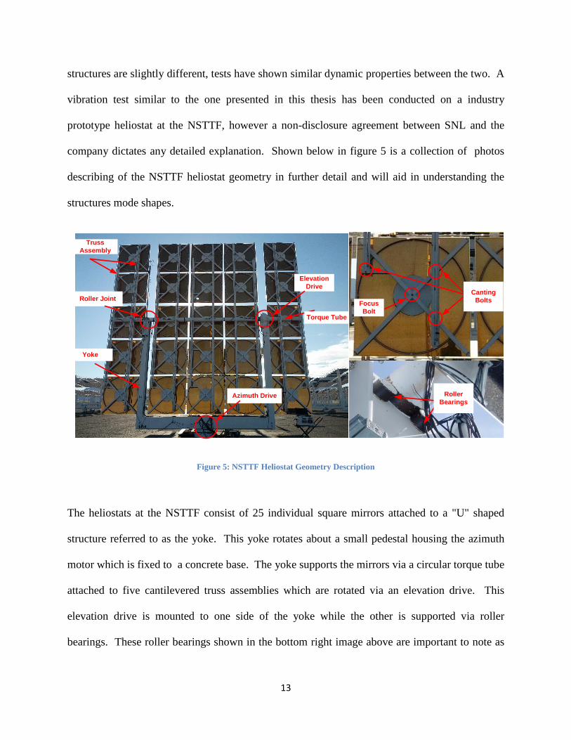
company dictates any detailed explanation. Shown below in figure 5 is a collection of photos
describing of the NSTTF heliostat geometry in further detail and will aid in understanding the
structures mode shapes.
Figure 5: NSTTF Heliostat Geometry Description
The heliostats at the NSTTF consist of 25 individual square mirrors attached to a "U" shaped
structure referred to as the yoke. This yoke rotates about a small pedestal housing the azimuth
motor which is fixed to a concrete base. The yoke supports the mirrors via a circular torque tube
attached to five cantilevered truss assemblies which are rotated via an elevation drive. This
elevation drive is mounted to one side of the yoke while the other is supported via roller
bearings. These roller bearings shown in the bottom right image above are important to note as
Torque Tube
Elevation
Drive
Azimuth Drive
Roller Joint
Truss
Assembly
Yoke
Canting
BoltsFocus
Bolt
Roller
Bearings

14
they do have a slight effect on the dynamics of the heliostat as the free rotation on one side
favors rotational motion about that point. Each truss assembly contains one short truss and one
long truss that both support five individual mirror facets. Each mirror facet has three adjustable
bolted connections to the trusses shown in the upper right image labeled canting bolts. These
bolts are used to individually tilt and aim the mirror facets about a respective axis to focus on a
single point. This process is called "canting" and is performed on every one of the 25 mirrors on
each heliostat. Also part of the mirror assembly is an adjustable bolt attached to the center of a
thin cylindrical plate which is adhered to the back of the mirror. This bolt can be slightly
adjusted and used to pull back and deform the mirror into a concave surface in a process called
"focusing". This process allows for better convergence of the reflected rays at the edge of the
mirrors essentially focusing a square beam shape into a circular one.
With all the adjustment and aiming required per heliostat, it quickly becomes apparent that this
geometry is difficult to model accurately in a finite element model. The first requirement set for
this model was the ability to re-produce the properly canted and focused heliostat mirrors based
upon the heliostat location with respect to the receiver tower. This means all 25 mirror facets
must be individually tilted and deformed prior to optical analysis. Also required is the ability to
rotate the heliostat model about a respective axis for any time of day. To build this model, a top
down approach was used in SolidWorks incorporating design tables for required inputs such as
heliostat location or elevation angle. With this top down model, it is possible to quickly and
automatically rebuild the model by simply changing the desired input values into the design table
which updates a reference geometry sketch. Parameters in this sketch are related to the
appropriate solid parts in the assembly, and thus rebuild the properly oriented heliostat when
changed. This methodology saves countless hours of remodeling the assembly and can be easily

15
implemented with some careful planning and a few additional steps during the models original
creation.
Static Testing
The first experiments at the NSTTF regarding FEM model validation sought after a validation
technique through the means of static testing. This static validation was performed prior to
attempting the problem of dynamic model validation which proves to be a more difficult task
[14]. Static testing was the first attempt at the NSTTF to validate a previously created model in
the SolidWorks CAD modeling software. This test was performed by very simply loading and
unloading the heliostat at certain locations while recording the displacements. The secondary
objective of this test was to determine the best method of statically testing and measuring
displacements on a heliostat. It was found that a ®Leica branded laser distometer, and a voltage
regulated string potentiometer provided the most accurate and precise measurements resulting
with an average uncertainty of +- 1.1%. By repeating the load at different locations with
different magnitudes and cross comparing to the displacements predicted by the SolidWorks
model, the connections and material properties were carefully modified to match the static
displacements. The main goal of this study was to verify the model correctly predicts gravity sag
in the structure for future optical simulations. Shown below in figure 6 is an example displaying
the FEM predicted displacements for a horizontally oriented heliostat due to gravity and a point
load at a strategic location on one of the trusses.
By reproducing this point load on a physical heliostat, the finite element model can be calibrated
to correctly match displacements measured at different locations on the deformed mirror facets.
This procedure was repeated with varying loads at different locations and provided data
necessary to obtain a statically calibrated model. The plot in figure 7 demonstrates the FEM

16
results before and after calibrating material properties and displays an improvement in
displacement approximation for one of the points tested. This static testing provided a good first
step in model validation, however geometric uncertainties and nonlinearities in the motor drives
need to be further explored as a dynamically verified model is ultimately desired.
Figure 6: Statically Loaded Heliostat Displacements from Early FEM Model
Figure 7: Measured and Modified FEA Displacements (Solidworks)

17
NSTTF Preliminary Modal Test
Shortly after the static displacement testing, a traditional modal test was performed in an effort to
prepare for a more robust installation and experiment which is the topic of this entire paper [2-3].
This prelimary test was conducted using previously developed and proven Sandia and
commercial modal analysis software. A range of accelerometers and strain gauges were tested
during this time to determine an optimum sensitivity for future procurement and test planning.
This resulted in the ultimate use of both DC MEMS and Piezo-electric accelerometers with
sensitivities of 1000 mV/G. With a low frequency range of 0-250 Hz, non-traditional DC
accelerometers (PCB 31713B112G) are reccommended to capture the low frequencies of any
rigid body motion associated with the two motor drives. The more inexpensive Piezo-electric
sensor (PCB 356M98, 0.5-3000 Hz) are also reccommended due to there low cost which helps
to increase the sensor count available for field deployment.
During this preliminary experiment, traditional hammer excitation was used to provide cleanly
defined mode shapes for comparison with FEM predicted shapes. In addition, some wind
excitated averages were taken to explore what modes are excited under windy conditions. It was
determined that the wind and hammer data sets produce the same fundamental frequencies, but
different damping values corresponding to wind speed. Also, as found by Gong et al, elevation
angle had little to no effect on resonant frequencies. These resonant frequencies were also found
to lie within the three wind speed spectrums described by the earlier Google sponsored work, and
further verified the need for modal characterization of wind excited modes.
Utilizing previously predicted mode shapes from the Solidworks model, there was enough
vibration data to match a majority of the first ten modes with minimal frequency errors. An
example of this early mode shape identification is shown in figure 8 below comparing an

18
experimental and FEM predicted modes shape. It also became apperent that there exists a couple
of rigid body modes that are not predicted by the model. There was also more discrepency in the
higher frequency calculations which suggests a more accurate model may need to be created.
This was expected as the heliostat FEM model was created with very simple solid masses
representing the elevation and azimuth motors, along with other simplifications that were not
determined important at the time of the models creation. This preliminary experiment provided
the groundwork needed to determine an approporiate instrumentation set required to perform a
more detailed and permanent modal monitoring study of the NSTTF heliostats. It also provided
a well determined set of physical mode shapes with which to compare with the FEM predictions
and future tests. This preliminary test also verified and ideal set of sensor locations for modal
parameter estimation which will be used to provide more detailed shapes in future analysis.
Thanks to the modal lab at Sandia National Laboratories, the NSTTF was able to move forword
with costly data acquisition and sensor procurement with confidence. All sensors and equipment
used in this research was funded by the Amercian Recovery and Re-Investment Act (ARRA)
stimulus funding.
Figure 8: Preliminary Modes (Left) FEM = 1.604 Hz, (Right) EMA = 1.634 Hz

19
After the preliminary modal test was conducted, it was decided the SolidWorks FEM was too
in-efficient with regards to computation time and in-accurate when comparing higher frequency
modes. To combat these issues, the model was modified to run in Ansys Mechanical which
allowed for better parallel processing and more detailed parameter controls. Other modifications
such as custom controlled roller joints are applied to the motor drive which in turn added the
rigid body motion witnessed in the preliminary modal analysis. The first step in duplicating the
NSTTF heliostat in an FEA model is to correctly aim and focus the heliostat. As previously
mentioned, each of the individual mirrors has to be tilted and focused based on the heliostat
position with respect to the intended aim point and day of interest. For the optical results
presented in a later chapter, all ray tracing was performed for various times on March 21st which
reflects the day at which this model was intended to be focused thus creating an ideal condition
with regards to the reflected beam. To correctly focus the individual mirrors, an initial static
analysis is performed where 25 individual displacements are applied to the center of the mirrors
similar to what is done in real life via the focus bolt. This displacement is applied according to
the focal length of the mirror which is a function of the distance between the heliostat and the
receiver target. This is better shown the figure 9 below depicting this heliostat focusing
technique applied to the FEM in Ansys Mechanical. After applying this deformation and gravity
pre-stressing, this model is now ready to be compared and calibrated to match operational modal
results acquired from this research.

20
Figure 9: (Left) Forced Displacements in Static FEM model; (Right) Dispacement Results for Static Heliostat
Data Acquisition and Instrumentation
Well Instrumented Heliostat
The main focus of this research will be on one specific heliostat located on the eastern edge of
the heliostat field with the NSTTF field designation 11W14 corresponding to its row and
location with respect to the tower. This heliostat referred to as the "well instrumented heliostat"
contains a total of 24 tri-axial accelerometers, six ultrasonic 3D wind anemometers, and six
dynamic strain gauges. This heliostat was chosen to instrument heavily as an attempt to fully
characterize the heliostats mode shapes at a high enough resolution to best match FEM predicted
mode shapes. Along with the accelerometers, the dynamic strain gauges and high speed wind
anemometers will aid in future analysis performed at the NSTTF ranging from fatigue modeling
to wind profiling and verification of computational fluid dynamics models. Figure 10 below
demonstrates the placement of these sensors on the heliostat as well as a photo of one of two
wind sensor towers assembled near the heliostat. Based on the previous experimentation, the
sensors chosen to instrument heliostat 11W14 are low frequency range DC MEMS
accelerometers (PCB 31713B112G) which have a frequency range of 0-250 Hz. This low
frequency requirement is made based on two rigid body modes that exist at relatively low

21
frequencies. These rigid body modes exist because of the backlash and non-linearities seen
inside the elevation and azimuth drives. The low frequency capability of these sensors allows
the system to capture these modes that are assumed to be excited by low wind speeds and
heliostat movement during operation. These sensors are mounted on the heliostat via magnetic
mounts and are shown as red and blue cubes in figure 10. The blue box represents a reference
sensor for cross-spectrum analysis with respect to all other sensors.
These sensors are placed at the extremeties of the trusses and yoke which are known to give the
largest displacement during mode excitation. The green circles in the figure represent dyanamic
strain gauges which are glued to the torque tube after properly sanding and smoothing the
surface. These sensors help to provide further modal verification and will be used in the future
with tradiational strain gauges for wind load approximation. The wind sensors used are high
speed 3D Ultrasonic Anemometers (R.M. Young 8100) which measure wind speed, direction,
elevation,and temperature at 32 Hz. These anemometers are mounted on nearby towers at three
different height in order to capture up stream wind speed and the wind speed directly behing the
heliostat. As previosly mentioned in the Google work, monitoring wind at such high speeds is
necessary to capture the wind gusts or any turbulance created by adjacent heliostats. These wind
towers are portable and can be moved with a forklift to any heliostal laocation in the field if
future analysis dictates it.

22
Figure 10: (Left) Well Instrument Heliostat Instrumentation Layout; (Right) Photo of Up-Stream Wind Anemometer
Tower
All these sensors are routed into the weather-proof data acquisition enclosure at the base of the
heliostat shown in green which houses all acquisition and communication hardware. With such a
large channel count, high speed requirements, and remote location, the data acquisition itself
presents some unique challenges. Using all National Instruments hardware and LabVIEW
software, this system was custom created to sync all sensors together and stream real time data to
the NSTTF control tower or any heliostat location with the use of a laptop. Including wind,
strain, and acceleration, the well instrumented heliostat contains 102 channels of streaming data
across more than 1300ft of buried fiber optic cable. NI Compact RIO hardware was
programmed to sync all channels, perform necessary signal conditioning on the FPGA (Field
Programmable Gate Array), and stream the data remotely to a control computer where data is

23
further analyzed and logged. The FPGA structure built into the Compact RIO's hardware is a
very useful tool as it allows for standalone processing on the cRIO unit without the need for a
host computer. This allows for a majority of the signal processing to be performed prior to
streaming the data thus reducing lag on the host PC or possible bottle-necking of large data
packets. Figure 11 below is an illustration of the cRIO hardware residing in the well
instrumented heliostat DAQ enclosure at the base of the heliostat. Due to the large channel
count on the well instrumented heliostat, a total of three cRIOS had to be deployed together
within the single heliostat enclosure and custom synced together. To ensure the channels are
logging on the same time signature, a digital input / output module had to be used to export the
clock trigger of a "master" cRIO to that of two "slave" cRIOS. This digital trigger ensures the
channels on the two slave chassis's record at the same time as the master cRIO and eliminates
possible errors that may be otherwise seen in the logged data. Also included in the DAQ box but
not shown here is an Ethernet switch used to link this system to the existing heliostat controls
and a DC power bus which provides power to all data acquisition hardware as well as the DC
accelerometers and six wind anemometers. All instrumentation and hardware is powered by
existing heliostat electrical runs, and thus the system only works while heliostat power is turned
on.
cRIO
9073
8 Slot
Chassis
Master
cRIO
9073
8 Slot
Chassis
Slave
cRIO
9073
8 Slot
Chassis
Slave
X Accel.
Y Accel.
Z Accel.
Hammer
Strain
Wind
Digital I/O (Sync)
Figure 11: Wiring Diagram of DAQ Hardware

24
Field Instrumentation & Data Acquisition
To study the blockage effect of frontal heliostats on interior heliostat wind excited vibration, a
set of nominally instrumented heliostats are co-located near or around the well instrumented
heliostat. These heliostats contain a total of four DC or Piezo-electric tri-axial accelerometers
mounted on the four outermost trusses and a single strain gauge mounted on the torque tube. A
select few heliostats also contain a heliostat mounted wind anemometer attached to the yoke and
extending to the top of the heliostat mirror facets. In total, 13 heliostats have instrumentation
including one heliostat on the western end which only monitors wind speed. As shown in figure
12, the triangular block of heliostats was chosen behind heliostat 11W14 in order to capture
predominant south-western wind which is expected at this location. The yellow blocks represent
these nominal heliostats where the blue ovals correspond to locations where wind speed is
measured. Over time, these individual heliostats will provide a wind excitation profile linking
wind speed and field location to wind excited magnitudes. This information will shed light on
interior heliostat vibration, and whether or not heliostat induced turbulence is a factor on interior
heliostat mode excitation. This information can then be better used to analyze optical losses and
verify previous wind load and blockage models.
Figure 12: (Left) Field Deployment Map of Instrumented Heliostats; (Right) Alternate View of Instrumented Heliostats

25
With such a complicated experimental setup and unique requirements, custom software was
written in the LabVIEW programming environment to stream and log any necessarry data. To
first verify the programming procedure works as desired, a test program was written to perform
operational modal analysis on a simple free-free condition beam. This steel beam shown in
figure 13 was suspended via elastic bands and instrumented with eight tri-axial accelerometers
and utilizes the same data acquisition hardware as was installed on the full heliostats. The
program written utilizes the same cross-spectrum technique and random excitation theory as used
in the heliostat analysis and was proven to work well on this simple case study. The cross
spectrum analysis performed in the DAQ program is especially usefull when no input signal is
available and allows for relatively good modal approximation for operational modal analysis, but
does require a larger amount of averages for clear results. This calculation is sometimes referred
to as the auto power spectrum and follows equation 1 for each degree of freedom in the system.
𝐶𝑟𝑜𝑠𝑠 𝑃𝑜𝑤𝑒𝑟 𝑆𝑝𝑒𝑐𝑡𝑟𝑢𝑚 𝑆𝐴𝐵 𝑓 =𝐹𝐹𝑇 𝐵 ∗𝐹𝐹𝑇(𝐴)
𝑁2 (1)
This preliminary system was developed at the University of Wisconsin, Madison to first verify
the method and hardware used is succesfull in identifying operational mode shapes of a structure.
This test setup was performed prior to undertaking the much more detailed program required for
the full heliostats in order to provide the confidence needed to purchase the data acquisition
equipment and large array of sensors. Without going into too much detail, this beam test resulted
in the required frequency data and mode shapes and thus provided a backbone program to build
upon. The first two mode shapes of the beam are plotted in figure 14 below for reference and
were obtained using random excitation from a standard instrumented hammer not hooked into
the data acquisition system. These operating shapes were found by the same random excitation

26
technique used on the full heliostat which will be discussed further in the operational modal
analysis chapter. Also tested but not presented here was the dynamic response of a downhill ski
which produced similar results further verifying the system was working as intended.
Tri-axial Accelerometer
Steel Beam
Compact RIO
Figure 13: Experimental Set-Up for Preliminary Data Acquisition Test
Figure 14: First Two Bending Modes of Beam Obtained from OMA Techniques
This simple beam acquisition system allowed for confidence in building a much larger and more
complicated program with the goal of monitoring and logging heliostat vibration data from all 13
instrumented heliostats previously mentioned. To do this, the data acquisition program was
0 5 10 15 20 25 30 35 40-0.4
-0.3
-0.2
-0.1
0
0.1
0.2
0.3
0.4
0.5
0.6Mode Shape
X Position
Modal A
mplit
ude
0 5 10 15 20 25 30 35 40-0.8
-0.6
-0.4
-0.2
0
0.2
0.4
0.6Mode Shape
X Position
Modal A
mplit
ude

27
separated into two separate sub-routines; one pertaining to the well instrumented heliostat and
the other pertaining to all remaining nominal heliostats. The first program is used to fully
characterize the dynamics of the well instrumented heliostat and provide the data needed finite
element model verification for use in the optical portion of this analysis, while the nominal
system will be used to acquire data for future analysis not presented here.
The well instrumented program shown in the left screenshot of figure 15 monitors and logs data
from all 102 channels streamed in real time from heliostat 11W14. Due to the large amount of
data required and the desire to not interfere with heliostat operation and testing, a dedicated
fiber-optic line is used for communication between the control tower and heliostat 11W14. This
communication line provides high speed portal needed to stream acceleration data collected at
rates up to 52 kHz without any issues or holdups. Included in this program is the ability obtain
the heliostats current orientation by linking into the heliostat control network, and is also able to
monitor individual channels for debugging purposes. This is inherently helpful as the heliostat is
constantly moving and snagged cables quickly become a reality. This system allows for logging
of acceleration, strain, wind speed and direction data in the time or frequency domain. With
respect to the frequency analysis, all required averaging or zooming parameters are user
controlled and output data either in real / imaginary or magnitude / phase format. Based on the
preliminary modal analysis performed at the NSTTF, the frequency range of interest is set to
zero to twenty hertz with a line resolution of 3200 which is equal to a frequency resolution of
0.00625 Hz.
To monitor the rest of the nominally instrumented heliostats, data can be bundled onto a single
phase of the three-phase power line used at each heliostat. This communication protocol which
already exists, is used currently to control the heliostats position, and provides a communication

28
portal as long as the data packets being sent are of a reasonable size. To monitor these additional
12 heliostats, a separate data acquisition program was written which can be ran in parallel with
the well instrumented heliostat program. Since these nominal heliostats lack the high fidelity
measurements required for mode shape representation, this program monitors the power spectral
density and time domain data of each accelerometer instead of the cross power spectral density
seen in the higher fidelity well instrumented heliostat system. Along with wind and strain
measurements, this data will in time help to provide enough information to characterize wind
excitation as a function of field position and frontal heliostat blockage. A screenshot displaying
this power spectra for each of the nominally instrumented heliostats is also shown below in
figure 15. The use of these two systems allows the engineer to examine wind excitation in real
time, and provides a robust program to build upon in the future.
Figure 15: (Left) Well Instrumented Heliosta DAQ Screenshot; (Right) Nominal Heliostat DAQ Screenshot
Operational Modal Analysis Part one of this overall heliostat study is to experimentally measure the operational mode shapes
excited by the wind often referred to as operating deflection shapes. With respect to the
operational modes of interest, we consider a static "non-operating" heliostat in any said
orientation that is subject to wind excitation. Any motion or movement due to motors is

29
therefore ignored although this vibration would most likely only effect the rigid body modes
which are discussed in the results chapter. At the mercy of windy days, a pseudo random input
was used to simulate the forcing function of the wind. This random input is introduced with a
standard instrumented sledge hammer normally used in experimental modal analysis. This input
was provided to the trusses and yoke in a manner which to excite the same modes excited during
a wind event. This process included roaming the force input from truss to truss while averaging
the response data. The force was varied across both top and bottom portions of the truss for
three different heliostat orientations chosen to best represent an operating heliostat. The force
was repeated in different directions after allowing the initial response to dampen out and follows
the same random excitation methodology used in the simple beam case study mentioned
previously. This method was determined acceptable after noticing a similar response from a
collection of early wind excited data that was available, and thus it was concluded that random
excitation is a good stand in for wind excitation and allows for faster data collection. This
methodology will be further examined along with some early wind excited data sets in a later
chapter as it concerns modal amplitudes.
One of these random excitation tests takes approximately 4-5 hours to conduct and only requires
one test engineer, a laptop, and a motorized man-lift. This testing method is much faster than
waiting for a windy day which may or may not happen when needed, and provides for a more
controlled experiment. Figure 16 displays the cross spectrum of a random excited data set
compared to a operational wind excited data set taken during wind events averaging at
approximately 18 and 30 mph. Early wind excited data sets show this random excitation
technique does indeed excite the same modes, however the modal magnitude was found to vary
with wind speed as a higher force leads to a larger magnitude mostly in the low frequency

30
modes. The red plot represents cross spectra from random excitation input while the green and
blue are the cross spectra from the averaged wind excited data overlaid onto the random
excitation data for the compiled Z DOF response. As shown in this plot, random excitation is
found to be a good replacement for wind excited mode approximation, however wind speed
profiling is still very important when considering displacement magnitudes. This wind excited
magnitude becomes more important when considering optical characterization and will be
explored further with the limited wind excited data that is available, however for purposes of
modal characterization, the random OMA process is used to provide the mode shapes discussed
in the research.
Figure 16: Wind Excited Data (blue / green) vs. Random Excitation Data (red)
To extract the operational mode shapes from the cross spectrum data, a total of 20 data sets per
orientation are averaged with frequencies ranging from zero to twenty hertz with a resolution of
.00625 Hz. This data is compiled into three averaged data sets for each orientation
corresponding to the "X", "Y", and "Z" DOF's for modal parameter extraction. The modes are

31
then determined individually using an automatic algorithm of mode isolation in Matlab [15] and
plotted next to the finite element counterpart for shape comparison. Due to the presence of
closely spaced modes and operational noise, the modes must be individually isolated in the curve
fitting process. It is also important to isolate modes in the correct DOF data set based on the
maximum expected motion seen in the mode shape. For example, a mode shape where motion in
the Y DOF is dominant, than the Y DOF data set will provide the cleanest looking shape whereas
the Z DOF may not correctly represent this mode. The plot below in figure 17 demonstrates this
isolation for a single mode around 3.2 Hz in the Z DOF data set. By repeating this process for
each mode in each of the three degrees of freedom, one can plot and match the mode shapes to
their finite element counterpart.
Figure 17: Algorithm of Mode Isolation Curve Fitting Process
When plotting mode shapes of such a structure that rotates, it is important to keep track of the
orientation as the majority of the sensors rotate at an angle θ with respect to the horizontal. This
can get rather tricky during modal analysis as there can exist multiple coordinate systems which
makes mode shape comparison very difficult if not impossible when plotting experimental
1.5 2 2.5 3 3.5 4 4.5 5 5.5 6 6.5
10-10
10-9
10-8
10-7
Frequency (Hz)
Composite of Residual After Mode Isolation & Refinement
Data
Fit
Data-Fit
0 0.2 0.4 0.6 0.8 1 1.2 1.4 1.6 1.8
x 10-5
0
0.2
0.4
0.6
0.8
1
1.2x 10
-20 Complex Sum(abs) FRFs
Re{H()}
Im{H
()}
Data
Fit

32
shapes. A transformation procedure to map the sensor locations in three dimensional space is
outlined in figure 18 and equation 2 for use in mode shape plotting. This equation relates the
measured frequency response and elevation angle of the heliostat to physical Cartesian
coordinates which are used for plotting 3D mode shapes in Matlab. It is easy to see the
importance of the elevation angle when plotting mode shapes as the global Y and Z deflections
are a function of both the X and Z measurements as well as the elevation angle, θ. As mentioned
before, mode isolation is performed on a single DOF bases, and thus the modal magnitude of the
remaining DOF''s is the interpolated response at the same frequency. For orientations where this
response is seen in two or more DOF's, the response with the largest magnitude and clearest
mode shape is used for mode isolation.
To correctly map the modal coordinates from the test data to physical coordinates representing
the heliostat, equation 2 correlates the static position of each DOF, 𝑞0 with the deformed position
𝑞𝑖 where 𝜙𝑡 is the measured response of the isolated mode at the corresponding truss location
and 𝑀𝑋 is a arbitrary magnification factor for visualization purposes. This equation along with
static sensor coordinates obtained from the finite element model allows for a 3D plot
representing sensor DOF locations. Figure 18 also shows an example plot of the heliostat in the
45 degree orientation with the measurement nodes connected for visualization purposes. A
comparison of the experimental mode shapes with initial FEM predictions are presented using
this style in the results section.

33
Figure 18:Coordinate Description and Plot Reconstruction of Heliostat Nodes.
𝑞𝑖 =
𝑞𝑖 ,𝑥
𝑞𝑖 ,𝑦
𝑞𝑖 ,𝑧
=
𝑞𝑥0
𝑞𝑦0
𝑞𝑧0
+
𝜙𝑡𝑌
𝜙𝑡𝑍𝑐𝑜𝑠 90 − 𝜃 − 𝜙𝑡𝑋𝑐𝑜𝑠 𝜃
𝜙𝑡𝑍𝑠𝑖𝑛 90 − 𝜃 + 𝜙𝑡𝑋𝑠𝑖𝑛 𝜃
𝑀𝑋
𝑀𝑌
𝑀𝑍
(2)
Thanks to previous modeling efforts and preliminary experimental modal testing, finite element
predicted shapes are available for aiding in mode shape verification. The model can now be
further verified with newly acquired detailed mode shapes and is capable of creating deformed
mode shapes of the NSTTF heliostat at any configuration or field position for use in optical
analysis. As mentioned in an earlier chapter, field position is important parameter as every
heliostat must be initially aimed and focused to its target, thus creating slightly different mirror
geometry. Once this model is created, the first 30 mode shapes are solved incorporating gravity
pre-stressing and mirror focusing. These deformed shapes and modal test data will then be used
for fatigue analysis and ray tracing studies as well as a number of future design optimization
studies at the NSTTF. To verify this model, operational modal analysis was performed on the
well instrumented heliostat in three different orientations. The three orientations of current
interest are a vertical position or 90 degrees where all mirrors are in plane with the yoke support,
tXtZ
yX
yZY
Z
X
tY
yY
iq
-100
0
100
200
300
-100
-50
0
50
1000
50
100
150
200
250
X
Node Locations
Y
Z

34
a more realistic operational orientation of 45 degrees, and the stow configuration which is six
degrees with respect to the horizontal. The vertical orientation will be presented in this paper
which provides easy to interpret shapes, while the other two data sets provide useful information
regarding heliostat orientation and excitation magnitudes for use in future analysis.
OMA and FEM Results
It has been shown by both experimental results and the FEM results that there exists two major
type of modes labeled as in plane bending modes and out of plane bending or twisting modes.
The distinction between these two types of shapes in important as the out of plane modes are
assumed to present a larger deflection with respect to the reflected beam. To quantify this
optical error, the shapes provided by the finite element model are matched with the operational
mode shapes that are measured with this new dynamic monitoring system. Once validated, the
deformed shape is then exported to a ray tracing code to determine how much flux is lost at the
instance of modal excitation.
With complicated structures such as the NSTTF heliostat, it is easier to isolate mode types or
groups in order to better understand the dynamic behavior. In addition to in plane or out of plane
motion, the shapes will be further broken down depending on which portion of the structure is
responsible for the motion. These categories are broken into the following three mode
categories; torque tube bending modes, torque tube torsion modes, and yoke bending modes. In
addition to these modes, there exists two rigid body modes that occur due to backlash or "slop"
in the elevation and azimuth motors.
The rigid body modes account for rotation about the elevation and azimuth axis and are
relatively low in frequency at around .88 Hz and 1.23 Hz respectively. The rigid body mode

35
responsible for rotation about the azimuth drive was found to vary with heliostat orientation and
is the only mode to do so. Early results verify this behavior on both the NSTTF heliostat as well
as two commercial prototype heliostats tested at SNL which aren't presented due to non-
disclosure agreements. This is intuitively true as the natural frequency of this mode is
dependent on moment of inertia about the vertical axis which is changed as the mirrors rotate.
To demonstrate this behavior, the natural frequencies were reconstructed at various orientations
using inertia properties from the FEM model. The plot shown in figure 19 displays the moment
of inertia across the relative axis and the reconstructed frequencies using equation 3 where 𝑘𝜃and
𝐼𝜃are the rotational stiffness and inertia about the drive axis. This approximation may be off
slightly as the FEM model still contains uncertainties regarding material properties, but the trend
matches experimental data well for the three orientations measured. This educational example
helps to differentiate the two rigid body modes from one another and explain the reason behind
rigid body frequency dependence on heliostat elevation angle.
Figure 19: Heliostat inertia and rigid body Frequency Vs. Elevation Angle
𝑓 =1
2𝜋
𝑘𝜃
𝐼𝜃 (3)
0
0.2
0.4
0.6
0.8
1
1.2
1.4
1.6
1.8
2
0.0E+00
1.0E+07
2.0E+07
3.0E+07
4.0E+07
5.0E+07
6.0E+07
7.0E+07
8.0E+07
0 20 40 60 80 100
Mo
me
nt
of
Ine
rtia
(lb
s*in
^2
)
Heliostat Orientation (deg, 0 deg = Horizontal)
Inertia Vs Frequency of Rigid Body Modes
Izz (Azimuth)
Iyy (Elevation)
fn2 (Azimuth)
fn1 (Elevation)
Fre
qu
en
cy(H
z)

36
This conclusion can be beneficial to designers as every modern heliostat contains two motors
which than correspond to these two rigid body modes. This information is also useful as the
current FEM model of the NSTTF heliostat is simplified with respect to the two motor drives.
These two motors are modeled as solid masses in the FEM and thus do not capture this behavior
exactly, however rotational contact conditions are applied to the nodes that make up these solid
masses and do a relatively good job simulating these rigid body mode shapes. The low frequency
mode associated with the elevation drive is especially important as early wind excited data sets
shows excitation of this mode heavily at approximately .88 Hz, where as the azimuth rigid body
mode is only slightly excited. For the majority of the non rigid body modes predicted by the
finite element model, there was good agreement between the Ansys predictions and the test data.
All non-rigid-body modes were found to not vary much with heliostat orientation as found in
previous research. Table 2 below is a list of the first 22 predicted and measured modes along
with a simple shape description for the vertical orientation data set. These initial results are fairly
accurate for the majority of the modes, although some modes do have a rather large discrepancy,
most notably in the higher frequency modes. It was also determined that there exists very similar
and closely spaced modes that are grouped into mode "families". Some of these modes
belonging to the mode families highlighted in yellow and orange in table 2 are sometimes not
found in the operational data and are assumed to be lost in noise or overly-dominated by one of
the single modes. The repeated modes may also result from numerical errors in the FEM model
and are assumed to have a the same excitation of the mode found in the OMA analysis. Also
plotted below the table in figure 20 is a bar graph of these two results for comparison purposes.
Since this paper is not specifically concerned with modal validation of finite element models,
this error in frequency was deemed acceptable as long as the shapes match correctly.

37
Mode Number
Ansys Wn (hz)
OMA Wn (Hz) Motion
Description
1 1.129 0.8832 Rigid body
rotation Rotation about elevation axis
2 1.605 1.639 In plane Yoke bending
3 2.991 3.11 In plane Torque tube bending
4 3.2884 3.2418 Out of plane Torque tube twisting
5 3.299 3.242 Out of plane Yoke twisting
6 3.578 4.03 In plane
Combination of trusses bending in and out of phase. All motion is in plane and
consists of only truss motion.
7 4.1034 4.1273 In plane
8 4.2563 4.1273 In plane
9 4.4299 4.1273 In plane
10 4.5168 4.1273 In plane
11 4.5925 4.1273 In plane
12 4.6084 4.4961 In plane
13 4.6295 4.6583 In plane
14 4.6396 4.1263 Out of plane Trusses bending in and out of phase. Minimal truss "twisting". 15 4.6529 4.1263 Out of plane
16 5.2021 5.6109 Out of plane Trusses twisting in and out of phase
17 5.4822 6.03 Out of plane
18 6.5285 6.6352 Out of plane Torque tube bending
19 7.0587 7.1018 Mixed Yoke and truss bending
20 7.1692 8.6147 Out of plane
Truss twisting 21 7.1843 9.019 Out of plane
22 7.7 9.38 Out of plane Table 2: FEM and OMA Modal Frequency Comparison
Figure 20: OMA and Ansys Mode Comparison Plot
0
1
2
3
4
5
6
7
8
9
10
1 2 3 4 5 6 7 8 9 10 11 12 13 14 15 16 17 18 19 20 21 22
Frq
ue
ncy
(H
z)
Mode Number
Ansys - OMA Frequency Comparison
Ansys Wn (hz)
OMA Wn (Hz)

38
The following figures (21-23) contain a few plotted examples of predicted mode shapes versus
measured shapes categorized by the different types of modes. The rigid body mode
demonstrated in figure 21 is simply the rotation about the elevation axis where rotational hinge
joint contacts were added in the model. It is hard to see in this image, but this rotational spring
contact is responsible for a slightly larger deformation on the side of the heliostat which is not
constrained by the elevation motor. This may seem like a small detail, but the importance can be
seen when one considers the reflected beams offset which is only magnified with distance to the
receiver. This behavior has been noticed on larger commercial scale heliostats located at the
NSTTF where the large area acts as a sail thus easily exciting these rigid body modes. During
these wind events, the small rotation seen in the rigid body modes of the heliostat due to gear
backlash in the motors leads to a very large offset of the beams centroid. This lends one to
believe that a long range heliostat at distances over a mile may reflect the beam and completely
miss the target on a windy day. This assumption still needs further research, but could possibly
lead to large savings in future plant designs.
Figure 21: (Left) Ansys Mode #1, 1.13 Hz; (Right) OMA Mode #1, 0.88 Hz
-1000
100200 -150
-100-50
050
100150
0
50
100
150
200
250
300
HZ
Natural Frequency (Hz):0.88316
HX
HY

39
The other modes depict examples of the in plane and out of plane mode shapes which are best
matched with the operational mode shapes. One negative side effect of operational modal
analysis is the addition of noise and need for many averages. This error becomes apparent as it
is sometimes difficult to obtain cleanly plotted mode shapes, however thanks to the previous
SIMO (Single Input Multi-Output) tests performed as part of our preliminary modal test, there is
confidence in mode shape characteristics. The best method to match these shapes is to link the
participating member or truss and its phase with respect to the other members. In other words,
one can match modes based on one physical truss bending or twisting in or out of phase with its
neighbor truss. The first type of mode is shown below in figure 22 and is due to bending or
twisting in the yoke members. Shown in this mode is in-plane bending about the "soft" direction
of the I-Beam members of the yoke support. This mode essentially translates the mirrors in
plane and in phase with one another, and also incorporates the rigid body rotation about the
elevation drive seen in figure 21 There also exists a yoke twisting mode which contributes to out
of plan motion and can be seen in the appendix where the first 22 modes are listed.
Figure 22 (Left) Ansys Mode #2, 1.61 Hz; (Right) OMA Mode #2, 1.64 Hz
-100-50050100150200250
-100
0
100
0
50
100
150
200
250
300
HZ
Natural Frequency (Hz):1.6386
HX
HY

40
The remaining modes of interest are broken into two categories; in-plane and out-of-plane
motion of the mirror facets. The in-plane modes are mostly due to the bending modes of the
circular torque tube. Figure 23 shows the effect of the torque tubes first fundamental bending
mode on its attached mirrors. This trend is seen in higher frequency modes where the same in-
plane motion is observed as the mirrors vibrate in and out of phase with each-other due to higher
frequency bending in the torque tube. The out of plane modes can possibly be attributed to un-
equal truss lengths or possibly torsion in the torque tube as the motion is due to a twisting
phenomena about the central axis of the five mirror assembly. This mode type shown in figure
24 occurs at higher frequencies and contain the highest magnitude of excitation next to the
azimuth rigid body mode shown in figure 21. While there were two other out of plane modes
corresponding to the yoke or torque tube bending, the majority of out-of-plane motion seen can
be attributed to these truss twisting modes. This gives insight to possible future design
modifications that will alter this mode shape or frequency with the hope of improving heliostat
performance by reducing this excitation or eliminating the mode altogether by effective damping
methods.
Figure 23: (Left) Ansys Mode #4, 3.28 Hz; (Right) OMA Mode #4, 3.24 Hz
-100-500501001502002500
50
100
150
200
250
300
HX
Natural Frequency (Hz):3.2418
HY

41
Figure 24: (Left) Ansys Mode #16, 5.20 Hz; (Right) OMA Mode #16, 5.61 Hz
Optical Ray Tracing and Plant Performance A common practice in concentrating solar technologies is the use of ray tracing codes for optical
performance calculations and optimization. ®APEX is a commercial software package produced
by Breault Research group which utilizes proven ray tracing code and exists as a third party
plug-in tool for the SolidWorks CAD environment. This tool makes ray tracing much easier by
introducing an intuitive GUI as opposed to the traditional scripting language which contains a
steep learning curve. This tool also makes it possible to construct a re-configurable "Top-Down"
assembly replicating any said heliostat, or in theory an entire heliostat field, within a SolidWorks
assembly. Due to current computing resources available at the NSTTF, a full field within APEX
has not been tested, but exists as a future possibility. The NSTTF staff do however have a other
non visual methods of calculating performance of an entire plant which run much faster.
Simulations using one of these performance codes will be presented for the NSTTF field in a
later section, but for this portion of the study, the results presented are only concerned with the
flux contribution from a single heliostat undergoing wind excited vibration.
-100
0
100
200-150
-100-50
050
100150
0
50
100
150
200
250
300
HZ
Natural Frequency (Hz):5.6109; Damping = 0.0020671
HX
HY

42
Miles Equation
The first step in this proposed optical modeling method is to output the deformed mode shapes
computed by the Ansys simulations. To accomplish this, a script was written in Ansys APDL
which automatically scales and saves the deformed mode shape meshes after running a modal
simulation. In order to save computation time, only the surfaces of the 25 deformed mirrors are
exported as these surfaces are the only reflective surfaces required for ray tracing. Before
outputting this deformed mesh, one must equate a scale factor regarding the FEM displacement
which are arbitrarily scaled for visualization purposes. A realistic displacement can be
approximated from the operational data and is used to define a scaling ratio of the test
displacements to the arbitrary one output from Ansys.
In 1954, John W Miles defined an equation relating the frequency response of a single degree of
freedom system to the root mean square acceleration, displacement, or force at that degree of
freedom [16-17]. This relation was defined in an effort to better understand stresses in structural
aircraft components that are introduced to wind gusts or random loading. Shown below in
equation 4, one can approximate the rms acceleration, 𝐺𝑅𝑀𝑆 , using the data acquired previously
where 𝐴𝑆𝐷𝑖𝑛𝑝𝑢𝑡 is the randomly excited acceleration power spectrum with units of 𝑔2
𝐻𝑧.
𝐺𝑅𝑀𝑆 = 𝜋
2𝑓𝑛𝑄[𝐴𝑆𝐷𝑖𝑛𝑝𝑢𝑡 ] (4)
𝑄 =1
2𝜁 (5)
Thanks to the Miles equation, an approximated rms acceleration can be found from the randomly
excited frequency data, but for ray tracing purposes, the displacements are required. Thankfully,
this is easily obtained by converting the accelerations power spectrum to a displacement
spectrum in a process sometimes referred to as "omega arithmetic". After a short derivation

43
shown below in equations (6a-6i), the displacement spectra is easily found by dividing the
acceleration spectra by −𝜔2 [18]. Applying this procedure with Miles equation, one can then
obtain an approximate displacement for each degree of freedom in our test data using equation 7.
𝑥 𝑡 = 𝑋 𝑓 𝑒 2𝜋𝑖𝑓𝑡 𝑑𝑓∞
−∞ (6a)
𝑥 𝑡 = 𝑋 𝑓 𝑒 2𝜋𝑖𝑓𝑡 𝑑𝑓∞
−∞ (6b)
𝑥 𝑡 = 𝑋 𝑓 𝑒 2𝜋𝑖𝑓𝑡 𝑑𝑓∞
−∞ (6c)
𝑥 𝑡 =𝑑
𝑑𝑡 𝑥 𝑡 (6d)
𝑥 𝑡 =𝑑
𝑑𝑡 𝑋 𝑓 𝑒 2𝜋𝑖𝑓𝑡 𝑑𝑓
∞
−∞ (6e)
𝑥 𝑡 = 𝑋 𝑓 𝑑
𝑑𝑡 𝑒 2𝜋𝑖𝑓𝑡 𝑑𝑓
∞
−∞ (6f)
𝑥 𝑡 = 2𝜋𝑖𝑓𝑋 𝑓 𝑒 2𝜋𝑖𝑓𝑡 𝑑𝑓∞
−∞ (6g)
𝑋 𝑓 =𝑋 (𝑓)
𝑖𝜔 (6h)
𝑋 𝑓 =𝑋 (𝑓)
−𝜔2 (6i)
𝐷𝑅𝑀𝑆 = 𝜋
2𝑓𝑛𝑄
𝐴𝑆𝐷𝑖𝑛𝑝𝑢𝑡
−𝜔2 (7)
By writing this procedure into the mode isolation algorithm, approximate displacements of each
DOF for each mode excited can be found. An example of these calculated DOF displacements is
plotted in figure 25 below for a single mode at approximately 4.13 Hz. This type of plot was
created for every mode excited in the operational data set and is included in the appendix. By
tabulating the maximum displacement seen per mode and the arbitrary displacement obtained
from Ansys, the required displacement scale factor can found and used to properly output
deformed shapes. From this analysis, the largest displacements were seen in the elevation rigid
body mode, and some higher frequency out of plane modes ranging between 5-25 mm. A bar

44
plot representing the maximum displacement of the heliostat in the vertical orientation is
approximated by the miles equation and shown in figure 26.
Figure 25: RMS Displacements for Mode #14
Figure 26: Maximum Displacement Per OMA Mode Shape Aproximated with Miles Equation
0 5 10 15 20 250
0.5
1
1.5
2
2.5
3
3.5
4
4.5
5x 10
-3
DOF #
Dis
pla
cem
ent
(m)
Recovered Miles RMS Displacement wn = 4.1263Hz
Max Steady Disp = 0.0047754 m
0
0.005
0.01
0.015
0.02
0.025
0.03
1 2 3 4 5 6 7 8 9 10 11 12 13 14 15 16 17 18 19 20 21 22
Max
imu
m D
isp
lace
me
nt
(m)
Mode Number
Maximum Miles Displacement per Mode Shape

45
Wind Displacement Approximation The above displacement approximations were performed on the random excitation data set
correspoinding to the heliostat in the vertical orientation. To further examine the displacements
cause by actual wind loading, the maximum rms displacements can be approximated from the
early 18 and 30 mph wind excited data sets. Currently the only wind excited data set available is
of the heliostat in the stow orentation and can be used to demonstrate the importance of wind
speed on modal excitation. From the preliminary modal testing it was calculated that wind
excited vibration leads to higher damping approximations where the traditional hammer testing
resulted in relatively low damping in all modes ranging from 0.1% to about 0.4% of critical
damping. The available wind excited data sets show an increase in this damping ratio range to
0.25% up to nearly 0.90% critical damping in one extreme case. This increase in damping is
important as it is inversely proportional to the Miles aproximated displacement as shown in
equation 7 which leads to the approximated displacement being highly dependent on wind speed.
Repeating the above Miles approximation process for the stow position data sets, a obvious
corrolation between wind speed and excitation magnitude can be visualized. Figures 27-29
below display the compiled and averaged power spectra of the two wind excited data sets and the
random hammer excited data set for each degree of freedom. The majority of the modes excited
by the artificial hammer input are on par or above the response of the wind excited mode,
however there are some modes excited in the 30 plus mph data set that result in a higher
excitation. These highly excited modes exist mostly in the lower frequency regime and are best
visualized in the "Z" degree of freedom response. This behavior demonstrates the importance of
the low frequency wind response discussed earlier. Another notable result when comparing the
high wind speed data averges is the presence of slight non-linearity in a few of the modes with

46
increased wind speed. This non-linear behavior is expected and can be further explored in future
research if needed, but at this time non linearity is not a concern.
Figure 27: X DOF Response of Random and Wind Excited Heliostat in Stow Orientation
Figure 28: Y DOF Response of Random and Wind Excited Heliostat in Stow Orientation
Figure 29: Z DOF Response of Random and Wind Excited Heliostat in Stow Orientation
0 2 4 6 8 10 12 14 16 18 2010
-13
10-12
10-11
10-10
10-9
10-8
10-7
10-6
10-5
X DOF OMA Comp. FRF Response
Frequency, Hz
Magnitude
Random
30 mph
18 mph
0 2 4 6 8 10 12 14 16 18 2010
-12
10-10
10-8
10-6
10-4
Y DOF OMA Comp. FRF Response
Frequency, Hz
Magnitude
Random
30 mph
18 mph
0 2 4 6 8 10 12 14 16 18 2010
-12
10-11
10-10
10-9
10-8
10-7
10-6
10-5
10-4
Z DOF OMA Comp. FRF Response
Frequency, Hz
Magnitude
Random
30 mph
18 mph

47
The calulated displacement approximations for the wind excited data follow the same trend seen
in the above power spectrum plots. Figure 30 compares the three displacement values found for
the stowed heliostat and demonstrate a larger excitation in the out of plane modes as identified in
an earlier chapter. This behavior is expected, and provides an early indication that further wind
load profiling is needed to best characterize the appropriate displacement used in optical
characterization. With a larger collection of wind averaged data, these results will be refined
enough for modal approximation which isnt currently possible due to the large amount of noise
in the limited wind data. Due to this lack of wind data, the optical analysis presented in the next
section is performed using the random excited data sets.
Figure 30: Miles Approximated Displacements for Wind Excitation Data in Stow Orientation
Using the displacement factor obtained from the vertical heliostat approximations, the deformed
mesh of the mirror facets can be properly exported. Initially these displacement meshes are
0
0.002
0.004
0.006
0.008
0.01
0.012
0.014
0.016
0.018
0.02
1 2 3 4 5 6 7 8 9 10 11 12 13 14 15 16 17 18 19 20 21 22
RM
S A
pro
xim
ate
Dis
pla
cem
en
t (m
)
Mode Number
Aproximated Displacements for Wind Excited Modes
Miles 18mph
Miles 30mph
Miles Random

48
exported in a Ansys specific format and thus must be converted to a SolidWorks part file for
optical analysis. This is a simple yet lengthy process as each mode must be converted twice to
obtain the format required. Ansys Workbench and the Ansys FEM modeler are used to first
"stitch" the deformed mesh into surfaces and convert the surface to a parasolid file. This
parasolid model can then be imported into SolidWorks for the optical study. The SolidWorks
assembly used in the optical ray tracing study consists of three major parts; the deformed
heliostat mirrors, the receiver target, and a sun model. Engineers at the NSTTF have been
working with optical ray tracing techniques some time and have been able to develop methods to
simulate a sun - collector - receiver system with good results in the APEX simulation software.
As with the finite element model evolution, the optical characterization of a heliostat was first
performed statically to determine beam degradation due to gravity sag which is a novel
simulation capability developed at Sandia [19]. Now the simulations can be repeated for a
dynamically deformed heliostat using the operational data obtained from the well instrumented
heliostat introducing the next step in heliostat optical characterization.
The process for obtaining the deformed mirrors has now been discussed, after which these mirror
surfaces are set to perfectly reflecting for this optical study. The target receiver is simply CAD
model of the NSTTF tower set to perfectly absorbing, however the sun model is a little more
involved requiring an emitting surface that replicates the shape of the sun. To simulate the sun, a
thin cylindrical part is created in SolidWorks which contains two important surfaces
corresponding to an emitting surface and a scattering surface. The rear surface of the cylinder is
defined as the emitting surface which will emit rays normal to that surface. These rays then
travel through the hollow cylinder hit a lambertian scatter surface which splits the ray into two
rays within a specified cone angle of 0.286 degrees. This angle is used to essentially smear the

49
rays about a hemisphere to best approximate the sun shape. To approximate the power emitted
by the sun, a theoretical calculation shown by equation 8 is made where the area of the emitting
surface and the direct normal insulation provided by the sun is effectively truncated to the
hemispherical emission of the front Lambertian surface based on α, the cone half angle of the
sun in radians (~10mrad). This process is attempting to replicate the limb darkening effect seen
on any star which refers to the diminishing intensity of the heat as one moves towards the edge
of the star. This is a result of the increasing distance to the stars edge and the diminishing
density of the star near the edge. This sun representation is shown in figure 31 below where the
emitting surface is highlighted in yellow. The two screenshots that follow in figure 32 show a
test trace of 100,000 rays and 1000 W/m^2 which is a typical sunny day in Albuquerque NM.
Based on the area of the sun and distance to the target, the image reflected on this target should
be about 200 mm across. Plotting the irradiance intensity on a fake target surface shown in
figure 32 helps to verify that the Lambertian scatter surface is correctly approximating the sun
shape.
𝑃𝑜𝑤𝑒𝑟 = 𝐷𝑁𝐼 ∗ 𝐴𝑒𝑚𝑖𝑡 ∗ 4
∝2 (8)
Figure 31: APEX Sun Source Diagram

50
Figure 32: (Left) Screenshot of Sun Shape Ray Trace; (Right) Irradiance Check of Sun Shape
Now that a complete sun model has been prepared, the optical assembly can be created. To
make the assembly as robust as possible, a detailed set of solar calculations is coded into a design
table which calculates the suns position with respect to the heliostat given a few user inputs.
Utilizing a top down modeling methodology, this assembly will automatically re-build the
deformed heliostat and sun model based on four inputs: latitude and longitude of heliostat, day
of year, and the time of day. Inputting these values into the design table is all that is required for
the calculator to automatically find the suns azimuth and elevation angle with respect to the
heliostats location. Once updated, a reference geometry sketch rebuilds itself linking the new
suns new position to the base of the heliostat and properly aims the heliostat as if it were in
operation. The heliostat aim point is based on specular reflection where the incident angle, 𝜙𝑖 , is
equal to the reflected angle, 𝜙𝑟 . This reference geometry is then linked to all parts in the
assembly which is in turn automatically updated . After importing all the deformed mode shape
surfaces into SolidWorks, this assembly can be updated to simulate the optical performance of
any heliostat undergoing modal excitation at any time of the year. A screenshot representing this

51
re-configurable model is shown below in figure 33 demonstrating an example ray trace
simulation for march 21st at solar noon.
Figure 33: APEX / Solidworks Sun Simulation Assembly
After assigning the appropriate reflective parameters to each surface, this model allows the user
to simulate any time of day or heliostat location desired. It could also be easily modified for any
heliostat design and in turn adds a useful tool for CSP engineers that is currently lacking or
overlooked in the industry. To study the loss of performance on a heliostat in ideal conditions,
all simulations presented in this paper are ran for a single day at three different times. The day
chosen is March 21st and corresponds to the day in which the heliostat was focused thus giving
an ideal static shape to the reflected beam. Running the simulation at 8:00 AM, Solar noon
(~1:00 PM), and 6:00 PM, the simulations provide a good representation of the heliostats
reflected beam as the incident angle and reflected beam shape varies greatly throughout the day.
In order to account for blockage effects that occur in the evening, an adjacent heliostat is added
to the assembly and set to perfectly absorbing thus allowing an examination of the true
performance of this heliostat in the afternoon. This blockage modification is shown by the

52
screenshot in figure 34 below and is very important to include as it decrease the amount of
sunlight reflected substantially as explained in the results section.
Figure 34: Adjacent Heliostat Simulating Blockage Effect in the Evening
APEX Ray Tracing Results A total of 22 modes plus a static deformed shape were analyzed for the three different times
resulting in a total of 69 simulations. It would be ideal to run this simulations at other times of
the year, but currently APEX lacks batch operations and this process would be even more time
consuming. For all the simulations presented, a total of 5.5 million rays are traced with a direct
normal insulation set to 1000 W/m^2 and a wavelength of 550 nm. To first obtain an
representation of ideal performance, the statically deformed shape is simulated for the three
times in APEX. The reflected flux on the receiver is then exported into Matlab where one can
better analyze the data. Within Matlab, the exported data is stitched together to provide a 3D
flux plot as discussed below in the optical results. This routine outputs these images to file and
records the centroid location and the maximum flux reflected for each mode shape. The
maximum flux is calculated as an average of the top twenty absorbed rays in order to disregard
any peaks or numerical anomalies which sometimes occur. The two cross hairs in these images
give a representation of the deformed centroid's offset (red) with respect to the center of the

53
target (green). Shown below in figure 35 are the ideal flux maps given from the statically
deformed heliostat at 8:00 AM, solar noon, and 6:00 PM.
Figure 35: Ideal Static Deformed Flux Plots at Different Times on March 21st: (Top) Solar Noon (~1:00 PM), (Left) 8:00
AM, (Right) 6:00 PM
The above three plots give an ideal or baseline measurement of what the reflected flux should be
on an ideal sunny and non-windy day in Albuquerque New Mexico. As expected, the simulation
ran at solar noon results in a near perfect beam with a maximum flux of approximately 10.3
kW/m^2. The other two simulations show the beam degradation at different times of day
providing ideal optical characteristics for the static heliostat. The worst beam shape occurs in the

54
morning and is attributed to the large incident angle of the incoming rays on the heliostat. For
example, if the heliostat was moved to the western side of the tower, one would see a tighter
beam in the morning and a worse beam in the evening. As previously mentioned, it's also very
important to consider blockage effects in the afternoon as the beam quality is truncated greatly
by adjacent heliostats. To quantify the blockage effect, the simulations at 6:00 PM were ran with
and without the adjacent blocking heliostat. From these results, there is a 33% drop in the
maximum flux on the receiver at 6 PM for the statically deformed heliostat. A comparison of
ideal flux plots demonstrating this blockage effect are shown below in figure 36 and
demonstrates the importance of calculating blockage effects.
Figure 36: (Left) Ideal Flux at Solar Noon No Blockage; (Right) Ideal Flux at Solar Noon with Blockage
To quantify the optical performance during wind excitation, each deformed mode shape surface
is imported into this optical simulation assembly and conducted at the same three times as the
static shape. Once fully assembled, It is very easy to select a mode of interest, enter the time of
day required, and perform the optical ray tracing simulation. After simulating the first 22 modes
corresponding to those modes excited by the wind, a library is built linking deformed mode

55
shapes to their effective flux truncation, beam shape, and centroid offset. Comparing the
different types of mode shapes, It is quickly apparent that there exists a much larger degradation
in the out of plane modes which also correspond to the larger displacements approximated by the
Miles equation. This behavior follow through to the optical results with regards to maximum
flux. Shown below are the ray tracing results from two of the most deformed modes
corresponding to one in-plane mode shape and one out-of-plane mode shape.
Figures 37-38 demonstrate the flux distribution from a single heliostat deformed into the third
mode shape which is described as the first bending mode of the torque tube and has a maximum
displacement of approximately 1 mm in one of the truss extremities. As expected, the in-plane
motion deforms the beam shape very little, and only reduces the maximum flux from 10.32
kW/m^2 to 10.29 kW/m^2 at solar noon.. The 6:00 PM simulation shows a slightly larger
decrease from 6.98 kW/m^2 statically to 6.55 kW/m^2 dynamically, however it is still a small
drop compared to what's seen in other out of plane simulations. The morning simulation at 8:00
AM show a much smaller drop in the maximum flux from 2.19 kW/m^2 to 2.17 kW/m^2,
however the morning simulations can be somewhat disregarded due an already distorted beam
prior to vibration.

56
Figure 37: (Left) Deformed Mode 3; (Right) Deformed Mode 3 Flux Contribution at Solar Noon
Figure 38: (Left) Deformed Mode 3 Flux Contribution at 8 AM; (Right) Deformed Mode 3 Flux Contribution at 6 PM
The more extreme case of deformation and beam degradation occurs in the higher frequency out
of plane bending or twisting modes. The images shown below in figures 39-40 represent one of
the largest deformations seen in all 22 modes analyzed from the operational data. Mode shape
14 is described as out of plane twisting in each truss assembly. This twisting is responsible for a
maximum displacement of 5 mm in a few of the trusses and leads to a notable optical error in the
APEX simulations. Unlike the in-plane modes, the beam shape distortion from the out of plane
modes is immediately noticeable with the naked eye. Figures 39-40 show this effect on the
reflected beam essentially cutting the maximum flux in half at solar noon from 10.3 kW/m^2 to

57
4.61 kW/m^2. The evening simulation follows this trend, however the morning ray trace still
shows a very slight increase from 2.19 kW/m^2 to 2.22 kW/m^2. This increase, however very
small, shows a distinct difference between the morning and afternoon simulations as previously
seen in the static simulations. Since the beam shape is initially so distorted in the morning, many
of the deformations can actually increase the maximum flux. This behavior is due to a large
incidence angle between the sun, heliostat, and target in the early morning. The fact that the
heliostat tested is on the far western side of the tower is responsible for this early morning beam
shape, and thus this behavior would be reversed if the heliostat was on the eastern side of the
tower. This further demonstrates the extreme effect heliostat position can have on beam quality
and provides a framework for future simulations needed to better characterize optical
performance of heliostats on a plant based scale.
Figure 39: (Left) Deformed Mode 14; (Right) Deformed Mode 14 Flux Contribution at Solar Noon

58
Figure 40: (Left) Deformed Mode 14 Flux Contribution at 8 AM; (Right) Deformed Mode 14 Flux Contribution at 6 PM
The above ray tracing examples demonstrate the optical behavior of the NSTTF heliostat in a
windy environment ultimately providing a optical metric resulting from operational modal data.
One important feature of the above analysis that hasn't been mentioned yet is the beam offset
effect from the mode deformation and / or rigid body motion. The ray tracing results shown
below in figure 41 are from the elevation rigid body mode and helps to demonstrate this offset
effect which will be discussed further in a later section. In addition to the slight decrease in flux
intensity, this rigid body rotation about the elevation axis simply offsets the beam vertically and
to the side. The reason for an "X" offset in this motion may be attributed to the unequal loading
and rotational stiffness applied to the one side housing where the elevation motor resides as well
as rigid body motion seen in the azimuth drive. As such, this offset can be tuned within the
FEM simulations by adjusting the rotational hinge joints in the model to better match reality.
Future research can compare this value with real data measured experimentally with the NSTTF
beam characterization system (BCS) during a windy day, and can help to better calibrate this
displacement. Plotted in figure 42 are the "X" and "Y" offset of each beam centroid for each
deformed mode shape. From this analysis, we see that the beam centroid can translate up to 1.5

59
meters from its intended aim-point in some extreme conditions. Although the current
performance metric for this analysis is maximum flux, this beam offset may also lead to a
performance drop. Using current thermal modeling and CFD techniques, this offset analysis is
another possible extension of this research and will be briefly discussed in a later chapter.
Included in the appendix are all flux maps obtained for the three times simulated for reference
purposes.
Figure 41: (Left) Flux Map of Ideal Shape; (Right) Flux Map of Elevation Rigid Body Mode Demonstrating Beam
Translation Effect
Figure 42: (Left) X Offset of Beam Centroid; (Right) Y Offset of Beam Centroid
0 5 10 15 20 25-1.5
-1
-0.5
0
0.5
1
1.5Centroid X Offset
Mode #
X O
ffset
of
Centr
oid
(m
)
8:00 AM
Solar Noon
6:00 PM
0 5 10 15 20 25-1.5
-1
-0.5
0
0.5
1
1.5Centroid Y Offset
Mode #
Y O
ffset
of
Centr
oid
(m
)
8:00 AM
Solar Noon
6:00 PM

60
Repeating this simulation method for each mode shape on a given day provides a good
representation of that heliostats optical error properties due to modal excitation. Plotted below in
figure 43 is a accumulation of the maximum flux reflected onto the target for each mode shape at
each of the three times tested. The solid lines plotted in this figure represent the ideal static flux
for a specific time while the different colored bar plots represent the dynamically deformed
maximum flux. As expected, we see the largest drop in flux intensity at the higher frequency
modes reaching up to 66% as seen in mode 14. Another interesting result mentioned earlier is
the trend of increased beam degradation is in the afternoon while most flux profiles in the
morning are improved slightly. This phenomena is expected to scale with heliostat location as
the beam shape is found to be a function of the heliostats position with respect to the sun and
receiver tower. Although this heliostat position shows a slight increase in maximum flux in the
morning, these results are most likely due a numerical anomaly as the flux contribution is
initially so distorted and any averaging of maximum flux is essentially void.
The dynamic-optical characterization provided by this analysis is an important step towards a
new generation of heliostat designs that must be developed if this technology will be competitive
with other renewable technologies. This information along with future wind monitoring data will
be very beneficial while developing new CSP design methodology that is desperately needed to
reach cost goals set forth by the United States Department of Energy. Expanding on these
simulations will help shed light on array effects that may go unnoticed in a commercial
environment due to the shear amount of heliostats operating at a single time. To give a glimpse
into the effect heliostat vibration can have on overall plant performance, the instantaneous flux
losses presented above will be replicated in a numerical simulation software used for CSP plant
performance and design calculations.

61
Figure 43: Ray Tracing Results for Each Mode Shape Identified in OMA Data
DELSOL DELSOL3 is a the latest version of a computer simulation program developed at Sandia National
Laboratories for calculating collector field performance, layout, and optimal system design for
solar thermal central receiver plants [20]. This code can handle a variety of scenarios and is
mainly used for field design and optimization. Figure 44 displays a work diagram for the two
major uses of DELSOL which are Performance Evaluation and System Design. Without diving
into too much detail on the calculations performed in DELSOL, it is possible to perform optical
performance calculations on a central receiver tower, or perform optimization routines to aid in
central receiver plant design. The following chapter will utilize both of these features to examine
0 5 10 15 200
2000
4000
6000
8000
10000
Max Flux from Deformed Mode Contributions
Mode #
Maxim
um
Flu
x (
W/m
2)
Deformed Flux Solar Noon
Static Flux Solar Noon
Deformed Flux 6 PM
Static Flux 6 PM
Deformed Flux 8 AM
Static Flux 8 AM

62
the wind induced vibration effect on a full sized central receiver plant in terms of additional cost
or power losses.
Figure 44: DELSOL Work Flow Diagram
For purposes regarding this research, the DELSOL software can be used to build the existing
NSTTF field and examine the overall effect of heliostat vibrations on a plant scale as opposed to
a single heliostat. To do this, the flux distribution seen from the APEX ray tracing simulations
can be used to verify that of DELSOL to link our dynamic optical results into this new plant
performance model. Since there is no way to manually deform the beam shape within DELSOL,
the driving metric used to recreate the deformed beam is the maximum flux on the receiver.
Given that heliostats will be mass produced and assembled, it is assumed in DELSOL that the
error sources are essentially the same for each heliostat regardless of field location. These errors

63
range from manufacturing defects in the mirrors to backlash in the motors and can be user
defined as a slope error with rotational units of milliradian's. DELSOL takes this user supplied
magnitude to then calculate the time and field dependent effects of these errors for each heliostat.
The code assumes that these errors have normal probability distributions according to equation 9,
and are characterized with a user defined standard deviations in two perpendicular directions, X
and Y (𝜎𝑎 , 𝜎𝑏). This method applies a normal distribution across the field where da and db are
calculated as the change in unit rotation used for the flux performance calculations. By varying
this user defined error, it is assumed that a deformed heliostat beam can be approximated with an
optical error magnitude within DELSOL.
𝑃 𝑑𝑎, 𝑑𝑏 = 2𝜋𝜎𝑎𝜎𝑏 −1 −
1
2 𝑑𝑎
𝜎𝑎
2
−1
2 𝑑𝑏
𝜎𝑏
2
(9)
DELSOL also has the ability to incorporate individual mirror canting and focusing as is done at
the NSTTF facility. Figure 45 is a nice illustration demonstrating how mirror canting and
focusing effects the suns reflective rays within the DELSOL code. The illustration portrays how
the reflected rays for the sun are adjusted for a flat mirror (a), a focused mirror (b), and a canted
set of mirrors (c). It's not shown in this drawing, but the DELSOL code also allows for the
combination of canted and focused mirrors which is used in this research to more accurately
model the NSTTF heliostats.

64
Figure 45: DELSOL Schematic of Images Formed by (A) Flat, (B) Focused, and (C) Canted Heliostats
To simulate the NSTTF at operational, wind excited conditions, a DELSOL model of the facility
can be calibrated to match the instantaneous flux contributions found from the ray tracing
analysis obtained in APEX. The first step in this process is to recreate the ideal beam shape that
was seen in the APEX simulations. This is done by slightly modifying the DELSOL code to
only analyze one single heliostat at the same 11W14 location as the well instrumented heliostat.
Figure 46 compares the static flux map obtained from APEX and the same beam recreated in
DELSOL for verification purposes. The maximum flux from our static analysis in APEX is
10.319 kW/m^2, and thus the ideal optical errors in DELSOL were created to result in a
maximum flux of 10.3 kW/m^2. However, due to computing constraints at the time DELSOL
was written, the programs capability is currently limited with regards to individual heliostat
analysis. Instead of calculating millions of absorbed flux points on the target like APEX,

65
DELSOL is constrained to a 13X13 grid of flux intensity. This flux map can be interpolated to a
finer grid for better comparison as shown below, but it is noted that the code is currently
incapable of defining very detailed beam shapes. Due to this fact alone, it is assumed that
maximum flux is the best metric for this analysis.
Figure 46: (Left) APEX Ideal Beam Shape; (Right) DELSOL Ideal Beam Shape
Using this same methodology of controlling maximum flux in DELSOL with user defined slope
errors, it is assumed that one can approximate the power reflected from a vibrating heliostat in
the same manner. A batch processing algorithm was written to parse input and output files and
run DELSOL for certain user defined values such as slope error or heliostat size. By
parametrically changing the error value, a maximum flux is found for a single heliostat as a
function of slope error. This calculation is shown as the blue curve in figure 47 and makes it
possible to interpolate slope errors needed to approximate a vibrating heliostat. The green curve
in the plot is the power calculated for the NSTTF plant as a function of this same slope error.
This calculation is performed at the base of the tower accounting for thermal losses that occur
due to either radiation losses, pipe and pumping losses, etc. Thus the green curve represents the
-1.5 -1 -0.5 0 0.5 1 1.5-1.5
-1
-0.5
0
0.5
1
1.5
Height Position About Reciever (m)
35x35 Interpolated Flux Map (Max Flux = 10.3) kW/m2
Radia
l P
ositio
n A
bout
Cylin
der
(deg)
0
1
2
3
4
5
6
7
8
9
10

66
power output of the NSTTF if every heliostat is deforming according to a normal distribution of
slope errors applied across the field.
Figure 47: (Blue) Individual Heliostat Maximum Flux; (Green) Plant Performance for Vibrating Heliostats
This approximation is an extreme case as it assumes the heliostats are constantly vibrating which
is not the case. In reality, only a fraction of the time a heliostat is operating is it also windy
enough to excited these modes. Although there is currently not enough data to identify a wind
speed threshold responsible for certain mode excitation, once can still examine the plant
performance effect by assuming a threshold. From the few wind excited data sets obtained that
were mentioned earlier, it is shown that wind speeds around 18 mph and up are responsible for
excitation of almost all modes of interest. How low this wind speed threshold actually exists is
1 2 3 4 5 6 7 8
x 10-3
0
2
4
6
8
10
12DELSOL Max. Flux and Thermal Power vs. Slope Error
STD Slope Error (mrad)
Max.
Flu
x f
or
Sin
gle
Helio
sta
t (k
W/m
2)
1 2 3 4 5 6 7 8
x 10-3
0
1
2
3
4
5
6
Therm
al P
ow
er
At
Base (
mW
)
Maximum Flux
Thermal Power

67
still unknown, but one can still examine plant performance by considering multiple wind speed
thresholds.
TMY Data To relate plant performance and wind speed, real measured wind speed data can be used to
approximate a central receiver plants performance loss based on number of hours throughout the
year that are over a determined wind speed threshold. The data used for this performance
calculation is called Typical Meteorological Year (TMY) data and is readily available online for
many locations across the US and contains hourly values for certain meteorological parameters
such as wind speed and solar irradiance [20]. This information is provided by the National
Renewable Energy Laboratory (NREL) free of charge for use in computer simulations of solar
energy conversion systems as well as building systems in order to facilitate performance
comparisons of different system types, configurations, and locations in the United States. The
term TMY corresponds to specially selected weather data so that it presents the range of weather
phenomena for the location in question, while still giving annual averages that are consistent
with the long-term averages for this location. Since this is based off typical and averaged data
and not extreme conditions, it makes a good data set for use in plant performance studies.
Plotted below in figure 48 are the TMY hourly wind speed measurements for Albuquerque NM
sorted into 5 mph speed bins represented by the different colors. This gives a representation of
how many hours out of the year a heliostat is excited by the wind if one were to define a wind
speed threshold responsible for this excitation. Using this logic, a ratio of hours above a defined
threshold to the total number of hours in the year can be used to approximate plant performance
as defined in equation 10 where 𝑟𝑏𝑖𝑛 is the total number of hours above a certain wind speed
threshold. Since the plant performance simulations are performed on an hourly time step, it is

68
assumed that TMY wind data can be related to DELSOL performance calculations utilizing the
deformed and ideal plant performance calculations and the wind speed ratio defined by the TMY
wind data. Using this methodology, a realistic approximation of power loss on a plant scale can
be found using the instantaneous flux loss found from the operational mode shape analysis
presented earlier.
Figure 48: Typical Meteorloical Wind Speed Data Sorted into 5 mph Bins
𝑊𝑏𝑖𝑛 =𝑟𝑏𝑖𝑛
8766 (10)
Incorporating the wind speed hour ratio into the DELSOL calculation which can be performed
on a per mode basis produces the maximum expected power loss due to wind excitation. Using
equation 11, the hour ratio is multiplied with the plant power found for each vibrating heliostat,
or 𝐺𝑣𝑖𝑏 . This calculations assumes that every heliostat in the field is excited at the same
fundamental frequency and is simulated with a user defined slope error interpolated to
approximate that particular mode. In reality, it is currently unknown which modes are excided
within the interior heliostats. Previous models predict wind loads die off at around five heliostats
0 1000 2000 3000 4000 5000 6000 7000 8000 9000
5
10
15
20
25
30
35
40
45
50
55TMY Wind Speed Bins (ABQ, NM)
Hour in Year
Win
d S
peed (
mph)
0-5 mph
5-10 mph
10-15 mph
15-20 mph
20-25 mph
25-30 mph
30+ mph

69
deep into the field, but the researcher's never modeled heliostat vibration. Although blockage
from adjacent heliostats may reduce the maximum wind load experienced on interior heliostats,
the frontal heliostat are assumed to increase turbulence and introduce vortex shedding within the
wake of the heliostat. This may actually lead to increased mode excitation compared to the
exterior heliostat that are open to a more controlled and static wind load. With the installed data
acquisition system, future wind monitoring will help to clarify this phenomena and provide
further detailed models of the NSTTF plant.
𝐺𝑡𝑒𝑟𝑚𝑎𝑙 = 𝐺𝑣𝑖𝑏 ∗ 𝑊𝑏𝑖𝑛 + 𝐺𝑆𝑡𝑎𝑡𝑖𝑐 ∗ (1 − 𝑊𝑏𝑖𝑛 ) (11)
Figure 49: NSTTF Simulated Thermal Losses per Mode for Different Wind Speed Thresholds
The plot presented above in figure 49 demonstrates this simulated plant power loss for each
mode analyzed and for each wind speed threshold considered starting at speeds exceeding ten
miles per hour. These plant deformed values give a realistic annual power loss representation
0 5 10 15 20 250
1
2
3
4
5
6Thermal Loss Percentage per Individual Mode Excitation
Mode #
Pow
er
Losee P
erc
enta
ge (
%)
10+ mph
15+ mph
20+ mph
25+ mph
30+ mph

70
based on what mode is currently excited. Since it was found that the higher frequencies
dominate the response, with the exception of the elevation rigid body mode, one can expect to
see realistic losses ranging from 2-6% (104 kW - 312 kW). This value may seem small with
respect to the plants power production, but it is important to note the uniquely small size of the
National Solar Thermal Test Facility with an installed capacity of only 5.2 MW electric. Most
commercial plants are designed to produce over 100 MW of electrical power and contain
thousands of heliostats located up to a mile or more from its intended target. At this type of
distance, it is probable to expect a much larger thermal loss on a per heliostat basis.
DELSOL Optimization Case To examine this power loss phenomena in a slightly different context, DELSOL can be used for
its primary function of plant optimization to determine the effect heliostat vibration can have on
plant design and overall installation cost. DELSOL has may functions, and one is the ability to
take a number of user required parameters and perform an optimization study to build a central
reciever plant based on those parameters. For example, in this theoretical case study the
engineer is tasked to optimize a heliostat field based on a 100 megawatt electric requirement.
Using the same NSTTF heliostat geometry, DELSOL can optimize the number of heliostats and
their placement within the field in order to maintain this goal.
Using the NSTTF heliostat geometry allows us to use the same slope errors used in the previous
section to approximate a vibrating heliostat but on a much larger scale. Due to the higher
electrical requirements, a more traditional cylindrical central reciever is used with a tower height
of 200 meters. Atop the 200 meter tower is a 18.6 meter tall reciever with an overall diameter of
15.45 meters. The heliostats in this fictional power plant contain the same geometry and optical
properties of the NSTTF heliostats, however these heliostats completely surround the cylindrical

71
reciever and optimized for a 100 MW electrical output. Given these required inputs, DELSOL
can then be used to optimize the number of heliostats and there placement to best meet the 100
megawatt requirement. DELSOL also has the capability to optimize reciever size, but for this
analysis, the number of heliostats required to meet the 100 mW electrical output is the major
concern. If the dynamic losses due to heliostat vibration are included in the plant optimization
routine, it is expected that more heliostats will be required to offset this error thus leading to a
larger initial investment.
Varying the slope error in a similar manner as in the NSTTF performance simulations, one can
examine the number of heliostats required for the 100 MW requirement and thus the increased
initial capital required. Plotted below in figure 50 are these two optimization parameters as a
function of the heliostat slope error. As expected, we see the number of heliostats and the total
capital cost increase with increased slope errors. Similar to before, a quick interpolation of these
values relating slope error values to a particular mode shape, the simulation can provide a plant
scale metric relating capital cost to modal excitation.
To verify that the optimization routine is working correctly, one can monitor the performance of
the plant for the required 100 MW output. With the driving design parameter being the electrical
output, DELSOL will optimize the field to maintain this user defined input. This optimization
check is visualized in figure 51 where the power output is plotted against the slope error which is
the only variable in these simulations. This value constantly fluctuates directly above 100 MW
thus verifying the DELSOL code is behaving as expected.

72
Figure 50: (Blue) Number of Heliostats Required for 100 MW Plant; (Green) Capital Cost Required for 100 MW Plant
Figure 51: DELSOL Optimization Check on Net Electric Power
Applying the same theory relating mode excitation to optical slope errors, we can interpolate
valuable information relating to the theoretical power plant's initial cost. The two bar plots in
figure 52 represent the number of heliostats required to reach the 100 MW goal, and the total
capital investment required in millions of dollars all as a function of mode shape. Following the
same trend seen in the earlier NSTTF simulations, the higher frequency out of plane modes
contribute to the largest increase in cost. If the plant engineer were to ignore the dynamic effect
0 0.5 1 1.5 2 2.5 3
x 10-3
1.15
1.2
1.25
1.3x 10
4 DELSOL Optimization Parameters vs. Slope Error for 100 MWe Plant
STD Slope Error (rad)
Num
ber
of
Helio
sta
ts
0 0.5 1 1.5 2 2.5 3
x 10-3
245
250
255
260
Capital C
ost
(Mill
ion $
)
# of Heliostats
Cap. Cost
0 0.5 1 1.5 2 2.5 3
x 10-3
100.06
100.08
100.1
100.12
100.14
100.16
100.18
100.2Net Electric Power After Losses
STD Slope Error (rad)
Net
Ele
ctr
ic P
ow
er
(MW
)

73
of wind on optical performance and simulate the 100 MW plant based off the ideal "static"
deformed heliostat we obtain a baseline cost of 250 million dollars corresponding to a total of
11,740 heliostats. Comparing this value to those estimated by the deformed heliostat, we see
that the engineer is under-designing the plant by up to 660 heliostats in the most extreme case.
This increase in heliostats increases the capital investment by approximately four million dollars.
This is a modest increase in cost with regard to the total cost, but not negligible and can possibly
be prevented during the heliostat design phase. It is also notable that the early wind excited data
showed larger displacements in some modes when compared to the random excited data set, and
thus this increase may be a very conservative estimate. If not taken into consideration, this
phenomena will either lead to an increased installation cost or a undersized plant, both of which
are not ideal.
Figure 52: (Left) Number of Heliostats Required per Mode Shape Considered; (Right) Capital Cost of Plant per Mode
Shape Considered
This numerical case study provides an introduction to solar thermal plant design and the
importance of incorporating wind induced vibration effect on overall plant cost. In this
theoretical 100 MW central receiver plant, it is important to note that the NSTTF heliostat design
0 5 10 15 201.17
1.18
1.19
1.2
1.21
1.22
1.23
1.24
x 104 Number of Heliostats Required per Mode Excited
Mode Number
Num
ber
of
Helio
sta
ts
0 5 10 15 20249
249.5
250
250.5
251
251.5
252
252.5
253
253.5
254
254.5Total Capital Cost of 100 MWE plant per Mode Excited
Mode Number
Tota
l P
lant
Capital C
ost
(Mill
ion $
)

74
is unlike any other commercial heliostat design. Commercial heliostats have followed a common
pedestal mounted design where in which the rotating mirror facets sit upon a cylindrical and
often concrete support which will inherently change the heliostat dynamics. One preliminary test
on a commercial heliostat has been performed at the NSTTF facility, however explicit results
cannot be published due to non disclosure agreements. We can however note that similar shapes
exist in these heliostats including the two rigid body modes mentioned earlier. No operational
modal analysis has been performed on these heliostats, but future partnerships may allow this
type of analysis.
Transient Simulation The results presented previously give a good representation of the optical performance of a
vibrating heliostat, however they only consider a static flux value as the heliostat reaches
maximum deformation. In reality, the heliostat deforms back and forth between its deformed
mode shape and the static ideal shape, and thus the maximum flux and centroid of the beam
varies with time over this period of vibration. To examine this behavior in a transient sense, the
elevation rigid body mode can be simulated in a transient thermal simulation within Ansys
Mechanical. Figure 53 illustrates this behavior as the elevation mode deforms between its
maximum and minimum positions essentially smearing the absorbed flux across the intended
receiver. This phenomena suggests that beam translation due to wind excitation may be just as
important to consider as the beam deformation due to modal deformation that was previously
discussed.

75
Figure 53: Rigid Body Beam Translation Example
To examine the flux distribution as a function of time, equation 12 can be applied to each mode
shape in order to simulate the maximum and minimum flux values obtained from the ray tracing
analysis over one cyclic period. Figure 54 displays the maximum flux as a heliostat deforms into
mode 14 over one period as a function of the ideal static flux at that time, 𝐺𝑆𝑡𝑎𝑡𝑖𝑐 , the maximum
flux at the instance of modal excitation, 𝐺𝑣𝑖𝑏 , and the natural frequency of the mode, ω. This
plot demonstrates the importance of including transient effects as the heliostats beams
characteristics are changed dramatically as it vibrates over a single period. At first glance it
appears that the inclusion of transient effects will actually increase the performance of vibrating
heliostat compared to the static ray trace results, but the reality may not be that simple. The
translation effect of the rigid body modes were found to be super-imposed across all modes and
are easily excited during operation. This phenomena and will lead to smearing of the beam over
time as the mirror facets rotate about the elevation or azimuth axis. This behavior further
demonstrates the importance of the rigid body modes. To examine this phenomena, a transient
thermal simulation can be performed in Ansys for the elevation rigid body mode which was

76
found to displace the beam centroid by approximately 2.5-3 meters between maximum and
minimum deformation.
Figure 54: Cyclic Flux as a Function of Time Over One Period
𝐺𝑐𝑦𝑐 𝑡 = − 𝐺𝑠𝑡𝑎𝑡𝑖𝑐 − 𝐺𝑣𝑖𝑏 ∗ 𝑐𝑜𝑠 𝜔𝑡 + 𝐺𝑠𝑡𝑎𝑡𝑖𝑐 (12)
To approximate the beam shape in terms of a surface flux load in Ansys, equation 13 can be used
to approximate the circular focused beam. A cylindrical coordinate system is defined at the
centroid of the beam, and the flux load is applied as a function of the beams radius. This
equation gives a good approximation of the focused beam on a arbitrary target and is plotted
below in left image of figure 55 as a function of the beam radius. By applying this equation for
all the necessary nodes, a beam profile can be applied as an overall flux load shown in the right
screenshot in figure 55. This beam profile is then translated in time according the modal
frequency so that the centroid will travel the offset distance found in the previously presented
displacement approximations. This process is completed here for demonstration purposes by
sweeping the rigid body beam profile back and forth over approximately 2.5 meters and .88
0 0.05 0.1 0.15 0.2 0.252000
3000
4000
5000
6000
7000
8000
9000
10000
11000Maximum Flux for Periodic Vibration Over One Period
Time for One Period of Resonance (sec)
Maxim
um
Flu
x a
t In
sta
nt
in V
ibra
tion P
eriod (
W/m
2)
Periodic Max. Flux Noon
Periodic Max. Flux PM
Periodic Max. Flux AM
Mean Deformed Flux Noon
Mean Deformed Flux PM
Mean Deformed Flux AM
Un-Deformed
Deformed
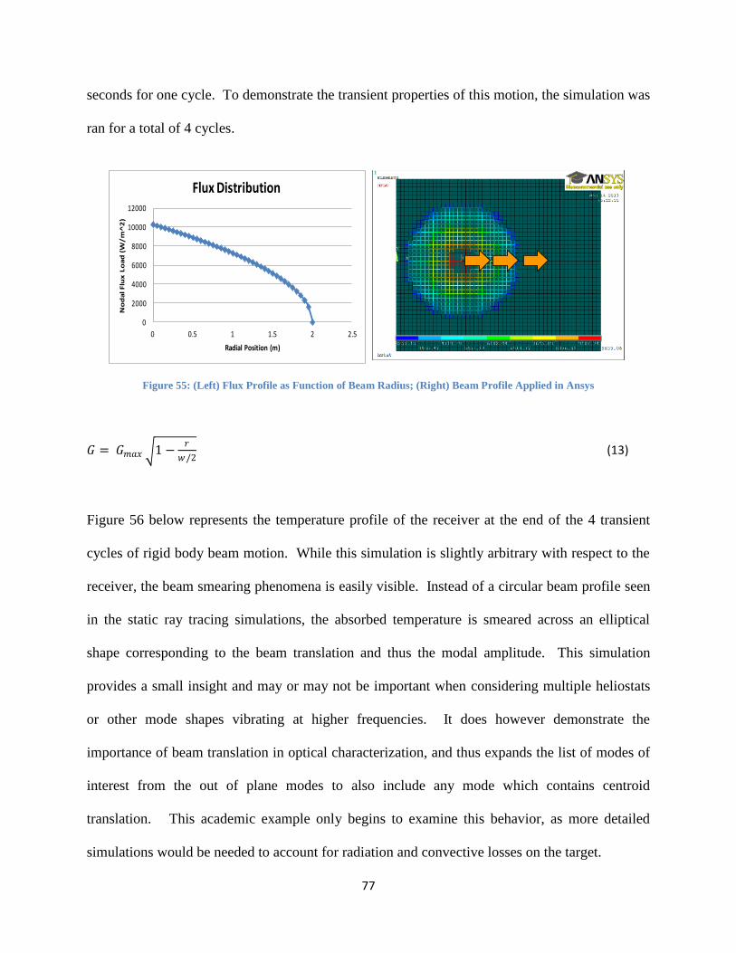
77
seconds for one cycle. To demonstrate the transient properties of this motion, the simulation was
ran for a total of 4 cycles.
Figure 55: (Left) Flux Profile as Function of Beam Radius; (Right) Beam Profile Applied in Ansys
𝐺 = 𝐺𝑚𝑎𝑥 1 −𝑟
𝑤/2 (13)
Figure 56 below represents the temperature profile of the receiver at the end of the 4 transient
cycles of rigid body beam motion. While this simulation is slightly arbitrary with respect to the
receiver, the beam smearing phenomena is easily visible. Instead of a circular beam profile seen
in the static ray tracing simulations, the absorbed temperature is smeared across an elliptical
shape corresponding to the beam translation and thus the modal amplitude. This simulation
provides a small insight and may or may not be important when considering multiple heliostats
or other mode shapes vibrating at higher frequencies. It does however demonstrate the
importance of beam translation in optical characterization, and thus expands the list of modes of
interest from the out of plane modes to also include any mode which contains centroid
translation. This academic example only begins to examine this behavior, as more detailed
simulations would be needed to account for radiation and convective losses on the target.
0
2000
4000
6000
8000
10000
12000
0 0.5 1 1.5 2 2.5
No
da
l F
lux
Lo
ad
(W
/m
^2
)
Radial Position (m)
Flux Distribution

78
Figure 56: Temperature Profile at End of Four Cycles
To further examine the transient behavior of a vibrating beam, some nodal results are compared
for two positions; the center of the target, and one node offset slightly to the edge of the centroid.
Plotted in figures 57-58 are the nodal temperature and absorbed flux for the two positions. This
time dependent simulation results show some cyclic behavior in temperature and flux that
correlate to the natural frequency of the mode shape simulated. Also apparent is a large
difference in magnitude between the centroid and offset nodal results. The offset temperature
starts out the same as the centroid, but the two quickly separate as the beam translates back and
forth. This behavior is explained when examining the frequency of the nodal flux values. The
centroid node position is exposed to the beam centroid nearly twice as fast as the offset node and
corresponds to the natural frequency of the mode. However, the offset node experiences the
beam centroid at a much lower frequency as the beam has a larger distance to travel between
exposures. This interesting result may affect thermal performance over time, however the
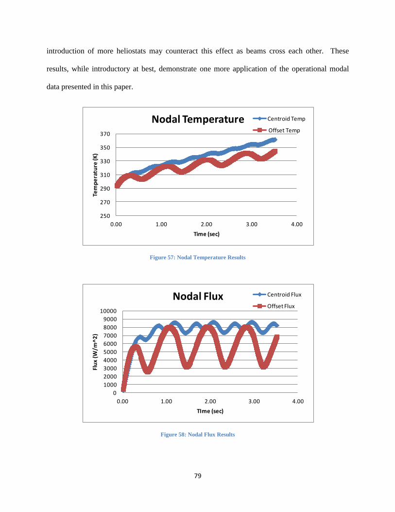
79
introduction of more heliostats may counteract this effect as beams cross each other. These
results, while introductory at best, demonstrate one more application of the operational modal
data presented in this paper.
Figure 57: Nodal Temperature Results
Figure 58: Nodal Flux Results
250
270
290
310
330
350
370
0.00 1.00 2.00 3.00 4.00
Tem
pe
ratu
re (K
)
Time (sec)
Nodal Temperature Centroid Temp
Offset Temp
0
1000
2000
3000
4000
5000
6000
7000
8000
9000
10000
0.00 1.00 2.00 3.00 4.00
Flu
x (W
/m^
2)
TIme (sec)
Nodal Flux Centroid Flux
Offset Flux

80
Future Recommendations & Applications Currently the modal monitoring data acquisition system only streams and logs data with the aid
of a test engineer. The benefit of a in-house developed system built upon the LabVIEW
environment, is the ability to upgrade and modify the system to better reach a new or existing
goal. At the mercy of uncontrollable weather, the ability to automatically monitor wind speed
and trigger data logging based on a user defined threshold will be very helpful in characterizing
wind induced modes. This is only the beginning, as it is possible to further enhance this program
to log different data files for different wind speed bins, time of day, or even remote monitoring
via LabVIEW web applications. Along with this automation, it is also possible to incorporate
real time automated modal identification routines with techniques such as frequency domain
decomposition or FDD. This type of routine was implemented in the early beam data acquisition
example and proved to work quite well for simple cases. One more additional feature that will
prove beneficial is the process of automatic sensor fault detection. As expected with a rotating
structure it is more than likely that sensor wires will become snagged and possible broken over
time. Real time monitoring of correct sensor operation will help to correct this damage as soon
as they occur. These automated procedures will over time provide enough information to verify
early wind excited data and provide a library of data with which to characterize heliostat motion
and wind phenomena such as vortex shedding and turbulence within the field. It will also
provide a base work for future partnerships with existing or new commercial plants wishing to
study this phenomena.
Along with a library of wind excited acceleration data, the system will also provide wind speed,
direction, and strain data at select locations within the field. This data will help verify existing
wind load models and allow for research considering entire array effects as opposed to a single

81
vibrating heliostat. While frontal heliostats are expected to block a majority of incoming wind
speed, the heliostat geometry and mirror spacing provide ideal conditions for vortex shedding
and increased turbulence. From previous wind tunnel research, heliostats were shown to exhibit
higher magnitude vibration with increased turbulence which is most likely the case in a real
heliostat field. This proposes that interior heliostats may actually vibrate as much or more than
exterior heliostats, and future wind monitoring can verify or disprove this theory. Figure 59 is a
screenshot of some initial computational fluid dynamic simulations on the NSTTF heliostat
showing the velocity streamlines of incoming wind on the tilted heliostat and the possibility of
vortex shedding induced modal vibration in adjacent heliostats.
Figure 59: CFD Simulation of NSTTF Heliostat
Current wind load reduction theory originally developed by Peterka et al at NREL suggests that
wind load coefficient are a function of "generalized blockage area" which is the solid area
blocked by upstream heliostats divided by the ground area of that heliostat. This theory allows
for a estimated wind load for interior heliostats and is commonly used in heliostat design. By

82
utilizing the currently instrumented heliostat block, the Peterka wind load model can be verified
over time with future wind excited data collection and aid with CFD model validation. A
primary goal for this research is to inform and develop models that can be used to predict wind
loading in a variety of field configurations, heliostat designs, and wind conditions. Preliminary
CFD model results are inconclusive, but additional refinement and more rigorous computational
simulations are being pursued.
With all this new information, future design criteria based on dynamic heliostat properties can
lead to lower cost and more efficient heliostat designs. With the newly acquired test data, the
FEM of the heliostat can be further calibrated to match all modes of interest and better
approximate rigid body mode translations. With this model, it will then be possible to explore
design modifications with the intent of reducing or completely eliminating the out of plane
modes responsible for the large optical degradations seen in this study. As demonstrated in this
research, the majority of out of plane modes are due to twisting about two un-equal trusses. It is
possible that either extending the shorter truss or connecting the two trusses to further stiffen the
structure and eliminate this motion. By introducing modern vibration control theory to the solar
industry, there is likely many ways to improve structural designs used in renewable energies.
With a validated FEM model, it is possible to explore design modification like these to further
optimize the NSTTF heliostat.
Another current design driving parameter that needs refinement is fatigue prediction in heliostats
and heliostat drive components. High stress areas can lead to premature failure and are currently
calculated using the same analytical models that need full scale validation. With more rigorous
wind modeling and acceleration response data, we can provide a new and more realistic method
of performing these fatigue and life cycle analysis studies. Using real wind speed data at

83
different points in the field along with a validated CFD simulation, it is possible to determine
accurate pressure distributions on the mirror surfaces. Using modern dynamic simulation
packages, analyst can then simulate structurally weak areas and predict failure points in the
NSTTF heliostat. These results will provide as a great benchmark for existing models and
hopefully lead to more efficient heliostat designs.
One final benefit of the unique applications at the NSTTF facility is the long term relationship
with industry partners that wish to test heliostat prototypes at the site. This allows for
collaboration and development of new technologies that actually make its way to commercial
plants. One industry partner has already expressed great interest in dynamic heliostat monitoring
and even assisted with a preliminary modal test on one of their heliostat prototypes located at the
NSTTF. With current large scale plants currently under construction in the southwest, it is
possible to implement this dynamic monitoring experiment in a much larger scale power plant
which will be in constant operation unlike the NSTTF facility. Not only will the optical analysis
presented in this research paper allow for performance improvements, but damage detection can
lead to early repairs which left un-attended could lead to larger, more expensive failures. These
topics demonstrate many areas in CSP research that can benefit from dynamic monitoring, and
will be further explored at Sandia National Laboratories as long as there is a national interest in
CSP technology.
Conclusion Demonstrated in this thesis is just a small introduction to some research topics made possible
thanks to the monitoring system deployed at the National Thermal Test Facility and the
operational results that have been presented here. A custom data acquisition system was
developed to capture wind excited motion within a heliostat field, and has been proven useful in

84
finite element model validation and optical characterization of the NSTTF heliostat. This custom
system provided operational characteristics of a heliostat open to un-disturbed southwestern
winds and will be used to explore entire heliostat array effects with future updates and
operational studies. At this time, the dynamic heliostat project at the NSTTF has provided a set
of validated and scaled mode shapes from the FEM model that are accurate representations of a
exterior heliostat excited by the wind. Using this validated finite element model, a methodology
was developed to approximate the individual performance losses at the instant of modal
excitation for a heliostat at any time or position required. Optical ray tracing simulations were
performed on an ideal day to obtain peak performance metrics for each deformed mode shape
that was output by the FEM. The results from these ray tracing studies verify a suspicion that
modes with predominate motion out of plane with the mirrors lead to the largest reflected flux
loss on the receiver. This loss can be as extreme as a 60% drop in maximum flux for some
modes, and can be used to approximate losses on a larger plant scale. Using the simulation code
DELSOL3, the individual heliostat losses has been applied to an entire field to simulate the
performance drop from a commercial plant perspective. Re-creating the NSTTF heliostat and
plant geometry inside this simulation code, plant performance values were estimated using real
meteorological data. Since the effect of wind speed and magnitude on heliostat excitation is still
unknown for the most part, plant performance loss can be estimated by assuming wind speed
thresholds responsible for mode excitation. This assumption leads to a realistic loss of 2-6% of
electrical power output at the NSTTF depending on wind speed and mode excitation. A
theoretical study was also performed to examine the effect of dynamic losses on plant design
which gives quantitative information regarding the number of heliostats and capital required for
a fictional 100 megawatt plant with the same NSTTF heliostat geometry. The results from this

85
simulation follows the same trend seen regarding out of plane modes, as the drop in power for
these mode shapes requires an additional 660 heliostats and four million dollars to compensate
and ensure the 100 megawatt requirement is met. While the performance results demonstrate a
new cost reduction area with respect to a set of out of plane defined modes, transient thermal
simulation demonstrates beam smearing due to beam translation seen in rigid body modes may
be just as important as modal deformation. This further expands our modes of interest to include
any mode that exhibits this centroid translation which happens to occur at all modes tested. This
is assumed to be a result of the rigid body motion being imposed on all other modes, however
further wind excited analysis is needed to verify realistic displacements.
The modal and optical characterization presented here not only introduces a problem seen in CSP
plant operation, but provides a methodology to test and describe this phenomena. These results
provide an introduction to possible future design criteria desperately needed to drive
concentrating solar power to be competitive in today's renewable energy market. Utilizing the
modal monitoring system developed for this research, industry designers and CSP researchers
alike will have new performance criteria to aid in design and manufacturing. While further wind
excited data is still needed, the simulated operational data introduces the dynamic problem never
before analyzed and provides data sets for future use in engineering studies. With the current
drive to reduce dependence on foreign oil and reduce green house gases, the results presented
here provide a small step forward in moving CSP technology to a new age of competitive
renewable energy technologies.

86
Acknowledgments I would like to take this opportunity to extend my gratitude the a number of colleagues at Sandia
National Laboratories whom aided in this research. Thanks to Cliff Ho for sponsoring this work
and aiding with test planning and funding for modal testing conducted at the NSTTF. I would
also like to thank Todd Griffith and Patrick hunter in the structural dynamics group at Sandia
whom aided in initial testing and analysis. Special thanks to Joshua Christian, Jeremy Sment,
and James Yuan for help with sensor installation and FEM modeling of NSTTF heliostat. I
would also like to extend my gratitude to professor Matt Allen at the University of Wisconsin,
Madison for providing guidance through this research project. Lastly I would like to thank my
friends and family for their continued support and the staff running the Masters Fellowship
Program at Sandia National Labs whom are responsible for the funding and tuition assistance
during this research period.
Sandia National Laboratories is a multi-program laboratory managed and operated by Sandia
Corporation, a wholly owned subsidiary of Lockheed Martin Corporation for the U.S. Department of
Energy’s National Nuclear Security Administration under contract DE-AC04-94AL85000

87
References [1] Kolb, G.J, Ho, C.K, Mancini, T.R, and Gary, J.A, 2011, "Power Tower Technology
Roadmap and Cost Reduction Plan", SAND2011-2419, Sandia National Laboratories,
Albuquerque, NM
[2] Griffith D.T, Ho C.K, Moya, A.C, and Hunter, P.S, "Modal Analysis of a Heliostat for
Concentrating Solar Power", Proceedings of the 30th International Modal Analysis
Conference (IMAC XXX), January 30 – February 2, 2012, Jacksonville, Florida USA.
[3] Griffith, D.T, Moya, A. C, Ho, C, and Hunter, P, “Structural Dynamics Testing and
Analysis for Design Evaluation and Monitoring of Heliostats,” Proceedings of the 5th
ASME International Conference on Energy Sustainability, August 7-10, 2011,
Washington, DC, USA, ESFuelCell2011-54222.
[4] Ho, C.K, Griffith, D.T, Moya, A.C, Sment, J, Christian, J, Yuan, J, and Hunter, P, "
Dynamic Testing and Analysis of Heliostats to Evaluate Impacts of Wind on Optical
Performance and Structural Fatigue", Proceedings of SolarPACES 2012 International
Conference, Marrakech, Morocco, September 11-14, 2012.
[5] Moya, A.C, Griffith D.T, Ho C.K, Sment, J, and Christian, J. "Modal Analysis and
Dynamic Monitoring of a Concentrating Solar Heliostat", Proceedings of the 31st
International Modal Analysis Conference (IMAC XXXI), February, 2013, Orange County,
California.
[6] Peterka, J.A and Derickson, R. G. "Wind Load Design Methods for Ground Based
Heliostats and Parabolic Dish Collectors", Sandia National Laboratories, SAND92-7009,
and Colorado State University 1992
[7] Peterka, J.A, Hosoya, H, N, Bienkiewicz, B, and Cermak, J.E, "Wind Load Reduction for
Heliostats" Solar Energy Research Institute, (DOE Contract DE-AC02-83CH10093)
[8] Gong, B., Z.N. Li, Z.F. Wang, and Y.G. Wang, 2012, "Wind-induced dynamic response
of Heliostat", Renewable Energy, 38(1), p. 206-213.
[9] Wang, Y.G., Z.N. Li, B. Gong, and Q.S. Li, 2009, Wind Pressure and Wind-induced
Vibration of Heliostat, Advances in Concrete and Structures, 400-402, p. 935-940.
[10] Rebolo, R, J. Lata, and J. Vaszuez, "Design of Heliostats Under Extreme and Fatigue
Wind Loads", Proceedings of SolarPACES 2011, Grenada, Spain, September 2012
[11] Pfahl, A, Uhlemann, H. "Wind Loads on Heliostats and Photovoltaic Trackers at Various
Reynolds Numbers", Journal of Wind Engineering and Industrial Aerodynamics, Volume
99, Issue 9, September 2011 (Page 964-968)
[12] Janczy, J. "Modal Analysis of the First Production Design Heliostat Used at the Solar
Thermal Test Facility (STTF)" Vibration & Shock Testing Division 9342, Sandia
National Laboratories (SAND77-1393), September 1977
[13] RE<C Initiative, Google Corporation, http://www.google.org/rec.html Accessed Feb.
2013

88
[14] Moya, A.C and Ho, C.K, “Modeling and Validation of Heliostat Deformation Due to
Static Loading,” Proceedings of 5th ASME International Conference on Energy
Sustainability, August 7-10, 2011, Washington, DC, USA, ESFuelCell2011-54216.
[15] M. S. Allen, “Global and Multi-Input-Multi-Output (MIMO) Extensions of the Algorithm
of Mode Isolation (AMI),” George W. Woodruff School of Mechanical Engineering.
Atlanta, Georgia, Georgia Institute of Technology: 128 pages, 2005.
[16] Miles, John W. "On Structural Fatigue Under Random Loading", Journal of Aeronautical
Sciences (Page 753), November 1954
[17] Simmons, Ryan. "Basics of Miles Equation", FEMCI (Finite Element Modeling
Continuous Improvement) Book, NASA Goddard Space Flight Center, May 2001
[18] Mercer, C. "Acceleration, Velocity, and Displacement Spectra - Omega Arithmetic"
Technical Director, ProSIG Signal Processing Tutorials
[19] Christian, J.M., Ho, C.K., "Finite Element Modeling of Concentrated Solar Collectors for
Evaluation of Gravity Loads, Bending, and Optical Characterization," Proceedings of the
4th ASME International Conference on Energy Sustainability, May 17-22, 2010,
Phoenix, Arizona, USA, ES2010-90050
[20] Kistler, B. L., "A User's Manual for DELSOL3: A Computer Code for Calculating the
Optical Performance and Optimal System Design for Solar Thermal Central Receiver
Plants", Sandia Report (SAND86-8018), November 1986
[21] Typical Meteorological Year Data Provided by Renewable Resource Data Center, NREL
(National Renewable Energy Department http://www.nrel.gov/rredc/, accessed Jan. 2013

89
Appendix
A: Ansys and OMA Mode Shape Plots
-1000
100200 -150
-100-50
050
100150
0
50
100
150
200
250
300
HZ
Natural Frequency (Hz):0.88316
HX
HY
-100-50050100150200250
-100
0
100
0
50
100
150
200
250
300
HZ
Natural Frequency (Hz):1.6386
HX
HY
-100-500501001502002500
50
100
150
200
250
300
HX
Natural Frequency (Hz):3.2418
HY

90
-100
-50
0
50
100
150
200
250
-150-100
-500
50100
150
0
100
200
300
HZ
Natural Frequency (Hz):2.2476
HX
HY
-100
0
100
200-150
-100
-50
0
50
100
150
0
100
200
300
HZ
Natural Frequency (Hz):3.2418
HX
HY
-100
0
100
200-150
-100-50
050
100150
0
50
100
150
200
250
300
HZ
Natural Frequency (Hz):4.0262
HX
HY
-100
0
100
200
-150
-100
-50
0
50
100
150
0
100
200
300
HZ
Natural Frequency (Hz):4.1273
HX
HY

91
-100
0
100
200-100
0
100
0
50
100
150
200
250
300
HZ
Natural Frequency (Hz):4.1273
HX
HY

92
-100-50050100150200250
-100
0
100
0
50
100
150
200
250
300
HZ
Natural Frequency (Hz):4.4961
HX
HY
-1000
100200
-150-100
-500
50100
1500
50
100
150
200
250
300
HZ
Natural Frequency (Hz):4.6583
HX
HY
-100
0
100
200 -150-100
-500
50100
150
0
100
200
300
HZ
Natural Frequency (Hz):4.1263
HX
HY

93
-100
0
100
200-150
-100-50
050
100150
0
50
100
150
200
250
300
HZ
Natural Frequency (Hz):5.6109; Damping = 0.0020671
HX
HY
-100
0
100
200 -150-100
-500
50100
150
0
100
200
300
HZ
Natural Frequency (Hz):6.0312; Damping = 0.0017282
HX
HY
-100
0
100
200-150
-100-50
050
100150
0
50
100
150
200
250
300
HZ
Natural Frequency (Hz):6.6352; Damping = 0.0012917
HX
HY

94
-100-50
050
100150
200250
-100
0
100
0
50
100
150
200
250
300
HZ
Natural Frequency (Hz):7.1018; Damping = 0.0016398
HX
HY
-100
0
100
200
-150
-100
-50
0
50
100
150
0
100
200
300
HZ
Natural Frequency (Hz):8.6147; Damping = 0.00061799
HX
HY
-100
0
100
200
-150
-100
-50
0
50
100
150
0
100
200
300
HZ
Natural Frequency (Hz):9.019; Damping = 0.00092677
HX
HY

95
-100
0
100
200 -100
0
100
0
50
100
150
200
250
300
HZ
Natural Frequency (Hz):9.3762; Damping = 0.00055748
HX
HY

96
-100
0
100
200
-100
0
100
0
50
100
150
200
250
300
HZ
Natural Frequency (Hz):9.7025; Damping = 0.00025857
HX
HY
-100-50
050
100150
200250
-100
0
100
0
50
100
150
200
250
300
HZ
Natural Frequency (Hz):10.1504; Damping = 0.00064538
HX
HY

97
B: Miles Approximate Displacements per Mode
0 5 10 15 20 250
0.005
0.01
0.015
0.02
0.025
0.03
DOF #
Dis
pla
cem
ent
(m)
Recovered Miles RMS Displacement wn = 0.873Hz
Max Steady Disp = 0.026548 m
0 5 10 15 20 250
1
2
3
4
5
6
7x 10
-3
DOF #
Dis
pla
cem
ent
(m)
Recovered Miles RMS Displacement wn = 1.6577Hz
Max Steady Disp = 0.0065985 m
0 5 10 15 20 250
1
2
3
4
5
6
7
8x 10
-4
DOF #
Dis
pla
cem
ent
(m)
Recovered Miles RMS Displacement wn = 3.1125Hz
Max Steady Disp = 0.00078205 m
0 5 10 15 20 250
0.1
0.2
0.3
0.4
0.5
0.6
0.7
0.8
0.9
1x 10
-3
DOF #
Dis
pla
cem
ent
(m)
Recovered Miles RMS Displacement wn = 2.2307Hz
Max Steady Disp = 0.00096751 m
0 5 10 15 20 250
0.5
1
1.5
2
2.5
3
3.5
4x 10
-3
DOF #
Dis
pla
cem
ent
(m)
Recovered Miles RMS Displacement wn = 3.2418Hz
Max Steady Disp = 0.0036342 m
0 5 10 15 20 250
1
2
x 10-4
DOF #
Dis
pla
cem
ent
(m)
Recovered Miles RMS Displacement wn = 4.0358Hz
Max Steady Disp = 0.00020659 m

98
0 5 10 15 20 250
0.5
1
1.5
2
2.5
3
3.5
4
4.5
5x 10
-3
DOF #
Dis
pla
cem
ent
(m)
Recovered Miles RMS Displacement wn = 4.1263Hz
Max Steady Disp = 0.0047754 m
0 5 10 15 20 250
1
2
x 10-4
DOF #
Dis
pla
cem
ent
(m)
Recovered Miles RMS Displacement wn = 4.4978Hz
Max Steady Disp = 0.00022329 m
0 5 10 15 20 250
0.5
1
1.5
2
2.5
3
3.5x 10
-4
DOF #
Dis
pla
cem
ent
(m)
Recovered Miles RMS Displacement wn = 4.6756Hz
Max Steady Disp = 0.00034354 m
0 5 10 15 20 250
1
2
3
4
5
6x 10
-3
DOF #
Dis
pla
cem
ent
(m)
Recovered Miles RMS Displacement wn = 4.1257Hz
Max Steady Disp = 0.0051704 m
0 5 10 15 20 250
1
2
x 10-4
DOF #
Dis
pla
cem
ent
(m)
Recovered Miles RMS Displacement wn = 5.6144Hz
Max Steady Disp = 0.00029933 m
0 5 10 15 20 250
0.5
1
1.5
2
2.5
3
3.5
4
4.5x 10
-4
DOF #
Dis
pla
cem
ent
(m)
Recovered Miles RMS Displacement wn = 6.0349Hz
Max Steady Disp = 0.00041149 m

99
0 5 10 15 20 250
0.2
0.4
0.6
0.8
1
1.2x 10
-3
DOF #
Dis
pla
cem
ent
(m)
Recovered Miles RMS Displacement wn = 6.645Hz
Max Steady Disp = 0.0011298 m
0 5 10 15 20 250
1
2
3
4
5
6x 10
-4
DOF #
Dis
pla
cem
ent
(m)
Recovered Miles RMS Displacement wn = 7.1064Hz
Max Steady Disp = 0.0004782 m
0 5 10 15 20 250
1
2
3
4
5
6x 10
-4
DOF #
Dis
pla
cem
ent
(m)
Recovered Miles RMS Displacement wn = 8.6221Hz
Max Steady Disp = 0.00054536 m
0 5 10 15 20 250
1
2
3
4
5
6x 10
-4
DOF #
Dis
pla
cem
ent
(m)
Recovered Miles RMS Displacement wn = 9.019Hz
Max Steady Disp = 0.000581 m
0 5 10 15 20 250
0.2
0.4
0.6
0.8
1
1.2x 10
-3
DOF #
Dis
pla
cem
ent
(m)
Recovered Miles RMS Displacement wn = 9.3972Hz
Max Steady Disp = 0.0010078 m
0 5 10 15 20 250
0.2
0.4
0.6
0.8
1
1.2
1.4x 10
-3
DOF #
Dis
pla
cem
ent
(m)
Recovered Miles RMS Displacement wn = 9.3752Hz
Max Steady Disp = 0.0030307 m

100
0 5 10 15 20 251.2
1.4
1.6
1.8
2
2.2
2.4x 10
-4
DOF #
Dis
pla
cem
ent
(m)
Recovered RMS Displacement wn = 9.7025Hz
Max Steady Disp = 0.0002356 m
0 5 10 15 20 250.8
0.9
1
1.1
1.2
1.3
1.4
1.5
1.6x 10
-4
DOF #
Dis
pla
cem
ent
(m)
Recovered RMS Displacement wn = 10.1504Hz
Max Steady Disp = 0.00015856 m

101
C: APEX Ray Tracing Results

102

103

104

105

106

107

108

109

110
111

112