mod functions: a new approach to function theory
DESCRIPTION
In this book the notion of MOD functions are defined on MOD planes. This new concept of MOD functions behaves in a very different way. Even very simple functions like y = nx has several zeros in MOD planes where as they are nice single line graphs with only (0, 0) as the only zero. Further polynomials in MOD planes do not in general follows the usual or classical laws of differentiation or integration.TRANSCRIPT


MOD Functions: A New Approach
to Function Theory
W. B. Vasantha Kandasamy Ilanthenral K
Florentin Smarandache
2015

2
This book can be ordered from:
EuropaNova ASBL
Clos du Parnasse, 3E
1000, Bruxelles
Belgium
E-mail: [email protected]
URL: http://www.europanova.be/
Copyright 2014 by EuropaNova ASBL and the Authors
Peer reviewers:
Prof. Gabriel Tica, Bailesti College, Bailesti, Jud. Dolj, Romania.
Dr. Stefan Vladutescu, University of Craiova, Romania.
Dr. Octavian Cira, Aurel Vlaicu University of Arad, Romania.
Said Broumi, University of Hassan II Mohammedia,
Hay El Baraka Ben M'sik, Casablanca B. P. 7951.
Morocco.
Many books can be downloaded from the following
Digital Library of Science:
http://www.gallup.unm.edu/eBooks-otherformats.htm
ISBN-13: 978-1-59973-364-7
EAN: 9781599733647
Printed in the United States of America

3
CONTENTS
Preface 5
Chapter One
SPECIAL TYPE OF DECIMAL POLYNOMIALS 7 Chapter Two
MOD POLYNOMIAL FUNCTIONS 11
Chapter Three
MOD COMPLEX FUNCTIONS
IN THE MOD COMPLEX PLANE CN(M) 113

4
Chapter Four
TRIGONOMETRIC, LOGARITHMIC
AND EXPONENTIAL MOD FUNCTIONS 131
Chapter Five
NEUTROSOPHIC MOD FUNCTIONS
AND OTHER MOD FUNCTIONS 163
Chapter Six
SUGGESTED PROBLEMS 187
FURTHER READING 199
INDEX 202
ABOUT THE AUTHORS 203

5
PREFACE
In this book the notion of MOD functions are defined on
MOD planes. This new concept of MOD functions behaves in a
very different way. Even very simple functions like y = nx has
several zeros in MOD planes where as they are nice single line
graphs with only (0, 0) as the only zero.
Further polynomials in MOD planes do not in general
follows the usual or classical laws of differentiation or
integration.
Even finding roots of MOD polynomials happens to be very
difficult as they do not follow the fundamental theorem of
algebra, viz a nth degree polynomial p(x) in MOD plane or MOD
intervals do not have n roots for + and × are defined on them, do
not satisfy the distributive laws.

6
These drawbacks becomes a challenging issue. So study in
this direction is open. In fact several open conjectures are
proposed in this book. However this paradigm of shift will give
new dimension to mathematics.
We wish to acknowledge Dr. K Kandasamy for his
sustained support and encouragement in the writing of this
book.
W.B.VASANTHA KANDASAMY
ILANTHENRAL K
FLORENTIN SMARANDACHE

Chapter One
SPECIAL TYPE OF DECIMAL
POLYNOMIALS In this chapter we define several special types of decimal
polynomials. The motivation for constructing decimal
polynomials is that while doing integration or differentiation the
power of x in the polynomial p(x) is either increased by 1 or
decreased by 1 respectively.
We want to increase or decrease to any value inbetween 0
and 1. For this we have built decimal polynomial rings.
Further using these decimal polynomial rings we will be in
a position to define, describe and develop the notion of MOD
calculus.
DEFINITION 1.1: Let R[x0.1
] be the decimal polynomial ring
generated by the decimal power of x0.1
.
R[x0.1
] = 0.1
∞
=
∑ i
i
i
a x ai are reals}.
Clearly R[x0.1
] is a ring for we see for any p(x0.1
) and q(x0.1
)
in R[x0.1
]; p(x0.1
) + q(x0.1
) ∈ R[x0.1
].

8 MOD Functions
For instance if
p(x0.1
) = 3x0.3
+ 4.7x0.6
+ 8.3x0.9
– 13.7x8 + 3
and
q(x0.1
) = 7x0.1
– 9x0.6
+ 14.7x0.9
– 3x8 – 10 ∈ R[x
0.1]
then
p(x0.1
) + q(x0.1
) = –7 + 7x0.1
+ 3x0.3
– 4.3x0.6
+ 23x0.9
– 16.7x8 ∈ R[x
0.1].
This is the way addition operation is performed on R[x0.1
].
We see if
p(x0.1
) = 3 – 2x0.3
+ 7x6.3
and
q(x0.1
) = 2 + 4x0.5
+ 10x0.7
∈ R[x0.1
]
then
p(x0.1
) × q(x0.1
) = (3 – 2x0.3
+ 7x6.3
) (2 + 4x0.5
+ 10x0.7
)
= 6 – 4x0.3
+ 14x6.3
+ 12x0.5
– 8x0.8
+ 28x6.8
+ 30x0.7
– 20x + 70x7 ∈ R[x
0.1].
This is the way + and × operation are performed. It can be
easily verified R[x0.1
] is a commutative ring of infinite order.
Now a natural question would be how to solve equations in
R[x0.1
].
The easiest way is R[x0.1
] can be mapped isomorphically on
to R[x] by the map η : R[x0.1
] → R[x]
(or η : R[x] → R[x0.1
])
by η (r) = r if r ∈ R
η(x0.1
) = x (or η(r) = r for all r ∈ R and η(x) = x0.1
)
η(x42
) = x4.2
and η(x3) = x
0.3.

Special Type of Decimal Polynomial 9
So if p(x) = x2 – 4x + 4 ∈ R[x], then
p(x0.1
) = x0.2
– 4x0.1
+ 4.
So solving p(x) is easy and from which we conclude the
roots of p(x0.1
) are x0.1
= 2, 2.
On similar lines we can further lessen the power of x and
define R[x0.01
]; this will also be a ring.
Clearly R[x] ⊆ R[x0.1
] ⊆ R[x0.01
].
R[x0.01
] is also a decimal polynomial ring generated by x0.01
.
We call these decimal polynomial rings as MOD
polynomials or very small polynomials with real coefficients [5-
10].
However we want to keep the power of x as x0.1
or x0.01
or
x0.001
or x0.0001
and so on. This is the condition we impose for
some easy working.
For η : R[x0.001
] → R[x] is obtained by dividing/multiplying
the power of x by thousand.
Likewise η : R[x] → R[x0.001
] is got by dividing the power
of x by 1000.
So η can also be realized as the homomorphism of a special
type.
We make one special condition for the sake of
complatability; we by no means take powers of x0.1
as decimal
powers; that is ( )n
0.1x , where n is always assumed to be a
positive integer greater than or equal to 1.

10 MOD Functions
So we have to take ( )0.7
0.1x or any such sort. As far as
possible we in this book define only; ( )m
0.1x = x0.m
(m < 10)
where m is an integer
( )8
0.1x = x0.8
,
( )21
0.1x = x2.1
,
( )125
0.1x = x12.5
and so on.
Likewise for x0.01
also we do not raise to a fractional power
of x0.01
. ( )n
0.1x is defined if and only if n ∈ N.
Under these conditions and constraints only we work, that is
why we call it as MOD polynomial real rings.
Study of MOD polynomial real rings can be done as a matter
of routine.
Now we define MOD polynomial complex rings C[x0.1
],
C[x0.01
] and C[x0.001
] and so on.
We as in case of reals work with complex MOD
polynomials.
Next we proceed onto describe MOD modulo integer
polynomials Zn[x0.1
], Zn[x0.01
], Zn[x0.001
] and so on.
We can also have MOD interval modulo integer
polynomials.
[0, m)[x0.1
], [0, m)[x0.01
], [0, m)[x0.001
] and so on.
We will be using these MOD polynomial rings to build the
MOD calculus.

Chapter Two
MOD POLYNOMIAL FUNCTIONS
The concept of MOD planes was introduced in [24]. Here we
discuss about the MOD polynomial functions. Let [0, m) be the
MOD interval (m ≥ 2).
p (x) ∈ [0, m)[x] = i
i
i 0
a x∞
=
∑ ai ∈ [0, m)} is defined as the
MOD polynomials.
y = f (x) is called the MOD polynomial function in the
independent variable x and y = f (x) is defined in the MOD real
plane Rn (m).
The following facts are innovative and important.
(i) A polynomial defined over the MOD plane is
continuous or otherwise depending on m of Rn (m).
(ii) For the same p (x) we have various types of
associated graphs depending on Rn (m).
(iii) p (x) has infinite number of properties in contrast to
p (x) ∈ R[x] which is unique. This flexibility is
enjoyed by MOD polynomial function which makes
it not only interesting but useful in appropriate
applications.
We will illustrate this situation by some examples.

12 MOD Functions
Example 2.1: Let p (x) = x + 4 ∈ R[x] (R reals). The graph of x
+ 4 is as follows:
-6 -5 -4 -3 -2 -1 1 2 3 4 5 6 7 8 9 10
-2
-1
1
2
3
4
5
6
7
8
9
10
11
12
13
14
x
y
Figure 2.1
Clearly the function y = x + 4 is a continuous curve.
Now y = x + 4 is transformed into the MOD plane Rn(2) as
y = x. The graph of y = x in the MOD plane Rn(2) is given in
Figure 2.2.
Clearly the graph of y = x + 4 where the function is
transformed as y = x is again a continuous curve.
Now let us find the curve of y = 4 + x in the MOD plane
Rn(3). The function y = x + 4 is transformed to y = x+1 in the
MOD plane Rn(3). The graph of y = x + 1 is given in Figure 2.3.
Clearly the function y = x + 1 is not a continuous function
in the MOD plane Rn(3).

MOD Polynomial Functions 13
0 0.5 1 1.5 2
0.5
1
1.5
2
X
Y
Figure 2.2
0 0.5 1 1.5 2 2.5 30
0.5
1
1.5
2
2.5
3
X
Y
Figure 2.3

14 MOD Functions
In fact two pieces of continues curves in the intervals [0, 2)
and [2, 3).
Thus the function y = x + 1 is continuous in the interval
[0, 2) then it is again continuous in the interval [2, 3).
At x = 2, y = 0. Thus the function increases from 1 to 1.999
in the interval [0, 2) and drops to 0 at x = 2 and again increases
from 0 to 0.9999 …, in the interval [2, 3).
Next we consider the function y = x + 4 in the MOD plane
Rn(4). The graph of y = x in Rn(4) is given in Figure 2.4.
0 0.5 1 1.5 2 2.5 3 3.5 4
0.5
1
1.5
2
2.5
3
3.5
4
X
Y
Figure 2.4
We see in case of the MOD plane Rn(4); y = x + 4 that is
y = x is a straight line similar to the function in the MOD plane
Rn(2). The function is continuous in Rn(4).

MOD Polynomial Functions 15
Now we study the function y = x + 4 in the MOD plane
Rn(5). The associated graph is given in Figure 2.5.
0 1 2 3 4 5
1
2
3
4
5
x
y
Figure 2.5
We see again the function y = x + 4 is not a continuous
curve in Rn(5). The function is continuous in [0, 1) and at 1 it
drops to 0 and again y = x + 4 is continuous from [1, 5).
Thus the function is an increasing function in [0, 1) at
1 drops to 0 and again increasing in the interval [1, 5).
Now we define the function y = x + 4 in the MOD plane
Rn(6).
The graph of the function in the MOD plane Rn(6) is given in
Figure 2.6.
The function y = x + 4 is increasing in the interval [0, 2) and
is continuous.
Further the function y = x + 4 is continuous in the interval
[2, 6) and drops to 0 at x = 2.

16 MOD Functions
0 1 2 3 4 5 6
1
2
3
4
5
6
x
y
Figure 2.6
Consider the function y = x + 4 in the MOD plane Rn(7). The
graph of the function y = x + 4 is given in Figure 2.7.
0 1 2 3 4 5 6 7
1
2
3
4
5
6
7
x
y
Figure 2.7

MOD Polynomial Functions 17
Here also the function is not continuous. At x = 3 it drops to
zero. The function is increasing in the interval [0, 3) and drops
to zero at 3 and increasing in the interval [3, 7).
The range values are [4, 7) and [0, 4).
Now we see the graph of the function y = x + 4 in the MOD
plane Rn(8).
The graph of the function y = x + 4 in the MOD plane Rn(8)
is as given as Figure 2.8.
0 1 2 3 4 5 6 7 8
1
2
3
4
5
6
7
8
x
y
Figure 2.8
The function increases from 4 to 7.999 and drops to zero at
x = 4 and again increases from 0 to 3.999.
Thus we see the function y = x + 4 in the MOD plane Rn (m)
(m ≥ 4) is as follows:

18 MOD Functions
y = x + 4 increases in the interval [0, m–4) and drops at
m – 4 to zero and again increases from [m–4, m).
The graph of y = x + 4 in the MOD plane Rn (m) is as
follows:
Figure 2.9
Example 2.2: Next we study the function y = x2 + 1 in the real
plane and then the graph of the function y = x2 + 1 in the MOD
plane Rn (m). The graph of y = x2 + 1 in the real plane R is
given in Figure 2.10.
The function is a continuous curve.
Now we study the function yn = x2 + 1 in the MOD plane
Rn(2). At x1 = 1 yn = 0, at x2 = 1.7320508076 y = 0. The
associated graph is given in Figure 2.11.

MOD Polynomial Functions 19
-7 -6 -5 -4 -3 -2 -1 1 2 3 4 5 6 7 8 9 10
1
2
3
4
5
6
7
8
9
10
11
12
13
14
15
x
y
Figure 2.10
0 0.5 1 1.5 2
0.5
1
1.5
2
X
Y
Figure 2.11

20 MOD Functions
The function is not a continuous graph.
The function is continuous in the interval [0, 1),
[1, 1.7320508074) and [1.7320508076, 2) and at x1 and x2 drops
to zero.
Next we study the function y = x2 + 1 in the MOD plane
Rn(3).
0 0.5 1 1.5 2 2.5 30
0.5
1
1.5
2
2.5
3
X
Y
Figure 2.12
At x1 = 1.4142135625, y = 0 in Rn(3).
At x2 = 2.2360679776, y = 0
At x3 = 2.8284271248, y = 0
Thus yn = x2 + 1 in Rn(3) has three zeros given by x1, x2 and
x3 we see yn = x2 + 1 in Rn(2) also has only three zeros.
The function is continuous at [0.1, 1.4142135625…) and
[1.4142135625, 3) drops to zero at, 1.4142135625.

MOD Polynomial Functions 21
At x = 2.2360679776, y = 0.
At x = 2.8284271248, y = 0.
Next we study the MOD function y = x2 + 1 on the MOD
plane Rn(4). The graph of the function is as follows:
0.5 1 1.5 2 2.5 3 3.5 40
0.5
1
1.5
2
2.5
3
3.5
4
X
Y
Figure 2.13
At x = 1.7320508076, y = 0.
At x = 2.645751311, y = 0.
At x = 3.31662479, y = 0.
Thus when y = x2 + 1 is the function defined on Rn (m)
m ≥ 2.
The graph of the function in the plane Rn (m).

22 MOD Functions
Figure 2.14
where for some t = s.9…. The function drops to zero.
The graph is not continuous has several branches and each
branch is continuous in the interval [0, t…).
It is left as an open conjecture to find the zeros of y = x2 + 1
in Rn (m).
(i) m prime.
(ii) m odd.
(iii) m even.
Example 2.3: Let us consider the function y = x3 + 1 in the real
plane and the MOD real planes Rn (m); m ≥ 2. The associated
graph is given in Figure 2.15.
Now we consider the same function y = x3 + 1 in the MOD
plane Rn(2) which is given in Figure 2.16.

MOD Polynomial Functions 23
-7 -6 -5 -4 -3 -2 -1 1 2 3 4 5 6 7 8 9
-7
-6
-5
-4
-3
-2
-1
1
2
3
4
5
6
7
8
9
x
y
Figure 2.15
0 0.5 1 1.5 2
0.5
1
1.5
2
X
Y
Figure 2.16

24 MOD Functions
y = x3 + 1 representation in the MOD plane Rn(2).
The graph is not continuous, it is continuous and increasing
in the interval [0, 1) and drops to zero at x = 1 and steady
increases up to y = 1 in the interval [1, 2).
Next we study the function y = x3 + 1 in Rn(3).
For x1 = 1.2599210498 the y value is zero.
There is a zero lying between 1.7 and 1.71.
At x2 = 1.7099759467, y = 0.
At x3 = 2, y = 0
Now at
x4 = 2.2239800909, y = 0.
When
x5 = 2.410142264 we get y = 0.
When
x6 = 2.5712815908; y = 0.
At x7 = 2.7144176164 we get y = 0.
At x8 = 2.84386698 we get y = 0.
At x9 = 2.9624960684; y = 0.
Thus yn = x3 + 1 is not continuous and it has 9 zeros and
there are 10 discontinuous curves.
Given by the Figure 2.17.
(x1)3 + 1 = 3 (mod 3) = 0,
(x2)3 + 1 = 6 (mod 3) = 0,
(x3)3 + 1 = 9 (mod 3) = 0,
(x4)3 + 1 = 12 (mod 3) = 0,
(x5)3 + 1 = 15 (mod 3) = 0,

MOD Polynomial Functions 25
0 0.5 1 1.5 2 2.5 30
0.5
1
1.5
2
2.5
3
X
Y
Figure 2.17
(x6)3 + 1 = 18 (mod 3) = 0,
(x7)3 + 1 = 21 (mod 3) = 0,
(x8)3 + 1 = 24 (mod 3) = 0 and
(x9)3 + 1 = 27 (mod 3) = 0.
Thus it is conjectured if yn = xp + 1 in the MOD plane Rn (p);
p a prime; will yn = xp + 1 have p
2 number of zeros says x1, …,
2px with (x1)
p + 1 = p (mod p) = 0 and so on.
y = 0 occurs when x ∈ (1.2, 1.3) and the function is
increasing upto x = 1.7, y = 2.913.
When x = 2.8, y = 2.952 when x = 2.9, y = 1.38.
The pattern of the function y = x3 + 1 in the MOD plane
Rn(3) needs more investigation, thus the above figure gives
most of the branches of the curve in the MOD plane Rn(3).
Now we consider the function y = x3 + 1 in the MOD plane
Rn(4).

26 MOD Functions
0.5 1 1.5 2 2.5 3 3.5 40
0.5
1
1.5
2
2.5
3
3.5
4
X
Y
Figure 2.18
when x = 1.4 y = 3.744
when x = 1.42 y = 3.862
when x = 1.44 y = 3.985
when x = 1.49 y = 0.3079
when x = 1.48 y = 0.241792
when x = 1.46 y = 0.112136
when x = 1.45 y = 0.048625
So y = 0 for a point in the interval x = 1.44 and x = 1.45
When x = 1.448 y = 0.0360
When x = 1.445 y = 0.017196
When x = 1.446 y = 0.0234
When x = 1.444 y = 0.0109
When x = 1.443 y = 0.004685307
x = 1.4425 y = 0.0015
x = 1.4422 y = 3.9995

MOD Polynomial Functions 27
when x = 1.4423 y = 0.000315
when x = 1.44225 y = 0.0000027
when x = 1.442249 y = 3.9999964
when x = 1.4422499 y = 0.00000206
when x = 1.4422496 y = 0.000000185
when x = 1.44224958 y = 0.00000006
when x = 1.442249575 y = 0.000000029.
Thus y = 0 for a value of x in the interval
(1.442249575, 1.44224958)
The graph of the curve needs study for the graph is
discontinuous.
Finding the number of branches of y = x3 + 1 in Rn(4) is left
as an exercise to the reader.
Finally we study the graph of y = x3 + 1 in the MOD plane
Rn(5).
0 1 2 3 4 5
1
2
3
4
5
x
y
Figure 2.19
y = 0 at a point between 2.41 and 2.42.

28 MOD Functions
Thus we get some four bits of the curve for the MOD
equation y = x3 + 1 in the MOD plane Rn(5) [x].
However finding all the braches of the MOD equation
y = x3 + 1 in Rn(5) is left as an exercise to the reader.
Now we study the same function y = x3 + 1 in the MOD
plane Rn(6).
1 2 3 4 5 60
1
2
3
4
5
6
x
y
Figure 2.20
y = 0 for some x = (2.5, 2.6). For x = 3.05 we get y = 5.37 y
= 0 for some x ∈ (3.07, 3.08).
For y = 0 for some x ∈ (4.02, 4.03).
This happens to be a open conjecture to study the number of
zeros of x3 + 1 ∈ Rn (m); m = 2, 3, 4, …, m (m < ∞).
Thus when y = x3 + 1 is the function defined on Rn (m),
m ≥ 2. The graph of the function in the plane Rn (m).

MOD Polynomial Functions 29
Figure 2.21
where for some t = s.9… The function drops to zero. The graph
is not continuous one has to find all the branches are continuous
in the interval [0, t…) and at t.9 drops to zero and again the
function is a continuous increasing function in [t…m).
Even a simple function x3 + 1 = y which remains as it is in
every MOD plane after transformation has very many different
forms and none of them are continuous in the MOD plane.
Further it is another open conjecture to study how many bits
of curves the function y = x3 + 1 will be represented in the MOD
plane Rn (m).
We mean by bits the number of continuous branches of the
graph. Thus it is again dependent on the number of zeros a
function y = x3 + 1 has in Rn (m)[x].

30 MOD Functions
This function y = x3 + 1 is defined as the unchangable
universal function as y = x3 + 1 ∈ R[x] remains the same on
every MOD plane Rn (m)[x].
DEFINITION 2.1: A function y = f (x) ∈ R[x] which remains the
same over Rn (m)[x] for every 2 ≤ m < ∞ is defined as the
unchangeable universal MOD function.
We will give examples of them.
Example 2.4: Let y = x2 + 1, x
3 + 1, x
5 + 1, x
4 + 1, …, x
t + 1 + 1,
(2 ≤ t < ∞), x2 + x + 1, x
3 + x + 1, x
3 + x
2 + 1 and so on.
xt + x
t–1 + … + 1, x
t + 1t rx − + … + 1, 0 < r1 < t are all
unchangeable universal MOD functions.
DEFINITION 2.2: Let y = f (x) ∈ R[x]. If y = f (x) changes
depending on Rn (m)[x] then we define y = f (x) as a changeable
universal MOD functions.
We will give examples of them.
Example 2.5: Let y = x7 + 9x + 1 ∈ R[x] be the function. This is
a changeable universal function in the MOD polynomial Rn
(m)[x]. However for m ≥ 10 this function f (x) = x7 + 9x + 1
remains unchangeable. But for all 2 ≤ m ≤ 9 the function is a
changeable function. y = x7 + 9x + 1 = x
7 + x + 1 in Rn(2).
y = x7 + 9x + 1 = x
7 + 1 in Rn(3),
x7 + 9x + 1 = x
7 + x + 1 in Rn(4),
x7 + 9x + 1 = x
7 + 4x + 1 in Rn(5),
x7 + 9x + 1 = x
7 + 3x + 1 in Rn(6),
x7 + 9x + 1 = x
7 + 2x + 1 in Rn(7),

MOD Polynomial Functions 31
x7 + 9x + 1 = x
7 + x + 1 in Rn(8) and
x7 + 9x + 1 = x
7 + 1 in Rn(9).
Thus this function is a changeable one for m ≤ 9.
Next we give an example with graphs.
Example 2.6: Let y = x2 + 9x + 1 ∈ R[x]. Now
y = x2 + 9x + 1 = x
2 + x + 1 ∈ Rn(2)[x].
We just describe the graph of them. The graph of y = x2 + x
+ 1 in the plane Rn(2).
0 0.5 1 1.5 2
0.5
1
1.5
2
X
Y
Figure 2.22
y = 0 for x ∈ (0.6, 0.7)
y = 0 for x ∈ (1.3, 1.4)

32 MOD Functions
For
x = 1.79 y = 1.99; y = 0 for x ∈ (1.79, 1.799)
For
x = 1.98 y = 0.9004.
So four bits of curves and the function attain zero in three
points mentioned above.
Let y = x2 + 9x + 1 ∈ R[x] this function in Rn(3) is
y = x2 + 1.
The graph of x2 + 1 in the MOD plane Rn(3) is as follows:
0 0.5 1 1.5 2 2.5 30
0.5
1
1.5
2
2.5
3
X
Y
Figure 2.23
y = 2.9881 for x = 1.41 for x = 1.415 y = 0.002225 so for
some x ∈ (1.41, 1.415); y = 0.
For x = 2.23 y = 2.9729

MOD Polynomial Functions 33
For x = 2.24 y = 0.0176
For x = 2.25 y = 0.0625.
Thus for some x ∈ (2.23, 2.24) y = 0.
For x = 2.9 y = 0.41. For x = 2.99; y = 0.9401.
Thus we get the above graph which has only two zero.
Next we consider the function y = x2 + 9x + 1 ∈ R[x] in the
MOD plane Rn(4).
The graph y = x2 + x + 1 in the MOD plane Rn(4) is as
follows:
0.5 1 1.5 2 2.5 3 3.5 40
0.5
1
1.5
2
2.5
3
3.5
4
X
Y
Figure 2.24

34 MOD Functions
When x= 1.3, y = 3.99.
When x = 1.5, y = 0.75
x = 1.4, y = 0.36
x = 1.35, y = 0.1725
x = 1.31, y = 0.026
For some x ∈ (1.3, 1.31) there a y such that y = 0.
For x = 2.1, y = 3.51
For some x ∈ (2.18, 2.2), y = 0.
For x = 3.4 y = 3.96
For x = 3.402 y = 3.97
For x = 3.405 y = 3.999
For x = 3.45 y = 0.3525
Thus for some x ∈ (3.405, 3.41), y = 0.
For x = 3.9; y = 0.11
For x = 3.99, y = 0.9101.
Thus x2 + x + 1 has three zeros in the MOD plane Rn(4).
Now the function y = x2 + 9x + 1 in the MOD plane Rn(5) is
y = x2 + 4x + 1.
The graph of y = x2 + 4x + 1 in Rn(5) is as follows:

MOD Polynomial Functions 35
0 1 2 3 4 5
1
2
3
4
5
x
y
Figure 2.25
For some x ∈ (0.83, 0.84) y = 0.
For x = 1.6 we get y = 4.96 for x = 1.7, y = 0.69.
So for some x ∈ (1.6, 1.7) we have y = 0
For x = 2 we get y = 2.
For some x ∈ (2.2, 2.3) we have y = 0.
For some x ∈ (3.2, 3.3) we have y = 0.
For x = 4.1 y = 4.21 and for x = 4.2 y = 0.44
So for some x ∈ (4.1, 4.2) we have y = 0.
Thus the function y = x2 + 4x + 1 has 5 zeros in the MOD
plane Rn(5).
The zeros lie in the intervals (0.83, 0.84), (1.6, 1.7), (2.2,
2.3), (2.75, 2.8), (3.2, 3.3), (4.1, 4.2), (3.7, 3.8), (4.5, 4.6) and
(4.9, 4.95).

36 MOD Functions
This MOD function y = x2 + 4x + 1 ∈ Rn(5) has 9 zeros and
there are 10 bits of curves of which form the parts of the
function.
Next we study the function y = x2 + 9x + 1 in the MOD plane
Rn(6).
In Rn(6) the function y = x2 + 3x + 1.
Now we give the graph of y = x2 + 3x + 1 in Rn(6).
0 1 2 3 4 5 6
1
2
3
4
5
6
x
y
Figure 2.26
For some x ∈ (1.1, 1.2) we have y = 0.
For x = 1.3, y = 0.59
For x = 1.9, y = 4.31
For x = 2, y = 5
For x = 2.1, y = 5.71
For x = 2.14 y = 5.9996
For x = 2.2, y = 0.44.
For x = 2.15; y = 0.725 so for some x ∈ (2.14, 2.15) we get
y = 0.

MOD Polynomial Functions 37
For x = 2.6 y = 3.56
For x = 2.8 y = 5.24
For x = 2.9 y = 0.11
So for some x ∈ (2.8, 2.9) we have y = 0.
For x = 3.5 y = 5.75
For x = 3 y = 1
For x = 3.6 y = 0.76
So for some x ∈ (3.5, 3.6), we have y = 0.
For x = 4 y = 5
For x = 4.05 y = 5.55
For x = 4.06 y = 5.66
For x = 4.08 y = 5.88
For x = 4.09 y = 5.99
For x = 4.1 y = 0.11
so for some x ∈ (4.09, 4.1) we have y = 0. For some x ∈ (4.6,
4.65) we have y = 0.
For x = 5, y = 5
For x = 5.1 y = 0.31
So for x = 5.02 y = 5.26
For x = 5.03 y = 5.39
For x = 5.09 y = 0.178
For x = 5.08 y = 0.04
For x = 5.07; y = 5.9149
so for some x ∈ (5.07, 5.08) we have y = 0.
For x = 5.5 y = 5.75
For x = 5.6 y = 1.16
For x = 5.55 y = 0.4525
For x = 5.54 y = 0.3116
For x = 5.52 y = 0.0304
For x = 5.51 y = 5.89
so for some x ∈ (5.51, 5.52) we have y = 0.

38 MOD Functions
For x = 5.9, y = 5.51 and for some x ∈ (5.9, 5.96) we have a
y = 0.
We see x2 + 3x + 1 in the MOD plane Rn(6) has several
zeros.
We have only given 8 disjoint bits of continuous curves.
Next we study y = x2 + 9x + 1 ∈ R[x] in the MOD plane
Rn(7).
We see in the MOD plane x2 + 9x + 1 is x
2 + 2x + 1.
We now analyse the graph y = x2 + 2x + 1 in the MOD plane
Rn(7) in the following.
0 1 2 3 4 5 6 7
1
2
3
4
5
6
7
x
y
Figure 2.27
For x ∈ (1.6, 1.7) we have y = 0.

MOD Polynomial Functions 39
For x = 2.8 y = 0.44 so for some x ∈ (2.7, 2.8) we have
y = 0.
For x = 3.5, y = 6.25
For x = 3.6; y = 0.16.
So for some x ∈ (3.5, 3.6) we have y = 0.
For x = 4; y = 4
For x = 4.1 y = 5.01
For x = 4.2 y = 6.04
For x = 4.3 y = 0.09.
Thus for some x ∈ (4.25, 4.3) we have y = 0.
For x = 4.8, y = 5.64
For x = 4.9 y = 6.81
For x = 4.95 y = 0.4025
For x = 4.92 y = 0.0464.
So for some x ∈ (4.91, 4.92) we have y = 0.
For x = 5.4 y = 5.96
Further at x = 6 y = 0.
For x ∈ (6.4, 6.5) we have y = 0.
For some x ∈ (6.93, 6.94) we have y = 0.
Thus the curve has several bits of continuous curves.
We have the MOD function y = x2 + 2x + 1 has several zeros
in Rn(7).
Next we study the function y = x2 + 9x + 1 in the MOD plane
Rn(8).
The transformed MOD function is x2 + x + 1.
The graph of x2 + x + 1 in Rn(8) is as follows:

40 MOD Functions
0 1 2 3 4 5 6 7 8
1
2
3
4
5
6
7
8
x
y
Figure 2.28
For x = 2.2 y = 0.04
For x = 2.1 y = 7.51
For x = 2.08 y = 7.4064
For x = 2.09 y = 7.4064
x = 2.15 y = 7.7725
x = 2.19 y = 7.9861
For x = 2.195 y = 0.013025
Thus for some x ∈ (2.19, 2.195) we have y = 0.
For x = 3.5 y = 0.75
For x = 3.4 y = 7.96
Thus for some x ∈ (3.4, 3.5), we have y = 0
For x = 4 y = 5
For x = 4.3 y = 7.79
For x = 4.4 y = 0.76

MOD Polynomial Functions 41
Thus for some x ∈ (4.3, 4.4) we have y = 0.
For x = 5 y = 7
For x = 5.1 y = 0.11
So for some x ∈ (5, 5.1), y = 0
For x = 5.7 y = 7.19
For x = 5.8 y = 0.44
For x = 5.9 y = 1.71
Thus for some x ∈ (5.7, 5.8) we have y = 0.
For x = 6 y = 3
For x = 6.2 y = 5.64
For x = 6.3 y = 6.99
For x = 6.4 y = 0.36
For x = 6.35 y = 7.6725
Thus for some x ∈ (6.35, 6.4) we have y = 0.
For x = 6.6 y = 3.16
For x = 6.7 y = 4.59
For x = 6.8 y = 0.04
For x = 6.85 y = 0.7725
For x = 6.84 y = 0.6256
For x = 6.82 y = 0.3324
For x = 6.81 y = 0.1861
Thus for some x ∈ (6.75, 6.8) we have a y = 0
For x = 7 y = 1
For x = 7.5 y = 0.75
For x = 7.4 y = 7.16
Thus for some x ∈ (7.4, 7.5), y = 0
For x = 7.8 y = 5.64
For x = 7.9 y = 7.31,

42 MOD Functions
for some x ∈ (7.94, 7.95) we have a y = 0.
We have x2 + x + 1 has several zeros in the MOD plane
Rn(8) only some of them are represented.
Next consider the function y = x2 + 9x + 1 in the MOD plane
Rn(9) then y = x2 + 1 we now give the graph of y = x
2 + 1 in the
MOD plane Rn(9).
0 1 2 3 4 5 6 7 8 9
1
2
3
4
5
6
7
8
9
x
y
Figure 2.29
When x = 0, y = 1.
When x = 1, y = 2.
When x = 2, y = 5.
When x = 2.8, y = 8.84.
When x = 2.9; y = 0.41.

MOD Polynomial Functions 43
When x = 2.85 y = 0.12.
When x = 2.83 y = 0.0089.
So for some x ∈ (2.82, 2.83) we have y = 0.
For x = 4 y = 8
For x = 4.2 y = 0.64
For x = 4.1 y = 8.81
For x = 4.15 y = 0.225
For x = 4.14 y = 0.1396
For x = 4.13 y = 0.0569
For x = 4.12 y = 8.9744
Thus for some x ∈ (4.12, 4.13) we have y = 0.
For x = 4.3 y = 1.49
For x = 4.5 y = 3.25
x = 4.7 y = 5.09
x = 4.8 y = 6.04
For x = 5 y = 8.
For x = 5.1 y = 0.01
For x = 5.05 y = 8.5025
For x = 5.06 y = 8.6036
For x = 5.07 y = 8.7049
For x = 5.08 y = 8.8064
For x = 5.09 y = 8.9081
So some x ∈ (5.09, 5.10) we have y = 0.
x = 5.5 y = 4.25
x = 5.9 y = 8.81
x = 5.91 y = 8.9281
x = 5.915 y = 8.9872
x = 5.92 y = 0.0464
x = 5.95 y = 0.4025
Thus for some x ∈ (5.915, 5.92) we have a y = 0.

44 MOD Functions
For x = 6 y = 1
For x = 6.4 y = 5.96
For x = 6.5 y = 7.25
For x = 6.6 y = 8.56
For x = 6.7 y = 0.89
For x = 6.65 y = 0.2225
For x = 6.62 y = 8.82
For x = 6.64 y = 0.0896
For x = 6.63 y = 8.9569
Thus for x = (6.63, 6.64) we have y such that y = 0.
For x = 7 y = 5
For x = 7.2 y = 7.84
For x = 7.3 y = 0.29
So for x ∈ (7.25, 7.3), y = 0.
For x = 7.7 y = 4.29
For x = 7.8 y = 7.84
x = 7.9 y = 0.41
x = 7.85 y = 8.6225
So for x ∈ (7.85, 7.88) we have a y = 0.
For x = 8.2 y = 5.24
For x = 8.3 y = 6.89
For x = 8.4 y = 8.44
For x = 8.5 y = 1.25
Thus for x ∈ (8.4, 8.45) we have a y = 0.
For x ∈ (8.94, 8.95) there is y = 0.
We set x2 + 1 (x
2 + 9x + 1 ∈ R[x]) in Rn(9)[x] has several
zeros only some of them are given.

MOD Polynomial Functions 45
Finally we see the graph x2 + 9x + 1 ∈ R[x] is the same in
Rn(10).
The graph of x2 + 9x + 1 is as follows:
y = x2 + 9x + 1
0 1 2 3 4 5 6 7 8 9 10
1
2
3
4
5
6
7
8
9
10
x
y
Figure 2.30
For x ∈ (0.9, 0.91) we have a y = 0.
For x = 1, y = 1
For x = 1.5 y = 6.75
For x = 1.8 y = 0.44
For x = 1.7 y = 9.19
For x = 1.75 y = 9.8125
For x = 1.76 y = 9.9376
For x = 1.77 y = 0.0629

46 MOD Functions
Thus for x ∈ (1.76, 1.77) we a y such that y = 0.
For x = 2 y = 3
For x = 2.5 y = 9.75
For x = 2.52 y = 0.0304
For x = 2.51 y = 9.8901
Thus for some x ∈ (2.51, 2.52) we have y = 0.
For x = 3 y = 7
For x = 3.1 y = 8.51
For x = 3.18 y = 9.7324
For x = 3.19 y = 9.8861
For x = 3.2 y = 0.04
Thus for some x ∈ (3.19, 3.2) we have a y = 0.
Let x = 3.5 y = 4.75
Let x = 3.8 y = 9.64
For x = 3.82 y = 9.97
For x = 3.83 y = 0.4725
Thus for some x ∈ (3.82, 3.85) we have a y = 0.
Let x = 4 y = 3
Let x = 4.2 y = 6.44
For x = 4.4 y = 9.96
For x = 4.5 y = 1.75
Thus for x = 4.45 y = 0.8525
For x = 4.42 y = 0.3164
For x = 4.41 y = 0.1381
Thus for some x ∈ (4.4, 4.41) we have y = 0.
For x = 4.9 y = 9.11
For x = 4.98 y = 0.6204
For x = 4.95 we get y = 0.525

MOD Polynomial Functions 47
For x = 4.94 y = 9.8636
So for some x ∈ (4.94, 4.95) we have a y such that y = 0.
For x = 5 y = 1
For x = 5.45 y = 9.7525
For x = 5.4 y = 8.76
For x = 5.5 y = 0.75
For x = 5.48 y = 0.35
For x = 5.46 y = 9.9516
For x = 5.47 y = 0.1509
For some x ∈ (5.46, 5.47) we have y = 0.
For x = 5.8 y = 6.84
For x = 5.9 y = 8.91
For x = 5.95 y = 9.95
For some x ∈ (5.95, 5.956) we get y = 0.
For x = 6 y = 1
For x = 6.4 y = 9.56
For x = 6.5 y = 1.75
For x = 6.45 y = 0.6525
For x = 6.44 y = 0.4336
For x = 6.42 y = 9.9964
For x = 6.43 y = 0.2149
Thus for some x ∈ (6.42, 6.43) we have a y = 0.
For x = 6.8 y = 8.44
For x = 6.85 y = 9.5725
For x = 6.87 y = 0.0269
Thus for x ∈ (6.86, 6.87) we have a y = 0.
x = 7 y = 3
For x = 7.1 y = 5.31
For x = 7.3 y = 9.99

48 MOD Functions
For x = 7.35 y = 1.1725
For x = 7.33 y = 0.6989
Thus for some x ∈ (7.3, 7.33) we have a y = 0.
For x = 7.5 y = 4.75
For x = 7.6 y = 7.16
For x = 7.7 y = 9.59
For x = 7.71 y = 9.8341
For x = 7.75 y = 0.8125
For x = 7.73 y = 0.3229
if x = 7.72 y = 0.0784
Thus for x ∈ (7.71, 7.72) we see there exist a y = 0.
For x = 8 y = 7
For x = 7.9 y = 4.51
For x = 7.98 y = 6.5
For x = 8.5 y = 9.75
For x = 8.6 y = 2.36
For x = 8.55 y = 1.0525
For x = 8.54 y = 0.7916
For x = 8.52 y = 0.2704
For x = 8.51 y = 0.0101
For x = 8.505 y = 9.88
Thus for some x ∈ (8.505, 8.51) we have a y =0.
For x = 8.9 y = 0.31
For x = 8.8 y = 7.64
For x= 8.85 y = 8.9725
For x = 8.88 y = 9.77
So for some x ∈ (8.88, 8.9) we have a y = 0.
For x = 9 y = 3
For x = 9.1 y = 5.71
For x = 9.3 y = 1.19
For x = 9.5 y = 6.75

MOD Polynomial Functions 49
For x = 9.2 y = 8.44
For x = 9.25 y = 9.8125
For x = 9.27 y = 0.3629
For x = 9.26 y = 0.0876
Thus for some x ∈ (9.25, 9.26) y = 0.
For x = 9.5 y = 6.75
For x = 9.6 y = 9.56
For x = 9.61 y = 9.84
For x = 9.62 y = 0.1244
For x = 9.65 y = 0.9725
For x = 9.7 y = 2.39
For x = 9.8 y = 5.24
For x = 9.615 y = 9.832
For some x ∈ (9.615, 9.62), we have y = 0. For some x ∈
(9.96, 9.97) we have a y = 0.
Thus for function y = x2 + 9x + 1 in Rn(10)[x] has atleast 18
zero.
So a second degree MOD equation in Rn(10)[x] has over 18
roots or 18 zeros.
Now we see the function y = x2 + 9x + 1 ∈ R[x] remains the
same in all MOD planes Rn (m); m ≥ 10.
Now let y = x2 + 9x + 1 be the function in the MOD plane
Rn(11)[x] to find the graph and zeros of x2 + 9x + 1 in Rn(11).
The associated graph is given in Figure 2.31.
When
x = 0 y = 1
x = 0.5 y = 5.75
x = 0.7 y = 7.79
x = 0.9 y = 9.91

50 MOD Functions
0 1 2 3 4 5 6 7 8 9 10 11
1
2
3
4
5
6
7
8
9
10
11
x
y
Figure 2.31
x = 1 y = 0
For x = 1.2 y = 3.24
For x = 1.1 y = 1.11
For x = 1.4 y = 4.56
Thus for x = 1.8, y = 0.44.
So a zero lies between 1.7 and 1.8.
For x = 1.7 y = 8.19
For x = 1.8 y = 9.44
For x = 1.9 y = 10.71
For x = 1.95 y = 0.3525
For x = 2 y = 1
For x = 2.2 y = 3.64
So a zero lies between (1.9, 1.95).
x = 2.5 y = 7.75

MOD Polynomial Functions 51
x = 2.6 y = 9.16
For x = 2.7 we get y = 10.59
For x = 2.8 wet get y = 1.04
So a zero lies roughly between 2.7 and 2.8.
For x = 2.75 we get y = 0.3125
For x = 2.73 we get y = 0.0229
For x = 2.72 we get y = 10.8784
So for some x ∈ (2.72, 2.73) there is a y = 0.
For x = 3 y = 4
For x = 3.5 y = 0.75
For x = 3.4 y = 10.16
For x = 3.48 y = 0.4304
For some x ∈ (3.45, 3.48) we have a y = 0.
For x = 3.8 y = 5.64
For x = 3.9 y = 6.31
For x = 4 y = 9
For x = 4.3 y = 3.19
For x = 4.6 y = 8.56
For x = 4.7 y = 10.39
For x = 4.2 y = 1.44
For x = 4.1 y = 10.71
For x = 4.15 y = 0.5725
For x = 4.13 y = 0.2269
For x = 4.11 y = 10.8821
For x = 4.12 y = 0.0544
Thus for some x ∈ (4.11, 4.12) there is a y = 0.
For x = 4.9 y = 3.11
For x = 4.8 y = 1.24
For x = 4.75 y = 0.3125

52 MOD Functions
For x = 4.72 y = 10.7584
For x = 4.73 y = 10.9429
For x = 4.755 y = 0.35225
So for some x ∈ (4.73, 4.735) there exist a y = 0.
For x = 4.9 y = 3.11
For x = 5 y = 5
For x = 5.3 y = 10.29
For x = 5.4 y = 1.76
For x = 5.35 y = 0.7725
For x = 5.33 y = 0.3789
For x = 5.32 y = 0.1824
For x = 5.31 y = 10.9861
For some x ∈ (5.31, 5.32) we have a y = 0.
For x = 5.5 y = 3.75
For x = 5.6 y = 5.76
For x = 6 y = 3
For x = 5.8 y = 9.84
For x = 5.9 y = 0.91
For x = 5.83 y = 10.4585
For x = 5.84 y = 10.6656
For x = 5.85 y = 10.8725
For x = 5.86 y = 0.0796
Thus for some x ∈ (5.85, 5.86) we have a y = 0.
For x = 6.3 y = 9.39
For x = 6.4 y = 0.56
For x = 6.5 y = 10.472
For x = 6.36 y = 10.6896
For x = 6.37 y = 10.9069
For x = 6.38 y = 0.1244
Thus for some x ∈ (6.37, 6.38) we have a y = 0.
For x = 6.6 y = 4.96

MOD Polynomial Functions 53
For x = 6.8 y = 9.44
For x = 6.9 y = 0.71
For x = 6.85 y = 10.5725
For x = 6.87 y = 0.0269
For x = 6.86 y = 10.7996
Thus for some x ∈ (6.86, 6.87) we have a y = 0.
For x = 7 y = 3
For x = 7.3 y = 9.99
For x = 7.35 y = 0.1725
For x = 7.34 y = 10.9356
For x ∈ (7.34, 7.35) we have a y = 0.
For x = 7.5 y = 3.75
For x = 7.6 y = 6.16
For x = 7.7 y = 8.59
For x = 7.8 y = 0.04
For x = 7.75 y = 9.8125
For x = 7.77 y = 10.3029
For x = 7.78 y = 10.5484
For x = 7.79 y = 10.7941
For x = 7.795 y = 10.91702
So for some x ∈ (7.795, 7.8) we have a y = 0.
For x = 8 y = 5
For x = 7.9 y = 2.51
For x = 8.2 y = 10.04
For x = 8.23 y = 10.8029
For x = 8.24 y = 0.0576
For x = 8.3 y = 1.59
So for some x ∈ (8.23, 8.24) we have a y = 0.
For x = 8.5 y = 6.75
For x = 8.6 y = 9.36
For x = 8.7 y = 0.99

54 MOD Functions
For x = 8.65 y = 10.6725
For x = 8.68 y = 0.4624
For x = 8.66 y = 10.9356
For x = 8.67 y = 0.1989
So for some x ∈ (8.66, 8.67) we have a y = 0.
For x = 9 y = 9
For x = 8.8 y = 3.64
For x = 8.9 y = 6.31
For x = 9.1 y = 0.71
For x = 9.05 y = 10.35
For x = 9.09 y = 0.4381
For x = 9.08 y = 0.1664
For x = 9.07 y = 10.8949
Thus for some x ∈ (9.07, 9.08) we have a y = 0.
For x = 9.3 y = 6.19
For x = 9.4 y = 8.96
For x = 9.5 y = 0.75
For x = 9.45 y = 10.3525
For x = 9.47 y = 10.9109
For x = 9.48 y = 0.1904
Thus for some x ∈ (9.47, 9.48) we have a y = 0.
For x = 9.7 y = 6.39
For x = 9.6 y = 3.56
For x = 9.8 y = 9.24
For x = 9.85 y = 10.67
For x = 9.855 y = 10.81
For x = 9.859 y = 10.93
For x = 9.88 y = 0.5344
For x = 9.86 y = 10.95
For x = 9.87 y = 0.2469
Thus for some x ∈ (9.86, 9.87) we have a y = 0.

MOD Polynomial Functions 55
For x = 10 y = 4
For x = 10.2 y = 9.84
For x = 10.25 y = 0.3125
For x = 10.22 y = 10.4284
For x = 10.24 y = 0.0176
For x = 10.23 y = 10.7229.
For some x ∈ (10.23, 10.24) we have a y = 0.
For x = 10.5 y = 7.75
For x = 10.3 y = 1.79
For x = 10.7 y = 2.79
For x = 10.4 y = 4.76
For x = 10.6 y = 10.76
For x = 10.65 y = 1.2725
For x = 10.63 y = 0.6669
For x = 10.62 y = 0.3644
For x = 10.61 y = 0.0621
For x = 10.605 y = 10.911
For x = 10.609 y = 0.031.
Thus for some x ∈ (10.605, 10.609) we have a y = 0.
For x = 10.8 y = 5.84
For x = 10.9 y = 8.99
For x = 10.99 y = 0.6901
For x = 10.95 y = 10.4525
For x = 10.97 y = 0.0709
For x = 10.96 y = 10.7616
For x = 10.966 y = 10.94
For x = 10.968 y = 0.09024.
For some x ∈ (10.966, 10.668) we have a y = 0.
Now for x = 10.999 y = 0.969 for x = 10.9999 y = 0.9969.

56 MOD Functions
We have shown x2 + 9x + 1 ∈ Rn(11)[x] has atleast 20
zeros.
Finally we study the function y = x2 + 9x + 1 in the MOD
plane Rn(12).
y = x2 + 9x + 1 in Rn(12)[x] is as follows:
0 1 2 3 4 5 6 7 8 9 10 11 120
1
2
3
4
5
6
7
8
9
10
11
12
x
y
Figure 2.32
x = 0.5 y = 5.75
x = 0.9 y = 9.91
x = 1 y = 11
x = 1.1 y = 0.11
x = 1.05 y = 11.5525
For x ∈ (1.05, 1.1) we have a y = 0.
For x = 1.4 y = 3.56
x = 1.7 y = 9.19

MOD Polynomial Functions 57
x = 1.6 y = 4.75
x = 1.9 y = 9.71
x = 2 y = 11
x = 2.1 y = 0.31
x = 2.6 y = 7.16
x = 2.06 y = 11.7836
x = 2.08 y = 0.0464
x = 2.07 y = 11.9149
Thus for x ∈ (2.07, 2.08) we have a y = 0.
Now for x = 2.5 y = 5.75
For x = 3 y = 1.
So we have a zero before x = 3.
Consider x = 2.9 y = 11.51
For x = 2.92 y = 11.80
For x = 2.94 y = 0.1036
For x = 2.93 y = 11.95
So for some x ∈ (2.93, 2.94) we have a y = 0.
For x = 3.3 y = 5.54
For x = 3.6 y = 10.36
For x = 3.7 y = 11.99
For x = 3.75 y = 0.8125
For x = 3.74 y = 0.6476
For x = 3.72 y = 0.3184
For x = 3.71 y = 0.1541
Thus for some x ∈ (3.7, 3.71) we have a y = 0.
For x = 3.9 y = 3.31
For x = 4 y = 5
For x = 4.4 y = 11.96
For x = 4.45 y = 0.8525
For x = 4.43 y = 0.4949
For x = 4.41 y = 0.1381

58 MOD Functions
For x = 4.405 y = 0.049025
For x = 4.403 y = 0.013409
For x = 4.401 y = 11.977801
Thus for some x ∈ (4.401, 4.403) we have a y = 0.
For x = 4.8 y = 7.24
For x = 4.9 y = 9.11
For x = 5 y = 11
For x = 5.1 y = 0.91
For x = 5.65 y = 11.9525
For x = 5.06 y = 0.1436
Thus for some x ∈ (5.05, 5.06) we have a y = 0.
For x = 5.5 y = 8.75
For x = 5.8 y = 2.84
For x = 5.6 y = 10.76
For x = 5.7 y = 0.79
For x = 5.68 y = 0.3824
For x = 5.65 y = 11.7725
For x = 5.67 y = 0.1789
Thus for some x ∈ (5.66, 5.67) we have a y = 0.
For x = 6.2 y = 11.24
For x = 6.25 y = 0.3125
For x = 6.23 y = 11.8829
For x = 6.24 y = 0.0976
Thus for some x ∈ (6.23, 6.24) we have a y = 0.
For x = 6.5 y = 5.75
For x = 6.7 y = 10.18
For x = 6.8 y = 0.44
Thus for some x ∈ (6.7, 6.8) we have a y = 0.
For x = 6.9 y = 2.71

MOD Polynomial Functions 59
For x = 7 y = 5
For x = 7.3 y = 11.99
For x = 7.32 y = 0.4624
For x = 7.31 y = 0.2261
For x = 7.305 y = 0.1080
For x = 7.301 y = 0.013601
Thus for some x ∈ (7.3, 7.301) we have a y = 0.
For x = 7.6 y = 7.16
For x = 8 y = 5
For x = 7.9 y = 2.51
For x = 7.7 y = 9.59
For x = 7.8 y = 0.04
For x = 7.75 y = 10.8125
For x = 7.79 y = 11.7941
For x = 7.795 y = 11.9170
For x = 7.719 y = 0.015401
Thus for some x ∈ (7.795, 7.799) we have a y = 0.
For x = 8.2 y = 10.04
For x = 8.3 y = 0.59
For x = 8.27 y = 11.3125
For x = 8.29 y = 0.3341
For x = 8.28 y = 0.0784
For x = 8.275 y = 11.9506
Thus for some x ∈ (8.275, 8.28) we have a y = 0.
For x = 8.5 y = 5.75
For x = 8.6 y = 3.16
For x = 8.4 y = 10.99
For x = 8.8 y = 1.64
For x = 8.75 y = 0.3125
For x = 8.72 y = 11.5184
For x = 8.73 y = 11.7829
For x = 8.74 y = 0.0476
For x = 8.735 y = 11.9152

60 MOD Functions
Thus for some x ∈ (8.735, 8.74) we have a y = 0.
For x = 9 y = 7
For x = 8.9 y = 4.31
For x = 9.1 y = 9.71
For x = 9.2 y = 0.44
For x = 9.18 y = 11.8924
For x = 9.185 y = 0.29225
Thus for some x ∈ (9.18, 9.185) we have a y = 0.
For x = 9.3 y = 3.19
For x = 9.5 y = 8.75
For x = 9.6 y = 11.56
For x = 9.62 y = 0.1244
For x = 9.615 y = 11.98322
Thus for some x ∈ (9.615, 9.62) we have a y = 0.
For x = 9.8 y = 5.24
For x = 10 y = 11
For x = 10.09 y = 1.6181
For x = 10.1 y = 1.91
For x = 10.04 y = 0.1616
For x = 10.05 y = 0.4525
For x = 10.2 y = 4.84
For x = 10.15 y = 3.3725
For x = 10.03 y = 11.8709
Thus for some x ∈ (10.03, 10.04) we have a y = 0.
For x = 10.3 y = 7.79
For x = 10.4 y = 10.76
For x = 10.5 y = 1.75
For x = 10.45 y = 0.2525
For x = 10.42 y = 11.3564
Thus for some x ∈ (10.4, 10.45) we have a y = 0.

MOD Polynomial Functions 61
For x = 10.8 y = 10.84
For x = 10.85 y = 0.3725
For x = 10.9 y = 1.91
For x = 10.83 y = 11.7589
For x = 10.84 y = 0.0656
Thus for some x ∈ (10.83, 10.84) we have a y = 0.
For x = 11 y = 5
For x = 11.2 y = 11.24
For x = 11.21 y = 11.5541
For x = 11.3 y = 4.36
For x = 11.4 y = 1.56
For x = 11.23 y = 0.1829
Thus for some x ∈ (11.21, 11.23) we have a y = 0.
For x = 11.6 y = 11.96
For x = 11.7 y = 3.19
For x = 11.9 y = 9.71
For x = 11.65 y = 1.5925
For x = 11.62 y = 0.6044
For x = 11.61 y = 0.2821
Thus for some x ∈ (11.6, 11.61) we have a y = 0. For some
x ∈ (11.95, 11.96) there is a y which takes the value 0.
There is atleast 21 zeros given by the function
y = x2 + 9x + 1
in the MOD plane Rn(12).
After x takes the value 5 there are more zeros. Zeros
becomes dense as x moves closer and closer to 12.
Thus in (10, 11) there are three zeros lying in the intervals
(10.03, 10.04), (10.44, 10.45) and (10.83, 10.84).

62 MOD Functions
This property infact is unique and is enjoyed solely by the
functions in the MOD planes.
So instead of getting two zeros a second degree equation
can have 21 zeros so seeking solutions in the MOD plane can be
interesting and this will find appropriate applications.
However the function y = x2 + 9x + 1 has no solution in the
ring of integers.
Infact x2 + 9x + 1 has no solution in the rational field.
However this has solution over the real field as
x = 29 9 4
2
− ± −
= 9 77
2
− ± =
9 8.775
2
− ±
The real roots are
9 8.775
2
− +
and 9 8.775
2
− − that is –0.1125 and
–8.8875 both the roots are negative.
However if one has to find solution which is non
negative can go to MOD planes and solve them.
Further as this has more than two roots a feasible root
can be obtained or a cluster of roots can be taken as a
solution.

MOD Polynomial Functions 63
Now this equation
y = x2 + 9x + 1 will be changed in the MOD planes only for
the coefficient of x the other two will remain the same.
Further the change takes place in the MOD plane Rn (m),
m ≤ 9. For all m ≥ 10 the equation y = x2 + 9x + 1 remains the
same.
Now generalize this equation as follows:
If y = x2 + m1x + 1 then this equation can maximum have
one change and that two for the coefficient of the x term and in
Rn (m), m ≤ m1 will have change and for all m > m1 no change
takes places.
Consider the equation y = x2 + x + 6.
We study this equation in the MOD planes.
The roots of this equation is
x =
1 1 4 6
2
− ± − ×
= 1 i 23
2
− ±.
So the solution does not exist in R the reals as they are
imaginary.
Now y = x2 + x + 6 in Rn(2) is as follows, x
2 + x = y.
The roots of this equation are given by the following graphs
in the MOD plane Rn(2).

64 MOD Functions
0 0.5 1 1.5 2
0.5
1
1.5
2
X
Y
Figure 2.33
For x = 0.2 y = 0.24
For x = 1 y = 0
For x = 1.58 y = 0.0764
For x = 1.57 y = 0.0349
For x = 1.55 y = 1.9525
For x = 1.56 y = 1.9936
Thus for some x ∈ (1.56, 1.57) we have a y = 0.
For x = 1.6 y = 0.16
For x = 1.8 y = 1.04
For x = 1.9 y = 1.51
For x = 1.99 y = 1.9501.
Thus for the equation x2 + x = 0. The three roots are x = 0,
x = 1 and x some x ∈ (1.56, 1.57); y = 0.
For x = 1.562 y = 0.001844
For x = 1.5617 y = 000602

MOD Polynomial Functions 65
For x = 1.5616 y = 0.0001945
For x = 1.56159 y = 0.00015338
For x = 1.56158 y = 0.0000112096
For x = 1.56156 y = 0.000029634
For x = 1.561559 y = 0.00002551
For x = 1.561557 y = 0.000017264
For x = 1.561556 y = 0.000013141
For x = 1.561555 y = 0.000009018
For x = 1.561553 y = 0.000000772
Thus for some x ∈ (1.561552, 1.561553) we have a y = 0.
Thus the MOD equation y = x2 + x in Rn(2) has atleast three
zeros.
Next we find y = x2 + x+ 6 in Rn(3) to be x
2 + x.
The graph of y = x2 + x in Rn(3) is as follows:
0 0.5 1 1.5 2 2.5 30
0.5
1
1.5
2
2.5
3
X
Y
Figure 2.34

66 MOD Functions
For x = 0 y = 0
For x = 1 y = 2
For x = 0.5 y = 0.75
For x = 1.3 y = 2.99
For x = 1.4 y = 0.36
For x = 1.35 y = 0.1725
So for some x ∈ (1.3, 1.31) we have y = 0.
For x = 1.38 y = 0.2844
For x = 1.34 y = 0.1356
For x = 1.4 y = 0.36
For x = 1.7 y = 1.59
For x = 2 y = 0
For x = 1.99 y = 2.9501
For x = 2.1 y = 0.51
For x = 2.5 y = 2.75
For x = 2.6 y = 0.36
For x = 2.56 y = 0.1136
For x = 2.52 y = 2.8704
For x = 2.53 y = 2.9309
For x = 2.54 y = 2.9916
For some x ∈ (2.54, 2.55) we have y = 0.
For x = 2.55 y = 0.0525
For x = 2.7 y = 0.99
For x = 2.8 y = 1.64
For x = 2.9 y = 2.31
For x = 2.98 y = 2.8604
We see x2 + x in Rn(3)[x] has atleast 3 zeros.
Consider y = x2 + x + 6 in Rn(4). The equation changes to
y = x2 + x + 2 in Rn(4).
The graph of y = x2 + x + 2 is

MOD Polynomial Functions 67
0.5 1 1.5 2 2.5 3 3.5 40
0.5
1
1.5
2
2.5
3
3.5
4
X
Y
Figure 2.35
For x = 1 y = 0
For x = 1.3 y = 0.99
For x = 1.2 y = 0.64
For x = 1.1 y = 0.31
For x = 1.5 y = 0.75
For x = 1.7 y = 2.59
For x = 1.8 y = 3.04
For x = 2 y = 0
For x = 2.2 y = 1.04
For x = 2.4 y = 2.16
For x = 2.7 y = 3.99
For x = 2.75 y = 0.3125
For x = 2.74 y = 0.2476
For x = 2.71 y = 0.0541
For some x ∈ (2.7, 2.71) we have a y = 0.
For x = 2.8 y = 0.64

68 MOD Functions
For x = 2.9 y = 1.31
For x = 3 y = 2
For x = 3.2 y = 3.44
For x = 3.3 y = 0.19
For x = 3.22 y = 3.5884
For x = 3.23 y = 3.6629
For x = 3.25 y = 3.8125
For x = 3.27 y = 3.9629
For x = 3.28 y = 0.0384
For some x ∈ (3.27, 3.28) we have a y = 0.
For x = 3.9 y = 1.11
For x = 3.95 y = 1.5525.
Clearly y = x2 + x + 2 has more than three zeros in Rn(4).
Now the equation y = x2 + x + 6 in R[x] takes the form
y = x2 + x + 1 in Rn(5). The graph of y in the Rn(5) plane is as
follows:
0 1 2 3 4 5
1
2
3
4
5
x
y
Figure 2.36

MOD Polynomial Functions 69
For x = 0.8 y = 1.512
For x = 0.9 y = 2.71
For x = 1 y = 3
For x = 1.2 y = 3.64
For x = 1.4 y = 4.36
For x = 1.5 y = 4.75
For x = 1.54 y = 4.9116
For x = 1.55 y = 4.9525
For x = 1.59 y = 0.1181
For x = 1.56 y = 4.9936
For x = 1.57 y = 0.0349
For some x ∈ (1.56, 1.57) we have y = 0.
For x = 3 y = 3
For x = 3.4 y = 0.96
For x = 3.3 y = 0.19
For x = 3.2 y = 4.44
For x = 3.25 y = 4.8125
For some x ∈ (3.25, 3.3) we have y = 0.
For x = 3.7 y = 3.39
For x = 3.9 y = 0.11
For x = 3.8 y = 4.24
For some x ∈ (3.85, 3.9) we have y = 0.
For x = 4 y = 1
For x = 4.5 y = 0.75
For x = 4.3 y = 3.79
For x = 4.4 y = 4.76
For x = 4.45 y = 0.2525
For x = 4.44 y = 0.1536
For x = 4.43 y = 0.0549
For x = 4.42 y = 4.9564
Thus for some x ∈ (4.42, 4.43) we have y = 0.
This equation x2 + x + 1 = y in Rn(5) has atleast 5 zeros.

70 MOD Functions
Now we consider the MOD equation of y = x2 + x + 6 in the
MOD plane Rn(6). y = x2 + x
1 2 3 4 5 60
1
2
3
4
5
6
x
y
Figure 2.37
This MOD equation x2 + x = y has atleast seven zeros.
Next we study the equation y = x2 + x + 6 ∈ R[x].
This remains the same in the MOD plane Rn(7).
The graph of y = x2 + x + 6 in Rn(7) is given Figure 2.38.
For x ∈ (0.6, 0.7) we have y = 0.
For x = 1 y = 1
For x = 1.5 y = 2.75
For x = 1.8 y = 4.04

MOD Polynomial Functions 71
0 1 2 3 4 5 6 7
1
2
3
4
5
6
7
x
y
Figure 2.38
For x = 1.9 y = 4.51
For x = 2 y = 5
For x = 2.3 y = 6.59
For x = (2.3, 2.4) there is a y = 0.
For x = 2.5 y = 0.75
For x = 2.4 y = 0.16
For x = 2.8 y = 2.64
For x = 3 y = 4
For x = 2.7 y = 1.99
For x = 2.9 y = 3.31
For x = 3.2 y = 5.44
For x = 3.4 y = 6.96
For x = (3.4, 3.5) there is a y = 0.
For x = 3.5 y = 0.75
For x = 3.9 y = 4.11
For x = 4 y = 5

72 MOD Functions
For x = 4.2 y = 6.84
For x = 4.3 y = 0.79
For x = 4.6 y = 3.76
For x = 5 y = 1
For x = 4.47 y = 4.79
For x = 4.8 y = 5.84
For x = 4.9 y = 6.91
For x = (4.2, 4.3) there is a y = 0.
For x = 4.92 y = 0.1264
For x = 4.91 y = 0.0184
Thus for some x ∈ (4.9, 4.91) we have y = 0.
For x = 5 y = 1
For x = 5.3 y = 4.39
For x = 5.5 y = 6.75
For x = 5.7 y = 2.19
For x = 5.6 y = 0.96
Thus for some x ∈ (5.5, 5.6) we have y = 0.
For x = 6 y = 0
For x = 6.1 y = 0.31
For x = 6.2 y = 1.64
For x ∈ (6.55, 6.6) we have a y = 0.
Thus x2 + x + 6 has atleast seven zeros in Rn(7).
Consider the MOD function y = x2 + x + 6 in the MOD plane
Rn(8).
The associated graph is given in Figure 2.39.
Let x = 0 y = 6
Let x = 0.5 y = 6.75
Let x = 0.7 y = 7.19
Let x = 0.8 y = 7.44
Let x = 0.9 y = 7.71

MOD Polynomial Functions 73
0 1 2 3 4 5 6 7 8
1
2
3
4
5
6
7
8
x
y
Figure 2.39
At x = 1 y = 0
For x = 1.3 y = 0.99
For x = 1.5 y = 1.75
For x = 2 y = 4
For x = 2.4 y = 6.16
For x = 2.7 y = 7.99
For x = 2.5 y = 6.75
For x = 2.6 y = 7.36
For x = 2.8 y = 0.64
Thus for some x ∈ (2.7, 2.8) we have we y = 0
For x = 3 y = 2
For x = 3.5 y = 5.75
For x = 3.4 y = 2.96
For x = 3.6 y = 6.56
For x = 3.7 y = 7.39
For x = 3.8 y = 0.24

74 MOD Functions
For x = 3.75 y = 7.8125
For some x ∈ (3.75, 3.8) we have a y = 0.
For x = 3.9 y = 1.11
For x = 4 y = 2
For x = 4.3 y = 4.79
For x = 4.6 y = 7.76
For x = 4.65 y = 0.2725
For x = 4.61 y = 7.8621
For x = 4.62 y = 7.9644
For x = 4.63 y = 0.0669
Thus for some x ∈ (4.62, 4.63) we have a y = 0.
For x = 5 y = 4
For x = 5.6 y = 2.96
For x = 5.3 y = 7.39
For x = 5.4 y = 0.56
For some x ∈ (5.3, 5.4) there exists a y = 0.
For x = 5.8 y = 5.44
For x = 5.6 y = 2.96
For x = 6 y = 0
For x = 6.3 y = 3.99
For x = 6.5 y = 6.75
For x = 6.6 y = 0.16
For some x ∈ (6.5, 6.6) we have a y = 0
For some x = 6.7 y = 1.59
For some x = 6.8 y = 3.04
For some x = 7 y = 6
For some x = 7.2 y = 1.04
For some x = 7.1 y = 8.51
Thus for some x ∈ (7.1, 7.2) we have a y = 0.

MOD Polynomial Functions 75
Let x = 7.3 y = 2.59
Let x = 7.5 y = 5.75
For x = 7.6 y = 9.36
For x = 7.7 y = 0.99
For x = 7.65 y = 0.1725
For some x ∈ (7.6, 7.65) we have a y = 0.
For x = 7.7 y = 0.99
For x = 7.8 y = 2.64
For x = 7.9 y = 4.31
For x = 7.95 y = 5.1525
Thus the maximum y in that interval in 0.59999.
Thus the function x2 + x + 6 has atleast 9 zero divisors.
Consider y = x2 + x + 6 in the MOD plane Rn(9). The graph
of y = x2 + x + 6 is as follows:
0 1 2 3 4 5 6 7 8 9
1
2
3
4
5
6
7
8
9
x
y
Figure 2.40

76 MOD Functions
For x = 0 y = 6
For x = 1 y = 8
For x = 1.2 y = 8.6
For x = 1.3 y = 8.99
For x = 1.35 y = 0.1725
Thus for some x ∈ (1.3, 1.35) we have a y = 0.
Let x = 1.5 y = 0.75
Let x = 2 y = 3
Let x = 2.5 y = 5.75
Let x = 3 y = 0
Let x = 3.4 y = 2.96
Let x = 3.7 y = 5.39
Let x = 4 y = 8
Let x = 4.2 y = 0.84
Let x = 4.1 y = 8.91
So for some x ∈ (4.1, 4.2) we have a y = 0.
Let x = 4.4 y = 2.76
Let x = 4.8 y = 5.84
Let x = 5 y = 0
Let x = 5.2 y = 2.24
Let x = 5.4 y = 4.56
Let x = 5.6 y = 6.96
Let x = 6 y = 3
Let x = 5.8 y = 0.44
Let x = 5.75 y = 8.8125
Thus for some x ∈ (5.75, 5.8) we have a y = 0.
Let x = 5.9 y = 1.71
Let x = 6 y = 3
Let x = 6.3 y = 6.99
Let x = 6.5 y = 0.75
Let x = 6.4 y = 8.36
Let x = 6.45 y = 0.0525

MOD Polynomial Functions 77
For some x ∈ (6.4, 6.45) we have a y = 0.
Let x = 6.6 y = 2.16
Let x = 6.8 y = 5.04
Let x = 7 y = 8
Let x = 7.1 y = 0.51
For some x ∈ (7, 7.1) we have a y = 0.
Let x = 7.3 y = 3.59
Let x = 7.6 y = 8.36
For some x ∈ (7.6, 7.65) there a y = 0.
Let x = 7.65 y = 0.1725
Let x = 7.8 y = 2.64
Let x = 8 y = 6
Let x = 8.4 y = 3.96
Let x = 8.2 y = 0.44
Let x = 8.15 y = 8.5725
For some x ∈ (8.15, 8.2) we have a y = 0.
For some x = 8.6, we have y = 7.56
For some x = 8.7 y = 0.39
For some x ∈ (8.6, 8.7), we have a y = 0.
For some x = 8.9 y = 4.11
The maximum value y can take for x = 8.99…9 is 5.9999.
We have at least 10 zeros for this second degree MOD
function y = x2 + x + 6 in Rn(9) [x].
Now consider the function y = x2 + 7x + 4 ∈ R[x] we will
study the structure of y = f (x) in all the MOD planes.
The function y = x2 + 7x + 4 in the MOD plane Rn(2) is
y = x2 + x.

78 MOD Functions
The graph of y = x2 + x in Rn(2) is as follows:
0 0.5 1 1.5 2
0.5
1
1.5
2
X
Y
Figure 2.41
For x = 0.2 y = 0.24
For x = 0.5 y = 0.75
For x = 0.7 y = 1.19
For x = 1 y = 0
For x = 1.8 y = 1.04
For x = 0.8 y = 1.44
For x = 0.9 y = 1.71
For x = 1.9 y = 1.51
For x = 1.5 y = 1.75
For x = 1.6 y = 0.16
For x = 1.55 y = 1.9525
For some x ∈ (1.55, 1.6) we have a y = 0.
For x = 1.95 y = 1.7525
For x = 1.99 y = 1.95
Thus x2 + 2 has 3 zeros in the Rn(2) MOD plane. But for x
2 +
7x + 4 ∈ R[x] the roots are

MOD Polynomial Functions 79
7 49 4 4
2
− ± − ×
= 7 33
2
− ± =
7 5.7445
2
− ±.
The roots are
12.7445 1.2555,
2 2
− −.
Both the roots are negative in R. However the function
y = x2 + 7x + 4 in the MOD plane Rn(2) has at least 3 real roots
in (0, 2).
Consider y = x2 + 7x + 4 in the MOD plane Rn(3). In Rn(3), y
= x2 + x + 1. The graph of y = x
2 + x + 1 in the MOD plane Rn(3)
is as follows:
0 0.5 1 1.5 2 2.5 30
0.5
1
1.5
2
2.5
3
X
Y
Figure 2.42

80 MOD Functions
For x = 0.5 y = 1.75
For x = 0.99 y = 2.9701
When x = 1, y = 0.
For x = 1.2 y = 0.64
For x = 1.6 y = 2.16
For x = 1.8 y = 0.04
For x = 1.7 y = 2.59
So for some x ∈ (1.7, 1.8) we have a x = 0.
For x = 2 y = 1
For x = 2.3 y = 2.59
For x = 2.4 y = 0.16
Thus for some x ∈ (2.3, 2.4) we have y = 0.
For x = 2.5 y = 0.75
For x = 2.7 y = 1.99
For x = 2.8 y = 2.64
For x = 2.85 y = 2.9725
For x = 2.88 y = 0.1744
For x = 2.86 y = 0.0396
Thus for some x ∈ (2.85, 2.86) we have a y = 0.
For x = 2.999 y = 0.9999
For x = 2.9 y = 0.31
Thus in the MOD plane Rn(3) x2 + x + 1 has at least four
zeros.
Consider y = x2 + 7x + 4 in the MOD plane Rn(4). The
equation or the function is y = x2 + 3x.
The graph of the function of the function y = x2 + 3x in
Rn(4) is given in Figure 2.43.
x = 0 y = 0
x = 0.3 y = 0.99
x = 0.5 y = 1.75
x = 0.9 y = 3.51

MOD Polynomial Functions 81
0 1 2 3 4
1
2
3
4
x
y
Figure 2.43
x = 1 y = 0
x = 1.2 y = 1.04
For x = 1.4 y = 2.16
For x = 1.35 y = 1.8725
For x = 1.5 y = 2.75
For x = 1.6 y = 3.36
For x = 1.7 y = 3.99
For some x ∈ (1.7, 1.75) we have y = 0.
For x = 2 y = 2
For x = 2.4 y = 0.96
For x = 2.35 y = 0.572
For x = 2.3 y = 0.19
For x = 2.2 y = 3.44
For x = 3 y = 2
For some x ∈ (2.2, 2.3) we have y = 0
For x = 2.4 y = 0.96
For x = 2.7 y = 3.39
For x = 2.8 y = 0.24
For some x ∈ (2.7, 2.8) we have a y = 0

82 MOD Functions
For x = 3 y = 2
For x = 3.2 y = 3.84
For x = 3.3 y = 0.79
Thus for some x ∈ (3.2, 3.3) y = 0
For x = 3.5 y = 2.75
For x = 3.6 y = 3.76
For x = 3.7 y = 0.79
For x = 3.65 y = 0.2725
For some x ∈ (3.6, 3.65) we have y = 0
Thus x2 + 3x in the MOD plane Rn(4) has atleast seven zeros.
Next we study y = x2 + 7x + 4 in the MOD plane Rn(5). The
function changes to y = x2 + 2x + 4 we now give the graph of
y = x2 + 2x + 4 in the MOD plane Rn(5) in Figure 2.44.
0 1 2 3 4 5
1
2
3
4
5
x
y
Figure 2.44
x = 0.2 y = 4.44

MOD Polynomial Functions 83
x = 0.3 y = 4.69
x = 0.4 y = 4.96
For some x ∈ (0.4, 0.5) there is a y = 0.
x = 0.5 y = 0.25
x = 0.8 y = 1.24
x = 1 y = 2
x = 1.3 y = 3.29
x = 1.5 y = 4.25
x = 1.6 y = 4.76
x = 1.7 y = 0.29
x = 1.65 y = 0.0225
So for some x ∈ (1.6, 1.65) we have a y = 0.
x = 2 y = 2
for x = 2.4 y = 4.56
for x = 2.5 y = 0.25
so for x ∈ (2.4, 2.5) we have y = 0
Let x = 2.7 y = 1.69
Let x = 2.6 y = 0.96
Let x = 2.9 y = 3.21
Let x = 3 y = 4
For x = 3.2 y = 0.64
For x = 3.1 y = 4.81
For x = 3.15 y = 0.2225
Thus for some x ∈ (3.1, 3.15) we have y = 0
For x = 3.4 y = 2.36
For x = 3.3 y = 1.49
For x = 3.6 y = 4.16
For x = 3.65 y = 4.6225
For x = 3.7, y = 0.9
So for x ∈ (3.65, 3.7) we have y = 0.
For x = 3.8 y = 1.04
For x = 4 y = 3
For x = 4.2 y = 0.4
Thus for x = 4.1 y = 4.01

84 MOD Functions
So for some x ∈ (4.1, 4.2) we have y = 0.
For x = 4.4 y = 2.16
For x = 4.6 y = 4.36
For x = 4.65 y = 4.9225
For x = 4.66 y = 0.0356
Thus for some x in (4.65, 4.66) is 3.9999.
Thus y = x2 + 2x + 4 has atleast seven zeros in the MOD
plane Rn(5).
Now we study y = x2 + 7x + 4 in the MOD plane Rn(6).
The MOD function in Rn(6) is y = x2 + x + 4.
We give the graph of the MOD function y = x2 + x + 4 in the
MOD plane Rn(6)[x].
y = x2 + x + 4 ∈ Rn(6)[x]
0 1 2 3 4 5 60
1
2
3
4
5
6
x
y
Figure 2.45

MOD Polynomial Functions 85
For x = 1.5 y = 1.75
For x = 1.8 y = 3.04
For x = 2 y = 4
For x = 2.3 y = 5.59
For x = 2.4 y = 0.16
For x = 2.35 y = 5.8725
So for some x ∈ (2.35, 2.4) we have a y = 0.
For x = 2.7 y = 1.99
For x = 2.5 y = 0.75
For x = 2.6 y = 1.36
For x = 2.8 y = 2.64
For x = 3 y = 4
For x = 3.2 y = 5.44
For x = 3.3 y = 0.19
For x = 3.25 y = 5.8125
Thus for some x ∈ (3.25, 3.3) we have y = 0.
For x = 3.5 y = 1.75
For x = 3.4 y = 0.96
For x = 3.8 y = 4.24
For x = 4 y = 0
For x = 4.3 y = 2.79
For x = 4.5 y = 4.75
For x = 4.6 y = 5.16
For x = 4.7 y = 0.79
For x = 4.65 y = 0.2725
For some x ∈ (4.6, 4.65) we have a y = 0.
Now for x = 4.8 y = 1.84
For x = 5 y = 4
For x = 5.2 y = 0.24
For x = 5.1 y = 5.11
Thus for some x ∈ (5.15, 5.2) we have a y = 0.
For x = 5.3 y = 1.39
For x = 5.5 y = 3.75
For x = 5.7 y = 0.19
For x = 5.6 y = 4.96

86 MOD Functions
For x = 5.65 y = 5.5725
For some x ∈ (5.65, 5.7) we have a y = 0
For x = 5.9 y = 2.71
For x = 5.99 y = 3.8701
Thus for this interval x ∈ (5.7, 6) the maximum value y can
take in 3.9999. We see x2 + x + 4 has atleast seven zeros in the
MOD plane Rn(6).
Next we study the function y = x2 + 7x + 4 ∈ R[x] in the
MOD plane Rn(7).
y = x2 + 4 in the MOD plane Rn(7). The graph of y = x
2 + 4
in the MOD plane Rn(7) is as follows:
y = x2 + 4 ∈ Rn(7)[x]
1 2 3 4 5 6 70
1
2
3
4
5
6
7
x
y
Figure 2.46

MOD Polynomial Functions 87
When x = 0 y = 4
When x = 1 y = 5
When x = 1.5 y = 6.25
For x = 1.2 y = 5.44
For x = 1.6 y = 6.56
For x = 1.7 y = 6.89
For x = 1.8 y = 0.24
For x = 1.75 y = 0.0625
For some x ∈ (1.7, 1.75) we have a y = 0
For x = 2 y = 1
For x = 2.5 y = 3.25
For x = 3 y = 6
For x = 3.2 y = 0.24
For x = 3.1 y = 6.61
For some x ∈ (3.1, 3.2) we have y = 0.
For x = 3.8 y = 4.44
For x = 4 y = 6
For x = 4.1 y = 6.81
For x = 4.2 y = 0.64
For x = 4.15 y = 0.2225
For x = 4.13 y = 0.0569
For x ∈ (4.1, 4.13) we have a y = 0.
For x = 4.4 y = 2.36
For x = 4.5 y = 3.25
For x = 4.7 y = 5.09
For x = 4.8 y = 6.04
For x = 4.9 y = 0.01
For x = 4.85 y = 6.5225
For some x ∈ (4.85, 4.9) there exist a y = 0.
For x = 5 y = 1
For x = 5.5 y = 6.25
For x = 5.6 y = 0.36
For x = 5.55 y = 6.8025
Thus for some x ∈ (5.55, 5.6) we have a y = 0.

88 MOD Functions
For x = 6 y = 5
For x = 6.2 y = 0.44
For x = 6.1 y = 6.21
For x = 6.15 y = 6.8225
For some x ∈ (6.15, 6.2) we must have y = 0.
For x = 6.5 y = 4.25
For x = 6.7 y = 6.89
For x = 6.75 y = 0.5625
Thus for some x ∈ (6.7, 6.75) we have y = 0
For x = 6.99 y = 3.86
Thus in the interval (6.7, 7) y attains the maximum value of
3.9999 only.
Hence the MOD function y = x2 + 4 has atleast 7 zeros.
Now in all other MOD planes Rn(m), y = x2 + 7x + 4 is the
same for all m ≥ 8.
We study the function y = x2 + 7x + 4 in the MOD plane
Rn(8)[x].
The graph in the MOD plane is given in Figure 2.47.
For x = 0 y = 4
For x = 0.5 y = 7.75
For x = 0.6 y = 0.56
For x = 0.55 y = 0.1525
So for some x ∈ (0.50, 0.55) we have a y = 0
For x = 1.3 y = 6.79
For x = 1.4 y = 7.76
For x = 1.45 y = 0.2525
For some x ∈ (1.4, 1.45) we have a y = 0.
For x = 1.6 y = 1.76
For x = 1.7 y = 2.79
For x = 1.8 y = 3.84

MOD Polynomial Functions 89
0 1 2 3 4 5 6 7 8
1
2
3
4
5
6
7
8
x
y
Figure 2.47
For x = 2 y = 6
For x = 2.3 y = 1.39
For x = 2.2 y = 0.24
For x = 2.15 y = 8.6725
Thus for some x ∈ (2.15, 2.2) we have a y = 0
For x = 2.4 y = 2.56
For x = 2.7 y = 6.19
For x = 2.5 y = 3.75
For x = 2.8 y = 7.44
For x = 2.85 y = 0.0725
Thus for some x ∈ (2.8, 2.85) we have a y = 0
For x = 3 y = 2
For x = 3.5 y = 0.75
For x = 3.4 y = 7.36
For x = 3.45 y = 8.0525
For some x ∈ (3.4, 3.45) we have a y = 0

90 MOD Functions
For x = 3.8 y = 5.04
For x = 4 y = 0
For x = 3.95 y = 7.2525
For x = 4.3 y = 4.59
For x = 4.5 y = 7.75
For x = 4.55 y = 0.5526
For some x ∈ (4.5, 4.55) we have a y = 0.
For x = 5, y = 0
For x = 5.2 y = 3.44
For x = 5.4 y = 6.96
For x = 5.5 y = 0.75
For x = 5.45 y = 7.8525
Thus for some x ∈ (5.45, 5.5) we have a y = 0
For x = 5.7 y = 4.39
For x = 5.8 y = 6.24
For x = 5.9 y = 0.11
For x = 5.85 y = 7.1725
Thus for some x ∈ (5.85, 5.9) we have a y = 0.
At x = 6 y = 2
For x = 6.3 y = 7.79
For x = 6.35 y = 0.77
For x = 6.33 y = 0.3789
For x = 6.32 y = 0.1824
For x = 6.310 y = 7.9861
Thus for some x ∈ (6.31, 6.32) we have a y = 0.
For x = 6.5 y = 3.75
For x = 6.6 y = 5.76
For x = 6.7 y = 7.79
Thus for x = 6.75 y = 0.8125
For x = 6.73 y = 0.4029
For x = 6.71 y = 8.9941
For x = 6.72 y = 0.1984

MOD Polynomial Functions 91
Thus for some x ∈ (6.71, 6.72) we have a y = 0
For x = 7 y = 6
For x = 7.3 y = 4.39
For x = 7.1 y = 0.11
For x = 7.05 y = 7.0525
Thus for some x ∈ (7.05, 7.1) we have a y = 0.
For x = 7.4 y = 6.56
For x = 7.5 y = 0.75
For x = 7.45 y = 7.6525
Thus for some x ∈ (7.45, 7.5) we have a y = 0.
For x = 7.6, y = 2.96
For x = 7.8 y = 7.44
For x = 7.85 y = 0.5725
Thus for some x ∈ (7.8, 7.85) y = 0.
For x = 7.9 y = 1.71
For x = 7.99 y = 3.77
Thus for all x ∈ (7.8, 7.85) y = 0
For x = 7.9 y = 1.71
For x = 7.99 y = 3.77
Thus for all x ∈ (7.8, 8) we see the maximum value y can
get is 3.999.
Further this equation y = x2 + 7x + 4 in the plane Rn(8) has
fifteen zeros where as x2 + 7x + 4 ∈ R[x] has two negative
value only.
Now we study functions of the form y = 8x2 + 5x + 7 ∈
R[x] the roots of the equation are
x = 25 5 4 7 8
16
− ± − × ×

92 MOD Functions
The roots are imaginary in R[x].
Now we study this function in Rn (m).
In Rn(2) the function y = 8x2 + 5x + 7 changes to x + 1.
Now the roots of x + 1 in Rn(2)[x] and the graph of x + 1 in
Rn(2) is as follows:
0 0.5 1 1.5 2
0.5
1
1.5
2
X
Y
Figure 2.48
For x = 0.5 y = 1.5
For x = 1 y = 0
For x = 0.5 y = 1.5
For x = 1.2 y = 0.2
For x = 1.5 y = 0.5
For x = 1.9 y = 0.9.
The maximum value y can get in (1, 2) is 0.9999.

MOD Polynomial Functions 93
Thus in the MOD plane Rn(2) the equation has one zero.
Next we study y = 8x2 + 5x + 7 in Rn(3)[x].
In Rn(3)[x]; y = 2x2 + 2x + 1.
The graph of y = 2x2 + 2x + 1 is as follows:
0 0.5 1 1.5 2 2.5 30
0.5
1
1.5
2
2.5
3
X
Y
Figure 2.49
For x = 0.5 y = 2.5
For x = 0.6 y = 2.92
For x = 0.7 y = 0.38
Thus for some x ∈ [0.6, 0.7) we have a y = 0.
For x = 1 y = 2
For x = 1.2 y = 0.28
For x = 1.1 y = 2.62
For x = 1.4 y = 1.72
For x = 1.3 y = 0.98

94 MOD Functions
For x = 1.5 y = 2.5
For x = 1.55 y = 2.905
For x = 1.6 y = 0.32
Thus the some x ∈ (1.55, 1.6) we have a y = 0
For some x ∈ (1.1, 1.2) we have a y = 0.
For x = 1.7 y = 1.18
For x = 1.8 y = 2.08
For x = 1.9 y = 0.02
So for some x = (1.85, 1.9) we have a y = 0.
For x = 2 y = 1
For x = 2.1 y = 2.02
For x = 2.2 y = 0.08
For x = 2.15 y = 2.545
For some x ∈ (2.15, 2.2) we have a y = 0.
For some x = 2.3 y = 1.18
For some x = 2.4 y = 2.32
For some x = 2.45 y = 2.905
x = 2.5 y = 0.5
thus for some x ∈ (2.45, 2.5) we have a y = 0.
For x = 2.6 y = 1.72
For x = 2.7 y = 2.98
For x = 2.75 y = 0.625
For some x ∈ (2.7, 2.75) we have a y = 0.
For x = 2.8 y = 1.28
For x = 2.9 y = 2.62
For x = 2.99 y = 0.86
For x = 2.95 y = 0.5
For x = 2.92 y = 2.89
For some x ∈ (2.92, 2.93) there a y = 0.
For x = 2.93 y = 0.298
For x = 2.999 y = 0.986002
Thus for every x ∈ (2.92, 3) we have y to take the
maximum of 0.986002.

MOD Polynomial Functions 95
We have atleast eight 8 zeros for y = 2x2 + 2x + 1 in Rn(3).
Consider y = 8x2 + 5x + 7 in Rn(4). It takes the form x + 3.
The graph of x + 3 in Rn(4) is as follows:
y = x + 3 ∈ Rn(3)
0 1 2 3 4
1
2
3
4
x
y
Figure 2.50
For x = 0 y = 3
For x = 0.5 y = 3.5
For x = 0.99 y = 3.99
For x = 1 y = 0
For x = 1.2 y = 0.2
For x = 1.9 y = 0.9
So for x = 2 y = 1
For x = 3 y = 2
For x = 3.5 y = 2.5
For x = 3.99 y = 2.99
The equation y = x + 3 has atleast one zero, given by x = 1.
Consider y = 8x2 + 5x + 7, y takes the form 3x
2 + 2 in
Rn(5)[x].

96 MOD Functions
The graph of y = 3x2 + 2 in Rn(5) is as follows.
y = 3x2 + 2 ∈ Rn(5)
0 1 2 3 4 5
1
2
3
4
5
x
y
Figure 2.51
For x = 0 y = 2
For x = 1 y = 0
For x = 0.9 y = 4.43
For x = 0.99 y = 4.9403
For x = 1.2 y = 1.32
For x = 1.4 y = 2.88
For x = 1.5 y = 3.75
For x = 1.6 y = 0.68
For x = 1.55 y = 4.2075
For x ∈ (1.55, 1.6) we have y = 0
For x = 1.8 y = 1.72
For x = 2 y = 4
For x = 2.2 y = 1.52

MOD Polynomial Functions 97
For x = 2.1 y = 0.23
For some x ∈ (2, 2.1) we have a y = 0.
For x = 2.3 y = 2.87
For x = 2.4 y = 4.28
For x = 2.5 y = 0.75
For x = 2.45 y = 0.0075
Thus for some x ∈ (2.45, 2.5) we have a y = 0.
For x = 2.6 y = 2.28
For x = 2.7 y = 3.87
For x = 2.8 y = 0.52
For x = 2.75 y = 4.6875
For some x ∈ (2.75, 2.8) we have a y = 0
For x = 3 y = 4
For x = 3.1 y = 0.83
For x = 3.05 y = 4.9075
Thus for some x ∈ (3.05, 3.1) we have a y = 0.
For x = 3.3 y = 4.67
For x = 3.35 y = 0.6675
For x = 3.32 y = 0.0672
Thus for some x ∈ (3.30, 332) we have y = 0.
For x = 3.7 y = 3.07
For x = 3.8 y = 0.32
For x = 3.75 y = 4.1875
For x = 3.78 y = 4.8652
For x = 3.79 y = 0.0923
Thus for some x ∈ (3.78, 3.79) we have a y = 0.
For x = 3.9 y = 2.63

98 MOD Functions
For x = 4 y = 0
For x = 4.2 y = 4.92
For x = 4.1 y = 4.53
For x = 4.22 y = 0.4252
For x = 4.21 y = 0.1723
For x ∈ (4.2, 4.21) we have a y = 0.
For x = 4.4 y = 0.08
For x = 4.35 y = 3.7675
For x = 4.39 y = 4.8163
For x ∈ (4.39, 4.4) we have a y = 0.
For x = 4.6 y = 0.48
For x = 4.55 y = 4.1075
For x = 4.58 y = 4.9292
For some x ∈ (4.58, 4.6) we have a y = 0.
For x = 4.7 y = 3.27
For x = 4.8 y = 1.12
For x = 4.75 y = 4.6875
We see for x = 4.78 y = 0.54
Thus for some x ∈ (4.75, 4.78) we have a y = 0.
For x = 4.9 y = 4.03
For x = 4.99 y = 1.7003
For x = 4.92 y = 4.6192
For x = 4.93 y = 4.9147
For x = 4.94 y = 0.2108
For x = 4.935 y = 0.062675
For some x ∈ (4.93, 4.935) we have y = 0
For x = 4.999 y = 1.97

MOD Polynomial Functions 99
W see the equation y = 3x2 + 2 has atleast 14 zeros in the
MOD plane Rn(5).
Next we consider the equation y = 8x2 + 5x + 7 in the MOD
plane Rn(6)[x].
In Rn(6)[x] the equation y = 8x2 + 5x + 7 assumes the form
y = 2x2 + 5x + 1. The graph of y = 2x
2 + 5x + 1 in the MOD
plane Rn(6)[x] is as follows:
y = 2x2 + 5x + 1 ∈ Rn(6)[x]
0 0.5 1 1.5 2 2.5 3 3.5 4 4.5 5 5.5 6
0.5
1
1.5
2
2.5
3
3.5
4
4.5
5
5.5
6
X
Y
Figure 2.52
For x = 0 y = 1
For x = 0.5 y = 4
For x = 1 y = 2
For x = 0.8 y = 0.28
For x = 0.7 y = 5.48
For x = 0.75 y = 5.875.

100 MOD Functions
For some x1 ∈ (0.75, 0.8) we have y = 0.
x = 1.3 y = 4.88
For x = 1.4 y = 5.92
For x = 1.42 y = 0.1328.
So for some x2 ∈ (1.4, 1.42) we have y = 0.
For x = 1.6 y = 2.12
For x = 1.8 y = 4.48
For x = 1.9 y = 5.72
For x = 2 y = 1.
For x = 1.95, y = 0.335.
So for some x3 ∈ (1.9, 1.95) we have y = 0.
For x = 2.4 y = 0.52
For x = 2.38 y = 0.2288
For x = 2.35 y = 5.795.
For some x4 ∈ (2.35, 2.38) we have y = 0.
For x = 2.6 y = 3.52
For x = 2.7 y = 5.08
For x = 2.75 y = 5.875
For x = 2.8 y = 0.68.
Thus for some x5 ∈ (2.75, 2.8) we have a y = 0.
For x = 3 y = 4
For x = 3.2 y = 1.48
For x = 3.1 y = 5.72
For x = 3.15 y = 0.595
For x = 3.14 y = 0.4192
For x = 3.12 y = 5.0688.
Thus for some x6 ∈ (3.12, 1.14) we have y = 0.
For x = 3.3 y = 3.28
For x = 3.5 y = 1.00
For x = 3.4 y = 5.12
For x = 3.45 y = 0.055.
For some x7 ∈ (3.4, 3.45) we have y = 0.

MOD Polynomial Functions 101
For x = 3.6 y = 2.92
For x = 3.8 y = 0.88
For x = 3.7 y = 4.88
For x = 3.78 y = 0.4768
For x = 3.75 y = 5.875.
Thus for some x8 ∈ (3.75, 3.78) we have y = 0
For x = 3.9 y = 2.92
For x = 4 y = 5.
For some x9 ∈ (4, 4.06) there is a zero.
For x = 4.2 y = 3.28
For x = 4.3 y = 5.48
For x = 4.5 y = 4
For some x10 ∈ (4.3, 4.35) we have a y = 0.
For x = 4.7 y = 2.68
For x = 4.6 y = 0.32
For x = 4.58 y = 5.8528
So for some x11 ∈ (4.58, 4.6) we have y = 0.
For some x12 ∈ (4.8, 4.85) we have a y = 0.
For x = 5 y = 4
For x = 5.06, y = 5.5072
For some x13 ∈ (5.06, 5.08) we have a y = 0.
For x = 5.2 y = 3
For x = 5.4 y = 2.32
For x = 5.3 y = 5.68
So for some x14 ∈ (5.3, 5.35) we have y = 0.
For some x = 5.4 y = 2.32
For x = 5.5 y = 5
For x = 5.55 y = 0.105
For some x15 ∈ (5.5, 5.55), y = 0.
For x = 5.6 y = 1.72
For x = 5.8 y = 1.28
So for some x16 ∈ (5.6, 5.76), y = 0.

102 MOD Functions
For x = 5.75 y = 5.875
For x = 5.9 y = 4.12
y = 2x2 + 5x + 1 has atleast 16 zeros in the MOD plane
Rn(6).
Next consider the function y = 8x2 + 5x + 7 in the MOD
plane Rn(7). The graph of the function in the MOD plane is as
follows.
The function takes the form y = x2 + 5x in Rn(7).
y = x2 + 5x ∈ Rn(7)[x]
1 2 3 4 5 6 70
1
2
3
4
5
6
7
x
y
Figure 2.53

MOD Polynomial Functions 103
For x = 1.1 y = 6.71
For x = 1.2 y = 7.44
For x = 1.15 y = 7.0975
For some x1 ∈ (1.1, 1.15) we have y = 0.
For x2 = 2 y = 0.
For x = 2.7 y = 6.79
For x = 2.8 y = 0.84
For x = 2.75 y = 0.3125
For x = 2.72 y = 6.9984
For some x3 ∈ (2.72, 2.73) we have y = 0
For x = 2.73 y = 0.1029
For x = 2.9 y = 1.91
For x = 3 y = 3
For x = 3.5 y = 1.75
For x = 3.4 y = 0.56
For x = 3.3 y = 6.39
For some x4 ∈ (3.3, 3.4) we have y = 0.
For x = 3.5 y = 2.75
For x = 3.7 y = 5.19
For x = 3.9 y = 6.71
For x = 3.95 y = 0.3525
For x = 3.92 y = 6.9664
For x = 3.93 y = 0.949
For some x5 ∈ (3.92, 3.93) we have y = 0
For x = 4.2 y = 3.64
For x = 4.4 y = 6.36
For x = 4.5 y = 0.75
For x = 4.45 y = 0.0525
For x = 4.44 y = 6.7136
Thus for some x6 ∈ (4.44, 4.45) we have y = 0
For x = 4.8 y = 5.04
For x = 4.9 y = 6.51
For x = 5 y = 1
For x = 4.95 y = 0.2525

104 MOD Functions
For x = 4.94 y = 0.1036
For x = 4.93 y = 6.9549.
Thus for some x7 ∈ (4.93, 4.94) we have a y = 0.
For x = 5.2 we have y = 4.04 for x = 5.5 y = 1.75.
For x = 5.4 y = 0.16
For x = 5.3 y = 5.59
For x = 5.35 y = 6.3725.
Thus for some x8 ∈ (5.35, 5.4) we have a y = 0.
For x = 5.6 y = 3.36
For x = 5.8 y = 6.64
For x = 5.83 y = 0.1389
For x = 5.82 y = 6.9724.
Thus for some x9 ∈ (5.82, 5.83) we have y = 0.
For x = 6 we have y = 3
For x = 6.3 we have y = 1.19
For x = 6.2 y = 6.44
For x = 6.25 y = 0.3125.
Thus for some x10 ∈ (6.21, 6.25) w have y = 0.
x = 6.21, y = 6.6141.
For x = 6.4 y = 2.96
For x = 6.6 y = 6.56
For x = 6.65 y = 0.4725
For x = 6.63 y = 0.1069
Thus for some x11 ∈ (6.60, 6.63) we have a y = 0.
For x = 6.8; y = 3.24.
For x = 6.9 y = 5.11
For x = 6.99 y = 6.8101
Thus x2 + 5x = y in Rn(7)[x] has atleast 11 zeros.
Let y = 8x2 + 5x + 7 be in Rn(8) then the transformed MOD
equation is y = 5x + 7. The graph of y = 5x + 7 in the MOD
plane Rn(8) is as follows.

MOD Polynomial Functions 105
0 1 2 3 4 5 6 7 80
1
2
3
4
5
6
7
8
x
y
Figure 2.54
When x = 0 y = 7
For x1 = 0.2 y = 0
For x = 0.3 y = 0.5
For x = 0.4 y = 1
For x = 0.8 y = 3
For x = 1 y = 4
For x = 1.5 y = 6.5
For x = 1.7 y = 7.5
For x2 = 1.8 y = 0
For x = 2.4 y = 3
For x = 2.9 y = 5.5
For x = 3 y = 6
For x = 3.2 y = 7
For x = 3.3 y = 7.5
For x = 3.5 y = 0.5

106 MOD Functions
For x3 = 3.4 y = 0
For x = 3.8 y = 2
For x = 4 y = 3
For x = 4.6 y = 6
For x = 4.8 y = 7
For x = 4.9 y = 7.5
For x4 = 5 y = 0
For x = 5.5 y = 2.5
For x = 6 y = 5
For x = 6.5 y = 7.5
For x = 6.7 y = 0.5
For x5 = 6.6 y = 0
For x = 7 y = 2
For x = 6.8 y = 1
For x = 7.5 y = 4.5
For x = 7.9 y = 6.5
In this MOD plane 5x + 7 has atleast 5 zeros.
Consider the equation y = 8x2 + 5x + 7 in the MOD plane
Rn(9). The graph is given in Figure 2.55.
When x = 0, y = 7.
For x = 0.1 y = 7.58
For x = 0.2 y = 8.32
For x = 0.3 y = 0.22
For x = 0.4 y = 1.28
For x = 0.36 y = 4.6368
For x = 0.22 y = 8.4872
For x = 0.25 y = 8.75
For x = 0.27 y = 8.9332
Thus for some x1 ∈ (0.27, 0.28), y = 0.

MOD Polynomial Functions 107
0 1 2 3 4 5 6 7 8 90
1
2
3
4
5
6
7
8
9
X
Y
Figure 2.55
For x = 0.5 y = 2.5
For x = 0.6 y = 3.88
For x = 0.8 y = 7.12
For x = 0.9 y = 8.98
For x = 1 y = 2
For x = 0.95 y = 0.97
For some x2 ∈ (0.9, 0.97) we have y = 0.
For x = 1.2 y = 6.52
For x = 1.3 y = 0.02
For x = 1.29 y = 9.7625
Thus for x3 ∈ (1.2, 1.29) we have a y = 0.
For x = 1.33 y = 0.8012
For x = 1.4 y = 2.68
For x = 1.45 y = 4.07
For x = 1.5 y = 5.5
For x = 1.7 y = 2.62

108 MOD Functions
For x = 1.6 y = 9.48
For x = 1.64 y = 0.7168
For x = 1.62 y = 0.0952
For x = 1.61 y = 9.7868
Thus for some x4 ∈ (1.61, 1.62) we have a y = 0.
For x = 1.9 y = 2.62
For x = 1.9 y = 0.38
For x = 2 y = 4
For x = 1.85 y = 7.63
For x = 1.89 y = 0.0268
For x = 1.88 y = 9.6752.
Thus for some x5 ∈ (1.87, 1.88) we have y = 0
For x = 2 y = 4
For x = 2.3 y = 6.82
For x = 2.35 y = 8.93
x6 ∈ (2.35, 2.36) we have y = 0.
For x = 2.4 y = 2.08
For x = 2.37 y = 0.7852
For x = 2.38 y = 1.2152
For x = 2.39 y = 1.6468
For x = 3 y = 4
For x = 3.2 y = 5.92
For x = 3.4 y = 8.48
For x = 3.42 y = 0.6712
So for 3.41 = 0.0748
Thus for x7 ∈ (3.4, 3.41) we have a y = 0.
For x = 3.6 y = 2.68
For x = 3.54 y = 7.9528
For x = 3.57 y = 0.8092
For x = 3.56 y = 0.1888
For x = 3.55 y = 8.57
Thus for some x8 ∈ (3.55, 3.56) we have a y = 0
For x = 2.43 y = 3.88
For x = 2.5 y = 6.5

MOD Polynomial Functions 109
For x = 2.55 y = 8.77
For x = 2.56 y = 0.2288
For some x9 ∈ (2.5, 2.56) we have y = 0.
For x = 2.6 y = 2.08
For x = 2.65 y = 4.43
For x = 2.7 y = 6.82
For x = 2.75 y = 8.25
For x = 2.76 y = 0.7404
Thus for some x10 ∈ (2.75, 2.76) we have a y = 0.
For x = 2.8 y = 2.71
For x = 2.9 y = 7.98
For x = 2.93 y = 0.3292
Thus for some x11 ∈ (2.9, 2.93) y = 0
For x = 3.5 y = 5.5
For x = 3.56 y = 0.1888
For some x12 ∈ (3.5, 3.56) we have y = 0
Consider x = 3.6 y = 2.68
For x = 3.7 y = 0.2
For x = 3.67 y = 6.1012
For x = 3.68 y = 7.7392
For x = 3.69 y = 8.3788
For some x13 ∈ (3.69, 3.7) we have y = 0.
For x = 3.8 y = 6.52
For x = 3.85 y = 0.83
For x = 3.83 y = 8.5012
For some x14 ∈ (3.83, 3.85) we have y = 0.
For x = 3.9 y = 4.18
For x = 4 y = 2
For x = 3.95 y = 5.57
For x = 3.97 y = 8.9375
For some x15 ∈ (3.97, 4) we have y = 0.

110 MOD Functions
For x = 4.5 y = 3.5
For x = 4.3 y = 5.42
For x = 4.4 y = 3.88
For x = 4.35 y = 0.13
For x = 4.34 y = 8.3848
For x16 ∈ (4.34, 4.35) we have y = 0.
For x = 4.5 y = 3.5
For x = 4.45 y = 7.67
For x = 4.46 y = 8.4328
For x = 4.47 y = 0.1972
So for some x17 ∈ (4.46, 4.47) we have y = 0
For x = 4.52 y = 4.0432
For x = 4.55 y = 6.37
For x = 4.56 y =7.1488
For x = 4.57 y = 7.9292
For x = 4.58 y = 8.7112
For x = 4.59 y = 0.4948
So for some x18 ∈ (4.58, 4.59) we have y = 0.
For x = 4.6 y = 1.28
For x = 4.65 y = 5.23
For x = 4.7 y = 0.22
For x = 4.69 y = 8.4188
Thus for some x19 ∈ (4.69, 4.7) we have a y = 0.
For x = 4.73 y = 2.6335
For x = 4.8 y = 8.32
For x = 4.9 y = 7.58
For x = 4.85 y = 3.43
For x = 4.83 y = 1.7812
For x = 4.81 y = 0.1388
Thus for some x20 ∈ (4.8, 4.81) we have a y = 0.
For x = 5, y = 4 and so on. This has many zeros.
Zeros becomes dense as x → 4 and so on.

MOD Polynomial Functions 111
We see by studying an equation in a MOD plane we get
several solutions.
We leave open the following problems / conjectures.
Conjecture 2.1: Can a second degree equation y = ax2 + bx + c
have only two roots in all MOD planes?
Conjecture 2.2: Characterize those second degree equations
which satisfies conjecture 2.1 in at least one MOD plane.
Conjecture 2.3: Characterize those second degree equation and
the MOD planes which has only less than 10 roots.
Conjecture 2.4: Can a second degree equation in a MOD plane
have infinite number of roots?
Conjecture 2.5: Study conjectures 2.1 to 2.4 for any third
degree equation.
Conjecture 2.6: Study the conjectures 2.1 to 2.4 for any nth
degree equation (n ≥ 4).
Conjecture 2.7: Show in MOD planes the polynomials behave
in a very different way.
Conjecture 2.8: Obtain those polynomials and MOD planes in
which the fundamental theorem of algebra is true for any nth
degree polynomial.
In this book only study of polynomials of second degree
alone is done.
However with appropriate modifications the results are true
for all polynomials of different degrees.
Finally it is important to mention all MOD polynomials in
MOD planes have roots further the same polynomial in different
MOD planes have different sets of roots unlike the real plane

112 MOD Functions
R[x] in which a polynomial of degree n only n roots which is
unique in R.
Here in Rn(m) as m is varied for p(x) roots also vary.
Certainly these special properties enjoyed by these MOD
planes (small planes) will enable a variety of applications in
case of MOD polynomials defined on them.
All polynomials defined on MOD planes (small planes) in
this book will be termed as MOD polynomials.

Chapter Three
MOD COMPLEX FUNCTIONS IN THE MOD COMPLEX PLANE Cn(m)
In this chapter a study of polynomial functions are made in
small or MOD complex planes, Cn(m). Let p(x) ∈ Cn(m)[x];
p(x) has the coefficients from the MOD complex plane Cn(m).
Any polynomial p(x) ∈ C[x] where
C = {a + bi | a, b ∈ R, i2 = –1} can be made into MOD complex
polynomial in Cn(m)[x].
We will first illustrate this situation by some examples.
Example 3.1: Let
p(x) = (8 + 5i)x3 + (–7 + 4i)x
2 + (6 – 6i)x + (9 – 10i) ∈ C[x].
The representation of p(x) in the MOD complex plane Cn(2)
is iFx3 + x
2 + 1 where 2
Fi = 1.

112 MOD Functions
The representation of p(x) in the complex MOD plane Cn(3)
is (2 + 2iF)x3 + (2 + iF)x
2 + 2iF;
2
Fi = 2.
The representation of p(x) in the complex MOD plane Cn(4)
is
iFx3 + x
2 + (2 + 2iF)x + (1 + 2iF);
2
Fi = 3.
The representation of p(x) in the complex MOD plane Cn(5).
3x3 + (3 + 4iF)x
2 + (1 + 4iF)x + 4 where 2
Fi = 4.
The representation of p(x) in complex MOD plane Cn(6) is as
follows:
p(x) = (2 + 5iF)x3 + (5 + 4iF)x
2 + (3 + 2iF) where
2
Fi = 5.
Now the representation of p(x) in the complex MOD (small)
plane Cn(7) is as follows:
p(x) = (1 + 5iF)x3 + 4iFx
2 + (6 + iF)x + (2 + 4iF) ∈ Cn(7);
2
Fi = 6.
The representation of p(x) in the MOD complex plane Cn(8)
is as follows:
5iFx3 + (1 + 4iF)x
2 + (6 + 2iF)x + (1 + 6iF);
2
Fi = 7.
The representation of p(x) in the complex MOD plane Cn(9)
is (8 + 5iF)x3 + (2 + 4iF)x
2 + (6 + 3iF)x + 8iF;
2
Fi = 8.
We see all the eight equations are different from
p(x) ∈ C[x].
Now p(x) will not be p(x) in general in any MOD complex
plane Cn(m) for any value of m.

MOD Complex Functions 113
Now the graphs using which zeros of the MOD complex
functions are studied by examples.
Example 3.2: Let f(x) = (3 + 7i)x + (5 – 2i) ∈ C[x].
Now f(x) takes the following form in the complex MOD
plane Cn(2).
(1 + iF)x + 1 ∈ Cn(2)[x] ( 2
Fi = 1).
Now value of f(x) in C[x] is (3 + 7i) x + 5 – 2i = 0;
(3 + 7i)x = –5 + 2i that is x = 5 2i
3 7i
− +
+
x = ( 5 2i)(3 7i)
(3 7i)(3 7i)
− + −
+ −
= 15 6i 35i 14
9 49
− + + +
+
x = 41i 1
58
− ∈ C.
Now we find the value of x in Cn(2).
(1 + iF) x + 1 = 0 so that
x = F
1
1 i+ hence x = F
2
F
1 i
(1 i )
+
+
= F1 i
0
+, an indeterminate so x has no value in Cn(2).
Thus a linear equation in the MOD plane may or may not be
solvable or the solution may not exist.

114 MOD Functions
Now f(x) = (3 + 7i)x + 5 – 2i takes the form
f(x) = iFx + 2 + iF in the complex MOD plane Cn(3); 2
Fi = 2.
Let iFx + 2 + iF = 0.
Thus x = F
F
1 2i
i
+ = F F
F F
(1 2i )2i
i 2i
+
× = F2i 2
1
+.
So x takes the value 2 + 2iF in the complex MOD plane
Cn(3).
Next we study the same f(x) in the MOD complex plane
Cn(4).
f(x) = (3 + 7i) x + 5 – 2i takes the value (3 + 3iF)x + 1 + 2iF
in Cn(4)[x] where 2
Fi = 3.
Thus (3 + 3iF)x + 1 + 2iF = 0 gives x = F
F
3 2i
3 3i
+
+
= F F
F F
(3 2i )(3 i )
(3 3i )(3 i )
+ +
+ + = F F
F F
9 6i 3i 2 3
9 9i 3i 3 3
+ + + ×
+ + + × = F3 i
2
+ in Cn(4).
But 1
2 does not exist as it is not defined in Z4 more so in Cn(4).
Thus x is undefined in Cn(4) and Cn(2).
Next consider f(x) = (3 + 7i)x + 5 – 2i in Cn(5)[x];
f(x) = (3 + 2iF)x + 3iF; 2
Fi = 4.
(3 + 2iF)x + 3iF = 0.
So x = F
F
2i
3 2i+

MOD Complex Functions 115
= F F
F F
2i 3 3i
(3 2i )(3 3i )
× +
+ + = F
F F
i 24
9 6i 9i 6 4
+
+ + + ×
= F4 i
3
+ = 3 + 2iF.
x = 3 + 2iF is the root of f(x) in the MOD complex plane
Cn(5).
Now consider f(x) = (3 + 7i)x + 5–2i in the MOD complex
plane Cn(6).
f(x) = (3 + iF)x + 5 + 4iF
2
Fi = 5. (3 + iF)x + 5 + 4iF = 0
x = F
F
(5 4i )
3 i
− +
+ = F
F
1 2i
3 i
+
+
= F F
F F
(1 2i )(3 5i )
(3 i )(3 5i )
+ +
+ += F
F F
3 6i 5 10 5
9 3i 15i 25
+ + + ×
+ + +
= 4
4 is an indeterminate in Cn(6).
Hence has no root.
Consider f(x) = (3 + 7iF)x + 5 – 2iF in Cn(7);
f(x) = 3x + 5 + 5iF ∈ Cn(7)[x];
f(x) = 0 implies x = F(5 5i )
3
+
= F2 2i 5
3 5
+ + ×
×.

116 MOD Functions
x = 3 + 3iF is the root.
Again if we consider f(x) in the MOD plane Cn(8) we get
f(x) = (3 + 7iF) x + 5 + 6iF.
Thus f(x) = 0 gives
x = F
F
3 2i
3 7i
+
+
= F F
F F
(3 2i )(3 i )
(3 7i )(3 i )
+ +
+ +
= F F
F F
9 6i 3i 2 7
9 21i 3i 7 7
+ + + ×
+ + + × = Fi 7
2
+
is an indeterminate as 1
2 is not defined in Cn(8).
Let us consider f(x) as the transformed function.
(3 + 7i)x + (5–2i) in Cn(9).
f(x) = (3 + 7iF)x + 5 + 7iF; 2
Fi = 8.
If f(x) = 0 then
x = F
F
4 2i
3 7i
+
+
= F F
F F
(4 2i )(3 2i )
(3 7i )(3 2i )
+ +
+ +
= F F
F F
12 6i 8i 4 8
9 21i 6i 14 8
+ + + ×
+ + + ×
= F
F
44 14i
27i 121
+
+
= F8 5i
4
+ = F8 5i 7
4 7
+ ×
× = 2 + 8iF.

MOD Complex Functions 117
Thus the function is solvable.
Consider f(x) = (3 + 7i)x + (5–2i) in Cn(10) which is as
follows:
f(x) = (3 + 7iF)x + 5 + 8iF; 2
Fi = 9
(3 + 7iF)x + 5 + 8iF = 0.
(3 + 7iF)x + 5 + 8iF = 0 multiply by (3 + 3iF) the conjugate
of 3 + 7iF.
(3 + 7iF) (3 + 3iF)x + (5 + 8iF) (3 + 3iF) = 0
(9 + 21iF + 9iF + 21 × 9)x + 15 + 24iF + 15iF + 24 × 9 = 0
8x + 9iF + 1 = 0.
As coefficient of x is a zero divisor in Z10 this equation is
not solvable for x.
Thus in the MOD complex plane even linear equations in the
variable x may not be solvable for x.
Thus in view of all these examples we can have the
following theorem.
THEOREM 3.1: Let Cn(m)[x] be the MOD complex plane. p(x)
= ax + b, a, b ∈ Cn(m) is solvable if and only if a is not a zero
divisor but a unit in Cn(m).
Proof follows from simple calculations.
Corollary 3.1: Let p(x) ∈ Cn(m)[x] be a MOD complex
polynomial of degree s (s ≥ 1), p(x) has solution only if
coefficient of the highest degree of x is a unit in Cn(m).
Proof is left as an exercise to the reader.

118 MOD Functions
Next we study other types of properties on the complex
MOD plane.
The concept of derivatives, limits happens to very different
in case of functions in the complex MOD plane Cn(m).
Example 3.3: Let f(z) = u(x, y) + iFν(x, y); z ∈ Cn(3) be a MOD
complex function defined in some neighbourhood of
z0 = x0 + iFy0.
To find F
2
z 1 ilim (z z 1)→ +
+ +
Let f(z) = z2 + z + 1 = (x + iFy)
2 + x + iFy + 1
= u(x, y) + iFv(x, y)
= x2 + 2y
2 + 2iFxy + iFy + x + 1
= x2 + 2y
2 + x + 1 + iF (2xy + y)
(x,y) (1,1)
lim→
= 1 + 2 + 1 + 1 = 2
(x,y) (1,1)
lim v(x, y)→
= 2 + 1 = 0.
Thus Fz (1 i )
limf (z)→ +
= 2.
Example 3.4: Let f(z) = u (x, y) + iF v (x, y); z ∈ Cn(5) be the
function in the MOD complex plane Cn(5).
To find Fz 1 i
lim→ +
(f(x)) = (z2 + 3z + 1).
Let f(z) = z2 + 3z + 1
= x2 + 4y
2 + 3x + 1 + iF (3y + 2xy).

MOD Complex Functions 119
Calculating the limits for u and v we obtain
(x,y) (1,1)
lim u(x, y)→
= 1 + 4 + 3 + 1 = 4.
(x,y) (1,1)
lim v(x, y)→
= 3 + 2 ≡ 0 (mod 5).
Thus z 1 i
limf (z)→ +
= 4
Now let f(z) = z2 + 1 ∈ Cn(2);
z2 + 1 = x
2 + y
2 + 1 + 0.iF.
z (1,1)
limf (z)→
= 1 + i.
(x,y) (1,1)
lim u(x, y)→
= 1 + 1 + 1 = 1.
(x,y) (1,1)
lim v(x, y)→
= 0.
Thus Fz 1 i
limf (z)→ +
= 1.
Let f(z) = z2 + 4z + 1 ∈ Cn(6).
u(x, y) + iFv(x, y) = x2 + 5y
2 + 1 + 4x + iF (2xy + 4y)
z 1 i
limf (z)→ +
, find
(x,y) (1,1)
lim u(x, y)→
= 1 + 5 + 1 + 4 = 5.
(x,y) (1,1)
lim v(x, y)→
= 2 + 4 = 0.

120 MOD Functions
Thus z 1 i
limf (z)→ +
= 5.
The main observation from these examples the same
function has different values in the complex MOD planes Cn(m)
as –1 is different for each C(Zm).
Next we consider a different function f(z) = 2
2
z 2i
z 2z 2
−
− +
lim as z → 1+ i in f(z).
Now f(z) in the complex MOD plane Cn(2) is as follows:
f(z) = 2
2
z
z
F
2
2z 1 i
zlim
z→ + =
2
F F
2
F F
(1 i ) 1 2i 1 0
(1 i ) 1 2i 1 0
+ + += =
+ + +.
It is difficult to solve this at this stage.
Suppose the function is in Cn(3).
Then f(z) = 2
2
z 2i
z 2z 2
−
− + in C will be transformed into a
MOD function in MOD plane Cn(3) as follows:
f(z) = 2
F
2
z i
z z 2
+
+ + ;
z → 1 + iF
F
2F
2z 1 i
z i 0lim
0z z 2→ +
+=
+ +.

MOD Complex Functions 121
But this can be factored as follows:
F
2F
2z 1 i
z ilim
z z 2→ +
+=
+ +=
F
F F
z 1 iF F
(z 2 2i )(z 1 i )lim
(z 2 2i )(z 2 i )→ +
+ + + +
= + + +
as
z2 + iF = (z + 2 + 2iF) (z + 1 + iF)
= z2 + 2z + 2ziF + z + 2 + 2iF + ziF + 2iF + 4
= z2 + iF.
Further
z2 + z + 2 = (z + 2 + 2iF) (z + 2 + iF)
= z2 + 2z + 2ziF + ziF + 2iF + 4 + 2z + 4 + 4iF
= z2 + z + 2.
Fz 1 ilim→ +
= F F F
F F F
z 1 i 1 i 1 i
z 2 i 1 i 2 i
+ + + + +=
+ + + + +
= F F
F F
2 i 1 i
2i i
+ +=
= Fi 2
2
+ = 2iF + 1.
So the f(z) in the MOD complex plane Cn(3) has a limit
1 + 2iF.
Consider f(z) in the MOD complex plane Cn(4),
z 1 ilim→ +
2
2
z 2i
z 2z 2
−
− + in the MOD plane Cn(4) is

122 MOD Functions
Fz 1 ilim→ +
2
F
2
z 2i P(z) 0
z 2z 2 Q(z) 0
+= =
+ + .
Now factorize P(z) and Q(z) as
P(z) = (z + 3 + 3iF) (z + 1 + iF)
and
Q(z) = (z + 3 + 3iF) (z + 3 + iF)
Fz 1 ilim→ +
2
F
2
z 2i
z 2z 2
+
+ +
= Fz 1 i
lim→ +
F F
F F
(z 3 3i )(z 1 i )
(z 3 3i )(z 3 i )
+ + + +
+ + + +
= Fz 1 i
lim→ +
F
F
(z 1 i )
(z 3 i )
+ +
+ +
= F F
F F
1 i 1 i
1 i 3 i
+ + +
+ + + = F
F
2 2i
2i
+as 2
2 ≡ 0 (mod 4);
The solution does not exist.
So in the MOD complex plane Cn(4) the limit does not exist
for the function f(z) = 2
F
2
z 2i
z 2z 2
+
+ +.
Consider the function f(z) = 2
2
z 2i
z 2z 2
−
− + in the MOD complex
plane Cn(5).
f(z) = 2
F
2
z 3i
z 3z 2
+
+ + =
P(z)
Q(z) as

MOD Complex Functions 123
z → 1 + iF,
f(z) = F F
F F
1 2i 4 3i 0
1 2i 4 3 3i 2 0
+ + +=
+ + + + +.
Let us factorize P(z) and Q(z) in Cn(5).
P(z) = (z + 4 + 4iF) (z + 1 + iF)
and
Q(z) = (z + 4 + 4iF) (z + 4 + iF)
Fz 1 ilim→ +
P(z)
Q(z)
= Fz 1 i
lim→ +
F F
F F
(z 4 4i )(z 1 i )
(z 4 4i )(z 4 i )
+ + + +
+ + + +
=Fz 1 i
lim→ +
F
F
z 1 i
(z 4 i )
+ +
+ +
= F
F
2 2i
2i
+ = F
F
1 i
i
+ = Fi 4
4
+= 4iF + 1.
Thus in Cn(5) the limit of the function exist.
Let us consider the function
f(z) = 2
2
z 2i
z 2 2z
−
+ −
in the MOD complex plane Cn(6).
f(z) = 2
F
2
z 4i
z 2 4z
+
+ + =
P(z)
Q(z)
P(z)
Q(z) = F F
F F
1 2i 5 4i 0
1 2i 5 2 4 4i 0
+ + +=
+ + + + +.

124 MOD Functions
P(z) = (z + 5 + 5iF) (z + 1 + iF)
and
Q(z) = (z + 5 + 5iF) (z + 5 + iF).
Fz 1 ilim→ +
P(z)
Q(z) =
Fz 1 ilim→ +
F F
F F
(z 5 5i )(z 1 i )
(z 5 5i )(z 5 i )
+ + + +
+ + + +
=Fz 1 i
lim→ +
F F F
F F F
z 1 i 1 i 1 i
(z 5 i ) 1 i 5 i
+ + + + +=
+ + + + +
= F
F
2 2i
2i
+
as 2 is a zero divisor in 6 this value is not defined for
F
F
2 2i
2i
+ = F2i 4
4
+.
As 4 is a zero divisor in Z6 the value F2i 4
4
+ is not defined.
Thus
f(z) = 2
2
z 2i
z 2z 2
−
− +
as z → 1+ i has no limit to exist in Cn(2m), 2 ≤ m < ∞.
Consider
f(z) = 2
2
z 2i
z 2z 2
−
− +
in the MOD plane Cn(9).
f(z) = 2
F
2
z 7i
z 7z 2
+
+ +=
P(z)
Q(z)
= F F
F F
1 2i 8 7i 0
1 2i 8 7 7 i 2 0
+ + +=
+ + + + + +.

MOD Complex Functions 125
Factorize P(z) and Q(z) in Cn(9)
P(z) = (z + 8 + 8iF) (z + 1 + iF)
and
Q(z) = (z + 8 + 8iF) (z + 8 + iF)
Fz 1 ilim→ +
P(z)
Q(z) =
Fz 1 ilim→ +
F F
F F
(z 8 8i )(z 1 i )
(z 8 8i )(z 8 i )
+ + + +
+ + + +
=Fz 1 i
lim→ +
F
F
(z 1 i )
(z 8 i )
+ +
+ +
= F F
F F
1 i 1 i
1 i 8 i
+ + +
+ + +
= F
F
2 2i
2i
+
= F F
F
1 i i 8
i 8
+ += = 1 + 8iF.
Thus limit of f(z) exists as z → 1 + iF in the MOD complex
plane Cn(9).
In all other MOD complex planes Cn(m); m a odd integer the
limit of the function, f(z) exists as z → 1+ iF.
For instance consider Cn(15)
f(z) = 2
2
z 2i
z 2z 2
−
− + where z → 1+ i
z 1 ilim→ +
2
2
z 2i
z 2z 2
−
− + = 1 – i
in the complex plane C.

126 MOD Functions
f(z) in the MOD complex plane Cn(15) is
f(z) = 2
F
2
z 13i
z 13z 2
+
+ + =
P(z)
Q(z) as z → 1 + iF
f(z) = 0
0 as
Fz 1 ilim→ +
2
F F
2
F F
(1 i ) 13i
(1 i ) 13(1 i ) 2
+ +
+ + + +
= F F
F F
1 2i 14 13i
1 2i 14 13 13i 2
+ + +
+ + + + + =
0
0.
Factorize P(z) and Q(z)
P(z) = (z + 14 + 14iF) (z + 1 + iF)
= z2 + 14z + 14iFz + z + 14 + 14iF + ziF + 14iF
+ 14 × 14
= z2 + 13iF.
Thus P(z) can be factored.
Consider
Q(z) = (z + 14 + 14iF) (z + 14 + iF)
= z2 + 14z + 14ziF + 14z + 196 + 196iF + ziF
+ 14iF + 196
= z2 + 13z + 2.
Hence Q(z) can also be factored.
Fz 1 ilim→ +
2
F
2
z 13i
z 13z 2
+
+ + =
Fz 1 ilim→ +
F F
F F
(z 14i 14)(z i 1)
(z 14i 14)(z 14 i )
+ + + +
+ + + +

MOD Complex Functions 127
=Fz 1 i
lim→ +
F
F
z i 1
z 14 i
+ +
+ +
= F F F
F F F
1 i 1 i 2 2i
1 i 14 i 2i
+ + + +=
+ + +
= F F
F F
2 2i i
2i i
+×
= F2i 2 14
2 14
+ ×
×
= F2i 13
13
+
= 3
F
3
13 (2i 13)
13 13
+
×
= 2 × 133iF + 1
= 14iF + 1.
Thus the limit exists for f(z) in case of the MOD complex
plane Cn(15).
However the limit of f(z) does not exist in the complex MOD
plane Cn(24).
So from this analysis it is easily said if f(x) is the complex
MOD function in the MOD complex plane Cn(2m+1) then
Fz i 1
limf (z)→ +
= 1 + 2miF.
If f(x) is in Cn(2m) the limit z → iF + 1 of f(z) does not
exist.

128 MOD Functions
However the function plays in a very different way for each
of the MOD complex planes Cn(m).
Further throughout this book any f(z) = f(x, y) as z = x + yiF
so working with this function is realized as a matter of
convenience.
For instance if f(z) = z3 where z ∈ Cn([0, 3)) then does the
differential of f(z) exist in the MOD complex plane Cn([0, 3))?
If f(z) a continuous function?
Such study is carried out in the following
f(z) = f(x, y) = z3
= (x + yiF)3
= x3 + 2y
3iF in Cn([0,3))
f(0) = f(0,0) = 0.
f(1, 1) = f(z = 1 + iF)) = 1 + 2iF.
f(0.5, 0.5) = f(z = 0.5 + 0.5iF) = 0.125 + 0.25iF.
f(2, 0) = 2 (mod 3).
Several results in this direction can be done.

Chapter Four
TRIGONOMETRIC, LOGARITHMIC AND EXPONENTIAL MOD FUNCTIONS
In this chapter for the first time the notion of MOD trigonometric
functions, MOD exponential functions and MOD logarithmic
functions are introduced and defined.
Clearly in a MOD plane Rn(m) if P(x1, y1) and Q(x2, y2) are
two points then PQ2 = (x1 – x2)
2 + (y1 – y2)
2 is defined; as the
MOD distance and the maximum bound for the distance between
two points in the MOD plane Rn(m) is less than or equal to
2m 2 .
Such is the distance and certainly distance between two
points exist while measuring distance in reals as only positive
value is taken so also in case of distance in MOD planes Rn(m)
the distance can be m when m occurs and we do not mark it as
zero however the distance is naturally bound by ≤ 2m 2 .
However PQ����
and QP����
are different.
We can thus define this as MOD distance.

130 MOD Functions
We will first illustrate it by some examples.
0 0.5 1 1.5 2 2.5 3 3.5 4
0.5
1
1.5
2
2.5
3
3.5
4
X
Y
Figure 4.1
Let P = (3, 0) and Q = (0, 3) ∈ Rn(4).
To find
( )2
PQ����
= (3 – 0)2 + (0 – 3)
2
= 9 + 1 = 2.
( )2
QP����
= (0 – 3) + (3 – 0) = 2.
Here PQ����
and QP����
; but in general this equality may not be
true in case of MOD distance as well as modulo distance.
For take A = (3.2, 1.5) and B = (2.8, 2.5) ∈ Rn(4);

Trigonometric , Logarithmic and … 131
( )2
AB����
= (3.2 – 2.8)2 + (1.5 – 2.5)
2
= (3.2 + 1.2)2 + (1.5 + 1.5)
2
= 0.16 + 1
= 1.16 … I
( )2
BA����
= (2.8 – 3.2)2 + (2.5 – 1.5)
2
= (2.8 + 1.8)2 + (2.5 + 2.5)
2
= 0.36 + 1
= 1.36 … II
Clearly I and II are different. So for MOD distance as well as the
modulo distance one has to keep in mind the direction in which
measurement is to be taken.
Further in case of MOD distance ( )2
nPQ�����
is never zero. The
maximum value it can take is 2m 2 where P, Q ∈ Rn(m) and
the MOD distance ( )2
nPQ�����
and ( )2
nQP�����
is never zero.
However modulo distance is zero.
Thus by defining the MOD distance we have solved the
conjecture proposed in [24].
DEFINITION 4.1: Let Rn(m) be the real MOD plane. Let P, Q ∈
Rn(m); ( )2�����
nPQ and ( )
2
nQP�����
is defined as the MOD distance and
is bounded by the maximum value 2m 2 .
Note m ≠ 0. In case of modulo distance in the MOD plane
m = 0 so 2m 2 = 0 (mod m).
Further it is important to observe ( )2
nPQ�����
≠ ( )2
nQP�����
in
general so always in case of both MOD distance as well as
modulo distance the length depends on the direction.

132 MOD Functions
We will give some more examples of them.
Example 4.1: Let Rn(5) be the MOD plane on the interval [0, 5).
Let P (0.5, 3.2) and Q (3.5,m 2) ∈ Rn(5).
( )2
nPQ�����
= (0.5, 3.5)2 + (3.2 – 2)
2
= 22 + (6.2)2
= 4 + 38.44 = 42.44.
The MOD distance is ( )2
nPQ�����
= 42.44 .
nPQ�����
= 6.5145 < 14.14.
The modulo distance is
( )2
PQ����
= (0.5 – 3.5)2 + (3.2 – 2)
2
= (0.5 + 1.5)2 + (3.2 + 3)
= 22 + (1.2)2
= 4 + 1.44 = 0.44
PQ = 0.663.
Thus the modulo distance is not the same as MOD distance.
Further
( )2
nQP�����
= (3.5 – 0.5)2 + (2 – 3.2)
2
= (3.5 + 4.5)2 + (2 + 1.8)
2
= 64 + 14.44

Trigonometric , Logarithmic and … 133
= 78.44.
nQP�����
= 78.44 (mod m)
= 8.8566 < 14.14.
It is very important to note that we find the value of
( )2
nQP�����
and find its root. In no place modulo m is used while
calculating the MOD distance, for MOD distance is always less
than 2m 2 .
While calculating the modulo distance, ( )2
PQ����
(mod m) is
taken and its root is the modulo distance.
Example 4.2: let Rn(6) be the MOD plane.
Let P (3, 2.9) and Q(5, 0.3) ∈ Rn(6).
Let us find the MOD distance nPQ�����
and the modulo distance;
2
nPQ�����
= (3 – 5)2 + (2.9 – 0.3)
2
= (3 + 1)2 + (2.9 + 5.7)
2
= 16 + 73.96
= 89.96.
2
nPQ�����
= 9.485.
2
nPQ�����
= (3 + 1)2 + (2.9 + 5.7)
2
= 42 + (2.6)
2

134 MOD Functions
= 16 + 6.76 = 4.76.
2
PQ����
= 2.1817.
Clearly 2
PQ����
≠ 2
nPQ�����
.
Now 2
nQP�����
= (5–3)2 + (0.3 – 2.9)
2
= 82 + 3.4
2
= 64 + 11.56 = 75.56.
nQP�����
= 8.6925.
Clearly nQP�����
≠ nPQ�����
.
Now 2
QP����
= (5–3)2 + (0.3 – 2.9)
2
= 22 + 3.4
2
= 4 + 11.56
= 3.56.
2
QP����
= 1.8868.
For modulo distance QP����
≠ PQ����
.
Now we give one more example of MOD distance and
modulo distance.
Example 4.3: Let Rn(10) be the MOD plane.
Let P (8, 2) and Q (1, 9) ∈ Rn(10)

Trigonometric , Logarithmic and … 135
2
nPQ�����
= (8–1)2 + (2 + 1)
2
= (8 + 9)2 + (2 + 1)
2
= 172 + 9
= 289 + 9 = 298.
2
nPQ�����
= 17.26.
2
nQP�����
= (1–8)2 + (9–2)
2
= (1 + 2)2 + (9 + 8)
2
= 9 + 172 = 298.
2
nPQ�����
= 17.26.
2
nQP�����
= (1–8)2 + (9–2)
2
= (1+2)2 + (9 + 8)
2
= 9 + 172 = 298.
( )nQP�����
= 17.26 < 28.2843.
Now 2
PQ����
= (8–1)2 + (2–9)
2
= 72 + 3
2 = 49 + 9 = 58
2
PQ����
= 7.6158.
Here nPQ�����
= nQP�����

136 MOD Functions
Consider P = (8.3, 4.5) and Q = (7.5, 6.5) ∈ Rn(10)
The MOD distance nPQ�����
and nQP�����
is as follows;
2
nPQ�����
= (8.3 – 7.5)2 + (4.5 – 6.5)
2
= (8.3 + 2.5)2 + (4.5 + 3.5)
2
= 10.82 + 8
2
= 116.64 + 64
= 180.64.
2
nPQ�����
= 13.44 = nPQ�����
2
nQP�����
= (7.5 – 8.3)2 + (6.5 – 4.5)
2
= (7.5 + 1.7)2 + (6.5 + 5.5)
2
= 9.22 + 12
2
= 84.64 + 144
= 228.64
= 15.1208 = nQP�����
.
2
PQ����
= (8.3 – 7.5)2 + (6.5 – 4.5)
2
= (9.2)2 – 2
2
= 84.64 + 4
= 8.64 + 4 = 2.64.

Trigonometric , Logarithmic and … 137
QP����
= 1.62.
Both are different.
This will pave way to find methods to define MOD
trigonometric functions.
The way MOD distance was defined according to the authors
needed some change for nPQ�����
≠ nQP�����
in general.
We over come this possibility by the following methods.
While calculating the MOD distance in no place the modulo
property was used so why should one use the modulo property
in finding (x1 – x2)2 + (y1 – y2)
2 so here also if the difference
was taken and not taking –x2 = m – x2 in Rn(m) we could get
nPQ�����
= nQP�����
so the direction need not exist.
Thus by this technique which is a natural extension of the
distance concept with no difficulty MOD distance by also means
behave as the usual distance.
So from now on ward by MOD distance we mean only this
and the MOD distance which exploits modulo property from now
on wards will be know as the pseudo MOD distance.
Clearly in case of pseudo MOD distance nPQ�����
≠ nQP�����
but in
MOD distance PQn = QPn.
We will first illustrate this situation by an example or two.
Example 4.4: Let Rn(9) be the real MOD plane.
Let P = (7.5, 8) and Q = (0.5, 3) ∈ Rn(9).

138 MOD Functions
The MOD distance
PQn = 2 2(7.5 0.5) (8 3)− + −
= 49 25+
= 74 = 8.6.
The pseudo MOD distance
nPQ�����
= 2 2(7.5 0.5) (8 3)− + −
= 2 2(7.5 8.5) (8 6)+ + +
= 2 216 14+ = 256 196+
= 452 = 21.26 < 25.46.
Clearly the pseudo MOD distance is different from the MOD
distance.
Consider the modulo distance
PQ����
= 2 2(7.5 0.5) (8 3)− + −
= 2 2(7.5 8.5) (8 6)+ + +
= 2 27 5+ = 49 25+
= 74 = 2 .

Trigonometric , Logarithmic and … 139
nQP�����
= 2 2(0.5 7.5) (3 8)− + −
= 2 22 4+
= 20 = 4.47.
nQP�����
= 2 2(0.5 7.5) (3 8)− + −
= 2 27 5+
= 49 25+
= 74 = 8.6.
Thus PQn = QPn when the distance is the MOD distance. It
is easily verified for in case of pseudo MOD distance and
modulo distance both the distances are not equal.
Now let P (5, –3) and Q = (7, 8) ∈ R × R. The distance
PQ = 2 2(5 7) ( 3 8)− + − −
= 2 22 11+
= 125 = 11.1803.
Consider P, Q in the MOD plane Rn(8). P(5, –3) is
transformed to P1(5, 5) in the MOD plane Rn(8); Q(7, 8) is
transformed to (7, 0) in the MOD plane Rn(8)
The MOD distance is 2 2(5 7) 5− +

140 MOD Functions
= 22 25+
= 29
= 5.385.
So for any value of P, Q in R × R one can find the Pn, Qn in
any of the MOD planes Rn(m) by executing the MOD real
transformation [24].
We can also find the MOD distance of Pn and Qn in Rn(m).
Now having defined MOD distance we can define the
trigonometric functions.
In the real plane for Q any real number. Construct the angle
whose measure in θ radians, with vertex at the origin of a
rectangular coordinate system P(x, y) by any point on the side P
of the angle θ.
The possible position in the real plane R as follows:
Figure 4.2
x
P
C D
B(x′1,y′)
A(x, y)
θ
y

Trigonometric , Logarithmic and … 141
Figure 4.3
Figure 4.4
x
P
C D
B(x′1,y′)
A(x, y)
θ
y
x
P
C D
B(x′1,y′)
A(x, y)
θ
y

142 MOD Functions
Figure 4.5
Let OA = r.
(i) y
r is called the sine of θ and is written as sinθ.
(ii) x
r is called the cosine of θ and is written as cosθ.
(iii) y
x is called the tangent of θ and is written as tanθ provided
θ is not an odd multiple of π/2.
(iv) x
y is called the cos tangent of θ and is written as cotθ
provided θ is not an even multiple of π/2.
(v) r
x is called the secant of θ and is written as secθ provided θ
is not an odd multiple of π/2.
x
P
C D
B(x′1,y′)
A(x, y)
θ
y

Trigonometric , Logarithmic and … 143
(vi) r
x is called the cosecant of θ and is written as cosecθ
provided θ is not an odd multiple of π/2.
The functions sinθ, cosθ, secθ, cosecθ, cotθ and tanθ are
called trigonometric function. It is important to note that these
trigonometric functions are well defined and their values
depends only on the value of θ and not on the position of point
P on the terminal side.
The MOD trigonometric functions are defined on the MOD
plane which has only first quadrant. However with the notion
of MOD distance certainly all the six trigonometric MOD
functions are well defined. The MOD representation of the
trigonometric functions in the MOD real plane Rn(m), 2 ≤ m < ∞
is as follows:
Figure 4.6
Yn
Xn θ
P
0
B(n nx , y′ ′ )
1 m-1 m
1
m -1
m
A(xn, yn)
�
…

144 MOD Functions
Here OA = rn
n
n
y
r is called the MOD sine of θ written as nsinθ.
n
n
x
r is called the MOD sine of θ written as ncosθ.
n
n
y
x is called the MOD tangent of θ written as ntanθ.
n
n
x
y is called the MOD cotangent of θ written as ncotθ.
n
n
y
x is called the MOD secant of θ written as nsecθ.
and n
n
r
y is called the MOD cosecant of θ written as ncosecθ.
B be any other point on OA then n n
n n
y y
r r
′=
′.
If OP along Xn axis then n
n n
y 0
r r= = 0 for even A (xn, yn) on
OP where OA = rn.
If OP along Yn axis then n n
n n
y r
r r= = 1 for every A(xn, yn)
where OA = rn.

Trigonometric , Logarithmic and … 145
The ratio n
n
y
r is only dependent on the value of θ and not on
the position of A.
The definition of nsinθ is well defined.
All the basis trigonometric identities are true as we use only
MOD distance in case of MOD trigonometric functions also.
Here the concept of signs of MOD trigonometric functions
has no meaning unlike usual trigonometric function.
We have one MOD plane for a given integer m that is also
restricted to the first quadrant.
Now the domain and range of the MOD trigonometric
functions are
for OA = rn,
nsinθ = n
n
y
r, 0 ≤ yn ≤ rn and 0 ≤ sinθ ≤ 1.
Domain of nsinθ = 0 ≤ y ≤ 2 2 m
Range of nsinθ is [0, 1].
For ncosθ domain is 0 ≤ y ≤ 2 2 m and
range of ncosθ is [0, 1].
For ntanθ range is [0, m).
Domain of ntanθ is [0, m) – (2p+1) π/2; p ∈ Z
Domain of ncot is [0, m) – (nπ / n ∈ Z).

146 MOD Functions
Range of ncotθ is [0, m).
Domain of nsecθ is [0, m) – (2n + 1) π/2, n ∈ Z.
Range of nsecθ is [0, m) \ (0, 1).
Domain of ncosecθ [0, m) – nπ; n ∈ Z.
Range of ncosecθ [0, m) – (0, 1).
Almost all other properties can be derived for MOD
trigonometric functions with appropriate modifications.
The value of MOD ratios for θ = 0, π/6, π/4, π/3 and π/2.
θ = 0° π/6 =
30°
π/4 =
45°
π/3 =
60°
π/2 =
90°
nsinθ 0 1/2 1 2 3 2 1
ncosθ 1 3 2 1 2 1/2 0
ntanθ 0 1 3 1 3 ∞ = m
ncotθ ∞ = m 3 1 1 3 0
nsecθ 1 2 3 2 2 ∞ = m
ncosecθ ∞ = m 2 2 2 3 1
MOD trigonometric functions are defined only in the first
quadrant as MOD planes Rn(m) have only one quadrant.
Further as it is a semiopen square ∞ is m.
Further we try to obtain the graph of trigonometric function
in the MOD planes Rn(15).

Trigonometric , Logarithmic and … 147
π/2 π 3π/2 2π 5π/2 3π 7π/2 4π 9π/2 5π
2
4
6
8
10
12
14
X
Y
Figure 4.7: yn = nsinx
π/2 π 3π/2 2π 5π/2 3π 7π/2 4π 9π/2 5π
2
4
6
8
10
12
14
16
X
Y
Figure 4.8: yn = ncosx

148 MOD Functions
π/2 π 3π/2 2π 5π/2 3π 7π/2 4π 9π/2 5π
1
2
3
4
5
6
7
8
9
10
11
12
13
14
15
X
Y
Figure 4.9: yn = ntanx
π/2 π 3π/2 2π 5π/2 3π 7π/2 4π 9π/2 5π
1
2
3
4
5
6
7
8
9
10
11
12
13
14
15
X
Y
Figure 4.10: yn = ncotx

Trigonometric , Logarithmic and … 149
π/2 π 3π/2 2π 5π/2 3π 7π/2 4π 9π/2 5π
2
4
6
8
10
12
14
X
Y
Figure 4.11: yn = ncosec x
π/2 π 3π/2 2π 5π/2 3π 7π/2 4π 9π/2 5π
2
4
6
8
10
12
14
X
Y
Figure 4.12: y = nsecx

150 MOD Functions
However the relation between angles and derivation of the
identities can be done with simple appropriate modifications.
On similar lines MOD inverse trigonometric functions are
defined and related results can be obtained as a matter of
routine.
Of course nsin2θ + 2 cos
2θ = 1 is true even in case of MOD
functions.
However for all practicalities n trigonometric functions are
defined only for [0, π/2] however for higher values it repeats
appropriately.
Keeping only this in mind the graphs of the MOD
trigonometric functions where drawn.
For in the MOD plane negative values have no meaning for
all the three other quadrants are mapped by the MOD
transformation function into the MOD plane which occupies the
first quadrant and is bounded by the product of the intervals
[0, m) × [0, m). So n sin (–θ) = n sin θ. The main demand is
0 ≤ θ ≤ π/2.
Only based on the MOD transformation one is forced to
work with 0 ≤ θ ≤ π/2 for all other values are by MOD
transformations mapped appropriately.
However a few examples of them will be provided.
Having defined the MOD distance clearly the following table
is given for guidance and working in case of inverse MOD
trigonometric functions.

Trigonometric , Logarithmic and … 151
MOD
trigonometric
inverse function
Domain Range
nsine [0,m) [0,1]
ncosine [0,m) [0,1]
ntangent [0,m) –
{(2n+1)π/2,n ∈Zm}
[0,m)
ncotangent [0,m) = {nπ, n ∈ Zm} [0,m)
nsecant [0,m)={(2n+1)π/2,n ∈ Zm} [0,m) – (0,1)
ncosecant [0,m) – {nπ, n ∈ Zm} [0,m) – (0,1)
The MOD graph of the MOD inverse trigonometric function
inverse MOD sine function.
yn = nsinx. Domain = [0,n)
Range = [0,1], yn = nsin-1
x. In the following figures the MOD
plane is taken as Rn(6).
0.5 1 1.5 2 2.5 3 3.5 4 4.5 5 5.5 6
π/5
2π/5
3π/5
4π/5
π
6π/5
7π/5
8π/5
9π/5
2π
X
Y
Figure 4.13: yn = nsin
-1x

152 MOD Functions
0.5 1 1.5 2 2.5 3 3.5 4 4.5 5 5.5 6
π/5
2π/5
3π/5
4π/5
π
6π/5
7π/5
8π/5
9π/5
X
Y
Figure 4.14: yn = ncos
-1x
0.5 1 1.5 2 2.5 3 3.5 4 4.5 5 5.5 6
π/5
2π/5
3π/5
4π/5
π
6π/5
7π/5
8π/5
9π/5
2π
X
Y
Figure 4.15: yn = ntan
–1 x

Trigonometric , Logarithmic and … 153
Similarly other MOD trigonometric function graphs are
obtained in the MOD plane.
Now having seen how MOD trigonometric functions are
defined we make the following observations.
In the first place in a MOD plane we have only one quadrant.
Of course all quadrants of the real plane using the MOD
transformation can be mapped onto the MOD plane.
Secondly several types of distance are defined between
elements in a MOD plane. Only MOD distance acts like the usual
distance. MOD distance alone can help in the defining of the
MOD trigonometric functions as other distance pseudo MOD
distance cannot be used for in general; nPQ�����
≠ nQP�����
.
The very question of defining modulo distance in a MOD
plane is ruled out as the distance between two distinct points in
a MOD plane can be zero.
Thus this study is innovative and the MOD trigonometric
functions can take only positive values. Further depending on
the MOD plane over which the MOD trigonometric function is
defined the graph also changes.
Several open conjectures are suggested.
(1) Enumerate all those trigonometric identities which are
true in case of MOD trigonometric functions.
(2) Enumerate all those trigonometric identities which are
not true in case of MOD trigonometric functions.
(3) Study of conjectures (1) and (2) in case of MOD
trigonometric inverse functions.
It is important to note if ncos2θ + nsin
2θ = 1 in the MOD
planes Rn(m), then ncos2θ = 1 + (m–1) nsin
2θ and nsin
2θ = 1 +
(m–1) ncos2θ.

154 MOD Functions
Keeping this in mind while working with representation in
the MOD complex plane Cn(m).
We see z = x + yiF = n cosθ + iF nsinθ, however working
with them should be carefully and appropriately done using the
above identities. Further 2
Fi = (m–1).
Thus using these notions properties can be derived.
Next the notion of MOD exponential functions is defined as
follows:
DEFINITION 4.2: Let Rn(m) (m ≥ 3) be the MOD plane. nex
denotes the MOD exponential function where x ∈ [0, t). Clearly
the notion of e–x
has no meaning for ne–x
= ne(m–1)
x.
Thus the MOD graph of the MOD exponential function nex
in
the MOD plane Rn(m) is as follows:
Let us consider the MOD exponential function nex in the
MOD exponential plane Rn(7).
The graph of this nex is given in Figure 4.16.
In the first plane we have to determine that t.
Always if m = 7, t < m, clearly t < 2 for when x = 2, e2 = 7.389.
Thus for nex, x ∈ [0, 2] then we have the smallest plane in
which this MOD exponential plane can be accommodated.
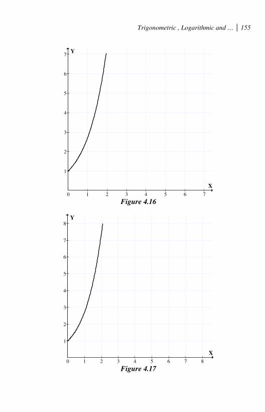
Trigonometric , Logarithmic and … 155
0 1 2 3 4 5 6 7
1
2
3
4
5
6
7
X
Y
Figure 4.16
0 1 2 3 4 5 6 7 8
1
2
3
4
5
6
7
8
X
Y
Figure 4.17

156 MOD Functions
So for the MOD exponential function e
x; x = 2 we have the
smallest MOD plane to be Rn(8) and the all MOD planes in which
x = 2 and 0 ≤ x < 3 accommodated is Rn(20).
So nex; 0 ≤ x ≤ 3 can fit in the MOD plane Rn(21). The MOD
exponential graph of the function nex; 0 ≤ x ≤ 3 is as follows.
0 2 4 6 8 10 12 14 16 18 20
2
4
6
8
10
12
14
16
18
20
X
Y
Figure 4.18
So the smallest MOD plane which can accommodate the
MOD exponential function nex; 0 ≤ x ≤ 3 in Rn(21).
All MOD planes Rn(m), 3 ≤ m ≤ 54 can accommodate only
MOD exponential function nex; 0 ≤ x ≤ 3 where x = 4 that is for
MOD exponential functions nex; 0 ≤ x ≤ 4 the smallest MOD
plane which can accommodate is Rn(55).
All MOD planes Rn(m) 3 ≤ m ≤ 148 can accommodate only
MOD exponential functions nex; 0 ≤ x ≤ 4.

Trigonometric , Logarithmic and … 157
It is pertinent to keep on record that for a very small or
considerably small x of the MOD exponential function nex one
needs a very large MOD plane for it to be defined.
For instance for x = 9, that is 0 ≤ x ≤ 9 of the MOD
exponential function nex; one needs the smallest MOD plane to
be Rn(8104).
For 0 ≤ x ≤ 8 of the MOD exponential function nex one needs
the smallest MOD plane to be Rn(2981).
One can see for a very small variation of 1 in the value of x
nearly there is an increase of 5000 in m in the MOD plane Rn(m).
For x = 10 the smallest MOD plane in which nex is defined is
Rn(22027).
So for the change of 1 from 9 to 10 of x in nex the change in
m is 22027 – 8104 = 13,923.
Thus the way nex grows or to be more precise e
x grows is
seen from the study of finding the smallest MOD planes.
Having seen the definition of MOD exponential function
now we proceed onto define the notion of MOD hyperbolic
function.
The MOD hyperbolic trigonometric function in the MOD
plane Rn(m); 3 ≤ m < ∞ is in
sinhx = x (m 1)xe (m 1)e
2
−+ −
ncoshx = x (m 1)xe e
2
−+
ntanhx = x (m 1)x
x (m 1)x
e (m 1)e
e e
−
−
+ −
+

158 MOD Functions
ncothx = x (m 1)x
x (m 1)x
e e
e (m 1)e
−
−
+
+ −
nsechx = x (m 1)x
2
e e −+
and
ncosechx = x (m 1)x
2
e (m 1)e −+ −.
It is important at this juncture to keep on record it is not an
easy task to trance these MOD hyperbolic trigonometric
functions.
In fact research in this direction left open.
Next here we just introduce the notion of MOD logarithmic
functions.
Since for every x ∈ R\{0} log x is defined. Here we define
mainly for the base 10 the MOD logarithmic function.
In the first place if Rn(m) is the MOD plane and R a real
plane we have a MOD transformation from R to Rn(m).
Now the graph of usual log10 base function has the
following graph in reals is given in Figure 4.19.
However in the MOD plane Rn(60) the MOD log10x denoted
by nlogx is given in Figure 4.20.

Trigonometric , Logarithmic and … 159
10 20 30 40 50 60 70 80 90 1000
10
20
30
40
50
60
70
80
90
100
X
Y
Figure 4.19
0 10 20 30 40 50 600
10
20
30
40
50
60
X
Y
Figure 4.20

160 MOD Functions
So the MOD logarithmic graph is not an infinite curve
depending on m of the Rn(m) it will be long or short however
certainly there is no change in the curve so the first quadrant of
real plane can be sliced depending on m and the same curve will
serve the purpose as t ∈ [0, m) for any MOD real plane Rn(m).
Authors leave open the problems related with MOD
logarithmic functions. Here only study or definition is made
with respect to base 10.
However it is not difficult to obtain new logarithmic
functions for any suitable base.
This work is left as an exercise to the reader.

Chapter Five
NEUTROSOPHIC MOD FUNCTIONS AND OTHER MOD FUNCTIONS
In this chapter we define neutrosophic MOD functions (or
small neutrosophic functions) using neutrosophic MOD planes,
neutrosophic MOD complex modulo integer functions, MOD dual
number functions, MOD special dual like number functions and
MOD quasi dual like number functions using the MOD
neutrosophic complex modulo integer plane I
nC (m) , MOD dual
number plane Rn(m)(g) with g2 = 0, MOD special dual like
number plane Rn(m)h, h2 = h and MOD special quasi dual
number plane Rn(m)k; k2 = (m – 1) k respectively.
These situations will be described by examples as the
definitions can be easily done analogous to functions in chapter
II and III.
Example 5.1: Let I
nR (9) = {a + bI | a, b ∈ [0, 9); I2 = I} be the
MOD neutrosophic plane.
Let
I
nR (9)[x] = i
i
i 0
a x∞
=
∑ ai ∈ I
nR (9) }

160 MOD Functions
be the MOD neutrosophic polynomial. Every polynomial p(x) ∈ I
nR (9)[x] is a MOD neutrosophic function or small neutrosophic
function.
p(x) = 3.5Ix3 + (4 + 2.5I)x + (7 + 3I) is a MOD neutrosophic
polynomial function.
p(x) can be differentiated as well as integrated.
Some polynomial functions may not be integrable or
derivable.
dp(x)
dx = 3 (3.5)Ix
2 + (4 + 2.5I)
= 1.5Ix2 + (4 + 2.5I).
2
2
d p(x)
dx= 3Ix + 0
3
3
d p(x)
dx = 3I.
Thus as in case of usual polynomials over reals this MOD
neutrosophic polynomial has all the derivatives.
Example 5.2: Let I
nR (6)[x] be the set of all MOD neutrosophic
polynomials. Every p(x) ∈ I
nR (6)[x] is a MOD polynomial
neutrosophic functions.
Let
p(x) = 3x4 + (4 + 2I)x
3 + (2.3 + 0.75I) ∈ I
nR (6) .
p′(x) = dp(x)
dx = 0 (mod 6).
So natural form of differentiation is true for this function.
Another importance about these functions is the roots of the
MOD neutrosophic polynomials.

Neutrosophic MOD Functions … 161
Consider
p(x) = (x + 2 + 4I) × (x + 3.5I) × (x + 0.8) ∈ I
nR (6)[x] .
Clearly if x = 4 + 2I then p(4 + 2I) = 0.
If x = 2.5I then also consider p(2.5I) = 0.
If x = 5.2 then p(x) = p(5.2) = 0.
Now consider
(x + 2 + 4I) (x + 3.5I) (x + 0.8)
= [x2 + (2 + 4I)x + 3.5Ix + (2 + 4I) (3.5I)] (x + 0.8)
= (x2 + (2 + 1.5I)x + 3I) (x + 0.8)
= x3 + (2 + 1.5I)x
2 + 3Ix + 0.8x
2 + (1.6 + 1.2I)x + 2.4I
= x3 + (2.8 + 1.5I)x
2 + (1.6 + 4.2I)x + 2.4I = q(x).
q(4 + 2I)
= (4 + 2I)3 + (2.8 + 1.5I) (4 + 2I)
2 + (1.6 + 4.2I) + 2.4I
= (16 + 4I + 16I) (4 + 2I) + (2.8 + 1.5I) (2I + 4) +
(6.4 + 4.8I + 3.2I + 2.4I) + 2.4I
= 4 + 2I + (5.2 + 3I + 5.6I) + 0.4 + 0.8I
= 3.6 + 5.4I
≠ 0.
In the first place
p(x) ≠ q(x).
When the polynomial is expanded 4 + 2I fails to be a root of
q(x).
Now
q(2.5I) = (2.5I)3 + (2.8 + 1.5I) 2.5I + (1.6 + 4.2I) (2.5I) + 2.4I
= 0.625I + I + 3.75I + 4.00I + 10.50I + 2.4I ≠ 0.

162 MOD Functions
So 2.5I is not a root of q(x).
Finally consider
q(5.2) = (5.2)3 + (2.8 + 1.5I) (5.2)
2 + (1.6 + 4.2I) 5.2 + 2.4I
= 2.608 + 2.512 + 4.56I + 2.32 + 3.84I + 2.4I ≠ 0.
Hence 5.2 is also not a root of q(x).
Thus we see all the 3 roots of p(x) are not roots of q(x)
though q(x) is got only by multiplying the three linear
polynomials.
Thus it remains as a open conjecture finding the roots of the
MOD neutrosophic functions.
The problem is doubled as the MOD neutrosophic
polynomials is only a pseudo ring.
Example 5.3: Let I
nR (5)[x] be the MOD neutrosophic
polynomial pseudo ring.
p(x) = (x + 2I + 3) (x + 4I) ∈ I
nR (5)[x] .
p(x) = (x + 2I + 3) (x + 4I)
so the roots of p(x) are 3I + 2 and I.
p(3I + 2) = 0 and p(I) = 0.
Let
q(x) = (x + 2I + 3) (x + 4I)
= x2 + 2Ix + 3x + 4Ix + 8I + 12I
= x2 + (I + 3)x.
q(I) = I2 + I + 3I = 0.

Neutrosophic MOD Functions … 163
So I is a root of q(x).
q(3I + 2) = (3I + 2)2 + (I + 3) (3I + 2)
= 9I + 6I + 6I + 4 + 3I + 9I + 2I + 6
= 0.
So 3I + 2 is also a root and p(x) = q(x).
The main reason for this is p(x) ∈ ⟨Z5 ∪ I ⟩[x] so is
neutrosophic ring.
Consider p(x) = (x + 0.3 + 0.7I) (x + 0.8) × (x + 0.3I + 2).
Clearly x = 4.7 + 4.3I, x = 5.2 and x = 3 + 4.7I are roots of
p(x).
For p(4.7 + 4.3I) = 0,
p(5.2) = 0 and p(3 + 4.7I) = 0
But
(x + 0.3 + 0.7I) (x + 0.8) (x + 2 + 0.3I)
= (x2 + 0.3x + 0.7Ix +0.8x + 0.24 + 0.56I) (x + 2 + 0.3I)
= x3 + 0.3x
2 + 0.7Ix
2 + 0.8x
2 + 0.24x + 0.56I + 2x
2 + 0.6x
+ 1.4Ix + 1.6x + 0.48 + 1.12I + 0.3Ix2 + 0.09Ix + 0.21Ix
+ 0.24Ix + 0.072I + 0.168I
= x3 + (0.3 + 0.7I + 0.8 + 2 + 0.3I)x
2 + (0.24 + 0.6 + 1.4I
+ 1.6 + 0.09I + 0.21I + 0.24I)x + 0.56I + 0.48 + 1.12I +
0.168I + 0.072I
= x3 + (3.1 + I)x
2 + (1.9 + 1.94I)x + (0.48 + 1.92I) = q(x).
q(4.7 + 4.3I) = (4.7 + 4.3I)3 + (3.1 + I) (4.7 + 4.3I)
2 +
(1.9 + 1.94I) (4.7 + 4.3I) + (0.48 + 1.92I)

164 MOD Functions
= (2.09 + 3.49I +0.42I) (4.7 + 4.3I) + (2.09 + 3.49I +
0.42I) (I + 3.1) + (3.93 + 4.118I + 3.17I + 3.342I) +
0.48 + 1.92I
= (4.823 + 3.987I + 3.377I + 1.813I) + (2.09I + 3.91I +
1.479 + 2.121I) + 4.41 + 2.550I
= 0.742 + 4.848I ≠ 0.
So 4.7 + 4.3I is not a root of q(x).
q(5.2) = (5.2)3 + (3.1 + I) (5.2)
2 + (1.9 + 1.94I) (5.2) +
(0.48 + 1.92I)
= 0.608 + 2.04I + 1.324 + 4.88 + 0.88I + 0.48 + 1.92I
= 2.292 + 4.84I ≠ 0.
So x = 5.2 is not a root of q(x).
q(3 + 4.7I) = (3 + 4.7I)3 + (3.1 + I) (3 + 4.7I)
2 +
(1.9 + 1.94I) (3 + 4.7I) + (0.48 + 1.92I)
= 2 + (4.7I)3 + 2 × 4.7I + 4 × (4.7I)
2 + 3.1 × 4 + 4I + 3.1 ×
(4.7)2I + (4.7)
2I + 4.7I + 3.1 × 4.7I + 0.7 + 0.82I + 1.9 ×
4.7I + 1.94 × 4.7I + 0.48 + 1.92I
= (2 + 2.4 + 0.7 + 0.48) + (4.7I + 3.823I + 4.4I + 3.36I +
4I + 3.479I + 2.09I + 4.57I + 0.82I + 3.93I + 4.118I +
1.92I)
= 0.58 + 1.21I ≠ 0.
Thus 3 + 4.7I is also not a root of q(x).
None of the roots of p(x) is a root of q(x) as the distributive
law is not true in I
nR (5)[x] .

Neutrosophic MOD Functions … 165
Thus solving for roots happens to be a very difficult task in
this case.
So in case of MOD neutrosophic functions the problem of
solving equations is as difficult as that of solving MOD real
functions.
Next we proceed on to work with functions on MOD
complex neutrosophic modulo integers; I
nC (m)[x] .
I
nC (m) = {a0 + a1I + a2iF + a3iFI | a0, a1, a2, a3 ∈ [0, m)}
( 2
Fi = m–1, I2 = I).
I
nC (m)[x] = i
i
i 0
x∞
=
α
∑ αi ∈ I
nC (m) }
is the MOD neutrosophic complex modulo integer pseudo
polynomial ring [24].
Example 5.4: Let x2 + 3iF + 4.3I ∈ I
nC (10)[x] . Solve for x.
x2 = 7iF + 5.7I, x = F7i 5.7I+ .
Finding roots of these values happen to be a open
conjecture.
However as I2 = I one can say I = I.
Apart from this finding root of F7i 5.7I+ remains a
challenging problem.
Let p(x) = (3 + 0.7iF + 5iFI)x3 + (7.2I + 4iF + 2)x +
4 + 5IiF + 8.9iF + 4I be a function in I
nC (10)[x] .
dp(x)
dx = (3 (3 + 0.7iF + 5iFI)x
2 + (7.2 + 4iF + 2)

166 MOD Functions
2
2
d p(x)
dx = 2 (9 + 2.1iF + 5iFI)x + 0
= (8 + 4.2iF)x.
3
3
d p(x)
dx = 8 + 4.2iF.
Now for the integral
∫p(x) dx = 4
F F(3 0.7i 5i I)x
4
+ + +
2
F(7.2I 4i 2)x
2
+ ++
(4 + 5IiF + 8.9iF + 4I) x + C
However the first two terms are not defined as 4 and 2 are
zero divisors in I
nC (10). So one cannot say given a function in I
nC (10)[x] its integral will exist.
It may exist or at times may not be defined.
Example 5.5: Let
p(x) = x7 + 0.3x
2 + 1.4Ix + (2.5 + 0.7iF) ∈ I
nC (7)[x]
be a MOD polynomial function in I
nC (7)[x] .
Finding roots of p(x) is a challenging problem.
dp(x)
dx = 0.6x + 1.4I.
So a seventh degree MOD polynomial in I
nC (7)[x] has its first
derivative to be a polynomial in x.
Thus the usual laws of derivatives are not in general true for
the MOD polynomials.

Neutrosophic MOD Functions … 167
Let p(x) = 3.5Ix2 + (1.7I + 2.3iF) ∈ I
nC (7)[x] .
The derivative dp(x)
dx= 0.
So its derivative is zero however p(x) is not a constant MOD
polynomial.
Now ∫ p(x) dx = 33.5Ix
3 + (1.7I + 2.3iF)x + C
= 3.5Ix3 + (1.7I + 2.3iF)x + C.
Thus the integral of this MOD polynomial function is well
defined and the integral exist.
Let a(x) = (3.5 + 4.2iF + 3I + 2.1iFI)x6 ∈ I
nC (7)[x] .
Clearly ∫a(x) dx = 7
F F(3.5 4.2i 3I 2.1Ii )x
7
+ + + + C.
Thus the integral is not defined as 1
7 is undefined in
I
nC (7)[x] .
However da(x)
dx = 6(3.5 + 4.2iF + 3I + 2.1iFI)x
5
= (4.2iF + 4I + 5.6IiF)x5 exist and is well defined.
2
2
d a(x)
dx = 5(4.2iF + 4I + 5.6iFI)x
4
= 6I x4.

168 MOD Functions
3
3
d a(x)
dx = 6I × 4x
3
= 3x3.
4
4
d a(x)
dx = 2x
2
5
5
d a(x)
dx = 4x
and 6
5
d a(x)
dx = 4 a constant.
However we started with a coefficient from I
nC (7) and it
has all the 4 terms real complex modulo factor iF, neutrosophic
factor I and the combination of both.
However the 6th derivative gave only a constant which is a
real integer 4.
Example 5.6: Let s(x) = 3iFx4 + (4 + 0.5I + 2iF)x
3 +
(4.2 + 3iFI)x + (2.3 + 4.8iF + 0.3iFI + 5.12I) ∈ I
nC (6)[x] be a
MOD polynomial function with neutrosophic modulo complex
number coefficients.
ds(x)
dx = 4 × 3iFx
3 + 3 (4 + 0.5I + 2iF)x
2 + (4.2 + 3iFI)
= (1.5I)x2 + (4.2 + 3iF) I.
2
2
d s(x)
dx = 3Ix + 0

Neutrosophic MOD Functions … 169
3
3
d s(x)
dx = 3I and
4
4
d s(x)
dx = 0.
However this MOD function is a forth degree polynomial so
the forth derivative must be a constant under natural or usual
condition.
Now
∫s(x) dx = 5 4 2
F F F3i x (4 0.5I 2i )x (4.2 3i )x
5 4 2
+ + ++ +
+ (2.3 + 4.8iF + 0.3iFI + 5.12I)x + C.
But ∫s(x) dx is not defined as 1
4 and
1
2 are not defined in
I
nC (6)[x] .
Thus the integral does not exist.
So MOD polynomial neutrosophic complex modulo integer
functions behave in a very different way from the usual
polynomial functions.
It is left as an open conjecture to solve equations in the MOD
complex neutrosophic functions.
The problem occurs mainly because the collection I
nC (m)[x] is only a pseudo polynomial ring.
So (x + a0 + a1I + a2iF + a3IiF) × (x + b0 + b1I + b2iF + b3IiF) ×
(x + c0 + c1I + c2iF + c3IiF) ≠ x3 + (α1 + α2 + α3)x
2 + … +
α1 α2 α3;
where
α1 = a0 + a1I + a2iF + a3IiF
α2 = b0 + b1I + b2iF + b3IiF
and α3 = c0 + c1I + c2iF + c3IiF.
Let p(x) = (x + 0.3 + 4iF + 5.1iFI) × (x + 7 + 0.8I + 4.2iF) ∈ I
nC (8)[x] .

170 MOD Functions
p(x) = x
2 + [(0.3 + 4iF + 5.1iFI) + (7 + 0.8I + 4.2iF)] +
(0.3 + 4iF + 5.1iFI) (7 + 0.8I + 4.2iF)
= x2 + (7.3 + 0.2iF + 0.8I + 5.1iFI)x + (2.1 + 4iF +
3.7iFI + 0.24I + 0.32IiF + 4.08iFI + 5.94I + 4.6iF
+ 5.6)
= x2 + (7.3 + 0.2iF + 0.8I + 5.1iFI)x + (7.7 + 0.6iF +
6.18I + 0.10iFI)
= q(x).
The roots of p(x) are
x = 7.7 + 4iF + 2.9iFI
and
x = 1 + 7.2I + 3.8iF.
p(7.7 + 4iF + 2.9iFI) = 0
and
q(7.7 + 4iF + 2.9iFI)
= (7.7 + 4iF + 2.9iFI)2 + (7.3 + 0.2iF + 0.8I + 5.1IiF) ×
(7.7 + 4iF + 2.9iFI) + (7.7 + 0.6iF + 6.18I + 0.1iFI)
= (5.9 + 2.87I + 4.66IiF) + (0.21 + 1.54iF + 6.16I +
7.27IiF + 5.2iF + 5.6 + 3.2IiF + 4.4I + 5.17iFI +
2.32I + 2.32iFI + 7.53I) + (7.7 + 0.6iF + 6.18I +
0.1iFI)
= (3.41 + 5.46I + 7.34iF + 6.72IiF)
≠ 0.
So p(x) ≠ q(x) and the root of p(x) is not the same as that of q(x)
and vice versa.
Next we proceed onto define the notion of MOD real dual
number functions.

Neutrosophic MOD Functions … 171
Rn(m)(g) = {a + bg | g
2 = 0, a, b ∈ [0, m)} is defined as the
MOD real dual number plane.
We will just for the sake of completeness describe the
plane.
Let Rn(5)g be the MOD real dual number plane.
The point 3 + 2.5g = (3, 2.5).
0.5 1 1.5 2 2.5 3 3.5 4 4.5 5 5.50
0.5
1
1.5
2
2.5
3
3.5
4
4.5
5
5.5
X
g
(3,2.5)
Figure 5.1
Clearly Rn(m)(g) is only a MOD real dual number pseudo
ring.
Consider
Rn(m)g[x] = i
i
i 0
a x∞
=
∑ ai ∈ Rn(m)g, g
2 = 0}.

172 MOD Functions
Rn(m)g[x] is defined as the collection of MOD dual number
coefficient polynomials Rn(m)g[x] is only a pseudo ring.
Any p(x) ∈ Rn(m)g[x] is a MOD polynomial function in the
variable x.
One can differentiate and integrate these MOD functions
only whenever they exist and are defined.
We will illustrate these situations by some examples.
Example 5.7: Let
Rn(10)g[x] = i
i
i 0
a x∞
=
∑ ai ∈ Rn(10)g = {a + bg | a, b ∈ [0, 10),
g2 = 0}} be the MOD dual number polynomial pseudo ring.
Let f(x) = (2.3 + 0.7g)x3 + (3.2 + 5.1g)x
2 + (2.17 + 3.89g) ∈
Cn(10)g[x].
df (x)
dx = (3 (2.3 + 0.7g)x
2 + 2(3.2 + 5.1g)x
= (6.9 + 2.1g)x2 + (6.4 + 0.2g)x.
2
2
d f (x)
dx = 2 (6.9 + 2.1g)x + (6.4 + 0.2g)
= (3.8 + 4.2g)x + (6.4 + 0.2g).
Thus the derivative of f(x) exists.
∫f(x) dx = 4 3(2.3 0.7g)x (3.2 5.1g)x
4 3
+ ++ + (2.17 + 3.89g)x + C
Clearly ∫f(x) dx does not exist as 1
4 is not defined in [0, 10).

Neutrosophic MOD Functions … 173
Thus it is important to keep on record that the derivative
may exist but the integral may not exist.
Similarly there may be MOD polynomials in which integrals
may exist but the derivatives may not exist.
Study of these MOD functions is an interesting task.
Now we will proceed onto study the roots of these MOD
functions.
Example 5.8: Let
Rn(7) g[x] = i
i
i 0
a x∞
=
∑ ai ∈ Rn(7)g = {a + bg | a, b ∈ [0, 7), g
2 =
0}} be the MOD dual number pseudo polynomial function ring.
Let p(x) = x + 3.25 + 6.08g ∈ Rn(7)g[x] only root of p(x) is
x = 3.75 + 0.92g.
Now let p(x) = (x + 6.5) (x + 2 + 4.5g) ∈ Rn(7)g[x].
The roots of p(x) are x = 0.5 and x = 5 + 2.5g
p(0.5) = 0 and p(5 + 2.5g) = 0.
Consider
q(x) = (x + 6.5) (x + 2 + 4.5g)
= x2 + 6.5x + 2x + 4.5gx + 6 + 1.25g
= x2 + (1.5 + 4.5g)x + 0.25g.
q(0.5) = (0.5)2 + (1.5 + 4.5g) 0.5 + 0.25g
= 0.25 + 0.75 + 2.25g + 0.25g
= 1 + 2.5g ≠ 0.
So 0.5 is not a root of q(x).
q(5 + 2.5g) = (5 + 2.5g)2 + (1.5 = 4.5g) (5 + 2.5g) + 0.25g
= 4 + 4g + 0.5 + 1.5g + 3.75g + 0.25g

174 MOD Functions
= 4.5 + 2.5g ≠ 0.
Thus 5 + 2.5g is not a root of q(x).
Hence the problem of finding roots for these MOD
polynomial functions happens to be a challenging work.
Next we proceed onto define the notion of MOD special dual
like number functions built using the MOD special dual like
number plane Rn(m)g; g2 = g.
Figure 5.2

Neutrosophic MOD Functions … 175
Define
Rn(m)g[x] = i
i
i 0
a x∞
=
∑ ai ∈ Rn(m)g; g
2 = g
where Rn(m)g = {a + bg | a, b ∈ [0, m)}} to be the collection of
all MOD special dual like number functions.
Clearly Rn(m)g[x] is a pseudo ring.
Here through examples we show how these MOD special
dual like functions behave.
Example 5.9: Let
Rn(12)g[x] = i
i
i 0
a x∞
=
∑ ai ∈ Rn(12)g; = {a + bg | g
2 = g, a, b ∈
[0, 12)}} be the collection of all MOD functions.
Solving equations are difficult as
p(x) = (x + α1) (x + α2) (x + α3) (x + α4)
≠ x4 + (α1 + α2 + α3 + α4)x
3 + (α1α2 +α1α3 + α1α4 + α3α2 +
α2α4 + α4α3 )x2 – (α1α2α3 +α1α2α4 + α1α3α4 + α2α3α4)x
+ α1α2α3α4 = q(x).
So roots of p(x) are not roots of q(x). It is difficult to find
roots; for the situation in case of MOD polynomials happens to
be a challenging one.
Next integrating or differentiating these functions is also a
difficult task.
For let
f(x) = (3.4 + 4.5g)x4 + (4 + 8g)x
3 + (2.5 + 3.5g)x
2
+ (7.1 + 10.3g) ∈ Rn(12) g[x].

176 MOD Functions
f ′(x) = 4(3.4 + 4.5g)x3 + 3(4 + 8g)x
2 + 2 (2.5 + 3.5g)x
= (1.6 + 6g)x3 + (5 + 7g)x
f ′ (x) = 3 (1.6 + 6g)x2 + 5 + 7g
= (4.8 + 6g)x2 + 5 + 7g
f ″′ (x) = 2(4.8 + 6g)x
= 9.6x.
f4(x) = 9.6.
Thus the fifth derivative is zero.
Now
∫f(x) dx = 5 4 3(3.4 4.5g)x (4 8g)x (2.5 3.5g)x
5 4 3
+ + ++ +
+ (7.1 + 10.3)gx + C.
Clearly 1
4 or
1
3 is not defined in [0, 12) so the integral does
not exist.
Consider s(x) = 5.2x12
+ (6g + 4)x6 + (4.5 + 2.3g)x
3 + 5g
s′(x) = 12 × 5.2x11
+ 6(6g + 4)x5 + 3(4.5 + 2.3g)x
2 + 0
= 2.4x11
+ (1.5 + 6.9g)x2 .
s″(x) = 2.4 × 11x10
+ 2(1.5 + 6.9g)x
= 2.4x10
+ (3 + 1.8g)x.
We can find the 3rd
derivative
3
3
d s(x)
dx = 10 × 2.4x
9 + (3 + 1.8g)

Neutrosophic MOD Functions … 177
= 3 + 1.8g.
The forth derivative is zero.
However this MOD function is a polynomial of degree 12
and the forth derivative zero is not in keeping with the usual
form of differentiation.
Next we find the integral of s(x).
∫s(x) dx = 13 7 45.12x (6g 4)x (4.5 2.3g)x
5gx C13 7 4
+ ++ + + +
Clearly this integral is also not defined as 1
4 is not defined in
the MOD interval [0, 12).
Example 5.10: Let Rn(10)g[x] = i
i
i 0
a x∞
=
∑ ai ∈ Rn(10)g =
{a + bg | a, b ∈ [0, 10), g2 = g}} be the collection of MOD dual
like number polynomial functions.
Let p(x) = (6.2 + 4.3g)x6 + 0.2x
5 + (5 + 2g)x
2 + (7 + 3g) ∈
Rn(10)g[x].
p′(x) = 6(6.2 + 4.3g)x5 + x
4 + 2(5 + 2g)x
= (7.2 + 5.8g)x5 + x
4 + 4gx.
If the integration and differentiation are the inverse process of
each other.
We find ∫p′(x) dx
6 5 2(7.2 5.8g)x x 4gx
6 5 2
++ + .

178 MOD Functions
Clearly ∫p′(x) dx is not defined.
However we find
∫p(x) dx = 7(6.2 4.3g)x
7
+ +
6 30.2x (5 2g)x
6 3
++ +
(7 + 3g)x + C.
Clearly ∫p(x) dx is also not defined.
Thus d( p(x)dx) dp(x).dx.
dx dx
∫≠ ∫
in general for any MOD polynomial function in Rn(10)g[x].
Example 5.11: Let Rn(7)g[x] = i
i
i 0
a x∞
=
∑ ai ∈ Rn(7)g = {a + bg |
a, b ∈ [0,7), g2 = g}} be the MOD special dual like number
functions.
Let p(x) = (6.3 + 2g)x5 + (3 + 6.5g)x
3 + (4 + 2g) ∈
Rn(7)g[x].
p′(x) = 5(6.3 + 2g)x4 + 3(3 + 6.5g)x
2
= (3.5 + 3g)x4 + (2 + 5.5g)x
2 .
∫p′(x) dx = 5 3(3.5 3g)x (2 5.5g)x
C5 3
+ ++ +
= (3.5 + 2g)x5 + (3 + 6.5g)x
3 + C
≠ p(x).

Neutrosophic MOD Functions … 179
∫p (x) dx = 6 4(6.3 2g)x (3 6.5g)x
6 4
+ ++ + (4 + 2g)x + C
= (2.8 + 5g)x6 + (6 + 6g)x
4 + (4 + 2g)x + C.
d( p(x)dx)
dx
∫ = 6 (2.8 + 5g)x
5 + 4(6 + 6g)x
3 + (4 + 2g)
= (2.8 + 2g)x5 + (3 + 3g)x
3 + 4 + 2g
≠ p(x).
Hence
d( p(x)dx)
dx
∫≠ p(x)
∫p′(x) dx ≠ p(x).
Thus in no way one can relate the MOD functions
derivatives and integrals.
Next the concept of special quasi dual number functions is
described by some examples.
Let Rn(m)g[x] = i
i
i 0
a x∞
=
∑ ai ∈ Rn(m)g = {a + bg | a, b ∈
[0,m) and g2 = (m–1)g}} be the collection of all MOD special
quasi dual number polynomial functions.
Clearly ∫p′(x) dx ≠ p(x).
d
p(x)dxdx ∫ ≠ p(x) in general.
Further the roots of these MOD polynomial with special
quasi dual number coefficients behave in a chaotic way.

180 MOD Functions
These situations are described by an example or two.
Example 5.12: Let
Rn(9)g[x] = i
i
i 0
a x∞
=
∑ ai ∈ Rn(9)g = {a + bg | a, b ∈ [0,9) and
g2 = 8g}} be the collection of all MOD polynomials functions
with coefficients from the special quasi dual number Rn(9)g.
Let
p(x) = x + (3.7 + 2.5g) ∈ Rn(9)g[x].
The root of p(x) is
x = 5.3 + 6.5g.
Consider
q(x) = x2 + 7.2 + 4.3g ∈ Rn(9)g[x]
find the roots of q(x) is a difficult task.
Let
p(x) = (x + 3 + 6.5g) (x + 2.1 + 3g) ∈ Rn(9)g[x].
The roots of p(x) are x = 6 + 2.5g and x = 6.9 + 6g
Consider
(x + 3 + 6.5g) (x + 2.1 + 3g)
= x2 + 3x + 6.5gx + 2.1x + 6.3 + 4.65 + 3gx + 0
+ 1.5x × 8g
= x2 + (5.1 + 0.5g)x + 4.95
= q(x).
is x = 6 + 2.5g and x = 6.9 + 6g roots of q(x).
q(6 + 2.5g) = (6 + 2.5g)2 + (5.1 + 0.5g) (6 + 2.5g) + 4.95
= 6.25 × 4g + 7.5g + 3.6 + 3g + 3.75g + g + 4.95

Neutrosophic MOD Functions … 181
= 4.25 + 8.55 ≠ 0.
So 6 + 2.5g is not a root.
Let us consider
q(6.9 + 6g)
= (6.9 + 6g)2 + (5.2 + 0.5g) × (6.9 + 6g) + 4.95
= 2.61 + 1.8g + 8.19 + 3.6g + 6g + 7.5g + 4.95
= 7.75 + 0.9g ≠ 0.
So 6.9 + 6g is also not a root of q(x).
Let us consider the MOD polynomial function.
p(x) = (3.6 + 4.2g)x6 + (2.1 + 0.6g)x
4 + (4.5 + 2.5g)x
2
+ (5 + 7g) ∈ Rn(9)[x].
p′(x) = 6(3.6 + 4.2g)x5 + 4(2.1 + 0.6g)x
3 + 2(4.5 + 2.5g)x
= (3.6 + 7.2g)x5 + (8.4+ 2.4g)x
3 + 5gx.
∫p′(x) dx = 6 4 2(3.6 7.2g)x (8.4 2.4g)x 5gx
6 4 2
+ ++ + + C
≠ p(x).
∫p′(x) dx is not defined as 1
6 is not defined in [0, 9).
∫p(x) dx = 7 5 3(3.6 4.2g)x (2.1 0.6g)x (4.5 2.5g)x
7 5 3
+ + ++ +
+ (5 + 7g)x + C.

182 MOD Functions
This is not defined as 1
3 is not defined in [0, 9).
Thus the natural laws of derivative and integral are not in
general true in case of MOD function.
Now we proceed onto define some new types of MOD
functions.
Let f be a MOD function defined on the MOD real plane or
MOD neutrosophic plane or MOD complex modulo integer plane
or MOD neutrosophic complex modulo integer plane or MOD
dual number plane or MOD special dual like number plane or
MOD special quasi dual number plane.
We say f is a special dual MOD function if f o f = 0.
We call f a special dual like MOD function if f o f = f.
We call f to be a special quasi dual function if
f o f = (m – 1)f
where f is defined over the MOD plane relative to the interval
[0, m).
It is left as an exercise for the reader to construct examples
of these new type of MOD functions.

Chapter Six
SUGGESTED PROBLEMS In this chapter we suggest a few problems for the reader. Some
of them are difficult and some of them are simple and some are
open problems.
1. Obtain some interesting properties enjoyed by decimal
polynomial rings in the MOD plane.
2. Why the MOD differentiation is different from that of
usual differentiation in case of functions in the MOD
plane?
3. Prove by an example a function which is continuous in
R is not continuous in the MOD plane Rn(m).
4. What are the special and interesting features enjoyed by
functions in the MOD plane?
5. Study the function y = 5x + 3 ∈ R[x] in the MOD plane
Rn(7) and Rn(4).
(i) Are they continuous in these planes?
(ii) What are the zeros in these MOD functions?
(iii) When is the function differentiable?

184 MOD Functions
(iv) Does there exist a MOD function f(x) whose
derivative f ′(x) exists?
(v) Can this function have infinite number of zero
divisors in any MOD plane?
(vi) Does there exists a MOD plane in which the function
y = 5x + 3 has only 5 zero divisors?
6. Let y = 7x2 + 3x + 1 ∈ R[x] be the function in the real
plane.
Study questions (i) to (vi) of problem 5 for y in the MOD
planes Rn(7), Rn(3), Rn(5) and Rn(10).
7. Let y = 3x3 – 7 ∈ R[x] be the function in the real plane.
Study questions (i) to (vi) of problem 5 in the MOD
planes Rn(7), Rn(2) and Rn(6).
8. Let y = 3x3 + 2x
2 – 5x + 8 ∈ R[x] be the function.
Study questions (i) to (vi) of problem 5 in the MOD
planes Rn(6), Rn(8), Rn(5), Rn(10) and Rn(4).
9. Let y = x2 + 4 ∈ R[x] be the function.
Study questions (i) to (vi) of problem 5 in the MOD
planes Rn(3), Rn(7) and Rn(4).
10. Let y = 9x5 – 3x
2 + 7 ∈ R[x] be the real function.
Study questions (i) to (vi) of problem 5 in the MOD
planes Rn(7), Rn(3), Rn(2) and Rn(10).
11. What is the difference in any function in the MOD
planes Rn(p) and Rn(m); p a prime and m is a non
prime?
12. Study question (11) for the function y = 7x3 – 5x + 1 in
Rn(11) and Rn(12).

Suggested Problems 185
13. Can all functions in the MOD plane Rn(m)[x] be
integrable?
14. How can we adopt integration and differentiation in
case of the functions in MOD plane Rn(m)[x]?
15. List out the difficulties in adopting integration to
functions in Rn(m)[x].
16. Prove derivatives of functions in Rn(m)[x] do not satisfy
the basic properties of derivatives.
17. Let f(x) = 5x7 + 5x
3 + 1.7x + 3 ∈ Rn(7)[x].
(i) Find f ′(x).
(ii) What is 7
7
d f (x)
dx ?
(iii) Find ∫ f(x) dx.
(iv) Is f(x) continuous in Rn(7)[x]?
(v) Can f(x) be continuous on Rn(6)[x]?
18. Does this MOD function f(x) = 6x3 + 7x
2 + 1 ∈ Rn(8)[x]
continuous in the MOD plane Rn(8).
19. Is f(x) ∈ Rn(8)[x] in problem 18 differentiable?
20. Is f(x) ∈ Rn(8)[x] in problem 18 integrable?
21. Give a function f(x) ∈ Rn(12)[x] which is both
differentiable and integrable.
22. Give a function f(x) ∈ Rn(10)[x] which is neither
integrable nor follow any properties of derivation?
23. Finding roots of a MOD polynomials in Rn(m)[x] is a
open problem.

186 MOD Functions
24. Prove MOD polynomials do not satisfy the fundamental
theorem of algebra;
“A nth degree polynomial has n and only n roots”
25. Give an example of a MOD polynomial of degree n
which has less than n roots.
26. Give an example of a MOD polynomial of degree n
which has more than n-roots.
27. Let p(x) = 8x8 + 5x
4 + 2 ∈ Rn(10)[x] be the MOD
polynomial.
Find all the roots of p(x).
28. Let p(x) = 5x3 + 3x + 1 ∈ Rn(7)[x] be the MOD
polynomial.
Find all the roots of p(x).
29. Is it possible to find all the roots of q(x) = x4 + 2 ∈
Rn(3)[x]?
(i) Can q(x) have more than 4 roots?
(ii) Does q(x) have less than four roots?
(iii) Find ∫ q(x) dx.
(iv) Find dq(x)
dx .
30. Let p(x) ∈ Rn(6)[x] where p(x) = x6 + 1.
Study questions (i) to (iv) of problem 29 for this p(x).
31. Find a polynomial in Rn(5)[x] of degree 3 which has
only three roots.
32. Find p(x) ∈ Rn(4)[x] be a polynomial of degree four
which has more than four roots.

Suggested Problems 187
33. Find a fifth degree polynomial in Rn(5)[x] which has
less than five roots.
34. Does there exist a MOD plane Rn(m) such that every
polynomial p(x) ∈ Rn(m)[x] follows the classical
properties of polynomials?
35. Let f(x) = 3x3 + 5x
2 + 1 ∈ Rn(10)[x].
Is f(x) a continuous function in the MOD plane Rn(10)?
36. Give an example of a function f(x) which is continuous
in R[x] but f(x) is not continuous in Rn(7)[x].
37. Let f(x) = x3 + 1 ∈ Rn(6)[x] be a MOD function.
(i) Is f(x) a continuous function?
(ii) Draw the graph of f(x) in the MOD plane Rn(6)?
(iii) Can f(x) = x3 + 1 be continuous in any other MOD
plane?
(iv) Can all the MOD planes in which the function
f(x) = x3 + 1 is continuous be characterized?
38. Let f(x) = 3x2 + 1 ∈ Rn(5)[x] be the MOD function.
Study questions (i) to (iv) of problem 37 for this f(x).
39. Obtain some special features enjoyed by MOD complex
plane Cn(m).
40. Prove every function in the complex plane C can be
transformed into a function in the MOD complex plane
Cn(m).
41. Let z ilimf (z)
→ where f(z) =
4z 1
z i
−
− ∈ C.

188 MOD Functions
Find the corresponding MOD function of f(z) in Cn(10),
Cn(7), Cn(16), Cn(11) and Cn(15).
42. Let f(z) = 2
2
z 8i
z 8z 8
−
− + ∈ C; limit z → 2 + 2i
(i) Find all the complex MOD planes Cn(m) in which
f(z) has a limit.
(ii) Find all these complex MOD planes Cn(m) in which
f(z) has no limit.
43. Does there exist a function in the complex plane which
has limit points for all values of z → z′ such that the
f(z) has limit for all z ∈ Cn(m)?
Justify your claim.
44. Let f(z) = 2
2
z z 2 i
z 2z 1
+ − +
− + ∈ C, let z → 1 + i be the
function in the complex plane.
Transform f(z) to the MOD planes (i) Cn(20), (ii) Cn(5),
(iii) Cn(7), (iv) Cn(4t) (v) Cn(16), (vi) Cn(29), (vii)
Cn(15) and (viii) Cn(21)
In which of these planes the limit exists?
45. Let f(z) = z2 + 1 be a MOD complex function in Cn(7).
(i) Is f(z) continuous in Cn(7)?
(ii) Is f(z) differential?
(iii) Find zeros of f(z).
46. Does there exist a function f(z) in Cn(5) which is
continuous in Cn(5)?
47. Obtain more properties related with MOD complex
functions.

Suggested Problems 189
48. When will a complex MOD function be continuous at all
points? Give one example of it.
49. f(x) = 3.75x3 + 0.4x + 3.28 ∈ Rn(4)[x] be a MOD
polynomial in Rn(4)[x].
(i) Find all roots of f(x).
(ii) Is f(x) a continuous function?
(iii) Does f(x) contain more than 3 roots?
(iv) Find all roots of f(x).
(v) Find a method by which these MOD equations can be
solved.
50. Solve p(x) = x3 + 1 ∈ Rn(5) [x].
51. Find roots of p(x) = x3 + 1 ∈ Rn(4)[x].
52. Find roots of p(x) in problems 50 and 52; which has
more zeros?
53. Let f(x) = x2 + 3 ∈ Rn(m), m = 4, 5, 6, 7, 8, 9, 10 and 11
be the MOD function.
(i) Find the plane Rn(m) in which f(x) has least number
of zeros; 4 ≤ m ≤ 11.
(ii) Find the plane Rn(m) in which f(x) has greatest
number of zeros; 4 ≤ m ≤ 11.
(iii) Is f(x) a continuous function?
(iv) Is f(x) an integrable function in Rn(m); 4 ≤ m ≤ 11?
(v) Is f(x) differential in Rn(m); 4 ≤ m ≤ 11?
(vi) Trace the function f(x) in all the MOD planes Rn(m);
4 ≤ m ≤ 11.
54. Let f(x) = x3 + 0.8 ∈ Rn(m); 2 ≤ m ≤ 15 be the MOD
function.
Study questions (i) to (vi) of problem 53 for this f(x).

190 MOD Functions
55. Let p(x) = 0.7x5.2
+ 0.9x0.2
+ 3 ∈ Rn(m); 4 ≤ m ≤ 10 be
the MOD function.
Study questions (i) to (vi) of problem 53 for this f(x).
56. Let f(z) = z2 + 0.3z + 1 ∈ Cn(m); 2 ≤ m ≤ 5 be the
complex MOD function.
(i) Is f(z) continuous in all planes?
(ii) Is f(z) differentiable?
(iii) Find lim f(z); z ∈ Cn(m), z → 1 + iF; 2 ≤ m ≤ 5.
57. Let f(z) = 3z2 + z + 1 ∈ Cn(m); 4 ≤ m ≤ 8 be the
complex MOD function.
Study questions (i) to (iii) of problem 56.
58. Obtain any special and interesting feature enjoyed by
complex MOD planes Cn(m), 2 ≤ m < ∞.
59. Derive the special identities related with MOD
trigonometric functions.
60. Obtain all the special features related with MOD
trigonometric functions.
61. What are the advantages of using MOD trigonometric
functions?
62. Draw the MOD graph of the MOD trigonometric function
yn = n tan x in the MOD plane Rn(10).
63. Draw the MOD graph of the MOD trigonometric function
yn = n tan 2x in the MOD plane Rn(10).
Compare the graphs in problems 62 and 63.
64. Draw the MOD trigonometric graph of the function
yn = n sin 3x in the MOD plane Rn(9).

Suggested Problems 191
65. Let yn = n cos 3x be the MOD trigonometric function.
Find the MOD graph of yn = n cos 3x in the MOD plane
Rn(19).
Compare yn = n cos 3x with yn = n sin 3x.
66. Prove or disprove nsin–1
x + ncos–1
x = π / 2 if x ∈ [0, 1].
67. Prove or disprove ntan–1
x + ncot–1
x = π / 2 if x ∈ [0, 1].
68. Prove or disprove nsec–1
x + ncos–1
x = π / 2 if x ∈
[0, 1].
69. Prove or disprove nsin–1
x + n sin–1
x =
n sin–1
(x 21 y− + y 21 x− ).
70. Find ntan–1
(n tan 3π /4).
71. Find n cos (n tan–1
¾).
72. Find ncos–1
(n cos 7π /6) ∈ Rn(m), m ≥ 9.
73. Find nsin (n cot–1
x).
74. Find nsin 2A.
75. Find n cos2A.
76. Is nsin2A =
1 n cos2A
2
−?
77. Obtain any interesting result about logarithmic MOD
functions.
78. Obtain the special features enjoyed by exponential MOD
functions.
79. Give examples of MOD neutrosophic real functions.
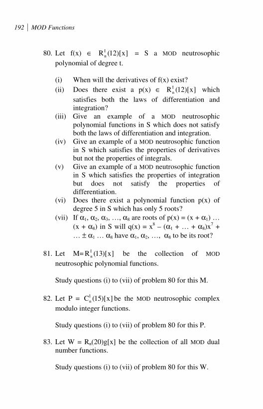
192 MOD Functions
80. Let f(x) ∈ I
nR (12)[x] = S a MOD neutrosophic
polynomial of degree t.
(i) When will the derivatives of f(x) exist?
(ii) Does there exist a p(x) ∈ I
nR (12)[x] which
satisfies both the laws of differentiation and
integration?
(iii) Give an example of a MOD neutrosophic
polynomial functions in S which does not satisfy
both the laws of differentiation and integration.
(iv) Give an example of a MOD neutrosophic function
in S which satisfies the properties of derivatives
but not the properties of integrals.
(v) Give an example of a MOD neutrosophic function
in S which satisfies the properties of integration
but does not satisfy the properties of
differentiation.
(vi) Does there exist a polynomial function p(x) of
degree 5 in S which has only 5 roots?
(vii) If α1, α2, α3, …, α8 are roots of p(x) = (x + α1) …
(x + α8) in S will q(x) = x8 – (α1 + … + α8)x
7 +
… ± α1 … α8 have α1, α2, …, α8 to be its root?
81. Let M= I
nR (13)[x] be the collection of MOD
neutrosophic polynomial functions.
Study questions (i) to (vii) of problem 80 for this M.
82. Let P = I
nC (15)[x] be the MOD neutrosophic complex
modulo integer functions.
Study questions (i) to (vii) of problem 80 for this P.
83. Let W = Rn(20)g[x] be the collection of all MOD dual
number functions.
Study questions (i) to (vii) of problem 80 for this W.

Suggested Problems 193
84. Let S = Rn(m)h[x] be the collection of special dual like
number MOD functions.
Study questions (i) to (vii) of problem 80 for this S.
85. Let V = Rn(24)k[x] be the special quasi dual number
MOD functions.
Study questions (i) to (vii) of problem 80 for this V.
86. Let B = Rn(13)g[x] (g2 = 0) be the MOD dual number
functions.
Study questions (i) to (vii) of problem 80 for this B.
87. Give examples of dual MOD functions f such that
f o f = 0, f defined over any of the MOD planes
described in chapter III.
88. Define a dual MOD function of I
nR (27) .
89. Can dual MOD functions in general behave like usual
functions or behave like MOD functions? Justify.
90. Give examples of MOD special dual like functions g so
that g o g = g.
91. Can MOD transformations over MOD planes lead to such
g’s in problem 90?
92. Obtain any special or unique property associated with
MOD dual functions in general.
93. Describe and develop some interesting properties
associated with MOD special dual like functions g;
g o g = 0.
94. Can the collection of MOD dual functions related with
Cn(20) have any nice algebraic structure?

194 MOD Functions
95. Give examples of special quasi dual MOD functions f
associated with Rn(19); f o f = 18f.
96. Develop special features enjoyed by special quasi dual
MOD functions associated with I
nR (18) .
97. Prove or disprove dual MOD functions on Rn(18) has no
relation with MOD dual number polynomial functions
Rn(18)g[x]; g2 = 0.
98. Prove or disprove that special dual like functions f on
Rn(17), f o f = f has no relation with MOD special dual
like number functions Rn(17) g[x], g2 = g.
99. Prove there exist no relation between special quasi dual
MOD function f defined on Rn(9) where f o f = 8f and
the MOD special quasi dual number polynomial
functions in Rn(9)g[x]; g2 = 8g.

FURTHER READING
1. Herstein., I.N., Topics in Algebra, Wiley Eastern Limited,
(1975).
2. Lang, S., Algebra, Addison Wesley, (1967).
3. Smarandache, Florentin, Definitions Derived from
Neutrosophics, In Proceedings of the First International
Conference on Neutrosophy, Neutrosophic Logic, Neutrosophic
Set, Neutrosophic Probability and Statistics, University of New
Mexico, Gallup, 1-3 December (2001).
4. Smarandache, Florentin, Neutrosophic Logic—Generalization
of the Intuitionistic Fuzzy Logic, Special Session on
Intuitionistic Fuzzy Sets and Related Concepts, International
EUSFLAT Conference, Zittau, Germany, 10-12 September
2003.
5. Vasantha Kandasamy, W.B., On Muti differentiation of decimal
and Fractional Calculus, The Mathematics Education, 38 (1994)
220-225.
6. Vasantha Kandasamy, W.B., On decimal and Fractional
Calculus, Ultra Sci. of Phy. Sci., 6 (1994) 283-285.

200 MOD Planes
7. Vasantha Kandasamy, W.B., Muti Fuzzy differentiation in
Fuzzy Polynomial rings, J. of Inst. Math and Comp. Sci., 9
(1996) 171-173.
8. Vasantha Kandasamy, W.B., Some Applications of the Decimal
Derivatives, The Mathematics Education, 34, (2000) 128-129.
9. Vasantha Kandasamy, W.B., On Partial Differentiation of
Decimal and Fractional calculus, J. of Inst. Math and Comp.
Sci., 13 (2000) 287-290.
10. Vasantha Kandasamy, W.B., On Fuzzy Calculus over fuzzy
Polynomial rings, Vikram Mathematical Journal, 22 (2002)
557-560.
11. Vasantha Kandasamy, W. B. and Smarandache, F., N-algebraic
structures and S-N-algebraic structures, Hexis, Phoenix,
Arizona, (2005).
12. Vasantha Kandasamy, W. B. and Smarandache, F.,
Neutrosophic algebraic structures and neutrosophic N-algebraic
structures, Hexis, Phoenix, Arizona, (2006).
13. Vasantha Kandasamy, W. B. and Smarandache, F.,
Smarandache Neutrosophic algebraic structures, Hexis,
Phoenix, Arizona, (2006).
14. Vasantha Kandasamy, W.B., and Smarandache, F., Fuzzy
Interval Matrices, Neutrosophic Interval Matrices and their
Applications, Hexis, Phoenix, (2006).
15. Vasantha Kandasamy, W.B. and Smarandache, F., Finite
Neutrosophic Complex Numbers, Zip Publishing, Ohio, (2011).
16. Vasantha Kandasamy, W.B. and Smarandache, F., Dual
Numbers, Zip Publishing, Ohio, (2012).
17. Vasantha Kandasamy, W.B. and Smarandache, F., Special dual
like numbers and lattices, Zip Publishing, Ohio, (2012).

Further Reading 201
18. Vasantha Kandasamy, W.B. and Smarandache, F., Special quasi
dual numbers and Groupoids, Zip Publishing, Ohio, (2012).
19. Vasantha Kandasamy, W.B. and Smarandache, F., Algebraic
Structures using Subsets, Educational Publisher Inc, Ohio,
(2013).
20. Vasantha Kandasamy, W.B. and Smarandache, F., Algebraic
Structures using [0, n), Educational Publisher Inc, Ohio, (2013).
21. Vasantha Kandasamy, W.B. and Smarandache, F., Algebraic
Structures on the fuzzy interval [0, 1), Educational Publisher
Inc, Ohio, (2014).
22. Vasantha Kandasamy, W.B. and Smarandache, F., Algebraic
Structures on Fuzzy Unit squares and Neturosophic unit square,
Educational Publisher Inc, Ohio, (2014).
23. Vasantha Kandasamy, W.B. and Smarandache, F., Algebraic
Structures on Real and Neturosophic square, Educational
Publisher Inc, Ohio, (2014).
24. Vasantha Kandasamy, W.B., Ilanthenral, K., and Smarandache,
F., MOD planes, EuropaNova, (2015).

INDEX
D
Decimal polynomial ring, 7
M
MOD calculus, 10-1
MOD complex plane, 111-3
MOD differentiation, 10-1
MOD exponential function, 150-3
MOD logarithmic function, 159-162
MOD modulo integer polynomial, 10
MOD neutrosophic polynomial, 157-9
MOD polynomial complex rings, 10
MOD polynomial function, 11
MOD polynomial real rings, 10
MOD polynomial rings, 10
MOD real plane, 11
MOD trigonometric functions, 129-137
N
Neutrosophic MOD function, 157-9
T
Transformed MOD function, 34-7

ABOUT THE AUTHORS
Dr.W.B.Vasantha Kandasamy is a Professor in the Department of Mathematics, Indian Institute of Technology Madras, Chennai. In the past decade she has guided 13 Ph.D. scholars in the different fields of
non-associative algebras, algebraic coding theory, transportation theory, fuzzy groups, and applications of fuzzy theory of the problems faced in chemical industries and cement industries. She has to her credit 694 research papers. She has guided over 100 M.Sc. and M.Tech. projects. She has worked in collaboration projects with the Indian Space Research Organization and with the Tamil Nadu State AIDS Control Society. She is presently working on a research project funded by the Board of Research in Nuclear Sciences, Government of India. This is her 105th book.
On India's 60th Independence Day, Dr.Vasantha was conferred the Kalpana Chawla Award for Courage and Daring Enterprise by the State Government of Tamil Nadu in recognition of her sustained fight for social justice in the Indian Institute of Technology (IIT) Madras and for her contribution to mathematics. The award, instituted in the memory of Indian-American astronaut Kalpana Chawla who died aboard Space Shuttle Columbia, carried a cash prize of five lakh rupees (the highest prize-money for any Indian award) and a gold medal. She can be contacted at [email protected] Web Site: http://mat.iitm.ac.in/home/wbv/public_html/ or http://www.vasantha.in
Dr. K. Ilanthenral is the editor of The Maths Tiger, Quarterly Journal of Maths. She can be contacted at [email protected]
Dr. Florentin Smarandache is a Professor of Mathematics at the University of New Mexico in USA. He published over 75 books and 200 articles and notes in mathematics, physics, philosophy, psychology, rebus, literature. In mathematics his research is in number theory, non-Euclidean geometry, synthetic geometry, algebraic structures, statistics, neutrosophic logic and set (generalizations of fuzzy logic and set respectively), neutrosophic probability (generalization of classical and imprecise probability). Also, small contributions to nuclear and particle physics, information fusion, neutrosophy (a generalization of dialectics), law of sensations and stimuli, etc. He got
the 2010 Telesio-Galilei Academy of Science Gold Medal, Adjunct Professor (equivalent to Doctor Honoris Causa) of Beijing Jiaotong University in 2011, and 2011 Romanian Academy Award for Technical Science (the highest in the country). Dr. W. B. Vasantha Kandasamy and Dr. Florentin Smarandache got the 2012 New Mexico-Arizona and 2011 New Mexico Book Award for Algebraic Structures. He can be contacted at [email protected]
