mobile communications chapter 5: satellite systems · 2019-05-03 · prof. dr.-ing. jochen...

Prof. Dr.-Ing. Jochen Schiller, http://www.jochenschiller.de/ MC SS02 5.1

Mobile CommunicationsChapter 5: Satellite Systems

History Basics Localization

Handover Routing Systems


History of satellite communication

1945 Arthur C. Clarke publishes an essay about „Extra Terrestrial Relays“

1957 first satellite SPUTNIK1960 first reflecting communication satellite ECHO1963 first geostationary satellite SYNCOM1965 first commercial geostationary satellite Satellit „Early Bird“

(INTELSAT I): 240 duplex telephone channels or 1 TV channel, 1.5 years lifetime

1976 three MARISAT satellites for maritime communication1982 first mobile satellite telephone system INMARSAT-A1988 first satellite system for mobile phones and data

communication INMARSAT-C1993 first digital satellite telephone system 1998 global satellite systems for small mobile phones


Applications

Traditionally weather satellites radio and TV broadcast satellites military satellites satellites for navigation and localization (e.g., GPS)

Telecommunication global telephone connections backbone for global networks connections for communication in remote places or underdeveloped areas global mobile communication

satellite systems to extend cellular phone systems (e.g., GSM or AMPS)

replaced by fiber optics


base stationor gateway

Classical satellite systems

Inter Satellite Link (ISL)

Mobile User Link (MUL) Gateway Link

(GWL)

footprint

small cells (spotbeams)

User data

PSTNISDN GSM

GWL

MUL

PSTN: Public Switched Telephone Network


Basics

Satellites in circular orbits attractive force Fg = m g (R/r)² centrifugal force Fc = m r ² m: mass of the satellite R: radius of the earth (R = 6370 km) r: distance to the center of the earth g: acceleration of gravity (g = 9.81 m/s²) : angular velocity ( = 2 f, f: rotation frequency)

Stable orbit Fg = Fc

32

2

)2( fgRr


Satellite period and orbits

10 20 30 40 x106 m

24

20

16

12

8

4

radius

satellite period [h]velocity [ x1000 km/h]

synchronous distance35,786 km


Basics

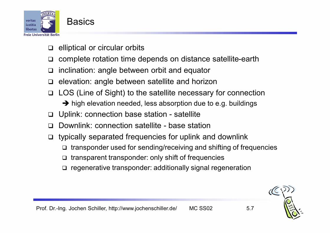
elliptical or circular orbits complete rotation time depends on distance satellite-earth inclination: angle between orbit and equator elevation: angle between satellite and horizon LOS (Line of Sight) to the satellite necessary for connection

high elevation needed, less absorption due to e.g. buildings Uplink: connection base station - satellite Downlink: connection satellite - base station typically separated frequencies for uplink and downlink

transponder used for sending/receiving and shifting of frequencies transparent transponder: only shift of frequencies regenerative transponder: additionally signal regeneration


Inclination

inclination d

d

satellite orbit

perigee

plane of satellite orbit

equatorial plane


Elevation

Elevation:angle e between center of satellite beam and surface

eminimal elevation:elevation needed at leastto communicate with the satellite


Link budget of satellites

Parameters like attenuation or received power determined by four parameters:

sending power gain of sending antenna distance between sender

and receiver gain of receiving antennaProblems varying strength of received signal due to multipath propagation interruptions due to shadowing of signal (no LOS)Possible solutions Link Margin to eliminate variations in signal strength satellite diversity (usage of several visible satellites at the same time)

helps to use less sending power

24

cfrL

L: Lossf: carrier frequencyr: distancec: speed of light


Atmospheric attenuation

Example: satellite systems at 4-6 GHz

elevation of the satellite

5° 10° 20° 30° 40° 50°

Attenuation of the signal in %

10

20

30

40

50

rain absorption

fog absorption

atmospheric absorption

e


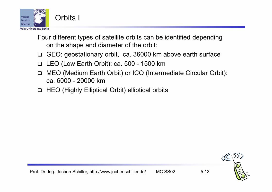
Four different types of satellite orbits can be identified depending on the shape and diameter of the orbit:

GEO: geostationary orbit, ca. 36000 km above earth surface LEO (Low Earth Orbit): ca. 500 - 1500 km MEO (Medium Earth Orbit) or ICO (Intermediate Circular Orbit):

ca. 6000 - 20000 km HEO (Highly Elliptical Orbit) elliptical orbits

Orbits I


Orbits II

earth

km35768

10000

1000

LEO (Globalstar,

Irdium)

HEO

inner and outer VanAllen belts

MEO (ICO)

GEO (Inmarsat)

Van-Allen-Belts:ionized particles2000 - 6000 km and15000 - 30000 kmabove earth surface


Geostationary satellites

Orbit 35,786 km distance to earth surface, orbit in equatorial plane (inclination 0°)

complete rotation exactly one day, satellite is synchronous to earth rotation

fix antenna positions, no adjusting necessary satellites typically have a large footprint (up to 34% of earth surface!),

therefore difficult to reuse frequencies bad elevations in areas with latitude above 60° due to fixed position

above the equator high transmit power needed high latency due to long distance (ca. 275 ms)

not useful for global coverage for small mobile phones and data transmission, typically used for radio and TV transmission


LEO systems

Orbit ca. 500 - 1500 km above earth surface visibility of a satellite ca. 10 - 40 minutes global radio coverage possible latency comparable with terrestrial long distance

connections, ca. 5 - 10 ms smaller footprints, better frequency reuse but now handover necessary from one satellite to another many satellites necessary for global coverage more complex systems due to moving satellites Lower longevity (atmospheric drag, inner Van-Allen-Belt)Examples: Iridium (start 1998, 66 satellites)

Bankruptcy in 2000, deal with US DoD (free use, saving from “deorbiting”)

Globalstar (start 1999, 48 satellites) Not many customers (2001: 44000), low stand-by times for mobiles.

Bankruptcy in 2002. Re-structured in 2004


MEO systems

Orbit ca. 5000 - 12000 km above earth surfacecomparison with LEO systems: slower moving satellites less satellites needed simpler system design for many connections no hand-over needed higher latency, ca. 70 - 80 ms higher sending power needed special antennas for small footprints needed

Example: ICO (Intermediate Circular Orbit, Inmarsat) start ca. 2000

Bankruptcy, planned joint ventures with Teledesic, Ellipso – cancelled again, start planned for 2003. Ended-up deploying one GEO.


Routing

One solution: inter satellite links (ISL) reduced number of gateways needed forward connections or data packets within the satellite network as long

as possible only one uplink and one downlink per direction needed for the

connection of two mobile phones Problems: more complex focusing of antennas between satellites high system complexity due to moving routers higher fuel consumption thus shorter lifetimeIridium and Teledesic planned with ISLOther systems use gateways and additionally terrestrial networks


Localization of mobile stations

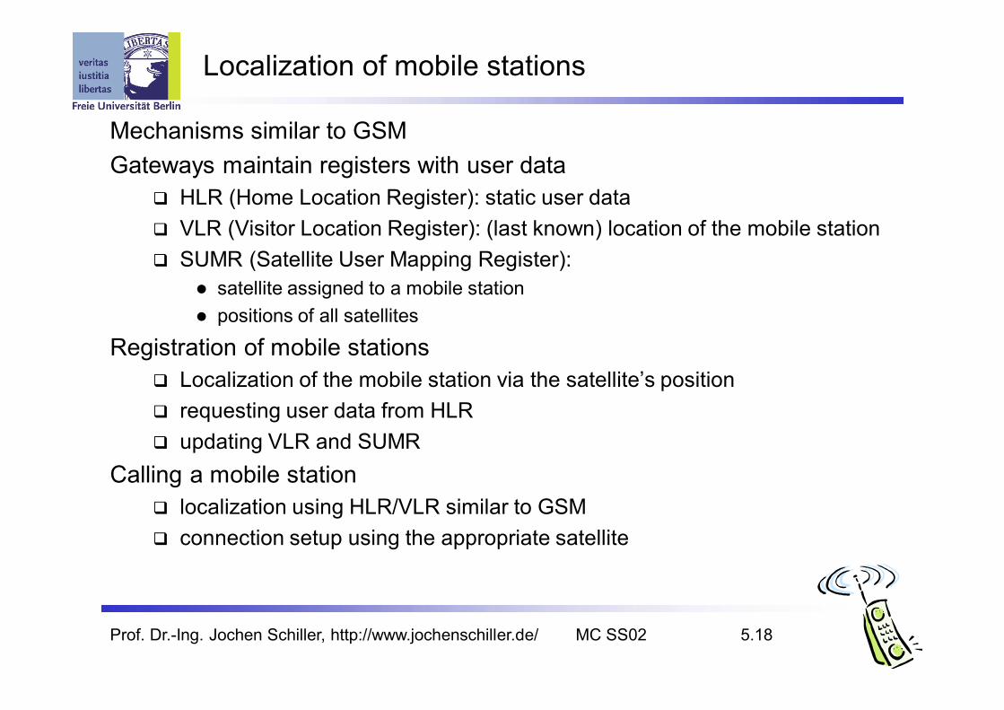
Mechanisms similar to GSMGateways maintain registers with user data

HLR (Home Location Register): static user data VLR (Visitor Location Register): (last known) location of the mobile station SUMR (Satellite User Mapping Register):

satellite assigned to a mobile station positions of all satellites

Registration of mobile stations Localization of the mobile station via the satellite’s position requesting user data from HLR updating VLR and SUMR

Calling a mobile station localization using HLR/VLR similar to GSM connection setup using the appropriate satellite


Handover in satellite systems

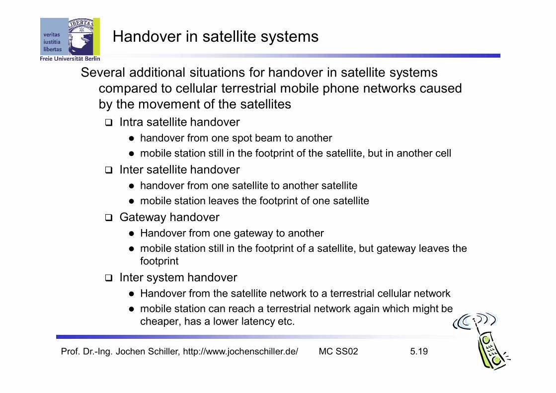
Several additional situations for handover in satellite systems compared to cellular terrestrial mobile phone networks caused by the movement of the satellites Intra satellite handover

handover from one spot beam to another mobile station still in the footprint of the satellite, but in another cell

Inter satellite handover handover from one satellite to another satellite mobile station leaves the footprint of one satellite

Gateway handover Handover from one gateway to another mobile station still in the footprint of a satellite, but gateway leaves the

footprint Inter system handover

Handover from the satellite network to a terrestrial cellular network mobile station can reach a terrestrial network again which might be

cheaper, has a lower latency etc.


Overview of LEO/MEO systems

Iridium Globalstar ICO Teledesic# satellites 66 + 6 48 + 4 10 + 2 288altitude(km)

780 1414 10390 ca. 700

coverage global 70° latitude global globalmin.elevation

8° 20° 20° 40°

frequencies[GHz(circa)]

1.6 MS29.2 19.5 23.3 ISL

1.6 MS 2.5 MS 5.1 6.9

2 MS 2.2 MS 5.2 7

19 28.8 62 ISL

accessmethod

FDMA/TDMA CDMA FDMA/TDMA FDMA/TDMA

ISL yes no no yesbit rate 2.4 kbit/s 9.6 kbit/s 4.8 kbit/s 64 Mbit/s

2/64 Mbit/s # channels 4000 2700 4500 2500Lifetime[years]

5-8 7.5 12 10

costestimation

4.4 B$ 2.9 B$ 4.5 B$ 9 B$


Link Budget

Pr = Pt - 92.4 - 20 Log F(GHz) - 20 Log D(Km) - At + Gt + Gr

G- Gain of antenna t – transmission; r – receptionAt – atmospheric attenuation (dust, rain)

D = 36000 Km -> 20 LogD = 91,1F= 2 GHz -> 20 LogF = 6A=10 dB Gt = Gr = 30 dBiPt = 40 dBm (10 W) -> Pr = - 99,5 dBm


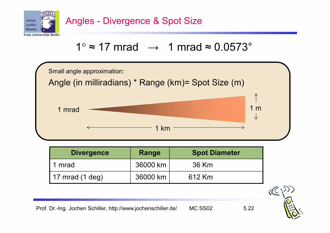
Angles - Divergence & Spot Size

1 mrad

1 km

1 m

Small angle approximation:

Angle (in milliradians) * Range (km)= Spot Size (m)

Divergence Range Spot Diameter1 mrad 36000 km 36 Km

17 mrad (1 deg) 36000 km 612 Km

1° ≈ 17 mrad → 1 mrad ≈ 0.0573°


Antenna Gain vs Divergence

Gain(dBi) = 10 Log (2 / Div) = 10 Log (360º/Divº)

Isotropic Antenna -> Div = 2 / 360º (both Vert. and Hor.) Gain(dBi) = 0

Examples:Div =2º -> Gain(dBi) = 22,6 dBi (2x 22,6 if in both planes)Div =4º -> Gain(dBi) = 19,6 dBiDiv =8º -> Gain(dBi) = 16,6 dBiDiv=12º -> Gain(dBi) = 14,7 dBi (Vert and Hor: 14,7 x 2 = 29,4 dBi)

Nota: a antena da Cisco com Div= 12º tem 21 dBi de ganho, (vs 29.4 dBi teórico) devido a perdas noutras direcções.

Cisco AIR-ANT3338 21dBi Parabolic DishAzimuth 3dB BW =12ºElevation 3dB BW =12º


Received Power based on Antenna Aperture Area (Ae)

Ae = Aphysical * h (h - Antenna efficiency 50%-80%)

Pr = Pt – 10 Log(4 * Footprint / (PI2 *Ae)) – At

Pt = 40dBm (10W)Footprint = 471 716 Km2 (PI x 387.5km x 387.5km) (Iberian peninsula 582 860 km2) Aphy = 1m2 ; h = 50%At = 10 dBPr = 40 – 115.6 -10 = - 85.6 dBm

36000 Km

775 Km1.2º

mobile communications chapter 5: satellite systems · 2019-05-03 · prof. dr.-ing. jochen...

Documents