mobile air conditioning system design study
TRANSCRIPT

Mobile Air Conditioning System Design Study
D. C. Zietlow, J. C. VanderZee, and C. O. Pedersen
ACRCTR-49
For additional information:
Air Conditioning and Refrigeration Center University of Illinois Mechanical & Industrial Engineering Dept. 1206 West Green Street Urbana, IL 61801
(217) 333-3115
September 1993
Prepared as part of ACRC Project 09 Mobile Air Conditioning Systems
C. O. Pedersen. Principal Investigator
....

The Air Conditioning and Refrigeration Center was founded in 1988 with a grant from the estate of Richard W. Kritzer, the founder of Peerless of America Inc. A State of Illinois Technology Challenge Grant helped build the laboratory facilities. The ACRC receives continuing support from the Richard W. Kritzer Endowment and the National Science Foundation. Thefollowing organizations have also become sponsors of the Center.
Acustar Division of Chrysler Allied-Signal, Inc. Amana Refrigeration, Inc. Carrier Corporation Caterpillar, Inc. E. I. du Pont de Nemours & Co. Electric Power Research Institute Ford Motor Company General Electric Company Harrison Division of G M ICI Americas, Inc. Johnson Controls, Inc. Modine Manufacturing Co. Peerless of America, Inc. Environmental Protection Agency U. S. Anny CERL Whirlpool Corporation
For additional information:
Air Conditioning & Refrigeration Center Mechanical & Industrial Engineering Dept. University of Illinois 1206 West Green Street Urbana IL 61801
2173333115

Table of Contents
Page
ABSTRACf .................................................................................. 1
1. INTRODUCTION ............................................................................. 1
2. SYSTEM MODEL ............................................................................. 2
2.1. Recalculation of Compressor Parameters ........................................ 4
2.2. Development of Physically Based Valve Model ................................ 5
2.3. Issues in Equation Solving ........................................................ 7
2.3.1. Newton-Raphson Damping ........................................... 7
2.3.2. Prevalence of the Unknown Variables ............................... 7
2.3.3. Selection of the Unknown Variables ................................. 8
2.3.4. Extent of the Unknown Variables .................................... 8
3. INFLUENCE COEFFICIENTS ............................................................. 9
3. 1. Model Data and Calculations ...................................................... 9
3.2. Influence of Operating Conditions .............................................. 12
3.3. Influence of Design Parameters .................................................. 15
3.3.1. Simulation of Design Changes ...................................... 16
3.3.2. Interpretation of Results .............................................. 16
4. DESIGN OPTIMIZATION EXAMPLE ................................................... 20
4.1. Introduction ........................................................................ 20
4.2. Method .............................................................................. 20
4.2.1. Influence Coefficients ................................................ 20
4.2.2. Finite Changes ......................................................... 22
4.3. Results .............................................................................. 24
APPENDIXA.
APPENDIXB
REFERENCES
CURRENT SYSlEM MODEL ............................................ 28
INDIVIDUAL INFLUENCE COEFFICIENTS ......................... 37
................................................................................. 46
Internal Publications ....................................................................... 46
External Reference ......................................................................... 46


MOBILE AIR CONDITIONING SYSTEM DESIGN STUDY
D.C. Zietlow, J.C. VanderZee and C.O. Pedersen
Department of Mechanical and Industrial Engineering
University of lllinois at Urbana-Champaign, 1993
ABSTRACT This study uses a semi-theoretical steady state computer simulation of an automotive air
conditioning system to evaluate design options. The simulation has been validated with experimental
data. Influence coefficients are used to combine energy and cost data to provide a reasonable basis
for comparison.
Influence coefficients are provided for evaluating seven different design changes. Four of
these are used in an example which illustrates the use of influence coefficients in making design
choices.
For the system modeled it is found that enhancing the internal surface of the condenser coil is
the best option for increasing capacity, increasing efficiency and decreasing head pressure. The other
three design changes included in the example were increasing the condenser length, evaporator length
and compressor displacement.
1. INTRODUCTION One of the intended purposes of the ACRC Project 09 steady state model of a mobile air
conditioning system is identifying aspects of design that significantly affect the system perfonnance.
Design changes can be simulated with the model, and different perfonnance criteria can be examined.
The basic system model is presented in ACRC Technical Report 36. Further modeling
efforts have resulted in improved model accuracy. Chapter 2 presents the current system model and
discusses the improvements made in the compressor and expansion valve components. It also
includes further insights into the modeling process.
Several influence coefficients have been calculated with the system model. First, the
influences of compressor speed in the model are compared to those in measured data. By the
comparisons, the validity of the modeling procedure is established. Then, influences of design
factors (e.g., heat exchanger area, enhancement) in the condenser, compressor, and evaporator are
calculated. By viewing this study from a designer's perspective, it was decided to include the
influence of these factors on cooling capacity, coefficient ofperfonnance (COP), and head pressure.
1

Chapter 3 presents the design sensitivity study. Finally, we demonstrate the use of these influence
coefficients in optimizing the air conditioning system based on cost in Chapter 4.
2. SYSTEM MODEL Improvements have been made on the system model since it was presented in ACRC TR-36.
One of the reasons that the fIrst system model was inaccurate was the compressor performance
deterioration during data collection. Therefore, the compressor parameters were recalculated using
only the data taken before the compressor began to deteriorate.
The fIrst model was incomplete, as well, because it required that the expansion valve pressure
drop be specifIed as an input. The current model uses a semi-theoretical model of the valve based on
the conservation of momentum.
Fig's 2.1 and 2.2 are corrected plots showing the accuracy of the current model for capacity
and COP. Both COP and capacity appear to be modeled quite well by the current model. This model
is complete since only the operational inputs(e.g., compressor speed, air flow rates) of the physical
system must be specifIed as inputs for the model rather than experimental outcomes (e.g., refrigerant
pressure drop).
2

~ u ]
~
! ~ 0 ..... ~ §-u ] .g ::E
Accuracy of COP-Current Model
3
2.5 . . . . .......................... : .......................... ~ ......................... ~ .......................... c- ....................... II ...................... .
~ ! ~ E :: :: :: ::
2 _· .. ············ .. +-.. · .. ·······-1-········· .. _····1 .. ······ .............. ...l ............. _/""" ................. .
1.5
1
~ E E . E .......................... : .......................... '0'......................... . ...................... t:" ......................... ~ ........................ .
i i . i i ..... 111 .................. :.......................... • ................ II.I .. ~I ......................... OOIII.III.I ............ II •• O ..... 111 ... 111 ••• 11 ..... .
E ::::::
~ ~ ~ ~ 0.5
i . ! i i .......................... ······ ........ · .... · .. ·r ............ ········· .. ·r ...... ·· ...... ··········-r···· ............ ······ .. ·r .. · .. ········ .. · .... ···· :: :: :: :: O~~~~~~~~~~~~~~-r~~~~~~~
20
16
12
8
4
o
o 0.5 1 1.5 2
Measured COP
Fig. 2.1. Accuracy of COP-Current Model Accuracy of Capacity-Current Model
. . .
2.5
-_················_·r···_ .... ·· .. ·_·········r·················································:-f···
········_ .. ··············r .. ··················r·_·······............. ························T·····················_···
·· .... ········ .... ···· .... ·····r··············· .. ···· .. · .. · .. · .... ······ .... · .. · ...... ·····r .. · .. ···· .. ·· .... ··· ...... ·· .. r· .. ······· ................. ..
I I I ....... _ ............. _ .... ····· .. ······_ .. T··························r··················_···r················ .. ·······
3
o 4 8 12 16 20
Measured Capacity (kBTU/hr)
Fig. 2.2. Accuracy of Capacity-Current Model
The following sections of this chapter detail the improvements that resulted in the current
model and raise some modeling issues that may merit further investigation.
3

2.1. Recalculation of Compressor Parameters Towards the end of the experimental testing there were signs of compressor deterioration. Oil
was leaking from the compressor and the leakage rate increased as time elapsed. A few months
earlier, when the refrigerant mass flow rate measurements became erratic, a piece of gasket material
was found lodged in the turbine of the flow meter. It is suspected that the material came from the
compressor.
The deterioration is evident from the volumetric efficiency, which should vary systematically
with the compressor speed. The data are calculated directly from experimental measurements and
shown in Fig. 2.3.
>. g Q)
'0 e ~ u 'E
~ ~
0.8
0.7
0.6
0.5
0.4
Compressor Deterioration Based on Experimental Measurements
. . e ; ; ~ Le~d ; ................... .1. ........................................... L .................... r..... .. ............. ; ...................... .1................. .. . 1 ; 01 1 0 jial113-14l1993 ; ; d ; ; ; I I ~ o! -+- ffter Jan t4 .................... + .................. l .................... r .................... l .................. ~ ...................... r .............. · .. ..
.................... t-................ ·t-................ ·t .................. ·t ...................... 1 .................... 1 .................... · I + • t-+-+ I ...................... r .................. · .. t .................. ·1t-.................. + .............. ~ ........ ·+-...... ·t .................. · .. 1 1 + 1 ~ 1 i i 1 i ... i
0.3~~~~~~~~~~~~~~~~~~~~
500 1000 1500 2000 2500 3000 3500 4000
Compressor Speed (rpm)
Fig. 2.3. Compressor Deterioration
The 13 points in the top band are data taken on January 13 and 14, 1993. They demonstrate a
smooth, continuous functional relationship. The remaining points are data taken on January 15th and
later. It is not clear what happened between the 14th and the 15th, but the laboratory records include
some high pressure and temperature alarms. It is clear that after the 14th the compressor efficiency
both decreased and became less consistent. Current compressor equations and coefficients based on
the first 13 points can be found in the FORTRAN residual equations subroutine in Appendix A. The
first version can be found in ACRC TR-36 or ACRC TR-37.
4

2.2. Development of Physically Based Valve Model The fIrst system model used an exact valve model in which the measured pressure drop for
each point was given as input. The current model uses a physically based model to characterize the
performance of the valve. Therefore, experimental pressure drop data is not needed in order to run
the model.
Several theoretically based correlations have been examined to model the valve pressure drop.
Equation. 2.1 is the current equation for the valve model in the system. One even more complicated
and accurate but less theoretically defensible equation was tested. With that more accurate equation,
the system accuracy is not noticeably better, and the range of operating conditions that converges
includes only 12 of the 13 experimental points.
m2 ( C3 ) rn2 ( C5 C6 ) M> = vdi Cl + C2·.1Tsc + rnA + vdo C4 + rnB + vdo (2.1)
where M> is pressure drop, vdi and vdo are inlet and outlet densities, respectively, rh is mass flow rate, .1 T sc is inlet subcooling, and A, B, and C are eight experimentally determined parameters.
5

Figures 2.4 and 2.5 compare the measured system pressures to the modeled pressures. Accuracy of Condenser Inlet Pressure-Current Model
350
'2 310 ..... 00
S
~ 270 00 00
£
_ .......................... ""1" .............................. 1 .. -···· .. ··l··O ... ~ .......... 4- i~··················· .. ··· : : : :
_··························r·····························r---.. · .. ·· ······················ .. ·· .. r····················· 'E 230 ..... .g ~ 190 :::::::::~:=-.= ... :~::::~:::r:::::::::::::::::::::::::::::I::::::::::::::~:~:::I:::::::::::::~:::~::::
150~~~~~~~~·~~~-r· ~~~r'~~~~
150 190 230 270 310 350
Measured Pressure (psia)
Fig. 2.4. Accuracy of Condenser Inlet Pressure-Current Model
Accuracy of Evaporator Outlet Pressure-Current Model
50~~~~~~~-+-r~~~~~r-~~~~
. . . . 45 . . . . .... ··· .. · .. ···· .............. ·r .. · ........ ········· .......... r .. ··········· .... ·· .. · ...... ·r .. · .. · .. ········ .... · ·· .... r ........ ·· .. · .. · ............ · : : : : E E . E
~ ~ . ~ ............................... : ................................ : .............. ...... •••• .. ··~.·· ••• • .... ••••• ............... oco •••••••••••••• ••••••••••••••••
I ! I I 40
35 ............................. .J.... . ............... G··r-·························/····················· .. ········1··················· .. ·· .. ··· 0000 ; ; ;
O! ! ! ! ! !
30~~--~~~~-r~~--r-~-+-+------~
30 34 38 42 46 50
Measured Pressure (psia)
Fig. 2.5. Accuracy of Evaporator Outlet Pressure-Current Model
6

The valve model has a root-mean-square error of over 10 psi, so the visible error is expected.
A more sophisticated valve model might provide greater accuracy, but the current system model
already has good accuracy for heat transfer modeling and should predict correctly the influence of
various factors on the pressures.
2.3. Issues in Equation Solving Several aspects of the solution process have been considered during the development of the
mobile air conditioning system model. ACRC TR-36 mentions some of them briefly. Further
comments on the method of solution are collected in this section.
A Newton-Raphson method is used to solve the model equations. This method numerically
finds the derivatives of each residual equation with respect to each unknown, thus finding a
linearized system about the initial values. That linearized system is solved exactly by linear algebra to
calculate the next values. Unless the actual system is linear, iteration is required until the residuals
are sufficiently small. Even univariate functions can be selected that fail in this method even with
fairly accurate initial values.
2.3.1. Newton-Raphson Damping One modification to the implementation of the method is that it is damped by 50% on the first
iteration, that is, the second values are selected between the initial guesses and the first linearized
solution. This is useful primarily because this system of equations uses refrigerant property routines
that are discontinuous across the saturation dome. When values change too drastically, the
assumptions about refrigerant states around the loop can be violated.
More general issues center on the design of the residual equations themselves. Three of them
addressed below are called, for the purpose of this report, the prevalence, selection, and extent of
the unknowns.
2.3.2. Prevalence of the Unknown Variables The prevalence of the unknowns is simply the number of them. Early models were solved in
the Engineering Equation Solver (EES) program. Every variable, unless it is contained in a function
or can be algebraically solved initially, is treated as an unknown by EES. An EES version of the
system model could have hundreds of variables. As reported in ACRC TR-36, the number of
unknowns in the FORTRAN model has been reduced to 16, fewer than the sum of those in the
component models.
One benefit of a reduced number of variables is the reduction in computation and thus
increased speed of solution. Increased stability can also be expected, because equations that embody
knowledge of the system are being used as constraints instead of residual equations.
7

2.3.3. Selection of the Unknown Variables Selection of unknowns involves choices after the number of equations has been determined.
First, by the ordering of the equations, different variables can be eliminated or left as unknowns.
Also, the same variable can be found in different ways. For example, a pressure can be an unknown
itself, be found as an unknown pressure drop from another pressure in the system, or be a saturation
pressure for some unknown temperature.
Careful selection can result in useful, physically-based unknowns. Such variables allow
simple derivation of accurate initial guesses and variable bounds, and they are easily interpreted to
gain understanding of the solution process. Selection of unknowns seems to affect convergence, as
well.
2.3.4. Extent of the Unknown Variables The extent of the unknowns has to do with how often the unknowns are used in the model
equations. An example of this issue is the condenser outlet pressure in this system model. One of the
unknowns is the condenser pressure drop, and that is compared to the condenser model pressure
drop equations in one of the residual equations. The condenser outlet pressure also appears in the
expansion valve equations. The extent of the unknown is greater if the unknown pressure drop rather
than the result of the condenser equations is used to determine this outlet pressure.
The most striking example of an unknown with variable extent is the refrigerant mass flow
rate. That was an unknown in an early version of the system model. The compressor is the fIrst
component treated in the system, and the compressor equations provide a calculated mass flow rate.
Either of these could be used for all the succeeding components. Perhaps unknowns of truly variable
extent can always be eliminated. The condenser pressure equations require the density calculated
from the outlet pressure, so that unknown must be included; however, it does therefore influence the
calculated pressure drop and extend indirectly when the calculated value is substituted.
Limiting the extent of the unknowns might be considered as performing steps of a successive
substitution within each Newton-Raphson step. Since order of substitution is of critical importance in
successive substitution, the order of evaluation in the residuals block must be important in
determining the benefIt of substituting calculated values there.
8

3. INFLUENCE COEFFICIENTS Design infonnation can be obtained from the model by simulating design changes instead of
constructing and testing many prototypes. This study presents infonnation in the fonn of influence
coefficients. An influence coefficient is a ratio of the effect on one variable to the exclusive small
change in another variable. For this report, the influence coefficient represents the influence of design
variables (e.g., heat exchanger length and heat transfer enhancement) upon system performance
variables (e.g., coefficient ofperfonnance and capacity)
This study ftrst calculates influence coefficients for compressor speed, an operating
condition. Since compressor speed varies in the experimental data, the simulation results are
compared to the experimental results to further validate the model accuracy and calculation of
influence coefficients. Then design changes in the condenser, compressor, and evaporator are
simulated. An example is presented in chapter four to demonstrate how these influence coefficients
can be used for guiding design efforts.
3.1. Model Data and Calculations Convenient input data are used for the simulation to produce organized results for plotting.
Figures 3.1 and 3.2 show the two primary data sets.
9

Inlet Air Temperature
to Evaporator (OF)
120
100
§ 8 N ~ ~ §
Speed of Compressor N
(rpm)
Values of Other Operating Variables: Barometric Pressure=14.4 psia
Air Flow Rate through Condenser=37oo CFM Inlet Air Temperature to Condenser=85 of Inlet Humidty Ratio to Condenser=.005 Inlet Humidity Ratio to Evaporator=.01
Ambient Temperature=80 of
Air Flow Rate Through
Evaporator (CFM)
Figure 3.1. Simulation Data Set A with Evaporator Side Variations
10

100
2000 2500 3000
2000
Speed of Compressor (rpm) 3000
Values of Other Operating Variables: Barometric Pressure=14.4 psia
Air Flow Rate through Evaporator=700 CFM Inlet Air Temperature to Evaporator=110 of
Inlet Humidty Ratio to Condenser=.005 Inlet Humidity Ratio to Evaporator=.01
Ambient Temperature=80 of
Air Flow Rate Through
Condenser (CFM)
Figure 3.2. Simulation Data Set B with Condenser Side Variations
Figure 3.1, input set A, has three values for evaporator air flow rate and two for temperature
in almost all possible combinations. One combination is absent because it is outside the region of
convergence for the modeL Figure 3.2, input set B, has three values for condenser air flow rate and
two for temperature in all possible combinations. Both data sets have three values for compressor
speed. The remaining operating variables remain constant at average values throughout the
simulation.
11

Simulated output provides a prediction of system perfonnance; these predicted values are as
accurate as the model. To calculate the influence of each parameter, the complete input sets are
simulated with a change in that parameter. Compressor speed is changed by changing the input
values. Design factors are changed by altering the appropriate parameters in the residual equations of
the model.
One convenient fonn of influence coefficient is a dimensionless ratio of the percentage change
in effect to the percentage change in cause. Most of the simulation changes are 1 % increases in
design variable (the independent variable) so that the resulting percentage change in the performance
variable (the dependent variable) is the influence coefficient. Equation 3.1 uses coefficient of
performance, COP, and compressor speed in rpm, to show an example of a definition of this type of
influence coefficient (I.C.) The subscripted variables are the original values from the unchanged
input data.
%~COP I.C.= %&-pm
(COP 0 -COP) rpm 0
COP 0 rpmo -rpm
3.2. Influence of Operating Conditions
(3.1)
The only operating condition influence studied is compressor speed. The primary motivation
for studying the influence of operating conditions on the perfonnance variables is for model
validation. The model was validated for function values in Chapter 2. This validation looks at the
ability of the model to predict derivative values (influence coefficients). Since operating variables
were changed, during the experimental testing, the actual experimental influence coefficients can be
calculated and compared with the model's predictions. The input data is the same as that shown in
Figure 3.1 where the evaporator's operating conditions are varied. Figures 3.3 and 3.4 show the
calculated effects on system COP and capacity of increasing speed by 1 %. As might be expected, the
influence on COP is negative and on capacity is positive.
12

Influence of Compressor Speed on COP
-0.58 o 5OO1b~evap.arr x 700 Ib~ evap. air .................... J; ................... --r ............. ······r·······~··· b. 900 Ib~ evap. arr
~ j j x. . .
I] -~r~:I~jl:: , I I ~ I I ~
······················,······················r····· .............. -r .................... "1" .................... -r ..................... !"" ................... .
: ; ; b.; ; ~ ..................... ~...... evap. arr Tin .............. evap. arr flow rate .. j ..................... .
I (100 & 120 OF) r -0.7~~~~~~~~~~~~~~~~-r~~+
-0.6
13 -0.62 8-en
~ - -0.64 -~ u -0.66 ~
-0.68
1800 2000 2200 2400 2600 2800 3000 3200
Compressor Speed (rpm)
Fig. 3.3. Influence of Compressor Speed on COP
Influence of Compressor Speed on Capacity
0.22
0.2
] 0.18 0.. en
0.16 ~ -- 0.14 a .... ~ 0.12 ~ u
0.1 ~
0.08
0.06 1800 2000 2200 2400 2600 2800 3000 3200
Compressor Speed (rpm)
Fig. 3.4. Influence of Compressor Speed on Capacity
13

The previous graphs illustrate the variation in influence the compressor speed has upon the
performance variables as the evaporator operates through its entire range.
To calculate the experimental influence coefficients data points were selected where the
evaporator air flow rate was held constant at around 700 lbm/hr. They are shown in Figure 3.5 with
a curve fit that accurately gives COP as a function of compressor speed. These points were selected
from the set of data which was taken prior to the deterioration of the compressor.
Measured COP as Function of Compressor Speed
3~~~~~~~~~~~~~~~~~~~~~~
2.5 ... ····················r························l·························r························r·························r························
2 .......................... : ....................... .1. ........................ .1 ......................... .1 ......................... .1. ........................ .
-1;--~--1-I---1.5
! ! ! 11-~~~~~~~~~~~~~~~~~~~~
1000 1500 2000 2500 3000 3500 4000
Compressor Speed (rpm)
Fig. 3.5. Measure COP as Function of Compressor Speed
The curve fit is needed because influence coefficients are calculated for small changes in the
independent variable and the experimental changes were fairly large. The equation of the curve is
given by Equation 3.2. By taking the derivative, Equation 3.3 is found, which allows the calculation
of the influence coefficient by Equation 3.4. The exact ratio of rpm to COP from the measured data is
used in this equation. Equation 3.4 corresponds to Equation 3.1 if the partial derivative is changed to
a fmite difference.
COP = 153.4 . (rpm) -0.58804
OCOP 88 drpm = 153.4· (-0.58804) . (rpm) -1.5 04
I C _..!P!!!.. acop .. - COP drpm
14
(3.2)
(3.3)
(3.4)

Fig. 3.6 shows the influence coefficients calculated for COP by the above equations for the
experimental data and compares them with the model results. The model used experimental data for
its inputs rather than the simulation data sets.
Influence of Compressor Speed on COP
-0.56
-0.58
1 -0.6 en ~ -0.62
¢ . ¢ . ¢ i
·=:l···r·~:··~=t:Jr: i :k iii i
··········----····---·i-···-··-·-·----·----·-~-··-···················i···········--······---.t----··········· ........ ~ ...... -............... { ..... --........ ---.--. i * i ~ i i --Po. -0.64
0 u ~ -0.66
-0.68
j j j j ~ j ······················i······················1·······················?····------············t······················r···---···········--···i······················
1 j ! l 1 l iii i )/: i ---.-...... --......... ~-.-........... ----.. -."-.-.-....... _-_._-_ .... , .............. __ .. __ .................. ·········f······ __ ··············I······················
i 0 experimental data fit i ~ .. ····· .. ········ .. t········· x model run · .. '1" .... · .. ··· ........ ·1 ...... ·· .......... · ..
-0.7~~~~; ~~~~~~~~~~~;~~~; ~~+
500 1000 1500 2000 2500 3000 3500 4000
Compressor Speed (rpm)
Fig. 3.6. Comparison of Experimental and Model Influence Coefficients
The results agree to within 10 percent for the midrange of the compressor's operating
envelope but diverge at the extremes. The model can be used to predict the influence coefficients of
operating variables within a reasonable range of operating conditions. We expect the model to also
predict the influence of design changes accurately.
3.3. Influence of Design Parameters Unfortunately, the designer does not have control over many of the operating variables.
These variables are normally a constraint of the system. A much more interesting exploration is the
influence of design variables upon the performance of the system. Examples from the second data
set, in which the inputs to the condenser were varied, are included in Appendix B. Figures B.l-B. 8
show results for factors affecting condenser design. Figures B.9 - B.12 show results for the
compressor. Figures B.13 - B.16 show results for the evaporator. These data are provided so that
analysis can be performed without again running the model. The next section describes the changes
made in the residual equations for simulating the design changes studied.
15
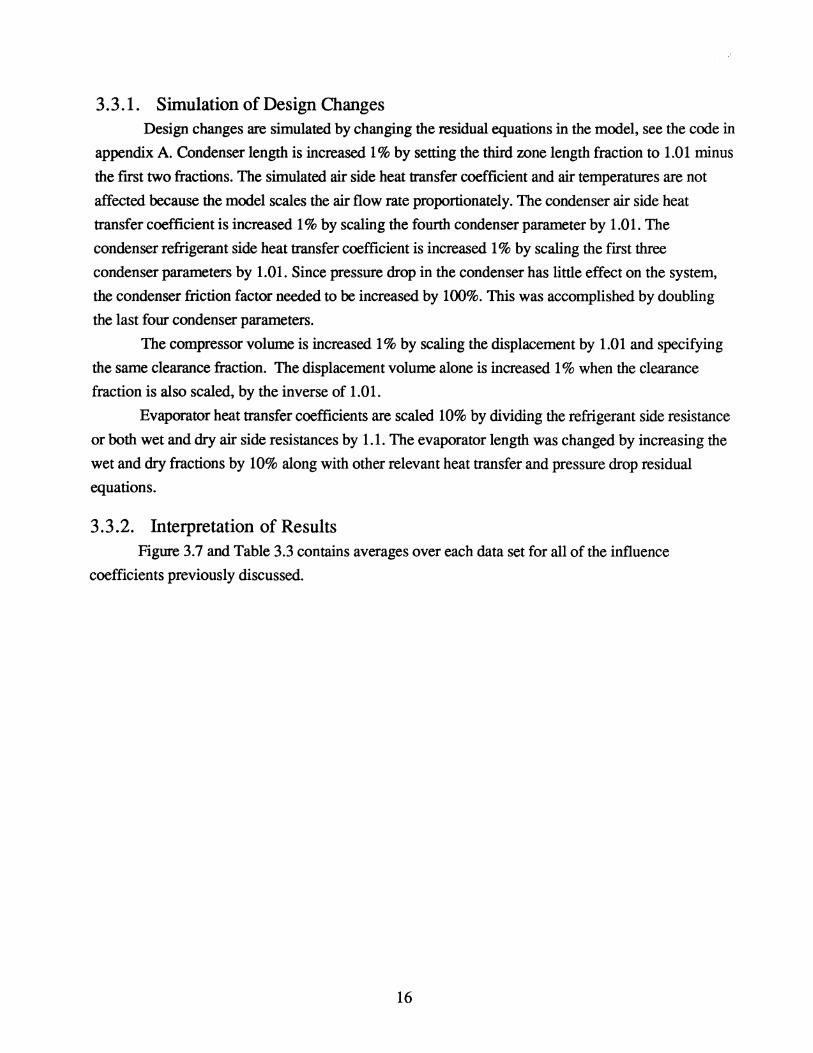
3.3.1. Simulation of Design Changes Design changes are simulated by changing the residual equations in the model, see the code in
appendix A. Condenser length is increased 1 % by setting the third zone length fraction to 1.01 minus
the fIrst two fractions. The simulated air side heat transfer coeffIcient and air temperatures are not
affected because the model scales the air flow rate proportionately. The condenser air side heat
transfer coeffIcient is increased 1 % by scaling the fourth condenser parameter by 1.01. The
condenser refrigerant side heat transfer coeffIcient is increased 1 % by scaling the first three
condenser parameters by 1.01. Since pressure drop in the condenser has little effect on the system,
the condenser friction factor needed to be increased by 100%. This was accomplished by doubling
the last four condenser parameters.
The compressor volume is increased 1 % by scaling the displacement by 1.01 and specifying
the same clearance fraction. The displacement volume alone is increased 1 % when the clearance
fraction is also scaled, by the inverse of 1.01.
Evaporator heat transfer coefficients are scaled 10% by dividing the refrigerant side resistance
or both wet and dry air side resistances by 1.1. The evaporator length was changed by increasing the
wet and dry fractions by 10% along with other relevant heat transfer and pressure drop residual
equations.
3.3.2. Interpretation of Results Figure 3.7 and Table 3.3 contains averages over each data set for all of the influence
coefficients previously discussed.
16

Summary of Average Influence Coefficients
0.6 0.4 0.2
O-tCIII~ Influence -0.2
Coefficien' -0.4 -0.6 -0.8
-1
~d~.El<l= uuu~~ trl cd
~~ Influencing Facto -
Performa nCE Variable
Figure 3.7 Summary of Average Influence Coefficients
17

KS Ehr
ress.-A -B
Influencin Factor
Table 3.3. Summary of Average Influence Coefficients
Only the first fIfteen points of set A are included in the averages because the last two points
tended to be extreme. Although the graphs present more information, the summary table is
convenient for comparing the effects of different operating and design factors. Influence on COP,
capacity, and head pressure are reported in the table. Together these two data sets represent a
reasonable operating range of the air conditioning system. Under the assumption that the air
conditioning system operates under each of these conditions for an equal amount of time over the life
of the system, these numbers represent the influence of the design change on the performance
variable for the life of the system. Weighting factors can be used in conjunction with the data in
Appendix B to evaluate conditions which differ from this assumption.
From a purely energy standpoint, the condenser length is the most promising to improve all
measures of perfonnance. The fIgures show, also, that the influence is less at higher condenser air
flow rates, but on average, a 10% increase in condenser size improves COP around 5%, capacity
around 2%, and decreases head pressure around 8%.
One might consider using enhanced condenser tubes with both a higher heat transfer
coeffIcient and a higher pressure drop. The table shows that in order to maintain or reduce the head
pressure, the heat transfer improvement must be at least 1.5% per multiple of pressure drop increase.
18

A 15% increase in heat transfer coefficient with a factor of 10 increase in friction factor would
improve capacity around 1 % and COP over 1.5%.
Increased compressor displacement has effects similar to operating at a higher compressor
speed. The same increase in capacity is achieved with smaller decrease in COP and smaller increase
in head pressure by increasing displacement, however. The compressor simulation assumed the same
rate of heat loss and same efficiencies at the larger size.
Evaporator heat transfer coefficients do not leave as much room for improvement, but the
data do show that improvements an the air side are four times as effective. It is interesting that at the
lower evaporator air flow rates, the improved evaporator heat transfer tended to have a greater,
though still small effect of increasing head pressure.
19

4. DESIGN OPTIMIZATION EXAMPLE
4.1. Introduction In Chapter 3 we evaluated the design options based strictly on energy criteria. This is an
inadequate measure of the feasibility of a design change. It is important to look at the cost to
implement each measure. If increasing the length of the condenser increases the capacity by twice as
much as enhancing the tubes then from an energy standpoint it is the best option. But if it costs four
times as much to increase length as to enhance the tubes then the tube enhancement becomes the best
option.
This next section demonstrates how cost information can be integrated with the influence
coefficients calculated in the previous chapter to evaluate design choices. One of the objectives of a
manufacturer of air conditioning systems for automotive applications is to increase the cooling
capacity. This will reduce the time to reach comfort when the vehicle is first used. First, the least
costly way to increase the capacity of the system is determined. Then the same method is applied to
finding the least costly way to reduce head pressure (the pressure at the outlet of the compressor) and
increase the coefficient of performance.
4.2. Method
4.2.1. Influence Coefficients To use the influence coefficients from the previous section we need to put cost information in
a form which can be used. Below is the general form used to apply the cost information. ~design variable
~cost (4.1)
For small changes in the design variable Equation 4.1 becomes ddesign variable
dcost (4.2)
If this is then multiplied by the influence coefficient of interest, the influence of cost on
capacity can be determined as follows in Equation 4.3:
acapacity
acost
acapacity
adesign variable
adesign variable
acost (4.3)
When this is done for several different design variables a comparison can be made to find out
which change in design variable has the most effect on increasing the capacity at the lowest cost.
The following design variables were evaluated for this example.
20

1) Replace smooth tubes with microfm tubes in the condenser
2) Increase the length of the evaporator
3) Increase the displacement of the compressor
4) Increase the length of the condenser
Below are the relevant specifications of the air conditioning system tested in this study.
1) Evaporator length (refrigerant path): 3.6 m
2) Weight of evaporator plates and fins: 1.04 lb/m
3) Evaporator material: aluminum
4) Compressor displacement volume: 170 cc
5) Condenser length (refrigerant path): 30 m
6) Weight of condenser tubing: .411b/m (ASHRAE 1992 Systems Handbook)
7) Weight of condenser fins: .41Ib/m (estimated)
8) Condenser material: aluminum
Cost data were obtained from various members of the Industrial Advisory Board. These
figures are current but should be modified for your particular application. This modification is made
by following the method described above in Equations 4.1 through 4.3. The cost figures are
incremental, not average, costs. It is the cost for adding the design change assuming the fixed costs
for setting up the production line would be the same even if the design change were not implemented.
Table 4.1 shows the cost figures used for this example along with the corresponding change in the
design variable.
T bl 41In alCh a e . crement dC ·De· V·bl angesan ostsm SIgn ana es
Design change Change in design variable Incremental Cost
Enhance condenser tubes ahr=I00%(Eckels, 1991) $.40/lb
M7=100%(Eckels, 1991)
Increase evaporator len$h aEL=10% $.95/lb
Increase compressor Mm=lO% $2.50
displacement
Increase condenser length aCL=lO% $. 95/lb
where, hr-heat transfer coefficient on the refrigerant side
Pr-pressure drop on the refrigerant side
A word should be added about the assumptions which were made to determine the changes in
heat transfer coefficient and pressure drop by enhancing the condenser tubes. The work by
Eckels(I991) shows the heat transfer coefficient improves by 75 to 150% and the pressure drop
increase was less this. For this analysis it was assumed that the pressure drop increase was the same
as the improvement in the heat transfer coefficient. This adds a slight penalty to the enhancement
design option since an increase in pressure drop decreases the capacity. The actual calculation of the
21

influence of enhancement on the capacity was made up of two components (the influence of heat
transfer coefficient and pressure drop on capacity) which were added together and then used in
equation 4.3
The previous cost data were used to construct influence coefficients of the influence of cost
on the design variable, the rightmost factor in Equation 4.3. These are contained in Table 4.2.
T bl 4 2 Infl f C th De' V' bl a e . uenceo oston e Slgn ana es
Design Variable Influence Coefficient
ddesign variable(% )/Ckost($)
Enhance condenser tubes 96
Increase evaporator length 26
Increase compressor displacement 4.2
Increase condenser length 4.5
4.2.2. Finite Changes Influence coefficients work well in evaluating changes if they are relatively small. If the
change in a design variable is relatively large then influence coefficients begin to lose their
effectiveness. The reason for this is that an influence coefficient is the slope of a curve at a point.
When it is applied one assumes that this slope is constant over the range of interest. If the curve is
nonlinear and the range is large, the error can become significant. This is illustrated below in Figure
4.1.
22

» .... • - roo..
~.E. a~ 8~ ~o .... 0 00 ~,...; >'-' ~
Prediction Using Influence Coefficients 24 ~~~~~~~~~~~~~~~~~~+-~~~
22
20
18
16
. . . . . ······· .. ··············r······················r······················r·····················T···· ·················r······················
I I I I
rf-'rr ·······················t·················· ··t······················~·······················t······················9·······················
I r ! ! ! . : : : :
j 1 l ! . ! : : : ················o···-r·······················r·····················"j·······················r················ ...... ]"" ..................... .
o Actual Model Capacity
--Predicted Capacity Using
14 ···············_······r················ Influence Coefficient
12 4-~~~~~~~~~~~~~~~~~~~~~
o 100 200 300 400
Scaling of the Refrigerant Side Heat Transfer Coefficient in Condenser
(%)
500
Figure 4.1. Error from Using Influence Coefficients
600
This graph was generated by scaling the appropriate parameters in the condenser model to
simulate an change in the refrigerant side heat transfer coefficient. The influence coefficient was
calculated at the baseline condition (scaling factor = 100%) and was used to predict the effect of
changes in the refrigerant side heat transfer coefficient on the evaporator capacity. The error between
the prediction and the model results is small for small changes in the design variable but increases
significantly for large changes.
23

4.3. Results The influence coefficient for the four design changes under consideration were calculated using
Equation 4.3. The results are displayed in the Figure 4.2.
12
10
8
6
4
2
o
Influence of Design Changes on Capacity
e f ra ~
DeSIgn Change
M ... o s:: Vl Q)
~ E M Q) 0.. u E ~ rq e-
Figure 4.2. Influence of Design Changes on Capacity Using Influence Coefficients
This shows that for small changes in the design variables, enhancing the condenser tubes is
the most cost effective option for increasing the evaporator capacity for the system tested. One of the
biggest problems members of the Industrial Advisory Board say they face is rmding enough space to
install the heat exchangers. One recommendation based on these results is that the condenser and
evaporator lengths be reduced to conserve space. It is possible to do this, if the condenser tubes are
enhanced at the same time, without degrading the capacity of the evaporator.
24
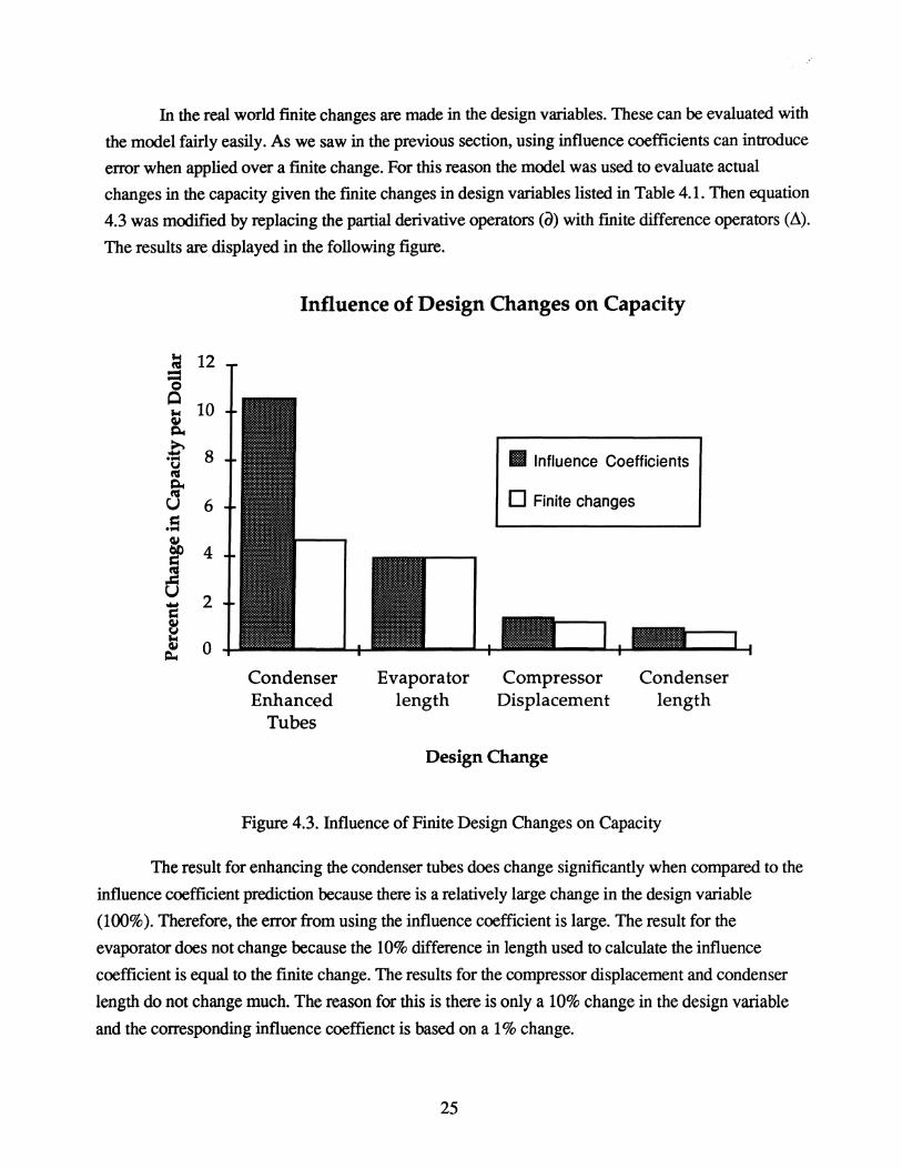
In the real world finite changes are made in the design variables. These can be evaluated with
the model fairly easily. As we saw in the previous section, using influence coefficients can introduce
error when applied over a fmite change. For this reason the model was used to evaluate actual
changes in the capacity given the fmite changes in design variables listed in Table 4.1. Then equation
4.3 was modified by replacing the partial derivative operators (a) with fmite difference operators (L\).
The results are displayed in the following figure.
~ !U --0 0 ~ QJ ~
.e-. .-v !U ~ !U U .5 QJ
ff .2 u d QJ V ~ QJ ~
12
10
8
6
4
2
0
Influence of Design Changes on Capacity
Condenser Enhanced
Tubes
III Influence Coefficients
Evaporator length
o Finite changes
Compressor Displacement
Design Change
Condenser length
Figure 4.3. Influence of Finite Design Changes on Capacity
The result for enhancing the condenser tubes does change significantly when compared to the
influence coefficient prediction because there is a relatively large change in the design variable
(100%). Therefore, the error from using the influence coefficient is large. The result for the
evaporator does not change because the 10% difference in length used to calculate the influence
coefficient is equal to the finite change. The results for the compressor displacement and condenser
length do not change much. The reason for this is there is only a 10% change in the design variable
and the corresponding influence coeffienct is based on a 1 % change.
25

The overall conclusion from this example is, however, the same. Adding enhanced tubes to
the condenser is the least expensive way to increase the capacity of the system. With more capacity
the time to reach comfort in the passenger compartment will be reduced. This conclusion is only
applicable to the system and set of operating conditions used for this study. To do a similar study for
other systems, new parameters should be developed for those systems.
Although capacity is an important performance variable, the other two performance variables
are also useful. The influence coefficient for the coefficient of performance tells which design
variable improves the system efficiency for the least cost. The influence coefficient for head
pressure(the refrigerant pressure at the outlet of the compressor) is important since Rl34a is a higher
pressure refrigerant. Figure 4.4 displays influence coefficients for all three perfonnance variables
based on finite changes in the design variables.
Influence Coefficient (% change in performance variablel$)
Design Variable
Influence of Design Changes Based on Finite Changes in DeSign Variables
J -8 c:
COP Capacity
Head Pressure Performance
Variable
Figure 4 4. Influence of Design Changes on Three Performance Variables
This figure shows enhancing the tubes of the condenser is the best option for all three performance
variables. It produces the largest increase in both capacity and COP for each dollar of investment. It
also produces the largest decrease in head pressure.
26

5. CONCLUSIONS From this study the following conclusions can be drawn.
1) The computer simulation has been validated with experimental data. It models the capacity,
coefficient ofperformance(COP), pressures, and the influence of compressor speed on COP
accurately.
2) Influence coefficients can be used to rank design options when small changes are made in the
design variables. The simulation should be used to model large changes in the design variables.
3) For the air conditioning system studied, enhancing the condenser tubes is the best alternative to
increase capacity and COP and lower head pressure. The other three design variables studied were
increasing condenser or evaporator lengths and compressor displacement.
4) Cost analysis, as opposed to energy analysis alone, provides a better basis of comparison among
design options. From an energy standpoint alone, increasing the condenser length would be the
best option.However, the cost analysis found enhanced tubes to be the best option since it is less
expensive to implement.
27

APPENDIX A. CURRENT SYSTEM MODEL
C University of illinois at Urbana-Champaign
C Department of Mechanical and Industrial Engineering
C ACRC Project 09
C
C 1993 by Joel VanderZee
C
C This routine must be linked with refrigerant property routines.
Subroutine sysresid(input,out,resids)
double precision hundred,unity,zero,negone,pi,Hair,third
double precision input(1O),out(16),resids(16)
C** accumulator and acc.-comp. ref. line
double precision acl,ac2,aR(2)
double precision Pdrop,arpo,atsat,arh
C** compressor
double precision kparm(8),kR(I),ktsat
double precision krpi,krhi,hrpo,rpm,kTamb,mr,power,krho
double precision krsi,krri,krhos,krros,krti
double precision V disp,Kcl, ClearEff, V doCS, VolEff, V dot
double precision workc, workcs,IsenEff,kQ,krdh,xx,yy ,zz
C** comp.-cond. ref. line
double precision krpo
double precision crpi,krro,kcdp
C** condenser
double precision cparm(9),cR(7),calcpo
double precision cK,D,A,m,cMa,cHumRat
double precision crti,crhi,crdi,crp 1 ,crt 1 ,crh 1 ,crdl
double precision crp2,crt2,crh2,crd2,crpo,crto,crho,crdo
double precision cati,cato_sh,cato_c,cato_sc
double precision cahi,caho_sh,caho3,caho_sc
double precision Tbar,Tabar,UA,FF,Q,Qa,Qcalc,DP,DPcalc
double precision shfrac,cfrac,scfrac,UA1,UA2,FF1,FF2,DP1,DP2
28

C** expansion valve
double precision xp(8),xdrop,xR(I),ctsat,subcool
C** evaporator
double precision epann(1O),eR(5)
double precision pamb,Rflow ,Eaflow ,Erpi,Erhi,Eawi,Eati
double precision Erpo,Tsur,Qad,Qaw,hab,Erho,Eawo
double precision fd,rr,rm,rad,raw
double precision Erti,Erto,Eahi,Eaho,Erdi,Erdo,Erxi
double precision hasurw ,hasurd, wasurw, wasurd
hundred = 100.0
unity = 1.0
zero =0.0
negone = -1.0
pi = 3.141592653589793
third = 1.0/3.0
C** compressor
kTamb = input(8)
rpm = input(9)
krpi = out(2)
Call Fsatp(krpi,ktsat,xx,yy)
krti = ktsat + out(l)
krpo = out(3)
krho = out( 4)
xx = hundred
Call Mixptq(krpi,krti,xx,krri,krhi,krsi)
C ref. density (lb/ft"3)
C suction entropy (Btullb-R)
C for mass flow rate:
kpann(l) = 0.682718
kpann(2) = -1.017ge-4
C (rpm"-I)
kpann(8) = 0.11761
29

C (lb/ftA3)
C for isen. eff.:
kpann(3) = 0.758856
kpann(4) = -7.00616e-5
C (rpmA-l)
kpann(5) = 0.0070387
C (lb/ftA3)
C for heat loss:
kpann( 6) = 26.74
C (Btu/rpm-hr)
kpann(7) = 15.32
C (B tu/hr-F)
C Vcl =0.243
C clearance vol (in.A3)
V disp = 10.37
C displacement (in.A3)
C Kcl = VcWdisp
Kcl = 0.243/10.37
C clearance fraction
Call Mixsp(krsi,krpo,xx,krhos,krros,yy)
C discharge enth. at const. ent. (BTU/lb)
C discharge density at const. ent. (lb/ftA3)
ClearEff = 1 - Kcl * (krros/krri - 1)
C clearance volum. eff.
V doCS = ClearEff*rpm*V disp/1728
C isen. volum. flow rate (cfm)
VolEff = kpann(1) + kpann(2)*rpm + kpann(8)/krri
C isen. volum. eff.
C NOTE! Called this "effrat" in analyzer!!
C It is NOT the SAME as the "voleff' there!!
V dot = VolEff*V doCS
C suction ref. volumetric flow rate (cfm)
C kR(1) = mr - Vdot*60*krri
mr = V dot*60*krri
C ref. mass flow rate (lbm/hr)
30

workcs = krhos - krhi
C isen. work (BTU/lb)
IsenEff = kpann(3) + kpann(4)*rpm + kpann(5)/krri
C isen. eff.
workc = workcs/lsenEff
C actual work compo
C kR(2) = (power - mr*workc)/12000
power = mr*workc
C required compo power (divide by 12,000 to norm.)
kQ = kpann(6)*rpm**0.5 + kpann(7)*(kTamb-krti)
C heat loss
krdh = (power - kQ)/mr
C enth. rise
kR(1) = krho - (krdh + krhi)
C compo discharge ref. enth.
C** comp.-cond. ref. line
kcdp = 6.285674e-4
C empirical pressure drop coefficient (hr"2-ftA3-psi/lbA3)
crhi = krho
C no heat transfer
Call Mixhp(krho,krpo,xx,yy,krro,zz)
crpi = krpo - kcdp*(mr**2)/krro
C pressure drop
C** condenser
C for heat transfer:
cpann(l) = 0.1632045994812011
cpann(2) = 5.2751165442019870E-02
cpann(3) = 0.2198721449019462
C (ftA2-F-hr-lbAO.8/BTU-hrAO.8)
cpann(4) = 0.2831501216515262
C (ftA2-F-hr-lbAO.67/BTU-hrAQ.67)
C for pressure drop:
31

cpann(5) = 2.914678168647671
cpann(6) = 0.4834631486447542
cpann(7) = -0.7516406390569577
C (1h"0.25/hr"0.25)
cpann(8) = 8.20520338402oo130E-02
C (-)
cK = 1.66546E-ll
C this above to convert Ihm-ft/ft"2-hr"2 to psi
D =0.02083
C (ft)
A = pi*D**2/4
C (ft"2)
m=mr
cMa = input(2)
cati = input(3)
cato_sh = out(7)
cato_c = out(8)
cato_sc = out(9)
cHumRat = input(4)
cahi = Hair(cati,cHumRat)
caho_sh = Hair(cato_sh,cHumRat)
caho_c = Hair(cato_c,cHumRat)
caho_sc = Hair(cato_sc,cHumRat)
Call Mixhp( crhi,crpi,crti,xx,crdi,yy)
crpl = crpi - out(lO)
crp2 = crpi - out(ll)
crtl = 0
Call Mixptq( crp 1 ,crt 1, unity ,crd 1 ,crh 1 ,xx)
crt2 =0
Call Mixptq( crp2,crt2,zero,crd2,crh2,xx)
crpo = crpi - out(l2)
crto = crt2 - out(13)
xx =negone
Call Mixptq( crpo,crto,xx,crdo,crho,yy)
32

Q = m*(crhi - crhl)
VA = 2/(cparm(4)!cMa**O.67 + cparm(I)/(m/2.0)**O.S)
shfrac = Q / (VA *«crti + crtl) - (cati + cato_sh»/2)
Qa = cMa*(caho_sh - cahi)*shfrac
cR(I) = (Q - Qa)/IOOO
DP = crpi + cK*(m/2)**2/(A **2 * crdi) - crp I - cK*(m!2)**2/(A **2
& * crdl)
FF = cparm(S) + cparm(5)/(m/2)**O.25
DPcalc = (cK* (m!2)* *2/(A **2 * 2*crdi» * (shfraclD) * FF
cR(2) = DP - DPcalc
Q = m*(crhl - crh2)
VAl = 2/(cparm(4)!cMa**O.67 + cparm(2)/(m/2.0)**O.S)
VA2 = 1!(cparm(4)!cMa**O.67 + cparm(2)/m**O.S)
cfrac = (Q / «(crtl + crt2) - (cati + cato_c»/2) -
& (third - shfrac)*VAI)IUA2 + third - shfrac
Qa = cMa*(caho_c - cahi)*cfrac
cR(3) = (Q - Qa)/IOOO
DP = crpl + cK*(m/2)**2/(A**2 * crdl) - crp2 - cK*m**2/
& (A **2 * crd2)
FFI = cparm(S) + cparm(6)/(m/2)**O.25
FF2 = cparm(S) + cparm(6)/m**O.25
DPI = (cK*(m/2)**2/(A**2 * 2*crdl» * «third - shfrac)lD) * FFI
DP2 = (cK*m**2/(A**2 * 2*crdl» * «cfrac - third + shfrac)lD) *
& FF2
cR(4) = DP - DPI- DP2
calcpo = crpi - DPcalc - DPI - DP2
Q = m*(crh2 - crho)
scfrac = I - shfrac - cfrac
Qa = cMa*(caho_sc - cahi)*scfrac
cR(5) = (Q - Qa)/lOOO
VA = 1!(cparm(4)/cMa**O.67 + cparm(3)/m**O.S)
Qcalc = scfrac*VA*«crt2 + crto) - (cati + cato_sc»/2
cR(6) = (Q - Qcalc)/IOOO
33

DP = crp2 + cK*m**2/(A**2 * crd2) - crpo - cK*m**2/(A**2 * crdo)
FF = cparm(7)/m**0.25
DPcalc = (cK*m**2/(A**2 * 2*crd2» * (scfraclD) * FF
cR(7) = DP - DPcalc
calcpo = calcpo - DPcalc
C** accumulator and acc.-comp. ref. line
Erho=krhi
Erpo = krpi + out( 14)
C evaporator ref. pressure out
Call Mixhp(Erho,Erpo,Erto,xx,Erdo,yy)
arpo = (Erpo + krpi)/2
atsat = zero
Call Mixptq(arpo,atsat,unity,xx,arh,yy)
acl = 7.934e-5
ac2 = 0.002621
Pdrop = «acl + ac2/(mr/(Erdo+krri»**1.2) * mr**2)/
& (Erdo+krri)
aR(l) = Pdrop - (Erpo - krpi)
aR(2) = arh - Erho
C** evaporator
{Empirical Parameters}
eparm(1) = 6.827159
eparm(2) = 17.4617806
eparm(3) = 14.2347895
eparm(4) = 1.2538474
eparm(5) = 0.9397954
eparm(6) = 0.8186460
eparm(7) = 0.9220678
34

eparm(8) = 0.5342494
eparm(9) = 1.38431e-5
eparm(lO) = 9.7207e-4
pamb = input( 1)
C ambient pressure
Rflow=mr
C refrigerant flow
Eaflow= input(5)
C airflow
Eati = input( 6)
C evaporator air temperature in
Eawi = input(7)
C evaporator air humidity ratio in
Erpi = Erpo + out( 5)
C evaporator ref. pressure in
hab = out(16)
C air enthalpy at border of wet/dry
Eawo = out( 6)
C evaporator air humidity ratio out
Erhi = crho
C evaporator ref. enthalpy in
Q = Rflow*(Erho-Erhi)
C evaporator heat transfer
CALL Mixhp(Erhi,Erpi,Erti,xx,Erdi,Erxi)
Tsur = (Erto + Erti)/2 + out( 15)
C coil surface temperature
Eahi = Hair(Eati,Eawi)
C solves for air enthalpy given temperature and humidity ratio
Eaho = Eahi - QlEaflow
C evaporator air enthalpy out from energy balance
CALL Moisth(pamb,hundred, Tsur,hasurw, wasurw)
C surface enthalpy and humidity ratio wet
If (Eawi .It. wasurw) then
35

wasurd = Eawi
Else
wasurd = wasurw
Endif
hasurd = Hair(Tsur,wasurd)
C surface enthalpy dry
fd=(abs(wasurd/Eawi»* *eparm(4)
C fraction of the dry evap
IT = eparm(I)*le-3/(Erxi**eparm(5)*Rflow**0.8)
C refrigerant heat transfer resistance
rad = eparm(2)* 1 e-2/Eaflow**eparm( 6)
C dry air resistance
raw = eparm(3)*le-2/Eaflow**eparm(6)
C wet air resistance
Qad = fd*«Eahi+hab)/2-hasurd)/rad
C heat transfer of dry section
Qaw = (l-fd)*«hab+Eaho )!2-hasurd)/raw
C heat transfer of wet section
C heat transfer
eR(I) = (Q - (Qad+Qaw»/lOOO
eR(2) = (Q - (Tsur-(Erti+Erto)/2)/rr)/lOOO
eR(3) = (Qad-Eaflow*(Eahi-hab»)!I000
C pressure
eR(4) = (Erpi-Erpo)-(Rflow**2/«Erdi+Erdo)/2»
& *(eparm(9) + eparm(10)/(0.5*Rflow*(I/Erdi+l/Erdo»**0.55)
C Mass Transfer
eR(5) = «Eawi - Eawo) - (Eawi-wasurd)*(l-fd)
& *(eparm(7) + eparm(8)*le-3*Eaflow»*I000
C** expansion valve
xp(l) = 0.65131
xp(2) = 5.66012e-3
xp(3) = 22.7314
36

xp(4) = -0.061575
xp(5) = 328.399
xp(6) = 0.0692206
xp(7) = 1.17394
xp(8) = 1.88389
Call Fsatp(crpo,ctsat,xx,yy)
subcool = ctsat - crto
C xdrop = input( 10)
xdrop = mr**2*(xp(l) + xp(2)*subcool + xp(3)/mr**xp(7»/crdo
xdrop = xdrop + mr**2*(xp(4) + xp(5)/mr**xp(8) + xp(6)/Erdi)/Erdi
xR(1) = Erpi - (calcpo - xdrop)
resids(1) = aR(2)
resids(2) = xR(1)
resids(3) = kR(1)
resids( 4) = cR(1)
resids(5) = cR(2)
resids(6) = cR(3)
resids(7) = cR( 4)
resids(8) = cR(5)
resids(9) = cR(6)
resids(lO) = cR(7)
resids(11) = eR(1)
resids(12) = eR(2)
resids(13) = eR(3)
resids(14) = eR( 4)
resids(15) = eR(5)
resids(16) = aR(1)
return
end
APPENDIX B INDIVIDUAL INFLUENCE COEFFICIENTS
37

Influence of Condenser Length on COP
6 11 I I I I O. 4-~~~~~~-r~-r~~~~~~~~~
~ condo air Tin l 0 l \ ! <p o .55 - .................... cb-...... (80 ~ 90 OF) + ........ 0. ....... + ................ ···I·····················f···················· -
0.5--W·~~IJ-··*·-~ ~ : : : '; :
0.45--·H-+ 1n~ arr flrW mre/ __ ~ : : ~: : ~
0.4- -·······T--I'··· ~ ~r~l==t ~ ~ 0.35~~~~:~~-r,:~~~:~~~,-----~,----~,--~
1800 2000 2200 2400 2600 2800 3000 3200
Compressor Speed (rpm)
Fig. B.I. Influence of Condenser Length on COP
Influence of Condenser Length on Capacity
0.35;-~-r~'~~_~'-r~J~~~~-r~~'~~_~'~~
iii i \ i 9 o .3- ·····················-1-·····················+······················I·········Q········-1-·············· ······1·····················-1-····················· -
i condo air Tin iii rh <p (80 & 90 oF) 1 1 1 r
o .25 - ······················I······················t···~ .. ················/·········~·········l·················.···/····················t···················· r-i i II' iii :
0.2 ----!-·-···t·-!~ 1nd arr fliw mre t-···-O. 1 5 - ·····················4-·····················t······T············r·········~ 0 2975 lbm/hr condo air -
l I I x 3700lbm/hrcond.~ iii II 5150 lbm/hr condo arr
0.1~~~~1~~-~1~~1~~~1----~1-----~1--~
1800 2000 2200 2400 2600 2800 3000 3200
Compressor Speed (rpm)
Fig. B.2. Influence of Condenser Length on Capacity
38
Influence of Condenser Air Side U on COP
0.22 I I I I I ~
; I I § I I , o .2 - ·····················-r·····················r····················r····················-r·················\····r···················-r····················· r-
O. 18 - ····················*····················f············ ........ + ........ ~ ......... j .................... ..f.···················f···················· ~ ! cond. air Tin ! ! ~ !
0.1'6 - ······················1········· (80 & 90 oF) ·i······················j·······················i····· ................. j ...................... -
! i ! 6 condo air flow rate !
0.14--H-i~rj--t-r 0.12--i--I! ~ !r~l=Ea~-
i ! ! 0.1~~~+1~~-~1~~1~~~1-----~1--~1~--~
1800 2000 2200 2400 2600 2800 3000 3200
Compressor Speed (rpm)
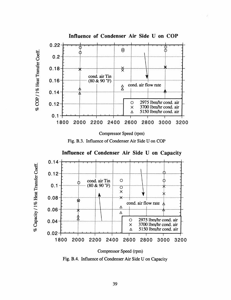
Fig. B.3. Influence of Condenser Air Side U on COP
Influence of Condenser Air Side U on Capacity 0.14 I I ~ ~ I I
o 1 2 - ...................... 1.. .................... 1. .................... .1 ...................... 1. ............ \ ....... L ................... ~ .................... -. I con1 air Tin I 0 I I ~ <D ::::
o ~~: ~=r=~:r:·:-G:I;l=I:~=:: i I I c~nd. air fl~w rate l
::::~:=~~t=--f-~=P--~iste;~~i~ 0.02 I I I I I I
1800 2000 2200 2400 2600 2800 3000 3200
Compressor Speed (rpm)
Fig. B.4. Influence of Condenser Air Side U on Capacity
39

Influence of Condenser Refrigerant Side U on COP
0.34-~~4~~~-~i'~~~1~~~'~~~'~~-~'~~
i condo air Tin i
::::~ ~jJ~·:t~t.,tj~ * I I ~ I I ~ 0024--Hi--rmr rnre t-
0.22 - ······················,····················t···················t··········· ~ ~~~ ~~= ~~~~:: ~ iii f). 5150 Ibm/hr condo air
0.2;-~~~;~~-r,:~~~;~~~,-----~,----~,----r
1800 2000 2200 2400 2600 2800 3000 3200
Compressor Speed (rpm)
Fig. B.5. Influence of Condenser Refrigerant Side U on COP
Influence of Condenser Refrigerant Side U on Capacity
0.161-~~+'~~_~'~~'~~~'~~_~'~~y~~~
0\* O. 1 4 - .................... ~ ................... + ..................... + ..................... j ............... ······f·····················+····················· ~
i condo air Tin iii cb I (80 ~ 90 oF) I x I I 1
0.12 - ·····················f·················T·~················r······~·········r················fr···················f···················· -
001 --it -/:-t m fltw rnret- ~
Ooos----rrrr ~ ~r~!==~-0.06 I I I I I I
1800 2000 2200 2400 2600 2800 3000 3200
Compressor Speed (rpm)
Fig. B.6. Influence of Condenser Refrigerant Side U on Capacity
40

Influence of Condenser Pressure Drop on COP
-0.00054-~~~~~~_~I~~i~~~'~~~'~~_~I~~
.... -0 .001 - ····················~····················t······················I········g·········j·················· ····I·····················qL ................. '""" B iii Xii * ~ -0 .001 5 - ..................... * ......... cond air Tin 1······················j·················· ... ~ .................... ~ .................... -~ i (80 & 90 OF) i 0 iii c:: : : A: : A .g -0 . 002 - ····················-Q····················t············ .......... [......... ·········1················~ , ... [ ..................... * .................... r-.g ~ i ,~ i X l l i
~~~~:~~:~==-E=t=Ej~3~=: ~ 1 1 1 0 2975 Ibm/hr condo air
-0 .004 - ····················i···················+············· ...... +........... x 3700 Ibm/hr condo air r-i 1 1 f::. 5150 Ibm/hr condo air
-0.0045 ; : ; I I I
1800 2000 2200 2400 2600 2800 3000 3200
Compressor Speed (rpm)
Fig. B.7. Influence of Condenser Pressure Drop on COP
Influence of Condenser Pressure Drop on Capacity
-0.0002;-~~~1~~_~1~~1~~~1----~1----_~1--~ o 29751bm/hrcond.air
~ -0.0003 - ······················1······················+······················1············ x 3700 Ibm/hr condo ~ r-~ i l i f::. 5150 Ibm/hr condo alf ~ . d' T' . 5 -0.0004 - .................... ·9 ...... · (~3 & ~ 0:.) ·1 ........ ·0 ........ 1 .................... ·+ .................... + .................... ·-
!~:: :::: ~ :=·~;=i1-=t~-;ftj~=t:~:: '0 ~ 1 1 ~ 1 1 A I:ts - 0 . 0007 - .................. · .. ·1 ................ · .. · .. + ................... + ..................... ~ ....... : .............. f ..................... 'f .................... r-fJ< 1 1 1 condo alf flow rate 1
~ -0 .0008 - .................. · .. ·1 .................... ·+ .................... ·1 .................... ·+ ................... + .................... 1-................... r-! i ! ! ! !
-0.0009;-~~+:~~-r,:~~~;~~~;~~-~,:~~-,~: ~~~
1800 2000 2200 2400 2600 2800 3000 3200
Compressor Speed (rpm)
Fig. B.8. Influence of Condenser Pressure Drop on Capacity
41

Influence of Compressor Volume on COP
-0.484-~-r~'-r~~'~~~'~~_~'-r~~'-r~~'~~ . ~
-0 . 5 - .. ······ .... ··········/ ...................... j····· .. ··········· .... ·I .. ·······~· ...... ··j.· .... · ................ 1 ........ ····· ........ 6 .. ···· ............ ·· r-6 condo air !in l l l
- 0 . 52 - .................... ·f .. · .... · (80 i& 90 F) i ...................... 1" ..................... , ...................... 1" .................... -
: :,: : : ~ -0 . 54 - .................... ·t .................... ·j .. · .................. f ...................... j .................... · .. f ...................... t .................... r-; ; ; 0; ; ;
-0 . 5 6 --I-Ij-~!j-·+ ~ _ 0 58 - ...................... ; ...................... j ...................... ·i............ 0 2975 lbm/hr condo air -
. 0:: X 3700lbm/hrcond.air ± I I D. 5150 lbm/hr condo air -0.6~~~~,~~~,~~~,~~-~,----r-,----~,----r
1800 2000 2200 2400 2600 2800 3000 3200
Compressor Speed (rpm)
Fig. B.9. Influence of Compressor Volume on COP
Influence of Compressor Volume on Capacity
0.34
t ~ 0.3 ='
-0 > 0.26 ~ -' -C-.... 0.22 ~ §' U ~ 0.18
0.14
..................... ~ ..................... ~ ................... ) ...................... i ....................... 1 ...................... i .................... .. x : : D.' . : ! j j D. condo air flow rate j 8: ; ; ! ! ; . : : x: : :
...................... 1 ...................... ( .................. ·( .. · .............. ·: .............. · ...... ! ..................... ~ .................... . : : : x: : X l j l <:5 i l *
...................... 1.... condo air Tin ..... j .................... ) .................... ) .................... ..j ..................... .
I (80 & 90 OF) I I I $
-Ill ~ ~I~ leE :s: ~ 1800 2000 2200 2400 2600 2800 3000 3200
Compressor Speed (rpm)
Fig. B.I0. Influence of Compressor Volume on Capacity
42
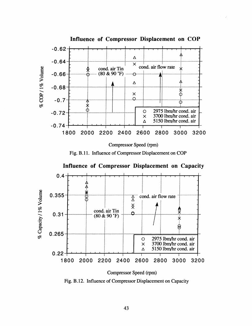
Influence of Compressor Displacement on COP
-0.621-~~~'~~~'-r~~'~~~'~~_~'-r~~'-r~~ :::! i ; t
-0 . 64 - ···· .. ········ .. ······j···················· .. t· .. ··········· .. ·····+········~···· .. ···I······················+···· ................ + ..................... -~ condo air Tin . co~d. air fl~w rate *
o 2975 lbm/hr condo air ex 37oolbm/hrcond.air
j j j l!1 5150 lbm/hr condo air -0.741-~~~I~~~,~~~,~~-~,----r-,----~,----r
1800 2000 2200 2400 2600 2800 3000 3200
Compressor Speed (rpm)
Fig. B.1l. Influence of Compressor Displacement on COP
Influence of Compressor Displacement on Capacity
0.44-~~~'~~~'~~~'~~_~'~~~'~~~'~~~
!
* o . 355 - ····················i····················t······················I·········~···· c~nd. air fl~w rate .. j ...................... r-
0.31 ---I <:i ~:~ J~l-!.~J- ~ 1 : 1 1 1 ),<
I I I I I ~ 0.265- ········ ...... · ...... ·j .. · ...... · ........ · .. ·t .. · .......... ·· ...... ·1 ...... · .. · ............ i ...................... .: ...................... i ..................... .
! ! ! 0 2975 lbm/hr condo air ! ! ! x 3700 lbm/hr condo air I I I l!1 5150 lbm/hr condo air
0.221-~~~,~~~,~~~,~~~,-----r-,----r-,----r
1800 2000 2200 2400 2600 2800 3000 3200
Compressor Speed (rpm)
Fig. B.12. Influence of Compressor Displacement on Capacity
43

Influence of Evaporator Air Side U on COP
0.08~~~~'~~_~'~~'~~~'----~'----_~'----r i l ' 0 2975 lbm/hr condo air
o .07 - ······················1····················+·····················1············ x 3700 lbm/hr condo air -~ i i ~ 5150Ibm/hrcond.air
o .06 - ······················1·· .. condo !rr flow ~te ··ts·······t·····················(···················l ...................... r-
0.05 - ····················t··················+····~········· ... + ........ ~ ......... j ................. ····1·····················1-··················· r-
:·::~:=~t=t:--~j~::t:t=t=~~ ~ . !! I 0 Icond.~Tin I
o . 02 - ·····················r···················r···················r···················"/" (80 & 90 OF) ........ ~ .................... r-! i ! i ! 0.01~~~~1~~-~1~~1~~~1~~~~1~~1~~~
1800 2000 2200 2400 2600 2800 3000 3200
Compressor Speed (rpm)
Fig. B.13. Influence of Evaporator Air Side U on COP
Influence of Evaporator Air Side U on Capacity
O 155 I 1 I I I I . 1---0--.29-7-5-lb-m/hr~-c-o-nd-.• arr-.~~~~~~~~~~i ~-r~
X 3700lbm/hrcond.air l 0.15 - ~ 5150 lbm/hr condo air ~·········J·······················i··················· ... j ...................... -
ii'
O. 1 45 - ·····················J····················t··· ·················f·········~·········j··· condo ~ Tin ....... j ...................... r-i ! ~ ! x ! (80 & 90 OF) ~
001·::~=h[:~:t::II=t~~~ I I I I I f 0.13;-~~+,~~-~,~~,~~~,~~-~,~~,~~~
1800 2000 2200 2400 2600 2800 3000 3200
Compressor Speed (rpm)
Fig. B.14. Influence of Evaporator Air Side U on Capacity
44

Influence of Evaporator Refrigerant Side U on COP 0.018 I I I I I I
0.016 - ················· .... t.··· ..... ····· ... ····t······················1············ ~ ~~~ ~~= ~~~~:: ~ 1 1 1 ~ 51501b~cond.arr 0.014- ······················i······················i-········ .............. ! ......... ~ ....... : ............................................................ .
! condo ~ flow ~te ! ! ! o . 0 1 2 - .................... )ir .................... , ...................... , ..................... .,. .................... , ...................... , ...................... -~ 1 ~ 1 ~ 1 1 t o .01 - ·····················+·····················t····· ···············I······················j··············· ... ····t······················!······················ -
~ i i xii ~
~:~~:~~=+=1= =T:~.r~~f=::=: iii i condo arrTm cb
0.004- ······················1······················t······················[······················1· (80 & 90 OF) ......... ( ................... -
0.0024-~~+!~~_~I1~~~!~~~!~~-~I~~~~~~ 1800 2000 2200 2400 2600 2800 3000 3200
Compressor Speed (rpm)
Fig. B.15. Influence of Evaporator Refrigerant Side U on COP
Influence of Evaporator Refrigerant Side U on Capacity
I:ci 0.038
8 0.036 ~ 0.034 c,.;;, fI)
~ F= 0.032 ~
~ 0.03 ~
0.028 --~ 0.026 .... ~ g.
0.024 u ~
0.022
o 29751b~cond.arr .................... A .................... L .................. .L........... x 3700 Ib~ condo arr
, 1 1 ~ 51501b~cond. arr ...................... , ... condo r flow rafe ················r···················· ., .................... 1" .................. . ·····················t·····················t······ ···········I·········~·········j······················I······················j······················
==~B=t __ ~!====£=~~f.:= iii 0 i condo arrTin i ······················j······················t······················1······················)··· (80 & 90 OF) ....... ) ..................... .
! ! ! i <b
1800 2000 2200 2400 2600 2800 3000 3200
Compressor Speed (rpm)
Fig. B.16. Influence of Evaporator Refrigerant Side U on Capacity
45

REFERENCES
Internal Publications
Kempiak, M. Three-Zone Modeling of a Mobile Air Conditioning Condenser. ACRC TR-03, April, 1991.
Siambekos, C. Two-Zone Modeling of a Mobile Air Conditioning Plate-Fin Evaporator. ACRC TR-05, October, 1991.
Darr,l. Modeling of an Automotive Air Conditioning Compressor Based on Experimental Data. ACRC TR-14, March, 1992.
VanderZee, 1. Semi-Theoretical Steady State and Transient Modeling of a Mobile Air Conditioning Condenser. ACRe TR-36, May, 1993.
Smith, S. Semi-Theoretical Steady State and Transient Modeling of an Automotive Air Conditioning Evaporator. ACRC TR-37, May, 1993.
External Reference
Eckels, S.l. and Pate, M.B.1991. Evaporation and Condensation of HFC-134a and CFC-12 in a Smooth Tube and a Micro-Fin Tube. ASHRAE Transactions Vol. 97 Part 2. Atlanta, GA.
46