mixtures 4
DESCRIPTION
estadisticaTRANSCRIPT
7/17/2019 Mixtures 4
http://slidepdf.com/reader/full/mixtures-4 1/11
Finite Mixture Modelling
Model Specification, Estimation & Application
Bettina Grun
Department of Statistics and Mathematics
Research Seminar, November 23 2007
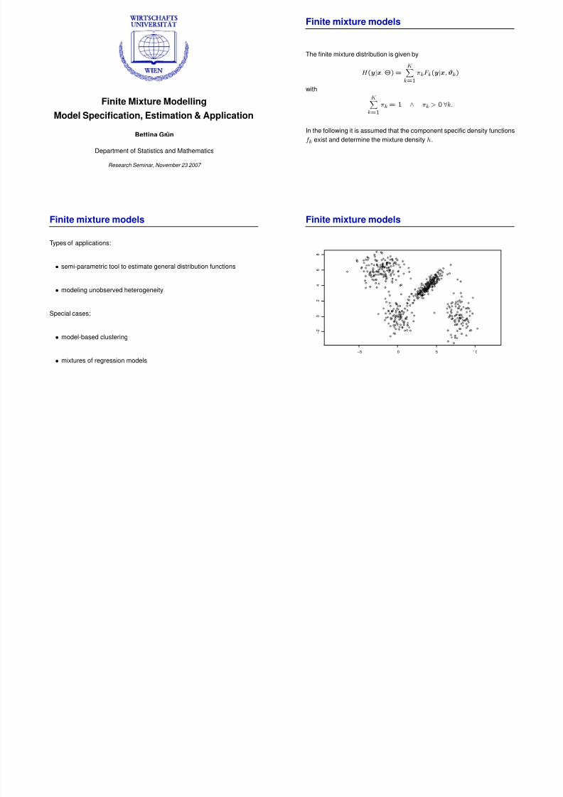
Finite mixture models
The finite mixture distribution is given by
H (y|x, Θ) =K
k=1
πkF k(y|x,ϑk)
with
K
k=1
πk = 1 ∧ πk > 0 ∀k.
In the following it is assumed that the component specific density functions
f k exist and determine the mixture density h.
Finite mixture models
Types of applications:
• semi-parametric tool to estimate general distribution functions
• modeling unobserved heterogeneity
Special cases:
• model-based clustering
• mixtures of regression models
Finite mixture models
−5 0 5 10
− 2
0
2
4
6
8
7/17/2019 Mixtures 4
http://slidepdf.com/reader/full/mixtures-4 2/11
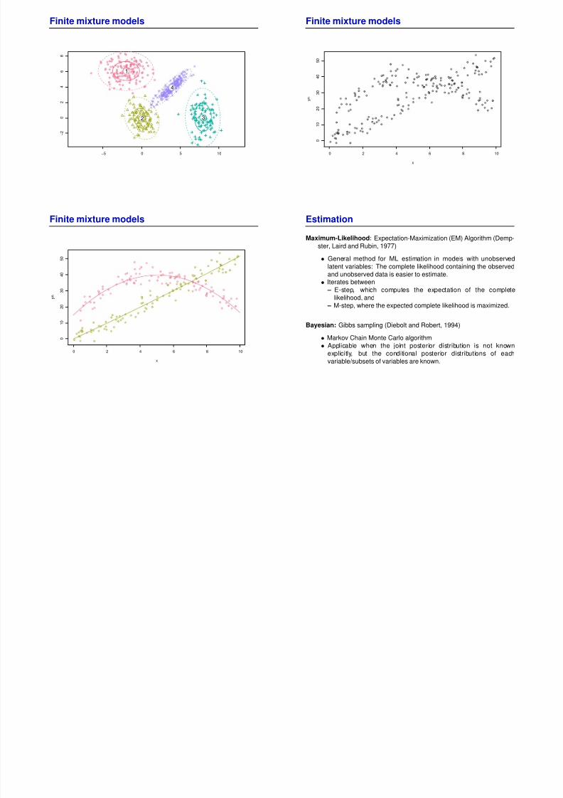
Finite mixture models
−5 0 5 10
− 2
0
2
4
6
8
1
2 3
4
Finite mixture models
0 2 4 6 8 10
0
1 0
2 0
3 0
4 0
5 0
x
y n
Finite mixture models
0 2 4 6 8 10
0
1 0
2 0
3 0
4 0
5 0
x
y n
Estimation
Maximum-Likelihood: Expectation-Maximization (EM) Algorithm (Demp-
ster, Laird and Rubin, 1977)
• General method for ML estimation in models with unobserved
latent variables: The complete likelihood containing the observed
and unobserved data is easier to estimate.• Iterates between
– E-step, which computes the expectation of the complete
likelihood, and
– M-step, where the expected complete likelihood is maximized.
Bayesian: Gibbs sampling (Diebolt and Robert, 1994)
• Markov Chain Monte Carlo algorithm• Applicable when the joint posterior distribution is not known
explicitly, but the conditional posterior distributions of each
variable/subsets of variables are known.

7/17/2019 Mixtures 4
http://slidepdf.com/reader/full/mixtures-4 3/11
Missing data
The component-label vectors zn = (znk)k=1,...,K are treated as missing
data. It holds that
• znk ∈ {0, 1} and
• K
k=1 znk = 1 for all k = 1, . . . , K .
The complete log-likelihood is given by
log Lc(Θ) =K
k=1
N
n=1
znk [log πk + log f k(yn|xn,ϑk)] .
EM algorithm: E-step
Given the current parameter estimates Θ(i) replace the missing data z nk
by the estimated a-posteriori probabilities
z(i)nk = P(k|yn,xn,Θ(i)) =
π(i)k
f k(yn|xn,ϑ(i)k )
K
u=1
π(i)u f k(yn|xn,ϑ
(i)u )
.
The conditional expectation of log Lc(Θ) at the ith step is given by
Q(Θ;Θ(i)) = EΘ(i) [log Lc(Θ)|y,x]
=K
k=1
N
n=1
z(i)nk [ log πk + log f k(yn|xn,ϑk)] .
EM algorithm: M-step
The next parameter estimate is given by:
Θ(i+1) = argmaxΘ
Q(Θ;Θ(i)).
The estimates for the prior class probabilities are given by:
π(i+1)k = 1
N
N
n=1
z(i)nk
.
The component specific parameter estimates are determined by:
ϑ(i+1)k = argmax
ϑk
N
n=1
z(i)nk log(f k(yn|xn,ϑk)).
⇒ weighted ML estimation of the component specific model.
M-step: Mixtures of Gaussian distributions
The solutions for the M-step are given in closed form:
µ(i+1)k =
N n=1 z
(i)nkyn
N n=1 z
(i)nk
Σ(i+1)k =
N n=1 z
(i)nk (yn − µ
(i+1)k )(yn − µ
(i+1)k )
N n=1 z
(i)nk
7/17/2019 Mixtures 4
http://slidepdf.com/reader/full/mixtures-4 4/11
Estimation: EM algorithm
Advantages:
• The likelihood is increased in each step → EM algorithm converges
for bounded likelihoods.
• Relatively easy to implement:
– Different mixture models require only different M-steps.
– Weighted ML estimation of the component specific model is
sometimes already available.
Disadvantages:
• Standard errors have to be determined separately as the information
matrix is not required during the algorithm.
• Convergence only to a local optimum
• Slow convergence
⇒ variants such as Stochastic EM (SEM) or Classification EM (CEM)
EM algorithm: Number of components
Information criteria: e.g. AIC, BIC, ICL
Likelihood ratio test statistic: Comparison of nested models where the
smaller model is derived by fixing one parameter at the border of the
parameter space.
⇒ Regularity conditions are not fulfilled.
The asymptotic null distribution is not the usual χ2-distribution with
degrees of freedom equal to the difference beween the number of
parameters under the null and alternative hypotheses.
• distributional results for special cases
• bootstrapping
Bayesian estimation
Determine the posterior density using Bayes’ theorem
p(Θ|Y ,X ) ∝ h(Y |X , Θ) p(Θ),
where p(Θ) is the prior and Y = (yn)n and X = (xn)n.
Standard prior distributions:
• Proper priors: Improper priors give improper posteriors.
• Independent priors for the component weights and the component
specific parameters.
• Conjugate priors for the complete likelihood
– Dirichlet distribution D(e0,1, . . . , e0,K ) for the component weights
which is the conjugate prior for the multinomial distribution.
– Priors on the component specific parameters depend on the
underlying distribution family.
• Invariant priors, e.g. the parameter for the Dirchlet prior is constant
over all components: e 0,k ≡ e0.
Estimation: Gibbs sampling
Starting with Z 0 = (z0n)n=1,...,N repeat the following steps for i =
1, . . . , I 0, . . . , I + I 0.
1. Parameter simulation conditional on the classificationZ (i−1):
(a) Sample π1, . . . , πK from D((N
n=1 z(i−1)nk + e0,k)k=1,...,K ).
(b) Sample component specific parameters from the complete-data
posterior p(ϑ1, . . . , ϑK |Z (i−1)
,Y )Store the actual values of all parameters Θ(i) = (π
(i)k
,ϑ(i)k )k=1,...,K .
2. Classification of each observation (yn,xn) conditional on knowing
Θ(i):
Sample z(i)n from the multinomial distribution with parameter equal to
the posterior probabilities.
After discarding the burn-in draws the draws I 0 + 1, . . . , I + I 0 can be
used to approximate all quantities of interest.

7/17/2019 Mixtures 4
http://slidepdf.com/reader/full/mixtures-4 5/11
Example: Gaussian distribution
Assume an independence prior
p(µk, Σ−1k ) ∼ f N (µk; b0,B0)f W (Σ−1
k ; c0,C 0).
1. Parameter simulation conditional on the classificationZ (i−1):
(a) Sample π(i)1 , . . . , π
(i)K from D((
N n=1 z
(i−1)nk + e0,k)k=1,...,K ).
(b) Sample (Σ−1k )(i) i n e ac h grou p k f ro m a Wis ha rt
W (ck(Z (i−1)),C k(Z (i−1))) distribution.(c) Sample µ
(i)k in each group k from a N (bk(Z (i−1)),Bk(Z (i−1)))
distribution.
2. Classification of each observation yn conditional on knowing Θ(i):
P(z(i)nk = 1|yn, Θ(i)) ∝ πkf N (yn;µk, Σk)
Estimation: Gibbs sampling
Advantages:
• Relatively easy to implement
– Different mixture models differ only in the parameter simulation
step.
– Parameter simulation conditional on the classification is sometimes
already available.
Disadvantages:
• Might fail to escape the attraction area of one mode → not all posterior
modes are visited.
Gibbs sampling: Number of components
• Bayes factors
• Sampling schemes with a varying number of components
– reversible-jump MCMC
– inclusion of birth-and-death processes
Label switching
The posterior distribution is invariant under a permutation of the
components with the same component-specific model.
⇒ Determine a unique labelling for component-specific inference:
• Impose a suitable ordering constraint, e.g. πs < πt ∀s, t ∈ {1, . . . , S }
with s < t.
• Minimize the distance to the Maximum-A-Posteriori (MAP) estimate.
• Fix the component membership for some observations.
• Relabelling algorithms.

7/17/2019 Mixtures 4
http://slidepdf.com/reader/full/mixtures-4 6/11
Initialization
• Construct a suitable parameter vector Θ(0).
– random
– other estimation methods: e.g. moment estimators
• Classify observations/assign a-posteriori probabilities to each obser-
vation.
– random
– cluster analysis results: e.g. hierarchical clustering, k-means
Extensions and special cases
• Model-based clustering:
– Latent class analysis: multivariate discrete observations where the
marginal distributions in the components are independent.
– mixtures of factor analyzers
– mixtures of t-distributions
• Mixtures of regressions:
– mixtures of generalized linear models
– mixtures of generalized linear mixed models
• Covariates for the component sizes: concomitant variable models
• Impose equality constraints between component-specific parameters
Software in R
• Model-based clustering:
– mclust (Fraley and Raftery, 2002) for Gaussian mixtures:
∗ specify different models depending on the structure of the
variance-covariance matrices (volume, shape, orientation)
Σk = λkDkdiag(ak)Dk
∗ initialize EM algorithm with the solution from an agglomerativehierarchical clustering algorithm
• Clusterwise regression:
– flexmix (Leisch, 2004)
See also CRAN Task View “Cluster Analysis & Finite Mixture Models”.
Software: FlexMix
• The function flexmix() provides the E-step and all data handling.
• The M-step is supplied by the user similar to glm() families.
• Multiple independent responses from different families
• Currently bindings to several GLM families exist (Gaussian, Poisson,
Gamma, Binomial)• Weighted, hard (CEM) and random (SEM) classification
• Components with prior probability below a user-specified threshold are
automatically removed during iteration
7/17/2019 Mixtures 4
http://slidepdf.com/reader/full/mixtures-4 7/11
FlexMix Design
• Primary goal is extensibility: ideal for trying out new mixture models.
• No replacement of specialized mixtures like mclust(), but comple-
ment.
• Usage of S4 classes and methods
• Formula-based interface
• Multivariate responses:combination of univariate families: assumption of independence
(given x), each response may have its own model formula, i.e.,
a different set of regressors
multivariate families: if family handles multivariate response directly,
then arbitrary multivariate response distributions are possible
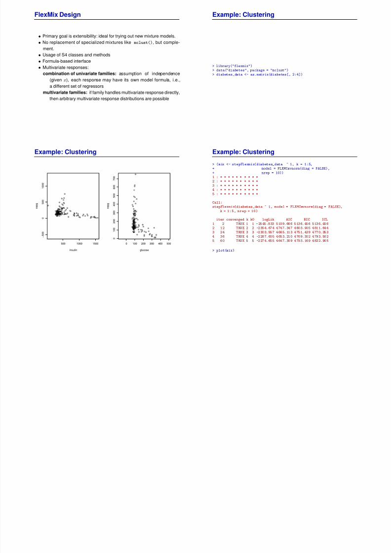
Example: Clustering
> library("flexmix")> data("diabetes", package = "mclust")> diabetes_data <- as.matrix(diabetes[, 2:4])
Example: Clustering
500 1000 1500
− 5 0 0
0
5 0 0
1 0 0 0
insulin
s s p g
0 100 200 300 400 500
0
1 0 0
2 0 0
3 0 0
4 0 0
5 0 0
6 0 0
7 0 0
glucose
s s p g
Example: Clustering
> (mix <- stepFlexmix(diabetes_data ~ 1, k = 1:5,+ model = FLXMCmvnorm(diag = FALSE),+ nrep = 10))1 : * * * * * * * * * *2 : * * * * * * * * * *3 : * * * * * * * * * *4 : * * * * * * * * * *5 : * * * * * * * * * *
Call:stepFlexmix(diabetes_data ~ 1, model = FLXMCmvnorm(diag = FALSE),
k = 1:5, nrep = 10)
iter converged k k0 logLik AIC BIC ICL1 2 TRUE 1 1 -2545.833 5109.666 5136.456 5136.4562 12 TRUE 2 2 -2354.674 4747.347 4803.905 4811.6443 24 TRUE 3 3 -2303.557 4665.113 4751.439 4770.3534 36 TRUE 4 4 -2287.605 4653.210 4769.302 4793.5025 60 TRUE 5 5 -2274.655 4647.309 4793.169 4822.905
> plot(mix)

7/17/2019 Mixtures 4
http://slidepdf.com/reader/full/mixtures-4 8/11
Example: Clustering
1 2 3 4 5
4 7 0 0
4 8 0 0
4 9
0 0
5 0 0 0
5 1 0 0
number of components
AICBICICL
Example: Clustering
> (mix_best <- getModel(mix))Call:stepFlexmix(diabetes_data ~ 1, model = FLXMCmvnorm(diag = FALSE),
k = 3, nrep = 10)
Cluster sizes:1 2 3
82 28 35
convergence after 24 iterations
> summary(mix_best)Call:stepFlexmix(diabetes_data ~ 1, model = FLXMCmvnorm(diag = FALSE),
k = 3, nrep = 10)
prior size post>0 ratioComp.1 0.540 82 101 0.812C omp .2 0 .1 99 2 8 9 6 0 .2 92Comp.3 0.261 35 123 0.285
’log Lik.’ -2303.557 (df=29)AIC: 4665.113 BIC: 4751.439
Example: Clustering
500 1000 1500
− 5 0 0
0
5 0 0
1 0 0 0
insulin
s s p g
12
3
0 100 200 300 400 500
0
1 0 0
2 0 0
3 0 0
4 0 0
5 0 0
6 0 0
7 0 0
glucose
s s p g
1
2
3
Example: Clustering
> table(cluster(getModel(mix)), diabetes$class)chemical normal overt
1 10 72 02 1 0 273 25 4 6
> parameters(mix_best, component = 1, simplify = FALSE)$center
glucose insulin sspg91.00937 358.19098 164.14443
$covg luc os e in su li n s sp g
glucose 58.21456 80.1404 16.8295insulin 80.14039 2154.9810 347.6972sspg 16.82950 347.6972 2484.1538> plot(mix_best, mark = 2)
7/17/2019 Mixtures 4
http://slidepdf.com/reader/full/mixtures-4 9/11
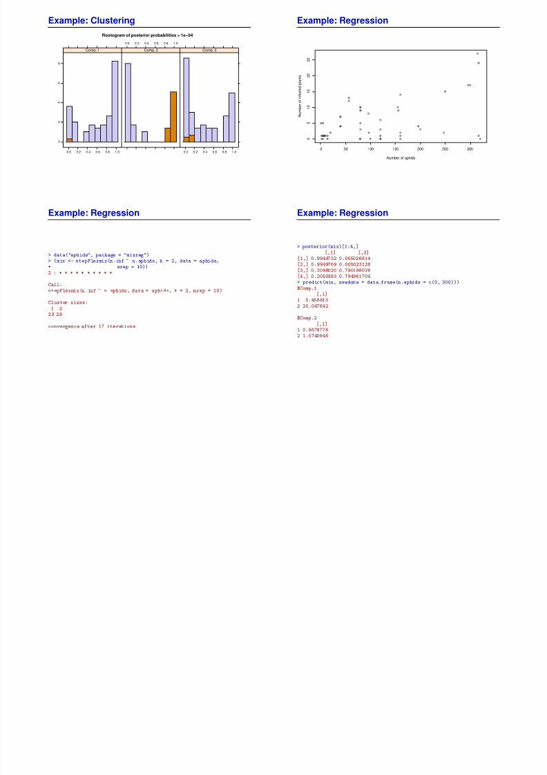
Example: Clustering
Rootogram of posterior probabilities > 1e−04
0
2
4
6
8
0 .0 0 .2 0 .4 0 .6 0 .8 1 .0
Comp. 1
0 .0 0 .2 0 .4 0 .6 0 .8 1 .0
Comp. 2
0 .0 0 .2 0 .4 0 .6 0 .8 1 .0
Comp. 3
Example: Regression
0 50 100 150 200 250 300
0
5
1 0
1 5
2 0
2 5
Number of aphids
N u m b e r o f i n f e c t e d p l a n t s
Example: Regression
> data("aphids", package = "mixreg")> (mix <- stepFlexmix(n.inf ~ n.aphids, k = 2, data = aphids,+ nrep = 10))2 : * * * * * * * * * *
Call:stepFlexmix(n.inf ~ n.aphids, data = aphids, k = 2, nrep = 10)
Cluster sizes:1 2
23 28
convergence after 17 iterations
Example: Regression
> posterior(mix)[1:4,][,1] [,2]
[1,] 0.9949732 0.005026814[2,] 0.9949769 0.005023128[3,] 0.2098020 0.790198026[4,] 0.2050383 0.794961704> predict(mix, newdata = data.frame(n.aphids = c(0, 300)))
$Comp.1[,1]
1 3.4588132 20.047842
$Comp.2[,1]
1 0.86797762 1.5740946
7/17/2019 Mixtures 4
http://slidepdf.com/reader/full/mixtures-4 10/11
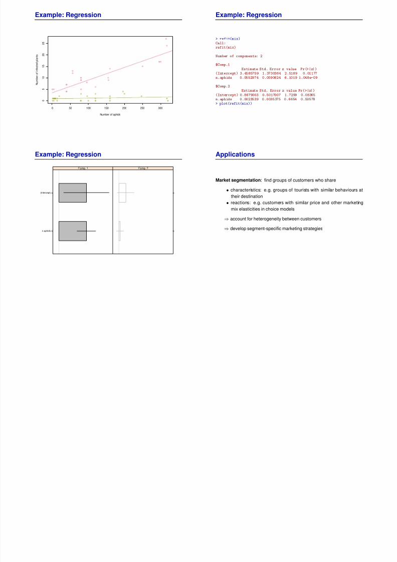
Example: Regression
0 50 100 150 200 250 300
0
5
1 0
1 5
2 0
2 5
Number of aphids
N u m b e r o f i n f e c t e d p l a n t s
Example: Regression
> refit(mix)Call:refit(mix)
Number of components: 2
$Comp.1
Estimate Std. Error z value Pr(>|z|)(Intercept) 3.4585759 1.3730364 2.5189 0.01177n.aphids 0.0552974 0.0090624 6.1019 1.048e-09
$Comp.2Estimate Std. Error z value Pr(>|z|)
(Intercept) 0.8679003 0.5017007 1.7299 0.08365n.aphids 0.0023539 0.0035375 0.6654 0.50578> plot(refit(mix))
Example: Regression
n.aphids
(Intercept)
Comp. 1 Comp. 2
Applications
Market segmentation: find groups of customers who share
• characteristics: e.g. groups of tourists with similar behaviours at
their destination
• reactions: e.g. customers with similar price and other marketing
mix elasticities in choice models
⇒ account for heterogeneity between customers
⇒ develop segment-specific marketing strategies

7/17/2019 Mixtures 4
http://slidepdf.com/reader/full/mixtures-4 11/11
Monographs
D. Bohning.Computer Assisted Analysis of Mixtures and Applications:
Meta-Analysis, Disease Mapping, and Others . Chapman & Hall/CRC,
London, 1999.
S. Fruhwirth-Schnatter. Finite Mixture and Markov Switching Models .
Springer Series in Statistics. Springer, New York, 2006.
B. G. Lindsay. Mixture Models: Theory, Geometry, and Applications . The
Institute for Mathematical Statistics, Hayward, California, 1995.
G. J. McLachlan and K. E. Basford. Mixture Models: Inference and
Applications to Clustering . Marcel Dekker, New York, 1988.
G. J. McLachlan and D. Peel. Finite Mixture Models . Wiley, 2000.
References
A. P. Dempster, N. M. Laird, and D. B. Rubin. Maximum likelihood from
incomplete data via the EM-algorithm. Journal of the Royal Statistical
Society B , 39:1–38, 1977.
J. Diebolt and C. P. Robert. Estimationof finitemixture distributions through
Bayesian sampling. Journal of the Royal Statistical Society B , 56:363–375,
1994.
C. Fraley and A. E. Raftery. Model-based clustering, discriminant analysis
and density estimation. Journal of the American Statistical Association , 97
(458):611–631, 2002.
F. Leisch. FlexMix: A general framework for finite mixture models and
latent class regression in R. Journal of Statistical Software , 11(8), 2004.
URL http://www.jstatsoft.org/v11/i08/.