mixed methods with weak symmetry for time dependent …arnold/papers/leethesis.pdf · ·...
TRANSCRIPT

Mixed methods with weak symmetry for time dependentproblems of elasticity and viscoelasticity
A DISSERTATION
SUBMITTED TO THE FACULTY OF THE GRADUATE SCHOOL
OF THE UNIVERSITY OF MINNESOTA
BY
Jeonghun Lee
IN PARTIAL FULFILLMENT OF THE REQUIREMENTS
FOR THE DEGREE OF
Doctor of Philosophy
Douglas N. Arnold
July, 2012

c© Jeonghun Lee 2012
ALL RIGHTS RESERVED

Acknowledgements
I would like to express my gratitude to all people who supported me to complete
this thesis. First of all, I am very thankful to all of my family members who
supported my graduate studies for years. I want to show my deepest appreci-
ation to my advisor, Douglas N. Arnold, who always supported me in all the
best ways. I am specially thankful to Prof. Mori Yoichiro for encouraging my
studies and valuable advice. I also have to confess that many of my colleagues
supported my studies who I cannot list all names here. I am grateful for com-
puting resources from the University of Minnesota Supercomputing Institute.
I gratefully acknowledge the support I received during the preparation of this
thesis through National Science Foundation grant DMS-1115291.
i

Abstract
In this dissertation, we study numerical algorithms for time dependent problems
in continuum mechanics using mixed finite element methods. We are particu-
larly interested in linear elastodynamics and the Kelvin–Voigt, Maxwell, and
generalized Zener models in linear viscoelasticity. We use mixed finite elements
for elasticity with weak symmetry of stress, and show the a priori error analysis.
A main contribution of our analysis is proving existence of a new elliptic projec-
tion map, called a weakly symmetric elliptic projection. In our analysis we prove
that a priori error estimates for elastodynamics and viscoelasticity problems are
as good as that of stationary elasticity problems. We present numerical results
supporting our error analysis. We also present some basic numerical simulations
which are more involved in physical situations.
ii

Contents
Acknowledgements i
Abstract ii
List of tables vi
List of figures vii
1 Introduction 1
1.1 Motivations . . . . . . . . . . . . . . . . . . . . . . . . . . . . . . 1
1.2 Mixed finite element methods for elasticity . . . . . . . . . . . . 3
1.3 Mixed methods for time dependent elasticity and viscoelasticity . 9
1.4 Overview of chapters . . . . . . . . . . . . . . . . . . . . . . . . . 11
2 Preliminaries 14
2.1 Notations and definitions . . . . . . . . . . . . . . . . . . . . . . 14
2.2 Continuum mechanics . . . . . . . . . . . . . . . . . . . . . . . . 17
2.2.1 Deformation, strain, momenta, and stress . . . . . . . . . 17
2.2.2 Linear elasticity . . . . . . . . . . . . . . . . . . . . . . . 20
2.2.3 Linear viscoelasticity . . . . . . . . . . . . . . . . . . . . . 21
2.3 Mixed finite element methods . . . . . . . . . . . . . . . . . . . . 25
2.3.1 Saddle point problems . . . . . . . . . . . . . . . . . . . . 25
2.3.2 Mixed finite elements and Brezzi conditions . . . . . . . . 27
2.4 Mixed finite elements for linear elasticity with weak symmetry . 28
2.4.1 Mixed formulations of linear elasticity . . . . . . . . . . . 29
2.4.2 Two families of stable mixed finite elements for elasticity 31
2.4.3 Error analysis for linear elasticity . . . . . . . . . . . . . . 34
2.4.4 A weakly symmetric elliptic projection . . . . . . . . . . . 42
2.5 Miscellaneous preliminaries . . . . . . . . . . . . . . . . . . . . . 43
iii

2.5.1 Gronwall-type estimates . . . . . . . . . . . . . . . . . . . 43
2.5.2 Well-posedness of differential algebraic equations . . . . . 45
2.5.3 Regularity lemmas . . . . . . . . . . . . . . . . . . . . . . 46
3 Mixed methods for linear elastodynamics 49
3.1 Introduction . . . . . . . . . . . . . . . . . . . . . . . . . . . . . . 49
3.2 Weak formulations with weak symmetry . . . . . . . . . . . . . . 50
3.3 Semidiscrete problems . . . . . . . . . . . . . . . . . . . . . . . . 54
3.3.1 Existence and uniqueness of semidiscrete solutions . . . . 55
3.3.2 Decomposition of semidiscrete errors . . . . . . . . . . . . 56
3.3.3 Projection error estimates for the AFW elements . . . . . 57
3.3.4 Approximation error estimates for the AFW elements . . 58
3.4 Full discretization . . . . . . . . . . . . . . . . . . . . . . . . . . . 60
3.4.1 Well-definedness . . . . . . . . . . . . . . . . . . . . . . . 61
3.4.2 Convergence . . . . . . . . . . . . . . . . . . . . . . . . . 62
3.5 Error analysis for the GG elements . . . . . . . . . . . . . . . . . 67
3.5.1 A priori error estimates . . . . . . . . . . . . . . . . . . . 67
3.5.2 Postprocessing . . . . . . . . . . . . . . . . . . . . . . . . 70
3.6 Robustness for nearly incompressible materials . . . . . . . . . . 72
3.7 Numerical results . . . . . . . . . . . . . . . . . . . . . . . . . . . 76
4 Mixed methods for the Kelvin–Voigt model of viscoelasticity 81
4.1 Introduction . . . . . . . . . . . . . . . . . . . . . . . . . . . . . . 81
4.2 Weak formulations with weak symmetry . . . . . . . . . . . . . . 82
4.3 Semidiscrete problems . . . . . . . . . . . . . . . . . . . . . . . . 86
4.3.1 Existence and uniqueness of semidiscrete solutions . . . . 86
4.3.2 Decomposition of semidiscrete errors . . . . . . . . . . . . 87
4.3.3 Projection error estimates for the AFW elements . . . . . 89
4.3.4 Approximation error estimates for the AFW elements . . 90
4.4 Full discretization . . . . . . . . . . . . . . . . . . . . . . . . . . . 93
4.4.1 Well-definedness . . . . . . . . . . . . . . . . . . . . . . . 94
4.4.2 Convergence . . . . . . . . . . . . . . . . . . . . . . . . . 95
4.5 Error analysis for the GG elements . . . . . . . . . . . . . . . . . 101
4.6 Numerical results . . . . . . . . . . . . . . . . . . . . . . . . . . . 104
5 Mixed methods for the Maxwell and generalized Zener models107
5.1 Introduction . . . . . . . . . . . . . . . . . . . . . . . . . . . . . . 107
iv

5.2 Weak formulations with weak symmetry . . . . . . . . . . . . . . 108
5.3 Semidiscrete problems . . . . . . . . . . . . . . . . . . . . . . . . 112
5.3.1 Existence and uniqueness of semidiscrete solutions . . . . 112
5.3.2 Decomposition of semidiscrete errors . . . . . . . . . . . . 113
5.3.3 Projection error estimates for the AFW elements . . . . . 114
5.3.4 Approximation error estimates for the AFW elements . . 114
5.4 Full discretization . . . . . . . . . . . . . . . . . . . . . . . . . . . 116
5.4.1 Well-definedness . . . . . . . . . . . . . . . . . . . . . . . 117
5.4.2 Convergence . . . . . . . . . . . . . . . . . . . . . . . . . 118
5.5 Error analysis for the GG elements . . . . . . . . . . . . . . . . . 122
5.6 Numerical results . . . . . . . . . . . . . . . . . . . . . . . . . . . 125
6 Numerical simulations 128
6.1 Elastodynamics . . . . . . . . . . . . . . . . . . . . . . . . . . . . 128
6.1.1 Wave propagation in homogeneous isotropic elastic media 128
6.1.2 Wave propagation in isotropic heterogeneous elastic media 129
6.1.3 Wave propagation in anisotropic media . . . . . . . . . . 130
6.2 Viscoelasticity of materials . . . . . . . . . . . . . . . . . . . . . 134
6.2.1 Creep compliance . . . . . . . . . . . . . . . . . . . . . . . 134
6.2.2 Attenuation of reflected waves . . . . . . . . . . . . . . . 135
Bibliography 142
v
List of Tables
1.1 Mixed finite elements for elasticity with triangular meshes . . . . 7
1.2 Mixed finite elements for elasticity with rectangular meshes . . . 8
1.3 Previous studies of mixed methods for elastodynamics . . . . . . 10
1.4 Previous studies of mixed methods for viscoelasticity . . . . . . . 11
3.1 Numerical result 1 of elastodynamics . . . . . . . . . . . . . . . . 77
3.2 Numerical result 2 of elastodynamics . . . . . . . . . . . . . . . . 78
3.3 Numerical result 3 of elastodynamics . . . . . . . . . . . . . . . . 78
3.4 The Butcher’s table for general Runge–Kutta schemes . . . . . . 79
3.5 The Butcher’s table for the 2-stage RadauIIA scheme . . . . . . 79
3.6 Numerical result 4 of elastodynamics . . . . . . . . . . . . . . . . 79
4.1 Numerical result 1 of the Kelvin–Voigt model . . . . . . . . . . . 105
4.2 Numerical result 2 of the Kelvin–Voigt model . . . . . . . . . . . 106
4.3 Numerical result 3 of the Kelvin–Voigt model . . . . . . . . . . . 106
5.1 Numerical result 1 of the Zener model . . . . . . . . . . . . . . . 125
5.2 Numerical result 2 of the Zener model . . . . . . . . . . . . . . . 126
5.3 Numerical result 3 of the Zener model . . . . . . . . . . . . . . . 126
vi
List of Figures
1.1 The lowest order Arnold–Winther elements . . . . . . . . . . . . 5
1.2 The lowest order Arnold–Falk–Winther elements . . . . . . . . . 5
2.1 Mechanical models of viscoelasticity . . . . . . . . . . . . . . . . 24
6.1 Elastic waves in homogeneous isotropic medium . . . . . . . . . . 129
6.2 Elastic wave in heterogeneous isotropic medium 1 . . . . . . . . . 131
6.3 Elastic wave in heterogeneous isotropic medium 2 . . . . . . . . . 132
6.4 Wave propagation in isotropic medium . . . . . . . . . . . . . . . 133
6.5 Wave propagation in orthotropic medium 1 . . . . . . . . . . . . 133
6.6 Wave propagation in orthotropic medium 2 . . . . . . . . . . . . 133
6.7 Creep tests of viscoelastic materials . . . . . . . . . . . . . . . . . 135
6.8 Regions of elastic and viscoelastic materials . . . . . . . . . . . . 135
6.9 Attenuation of reflected wave . . . . . . . . . . . . . . . . . . . . 136
vii

Chapter 1
Introduction
1.1 Motivations
In this dissertation, we study numerical algorithms for linear elastodynamics
and linear viscoelasticity using mixed finite elements for elasticity with weak
symmetry.
Elastic and viscoelastic materials are of great interest in science and engi-
neering because they are involved in many important problems in those areas
with many applications. An elastic material is one of the most fundamental
models of solids in engineering and physics. From the modeling point of view,
an elastic material is regarded as a continuum consisting of infinitesimal springs.
This is a straightforward way to extend a mechanical model to its continuum
version, but it gives a good approximation for the behaviors of many solids when
the deformation of the solids is within a certain small range. Therefore this elas-
tic solid model is very useful for many important problems in solid mechanics
and they have been used for a variety of practical applications. For example, to
design a bridge, we need a good mathematical model for the bridge reflecting
its kinematic features accurately. There are many other important areas that
elastic materials are related, such as seismology in geophysics, so the study of
elastic materials has been and is of great interest. A material is called viscoelas-
tic when it shows kinematic features of both solids and fluids, often called elastic
and viscous behaviors. Purely elastic or purely viscous behaviors of materials
happen only for ideal solids or ideal fluids, respectively. In real life, all solids and
fluids are not ideal, so they have viscoelastic features to some extent. Depend-
1

ing on the manner that the features of solids and fluids are combined, there are
numerous different viscoelastic materials. In many important areas of engineer-
ing, the study of viscoelastic features of materials plays an important role. For
example, most biological tissues show strong viscoelastic features mechanically,
so if we want to develop an artificial organ to replace a tissue, we first have to
understand the viscoelastic features of the tissue very well. Polymeric materials
in rheology are also good examples of viscoelastic materials which have many
important applications.
To study kinematic behaviors of a material theoretically, we express the be-
haviors of the material in mathematical forms. The kinematic behaviors of
elastic and viscoelastic materials are formulated mathematically as partial dif-
ferential equations (PDEs). However, a partial differential equation in material
science is complicated in general even in simple physical models. Not surpris-
ingly, solving the PDE analytically is very difficult, impossible in most cases.
To find solutions of the PDE for practical purposes, we often need a numeri-
cal algorithm to find approximations of the solution with acceptable ranges of
errors.
The numerical study of PDEs is one of the essential tools of modern science
and for practical applications in engineering. For example, through a massive
amount of numerical experiments people observe new phenomena which lead to
improved models of weather prediction. Numerical analysis is also widely used
in designing aircrafts, buildings, and electronic products. As scientists and engi-
neers want to handle more complicated problems which require a large amount
of computations, there is always a great need for faster and more accurate nu-
merical algorithms.
During the last several decades, there have been many important advances in
numerical analysis of PDEs. From the mathematical point of view, various new
and improved numerical algorithms have been developed. The finite element
method is among the most important approaches in the numerical study of
solutions of PDEs. In this dissertation, we study numerical algorithms for time
dependent problems of linear elastic and linear viscoelastic solids using mixed
finite element methods. In our studies, we propose numerical algorithms and
prove that the errors of our numerical solutions have the proposed error bounds.
2

1.2 Mixed finite element methods for elasticity
In this thesis we study mixed methods for time dependent problems of elasticity
and viscoelasticity. Of course, these are based on existing mixed finite elements
for stationary elasticity. Thus, we survey the development of mixed finite ele-
ment methods for elasticity in this section. We will discuss them in more detail
in chapter 2.
In the classical energy minimization form of linear elasticity problems, dis-
placement is the only unknown of the equation and the numerical solution for
stress is obtained using the numerical solution for displacement. In mixed
methods for linear elasticity based on stress and displacement, there are two
unknowns, stress and displacement. At first glance, this approach increases the
number of unknowns and leads to a larger system of equations, but there are
other benefits that make mixed methods attractive. A key advantage of mixed
methods for linear elasticity is that they directly deliver the numerical solution
for stress. Since stress is directly linked to destruction of materials, it is of great
interest in engineering applications. Another advantage of mixed methods for
elasticity is the robustness for nearly incompressible materials. In the displace-
ment based approach, although the error for stress converges to zero as mesh
size converges to zero, the error bound often contains a constant which is very
large when a material is nearly incompressible, so we need a very small mesh
size to get a sufficiently small error. However, the mixed methods we consider
give uniform error bounds for nearly incompressible materials.
Since there are two unknowns, we need a pair of finite element spaces for
mixed methods. One subtlety in mixed methods is to find a pair of finite ele-
ments which guarantee existence of numerical solutions with good approxima-
tion properties. A choice of mixed finite element spaces is called stable if it
guarantees existence of numerical solutions. Necessary and sufficient conditions
for stable mixed finite elements are known based on the foundational work of
Babuska and Brezzi. However, finding stable mixed finite elements for elasticity
has long been a difficult problem. A major obstacle to finding stable mixed fi-
nite elements for elasticity is the symmetry of stress. Since stress is symmetric,
it is natural that the finite elements for stress are symmetric as well, but it is
very difficult to find such stable mixed finite elements for elasticity.
The first mixed finite elements for elasticity were developed by Johnson and
Mercier using composite triangles [36]. For a triangle, three subtriangles are
obtained by connecting an interior point to the three vertices. In the Johnson–
3
Mercier elements, shape functions for stress are the piecewise linear polyno-
mials adapted to the subtriangles satisfying normal continuity on the interior
edges of subtriangles. Because of the construction using composite triangles, it
is complicated to implement these elements. Moreover, generalizations of the
Johnson–Mercier elements to higher order elements or to three dimensions are
not obvious. In two dimensions, there is a family of higher order mixed finite
elements for elasticity developed by Arnold, Douglas, and Gupta using compos-
ite triangles in [8]. They followed an analysis similar to that of Johnson and
Mercier, but in a much more systematic manner using the exact sequence in
linear elasticity involving the Airy operator and the divergence operator. Fol-
lowing the exact sequence in continuous level, they constructed finite element
spaces which inherit the exact sequence structure from the continuous level, and
used the exact sequence of finite elements for analysis. However, their imple-
mentations are still complicated due to the composite triangle construction.
Because the elements using composite triangles are very complicated, finding
mixed finite elements for elasticity without using composite triangles was a ques-
tion of great interest. This question remained unsolved for four decades, until
the first example of such elements in two dimensions was developed by Arnold
and Winther in 2002. In [11], Arnold and Winther used the exact sequence in
linear elasticity which was used in [8]. For the construction of exact sequences
of finite element spaces, they used the Argyris element and its generalizations
for higher orders. They also showed that a piecewise polynomial finite element
space for stress in this approach ought to have vertex degrees of freedom in
a triangle. The vertex degrees of freedom give a main technical difficulty in
analysis because the canonical interpolation operator is not well-defined for H1
functions. They overcome this difficulty by constructing a new interpolation
operator using the Clement interpolant in [23]. There are also three dimen-
sional elements developed by Arnold, Awanou, and Winther following a similar
approach [5]. Although these elements do not use composite triangles, they
have a relatively large number of degrees of freedom, especially in three dimen-
sions. For example, the lowest order Arnold–Awanou–Winther elements have
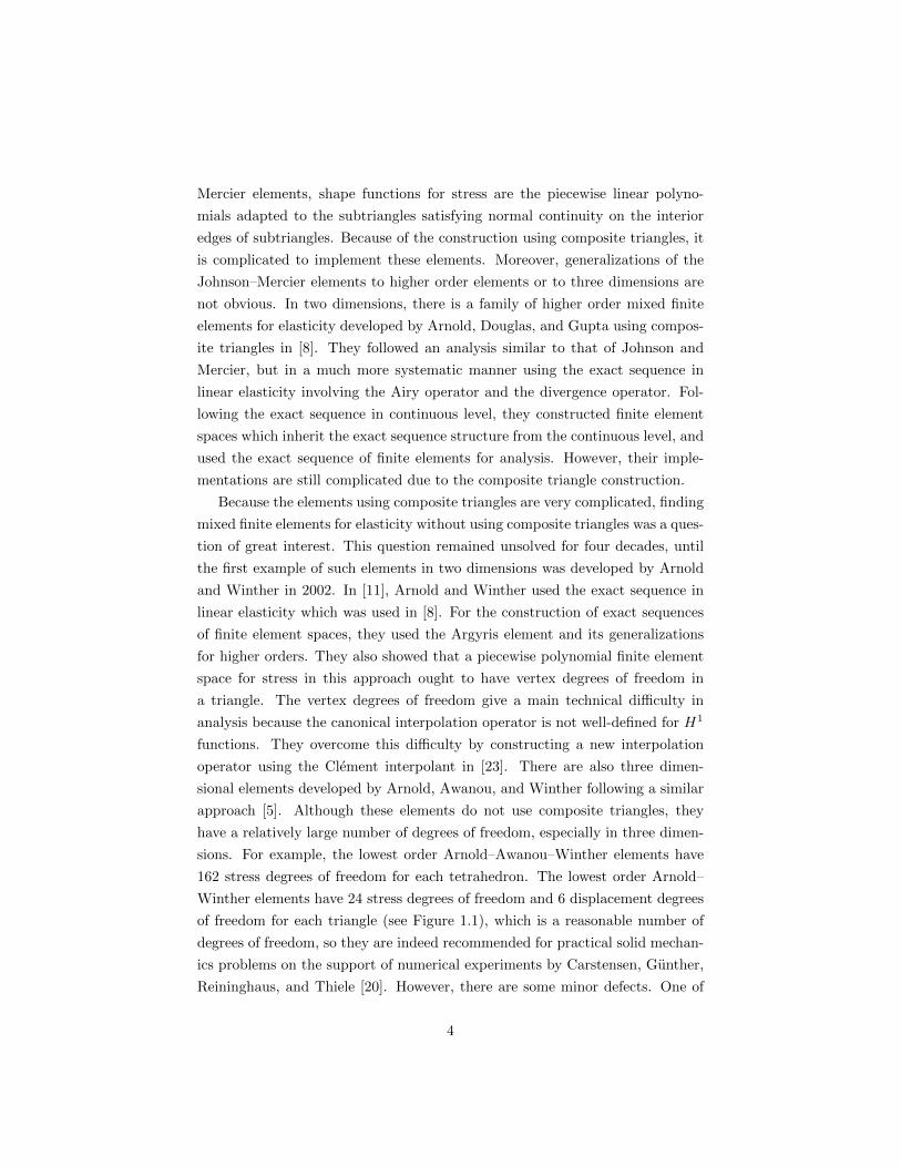
162 stress degrees of freedom for each tetrahedron. The lowest order Arnold–
Winther elements have 24 stress degrees of freedom and 6 displacement degrees
of freedom for each triangle (see Figure 1.1), which is a reasonable number of
degrees of freedom, so they are indeed recommended for practical solid mechan-
ics problems on the support of numerical experiments by Carstensen, Gunther,
Reininghaus, and Thiele [20]. However, there are some minor defects. One of
4

them is that the full approximability of the Arnold–Winther elements, which is
of order three for the lowest elements, is redundant when regularity of solutions
is low. Another defect is that the hybridization in [6] is not available because
of the vertex degrees of freedom.
Figure 1.1: Element diagrams for the lowest order stress, displacement of theArnold–Winther elements.
Figure 1.2: Element diagrams for the lowest order stress, displacement, androtation elements of the Arnold–Falk–Winther elements.
An alternative approach to mixed methods for elasticity is to impose symme-
try of stress weakly, by imposing orthogonality to spaces of skew-symmetric ten-
sors. From another point of view, we introduce a skew-symmetric tensor, which
is the Lagrange multiplier for the symmetry of stress, and rewrite the original
elasticity problems with the Lagrange multiplier. The Lagrange multiplier is
often called the rotation because it is the skew-symmetric part of the gradient
of displacement. Therefore, in this approach, we have three unknowns, i.e., the
stress tensor, the displacement vector, and the rotation. Historically, this weak
symmetry idea was firstly suggested by Fraeijs de Veubeke in [26] and extended
for higher orders by Amara and Thomas. The work of Amara and Thomas was
not exactly written in a modern context of finite element methods1, however,
they observed and explained crucial concepts and ideas with a careful analysis.
1They did not use standard terminologies in finite element methods such as finite elementspaces, stability, degrees of freedom, shape functions, and the inf-sup condition.
5

In [3], Amara and Thomas used a matrix-valued H(div) piecewise polynomial
space for stress and a piecewise discontinuous polynomial space for rotation.
Instead of a piecewise polynomial space for displacement, they used a piecewise
polynomial space on edges which may correspond to the trace of displacement.
For existence of numerical solutions, they used some additional terms for stress
using bubble functions and proved error estimates using an interpolation map.
The first finite elements of weak symmetry idea, described in mixed methods
context, is the PEERS elements developed by Arnold, Brezzi, and Douglas in
[7]. In the construction of PEERS elements, the vector-valued lowest order
Raviart–Thomas elements augmented with additional terms using the bubble
function, piecewise constants, and skew-symmetric piecewise linear functions are
used for the shape functions for stress, displacement, and rotation, respectively.
Following the weak symmetry idea and the approach of the PEERS elements,
Stenberg constructed new finite elements in two and three dimensions and also
for higher orders [47]. For displacement, he used the vector-valued discontinuous
polynomials as in the PEERS elements. However, he used different spaces for
stress and rotation. Instead of the Raviart–Thomas elements with additional
terms using the bubble function and continuous skew-symmetric spaces, which
were used in the PEERS elements, he used the Brezzi–Douglas–Marini–Nedelec
elements with additional terms using bubble functions for the stress and dis-
continuous polynomials for the rotation such that both of them have one higher
order approximation properties than the space for the displacement. He also
observed that a postprocessing is eligible for the numerical solution for displace-
ment, so a new numerical solution for displacement can be obtained, which has
as same accuracy as the ones for stress and rotation. He also claimed that new
finite elements using the Raviart–Thomas elements can be constructed with
similar arguments straightforwardly. There are other extensions of the PEERS
elements, done by Morley, to two dimensions for one higher order and to three
dimensions. She used the Raviart–Thomas–Nedelec elements with additional
terms using bubble functions as shape functions for stress, but she used non-
conforming finite elements for rotation to avoid vertex degrees of freedom. She
also observed the eligibility of postprocessing for the numerical displacement
as Stenberg did. In [10], Arnold, Falk, and Winther introduced an exterior
calculus framework for the study of mixed finite elements for elasticity. The
framework is based on the elasticity complex which is constructed from the
de Rham complex using the Bernstein–Gelfand–Gelfand resolution in represen-
tation theory by Eastwood [29]. As an application of the elasticity complex,
6

Table 1.1: Mixed finite elements for elasticity with triangular meshes. The σ,u, r denote the stress, the displacement, and the rotation, respectively. For allthe finite elements that k is involved, we assume k ≥ 1.
elements symmetryorder of error
mesh & dimensionσ u r
JM [36] strong 2 2 – composite, 2D
ADG [8] strong k + 2 k + 1 – composite, 2D
AW [11] strong k + 2 k + 1 – 2D
AAW [5] strong k + 2 k + 1 – 3D
AT [3] weak k – – 2D
PEERS [7] weak 1 1 1 2D
Stenberg I [47] weak k + 1 k k + 1 2D, 3D
Morley [40] weak 2 2 2 2D, 3D
AFW [10] weak k k k 2D, 3D
CGG [24] weak k + 1 k k + 1 2D, 3D
GG [32] weak k + 1 k k + 1 2D, 3D
JM = Johnson–Mercier, ADG = Arnold–Douglas–Gupta, AW = Arnold–Winther,
AAW = Arnold–Awanou–Winther, AT = Amara–Thomas,
AFW = Arnold–Falk–Winther, CGG = Cockburn–Gopalakrishanan–Guzman,
GG = Gopalakrishnan–Guzman
they developed the Arnold–Falk–Winther elements. In the analysis, they used
the elasticity complex to construct exact sequences of finite element spaces and
constructed an interpolation operator with a commuting property. The Arnold–
Falk–Winther elements are defined in two and three dimensions and for higher
orders with simple descriptions (see Figure 1.2), and have small numbers of
degrees of freedom. After this pioneering work, other elements were developed
following the analysis of same exterior calculus framework. For example, Cock-
burn, Gopalakrishnan, and Guzman constructed a family of elements such that
the finite element spaces for stress are based on the Raviart–Thomas–Nedelec
elements with additional terms using bubble functions [24]. These elements are
similar to Stenberg’s ones but have smaller degrees of freedom for same accuracy
of errors. They also showed that the hybridization is available for their elements.
More recently, another family of elements was developed by Gopalakrishnan and
Guzman [32], which have fewer degrees of freedom than their previous elements
with same accuracy of errors. We refer Table 1.1 for some features of these
elements.
There are also rectangular and quadrilateral mixed finite elements for elas-
ticity with both strong and weak symmetry. For strong symmetry elements,
7

Table 1.2: Mixed finite elements for elasticity with rectangular or quadrilateralmeshes. The σ, u, r denote the stress, the displacement, and the rotation,respectively. For all the finite elements that k is involved, we assume k ≥ 1.
elements symmetryorder of error
mesh & dimensionσ u r
JM [36] strong 2 2 – composite, quad., 2D
ADG [8] strong k + 2 k + 1 – composite, quad., 2D
PS [41] strong3/2 3/2 – rect., 2D
2 2 – composite, rect. 2D
Stenberg II [46] strong2 3 –
rect., 2D3 4 –
BJT [15] strong k k – rect., 2D, 3D
AA [4] weak k k k rect., 2D
Morley [40] weak 2 2 2 rect., 2D
Awanou [13] weak k k k rect., 2D, 3D
JM = Johnson–Mercier, ADG = Arnold–Douglas–Gupta, PS = Pitkaranta–Stenberg
AA = Arnold–Awanou, quad. = quadrilateral, rect. = rectangular
Johnson and Mercier constructed quadrilateral finite elements with linear poly-
nomials using composite quadrilaterals [36]. In [8], Arnold, Douglas, and Gupta
also constructed quadrilateral elements for higher orders using composite quadri-
laterals. Pitkaranta and Stenberg showed the error analysis of two mixed finite
elements in two dimensions [41]. Stenberg constructed some low order rectan-
gular mixed finite elements in two dimensions and showed error analysis in [46].
There is a family of rectangular elements in two and three dimensions and also
for higher orders developed by Becache, Joly, and Tsogka in [15]. For shape
functions for the stress and the displacement, they use the symmetric tensors
that each entry belongs to Qk+1, and the vectors that each entry belongs to Qk,
respectively, where Qk is the standard tensor product space of the polynomials
of degree less than or equal to k. To make the divergence operator is well-
defined on the finite element space for stress, they used a nonstandard choice
of degrees of freedom that each entry of the stress tensor is continuous along
specific one or two directions. Since the definition of degrees of freedom strongly
relies on the rectangular structure of meshes, it seems to be difficult to extend
their approach to triangular meshes. More recently, in [4], Arnold and Awanou
developed rectangular finite elements with strong symmetry in two dimensions
based on the idea of [11]. For weak symmetry elements, Morley constructed
rectangular elements in her generalization of the PEERS elements in [40]. In
[13], Awanou developed a family of rectangular elements with weak symmetry
8

in two and three dimensions and for higher orders. His elements have fewer
degrees of freedom than Morley’s ones. Some features of these elements are
summarized in Table 1.2. Rectangular elements are very useful for problems
with domains of special geometry, however, it is difficult to use them to the
problems which have general shape domains.
To summarize, after intensive studies of four decades, there are many mixed
finite elements for elasticity. Among them, the weak symmetry elements are
advantageous because they are defined in two and three dimensions and for
higher orders. Moreover, they have relatively simple descriptions with small
number of degrees of freedom.
1.3 Mixed methods for time dependent elastic-
ity and viscoelasticity
In continuum mechanics, there are many problems for which stress is of primary
interest. For example, to design and construct an earthquake resistant building,
the stress exerted on the building is one of most important quantities to consider.
Based on this philosophy, we use mixed finite element methods to study time
dependent problems of elasticity and viscoelasticity.
As we have seen in the previous section, mixed finite elements for elasticity
with weak symmetry have relatively few degrees of freedom and are relatively
easy to implement in both two and three dimensions. Thus we shall use the weak
symmetry elements for our studies of continuum mechanics problems. In this
section we briefly survey previous studies of elastodynamics and viscoelasticity
problems using mixed methods.
Mixed methods for linear elastodynamics have been studied by various re-
searchers. In [27], Douglas and Gupta used a displacement-stress formulation of
elastodynamics equations and the mixed finite elements using composite trian-
gles developed in [8]. For the error analysis of semidiscrete solutions, they use an
asymptotic expansion of solutions using the quasi-projection. As a consequence
of the error analysis, they showed that the errors for stress and displacement
are of same orders as for stationary elasticity problems. The superconvergence
result in their work is based on the superconvergence in the error analysis of
stationary problems but the error analysis for fully discrete solutions was not
shown. In [39], Makridakis proposed two approaches for linear elastodynamics,
the displacement-stress formulation used in [27] and a velocity-stress formula-
9

tion. The velocity-stress formulation is based on the work of Geveci for scalar
wave equations. In [31], Geveci suggested a velocity-flux formulation for scalar
wave equations and showed a unified error analysis for the Raviart–Thomas
and the Brezzi–Douglas–Marini elements. He also pointed out that a simi-
lar analysis can be adapted to the corresponding velocity-stress formulation of
elastodynamics. In the work of Makridakis, he only assumed that the finite
elements are stable, strongly symmetric, have a good approximability, and have
interpolation maps satisfying a certain commutativity property, so his analysis
is valid for many finite elements including the composite elements in [8, 36] and
the rectangular elements developed in [41, 46]. For the error analysis, Makri-
dakis used the elliptic projection approach, which was introduced in [49] for
heat equations. Using the elliptic projection, and an energy estimate, he sim-
plified the error analysis significantly than the one of Douglas and Gupta. He
also considered fully discrete solutions with general time discretization based
on the Pade approximation. In [15], Becache, Joly, and Tsogka constructed
new rectangular finite elements, which can be extended to three dimensions and
for higher orders, and applied them for linear elastodynamics. They used the
velocity-stress formulation and the elliptic projection for error analysis as in the
work of Makridakis.
Table 1.3: Comparison of the previous studies and the work in this thesisfor elastodynamics. (disp.-stress = displacement-stress, vel.-stress = velocity-stress) Finite elements are denoted by using the abbreviations in Table 1.1 andTable 1.2.
DouglasMakridakis
Becache this thesis
Gupta Joly Tsogka (chapter 3)
formulation disp.-stressdisp.-stress
vel.-stress vel.-stressvel.-stress
finite elements ADGJM, ADG, PS
BJT AFW, GGStenberg II
time scheme – Pade – Crank–Nicolson
In contrast to elastodynamics, there are not many previous works on mixed
methods for viscoelasticity. In [16], Becache, Ezziani, and Joly used their rect-
angular elements developed in [15] for the generalized Zener model of linear
viscoelasticity. To have a mixed form of equations, they took three unknowns,
the displacement, the total stress, and the difference of the total stress and the
elastic stress. Rewriting equations, a system of equations consisting of an al-
10

Table 1.4: Comparison of the previous studies and the works in the thesis forlinear viscoelasticity. (disp.-stress = displacement-stress, vel.-stress = velocity-stress) Finite elements are denoted by using the abbreviations in Table 1.1 andTable 1.2.
Becache Rognes this thesis
Ezziani Joly Winther (chapters 4, 5)
formulation disp.-stress vel.-stress vel.-stress
finite elements BJT AFW AFW, GG
viscoelastic model gZ qM& qKV M, KV, gZ
time scheme leap-frog type BDF2 Crank–Nicolson
symmetry of finite elements strong weak weak
M=Maxwell, KV=Kelvin–Voigt, gZ=generalized Zener, q=quasistatic
gebraic equation, and equations with one and two time derivatives. For time
discretization, they chose a leap-frog type scheme and proved that the scheme
is stable when a certain CFL condition holds. Some discussions on mass lump-
ing, PML adaptation, and upper bounds of CFL condition were presented. In
[44], Rognes and Winther studied mixed methods for the Kelvin–Voigt and the
Maxwell models of linear viscoelasticity but for quasistatic problems, i.e., the
problems that mass densities are vanishing. They suggested a unified framework
for general viscoelasticity models and applied it to the specific two problems.
A key idea of the unified framework is using two stresses, the viscous and the
elastic ones, and generalize the velocity-stress formulation for elastodynamics
in the context of viscoelasticity equations. For mixed finite elements, they used
the Arnold–Falk–Winther elements and a variant of them for the lowest order
by Falk. Due to the weak symmetry of finite elements, the equations of the
Maxwell and the Kelvin–Voigt models had to be rewritten in weak symmetry
form. They used the skew-symmetric part of the gradient of velocity as the
Lagrange multiplier for symmetry of stress, and obtained differential algebraic
equations for the semidiscrete solutions. For full discretization, they used the
second backward differentiation formula and applied a known result in general
theory of the numerical analysis of differential algebraic equations for conver-
gence. They also presented numerical results for the Zener model.
1.4 Overview of chapters
The organization of this thesis is as follows.
11

In chapter 2, we develop background materials which will be needed in the
rest of this thesis. We present notations, definitions, a brief survey of mixed
methods, and expository descriptions of the Arnold–Falk–Winther (AFW) and
the Gopalakrishnan–Guzman (GG) elements, which we will use in our studies.
We revisit improved error estimates and postprocessing results, proposed in
[47, 35, 10] for these two families of elements with complete proofs. We also
introduce some results on evolutionary equations and regularity of functions,
that we need in later chapters, with their complete proofs.
In chapter 3, we study mixed methods for linear elastodynamics, which rep-
resents wave propagation in elastic media, using a velocity-stress mixed formu-
lation. This is the first work of mixed methods for elastodynamics using weak
symmetry elements. We use the Crank–Nicolson scheme for time discretization
and propose error bounds by a priori error analysis. A key idea for the error
analysis is our weakly symmetric elliptic projection which will be explained in
chapter 2. By a careful analysis, we can obtain error bounds in elastodynamics,
similar to the ones in stationary elasticity problems, using the AFW and GG
elements. We also prove that robustness for nearly incompressible materials still
holds in elastodynamics. Some numerical results which support our analysis are
presented at the end of this chapter.
In chapter 4, we consider mixed methods for the Kelvin–Voigt model of linear
viscoelasticity, which is a fundamental unit to construct models of viscoelastic
solids. We study the full dynamic Kelvin–Voigt model with a nonvanishing
mass density using a velocity-stress mixed formulation, the AFW and GG ele-
ments, and the Crank–Nicolson scheme for time discretization. The semidiscrete
problem of the Kelvin–Voigt model leads to a system of differential algebraic
equations, so initial data for numerical computation should be carefully chosen
to achieve stability of time discretization. We show an error analysis for fully
discrete solutions and propose error bounds. There are also numerical results
which support our error analysis.
In chapter 5, we consider mixed methods for the Maxwell and the general-
ized Zener models of linear viscoelasticity. Since the Maxwell and the Zener
models can be written in a unified form and the Maxwell model is a special case
of the Zener model, we show careful error analysis only for the Zener model.
Extending the analysis to the generalized Zener model is straightforward. As in
elastodynamics and the Kelvin–Voigt model problems, we use a velocity-stress
formulation, the AFW and GG elements, and the Crank–Nicolson scheme for
time discretization. We show that the error bounds of our numerical scheme are
12

stable as the parameters, which determine viscoelastic features of the material,
decays to zero. As a consequence, our numerical algorithm can be used for a
material which is a composition of elastic and viscoelastic solids. Another ben-
efit of our method is that no time integration is needed in the computation of
each time step. Based on the displacement, the solution of Zener model includes
a convolution term with a kernel depending on material parameters and time
(see e.g., [37]), so a numerical solution also needs a numerical time integration
for all the past time intervals at each time step. In mixed methods using our
velocity-stress formulation, the equations of the Zener model is written as dif-
ferential equations (see e.g., [16, 33]), henceforth no numerical time integration
is required and an implementation of the algorithm is easier. The payment for
these advantages is a larger system of equations. However, the number of de-
grees of freedom increases almost linearly to the number of mesh components,
i.e, the triangles, the edges, and the vertices. Since the computational cost in-
creases linearly on the number of degrees of freedom in advanced linear algebraic
solvers, the increment of computational cost is not a big obstacle. In contrast
to this, the number of time intervals for numerical integration is not limited
and therefore the computation cost for numerical integration can be very large
unless there is a good argument to justify that a truncation of the time interval
for numerical integration is reasonable. As in previous chapters, we present
numerical results supporting our error analysis.
Finally, in chapter 6, we show numerical results which are more interesting
from the physical point of views. In elastodynamics, there are examples showing
that the different material parameters influence differently on the propagation
of P and S waves in homogeneous and heterogeneous isotropic media. We also
present numerical results which show wave propagation in anisotropic media. In
viscoelasticity, we use our numerical schemes for creep compliances of viscoelas-
tic materials. We present a simple schematic model which compares reflected
waves in a purely elastic medium and a medium including viscoelastic regions.
13

Chapter 2
Preliminaries
In this chapter, we will survey preliminary backgrounds for our discussions in the
rest of this dissertation. The contents of this chapter are organized as follows.
In section 2.1, we introduce notations and definitions. In section 2.2, we
survey continuum mechanics backgrounds which are necessary to derive our
governing equations later. In section 2.3, we introduce a general theory of
mixed finite element methods. In section 2.4, we survey mixed methods for
linear elasticity and introduce two families of mixed finite elements for elasticity.
For those families, we present some technical details including a priori error
estimates, robustness for nearly incompressible materials, postprocessing, and
the existence of an elliptic projection which preserves weak symmetry. Finally, in
section 2.5, we prove miscellaneous lemmas which are needed for error estimates
and regularity of weak solutions.
2.1 Notations and definitions
Let Ω be a bounded smooth domain in Rn with n = 2 or 3. If a range is
not specified, then indices i, j span 1, · · · , n. We use ∂i to denote the partial
derivative for the i-th variable in Rn.
We use V and M to denote Rn and Rn×n. We also use S and K to denote
the spaces of symmetric and skew-symmetric n × n matrices, respectively. For
σ : Ω → M and u : Ω → V, their components are denoted by σij and ui,
14

respectively. Let us define
(σ, τ) =
∫Ω
σ : τ dx :=
∫Ω
∑i,j
σijτij dx,
(v, w) =
∫Ω
v · w dx :=
∫Ω
∑i
viwi dx,
for σ, τ : Ω → M and v, w : Ω → V. It is easy to check that these are inner
products. We can define norms by ‖σ‖2 = (σ, σ), ‖u‖2 = (u, u) and define two
Hilbert spaces
L2(Ω;M) = σ : Ω→M | ‖σ‖ <∞, L2(Ω;V) = u : Ω→ V | ‖u‖ <∞.
For σ : Ω → M and u : Ω → V, div σ and gradu are defined by the row-wise
divergence and the row-wise gradient
div σ =∑j
∂jσij , (gradu)ij = ∂jui,
respectively, where ∂jσij , ∂jui are understood in the sense of distributions [45].
For σ : Ω→M, the symmetric and skew-symmetric parts of σ are
symσ =σ + σT
2, skw σ =
σ − σT
2,
where σT is the transpose of σ. If σ : Ω → M and div σ ∈ L2(Ω;V), we define
‖σ‖2div = ‖σ‖2 + ‖ div σ‖2 and for a subspace X of M,
H(div,Ω;X) = σ ∈ L2(Ω;X) | ‖σ‖div <∞.
We also define function spaces M , S, V , and K by
M = H(div,Ω;M), S = H(div,Ω;S),
V = L2(Ω;V), K = L2(Ω;K).(2.1)
For a nonnegative integer 0 ≤ m < ∞, we use Cm(Ω) to denote the set of
functions defined on Ω such that the functions and all their partial derivatives
of order less than or equal to m are continuous and can be continuously extended
to Ω. We use C∞(Ω) to denote the intersection of all Cm(Ω) for m ≥ 0. We
also use Cm0 (Ω) to denote the functions in Cm(Ω) whose supports are compact
15

sets in Ω.
A multi-index α is a sequence of nonnegative integers (α1, · · · , αn) and the
degree of α, denoted by |α|, is defined by |α| := α1 + · · ·+ αn. For u ∈ Cm(Ω),
we define
‖u‖2m =∑|α|≤m
‖∂αu‖2, where ∂αu := ∂α11 · · · ∂αn
n u.
The Sobolev space Hm(Ω) is the Banach space which is the completion of Cm(Ω)
with the norm ‖ · ‖m. We define H1(Ω) as the closure of C∞0 (Ω) in H1(Ω) and
it becomes a subspace of H1(Ω). For X = V,M,K, or S, Hm(Ω;X) is the space
of X-valued functions such that each component of the function is in Hm(Ω). If
X is clear in context, Hm(Ω) is used as an abbreviation of Hm(Ω;X).
For a Banach space X and 0 < T0 < ∞, C0([0, T0];X ) denotes the set of
functions f : [0, T0] → X which are continuous in t ∈ [0, T0]. For an integer
m ≥ 1 we define
Cm([0, T0];X ) = f | ∂lf/∂tl ∈ C0([0, T0];X ), 0 ≤ l ≤ m,
where ∂lf/∂tl is the l-th time derivative in the sense of the Frechet derivative in
X (see e.g., [50]). For a function f : [a, b]→ X , we define the space-time norm
‖f‖Lp([a,b];X ) =
(∫ b
a‖f‖pX dt
)1/p
, 1 ≤ p <∞,
ess supt∈[a,b] ‖f‖X , p =∞.
If the time interval is fixed as [0, T0], then we use LpX to denote Lp([0, T0];X )
for simplicity. We define the space-time Sobolev spaces Wm,p([0, T0];X ) for
nonnegative integer m and 1 ≤ p ≤ ∞ as the closure of Cm([0, T0];X ) with
the norm ‖u‖Wm,pX =∑ml=0 ‖∂lu/∂tl‖LpX . We adopt a convention ‖f, g‖X
to denote ‖f‖X + ‖g‖X for the norm of a Banach space X . For simplicity of
notations, f is used to denote the time derivative of f and similarly, f ,...f are
used to denote ∂2f/∂t2, ∂3f/∂t3, respectively.
For a triangle or a tetrahedron T , a vector space X, and a nonnegative integer
k, Pk(T ;X) is the space of X-valued polynomials defined on T of degree less than
or equal to k. If T is a triangle, the space Nk(T ), k ≥ 1 is
Nk(T ) = Pk−1(T ;R2) + (−wx2, wx1) |w ∈ Pk−1(T ), (2.2)
16

which is the usual space of shape functions for the (rotated) Raviart–Thomas
elements [9, 42]. We define Nk(T ) as the space consisting of all τ in Pk(T ;R2×2)
such that each row of τ is in Nk(T ). We will use this space when we define the
degrees of freedom for our mixed finite elements for elasticity in section 2.4.2.
For the domain Ω, Th denotes a shape-regular quasi-uniform triangulation
of Ω for which the maximum diameter of triangles (or tetrahedra) is h. For an
integer k ≥ 0 and a vector space X, Pk(Th;X) is the space of piecewise X-valued
polynomials adapted to Th of degree less than or equal to k. If X is a subspace
of M, then Pk(Th,div;X) = Pk(Th;X) ∩H(div,Ω;X).
Let ∆t > 0 such that T0 = N∆t for an integer N , and tj = j∆t for j =
0, 1, · · · , N . For a continuous function f defined on [0, T0], we define f j = f(tj)
and f j+1/2 = f(tj + ∆t/2). For example, σj , σP,jh , eP,jσ denote σ(tj), σPh (tj),
ePσ (tj) for the functions σ, σPh , ePσ defined on [0, T0], respectively. For a sequence
f jj≥0, we define
∂tfj+ 1
2 =f j+1 − f j
∆t, f j+
12 =
f j + f j+1
2,
∂2t f
j =f j+1 − 2f j + f j−1
∆t2.
(2.3)
Note that for f defined on [0, T0], f j+1/2 6= f j+1/2 in general.
2.2 Continuum mechanics
We survey basic continuum mechanics which is necessary to derive the governing
equations of our problems.
Continuum mechanics is a way to formulate kinematic behavior of materials
mathematically. In continuum mechanics, a material body is regarded as a
continuum and the microscopic structures of the material are neglected. In
many macroscopic scale problems, it is a good approximation of real physical
phenomena.
2.2.1 Deformation, strain, momenta, and stress
If a continuum body occupies a bounded domain in Rn where n = 2, 3, then
the occupied domain is called a configuration. For simplicity, we assume all
configurations have sufficiently smooth boundaries. Let Ω be the domain that
a continuum body occupies at initial state, which is called the reference config-
17

uration. The deformation map Φ : Ω × [0, T0] → Ω′ ⊂ Rn is a map which is
continuously differentiable, homeomorphic, and orientation preserving. The im-
age of Ω under Φ(·, t) for t ∈ [0, T0] is called the deformed configuration at time t
and denoted by Ωt. The gradient of deformation map is called the deformation
gradient and denoted by F .
The rigid deformations are the deformation maps of the form x 7→ A(t)x+b(t)
for x ∈ Rn where t 7→ A(t), t 7→ b(t) are continuous maps to the space of
orthogonal matrices of positive determinant and the space Rn, respectively. In
continuum mechanics, rigid deformations are not interesting because when a
deformation map is a rigid deformation, all kinematic quantities of deformed
configuration are obtained by composing the inverse of the rigid deformation
and the corresponding kinematic quantities of reference configuration. A C1
deformation map Φ is a rigid deformation if and only if FTF = I (see [22],
p. 44), so we call (FTF − I)/2 the (Green–St.Venant) strain or strain tensor
where I is the identity matrix in Rn×n.
In many problems, it is convenient to work with the difference of the de-
formed and reference configurations rather than the deformed configuration it-
self. The displacement u : Ω→ Rn is defined by u(x, t) = Φ(x, t)− x for x ∈ Ω,
t ∈ [0, T0]. Then the gradient of displacement is gradu = F − I and the strain
tensor can be written
1
2(FTF − I) =
1
2((gradu+ I)T (gradu+ I)− I)
=1
2((gradu)T (gradu) + (gradu)T + gradu). (2.4)
We use v to denote ∂u/∂t, the velocity field and ρ(x) to denote the mass density
at x ∈ Ω. Then the linear momentum and angular momentum (about the origin)
on a subregion ω are defined by∫ω
ρv dx,
∫ω
ρ~x× v dx,
where ~x is the position vector defined by the coordinate x. If n = 2, we can
still define the angular momentum by extending all two dimensional vectors to
three dimensional ones which have zero third coordinate.
We now consider an internal surface force on a surface in a continuum body.
For a surface in a continuum body, there is a force acting between two continuum
subbodies along the surface. In a continuum sense, this force is proportional to
18

surface area, and at a point on the surface it is defined as the limit of force on
shrinking surface regions divided by the surface area of the regions. We call this
internal surface force as the stress vector or traction.
Let ω0, ω1 be two subregions in a continuum body Ω with contacting surface
S. If we let ν be the unit normal vector of S at point x which is outward from
ω0, then the surface force that ω0 exerts on ω1 at x is denoted by T (x, ν) ∈ Rn.
Thus, the surface force that ω1 exerts on ω0 at x is T (x,−ν), and T (x,−ν) =
−T (x, ν) by Newton’s third law of motion.
We assume that the balance laws of linear and angular momenta, which are
d
dt
∫ω
ρv dx =
∫∂ω
T (x, ν) dS +
∫ω
f dx,
d
dt
∫ω
ρ~x× v dx =
∫∂ω
~x× T (x, ν) dS +
∫ω
~x× f dx,
hold for any subregion ω ⊂ Ωt, where ν is the outward unit normal vector field
on ∂ω and f is a body force. Here we state an important result on stress vectors
which was proved by Cauchy. For its proof, see [34], chapter 5.
Theorem 2.1 (Cauchy’s theorem). If the balance laws of linear and angular
momenta hold, then there exists a matrix valued function σ from Ωt to S such
that T (x, ν) = σ(x)ν for all x ∈ Ωt where the right-hand side is the matrix-vector
multiplication.
The σ in the Cauchy’s theorem is called the (Cauchy) stress tensor or simply
stress. In the proof of the above theorem, the symmetry of the stress tensor is
due to the balance law of angular momentum.
Let ω be a subregion of Ω and f be an external body force acting on ω. By
the divergence theorem, ∫∂ω
σν dS =
∫ω
div σ dx.
Thus the integration of surface traction exerted to ω on ∂ω is same as the
force obtained by integrating −div σ on ω. By using the balance law of linear
momentum, conservation of mass, the fact that ω is arbitrary, we have
d
dt(ρv)− div σ = f in Ω.
We refer to [34] for derivation of the above equation.
19

2.2.2 Linear elasticity
A material is called elastic if its stress tensor at a certain time is solely deter-
mined by the deformed configuration at that time. From a physical point of
view, a key feature of elastic materials is that the shape of material deformed
by a stress vector returns to the original shape when the stress vector which
caused deformation is removed. In an elastic material, the stress and strain ten-
sors satisfy a relation determined by the kinematic properties of the material.
This relation governing kinematic behavior of a material is called a constitutive
law.
We confine our discussion to elastic materials for which the constitutive
laws are linear equations relating the stress and strain tensors, and we also use
the linearized strain tensor, which is the linear approximation of strain tensor,
instead of the original one. These linearization assumptions are acceptable in
many applications when deformations of material are relatively small compared
to the scale of whole kinematic system.
From the definition of strain tensor in (2.4), the linearized strain tensor
ε = ε(u) : Ω→ S is defined by
ε(u) =1
2(gradu+ (gradu)T ), i.e., εij =
1
2(∂iuj + ∂jui), 1 ≤ i, j ≤ n,
for given displacement u : Ω→ V.
From our assumption that the constitutive equations are linear, the stress
tensor σ and the linearized strain tensor ε(u) are related by
σ(x) = C(x)(ε(u)(x)), (2.5)
where C(x) : S→ S is symmetric positive definite and uniformly bounded above
and below. The stiffness tensor or elasticity tensor C is a rank 4 tensor with
components Cijkl : Ω→ R, 1 ≤ i, j, k, l ≤ n such that
Cijkl = Cjikl = Cklij , (2.6)
which may be determined by measuring the kinematic properties of elastic
medium with experiments. For simplicity, the stress-strain relation (2.5) will
be denoted by σ = Cε(u). From the uniform boundedness of C(x), the map
C : L2(Ω;S)→ L2(Ω;S) is a symmetric positive definite bounded linear opera-
tor.
20

The compliance tensor A(x) is defined by A(x) = C(x)−1. Thus A(x) : S→ Sis symmetric positive definite and uniformly bounded above and below. An
elastic medium is called isotropic if kinematic properties of the material at each
point is same in any direction. If an elastic medium is isotropic, then Cτ and
Aτ have the forms
Cτ = 2µτ + λ tr(τ)I, Aτ =1
2µ
(τ − λ
2µ+ nλtr(τ)I
), (2.7)
where µ, λ are positive scalar functions defined on Ω, called the Lame coeffi-
cients, and tr(τ) is the trace of τ .
2.2.3 Linear viscoelasticity
Viscoelastic materials
In constitutive laws of elastic materials, the time dependence of strain is not
involved. However, in many fluids the stress tensor is related to the strain rate
tensor, which is the time derivative of strain tensor. Such a dependence is called
viscosity of materials.
A material is called viscoelastic if the material has both elastic and viscous
kinematic features. Many polymers, biomedical tissues, and geophysical materi-
als are viscoelastic, so it is important to understand the behavior of viscoelastic
materials in science and engineering.
In order to model viscoelastic materials, we need a constitutive law which
describes the relation of stress, strain, and strain rate tensors. If we confine
our attention to linear viscoelastic materials, then there is a unified framework
to describe all possible constitutive laws by using convolution integrals in time
with some kernels. This integral form to describe constitutive laws, called the
hereditary approach, is useful for analysis from the viewpoint of PDE but it
creates difficulties for numerical computation because the numerical time inte-
gration of convolution is not easy to implement in an efficient way. Therefore
we shall use differential forms of constitutive laws, say differential constitutive
laws, for our study of numerical methods for viscoelasticity problems. The dif-
ferential constitutive laws are not available for all linear viscoelastic materials.
Some materials need constitutive laws with fractional time derivatives, which
are not local operators and cannot be written as differential operators [14].
However, differential constitutive laws are obtained for the mechanical models
of viscoelastic materials, which will be introduced later, and mechanical models
21

include many important models of viscoelastic materials. The equivalence of
integral and differential forms of constitutive laws under some assumptions is
discussed in [33].
Hereditary approach
We briefly introduce the hereditary approach because it is related to the two
fundamental characteristics of viscoelastic materials, the creep compliance and
the relaxation modulus.
Before we define the creep compliance and relaxation modulus mathemati-
cally, let us describe those properties in a physical sense. If a material is purely
elastic, then the dependence of strain on stress is instantaneous and strain is not
changed as long as stress is constant in time. However, in viscoelastic materials,
the dependence is not instantaneous and strain changes in time even if stress is
held constant. We can see it clearly when we push a foam pillow with a force
which is constant in time. This kinematic behavior is called creep. Conversely,
suppose we push an elastic material, deform it up to a certain distance, and then
keep the state. The stress response remains constant. In viscoelastic materials,
when we do the same action, the stress is the strongest at the beginning moment
and decays in time. This is explained by the fact that the molecules of viscoelas-
tic material are rearranged by stress and the rearrangement of molecules requires
some time. This kinematic behavior is called relaxation.
Now, in a one dimensional model, we introduce rigorous definitions of the
creep compliance and relaxation modulus and describe the hireditary approach
of linear viscoelasticity. Let σ(t) be the stress and ε(t) be the linear strain,
which are scalars in the one dimensional case. For constitutive laws, we assume
invariance of time translation and causality of material properties. Invariance
of time translation means if the input at certain time t0 induces output at time
t0 + δ, δ > 0, then the same input at time t0 + d induces the output at time
t0 + d + δ which is same as the output at time t = t0 + δ. Causality is the
property that the output at time t1 is completely determined by the inputs in
the time range t ≤ t1.
Let Θ(t) be the Heaviside function, i.e., the function defined on R which is
1 for t > 0 and 0 for t < 0. The creep test is to set σ(t) = Θ(t) and observe
the corresponding ε(t) which is called the creep compliance and is denoted by
J(t). The relaxation test is to set ε(t) = Θ(t) and observe the corresponding
σ(t) which is called the relaxation modulus and is denoted by G(t). These two
22

functions are called materials functions. From causality, J(t) = G(t) = 0 for
t < 0. In experiments, G, J ≥ 0 (or symmetric positive definite in higher than
one dimension) and on 0 < t < +∞, J is non-decreasing andG is non-increasing.
Suppose J(t) is differentiable and increasing in time. Then for t > 0, J > 0 and
0 ≤ J(0+) < J(t) < J(+∞) ≤ +∞. Similarly, under the assumption G < 0,
+∞ ≥ G(0+) > G(t) > G(+∞) ≥ 0.
By using the material functions, the stress and strain are described by the
Riemann–Stiltjes integrals
ε(t) =
∫ t
−∞J(t− τ)dσ(τ), σ(t) =
∫ t
−∞G(t− τ)dε(τ).
They are called creep and relaxation representations, respectively. The above
formulas are justified by the Boltzmann superposition principle which will be
explained below.
Suppose a constant amount of stress σ1 is exerted from time τ1, i.e., σ(t) =
σ1Θ(t − τ1). Then the corresponding strain ε(t) is σ1J(t − τ1). Suppose the
stresses ∆σi = σi+1−σi are added at time τi for i = 2, · · · , n. τ1 < τ2 < · · · < τn.
Then the strain is ε(t) =∑ni=1 ∆σiJ(t−τi). In this manner, for continuous σ(t),
the corresponding strain is obtained as the limit of the summation by increasing
n and letting the maximum of time intervals converge to zero. In a similar way,
the formula of σ(t) is obtained.
Mechanical models
In mechanical models, a viscoelastic material is understood as a continuum of
infinitesimal elements consisting of a combination of infinitesimal springs and
dashpots. For example, the special case of a linear elastic material is modeled
by a continuum of elements consisting of infinitesimal springs. In a mechanical
model of viscoelastic materials, for each spring and dashpot unit, the elastic
stress σe and viscous stress σv are related to the strain tensor and strain rate
tensor by
σe = Cε(u), σv = C ′ε(u), (2.8)
where C and C ′ are rank 4 tensors satisfying (2.6) and are uniformly bounded
from above and below. By combining spring and dashpot units in series or par-
allel, we can make infinitely many mechanical models of viscoelastic materials.
23

In Figure 2.1, we illustrate the spring-dashpot combination of some elemen-
tary models. The Kelvin–Voigt and Maxwell models are obtained by combining
one spring and one dashpot in parallel and in series, respectively. The Zener
model is the parallel combination of Maxwell component and one spring, and
the generalized Zener model is a generalization of Zener model with multiple
Zener components.
Figure 2.1: Examples of mechanical models of viscoelastic materials. TheKelvin–Voigt, Maxwell, Zener (or standard linear solid), and generalizedMaxwell (or Weichert) models.
In the Kelvin–Voigt model, the elastic and viscous stresses σe, σv, are related
to ε(u) and ε(u) by the spring and dashpot units as σe = Cε(u), σv = C ′ε(u).
The total stress is the sum of elastic and viscous stresses, so a constitutive
equation is
σ = Cε(u) + C ′ε(u).
In the Maxwell model, we consider the decomposition of displacement u =
ue + uv where ue and uv are the parts of displacement involved with the spring
and dashpot units. By (2.8), the stresses related to the spring and dashpot
components are Cε(ue) and C ′ε(uv). However, by Newton’s third law, Cε(ue) =
C ′ε(uv), which is the total stress tensor σ. If we let A = C−1, A′ = C ′−1, then
Aσ = ε(ue), A′σ = ε(uv). Thus a constitutive equation for the Maxwell model
is
Aσ +A′σ = ε(ue) + ε(uv) = ε(u).
The constitutive equations of the Zener and the generalized Zener models are
obtained with similar arguments. The derivation of equations of the Zener model
will be discussed in detail in Chapter 5. A similar approach can be applied to
the generalized Maxwell and generalized Zener models.
Before moving to the next section, we remark that the viscoelastic features
of one material can be described by more than one mechanical models, i.e., two
24

different mechanical models may show kinematics of exactly same creep compli-
ance and relaxation modulus. For instance, there is another description of the
Zener model (see [48]), which is the serial combination of one Kelvin–Voigt com-
ponent and a spring. In the hereditary approach, we have a unique constitutive
law for given creep compliance and the relaxation modulus. However, as we
have seen in the examples of the Maxwell and Kelvin–Voigt models, differential
constitutive laws include quantities which are strongly motivated by the struc-
ture of mechanical models which may not be intrinsic in the sense of physics.
The differential constitutive laws from different mechanical models may have
very different forms of equations nonetheless they describe same kinematic fea-
tures. In our study of the Zener model, we use the generalized Maxwell form of
mechanical model because it is easier to analyze than the model of generalized
Kelvin–Voigt form even if they have same kinematic features.
2.3 Mixed finite element methods
In this section, we introduce basics of saddle point problems and mixed finite
element methods. For more information about mixed finite element methods,
see [19].
2.3.1 Saddle point problems
Let Σ, V be Hilbert spaces and suppose that a : Σ × Σ → R, b : Σ × V → Rare bounded bilinear forms. We denote the dual spaces of Σ, V by Σ∗, V ∗. We
now consider a variational problem with constraints.
Constrained minimization problem. For F ∈ Σ∗, G ∈ V ∗, find σ ∈ Σ
which minimizes
J(σ) =1
2a(σ, σ)− F (σ),
subject to the constraint b(σ, v) = G(v) for all v ∈ V .
Instead of this minimization problem, we find a critical point (σ, u) ∈ Σ×Vof
L(τ, v) =1
2a(τ, τ) + b(τ, v)− F (τ)−G(v), (τ, v) ∈ Σ× V, (2.9)
by using the Lagrange multiplier u. By the Frechet derivative computation, we
25

see that a critical point (σ, u) of (2.9) should satisfy
a(σ, τ) + b(τ, u) = F (τ), τ ∈ Σ,
b(σ, v) = G(v), v ∈ V.(2.10)
Note that for any (τ, v) ∈ Σ× V , the inequalities
L(σ, v) ≤ L(σ, u) ≤ L(τ, u),
hold, so the variational problem of (2.9) is called a saddle point problem.
We will discuss necessary and sufficient conditions for the well-posedness of
problem (2.10). Define A : Σ→ Σ∗, B : Σ→ V ∗ by
(Aσ)(τ) = a(σ, τ), (Bσ)(v) = b(σ, v), τ ∈ Σ, v ∈ V.
Then we can rewrite (2.10) as(A B∗
B 0
)(σ
u
)=
(F
G
). (2.11)
In order to show well-posedness of (2.10), let
Z = τ ∈ Σ | b(τ, v) = (Bτ)(v) = 0, ∀v ∈ V , (2.12)
which is the null space of B. Since Z is a closed subspace of Σ, we have the
orthogonal decomposition Σ = Z + Z⊥, and Σ∗ = Z∗ + (Z⊥)∗. Let πZ∗ ,
πZ⊥∗ be the projections from Σ∗ onto Z∗, (Z⊥)∗, and define AZZ : Z → Z∗,
AZ⊥ : Z → (Z⊥)∗, A⊥Z : Z⊥ → Z∗, A⊥⊥ : Z⊥ → (Z⊥)∗ by
AZZ := πZ∗ A|Z , A⊥Z := (πZ∗A)|Z⊥ , (2.13)
AZ⊥ := (πZ⊥∗A)|Z⊥ , A⊥⊥ := (πZ⊥∗A)|Z⊥ .
The following theorem for the well-posedness of (2.10) was proved by Brezzi.
See [19] for its proof.
Theorem 2.2. Suppose that AZZ in (2.13) is an isomorphism and B is onto.
Then (2.10) has a unique solution (σ, u) ∈ Σ × V and there exists c > 0 such
26

that
‖σ‖Σ + ‖u‖V ≤ c(‖F‖Σ∗ + ‖G‖V ∗).
Remark 2.3. In the above theorem, the two conditions that AZZ is isomorphic
and B is onto, are called the first and second Brezzi conditions. Since b is a
bounded bilinear form, the second Brezzi condition is equivalent to the inf-sup
condition
inf06=v∈V
sup06=τ∈Σ
b(τ, v)
‖τ‖Σ‖v‖V≥ γ > 0, (2.14)
by the closed range theorem in functional analysis [50].
If the bilinear form a is symmetric, then the first Brezzi condition is obtained
from another inf-sup condition
inf0 6=σ∈Z
sup0 6=τ∈Z
a(σ, τ)
‖σ‖Σ‖τ‖Σ≥ γ′ > 0. (2.15)
Its proof is obtained by identifying Σ and Σ∗ by the Riesz representation theorem
and using the closed range theorem.
2.3.2 Mixed finite elements and Brezzi conditions
We will discuss the numerical solution of saddle point problems. Since the
bilinear form a is symmetric in most important problems, we assume that a is
symmetric for simplicity.
In order to solve the saddle point problems numerically with finite elements,
we use finite element spaces Σh ⊂ Σ, Vh ⊂ V and consider the following discrete
form of problem (2.10): Find (σh, uh) ∈ Σh × Vh such that
a(σh, τ) + b(τ, uh) = F (τ), τ ∈ Σh,
b(σh, v) = G(v), v ∈ Vh.(2.16)
The pair of finite element spaces (Σh, Vh) is called mixed finite elements and
the numerical methods of solving the discrete saddle point problem (2.16) with
mixed finite elements are called mixed finite element methods or mixed methods.
We consider the conditions that the problem (2.16) is well-posed. If we apply
Theorem 2.2 to (2.16), then we only need to check the first and second Brezzi
27

conditions for (Σh, Vh). Let
Zh = τ ∈ Σh | b(τ, v) = 0, v ∈ Vh. (2.17)
By the symmetry assumption of bilinear form a, as we pointed out in Remark
2.3,the Brezzi conditions are obtained from the two inf-sup conditions
inf0 6=σ∈Zh
sup0 6=τ∈Zh
a(σ, τ)
‖σ‖Σh‖τ‖Σh
≥ αh > 0, (2.18)
inf06=v∈Vh
sup06=τ∈Σh
b(τ, v)
‖τ‖Σh‖v‖Vh
≥ βh > 0. (2.19)
Let us consider a family of mixed finite elements (Σh, Vh)h>0 with parameter
h and suppose that there are αh, βh for each h. Then (Σh, Vh)h>0 is called
stable if αh, βh are bounded below by some positive constants independent
of h. For simplicity, we usually use (Σh, Vh) to denote the family of finite
elements (Σh, Vh)h>0. If (Σh, Vh) is stable, then the following quasi-optimal
error estimate is straightforwardly obtained from Theorem 2.2.
‖σ − σh‖Σ + ‖u − uh‖V ≤ c
(infτ∈Σh
‖σ − τ‖Σ + infv∈Vh
‖u− v‖V). (2.20)
2.4 Mixed finite elements for linear elasticity
with weak symmetry
From the balance law of angular momentum, the stress tensor is symmetric and
the symmetry of stress must be enforced when we find a numerical approxima-
tion of the stress. The symmetry of stress can be imposed on the numerical
solution strongly by using symmetric finite elements for stress. However, it is
not easy to find stable families of such mixed finite elements and they have a
fairly large number of degrees of freedom in general. This is a nontrivial draw-
back in practical computations. An alternative is to enforce symmetry of stress
weakly by requiring that σh, the numerical approximation of stress, to be or-
thogonal to a skew-symmetric finite element space. To our knowledge, this weak
symmetry idea firstly appeared in [26] and extended to higher orders in [3]. The
first finite elements in the context of mixed finite elements were the PEERS
elements developed in [7]. Thereafter, numerous mixed finite elements for linear
elasticity were developed with the weak symmetry idea [10, 17, 24, 32, 46, 47].
28

In general, this weak symmetry elements are easier to implement and have have
fewer degrees of freedom for low order elements than strong symmetry elements
[5, 8, 11, 36].
2.4.1 Mixed formulations of linear elasticity
In our discussions, we only consider problems with the homogeneous displace-
ment boundary conditions u = 0 on ∂Ω for simplicity but all discussions can be
extended easily to problems with inhomogeneous displacement boundary con-
ditions.
From the balance of linear momentum, − divCε(u) = f at equilibrium for
an external body force f ∈ V . In order for mixed formulations, we introduce
a new variable σ : Ω → S for the stress Cε(u) and have Aσ = ε(u). From the
homogeneous displacement boundary conditions u = 0 on ∂Ω, by integration by
parts, we obtain the following Hellinger–Reissner formulation of linear elasticity
which seeks (σ, u) in S × V so that
(Aσ, τ) + (div τ, u) = 0, τ ∈ S, (2.21)
−(div σ,w) = (f, w), w ∈ V. (2.22)
We can also use a modified Hellinger–Reissner formulation with weak symmetry
of stress. We first extend the A operator, originally defined only on symmetric
tensors, to be the identity map on skew-symmetric tensors. If we set r =
skw gradu, then Aσ = ε(u) = gradu − r. By integration by parts, using the
homogeneous displacement boundary conditions, we have
(Aσ, τ) = (gradu− r, τ) = −(u,div τ)− (r, τ), τ ∈M.
Now we seek (σ, u, r) in M × V ×K satisfying
(Aσ, τ) + (div τ, u) + (r, τ) = 0, τ ∈M, (2.23)
−(div σ,w) = (f, w), w ∈ V, (2.24)
(σ, q) = 0, q ∈ K. (2.25)
One can check that the two formulations, (2.21–2.22) and (2.23–2.25), are equiv-
alent but there are significant differences between the discrete problems deduced
from them.
29

To discretize (2.21–2.22) with mixed finite elements, we select finite element
spaces Sh ⊂ S, Vh ⊂ V . The discrete problem is then to seek (σh, uh) in Sh×Vhso that
(Aσh, τ) + (div τ, uh) = 0, τ ∈ Sh,
−(div σh, w) = (f, w), w ∈ Vh.
By Theorem 2.2, this problem is well-posed when the Brezzi conditions of mixed
finite element methods are satisfied. However, it is not easy to find simple mixed
finite elements satisfying the symmetry condition Sh ⊂ S and Brezzi conditions.
There are some known finite elements using composite triangles [8, 36]. Finding
finite elements without using composite triangles had been an open question
for four decades until the first family of elements were discovered by Arnold
and Winther [11]. Although there are now some known finite elements with
symmetric stresses [5, 11], they have a large number of degrees of freedom and
their application to practical problems is limited, especially in three dimensions.
As an alternative approach, we consider the discrete problem of (2.23–2.25).
Let Mh ⊂M , Vh ⊂ V , Kh ⊂ K be finite element spaces and we find (σh, uh, rh)
in Mh × Vh ×Kh so that
(Aσh, τ) + (div τ, uh) + (rh, τ) = 0, τ ∈Mh, (2.26)
−(div σh, w) = (f, w), w ∈ Vh, (2.27)
(σh, q) = 0, q ∈ Kh. (2.28)
This is a saddle point problem in the sense of (2.10) if we take M for Σ, and
V ×K for V . The bilinear forms a and b in (2.10) are
a(σ, τ) = (Aσ, τ), b(σ, (u, r)) = (div σ, u) + (σ, r). (2.29)
Now we need the Brezzi conditions (2.18) and (2.19) for the mixed finite elements
Mh, Vh, and Kh, where the spaces Σh, Vh in (2.18), (2.19) are Mh and Vh×Kh
in our elasticity formulation. We will introduce two families of stable mixed
finite elements in the next section.
30

2.4.2 Two families of stable mixed finite elements for elas-
ticity
In this section, among the finite elements for elasticity with weak symmetry of
stress, we introduce two families developed by Arnold, Falk, and Winther [10],
and by Gopalakrishnan and Guzman [32]. The Arnold–Falk–Winther (AFW)
elements have simple shape functions and so are easy to implement, but the
accuracy of stress is suboptimal. The Gopalakrishnan–Guzman (GG) elements,
which are more recently developed, give optimal order accuracy of errors but
shape functions are more complicated. The GG elements allow for increased
accuracy of the displacement approximation by postprocessing.
For simplicity, we will describe these two families of elements in detail only
in the two dimensional case. For the descriptions of three dimensional elements,
see [10] and [32].
The Arnold–Falk–Winther elements
Let T be a triangle in the triangulation Th. In the Arnold–Falk–Winther ele-
ments of degree k ≥ 1, the shape functions of Mh, Vh, and Kh are
Pk(T ;M), Pk−1(T ;V), Pk−1(T ;K), (AFW)
respectively. The local degrees of freedom (DOFs) of Mh are
σ 7→∫e
w · (σν) dS, w ∈ Pk(e;V), σ 7→∫T
τ : σ dx, τ ∈ Nk−1(T ),
where e is an edge of T and Nk(T ) is the set consisting of pairs of the shape
functions of the rotated Raviart–Thomas elements, defined right after (2.2) in
section 2.1. The local DOFs of Vh and Kh are
v 7→∫T
v · w dx, w ∈ Pk−1(T ;V), r 7→∫T
r : q dx, q ∈ Pk−1(T ;K).
It is easy to check unisolvency of shape functions of Vh and Kh for these local
DOFs. Unisolvency of shape functions of Mh for the above local DOFs is a con-
sequence of unisolvency of the Brezzi–Douglas–Marini (BDM) elements because
Mh is the space which is a pair of BDM elements. For more details on BDM
elements, see [9, 19] for instance.
For the triangulation Th, we define Mh, Vh, Kh by the assembled finite
31

element spaces from these local DOFs, respectively. Let Πh,T , Ph,T , P ′h,T be
the interpolation maps determined by the local DOFs of each space Mh, Vh,
and Kh, respectively. The interpolation maps Πh, Ph, and P ′h are defined by
Πh|T := Πh,T , Ph|T := Ph,T , P ′h|T := P ′h,T .
Since Vh and Kh do not have any DOFs on edges or vertices, they are piecewise
polynomial spaces adapted to Th without any interelement continuity and one
can check that Ph and P ′h are the orthogonal L2 projections onto Vh and Kh,
respectively. Therefore,
‖v − Phv‖ ≤ chm‖v‖m, 0 ≤ m ≤ k, ‖r − P ′hr‖ ≤ chm‖r‖m, 0 ≤ m ≤ k,
for v ∈ Hm(Ω;V) and r ∈ Hm(Ω;K). In contrast to Vh and Kh, the DOFs
for Mh impose some interelement continuity. For any τ ∈ Mh, the normal
component of each row of τ on each edge is continuous from the DOFs assigned
on edges. Therefore Mh ⊂ H(div;M), and divMh is well-defined.
Now we state properties of Πh and the spaces Mh × Vh ×Kh proved in [10].
(A1) We have divMh = Vh, and for any σ ∈ H1(Ω;M), div Πhσ = Ph div σ,
‖Πhσ‖ ≤ c‖σ‖1, ‖σ −Πhσ‖ ≤ chm‖σ‖m, 1 ≤ m ≤ k + 1.
(A2) (inf-sup condition) There exists c > 0 which is uniform in the maximum
diameter of mesh triangulation h, so that for any (u, r) ∈ Vh × Kh, there is
τ ∈Mh satisfying
div τ = u, (τ, q) = (r, q), ∀q ∈ Kh, ‖τ‖div ≤ c(‖u‖+ ‖r‖).
We claim that (A1), (A2) imply (2.18), (2.19), and so the Arnold–Falk–
Winther elements are stable mixed finite elements. Recall that the bilinear
forms a and b for our elasticity problem are as in (2.29).
In order to show (2.18), we first note that the space Zh defined by (2.17) is
Zh = σ ∈Mh | (div σ,w) + (σ, q) = 0, ∀(w, q) ∈ Vh ×Kh.
If σ ∈ Zh, then div σ ∈ Vh because divMh = Vh from (A1) and Zh ⊂ Mh
from the definition of Zh. Furthermore, σ ∈ Zh implies that div σ = 0 because
(div σ,w) = 0 for all w ∈ Vh from the definition of Zh. Therefore for any σ ∈ Zh,
32

using the coercivity of A and the fact that div σ = 0, we obtain
a(σ, σ) = (Aσ, σ) ≥ c0‖σ‖2 = c0‖σ‖2div, c0 > 0.
This implies (2.18) with αh = c0. Thus (2.18) holds with αh ≥ c0.
To prove (2.19) from (A2), we rewrite (2.19) with Mh × Vh ×Kh, which is
inf06=(u,r)∈Vh×Kh
sup06=τ∈Mh
(div τ, u) + (τ, r)
‖τ‖div(‖u‖+ ‖r‖)≥ β > 0.
For given (u, r) ∈ Vh×Kh, if we take a τ which satisfies the conditions in (A2),
then
(div τ, u) + (τ, r)
‖τ‖div(‖u‖+ ‖r‖)≥ ‖u‖2 + ‖r‖2
c(‖u‖+ ‖r‖)2≥ 1
2c,
where the last inequality is due to the arithmetic-geometric mean inequality, so
the second Brezzi condition (2.19) holds.
For future reference, here we state a simple corollary.
Corollary 2.4. For any r ∈ Kh, there exists a τ ∈ Mh such that div τ = 0,
(τ, r) = ‖r‖2, and ‖τ‖ ≤ c‖r‖.
Its proof is obvious if we take u = 0 and q = r in the conditions of (A2).
The Gopalakrishnan–Guzman elements
For a triangle T , let vi, ei, i = 0, 1, 2 be the vertices and edges of T , numbered so
that vi is not an endpoint of ei. For each i, there is a unique linear polynomial
λi which has value 1 at vi and vanishes on ei, and we call such λi, i = 0, 1, 2,
the barycentric coordinates on T . The bubble function bT on T is defined by
bT = λ0λ1λ2, the product of all barycentric coordinates on T . We also define
rot and curl as
rot
(τ11 τ12
τ21 τ22
):=
(∂1τ12 − ∂2τ11
∂1τ22 − ∂2τ21
), curl
(u1
u2
):=
(∂2u1 −∂1u1
∂2u2 −∂1u2
).
Let k ≥ 1 be fixed. In the Gopalakrishnan–Guzman (GG) elements of degree
k, the shape functions of Mh are
Pk(T ;M) +B(Pk(T ;K)), B(η) := curl((rot η)bT ), η ∈ Pk(T ;M),
33

and the shape functions of Vh and Kh are
Pk−1(T ;V), Pk(T ;K).
Let Pk(T ;K) = r ∈ Pk(T ;K) | (r, q) = 0,∀q ∈ Pk−1(T ;K). The local DOFs
of Mh are
σ 7→∫e
w · (σν) dS, w ∈ Pk(e;V),
σ 7→∫T
τ : σ dx, τ ∈ Nk−1(T ) + Pk(T ;K).
The local DOFs of Vh and Kh are
v 7→∫T
v · w dx, w ∈ Pk−1(T ;V), r 7→∫T
r : q dx, q ∈ Pk(T ;K).
In [32], Gopalakrishnan and Guzman proved unisolvency of these DOFs. If we
use Πh, Ph, P ′h again to denote the interpolation maps determined by the DOFs
of Mh, Vh, Kh, then the maps Ph, P ′h are the orthogonal L2 projections onto
Vh, Kh, respectively, and the estimates
‖v − Phv‖ ≤ chm‖v‖m, 0 ≤ m ≤ k,
‖r − P ′hr‖ ≤ chm‖r‖m, 0 ≤ m ≤ k + 1,(2.30)
hold for v ∈ Hm(Ω;V) and r ∈ Hm(Ω;K). Note that the best L2 approximation
in Kh is one degree higher than the one in Vh because of the one degree higher
shape functions. It is also proved in [32] that the conditions (A1), (A2) in the
previous section hold, and the GG elements are stable.
2.4.3 Error analysis for linear elasticity
As a consequence of Theorem 2.2, stability of mixed finite elements implies
the quasi-optimal error estimate (2.20). However, when we use the AFW or
GG elements, the error analysis can be improved by utilizing the features of
finite elements in (A1) and (A2). In this section, we will prove improved
error analysis following [30], [35], and show a postprocessing technique following
[32, 47].
Throughout this section, (Mh, Vh,Kh) will denote either the AFW or GG el-
ements and (Πh, Ph, P′h) will denote the interpolation maps given by the degrees
34

of freedom without distinguishing the two families.
An improved error analysis
We claim the following.
Theorem 2.5. Suppose that
c0‖τ‖2 ≤ ‖τ‖2A ≤ c1‖τ‖2, τ ∈ L2(Ω;M), (2.31)
with positive constants c0, c1 and let (σ, u, r) be the exact solution of (2.23–2.25).
Then for the solution (σh, uh, rh) of (2.26–2.28), the following improved error
estimates hold:
‖div σ − div σh‖ = ‖ div σ − Ph div σ‖, (2.32)
‖σ − σh‖+ ‖uh − Phu‖+ ‖r − rh‖ ≤ c(‖σ −Πhσ‖+ ‖r − P ′hr‖), (2.33)
with c depending on c0, c1.
Proof. The error equations are
(A(σ − σh), τ) + (div τ, u− uh) + (r − rh, τ) = 0, τ ∈Mh, (2.34)
(div(σ − σh), v) = 0, v ∈ Vh, (2.35)
(σ − σh, q) = 0, q ∈ Kh. (2.36)
Since div σh ∈ Vh, (2.35) implies that div σh = Ph div σ, so (2.32) holds.
For the proof of (2.33), we first prove that
‖rh − P ′hr‖ ≤ c(‖σ −Πhσ‖+ ‖σh −Πhσ‖+ ‖r − P ′hr‖). (2.37)
By Corollary 2.4, there exists a τ ∈Mh such that div τ = 0 and
(rh − P ′hr, τ) = ‖rh − P ′hr‖2, ‖τ‖ ≤ c‖rh − P ′hr‖.
If we choose such τ in (2.34), we have (A(σ − σh), τ) + (r − rh, τ) = 0. By
splitting r − rh = r − P ′hr + P ′hr − rh and invoking (2.31), we get
‖rh − P ′hr‖2 = (A(σ − σh), τ) + (r − P ′hr, τ) (2.38)
≤ c(‖σ − σh‖A + ‖r − P ′hr‖)‖rh − P ′hr‖.
35

By the triangle inequality with ‖ · ‖A norm, we have
‖rh − P ′hr‖ ≤ c(‖σ −Πhσ‖A + ‖Πhσ − σh‖A + ‖r − P ′hr‖), (2.39)
and (2.37) follows from (2.31).
Next, choose τ = σh −Πhσ in (2.34), q = rh − P ′hr in (2.36). Since we have
shown that div σh = Ph div σ and by the fact div Πhσ = Ph div σ in (A1), we
have div(σh −Πhσ) = 0, and
(A(σ − σh), σh −Πhσ) + (r − rh, σh −Πhσ) = 0,
(σ − σh, rh − P ′hr) = 0.
By writing σ − σh as (σ − Πhσ) + (Πhσ − σh) in the second equation, we have
an equality (σ−Πhσ, rh −P ′hr) = (σh −Πhσ, rh −P ′hr). If we substitute r− rhby (r−P ′hr) + (P ′hr− rh) in the first equation, and use the previously obtained
equality to replace (P ′hr− rh, σh−Πhσ) by (P ′hr− rh, σ−Πhσ), then we obtain
(A(σ − σh), σh−Πhσ) + (r − P ′hr, σh −Πhσ) + (P ′hr − rh, σ −Πhσ) = 0,
or, equivalently,
(A(σh −Πhσ), σh−Πhσ) = (A(σ −Πhσ), σh −Πhσ) (2.40)
+ (r − P ′hr, σh −Πhσ) + (P ′hr − rh, σ −Πhσ).
From (2.31), the Cauchy–Schwarz inequality, and Young’s inequality, we get,
for any ε > 0,
c0‖σh −Πhσ‖2
≤ (A(σ −Πhσ), σh −Πhσ) + (r − P ′hr, σh −Πhσ) + (P ′hr − rh, σ −Πhσ)
≤ Cε(‖σ −Πhσ‖2 + ‖r − P ′hr‖2) + ε(‖σh −Πhσ‖2 + ‖rh − P ′hr‖2).
By moving ε‖σh −Πhσ‖2 term to the left-hand side, one gets
(c0 − ε)‖σh −Πhσ‖2 ≤ Cε(‖σ −Πhσ‖2 + ‖r − P ′hr‖2) + ε‖rh − P ′hr‖2.
If we use (2.37) to bound the last term on the right-hand side of this inequality,
36

and take ε sufficiently small, then we obtain
‖σh −Πhσ‖2 ≤ c(‖σ −Πhσ‖2 + ‖r − P ′hr‖2), (2.41)
for some c > 0. By applying this bound to (2.37), we then get
‖rh − P ′hr‖ ≤ c(‖σ −Πhσ‖+ ‖r − P ′hr‖). (2.42)
By the triangle inequality and inequalities (2.41) and (2.42), a partial result of
(2.33) is obtained by
‖σ − σh‖+ ‖r − rh‖
≤ ‖σ −Πhσ‖+ ‖Πhσ − σh‖+ ‖r − P ′hr‖+ ‖P ′hr − rh‖
≤ C(‖σ −Πhσ‖+ ‖r − P ′hr‖).
For ‖uh−Phu‖ in (2.33), choose τ in (2.34) such that div τ = uh−Phu, (τ, q) = 0
for all q ∈ Kh, and ‖τ‖ ≤ c‖uh − Phu‖ using (A2). Note that
(div τ, u− uh) = (div τ, Phu− uh) = −‖Phu− uh‖2,
and (2.34) gives
‖Phu− uh‖2 = (A(σ − σh), τ) + (r − rh, τ)
≤ c(‖σ − σh‖+ ‖r − rh‖)‖Phu− uh‖,
which completes proof of (2.33) by the previous estimates of ‖σ − σh‖ and
‖r − rh‖.
Robustness for nearly incompressible materials
Now we consider the error analysis for homogeneous isotropic nearly incom-
pressible materials. If a material is homogeneous isotropic, then the compliance
tensor A is of the form (2.7) with constants µ and λ. From a physical point
of view, λ is very large when the material is nearly incompressible, which is
an important class of materials. In nearly incompressible materials, A is still
coercive on L2(Ω;M) but the coercivity constant c0 in (2.31) decays to zero as
λ→ +∞, so the constant c in (2.33), obtained from the argument we have used,
may grow to infinity as λ→ +∞.
37

We claim that even though c0 decays to zero as λ → +∞, the constant c
in (2.33) is uniformly bounded. This will be demonstrated by a more careful
analysis using the following lemmas proved in [8]. We use τD to denote the
deviatoric part of τ in L2(Ω;M) which is defined by τD := τ − (1/n) tr(τ)I.
Lemma 2.6. Let τ ∈ H(div,Ω;M) satisfy∫
Ωtr(τ) dx = 0. Then the estimate
‖τ‖ ≤ c(‖τD‖+ ‖ div τ‖−1), (2.43)
holds with c > 0 independent of τ .
Lemma 2.7. For τ ∈ L2(Ω;M) and A of the form in (2.7), the inequality
‖τD‖2 ≤ c(Aτ, τ) =: c‖τ‖2A, (2.44)
holds with c depending only on µ and n.
Theorem 2.8. Suppose that A is of the form (2.7) with positive constants λ, µ
and the triples (σ, u, r), (σh, uh, rh) are solutions of (2.23–2.25) and (2.26–2.28),
respectively. Then the constant c in (2.33) is uniformly bounded as λ→ +∞.
Proof. We begin with the same error equations (2.34–2.36) and prove (2.33)
without using the coercivity of A. Since we will see many formulas in the proof
of Theorem 2.5 again, we will not repeat them but simply refer to them in the
proof.
We first prove (2.33) for ‖σ − σh‖ without using the coercivity of A. Note
that (2.39) still holds with c independent of the coercivity of A. For the estimate
of ‖σ − σh‖, we first claim
‖σ − σh‖ ≤ c(‖σ −Πσh‖+ ‖σh −Πhσ‖A). (2.45)
To show this inequality, choose τ = I in (2.34). Since div τ = 0 and both r and
rh are skew symmetric, we get
0 = (A(σ − σh), I) =1
2µ+ nλ
∫Ω
tr(σ − σh) dx,
where the last equality comes from the definition of A in (2.7). By applying
Lemma 2.6 to σ − σh,
‖σ − σh‖ ≤ c(‖(σ − σh)D‖+ ‖ div(σ − σh)‖−1).
38

Since div σh = div Πhσ in Vh, one can see that
‖div(σ − σh)‖−1 = ‖ div(σ −Πhσ)‖−1 ≤ ‖σ −Πhσ‖, (2.46)
and by the triangle inequality and Lemma 2.7,
‖(σ − σh)D‖ ≤ ‖(σ −Πhσ)D‖+ ‖(Πhσ − σh)D‖ (2.47)
≤ c(‖σ −Πhσ‖+ ‖Πhσ − σh‖A),
so (2.45) is obtained.
Now we prove an estimate for ‖σh − Πhσ‖A. Since P ′hr and r are skew-
symmetric, we have an equality
(r − P ′hr, σh −Πhσ) = (r − P ′hr, (σh −Πhσ)D).
If we use this to replace (r − P ′hr, σh − Πhσ) in (2.40), then by the Cauchy–
Schwarz inequality, Young’s inequality, Lemma 2.7, and the fact that c1 in (2.31)
is uniformly bounded when λ→ +∞, we get
‖σh −Πhσ‖2A = (A(σ −Πhσ), σh −Πhσ) + (r − P ′hr, (σh −Πhσ)D)
+ (P ′hr − rh, σ −Πhσ)
≤ ‖σ −Πhσ‖A‖σh −Πhσ‖A + ‖r − P ′hr‖‖(σh −Πhσ)D‖
+ ‖P ′hr − rh‖‖σ −Πhσ‖
≤ Cε(‖σ −Πhσ‖2 + ‖r − P ′hr‖2)
+ ε(‖P ′hr − rh‖2 + ‖σh −Πhσ‖2A).
By using (2.39) and absorbing the terms with the coefficient ε into the left-hand
side, we have
‖σh −Πhσ‖2A ≤ C(‖σ −Πhσ‖2 + ‖r − P ′hr‖2).
Thus, combining the above with (2.45), the estimate (2.33) for ‖σ − σh‖ is
obtained.
The estimate (2.33) for ‖r−rh‖ is obtained by applying Lemma 2.7 to (2.39),
using the above result on ‖σh −Πhσ‖A, and the triangle inequality.
The estimate (2.33) for ‖uh−Phu‖ is easily obtained from (2.33) for ‖σ−σh‖and ‖r − rh‖, by the same argument in the proof of Theorem 2.5.
39

Postprocessing
By postprocessing we mean a technique with relatively small computational
costs to find an improved numerical solution from the previously obtained nu-
merical solution. In this section, we show a postprocessing technique to improve
the error estimate of ‖u − uh‖ for the exact solution u and the numerical so-
lution uh obtained in (2.26–2.28). More precisely, we will find u∗h, a piecewise
polynomial function of higher degree than uh with a relatively simple procedure
and show that the order of accuracy of ‖u−u∗h‖ is higher than that of ‖u−uh‖.For completeness, we present a proof of postprocessing developed in [47] but
in a slightly modified form which is suggested in [32]. This postprocessing is
available only for the GG elements. The reason for this restriction will be clear
when we describe the assumptions of postprocessing later.
Recall that Vh = Pk−1(Th;V) for the GG elements. We define
V ∗h = Pk(Th;V), Vh = w ∈ V ∗h | w ⊥ Vh,
and denote the orthogonal L2 projections of V = L2(Ω;V) onto V ∗h and Vh by
P ∗h and Ph, respectively. It is obvious that P ∗h = Ph + Ph. Let (σ, u, r) and
(σh, uh, rh) be solutions of (2.23–2.25) and (2.26–2.28), respectively, and define
u∗h ∈ V ∗h by
(gradh u∗h, gradh w) = (Aσh + rh, gradh w), w ∈ Vh,
(u∗h, v) = (uh, v), v ∈ Vh,(2.48)
where gradh is the piecewise gradient operator adapted to Th.
We show that u∗h in (2.48) is well-defined. From V ∗h = Vh⊕ Vh and counting
number of equations and unknowns, it is easy to see that (2.48) is a system
of linear equations with same number of equations and unknowns. In order to
show that u∗h is well-defined by (2.48), it is enough to show that u∗h = 0 if the
right-hand sides vanish. From the second equation in (2.48), with vanishing
right-hand side, u∗h should be in Vh and by taking w = u∗h in the first equation
in (2.48), one can conclude u∗h = 0 because Vh does not include constants and
therefore gradh is an injective operator on Vh.
Theorem 2.9. Let (σ, u, r), (σh, uh, rh) be the solutions of (2.23–2.25) and
(2.26–2.28), respectively. Let (Mh, Vh,Kh) be the GG elements of degree k and
40

assume that σ ∈ Hk+1(Ω;M), r ∈ Hk+1(Ω;K). Then
‖σ − σh‖+ ‖r − rh‖+ ‖Phu− uh‖ ≤ chk+1(‖σ‖k+1 + ‖r‖k+1), (2.49)
and, for u∗h defined by (2.48), ‖u− u∗h‖ ≤ chk+1‖σ, u, r‖k+1.
Remark 2.10. Since σ = Cε(u), σ ∈ Hk+1 implies u ∈ Hk+2.
Proof. The estimate (2.49) follows directly from (2.33) for the GG elements of
degree k. Since ‖u − P ∗hu‖ ≤ chk+1‖u‖k+1, for the error estimate ‖u − u∗h‖ ≤chk+1, we need only estimate ‖P ∗hu−u∗h‖. Let uh = Phu
∗h. Since ‖P ∗hu−u∗h‖2 =
‖Phu − uh‖2 + ‖Phu − uh‖2, by orthogonality of Vh and Vh, and ‖Phu − uh‖is already bounded by chk+1, it suffices to estimate ‖Phu − uh‖. Recall that
gradu = Aσ + r, so
(gradu, gradh w) = (Aσ + r, gradh w), w ∈ Vh.
Considering the difference of this equation and the first equation in (2.48), we
get
(gradh(u− u∗h), gradh w) = (A(σ − σh) + r − rh, gradh w), w ∈ Vh. (2.50)
Since P ∗hu = Phu+ Phu and u∗h = uh + uh, one sees that
u− u∗h = (u− P ∗hu) + (P ∗hu− u∗h) = (u− P ∗hu) + (Phu− uh) + (Phu− uh),
and if we use this to rewrite (2.50), then we have
(gradh(Phu− uh), gradh w)
= −(gradh(u− P ∗hu), gradh w)− (gradh(Phu− uh), gradh w)
+ (A(σ − σh) + r − rh, gradh w).
By taking w = Phu− uh, we have
‖ gradh(Phu− uh)‖
≤ c(‖ gradh(u− P ∗hu)‖+ ‖ gradh(Phu− uh)‖+ ‖σ − σh‖+ ‖r − rh‖). (2.51)
41

Now we note that there is a uniform constant c such that
h‖ gradh w‖ ≤ c‖w‖, w ∈ V ∗h , (2.52)
‖w‖ ≤ ch‖ gradh w‖, w ∈ Vh, (2.53)
where (2.52) is an inverse estimate (see [18], p. 110) and (2.53) is a result of
the fact that Vh is orthogonal to piecewise constants and a discrete version of
Poincare inequality with scaling. By using these inequalities and (2.51), we get
‖Phu− uh‖ ≤ ch‖ gradh(Phu− uh)‖
≤ ch(‖ gradh(Phu− uh)‖+ ‖ gradh(P ∗hu− u)‖
+ ‖σ − σh‖+ ‖r − rh‖)
≤ c(‖Phu− uh‖+ hk+1‖u‖k+1 + ‖σ − σh‖+ ‖r − rh‖),
where the last inequality is due to (2.52) and the Bramble–Hilbert lemma. By
(2.49), we can conclude ‖Phu− uh‖ ≤ chk+1 and the proof is completed.
Remark 2.11. The assumption (2.49) does not hold for the AFW elements of
degree k because Kh is the space of piecewise polynomials of degree less than
or equal to k − 1.
2.4.4 A weakly symmetric elliptic projection
For the error analysis of time dependent problems which will be discussed later,
we define a bounded projection Πh : H1(Ω;M) → Mh and describe its proper-
ties.
Lemma 2.12. Let Mh be the finite element stress space in the AFW or GG ele-
ments of degree k ≥ 1. For σ ∈ H1(Ω;M), we consider a solution (σh, uh, rh) ∈Mh × Vh ×Kh of the system
(σh, τ) + (div τ, uh) + (τ, rh) = (σ, τ), τ ∈Mh, (2.54)
(div σh, w) = (div σ,w), w ∈ Vh, (2.55)
(σh, q) = (σ, q), q ∈ Kh, (2.56)
and define Πhσ as σh. Then Πh : H1(Ω;M) → Mh is a projection such that
‖Πhσ‖ ≤ c‖σ‖1 with c > 0 which is uniformly bounded in h. Furthermore, for
42

σ ∈ H1(Ω;M),
‖σ − Πhσ‖ ≤ c‖σ −Πhσ‖, (2.57)
div Πhσ = Ph div σ, (Πhσ, q) = (σ, q), q ∈ Kh, (2.58)
with c > 0 which is independent of h.
Proof. From the stability of the mixed finite elements, the linear system (2.54 –
2.56) has a unique solution, so Πhσ is well-defined and Πh is a linear operator.
Note that (σ, 0, 0) is the exact solution of the problem, in which Mh, Vh, Kh
are replaced by M , V , K. From (2.33) with the fact r = 0, we have
‖σ − Πhσ‖ ≤ c(‖σ −Πhσ‖+ ‖r − P ′hr‖) = c‖σ −Πhσ‖,
with c > 0 independent of h, so (2.57) is proved. Since ‖Πhσ‖ ≤ c′‖σ‖1 by
(A1), we have ‖Πhσ‖ ≤ c′′‖σ‖1 for some c′′ > 0 which is independent of h.
The properties in (2.58) follow from (2.55) with (A1), and (2.56) .
Remark 2.13. The first equality in (2.58) is a commutativity property of Πh.
The second equation in (2.58) implies that Πhσ is weakly symmetric if σ is
symmetric. One can see that ‖Πhσ‖ ≤ c‖σ‖1 by the triangle inequality, (2.57),
and (A1).
2.5 Miscellaneous preliminaries
In this section we prove lemmas that will be used for evolutionary equations
and regularity of solutions.
2.5.1 Gronwall-type estimates
For error estimates of time dependent problems, we need a Gronwall-type in-
equality.
Lemma 2.14. Let F,G,Q : [0, T0] → R be continuous, nonnegative functions.
Suppose that Q(t) is continuously differentiable and satisfies
1
2
d
dtQ2 ≤ FQ+G, (2.59)
43

for all t ∈ [0, T0]. Then for t ∈ [0, T0],
Q(t) ≤ Q(0) + max
4
∫ t
0
F ds, 2
(∫ t
0
Gds
) 12
. (2.60)
Proof. Since T0 is arbitrary, it suffices to show the inequality for t = T0. Suppose
that Q(t) attains its maximum at tM ∈ [0, T0]. If tM = 0, then there is nothing
to prove, so we assume tM > 0. If the inequality (2.60) holds for tM , then
Q(T0) ≤ Q(tM ) ≤ Q(0) + max
4
∫ tM
0
F ds, 2
(∫ tM
0
Gds
) 12
,
≤ Q(0) + max
4
∫ T0
0
F ds, 2
(∫ T0
0
Gds
) 12
.
Hence, without loss of generality, we may assume tM = T0. If we integrate
(2.59) from 0 to T0, then we get
Q(T0)2 −Q(0)2 ≤ 2
∫ T0
0
(FQ+G) ds. (2.61)
It is obvious that one of the following inequalities holds:∫ T0
0
Gds ≤∫ T0
0
FQds,
∫ T0
0
FQds <
∫ T0
0
Gds.
Suppose that∫ T0
0Gds ≤
∫ T0
0FQds is the case. Then (2.61) gives
Q(T0)2 −Q(0)2 ≤ 4
∫ T0
0
FQds.
If we divide both sides by Q(T0), the maximum of Q(t) on [0, T0], then we get
Q(T0) ≤ Q(0) + 4
∫ T0
0
F ds,
which implies (2.60). To complete the proof, suppose that∫ T0
0FQds <
∫ T0
0Gds.
Then (2.61) gives
Q(T0)2 ≤ Q(0)2 + 4
∫ T0
0
Gds,
44
which implies that
Q(T0) ≤ Q(0) + 2
(∫ T0
0
Gds
) 12
.
This completes the proof.
If we assume G ≡ 0 in Lemma 2.14, then the same argument gives a sharper
result.
Corollary 2.15. Let F,Q : [0, T0] → R be continuous, nonnegative functions
and suppose that Q is continuously differentiable. Suppose also that
1
2
d
dtQ2 ≤ FQ,
holds for all t ∈ [0, T0]. Then for t ∈ [0, T0],
Q(t) ≤ Q(0) + 2
∫ t
0
F (s) ds.
A discrete version of Lemma 2.14 also holds.
Lemma 2.16. Let Qi, Fi, Gi be sequences of nonnegative numbers with
0 ≤ i ≤ N and let ∆t > 0 be given. If
Q2i+1 −Q2
i ≤ ∆t((Qi +Qi+1)Fi + 2Gi),
for all 0 ≤ i ≤ N , then
Qi ≤ Q0 + max
4∆t
i−1∑j=0
Fj , 2
∆t
i−1∑j=0
Gj
12
.
The proof is similar to that of the continuous case, so details are omitted.
2.5.2 Well-posedness of differential algebraic equations
Now we prove a lemma for well-posedness of linear differential algebraic equa-
tions. This will be used in chapter 4.
45

Lemma 2.17. Let E,F be matrices in Rm×m of the form
E =
(E0 0
0 0
), F =
(F11 F12
F21 F22
),
with E0, F11 ∈ Rl×l for some 1 ≤ l < m, with E0, F22 nonsingular. Let
f : [0, T0] → Rm be continuous. Let X ∈ C1([0, T0];Rm) and consider the
differential algebraic equation
EX = FX + f. (2.62)
If we let X1 be the first l tuple of X and X2 be the complementary m− l tuple
of X, then for any given initial data X1(0) ∈ Rl, (2.62) has a unique solution
which satisfies the initial condition.
Proof. Let f1, f2 be the first l tuple and final m − l tuple of f . If we rewrite
(2.62) using the block matrix forms of E and F , we have
E0X1 = F11X1 + F12X2 + f1, F21X1 + F22X2 + f2 = 0. (2.63)
Thus X2 = −F−122 F21X1 − F−1
22 f2 from the second equation in (2.63). Substi-
tuting X2 in the first equation of (2.63) yields
E0X1 = (F11 − F12F−122 F21)X1 − F12F
−122 f2 + f1 =: BX1 + f1. (2.64)
The equation (2.64) is a system of linear ordinary differential equations, so has
a unique solution for given X1(0) ∈ Rl (see [25]). When X1 is obtained, X2
is uniquely determined from X1 and f2 by the second equation in (2.63). This
proves existence and uniqueness of solutions.
2.5.3 Regularity lemmas
We prove lemmas which are needed later when we discuss regularity of weak
solutions. Let ν denote the outward unit normal vector field on ∂Ω.
Lemma 2.18. The set τν | τ ∈ C1(Ω;S) is dense in L2(∂Ω;V).
Proof. Suppose that the lemma is not true. Then there exists 0 6= v ∈ L2(∂Ω;V)
46

such that ∫∂Ω
v · τν dS = 0, (2.65)
for all τ ∈ C1(Ω;S). If we rewrite (2.65) using the components of v, τ , and ν,
then we have ∫∂Ω
∑1≤i,j≤n
viτijνj dS = 0,
for all τ ∈ C1(Ω;S). Let us suppose that, for 1 ≤ i, j ≤ n, only the (i, j) and
(j, i) entries of τ are possibly nonvanishing. Since the set of traces of all C1(Ω)
functions is dense in L2(∂Ω), we obtain that viνj + vjνi = 0 almost everywhere
(a.e.) on ∂Ω for all 1 ≤ i, j ≤ n. In particular, viνi = 0 a.e. when i = j. If
we multiply vi by the equality viνj + vjνi = 0, then v2i νj + vivjνi = 0 almost
everywhere. Since viνi = 0 a.e., we can see that v2i νj = 0 a.e. and therefore
viνj = 0 a.e. for any 1 ≤ i, j ≤ n. From this equality, we can see that v ≡ 0
a.e. because ν is a unit vector field and therefore ν 6= 0 almost everywhere. The
proof is completed.
Using the above lemma, we now obtain a regularity result for weak solutions.
Lemma 2.19. Let σ ∈ L2(Ω;S), v ∈ V and suppose that
(σ, τ) + (div τ, v) = 0, τ ∈ S, (2.66)
holds. Then v ∈ H1(Ω;V) and ε(v) = σ in L2(Ω;M). Conversely, if σ = ε(v)
for v ∈ H1(Ω;V), then (2.66) holds.
Proof. Suppose that (2.66) holds with the given assumptions on σ, v. By inte-
gration by parts,
(σ, τ) = (grad v, τ) = (ε(v), τ), τ ∈ C∞0 (Ω; S),
so σ = ε(v) in the sense of distributions. By Korn’s inequality (see [18], chapter
11), v ∈ H1(Ω;V) and thus σ = ε(v) almost everywhere. Then for any τ ∈C1(Ω;S), we also have
(σ, τ) = −(div τ, u) =
∫∂Ω
v · τν dS + (grad v, τ) =
∫∂Ω
v · τν dS + (ε(v), τ),
47

and we have∫∂Ωv · τν dS = 0 for any τ ∈ C1(Ω;S). Since τν | τ ∈ C1(Ω;S)
is dense in L2(∂Ω;V), we obtain v|∂Ω = 0 almost everywhere and therefore
v ∈ H1(Ω;V). For the other direction, suppose v ∈ H1(Ω;V). Then (2.66) is
obvious from integration by parts.
Corollary 2.20. Let σ ∈ L2(Ω; S), r ∈ K, v ∈ V and suppose that
(σ, τ) + (div τ, v) + (r, τ) = 0, τ ∈M, (2.67)
holds. Then v ∈ H1(Ω;V) and ε(v) = σ, skw grad v = r in L2(Ω;M). Con-
versely, if σ = ε(v) and r = skw grad v for v ∈ H1(Ω;V), then (2.67) holds.
Proof. Suppose that (2.67) holds with the given assumptions of σ, v, r. Since
S ⊂ M , and (r, τ) = 0 for τ ∈ S, we have σ = ε(v), v ∈ H1(Ω;V) by Lemma
2.19. Furthermore, by integration by parts, one can see
(σ + r, τ) = (grad v, τ), τ ∈ C1(Ω;M),
from (2.67), so r = grad v − σ = skw grad v.
For the other direction, suppose v ∈ H1(Ω;V) and σ = ε(v), r = skw grad v.
Then (2.67) is obvious from integration by parts.
48

Chapter 3
Mixed methods for linear
elastodynamics
3.1 Introduction
We consider the numerical solution of linear elastodynamics with mixed finite
element methods. The linear elastodynamics equation is an evolutionary partial
differential equation describing wave propagation in an elastic medium. It has
the form
ρu− divCε(u) = f in Ω, (3.1)
where u : Ω → Rn is the displacement vector field, C is the stiffness tensor of
the elastic medium, ε(u) is the linearized strain tensor of displacement, ρ is the
mass density, and f is an external body force. In the equation we omit the time
variable t for simplicity but both u and f depend on time and the equation is
interpreted as holding for all t ∈ [0, T0]. It is known that the equation (3.1),
with appropriate boundary conditions and initial data (u(0), u(0)), has one and
only one weak solution (see e.g., [28], Theorem 4.1).
Numerical solutions of linear elastodynamics with mixed finite element meth-
ods have been studied by various researchers [15, 27, 39]. In [27], Douglas and
Gupta studied linear elastodynamics in a planar domain using the mixed finite
elements for stationary linear elasticity developed in [8] and a displacement-
stress weak formulation. In [39], Makridakis studied linear elastodynamics in
49

two and three dimensional domains using displacement-stress and velocity-stress
weak formulations and the finite elements developed in [8, 36, 47]. Makridakis
also studied higher order time discretization in his work and proved a priori
error estimates. In [15], Becache, Joly, and Tsogka developed a new family of
rectangular mixed finite elements and carried out the a priori error analysis for
the velocity-stress formulation of linear elastodynamics.
In general, mixed methods for linear elastodynamics are based on the devel-
opment of mixed finite elements for stationary linear elasticity. To our knowl-
edge, mixed finite elements for linear elasticity with weak symmetry of stress,
for instance the AFW and GG elements that we introduced in section 2.4.2,
have not been used for linear elastodynamics. Since these elements are advan-
tageous in computational costs and implementations, it is worth to study how
to use them for linear elastodynamics.
The rest of this chapter is organized as follows. In section 3.2, we derive a
velocity-stress weak formulation of linear elastodynamics with weak symmetry
of stress. A priori error estimates of the semidiscrete and fully discrete solu-
tions for the AFW elements are discussed in sections 3.3 and 3.4, respectively.
In section 3.5, we prove that error bounds, better than the ones in section 3.4,
can be obtained for the GG elements with a more careful error analysis. In sec-
tion 3.6, we consider numerical solutions in nearly incompressible homogeneous
isotropic materials and prove that our numerical solutions are locking-free, i.e.,
the constants of error bounds do not grow to infinity as the Lame coefficient λ
goes to infinity. Finally, numerical results verifying our analysis are presented
in section 3.7.
3.2 Weak formulations with weak symmetry
The goal of this section is to derive a velocity-stress formulation of linear elas-
todynamics with weakly imposed symmetry of stress. For simplicity of er-
ror analysis, we only consider the homogeneous displacement boundary con-
ditions u ≡ 0 on ∂Ω for all time. We assume that the mass density ρ satisfies
0 < ρ0 ≤ ρ ≤ ρ1 <∞ for constants ρ0, ρ1.
In order to have a mixed form with velocity and stress, we set v = u, σ =
Cε(u) in (3.1), and get a system of equations
ρv − div σ = f, Aσ = ε(v), (3.2)
50

where A = C−1. Note that the boundary conditions u ≡ 0 on ∂Ω and the initial
data (u(0), u(0)) in (3.1) give boundary conditions v ≡ 0 on ∂Ω and the initial
data σ(0) = Cε(u(0)), v(0) = u(0).
Let us consider well-posedness of (3.2). We first rewrite (3.2) as(σ
v
)=
(0 Cε
ρ−1 div 0
)(σ
v
)+
(0
ρ−1f
).
For well-posedness of this system, let us recall the Hille–Yosida theorem. For
a Hilbert space X and a closed, densely defined operator L on X with domain
D(L), we consider an evolution equation U = LU+F with initial data U(0). The
operator L is called an m-dissipative operator if, for some λ > 0, ‖(I−λL)u‖X ≥‖u‖X for u ∈ D(L) and I−λL : D(L)→ X is surjective. If L is an m-dissipative
operator, and F ∈ W 1,1([0, T0];X ), U(0) ∈ D(L), then the evolution equation
has a unique solution U ∈ C0([0, T0];D(L)∩C1([0, T0];X ) (see [21], Proposition
4.1.6).
In our elastodynamics problem, let X = L2(Ω;S) × V be the Hilbert space
with the inner product
((σ, v), (τ, w))X := (σ, τ)A + (v, w)ρ = (Aσ, τ) + (ρv, w).
We define a linear operator L as L(σ, v) = (Cε(v), ρ−1 div σ). Note that L is an
unbounded operator on X and its domain D(L) = S × H1(Ω;V) is dense in X .
To apply the Hille–Yosida theorem, we need to check that L is an m-
dissipative operator, which means that for some λ > 0,
‖(I − λL)(τ, w)‖X ≥ ‖(τ, w)‖X , (τ, w) ∈ D(L), (3.3)
and also I−λL : D(L)→ X is surjective ([21], Definition 2.2.2). To check these
conditions, let λ > 0, (τ, w) ∈ D(L). Then one sees that
‖(I − λL)(τ, w)‖X ‖(τ, w)‖X ≥ ((I − λL)(τ, w), (τ, w))X
= ‖(τ, w)‖2X − λ((Cε(w), ρ−1 div τ), (τ, w))X
= ‖(τ, w)‖2X ,
where the last equality is due to (ε(w), τ) + (div τ, w) = 0 by integration by
parts. Hence, by dividing both sides by ‖(τ, w)‖X , (3.3) holds. To check the
surjectivity of I − λL, for any given (η, p) ∈ X , we prove that a solution of the
51

equation,
((I − λL)(σ, v), (τ, w))X = ((η, p), (τ, w))X , (τ, w) ∈ D(L),
exists. Since D(L) is dense in X , a solution (σ, v) of this equation satisfies
(I − λL)(σ, v) = (η, p), so I − λL is surjective. To show existence of solutions
of the above equation, we rewrite it as
(σ − λCε(v), τ)A = (η, τ)A, τ ∈ S, (3.4)
(v − λρ−1 div σ,w)ρ = (p, w)ρ, w ∈ H1(Ω;V). (3.5)
Rewriting (3.5) in a weak form,
(ρv, w) + λ(σ, ε(w)) = (ρp, w), w ∈ H1(Ω;V). (3.6)
The equation (3.4) gives a constraint σ − λCε(v) = η, and substituting σ in
(3.6) by λCε(v) + η, we obtain
(ρv, w) + λ2(Cε(v), ε(w)) = (ρp, w)− (η, ε(w)), w ∈ H1(Ω;V).
By Korn’s inequality and the Lax–Milgram lemma, this equation has a unique
solution v ∈ H1(Ω;V). One can easily see that σ = λCε(v) + η is in L2(Ω; S),
and also in S because the equation (3.6) implies that div σ is well-defined in the
sense of distributions. Consequently, we have checked that L is m-dissipative,
and we can use the Hille–Yosida theorem.
As a consequence of the Hille–Yosida theorem, if σ(0) ∈ S, v(0) ∈ H1(Ω;V),
and f ∈W 1,1([0, T0];V), then there exist
σ ∈ C0([0, T0];S) ∩ C1([0, T0];L2(Ω;S)),
v ∈ C0([0, T0]; H1(Ω;V)) ∩ C1([0, T0];V ),
satisfying (3.2) with the given initial data.
Now we describe a weak formulation of (3.2) with weak symmetry of stress.
We assume that σ(0) = Cε(u(0)) for some u ∈ H1(Ω;V). If we define u(t) =
u(0)+∫ t
0v(s) ds, then, usingAσ = ε(v) and the fundamental theorem of calculus,
we get Aσ = ε(u). If we set r = skw gradu, then r = skw grad v. Integrating
the second equation of (3.2) by parts with the boundary conditions v ≡ 0 on
∂Ω, we get (Aσ, τ) = (ε(v), τ) = (grad v − r, τ) = −(v,div τ) − (r, τ) for all
52

τ ∈M , which is equivalent to
(Aσ, τ) + (div τ, v) + (r, τ) = 0, τ ∈M. (3.7)
From the first equation of (3.2), we get (ρv, w)− (div σ,w) = (f, w) for w ∈ V .
Finally, the symmetry of σ gives (σ, q) = 0 for q ∈ K. Consequently, a weak
formulation with weak symmetry of stress is to seek
σ ∈ C0([0, T0];M) ∩ C1([0, T0];L2(Ω;M)),
v ∈ C1([0, T0];V )), r ∈ C1([0, T0];K),(3.8)
such that
(Aσ, τ) + (div τ, v) + (r, τ) = 0, τ ∈M, (3.9)
(ρv, w)− (div σ,w) = (f, w), w ∈ V, (3.10)
(σ, q) = 0, q ∈ K, (3.11)
with given initial data (σ(0), v(0), r(0)) = (Cε(u(0)), u(0), skw gradu(0)).
If (σ, v) is a solution of (3.2) obtained by the Hille–Yosida theorem, then we
can show that there exist u ∈ C0([0, T0]; H1(Ω)), r ∈ C1([0, T0];K) such that
(σ, v, r) is a solution of (3.9–3.11), r(t) = skw gradu(t), and r = skw grad v.
The proof is similar to the derivation of (3.9–3.11), so we omit details.
Theorem 3.1. For given initial data (σ(0), v(0), r(0)) ∈ S × H1(Ω;V) × K
such that σ(0) = Cε(u(0)), r(0) = skw gradu(0) for some u(0) ∈ H1(Ω;V), the
system (3.9–3.11) has a unique solution (σ, v, r) satisfying (3.8).
Proof. For existence, let (σ(0), v(0), r(0)) be a given initial data satisfying the
assumptions in the theorem. By the Hille–Yosida theorem, the equation (3.2)
has a unique solution (σ, v) with the initial data (σ(0), v(0)). We have seen
that there exists r such that the triple (σ, v, r) satisfies (3.9–3.11), and r(t) =
skw gradu(t) for some u ∈ C0([0, T0]; H1(Ω;V)).
For uniqueness, suppose that there are two solutions of (3.9–3.11) with same
initial data, and denote their difference by (σd, vd, rd). Then this triple satisfies
(Aσd, τ) + (div τ, vd) + (rd, τ) = 0, τ ∈M, (3.12)
(ρvd, w)− (div σd, w) = 0, w ∈ V,
(σd, q) = 0, q ∈ K,
53
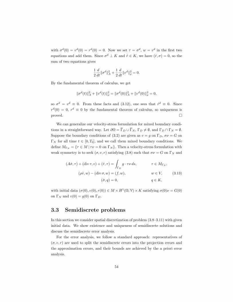
with σd(0) = vd(0) = rd(0) = 0. Now we set τ = σd, w = vd in the first two
equations and add them. Since σd ⊥ K and r ∈ K, we have (r, σ) = 0, so the
sum of two equations gives
1
2
d
dt‖σd‖2A +
1
2
d
dt‖vd‖2ρ = 0.
By the fundamental theorem of calculus, we get
‖σd(t)‖2A + ‖vd(t)‖2ρ = ‖σd(0)‖2A + ‖vd(0)‖2ρ = 0,
so σd = vd ≡ 0. From these facts and (3.12), one sees that rd ≡ 0. Since
rd(0) = 0, rd ≡ 0 by the fundamental theorem of calculus, so uniqueness is
proved.
We can generalize our velocity-stress formulation for mixed boundary condi-
tions in a straightforward way. Let ∂Ω = ΓD ∪ ΓN , ΓD 6= ∅, and ΓD ∩ ΓN = ∅.Suppose the boundary conditions of (3.2) are given as v = g on ΓD, σν = G on
ΓN for all time t ∈ [0, T0], and we call them mixed boundary conditions. We
define MΓN= τ ∈M | τν = 0 on ΓN. Then a velocity-stress formulation with
weak symmetry is to seek (σ, v, r) satisfying (3.8) such that σν = G on ΓN and
(Aσ, τ) + (div τ, v) + (r, τ) =
∫ΓD
g · τν ds, τ ∈MΓN,
(ρv, w)− (div σ,w) = (f, w), w ∈ V, (3.13)
(σ, q) = 0, q ∈ K,
with initial data (σ(0), v(0), r(0)) ∈M ×H1(Ω;V)×K satisfying σ(0)ν = G(0)
on ΓN and v(0) = g(0) on ΓD.
3.3 Semidiscrete problems
In this section we consider spatial discretization of problem (3.8–3.11) with given
initial data. We show existence and uniqueness of semidiscrete solutions and
discuss the semidiscrete error analysis.
For the error analysis, we follow a standard approach: representatives of
(σ, v, r) are used to split the semidiscrete errors into the projection errors and
the approximation errors, and their bounds are achieved by the a priori error
analysis.
54

3.3.1 Existence and uniqueness of semidiscrete solutions
Let Mh × Vh ×Kh be the AFW elements of degree k ≥ 1. For τ ∈Mh, we use
τ ⊥ Kh to denote (τ, q) = 0 for any q ∈ Kh.
Definition 3.2. For initial data (σh(0), vh(0), rh(0)) in Mh×Vh×Kh, a semidis-
crete solution of (3.9–3.11) is
σh ∈ C1([0, T0];Mh), vh ∈ C1([0, T0];Vh), rh ∈ C1([0, T0];Kh),
satisfying the system of equations
(Aσh, τ) + (div τ, vh) + (rh, τ) = 0, τ ∈Mh, (3.14)
(ρvh, w)− (div σh, w) = (f, w), w ∈ Vh, (3.15)
(σh, q) = 0, q ∈ Kh, (3.16)
for all time t ∈ [0, T0] with the given initial data.
Theorem 3.3. For given σh(0) ∈Mh, vh(0) ∈ Vh, and rh(0) ∈ Kh, the system
(3.14–3.16) has a unique solution.
Proof. Let φi, ψi, χi be bases of Mh, Vh, and Kh, respectively. We use
A , B, C , M , D to denote the matrices whose (i, j)-entries are
(Aφj , φi), (div φj , ψi), (φj , χi), (ρψj , ψi), (ψj , ψi),
respectively. We write σh =∑i αiφi, vh =
∑i βiψi, rh =
∑i γiχi, Phf = ζiψi,
and use α, β, γ, ζ to denote the coefficient vectors. Then we may rewrite
(3.14–3.16) in a matrix equation form,A 0 C T
0 M 0
C 0 0
αβγ
=
0 −BT 0
B 0 0
0 0 0
αβγ
+
0
Dζ
0
.
The above matrix equation is a linear system of ordinary differential equations.
Note that the coefficient matrix on the left-hand side is invertible because A
and M are positive definite and C T is injective from the inf-sup condition (A2).
By the standard ODE theory (see [25], p.75), the matrix equation is well-posed
as an initial value problem, so the existence and uniqueness of solutions of
(3.14–3.16) follow.
55

3.3.2 Decomposition of semidiscrete errors
In this section, we state the main result of semidiscrete error analysis and explain
a decomposition of the semidiscrete errors into the projection and the approx-
imation errors. The proof of the main result will be given in the remainder of
this section.
Theorem 3.4. Let (Mh, Vh,Kh) be the AFW elements of degree k ≥ 1 and
let m be an integer such that 1 ≤ m ≤ k. Suppose σ, v, r ∈ W 1,1([0, T0];Hm)
and let (σh, vh, rh) be the semidiscrete solution of (3.14–3.16) with initial data
(σh(0), vh(0), rh(0)) such that
div σh(0) = Ph div σ(0), vh(0) = Phv(0), (3.17)
(Aσh(0), τ) + (rh(0), τ) = 0, for τ ∈Mh, div τ = 0, σh(0) ⊥ Kh, (3.18)
‖σ(0)− σh(0), r(0)− rh(0)‖ ≤ chm‖σ(0), r(0)‖m, (3.19)
for 1 ≤ m ≤ k. Then we have
‖σ − σh, v − vh, r − rh‖L∞L2 ≤ chm‖σ, v, r‖W 1,1Hm ,
where c depends on the compliance tensor A, and the lower and upper bounds
of the mass density ρ0, ρ1, but is independent of h.
We are able to find initial data satisfying (3.17–3.19) when σ(0), v(0) are
given. Since there is u(0) ∈ H1(Ω;V) such that σ(0) = Cε(u(0)) and r(0) =
skw gradu(0), we have (Aσ(0), τ) + (div τ, u(0)) + (r(0), τ) = 0 for τ ∈M . Now
we consider a solution (σh(0), uh(0), rh(0)) of the system,
(Aσh(0), τ) + (div τ, uh(0)) + (rh(0), τ) = 0, τ ∈Mh,
(div σh(0), w) = (div σ(0), w), w ∈ Vh,
(σh(0), q) = 0, q ∈ Kh.
Then (3.18) is obvious from the first and third equations, and (3.19) follows from
the estimate (2.33). The first condition in (3.17) is a consequence of (2.32), so
all conditions in (3.17–3.19) are satisfied.
For our error analysis, we denote the semidiscrete errors, i.e., the difference
of the exact solution (σ, v, r) and the semidiscrete solution (σh, vh, rh), by
eσ = σ − σh, ev = v − vh, er = r − rh.
56

Then, by taking differences of equations (3.9–3.11) and (3.14–3.16), we get
(Aeσ, τ) + (div τ, ev) + (er, τ) = 0, τ ∈Mh, (3.20)
(ρev, w)− (div eσ, w) = 0, w ∈ Vh, (3.21)
(eσ, q) = 0, q ∈ Kh. (3.22)
Recall that Πh is the weakly symmetric elliptic projection in Lemma 2.12 and
Ph, P ′h are the orthogonal L2 projections onto Vh and Kh, respectively. We
decompose the semidiscrete errors (eσ, ev, er) into
eσ = ePσ + ehσ := (σ − σPh ) + (σPh − σh),
ev = ePv + ehv := (v − vPh ) + (vPh − vh), (3.23)
er = ePr + ehr := (r − rPh ) + (rPh − rh),
where σPh := Πhσ, vPh := Phv, and rPh := P ′hr. We call the eP terms the
projection errors and the eh terms the approximation errors, respectively. We
remark that, by (A1) in section 2.4.2 and (2.58),
(div τ, ePv ) := (div τ, v − Phv) = 0, τ ∈Mh,
(div ePσ , w) := (div σ − div Πhσ,w) = 0, w ∈ Vh.(3.24)
By the triangle inequality, Theorem 3.4 will follow from a priori estimates of
the projection errors and the approximation errors, respectively. We state and
prove these estimates in sections 3.3.3 and 3.3.4.
3.3.3 Projection error estimates for the AFW elements
A priori estimates of the L∞L2 norms of the projection errors follow from the
approximation property of Mh × Vh ×Kh.
Theorem 3.5. There exists a constant c > 0 independent of h and t ∈ [0, T0]
such that
‖ePσ ‖L∞L2 ≤ chm‖σ‖L∞Hm , 1 ≤ m ≤ k + 1, (3.25)
‖ePv ‖L∞L2 ≤ chm‖v‖L∞Hm , 0 ≤ m ≤ k, (3.26)
‖ePr ‖L∞L2 ≤ chm‖r‖L∞Hm , 0 ≤ m ≤ k. (3.27)
Furthermore, similar inequalities hold for higher order time derivatives of σ, v,
57

and r, respectively.
Proof. For any t ∈ [0, T0] and 1 ≤ m ≤ k + 1, by (2.57) and (A1), we have
‖ePσ (t)‖ = ‖σ(t)− Πhσ(t)‖ ≤ chm‖σ(t)‖m,
and (3.25) is proved. Similarly, from definitions of ePv and ePr , we have
‖ePv (t)‖ ≤ chm‖v(t)‖m, ‖ePr (t)‖ ≤ chm‖r(t)‖m,
for any t ∈ [0, T0], 0 ≤ m ≤ k. The results for higher order time derivatives
are obtained by applying same argument to higher order time derivatives of
the projection errors because the time derivative and the maps Πh, Ph, Ph are
commutative.
3.3.4 Approximation error estimates for the AFW ele-
ments
We now turn to a priori estimates of the L∞L2 norms of the approximation
errors.
Theorem 3.6. For the approximation error (ehσ, ehv , e
hr ) and 1 ≤ m ≤ k,
‖ehσ, ehv , ehr‖L∞L2 ≤ chm‖σ, v, r‖W 1,1Hm , (3.28)
where c depends on ρ0, ρ1, and A but is independent of h.
Proof. The proof depends on two estimates which we shall prove below: There
exist constants c depending on ρ0, ρ1, and A but is independent of h so that,
‖ehσ, ehv‖L∞L2 ≤ chm(‖σ(0), r(0)‖m + ‖σ, v, r‖L1Hm), (3.29)
‖ehr‖L∞L2 ≤ c‖ehσ, ePσ , ePr ‖L∞L2 , (3.30)
for 1 ≤ m ≤ k. Assuming these estimates are true one can prove Theorem 3.6
easily from Theorem 3.5 because ‖σ(0), r(0)‖m ≤ c‖σ, r‖W 1,1Hm by the Sobolev
embedding.
Now we prove the estimates (3.29–3.30). We first remark that ehσ(0) ⊥ Kh
because σh(0) ⊥ Kh from (3.18) and σPh (0) ⊥ Kh by the definition of σPh (0).
From this fact, and the fact that (ehσ, q) = (ePσ , q) = 0 for all q ∈ Kh, one can
see that ehσ ⊥ Kh by the fundamental theorem of calculus. To show (3.29), we
58
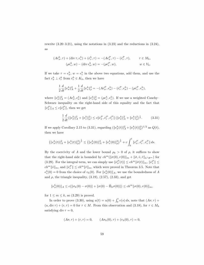
rewrite (3.20–3.21), using the notations in (3.23) and the reductions in (3.24),
as
(Aehσ, τ) + (div τ, ehv ) + (ehr , τ) = −(AePσ , τ)− (ePr , τ), τ ∈Mh,
(ρehv , w)− (div ehσ, w) = −(ρePv , w), w ∈ Vh.
If we take τ = ehσ, w = ehv in the above two equations, add them, and use the
fact ehσ ⊥ ehr from ehr ∈ Kh, then we have
1
2
d
dt‖ehσ‖2A +
1
2
d
dt‖ehv‖2ρ = −(AePσ , e
hσ)− (ePr , e
hσ)− (ρePv , e
hv ),
where ‖ehσ‖2A = (Aehσ, ehσ) and ‖ehv‖2ρ = (ρehv , e
hv ). If we use a weighted Cauchy–
Schwarz inequality on the right-hand side of this equality and the fact that
‖ePσ ‖A ≤ c‖ePσ ‖, then we get
1
2
d
dt(‖ehσ‖2A + ‖ehv‖2ρ) ≤ c‖ePσ , ePr , ePv ‖ (‖ehσ‖2A + ‖ehv‖2ρ)
12 . (3.31)
If we apply Corollary 2.15 to (3.31), regarding (‖ehσ(t)‖2A+‖ehv (t)‖2ρ)1/2 as Q(t),
then we have
(‖ehσ(t)‖2A + ‖ehv (t)‖2ρ
) 12 ≤
(‖ehσ(0)‖2A + ‖ehv (0)‖2ρ
) 12 + c
∫ t
0
‖ePσ , ePr , ePv ‖ ds.
By the coercivity of A and the lower bound ρ0 > 0 of ρ, it suffices to show
that the right-hand side is bounded by chm(‖σ(0), r(0)‖m + ‖σ, v, r‖L1Hm) for
(3.29). For the integral term, we can simply use ‖ePσ (t)‖ ≤ chm‖σ(t)‖m, ‖ePv ‖ ≤chm‖v‖m, and ‖ePr ‖ ≤ chm‖r‖m, which were proved in Theorem 3.5. Note that
ehv (0) = 0 from the choice of vh(0). For ‖ehσ(0)‖A, we use the boundedness of A
and ρ, the triangle inequality, (3.19), (2.57), (2.33), and get
‖ehσ(0)‖A ≤ c(‖σh(0)− σ(0)‖+ ‖σ(0)− Πhσ(0)‖) ≤ chm‖σ(0), r(0)‖m,
for 1 ≤ m ≤ k, so (3.29) is proved.
In order to prove (3.30), using u(t) = u(0) +∫ t
0v(s) ds, note that (Aσ, τ) +
(u,div τ) + (r, τ) = 0 for τ ∈M . From this observation and (3.18), for τ ∈Mh
satisfying div τ = 0,
(Aσ, τ) + (r, τ) = 0, (Aσh(0), τ) + (rh(0), τ) = 0,
59

so (Aeσ(0), τ) + (er(0), τ) = 0. If we consider (3.20) for τ ∈ Mh satisfying
div τ = 0, and the fundamental theorem of calculus, then we have
(Aeσ(t), τ) + (er(t), τ) = 0, τ ∈Mh, div τ = 0,
for all t ∈ [0, T0]. This is equivalent to
(ehr (t), τ) = −(A(ehσ(t) + ePσ (t)), τ) + (ePr (t), τ), τ ∈Mh, div τ = 0.
By (A2) in section 2.4.2, we can choose τ ∈ Mh such that div τ = 0, (τ, q) =
‖ehr (t)‖2, and ‖τ‖ ≤ c‖ehr (t)‖ for each t ∈ [0, T0]. If we take such τ in the above
equation, then we get ‖ehr (t)‖ ≤ c‖ehσ(t), ePσ (t), ePr (t)‖ by the Cauchy–Schwarz
inequality, so (3.30) follows.
3.4 Full discretization
In this section, we use the Crank–Nicolson scheme for full discretization and
prove a priori error estimates of fully discrete solutions for the AFW elements.
We use ∆t > 0 to denote the time step interval. For given T0 > 0, we assume
that ∆t, N , and tj for 0 ≤ j ≤ N are defined as in section 2.1.
The fully discrete solution of (σ, v, r) at time tj will be denoted by (Σj , V j , Rj).
Let the initial data (Σ0, V 0, R0) be given. In the Crank–Nicolson scheme, using
notations in (2.3), the sequence (Σj+1, V j+1, Rj+1) for 1 ≤ j ≤ N is defined
inductively by(A∂tΣ
j+ 12 , τ)
+ (V j+12 ,div τ) + (∂tR
j+ 12 , τ) = 0, (3.32)(
ρ∂tVj+ 1
2 , w)− (div Σj+
12 , w) = (f j+
12 , w), (3.33)
(∂tΣj+ 1
2 , q) = 0, (3.34)
for (τ, w, q) ∈Mh × Vh ×Kh.
Theorem 3.7. Let Mh × Vh ×Kh be the AFW elements of degree k ≥ 1. For
given initial data (Σ0, V 0, R0) ∈ Mh × Vh × Kh, the sequence of fully discrete
solutions (Σj , V j , Rj) for 1 ≤ j ≤ N is well-defined by (3.32–3.34). Suppose
σ, v, r ∈W 1,1([0, T0];Hm) ∩W 3,1([0, T0];L2), (3.35)
and the initial data (Σ0, V 0, R0) satisfies the conditions (3.17–3.19). Then the
60

fully discrete solution (Σj , V j , Rj) satisfies
‖σj − Σj , vj − V j , rj −Rj‖ ≤ c(∆t2 + hm)‖σ, v, r‖W 1,1Hm∩W 3,1L2 , (3.36)
for c > 0 which depends on A, ρ0, ρ1, but is independent of h and ∆t.
The proof of this theorem will be given in the rest of this section.
3.4.1 Well-definedness
First of all, we show the fully discrete solution is well-defined. We need to
check that (Σj+1, V j+1, Rj+1) is uniquely determined as a solution of the linear
system (3.32–3.34) when Σj , V j , Rj , f j , f j+1 are given. Rewriting (3.32–3.34),
we have
(AΣj+1, τ
)+
∆t
2(V j+1,div τ) + (Rj+1, τ)
= (AΣj , τ)− ∆t
2(V j ,div τ) + (Rj , τ),
(ρV j+1, w)− ∆t
2(div Σj+1, w) = (ρV j , w) +
∆t
2(div Σj , w) + ∆t(f j+
12 , w),
(Σj+1, q) = (Σj , q),
for (τ, w, q) ∈Mh×Vh×Kh. Note that the above is a system of linear equations
with same number of equations and unknowns. In order to show that its solution
(Σj+1, V j+1, Rj+1) exists uniquely, it suffices to show that Σj+1 = V j+1 =
Rj+1 = 0 if all right-hand sides vanish. Suppose the right-hand sides vanish. If
we take τ = Σj+1, w = V j+1, q = −Rj+1 in the above equations and add them,
then we have (AΣj+1,Σj+1)+(ρV j+1, V j+1) = 0 which yields Σj+1 = V j+1 = 0.
By Corollary 2.4, there is τ ∈ Mh so that (Rj+1, τ) = (Rj+1, Rj+1). If we
take such τ in the first equation of the system, we obtain Rj+1 = 0 since
Σj+1 = V j+1 = 0. Hence the full discretization is well-defined.
61

3.4.2 Convergence
We now turn to the proof of the a priori estimate (3.36). Let us denote the
errors (σj − Σj , vj − V j , rj −Rj) by
Ejσ := σj − Σj = (σj − σP,jh ) + (σP,jh − Σj) =: eP,jσ + θjσ, (3.37)
Ejv := vj − V j = (vj − vP,jh ) + (vP,jh − V j) =: eP,jv + θjv, (3.38)
Ejr := rj −Rj = (rj − rP,jh ) + (rP,jh −Rj) =: eP,jr + θjr. (3.39)
In Theorem 3.5 of semidiscrete error analysis, we already obtained error bounds
of the projection errors (ePσ , ePv , e
Pr ). Thus we only need to consider a priori
estimates of (θjσ, θjv, θ
jr) for Theorem 3.7. Here is a precise statement of our
claim.
Theorem 3.8. Suppose the assumptions of Theorem 3.7 hold and θiσ, θiv, θir
are defined as in (3.37–3.39). Then there exists a constant c > 0 such that
‖θiσ, θiv, θir‖ ≤ c(∆t2 + hm)‖σ, v, r‖W 1,1Hm∩W 3,1L2 , (3.40)
for 1 ≤ i ≤ N , 1 ≤ m ≤ k, where the constant c depends on A, ρ0, ρ1 but is
independent of h and ∆t.
Proof. In order to show (3.40), consider the arithmetic mean of equations (3.9–
3.10) at t = tj and t = tj+1, which are
(Aˆσj+12 , τ) + (div τ, vj+
12 ) + (ˆrj+
12 , τ) = 0, τ ∈Mh,
(ρˆvj+12 , w)− (div σj+
12 , w) = (f j+
12 , w), w ∈ Vh.
We subtract (3.32–3.33) from the above two equations and consider the differ-
ence of equations. If we rewrite the difference of equations using (Eσ, Ev, Er)
defined in (3.37–3.39),
(A(ˆσj+12 − ∂tΣj+
12 ), τ) + (div τ, E
j+ 12
v ) + (ˆrj+12 − ∂tRj+
12 , τ) = 0,
(ρˆvj+12 − ρ∂tV j+
12 , w)− (div E
j+ 12
σ , w) = 0,
for (τ, w) ∈Mh×Vh. If we do some algebraic manipulations on those equations
62

regarding equalities
ˆσj+12 − ∂tΣj+
12 = ˆσj+
12 − ∂tσj+
12 + ∂tE
j+ 12
σ ,
ˆrj+12 − ∂tRj+
12 = ˆrj+
12 − ∂trj+
12 + ∂tE
j+ 12
r ,
ˆvj+12 − ∂tV j+
12 = ˆvj+
12 − ∂tvj+
12 + ∂tE
j+ 12
v ,
then one can have
(A∂tEj+ 1
2σ , τ) + (div τ, E
j+ 12
v ) + (∂tEj+ 1
2r , τ)
= (A(∂tσj+ 1
2 − ˆσj+12 ), τ) + (∂tr
j+ 12 − ˆrj+
12 , τ),
(3.41)
(ρ∂tEj+ 1
2v , w)− (div E
j+ 12
σ , w) = (ρ∂tvj+ 1
2 − ρˆvj+12 , w). (3.42)
Considering the decomposition of errors in (3.37–3.39) and using the reductions
from (3.24), we have
(A∂tθj+ 1
2σ , τ) + (div τ, θ
j+ 12
v ) + (∂tθj+ 1
2r , τ)
= (A(ωj+ 1
21 + ω
j+ 12
2 ) + ωj+ 1
23 + ω
j+ 12
4 , τ),(3.43)
(ρ∂tθj+ 1
2v , w)− (div θ
j+ 12
σ , w) = (ωj+ 1
25 + ω
j+ 12
6 , w), (3.44)
where
ωj+ 1
21 = ∂tσ
j+ 12 − ˆσj+
12 , ω
j+ 12
2 = −∂teP,j+ 1
2σ , ω
j+ 12
3 = ∂trj+ 1
2 − ˆrj+12 ,
ωj+ 1
24 = −∂te
P,j+ 12
r , ωj+ 1
25 = ρ(∂tv
j+ 12 − ˆvj+
12 ), ω
j+ 12
6 = −ρ∂teP,j+ 1
2v .
(3.45)
Letting τ = θj+1/2σ , w = θ
j+1/2v in (3.43) and (3.44), and adding those equations,
(‖θj+1σ ‖2A + ‖θj+1
v ‖2ρ)− (‖θjσ‖2A + ‖θjv‖2ρ) (3.46)
= 2∆t(A(ωj+ 1
21 + ω
j+ 12
2 ) + ωj+ 1
23 + ω
j+ 12
4 , θj+ 1
2σ ) + 2∆t(ω
j+ 12
5 + ωj+ 1
26 , θ
j+ 12
v ).
If we divide both sides by (‖θj+1σ ‖2A + ‖θj+1
v ‖2ρ)1/2 + (‖θjσ‖2A + ‖θjv‖2ρ)1/2 and
apply a weighted Cauchy–Schwarz inequality, then we get
(‖θj+1σ ‖2A + ‖θj+1
v ‖2ρ)12 ≤ (‖θjσ‖2A + ‖θjv‖2ρ)
12 + c∆t
6∑l=1
‖ωj+12
l ‖, (3.47)
63

for each 0 ≤ j ≤ N − 1, with c independent of h, ∆t, and j. By using (3.47)
inductively, we have
(‖θiσ‖2A + ‖θiv‖2ρ)12 ≤ (‖θ0
σ‖2A + ‖θ0v‖2ρ)
12 + c∆t
i−1∑j=0
6∑l=1
‖ωj+12
l ‖. (3.48)
Since A is coercive and 0 < ρ0 ≤ ρ for a constant ρ0, there exists c > 0 depending
only on A and ρ0 such that
‖θiσ‖+ ‖θiv‖ ≤ c(‖θiσ‖2A + ‖θiv‖2ρ)12 . (3.49)
We can see that (‖θ0σ‖2A + ‖θ0
v‖2ρ)12 = ‖θ0
σ‖A ≤ chm‖σ(0), r(0)‖m holds by an
argument similar to that of semidiscrete error analysis from the fact θ0v = 0,
the assumption (3.19) of (Σ0, V 0, R0), and the triangle inequality. Hence, if we
show
c∆t
i−1∑j=0
6∑l=1
‖ωj+12
l ‖ ≤ c(∆t2 + hm), 1 ≤ m ≤ k, (3.50)
then the estimate (3.40) for ‖θiσ‖+ ‖θiv‖ is proved by (3.48) and (3.49).
In order to show the above inequality, we recall Taylor expansions for g ∈C4([−a, a]),
|g(a)− g(−a)− 2ag′(0)| ≤ ca2‖g′′′‖L1(−a,a), (3.51)
|g(a) + g(−a)− 2g(0)| ≤ ca‖g′′‖L1(−a,a), (3.52)
|g(a)− g(−a)− a(g′(a) + g′(−a))| ≤ ca2‖g′′′‖L1(−a,a), (3.53)
|2g(a)− 4g(0) + 2g(−a)− a(g′(a)− g′(−a))| ≤ ca3‖g(4)‖L1(−a,a), (3.54)
where g(4) denotes the fourth derivative of g.
From the definitions of ωj+1/2l , l = 1, 3, 5 in (3.45), we can use (3.53) by
64

substituting a by ∆t/2, 0 by tj , and g by σ, v, r. Then we have
∆t‖ωj+12
1 ‖ =1
2‖2σj+1 − 2σj −∆tσj+1 −∆tσj‖ ≤ c∆t2
∫ tj+1
tj
‖...σ‖ ds, (3.55)
∆t‖ωj+12
3 ‖ =1
2‖2rj+1 − 2rj −∆trj+1 −∆trj‖ ≤ c∆t2
∫ tj+1
tj
‖...r ‖ ds, (3.56)
∆t‖ωj+12
5 ‖ =1
2‖ρ(2vj+1 − 2vj −∆tvj+1 −∆tvj)‖ ≤ c∆t2
∫ tj+1
tj
‖...v ‖ ds.
(3.57)
By the definitions of ωj+1/2l , l = 2, 4, 6 in (3.45), and Theorem 3.5, one can see
∆t‖ωj+12
2 ‖ = ∆t‖∂teP,j+ 1
2σ ‖ =
∥∥∥∥∥∫ tj+1
tj
ePσ ds
∥∥∥∥∥ ≤ chm∫ tj+1
tj
‖σ‖m ds, (3.58)
∆t‖ωj+12
4 ‖ = ∆t‖∂teP,j+ 1
2r ‖ =
∥∥∥∥∥∫ tj+1
tj
ePr ds
∥∥∥∥∥ ≤ chm∫ tj+1
tj
‖r‖m ds, (3.59)
∆t‖ωj+12
6 ‖ = ∆t‖ρ∂teP,j+ 1
2v ‖ =
∥∥∥∥∥∫ tj+1
tj
ρePv ds
∥∥∥∥∥ ≤ chm∫ tj+1
tj
‖v‖m ds, (3.60)
for 1 ≤ m ≤ k. The estimate (3.50) is obtained by combining (3.55–3.60) and
as we remarked before, the estimate (3.40) is proved for ‖θiσ, θiv‖.To complete the proof of (3.40), we estimate ‖θir‖ following the outline of
semidiscrete analysis. We first note that (Aσj , τ) + (rj , τ) = 0 for 0 ≤ j ≤ N ,
for all τ ∈Mh such that div τ = 0. From the condition (3.18) of initial data, we
have (AΣ0, τ) + (R0, τ) = 0 and combining this equality with (3.32), we get
(AΣj , τ) + (Rj , τ) = 0, τ ∈Mh, div τ = 0, 0 ≤ j ≤ N.
Therefore we have an error equation (AEjσ, τ) + (Ejr , τ) = 0 for τ ∈ Mh such
that div τ = 0, which is equivalent to
(θjr, τ) = −(A(θjσ + eP,jσ ), τ)− (eP,jr , τ), τ ∈Mh, div τ = 0, 0 ≤ j ≤ N.
If we take τ ∈ Mh such that div τ = 0, (τ, q) = ‖θjr‖2, and ‖τ‖ ≤ c‖θjr‖ by
(A2), then we obtain
‖θjr‖ ≤ c‖θjσ, eP,jσ , eP,jr ‖ ≤ c(‖θjσ‖+ hm‖σ, r‖L∞Hm).
65

Combining this with the estimate of ‖θjσ‖, then the estimate (3.40) for ‖θjr‖ is
proved.
In some applications, we need to compute numerical solutions of the displace-
ment. Let U0 ∈ Vh be an approximation of initial displacement u(0). Then we
can compute a numerical displacement U i from V j, using the trapezoidal rule,
as
U i = U0 + ∆t
i∑j=1
V j + V j−1
2= U0 + ∆t
i∑j=1
V j+12 . (3.61)
Corollary 3.9 (Numerical solutions of displacement). Let U0 ∈ Vh be an
approximation of initial displacement u(0) with ‖u(0) − U0‖ ≤ chm‖u(0)‖m,
1 ≤ m ≤ k, and U i be defined by (3.61). Then, for 0 ≤ i ≤ N , 1 ≤ m ≤ k,
‖ui − U i‖ ≤ c(hm + ∆t2)(‖u(0)‖m + ‖σ, v, r‖W 1,1Hm∩W 3,1L2).
Proof. Noting that ui = u0 +∫ ti
0v ds and using the triangle inequality,
‖ui − U i‖ ≤ ‖u(0)− U0‖+
i∑j=1
∥∥∥∥∥∫ tj
tj−1
v ds−∆tV j+12
∥∥∥∥∥ . (3.62)
Recall an estimate in the trapezoidal rule, which is∣∣∣∣∫ a
−ag(s) ds− a(g(a) + g(−a))
∣∣∣∣ ≤ ca3‖g′′‖L∞(−a,a).
Combining the triangle inequality, the above estimate, and ‖vj −V j‖ ≤ c(hm +
∆t2) from Theorem 3.7 yields∥∥∥∥∥∫ tj
tj−1
v ds−∆tV j+12
∥∥∥∥∥ ≤∥∥∥∥∥∫ tj
tj−1
v ds−∆tvj+12
∥∥∥∥∥+ ∆t‖vj+ 12 − V j+ 1
2 ‖
≤ c∆t3‖v‖L∞L2 + c(hm + ∆t2)∆t. (3.63)
The conclusion follows from the assumption of U0, (3.62), and (3.63).
66

3.5 Error analysis for the GG elements
In this section we discuss the error analysis for the GG elements. We shall show
that we can obtain better error bounds of σ and r for the GG elements than for
the AFW elements when the degree k of elements are same. We also show that
a postprocessing is eligible for the GG elements to obtain a better numerical
solution of u.
3.5.1 A priori error estimates
Since many steps of the error analysis for the GG elements are similar to the
one for the AFW elements, we do not repeat all details but focus on the steps
that should be modified. Before we state a main result, we define ‖ρ‖W 1,∞h
as
‖ρ‖W 1,∞h
= ‖ρ‖L∞ + ‖ gradh ρ‖L∞ , (3.64)
where gradh is the piecewise gradient operator adapted to the triangulation Th.
Theorem 3.10. Let (Mh, Vh,Kh) be the GG elements of degree k ≥ 1, m be
an integer for which 1 ≤ m ≤ k + 1, and m′ = m− δm,k+1 where δm,k+1 is the
Kronecker delta. Suppose ‖ρ‖W 1,∞h
<∞ and
σ, r ∈W 1,1([0, T0];Hm) ∩W 3,1([0, T0];L2),
v ∈W 1,1([0, T0];Hm′) ∩W 3,1([0, T0];L2).(3.65)
Assume the initial data satisfy (3.17–3.19) for 1 ≤ m ≤ k + 1. Then the fully
discrete solution (Σj , V j , Rj) in (3.32–3.34) is well-defined and for all 0 ≤ j ≤N ,
‖σj − Σj‖+ ‖Phvj − V j‖+ ‖rj −Rj‖ ≤ c(∆t2 + hm),
‖vj − V j‖ ≤ c(∆t2 + hm′),
(3.66)
where c depends on the quantities ‖σ, r‖W 1,1Hm∩W 3,1L2 , ‖v‖W 1,1Hm′∩W 3,1L2 , A,
ρ0, and ‖ρ‖W 1,∞h
but is independent of h and ∆t.
In comparison with Theorem 3.7, if k is same, the above theorem gives better
accuracy of the errors of σ and r. In particular, we will show later that we can
use the estimate of ‖Phvj − V j‖ for a postprocessing for the numerical solution
of u.
67
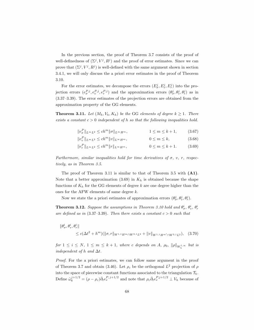
In the previous section, the proof of Theorem 3.7 consists of the proof of
well-definedness of (Σj , V j , Rj) and the proof of error estimates. Since we can
prove that (Σj , V j , Rj) is well-defined with the same argument shown in section
3.4.1, we will only discuss the a priori error estimates in the proof of Theorem
3.10.
For the error estimates, we decompose the errors (Ejσ, Ejv, E
jr) into the pro-
jection errors (eP,jσ , eP,jv , eP,jr ) and the approximation errors (θjσ, θjv, θ
jr) as in
(3.37–3.39). The error estimates of the projection errors are obtained from the
approximation property of the GG elements.
Theorem 3.11. Let (Mh, Vh,Kh) be the GG elements of degree k ≥ 1. There
exists a constant c > 0 independent of h so that the following inequalities hold.
‖ePσ ‖L∞L2 ≤ chm‖σ‖L∞Hm , 1 ≤ m ≤ k + 1, (3.67)
‖ePv ‖L∞L2 ≤ chm‖v‖L∞Hm , 0 ≤ m ≤ k, (3.68)
‖ePr ‖L∞L2 ≤ chm‖r‖L∞Hm , 0 ≤ m ≤ k + 1. (3.69)
Furthermore, similar inequalities hold for time derivatives of σ, v, r, respec-
tively, as in Theorem 3.5.
The proof of Theorem 3.11 is similar to that of Theorem 3.5 with (A1).
Note that a better approximation (3.69) in Kh is obtained because the shape
functions of Kh for the GG elements of degree k are one degree higher than the
ones for the AFW elements of same degree k.
Now we state the a priori estimates of approximation errors (θjσ, θjv, θ
jr).
Theorem 3.12. Suppose the assumptions in Theorem 3.10 hold and θiσ, θiv, θir
are defined as in (3.37–3.39). Then there exists a constant c > 0 such that
‖θiσ, θiv, θir‖
≤ c(∆t2 + hm)(‖σ, r‖W 1,1Hm∩W 3,1L2 + ‖v‖W 1,1Hm′∩W 3,1L2), (3.70)
for 1 ≤ i ≤ N , 1 ≤ m ≤ k + 1, where c depends on A, ρ0, ‖ρ‖W 1,∞h
but is
independent of h and ∆t.
Proof. For the a priori estimates, we can follow same argument in the proof
of Theorem 3.7 and obtain (3.46). Let ρc be the orthogonal L2 projection of ρ
into the space of piecewise constant functions associated to the triangulation Th.
Define ωj+1/26 = (ρ− ρc)∂teP, j+1/2
v and note that ρc∂teP,j+1/2v ⊥ Vh because of
68

eP,jv , eP,j+1v ⊥ Vh and the facts that ρc is a piecewise constant function and Vh
is a space of piecewise polynomials without any interelement continuity. From
the orthogonality ρc∂teP,j+1/2v ⊥ Vh, one can see that
(ωj+ 1
26 , θ
j+ 12
v ) = (ρ∂teP,j+ 1
2v , θ
j+ 12
v ) = ((ρ− ρc)∂teP,j+ 1
2v , θ
j+ 12
v ) = (ωj+ 1
26 , θ
j+ 12
v ).
Therefore, by replacing ωj+1/26 by ω
j+1/26 and repeating the steps in (3.46–3.48),
we have an inequality analogous to (3.48),
(‖θj+1σ ‖2A + ‖θj+1
v ‖2ρ)12 ≤ (‖θ0
σ‖2A + ‖θ0v‖2ρ)
12 + c∆t
(5∑l=1
‖ωj+12
l ‖+ ‖ωj+12
6 ‖
).
The first term can be bounded by chm‖σ(0), r(0)‖m by (3.19) as we have seen
before. To prove (3.70) for ‖θiσ‖+ ‖θiv‖, we only need to show
c∆t
i−1∑j=0
(5∑l=1
‖ωj+12
l ‖+ ‖ωj+12
6 ‖
)≤ c(∆t2 + hm), 1 ≤ m ≤ k + 1.
For the estimates of ωj+1/2l , l = 1, 3, 5, we use (3.55–3.57). For the estimates
of ωj+1/22 and ω
j+1/24 , we use (3.58) and (3.59), respectively and note that the
integer m ranges 1 ≤ m ≤ k + 1 for the GG elements. For ωj+1/26 , we use
∆t‖ωj+12
6 ‖ = ∆t‖(ρ− ρc)∂tvP,j‖ =
∥∥∥∥∥∫ tj+1
tj
(ρ− ρc)(vPh − v) ds
∥∥∥∥∥≤ chm+1‖ρ‖W 1,∞
h
∫ tj+1
tj
‖v‖m ds, 1 ≤ m ≤ k,
and the proof of (3.70) for ‖θiσ‖+ ‖θiv‖ is completed.
For the proof of (3.70) we omit details because the proof is same as that of
‖θir‖ estimate in Theorem 3.7.
The proof of Theorem 3.10 follows from the above theorem and Theorem
3.11. Note that Phvj − V j = θjv and the ‖Phvj − V j‖ estimate in (3.66) is a
consequence of (3.70). The other estimates in (3.66) are easily obtained from
the estimates (3.67–3.69), (3.70), and the triangle inequality.
69

3.5.2 Postprocessing
We show that a postprocessing is eligible for the GG elements. For simplicity, we
only consider the numerical solution of displacement u defined in Corollary 3.9.
We shall show that a better numerical solution of u is obtained by a relatively
simple computation.
For Vh in the GG elements, let V ∗h be the space of (possibly discontinuous)
piecewise polynomials adapted to Th of one degree higher than Vh, and Vh be
the orthogonal complement of Vh in V ∗h . The orthogonal L2 projections onto
V ∗h and Vh are denoted by P ∗h and Ph, respectively. We claim the following
postprocessing result.
Theorem 3.13. Suppose that the assumptions of Theorem 3.10 holds with
m = k + 1 and (Σi, V i, Ri) is the fully discrete solution. Suppose also that
‖v‖W 1,1Hk+1 is finite. Let U i be the numerical solution of displacement in Corol-
lary 3.9 with the assumption ‖Phu(0)− U0‖ ≤ chk+1. We define U∗,i ∈ V ∗h by
(gradh U∗,i, gradh w) = (AΣi +Ri, gradh w), w ∈ Vh, (3.71)
(U∗,i, w) = (U i, w), w ∈ Vh, (3.72)
for each 0 ≤ i ≤ N where gradh is the piecewise gradient operator adapted to the
triangulation Th. Then U∗,i is well-defined and there exists c > 0 independent
of h and ∆t such that
‖ui − U∗,i‖ ≤ c(∆t2 + hk+1)‖σ, v, r‖W 1,1Hk+1∩W 3,1L2 , (3.73)
where c depends on A, ρ0, ‖ρ‖W 1,∞h
.
Proof. We can show that U∗,i is well-defined with the same argument we used in
(2.48), so we omit details. Note that PhU∗,i = U i and let U i := U∗,i−U i ∈ Vh.
To prove (3.73), by the triangle inequality and the Bramble–Hilbert lemma,
it suffices to show ‖P ∗hui−U∗,i‖ ≤ c(∆t2+hk+1). To show this reduced estimate,
consider
P ∗hui − U∗,i = (Phu
i − U i) + (Phui − U i) ∈ Vh ⊕ Vh.
We first show that
‖Phui − U i‖ ≤ c(∆t2 + hk+1)‖σ, v, r‖W 1,1Hk+1∩W 3,1L2 . (3.74)
70

From the definition of U i,
‖Phui − U i‖ =
∥∥∥∥∥Phu(0)− U0 +
∫ ti
0
Phv ds−∆t
i−1∑j=0
V j+12
∥∥∥∥∥≤ ‖Phu(0)− U0‖+
i−1∑j=0
∥∥∥∥∥∫ tj+1
tj
Phv ds−∆tPhvj+ 1
2
∥∥∥∥∥+ ∆t
i−1∑j=0
‖Phvj+12 − V j+ 1
2 ‖
≤ chk+1 + ∆t2‖Phv‖L∞L2 + c(∆t2 + hk+1),
where the last inequality is due to the assumption of U0, the error bound of
trapezoidal rule, and the ‖Phvj − V j‖ estimate in (3.66). Thus the desired
estimate (3.74) is proved.
Now we turn to the estimation of ‖Phui− U i‖. Since gradui = Aσi + ri, we
have (gradh ui, gradh w) = (Aσi + ri, gradh w) for w ∈ Vh. By subtracting the
equation (3.71) from this equation, we get, for w ∈ Vh,
(gradh(ui − U∗,i), gradh w) = (A(σi − Σi) + ri −Ri, gradh w). (3.75)
Regarding equalities,
ui − U∗,i = (ui − P ∗hui) + (P ∗hui − U∗,i)
= (ui − P ∗hui) + (Phui − U i) + (Phu
i − U i),
and by replacing ui − U∗,i in (3.75), a direct computation gives
(gradh(Phui − U i), gradh w)
= −(gradh(ui − P ∗hui), gradh w)− (gradh(Phui − U i), gradh w)
+ (A(σi − Σi) + ri −Ri, gradh w).
Taking w = Phui − U i in this equation, we have
‖ gradh(Phui − U i)‖
≤ c(‖ gradh(ui − P ∗hui)‖+ ‖ gradh(Phui − U i)‖
+ ‖A(σi − Σi) + ri −Ri‖). (3.76)
71

By applying (2.53) to Phui− U i, we have ‖Phui− U i‖ ≤ ch‖ gradh(Phu
i− U i)‖.From this inequality, by using the inequality that we multiply h to (3.76), we
get
‖Phui − U i‖ ≤ ch(‖ gradh(ui − P ∗hui)‖+ ‖ gradh(Phui − U i)‖
+ ‖A(σi − Σi) + ri −Ri‖)
≤ ch‖ gradh(ui − P ∗hui)‖+ c‖Phui − U i‖
+ ch‖A(σi − Σi) + ri −Ri‖,
where the second term on the right-hand side of last inequality is due to (2.52).
Now we only need to prove that the three quantities on the right-hand side of
the above inequality are bounded by c(∆t2 + hk+1).
For the first term, one can see h‖ gradh(ui−P ∗hui)‖ ≤ chk+1‖ui‖k+1, by the
Bramble–Hilbert lemma. For the second, we use (3.74). For the third, we use
the triangle inequality and (3.66). The proof is completed.
Remark 3.14. This postprocessing does not need postprocessing of all the pre-
vious time steps.
3.6 Robustness for nearly incompressible mate-
rials
In this section, we assume that an elastic medium is homogeneous isotropic,
i.e., the compliance tensor A has the form (2.7) with the Lame coefficients µ
and λ which are constants. We also assume that the boundary conditions are
the homogeneous displacement boundary conditions. In nearly incompressible
elastic materials, λ is very large, and, in the incompressible limit, λ = +∞.
Many standard discretization of elasticity suffer from locking, which means that
the errors, while they decay with the mesh size, grow as λ increases. A robust
or locking-free method is one in which the error estimates hold uniformly as
λ→ +∞. As we have seen in Theorem 2.5, stable mixed methods for stationary
elasticity problems are typically locking-free (see [8, 19]). In this section, we
will show that the locking-free advantage of mixed methods still holds in our
numerical schemes for linear elastodynamics.
Theorem 3.15. Let Mh × Vh ×Kh be the AFW elements of degree k ≥ 1 and
assume that A have the form of (2.7) with constants µ and λ. We assume that
72
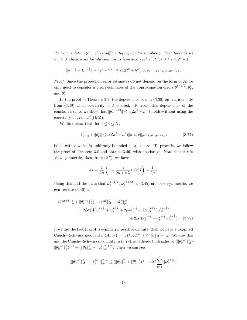
the exact solution (σ, v, r) is sufficiently regular for simplicity. Then there exists
a c > 0 which is uniformly bounded as λ→ +∞ such that for 0 ≤ i ≤ N − 1,
‖σi− 12 − Σi−
12 ‖+ ‖vi − V i‖ ≤ c(∆t2 + hk)‖σ, v, r‖W 2,1Hk∩W 4,1L2 .
Proof. Since the projection error estimates do not depend on the form of A, we
only need to consider a priori estimates of the approximation errors θi+1/2σ , θiv,
and θir.
In the proof of Theorem 3.7, the dependence of c in (3.36) on λ arises only
from (3.49) when coercivity of A is used. To avoid this dependence of the
constant c on λ, we show that ‖θj+1/2σ ‖ ≤ c(∆t2 + hm) holds without using the
coercivity of A on L2(Ω;M).
We first show that, for 1 ≤ i ≤ N ,
‖θiσ‖A + ‖θiv‖ ≤ c(∆t2 + hk)‖σ, v, r‖W 2,1Hk∩W 4,1L2 , (3.77)
holds with c which is uniformly bounded as λ → +∞. To prove it, we follow
the proof of Theorem 3.8 and obtain (3.46) with no change. Note that if τ is
skew-symmetric, then, from (2.7), we have
Aτ =1
2µ
(τ − λ
2µ+ nλtr(τ)I
)=
1
2µτ.
Using this and the facts that ωj+1/23 , ω
j+1/24 in (3.45) are skew-symmetric, we
can rewrite (3.46) as
(‖θj+1σ ‖2A + ‖θj+1
v ‖2ρ)− (‖θjσ‖2A + ‖θjv‖2ρ)
= 2∆t(A(ωj+ 1
21 + ω
j+ 12
2 + 2µωj+ 1
23 + 2µω
j+ 12
4 ), θj+ 1
2σ )
+ 2∆t(ωj+ 1
25 + ω
j+ 12
6 , θj+ 1
2v ). (3.78)
If we use the fact that A is symmetric positive definite, then we have a weighted
Cauchy–Schwarz inequality, (Aσ, τ) = (A12σ,A
12 τ) ≤ ‖σ‖A‖τ‖A. We use this
and the Cauchy–Schwarz inequality to (3.78), and divide both sides by (‖θj+1σ ‖2A+
‖θj+1v ‖2ρ)1/2 + (‖θjσ‖2A + ‖θjv‖2ρ)1/2. Then we can see
(‖θj+1σ ‖2A + ‖θj+1
v ‖2ρ)12 ≤ (‖θjσ‖2A + ‖θjv‖2ρ)
12 + c∆t
6∑l=1
‖ωj+12
l ‖.
73

By applying the estimates (3.55–3.56), (3.58–3.59), we obtain (3.77).
As a consequence of (3.77), it is easy to see that the error estimate for the
error of v holds with a constant c which is uniformly bounded as λ→ +∞. Now
we consider the estimate for the error of σ.
From the form of A in (2.7), we have
(Aτ, I) =1
2µ+ nλ
∫Ω
tr(τ) dx. (3.79)
We first note that (Aσ, I) = 0 by taking τ = I in (3.9). Moreover, (Aσ, I) = 0
because (Aσ, I) = (ε(u), I) = (gradu, I) = (u,div I) = 0. By using these facts,
we have (A∂tEj+1/2σ , I) = 0 if we take τ = I in (3.41) because div I = 0 and
r, r are skew-symmetric. From the assumption (3.18), (AE0σ, I) = 0, whence
(AEjσ, I) = 0 for all 0 ≤ j ≤ N . Furthermore, (AeP,jσ , I) = (eP,jσ , AI) = 0 from
the definitions of ePσ and Πh in (2.57), and the facts that divAI = 0, AI ⊥ Kh.
Thus we have (Aθjσ, I) = 0 for 0 ≤ j ≤ N .
If we recall AI = (2µ + nλ)−1I, then (θjσ, AI) = 0 implies∫
Ωtr(θjσ) dx = 0
for λ < +∞ and (2.43) can be applied to θjσ. By Lemma 2.6 and Lemma 2.7,
‖θj+12
σ ‖2 ≤ c(‖θj+12
σ ‖2A + ‖ div θj+ 1
2σ ‖2−1). (3.80)
Note that ‖θj+12
σ ‖2A can be estimated by (3.77) with a uniform constant c not
growing as λ → +∞. To handle ‖ div θj+1/2σ ‖2−1, we take w = div θ
j+1/2σ in
(3.44) and get ‖ div θj+1/2σ ‖ ≤ c(‖∂tθj+1/2
v ‖ + ‖ωj+1/25 ‖ + ‖ωj+1/2
6 ‖). For the
estimate of ‖∂tθj+1/2v ‖, we show a stronger estimate,
(‖∂tθj+ 1
2σ ‖2A + ‖∂tθ
j+ 12
v ‖2ρ)12 ≤ c(∆t2 + hm), 1 ≤ m ≤ k. (3.81)
In order to show it, consider the differences of (3.43–3.44) with indices j and
j − 1, which are
(A(∂tθj+ 1
2σ − ∂tθ
j− 12
σ ), τ) + (div τ, θj+ 1
2v − θj−
12
v ) + (∂tθj+ 1
2r − ∂tθ
j− 12
r , τ)
= (A(ηj1 + ηj2) + ηj3 + ηj4, τ),
(ρ(∂tθj+ 1
2v − ∂tθ
j− 12
v ), w)− (div(θj+ 1
2σ − θj−
12
σ ), w) = (ηj5 + ηj6, w),
for τ ∈ Mh, w ∈ Vh, where ηjl = ωj+1/2l − ωj−1/2
l , l = 1, · · · , 6, 1 ≤ j ≤ N − 1.
74

Note that
∂tYj+1/2 + ∂tY
j−1/2 = (Y j+1/2 − Y j−1/2)/∆t, (3.82)
for any sequence Y jj∈N. If we take τ = ∂tθj+1/2σ + ∂tθ
j−1/2σ , w = ∂tθ
j+1/2v +
∂tθj−1/2v in the above two equations, add them, and consider cancellations due
to (3.82), then we have
(‖∂tθj+ 1
2σ ‖2A + ‖∂tθ
j+ 12
v ‖2ρ)− (‖∂tθj− 1
2σ ‖2A + ‖∂tθ
j− 12
v ‖2ρ)
= (A(ηj1 + ηj2) + ηj3 + ηj4, ∂tθj+ 1
2σ + ∂tθ
j− 12
σ ) + (ηj5 + ηj6, ∂tθj+ 1
2v + ∂tθ
j− 12
v ).
By repeating an argument used in (3.46–3.48), we get
(‖∂tθi+ 1
2σ ‖2A + ‖∂tθ
i+ 12
v ‖2ρ)12 ≤ (‖∂tθ
12σ ‖2A + ‖∂tθ
12v ‖2ρ)
12 + c
i−1∑j=1
6∑l=1
‖ηjl ‖. (3.83)
To prove (3.81), we first estimate (‖∂tθ1/2σ ‖2A + ‖∂tθ1/2
v ‖2ρ)1/2 in (3.83). We
take τ = ∂tθ1/2σ and w = ∂tθ
1/2v in (3.43–3.44) and add them. Recall that
div θ0 = 0 = θ0v from the choice of initial data by (3.17), so (div ∂tθ
1/2σ , θ
1/2v ) =
(1/2∆t)(div θ1σ, θ
1v) = (div θ
1/2σ , ∂tθ
1/2v ) gives a cancellation in the sum. There-
fore we have
(A∂tθ12σ , ∂tθ
12σ ) + (ρ∂tθ
12v , ∂tθ
12v )
= (A(ω121 + ω
122 ) + ω
123 + ω
124 , ∂tθ
12σ ) + (ω
125 + ω
126 , ∂tθ
12v ),
which yields
(‖∂tθ12σ ‖2A + ‖∂tθ
12v ‖2ρ)
12 ≤ c
6∑l=1
‖ω12
l ‖.
For ω1/21 and ω
1/22 , from (3.55) and (3.58), one can have
‖ω121 ‖ ≤ c∆t
∫ t1
0
‖...σ‖ds ≤ c∆t2‖...σ‖L∞L2 ,
‖ω122 ‖ ≤
chm
∆t
∫ t1
0
‖σ‖mds ≤ chm‖σ‖L∞Hm .
Similarly, using (3.56–3.57) and (3.59–3.60), we can show ‖ω1/2l ‖ ≤ c(∆t2 +hm)
75

for l = 3, 4, 5, 6.
Now it remains to show∑i−1j=0 ‖ηil‖ ≤ c(hm + ∆t2) in (3.83) for each l =
1, · · · , 6. Note that
ηj1 = ωj+ 1
21 − ωj−
12
1 = ∂tσj − ˆσj+
12 − ∂tσj−1 + ˆσj−
12
=1
2∆t(2σj+1 − 4σj + 2σj−1 −∆t(σj+1 − σj−1)).
If we apply (3.54) to the last formula of the above with 0 = tj , a = ∆t, g = σ,
then we obtain∑i−1j=0 ‖η
j1‖ ≤ c∆t2 with c depending on ‖σ(4)‖L1L2 . Applying a
similar argument to ηj3 and ηj5 yields∑i−1j=0(‖ηj3‖+‖η
j5‖) ≤ c∆t
2 with c depending
on ‖r(4)‖L1L2 , ‖v(4)‖L1L2 . We also see, by using (3.52), that
‖ηj2‖ =1
∆t‖eP,j+1σ + eP,j−1
σ − 2eP,jσ ‖ ≤ c∫ tj+1
tj−1
‖ePσ ‖ ds ≤ chm∫ tj+1
tj−1
‖σ‖m ds,
‖ηj4‖ =1
∆t‖eP,j+1r + eP,j−1
r − 2eP,jr ‖ ≤ c∫ tj+1
tj−1
‖ePr ‖ ds ≤ chm∫ tj+1
tj−1
‖r‖m ds,
‖ηj6‖ =1
∆t‖ρ(eP,j+1
v + eP,j−1v − 2eP,jv )‖ ≤ c
∫ tj+1
tj−1
‖ePv ‖ ds ≤ chm∫ tj+1
tj−1
‖v‖m ds,
and obtain∑m−1j=0 (‖ηj2‖+ ‖ηj4‖+ ‖ηj6‖) ≤ chm. By the estimate (3.81), and the
estimates (3.57), (3.60), we have
‖ div θj+ 1
2σ ‖−1 ≤ ‖div θ
j+ 12
σ ‖ ≤ c(‖∂tθj+ 1
2v ‖+ ‖ωj+
12
5 ‖+ ‖ωj+12
6 ‖)
≤ c(∆t2 + hm)‖σ, v, r‖W 2,1Hk .
Thus the inequality (3.80) yields ‖θj+1/2σ ‖ ≤ c(∆t2 + hm) as desired.
Remark 3.16. A similar result holds for the GG elements with appropriate
modifications of proof.
3.7 Numerical results
In this section, we present numerical results. We used Ω = [0, 1] × [0, 1] and
the AFW elements of degree k = 2 in most experiments except the one with
RadauIIA time discretization in Example 3.20. We assume the medium is ho-
mogeneous with density ρ = 1 and isotropic with constant Lame coefficients λ
and µ. For each mesh size h, we take ∆t = h for the time step ∆t and the ex-
pected order of convergence from our analysis is 2. All numerical results present
76

the errors at time T0 = 1. The implementations are carried out using the Dolfin
Python module [1] of the FEniCS project [2, 38].
Example 3.17. Consider the displacement field
u(t, x, y) =
(sin(πx) sin(πy) sin t
x(1− x)y(1− y) sin t
), (3.84)
with homogeneous displacement boundary conditions. The numerical results
for (3.84) are shown in Table 3.1. One can see that the convergence rates are
same as that we expect in our error analysis.
Table 3.1: Order of convergence for the exact solution with displacement as in(3.84) (λ = 1, µ = 1, h = ∆t and T0 = 1).
1h
‖σ − σh‖ ‖v − vh‖ ‖u− uh‖ ‖r − rh‖error order error order error order error order
4 5.73e-02 – 1.03e-02 – 1.61e-02 – 2.42e-02 –
8 1.19e-02 1.99 2.62e-03 1.98 4.06e-03 1.99 6.09e-03 1.99
16 2.78e-03 2.00 6.57e-04 2.00 1.02e-03 2.00 1.52e-03 2.00
32 6.77e-04 2.00 1.64e-04 2.00 2.54e-04 2.00 3.80e-04 2.00
64 1.67e-04 2.00 4.10e-05 2.00 6.35e-05 2.00 9.51e-05 2.00
Example 3.18. For an example of inhomogeneous displacement boundary con-
dition, we use
u(t, x, y) =
(e−y sinx cos t
et+x
), (3.85)
and the variational form proposed in (3.13). The numerical results are shown
in Table 3.2.
Example 3.19. We consider an example that the solution is not smooth. Let
u(t, x, y) =
((1 + t2)x
178 y
(1 + t)y145
). (3.86)
The corresponding stress tensor with λ = µ = 1 is
σ =
(518 (1 + t2)x
98 y + 14
5 (1 + t)y95 (1 + t2)x
178
(1 + t2)x178
178 (1 + t2)x
98 y + 42
5 (1 + t)y95
).
77
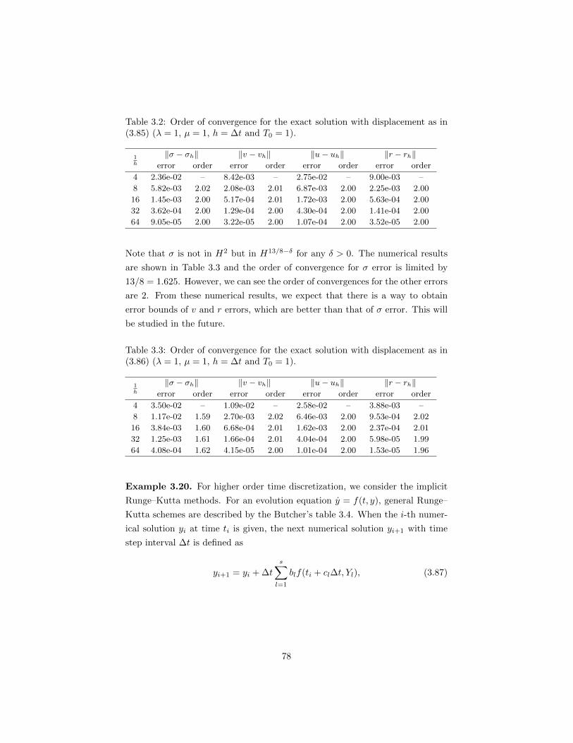
Table 3.2: Order of convergence for the exact solution with displacement as in(3.85) (λ = 1, µ = 1, h = ∆t and T0 = 1).
1h
‖σ − σh‖ ‖v − vh‖ ‖u− uh‖ ‖r − rh‖error order error order error order error order
4 2.36e-02 – 8.42e-03 – 2.75e-02 – 9.00e-03 –
8 5.82e-03 2.02 2.08e-03 2.01 6.87e-03 2.00 2.25e-03 2.00
16 1.45e-03 2.00 5.17e-04 2.01 1.72e-03 2.00 5.63e-04 2.00
32 3.62e-04 2.00 1.29e-04 2.00 4.30e-04 2.00 1.41e-04 2.00
64 9.05e-05 2.00 3.22e-05 2.00 1.07e-04 2.00 3.52e-05 2.00
Note that σ is not in H2 but in H13/8−δ for any δ > 0. The numerical results
are shown in Table 3.3 and the order of convergence for σ error is limited by
13/8 = 1.625. However, we can see the order of convergences for the other errors
are 2. From these numerical results, we expect that there is a way to obtain
error bounds of v and r errors, which are better than that of σ error. This will
be studied in the future.
Table 3.3: Order of convergence for the exact solution with displacement as in(3.86) (λ = 1, µ = 1, h = ∆t and T0 = 1).
1h
‖σ − σh‖ ‖v − vh‖ ‖u− uh‖ ‖r − rh‖error order error order error order error order
4 3.50e-02 – 1.09e-02 – 2.58e-02 – 3.88e-03 –
8 1.17e-02 1.59 2.70e-03 2.02 6.46e-03 2.00 9.53e-04 2.02
16 3.84e-03 1.60 6.68e-04 2.01 1.62e-03 2.00 2.37e-04 2.01
32 1.25e-03 1.61 1.66e-04 2.01 4.04e-04 2.00 5.98e-05 1.99
64 4.08e-04 1.62 4.15e-05 2.00 1.01e-04 2.00 1.53e-05 1.96
Example 3.20. For higher order time discretization, we consider the implicit
Runge–Kutta methods. For an evolution equation y = f(t, y), general Runge–
Kutta schemes are described by the Butcher’s table 3.4. When the i-th numer-
ical solution yi at time ti is given, the next numerical solution yi+1 with time
step interval ∆t is defined as
yi+1 = yi + ∆t
s∑l=1
blf(ti + cl∆t, Yl), (3.87)
78

Table 3.4: The Butcher’s table for general Runge–Kutta schemes.
c1 a11 a12 · · · a1s
c2 a21 a22 · · · a2s
......
.... . .
...cs as1 · · · · · · ass
b1 b2 · · · bs
where Ylsl=1 are obtained by solving
Yj = yi + ∆t
s∑l=1
ajlf(ti + cl∆t, Yl), 1 ≤ j ≤ s. (3.88)
A key idea of this numerical scheme is that the Yl is an approximation of y at
ti + cl∆t because (3.88) is analogous to the equation y = f(t, y), and a linear
combination of them with appropriate coefficient can be a good approximation
of y at ti with high accuracy. For more details, we refer [12].
We present numerical results for (3.84) with the 2-stage RadauIIA method
whose Butcher’s table is as in Table 3.5.
Table 3.5: The Butcher’s table for the 2-stage RadauIIA Runge–Kutta scheme.
1/3 5/12 −1/121 3/4 1/4
3/4 1/4
For the s-stage RadauIIA method, the order of convergence in time is 2s−1.
Table 3.6: Order of convergence for the exact solution with displacement in(3.84) (λ = 1, µ = 1, h = ∆t and T0 = 1). The AFW elements of degree 3 andthe 2-stage RadauIIA time discretization are used.
1h
‖σ − σh‖ ‖v − vh‖ ‖u− uh‖ ‖r − rh‖error order error order error order error order
4 1.31e-02 – 1.38e-03 – 2.10e-03 – 3.77e-03 –
8 1.02e-03 3.68 1.78e-04 2.96 2.58e-04 3.02 4.18e-04 3.17
16 9.88e-05 3.37 2.23e-05 3.00 3.25e-05 2.99 5.05e-05 3.05
32 1.14e-05 3.12 2.78e-06 3.00 4.09e-06 2.99 6.28e-06 3.01
64 1.40e-06 3.03 3.46e-07 3.00 5.13e-07 2.99 7.85e-07 3.00
79

Hence the expected order of convergence is 3 if the AFW element of degree 3 is
used. In order to reconstruct numerical displacement, we use the numerical ap-
proximations of v which correspond to Yl in (3.88) in the Runge–Kutta method.
These numerical approximations are byproducts of the Runge–Kutta scheme.
If we denote those terms as Vi+1/3t and V i+1
t in the 2-stage RadauIIA method,
we have
Vi+ 1
3t ≈ v(ti + ∆t/3), V i+1
t ≈ v(ti + ∆t),
in the time step at ti. By Taylor expansions, one can check that
g(a) = g(0) + ag′(0) +a2
2g′′(a/3) + o(a3),
so we define
U i+1 = U i + ∆tV i +∆t2
2Vi+ 1
3t .
The numerical results in Table 3.6 show that the expected convergence rates are
obtained for all errors.
80

Chapter 4
Mixed methods for the
Kelvin–Voigt model of
viscoelasticity
4.1 Introduction
In this chapter, we consider mixed methods for the Kelvin–Voigt model which
is the simplest model of linear viscoelastic solids. The Kelvin–Voigt model itself
is used to model soft tissues in biomedical engineering and is also an important
basis to make more complicated viscoelastic models. Therefore developing a
numerical scheme for the Kelvin–Voigt model is meaningful not only for its
direct applications but also as a landmark when more complicated models of
viscoelastic materials are studied.
There are not many results on mixed methods for the Kelvin–Voigt model.
Quasistatic problems of the Kelvin–Voigt model, meaning that the mass density
in equations is vanishing, were studied by Rognes and Winther [44] but, to our
knowledge, no one has studied fully dynamic problems of it. In the work of
Rognes and Winther, they suggest a mixed method framework for the Kelvin–
Voigt model using weak symmetry of stress and show a priori error analysis for
the AFW elements and a variant of the lowest order AFW element modified by
Falk (see [10, 30]).
In this chapter, using the mixed method framework in [44], we study mixed
81

methods for the Kelvin–Voigt model with a positive mass density. We prove a
priori error estimates for the AFW and GG elements. The rest of this chapter
is organized as follows. In section 4.2, we establish a velocity-stress weak for-
mulation of the Kelvin–Voigt model with weak symmetry of stress. In section
4.3, we show an error analysis of semidiscrete solutions for the AFW elements.
In section 4.4, we show an error analysis of fully discrete solutions for the AFW
elements. In section 4.5, we show an error analysis for the GG elements and
present a postprocessing technique to improve accuracy of numerical solutions of
displacement. In section 4.6, we present some numerical results which support
our error analysis.
4.2 Weak formulations with weak symmetry
Let u be the displacement vector. As we have seen in (2.8), there are two stresses
related to spring and dashpot units in the Kelvin–Voigt model, and they are
called elastic and viscous stresses, respectively. By (2.8), the elastic and viscous
stresses have the relations
σ0 = C0ε(u), σ1 = C1ε(u),
with rank 4 tensors C0 and C1 which satisfy (2.6) and are uniformly bounded
above and below. The total stress is σ0 + σ1 = C0ε(u) + C1ε(u), and by the
balance law of linear momentum, we have
ρu− div(C0ε(u) + C1ε(u)) = f, (4.1)
for an external body force f . Throughout the discussion in this chapter, we
assume that the mass density ρ satisfies 0 < ρ0 ≤ ρ ≤ ρ1 <∞ for constants ρ0,
ρ1.
To have a velocity-stress weak formulation, we use v = u, σ0 = C0ε(u),
σ1 = C1ε(u) as unknowns. Then we have equations of the Kelvin–Voigt model
as
A0σ0 = A1σ1 = ε(v), ρv − div(σ0 + σ1) = f, (4.2)
where A0 = C−10 , A1 = C−1
1 . We assume the homogeneous displacement bound-
ary conditions u ≡ 0, so v ≡ 0, on ∂Ω for simplicity.
82
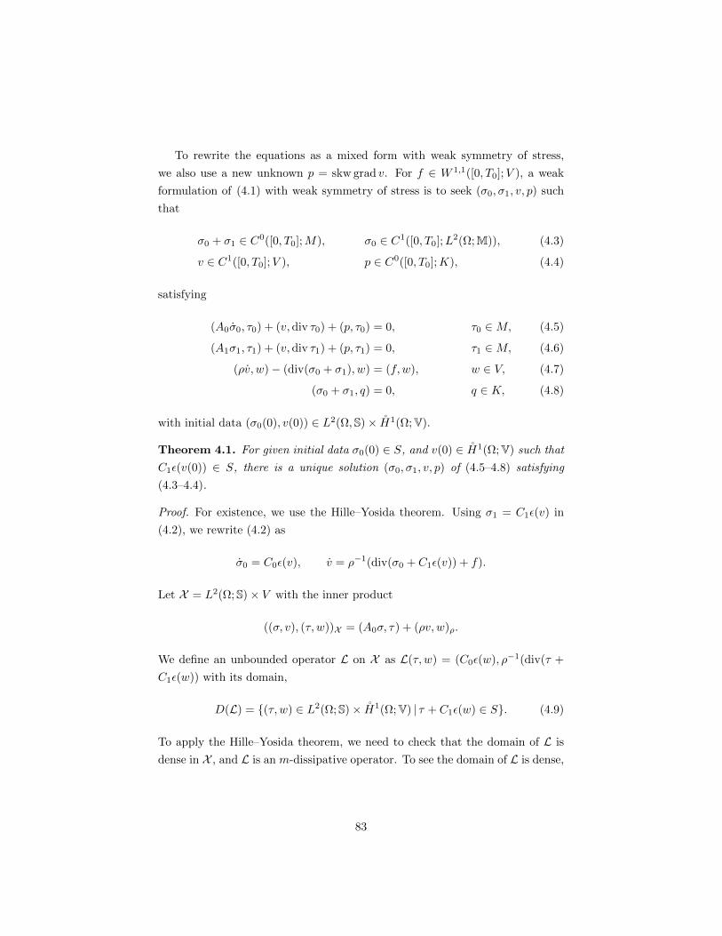
To rewrite the equations as a mixed form with weak symmetry of stress,
we also use a new unknown p = skw grad v. For f ∈ W 1,1([0, T0];V ), a weak
formulation of (4.1) with weak symmetry of stress is to seek (σ0, σ1, v, p) such
that
σ0 + σ1 ∈ C0([0, T0];M), σ0 ∈ C1([0, T0];L2(Ω;M)), (4.3)
v ∈ C1([0, T0];V ), p ∈ C0([0, T0];K), (4.4)
satisfying
(A0σ0, τ0) + (v,div τ0) + (p, τ0) = 0, τ0 ∈M, (4.5)
(A1σ1, τ1) + (v,div τ1) + (p, τ1) = 0, τ1 ∈M, (4.6)
(ρv, w)− (div(σ0 + σ1), w) = (f, w), w ∈ V, (4.7)
(σ0 + σ1, q) = 0, q ∈ K, (4.8)
with initial data (σ0(0), v(0)) ∈ L2(Ω,S)× H1(Ω;V).
Theorem 4.1. For given initial data σ0(0) ∈ S, and v(0) ∈ H1(Ω;V) such that
C1ε(v(0)) ∈ S, there is a unique solution (σ0, σ1, v, p) of (4.5–4.8) satisfying
(4.3–4.4).
Proof. For existence, we use the Hille–Yosida theorem. Using σ1 = C1ε(v) in
(4.2), we rewrite (4.2) as
σ0 = C0ε(v), v = ρ−1(div(σ0 + C1ε(v)) + f).
Let X = L2(Ω; S)× V with the inner product
((σ, v), (τ, w))X = (A0σ, τ) + (ρv, w)ρ.
We define an unbounded operator L on X as L(τ, w) = (C0ε(w), ρ−1(div(τ +
C1ε(w)) with its domain,
D(L) = (τ, w) ∈ L2(Ω;S)× H1(Ω;V) | τ + C1ε(w) ∈ S. (4.9)
To apply the Hille–Yosida theorem, we need to check that the domain of L is
dense in X , and L is an m-dissipative operator. To see the domain of L is dense,
83

let us define
H1(div) = w ∈ H1(Ω;V) |C1ε(w) ∈ S.
It is obvious that S × H1(div) is a subset of the domain of L, so it suffices to
show that S× H1(div) is dense in X . Since S is dense in L2(Ω; S), we only need
to show that H1(div) is dense in V .
For given g ∈ H−1(Ω;V), consider the equation
(C1ε(v), ε(w)) = (g, w), w ∈ H1(Ω;V). (4.10)
By the coercivity of C1, Korn’s inequality, and the Lax–Milgram lemma, this
equation gives a bijective map L : H1(Ω;V) → H−1(Ω;V). Since L and L−1
are bounded by the open mapping theorem, a dense set in H1(Ω;V) is mapped
to a dense set in H−1(Ω;V) and vice versa. For g ∈ V , consider the solution
v of (4.10) and one sees that divC1ε(v) = g in the sense of distributions and
v ∈ H1(div). Therefore the L−1 operator maps V to a subset of H1(div). As
V is dense in H−1(Ω;V), so is H1(div) in H1(Ω;V).
The closedness of the operator L is not difficult to check, so we omit details.
To show L is m-dissipative, we first check that for λ > 0,
((I − λL)(σ, v), (σ, v))X = ‖σ‖2A0+ ‖v‖2ρ − λ(ε(v), σ)− λ(div(σ + C1ε(v)), v)
= ‖σ‖2A0+ ‖v‖2ρ + λ(C1ε(v), ε(v))
≥ ‖(σ, v)‖2X ,
so ‖(I − λL)(σ, v)‖X ≥ ‖(σ, v)‖X . Now we check that I − λL : D(L) → X is
surjective. For given (η, z) ∈ X , we find (σ, v) ∈ D(L) satisfying
σ − λC0ε(v) = η, v − ρ−1(div σ + C1ε(v)) = z.
In the first equation, we get a constraint σ = λC0ε(v) + η. We can obtain
v−ρ−1(div(λC0ε(v)+η)+C1ε(v)) = z by substituting σ in the second equation
using the aforementioned constraint. Rewriting in a weak form, we first find
v ∈ H1(Ω;V) such that
(v, w)ρ + (λC0ε(v) + η + C1ε(v), ε(w)) = (z, w)ρ, w ∈ H1(Ω;V).
Existence of solutions of this equation is a consequence of Korn’s inequality,
84

coercivity of C0 and C1, and the Lax–Milgram lemma. For the solution v,
σ = λC0ε(v) + η from the previous constraint, and the above equation implies
that σ + C1ε(v) ∈ S, i.e., (σ, v) ∈ D(L). Thus I − λL is surjective.
By the Hille–Yosida theorem, for initial data (σ0(0), v(0)) in D(L), there is
a solution of (4.2) such that
(σ0, v) ∈ C0([0, T0];D(L)) ∩ C1([0, T0];X ),
and σ1, p are defined to be σ1 = C1ε(v), p = skw grad v. From these definitions
and Lemma 2.20, we can see that (σ0, σ1, v, p) satisfies (4.5–4.8), so existence is
proved.
For uniqueness, suppose that there are two solutions for same initial data,
and we use (σd0 , σd1 , v
d, pd) to denote the difference of the solutions. Then
(σd0 , σd1 , v
d, pd) satisfies (4.5–4.8) and σd0(0) = 0 = vd(0). Taking τ0 = σ0,
τ1 = σ1, w = v, q = −p in (4.5–4.8), and adding all of them, we get
1
2
d
dt‖σd0‖2A0
+ ‖σd1‖2A1+
1
2
d
dt‖vd‖2ρ = 0.
By integrating and using the fundamental theorem of calculus,
‖σd0(t)‖2A0+ ‖vd(t)‖2ρ +
∫ t
0
‖σd1(s)‖2A1ds = 0,
so σd0 = vd = σd1 ≡ 0. Since pd = skw grad vd, pd ≡ 0 as well. Thus uniqueness
is proved and the proof is completed.
Remark 4.2. The homogeneous displacement boundary conditions v = 0 can be
generalized to inhomogeneous boundary conditions v = g on ∂Ω. Then (4.5) in
the weak formulation is changed to be
(A0σ0, τ0) + (A1σ1, τ1) + (div(τ0 + τ1), v) + (p, τ0 + τ1)
=
∫∂Ω
((τ0 + τ1)ν, g) dS, (4.11)
where ν is the outward unit normal vector field on ∂Ω.
85

4.3 Semidiscrete problems
We show that semidiscrete problems of the Kelvin–Voigt model is well-posed
for the AFW elements. We also state and prove a priori error estimates.
4.3.1 Existence and uniqueness of semidiscrete solutions
Let (Mh, Vh,Kh) be the AFW elements of degree k ≥ 1. We seek σ0,h ∈C1([0, T0];Mh), σ1,h ∈ C0([0, T0];Mh), vh ∈ C1([0, T0];Vh), ph ∈ C0([0, T0];Kh)
in the semidiscrete problem of Kelvin–Voigt model such that
(A0σ0,h, τ0) + (div τ0, vh) + (ph, τ0) = 0, (4.12)
(A1σ1,h, τ1) + (div τ1, vh) + (ph, τ1) = 0, (4.13)
(ρvh, w)− (div(σ0,h + σ1,h), w) = (f, w), (4.14)
(σ0,h + σ1,h, q) = 0, (4.15)
for all (τ0, τ1, w, q) ∈Mh ×Mh × Vh ×Kh with given initial data σ0,h(0) ∈Mh,
vh(0) ∈ Vh.
Theorem 4.3. For given σ0,h(0) ∈Mh, vh(0) ∈ Vh, the system (4.12–4.15) has
a unique solution.
Proof. Let φi, ψi, χi be bases of Mh, Vh, and Kh, respectively. We use
A0, A1, B, C , M , D to denote the matrices whose (i, j)-entries are
(A0φj , φi), (A1φj , φi), (div φj , ψi), (φj , χi), (ρψj , ψi), (ψj , ψi),
respectively. We write σ0,h =∑i αiφi, σ1,h =
∑i βiφi, vh =
∑i γiψi, ph =∑
i ζiχi, Phf = ξiψi, and use α, β, γ, ζ, ξ to denote the coefficient vectors.
Then, based on a new order of unknowns (σ0,h, vh, σ1,h, ph), we may rewrite
(4.12–4.15) as a matrix equation of the formA0 0 0 0
0 M 0 0
0 0 0 0
0 0 0 0
α
γ
β
ζ
=
0 −BT 0 −C T
B 0 B 0
0 −BT A1 −C T
−C 0 −C 0
α
γ
β
ζ
+
0
Dξ
0
0
.
(4.16)
We use Lemma 2.17 to show existence and uniqueness of solutions of this system.
86
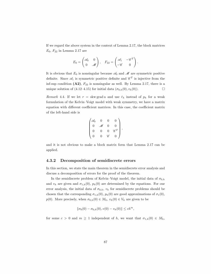
If we regard the above system in the context of Lemma 2.17, the block matrices
E0, F22 in Lemma 2.17 are
E0 =
(A0 0
0 M
), F22 =
(A1 −C T
−C 0
).
It is obvious that E0 is nonsingular because A0 and M are symmetric positive
definite. Since A1 is symmetric positive definite and C T is injective from the
inf-sup condition (A2), F22 is nonsingular as well. By Lemma 2.17, there is a
unique solution of (4.12–4.15) for initial data (σ0,h(0), vh(0)).
Remark 4.4. If we let r = skw gradu and use rh instead of ph for a weak
formulation of the Kelvin–Voigt model with weak symmetry, we have a matrix
equation with different coefficient matrices. In this case, the coefficient matrix
of the left-hand side is A0 0 0 0
0 M 0 0
0 0 0 C T
0 0 C 0
,
and it is not obvious to make a block matrix form that Lemma 2.17 can be
applied.
4.3.2 Decomposition of semidiscrete errors
In this section, we state the main theorem in the semidiscrete error analysis and
discuss a decomposition of errors for the proof of the theorem.
In the semidiscrete problem of Kelvin–Voigt model, the initial data of σ0,h
and vh are given and σ1,h(0), ph(0) are determined by the equations. For our
error analysis, the initial data of σ0,h, vh for semidiscrete problems should be
chosen that the corresponding σ1,h(0), ph(0) are good approximations of σ1(0),
p(0). More precisely, when σ0,h(0) ∈Mh, vh(0) ∈ Vh are given to be
‖σ0(0)− σ0,h(0), v(0)− vh(0)‖ ≤ chm,
for some c > 0 and m ≥ 1 independent of h, we want that σ1,h(0) ∈ Mh,
87

ph(0) ∈ Kh corresponding to them satisfy
‖σ1(0)− σ1,h(0), p(0)− ph(0)‖ ≤ c′hm,
for some c′ > 0 independent of h. We claim that there exists such initial
data (σ0,h(0), vh(0)) which is computable for implementations. Recall that
(σ1(0), v(0), p(0)) satisfies
(A1σ1(0), τ) + (div τ, v(0)) + (τ, p(0)) = 0, (σ1(0), q) = 0, (4.17)
for (τ, q) ∈M ×K from (4.6) at t = 0 and the symmetry of σ1(0). We consider
a solution (σ′h, v′h, p′h) of the system
(A1σ′h, τ) + (div τ, v′h) + (p′h, τ) = 0,
(div σ′h, w) = (div σ1(0), w), (4.18)
(σ′h, q) = 0,
for (τ, w, q) ∈Mh × Vh ×Kh. From (2.32–2.33), we have
‖σ1(0)− σ′h‖+ ‖v(0)− v′h‖+ ‖p(0)− p′h‖ ≤ chm‖σ1(0), v(0), p(0)‖m, (4.19)
for 1 ≤ m ≤ k and Ph div σ1(0) = div σ′h. Note that σ′h, v′h, p′h are computable
quantities by (4.18) when div σ1(0) = divC1ε(v(0)) is known.
Theorem 4.5. Let (Mh, Vh,Kh) be the AFW elements of degree k ≥ 1. Suppose
that σ0, v ∈ W 2,1([0, T0];Hm), σ1, p ∈ W 1,1([0, T0];Hm) and suppose also that
(σ0,h, σ1,h, vh, ph) is the semidiscrete solution of (4.12–4.15) with initial data
σ0,h(0) = Πhσ0(0), vh(0) = v′h,
for which v′h defined by (4.18). Then we have
‖σ0 − σ0,h, σ1 − σ1,h, v − vh, p− ph‖L∞L2
≤ chm(‖σ0, v‖W 2,1Hm + ‖σ1, p‖W 1,2Hm),
for 1 ≤ m ≤ k, where c depends on the time interval T0, elastic and viscous
compliance tensors A0, A1, and the lower and upper bound of the mass density
ρ0, ρ1 but is independent of h.
88

In order to prove Theorem 4.5, we decompose errors into the projection and
approximation errors. We use eσ0 , eσ1 , ev, and ep to denote the semidiscrete
errors σ0− σ0,h, σ1− σ1,h, v− vh, and p− ph, respectively. The error equations
are
(A0eσ0, τ0) + (div τ0, ev) + (ep, τ0) = 0, (4.20)
(A1eσ1 , τ1) + (div τ1, ev) + (ep, τ1) = 0, (4.21)
(ρev, w)− (div(eσ0+ eσ1
), w) = 0, (4.22)
(eσ0+ eσ1
, q) = 0, (4.23)
for (τ0, τ1, w, q) ∈Mh ×Mh × Vh ×Kh. We define (σP0,h, σP1,h, v
Ph , p
Ph ) by
σP0,h = Πhσ0, σP1,h = Πhσ1, vPh = Phv, pPh = P ′hp, (4.24)
and split the semidiscrete errors into
eσi= ePσi
+ ehσi:= (σi − σPi,h) + (σPi,h − σi,h), i = 0, 1,
ev = ePv + ehv := (v − vPh ) + (vPh − vh), (4.25)
ep = ePp + ehp := (p− pPh ) + (pPh − ph),
where eP and eh terms are called the projection and approximation errors,
respectively.
4.3.3 Projection error estimates for the AFW elements
We state the projection error estimates but we omit the proof of this theorem
because it is almost same as the one of Theorem 3.5.
Theorem 4.6. Let (Mh, Vh,Kh) be the AFW elements of degree k ≥ 1 and
suppose that (σ0,h, σ1,h, vh, ph) is a semidiscrete solution of (4.12–4.15). For the
projection errors ePσ0, ePσ1
, ePv , ePp , defined in (4.25), we get
‖ePσ0, ePσ1‖L∞L2 ≤ chm‖σ0, σ1‖L∞Hm , 1 ≤ m ≤ k + 1,
‖ePv , ePp ‖L∞L2 ≤ chm‖v, p‖L∞Hm , 0 ≤ m ≤ k.
Similar results hold for time derivatives of σi, v, and p for i = 0, 1.
89

4.3.4 Approximation error estimates for the AFW ele-
ments
We show a priori estimates of the approximation errors.
Theorem 4.7. Suppose that (σ0, σ1, v, p) is a solution of (4.5–4.8) with the reg-
ularity assumptions in Theorem 4.5 and let ehσ0, ehσ1
, ehv , ehp be the approximation
errors defined in (4.25). Then, for 1 ≤ m ≤ k,
‖ehσ0, ehσ1
, ehv , ehp‖L∞L2 ≤ chm(‖σ0, v‖W 2,1Hm + ‖σ1, p‖W 1,2Hm), (4.26)
where c depends on T0, ρ1, A0, A1 but is independent of h.
Proof. We claim that, for 1 ≤ m ≤ k, it is enough to prove
‖ehσ0, ehv‖L∞L2 ≤ chm(‖v(0)‖m + max‖σ1, p‖L2Hm , ‖σ0, v, p‖L1Hm), (4.27)
‖ehσ0‖L∞L2 ≤ c(‖ehσ0
(0)‖+ ‖ehv (0)‖ρ + hm max‖σ1, p‖L2Hm , ‖σ0, v, p‖L1Hm),(4.28)
‖ehσ1, ehp‖L∞L2 ≤ c‖ehσ0
, ePσ0, ePσ1
, ePp ‖L∞L2 , (4.29)
‖ehσ0(0)‖+ ‖ehv (0)‖ρ ≤ chm‖σ0(0), σ1(0), v(0)‖m. (4.30)
Note that (4.27) gives (4.26) for ehσ0and ehv . From the estimates (4.28) and
(4.30), we have ‖ehσ0‖L∞L2 ≤ chm(‖σ0, v‖W 2,1Hm + ‖σ1, p‖W 1,2Hm). If we com-
bine this estimate with (4.29) and use Theorem 4.6, then (4.26) for ehσ1, ehp
follows.
Now we begin proving (4.27–4.30). We first derive reduced error equations.
Rewriting (4.20–4.22), using the error decomposition in (4.25), we get
(A0(ehσ0+ ePσ0
), τ0) + (div τ0, ehv + ePv ) + (τ0, e
hp + ePp ) = 0,
(A1(ehσ1+ ePσ1
), τ1) + (div τ1, ehv + ePv ) + (τ1, e
hp + ePp ) = 0,
(ρ(ehv + ePv ), w)− (div(ehσ0+ ePσ0
+ ehσ1+ ePσ1
), w) = 0,
(eσ0 + eσ1 , q) = 0,
for (τ0, τ1, w) ∈ Mh × Mh × Vh. Note that (div(ePσ0+ ePσ1
), w), (div τ0, ePv ),
(div τ1, ePv ), and (ePσ0
+ ePσ1, q) vanish from the same argument as in (3.24).
90

Thus
(A0ehσ0, τ0) + (div τ0, e
hv ) + (τ0, e
hp) = −(A0e
Pσ0, τ0)− (τ0, e
Pp ), (4.31)
(A1ehσ1, τ1) + (div τ1, e
hv ) + (τ1, e
hp) = −(A1e
Pσ1, τ1)− (τ1, e
Pp ), (4.32)
(ρehv , w)− (div(ehσ0+ ehσ1
), w) = −(ρePv , w), (4.33)
(ehσ0+ ehσ1
, q) = 0, (4.34)
for (τ0, τ1, w, q) ∈Mh ×Mh × Vh ×Kh.
For (4.27), we take τ0 = ehσ0, τ1 = ehσ1
, w = ehv , q = −ehp in (4.31–4.34) and
add all equations, then,
1
2
d
dt‖ehσ0‖2A0
+ ‖ehσ1‖2A1
+1
2
d
dt‖ehv‖2ρ
= −(A0ePσ0, ehσ0
)− (A1ePσ1, ehσ1
)− (ehσ0+ ehσ1
, ePp )− (ρePv , ehv ).
Using Young’s inequality to (A1ePσ1, ehσ1
) and (ehσ1, ePp ), one can have
−(A1ePσ1
+ ePp , ehσ1
)− ‖ehσ1‖2A1≤ c(‖ePσ1
‖2 + ‖ePp ‖2),
for c > 0 depending only on A0, A1. If we use this inequality to the previous
equality, then one gets
1
2
d
dt‖ehσ0‖2A0
+1
2
d
dt‖ehv‖2ρ
≤ c(‖ePσ1‖2 + ‖ePp ‖2)− (A0e
Pσ0, ehσ0
)− (ehσ0, ePp )− (ρePv , e
hv ). (4.35)
By using a weighted Cauchy–Schwarz inequality, we obtain
1
2
d
dt(‖ehσ0
‖2A0+ ‖ehv‖2ρ) ≤c(‖ePσ1
‖2 + ‖ePp ‖2)
+ c(‖ePσ0‖+ ‖ePp ‖+ ‖ePv ‖)(‖ehσ0
‖2A0+ ‖ehv‖2ρ)
12 .
We apply Lemma 2.14 to this inequality regarding Q = (‖ehσ0‖2A0
+ ‖ehv‖2ρ)1/2,
F = c(‖ePσ0‖+ ‖ePp ‖+ ‖ePv ‖), and G = c(‖ePσ1
‖2 + ‖ePp ‖2). Then, using the facts
ehσ0(0) = 0, ehv (0) = vPh (0)− v′h and the coercivity of A0, we get
‖ehσ0, ehv‖L∞L2 ≤ c‖vPh (0)− v′h‖+ cmax
‖ePσ1
, ePp ‖L2L2 , ‖ePσ0, ePv , e
Pp ‖L1L2
.
If we use the fact ‖vPh (0) − v(0)‖ ≤ chm‖v(0)‖m, (4.19), the projection error
91

estimates in Theorem 4.6, and the triangle inequality, then we have
‖ehσ0, ehv‖L∞L2 ≤ chm(‖v(0)‖+ max‖σ1, p‖L2Hm , ‖σ0, v, p‖L1Hm),
for 1 ≤ m ≤ k, so (4.27) is proved.
For (4.28), we take time derivatives of (4.31–4.34) and use a similar argument
by taking τ0 = ehσ0, τ1 = ehσ1
, w = ehv , and q = −ehp . Following same steps in the
proof of (4.27), we have (4.28).
Now we turn to the proof of (4.29). We first show
‖ehp‖L∞L2 ≤ c‖ehσ1, ePσ1
, ePp ‖L∞L2 . (4.36)
To prove (4.36), by using (A2), we take τ1 in (4.31) such that ‖τ1‖ ≤ c‖ehp‖,div τ1 = 0 and (τ1, q) = (ehp , q) for all q ∈ Kh. Then,
‖ehp‖2 = (τ1, ehp) = −(A1e
hσ1, τ1)− (A1e
Pσ1, τ1)− (τ1, e
Pp ),
and (4.36) is proved by the Cauchy–Schwarz inequality. To complete the proof
of (4.29), now it is enough to show ‖ehσ1‖L∞L2 ≤ c‖ehσ0
, ePσ0, ePσ1‖L∞L2 . For this,
take −τ0 = ehσ1= τ1 in (4.31–4.32) and add them. Then we get
(A1ehσ1, ehσ1
) = −(A0(ehσ0+ ePσ0
), ehσ1)− (A1e
Pσ1, ehσ1
),
and therefore ‖ehσ1‖ ≤ c‖ehσ0
, ePσ0, ePσ1‖, which proves (4.29).
Finally, for (4.30), recall that ehσ0(0) = 0, so div ehσ0
(0) = 0 and
div ehσ1(0) = div Πhσ1(0)− div σ′h = 0.
If we take w = ehv (0) in (4.33), then we have
‖ehv (0)‖2ρ = −(ρePv (0), ehv (0)) ≤ ‖ePv (0)‖ρ‖ehv (0)‖ρ,
so ‖ehv (0)‖ρ ≤ ‖ePv (0)‖ρ ≤ chm‖v(0)‖m for 1 ≤ m ≤ k.
If we take τ0 = −τ1 = ehσ0(0) in (4.31–4.32) and add them, then we get
‖ehσ0(0)‖2A0
= −(A0ePσ0
(0) +A1(ehσ1(0) + ePσ1
(0)), ehσ0(0)).
By the coercivity of A0, the triangle inequality, and the estimate (4.19) with
92

the projection error estimates, we get
‖ehσ0(0)‖ ≤ c‖ePσ0
(0), ehσ1(0), ePσ1
(0)‖ ≤ chm‖σ0(0), σ1(0)‖m,
for 1 ≤ m ≤ k + 1.
4.4 Full discretization
In this section, we consider the error analysis of full discretization with the
Crank–Nicolson scheme.
In semidiscrete problems, we only need initial data of σ0, v. However, if we
use the Crank–Nicolson scheme for full discretization, we need initial data of
σ1 and p as well. Thus we take Σ00 = Πhσ0(0), Σ0
1 = Πhσ1(0), V 0 = Phv(0),
and P 0 = P ′hp(0) as initial data. In full discretization with the Crank–Nicolson
scheme for the equations of Kelvin–Voigt model, initial data of σ1 and v are not
necessarily same as the ones in the semidiscrete problem. In fact, the algebraic
equation of the system involves the arithmetic mean of numerical solutions at
times 0 and ∆t, so the restriction for initial data is not as strong as that in
semidiscrete problems.
In the Crank–Nicolson scheme, (Σj+10 ,Σj+1
1 , V j+1, P j+1), the numerical so-
lution at time tj+1 is defined inductively by
(A0∂tΣj+ 1
20 , τ0) + (div τ0, V
j+ 12 ) + (P j+
12 , τ0) = 0, (4.37)
(A1Σj+ 1
21 , τ1) + (div τ1, V
j+ 12 ) + (P j+
12 , τ0) = 0, (4.38)(
∂tVj+ 1
2 , w)− (div(Σ
j+ 12
0 + Σj+ 1
21 ), w) = (f j+
12 , w), (4.39)
(Σj+ 1
20 + Σ
j+ 12
1 , q) = 0, (4.40)
for (τ0, τ1, w, q) ∈Mh ×Mh × Vh ×Kh and j ≥ 0.
Theorem 4.8. Suppose σ0(0), σ1(0), v(0), p(0) ∈ Hm for 1 ≤ m ≤ k and
σ0, v ∈W 2,1([0, T0];Hm) ∩W 4,1([0, T0];L2),
σ1, p ∈W 1,2([0, T0];Hm) ∩W 3,2([0, T0];L2).(4.41)
For initial data Σ00 = Πhσ0(0), Σ0
1 = Πhσ1(0), V 0 = Phv(0), P 0 = P ′hp(0),
the fully discrete solution (Σj0,Σj1, V
j , P j) in (4.37–4.40) is well-defined and for
93

1 ≤ j ≤ N ,
‖σj0 − Σj0‖+ ‖vj − V j‖+ ‖σj−12
1 − Σj− 1
21 ‖+ ‖pj− 1
2 − P j− 12 ‖
≤ c(∆t2 + hm)(‖σ0, v‖W 2,1Hm∩W 4,1L2 + ‖σ1, p‖W 1,2Hm∩W 3,2L2),
for c > 0 depending on A0, A1, ρ1, T0 but independent of h and ∆t.
The proof will be given in the rest of this section.
4.4.1 Well-definedness
First of all, we show that the full discretization scheme is well-defined. We need
to check when Σj0,Σj1, V
j , P j , f j , f j+1 are given, a solution of the linear system
(4.37–4.40), which is (Σj+10 ,Σj+1
1 , V j+1, P j+1), is well-defined. If we rewrite
(4.37–4.40),
(A0Σj+10 , τ0) +
∆t
2(V j+1,div τ0) +
∆t
2(P j+1, τ0)
= (A0Σj0, τ0)− ∆t
2(V j ,div τ0)− ∆t
2(P j , τ0),
(A1Σj+11 , τ1) + (V j+1,div τ1) + (P j+1, τ1)
= −(A1Σj1, τ1)− (V j ,div τ1)− (P j , τ1),
(V j+1, w)− ∆t
2(div(Σj+1
0 + Σj+11 ), w)
= (V j , w) +∆t
2(div(Σj0 + Σj1), w) + ∆t(f j+
12 , w),
− ∆t
2(Σj+1
0 + Σj+11 , q) =
∆t
2(Σj0 + Σj1, q).
Regarding Σj+10 ,Σj+1
1 , V j+1, P j+1 as unknowns, the above is a system of linear
equations with same number of equations and unknowns. In order to show it is
well-defined, it is enough to show that Σj+10 = Σj+1
1 = V j+1 = P j+1 = 0 when
all of the right-hand side vanish. Suppose all right-hand side terms vanish. If we
take τ0 = Σj+10 , τ1 = Σj+1
1 , w = V j+1, q = P j+1 and add all equations, we have
|Σj+10 |2A0
+ (∆t/2)|Σj+11 |2A1
+ |V j+1|2 = 0 which implies Σj+10 = Σj+1
1 = V j+1 =
0. For P j+1, take τ0 in (4.37) such that (τ0, q) = (P j+1, q) for all q ∈ Kh. Then
the first equation yields |P j+1|2 = 0, so P j+1 = 0 and the fully discrete solution
is well-defined.
94

4.4.2 Convergence
Let us denote the error (σj0 − Σj0, σj1 − Σj1, v
j − V j , pj − P j) by
Ejσi= σji − Σji = (σji − σ
P,ji,h ) + (σP,ji,h − Σji ) =: eP,jσi
+ θjσi, i = 0, 1, (4.42)
Ejv = vj − V j = (vj − vP,jh ) + (vP,jh − V j) =: eP,jv + θjv, (4.43)
Ejp = pj − P j = (pj − pP,jh ) + (pP,jh − P j) =: eP,jp + θjp. (4.44)
In the semidiscrete error analysis of the previous section, we already obtained
error bounds of eP,jσ0, eP,jσ1
, eP,jv , and eP,jp in Theorem 4.6. By the triangle in-
equality, we only need to consider the a priori estimates of θjσ0, θjσ1
, θjv, and
θjp.
Theorem 4.9. Suppose the assumptions of Theorem 4.8 hold. Then there exists
c > 0 which is independent of h and ∆t such that
‖θiσ0‖+ ‖θi−
12
σ1 ‖+ ‖θiv‖+ ‖θi−12
p ‖ ≤ c(∆t2 + hm), (4.45)
for 1 ≤ i ≤ N and 1 ≤ m ≤ k + 1.
Proof. The arithmetic mean of equations (4.5–4.7) at t = tj , tj+1 gives
(A0ˆσj+ 1
20 , τ0) + (div τ0, v
j+ 12 ) + (pj+
12 , τ0) = 0,
(A1σj+ 1
21 , τ1) + (div τ1, v
j+ 12 ) + (pj+
12 , τ1) = 0,
(ρˆvj+12 , w)− (div(σ
j+ 12
0 + σj+ 1
21 ), w) = (f j+
12 , w).
By subtracting (4.37–4.39) from the above three equations and using definitions
of (Eσ0, Eσ1
, Ev, Ep) in (4.42–4.44), we have
(A0∂tEj+ 1
2σ0 , τ0) + (div τ0, E
j+ 12
v ) + (Ej+ 1
2p , τ0) = (A0(∂tσ
j+ 12
0 − ˆσj+ 1
2
0 ), τ0),
(A1Ej+ 1
2σ1 , τ1) + (div τ1, E
j+ 12
v ) + (Ej+ 1
2p , τ1) = 0,
(ρ∂tEj+ 1
2v , w)− (div(E
j+ 12
σ0 + Ej+ 1
2σ1 ), w) = (ρ(∂tv
j − ˆvj+12 ), w).
If we consider (4.42–4.44), and the facts (div τ, ePv ) = (div ePσi, w) = 0, i = 0, 1
for τ ∈ Mh, w ∈ Vh, and adding the first two equations for simplicity, then we
95

get
(A0∂tθj+ 1
2σ0 , τ0) + (A1θ
j+ 12
σ1 , τ1) + (div(τ0 + τ1), θj+ 1
2v ) + (θ
j+ 12
p , τ0 + τ1) (4.46)
= (A0(ωj+ 1
21 + ω
j+ 12
2 ) + ωj+ 1
24 , τ0) + (A1ω
j+ 12
3 + ωj+ 1
24 , τ1),
(ρ∂tθj+ 1
2v , w)− (div(θ
j+ 12
σ0 + θj+ 1
2σ1 ), w) = (ω
j+ 12
5 + ωj+ 1
26 , w), (4.47)
where
ωj+ 1
21 = ∂tσ
j+ 12
0 − ˆσj+ 1
20 , ω
j+ 12
2 = −∂teP,j+ 1
2σ0 , ω
j+ 12
3 = −eP,j+12
σ1 ,
ωj+ 1
24 = −eP,j+
12
p , ωj+ 1
25 = ρ(∂tv
j+ 12 − ˆvj+
12 ), ω
j+ 12
6 = −ρ∂teP,j+ 1
2v .
(4.48)
Letting τ0 = θj+1/2σ0 , τ1 = θ
j+1/2σ1 in (4.46), w = θ
j+1/2v in (4.47), and adding
these equations,
‖θj+1σ0‖2A0
+ 2∆t‖θj+12
σ1 ‖2A1+ ‖θj+1
v ‖2ρ − (‖θjσ0‖2A0
+ ‖θjv‖2ρ) (4.49)
= 2∆t(A0(ωj+ 1
21 + ω
j+ 12
2 ) + ωj+ 1
24 , θ
j+ 12
σ0 )
+ 2∆t(A1ωj+ 1
23 + ω
j+ 12
4 , θj+ 1
2σ1 ) + 2∆t(ω
j+ 12
5 + ωj+ 1
26 , θ
j+ 12
v ).
By Young’s inequality and the coercivity of A1, there is c > 0 independent of h
and ∆t such that
2∆t(A1ωj+ 1
23 + ω
j+ 12
4 , θj+ 1
2σ1 ) ≤ 2∆t‖θj+
12
σ1 ‖2A1+ c∆t(‖ωj+
12
3 ‖2 + ‖ωj+12
4 ‖2).
If we use this inequality to (4.49), then we can get
(‖θj+1σ0‖2A0
+ ‖θj+1v ‖2ρ)− (‖θjσ0
‖2A0+ ‖θjv‖2ρ) (4.50)
≤ 2∆t(A0(ωj+ 1
21 + ω
j+ 12
2 ) + ωj+ 1
24 , θ
j+ 12
σ0 ) + 2∆t(ωj+ 1
25 + ω
j+ 12
6 , θj+ 1
2v )
+ c∆t(‖ωj+12
3 ‖2 + ‖ωj+12
4 ‖2).
By the Cauchy–Schwarz inequality, regarding ‖θjσ0‖2A0
+ ‖θjv‖2ρ as Q2i , we can
96

apply Lemma 2.16 and have one of the followings:
(‖θiσ0‖2A0
+ ‖θiv‖2ρ)12 ≤ c∆t
i−1∑j=0
‖ωj+12
1 , ωj+ 1
22 , ω
j+ 12
4 , ωj+ 1
25 , ω
j+ 12
6 ‖, (4.51)
(‖θiσ0‖2A0
+ ‖θiv‖2ρ)12 ≤ c(∆t) 1
2
i−1∑j=0
(‖ωj+12
3 ‖2 + ‖ωj+12
4 ‖2)
12
. (4.52)
We claim that
∆t
i−1∑j=0
‖ωj+12
1 , ωj+ 1
22 , ω
j+ 12
4 , ωj+ 1
25 , ω
j+ 12
6 ‖ ≤ c(∆t2 + hm), (4.53)
(∆t)12
i−1∑j=0
(‖ωj+12
3 ‖2 + ‖ωj+12
4 ‖2)
12
≤ c(∆t2 + hm), (4.54)
hold and note that these estimates imply (4.45) for θiσ0by the coercivity of A0.
By applying the Taylor expansion (3.53), definitions of ω terms in (4.48),
and the projection error estimates, the estimates (4.53–4.54) are obtained from
the estimates,
∆t‖ωj+12
1 ‖ =1
2‖2σj+1
0 − 2σj0 −∆tσj+10 −∆tσj0‖ ≤ c∆t2
∫ tj+1
tj
‖...σ 0‖ ds, (4.55)
∆t‖ωj+12
5 ‖ =1
2‖ρ(2vj+1 − 2vj −∆tvj+1 −∆tvj)‖ ≤ c∆t2
∫ tj+1
tj
‖...v ‖ ds,
(4.56)
∆t‖ωj+12
2 ‖ = ∆t‖∂teP,j+ 1
2σ0 ‖ =
∥∥∥∥∥∫ tj+1
tj
ePσ0ds
∥∥∥∥∥ ≤ chm∫ tj+1
tj
‖σ0‖m ds, (4.57)
∆t‖ωj+12
6 ‖ = ∆t‖ρ∂teP,j+ 1
2v ‖ =
∥∥∥∥∥∫ tj+1
tj
ρePv ds
∥∥∥∥∥ ≤ chm∫ tj+1
tj
‖v‖m ds, (4.58)
‖ωj+12
3 ‖ = chm‖σ1‖L∞Hm , ‖ωj+12
4 ‖ = chm‖p‖L∞Hm . (4.59)
It is easy to see that (4.55–4.59) imply (4.53). The estimate (4.54) comes from
97

(4.59) with
i−1∑j=0
‖ωj+12
3 ‖2 1
2
≤ cN 12hm‖σ1‖L∞Hm ≤ cT0(∆t)−
12hm‖σ1‖L∞Hm , (4.60)
i−1∑j=0
‖ωj+12
4 ‖2 1
2
≤ cN 12hm‖p‖L∞Hm ≤ cT0(∆t)−
12hm‖p‖L∞Hm . (4.61)
Hence the estimate (4.45) for θiσ0, θiv is proved.
Now we consider estimates in (4.45) for θi+1/2σ1 , and θ
i+1/2p . For the estimate
of θj+1/2σ1 , let −τ0 = τ1 = θ
j+1/2σ1 in (4.46). Then
‖θj+12
σ1 ‖2 ≤ c‖θj+ 1
2σ1 ‖2A1
= c(A0∂tθj+ 1
2σ0 −A0(ω
j+ 12
1 + ωj+ 1
22 ) +A1ω
j+ 12
3 + ωj+ 1
24 , θ
j+ 12
σ1 )
≤ c‖∂tθj+ 1
2σ0 , ω
j+ 12
1 , ωj+ 1
22 , ω
j+ 12
3 , ωj+ 1
24 ‖‖θj+
12
σ1 ‖.
For θj+1/2p , in (4.46), let τ1 = 0 and take τ0 to be div τ0 = 0, (τ0, θ
j+1/2p ) =
‖θj+1/2p ‖2 so that ‖τ0‖ ≤ c‖θj+1/2
p ‖ by Corollary 2.4. Then
‖θj+12
p ‖2 = (−A0∂tθj+ 1
2σ0 + ω
j+ 12
1 + ωj+ 1
22 + ω
j+ 12
3 + ωj+ 1
24 , τ0)
≤ c‖∂tθj+ 1
2σ0 , ω
j+ 12
1 , ωj+ 1
22 , ω
j+ 12
3 , ωj+ 1
24 ‖‖θj+
12
p ‖.
Consequently, we get ‖θj+12
σ1 , θj+ 1
2p ‖ ≤ ‖∂tθ
j+ 12
σ0 , ωj+ 1
21 , ω
j+ 12
2 , ωj+ 1
23 , ω
j+ 12
4 ‖.From the estimates (4.55), (4.57), and (4.59), it suffices to show ‖∂tθj+1/2
σ0 ‖ ≤c(∆t2 + hm) to complete the proof of (4.45).
To estimate ‖∂tθj+1/2σ0 ‖, we consider the differences of (4.46), (4.47) with
indices j and j − 1, which are
∆t(A0∂2t θjσ0, τ0) +
1
2(A1(θj+1
σ1− θj−1
σ1), τ1) +
1
2(div(τ0 + τ1), θj+1
v − θj−1v )
+1
2(θj+1p − θj−1
p , τ0 + τ1) = (A0(ηj1 + ηj2) + ηj4, τ0) + (A1ηj3 + ηj4, τ1), (4.62)
∆t(∂2t θjv, w)− 1
2(div(θj+1
σ0− θj−1
σ0+ θj+1
σ1− θj−1
σ1), w) = (ηj5 + ηj6, w), (4.63)
98

where ηjl = ωj+1/2l − ωj−1/2
l , l = 1, · · · , 6. Let
τ0 =θj+1σ0− θj−1
σ0
∆t, τ1 =
θj+1σ1− θj−1
σ1
∆t, w =
θj+1v − θj−1
v
∆t,
in (4.62) and (4.63), and add them. Then, after cancellations from the facts
Y j+1 − Y j−1
∆t= ∂tY
j+ 12 + ∂tY
j− 12 , ∆t∂2
t Yj = ∂tY
j+ 12 − ∂tY j−
12 ,
for a sequence Y j, we can get
‖∂tθj+ 1
2σ0 ‖2A0
+‖∂tθj+ 1
2v ‖2ρ+∆t‖∂tθ
j+ 12
σ1 +∂tθj− 1
2σ1 ‖2A1
−(‖∂tθj− 1
2σ0 ‖2A0
+‖∂tθj− 1
2v ‖2ρ)
= (A0(ηj1 + ηj2) + ηj4, ∂tθj+ 1
2σ0 + ∂tθ
j− 12
σ0 ) + (A1ηj3 + ηj4, ∂tθ
j+ 12
σ1 + ∂tθj− 1
2σ1 ).
We apply the following inequality, which is obtained from Young’s inequality,
to the above equality,
(A1ηj3 + ηj4, ∂tθ
j+ 12
σ1 + ∂tθj− 1
2σ1 )
≤ ∆t‖∂tθj+ 1
2σ1 + ∂tθ
j− 12
σ1 ‖2A1+ (c/∆t)(‖ηj3‖2 + ‖ηj4‖2),
then we have
(‖∂tθj+ 1
2σ0 ‖2A0
+ ‖∂tθj+ 1
2v ‖2ρ)− (‖∂tθ
j− 12
σ0 ‖2A0+ ‖∂tθ
j− 12
v ‖2ρ)
≤ (A0(ηj1 + ηj2) + ηj4, ∂tθj+ 1
2σ0 + ∂tθ
j− 12
σ0 ) + (c/∆t)(‖ηj3‖2 + ‖ηj4‖2).
By Lemma 2.16, we have either
(‖∂tθi+ 1
2σ0 ‖2A0
+ ‖∂tθi+ 1
2v ‖2ρ)
12
≤ (‖∂tθ12σ0‖2A0
+ ‖∂tθ12v ‖2ρ)
12 +
i−1∑j=0
‖ηj1, ηj2, η
j4, η
j5, η
j6‖,
(4.64)
or
(‖∂tθi+ 1
2σ0 ‖2A0
+ ‖∂tθi+ 1
2v ‖2)
12
≤ (‖∂tθ12σ0‖2A0
+ ‖∂tθ12v ‖2ρ)
12 + c(∆t)−1/2
i−1∑j=0
(‖ηj3‖2 + ‖ηj4‖2)
1/2
.(4.65)
99

Now our goal, the estimate ‖∂tθi+1/2σ0 ‖ ≤ c(∆t2 + hm), is reduced to proving
(‖∂tθ12σ0‖2A0
+ ‖∂tθ12v ‖2ρ)
12 ≤ c(∆t2 + hm), (4.66)
i−1∑j=1
‖ηj1, ηj2, η
j4, η
j5, η
j6‖ ≤ c(∆t2 + hm), (4.67)
i−1∑j=1
(‖ηj3‖2 + ‖ηj4‖2)
12
≤ c(∆t) 12hm. (4.68)
If we use the facts ∂tθ1/2σ0 = θ1
σ0/∆t, ∂tθ
1/2v = θ1
v/∆t, and the inequality (4.51),
then we get
(‖∂tθ12σ0‖2A0
+ ‖∂tθ12v ‖2ρ)
12 ≤ ‖ω
121 , ω
122 , ω
124 , ω
125 , ω
126 ‖.
By (4.55–4.59), we have
‖ω121 ‖ ≤ c∆t2‖
...σ 0‖L∞L2 , ‖ω
125 ‖ ≤ c∆t2‖
...v ‖L∞L2 ,
‖ω122 ‖ ≤ chm‖σ0‖L∞Hm , ‖ω
124 ‖ ≤ chm‖p‖L∞Hm , ‖ω
126 ‖ ≤ chm‖v‖L∞Hm ,
which completes the proof of (4.66).
Now we turn to the proof of (4.67). First, we obtain∑i−1j=0 ‖η
j1‖ ≤ c∆t2 with
c depending on ‖σ(4)‖L1L2 from the Taylor expansion formula (3.54). Similarly,
we have∑i−1j=0 ‖η
j5‖ ≤ c∆t
2 with c depending on ‖v(4)‖L1L2 . We also see
‖ηj2‖ =1
∆t‖eP,j+1σ0
+ eP,j−1σ0
− 2eP,jσ0‖ ≤
∫ tj+1
tj−1
‖ePσ0‖ ds ≤ chm
∫ tj+1
tj−1
‖σ0‖m ds,
‖ηj6‖ =1
∆t‖ρ(eP,j+1
v + eP,j−1v − 2eP,jv )‖ ≤
∫ tj+1
tj−1
‖ρePv ‖ ds ≤ chm∫ tj+1
tj−1
‖v‖m ds,
and conclude that∑m−1j=0 (‖ηj2‖+ ‖ηj6‖) ≤ chm. Note also that
‖ηj4‖ = ‖eP,j+1p − eP,j−1
p ‖ =
∥∥∥∥∥∫ tj+1
tj−1
ePp ds
∥∥∥∥∥ ≤ chm∫ tj+1
tj−1
‖p‖m ds,
so combining all the above estimates of η terms, (4.67) is proved.
100

For (4.68), by the Cauchy–Schwarz inequality, we get
‖ηj3, ηj4‖2 ≤ ch2m
(∫ tj+1
tj−1
‖σ1, p‖mds
)2
≤ c∆th2m
∫ tj+1
tj−1
‖σ1, p‖2m ds,
for each 1 ≤ j ≤ N − 1 and we have
i−1∑j=1
(‖ηj3‖2 + ‖ηj4‖2)
12
≤ cT0(∆t)12hm‖σ1, p‖L2Hm .
Thus we proved (‖∂tσi+1/20 ‖2A0
+ ‖∂tvi+1/2‖2ρ)1/2 ≤ c(∆t2 + hm) and therefore
the proof of (4.45) is completed.
4.5 Error analysis for the GG elements
In this section we discuss the error analysis for the GG elements.
Theorem 4.10. Let (Mh, Vh,Kh) be the GG elements of degree k ≥ 1, m be
an integer of which 1 ≤ m ≤ k + 1, and m′ = m − δm,k+1 where δm,k+1 is the
Kronecker delta. Suppose ‖ρ‖W 1,∞h
<∞ for ‖ρ‖W 1,∞h
defined in (3.64) and
σ0 ∈W 2,1([0, T0];Hm) ∩W 4,1([0, T0];L2),
v ∈W 2,1([0, T0];Hm′) ∩W 4,1([0, T0];L2),
σ1, p ∈W 1,1([0, T0];Hm) ∩W 3,1([0, T0];L2).
(4.69)
Assume the initial data are given to be Σ00 = Πhσ0(0), Σ0
1 = Πhσ1(0), V 0 =
Phv(0), P 0 = P ′hp(0). Then the fully discrete solution (Σj0,Σj1, V
j , P j) in (4.37–
4.39) is well-defined and for all 1 ≤ j ≤ N ,
‖σj0 − Σj0, Phvj − V j , σj−
12
1 − Σj− 1
21 , pj−
12 − P j− 1
2 ‖ (4.70)
≤ c(∆t2 + hm),
‖vj − V j‖ ≤ c(∆t2 + hm′), (4.71)
where the constants c depend on
‖σ0‖W 2,1Hm∩W 4,1L2 , ‖σ1, p‖W 1,2Hm∩W 3,1L2 , ‖v‖W 2,1Hm′∩W 4,1L2 ,
101

and A0, A1, ‖ρ‖W 1,∞h
, T0 but is independent of h and ∆t.
In the previous section, the proof of Theorem 4.8 consists of the proof of well-
definedness of (Σj0,Σj1, V
j , P j) and the proof of error estimates. Since we can
prove that (Σj0,Σj1, V
j , P j) is well-defined with the same argument as before,
we only discuss the a priori error estimates.
For the error estimates, we consider the projection errors (eP,jσ0, eP,jσ1
, eP,jv , eP,jp )
and the approximation errors (θjσ0, θjσ1
, θjv, θjp) as in (4.42–4.44).
Lemma 4.11. There exists a constant c > 0 independent of s and h so that the
following inequalities hold.
‖ePσi‖ ≤ chm‖σi‖m, 1 ≤ m ≤ k + 1, i = 0, 1, (4.72)
‖ePv ‖ ≤ chm‖v‖m, 0 ≤ m ≤ k, (4.73)
‖ePp ‖ ≤ chm‖p‖m, 0 ≤ m ≤ k + 1. (4.74)
Similar estimates hold for the time derivatives of σi, v, p, respectively, as in
Theorem 4.6.
Since the proof of this theorem is almost same as the one of Theorem 3.11,
we omit details. For Theorem 4.10 we only need to consider a priori estimates
of the approximation errors (θjσ0, θjσ1
, θjv, θjp).
Theorem 4.12. Suppose the assumptions in Theorem 4.10 hold and θiσ0, θiσ1
,
θiv, θir are defined as in (4.42–4.44). Then there exists a constant c > 0 inde-
pendent of h and ∆t so that
‖θiσ0, θi− 1
2σ1 , θiv, θ
i− 12
p ‖ ≤ c(∆t2 + hm), 1 ≤ i ≤ N, 1 ≤ m ≤ k + 1. (4.75)
Proof. Since the proof is almost same as the one of Theorem 4.9, we only sketch
it with some explanations of the steps which need to be modified.
For the a priori estimates, we can follow same argument in the proof of
Theorem 4.8 and obtain (4.49). Let ρc be the orthogonal L2 projection of ρ
into the space of piecewise constant functions associated to Th. Define ωj+1/26 =
(ρ− ρc)∂teP,j+1/2v and note that
(ωj+ 1
26 , θ
j+ 12
v ) = (ρ∂teP,j+ 1
2v , θ
j+ 12
v ) = ((ρ− ρc)∂teP,j+ 1
2v , θ
j+ 12
v ) = (ωj+ 1
26 , θ
j+ 12
v ),
because ρc∂teP,j+1/2v ⊥ Vh from the definition of ∂te
P,j+1/2v and the fact that
eP,jv ⊥ Vh for all 0 ≤ j ≤ N . Therefore we have an equality analogous to (4.50)
102

as
‖θj+1σ0‖2A0
+ 2∆t‖θj+12
σ1 ‖2A1+ ‖θj+1
v ‖2ρ − (‖θjσ0‖2A0
+ ‖θjv‖2ρ)
= 2∆t(A0(ωj+ 1
21 + ω
j+ 12
2 ) + ωj+ 1
24 , θ
j+ 12
σ0 )
+ 2∆t(A1ωj+ 1
23 + ω
j+ 12
4 , θj+ 1
2σ1 ) + 2∆t(ω
j+ 12
5 + ωj+ 1
26 , θ
j+ 12
v ).
Repeating the steps from (4.50) to (4.52), we need to show
c∆t
i−1∑j=0
‖ωj+12
1 , ωj+ 1
22 , ω
j+ 12
4 , ωj+ 1
25 , ω
j+ 12
6 ‖ ≤ c(∆t2 + hm), (4.76)
(∆t)1/2
i−1∑j=0
(‖ωj+12
3 ‖2 + ‖ωj+12
4 ‖2)
12
≤ c(∆t2 + hm), (4.77)
for 1 ≤ m ≤ k + 1, to prove (4.75) for ‖θiσ0‖ and ‖θiv‖.
In order to show (4.76), we use (4.55–4.57) and (4.59) for the estimates of
ωj+1/2l , l = 1, · · · 5. For ω
j+1/26 , we use
∆t‖ωj+12
6 ‖ = ∆t‖(ρ− ρc)∂tvP,j‖ =
∥∥∥∥∥∫ tj+1
tj
(ρ− ρc)(vPh − v) ds
∥∥∥∥∥≤ chm+1‖ρ‖W 1,∞
h
∫ tj+1
tj
‖v‖m ds, 1 ≤ m ≤ k.
In order to show (4.77), we can use (4.60–4.61).
For the proof of (4.75) for ‖θi−1/2σ1 , θ
i−1/2p ‖, we repeat the argument in the
proof of Theorem 4.9 with the only difference that ωj+1/26 is replaced by ω
j+1/26 .
Since the proof is same, we omit details.
We also show that a simple postprocessing can be used to find a more accu-
rate numerical solution of v. As we have done in elastodynamics problem in the
previous chapter, for Vh in the GG elements, let V ∗h be the space of (possibly
discontinuous) piecewise polynomials of one degree higher than Vh and Vh be
the orthogonal complement of Vh in V ∗h . The orthogonal L2 projections onto
V ∗h and Vh are denoted by P ∗h and Ph, respectively.
Theorem 4.13. For simplicity, we assume that Theorem 4.10 holds with m =
103

k + 1 and ‖v‖W 2,1Hk+1∩W 4,1L2 <∞. We define v∗,i+1/2h ∈ V ∗h to be
(gradh v∗,i+ 1
2
h , gradh w) = (A1Σi+ 1
21 + P i+
12 , gradh w), w ∈ Vh, (4.78)
(v∗,i+ 1
2
h , w) = (V i+12 , w), w ∈ Vh, (4.79)
where gradh is the piecewise gradient operator adapted to the triangulation Thfor each 0 ≤ i ≤ N − 1. Then for each 0 ≤ i ≤ N − 1,
‖v∗,i+12
h − vi+ 12 ‖
≤ c(∆t2 + hk+1)(‖σ0, v‖W 2,1Hk+1∩W 4,1L2 + ‖σ1, p‖W 1,1Hk+1∩W 3,1L2).
We do not show its proof here because it is almost same as that of Theorem
3.13 with minor modifications.
4.6 Numerical results
We present numerical results in this section. For numerical computations, we
use Ω = [0, 1] × [0, 1] and the AFW elements of degree k = 2 in all of our
numerical computations. We assume that the medium is homogeneous with
density ρ = 1, and the constitutive equations for A0 and A1 are the forms of
isotropic materials introduced in (2.7) with constants λ0, λ1, µ0, and µ1. For
each mesh size h, we take ∆t = h for time step ∆t and the expected order of
convergence from our analysis is 2. All numerical results are about the L2 errors
at time T0 = 1.
Although we only proved that error estimates of σ1, and p at the midpoints
of time steps are O(∆t2 +hm), it is not difficult to show, using trapezoidal rule,
that error bounds of same order of accuracy can be obtained at tj , 1 ≤ j ≤ N .
The implementations are done using Dolfin Python module [1] of FEniCS
project [2, 38].
Example 4.14. Consider the displacement field
u(t, x, y) =
(sin t sin(πx) sin(πy)
sin tx(1− x)y(1− y)
), (4.80)
and boundary conditions are the homogeneous displacement boundary condi-
tions. The numerical result for (4.81) is in Table 4.1.
104

Example 4.15. As an example of inhomogeneous displacement boundary con-
ditions, we use
u(t, x, y) =
(e−y sinx cos t
et+x
), (4.81)
and the variational form proposed in (4.11) is used. The numerical results are
shown in Table 4.2. We see that the order of convergence is same as that in our
error analysis.
Example 4.16. For a nonsmooth solution with inhomogeneous displacement
boundary conditions, we consider a solution with displacement
u(t, x, y) =
(x
73 cos t
x73 (1 + t2)
). (4.82)
Then the corresponding σ0, σ1, p are
σ0 =
(0 7
3 (x43 (1 + t2) + y
43 cos t)
73 (x
43 (1 + t2) + y
43 cos t) 0
),
σ1 =
(0 70
3 (2tx43 − y 4
3 sin t)703 (2tx
43 − y 4
3 sin t) 0
),
p =
(0 − 7
6 (2tx43 + y
43 sin t)
76 (2tx
43 + y
43 sin t) 0
),
so they are in H11/6−δ in space for any δ > 0. We again use the variational form
proposed in (4.11), and the numerical results are shown in Table 4.3. We can
see that the orders of convergence of σ0, σ1, p errors are limited by 11/6 ≈ 1.83
but the order of convergence of v error is still 2. As in the nonsmooth solution
Table 4.1: Order of convergence for displacement as in (4.80) (λ0 = µ0 = 1,λ1 = µ1 = 10, h = ∆t and T0 = 1).
1h
‖σ0 − σ0,h‖ ‖σ1 − σ1,h‖ ‖v − vh‖ ‖p− ph‖error order error order error order error order
4 6.76e-02 – 4.05e-01 – 1.04e-02 – 1.59e-02 –
8 1.38e-02 2.29 7.19e-02 2.49 2.67e-03 1.96 4.15e-03 1.94
16 3.19e-03 2.11 1.57e-02 2.19 6.74e-04 1.98 1.06e-03 1.97
32 7.78e-04 2.04 3.76e-03 2.06 1.69e-04 1.99 2.67e-04 1.99
64 1.93e-04 2.01 9.28e-04 2.02 4.24e-05 2.00 6.69e-05 2.00
105

Table 4.2: Order of convergence for displacement as in (4.81) (λ0 = µ0 = 1,λ1 = µ1 = 10, h = ∆t and T0 = 1).
1h
‖σ0 − σ0,h‖ ‖σ1 − σ1,h‖ ‖v − vh‖ ‖p− ph‖error order error order error order error order
4 2.27e-02 – 6.65e-02 – 8.25e-03 – 4.58e-03 –
8 5.64e-03 2.01 1.55e-02 2.10 2.04e-03 2.02 1.12e-03 2.03
16 1.41e-03 2.00 3.73e-03 2.06 5.06e-04 2.01 2.78e-04 2.01
32 3.52e-04 2.00 9.14e-04 2.03 1.26e-04 2.01 6.92e-05 2.01
64 8.79e-05 2.00 2.26e-04 2.02 3.14e-05 2.00 1.72e-05 2.00
Table 4.3: Order of convergence for displacement as in (4.82) (λ0 = µ0 = 1,λ1 = µ1 = 10, h = ∆t and T0 = 1).
1h
‖σ0 − σ0,h‖ ‖σ1 − σ1,h‖ ‖v − vh‖ ‖p− ph‖error order error order error order error order
4 5.34e-02 – 6.42e-01 – 3.69e-02 – 2.02e-02 –
8 1.58e-02 1.76 1.85e-01 1.80 9.04e-03 2.03 6.20e-03 1.70
16 4.54e-03 1.80 5.25e-02 1.82 2.23e-03 2.02 1.83e-03 1.76
32 1.28e-03 1.82 1.48e-02 1.82 5.55e-04 2.01 5.25e-04 1.80
64 3.61e-04 1.83 4.18e-03 1.83 1.38e-04 2.00 1.50e-04 1.81
example for elastodynamics, this result gives a motivation to find a better error
analysis for v error.
106

Chapter 5
Mixed methods for the
Maxwell and generalized
Zener models
5.1 Introduction
In this chapter, we consider mixed methods for the Maxwell and generalized
Zener models. We use a unified framework such that the Maxwell model is a
special case of the Zener model, so we shall show a complete analysis only for
the Zener model. Since the generalized Zener model is a parallel connection of
multiple Zener components, it is straightforward to extend our analysis to the
generalized Zener model.
Although equations of the Maxwell and Zener models are similar in our
framework, they represent very different physical features. The Maxwell model
is the simplest model for viscoelastic fluids, but the Zener model, which is also
called the standard linear solid model, is a model one for viscoelastic solids.
There are several previous works for these two models using mixed methods.
In [16], Becache, Joly, and Tsogka studied a priori error analysis and PML
implementation of Zener model with strongly symmetric rectangular elements
developed in [15]. They used a generalized Kelvin–Voigt form of the Zener
model and the difference of elastic and viscoelastic stresses is used as an internal
variable for mixed formulation. In [44], Rognes and Winther studied quasistatic
107

problems, i.e., mass density is vanishing, of the Maxwell model with the Arnold–
Falk–Winther elements and a modified Arnold–Falk–Winther elements by Falk
[30]. They suggested a unified framework for the Maxwell and Zener models
that we adopt here but they did not show an analysis of the Zener model and
did not cover problems with nonvanishing mass densities.
In this chapter, we show the a priori error analysis of the Zener model for the
AFW and GG elements. We point out that our numerical scheme, compared
to the previous study in [16], is advantages from several viewpoints. First, we
use triangular finite elements, so our method is easy to apply to problems on
domains with more general geometry. Secondly, we use the Crank–Nicolson
scheme for time discretization which is absolutely stable whereas the leap-frog
type scheme in [16] needs a CFL condition for stability. The CFL condition in
[16] depends on material parameters and the constant of CFL condition may not
be easily obtained in anisotropic materials. In particular, the constant of CFL
condition in [16] is very small when the Lame coefficient λ of material is large.
However, the time discretization in our numerical scheme is unconditionally
stable and can be used without concerning the range of material parameters.
The organization of this chapter is the following. In section 5.2, we derive
the governing equations of the models we are interested in and rewrite them in
velocity-stress weak forms with weak symmetry of stress. In sections 5.3 and
5.4, we show the a priori error analysis of the semidiscrete and fully discrete
solutions for the AFW elements. In section 5.5, we carry out the a priori error
analysis for the GG elements. Finally, in section 5.6, we present numerical
results which support our error analysis.
5.2 Weak formulations with weak symmetry
In this section, we only discuss a weak formulation of the Zener model with
weak symmetry of stresses in detail. Since the Maxwell model is a special case
of the Zener one, we will only briefly explain it after we derived a velocity-stress
mixed form of the Zener model.
We recall the description of Zener model in Figure 2.1 as a mechanical model.
For the displacement u, let u = u0 +u1 where u0, u1 are the displacement parts
involved in the spring and dashpot of the Maxwell component in the Zener
model. The stresses from the Maxwell component and from the other spring
unit, are denoted by σ0 and σ1. Then the total stress is σ := σ0 + σ1.
108

By (2.8), σ1 = C1ε(u) for the spring unit. In the Maxwell component,
σ0 = C0ε(u0) = C ′0ε(u1) where C0, C ′0 are the stiffness tensor given by the spring
and dashpot units in the Maxwell component. Let A0, A′0, A1 be the inverses
of C0, C ′0, C1. Then we have A1σ1 = ε(u), A0σ0 = ε(u0), and A′0σ0 = ε(u1).
By adding the second and third equations and using u = u0 + u1,
A0σ0 +A′0σ0 = ε(u), A1σ1 = ε(u),
and from the balance of linear momentum, ρu−div(σ0 +σ1) = f for an external
body force f . We assume that 0 < ρ0 ≤ ρ ≤ ρ1 <∞ for constants ρ0, ρ1. Thus
the equations of the Zener model are
A0σ0 +A′0σ0 = ε(u), A1σ1 = ε(u), ρu− div(σ0 + σ1) = f. (5.1)
We only consider the problems with homogeneous displacement boundary con-
ditions u ≡ 0 on ∂Ω, and u(0), u(0), σ0(0) are given as initial data. Note that
σ1(0) is determined by u(0). If we take v = u, then we have a velocity-stress
formulation
A0σ0 +A′0σ0 = ε(v), A1σ1 = ε(v), ρv − div(σ0 + σ1) = f, (5.2)
with v ≡ 0 on ∂Ω and initial data v(0) = u(0), σ0(0), and σ1(0).
In the Maxwell model, there is no spring unit which is related to σ1, so C1 ≡0, σ1 ≡ 0 and we only get two equations A0σ0 +A′0σ0 = ε(v), ρv − div σ0 = f .
For a weak formulation, consider the problem to seek (σ0, σ1, v, r) such that
(σ0, σ1, v, r) ∈ C1([0, T0];M)× C1([0, T0];M)× C1([0, T0];V )× C1([0, T0];K),
(5.3)
and
(A0σ0 +A′0σ0, τ0) + (div τ0, v) + (r, τ0) = 0, τ0 ∈M, (5.4)
(A1σ1, τ1) + (div τ1, v) + (r, τ1) = 0 τ1 ∈M, (5.5)
(ρv, w)− (div(σ0 + σ1), w) = (f, w), w ∈ V, (5.6)
(σ0 + σ1, q) = 0, q ∈ K, (5.7)
with initial data (σ0(0), σ1(0), v(0), r(0)) ∈ S × S × V ×K.
109

Theorem 5.1. For given initial data (σ0(0), σ1(0), v(0), r(0)) ∈ S × S × V ×K, satisfying σ1(0) = C1ε(u(0)) and r(0) = skw gradu(0) for some u(0) ∈H1(Ω;V), there is a unique solution (σ0, σ1, v, r) of (5.4–5.7) satisfying (5.3).
Proof. For existence, we use the Hille–Yosida theorem. Let X = L2(Ω;S) ×L2(Ω;S)× V with the inner product
((σ0, σ1, v), (τ0, τ1, w))X = (σ0, τ0)A0+ (σ1, τ1)A1
+ (v, w)ρ.
We define an unbounded operator L on X as
L(τ0, τ1, w) = (C0ε(w)− C0A′0τ0, C1ε(w), ρ−1(div(τ0 + τ1))),
with domain
D(L) = (τ0, τ1, w) ∈ X | τ0 + τ1 ∈ S, w ∈ H1(Ω,V).
It is obvious that D(L) is dense in X because S×S×H1(Ω,V) ⊂ D(L) is dense
in X .
We check that L is an m-dissipative operator. For (τ0, τ1, w) ∈ D(L), it is
not difficult to check that (L(τ0, τ1, w), (τ0, τ1, w))X = −(A′0τ0, τ0), so for some
λ > 0 and (τ0, τ1, w) ∈ D(L), ‖(I − λL)(τ0, τ1, w)‖X ≥ ‖(τ0, τ1, w)‖X . Now
we check that I − λL : D(L) → X is surjective. Let (η0, η1, z) ∈ X be given.
Rewriting the equation (I − λL)(σ0, σ1, v) = (η0, η1, z),
σ0 − λC0ε(v) + λC0A′0σ0 = η0, σ1 − λC1ε(v) = η1,
v − λρ−1(div(σ0 + σ1)) = z.
Since I + λC0A′0 is coercive, so is invertible and the first equation gives a con-
straint σ0 = (I + λC0A′0)−1(λC0ε(v) + η0). From the second equation, we get
another constraint σ1 = λC1ε(v)+η1. Substituting σ0, σ1 in the third equation,
using these constraints, we have
v − λρ−1(div((I + λC0A′0)−1(λC0ε(v) + η0) + λC1ε(v) + η1)) = z.
Rewriting in a weak formulation, we find v ∈ H1(Ω;V) such that
(v, w)ρ + λ(((I + λC0A′0)−1(λC0ε(v) + η0) + λC1ε(v) + η1), ε(w)) = (z, w)ρ,
110

for w ∈ H1(Ω;V). Since (I + λC0A′0)−1 is also coercive, existence of a unique
solution of this equation follows from Korn’s inequality and the Lax–Milgram
lemma. Moreover, the equation above and the constraints of σ0, σ1 give σ0+σ1 ∈S, so (σ0, σ1, v) ∈ D(L) and L is an m-dissipative operator.
By the Hille–Yosida theorem, for initial data (σ0(0), σ1(0), v(0)) ∈ S × S ×H1(Ω;V), (5.2) has a unique solution (σ0, σ1, v) such that
σ0, σ1 ∈ C1([0, T0];L2(Ω; S)), σ0 + σ1 ∈ C0([0, T0];S), v ∈ C1([0, T0];V ).
For σ1(0), there is a unique u(0) ∈ H1(Ω;V) such that σ1(0) = C1ε(u(0)). Let
u(t) = u(0) +∫ t
0v(s) ds. Then u(t) ∈ H1(Ω;V) and r(t) := skw gradu(t) is
well-defined. Now it is clear that r = skw grad u. By Corollary 2.20, we can
check that (σ0, σ1, v, r) satisfies (5.4–5.5). Moreover, (5.6–5.7) are satisfied from
the third equation in (5.1) and the symmetry of σ0, σ1, so existence is proved.
For uniqueness, we assume that there are two solutions for the same initial
data. Then their difference, denoted by (σd0 , σd1 , v
d, rd) satisfies (5.4–5.7) with
vanishing initial data and f ≡ 0. From (5.7) and the fundamental theorem of
calculus, (σd0 + σd1 , q) = 0 for all q ∈ K. Taking τd0 = σd0 , τ1 = σd1 , w = vd in
(5.4–5.6) and adding them, we get
1
2
d
dt‖σd0‖2A0
+ ‖σd0‖2A′0 +1
2
d
dt‖σd1‖2A1
+1
2
d
dt‖vd‖2ρ = 0.
From the vanishing initial data and the Gronwall inequality, we see σd0 = σd1 =
vd ≡ 0. We also see rd ≡ 0 from rd = skw grad vd. Hence uniqueness is
proved.
Remark 5.2. As in the Kelvin–Voigt model, we may consider inhomogeneous
displacement boundary conditions v = g on ∂Ω. Then, (5.4) and (5.5) in the
weak formulation (5.4–5.7), are replaced by
(A0σ0 +A′0σ0, τ0) + (div τ0, v) + (r, τ0) =
∫∂Ω
(τ0ν, g) dS, τ0 ∈M, (5.8)
(A1σ1, τ1) + (div τ1, v) + (r, τ1) =
∫∂Ω
(τ1ν, g) dS, τ1 ∈M, (5.9)
where ν is the outward unit normal vector field on ∂Ω.
111

5.3 Semidiscrete problems
5.3.1 Existence and uniqueness of semidiscrete solutions
Suppose that σ0,h(0), σ1,h(0) ∈ Mh, vh(0) ∈ Vh, rh(0) ∈ Kh are given. Then
the semidiscrete problem of Zener model is to seek (σ0,h, σ1,h, vh, rh) such that
σ0,h, σ1,h ∈ C1([0, T0];Mh), vh ∈ C1([0, T0];Vh), rh ∈ C1([0, T0];Kh),
and
(A0σ0,h, τ0) + (A′0σ0,h, τ0) + (div τ0, vh) + (rh, τ0) = 0, (5.10)
(A1σ1,h, τ1) + (div τ1, vh) + (rh, τ1) = 0, (5.11)
(ρvh, w)− (div(σ0,h + σ1,h), w) = (f, w), (5.12)
(σ0,h + σ1,h, q) = 0, (5.13)
for (τ0, τ1, w, q) ∈Mh ×Mh × Vh ×Kh, for all time t ∈ [0, T0].
Theorem 5.3. For any given σ0,h(0), σ1,h(0) ∈ Mh, vh(0) ∈ Vh, rh(0) ∈ Kh,
there is a unique solution of (5.10–5.13).
Proof. Let φi, ψi, χi be bases of Mh, Vh, and Kh, respectively. We use
A0, A ′0 , A1, B, C , M , D to denote the matrices whose (i, j)-entries are
(A0φj , φi), (A′0φj , φi), (A1φj , φi), (div φj , ψi),
(φj , χi), (ρψj , ψi), (ψj , ψi),
respectively. We write σ0,h =∑i αiφi, σ1,h =
∑i βiφi, vh =
∑i γiψi, rh =∑
i ζiχi, Phf = ξiψi, and use α, β, γ, ζ, ξ to denote the coefficient vectors of
them. Then we may rewrite (5.10–5.13) as a matrix equation of the formA0 0 0 C T
0 A1 0 C T
0 0 M 0
C C 0 0
α
β
γ
ζ
=
−A ′0 0 −BT 0
0 0 −BT 0
B B 0 0
0 0 0 0
α
β
γ
ζ
+
0
0
Dξ
0
.
The coefficient matrix of the left-hand side is nonsingular because A0, A1, M
are symmetric positive definite and C T is injective from the inf-sup condition
(A2). Hence it is a well-posed system of ordinary differential equations and a
112

solution exists uniquely for given initial data.
5.3.2 Decomposition of semidiscrete errors
Now we state the main theorem in semidiscrete error analysis.
Theorem 5.4. Let (Mh, Vh,Kh) be the AFW elements of degree k ≥ 1 and let
m be an integer of 1 ≤ m ≤ k. Suppose σ0, σ1, v, r ∈ W 1,1([0, T0];Hm) and
let (σ0,h, σ1,h, vh, rh) be the semidiscrete solution of (5.10–5.13) with initial data
satisfying σ0,h(0) + σ1,h(0) ⊥ Kh and
‖σ0(0)− σ0,h(0), σ1(0)− σ1,h(0), v(0)− vh(0), r(0)− rh(0)‖ (5.14)
≤ chm‖σ0(0), σ1(0), v(0), r(0)‖m,
(σ1,h(0), τ) + (rh(0), τ) = 0, τ ∈Mh, div τ = 0. (5.15)
Then we have
‖σ0 − σ0,h, σ1 − σ1,h, v − vh, r − rh‖L∞L2 ≤ chm‖σ0, σ1, v, r‖W 1,1Hm ,
where c depends on A0, A′0, A1, ρ0, and ρ1 but is independent of h. Moreover,
the constant c in the estimate is uniformly bounded above as A′0 decays.
As in our analysis of elastodynamics and the Kelvin–Voigt model, we de-
compose errors into the projection and approximation errors. We use eσ0 , eσ1 ,
ev, and er to denote the semidiscrete errors σ0 − σ0,h, σ1 − σ1,h, v − vh, and
r − rh, respectively. Then the error equations are
(A0eσ0+A′0eσ0
, τ0) + (div τ0, ev) + (er, τ0) = 0, (5.16)
(A1eσ1 , τ1) + (div τ1, ev) + (er, τ1) = 0, (5.17)
(ρev, w)− (div(eσ0+ eσ1
), w) = 0, (5.18)
(eσ0+ eσ1
, q) = 0, (5.19)
for (τ0, τ1, w, q) ∈Mh ×Mh × Vh ×Kh. We define (σP0,h, σP1,h, v
Ph , r
Ph ) by
σP0,h = Πhσ0, σP1,h = Πhσ1, vPh = Phv, rPh = P ′hr, (5.20)
and split the semidiscrete errors into the projection errors and the approximation
113

errors as
eσi= ePσi
+ ehσi:= (σi − σPi,h) + (σPi,h − σi,h), i = 0, 1,
ev = ePv + ehv := (v − vPh ) + (vPh − vh), (5.21)
er = ePr + ehr := (r − rPh ) + (rPh − rh).
5.3.3 Projection error estimates for the AFW elements
We state the projection error estimates but omit its proof because it is same as
that of Theorem 3.5.
Theorem 5.5. Let (Mh, Vh,Kh) be the AFW elements of degree k ≥ 1. Suppose
ePσ0, ePσ1
, ePv , ePr are defined as in (5.21). Then we have
‖ePσi‖L∞L2 ≤ chm‖σi‖L∞Hm , 1 ≤ m ≤ k + 1, i = 0, 1,
‖ePv , ePr ‖L∞L2 ≤ chm‖v, r‖L∞Hm , 0 ≤ m ≤ k,
where c depends on ‖σ0, σ1, v, r‖L∞Hm . Similar estimates hold for the time
derivatives of σi, v, and r.
5.3.4 Approximation error estimates for the AFW ele-
ments
In this section, we will discuss the a priori estimates of approximation errors.
Theorem 5.6. Let ehσ0, ehσ1
, ehv , ehr be the approximation errors defined in (5.21)
and the assumptions of Theorem 5.4 hold. Then, for 1 ≤ m ≤ k,
‖ehσ0, ehσ1
, ehv , ehr‖L∞L2 ≤ chm‖σ0, σ1, v, r‖W 1,1Hm , (5.22)
where c depends on ρ0, ρ1, A0, A′0, and A1 but is independent of h and is
uniformly bounded as A′0 decays.
Proof. It is enough to show, for 1 ≤ m ≤ k,
‖ehσ0, ehσ1
, ehv‖L∞L2 ≤ chm‖σ0, σ0, σ1, v, r‖L1Hm , (5.23)
‖ehr‖L∞L2 ≤ ‖ehσ1, ePσ1
, ePr ‖L∞L2 . (5.24)
Suppose that these estimates are proved. Then the estimates (5.22) for ehσ0, ehσ1
,
114

and ehv follow immediately from (5.23). The estimate (5.22) for ehr is obtained
by combining (5.24) and Theorem 5.5.
To show (5.23), we first rewrite (5.16–5.18), using the notions in (5.21), as
(A0(ehσ0+ ePσ0
), τ0) + (A′0(ehσ0+ ePσ0
), τ0) + (div τ0, ehv + ePv ) + (ehr + ePr , τ0) = 0,
(A1(ehσ1+ ePσ1
), τ1) + (div τ1, ehv + ePv ) + (ehr + ePr , τ1) = 0,
(ρ(ehv + ePv ), w)− (div(ehσ0+ ePσ0
+ ehσ1+ ePσ1
), w) = 0.
From (3.24), one can see (div τ, ePv ) = (div ePσi, w) = 0 for τ ∈ Mh, w ∈ Vh and
we get simplified error equations
(A0ehσ0, τ0) + (A′0e
hσ0, τ0) + (div τ0, e
hv ) + (ehr , τ0)
= −(A0ePσ0, τ0)− (A′0e
Pσ0, τ0)− (ePr , τ0),
(5.25)
(A1ehσ1, τ1) + (div τ1, e
hv ) + (ehr , τ1) = −(AePσ1
, τ1)− (ePr , τ1), (5.26)
(ρehv , w)− (div(ehσ0+ ehσ1
), w) = −(ρePv , w), (5.27)
for τ0, τ1 ∈ Mh and w ∈ Vh. Note that eσ0+ eσ1
⊥ Kh from (5.19) because
eσ0(0) + eσ1
(0) ⊥ Kh and the fundamental theorem of calculus. Moreover,
ehσ0+ ehσ1
⊥ Kh because ePσ0+ ePσ1
⊥ Kh from the definitions of ePσ0and ePσ1
. If
we take τ0 = ehσ0, τ1 = ehσ1
, w = ehv in (5.25–5.27) and add the three equations,
then we have
1
2
d
dt‖ehσ0‖2A0
+ ‖ehσ0‖2A′0 +
1
2
d
dt‖ehσ1‖2A1
+1
2
d
dt‖ehv‖2ρ
= −(A0ePσ0, ehσ0
)− (A′0ePσ0, ehσ0
)− (A1ePσ1, ehσ1
)− (ePr , ehσ0
+ ehσ1)− (ρePv , e
hv ),
where ‖ehσ‖2A = (Aehσ, ehσ) and ‖ehv‖2ρ = (ρehv , e
hv ). By a weighted Cauchy–Schwarz
inequality, and dropping the nonnegative term ‖ehσ0‖2A′0 , we have
1
2
d
dt‖ehσ0‖2A0
+1
2
d
dt‖ehσ1‖2A1
+1
2
d
dt‖ehv‖2ρ
≤ c‖ePσ0, ePσ0
, ePσ1, ePr , e
Pv ‖(‖ehσ0
‖2A0+ ‖ehσ1
‖2A1+ ‖ehv‖2ρ)
12 .
Regarding (‖ehσ0(t)‖2A0
+ ‖ehσ1(t)‖2A1
+ ‖ehv (t)‖2ρ)1/2 as the Q(t) in Lemma 2.14,
115

the lemma gives
(‖ehσ0(t)‖2A0
+ ‖ehσ1(t)‖2A1
+ ‖ehv (t)‖2ρ)12
≤ (‖ehσ0(0)‖2A0
+ ‖ehσ1(0)‖2A1
+ ‖ehv (0)‖2ρ)12 + c
∫ t
0
‖ePσ0, ePσ0
, ePσ1, ePr , e
Pv ‖ ds.
By (5.14) and applying Theorem 5.5, we get (5.23).
In order to show (5.24), note that
(A1σ1(0), τ) + (r(0), τ) = 0, τ ∈Mh, div τ = 0.
From (5.15), (A1eσ1(0), τ) + (er(0), τ) = 0 for τ ∈ Mh such that div τ = 0. By
(5.11) with div τ = 0 and the fundamental theorem of calculus, (A1eσ1, τ) +
(er, τ) = 0 which is equivalent to
(ehr , τ) = −(A1(ehσ1+ ePσ1
), τ)− (ePr , τ) = 0, τ ∈Mh, div τ = 0.
By (A2), there exists τ ∈ Mh such that div τ = 0, (q, τ) = ‖ehr‖2, and
‖τ‖ ≤ c‖ehr‖. If we take such τ in this equation, and apply the Cauchy–Schwarz
inequality, then (5.24) follows.
In the steps of the proof, it is not difficult to see that the constant c in the
theorem is uniformly bounded as A′0 decays to zero.
5.4 Full discretization
In this section, we use the Crank–Nicolson scheme for full discretization and
prove a priori error estimates for the AFW elements of degree k ≥ 1.
Let (Σj0,Σj1, V
j , Rj) denote the numerical solution of (σ0, σ1, v, r) at time
tj . In the Crank–Nicolson scheme, for given initial data (Σ00,Σ
01, V
0, R0), the
numerical solution (Σj0,Σj1, V
j , Rj), j ≥ 1 is defined inductively by(A0∂tΣ
j+ 12
0 , τ0
)+ (A′0Σ
j+ 12
0 , τ0) + (V j+12 ,div τ0) + (∂tR
j+ 12 , τ0) = 0, (5.28)(
A1∂tΣj+ 1
21 , τ1
)+ (V j+
12 ,div τ1) + (∂tR
j+ 12 , τ1) = 0, (5.29)(
ρ∂tVj+ 1
2 , w)− (div(Σ
j+ 12
0 + Σj+ 1
21 ), w) = (f j+
12 , w),
(5.30)
(∂tΣj+ 1
20 + ∂tΣ
j+ 12
1 , q) = 0, (5.31)
116

for (τ0, τ1, w, q) ∈Mh×Mh×Vh×Kh. The numerical solution (Σj0,Σj1, V
j , Rj)
in (5.28–5.31) is well-defined.
Theorem 5.7. Let Mh×Vh×Kh be the AFW elements of degree k ≥ 1. Suppose
σ0, σ1, v, r ∈W 1,1([0, T0];Hm) ∩W 3,1([0, T0];L2), (5.32)
and given initial data (Σ00,Σ
01, V
0, R0) ∈Mh ×Mh × Vh ×Kh satisfying (5.14–
5.15). Then the fully discrete solution (Σj0,Σj1, V
j , Rj) with the initial data
satisfies
‖σj0 − Σj0, σj1 − Σj1, v
j − V j , rj −Rj‖ (5.33)
≤ c(∆t2 + hm)‖σ0, σ1, v, r‖W 1,1Hm∩W 3,1L2 ,
for 1 ≤ m ≤ k, where c > 0 depends on A0, A′0, A1, ρ0, ρ1 but is independent
of h and ∆t. Moreover, the constant c is uniformly bounded as A′0 decays.
The proof of this theorem will be given in the rest of this section.
5.4.1 Well-definedness
We first show the full discretization is well-defined. We need to check that
(Σj+10 ,Σj+1
1 , V j+1, Rj+1) is well-defined as a solution of the linear system (5.28–
5.31) when Σj0, Σj1, V j , Rj , f j , f j+1 are given. If we rewrite (5.28–5.31),
(A0Σj+1
0 , τ0
)+
∆t
2(A′0Σj+1
0 , τ0) +∆t
2(V j+1,div τ0) + (Rj+1, τ0)
= (A0Σj0, τ0)− ∆t
2(A′0Σj0, τ0)− ∆t
2(V j ,div τ0) + (Rj , τ0),
(A1Σj+11 , τ1) +
∆t
2(V j+1,div τ1) + (Rj+1, τ1)
= (A1Σj1, τ1)− ∆t
2(V j ,div τ1) + (Rj , τ1),
(ρV j+1, w)− ∆t
2(div(Σj+1
0 + Σj+11 ), w)
= (ρV j , w) +∆t
2(div(Σj0 + Σj1), w) + ∆t(f j+
12 , w),
(Σj+10 + Σj+1
1 , q) = (Σj0 + Σj1, q),
for (τ0, τ1, w, q) ∈ Mh × Mh × Vh × Kh. The above is a system of linear
equations with same number of equations and unknowns, so in order to show
117

(Σj+10 ,Σj+1
1 , V j+1, Rj+1) is well-defined, it suffices to show that Σj+10 = Σj+1
1 =
V j+1 = Rj+1 = 0 if all right-hand sides are vanishing. Suppose that the right-
hand sides vanish. By taking τ0 = Σj+10 , τ1 = Σj+1
1 , w = V j+1, q = −Rj+1 and
adding the four equations, we have
(A0Σj+10 ,Σj+1
0 ) +∆t
2(A′0Σj+1
0 ,Σj+10 ) + (A1Σj+1
1 ,Σj+11 ) + (ρV j+1, V j+1) = 0,
which yields Σj+10 = Σj+1
1 = V j+1 = 0. From the stability condition (A2)
of mixed finite elements, there is τ ∈ Mh so that div τ = 0 and (Rj+1, τ) =
(Rj+1, Rj+1). If we use such τ in the first equation, we obtain Rj+1 = 0 since
Σj+10 = V j+1 = 0. Hence the full discretization is well-defined.
5.4.2 Convergence
We now turn to the proof of a priori estimates in Theorem 5.7. Let us denote
the error (σj0 − Σj0, σj1 − Σj1, v
j − V j , rj −Rj) by
Ejσi:= σji − Σji = (σji − σ
P,ji,h ) + (σP,ji,h − Σji ) =: eP,jσi
+ θjσi, i = 0, 1, (5.34)
Ejv := vj − V j = (vj − vP,jh ) + (vP,jh − V j) =: eP,jv + θjv, (5.35)
Ejr := rj −Rj = (rj − rP,jh ) + (rP,jh −Rj) =: eP,jr + θjr. (5.36)
In Theorem 5.5, we already obtained error bounds of the projection errors
(ePσ0, ePσ1
, ePv , ePr ). Thus we only need to consider a priori estimates of the ap-
proximation errors, (θjσ0, θjσ1
, θjv, θjr), for Theorem 5.7. More specifically, we want
to show the following.
Theorem 5.8. Suppose the assumptions of Theorem 5.7 hold and θiσ0, θiσ1
, θiv,
θir are defined as in (5.34–5.36). Then for 0 ≤ i ≤ N and 1 ≤ m ≤ k,
‖θiσ0, θiσ1
, θiv, θir‖ ≤ c(∆t
2 + hm)‖σ0, σ1, v, r‖W 1,1Hm∩W 3,1L2 , (5.37)
where the constant c depends on A0, A′0, A1, ρ0, ρ1 but is independent of h, ∆t.
Moreover, the constant is uniformly bounded as A′0 decays.
Proof. In order to show (5.37), consider the arithmetic mean of equations (5.4–
118

5.6) at t = tj and t = tj+1, which are
(A0ˆσj+ 1
20 , τ0) + (A′0σ
j+ 12
0 , τ0) + (div τ0, vj+ 1
2 ) + (ˆrj+12 , τ0) = 0,
(A1ˆσj+ 1
21 , τ1) + (div τ1, v
j+ 12 ) + (ˆrj+
12 , τ1) = 0,
(ρˆvj+12 , w)− (div(σ
j+ 12
0 + σj+ 1
21 ), w) = (f j+
12 , w),
for (τ0, τ1, w) ∈ Mh ×Mh × Vh. We subtract (5.28–5.30) from the above equa-
tions. If we rewrite the difference equations with (Eσ0 , Eσ1 , Ev, Er) defined in
(5.34–5.36), then
(A0∂tEj+ 1
2σ0 , τ0) + (A′0E
j+ 12
σ0 , τ0) + (div τ0, Ej+ 1
2v ) + (∂tE
j+ 12
r , τ0)
= (A0(∂tσj+ 1
20 − ˆσ
j+ 12
0 ), τ0) + (∂trj+ 1
2 − ˆrj+12 , τ0),
(5.38)
(A1∂tEj+ 1
2σ1 , τ1) + (div τ1, E
j+ 12
v ) + (∂tEj+ 1
2r , τ1)
= (A1(∂tσj+ 1
21 − ˆσ
j+ 12
1 ), τ1) + (∂trj+ 1
2 − ˆrj+12 , τ1),
(5.39)
(ρ∂tEj+ 1
2v , w)− (div(E
j+ 12
σ0 + Ej+ 1
2σ1 ), w) = (ρ∂tv
j+ 12 − ρˆvj+
12 , w). (5.40)
Considering (5.34–5.36) with the reductions which are similar to the ones in
(3.24), we have
(A0∂tθj+ 1
2σ0 , τ0) + (A′0θ
j+ 12
σ0 , τ0) + (div τ0, θj+ 1
2v ) + (∂tθ
j+ 12
r , τ0)
= (A0(ωj+ 1
21 + ω
j+ 12
2 ) +A′0ωj+ 1
23 + ω
j+ 12
4 + ωj+ 1
25 , τ0),
(5.41)
(A1∂tθj+ 1
2σ1 , τ1) + (div τ1, θ
j+ 12
v ) + (∂tθj+ 1
2r , τ1)
= (A1(ωj+ 1
26 + ω
j+ 12
7 ) + ωj+ 1
24 + ω
j+ 12
5 , τ1),(5.42)
(ρ∂tθj+ 1
2v , w)− (div(θ
j+ 12
σ0 + θj+ 1
2σ1 ), w) = (ω
j+ 12
8 + ωj+ 1
29 , w), (5.43)
where
ωj+ 1
21 = ∂tσ
j+ 12
0 − ˆσj+ 1
20 , ω
j+ 12
2 = ∂teP,j+ 1
2σ0 , ω
j+ 12
3 = eP,j+ 1
2σ0 ,
ωj+ 1
24 = ∂tr
j+ 12 − ˆrj+
12 , ω
j+ 12
5 = ∂teP,j+ 1
2r , ω
j+ 12
6 = ∂tσj+ 1
21 − ˆσ
j+ 12
1 , (5.44)
ωj+ 1
27 = ∂te
P,j+ 12
σ1 , ωj+ 1
28 = ρ(∂tv
j+ 12 − ˆvj+
12 ), ω
j+ 12
9 = ρ∂teP,j+ 1
2v .
Letting τ0 = θj+1/2σ0 , τ1 = θ
j+1/2σ1 , w = θ
j+1/2v in (5.41–5.43), and adding those
119

equations yield
(‖θj+1σ0‖2A0
+ 2∆t‖θj+12
σ0 ‖2A′0 + ‖θj+1σ1‖2A1
+ ‖θj+1v ‖2ρ) (5.45)
− (‖θjσ0‖2A0
+ ‖θjσ1‖2A1
+ ‖θjv‖2ρ)
=(A0(ωj+ 1
21 + ω
j+ 12
2 ) +A′0ωj+ 1
23 + ω
j+ 12
4 + ωj+ 1
25 , θ
j+ 12
σ0 )
+ 2∆t(A0(ωj+ 1
26 + ω
j+ 12
7 ) + ωj+ 1
24 + ω
j+ 12
5 , θj+ 1
2σ1 ) + (ω
j+ 12
8 + ωj+ 1
29 , θ
j+ 12
v ).
If we drop 2∆t‖θj+12
σ0 ‖2A′0 , divide both sides by
(‖θj+1σ0‖2A0
+ ‖θj+1σ1‖2A1
+ ‖θj+1v ‖2ρ)
12 + (‖θjσ0
‖2A0+ ‖θjσ1
‖2A1+ ‖θjv‖2ρ)
12 ,
and apply a weighted Cauchy–Schwarz inequality, then
(‖θj+1σ0‖2A0
+ ‖θj+1σ1‖2A1
+ ‖θj+1v ‖2ρ)
12
≤ (‖θjσ0‖2A0
+ ‖θjσ1‖2A1
+ ‖θjv‖2ρ)12 + c∆t
9∑l=1
‖ωj+12
l ‖, (5.46)
for each 0 ≤ j ≤ N−1, with c independent of h and ∆t. Using (5.46) inductively,
(‖θiσ0‖2A0
+ ‖θiσ1‖2A1
+ ‖θiv‖2ρ)12
≤ (‖θ0σ0‖2A0
+ ‖θ0σ1‖2A1
+ ‖θ0v‖2ρ)
12 + c∆t
i−1∑j=0
9∑l=1
‖ωj+12
l ‖. (5.47)
Since A0, A1 are coercive and 0 < ρ0 ≤ ρ for a constant ρ0, we can obtain
‖θiσ0‖ + ‖θiσ1
‖ + ‖θiv‖ ≤ c(‖θiσ0‖2A0
+ ‖θiσ1‖2A1
+ ‖θiv‖2ρ)1/2 where c > 0 depends
only on A0, A1, and ρ0. Note that (‖θ0σ0‖2A0
+ ‖θ0σ1‖2A1
+ ‖θ0v‖2ρ)1/2 ≤ chm for
1 ≤ m ≤ k by boundedness of A0, A1, ρ, the assumption (5.14), and the triangle
inequality. Henceforth, if we show
c∆t
i−1∑j=0
9∑l=1
‖ωj+12
l ‖ ≤ c(∆t2 + hm), 1 ≤ m ≤ k, (5.48)
then (5.37) for ‖θiσ0‖+‖θiσ1
‖+‖θiv‖ is proved. In order to show (5.48), we recall
Taylor expansions (3.53) and (3.54). From (3.53) and the definitions of ωi+1/2l ’s
120

in (5.44), we have
∆t‖ωj+12
1 ‖ =1
2‖2σj+1
0 − 2σj0 −∆tσj+10 −∆tσj0‖ ≤ c∆t2
∫ tj+1
tj
‖...σ 0‖ ds, (5.49)
∆t‖ωj+12
6 ‖ =1
2‖2σj+1
1 − 2σj1 −∆tσj+11 −∆tσj1‖ ≤ c∆t2
∫ tj+1
tj
‖...σ 1‖ ds, (5.50)
∆t‖ωj+12
4 ‖ =1
2‖2rj+1 − 2rj −∆trj+1 −∆trj‖ ≤ c∆t2
∫ tj+1
tj
‖...r ‖ ds, (5.51)
∆t‖ωj+12
8 ‖ =1
2‖ρ(2vj+1 − 2vj −∆tvj+1 −∆tvj)‖ ≤ c∆t2
∫ tj+1
tj
‖...v ‖ ds.
(5.52)
By (2.57) and the definitions of ωi+1/2l ’s in (5.44), for 1 ≤ m ≤ k,
∆t‖ωj+12
2 ‖ = ∆t‖∂teP,j+ 1
2σ0 ‖ =
∥∥∥∥∥∫ tj+1
tj
ePσ0ds
∥∥∥∥∥ ≤ chm∫ tj+1
tj
‖σ0‖m ds, (5.53)
∆t‖ωj+12
3 ‖ ≤ c∆t‖eP,j+12
σ0 ‖ ≤ chm∆t‖σ0‖L∞Hm , (5.54)
∆t‖ωj+12
7 ‖ = ∆t‖∂teP,j+ 1
2σ1 ‖ =
∥∥∥∥∥∫ tj+1
tj
ePσ1ds
∥∥∥∥∥ ≤ chm∫ tj+1
tj
‖σ1‖m ds, (5.55)
∆t‖ωj+12
5 ‖ = ∆t‖∂teP,j+ 1
2r ‖ =
∥∥∥∥∥∫ tj+1
tj
ePr ds
∥∥∥∥∥ ≤ chm∫ tj+1
tj
‖r‖m ds, (5.56)
∆t‖ωj+12
9 ‖ = ∆t‖ρ∂teP,j+ 1
2v ‖ =
∥∥∥∥∥∫ tj+1
tj
ρePv ds
∥∥∥∥∥ ≤ chm∫ tj+1
tj
‖v‖m ds. (5.57)
Combining (5.49–5.57) with (5.47), Theorem 5.8 is proved for ‖θiσ0, θiσ1
, θiv‖.In order to show (5.37) for ‖θir‖, we use the argument similar to the semidis-
crete error analysis. From (5.15) (A1(σ1(0) − Σ01), τ1) + (r(0) − R0, τ1) = 0 for
τ1 ∈Mh such that div τ1 = 0. If we combine this with (5.29), then we get
(A1Ejσ1, τ) + (Rj , τ) = 0, τ ∈Mh, div τ = 0,
which is equivalent to
(θjr, τ) = −(A1(eP,jσ1+ θjσ1
), τ)− (eP,jr , τ), τ ∈Mh, div τ = 0.
If we take τ ∈ Mh such that div τ = 0, (τ, q) = ‖θjr‖2, and ‖τ‖ ≤ c‖θjr‖, then
we have ‖θjr‖ ≤ c‖eP,jσ1, θjσ1
, eP,jr ‖, which yields (5.37) for ‖θir‖. The proof is
121
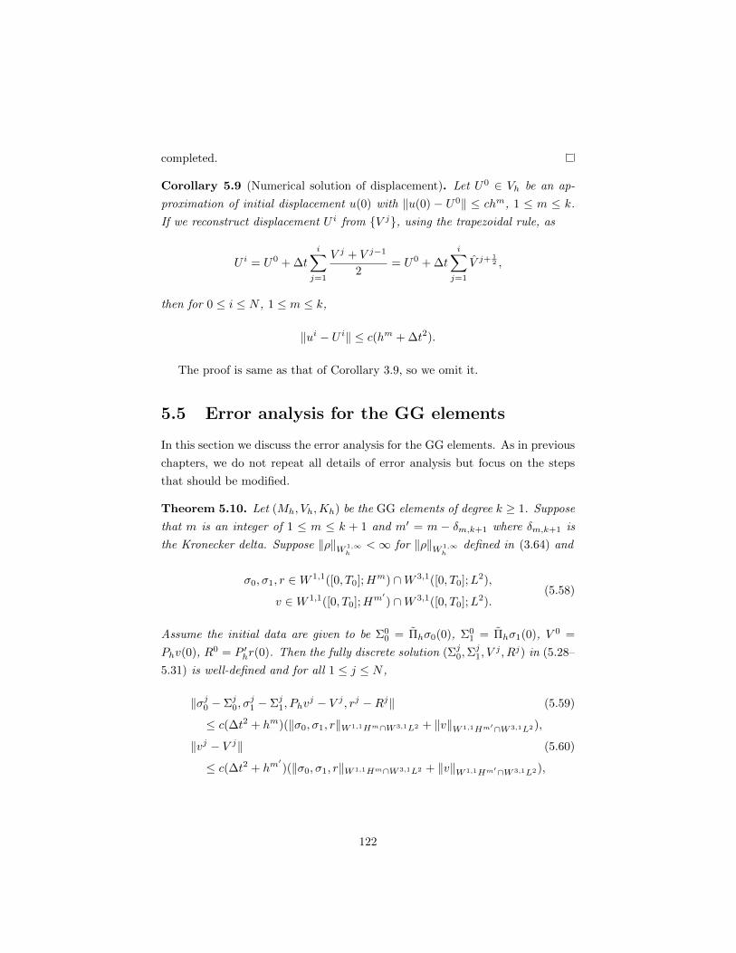
completed.
Corollary 5.9 (Numerical solution of displacement). Let U0 ∈ Vh be an ap-
proximation of initial displacement u(0) with ‖u(0) − U0‖ ≤ chm, 1 ≤ m ≤ k.
If we reconstruct displacement U i from V j, using the trapezoidal rule, as
U i = U0 + ∆t
i∑j=1
V j + V j−1
2= U0 + ∆t
i∑j=1
V j+12 ,
then for 0 ≤ i ≤ N , 1 ≤ m ≤ k,
‖ui − U i‖ ≤ c(hm + ∆t2).
The proof is same as that of Corollary 3.9, so we omit it.
5.5 Error analysis for the GG elements
In this section we discuss the error analysis for the GG elements. As in previous
chapters, we do not repeat all details of error analysis but focus on the steps
that should be modified.
Theorem 5.10. Let (Mh, Vh,Kh) be the GG elements of degree k ≥ 1. Suppose
that m is an integer of 1 ≤ m ≤ k + 1 and m′ = m − δm,k+1 where δm,k+1 is
the Kronecker delta. Suppose ‖ρ‖W 1,∞h
<∞ for ‖ρ‖W 1,∞h
defined in (3.64) and
σ0, σ1, r ∈W 1,1([0, T0];Hm) ∩W 3,1([0, T0];L2),
v ∈W 1,1([0, T0];Hm′) ∩W 3,1([0, T0];L2).(5.58)
Assume the initial data are given to be Σ00 = Πhσ0(0), Σ0
1 = Πhσ1(0), V 0 =
Phv(0), R0 = P ′hr(0). Then the fully discrete solution (Σj0,Σj1, V
j , Rj) in (5.28–
5.31) is well-defined and for all 1 ≤ j ≤ N ,
‖σj0 − Σj0, σj1 − Σj1, Phv
j − V j , rj −Rj‖ (5.59)
≤ c(∆t2 + hm)(‖σ0, σ1, r‖W 1,1Hm∩W 3,1L2 + ‖v‖W 1,1Hm′∩W 3,1L2),
‖vj − V j‖ (5.60)
≤ c(∆t2 + hm′)(‖σ0, σ1, r‖W 1,1Hm∩W 3,1L2 + ‖v‖W 1,1Hm′∩W 3,1L2),
122

where c depends on A0, A′0, A1, ρ0, and ‖ρ‖W 1,∞h
but is independent of h and
∆t. The constants c in (5.59–5.60) are uniformly bounded as A′0 decays.
Well-definedness of fully discrete solutions is same as the proof of Theo-
rem 5.7, so we only discuss a priori error estimates. We decompose the errors
(Ejσ0, Ejσ1
, Ejv, Ejr) into the projection errors (eP,jσ0
, eP,jσ1, eP,jv , eP,jr ) and the ap-
proximation errors (θjσ0, θjσ1
, θjv, θjr) as in (5.34–5.36).
Theorem 5.11. There exists a constant c > 0 independent h so that the fol-
lowing inequalities hold.
‖ePσi‖ ≤ chm‖σi‖m, 1 ≤ m ≤ k + 1, i = 0, 1,
‖ePv ‖ ≤ chm‖v‖m, 0 ≤ m ≤ k,
‖ePr ‖ ≤ chm‖r‖m, 0 ≤ m ≤ k + 1.
Furthermore, similar inequalities hold for the time derivatives of σ0, σ1, v, and
r, respectively, as in Theorem 5.5.
We omit its proof because it is same as the proof of Theorem 5.5.
For Theorem 5.10, we only need to consider a priori estimates of the approx-
imation errors (θjσ0, θjσ1
, θjv, θjr) by the triangle inequality.
Theorem 5.12. Suppose the assumptions in Theorem 5.10 hold and θiσ0, θjσ1
,
θiv, θir are defined as in (5.34–5.36). Then there exists a constant c > 0 depending
on A0, A′0, A1, ρ0, ‖ρ‖W 1,∞h
but is independent of h and ∆t so that
‖θiσ0, θiσ1
, θiv, θir‖
≤ c(∆t2 + hm)(‖σ0, σ1, r‖W 1,1Hm∩W 3,1L2 + ‖v‖W 1,1Hm′∩W 3,1L2), (5.61)
for 0 ≤ i ≤ N , 1 ≤ m ≤ k + 1.
Proof. For a priori error estimates, we follow same argument in the proof of
Theorem 5.7 and obtain (5.45).
To prove (5.61) for ‖θiσ0, θiσ1
, θiv‖, let ρc be the orthogonal L2 projection of ρ
into the space of piecewise constant functions associated to Th. Then we define
ωj+1/29 = (ρ− ρc)∂teP,j+1/2
v . Note that ρc∂teP,j+1/2v ⊥ Vh from the definition of
∂teP,j+1/2v and
(ωj+ 1
29 , θ
j+ 12
v ) = (ρ∂tvP,j+ 1
2 , θj+ 1
2v ) = ((ρ− ρc)∂te
P,j+ 12
v , θj+ 1
2v ) = (ω
j+ 12
9 , θj+ 1
2v ).
123

Therefore we have an inequality analogous to (5.46) as follows.
(‖θj+1σ0‖2A0
+ ‖θj+1σ1‖2A1
+ ‖θj+1v ‖2ρ)
12
≤ (‖θjσ0‖2A0
+ ‖θjσ1‖2A1
+ ‖θjv‖2ρ)12 + c∆t
(8∑l=1
‖ωj+12
l ‖+ ‖ωj+12
9 ‖
).
Repeating the steps in (5.46) and (5.47), for the proof of (5.61) for ‖θiσ0, θiσ1
, θiv‖,we only need to show
c∆t
i−1∑j=0
(8∑l=1
‖ωj+12
l ‖+ ‖ωj+12
9 ‖
)≤ c(∆t2 + hm), 1 ≤ m ≤ k + 1.
For the estimates of ωj+1/2l , l = 1, · · · , 8, we use (5.49–5.56) and note that the
integer m ranges 1 ≤ m ≤ k + 1 for the GG elements. For ωj+1/29 ,
∆t‖ωj+12
9 ‖ = ∆t‖(ρ− ρc)∂teP,jv ‖ =
∥∥∥∥∥∫ tj+1
tj
(ρ− ρc)(vPh − v) ds
∥∥∥∥∥≤ chm+1‖ρ‖W 1,∞
h
∫ tj+1
tj
‖v‖mds, 1 ≤ m ≤ k.
For the proof of (5.61) for ‖θir‖, we repeat the argument for ‖θir‖ in the proof
of Theorem 5.8. Details are omitted.
We also claim that a simple postprocessing can be used to find a better
numerical solution of u as we have done in previous chapters. Its proof is same
as the proof of Theorem 3.13, so we only state it below without a proof.
For Vh in the GG elements, let V ∗h be the space of (possibly discontinuous)
piecewise polynomials of one degree higher than Vh, and Vh be the orthogonal
complement of Vh in V ∗h . The orthogonal L2 projections onto V ∗h and Vh are
denoted by P ∗h and Ph.
Theorem 5.13. Suppose that Theorem 5.10 holds with m = k + 1 and also
‖v‖W 1,1Hk+1 <∞. Let U i be a numerical solution of displacement in Corollary
5.9 with an assumption that ‖Phu(0)− U0‖ ≤ chk+1. We define U∗,i ∈ V ∗h by
(gradh U∗,i, gradh w) = (A1Σi1 +Ri, gradh w), w ∈ Vh, (5.62)
(U∗,i, w) = (U i, w), w ∈ Vh, (5.63)
124

for each 0 ≤ i ≤ N where gradh is the piecewise gradient operator adapted to the
triangulation Th. Then U∗,i is well-defined and there exists c > 0 independent
of h and ∆t such that
‖ui − U∗,i‖ ≤ c(∆t2 + hk+1)‖σ0, σ1, v, r‖W 1,1Hk+1∩W 3,1L2 . (5.64)
5.6 Numerical results
In this section, we present numerical results. We use Ω = [0, 1] × [0, 1] and
the AFW elements of degree k = 2 in all our numerical computations. We
assume that the medium is homogeneous with density ρ = 1, and compliance
tensors A0, A′0, A1 are given as in (2.7) with parameters µ0, λ0, µ′0, λ′0, µ1,
λ1. For simplicity, we put µ0 = λ0 = 1, µ′0 = λ′0 = 5, and µ1 = λ1 = 10 in all
experiments.
For each spatial mesh size h, we take ∆t = h for time step ∆t, so the expected
order of convergence is 2 from our error bound O(h2+∆t2). We present L2 errors
of σ0, σ1, v, and r at time T0 = 1, with mesh sizes h = 1/4, 1/8, 1/16, 1/32, 1/64,
and compute the order of convergences.
Finally, as in the previous chapters, all codes are implemented using the
Dolfin Python module [1] of FEniCS project [2, 38].
Example 5.14. Let the displacement field be
u(t, x, y) =
((1− x)x2 sin(πy) cos t
(1 + t) sin(πx) sin(πy)
), (5.65)
and σ0(0) = 0. Then one can find v, σ0, σ1, and f using (5.1). For this exact
solution, we compute a numerical solution with inhomogeneous displacement
Table 5.1: Order of convergence for the exact solution with the displacement asin (5.65) and σ0(0) = 0 (µ0 = λ0 = 1, µ′0 = λ′0 = 5, µ1 = λ1 = 10, h = ∆t andT0 = 1).
1h
‖σ0 − σ0,h‖ ‖σ1 − σ1,h‖ ‖v − vh‖ ‖r − rh‖error order error order error order error order
4 2.37e-01 – 1.08e+00 – 1.96e-02 – 5.77e-02 –
8 3.15e-02 2.91 1.83e-01 2.55 4.88e-03 2.01 1.46e-02 1.99
16 4.81e-03 2.71 3.82e-02 2.26 1.22e-03 2.00 3.64e-03 2.00
32 9.11e-04 2.40 8.93e-03 2.10 3.05e-04 2.00 9.09e-04 2.00
64 2.05e-04 2.15 2.18e-03 2.03 7.62e-05 2.00 2.27e-04 2.00
125

Table 5.2: Order of convergence for the exact solution with the displacement asin (5.66) and σ0(0) = 0 (µ0 = λ0 = 1, µ′0 = λ′0 = 5, µ1 = λ1 = 10, h = ∆t andT0 = 1).
1h
‖σ0 − σ0,h‖ ‖σ1 − σ1,h‖ ‖v − vh‖ ‖r − rh‖error order error order error order error order
4 1.79e-02 – 2.28e-01 – 8.41e-03 – 9.07e-03 –
8 4.44e-03 2.01 5.67e-02 2.01 2.09e-03 2.01 2.27e-03 2.00
16 1.11e-03 2.00 1.41e-02 2.00 5.17e-04 2.01 5.67e-04 2.00
32 2.76e-04 2.00 3.53e-03 2.00 1.29e-04 2.00 1.42e-04 2.00
64 6.90e-05 2.00 8.83e-04 2.00 3.22e-05 2.00 3.54e-05 2.00
boundary conditions using the weak formulation (5.6–5.9). The numerical result
for (5.65) is in Table 5.1.
Example 5.15. As an example with inhomogeneous displacement boundary
conditions, we let the displacement field be
u(t, x, y) =
(e−y cos t sinx
et+x
), (5.66)
and let σ0(0) = 0. Then one can compute v, σ0, σ1, and f using (5.1). We
compute a numerical solution with inhomogeneous displacement boundary con-
ditions using the weak formulation (5.6–5.9). The numerical results for (5.66)
are shown in Table 5.2.
Example 5.16. For a nonsmooth solution, let
u(t, x, y) =
((1 + t2)x
73 y
y73 cos t
), (5.67)
Table 5.3: Order of convergence for the exact solution with displacement as in(5.67) and σ0(0) = 0 (µ0 = λ0 = 1, µ′0 = λ′0 = 5, µ1 = λ1 = 10, h = ∆t andT0 = 1).
1h
‖σ0 − σ0,h‖ ‖σ1 − σ1,h‖ ‖v − vh‖ ‖r − rh‖error order error order error order error order
4 3.61e-01 – 2.27e-01 – 1.07e-02 – 4.27e-03 –
8 1.06e-01 1.76 6.44e-02 1.82 2.63e-03 2.02 1.05e-03 2.03
16 3.06e-02 1.80 1.81e-02 1.83 6.52e-04 2.01 2.60e-04 2.01
32 8.69e-03 1.81 5.07e-03 1.84 1.62e-04 2.01 6.46e-05 2.01
64 2.45e-03 1.82 1.42e-03 1.84 4.04e-05 2.00 1.61e-05 2.00
126

and σ0(0) = 0. The corresponding σ0, σ1 are((70t− 350)yx
43 + 35
78y43 (5 cos t− sin t) 10(−5 + t)x
73
10(−5 + t)x73
703 (t− 5)yx
43 + 35
26y43 (5 cos t− sin t)
),
10
(7y((1 + t2)x
43 + y
13 cos t) (1 + t2)x
73
(1 + t2)x73
73y((1 + t2)x
43 + 3y
13 cos t)
),
respectively. From the fractional order 4/3 of polynomial terms in σ0 and σ1,
they belong to H5/6−δ in space for any δ > 0.
As in the previous example, we compute a numerical solution with inhomoge-
neous displacement boundary condition using (5.8–5.9). The numerical results
for (5.67) are shown in Table 5.3. The orders of convergence of σ0, σ1 approach
11/6 ≈ 1.833 as we expected in our error analysis but the order of convergence
of v is 2. It is consistent to the results we have seen for the examples of elasto-
dynamics and the equations of the Kelvin–Voigt model in the previous chapters,
so we again get a motivation to study a better estimate for the v error.
127

Chapter 6
Numerical simulations
In this chapter we present numerical simulations which are more closely involved
in physical situations using the numerical schemes that we developed in previous
chapters. In section 6.1, we show wave propagation in homogeneous isotropic,
heterogeneous isotropic, and anisotropic elastic media. In section 6.2, we show
the creep test of viscoelastic materials and one seismology model problem of
wave propagation in viscoelastic media.
6.1 Elastodynamics
In this section, we present three numerical simulations. In the first simulation,
we will see the difference of two different types of wave propagation, P and S
waves, in homogeneous isotropic medium. In the second simulation, we consider
two isotropic heterogeneous media and will see that different parameters of elas-
tic media affect differently to P and S waves. In the last one, we consider wave
propagation in two anisotropic materials and show that a radially symmetric
initial data becomes asymmetric waves.
6.1.1 Wave propagation in homogeneous isotropic elastic
media
In Figure 6.1, we see a series of screen-shots of wave propagation in an isotropic
homogeneous linear elastic medium. For initial data, the initial displacement is
vanishing (hence initial stress is vanishing) and the initial velocity is given as a
bump function of horizontal direction. The magnitude of wave is described as
128

height in Figure 6.1. The splitting of P and S waves is one of the features of
Figure 6.1: Magnitude of elastic waves in homogeneous isotropic elasticmedium.
elastic wave propagation. It is known that P wave is faster than S wave, but
S wave is more destructive. In the above figures, we observe these features of
P and S waves. We can see that P wave mostly propagates horizontally with
faster speed and small magnitude, but S wave propagates vertically with slower
speed and big magnitude.
6.1.2 Wave propagation in isotropic heterogeneous elastic
media
We compare wave propagation in two different heterogeneous media with same
initial data. In these simulations, we can see different parameters of elastic
medium influence differently to propagation of P and S waves.
The domain is [−6, 6] × [−6, 6] and the two media are heterogeneous with
different parameters on the left and right of the vertical line x = −1.2. For
129

convenience, we call the two subdomains, splited by x = −1.2, as left and
right domains. In Figure 6.2, we see the wave propagation is not completely
symmetric with respect to x = −1.2, but two crescent shape waves propagate
symmetrically. It is because S wave propagation is not affected by the difference
of material parameter, but P wave is affected and has increased propagation
speed.
On the contrary, we can see both S and P waves propagates faster on right
domain in Figure 6.3. Since there are reflections and refractions of waves, the
wave propagation becomes more complicated in time and is not simply de-
scribed.
6.1.3 Wave propagation in anisotropic media
Wave propagation in anisotropic materials is much more complicated than the
one in isotropic materials. The elastic waves in anisotropic materials are not
simply classified into P and S waves, so it is extremely difficult to classify waves
and establish principles on wave propagation even in linear elastodynamics. This
is a broad research area which still needs many works to be done in the future.
Therefore we do not discuss theoretical parts of this topic but present wave
propagation examples on the media which may somewhat represent features of
components of the compliance tensor.
For initial data, we always give a radially symmetric initial velocity and
vanishing stress, so vanishing displacement as well. In isotropic media, the
wave propagation with this initial data is radially symmetric as we see in Figure
6.4. However, we see that wave propagation in anisotropic media may become
strongly asymmetric up to the compliance tensor, which is a symmetric 3 × 3
matrix A satisfying ε11
ε12
ε22
= A
σ11
σ12
σ22
.
For the materials that we used in our numerical computations, compliance ten-
sors are given by
Orthotropic 1 : c
4 0 −1/2
0 4 0
−1/2 0 2
, Orthotropic 2 : c
4 0 −1
0 4 0
−1 0 2
,
130

Figure 6.2: Magnitude of waves in heterogeneous medium 1. For the medium1, the Lame coefficient λ is 90 if x ≤ −1.2 and is 10 if x > −1.2. Another Lamecoefficient µ is 10, and the mass density ρ is 5 on the whole domain.
where c = 1.0e − 2. These are examples of orthotropic materials which means
that the material has two or three mutually orthogonal twofold axes of rotational
symmetry. For more details on orthotropic materials, see [43]
In all examples, ρ = 10. For the domain of numerical computations, [−5, 5]×[−5, 5] is used with the triangulation that 100 meshes in horizontal and vertical
directions. The AFW elements of degree 2 is used for spatial discretization
131

Figure 6.3: Magnitude of waves in heterogeneous medium 2. For the medium2, the Lame coefficients λ and µ are both 10 on the whole domain but the massdensity is 5 if x ≤ −1.2 and is 45 if x > −1.2.
and the Crank–Nicolson scheme is used for time discretization with time step
∆t = 0.01. In all figures, the red–blue color range corresponds to the magnitude
of displacement.
In Figures 6.4–6.6, we compare wave propagation in an isotropic medium,
and two orthotropic media. The media Ortho. 1 and Ortho. 2 have compliance
tensors which are given as above.
132

Figure 6.4: Isotropic Figure 6.5: Ortho. 1 Figure 6.6: Ortho. 2
133

6.2 Viscoelasticity of materials
In this section, we show numerical experiments which are more involved in
physical implications. In 6.2.1, we compare creep compliances of the viscoelastic
models.
6.2.1 Creep compliance
We use our numerical schemes to test creep compliance of viscoelastic materials.
As a model problem, we consider a rectangular object on [−1, 1] × [0, 1]. We
assume that the top is clamped, i.e., vanishing displacement boundary condi-
tions are given. For the other sides, the left and right are traction-free and the
bottom is exerted by a given normal force(0
10e−10x2
)
only from t = 2 to t = 10.
In our numerical computations, we used 16×32 mesh refinements, the AFW
elements of degree 1, and ∆t = 0.1 for time stepping. The mass density ρ is 1
in all simulations. The materials parameters are
Zener : µ0 = 500, µ1 = µ2 = 10, λ0 = 500, λ1 = λ2 = 10,
Kelvin–Voigt : µ0 = µ1 = 10, λ0 = λ1 = 100,
Maxwell : µ0 = 1000, µ1 = 100, λ0 = 1000, λ1 = 100.
Note that these parameters are not involved in specific physical motivations and
are only based on purely numerical experiments for visualization.
In Figure 6.7 we compare vertical displacements at (0, 0) in time of the
three materials. In this figure, we can see that the Zener and Kelvin–Voigt
models show similar behaviors. From the physical viewpoint, the shape begins
deforming under the exerted force at t = 2 but the deformation process is not
instantaneous. When the exerted force is removed at t = 10, the shape recovers
to the original shape but this recovering is not instantaneous either. We can see
that the Maxwell model shows a very different, fluid-like, behavior. The shape
deformation is proportional to the exerted time and it does not recover after
the exerted force is removed.
134

6.2.2 Attenuation of reflected waves
We consider a simple model problem for reflected waves. We compare reflected
waves for two media. The first medium, say Medium I, consists of purely elastic
materials and the second medium, Medium II, has an intermediate layer which
is viscoelastic. In Figure 6.8, regions of elastic and viscoelastic materials are
described. We call the three layers as Layer 1, 2, and 3.
For implementation, we use the Zener model with A′0 which is vanishing
on regions that the medium is elastic. The domain is [−15, 15] × [−15, 0] with
0 2 4 6 8 10 12 14 16 18 20−0.2
−0.1
0
0.1
0.2
0.3
0.4
0.5
Zener
Kelvin−Voigt
Maxwell
Figure 6.7: Comparison of creep compliances of the Zener, Kelvin–Voigt, andMaxwell models. (∆t = 0.1)
elasticelastic/viscoelastic
elastic with high mass density
Figure 6.8: Regions of elastic and viscoelastic materials.
135

180× 60 structured triangular meshes. The coordinates of two internal border
lines of layers are y = −1.5, y = −3.0, respectively. We used the AFW elements
of degree 1 and the time step interval is ∆t = 0.01. The material parameters in
the layers for Medium I and II are as follows.
Medium I
Layer 1 : µ0 = µ2 = λ0 = λ2 = 10, ρ = 1
Layer 2 : µ0 = µ2 = λ0 = λ2 = 10, ρ = 1
Layer 3 : µ0 = µ2 = λ0 = λ2 = 10, ρ = 5.
Medium II
Layer 1 : µ0 = µ2 = λ0 = λ2 = 10, ρ = 1
Layer 2 : µ0 = µ2 = λ0 = λ2 = 10, µ1 = λ1 = 500, ρ = 1
Layer 3 : µ0 = µ2 = λ0 = λ2 = 10, ρ = 5.
0 0.5 1 1.5 2 2.5 30
0.5
1
1.5
2
2.5x 10
−5
ElasticViscoelastic
Figure 6.9: Magnitude of reflected waves for the media of elastic and viscoelasticintermediate layers.
136

In Figure 6.9, we recorded the magnitude of displacement at (0.0) for Medium
I and II. The red dashed line, denoting the magnitude of the reflected waves
for Medium II, has lower peak than the one for Medium I. Although this model
is a schematic simplified one and the material parameters are not based on
physical motivations, we expect that this attenuation phenomenon of reflected
waves can be used for constructing more realistic models when it is combined
with experimental data in practical situations. However, a further study of this
modeling problem is beyond the scope of this dissertation.
137

Bibliography
[1] Website, https://launchpad.net/dolfin.
[2] Website, http://fenicsproject.org/.
[3] M. Amara and J. M. Thomas, Equilibrium finite elements for the linear
elastic problem, Numer. Math. 33 (1979), no. 4, 367–383. MR 553347
(81b:65096)
[4] Douglas N. Arnold and Gerard Awanou, Rectangular mixed finite elements
for elasticity, Math. Models Methods Appl. Sci. 15 (2005), no. 9, 1417–
1429. MR 2166210 (2006f:65112)
[5] Douglas N. Arnold, Gerard Awanou, and Ragnar Winther, Finite elements
for symmetric tensors in three dimensions, Math. Comp. 77 (2008), no. 263,
1229–1251. MR 2398766 (2009b:65291)
[6] Douglas N. Arnold and F. Brezzi, Mixed and nonconforming finite element
methods: implementation, postprocessing and error estimates, RAIRO
Model. Math. Anal. Numer. 19 (1985), no. 1, 7–32. MR 813687 (87g:65126)
[7] Douglas N. Arnold, Franco Brezzi, and Jr. Jim Douglas, PEERS: a new
mixed finite element for plane elasticity, Japan J. Appl. Math. 1 (1984),
347–367. MR 2601614
[8] Douglas N. Arnold, Jr. Jim Douglas, and Chaitan P. Gupta, A family
of higher order mixed finite element methods for plane elasticity, Numer.
Math. 45 (1984), no. 1, 1–22. MR 761879 (86a:65112)
[9] Douglas N. Arnold, Richard S. Falk, and Ragnar Winther, Finite element
exterior calculus, homological techniques, and applications, Acta Numer.
15 (2006), 1–155. MR 2269741 (2007j:58002)
138

[10] , Mixed finite element methods for linear elasticity with weakly im-
posed symmetry, Math. Comp. 76 (2007), no. 260, 1699–1723 (electronic).
MR 2336264 (2008k:74057)
[11] Douglas N. Arnold and Ragnar Winther, Mixed finite elements for elastic-
ity, Numer. Math. 92 (2002), no. 3, 401–419. MR 1930384 (2003i:65103)
[12] Uri M. Ascher, Numerical methods for evolutionary differential equa-
tions, Computational Science & Engineering, vol. 5, Society for Industrial
and Applied Mathematics (SIAM), Philadelphia, PA, 2008. MR 2420042
(2009f:65001)
[13] Gerard Awanou, Rectangular mixed elements for elasticity with weakly im-
posed symmetry condition, Advances in Computational Mathematics, 1–17,
10.1007/s10444-011-9240-1.
[14] R L Bagley and P. J. Torvik, A theoretical basis for the application of
fractional calculus to viscoelasticity, Journal of Rheology 27 (1983), no. 3,
201–210.
[15] E. Becache, P. Joly, and C. Tsogka, A new family of mixed finite elements
for the linear elastodynamic problem, SIAM J. Numer. Anal. 39 (2002),
no. 6, 2109–2132 (electronic). MR 1897952 (2003d:65089)
[16] Eliane Becache, Abdelaaziz Ezziani, and Patrick Joly, A mixed finite ele-
ment approach for viscoelastic wave propagation, Comput. Geosci. 8 (2004),
no. 3, 255–299. MR 2121266 (2005k:74073)
[17] Daniele Boffi, Franco Brezzi, Leszek F. Demkowicz, Ricardo G. Duran,
Richard S. Falk, and Michel Fortin, Mixed finite elements, compatibility
conditions, and applications, Lecture Notes in Mathematics, vol. 1939,
Springer-Verlag, Berlin, 2008, Lectures given at the C.I.M.E. Summer
School held in Cetraro, June 26–July 1, 2006, Edited by Boffi and Lucia
Gastaldi. MR 2459075 (2010h:65219)
[18] Susanne C. Brenner and L. Ridgway Scott, The mathematical theory of
finite element methods, Third ed., Springer, 2008. MR 515228 (80k:35056)
[19] F. Brezzi and M. Fortin, Mixed and hybrid finite element methods,
Springer Series in computational Mathematics, vol. 15, Springer, 1992. MR
MR2233925 (2008i:35211)
139

[20] C. Carstensen, D. Gunther, J. Reininghaus, and J. Thiele, The Arnold-
Winther mixed FEM in linear elasticity. I. Implementation and numerical
verification, Comput. Methods Appl. Mech. Engrg. 197 (2008), no. 33-40,
3014–3023. MR 2427098 (2009h:74093)
[21] Thierry Cazenave and Alain Haraux, An introduction to semilinear evolu-
tion equations, Oxford Lecture Series in Mathematics and its Applications,
vol. 13, The Clarendon Press Oxford University Press, New York, 1998,
Translated from the 1990 French original by Yvan Martel and revised by
the authors. MR 1691574 (2000e:35003)
[22] Philippe G. Ciarlet, Mathematical elasticity. Vol. I, Studies in Mathematics
and its Applications, vol. 20, North-Holland Publishing Co., Amsterdam,
1988, Three-dimensional elasticity. MR 936420 (89e:73001)
[23] Ph. Clement, Approximation by finite element functions using local regular-
ization, Rev. Francaise Automat. Informat. Recherche Operationnelle Ser.
Rouge 9 (1975), no. R-2, 77–84. MR 0400739 (53 #4569)
[24] Bernardo Cockburn, Jayadeep Gopalakrishnan, and Johnny Guzman, A
new elasticity element made for enforcing weak stress symmetry, Math.
Comp. 79 (2010), no. 271, 1331–1349. MR 2629995
[25] Earl A. Coddington and Norman Levinson, Theory of ordinary differential
equations, McGraw-Hill Book Company, Inc., New York-Toronto-London,
1955. MR 0069338 (16,1022b)
[26] B. X. Fraeijs de Veubeke, Stress function approach, Proceedings of the
World Congress on Finite Element Methods in Structural Mechanics, vol. 5,
1975, pp. J.1 – J.51.
[27] Jr. Jim Douglas and Chaitan P. Gupta, Superconvergence for a mixed finite
element method for elastic wave propagation in a plane domain, Numer.
Math. 49 (1986), no. 2-3, 189–202. MR 848520 (88c:65095)
[28] G. Duvaut and J.-L. Lions, Inequalities in mechanics and physics, Springer-
Verlag, Berlin, 1976, Translated from the French by C. W. John,
Grundlehren der Mathematischen Wissenschaften, 219. MR 0521262 (58
#25191)
140

[29] Michael Eastwood, A complex from linear elasticity, The Proceedings of
the 19th Winter School “Geometry and Physics” (Srnı, 1999), no. 63, 2000,
pp. 23–29. MR 1758075 (2001j:58033)
[30] Richard S. Falk, Finite elements for linear elasticity, Mixed Finite Ele-
ments: Compatibility Conditions (D. Boffi and L. Gastaldi, eds.), vol. 1939,
Springer, 2008.
[31] Tunc Geveci, On the application of mixed finite element methods to the wave
equations, RAIRO Model. Math. Anal. Numer. 22 (1988), no. 2, 243–250.
MR 945124 (89i:65116)
[32] J. Gopalakrishnan and J. Guzman, A second elasticity element using the
matrix bubble, IMA J. Numer. Anal. 32 (2012), no. 1, 352–372. MR 2875255
[33] M. E. Gurtin and Eli Sternberg, On the linear theory of viscoelasticity,
Arch. Rational Mech. Anal. 11 (1962), 291–356. MR 0147047 (26 #4565)
[34] Morton E. Gurtin, An introduction to continuum mechanics, Mathematics
in Science and Engineering, vol. 158, Academic Press Inc. [Harcourt Brace
Jovanovich Publishers], New York, 1981. MR 636255 (84c:73001)
[35] J. Guzman, A unified analysis of several mixed methods for elasticity with
weak stress symmetry, J. Sci. Comput. 44 (2010), no. 2, 156–169. MR
2659794 (2011h:74021)
[36] C. Johnson and B. Mercier, Some equilibrium finite element methods for
two-dimensional elasticity problems, Numer. Math. 30 (1978), no. 1, 103–
116. MR 0483904 (58 #3856)
[37] Marianna Karamanou, Simon Shaw, M. K. Warby, and J. R. Whiteman,
Models, algorithms and error estimation for computational viscoelasticity,
Comput. Methods Appl. Mech. Engrg. 194 (2005), no. 2-5, 245–265. MR
2105163 (2005g:74053)
[38] A. Logg, K.-A. Mardal, and G. N. Wells (eds.), Automated solution of
differential equations by the finite element method, Lecture Notes in Com-
putational Science and Engineering, vol. 84, Springer, 2012.
[39] Ch. G. Makridakis, On mixed finite element methods for linear elastody-
namics, Numer. Math. 61 (1992), no. 2, 235–260. MR 1147578 (92j:65142)
141

[40] Mary E. Morley, A family of mixed finite elements for linear elasticity,
Numer. Math. 55 (1989), no. 6, 633–666. MR 1005064 (90f:73006)
[41] J. Pitkaranta and R. Stenberg, Analysis of some mixed finite element meth-
ods for plane elasticity equations, Math. Comp. 41 (1983), no. 164, 399–423.
MR 717693 (85b:65099)
[42] P.-A. Raviart and J. M. Thomas, A mixed finite element method for
2nd order elliptic problems, Mathematical aspects of finite element meth-
ods (Proc. Conf., Consiglio Naz. delle Ricerche (C.N.R.), Rome, 1975),
Springer, Berlin, 1977, pp. 292–315. Lecture Notes in Math., Vol. 606. MR
0483555 (58 #3547)
[43] J. N. Reddy, An introduction to nonlinear finite element analysis, Oxford
University Press, Oxford, 2004. MR 2062304 (2005c:65001)
[44] M. Rognes and R. Winther, Mixed finite element methods for linear vis-
coelasticity using weak symmetry, Math. Models Methods Appl. Sci. 20
(2010), no. 6, 955–985.
[45] Walter Rudin, Functional analysis, second ed., International Series in Pure
and Applied Mathematics, McGraw-Hill Inc., New York, 1991. MR 1157815
(92k:46001)
[46] Rolf Stenberg, On the construction of optimal mixed finite element methods
for the linear elasticity problem, Numer. Math. 48 (1986), no. 4, 447–462.
MR 834332 (87i:73062)
[47] , A family of mixed finite elements for the elasticity problem, Numer.
Math. 53 (1988), no. 5, 513–538. MR 954768 (89h:65192)
[48] Nicholas W. Tschoegl, The phenomenological theory of linear viscoelas-
tic behavior, Springer-Verlag, Berlin, 1989, An introduction. MR 999136
(90f:73033)
[49] Mary Fanett Wheeler, A priori L2 error estimates for Galerkin approxi-
mations to parabolic partial differential equations, SIAM J. Numer. Anal.
10 (1973), 723–759. MR 0351124 (50 #3613)
[50] Kosaku Yosida, Functional analysis, 6th ed., Springer Classics in Mathe-
matics, Springer-Verlag, 1980.
142