mixed integer programming models for non-separable ...jvielma/presentations/pwl_pitt_08.pdf ·...

University of Pittsburgh, 2008 – Pittsburgh, PA

Mixed Integer Programming Models for

Non-Separable Piecewise Linear Cost

Functions

Juan Pablo Vielma

H. Milton Stewart School of Industrial and Systems Engineering

Georgia Institute of Technology

Joint work with Shabbir Ahmed and George Nemhauser.

is a piecewise linear

function (PLF) and is any compact set.

Convex = Linear Programming. Non-Convex = NP Hard.

Specialized algorithms (Tomlin 1981, ..., de Farias et al.

2008 ) or Mixed Integer Programming Models (12+ papers). /26

Piecewise Linear Optimization

2

min f0(x)

s.t.

fi(x) ≤0 ∀i ∈ I

x ∈X ⊂ Rn

/26

Mixed Integer Models for PLFs

Existing studies are for separable functions:

Contributions (Vielma et al. 2008a,b):

First models with a logarithmic # of binary variables.

Theoretical and computational comparison:

multivariate (non-separable) and lower

semicontinuous functions in a unifying framework.3

/26

Outline

Applications of Piecewise Linear Functions.

Modeling Piecewise Linear Functions.

Logarithmic Formulations.

Comparison of Formulations.

Extension to Lower Semicontinuous Functions.

Final Remarks.

4

/26

Applications of Piecewise Linear Functions

Economies of Scale: Concave

Single and multi-commodity network flow.

Applications in telecommunications, transportation,

and logistics.

(Balakrishnan and Graves 1989, ..., Croxton, et al. 2007).5

0 1 3 50

2

3.5

4

/26


Fixed Charges and Discounts

1.Fixed Costs in Logistics.

2.Discounts (e.g. Auctions: Sandholm,

et al. 2006, CombineNet).

3.Discounts in fixed charges (Lowe

1984).6

x

y

0

2

3

0 1 20

1

2

3

4

1. 2. 3.

0 1 30

1

2

3

Gas Network Optimization

(Martin et al. 2006)./26


Non-Linear and PDE Constraints

7

A∂ρ

∂t+ ρ0

∂q

∂x= 0,

∂p

∂x= −λ

|v|v

2Dρ .

Pipe

Demand Points

Pipes/Valves/

Compressors

Connections

Source

/26


Numerically Exact Global Optimization

Process engineering (Bergamini et al. 2005,

2008, Computers and Chemical Eng.)

Wetland restoration (Stralberg et al. 2009).8

/26


Numerically Exact Global Optimization

Process engineering (Bergamini et al. 2005,

2008, Computers and Chemical Eng.)

Wetland restoration (Stralberg et al. 2009).8

0.5 1.0 1.5 2.0 2.5 3.0

0.2

0.4

0.6

0.8

1.0

0 1 2 4 5

f(4) = 5

0

f(0) = 10

f(1) = 32

f(2) = 40

f(5) = 15

/26

Modeling Piecewise Linear Functions

Piecewise Linear Functions: Definition

9

Definition 1. Piecewise Linear f : D ⊂Rn →R:

f(x) :={mP x+ cP x∈ P ∀P ∈P.

for finite family of polytopes P such that D =⋃

P∈PP

f(x,y)

y

x ∈ P

/26


Piecewise Linear Functions: Definition

9

Definition 1. Piecewise Linear f : D ⊂Rn →R:

f(x) :={mP x+ cP x∈ P ∀P ∈P.

for finite family of polytopes P such that D =⋃

P∈PP

/26


Modeling Function = Epigraph

Example: 10

0 1 2 4 5

f(4) = 5

0

f(0) = 10

f(1) = 32

f(2) = 40

f(5) = 15

(a) f .

0 1 2 4 5

5

0

10

32

40

15

(b) epi(f).

/26


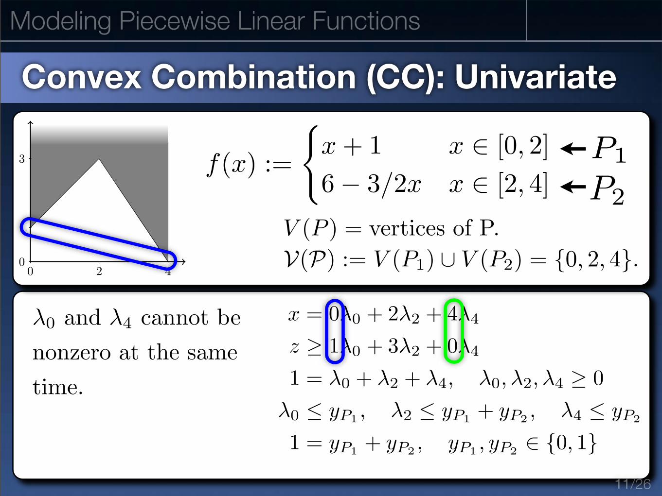
Convex Combination (CC): Univariate

11

0

1

3

2

0 2 4

λP1,

/26



11

0

1

3

=

0 2 4

1

3

0 2

∪

0

3

2 4

λP1,

/26



11

0

1

3

=

0 2 4

1

3

0 2

∪

0

3

2 4

x = 0λ0 + 2λ2 + 4λ4

z ≥ 1λ0 + 3λ2 + 0λ4

1 = λ0 + λ2 + λ4, λ0, λ2, λ4 ≥ 0

λ0 ≤ yP1, λ2 ≤ yP1

+ yP2, λ4 ≤ yP2

1 = yP1+ yP2

, yP1, yP2

∈ {0, 1}

λP1,

/26



11

0

1

3

=

0 2 4

1

3

0 2

∪

0

3

2 4

are SOS2

x = 0λ0 + 2λ2 + 4λ4

z ≥ 1λ0 + 3λ2 + 0λ4

1 = λ0 + λ2 + λ4, λ0, λ2, λ4 ≥ 0

λ0 ≤ yP1, λ2 ≤ yP1

+ yP2, λ4 ≤ yP2

1 = yP1+ yP2

, yP1, yP2

∈ {0, 1}

λP1,

Univariate (Dantzig, 1960) ... Multivariate (Lee and

Wilson (2001).

/26


Convex Combination (CC): Multivariate

12

∑v∈V(P)

λvv = x,∑

v∈V(P)

λv (mP v + cP )≤ z

λv ≥ 0 ∀v ∈ V(P) :=

⋃P∈P

V (P ),∑

v∈V(P)

λv = 1

λv ≤∑

{P∈P :v∈V (P )}

yP ∀v ∈ V(P),∑

P∈P

yP = 1, yP ∈ {0,1} ∀P ∈P


Wilson (2001).

/26



12

∑v∈V(P)

λvv = x,∑

v∈V(P)


λv ≥ 0 ∀v ∈ V(P) :=

⋃P∈P

V (P ),∑

v∈V(P)

λv = 1

λv ≤∑

{P∈P :v∈V (P )}

yP ∀v ∈ V(P),∑

P∈P

yP = 1, yP ∈ {0,1} ∀P ∈P


Wilson (2001).

/26



12

“Original

Constraints”

∑v∈V(P)

λvv = x,∑

v∈V(P)


λv ≥ 0 ∀v ∈ V(P) :=

⋃P∈P

V (P ),∑

v∈V(P)

λv = 1

λv ≤∑

{P∈P :v∈V (P )}

yP ∀v ∈ V(P),∑

P∈P

yP = 1, yP ∈ {0,1} ∀P ∈P


Wilson (2001).

/26



12

“Extra

Constraints”

∑v∈V(P)

λvv = x,∑

v∈V(P)


λv ≥ 0 ∀v ∈ V(P) :=

⋃P∈P

V (P ),∑

v∈V(P)

λv = 1

λv ≤∑

{P∈P :v∈V (P )}

yP ∀v ∈ V(P),∑

P∈P

yP = 1, yP ∈ {0,1} ∀P ∈P


Wilson (2001).

/26



SOS2 only for univariate

12

“Extra

Constraints”

Nonzero variables are associated to vertices of a

single polytope.

∑v∈V(P)

λvv = x,∑

v∈V(P)


λv ≥ 0 ∀v ∈ V(P) :=

⋃P∈P

V (P ),∑

v∈V(P)

λv = 1

λv ≤∑

{P∈P :v∈V (P )}

yP ∀v ∈ V(P),∑

P∈P

yP = 1, yP ∈ {0,1} ∀P ∈P


Wilson (2001).

/26



12

“Extra

Constraints”

/26


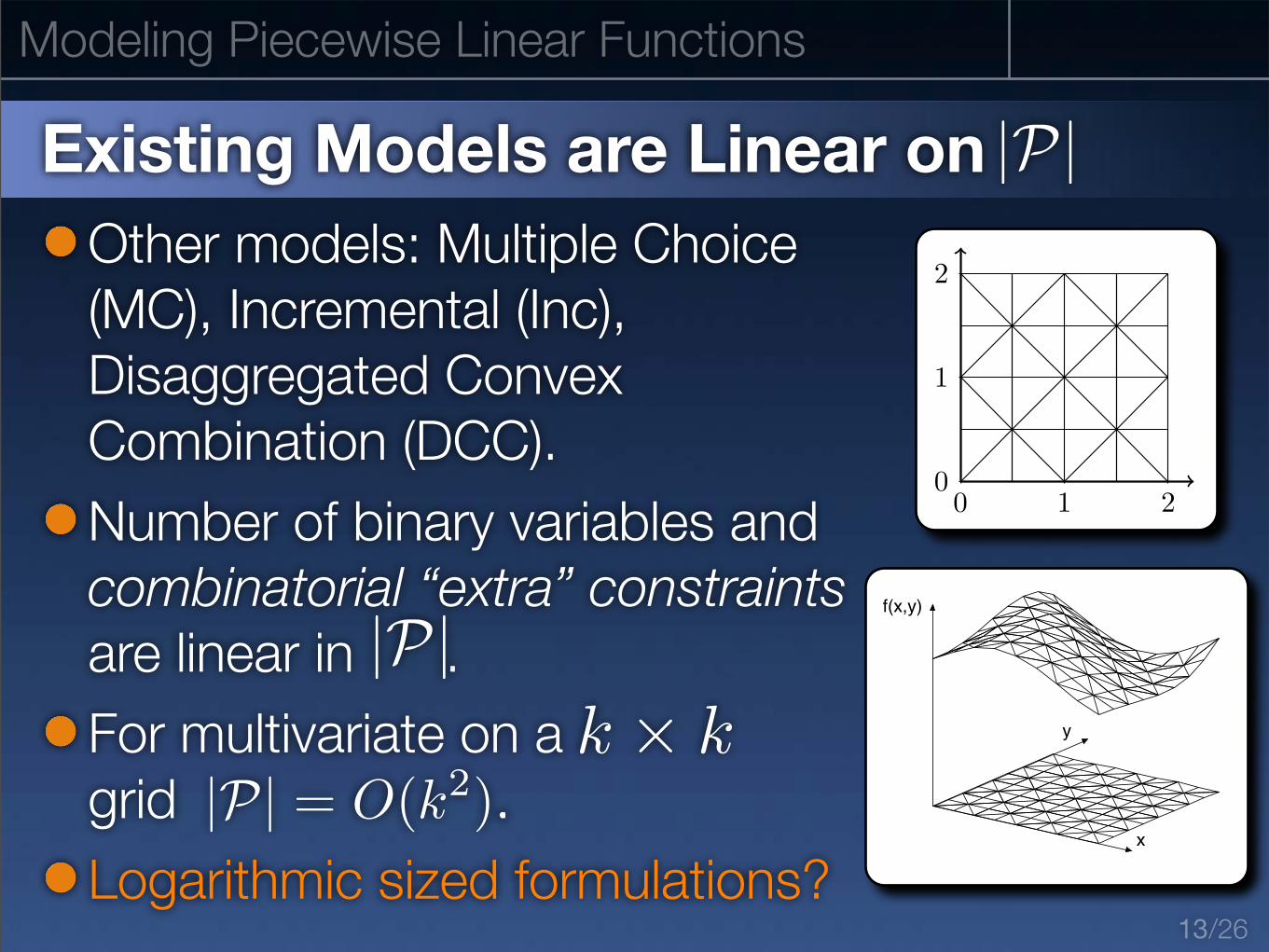
Existing Models are Linear on

Other models: Multiple Choice

(MC), Incremental (Inc),

Disaggregated Convex

Combination (DCC).

Number of binary variables and

combinatorial “extra” constraints

are linear in .

For multivariate on a

grid .

Logarithmic sized formulations?13

f(x,y)

y

x

0 1 20

1

2

SOS1-2 (Beale and Tomlin 1970):

SOS1: At most one variable is nonzero.

SOS2: Only 2 adjacent variables are nonzero.

! (0,1,1/2,0,0) ! (0,1,0,1/2,0)

, allowed sets .

SOS1:

SOS2:

CC:/26

Logarithmic Formulations

SOS1, SOS2 and CC constraints.

14

/26


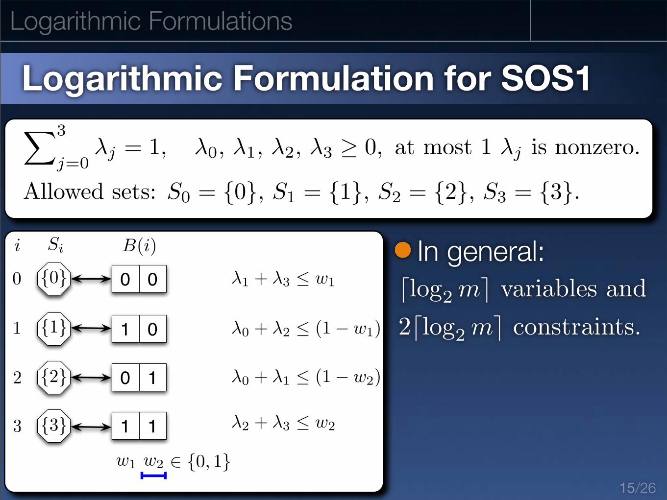
Logarithmic Formulation for SOS1

15

Injective function:

Variables:

Idea:

0 0

1 0

0 1

1 1

/26



15

B : {0, . . . ,m− 1}→ {0,1}⌈log2 m⌉

w ∈ {0,1}⌈log2 m⌉

0 0

1 0

0 1

1 1

/26



15

In general:

/26



16

0 0

1 0

0 1

1 1

Injective function:

Variables:

Idea:

/26



16

B : {0, . . . ,m− 1}→ {0,1}⌈log2 m⌉

w ∈ {0,1}⌈log2 m⌉

0 0

1 0

0 1

1 1

/26



16

Where is ?!λ2

0 0

1 0

0 1

1 1

/26



16

Where is ?!λ2

/26



16

0 0

1 0

1 1

0 1

Where is ?!

In general:

Gray Code.

λ2

/26



16

0 0

1 0

1 1

0 1

B(i) and B(i+1)

differ in one component

/26


Independent Branching: Dichotomies

17

λ0

λ1

λ2

λ3

λ4

λ0

λ1

λ2

λ3

λ4

λ0

λ1

λ2

λ3

λ4

λ0

λ1

λ2

λ3

λ4

λ0

λ1

λ2

λ3

λ4

λ0

λ1

λ2

λ3

λ4

/26


Independent Branching: Dichotomies

17

0 1 20

1

2λ0

λ1

λ2

λ3

λ4

λ0

λ1

λ2

λ3

λ4

λ0

λ1

λ2

λ3

λ4

λ0

λ1

λ2

λ3

λ4

λ0

λ1

λ2

λ3

λ4

λ0

λ1

λ2

λ3

λ4

y

x0 1 2 3 40

1

2

3

4

T

= 4 /26


Independent Branching for 2 var CC

Select Triangle by forbidding vertices.

2 stages:

Select Square by SOS2 on each variable.

Select 1 triangle from each square.

18

y

x0 1 2 3 40

1

2

3

4

T

= 4 /26


Independent Branching for 2 var CC

Select Triangle by forbidding vertices.

2 stages:

Select Square by SOS2 on each variable.

Select 1 triangle from each square.

18

0 1 2 3 40

1

2

3

4 L̄ = {(r, s) ∈ J :

r even and s odd}

= {square vertices}

R̄ = {(r, s) ∈ J :

r odd and s even}

= {diamond vertices}

/26

Comparison of Formulations

Strength of LP Relaxations

Sharp Models: LP = lower convex envelope.

All popular models are sharp.

Locally Ideal: LP = Integral (All but CC, even Log).

Locally ideal implies Sharp.19

(a) epi(f). (b) conv(epi(f)).

LP relaxation

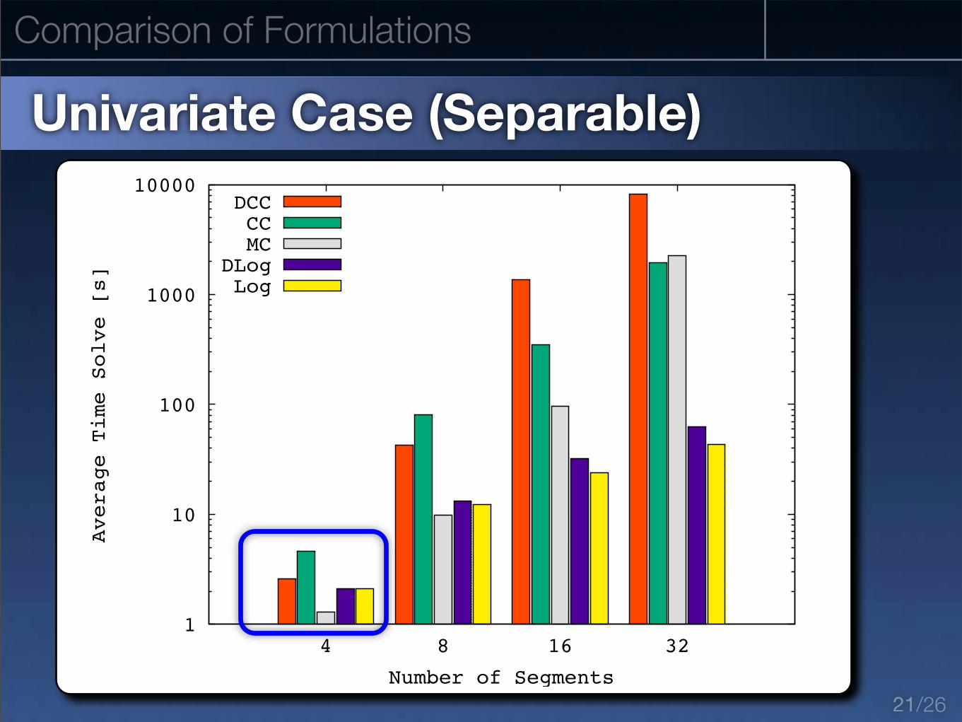
Instances

Transportation problems (10x10 & 5x2).

Univariate: Concave Separable Objective.

Multivariate: 2-commodity.

Functions: affine in k segments or k x k

grid triangulation (100 instances per k).

Solver: CPLEX 11 on 2.4Ghz machine.

Logarithmic versions of CC = Log,

DCC=DLog. /26


Computational Results

20

0 1 20

1

2

/26


Univariate Case (Separable)

21

1

10

100

1000

10000

4 8 16 32

Average Time Solve [s]

Number of Segments

DCCCCMC

DLogLog

/26


Multivariate Case (Non-Separable)

22

1

10

100

1000

10000

4x4 8x8 16x16


Grid Size

DCCCCMC

DLogLog

≤

0 2 4 50

1

4

3

2

/26

Lower Semicontinuous Functions

Lower Semicontinuous PLFs

23

f(x) :=

{

mP x + cP x ∈ P ∀P ∈ P

.P = {x ∈n

: aix ≤ bi ∀i ∈ {1, . . . , p},

aix < bi ∀i ∈ {p, . . . ,m}}

Finite family of

copolytopes

/26



23

f(x) :=

{


.P = {x ∈n

: aix ≤ bi ∀i ∈ {1, . . . , p},

aix < bi ∀i ∈ {p, . . . ,m}}

Finite family of

copolytopes

} { ∈ } {

f(x, y) :=

3 (x, y) ∈ (0, 1]2

2 (x, y) ∈ {(x, y) ∈ 2 : x = 0, y > 0}

2 (x, y) ∈ {(x, y) ∈ 2 : y = 0, x > 0}

0 (x, y) ∈ {(0, 0)}.

Figure 8(b) is slightly more complicated and its domain is ˜ = con

x

y

0

2

3

/26



23

f(x) :=

{


.P = {x ∈ n

: aix ≤ bi ∀i ∈ {1, . . . , p},

aix < bi ∀i ∈ {p, . . . ,m}}

Finite family of

copolytopes

} { ∈ } {

f(x, y) :=

3 (x, y) ∈ (0, 1]2

2 (x, y) ∈ {(x, y) ∈ 2 : x = 0, y > 0}

2 (x, y) ∈ {(x, y) ∈ 2 : y = 0, x > 0}

0 (x, y) ∈ {(0, 0)}.

Figure 8(b) is slightly more complicated and its domain is ˜ = con

x

y

0

2

3

/26


Lower Semicontinuous Models

Direct from Disjunctive Programming (Jeroslow and

Lowe)

“Extreme point” = DCC.

Traditional = Multiple Choice (MC).

Other models can be adapted to special types of

discontinuities (e.g. simple fixed charges).

MC, DCC, DLog are locally ideal and sharp.

Computations: 2-commodity FC discount function.

24

x

y

/26


Multivariate Lower Semicontinuous

25

1

10

100

1000

10000

4x4 8x8 16x16 32x32


Grid Size

DCCMC

DLog

/26

Final Remarks

Final Remarks

Unifying theoretical framework: allows for

multivariate non-separable and lower

semicontinuous functions.

First logarithmic formulations: Theoretically

strong and provides significant

computational advantage for large .

Revive forgotten formulations and

functions: MC and fixed charge

discount function.26

x

y

mixed integer programming models for non-separable ...jvielma/presentations/pwl_pitt_08.pdf ·...

Documents