American Journal of Industrial and Business Management, 2015, 5, 73-89 Published Online March 2015 in SciRes. http://www.scirp.org/journal/ajibm http://dx.doi.org/10.4236/ajibm.2015.53009

How to cite this paper: Sarkar, B., Sett, B.K., Goswami, A. and Sarkar, S. (2015) Mitigation of High-Tech Products with Probabilistic Deterioration and Inflations. American Journal of Industrial and Business Management, 5, 73-89. http://dx.doi.org/10.4236/ajibm.2015.53009

Mitigation of High-Tech Products with Probabilistic Deterioration and Inflations Biswajit Sarkar1*, Bimal Kumar Sett2, Adrijit Goswami3, Sumon Sarkar4 1Department of Industrial & Management Engineering, Hanyang University, Seoul, South Korea 2Department of Mathematics, Hooghly Mohsin College, Hooghly, India 3Department of Mathematics, Indian Institute of Technology, Kharagpur, India 4Department of Applied Mathematics with Oceanology and Computer Programming, Vidyasagar University, Midnapore, India Email: *bsbiswajitsarkar@gmail.com Received 3 January 2015; accepted 2 March 2015; published 5 March 2015

Copyright © 2015 by authors and Scientific Research Publishing Inc. This work is licensed under the Creative Commons Attribution International License (CC BY). http://creativecommons.org/licenses/by/4.0/

Abstract This paper describes a deteriorating inventory model with ramp-type demand pattern under stock-dependent consumption rate. The deterioration of the product is considered as probabilistic to make the research a more realistic one. The proposed model assumes partially backorder rate which follows a negative exponential with the waiting time. The effect of inflation and time value of money are incorporated into the model. The purpose of this study is to develop an optimal rep-lenishment policy so that the total profit is maximized. We provide a simple solution procedure to obtain the optimal solutions. Numerical examples along with graphical representations are pro-vided to illustrate the model. Sensitivity analysis of the optimal solution with respect to key para-meters of the model has been carried out and the implications are discussed.

Keywords Ramp-Type Demand, Stock-Dependent Consumption Rate, Partial Backorder, Inflation, Probabilistic Deterioration

1. Introduction In reality, deterioration of items during storage period is a realistic phenomenon in many inventory sectors. Controlling and regulating the deteriorating items are very difficult in practice. In storage system, fruits, vegeta-bles, foodstuffs, etc. deteriorate during their normal storage period. The deteriorating items cannot be used for its

*Corresponding author.

B. Sarkar et al.

74

original purpose. The loss of inventory due to deterioration cannot be ignored. Thus, it is very essential to control the deterioration of items. A model with exponentially decaying inventory was initially proposed by Covert and Philip [1]. Dye et al. [2] considered a deteriorating inventory model with time-varying demand and short-age-dependent partial backlogging. Chung and Wee [3] discussed a deteriorating inventory model for pricing policy with imperfect production, inspection planning, warranty period, and stock-level-dependant demand. Sana [4] established an inventory model for both ameliorating and deteriorating items with capacity constraint for storage. Wee et al. [5] proposed an optimal replenishment policy for deteriorating green products. Sett et al. [6] developed a two-warehouse inventory model with increasing demand and time-varying deterioration. They con-sidered the maximum lifetime of products. Always all deterioration functions are not deterministic type; it may follow probabilistic nature sometimes. Most recently, Sarkar [7] developed a production-inventory model for three different types of continuously distributed deterioration functions. Sarkar and Sarkar [8] explained a control- inventory problem with probabilistic deterioration. They solved the model with the help of Euler-Lagrange me-thod. Sarkar and Sarkar [9] developed an inventory model with time-varying demand and deterioration. Sarkar et al. [10] considered a deteriorating inventory model with variable demand. C��𝑎rdenas-Barr��𝑜n et al. [11] developed an improved solution procedure to solve a production model with reworking and multiple shipments. Sarkar and Saren [12] established a partial trade-credit model for retailer with exponentially deterioration. Sarkar et al. [13] considered a deteriorating inventory model with trade-credit policy for fixed lifetime products.

In classical inventory models, it is often assumed that shortages are either completely backlogged or completely lost. But in the real life, when shortages occur, it is observed that some customers may prefer their demands to be backordered, and some may refuse the backorder case. In this direction, Deb and Chaudhuri [14] were the first to incorporate shortages into inventory model—that model was an extension of Donaldson’s [15] model with shortages. Chang and Dye [16] developed an inventory model in which the backlogging rate is the reciprocal of a linear function of the waiting time. Cardenas-Barron [17] explained without using differential calculus how in-ventory model with shortages can be solved with using basic algebraic procedure. Teng et al. [18] extended the model in which the backlogging rate is any decreasing function of the waiting time up to the next replenishment. Sometimes managers prefer to use planned backorders to reduce the total system cost. In this direction, Carde-nas-Barron [19] presented an inventory model with reworking process at a single-stage manufacturing system with planned backorders. Sarkar et al. [20] described a production policy in order to find out an optimal safety stock, production lotsize, and reliability parameters. Sarkar et al. [21] developed an integrated inventory model with variable lead time, defective units, and delay in payments. Sarkar and Majumder [22] developed an integrated vendor-buyer supply chain model with vendors setup cost reduction. Sarkar and Sarkar [23] presented an im-proved inventory model with partial backlogging, time-varying deterioration, and stock-dependent demand. Most recently, Sarkar et al. [24] extended the inventory model with random defective rate, rework process, and variable backorders. Sarkar et al. [25] developed a continuous review inventory model with backorder price discount under controllable lead time.

Classical inventory model considers constant demand rate. However it is observed that the demand rate for electronic goods (e.g., hard disk, RAM, processor, mobile, etc.), new brand of consumer goods, seasonal products (fruits, e.g., mango, orange, etc.) increases linearly at the beginning up to a certain moment as time increases and then stabilizes to a constant rate until the end of the inventory cycle. To represent such type of demand pattern, the “term/ramp-type” is used. Mandal and Pal [26] were the first authors to introduce ramp-type demand in inventory model. Wu [27] developed an EOQ model with ramp-type demand, Weibull distributed deterioration and partial backlogging. Giri et al. [28] extended the model of Wu [27] with more generalized Weibull deterioration distri-bution. A model with partial backlogging was considered by Skouri et al. [29]. Sana [30] formulated an EOQ model over an infinite time horizon for deteriorating items with price-sensitive demand and partial backordering. Cardenas-Barron et al. [31] developed two easy and improved algorithms to determine jointly both the optimal replenishment lot size and the optimal number of shipments. Sarkar et al. [32] proposed a continuous review manufacturing inventory model with setup cost reduction, quality improvement, and a service level constraint.

The effects of inflation and time-value of money cannot be ignored for the present study. Several researchers have examined the inflationary effect on the inventory policy. Buzacott [33] was the first researcher to assume inflation in inventory model. Datta and Pal [34] presented the effect of inflation and time value of money on an inventory model with linear time-dependent demand rate and shortages. Jaggi et al. [35] considered a deteriorating inventory model under inflationary conditions using a discounted cash flow (DCF) approach over a finite planning horizon. Sarkar and Moon [36] extended an economic production quantity (EPQ) model with inflation in an im-

B. Sarkar et al.

75

perfect production system. Sarkar et al. [37] [38] developed two inventory models for imperfect production with inflation and time value of money.

This model is developed for deteriorating items with ramp-type demand under stock-dependent demand. In addition, different types of probabilistic deteriorations are considered in this model. Shortages are allowed which are backlogged. The effect of inflation and time value of money are incorporated into the model. The main pur-pose of this paper is to develop an optimal replenishment policy which maximizes the total profit per unit time. The necessary and sufficient conditions of the existence and the uniqueness of the optimal solutions are also provided. Sensitivity analysis of the optimal solution with respect to major parameters and their discursion is carried.

2. Notation and Assumptions To derive the model, following notation and assumptions are made:

2.1. Notation Q order quantity per cycle (units) θ probabilistic deterioration rate ( )tδ backlogging rate

r discount rate representing the time-value of money i inflation rate per unit time

r iρ = − discount rate minus inflation rate s selling price per unit ($/unit) Ca ordering cost per order ($/order) Ch unit inventory holding cost per week ($/unit/week) Cp purchasing cost per unit purchase ($/unit) Cb backorder cost per unit backorder ($/unit) Cl lost sell cost per unit ($/unit) µ the parameter of the ramp-type demand function (break point) (week) I(t) on-hand inventory level at time t t1 length of time in which the inventory level falls to zero (week) T fixed length of each ordering cycle (week)

( )1 1Z t total profit for Model I ($/week)

( )2 1Z t total profit for Model 2 ($/week)

2.2. Assumptions 1) The model is considered for a single item. 2) Deterioration rate θ is probabilistic and there is no replacement or repair of deteriorated units during the

period under consideration. 3) The demand rate D(t) is assumed to be a ramp-type function of time, i.e.,

( ) ( ) ( )0 0, 0D t D t t H t Dµ µ= − − − >

where ( )H t µ− is the Heaviside’s function as follows:

( )1 if0 if .

tH t

tµ

µµ

≥− = <

4) S(t) is the selling rate at time t, and it is influenced by the demand rate and the on-hand inventory according to relation

( )( ) ( ) ( )( ) ( )

, 0

, 0.

D t I t I tS t

D t I t

α+ >= ≤

where α is positive constant and I(t) is the on-hand inventory level at time t.

B. Sarkar et al.

76

5) Shortages are allowed and partially backlogged at a rate ( )tδ ; which is a decreasing function of time with ( ) ( ) ( )0 1, 0 1, and lim 0.tt tδ δ δ→∞≤ ≤ = = The cases with ( ) 1 or 0tδ = for all t correspond to complete back-

logging (or complete lost sales) models. 6) The effects of inflation and time-value of money are considered. 7) Lead time is assumed as negligible.

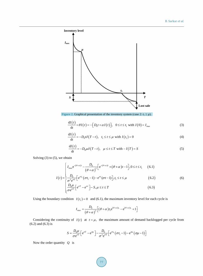
3. Model Formulation The model considers an inventory model for deteriorating items with ramp-type demand and stock-dependent selling rate. The replenishment at the beginning of the cycle brings the inventory level up to maxI . The inventory level decreases during the time interval [ ]10, t due to demand and deterioration of items, and falls to zero at 1t t= . Thereafter shortages occur during the period ( )1,t T , which are partially backlogged. The inventory level, ( ) ,0I t t T≤ ≤ satisfies the following differential equations

( ) ( ) ( ) ( )1 max

d, 0 , 0

dI t

I t S t t t I It

θ+ = − ≤ ≤ = (1)

( ) ( ) ( ) ( )1 1

d, , 0

dI t

S t T t t t T I tt

δ= − − ≤ ≤ = (2)

The solutions of these differential equations depend on the selling rate. There are two cases considering in this paper: (a) 1t µ≤ and (b) 1 .t µ≥ The fluctuation of the inventory level for the two cases is depicted in Figure 1 and Figure 2, respectively.

3.1. Model 1: t1 µ≤ In this case, the selling rate S(t) is

( )( )0 1

0 1

0

, 0,, .

D t I t t tS t D t t t

D t T

αµ

µ µ

+ ≤ ≤

= ≤ ≤ ≤ ≤

(1) and (2) are in the form

T

Inventory level

µ

Imax

S

t1

Lost sale

Figure 1. Graphical presentation of the inventory system (case 1: t1 ≤ µ).

B. Sarkar et al.

77

S

µ

t1

T

Lost sale

Inventory level

Imax

Figure 2. Graphical presentation of the inventory system (case 2: t1 ≥ µ).

( ) ( ) ( ) ( )0 1 max

d, 0 with 0

dI t

I t D t I t t t I It

θ α+ = − + ≤ ≤ = (3)

( ) ( ) ( )0 1 1

d, with 0

dI t

D t T t t t I tt

δ µ= − − ≤ ≤ = (4)

( ) ( ) ( )0

d, with

dI t

D T t t T I T St

µδ µ= − − ≤ ≤ − = (5)

Solving (3) to (5), we obtain

( )

( )

( )( ) ( ) ( )

( ) ( )

( )

1

0max 12

01 12

0

e e 1 ,0 6.1

e 1 e ( 1) , 6.2e

e e , 6.3e

t t

t tT

T tT

DI t t t

DI t t t t t

DS t T

θ α θ α

σ σσ

σ σσ

θ αθ α

σ σ µσ

µµ

σ

− + − + − + + − ≤ ≤ + = − − − ≤ ≤

− − ≤ ≤

(6)

Using the boundary condition ( )1 0I t = and (6.1), the maximum inventory level for each cycle is

( )( ) ( ) ( )1 10

max 12 e e 1t tDI t θ α θ αθ α

θ α+ + = + − + +

Considering the continuity of ( )I t at ,t µ= the maximum amount of demand backlogged per cycle from (6.2) and (6.3) is

( ) ( )10 012e e e 1 e 1

e etT

T T

D DS tσσ σµ σµ

σ σ

µσ σµ

σ σ = − − − − −

Now the order quantity Q is

B. Sarkar et al.

78

( )( ) ( ) ( )

( ) ( )

1 1

1

0 0max 12

012

e e 1 e ee

e 1 e 1e

t t TT

tT

D DQ I S t

Dt

θ α θ α σ σµσ

σ σµσ

µθ α

σθ α

σ σµσ

+ + = + = + − + + − +

− − − −

The total cost per cycle consists of the following four values (a) Ordering cost per cycle

( )0e d 1 e

T t Too

COC C tρ ρ

ρ− −= = −∫

(b) Purchase cost per cycle

( )0e d 1 e

T pt Tp

C QPC C Q tρ ρ

ρ− −= = −∫

(c) Holding cost per cycle

( )

( )( )

( )( )( ) ( ) ( ) ( )

1

1 1

1

1

0

1102 2

e d

1 e 1 1 e1e 1

e

t th

t tth

t

HC C I t t

ttC D

ρ

ρ ρθ α ρ

ρ

ρ θ α ρθ αρθ α ρθ α

−

− −+ +

=

− − + − ++ − = − ++ + +

∫

(d) Backlogging cost per cycle

( )( ) ( )( )

( ) ( )

( ) ( )

( )[ ] ( ) ( ) ( )

( )

1

1 1

1 1

102

12

e d e d

1 e e e e e e

e

e e 1 e e e

Tt tb t

t tT T

bT

t t T

BC C I t t I t t

tC D

t

µ ρ ρµ

σ ρ σρ ρ ρµ σµ

σ

σ ρ σ ρ µ σ ρ σ ρ σ ρ µ

σ

ρσ

σ σ µσρ σσ ρ

− −

− − − −

− − − − −

= − + − − − + − =

− − − + + +−−

∫ ∫

(e) Lost sale cost per cycle

( ) ( )

( ) ( ) ( ) ( ) ( )

( )[ ]

1

1 1 1

0 0

1 10 2 2

1 e d 1 e d

e e e e e 1 e e

e

Tt tl t

T t t t T

l T

LC C D t T t t D T t t

t tC D

µ ρ ρµ

σ ρ σ ρ σ ρ µ σ ρ ρ ρ ρµ

σ

δ µ δ

ρ σ µ ρ ρµρσ ρ

− −

− − − − − − −

= − − + − − − − + − + − − = + −

∫ ∫

(f) Sale revenue per cycle

( ) ( ) ( )( ) ( ) ( ) ( ) ( )

( )[ ]

( )( )

( )( ) ( ) ( )

1

1

1 1 1

1 1

1

1

0

1 10 2 2

112 2

e d e d

e e e e 1 e 1

e

1 e [1 1 e ]1e 1

e

t Tt tt

t T t t

T

t tt

t

SR s S t t S t T t t

t tsD

tt

ρ ρ

σ ρ σ ρ µ σ ρ σ ρ ρ

σ

ρ ρθ α ρ

ρ

δ

σ ρ µ ρρσ ρ

ρ θ α ρθ ααρθ α ρθ α

− −

− − − − −

− −+ +

= + − − + − − − + = + −

− − + − ++ − + − + + ++

∫ ∫

Therefore, the total profit per unit time under the effect of inflation and time-value of money is

B. Sarkar et al.

79

( ) ( )

( )( ) ( )

( )( ) ( )

( ) ( ) ( ) ( ) ( ) ( )

( )

( )

1 1 1

1

1 11

1 1

1 102 2

11

2 2

1

1 e 1 1 1 e 1 ee

e e e e1 1 e

e

t t th

t

t T tt

T

l

Z t SR OC PC HC BC LCT

t tD s CT

tts

C

θ α ρ ρ ρ

ρ

σ ρ σ ρ µ σ ρ σ ρρ

σ

θ α θ α ραρρθ α ρθ α

σ ρ µρ

ρ σ ρ

ρ σ

+ + − −

− − − −−

= − + + + +

+ − − + − +− − = − + + ++ − + − − − + + +

−

−−

( ) ( ) ( ) ( )

( )[ ]

( ) ( )

( )( ) ( )

( ) ( )

( )[ ] ( ) [ ] ( )

1 1 1

1 1

1 1

1 12 2

1

2

12

e e e e e 1 e e

e

e e 1 e e e e e e

e

e e 1 e 1 e

T t t t T

T

T t tT T

bT

t t

t t

tC

t

σ ρ σ ρ σ ρ µ σ ρ ρ ρ ρµ

σ

σ ρ µ σ ρ σ ρ σρ ρ ρµ σµ

σ

σ ρ σ ρ µ σ ρ σ ρ µ

µ ρ ρµρσ ρ

σ σµρ σ µρσ

σ σ µσ

µ σ ρ

− − − − − − −

− − − − − −

− − − −

− + − + − − + −

− − − + − − +−

− − − − + +− ( ) ( )

0

1 e T

o pC C QD

ρ

ρ σ µ ρ

− − − + −

(7)

Our objective is to obtain the optimal value of 1t such that the average profit ( )1 1Z t is maximum.

3.2. Model 2: t1 µ≥ In this case, the selling rate S(t) is

( )( )( )

0

0 1

0 1

, 0

,, .

D t I t t

S t D I t t tD t t T

α µ

µ α µµ

+ ≤ ≤

= + ≤ ≤ ≤ ≤

Hence, (1) and (2) reduce to the following equations

( ) ( ) ( ) ( )0 max

d, 0 with 0

dI t

I t D t I t t I It

θ α µ+ = − + ≤ ≤ = (8)

( ) ( ) ( ) ( )0 1 1

d, with 0

dI t

I t D I t t t I tt

θ µ α µ+ = − + ≤ ≤ = (9)

( ) ( ) ( )0 1 1

d, with 0

dI t

D T t t t T I tt

µδ= − − ≤ ≤ = (10)

Solving Equations (8) to (10) with the boundary conditions, we obtain

( )

( )

( )( ) ( ) ( )

( )( )( ) ( )

( )

1

1

0max 2

01

01

e e 1 , 0 11.1

e 1 , 11.2

e e , 11.3e

t t

t t

t tT

DI t t

DI t t t

Dt t T

θ α θ α

θ α

σ σσ

θ α µθ α

µµ

θ αµ

σ

− + − +

+ −

− + + − ≤ ≤ + = − ≤ ≤ +

− ≤ ≤

(11)

Considering the continuity of ( )I t at t µ= the maximum inventory level maxI from Equations (11.1) and (11.2) is

B. Sarkar et al.

80

( )( )

( )( )10 0

max 2e e 1tD DI θ α θ α µµ

θ α θ α+ + = − − + +

Putting t T= in (11.3), the maximum amount of demand backlogged per cycle can be obtained as

( ) 10 e ee

tTT

DS I T σσ

σ

µσ

≡ − = −

Now the order quantity Q is

( )( )

( )( )1 10 0 0

max 2e e 1 e ee

t tTT

D D DQ I S θ α θ α µ σσ

σ

µ µθ α σθ α

+ + = + = − − + − + + (12)

The total cost per cycle consists of the following four values (a) Ordering cost per cycle

( )0e d 1 e

T t Too

COC C tρ ρ

ρ− −= = −∫

(b) Purchase cost per cycle

( )0e d 1 e

T pt Tp

C QPC C Q tρ ρ

ρ− −= = −∫

(c) Holding cost per cycle

( ) ( )

( )( ) ( ) ( ) ( ) ( )

( )

1

1 11

0

02 2

e d e d

e e e ee 1 e

tt th

t tth

HC C I t t I t t

C D

µ ρ ρµ

θ α θ α µρ ρµρ ρµ µ θ αρµ θ α θ α ρ

θ α ρρθ α

− −

+ +− −− −

= + + − − + + − − + − = + + ++

∫ ∫

(d) Backlogging cost per cycle

( )( ) ( )

( )

11 1

1

0e ee e e

e de

T tt tTT t b

b Tt

C DBC C I t t

σ ρ σ ρσ ρρρ

σ

µρ σ ρσ

− −−−−

− − = − = + −

∫

(e) Lost sale cost per cycle

( )( ) ( )

( )11

10 0

e e e e ]1 e de

T tt TT tl l Tt

LC C D T t t C Dσ ρ σ ρρ ρ

ρσµ δ µ

ρ σ ρ

− −− −− − − = − − = − −

∫

(f) Sale revenue per cycle

( ) ( ) ( )( ) ( )

( )

( )( ) ( ) ( ) ( ) ( )

( )

1

1

11

1 11

0

0 2

2 2

e d e d

e e e1 e e

e e e ee 1 e

t Tt tt

T tTt

t tt

SR s S t t S t T t t

sD

ρ ρ

σ ρ σ ρσρρµ

θ α θ α µρ ρµρ ρµ

δ

µρµσ ρρ

µ θ αρµ θ α θ α ραθ α ρρθ α

− −

− −−−−

+ +− −− −

= + −

−− − = +−

+ − − + + − − + − + + + ++

∫ ∫

Total profit per unit time under the effect of inflation and time-value of money is

B. Sarkar et al.

81

( ) ( )

( )( ) ( ) ( ) ( ) ( )

( )( ) ( )

( )( ) ( )

( )

1 11

111

2 1

02 2

2

1

e e e ee 1 e

e e e1 e e e e ee

t tth

T tT T tt t

l T

Z t SR OC PC HC BC LCT

D s CT

s C

θ α θ α µρ ρµρ ρµ

σ ρ σ ρσ σ ρ σ ρρ ρρµ

σ

µ θ αρµ θ α θ α ραθ α ρρθ α

µρµ µσ ρρ σ ρ

+ +− −− −

− −− − −− −−

= − + + + +

+ − − + + − − + −− = + + + +

−− − − + + + − − −

( ) ( )

( ) ( )

1

11 1

0

e

e ee e e 1 e

e

T

T tt tT Tb

o pT

CC C Q

D

ρ

σ ρ σ ρσ ρρ ρ

σ

ρ

µρ σ ρ ρσ

−

− −−− −

−

− − − − + − + −

(13)

Our objective is to find the optimal value of 1t such that the average profit ( )2 1Z t is maximum. The total profit function of the system over [ ]0,T takes the form

( )( )( )

1 1 11

2 1 1

if

if

Z t tZ t

Z t t

µ

µ

≤= ≥

(14)

It is easy to check that this function is continuous at µ .

3.3. Solution Procedure In this section, we derive results which ensure the necessary and sufficient conditions of the existence and uni-queness of the optimal solution to maximize the total profit.

From (7), for 1t µ≤ ( ) ( )1 1 1 0

11

dd

Z t t DF t

t T= (15)

where

( ) ( ) ( ) ( )

( )( )

( ) ( ) ( ) ( )

11 1 1

11 1

1

1 e e e e ee

1 ee 1 e ee

t Tt t t Tbl T

Ttp t T th

t

CF t s C

Cs C

σ ρ σρ σ ρ ρσ

ρθ α ρσ θ α

ρ

ρ

αθ α ρ ρ

− −− − −

−+ +− +

= + − + −

− − − + + − + +

(16)

On the other hand we have

( ) ( ) ( )0 1 e 1 e 1 ee

p T T Tbl T

C CF s C ρ σ ρ

σρ ρ− − −

= + − − − + −

(17)

and

( ) ( )( )

( ) ( ) ( )( )e e 1 e 1 epT Th T TCs CF T θ α θ αρ ρα

θ α ρ ρ+ +− −− = − + − − + +

(18)

Taking first order derivative of ( )1F t with respect to 1t , we obtain

( ) ( ) ( ) ( )

( ) ( ) ( ) ( )

( ) ( )( )

11

11

1

ee 1 e

e

ee e 1e

tp th Tb

l T

tt Th

l p bT

Cs CCt s C

s Cs C C C

σ ρθ αρ

σ

σρ ρ

σ ρ

ασ ρθ α

ρ θ α ρ ρ

α σρθ α ρ ρ

−+−

−+

−− = − − + + − + + +

− + − − + − − + +

(19)

B. Sarkar et al.

82

Now if ( )1 0t < and ( ) ( )0 0, 0,F F T> < then ( )1F t is strictly decreasing function of 1t . Therefore the equation

( )1 0F t = (20)

Has a unique root ( )*1 0,t T∈ for which

( ) ( )*

1 1

2 *1 1 *0 1

121

d0

dt t

Z t D tt

Tt=

= < (21)

From (13), for 1tµ ≤

( ) ( )1 1 01

1

dd

Z t DF t

t Tµ

= (22)

( ) ( )2

1 1 012

1

ddZ t D

tTtµ

= (23)

where ( )1F t is given by (16). The above analysis shows that two functions ( )1 1Z t and ( )2 2Z t have the unique and same unstrained

maximum point ( )*1 0,t T∈ , which is determined by (16).

Now if ( )1 0t < and ( ) ( )0 0, 0,F F T> < then ( )1F t is strictly decreasing function of 1t . Hence

( )1 0F t = has a unique root ( )*1 0,t T∈ .

4. Numerical Experiments To derive the optimal solution, we solve two examples that consist of the different situation of the ramp-type demand and the deterioration rates. Let us consider the following parametric values: 0 400D = , $50 orderoC = ,

$20 units = , $3 unit unit timehC = , $15 unitpC = , $5 unitbC = , $8 unitlC = , 0.1α = , 0.04ρ = , 0.02σ = , 0.05θ = , 1 weekT = .

4.1. Example 1 We assume that 0.7µ = then solving the equation ( )1 0F t = the optimal replenishment cycle time *

1 0.6010t = satisfying *

1t µ≤ and the maximum total profit per unit of time ( )*1 1 $617.784 weekZ t = . The graphical re-

presentation of the pro t function versus the replenishment time is presented in Figure 3. Now examine whether the optimal solution is unique.

( ) ( ) ( )1 8.54 0, 0 5.07 0, and 3.44 0.t F F T= − < = > = − <

Hence *1t is a unique solution.

4.2. Example 2 We assume that 0.4µ = , then solving the equation ( )1 0F t = the optimal replenishment cycle time *

1 0.6010t = satisfying *

1t µ≥ and the maximum total profit per unit of time ( )*2 1 $423.40 weekZ t = . The graphical repre-

sentation of the profit function versus the replenishment time is presented in Figure 4. Now examine whether the optimal solution is unique.

( ) ( ) ( )1 8.54 0, 0 5.07 0, and 3.44 0.t F F T= − < = > = − <

Hence *1t is a unique solution.

From above numerical examples we can conclude that the optimal total profit is maximum when μ = 0.7 i.e., for Model I. Now we consider different continuous probabilistic deterioration functions. Based on that, we have done our numerical experiments with the same parametric values as in Example 1.

B. Sarkar et al.

83

Profit

Time

Figure 3. Graphical presentation of total profit function versus time (Example 1).

Profit

Time

Figure 4. Graphical presentation of total profit function versus time (Example 2).

4.3. Example 3 Here we consider ( )( ) ( ) 2E f x a bθ = = + (Sarkar and Sarkar [8]) where ( )f x follows a uniform distribution, and a b< . We consider the parametric values 0.05 and 0.15a b= = and the rest of the values are the same as in Example 1. Then, the optimal solution is *

1 0.5490t = week and * $597.393 weekZ = .

4.4. Example 4 Here we consider ( )( ) ( ) 3E f x a b cθ = = + + where ( )f x follows a triangular distribution, and a c b≤ ≤ . We consider the parametric values 0.05, 0.15 and 0.13a b c= = = and the rest of the values are the same as in Example 1. Then, the optimal solution is *

1 0.5394t = week and * $593.91 weekZ = .

4.5. Example 5 Here we consider ( )( ) ( )4 6E f x a m bθ = = + + where ( )f x follows a double triangular distribution, and a m b≤ ≤ . We consider the parametric values 0.05, 0.13 and 0.15a m b= = = and the rest of the values are the same as in Example 1. Then, the optimal solution is *

1 0.5302t = week and * $590.597 weekZ = .

B. Sarkar et al.

84

4.6. Example 6 Here we consider ( )( ) ( )E f xθ α α β= = + where ( )f x follows a beta distribution, and 𝛼𝛼 ≥ 0 and 0β ≥ . We consider the parametric values 0.05 and 0.15α β= = and the rest of the values are the same as in Example 1. Then, the optimal solution is *

1 0.4329t = week and * $559.053 weekZ = . The graphical representation of Examples 3, 4, 5, and 6 are depicted in Figure 5.

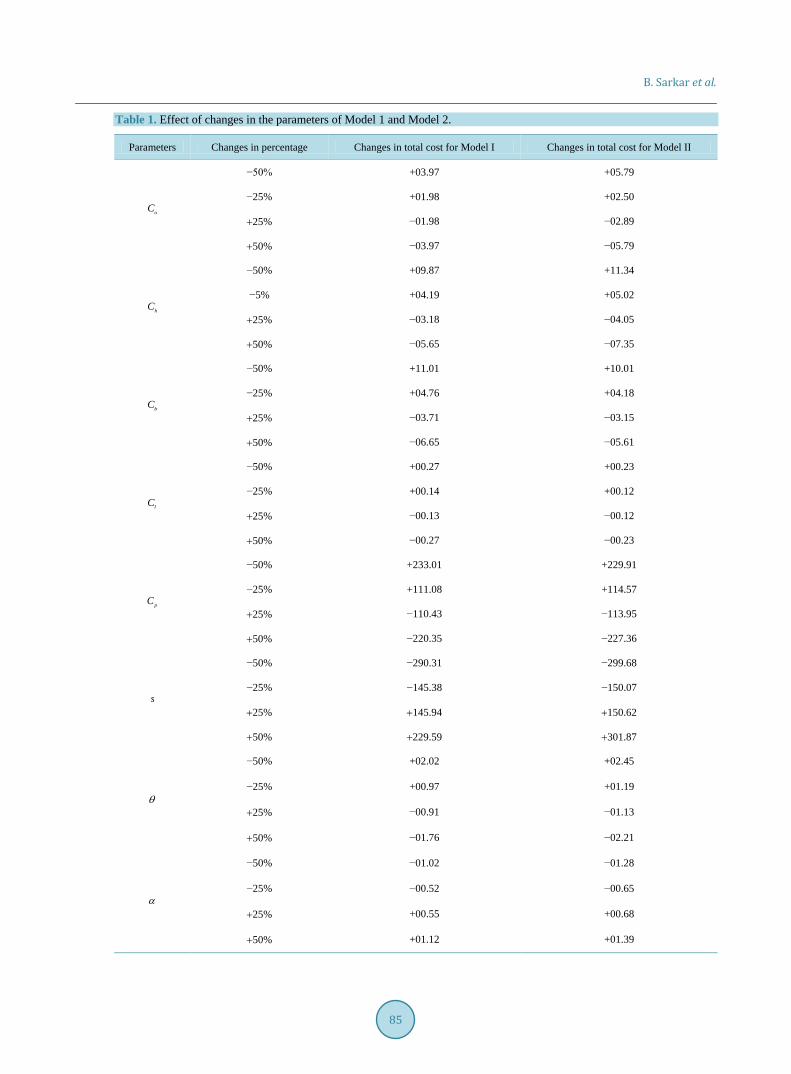
5. Sensitivity Analysis We now study the effects of changes in parameters such as , , , , , , , ando h b l pC C C C C s θ α on optimal total profit. The sensitivity analysis is performed by changing each of the parameters by 50%, 25%, 25%, and 50%− − + taking one parameter at a time while keeping the remaining parameters unchanged. The results of Example 1 and Ex-ample 2 are presented in Table 1.

From Table 1, the discussion of sensitivity analysis of the key parameters is as follows: From the above table we can conclude that ( )1 1Z t and ( )2 1Z t are highly sensitive towards change in pC

and s whereas slightly sensitive in , ,lC θ and α . On the other hand, ( )1 1Z t and ( )2 1Z t are moderately sensitive towards change in , ,o hC C and .bC

6. Special Cases In this section, we will discuss some special cases that influence the total profit.

6.1. Case 1 0σ = implies a complete backlogging inventory model. In this case the total profit function is as follows

( ) ( )( )

( )( ) ( )( ) ( ) ( )( )

( )( )

( ) ( )

( )( )

11 11

1

1 1011 1 2 2

2 2 21

130

212 2

e e 1 1 1 e 11 e

ee 1 e 1 e 1 e

2

1 e1 e e 2 22

tt tth

Tt T Tb o

TTp

t ts CDZ tT

tC Ct TD

Cs t

α θ ρρ ρρ

ρρ ρ µρ ρ

ρµρ ρ

α θ α θ ραρ α θ ρ ρθ α

ρ µρ ρµ ρ

ρρ

µρρρ α θ

+ +− −−

−− − − −

−− −

− + − + − +− − = + − + ++ + − + + − + − − −

− − −+ − − + −

+

( )

( )

( ) 1121

122 ee 2

tt t Ttα θα θ

µα θα θ

++ + + −

+ +

Uniform distribution Trianguler distribution

Double trianguler distribution Beta distribution

Profit

Time

Figure 5. Graphical presentation of total profit versus time under different probabilistic deterioration functions (Exam-ple 3 - 6).

B. Sarkar et al.

85

Table 1. Effect of changes in the parameters of Model 1 and Model 2.

Parameters Changes in percentage Changes in total cost for Model I Changes in total cost for Model II

oC

−50% +03.97 +05.79

−25% +01.98 +02.50

+25% −01.98 −02.89

+50% −03.97 −05.79

hC

−50% +09.87 +11.34

−5% +04.19 +05.02

+25% −03.18 −04.05

+50% −05.65 −07.35

bC

−50% +11.01 +10.01

−25% +04.76 +04.18

+25% −03.71 −03.15

+50% −06.65 −05.61

lC

−50% +00.27 +00.23

−25% +00.14 +00.12

+25% −00.13 −00.12

+50% −00.27 −00.23

pC

−50% +233.01 +229.91

−25% +111.08 +114.57

+25% −110.43 −113.95

+50% −220.35 −227.36

s

−50% −290.31 −299.68

−25% −145.38 −150.07

+25% +145.94 +150.62

+50% +229.59 +301.87

θ

−50% +02.02 +02.45

−25% +00.97 +01.19

+25% −00.91 −01.13

+50% −01.76 −02.21

α

−50% −01.02 −01.28

−25% −00.52 −00.65

+25% +00.55 +00.68

+50% +01.12 +01.39

B. Sarkar et al.

86

The necessary condition for ( )11 1Z t to be maximized is ( )11 1

1

d0

dZ t

t= which implies

( )( )

( )( ) ( ) ( )( ) ( )1

1 11

1 e 1 ee 1 e e

e

tTpth tT

bt

Cs CC

α θρα θ ρ ρρ

ρ

αρ

ρα θ ρ

+−

+ + −−− −−

− + = −+ +

6.2. Case 2 0ρ = , i.e., the inflationary effect is not considered. For this special case the total profit function is given by

( ) ( )( )

( ) ( ) ( )( )

( ) ( )

( )( )

( )( )

( )( )

( )

1

1

1

1

1

2210

12 1 13

12

21 1 12

2 21

1

2

2

1

1 e 12

e e 1 e 2

e

2 e ee e e 2 1

e

e e 1 e 12e

th

t T

T

ttTb

T

t TlT

s C tDZ t tT

t ts

C T t t T t

tC t T

α θ

σµσ σ

σ

σ µσσσ µσ

σ

σµσ σσ

α α θα θ

θ α

σ σ µ σ

σ

µ µ σ σσσ

µ σσ σ µ σ

σ

+ − + = − + + −

+ − + − + + +

− − + − + + − + + −

+− + − + − + − 0 0

po QCCD D

− −

The necessary condition for ( )12 1Z t to be maximized is ( )12 1

1

d0

dZ t

t= which implies

( ) ( )( ) ( ) ( )( )( ) ( ) ( ) ( )( )

1

1 1 1 11

e 11 e e e e

tht T t T t t T

l b p

s Cs C C t T C

θ α

σ σ θ α σα

θ α

+

− − + −− −

+ − + = − + −+

6.3. Case 3 0ρ = and 0σ = implies the inflationary effect is not considered and the backlogging is complete. For this

special case, the total profit function is given by

( ) ( )( ) ( ) ( )( )

( ) ( ) ( )1 1 21

3 21 1

1013 1 2

2 2

0

e e 12 1

2( )

6 3 2 2 2

t th

p p

ob

s C tD tZ t s C T CT

Ct t TT TCD

θ α θ αα θ αµµ µ

θ α θ α

µ µµ µ µ

+ + − + − += − − + − − + +

− + − − + −

The necessary condition for ( )13 1Z t to be maximized is ( )13 1

1

d0

dZ t

t= which implies

( ) ( )( )

( )( ) ( )11e 1

p h p ts

s C C CC t Tθ α

α θ

θ α+

− − + − = −+

6.4. Example 7 We use the same parametric values as in Example 2 and we obtain the results for special cases which is listed out in Table 2. The graphical representation of the profit function versus the replenishment time for special Case 1, Case 2, and Case 3 are presented in Figure 6.

B. Sarkar et al.

87

Table 2. Summary of the optimal solutions under different cases.

Special cases Time (week) Cost ($/week)

Case 1 ( )0σ = 0.5918 622.692

Case 2 ( )0ρ = 0.6054 649.811

Case 3 ( )0 and 0σ ρ= = 0.5953 654.853

Case 3 Case 2 Case 1

Profit

Time

Figure 6. Graphical presentation of total profit versus time for special cases (Example 7).

7. Conclusion In this marketing environment, when a new brand of consumer goods is launched, the demand of goods increas-es quickly to a certain moment and after some time it stabilizes. Finally, it becomes almost constant. Keeping this type of demand pattern in mind, we considered demand as a ramp-type function of time. To make the re-search a more realistic one, four different types of continuous probabilistic deterioration functions are consi-dered here. The associated profit function was maximized at the optimal values of decision variables. A unique solution procedure was provided as an optimal solution. Some numerical examples, graphical representations, special cases, and sensitivity analysis were given to illustrate the model. There are several extensions of this work that can constitute future research related in this field. This model can be extended in several ways, like multi-item inventory models, and reliability of the items. Another interesting idea is to consider fuzzy demand case.

Acknowledgements The authors would like to thank the reviewers for their helpful comments to improve the paper. The authors are grateful to Guest Editor Professor S. S. Sana for his useful comments. This work was supported by the research fund of Hanyang University (HY-2014-N, Project number 201400000002202) for new faculty members.

References [1] Covert, R.P. and Philip, G.C. (1973) An EOQ Model for Items with Weibull Distribution Deterioration. AIIE Transac-

tions, 5, 323-326. http://dx.doi.org/10.1080/05695557308974918 [2] Dye, C.Y., Chang, H.J. and Teng, J.T. (2006) A Deteriorating Inventory Model with Time-Varying Demand and

Shortage-Dependent Partial Backlogging. European Journal of Operational Research, 172, 417-429. http://dx.doi.org/10.1016/j.ejor.2004.10.025

[3] Chung, C.J. and Wee, H.M. (2008) An Integrated Production-Inventory Deteriorating Model for Pricing Policy Consi-

B. Sarkar et al.

88

dering Imperfect Production, Inspection Planning and Warranty-Period and Stock-Level-Dependant Demand. Interna-tional Journal of System Science, 39,823-837. http://dx.doi.org/10.1080/00207720801902598

[4] Sana, S.S. (2010) Demand Influenced by Enterprises Initiatives—A Multi-Item EOQ Model for Deteriorating and Ameliorating Items. Mathematical and Computer Modelling, 52, 284-302. http://dx.doi.org/10.1016/j.mcm.2010.02.045

[5] Wee, H.M., Lee, M.C., Yu, J.C.P. and Wang, C.E. (2011) Optimal Replenishment Policy for a Deteriorating Green Product: Lifecycle Costing Analysis. International Journal of Production Economics, 133, 603-611. http://dx.doi.org/10.1016/j.ijpe.2011.05.001

[6] Sett, B.K., Sarkar, B. and Goswami, A. (2012) A Two-Warehouse Inventory Model with Increasing Demand and Time Varying Deterioration. Scientia Iranica: E, 19, 1969-1977. http://dx.doi.org/10.1016/j.scient.2012.10.040

[7] Sarkar, B. (2013) A Production-Inventory Model with Probabilistic Deterioration in Two-Echelon Supply Chain Man-agement. Applied Mathematical Modelling, 37, 3138-3151. http://dx.doi.org/10.1016/j.apm.2012.07.026

[8] Sarkar, M. and Sarkar, B. (2013) An Economic Manufacturing Quantity Model with Probabilistic Deterioration in a Production System. Economic Modelling, 31, 245-252. http://dx.doi.org/10.1016/j.econmod.2012.11.019

[9] Sarkar, B. and Sarkar, S. (2013) Variable Deterioration and Demand—An Inventory Model. Economic Modelling, 31, 548-556. http://dx.doi.org/10.1016/j.econmod.2012.11.045

[10] Sarkar, B., Saren, S. and Wee, H.M. (2013) An Inventory Model with Variable Demand, Component Cost and Selling Price for Deteriorating Items. Economic Modelling, 30, 306-310. http://dx.doi.org/10.1016/j.econmod.2012.09.002

[11] Cárdenas-Barrón, L.E., Sarkar, B. and Treviño-Garza, G. (2013) An Improved Solution to the Replenishment Policy for the EMQ Model with Rework and Multiple Shipments. Applied Mathematical Modelling, 37, 5549-5554. http://dx.doi.org/10.1016/j.apm.2012.10.017

[12] Sarkar, B. and Saren, S. (2014) Partial Trade-Credit Policy of Retailer with Exponentially Deteriorating Items. Interna-tional Journal of Applied and Computational Mathematics. http://dx.doi.org/10.1007/s40819-014-0019-1

[13] Sarkar, B., Saren, S. and Cárdenas-Barrón, L.E. (2014) An Inventory Model with Trade-Credit Policy and Variable Deterioration for Fixed Lifetime Products. Annals of Operations Research. http://dx.doi.org/10.1007/s10479-014-1745-9

[14] Deb, M. and Chaudhuri, K.S. (1987) A Note on the Heuristic for Replenishment of Trended Inventories Considering Shortages. Journal of Operational Research Society, 38, 459-463.

[15] McDonald, J.J. (1979) Inventory Replenishment Policies-Computational Solutions. Journal of Operational Research Society, 30, 933-936. http://dx.doi.org/10.2307/3009548

[16] Chang, H.J. and Dye, C.Y. (1999) An EOQ Model for Deteriorating Items with Time Varying Demand and Partial Backlogging. Journal of Operational Research Society, 50, 1176-1182. http://dx.doi.org/10.2307/3010088

[17] Cárdenas-Barrón, L.E. (2011) The Economic Production Quantity (EPQ) with Shortage Derived Algebraically. Inter-national Journal of Production Economics, 70, 289-292. http://dx.doi.org/10.1016/S0925-5273(00)00068-2

[18] Teng, J.T., Chang, H.J., Dye, C.Y. and Hung, C.H. (2002) An Optimal Replenishment Policy for Deteriorating Items with Time-Varying Demand and Partial Back-Logging. Operations Research Letters, 30, 387-393. http://dx.doi.org/10.1016/S0167-6377(02)00150-5

[19] Cárdenas-Barrón, L.E. (2009) Economic Production Quantity with Rework Process at a Single-Stage Manufacturing System with Planned Backorders. Computer & Industrial Engineering, 57, 1105-1113. http://dx.doi.org/10.1016/j.cie.2009.04.020

[20] Sarkar, B., Sana, S. and Chaudhuri, K. (2010) Optimal Reliability, Production Lotsize and Safety Stock: An Economic Manufacturing Quantity Model. International Journal of Management Science and Engineering Management, 5, 192- 202.

[21] Sarkar, B., Gupta, H., Chaudhuri, K. and Goyal, S.K. (2014) An Integrated Inventory Model with Variable Lead Time, Defective Units and Delay in Payments. Applied Mathematics and Computation, 237, 650-658. http://dx.doi.org/10.1016/j.amc.2014.03.061

[22] Sarkar, B. and Majumder, A. (2013) Integrated Vendor Buyer Supply Chain Model with Vendor’s Setup Cost Reduc-tion. Applied Mathematics and Computation, 224, 362-371. http://dx.doi.org/10.1016/j.amc.2013.08.072

[23] Sarkar, B. and Sarkar, S. (2013) An Improved Inventory Model with Partial Backlogging, Time Varying Deterioration and Stock-Dependent Demand. Economic Modelling, 30, 924-932. http://dx.doi.org/10.1016/j.econmod.2012.09.049

[24] Sarkar, B., Cárdenas-Barrón, L.E., Sarkar, M. and Singgih, M.L. (2014) An Economic Production Quantity Model with Random Defective Rate, Rework Process and Backorders for a Single Stage Production System. Journal of Manufac-turing System, 33, 423-435. http://dx.doi.org/10.1016/j.jmsy.2014.02.001

[25] Sarkar, B., Mandal, B. and Sarkar, S. (2015) Quality Improvement and Backorder Price Discount under Controllable

B. Sarkar et al.

89

Lead Time in an Inventory Model. Journal of Manufacturing Systems, 35, 26-36. http://dx.doi.org/10.1016/j.jmsy.2014.11.012

[26] Mandal, B. and Pal, A.K. (1998) Order Level Inventory System with Ramp Type Demand Rate for Deteriorating Items. Journal of Interdisciplinary Mathematics, 1, 49-66. http://dx.doi.org/10.1080/09720502.1998.10700243

[27] Wu, K.S. (2001) An EOQ Inventory Model for Items with Weibull Distribution Deterioration, Ramp-Type Demand Rate and Partial Backlogging. Production Planning & Control, 12, 787-793. http://dx.doi.org/10.1080/09537280110051819

[28] Giri, B.C., Jalan, A.K. and Chaudhuri, K.S. (2003) Economic Order Quantity Model with Weibull Deterioration Dis-tribution, Shortage and Ramp-Type Demand. International Journal of System Science, 34, 237-243. http://dx.doi.org/10.1080/0020772131000158500

[29] Skouri, K., Konstantaras, I., Papachristos, S. and Ganas, I. (2009) Inventory Models with Ramp Type Demand Rate, Partial Backlogging and Weibull Deterioration Rate. European Journal of Operational Research, 192, 79-92. http://dx.doi.org/10.1016/j.ejor.2007.09.003

[30] Sana, S.S. (2010) Optimal Selling Price and Lotsize with Time Varying Deterioration and Partial Backlogging. Applied Mathematics and Computation, 217, 185-194. http://dx.doi.org/10.1016/j.amc.2010.05.040

[31] Cárdenas-Barrón, L.E., Sarkar, B. and Treviño-Garza, G. (2013) Easy and Improved Algorithms to Joint Determination of the Replenishment Lot Size and Number of Shipments for an EPQ Model with Rework. Mathematical and Compu-tational Applications, 18, 132-138.

[32] Sarkar, B., Chaudhuri, K. and Moon, I. (2015) Manufacturing Setup Cost Reduction and Quality Improvement for the Distribution Free Continuous-Review Inventory Model with a Service Level Constraint. Journal of Manufacturing Systems, 34, 74-82. http://dx.doi.org/10.1016/j.jmsy.2014.11.003

[33] Buzacott, J.A. (1975) Economic Order Quantities with Inflation. Operational Research Quarterly, 26, 553-558. http://dx.doi.org/10.1057/jors.1975.113

[34] Datta, T.K. and Pal, A.K. (1991) Effects of Inflation and Time-Value of Money on an Inventory Model with Linear Time-Dependent Demand Rate and Shortages. European Journal of Operational Research, 52, 326-333. http://dx.doi.org/10.1016/0377-2217(91)90167-T

[35] Jaggi, C.K., Aggarwal, K.K. and Goel, S.K. (2006) Optimal Order Policy for Deteriorating Items with Inflation In-duced Demand. International Journal of Production Economic, 103, 707-714. http://dx.doi.org/10.1016/j.ijpe.2006.01.004

[36] Sarkar, B. and Moon, I. (2011) An EPQ Model with Inflation in an Imperfect Production System. Applied Mathematics and Computation, 217, 6159-6167. http://dx.doi.org/10.1016/j.amc.2010.12.098

[37] Sarkar, B., Sana, S.S. and Chaudhuri, K.S. (2011) An Imperfect Production Process for Time Varying Demand with Inflation and Time Value of Money: An EMQ Model. Expert System with Application, 38, 13543-13548.

[38] Sarkar, B., Mandal, P. and Sarkar, S. (2014) An EMQ Model with Price and Time Dependent Demand under the Effect of Reliability and Inflation. Applied Mathematics and Computation, 231, 414-421. http://dx.doi.org/10.1016/j.amc.2014.01.004