mitigating supply risk: dual sourcing or process...
TRANSCRIPT

Mitigating Supply Risk: Dual Sourcing or ProcessImprovement?
Yimin WangW.P. Carey School of Business, Arizona State University
Wendell Gilland, Brian TomlinKenan-Flagler Business School, University of North Carolina
September 26, 2008. Last revised June 1, 2009.
Surveys suggest that supply chain risk is a growing issue for executives and that supplier reliability is of
particular concern. A common mitigation strategy observed in practice is for the buying firm to expend
effort improving the reliability of its supply base. We explore a model in which a firm can source from
multiple suppliers and/or exert effort to improve supplier reliability. For both random capacity and random
yield types of supply uncertainty, we propose a model of process improvement in which improvement efforts
(if successful) increase supplier reliability in the sense that the delivered quantity (for any given order
quantity) is stochastically larger after improvement. We characterize the optimal procurement quantities
and improvement efforts, and generate important insights. For random capacity, improvement is increasingly
favored over dual sourcing as the supplier cost heterogeneity increases but dual sourcing is favored over
improvement if the supplier reliability heterogeneity is high. In the random yield model, increasing cost
heterogeneity can reduce the attractiveness of improvement, and improvement can be favored over dual
sourcing if the reliability heterogeneity is high. A combined strategy (improvement and dual sourcing) can
provide significant value if suppliers are very unreliable and/or capacity is low relative to demand.
1. IntroductionIn the McKinsey & Co. Global Survey of Business Executives (2006), 65% of respondents reported
that their firm’s supply chain risk had increased over the past five years. Moreover, the survey
identified supplier reliability as one of the top three supply chain risks of concern to companies
during their most recent strategic/operational planning cycle. Echoing this finding, a 2008 survey by
the consulting company PRTM found that “companies named on-time delivery of critical products
as well as overall product/supply availability as major risks when globalizing their supply chain,”
(Global Supply Chain Trends 2008-2010, Sixth Annual Survey by PRTM. 2008).
A common, albeit implicit, thread in the growing academic literature on supply risk is that firms
can take operational actions to mitigate their risk, e.g., by dual sourcing or backup sourcing, but
cannot or do not take actions to reduce the underlying delivery risk posed by a particular supplier.
See for example Tomlin (2006), Babich et al. (2007), Dada et al. (2007), and Federgruen and Yang
(2007a). In practice, firms can and do take actions to improve supplier reliability in lieu of or in
addition to sourcing from multiple suppliers:
1

2
Companies have developed numerous ways to minimize disruption related to quality and deliv-
ery issues. Increasing the frequency of on-site audits is the most commonly cited approach,
followed by physical deployment of their company’s resources within the supplier’s location,
increased inspection, and increased supplier training. Other risk mitigation strategies men-
tioned frequently include consistent dual sourcing strategies.
- p. 8, Global Supply Chain Trends 2008-2010, Sixth Annual Survey by PRTM. 2008.
Both Honda and Toyota devote significant resources to improving supplier performance in cost,
quality, and order fulfillment reliability (Handfield et al. 2000, Liker and Choi 2004, Sheffi 2005):
“of the 310 people in Honda’s purchasing department, fifty are engineers who work exclusively with
suppliers,” Handfield et al. (2000) p.44. Supplier improvement is practiced by other automotive
companies, e.g., Daimler, BMW, and Hyundai (Handfield et al. 2000, Wouters et al. 2007), and
many non-automotive companies such as Heineken, Intel, Kimberly Clark, and Siemens (Handfield
et al. 2000, Wouters et al. 2007, SCQI 2009). Some companies single source and work with the sup-
plier to improve performance, e.g. Altera, Daewoo and National Computer Resources (Morris 2006,
Handfield et al. 2000), whereas other companies dual source and work with one or both suppliers
to improve performance, e.g., Honda and Toyota (Liker and Choi 2004). Still other companies dual
source but do not collaborate with suppliers on process improvement (Krause and Ellram 1997,
Krause 1999), with US firms lagging Japanese firms in supplier improvement efforts (Krause et al.
2007).
This paper examines both the process improvement strategy, i.e., exerting effort to increase sup-
plier reliability, and the dual sourcing strategy in the context of a single-product newsvendor with
unreliable suppliers. We explore both the random-capacity and random-yield models of supplier
reliability and propose a model of process improvement in which the firm can exert effort to improve
the reliability of a supplier. The effort may or may not succeed but if it does, then the supplier is
more reliable in the sense that the delivered quantity (for any given order quantity) is stochastically
larger after improvement. As both the improvement and dual sourcing strategies are observed in
practice, the objective of this work is not to determine which strategy is inherently superior, but
rather to identify the circumstances that favor a particular strategy and to determine if and when
firms should deploy both strategies simultaneously. A particular focus is the exploration of whether
and how characteristics of the supply base (cost structure, reliability, degree of heterogeneity in
supplier cost structures and reliabilities, etc.) influence the strategy preference.
In addition to fully characterizing the optimal improvement effort and sourcing quantities, we
establish a number of important managerial insights, including the following. If the two suppliers
3
differ in at most one dimension, e.g., cost or reliability, then increasing heterogeneity (weakly)
increases the expected profit for both the improvement and dual sourcing strategies. If supply
uncertainty is of the random capacity type, then (all else being equal) improvement is preferred
over dual sourcing as supplier cost heterogeneity increases but dual sourcing is favored if reliability
heterogeneity is high. In contrast, if supply uncertainty is of the random yield type, then (all else
being equal), cost heterogeneity can favor dual sourcing and high reliability heterogeneity can favor
improvement. For both the random capacity and random yield models, if suppliers are identical,
dual sourcing is more likely to be preferred in a low-cost supply base but improvement is more likely
to be preferred in a low-reliability supply base. Deploying the combined strategy of improvement
and dual sourcing can add significant value if capacity and reliability are both low.
The rest of this paper is organized as follows. Section 2 surveys the relevant literature, and §3presents the underlying model. For the random capacity model, we characterize and contrast the
improvement and dual-sourcing strategies in §4 and §5 respectively. We consider the combined
strategy in §6. Section 7 examines the random yield model. Section 8 concludes. All proofs can be
found in the appendix.
2. Literature
There exists a large stream of literature that studies unreliable supply. This literature models
reliability in three different but related ways: random capacity, e.g., Ciarallo et al. (1994), Erdem
(1999), random yield, e.g., Gerchak and Parlar (1990), Parlar and Wang (1993), Anupindi and
Akella (1993), Agrawal and Nahmias (1997), Swaminathan and Shanthikumar (1999), Federgruen
and Yang (2007a), and random disruption, e.g., Parlar and Perry (1996), Gurler and Parlar (1997),
Tomlin (2006), Babich et al. (2007). Financial default is another element of supply risk and has
recently been explored by Babich et al. (2007) and Swinney and Netessine (2008).
In the random capacity model, the delivered quantity is the lesser of the order quantity and the
realized supplier capacity (and the capacity is independent of the order size.) In the (proportional)
random yield model, the delivered quantity is a random fraction of the order quantity and the
supplier’s capacity is typically assumed to be infinite. Therefore, the random capacity model differs
from the random yield model primarily in two aspects: whether the delivered quantity is directly
proportional to the order quantity and whether capacity is limited. In the random disruption
model, a supplier is either active or inactive and a firm can only place orders when the supplier is
active. The random disruption model can be seen as a special case of the proportional random yield
model where the realized yield is either 100% or 0%. We note that Dada et al. (2007) investigate

4
a supplier selection problem using a more general model of supplier reliability. Their focus is to
identify supplier rankings in selecting a subset of suppliers. All the above papers treat a supplier’s
reliability as exogenous and, therefore, the improvement strategy is not considered.
There is an extensive empirical and case-based literature on supplier development, e.g., Leenders
and Blenkhorn (1988), Krause (1997), Krause et al. (1998), Krause (1999), Handfield et al. (2000),
Krause et al. (2007), Wouters et al. (2007), and references therein. Handfield et al. (2000) (p.37)
define supplier development as “any activity that a buyer undertakes to improve a supplier’s per-
formance and/or capability to meet the buyer’s short-term or long-term supply needs.” Delivery
reliability (quantity and time) is an important motive for supplier development: “The need for
supplier development resulted from supplier problems that threatened to delay, or even bring to a
standstill, the buying firm’s production,” Krause et al. (1998) p.45. Krause (1997) classifies devel-
opment activities into three types: (a) enforced competition, i.e., multiple sourcing; (b) incentives,
i.e., a promise to the supplier of current or future benefits such as a higher price or volume, and
(c) direct involvement in which the buying firm expends “resources to help the supplier increase
its performance,” Krause (1997) p.15. A recent working paper by Federgruen and Yang (2007b)
explores enforced competition in a random yield setting where suppliers compete on the mean
and variability of production yield. As part of their exploration of joint marketing and inventory
decisions, Liu et al. (2009) investigate the value of higher reliability and examines a case in which
a retailer pays a higher unit price for higher reliability. This is an example of incentives. Neither
Federgruen and Yang (2007b) or Liu et al. (2009) review the supplier development literature or
adopt the classification or terminology of Krause (1997) but we use the classification to position
the research. Our paper explores direct involvement as the mechanism of developing supplier’s
delivery reliability performance. There is empirical evidence that direct involvement may be a more
effective mechanism for improving reliability: in their study of supplier development in the U.S.,
Krause et al. (2007) (p.540) found that “performance outcomes in quality, delivery and flexibility
appear to depend more on direct involvement supplier development than cost performance out-
comes.” We note that Zhu et al. (2007) studies a buying firm’s quality improvement effort at its
supplier. Their focus is to contrast supplier- and buyer-initiated quality improvement efforts in a
single supplier and buyer setting with deterministic demand. They conclude that buyer-initiated
quality improvement is important to achieve higher product quality.
Our paper is also related to the process improvement literature, but the focus is quite different
from the main thrust of that body of work, namely, the design and control of improvement efforts.
Typically the process improvement literature can be categorized into two different streams. The

5
first stream primarily focuses on finding the optimal control policies to improve the production
process while minimizing operating cost, e.g., Porteus (1986), Fine and Porteus (1989), Marcellus
and Dada (1991), Dada and Marcellus (1994), Chand et al. (1996), where process improvement is
typically measured in effective capacity (Spence and Porteus 1987), amount of defects (Marcellus
and Dada 1991), or general cost of failures (Chand et al. 1996). The second stream of the literature
focuses on the interaction of process improvement with the firm’s knowledge creation and learning
curve, e.g., Fine (1986), Zangwill and Kantor (1998), Carrillo and Gaimon (2000), Terwiesch and
Bohn (2001), Carrillo and Gaimon (2004). This stream establishes theoretical foundations for
the evaluation of process improvement benefits. None of the above process improvement papers
considers diversification or dual sourcing strategies.
In summary, the existing supply-uncertainty literature typically focuses on sourcing or inventory
strategies for managing supply risk rather than on reliability improvement. The supplier devel-
opment literature suggests that supplier reliability can be improved and that direct involvement,
i.e., exertion of effort by the buying firm, may be the most effective mechanism. The process
improvement literature focuses on the relative effectiveness of certain process improvement efforts
or particular policies for process improvement, but does not typically consider a firm’s procurement
strategy. Our work contributes to the existing literature by exploring and comparing both dual
sourcing and direct-involvement reliability improvement.
3. Model
In this section, we first introduce the basic features of the model, then describe our model of supplier
reliability and process improvement, and conclude by formulating the firm’s problem. Throughout
the paper we adopt the convention that y+ = max(0, y), E[·] is the expectation operator, and ∇x
denotes a partial derivative with respect to x. We occasionally also use ′ to denote derivatives when
there is no possibility of ambiguity. The terms increasing, decreasing, larger, and smaller are used
in the weak sense throughout this paper.
3.1. Basic features
We study a newsvendor model in which the firm sells a single product over a single selling season.
Let F (·) and f(·) denote the distribution and density function of the demand X, respectively. Also,
let r, v, and p denote the product’s per-unit revenue, salvage value and penalty cost (for unfilled
demand), respectively. The firm can source from two suppliers i = 1,2. Suppliers are unreliable
in that the quantity yi delivered by supplier i is less than or equal to the quantity qi ordered by
the firm. Reliability is further defined below. For a given order quantity qi and realized delivery
6
quantity yi, the firm incurs a total supplier-i procurement cost of (ηiqi + (1− ηi)yi)ci, where ci
is the supplier-i unit cost and 0≤ ηi ≤ 1 is the supplier-i committed cost. The committed cost ηi
reflects the fact that, as discussed in Tomlin and Wang (2005), firms at times incur a fraction of
the procurement cost for undelivered product.
3.2. Supplier reliability and process improvement
We consider two models of supplier reliability in this paper – random capacity and random yield.
For ease of exposition, we focus attention on the random-capacity model and then later, in §7,
establish that many key results can also be proven for the random-yield model.
Let Ki denote supplier i’s design capacity, i.e., the maximum production it can achieve. Supplier
i’s effective capacity is less than or equal to its design capacity due to, for example, random
production technology malfunctions, raw material shortages, or utility interruptions. Let ξi ≥ 0
denote supplier i’s realized capacity loss. Then supplier i’s effective capacity is (Ki− ξi)+. For a
given order quantity qi, supplier i’s delivery quantity is then given by yi = minqi, (Ki− ξi)+. The
firm can exert effort to improve a supplier’s reliability. A natural model of reliability improvement
is one in which the effective capacity is (first-order) stochastically larger after improvement.1 To
formalize this, we associate a reliability index ai with supplier i. For a given value of ai, we let
Gi(·, ai) and gi(·, ai) denote the distribution and density function of the capacity loss ξi, respectively.
An increase in the reliability index, say from ai to ai implies increased reliability in the sense
that Gi(·, ai)≤Gi(·, ai). We assume that the capacity-loss distribution2 is continuous and that the
capacity losses are independent.
Let supplier i’s initial reliability index be given by a0i . The firm can exert effort, e.g., knowledge
transfer or equipment investment (Krause 1997, Krause et al. 1998), to increase supplier i’s reliabil-
ity index. However, improvement efforts can and do fail (Krause et al. 1998, Krause 1999, Handfield
et al. 2000). If the firm exerts an effort level of zi ≥ 0, then supplier i’s capability improves to
ai(zi)≥ a0i with probability θi and remains at a0
i with probability 1− θi. Unless otherwise stated,
we assume that the firm’s improvement cost is linear in its effort, i.e., it costs the firm mizi to
exert effort zi to improve supplier i. All results in the paper extend directly to the case where
1 In their investigation of how supplier reliability influences order quantities in the two-supplier case, Dada et al.(2007) assume that a higher reliability is associated with a stochastically higher effective capacity, although they donot use this exact language. See p. 22.
2 If the supplier capacity loss ξi is exponentially distributed with parameter λ, reliability improvement corresponds toan increase in λ. For a normal distribution with parameter (µ,σ), reliability improvement corresponds to a decreasein µ. For a Weibull distribution with parameter (α,β), reliability improvement corresponds a decrease in β. For auniform distribution (0, b), reliability improvement corresponds to a decrease in b. In each of the above four cases,the reliability index ai is given by λ, 1/µ, 1/β, and 1/b, respectively.

7
the firm’s improvement cost is convex increasing in zi. Consistent with the process improvement
literature, we assume ai(zi) is concave increasing in zi, with ai(0) = a0i . In effect, then, there are
declining returns to improvement efforts. Note that we focus exclusively on the reliability benefit of
process improvement and ignore any additional benefits such as unit procurement cost reductions
or improved payment terms. Additional side benefits from process improvement will only serve to
increase its attractiveness as a strategy.
In summary, suppliers are unreliable in that they suffer a random capacity loss. Supplier i’s
capacity loss, ξi, depends on its reliability index ai which in turn depends on the firm’s improvement
effort zi.
3.3. Problem Formulation
We now describe the firm’s problem. The firm first decides its improvement efforts z = (z1, z2)
and then, after observing the success or failure of these efforts, determines the order quantities
q = (q1, q2). The firm’s problem can therefore be formulated as a two-stage stochastic program. In
the second stage, knowing the realized supplier reliability indices ar = (ar1, a
r2), which determine
the distribution functions for the capacity losses (ξ1, ξ2), the firm’s objective is to determine q≥ 0
so as to maximize its expected profit, i.e., Eξ(ar),X [π(q)], where
π(q) =−∑
i
(ηiqi +(1− ηi)yi)ci + rmin
x,
∑i
yi
+ v
(∑i
yi−x
)+
− p
(x−
∑i
yi
)+
, (1)
x is the realized demand and yi is supplier i’s realized delivery quantity, i.e., yi = minqi, (Ki−ξi)+.We can rewrite (1) in a more compact form by defining ψk ≡−ηkck/(r + p− v) and φk ≡ (r + p−(1− ηk)ck)/(r + p− v). Then,
π(q) = (r + p− v)
∑
i
ψiqi +∑
i
φiyi−(∑
i
yi−x
)+− px. (2)
Letting Π2 (q;ar) denote the second-stage expected profit, i.e., Eξ(ar),X [π(q)], and taking expecta-
tions over the capacity losses ξ = (ξ1, ξ2) and demand X, we have
Π2 (q;ar) = (r + p− v)
∑i
ψiqi +Eξ(ar)
[∑i
φiyi
]−Eξ(ar),X
(∑i
yi−X
)+
− pEX [X]. (3)
Let Π∗2 (ar) denote the optimal second-stage expected profit as a function of the realized reliability
indices, i.e., Π∗2 (ar) = maxq≥0 Π2 (q;ar). Then, the firm’s first-stage expected profit (as a function
of improvement effort), is given by
Π1 (z) =2∑
i=1
−mizi + θ1θ2Π∗2 (a1 (z1) , a2 (z2))+ θ1(1− θ2)Π∗
2
(a1 (z1) , a0
2
)
8
+(1− θ1)θ2Π∗2
(a0
1, a2 (z2))+(1− θ1)(1− θ2)Π∗
2
(a0
1, a02
), (4)
and the firm’s first-stage problem can be written as maxz≥0 Π1 (z). Instead of framing the first-
stage problem in terms of the effort vector z, it is analytically more convenient to frame it in terms
of the reliability indices a(z) = (a1 (z1) , a2 (z2)). We therefore rewrite (4) as
Π1 (a) =2∑
i=1
−mizi (ai)+ θ1θ2Π∗2 (a1, a2)+ θ1(1− θ2)Π∗
2
(a1, a
02
)
+(1− θ1)θ2Π∗2
(a0
1, a2
)+(1− θ1)(1− θ2)Π∗
2
(a0
1, a02
), (5)
where zi (ai) is the effort level associated with the reliability index ai. Note that zi (ai) is a convex
increasing function of ai because ai (zi) is a concave increasing function of zi.
4. Pure Strategies
As discussed in §1, some firms, e.g., Honda and Toyota, engage in both dual sourcing and process
improvement, whereas other firms engage in either dual sourcing or process improvement but not
in both. In this section and the next, we focus on the two pure strategies: (i) dual sourcing without
improvement and (ii) single sourcing with improvement. We first characterize and investigate each
strategy in isolation (§4) and, then, in §5 compare and contrast the strategies to develop insights as
to when a particular strategy is preferred. (We note that because we ignore the supplier-competition
benefits of dual sourcing, there is additional value to dual sourcing that we do not capture.) In
§6 we will return to our general model formulation in which the firm can engage in both process
improvement and dual sourcing.
4.1. Dual sourcing
The firm makes no process improvements in the pure dual-sourcing strategy and, therefore, we
are left with the second-stage problem in which the firm determines the order quantities q =
(q1, q2) to maximize Π2 (q;ar), which is given by (3), and where ar = (a01, a
02). Before characterizing
the optimal solution, we present a technical property that will be useful in establishing several
important directional results in subsequent sections.
Lemma 1. Π2 (q;ar) is submodular in q.
Lemma 1 tells us that, everything else being equal, an increase in qi results in a decrease in the
optimal q∗j , where j denotes the complement of i, i.e., j = 2(1) if i = 1(2). Despite the fact that we
are maximizing a submodular function that is not in general jointly concave, we can establish the
necessary and sufficient condition for the optimal procurement quantity vector q∗.
9
Theorem 1. There exists an optimal procurement vector q∗ that maximizes Π2(q;ar) such that
q∗i = 0, q∗i = K or ∇qiΠ2(q∗;ar) = 0, i = 1,2.
The above theorem uses the unimodal concept (see, for example, Aydin and Porteus (2008)) to
establish the necessary and sufficient condition for q∗. See proof of Theorem 1 for details. To the
best of our knowledge, this work is the first to establish the necessary and sufficient conditions for
the optimal dual sourcing quantities for a random-capacity model.3 While it follows from Theorem
1 and (3) that the optimal (interior) procurement quantity q∗ satisfies
ψi +Gi(Ki− q∗i , a0i )
(φi−Eξ(a0
j) [F (q∗i + yj)])
= 0, i = 1,2, (6)
closed form solutions will not typically exist in general. Using (6), we can establish the following
relationship between the optimal procurement quantity/expected profit and the reliability index.
Lemma 2. (a) The firm’s optimal procurement quantity from supplier i, q∗i , is increasing in
the supplier’s reliability index a0i . (b) The firm’s optimal expected second-stage profit, Π∗
2 (a0i ), is
increasing in the supplier’s reliability index a0i .
The firm pays ηc per unit ordered but not received. As the reliability increases, the expected
quantity of undelivered units (for a given order size q) decreases and so the firm is willing to
order more units. To further explore the firm’s dual-sourcing strategy, for the rest of this section
we assume that demand is deterministic and η = 0, i.e., the firm pays only for what is delivered.
Without loss of generality, we assume φ1G1(K1, a01) ≥ φ2G2(K2, a
02) (if not, reverse the label).
The following theorem characterizes the firm’s optimal procurement quantity q∗ as a function of
demand.
Theorem 2. Assume demand x is deterministic, η = 0, and φ1G1(K1, a01)≥ φ2G2(K2, a
02). The
firm’s optimal procurement vector q∗ is given by
x∈Ω1 ⇒ q∗1 = x, q∗2 = 0;
x∈Ω2 ⇒ q∗1 = x− q∗2 , q∗2 satisfies φ1G1(K1− (x− q∗2)) = φ2G2(K2− q∗2);
x∈Ω3 ⇒ q∗1 = x− (K2−G−12 (φ1)), q∗2 = x− (K1−G−1
1 (φ2));
3 Dada et al. (2007) analyze a related supply uncertainty problem with N suppliers but do not establish necessaryand sufficient conditions for the optimal procurement quantities. On page 21, they write that “Proposition 5 also hastechnical implications. Basically, in contrast to (10) and (11)-which establish necessary, but not sufficient, conditionsfor optimality-Proposition 5 helps establish a sufficient (but not necessary) condition for optimality.” We note thatour equation (6), see later, can be viewed as a generalization of the two-supplier case of equation (A5) in Dada et al.(2007) to allow for the committed cost. We also note that the focus of Dada et al. (2007) is quite different fromours. They mainly focus on the supplier selection problem (and do not consider improvement) while we focus oncontrasting the dual sourcing and improvement strategies.
10
x∈Ω4 ⇒
q∗1 = x− (K2−G−12 (φ1)), q∗2 = K2, if G−1
1 (φ2)≥G−12 (φ1);
q∗1 = K1, q∗2 = x− (K1−G−11 (φ2)), if G−1
1 (φ2) < G−12 (φ1).
x∈Ω5 ∪Ω6 ⇒ q∗1 = K1, q∗2 = K2.
where Ωi, i = 1, . . . ,6, partition the demand space and are given by:
Ω1 : 0≤ x≤K1−G−11
(φ2
φ1
G2(K2))
,
Ω2 : K1−G−11
(φ2
φ1
G2(K2))
< x≤K1 +K2−(G−1
1 (φ2)+G−12 (φ1)
),
Ω3 : K1 +K2−(G−1
1 (φ2)+G−12 (φ1)
)< x≤K1 +K2−min(G−1
1 (φ2) ,G−12 (φ1))
Ω4 : K1 +K2−min(G−11 (φ2) ,G−1
2 (φ1)) < x≤K1 +K2−max(G−11 (φ2) ,G−1
2 (φ1)),
Ω5 : K1 +K2−max(G−11 (φ2) ,G−1
2 (φ1)) < x≤K1 +K2,
Ω6 : x > K1 +K2.
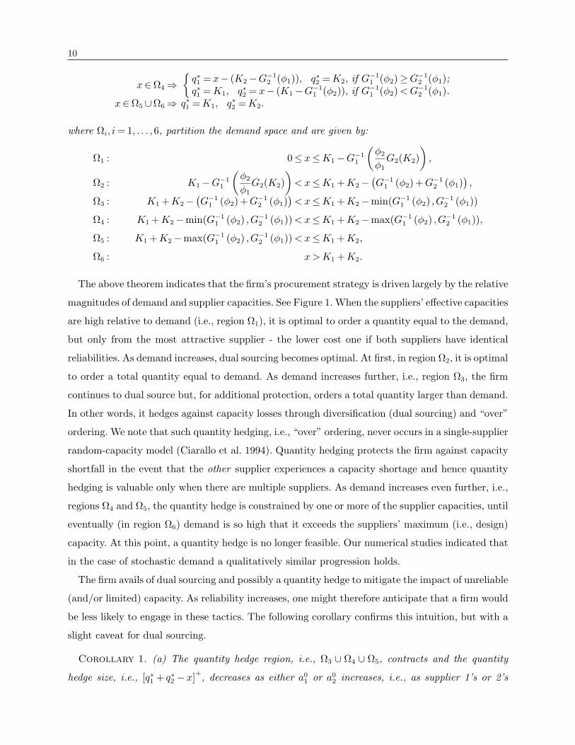
The above theorem indicates that the firm’s procurement strategy is driven largely by the relative
magnitudes of demand and supplier capacities. See Figure 1. When the suppliers’ effective capacities
are high relative to demand (i.e., region Ω1), it is optimal to order a quantity equal to the demand,
but only from the most attractive supplier - the lower cost one if both suppliers have identical
reliabilities. As demand increases, dual sourcing becomes optimal. At first, in region Ω2, it is optimal
to order a total quantity equal to demand. As demand increases further, i.e., region Ω3, the firm
continues to dual source but, for additional protection, orders a total quantity larger than demand.
In other words, it hedges against capacity losses through diversification (dual sourcing) and “over”
ordering. We note that such quantity hedging, i.e., “over” ordering, never occurs in a single-supplier
random-capacity model (Ciarallo et al. 1994). Quantity hedging protects the firm against capacity
shortfall in the event that the other supplier experiences a capacity shortage and hence quantity
hedging is valuable only when there are multiple suppliers. As demand increases even further, i.e.,
regions Ω4 and Ω5, the quantity hedge is constrained by one or more of the supplier capacities, until
eventually (in region Ω6) demand is so high that it exceeds the suppliers’ maximum (i.e., design)
capacity. At this point, a quantity hedge is no longer feasible. Our numerical studies indicated that
in the case of stochastic demand a qualitatively similar progression holds.
The firm avails of dual sourcing and possibly a quantity hedge to mitigate the impact of unreliable
(and/or limited) capacity. As reliability increases, one might therefore anticipate that a firm would
be less likely to engage in these tactics. The following corollary confirms this intuition, but with a
slight caveat for dual sourcing.
Corollary 1. (a) The quantity hedge region, i.e., Ω3 ∪ Ω4 ∪ Ω5, contracts and the quantity
hedge size, i.e., [q∗1 + q∗2 −x]+, decreases as either a01 or a0
2 increases, i.e., as supplier 1’s or 2’s

11
Qua
ntity
Hed
ge
Sin
gle
Sourc
e
Dual S
ourc
e
1 2 3 4 5 6
21 KK
xDemand
* 2
* 1quan
tity
tP
rocu
rem
enq
q
Figure 1 Optimal procurement quantity as a function of demand
reliability increases. (b) The single sourcing region, i.e., Ω1, expands as a01 increases and contracts
as a02 increases.
While the quantity hedge becomes less attractive as either supplier’s reliability increases4, dual
sourcing may become more attractive if the (initially) non-preferred supplier’s reliability increases
sufficiently to compensate for its cost and/or reliability disadvantage. If both suppliers are initially
identical, then dual sourcing becomes less attractive as either supplier’s reliability increases.
4.2. Single Sourcing With Improvement
In the pure improvement strategy the firm can source from only one supplier. Because improvement
efforts are not guaranteed to succeed, the firm may wish to delay commitment to a supplier until
after observing the success or failure of its improvement efforts. We call this late commitment.
Alternatively, the firm may commit to a supplier before observing the improvement outcome. We
call this early commitment. Both early and late commitment are observed in practice. “Interviews
with purchasing managers ... indicated that supplier development is not always successful. If the
effort fails the supplier may be dropped despite the fact that the buying firm has invested in
the supplier,” Krause (1999) p.219. However, “performance improvement sought by buying firms
4 The fact [q∗1 + q∗2 −x]+ decreases as reliability increases should not be confused with Lemma 2(a) which states thatq∗i increases in supplier i’s reliability. Recall that Lemma 1 implies that an increase in q1 results in a decrease in q2
(and vice versa), and so the total order quantity q∗1 + q∗2 can decrease in the reliability.
12
are often only possible when they commit to long-term relationships with key suppliers,” Krause
et al. (2007) p.531, and so some firms prefer to commit to the supplier in advance, e.g., the diesel-
engine manufacturer Varity Corp. (Handfield et al. 2000). In what follows, we first consider early
commitment and then late commitment.
4.2.1. Early Commitment The firm selects one supplier and (after making improvement
efforts) single sources from that supplier. For the moment, let i denote the chosen supplier. After
characterizing the optimal improvement effort, we will discuss supplier selection.
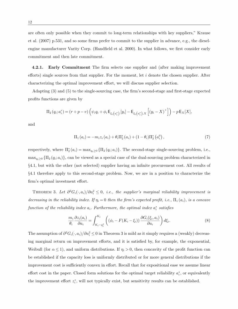
Adapting (3) and (5) to the single-sourcing case, the firm’s second-stage and first-stage expected
profits functions are given by
Π2 (qi;ari ) = (r + p− v)
(ψiqi +φi Eξi(ar
i ) [yi]−Eξi(ari ),X
[(yi−X)+
])− pEX [X],
and
Π1 (ai) =−mizi (ai)+ θiΠ∗2 (ai)+ (1− θi)Π∗
2
(a0
i
), (7)
respectively, where Π∗2 (ai) = maxqi≥0 Π2 (qi;ai). The second-stage single-sourcing problem, i.e.,
maxqi≥0 Π2 (qi;ai), can be viewed as a special case of the dual-sourcing problem characterized in
§4.1, but with the other (not selected) supplier having an infinite procurement cost. All results of
§4.1 therefore apply to this second-stage problem. Now, we are in a position to characterize the
firm’s optimal investment effort.
Theorem 3. Let ∂2Gi(·, ai)/∂a2i ≤ 0, i.e., the supplier’s marginal reliability improvement is
decreasing in the reliability index. If ηi = 0 then the firm’s expected profit, i.e., Π1 (ai), is a concave
function of the reliability index ai. Furthermore, the optimal index a∗i satisfies
mi
θi
∂zi(ai)∂ai
=∫ Ki
Ki−q∗i
((φi−F (Ki− ξi))
∂Gi(ξi, ai)∂ai
)dξi. (8)
The assumption of ∂2Gi(·, ai)/∂a2i ≤ 0 in Theorem 3 is mild as it simply requires a (weakly) decreas-
ing marginal return on improvement efforts, and it is satisfied by, for example, the exponential,
Weibull (for α≤ 1), and uniform distributions. If ηi > 0, then concavity of the profit function can
be established if the capacity loss is uniformly distributed or for more general distributions if the
improvement cost is sufficiently convex in effort. Recall that for expositional ease we assume linear
effort cost in the paper. Closed form solutions for the optimal target reliability a∗i , or equivalently
the improvement effort z∗i , will not typically exist, but sensitivity results can be established.
13
Corollary 2. The firm’s optimal improvement effort z∗i is (a) decreasing in the improvement
cost mi, (b) increasing in the improvement success probability θi, (c) decreasing in the unit pro-
curement cost ci, (d) increasing in the committed cost ηi, and (e) increasing in the unit revenue
r.
To this point, we have characterized the optimal improvement effort if the firm selects supplier
i = 1,2 as its single source. The question remains as to which supplier, 1 or 2, the firm should select.
Numerically, this is readily solved by comparing the optimal expected profit associated with each
supplier. Analytically, we can establish some properties of the optimal selection. In what follows,
we first establish that the potential for reliability improvement can influence supplier selection but
only if the two suppliers differ in more than one dimension. We then investigate supplier selection
when suppliers differ in both cost and reliability.
Let i∗ denote the firm’s preferred supplier if reliability improvement is possible and let j∗ denote
the firm’s preferred supplier if reliability improvement is not possible.
Theorem 4. (a) If suppliers 1 and 2 differ in at most one attribute, then i∗ = j∗. (b) If suppliers
1 and 2 differ in more than one attribute, then i∗ may not equal j∗.
The second result is important from a supplier’s perspective: willingness to collaborate on improve-
ment can be an order winner even if the supplier is less competitive on other dimensions.
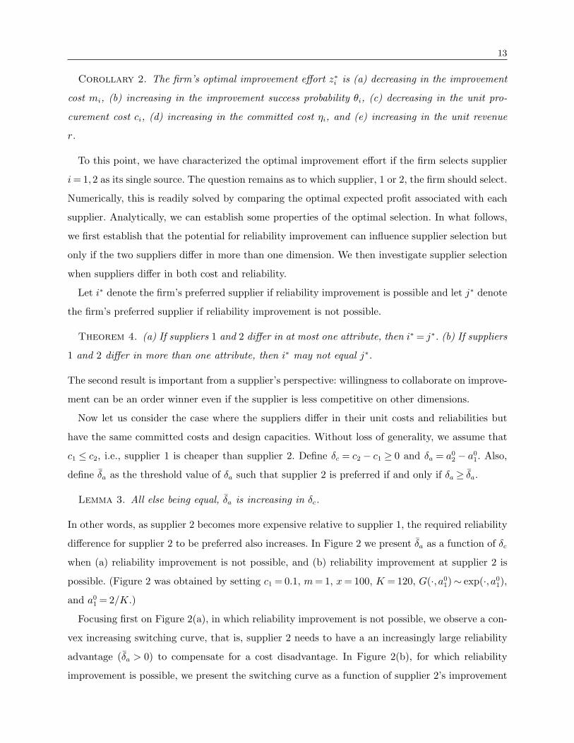
Now let us consider the case where the suppliers differ in their unit costs and reliabilities but
have the same committed costs and design capacities. Without loss of generality, we assume that
c1 ≤ c2, i.e., supplier 1 is cheaper than supplier 2. Define δc = c2 − c1 ≥ 0 and δa = a02 − a0
1. Also,
define δa as the threshold value of δa such that supplier 2 is preferred if and only if δa ≥ δa.
Lemma 3. All else being equal, δa is increasing in δc.
In other words, as supplier 2 becomes more expensive relative to supplier 1, the required reliability
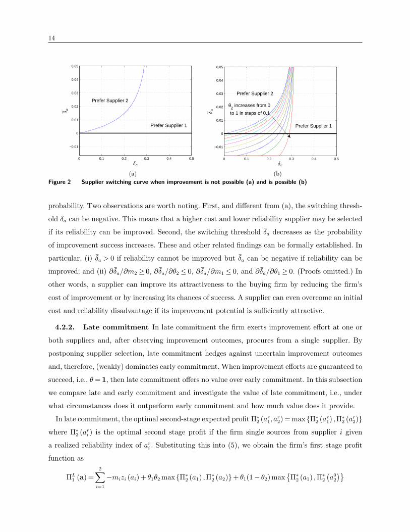
difference for supplier 2 to be preferred also increases. In Figure 2 we present δa as a function of δc
when (a) reliability improvement is not possible, and (b) reliability improvement at supplier 2 is
possible. (Figure 2 was obtained by setting c1 = 0.1, m = 1, x = 100, K = 120, G(·, a01)∼ exp(·, a0
1),
and a01 = 2/K.)
Focusing first on Figure 2(a), in which reliability improvement is not possible, we observe a con-
vex increasing switching curve, that is, supplier 2 needs to have a an increasingly large reliability
advantage (δa > 0) to compensate for a cost disadvantage. In Figure 2(b), for which reliability
improvement is possible, we present the switching curve as a function of supplier 2’s improvement
14
0 0.1 0.2 0.3 0.4 0.5
−0.01
0
0.01
0.02
0.03
0.04
0.05
δc
δa
Prefer Supplier 2
Prefer Supplier 1
(a)
0 0.1 0.2 0.3 0.4 0.5
−0.01
0
0.01
0.02
0.03
0.04
0.05
δc
δa
Prefer Supplier 1
Prefer Supplier 2
θ2 increases from 0
to 1 in steps of 0.1
(b)
Figure 2 Supplier switching curve when improvement is not possible (a) and is possible (b)
probability. Two observations are worth noting. First, and different from (a), the switching thresh-
old δa can be negative. This means that a higher cost and lower reliability supplier may be selected
if its reliability can be improved. Second, the switching threshold δa decreases as the probability
of improvement success increases. These and other related findings can be formally established. In
particular, (i) δa > 0 if reliability cannot be improved but δa can be negative if reliability can be
improved; and (ii) ∂δa/∂m2 ≥ 0, ∂δa/∂θ2 ≤ 0, ∂δa/∂m1 ≤ 0, and ∂δa/∂θ1 ≥ 0. (Proofs omitted.) In
other words, a supplier can improve its attractiveness to the buying firm by reducing the firm’s
cost of improvement or by increasing its chances of success. A supplier can even overcome an initial
cost and reliability disadvantage if its improvement potential is sufficiently attractive.
4.2.2. Late commitment In late commitment the firm exerts improvement effort at one or
both suppliers and, after observing improvement outcomes, procures from a single supplier. By
postponing supplier selection, late commitment hedges against uncertain improvement outcomes
and, therefore, (weakly) dominates early commitment. When improvement efforts are guaranteed to
succeed, i.e., θ = 1, then late commitment offers no value over early commitment. In this subsection
we compare late and early commitment and investigate the value of late commitment, i.e., under
what circumstances does it outperform early commitment and how much value does it provide.
In late commitment, the optimal second-stage expected profit Π∗2 (ar
1, ar2) = maxΠ∗
2 (ar1) ,Π∗
2 (ar2)
where Π∗2 (ar
i ) is the optimal second stage profit if the firm single sources from supplier i given
a realized reliability index of ari . Substituting this into (5), we obtain the firm’s first stage profit
function as
ΠL1 (a) =
2∑i=1
−mizi (ai)+ θ1θ2 maxΠ∗2 (a1) ,Π∗
2 (a2)+ θ1(1− θ2)maxΠ∗
2 (a1) ,Π∗2
(a0
2
)
15
+(1− θ1)θ2 maxΠ∗
2
(a0
1
),Π∗
2 (a2)
+(1− θ1)(1− θ2)maxΠ∗
2
(a0
1
),Π∗
2
(a0
2
), (9)
where we use the superscript L to denote that it is the late-commitment profit function. Because
of the max operation in (9), ΠL1 (a) is neither concave nor unimodal in a.
Let a∗Li denote the optimal reliability index for supplier i = 1,2 in late commitment and a∗Ei
denote the optimal reliability index if supplier i = 1,2 is selected in early commitment.
Lemma 4. a∗Li ≤ a∗Ei for i = 1,2
Late commitment targets a (weakly) lower reliability index for a supplier than does early com-
mitment assuming that supplier is selected in early commitment. Equivalently, the firm exerts
(weakly) less effort on improving a supplier. The reason is that in late commitment a particular
supplier, say i, is used if and only if it is preferred in the second stage, whereas in early commit-
ment that supplier (if selected) is guaranteed to be used in the second stage. The uncertainty as
to whether a supplier will be used dampens the firm’s improvement effort.
We now turn our attention to the value provided by late commitment. We use Π∗L1 (Π∗E
1 ) to
denote the optimal late (early) commitment expected profit. Letting j denote the complement of
i, i.e., j = 2(1) if i = 1(2), it follows (almost immediately) from Lemma 4 and (9), that Π∗L1 = Π∗E
1
if Π∗2 (a∗Ei ) < Π∗
2
(a0
j
)for i = 1 or i = 2. That is, late commitment offers no value if one supplier
dominates the other in the sense that the supplier (at its currently reliability) is preferred to the
other supplier at that supplier’s optimum (early commitment) reliability. If such a dominance
exists, there is no value to postponing supplier selection as the optimal selection does not depend
on improvement outcomes. In absence of this dominance, late commitment can provide value.
Theorem 5. Let suppliers 1 and 2 be identical except for their unit costs and let c1 ≤ c2. Then
Π∗L1 > Π∗E
1 if [Π∗2 (a∗E2 )−Π∗
2 (a01)]
+>
mz(a∗E2 )
θ(1−θ).
Corollary 3. (a) If Π∗L1 > Π∗E
1 for some c1 = c1 ≤ c2, then Π∗L1 > Π∗E
1 for all c1 ≤ c1 ≤ c2. (b)
There exists θa and θb with 0 < θa < θb < 1 such that Π∗L1 = Π∗E
1 if θ < θa or θ > θb.
Theorem 5 and its corollary tell us that cost difference, improvement success probability, and
improvement cost all play a role in determining whether late commitment outperforms early com-
mitment. Let us take each in turn. As the difference in unit costs c2 − c1 decreases, the more
expensive supplier requires a smaller reliability advantage to be selected in the second stage (this
follows from Lemma 3). Therefore, the firm is less certain (in the first stage) as to which supplier
will be preferred, and so there is more value in postponing its selection. A similar argument holds
for any supplier parameter: the more similar the suppliers are the more value there is to postponing
16
selection. Late commitment is less likely to offer value when the improvement success probability
θ is very low or very high. By allowing for improvement effort at both suppliers, late commitment
hedges against an improvement failure at one supplier. This hedging benefit is more pronounced
if the probability of one success and one failure is high, as that is the event in which the hedge
is useful. Thus, the hedging benefit is low if θ is very low (very high) because the probability of
both efforts failing (succeeding) is high. As the unit improvement cost m increases, the cost of
experimentation (i.e., improve one or both suppliers before choosing which is best) increases and,
therefore, one might reasonably conjecture that the value of late commitment should decrease in
the improvement cost. We did observe this in our numerical study.
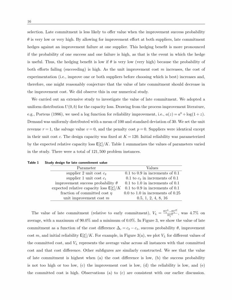
We carried out an extensive study to investigate the value of late commitment. We adopted a
uniform distribution U(0, b) for the capacity loss. Drawing from the process improvement literature,
e.g., Porteus (1986), we used a log function for reliability improvement, i.e., a(z) = a0 +log(1+ z).
Demand was uniformly distributed with a mean of 100 and standard deviation of 30. We set the unit
revenue r = 1, the salvage value v = 0, and the penalty cost p = 0. Suppliers were identical except
in their unit cost c. The design capacity was fixed at K = 120. Initial reliability was parameterized
by the expected relative capacity loss E[ξ]/K. Table 1 summarizes the values of parameters varied
in the study. There were a total of 121,500 problem instances.
Table 1 Study design for late commitment value
Parameter Valuessupplier 2 unit cost c2 0.1 to 0.9 in increments of 0.1supplier 1 unit cost c1 0.1 to c2 in increments of 0.1
improvement success probability θ 0.1 to 1.0 in increments of 0.1expected relative capacity loss E[ξ]/K 0.1 to 0.9 in increments of 0.1
fraction of committed cost η 0.0 to 1.0 in increments of 0.25unit improvement cost m 0.5, 1, 2, 4, 8, 16
The value of late commitment (relative to early commitment), VL = Π∗L1 −Π∗E
1
Π∗E1
, was 4.7% on
average, with a maximum of 90.0% and a minimum of 0.0%. In Figure 3, we show the value of late
commitment as a function of the cost difference ∆c = c2 − c1, success probability θ, improvement
cost m, and initial reliability E[ξ]/K. For example, in Figure 3(a), we plot VL for different values of
the committed cost, and VL represents the average value across all instances with that committed
cost and that cost difference. Other subfigures are similarly constructed. We see that the value
of late commitment is highest when (a) the cost difference is low, (b) the success probability
is not too high or too low, (c) the improvement cost is low, (d) the reliability is low, and (e)
the committed cost is high. Observations (a) to (c) are consistent with our earlier discussion.

17
That is, late commitment is valuable when suppliers are similar, hedging benefits are high, and
experimentation cost is low. In addition, late commitment is more valuable when suppliers are more
unreliable and the committed cost is high. At higher committed costs η, the firm is more sensitive
to low reliability because it incurs a higher cost for undelivered units. Therefore, late commitment
is more valuable as η increases because late commitment gives a higher probability of at least one
supplier having increased reliability.
0 0.2 0.4 0.6 0.8 10%
3%
6%
9%
12%
15%
18%
(b) improvement success probability θ
0 5 10 150%
3%
6%
9%
12%
15%
18%
(c) unit improvement cost m
VL, V
alue
of l
ate
com
mitm
ent
0 0.2 0.4 0.6 0.8 10%
3%
6%
9%
12%
15%
18%
(d) E[ξ]/K(→ decreasing reliability)
0 0.2 0.4 0.6 0.80%
3%
6%
9%
12%
15%
18%
(a) cost difference ∆c
VL, V
alue
of l
ate
com
mitm
ent
η decreases (1:−0.25:0)
η decreases (1:−0.25:0)
η decreases (1:−0.25:0)
η decreases (1:−0.25:0)
Figure 3 The value of late commitment
5. Dual Sourcing or Single Sourcing with Improvement?
Having investigated dual sourcing (DS) and single sourcing with improvement (SSI), we now explore
how attributes of the suppliers, e.g., cost and reliability, influence the firm’s preference for DS or
SSI. Define Π∗SSI and Π∗
DS as the optimal expected profit for the SSI and DS strategies, respectively.
(We do not consider any fixed costs associated with a given strategy as the directional effects of
such fixed costs are obvious.) Before comparing the strategies, we take a brief detour that will be
helpful for interpreting some later findings.
18
The fundamental challenge in a random-supply setting is that the delivered quantity can differ
from the ordered quantity. For the purposes of this discussion, consider any general supply process
that transforms an order q into a delivery y (q). Let us define ρ (q) = y (q)/q as the “yield” for
a given order quantity q. The buying firm faces two challenges: a mean effect and a variability
effect. The mean effect refers to the fact that E [ρ (q)]≤ 1.5 Absent variability, i.e., when ρ (q) is a
deterministic function of q, then the firm can scale its order quantity to ensure it receives exactly
the quantity it desires. However, if the firm faces a positive committed cost, then this scaling can
be expensive as the firm pays for units not received. The variability effect refers to the fact that the
firm is uncertain about the quantity it will receive. This uncertainty results in the firm having to
deal with overage or underage costs even if demand is deterministic. For a deterministic demand,
random yield model with no committed cost, Agrawal and Nahmias (1997) prove that the buying
firm is better off when the mean yield is higher and the yield variance is lower. While it may not be
generally true that variance fully captures the variability effect, it is helpful to frame our discussion
of DS and SSI in terms of how each strategy influences the mean and variance of ρ (q), denoted
as µρ (q) and σ2ρ (q) respectively. In a random capacity setting, both DS and SSI increase µρ (q)
(proof omitted) and reduce σ2ρ (q) (numerically observed) relative to the “original” single supplier
system and, therefore, improve the firm’s performance by mitigating the mean/variability effects
of random capacity.6 DS achieves this by splitting the order between suppliers, whereas SSI does
it by reducing (in a stochastic sense) the supplier’s capacity loss. For later use, we note that if the
two suppliers have identically distributed effective capacities, then the more the order split departs
from an equal division, the less mitigation benefit DS achieves.
5.1. Nonidentical Suppliers
Firms within a given industry may exhibit heterogeneity in their capabilities and performance
due to (among other things) “their history or initial firm endowment,” Barney (2001) p.647, or
their geographic location (Hazra and Mahadevan 2006). Arguing that the internet has facilitated
global sourcing, Hazra and Mahadevan (2006) suggest that supply base heterogeneity has increased
in recent years and that supplier capacity and cost structures are two primary dimensions of
heterogeneity. In this paper, we say that two suppliers are more heterogeneous if they differ more
on a particular attribute. For example, define c1 = c − ∆c and c2 = c + ∆c, then the suppliers
5 In theory a random supply process may result in E [ρ (q)] > 1 but it is natural to consider E [ρ (q)] ≤ 1. The logicpresented can be adapted to the case in which E [ρ (q)] > 1.
6 In comparing DS to the original single-supplier system which is limited to q ≤ K, it is appropriate to comparethe mean and variability for q ≤K. In this case DS increases the mean and reduces the variability. For q > K, DSincreases the mean but may increase the variability because the single source supply system can provide at most K.

19
become more heterogeneous as ∆c increases (0≤∆c < c). We refer to ∆c as the cost heterogeneity
parameter. Analogously to ∆c, define ∆η, ∆a, and ∆K as the committed cost, reliability, and
capacity heterogeneity parameters, respectively.
Theorem 6. Assuming both suppliers are identical except in the pertinent heterogeneity param-
eter, then (a) Π∗SSI is increasing in ∆c, ∆K, ∆η and ∆a, (b) Π∗
DS is increasing in ∆c and ∆η.
Also, Π∗DS is increasing in ∆a if G(·, a) is uniformly distributed.7
One supplier becomes more attractive and one becomes less so as the heterogeneity parame-
ter increases. Being a single-sourcing strategy, SSI benefits as heterogeneity increases because its
preferred supplier becomes more attractive. That DS should benefit from heterogeneity is less obvi-
ous as there is a tension between the increasing attractiveness of one supplier and the decreasing
attractiveness of the other. Focusing on the unit cost, the firm can reduce its average unit cost by
directing more of its order to the lower cost supplier but doing so reduces the mean/variabilility
mitigation benefit associated with dual sourcing. However, the average cost benefit outweighs the
mitigation disadvantage. A similar argument holds for the committed cost.8
More interesting, perhaps, than the effect of supplier heterogeneity on strategy performance is
its effect on strategy preference. We examine this question both numerically and analytically. We
constructed 18,750 base case instances for the study. The underlying study was the same as that
described in §4.2.2 but with the base case parameter values in this study described in Table 2.
For each base case, we studied the impact of heterogeneity in cost, reliability, design capacity, and
committed cost. For each heterogeneity type, we did the following for all 18,750 base case instances:
we created eleven different heterogeneity values (for example, varying the ratio of ∆c/c from 0%
to maximum possible values min(99%, r/c− 1)) and solved for the optimal dual and improvement
strategies at each heterogeneity value.9 For any given heterogeneity value, let %SSI denote the %
of base cases in which SSI was strictly preferred, i.e., Π∗SSI > Π∗
DS. Define %DS similarly and define
%Ind as the % of cases in which the firm was indifferent, i.e., Π∗SSI = Π∗
DS. For each heterogeneity
type, Figure 4 presents %SSI, %DS and %Ind as a function of the pertinent heterogeneity value.
We discuss each heterogeneity type in turn.
7 Recall that for a uniform (0, b) distribution, the reliability index a is given by 1/b. Numerically, we observed thatΠ∗DS was increasing in ∆a even if G(·, a) follows some other types of distributions, e.g., the Weibull distribution.Numerically we observed that Π∗DS was also increasing in ∆K .
8 If supplier 1 and supplier 2 differ in more than one parameter, then increasing heterogeneity can hurt dual sourcingeven if increasing heterogeneity makes supplier 1 unambiguously more attractive and supplier 2 unambiguously lessattractive. Examples available from authors.
9 When exploring committed cost heterogeneity, we excluded the η = 0 and η = 1 cases as we cannot have heterogeneityabout these extreme values.
20
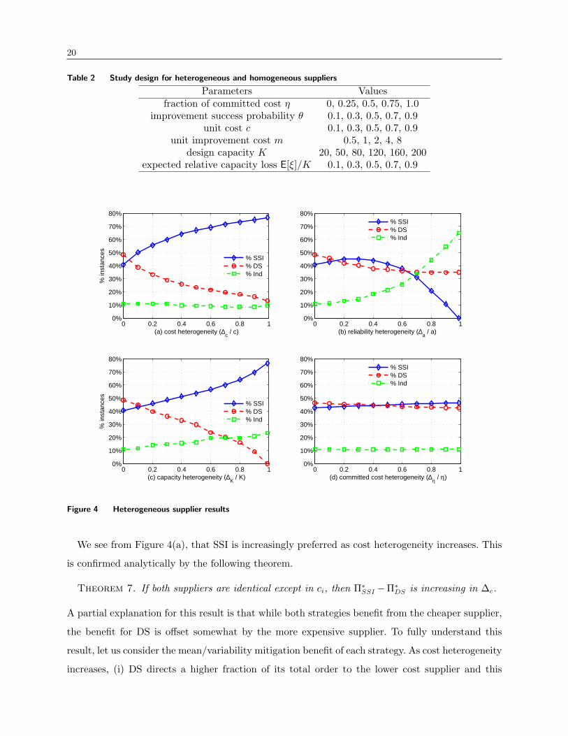
Table 2 Study design for heterogeneous and homogeneous suppliers
Parameters Valuesfraction of committed cost η 0, 0.25, 0.5, 0.75, 1.0
improvement success probability θ 0.1, 0.3, 0.5, 0.7, 0.9unit cost c 0.1, 0.3, 0.5, 0.7, 0.9
unit improvement cost m 0.5, 1, 2, 4, 8design capacity K 20, 50, 80, 120, 160, 200
expected relative capacity loss E[ξ]/K 0.1, 0.3, 0.5, 0.7, 0.9
0 0.2 0.4 0.6 0.8 10%
10%
20%
30%
40%
50%
60%
70%
80%
(b) reliability heterogeneity (∆a / a)
0 0.2 0.4 0.6 0.8 10%
10%
20%
30%
40%
50%
60%
70%
80%
(c) capacity heterogeneity (∆K / K)
% in
stan
ces
0 0.2 0.4 0.6 0.8 10%
10%
20%
30%
40%
50%
60%
70%
80%
(d) committed cost heterogeneity (∆η / η)
0 0.2 0.4 0.6 0.8 10%
10%
20%
30%
40%
50%
60%
70%
80%
(a) cost heterogeneity (∆c / c)
% in
stan
ces
% SSI% DS% Ind
% SSI% DS% Ind
% SSI% DS% Ind
% SSI% DS% Ind
Figure 4 Heterogeneous supplier results
We see from Figure 4(a), that SSI is increasingly preferred as cost heterogeneity increases. This
is confirmed analytically by the following theorem.
Theorem 7. If both suppliers are identical except in ci, then Π∗SSI −Π∗
DS is increasing in ∆c.
A partial explanation for this result is that while both strategies benefit from the cheaper supplier,
the benefit for DS is offset somewhat by the more expensive supplier. To fully understand this
result, let us consider the mean/variability mitigation benefit of each strategy. As cost heterogeneity
increases, (i) DS directs a higher fraction of its total order to the lower cost supplier and this
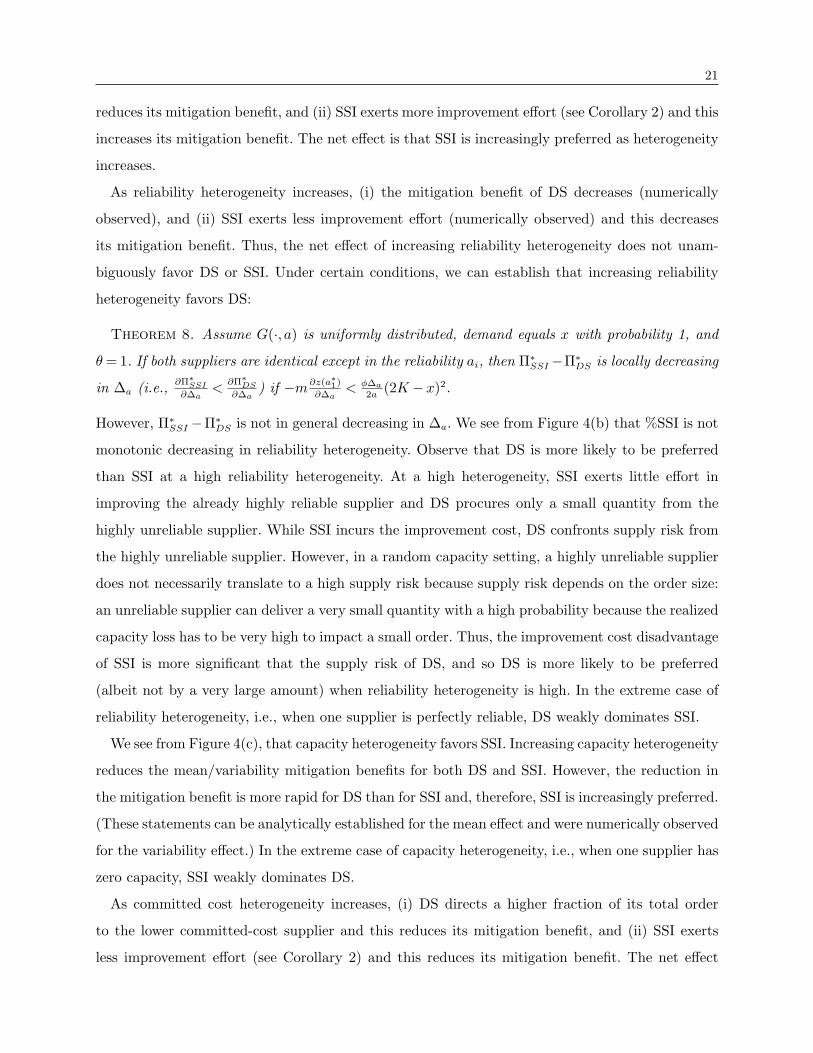
21
reduces its mitigation benefit, and (ii) SSI exerts more improvement effort (see Corollary 2) and this
increases its mitigation benefit. The net effect is that SSI is increasingly preferred as heterogeneity
increases.
As reliability heterogeneity increases, (i) the mitigation benefit of DS decreases (numerically
observed), and (ii) SSI exerts less improvement effort (numerically observed) and this decreases
its mitigation benefit. Thus, the net effect of increasing reliability heterogeneity does not unam-
biguously favor DS or SSI. Under certain conditions, we can establish that increasing reliability
heterogeneity favors DS:
Theorem 8. Assume G(·, a) is uniformly distributed, demand equals x with probability 1, and
θ = 1. If both suppliers are identical except in the reliability ai, then Π∗SSI−Π∗
DS is locally decreasing
in ∆a (i.e., ∂Π∗SSI∂∆a
<∂Π∗DS∂∆a
) if −m∂z(a∗1)
∂∆a< φ∆a
2a(2K −x)2.
However, Π∗SSI −Π∗
DS is not in general decreasing in ∆a. We see from Figure 4(b) that %SSI is not
monotonic decreasing in reliability heterogeneity. Observe that DS is more likely to be preferred
than SSI at a high reliability heterogeneity. At a high heterogeneity, SSI exerts little effort in
improving the already highly reliable supplier and DS procures only a small quantity from the
highly unreliable supplier. While SSI incurs the improvement cost, DS confronts supply risk from
the highly unreliable supplier. However, in a random capacity setting, a highly unreliable supplier
does not necessarily translate to a high supply risk because supply risk depends on the order size:
an unreliable supplier can deliver a very small quantity with a high probability because the realized
capacity loss has to be very high to impact a small order. Thus, the improvement cost disadvantage
of SSI is more significant that the supply risk of DS, and so DS is more likely to be preferred
(albeit not by a very large amount) when reliability heterogeneity is high. In the extreme case of
reliability heterogeneity, i.e., when one supplier is perfectly reliable, DS weakly dominates SSI.
We see from Figure 4(c), that capacity heterogeneity favors SSI. Increasing capacity heterogeneity
reduces the mean/variability mitigation benefits for both DS and SSI. However, the reduction in
the mitigation benefit is more rapid for DS than for SSI and, therefore, SSI is increasingly preferred.
(These statements can be analytically established for the mean effect and were numerically observed
for the variability effect.) In the extreme case of capacity heterogeneity, i.e., when one supplier has
zero capacity, SSI weakly dominates DS.
As committed cost heterogeneity increases, (i) DS directs a higher fraction of its total order
to the lower committed-cost supplier and this reduces its mitigation benefit, and (ii) SSI exerts
less improvement effort (see Corollary 2) and this reduces its mitigation benefit. The net effect
22
is therefore unclear. We see from Figure 4(d) that committed cost heterogeneity has only a weak
effect but that SSI seems to be increasingly preferred as heterogeneity increases.
To this point we have assumed that suppliers differed only on a single dimension and so increasing
heterogeneity made one supplier unambiguously better. When suppliers differ on multiple dimen-
sions, increasing heterogeneity may not favor one supplier. For example, cost and reliability may
be negatively correlated: as the cost difference increases so does the reliability difference with the
lower cost supplier becoming less reliable. In our numerical studies, we observed that cost hetero-
geneity (which favors SSI) had a stronger effect than reliability heterogeneity (which favors DS at
high heterogeneity).
5.2. Identical suppliers
We now explore how supplier attributes influence the firm’s strategy preference (DS or SSI) assum-
ing a homogenous (i.e., identical) supply base. That is, we investigate if and how the firm’s pref-
erence changes as a particular attribute, e.g., supplier cost, is changed simultaneously for both
suppliers. For example, both suppliers might be impacted by increases in energy prices and pass
this price increase on to the firm. As we assume suppliers are identical in this subsection we sup-
press the supplier subscript i = 1,2 on parameters. Π∗SSI increases in the success probability θ and
decreases in the improvement cost m. Therefore, all else being equal, SSI is favored as θ increases
or m decreases. Both Π∗SSI and Π∗
DS decrease in the cost c and committed cost η but increase in the
design capacity K and reliability index a. We conducted a numerical study to explore the impact
on strategy preference. The underlying study was the same as used in the heterogeneous study (see
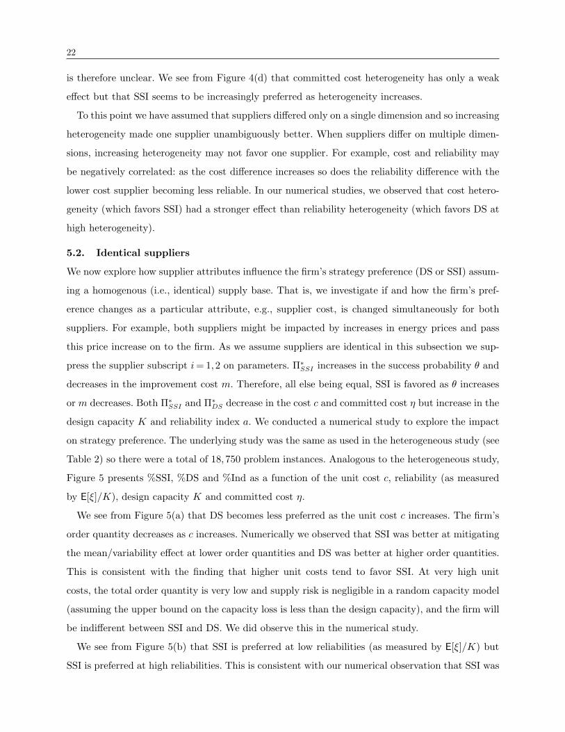
Table 2) so there were a total of 18,750 problem instances. Analogous to the heterogeneous study,
Figure 5 presents %SSI, %DS and %Ind as a function of the unit cost c, reliability (as measured
by E[ξ]/K), design capacity K and committed cost η.
We see from Figure 5(a) that DS becomes less preferred as the unit cost c increases. The firm’s
order quantity decreases as c increases. Numerically we observed that SSI was better at mitigating
the mean/variability effect at lower order quantities and DS was better at higher order quantities.
This is consistent with the finding that higher unit costs tend to favor SSI. At very high unit
costs, the total order quantity is very low and supply risk is negligible in a random capacity model
(assuming the upper bound on the capacity loss is less than the design capacity), and the firm will
be indifferent between SSI and DS. We did observe this in the numerical study.
We see from Figure 5(b) that SSI is preferred at low reliabilities (as measured by E[ξ]/K) but
SSI is preferred at high reliabilities. This is consistent with our numerical observation that SSI was

23
0 0.2 0.4 0.6 0.8 10%
10%
20%
30%
40%
50%
60%
70%
80%
90%
(b) E[ξ]/K (→ decreasing reliability)
0 50 100 150 2000%
10%
20%
30%
40%
50%
60%
70%
80%
90%
(c) design capacity K
% in
stan
ces
0 0.2 0.4 0.6 0.8 10%
10%
20%
30%
40%
50%
60%
70%
80%
90%
(d) committed cost η
0 0.2 0.4 0.6 0.8 10%
10%
20%
30%
40%
50%
60%
70%
80%
90%
(a) unit cost c
% in
stan
ces
% SSI% DS% Ind
% SSI% DS% Ind
% SSI% DS% Ind
% SSI% DS% Ind
Figure 5 Homogenous supplier results
better at mitigating the mean/variability effect at lower reliabilities and DS was better at higher
reliabilities.
We see from Figure 5(c) that the preference for DS decreases as the design capacity increases.
If E[ξ]/K < 0.5, supply risk decreases as K increases as there is an increasingly large guaranteed
minimum capacity. The firm is then indifferent between DS and SSI for sufficiently high K. If
E[ξ]/K ≥ 0.5, supply risk does not disappear even at very high capacities and SSI is weakly preferred
to DS.
We see from Figure 5(d) that SSI is increasingly preferred as the committed cost η increases.
SSI exerts more improvement effort as η increase (see Corollary 2) and this increases its mitigation
benefit. One mechanism DS uses to manages supply risk is the quantity hedge but this is more
expensive as the committed cost increases. The combined effect is to make SSI increasingly preferred
as η increases.
24
6. Combined Strategy
As discussed in §1, some firms, e.g., Honda and Toyota, engage in both dual sourcing and process
improvement, and we now turn our attention to the general problem in which the firm can com-
bine improvement (of one or both suppliers) with dual sourcing. The following lemma partially
characterizes the firm’s expected profit function, Π1 (a), which was given earlier by (5).
Lemma 5. Π1 (a) is a submodular function in a.
Although Π1 (a) can be component-wise unimodal in its reliability index a, it is not in general
jointly concave.
Our primary objective is to explore the value of deploying a combined strategy. We denote the
optimal expected profit for the combined strategy as Π∗COM . Recall that Π∗
DS and Π∗SSI denote the
optimal expected profits for the pure strategies, dual source and single-source with improvement,
and so Π∗COM ≥maxΠ∗
SSI ,Π∗DS. We define Ψ = (Π∗
COM −maxΠ∗SSI ,Π∗
DS)/maxΠ∗SSI ,Π∗
DS as
the value of the combined strategy, i.e., Ψ is the relative increase in expected profit as compared
to the best (for the given problem instance) of the pure strategies. Unless otherwise stated, Π∗SSI
refers to the early commitment optimal profit. We numerically investigated the value of the com-
bined strategy. Because the experimentation/hedging benefit of the late commitment strategy is
embedded in the combined strategy, and this value is highest when suppliers are identical (§4.2.2),
we focused on identical suppliers in our study. As suppliers become less similar, the value of the
combined strategy will decrease. The underlying study was the same as used in §5 (see Table 2)
and so there were 18,750 problem instances.
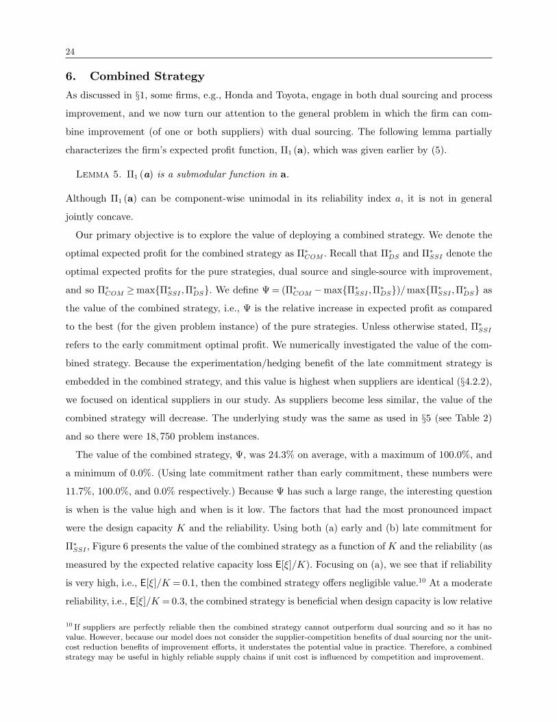
The value of the combined strategy, Ψ, was 24.3% on average, with a maximum of 100.0%, and
a minimum of 0.0%. (Using late commitment rather than early commitment, these numbers were
11.7%, 100.0%, and 0.0% respectively.) Because Ψ has such a large range, the interesting question
is when is the value high and when is it low. The factors that had the most pronounced impact
were the design capacity K and the reliability. Using both (a) early and (b) late commitment for
Π∗SSI , Figure 6 presents the value of the combined strategy as a function of K and the reliability (as
measured by the expected relative capacity loss E[ξ]/K). Focusing on (a), we see that if reliability
is very high, i.e., E[ξ]/K = 0.1, then the combined strategy offers negligible value.10 At a moderate
reliability, i.e., E[ξ]/K = 0.3, the combined strategy is beneficial when design capacity is low relative
10 If suppliers are perfectly reliable then the combined strategy cannot outperform dual sourcing and so it has novalue. However, because our model does not consider the supplier-competition benefits of dual sourcing nor the unit-cost reduction benefits of improvement efforts, it understates the potential value in practice. Therefore, a combinedstrategy may be useful in highly reliable supply chains if unit cost is influenced by competition and improvement.

25
to mean demand (which was set to 100 in this study). In this case, the buying firm wants to
access as much effective capacity as possible and therefore wants to dual source and improve both
suppliers. At lower reliabilities, i.e., E[ξ]/K = 0.5,0.7,0.9, the combined strategy retains value even
at design capacities that are twice the mean demand. Focusing on (b), we see a qualitatively similar
finding but with a lower value for combined strategy because late commitment dominates early
commitment.
0 50 100 150 2000%
10%
20%
30%
40%
50%
60%
70%
80%
90%
(a) design capacity K
Ψ, V
alue
of c
ombi
ned
stra
tegy
0 50 100 150 2000%
10%
20%
30%
40%
50%
60%
70%
80%
90%
(b) design capacity K
early commitment late commitment
E[ξ]/K decreasing(0.9 → 0.1)
E[ξ]/K decreasing(0.9 → 0.1)
Figure 6 The value of the combined strategy
In both the dual sourcing and combined strategies, the firm can, but does not have to, source
from both suppliers. When suppliers are identical, Theorem 2 and Corollary 1 imply that the
firm will source from both suppliers at one pair of reliabilities if it does so at any pair of higher
reliabilities. Therefore, if suppliers are identical, the combined strategy sources from both suppliers
only if the dual sourcing strategy does. In our study, dual sourcing used both suppliers in 88.7%
of the instances and the combined strategy did so in 71.1% of instances.
7. Random Yield
We now consider random-yield type of supply uncertainty and adopt the commonly-used model
in which the delivered quantity is stochastically proportional to the order quantity, i.e., yi =
minqi, ξiqi, where ξi now represents supplier-i’s yield rather than its capacity loss.11 The random
yield version of our model is identical to that formulated in §3 but with yi = minqi, ξiqi replacing
11 ξi has a nonnegative support. If the support has an upper bound of 1,yi = minqi, ξiqi can be written as yi = ξiqi.

26
yi = minqi, (Ki− ξi)+ and Gi(·, ai) now referring to the yield distribution (for a given reliability
index ai) rather than the capacity-loss distribution. A natural model of reliability improvement for
random yield is one in which the yield is (first-order) stochastically larger after improvement and,
therefore, an increase in the reliability index, say from ai to ai implies Gi(·, ai)≥Gi(·, ai). Using
this random yield model (hereafter RY), we replicated our earlier analysis of the random capacity
model (hereafter RC). We also replicated all our numerical studies.12 For the sake of brevity, we
focus our discussion here on the key results and, in particular, focus on some important differences
between RC and RY. Appendix B contains full statements and proofs of all theoretical results
referred to in this section.
In RC, both dual sourcing (DS) and single sourcing with improvement (SSI) mitigate the mean
and variability effects of supply risk. However, in RY, (i) DS mitigates the variability effect but
has no impact on the mean effect; and (ii) SSI mitigates the mean effect and (depending on the
yield distribution) may mitigate or amplify the variability effect (proofs omitted).13
Similar to RC, the RY dual-sourcing quantity problem is well-behaved. In fact the expected
profit is jointly concave in the order quantities if Gi has support over [0,1] (see Theorem 9) and
not simply jointly unimodal as for RC.14 Similar to RC, Π∗DS is increasing in a supplier’s reliability
index ai (Lemma 6). Different from RC, however, the quantity procured from a supplier is not
necessarily increasing, nor even monotonic, in ai, and can strictly decrease in ai (Lemma 7).
Similar to RC, the improvement problem is concave subject to certain restrictions (Theorem 10).
Different from RC, however, improvement effort can decrease as the unit cost decreases (Lemma 8).
With regard to late versus early commitment, the findings on the directional impact of improvement
cost, success probability, reliability, supplier cost difference, and committed cost were similar to
those for RC. The value of late commitment was, however, lower in RY, with an average value of
1.4% (compared to 4.7% for RC), a maximum of 87.0% and a minimum of 0.0%.
We next consider the impact of supplier heterogeneity in RY. As with RC, both Π∗DS and Π∗
SSI
increase in heterogeneity (Theorem 6). With regard to the impact of heterogeneity on strategy
12 Each study was the same as that described for the random capacity model except that we assumed a uniformlydistributed random yield rather than a uniformly distributed a capacity loss. The expected yield loss values, i.e.,1− E [ξ] were set to the same values as the expected relative capacity loss E[ξ]/K values in the random capacitystudies. As we did not want the design capacity constraint to obscure the comparison of RC and RY, in our numericalstudies we adopted a random yield model with a design capacity constraint of K, i.e., yi = minqi, ξiqi and qi ≤Ki.
13 SSI mitigates the variability effect if the yield has a uniform (a,1) distribution but amplifies the variability effectif the yield has a Weibull (α,β) distribution (in which case the reliability index is a = β).
14 Parlar and Wang (1993) established joint concavity for a dual-sourcing, random-yield newsvendor when the firmpays fully for the quantity ordered, i.e., η = 1. The joint-concavity result extends readily to the case of η≤ 1.
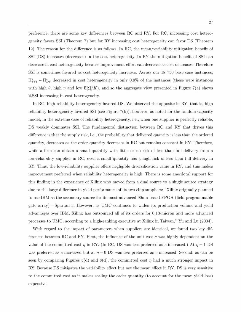
27
preference, there are some key differences between RC and RY. For RC, increasing cost hetero-
geneity favors SSI (Theorem 7) but for RY increasing cost heterogeneity can favor DS (Theorem
12). The reason for the difference is as follows. In RC, the mean/variability mitigation benefit of
SSI (DS) increases (decreases) in the cost heterogeneity. In RY the mitigation benefit of SSI can
decrease in cost heterogeneity because improvement effort can decrease as cost decreases. Therefore
SSI is sometimes favored as cost heterogeneity increases. Across our 18,750 base case instances,
Π∗SSI −Π∗
DS decreased in cost heterogeneity in only 0.9% of the instances (these were instances
with high θ, high η and low E[ξ]/K), and so the aggregate view presented in Figure 7(a) shows
%SSI increasing in cost heterogeneity.
In RC, high reliability heterogeneity favored DS. We observed the opposite in RY, that is, high
reliability heterogeneity favored SSI (see Figure 7(b)); however, as noted for the random capacity
model, in the extreme case of reliability heterogeneity, i.e., when one supplier is perfectly reliable,
DS weakly dominates SSI. The fundamental distinction between RC and RY that drives this
difference is that the supply risk, i.e., the probability that delivered quantity is less than the ordered
quantity, decreases as the order quantity decreases in RC but remains constant in RY. Therefore,
while a firm can obtain a small quantity with little or no risk of less than full delivery from a
low-reliability supplier in RC, even a small quantity has a high risk of less than full delivery in
RY. Thus, the low-reliability supplier offers negligible diversification value in RY, and this makes
improvement preferred when reliability heterogeneity is high. There is some anecdotal support for
this finding in the experience of Xilinx who moved from a dual source to a single source strategy
due to the large difference in yield performance of its two chip suppliers: “Xilinx originally planned
to use IBM as the secondary source for its most advanced 90nm-based FPGA (field programmable
gate array) - Spartan 3. However, as UMC continues to widen its production volume and yield
advantages over IBM, Xilinx has outsourced all of its orders for 0.13-micron and more advanced
processes to UMC, according to a high-ranking executive at Xilinx in Taiwan,” Yu and Lu (2004).
With regard to the impact of parameters when suppliers are identical, we found two key dif-
ferences between RC and RY. First, the influence of the unit cost c was highly dependent on the
value of the committed cost η in RY. (In RC, DS was less preferred as c increased.) At η = 1 DS
was preferred as c increased but at η = 0 DS was less preferred as c increased. Second, as can be
seen by comparing Figures 5(d) and 8(d), the committed cost η had a much stronger impact in
RY. Because DS mitigates the variability effect but not the mean effect in RY, DS is very sensitive
to the committed cost as it makes scaling the order quantity (to account for the mean yield loss)
expensive.

28
0 0.2 0.4 0.6 0.8 10%
10%
20%
30%
40%
50%
60%
70%
80%
(b) reliability heterogeneity (∆a / a)
0 0.2 0.4 0.6 0.8 10%
10%
20%
30%
40%
50%
60%
70%
80%
(c) capacity heterogeneity (∆K / K)
% in
stan
ces
0 0.2 0.4 0.6 0.8 10%
10%
20%
30%
40%
50%
60%
70%
80%
(d) committed cost heterogeneity (∆η / η)
0 0.2 0.4 0.6 0.8 10%
10%
20%
30%
40%
50%
60%
70%
80%
(a) cost heterogeneity (∆c / c)
% in
stan
ces
% SSI% DS% Ind
% SSI% DS% Ind
% SSI% DS% Ind
% SSI% DS% Ind
Figure 7 Heterogeneous supplier results
With regard to the value of the combined strategy in RY, the average value was 10.2% (as
compared to 24.3% for RC), with a maximum of 100.0% and a minimum of 0.0%. Using late
commitment, these numbers were 6.1%, 100.0% and 0.0% respectively. As with RC, the value of
combined strategy was highest when capacity and reliability were low. The two semiconductor
competitors Xilinx and Altera (who both deal with random-yield suppliers) offer an interesting
contrast in supplier strategies: “One place where Xilinx takes a distinctively different tack from
arch-rival Altera is in their foundry strategy. Xilinx uses multiple foundries - today Toshiba and
UMC – claiming that multiple foundries give a hedge against process problems and increase volume
production capability. Altera, on the other hand, claims that working with a single fab - TSMC –
gives them an edge because they can focus their engineering efforts on the capabilities and char-
acteristics of a single supplier, allowing them to converge faster on a high-yield, high-performance
design with each process generation,” (Morris 2006). The Xilinx strategy is consistent with our
findings that the combined strategy is valuable if capacity and reliability are a concern. Altera’s
view suggests that single sourcing might make improvement efforts more efficient (a perspective
not captured in our model) which would lower the value of a combined strategy.
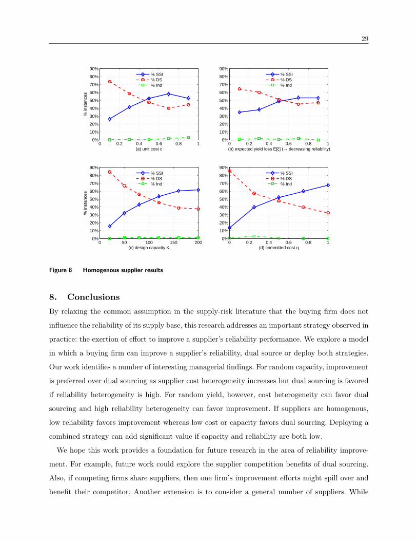
29
0 0.2 0.4 0.6 0.8 10%
10%
20%
30%
40%
50%
60%
70%
80%
90%
(b) expected yield loss E[ξ] (→ decreasing reliability)
0 50 100 150 2000%
10%
20%
30%
40%
50%
60%
70%
80%
90%
(c) design capacity K
% in
stan
ces
0 0.2 0.4 0.6 0.8 10%
10%
20%
30%
40%
50%
60%
70%
80%
90%
(d) committed cost η
0 0.2 0.4 0.6 0.8 10%
10%
20%
30%
40%
50%
60%
70%
80%
90%
(a) unit cost c
% in
stan
ces
% SSI% DS% Ind
% SSI% DS% Ind
% SSI% DS% Ind
% SSI% DS% Ind
Figure 8 Homogenous supplier results
8. Conclusions
By relaxing the common assumption in the supply-risk literature that the buying firm does not
influence the reliability of its supply base, this research addresses an important strategy observed in
practice: the exertion of effort to improve a supplier’s reliability performance. We explore a model
in which a buying firm can improve a supplier’s reliability, dual source or deploy both strategies.
Our work identifies a number of interesting managerial findings. For random capacity, improvement
is preferred over dual sourcing as supplier cost heterogeneity increases but dual sourcing is favored
if reliability heterogeneity is high. For random yield, however, cost heterogeneity can favor dual
sourcing and high reliability heterogeneity can favor improvement. If suppliers are homogenous,
low reliability favors improvement whereas low cost or capacity favors dual sourcing. Deploying a
combined strategy can add significant value if capacity and reliability are both low.
We hope this work provides a foundation for future research in the area of reliability improve-
ment. For example, future work could explore the supplier competition benefits of dual sourcing.
Also, if competing firms share suppliers, then one firm’s improvement efforts might spill over and
benefit their competitor. Another extension is to consider a general number of suppliers. While

30
there is anecdotal support for some of our findings, it would be of interest to empirically test
some of the observations to develop a richer understanding of supply risk strategies. We note that
because “most chip makers don’t speak publicly about yield problems” (Weil 2004), it might be
difficult to obtain data on supplier reliability performance.
Acknowledgements
The authors would like to thank the associate editor and the three referees for their comments and
suggestions, which significantly improved this paper.
ReferencesAgrawal, N., S. Nahmias. 1997. Rationalization of the supplier base in the presence of yield uncertainty.
Production and Operations Management 6 291–308.
Anupindi, Ravi, Ram Akella. 1993. Diversification under supply uncertainty. Management Science 39(8)
944–963.
Aydin, Goker, Evan L. Porteus. 2008. Joint inventory and pricing decisions for an assortment. Operations
Research 56(5) 1247–1255.
Babich, Volodymyr, Apostolos N. Burnetas, Peter H. Ritchken. 2007. Competition and diversification effects
in supply chains with supplier default risk. Manufacturing & Service Operations Management 9(2)
123–146.
Barney, J. B. 2001. Resource-based theories of competitive advantage: A ten-year retrospective on the
resource-based view. Journal of Management 27(6) 643–650.
Carrillo, Janice E., Cheryl Gaimon. 2000. Improving manufacturing performance through process change
and knowledge creation. Management Science 46(2) 265–288.
Carrillo, Janice E., Cheryl Gaimon. 2004. Managing knowledge-based resource capabilities under uncertainty.
Management Science 50(11) 1504–1518.
Chand, Suresh, Herbert Moskowitz, Andreas Novak, Ishpal Rekhi, Gerhard Sorger. 1996. Capacity allocation
for dynamic process improvement with quality and demand considerations. Operations Research 44(6)
964–975.
Ciarallo, F. W., R. Akella, T. E. Morton. 1994. A periodic review, production planning model with uncertain
capacity and uncertain demand: Optimality of extended myopic policies. Management Science 40(3)
320–332.
Dada, Maqbool, Richard Marcellus. 1994. Process control with learning. Operations Research 42(2) 323–336.
Dada, Maqbool, Nicholas C. Petruzzi, Leroy B. Schwarz. 2007. A newsvendor’s procurement problem when
suppliers are unreliable. Manufacturing & Service Operations Management 9(1) 9–32.
Erdem, Asli. 1999. Inventory models with random yield. Chapter 4, PhD dissertation .
31
Federgruen, Awi, Nan Yang. 2007a. Optimal supply diversification under general supply risks. Forthcoming.
Operations Research .
Federgruen, Awi, Nan Yang. 2007b. Quality competition under yield uncertainty. Working Paper. .
Fine, Charles H. 1986. Quality improvment and learning in productive systems. Management Science 32(10)
1301–1315.
Fine, Charles H., Evan L. Porteus. 1989. Dynamic process improvement. Operations Research 37(4) 580–591.
Gerchak, Yigal, Mahmut Parlar. 1990. Yield randomness, cost trade-offs and diversification in the EOQ
model. Naval Research Logistics 37 341–354.
Gurler, Ulku, Mahmut Parlar. 1997. An inventory problem with two randomly available suppliers. Operations
Research 45(6) 904–918.
Handfield, R.B., D.R. Krause, T.V. Scannell, R.M. Monczka. 2000. Avoid the pitfalls in supplier development.
Sloan Management Review 4 37–49.
Hazra, J., B. Mahadevan. 2006. Impact of supply base heterogeneity in electronic markets. European Journal
of Operational Research 174(3) 1580–1594.
Krause, Daniel R., Lisa M. Ellram. 1997. Critical elements of supplier development: The buying firm per-
spective. European Journal of Purchasing and Supply Management 3(1) 21–31.
Krause, D.R. 1997. Supplier development: Current practices and outcomes. Journal of Supply Chain Man-
agement 33(2) 12–19.
Krause, D.R. 1999. The antecedents of buying firms’ efforts to improve suppliers. Journal of Operations
Management 17(2) 205–224.
Krause, D.R., R.B. Handfield, T.V. Scannell. 1998. An empirical investigation of supplier development:
reactive and strategic processes. Journal of Operations Management 17(1) 39–58.
Krause, D.R., R.B. Handfield, B.B. Tyler. 2007. The relationships between supplier development, commit-
ment, social capital accumulation and performance improvement. Journal of Operations Management
25(2) 528–545.
Leenders, Michiel R., David L. Blenkhorn. 1988. Reverse Marketing . The Free Press.
Liker, Jeffrey K., Thomas Y. Choi. 2004. Building deep supplier relationships. Harvard Business Review
82(12) 104–113.
Liu, Shaoxuan, Kut C. So, Fuqiang Zhang. 2009. The effect of supply reliability in a retail setting with joint
marketing and inventory decisions (forthcoming). Manufacturing & Service Operations Management .
Marcellus, Richard L., Maqbool Dada. 1991. Interactive process quality improvement. Management Science
37(11) 1365–1376.
Morris, Kevin. 2006. Virtex-5 is alive - the high end gets higher. FPGA and Structured ASIC Journal
Http://www.fpgajournal.com/articles 2006/20060516 virtex.htm.
32
Parlar, Mahmut, David Perry. 1996. Inventory models of future supply uncertainty with single and multiple
suppliers. Naval Research Logistics 43 191–210.
Parlar, Mahmut, Dan Wang. 1993. Diversification under yield randomness in inventory models. European
Journal of Operational Research 66(1) 52–64.
Porteus, Evan L. 1986. Optimal lot sizing, process quality improvement and setup cost reduction. Operations
Research 34(1) 137–144.
SCQI. 2009. Supplier continuous quiality improvement (intel publicly available document).
https://supplier.intel.com/static/quality/SCQIHandbook.pdf .
Sheffi, Yossi. 2005. The Resilient Enterprise. The MIT Press.
Spence, Anne M., Evan L. Porteus. 1987. Setup reduction and increased effective capacity. Management
Science 33(10) 1291–1301.
Swaminathan, Jayashankar M., J. George Shanthikumar. 1999. Supplier diversification: effect of discrete
demand. Operations Research Letters 24(5) 213–221.
Swinney, R., S. Netessine. 2008. Long-term contracts under the threat of supplier default. Manufacturing &
Service Operations Management. Published online in Articles in Advance, January 25, 2008. .
Terwiesch, Christian, Roger E. Bohn. 2001. Learning and process improvement during production ramp-up.
Int. J. Production Economics 70 1–19.
Tomlin, Brian. 2006. On the value of mitigation and contingency strategies for managing supply-chain
disruption risks. Management Science 52(5) 639–657.
Tomlin, Brian, Yimin Wang. 2005. On the value of mix flexibility and dual sourcing in unreliable newsvendor
networks. Manufacturing and Service Operations Management 7(1) 37–57.
Weil, Nancy. 2004. IBM says corner turned on chip yield problems. Computer World Operating Systems
May 12.
Wouters, Marc, Ewout van Jarwaardea, Bianca Groena. 2007. Supplier development and cost management
in southeast asia-results from a field study. Journal of Purchasing and Supply Management 13(4)
228–244.
Yu, Samson, Jack Lu. 2004. Due to IBM’s slow ramp, Xilinx, Nvidia raise outsourcing to UMC, TSMC.
Digitimes Friday 13 February 2004.
Zangwill, Willard I., Paul B. Kantor. 1998. Toward a theory of continuous improvement and the learning
curve. Management Science 44(7) 910–920.
Zhu, Kaijie, Rachel Q. Zhang, Fugee Tsung. 2007. Pushing quality improvement along supply chains. Man-
agement Science 53(3) 421–436.
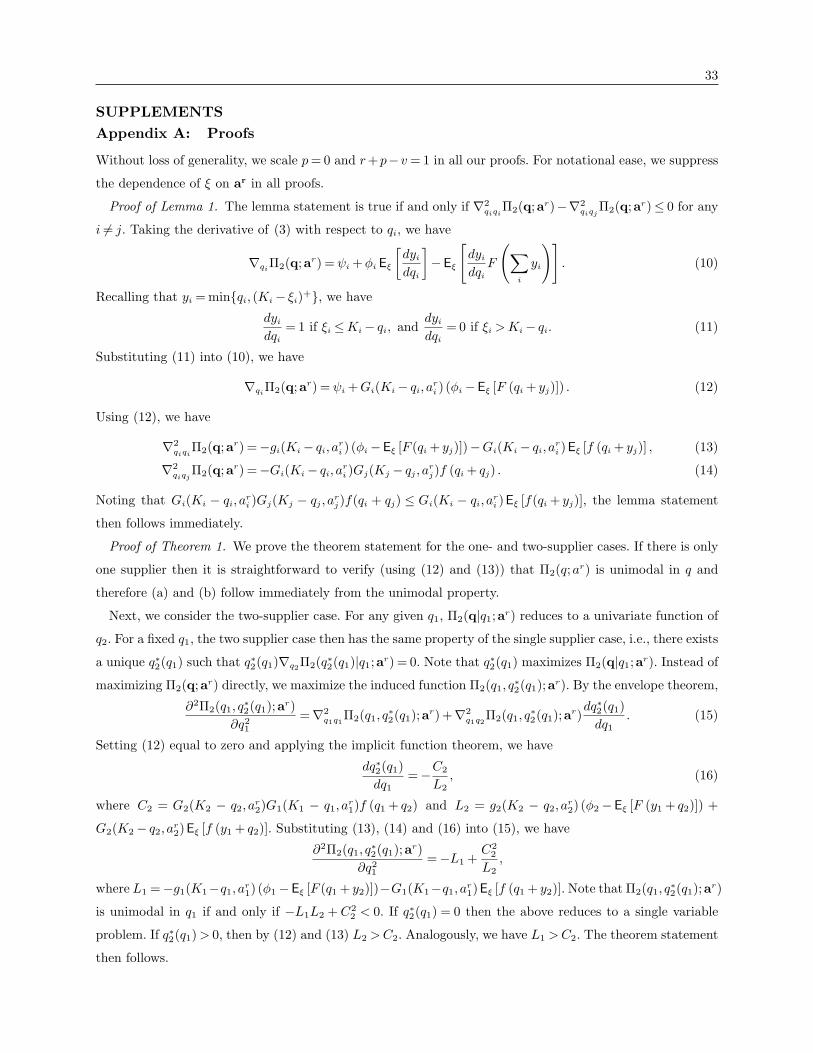
33
SUPPLEMENTSAppendix A: Proofs
Without loss of generality, we scale p = 0 and r +p−v = 1 in all our proofs. For notational ease, we suppress
the dependence of ξ on ar in all proofs.
Proof of Lemma 1. The lemma statement is true if and only if ∇2qiqi
Π2(q;ar)−∇2qiqj
Π2(q;ar)≤ 0 for any
i 6= j. Taking the derivative of (3) with respect to qi, we have
∇qiΠ2(q;ar) = ψi + φi Eξ
[dyi
dqi
]−Eξ
[dyi
dqi
F
(∑i
yi
)]. (10)
Recalling that yi = minqi, (Ki− ξi)+, we have
dyi
dqi
= 1 if ξi ≤Ki− qi, anddyi
dqi
= 0 if ξi > Ki− qi. (11)
Substituting (11) into (10), we have
∇qiΠ2(q;ar) = ψi + Gi(Ki− qi, a
ri ) (φi−Eξ [F (qi + yj)]) . (12)
Using (12), we have
∇2qiqi
Π2(q;ar) =−gi(Ki− qi, ari ) (φi−Eξ [F (qi + yj)])−Gi(Ki− qi, a
ri )Eξ [f (qi + yj)] , (13)
∇2qiqj
Π2(q;ar) =−Gi(Ki− qi, ari )Gj(Kj − qj , a
rj)f (qi + qj) . (14)
Noting that Gi(Ki − qi, ari )Gj(Kj − qj , a
rj)f(qi + qj) ≤ Gi(Ki − qi, a
ri )Eξ [f(qi + yj)], the lemma statement
then follows immediately.
Proof of Theorem 1. We prove the theorem statement for the one- and two-supplier cases. If there is only
one supplier then it is straightforward to verify (using (12) and (13)) that Π2(q;ar) is unimodal in q and
therefore (a) and (b) follow immediately from the unimodal property.
Next, we consider the two-supplier case. For any given q1, Π2(q|q1;ar) reduces to a univariate function of
q2. For a fixed q1, the two supplier case then has the same property of the single supplier case, i.e., there exists
a unique q∗2(q1) such that q∗2(q1)∇q2Π2(q∗2(q1)|q1;ar) = 0. Note that q∗2(q1) maximizes Π2(q|q1;ar). Instead of
maximizing Π2(q;ar) directly, we maximize the induced function Π2(q1, q∗2(q1);ar). By the envelope theorem,
∂2Π2(q1, q∗2(q1);ar)
∂q21
=∇2q1q1
Π2(q1, q∗2(q1);ar)+∇2
q1q2Π2(q1, q
∗2(q1);ar)
dq∗2(q1)dq1
. (15)
Setting (12) equal to zero and applying the implicit function theorem, we have
dq∗2(q1)dq1
=−C2
L2
, (16)
where C2 = G2(K2 − q2, ar2)G1(K1 − q1, a
r1)f (q1 + q2) and L2 = g2(K2 − q2, a
r2) (φ2−Eξ [F (y1 + q2)]) +
G2(K2− q2, ar2)Eξ [f (y1 + q2)]. Substituting (13), (14) and (16) into (15), we have
∂2Π2(q1, q∗2(q1);ar)
∂q21
=−L1 +C2
2
L2
,
where L1 =−g1(K1−q1, ar1) (φ1−Eξ [F (q1 + y2)])−G1(K1−q1, a
r1)Eξ [f (q1 + y2)]. Note that Π2(q1, q
∗2(q1);ar)
is unimodal in q1 if and only if −L1L2 + C22 < 0. If q∗2(q1) = 0 then the above reduces to a single variable
problem. If q∗2(q1) > 0, then by (12) and (13) L2 > C2. Analogously, we have L1 > C2. The theorem statement
then follows.
34
Proof of Lemma 2. Part a). Setting (12) equal to zero and applying the implicit function theorem, we
have
dq∗i (ari )
dari
=1|A|
∣∣∣∣∣− ∂hi
∂ai
∂hi
∂qj
− ∂hj
∂ai
∂hj
∂qj
∣∣∣∣∣ ,
where |A| denote the determinant of the hessian of Π2(q;ar) and hi and hj denote the first order derivatives
with respect to qi and qj , respectively. Using (12) to (14), one can verify that ∂hi/∂ari ≥ 0 and ∂hj/∂ar
i < 0.
Recognizing that |A|> 0 and all elements in A are negative, we have dq∗i (ari )/dar
i ≥ 0. Part b). Using (3), we
have
∂Π∗2(a
r)∂ar
i
= φi
dEξ[yi]dar
i
−∂ Eξ,X
[(∑
k yk −X)+]
∂ari
. (17)
One can show that
dEξ[yi]dar
i
=∫ Ki
Ki−q∗i
∂Gi(ξi, ari )
∂ari
dξi, and (18)
∂ Eξ,X
[(∑
k yk −X)+]
∂ari
= Eξ
[∫ Ki
Ki−q∗i
∂Gi(ξi, ari )
∂ari
F (Ki− ξi + yj)dξi
]. (19)
Substituting (18) and (19) into (17), we have
∂Π∗2(ar)
∂ari
= φi
∫ Ki
Ki−q∗i
∂Gi(ξi, ari )
∂ari
dξi−Eξ
[∫ Ki
Ki−q∗i
∂Gi(ξi, ari )
∂ari
F (Ki− ξi + yj)dξi
]
≥ φi
∫ Ki
Ki−q∗i
∂Gi(ξi, ari )
∂ari
dξi−Eξ
[∫ Ki
Ki−q∗i
∂Gi(ξi, ari )
∂ari
F (q∗i + yj)dξi
]
= φi
∫ Ki
Ki−q∗i
∂Gi(ξi, ari )
∂ari
dξi−Eξ [F (q∗i + yj)]∫ Ki
Ki−q∗i
∂Gi(ξi, ari )
∂ari
dξi
= (φi−Eξ [F (q∗i + yj)])∫ Ki
Ki−q∗i
∂Gi(ξi, ari )
∂ari
dξi ≥ 0. (20)
Note that (20) follows from the fact that ∂Gi(·, ari )/∂ar
i ≥ 0, and φi−Eξ [F (q∗i + yj)]≥ 0 by (12).
Proof of Theorem 2. Because η = 0, (6) can be simplified to
Gi(Ki− q∗i )(φi−Eξj
[F (qi + yj)])= 0, i = 1,2. (21)
To simplify notation we suppress the dependence on reliability and simply write Gi(·) = Gi(·, ai). We now
prove the theorem statement by considering different regions of the demand. First note that for any given
ε > 0, when q1 + q2 = x − ε both equations in (21) are strictly positive. We must have φ1G1(K1 − q1) =
φ2G2(K2− q2) unless φ1G1(K1−x)≥ φ2G2(K2)⇒ x≤K1−G−11
(φ2φ1
G2(K2)). Next consider the case when
q1 + q2 > x. Using (6), the optimal procurement quantity is given by
q∗1 = x− (K2−G−12 (φ1)), q∗2 = x− (K1−G−1
1 (φ2)). (22)
For q1 + q2 > x to hold, we must have x > K1 +K2−G−11 (φ2)−G−1
2 (φ1). However, for (22) to be an interior
solution, we must have φ1−G2(K2− (x−K1))≤ 0⇒ x≤K1 +K2−G−12 (φ1), and φ2−G1(K1− (x−K2))≤
0 ⇒ x ≤ K1 + K2 −G−11 (φ2). Therefore, we must have x ≤ K1 + K2 −min(G−1
1 (φ2),G−12 (φ1)) for firm to

35
dual source without hitting the capacity limit from one of the suppliers. Note that when the firm utilize the
fully capacity of one supplier, the total procurement quantity q∗1 + q∗2 > x. Otherwise, suppose q∗i < Ki and
q∗j = Kj (i = 1,2; j = 3− i), then we have q∗i + Kj = (x−Kj + G−1j (φi)) + Kj = x + G−1
j (φi) > x. The case of
both suppliers’ capacities are fully utilized can be similarly proved. The last region in the theorem statement
follows directly from the above analysis. Not all demand regions Ω1 to Ω6 exist for all parameter values. For
example, if the two suppliers are identical, then Ω1 will not exist. The optimal ordering quantity in each
region directly follows from the above analysis.
Proof of Corollary 1. (a) and (b) follow directly from Theorem 2 and fact that G−1i (·) decreases in ai.
Proof of Theorem 3. Using (7), we have
∂Π1(ai)∂ai
=−mi
dzi(ai)dai
+ θi
∂Π∗2(ai)
∂ai
, (23)
∂2Π1(ai)∂a2
i
=−mi
d2zi(ai)da2
i
+ θi
∂2Π∗2(ai)
∂a2i
, (24)
where
∂2Π∗2(ai)
∂a2i
=∂2Π2(qi;ai)
∂a2i
∣∣∣∣qi=q∗
i(ai)
+dq∗i (ai)
dai
∂2Π2(qi;ai)∂qi∂ai
∣∣∣∣qi=q∗
i(ai)
.
Note that by (12) ∂2Π2(qi;ai)
∂qi∂ai|qi=q∗
i(ai) = ∂Gi(Ki−q∗i ,ai)
∂ai(φi − F (q∗i )), which equals to 0 when ηi = 0 and q∗i
satisfies the first order condition (12). In addition,
d2zi(ai)da2
i
=− 1(a′i(z))2
a′′i (z)a′i(z)
. (25)
Substituting (25) and (20) into (24), and recalling that a′i(z)≥ 0 and a′′i (z)≤ 0, we have ∂2Π1(ai)/∂a2i ≤ 0.
Note that (8) can be obtained by setting (23) equal to zero.
Proof of Corollary 2. The corollary statements follow directly by applying the implicit function theorem
on (8).
Proof of Theorem 4. Part a. We prove the theorem statement by contradiction. If the two suppliers are
identical except for one parameter, the firm will always choose the more desirable supplier for its single-
sourcing supplier. Suppose c1 < c2 but the firm choose to make investment z∗ in supplier 2. Since the two
suppliers are identical except for this parameter, the optimal expected profit satisfies Π1(a∗2|c2) < Π1(a∗1|c1)
because ∂Π1(a∗)/∂c < 0. But this contradicts with the fact the firm find it optimal to invest in supplier
2. The theorem statement for other parameters can be analogously proved. Part b. We prove the theorem
statement by constructing a particular example. Assume demand X is deterministic, η = 0, and θ = 1.
Suppose suppliers 1 and 2 differ only in cost and reliability: i.e., c1 < c2 and a1 < a2 = ∞. Note that
φi Eξi[yi] = (r − ci)
∫ K
K−qiGi(ξ, ai)dξ. If improvement is not possible, the firm will choose to source from
supplier 2 if and only if
(r− c2)X > (r− c1)∫ K
K−X
G1(ξ, a1)dξ. (26)
Since X >∫ K
K−XG1(ξ, a1)dξ, it is easy to find parameter values such that c1 < c2 but (26) holds, i.e., the
firm sources from supplier 2. Now, if improvement is possible the firm will either source from supplier 2
36
or improve and source from supplier 1. Using (8), the optimal reliability after improvement is a1 = a01 +
r−c12m
∫ K
K−X
∂G1(ξ,a1)
∂a1dξ. Assume Gi(·, ai) is uniformly distributed with support greater than or equal to K, we
obtain a closed form solution as
a1 = a01 +
12m
12(r− c1)(K2− (K −X)2). (27)
Let ∆ denote the LHS - RHS of (26). If the optimal expected profit with supplier 1 is greater than ∆, then
the firm will source from supplier 1 (after improvement). Substituting (27) into (7), we have
Π1(a∗1) =− 14m1a2
1
[12(r− c1)(K2− (K −X)2)
]2
+[a1 +
12m1
12(r− c1)(K2− (K −X)2)
]× 1
2m1
12(r− c1)(K2− (K −X)2).
If Π1(a∗1) minus the RHS of (26) is greater than ∆, then the theorem statement is true. Note this can be
simplified to 12m1
(1− 1
2a21
)[12(r− c1)(K2− (K −X)2)
]2> ∆, which can be easily satisfied if a1 >
√2/2 and
m is small.
Proof of Lemma 3. Let Π1(a∗i ) denote the optimal expected profit associated with sourcing from supplier
i, where Π1(a∗i ) is given by (7). Let v = Π1(a∗2)−Π1(a∗1) = 0. By the implicit function theorem (IFT), we
have ∂δa/∂δc =−(∂v/∂δc)/(∂v/∂δa). By (7), ∂v/∂δc ≤ 0 and ∂v/∂δa ≥ 0. The lemma statement then follows.
Proof of Lemma 4. By (9), we have ∂ΠL1 (a)
∂ai= −mi
dzi(ai)
dai+ θiθj
∂∂ai
maxΠ∗2 (ai) ,Π∗
2 (aj) + θi(1 −θj) ∂
∂aimax
Π∗
2 (ai) ,Π∗2
(a0
j
). Because ∂
∂aiΠ∗
2 (aj) = 0 and ∂∂ai
Π∗2 (ai) ≥ 0 (Lemma 2), we have ∂ΠL
1 (a)
∂ai≤
−midzi(ai)
dai+ θiθj
∂∂ai
Π∗2 (ai) + θi(1− θj) ∂
∂aiΠ∗
2 (ai) = −midzi(ai)
dai+ θi
∂∂ai
Π∗2 (ai) = ∂ΠE
1 (a)
∂ai. Therefore, because
ΠE1 (a) is decreasing in ai for all ai > a∗E
i , ΠL1 (a) is also decreasing in ai for all ai > a∗E
i . Thus, a∗Li ≤ a∗E
i .
Proof of Theorem 5. Supplier 1 is the optimal selection for early commitment15 and
Π∗E1 =−mz
(a∗E1
)+ θΠ∗
2
(a∗E1
)+(1− θ)Π∗
2
(a01
). (28)
Π∗L1 ≥ΠL
1 (a∗E) because a∗E is a feasible improvement vector for late commitment. Now,
ΠL1
(a∗E
)=
2∑i=1
−mizi
(a∗E
i
)+ θ1θ2 max
Π∗
2
(a∗E1
),Π∗
2
(a∗E2
)+ θ1(1− θ2)max
Π∗
2
(a∗E1
),Π∗
2
(a02
)
+(1− θ1)θ2 maxΠ∗
2
(a01
),Π∗
2
(a∗E2
)+(1− θ1)(1− θ2)max
Π∗
2
(a01
),Π∗
2
(a02
).
Using the fact that suppliers are identical except that c1 < c2, we have Π∗2 (a∗E
1 ) > Π∗2 (a∗E
2 ) and Π∗2 (a∗E
1 ) >
Π∗2 (a0
2). Substituting these into ΠL1 (a∗E), we have,
ΠL1
(a∗E
)=−mz
(a∗E1
)−mz(a∗E2
)+ θΠ∗
2
(a∗E1
)
+ (1− θ)θmaxΠ∗
2
(a01
),Π∗
2
(a∗E2
)+(1− θ)2Π∗
2
(a01
). (29)
Comparing (28) and (29) and rearranging terms, Π∗L1 > Π∗E
1 if [Π∗2 (a∗E
2 )−Π∗2 (a0
1)]+
>mz(a∗2)
θ(1−θ).
15 Although suppliers are identical except for c, to aid exposition in the proof we keep the i subscript on the initialreliability index a0
1 even though a01 = a0
2. The subscript indicates which supplier is selected in the second stage.

37
Proof of Corollary 3. (a) follows from Theorem 5 and fact that Π∗2 (a0
1) is decreasing in c1 while Π∗2 (a∗E
2 )
and z (a∗2) are constant in c1. (b) follows from Theorem 5 and fact that [Π∗2 (a∗E
2 )−Π∗2 (a0
1)]+ is finite while
mz(a∗2)
θ(1−θ)→∞ as θ→ 0 or θ→ 1.
Proof of Theorem 6. We prove the theorem statement for the unit procurement cost. The theorem state-
ments associated with other system parameters can be analogously proved. First consider part (a). Because
suppliers are identical except for the unit procurement cost c, the improvement strategy selects the cheaper
supplier (c −∆c) and we label this supplier as supplier 1. We need the following property to prove the
theorem statement.
Property: ∂Π∗2(a
r)/∂∆c is increasing in ar1.
Proof: By Lemma 2, dq∗1/dar1 ≥ 0. By Lemma 1, Π2(q;ar) is a submodular function in q. It follows that
∂q∗2/∂ar1 ≤ 0. (Note this can also be directly verified by applying the implicit function theorem to (10).)
Using (1) and substituting c1 = c−∆c and c2 = c + ∆c, we have
∂Π∗2(a
r)∂∆c
= η(q∗1 − q∗2)+ (1− η) (Eξ1 [y1]−Eξ2 [y2]) . (30)
From above, dq∗1/dar1 ≥ 0 and dq∗2/dar
1 ≤ 0. Also, Eξ1 [y1] is increasing in ar1 and Eξ2 [y2] is constant in ar
1. We
therefore have ∂Π∗2(a
r)/∂∆c is increasing in ar1.
We are now in a position to prove the theorem statement. Note that
∂Π∗SSI
∂∆c
= θ∂Π∗
2(a1)∂∆c
+ (1− θ)∂Π∗
2(a01)
∂∆c
≥ ∂Π∗2(a
01)
∂∆c
= ηq∗1 +(1− η)Eξ[y1]≥ 0,
where the inequality follows from the above property. Part (b) of the theorem can be similarly proved by
noting that ∂Π∗DS/∂∆c equals ∂Π∗
2(ar)/∂∆c, which is non-negative as established above.
Proof of Theorem 7. We prove the theorem statement by leveraging results in Theorem 6. Consistent with
the proof of Theorem 6, we label the cheaper supplier (c−∆c) as supplier 1.
∂Π∗SSI
∂∆c
= θ∂Π∗
2(a1)∂∆c
+(1− θ)∂Π∗
2(a01)
∂∆c
≥ ∂Π∗2(a0
1)∂∆c
= ηq∗1 + (1− η)Eξ[y1]
≥ η(q∗1 − q∗2)+ (1− η) (Eξ[y1]−Eξ[y2]) =∂Π∗
DS
∂∆c
,
where the first inequality follows from the property proved in Theorem 6, i.e., ∂Π∗2(a1)/∂∆c is increasing in
a1.
Proof of Theorem 8. Recall that for the improvement strategy, the objective function is Π∗SSI = ΠSSI(a∗1) =
−mz(a∗1) + θΠ∗2(a
∗1)+ (1− θ)Π∗
2(a01). Hence, by the envelope theorem we have
∂Π∗SSI
∂∆a
=∂ΠSSI(a∗1)
∂a01
=−m∂z(a∗1)∂a0
1
+(1− θ)∂Π∗
2(a01)
∂a01
=−m∂z(a∗1)∂a0
1
,
where the last step follows from the assumption that θ = 1. Note that because capacity loss is uniformly
distributed, ΠSSI(a1) is inherently concave in a1 and therefore a∗1 is upper bounded. For reasonable forms of
improvement function z(a1),∂z(a∗1)
∂a01
is also bounded above. For the dual sourcing strategy, derivative of the
objective function with respect to ∆a is
∂Π∗DS
∂∆a
=∂Π∗
2(a01, a
02)
∂a01
− ∂Π∗2(a
01, a
02)
∂a02
.

38
Note that by Theorem 2, the firm will not use quantity hedge when demand satisfies x≤K1+K2−(G−11 (φ2)+
G−12 (φ1)). Note that although Theorem 2 assumes η = 0, this will not affect our analysis here since a positive
η only serves to reduce the optimal order quantity. Since the two suppliers are identical except for reliability,
we simply assume x < 2K.
∂Π∗DS
∂∆a
= φ
(q∗1
∂G(K − q∗1, a01)
∂a01
+∫ K
K−q∗1
(K − ξ)∂g(ξ, a0
1)∂a0
1
−q∗2∂G(K − q∗2, a
02)
∂a02
−∫ K
K−q∗2
(K − ξ)∂g(ξ, a0
2)∂a0
2
).
Substituting the uniform distribution U(0,1/a) into the above expression, we can simplify it to
∂Π∗DS
∂∆a
=φ
2(2K −x)(q∗1 − q∗2) > 0, (31)
where the inequality follows from the fact that x < 2K and q∗1 > q∗2. By Theorem 3, we know that q∗2
satisfies φ1G1(K1− (x− q∗2)) = φ2G2(K2− q∗2). Utilizing the uniform distribution, we can explicitly solve q∗2:
q∗2 = (a+∆a)x−2∆aK
2a. It follows that q∗1 = x− q∗2 = (a−∆a)x+2∆aK
2a. Substituting q∗1 and q∗2 into (31), we have
∂Π∗DS
∂∆a
=φ∆a
2a(2K −x)2 > 0,
Therefore, if −m∂z(a∗1)
∂a01
< φ∆a
2a(2K−x)2, then Π∗
SSI −Π∗DS decreases in ∆a. Note that the above condition is
valid since ∂z(a∗1)
∂a01
is bounded. The above condition is more likely to hold when m is small, K is large, (and
θ is large), and ∆a is large.
Proof of Lemma 5. Using (20), we have
∂2Π∗2(ar)
∂ai∂aj
=−∇ajEξ
[∫ Ki
Ki−q∗i
∂Gi(ξi, ai)∂ai
F (Ki− ξi + yj)dξi
]+
dq∗i (aj)daj
∂2Π∗2(ar)
∂ai∂qi
+dy∗j (aj)
daj
∂2Π∗2(ar)
∂ai∂yj
=−∫ Kj
Kj−q∗j
∫ Ki
Ki−q∗i
∂Gj(ξj , aj)∂aj
∂Gi(ξi, ai)∂ai
f (Ki− ξi + Kj − ξj)dξidξj
+dq∗i (aj)
daj
∂Gi(Ki− q∗i , ai)∂ai
(φi−Eξ F (qi + yj))
− dy∗j (aj)daj
∫ Ki
Ki−q∗i
∂Gi(ξi, ai)∂ai
∫ Kj−q∗j
0
f(Ki− ξi + qj)dGj(ξj , aj)dξi. (32)
Note that the first term in (32) is non-positive because ∂Gi(·, ai)/∂ai ≥ 0. The second term is non-positive
because dq∗i (aj)/daj ≤ 0 (by Lemma 1 and Lemma 2(a)), and the third term is non-positive because
dy∗j (aj)/daj ≥ 0. The lemma statement follows because ∂2Π1(a)/∂ai∂aj is a positive, linear combination of
∂2Π∗2(a
r)/∂ai∂aj .
Appendix B: Random Yield - Theorem Statements and Proofs
In this appendix we present the analytical results referenced in the main paper and the associated proofs.
B.1. Dual Sourcing
Theorem 9. If the random yield distribution Gi is bounded by 1, then the firm’s expected second-stage
profit, Π2(q;ar), is jointly concave in q.
39
Proof. Adapting (3) to the random yield model, we have
∂Π2(q;ar)∂qi
= ψi +φi
dEξ[yi]dqi
−∂ Eξ,X
[(∑
k yk −X)+]
∂qi
. (33)
Note that dEξ[yi]/dqi =∫ 1
0ξidGi(ξi, a
ri ), and ∂ Eξ,X
[(∑
k yk −X)+]/∂qi =
∫ 1
0ξi Eξ F (ξiqi + yj)dGi(ξi, a
ri ).
Substituting these two expressions into (33), we have
∂Π2(q;ar)∂qi
= ψi +∫ 1
0
ξi(φi−Eξ F (ξiqi + yj))dGi(ξi, ari ), i = 1,2. (34)
The second order derivatives with respect to q are therefore given by ∂2Π2(q;ar)/∂q2i =−∫ 1
0
∫ 1
0ξ2
i f(ξiqi +
ξjqj))dGj(ξj , arj)dGi(ξi, a
ri ), and ∂2Π2(q;ar)/∂qi∂qj = −∫ 1
0
∫ 1
0ξiξjf(ξiqi + ξjqj))dGj(ξj , a
rj)dGi(ξi, a
ri ).
Clearly, the Hessian is symmetric and all elements are negative. By Proposition 2 of Parlar and Wang (1993),
the determinant of the Hessian is non-negative. The lemma statement then follows.
Lemma 6. If the random yield distribution Gi(ξi, ari ) satisfies ∂Gi(ξi, a
ri )/∂ar
i =−ρξigi(ξi, ari ), where ρ is
a real, non-negative scaler, then the firm’s optimal expected second-stage profit, Π∗2(a
ri ), is increasing in the
supplier’s reliability index ari .
The assumption that ∂Gi(ξi, ari )/∂ar
i = −ρξigi(ξi, ari ) is a mild one, as it is satisfied by many common
distributions such as uniform u(0, a), exponential, and Weibull distributions.
Proof. Adapting (3) to the random yield model, we have
∂Π∗2(ar)
∂ari
= φi
dEξ[yi]dar
i
−∂ Eξ,X
[(∑
k yk −X)+]
∂ari
. (35)
Note that Eξ[yi] =∫ 1
0ξiq
∗i dGi(ξi, a
ri )+ (1−Gi(1, ar
i ))q∗i = q∗i
(1− ∫ 1
0Gi(ξi, a
ri )dξi
). It follows that
dEξ[yi]dar
i
=−q∗i
∫ 1
0
∂Gi(ξi, ari )
∂ari
dξi. (36)
For the second term in (35), note that Eξ,X
[(∑
k yk −X)+]
= Eξ
[(1−Gi(1, ar
i ))∫ q∗i +yj
0(q∗i + yj −x)dF (x)+
∫ 1
0
∫ ξiq∗i +yj
0(ξiq
∗i + yj −x)dF (x)dGi(ξi, a
ri )
], which can be simplified to Eξ
∫ q∗i +yj
0(q∗i + yj − x)dF (x) −
Eξ
∫ 1
0Gi(ξi, a
ri )q
∗i F (ξiq
∗i + yj)dξi. It follows that
∂ Eξ,X
[(∑
k yk −X)+]
∂ari
=−Eξ
[∫ 1
0
∂Gi(ξi, ari )
∂ari
q∗i F (ξiq∗i + yj)dξi
]. (37)
Substituting (36) and (37) into (35), we have
∂Π∗2(a
r)∂ar
i
=−φiq∗i
∫ 1
0
∂Gi(ξi, ari )
∂ari
dξi + Eξ
[∫ 1
0
∂Gi(ξi, ari )
∂ari
q∗i F (ξiq∗i + yj)dξi
]
=−q∗i
∫ 1
0
∂Gi(ξi, ari )
∂ari
[φi−Eξ F (ξiq∗i + yj)]dξi
= ρq∗i
∫ 1
0
ξigi(ξi, ari ) [φi−Eξ F (ξiq
∗i + yj)]dξi ≥ 0. (38)
Note that (38) follows from the assumption that ∂Gi(·, ari )/∂ar
i = −ρξigi(ξi, ari ), and
∫ 1
0ξi[φi −
Eξ F (ξiq∗i + yj)]dGi(ξi, a
ri )≥ 0 by the fact that q∗i satisfies the first order condition (see (34)). We note that
if ηi = 0 then (38) equals to 0, suggesting that in a random yield model, a higher reliability offers no value
when the firm pays only for what is delivered.
40
Lemma 7. For a single supplier case, if (a) Gi(ξi, ari ) ∼ U(ar
i ,1) and ψi +∫ 1
ariξi(φi − F ( ξi
ariF−1(φi +
ψi
ari)))dGi(ξi, a
ri )≤ 0, or (b) Gi(ξi, a
ri )∼U(0, ar
i ) and ψi +∫ ar
i
0ξi(φi−F ( ξi
ariF−1(φi + ψi
ari)))dGi(ξi, a
ri )≥ 0, then
∂q∗i /∂ari ≤ 0.
Note that the condition in part (a) is guaranteed to hold, for example, when ηi = 0. The condition in part
(b) is satisfied, for example, when ψi
ari
+φi ≤ 0 (e.g., when the unit cost ci is high). In addition, if demand is
deterministic, then dq∗i /dari ≤ 0 (see Lemma 8).
Proof. Part (a). By (34), the optimal procurement quantity q∗i satisfies
v = ψi +∫ 1
ari
ξigi(ξi, ari )(φi−F (ξiq
∗i ))dξi = 0. (39)
Applying the IFT to (39), we have dq∗i /dari =−(∂v/∂ar
i )/(∂v/∂qi). By concavity of Π2(q;ar), ∂v/∂qi ≤ 0. The
lemma statement is true if ∂v/∂ari ≤ 0. Note that ∂v/∂ar
i =∫ 1
ariξi
∂gi(ξi,ari )
∂ari
(φi−F (ξiq∗i ))dξi−ar
i gi(ari , a
ri )(φi−
F (ari q∗i )) =− 1
1−ari(ψi +ar
i (φi−F (ari qi))), which is negative if q∗i ≤ 1
ariF−1(φi + ψi
ari). Substituting this expres-
sion into (39) obtains the stated condition stated in part (a). Part (b). The proof is analogous to part (a)
and therefore is omitted.
B.2. Single Sourcing with Improvement
Theorem 10. (i) Let γ = 1 − 2(1 − ai)ψi − (1 − a2i )φi. If demand is deterministic and (a) Gi(·, ai) ∼
U(ai,1) and (√
γ − γ)2 ≥ (1 − ai)2(ψi + aiφi)2, or (b) Gi(·, ai) ∼ U(0, ai), then Π1 (ai) is concave in the
reliability index ai. Furthermore, the optimal index a∗i satisfies
mi
θi
dzi(ai)dai
=
12φiq
∗i − (q∗i −x)2
2(1−ai)2q∗i, if Gi(·, ai)∼U(ai,1);
12(φi− 1)q∗i + x2
2a2iq∗
i, if Gi(·, ai)∼U(0, ai).
(40)
(ii) If η = 0 and Gi(ξi, ari ) satisfies ∂Gi(ξi, a
ri )/∂ar
i = −ρξigi(ξi, ari ), where ρ is a real, non-negative scaler,
then the firm’s optimal expected profit Π1 (ai) is constant in the reliability index ai.
Proof. Part (i) First we note that both (24) and (25) in Theorem 3 apply to the random yield case. Consider
the second term in (25):
∂2Π∗2(ai)
∂a2i
=∂2Π2(qi;ai)
∂a2i
∣∣∣∣qi=q∗
i(ai)
+dq∗i (ai)
dai
∂2Π2(qi;ai)∂qi∂ai
∣∣∣∣qi=q∗
i(ai)
.
By Lemma 8 (see analysis of (41)), the above expression is non-positive under appropriate technical assump-
tions. Note that (40) can be obtained by adapting (23) to the random yield case and setting it equal to zero.
Part (ii). Follows from proof of Lemma 6. See note after (38).
Lemma 8. In the pure improvement strategy, assume demand is deterministic and let ψ′i = dψi
dc, φ′i = dφi
dc,
and γ = 1− 2(1− ai)ψi − (1− a2i )φi. If (a) Gi(ξi, a
ri )∼ U(ar
i ,1) and (√
γ − γ)2 ≥ (1− ai)2(ψi + aiφi)2 and
γ ≤ (ψi +aiφi)(2ψ′iφ′
i+1−ai), or (b) Gi(ξi, a
ri )∼U(0, ar
i ) and ai ≤ 2ψiψ′iψiφ′
i+2(1−φi)
, then the optimal improvement
effort is increasing in the supplier unit cost.

41
Proof. Part (a). Note that ∂Π∗2(a
ri )/∂ar
i = φi∇ariE[yi] −∇ar
iE[(yi −X)+]. Recognizing that Gi(·, ar
i ) has
support over [ari ,1], we have E[yi] =
∫ 1
ariξiq
∗i gi(ξi, a
ri )dξi, and E[(yi −X)+] =
∫ 1
x/q∗i(ξiq
∗i − x)gi(ξi, a
ri )dξi. It
follows that∇ariE[yi] =
∫ 1
ariξiq
∗i
∂gi(ξi,ari )
∂ari
dξi−ari q∗i gi(ar
i , ari ), and∇ar
iE[(yi−X)+] =
∫ 1
x/q∗i(ξiq
∗i −x) ∂gi(ξi,ar
i )
∂ari
dξi.
Hence ∂Π∗2(a
ri )/∂ar
i = 12φiqi− (qi−x)2
2(1−ari)2qi
. Using (7), the optimal reliability satisfies v = ∂Π1(ai)
∂ai=−mi
dzi(ai)
dai+
θi∂Π∗2(ai)
∂ai= 0. By the IFT, we have ∂a∗i /∂c =− ∂v/∂c
∂v/∂ai|ai=a∗
i. In what follows we prove ∂v/∂ai ≤ 0 and ∂v/∂c≥
0. Note that
∂v/∂ai =−mi
d2zi(ai)da2
i
+ θi
(∂2Π∗
2(ai)∂a2
i
∣∣∣∣qi=q∗
i(ai)
+dqi
dai
∂2Π∗2(ai)
∂ai∂qi
∣∣∣∣qi=q∗
i(ai)
). (41)
By (25), the first term in (41) is negative. Next we show the term in the bracket is also negative. Note∂2Π∗2(ai)
∂a2i
|qi=q∗i(ai) =− (qi−x)2
(1−ai)3q∗i, and ∂2Π∗2(ai)
∂ai∂qi|qi=q∗
i(ai) = 1
2φi− q2
i−x2
2(1−ai)2q2i. To find out dqi
dai|qi=q∗
i(ai), first note that
q∗i satisfies w = ∂Π2(qi;ai)
∂qi= ψi + 1
2(1 + ai)φi − 1
2(1−ari)(1− x2
q2i) = 0. Hence, we have dqi
dai|qi=q∗
i(ai) =− ∂w/∂ai
∂w/∂qi=
(φi + −q2i +x2
(1−ai)2q2i) (1−ai)q
3i
x2 . Combining the above together, we can simplify the second term in (41) as u =
− 1(1−ai)qi
( (qi−x)2
(−1+ai)2− q4
i (aiφi+ψi)2
x2 ). Hence, ∂v/∂ai ≤ 0 if (qi−x)2
(−1+ai)2≥ q4
i (aiφi+ψi)2
x2 ⇒ (−1+1/√
γ)2
(−1+ai)2≥ (aiφi+ψi)
2
γ2 .
Therefore, if (√
γ− γ)2 ≥ (1− ai)2(ψi + aiφi)2 then ∂v/∂ai ≤ 0. Now consider ∂v/∂c, we have
∂v/∂c = θi
(∂2Π∗
2(ai)∂ai∂c
∣∣∣∣qi=q∗
i(ai)
+dqi
dc
∂2Π∗2(ai)
∂ai∂qi
∣∣∣∣qi=q∗
i(ai)
). (42)
Note ∂2Π∗2(ai)
∂ai∂c|qi=q∗
i(ai) = 1
2q∗i φ′i. Also, dqi
dc=− ∂w/∂c
∂w/∂q, where ∂w
∂c= ψ′i + 1
2(1 + ai)φ′i and ∂w
∂q=− x2
(1−ai)q3i. Com-
bining the above together, we have ∂v/∂c = 12θiq
∗i (φ′i− (aiφi+ψi)(2ψ′i+(1−ai)φ
′i)
γ). Therefore ∂v/∂c≥ 0 if γφ′i ≥
(aiφi + ψi)(2ψ′i + (1− ai)φ′i)⇒ γ ≤ (ψi + aiφi)(2ψ′iφ′
i+1− ai).
Part (b). Note that E[yi] =∫ ar
i
0ξiq
∗i gi(ξi, a
ri )dξi, and E[(yi − x)+] =
∫ ari
x/q∗iξiq
∗i gi(ξi, a
ri )dξi. It follows that
∇ariE[yi] =
∫ ari
0ξiq
∗i
∂gi(ξi,ari )
∂ari
dξi + ari q∗i gi(ar
i , ari ) = q∗i
2, and ∇ar
iE[(yi − x)+] =
∫x/q∗
iar
i (ξiq∗i − x) ∂gi(ξi,ar
i )
∂ari
dξi +
(ari q∗i − x)gi(ar
i , ari ) = 1
2(q∗i − x2
ari2q∗
i). Hence, we have ∂Π∗2(ar
i )
∂ari
= 12q∗i (φi − 1) + x2
2ari2q∗
i2 . Using (7), the optimal
reliability satisfies v = ∂Π1(ai)
∂ai=−mi
dzi(ai)
dai+ θi
∂Π∗2(ai)
∂ai= 0. By the IFT, we have ∂a∗i /∂c =− ∂v/∂c
∂v/∂ai|ai=a∗
i. In
what follows we prove ∂v/∂ai ≤ 0 and ∂v/∂c≥ 0. We need to prove in (41) the term in the bracket is also
negative. Note ∂2Π∗2(ai)
∂a2i
|qi=q∗i(ai) =− x2
a3iq∗
i, and ∂2Π∗2(ai)
∂ai∂qi|qi=q∗
i(ai) = 1
2(φi− 1)− x2
2a2iq2
i. To find out dqi
dai|qi=q∗
i(ai),
first note that q∗i satisfies w = ∂Π2(qi;ai)
∂qi= ψi + 1
2ai(φi − 1) + 1
2x2
aiq2i
= 0. Hence, we have dqi
dai|qi=q∗
i(ai) =
− ∂w/∂ai
∂w/∂qi= ( 1
2(φi−1)− x2
2aiq2i)aiq3
i
x2 . Combining the above together, we can simplify the second term in (41) as
u = −3x4+a2i q2
i (φi−1)(a2i q2
i (φi−1)−2x2)
4a3iqix2 . Substituting q∗i (which satisfies w = ∂Π2(qi;ai)
∂qi= 0) into u, the numerator
can be simplified to − 4ψix4(3ψi+2ai(φi−1))
(2ψi+ai(φi−1))2, which is always negative. Hence, we have ∂v/∂ai ≤ 0. Now consider
∂v/∂c. With regard to (42), we have ∂2Π∗2(ai)
∂ai∂c|qi=q∗
i(ai) = 1
2q∗i φ′i. Also, dqi
dc=− ∂w/∂c
∂w/∂q, where ∂w
∂c= ψ′i + 1
2aiφ
′i
and ∂w∂q
=− x2
aiq3i. Combining the above together, we have ∂v/∂c = 1
2θiq
∗i
ai(ψiφ′i−2(φi−1))−2ψiψ′iai(ai(φi−1)+2ψi)
. Note that the
denominator is negative, so ∂v/∂c≥ 0 if ai(ψiφ′i− 2(φi− 1))− 2ψiψ
′i ≤ 0⇒ ai ≤ 2ψiψ′i
ψiφ′i+2(1−φ)
.
B.3. Nonidentical Suppliers
Theorem 11. Assuming both suppliers are identical except in the pertinent heterogeneity parameter, then
(a) Π∗SSI is increasing in ∆c, ∆η and ∆a, (b) Π∗
DS is increasing in ∆c, and ∆η. Also, Π∗DS is constant in
∆a if η = 0 and G(·, a)∼U(0, a).
42
Proof. Part (a). First note that ∂Π∗2(ai)/∂∆c = ηq∗i + (1− η)Eξ[yi]≥ 0. Because ∂Π∗
SSI/∂∆c is a positive,
linear combination of ∂Π∗2(ai)/∂∆c, it follows that ∂Π∗
SSI/∂∆c ≥ 0. The theorem statement with respect to
∆η can be analogously proved. The theorem statement with respect to ∆a follows from Lemma 6. Part (b).
First consider ∆c, we have
∂Π∗2(ar)
∂∆c
= η(q∗1 − q∗2)+ (1− η)(Eξ[y1]−Eξ[y2])≥ 0,
where the inequality follows from the fact that q∗1 ≥ q∗2 (recall that we adopt the convention that supplier 1
is the cheaper supplier). The theorem statement then follows. Now consider ∆η, we have
∂Π∗2(a
r)∂∆η
= c(q∗1 − q∗2 −Eξ[y1] + Eξ[y2]))
= c
(q∗1 − q∗2 −
∫ 1
0
ξ1q∗1dG1(ξ1, a
r1)−G1(1, ar
1)q∗1 +
∫ 1
0
ξ2q∗2dG2(ξ2, a
r2)+ G2(1, ar
2)q∗2
)
= c
(G(1, ar)(q∗1 − q∗2)−
∫ 1
0
ξ(q∗1 − q∗2)dG(ξ, ar))
= c(q∗1 − q∗2)∫ 1
0
(1− ξ)dG(ξ, ar)≥ 0.
Now consider ∆a. By assumption, Gi(·, ari )∼U(0, ar
i ) (assuming ari ≤ 1), i = 1,2. Substituting Gi(·, ar
i ) into
(38), we have
∂Π∗2(a
r)∂ar
i
=−q∗i
∫ ari
0
∂Gi(ξi, ari )
∂ari
[φi−Eξ F (ξiq∗i + yj)]dξi
=q∗iar
i
∫ ari
0
ξi [φi−Eξ F (ξiq∗i + yj)]dGi(ξi, a
ri ). (43)
Combining (43) with (34), we have ∂Π∗2(a
r)/∂ari = −ψq∗i /ar
i . It follows that ∂Π∗DS/∂∆a = −ψq∗1/ar
1 +
ψq∗2/ar2 =−ψ(q∗1/ar
1− q∗2/ar2). The theorem statement follows by recognizing that η = 0⇒ψ = 0.
Theorem 12. Let qi uniquely satisfies∫ 1
0ξiF (ξiqi)dG(ξi, a
ri ) = ψi + φi
∫ 1
0ξidGi(ξi, a
ri ). If suppliers differ
only in unit cost c and∫ 1
0
(ξi−E[ξj ])F (ξiqi)dGi(ξi, ari )≤ (ψi−ψj)+ (φi E[ξi]−φj E[ξj ]), (44)
then (a) Π∗SSI −Π∗
DS ≥ 0, and (b) if η = 1 and the conditions in Lemma 7 are also satisfied, then Π∗SSI −Π∗
DS
decreases in ∆c.
Proof. Part (a). Using (34), the optimal q∗i is upper bounded by qi. When suppliers differ only in the unit cost
(and recall we label the cheaper supplier as supplier 1), q∗1 is bounded by q1. If ∂Π2(q;ar)
∂q1|q1=q1
≥ ∂Π2(q;ar)
∂q2|q2=0,
then the optimal procurement quantity q∗ = (q1,0). Hence, when (44) holds, the dual sourcing strategy
degenerates into a single sourcing strategy (from the cheaper supplier). Because the improvement strategy
can be viewed as a relaxation of a pure single sourcing strategy, we have Π∗SSI − Π∗
DS ≥ 0. Part (b). By
(3), we have ∂Π∗SSI/∂∆c = θq∗ + (1− θ)q∗0, where q∗ and q∗0 represents the optimal procurement quantity
when improvement efforts are successful and unsuccessful, respectively. Analogously, we have ∂Π∗DS/∂∆c = q∗0
because by part (a) the dual sourcing strategy single sources from the cheaper supplier. By Lemma 7, we
have q∗ ≤ q∗0. The lemma statement then follows directly.