mininghighutility sequential patterns - university of ... for mining high utility sequential...
TRANSCRIPT

Faculty of Engineering and Information Technology
University of Technology, Sydney
Mining High Utility Sequential
Patterns
A thesis submitted in partial fulfillment of
the requirements for the degree of
Doctor of Philosophy
by
Junfu Yin
July 2015


CERTIFICATE OF AUTHORSHIP/ORIGINALITY
I certify that the work in this thesis has not previously been submitted
for a degree nor has it been submitted as part of requirements for a degree
except as fully acknowledged within the text.
I also certify that the thesis has been written by me. Any help that I
have received in my research work and the preparation of the thesis itself has
been acknowledged. In addition, I certify that all information sources and
literature used are indicated in the thesis.
Signature of Candidate
i


To My Father and Mother
For Your Love and Support


Acknowledgments
Foremost, I would like to express my sincere appreciation to my supervisor
Prof. Longbing Cao for his continuous support of my Ph.D study and re-
search, for his patience, motivation, enthusiasm, and immense knowledge.
Unlike other PhD students, I was recruited by Prof. Cao once I had finished
my undergraduate studies. His guidance helped me in all the time of research
and writing of this thesis. I could not have imagined having had a better
advisor and mentor for my Ph.D study.
I also would like to extend gratitude to my co-worker Zhigang Zheng for
his hard work on our collaborated papers. Thanks to David Wei and Yin
Song for the sleepless nights when we worked together before deadlines, and
our co-authored papers were finally accepted. Thanks to all other members
in the Advanced Analytics Institute for their selfless support of my research,
my life, and all the good times we have had.
I place on record my gratitude to Dr. Haixun Wang and other team
members at Microsoft Research Asia for their valuable suggestions on my
research. I also thank the workmates in the Shanghai Stock Exchange. They
have always been patient in teaching me about the financial markets.
Last but not least, I would like to thank my parents for their uncondi-
tional support. Without their endless love, it would never have been possible
for me to finish this dissertation.
Junfu Yin
December 2014 @ UTS
v


Contents
Certificate . . . . . . . . . . . . . . . . . . . . . . . . . . . . . . . i
Dedication . . . . . . . . . . . . . . . . . . . . . . . . . . . . . . . iii
Acknowledgment . . . . . . . . . . . . . . . . . . . . . . . . . . . v
List of Figures . . . . . . . . . . . . . . . . . . . . . . . . . . . . x
List of Tables . . . . . . . . . . . . . . . . . . . . . . . . . . . . . xii
List of Publications . . . . . . . . . . . . . . . . . . . . . . . . . xv
Abstract . . . . . . . . . . . . . . . . . . . . . . . . . . . . . . . . xvi
Chapter 1 Introduction . . . . . . . . . . . . . . . . . . . . . . 1
1.1 Background . . . . . . . . . . . . . . . . . . . . . . . . . . . . 1
1.2 Sequential Pattern Mining . . . . . . . . . . . . . . . . . . . . 5
1.3 Actionable Knowledge Discovery . . . . . . . . . . . . . . . . . 7
1.4 Limitations and Challenges . . . . . . . . . . . . . . . . . . . 9
1.5 Research Issues . . . . . . . . . . . . . . . . . . . . . . . . . . 10
1.5.1 Utility-based Sequential Pattern Mining Framework . . 11
1.5.2 Mining Top-k High Utility Sequential Patterns . . . . . 11
1.5.3 Mining Closed High Utility Sequential Patterns . . . . 12
1.6 Research Contributions . . . . . . . . . . . . . . . . . . . . . . 12
1.6.1 High Utility Sequential Pattern Mining . . . . . . . . . 12
1.6.2 Top-k High Utility Sequential Pattern Mining . . . . . 13
1.6.3 Closed High Utility Sequential Pattern Mining . . . . . 13
1.7 Thesis Structure . . . . . . . . . . . . . . . . . . . . . . . . . . 14
Chapter 2 Literature Review . . . . . . . . . . . . . . . . . . . 17
vii

CONTENTS
2.1 Frequent Pattern Mining Framework . . . . . . . . . . . . . . 17
2.1.1 Association Rule Mining . . . . . . . . . . . . . . . . . 17
2.1.2 Frequent Sequential Pattern Mining . . . . . . . . . . . 20
2.1.3 Top-K Frequent Itemset/Sequence Mining . . . . . . . 27
2.1.4 Closed Frequent Itemset/Sequence Mining . . . . . . . 28
2.1.5 Weighted Frequent Itemset/Sequence Mining . . . . . . 32
2.2 Utility Framework . . . . . . . . . . . . . . . . . . . . . . . . 33
2.2.1 The Overview of High Utility Data Mining . . . . . . . 34
2.2.2 High Utility Itemset Mining . . . . . . . . . . . . . . . 37
2.2.3 High Utility Itemset Mining in Data Streams . . . . . . 53
2.2.4 High Utility Sequential Pattern Mining . . . . . . . . . 55
2.2.5 High Utility Mobile Sequence Mining . . . . . . . . . . 61
2.3 Summary . . . . . . . . . . . . . . . . . . . . . . . . . . . . . 64
Chapter 3 Mining High Utility Sequential Patterns . . . . . 67
3.1 Introduction . . . . . . . . . . . . . . . . . . . . . . . . . . . . 67
3.1.1 High Utility Itemset Mining . . . . . . . . . . . . . . . 68
3.1.2 High Utility Sequential Pattern Mining . . . . . . . . . 69
3.1.3 Research Contributions . . . . . . . . . . . . . . . . . . 70
3.2 Problem Statement . . . . . . . . . . . . . . . . . . . . . . . . 71
3.2.1 Sequence Utility Framework . . . . . . . . . . . . . . . 71
3.2.2 High Utility Sequential Pattern Mining . . . . . . . . . 74
3.3 USpan Algorithms . . . . . . . . . . . . . . . . . . . . . . . . 76
3.3.1 Lexicographic Q-sequence Tree . . . . . . . . . . . . . 77
3.3.2 Concatenations . . . . . . . . . . . . . . . . . . . . . . 81
3.3.3 Pruning Strategies . . . . . . . . . . . . . . . . . . . . 83
3.3.4 USpan / USpan+ Algorithms . . . . . . . . . . . . . . 89
3.4 Experiments . . . . . . . . . . . . . . . . . . . . . . . . . . . . 92
3.4.1 Performance Evaluation . . . . . . . . . . . . . . . . . 93
3.4.2 Pattern Length Distributions . . . . . . . . . . . . . . 96
3.4.3 Utility Comparison with Frequent Pattern Mining . . . 97
3.4.4 Scalability Test . . . . . . . . . . . . . . . . . . . . . . 101
viii

CONTENTS
3.5 Summary . . . . . . . . . . . . . . . . . . . . . . . . . . . . . 101
Chapter 4 Top-K High Utility Sequential Pattern Mining . . 103
4.1 Introduction . . . . . . . . . . . . . . . . . . . . . . . . . . . . 103
4.1.1 Top-K-based Mining . . . . . . . . . . . . . . . . . . . 103
4.1.2 Research Contributions . . . . . . . . . . . . . . . . . . 104
4.2 Problem Statement . . . . . . . . . . . . . . . . . . . . . . . . 105
4.3 The TUS Algorithm . . . . . . . . . . . . . . . . . . . . . . . 108
4.3.1 TUSNaive: The Baseline Algorithm . . . . . . . . . . . 109
4.3.2 Pre-insertion . . . . . . . . . . . . . . . . . . . . . . . 109
4.3.3 Sorting Concatenation Order . . . . . . . . . . . . . . 111
4.4 Experiments . . . . . . . . . . . . . . . . . . . . . . . . . . . . 115
4.4.1 Execution Time Comparison With Baseline Approaches 118
4.4.2 Execution Time Comparison on Different Strategies . . 118
4.4.3 Scalability Test . . . . . . . . . . . . . . . . . . . . . . 120
4.5 Summary . . . . . . . . . . . . . . . . . . . . . . . . . . . . . 121
Chapter 5 Mining Closed High Utility Sequential Patterns . 123
5.1 Introduction . . . . . . . . . . . . . . . . . . . . . . . . . . . . 123
5.1.1 The Utility Framework . . . . . . . . . . . . . . . . . . 123
5.1.2 The Limitations . . . . . . . . . . . . . . . . . . . . . . 124
5.1.3 The Challenges of The New Framework . . . . . . . . . 124
5.1.4 Research Contributions . . . . . . . . . . . . . . . . . . 125
5.2 US-closed High Utility Sequential Pattern Mining . . . . . . . 126
5.2.1 US-closed High Utility Sequences . . . . . . . . . . . . 129
5.2.2 CloUSpan . . . . . . . . . . . . . . . . . . . . . . . . . 134
5.2.3 Recovery Algorithm . . . . . . . . . . . . . . . . . . . . 139
5.3 Experiments . . . . . . . . . . . . . . . . . . . . . . . . . . . . 140
5.3.1 Performance . . . . . . . . . . . . . . . . . . . . . . . . 140
5.3.2 Memory Usage . . . . . . . . . . . . . . . . . . . . . . 142
5.3.3 Number of Candidates . . . . . . . . . . . . . . . . . . 144
5.3.4 Number of Patterns . . . . . . . . . . . . . . . . . . . . 144
ix

CONTENTS
5.3.5 Pattern Length Distributions . . . . . . . . . . . . . . 147
5.3.6 Scalability Test . . . . . . . . . . . . . . . . . . . . . . 149
5.4 Summary . . . . . . . . . . . . . . . . . . . . . . . . . . . . . 149
Chapter 6 Conclusions and Future Work . . . . . . . . . . . . 151
6.1 Conclusions . . . . . . . . . . . . . . . . . . . . . . . . . . . . 151
6.2 Future Work . . . . . . . . . . . . . . . . . . . . . . . . . . . . 153
Bibliography . . . . . . . . . . . . . . . . . . . . . . . . . . . . . 155
x

List of Figures
1.1 The shopping basket . . . . . . . . . . . . . . . . . . . . . . . 2
1.2 The stock dataset . . . . . . . . . . . . . . . . . . . . . . . . . 4
1.3 The profile of work in this thesis . . . . . . . . . . . . . . . . 15
2.1 The high utility mining algorithms . . . . . . . . . . . . . . . 36
2.2 Data stream and sliding window . . . . . . . . . . . . . . . . . 53
3.1 The complete-LQS-Tree for the example in Table 3.2 . . . . . 79
3.2 Data representation in USpan . . . . . . . . . . . . . . . . . . 83
3.3 Performance comparison . . . . . . . . . . . . . . . . . . . . . 94
3.4 Number of candidates . . . . . . . . . . . . . . . . . . . . . . 95
3.5 Pattern length distributions . . . . . . . . . . . . . . . . . . . 98
3.6 High utility vs. frequent sequential patterns . . . . . . . . . . 99
3.7 Scalability test . . . . . . . . . . . . . . . . . . . . . . . . . . 100
4.1 The concatenations for the examples in Table 4.1 . . . . . . . 111
4.2 U-sequence matrices . . . . . . . . . . . . . . . . . . . . . . . 114
4.3 Execution time of TUS, TUSNaive, USpan and USpan+ . . . 116
4.4 Execution time of different strategies . . . . . . . . . . . . . . 117
4.5 Changing trend comparisons . . . . . . . . . . . . . . . . . . . 119
4.6 Scalability test . . . . . . . . . . . . . . . . . . . . . . . . . . 120
5.1 An example of calculating miu . . . . . . . . . . . . . . . . . . 130
5.2 The vertical utility array . . . . . . . . . . . . . . . . . . . . . 131
5.3 Performance comparisons . . . . . . . . . . . . . . . . . . . . . 141
xi
LIST OF FIGURES
5.4 Memory usage comparisons . . . . . . . . . . . . . . . . . . . 143
5.5 Number of candidates comparisons . . . . . . . . . . . . . . . 145
5.6 Number of patterns . . . . . . . . . . . . . . . . . . . . . . . . 146
5.7 Pattern length distributions . . . . . . . . . . . . . . . . . . . 148
5.8 Scalabilities . . . . . . . . . . . . . . . . . . . . . . . . . . . . 149
5.9 Memory usage comparison . . . . . . . . . . . . . . . . . . . . 150
xii

List of Tables
1.1 A Transactional Data Table . . . . . . . . . . . . . . . . . . . 1
1.2 The Web Access Log . . . . . . . . . . . . . . . . . . . . . . . 3
2.1 Sequence Database . . . . . . . . . . . . . . . . . . . . . . . . 21
2.2 Quality Table . . . . . . . . . . . . . . . . . . . . . . . . . . . 38
2.3 Transaction Table . . . . . . . . . . . . . . . . . . . . . . . . . 38
2.4 Utility Sequence Database . . . . . . . . . . . . . . . . . . . . 58
3.1 Quality Table . . . . . . . . . . . . . . . . . . . . . . . . . . . 67
3.2 Q-Sequence Database . . . . . . . . . . . . . . . . . . . . . . . 68
3.3 Utility Matrix of Q-sequence s3 in Table 3.2 . . . . . . . . . . 82
3.4 Characteristics of the Synthetic Datasets . . . . . . . . . . . . 91
4.1 U-sequence Database . . . . . . . . . . . . . . . . . . . . . . . 106
4.2 Top 7 High Utility Sequences in Table 4.1 . . . . . . . . . . . 108
4.3 Approach Combinations . . . . . . . . . . . . . . . . . . . . . 115
5.1 U-sequence Database . . . . . . . . . . . . . . . . . . . . . . . 127
xiii


List of Publications
Papers Published
• Jingyu Shao, Junfu Yin, Wei Liu, Longbing Cao (2012), Actionable
Combined High Utility Itemset Mining. in ‘Twenty-Ninth AAAI Con-
ference on Artificial Intelligence, AAAI ’15, Austin, Texas, USA, Jan-
uary 25-29, 2015 (AAAI 2015)’ (Poster Accepted).
• Wei Wei, Junfu Yin, Jinyan Li, Longbing Cao (2014), Modelling
Asymmetry and Tail Dependence among Multiple Variables by Using
Partial Regular Vine. in ‘Proceedings of the 2014 SIAM International
Conference on Data Mining, Philadelphia, Pennsylvania, USA, April
24-26, 2014 (SDM 2014)’, pp. 776-784.
• Junfu Yin, Zhigang Zheng, Longbing Cao, Yin Song, Wei Weig (2013),
Efficiently Mining Top-K High Utility Sequential Patterns. in ‘2013
IEEE 13th International Conference on Data Mining, Dallas, TX, USA,
December 7-10, 2013 (ICDM 2013)’, pp. 1259-1264.
• Yin Song, Longbing Cao, Junfu Yin, Cheng Wang (2013), Extracting
discriminative features for identifying abnormal sequences in one-class
mode. in ‘The 2013 International Joint Conference on Neural Network-
s, IJCNN 2013, Dallas, TX, USA, August 4-9, 2013 (IJCNN 2013)’,
pp. 1-8.
• Junfu Yin, Zhigang Zheng, Longbing Cao (2012), USpan: an efficient
algorithm for mining high utility sequential patterns. in ‘The 18th
xv

LIST OF PUBLICATIONS
ACM SIGKDD International Conference on Knowledge Discovery and
Data Mining, KDD ’12, Beijing, China, August 12-16, 2012 (KDD
2012)’, pp. 660-668.
Papers to be Submitted/Under Review
• Chunyang Liu, Ling Chen, Junfu Yin, Chengqi Zhang (2014), P 3-
Mining: A Profile-based Approach to Summarize Probabilistic Fre-
quent Patterns. to be submitted.
• Junfu Yin, Zhigang Zheng, Longbing Cao (2014), Efficient Algorithms
for Mining High Utility Sequential Patterns. to be submitted.
• Junfu Yin, Longbing Cao, Chunyang Liu, Zhigang Zheng (2014),
CloUSpan: Mining Concise and Lossless High Utility Sequential Pat-
terns. to be submitted.
• Jingyu Shao, Junfu Yin, Wei Liu, Longbing Cao (2014), Mining Com-
bined High Utility Patterns. submitted to DSAA 2015.
• Junfu Yin, Longbing Cao, UIP-Miner: An Efficient Algorithm for
High Utility Inter-transaction Pattern Mining. to be submitted.
Research Reports of Industry Projects
• Junfu Yin, Cheng Zheng (Fudan University), Lei Chen (Shanghai
Stock Exchange). IPO Stock Manipulation Analysis, Shanghai Stock
Analysis ,Oct 2013 - Jan 2014.
xvi

Abstract
Sequential pattern mining refers to the identification of frequent subsequences
in sequence databases as patterns. It provides an effective way to analyze
the sequential data. The selection of interesting sequences is generally based
on the frequency/support framework: sequences of high frequency are treat-
ed as significant. In the last two decades, researchers have proposed many
techniques and algorithms for extracting the frequent sequential patterns, in
which the downward closure property (also known as Apriori property) plays
a fundamental role. At the same time, the relative importance of each item
has been introduced in frequent pattern mining, and “high utility itemset
mining” has been proposed. Instead of selecting high frequency patterns,
the utility-based methods extract itemsets with high utilities, and many al-
gorithms and strategies have been proposed. These methods can only process
the itemsets in the utility framework.
However, all the above methods suffer from the following common issues
and problems to varying extents: 1) Sometimes, most of frequent patterns
may not be informative to business decision-making, since they do not show
the business value and impact. 2) Even if there is an algorithm that considers
the business impact (namely utility), it can only obtain high utility sequences
based on a given minimum utility threshold, thus it is very difficult for users
to specify an appropriate minimum utility and to directly obtain the most
valuable patterns. 3) The algorithm in the utility framework may generate
a large number of patterns, many of which maybe redundant.
Although high utility sequential pattern mining is essential, discovering
xvii

ABSTRACT
the patterns is challenging for the following reasons: 1) The downward clo-
sure property does not hold in utility-based sequence mining. This means
that most of the existing algorithms cannot be directly transferred, e.g. from
frequent sequential pattern mining to high utility sequential pattern min-
ing. Furthermore, compared to high utility itemset mining, utility-based
sequence analysis faces the critical combinational explosion and computa-
tional complexity caused by sequencing between sequential elements (item-
sets). 2) Since the minimum utility is not given in advance, the algorithm
essentially starts searching from 0 minimum support. This not only incurs
very high computational costs, but also the challenge of how to raise the
minimum threshold without missing any top-k high utility sequences. 3)
Due to the fundamental difference, incorporating the traditional closure con-
cept into high utility sequential pattern mining makes the outcome patterns
irreversibly lossy and no longer recoverable, which will be reasoned in the
following chapters. Therefore, it is exceedingly challenging to address the
above issues by designing a novel representation for high utility sequential
patterns.
To address these research limitations and challenges, this thesis proposes
a high utility sequential pattern mining framework, and proposes both a
threshold-based and top-k-based mining algorithm. Furthermore, a compact
and lossless representation of utility-based sequence is presented, and an
efficient algorithm is provided to mine such kind of patterns.
Chapter 2 thoroughly reviews the related works in the frequent sequential
pattern mining and high utility itemset/sequence mining.
Chapter 3 incorporates utility into sequential pattern mining, and a gener-
ic framework for high utility sequence mining is defined. Two efficient algo-
rithms, namely USpan and USpan+, are presented to mine for high utility
sequential patterns. In USpan and USpan+, we introduce the lexicographic
quantitative sequence tree to extract the complete set of high utility se-
quences and design concatenation mechanisms for calculating the utility of
a node and its children with three effective pruning strategies.
xviii

ABSTRACT
Chapter 4 proposes a novel framework called top-k high utility sequential
pattern mining to tackle this critical problem. Accordingly, an efficient al-
gorithm, Top-k high Utility Sequence (TUS for short) mining, is designed
to identify top-k high utility sequential patterns without minimum utility.
In addition, three effective features are introduced to handle the efficiency
problem, including two strategies for raising the threshold and one pruning
for filtering unpromising items.
Chapter 5 proposes a novel concise framework to discover US-closed (U-
tility Sequence closed) high utility sequential patterns, with theoretical proof
that it expresses the lossless representation of high-utility patterns. An ef-
ficient algorithm named CloUSpan is introduced to extract the US-closed
patterns. Two effective strategies are used to enhance the performance of
CloUSpan.
All of the algorithms are examined in both synthetic and real datasets.
The performances, including the running time and memory consumption, are
compared. Furthermore, the utility-based sequential patterns are compared
with the patterns in the frequency/support framework. The results show
that high utility sequential patterns provide insightful knowledge for users.
xix


Chapter 1
Introduction
1.1 Background
Sequence is everywhere in our daily life. According to Wikipedia, a sequence
is an ordered list. Like a set, it contains members (also called elements,
or terms). The number of ordered elements (possibly infinite) is called the
length of the sequence. Unlike a set, order of the elements matters, and
exactly the same elements can appear multiple times at different positions in
the sequence. Most precisely, a sequence can be defined as a function whose
domain is a countable totally ordered set, such as the natural numbers. 1
A variety of applications use sequential data. Typical examples include
consumers’ shopping sequences, Web access logs, DNA sequences, sequences
in financial markets, and so on. We illustrate with three cases in detail below.
Table 1.1: A Transactional Data TableTID Transaction Time Customer ID The Items Quantities Unit Profit
T1 11-11-2014 10:00:00 C1 45 1 $10.50
T2 11-11-2014 10:01:05 C2 30,31,32 2,3,1 $5.20, $2.00, $3.00
T3 11-11-2014 10:02:12 C3 29,16 1,2 $7.00, $5.00
T4 11-11-2014 10:03:16 C1 28 6 $2.80
T5 12-11-2014 10:04:35 C5 45 2 $10.50
. . . . . . . . . . . . . . . . . .
T3465 11-11-2014 18:00:00 C3 22,32 2 $1.00, $3.00
1http://en.wikipedia.org/wiki/Sequence
1
CHAPTER 1. INTRODUCTION
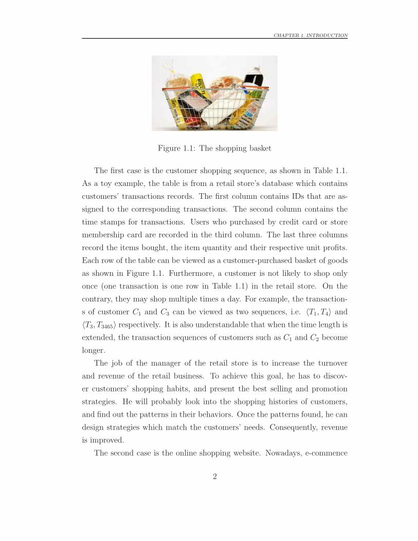
Figure 1.1: The shopping basket
The first case is the customer shopping sequence, as shown in Table 1.1.
As a toy example, the table is from a retail store’s database which contains
customers’ transactions records. The first column contains IDs that are as-
signed to the corresponding transactions. The second column contains the
time stamps for transactions. Users who purchased by credit card or store
membership card are recorded in the third column. The last three columns
record the items bought, the item quantity and their respective unit profits.
Each row of the table can be viewed as a customer-purchased basket of goods
as shown in Figure 1.1. Furthermore, a customer is not likely to shop only
once (one transaction is one row in Table 1.1) in the retail store. On the
contrary, they may shop multiple times a day. For example, the transaction-
s of customer C1 and C3 can be viewed as two sequences, i.e. 〈T1, T4〉 and
〈T3, T3465〉 respectively. It is also understandable that when the time length is
extended, the transaction sequences of customers such as C1 and C2 become
longer.
The job of the manager of the retail store is to increase the turnover
and revenue of the retail business. To achieve this goal, he has to discov-
er customers’ shopping habits, and present the best selling and promotion
strategies. He will probably look into the shopping histories of customers,
and find out the patterns in their behaviors. Once the patterns found, he can
design strategies which match the customers’ needs. Consequently, revenue
is improved.
The second case is the online shopping website. Nowadays, e-commence
2

CHAPTER 1. INTRODUCTION
Table 1.2: The Web Access Loguser id session id timestamp referring url page url action
100 1 23-10-2014 12:05:00 www.twitter.com?
user id=ABC
www.groupon.com/
view skydiving
View
100 1 23-10-2014 12:05:15 . . . www.groupon.com/
purchase skydiving
Checkout
100 1 23-10-2014 12:06:45 . . . www.groupon.com/
purchase complete
Purchase
200 1 23-10-2014 11:35:00 www.facebook.com?
user id=XYZ
www.groupon.com/
view skydiving
View
200 1 23-10-2014 11:35:30 . . . www.groupon.com/
purchase skydiving
View
200 2 23-10-2014 12:10:05 www.facebook.com?
user id=XYZ
www.groupon.com/
view yoga
View
200 2 23-10-2014 12:10:20 . . . www.groupon.com/
view boatrental
View
200 1 23-10-2014 12:10:35 . . . www.groupon.com/
view fandango
View
300 1 23-10-2014 12:01:00 www.twitter.com?
user id=ABC
www.groupon.com/
view yoga
View
300 1 23-10-2014 12:01:15 . . . www.groupon.com/
view fandango
View
300 1 23-10-2014 12:01:30 . . . www.groupon.com/
purchase fandango
Checkout
300 1 23-10-2014 12:02:30 . . . www.groupon.com/
purchase complete
Purchase
retailers such as Amazon, Groupon and Taobao are becoming very popular.
People tend to buy things online instead of going to a physical store because
of the convenience, variety, low price and many other advantages. These
websites, however, have to deal with a great number of accesses every day.
One of the backend jobs is to record the customer behaviors such as clicks
and scrolls to a web log database, as shown in Table 1.2. Each row in Table
1.2 represents an action of a user: when, where, what and how. Evidently,
a single user’s behaviors are elements of a sequence. For example, user id
= 100 probably noticed the skydiving promotion advertisements on Twitter
and happened to like to play for once. The user directly clicked the link
and purchased the bargain. All these actions are captured by Groupon’s
servers behind the web pages, and stored in their web log databases. There
3

CHAPTER 1. INTRODUCTION
are millions of such users online every day, which means the same number
of sequences in the databases are recorded. As time passes, not only do the
sequences get longer, but new sequences are also added.
Website data analysts are keen to know which items are most related
to others. With this knowledge, they can precisely recommend the items
to online users. For example, “people who buy this item also buy A, B
and C” is often seen in Amazon, and many users eventually purchase those
recommended things which they did not originally plan to buy. It is definitely
important for analysts to review and discover patterns in user behaviors to
ensure the precision of their recommendations.
0 200 400 600 800 1000 1200 1400 1600100
1010
Time (Minute #)
Buy
/Sel
l Val
ue
0
(0, 10k]
(10k, 100k]
(100k, 500k]
(500k, 1m]
(1m, 5m]
5m+
0 200 400 600 800 1000 1200 1400 1600
Figure 1.2: The stock dataset
The last case concerns the behaviors of investors in the stock trading
market, as shown in Figure 1.2. Figure 1.2 summarizes all the trader behav-
iors of a single stock from a stock exchange platform. Every small triangle
scattered in the figure represents either the sale of a certain volume of stock
(downward-pointing triangle) or the purchase of a certain volume (upward-
pointing triangle). The reference axis for the small triangles is the y-axis on
the left, which indicates the volume of stock they sell or buy, and the colors
of the triangles represent investor capital; the more capital the investor owns,
the lighter the color of the triangle. The blue line means the stock price, and
the reference y-axis is on the right. The black bars split the x-axis into differ-
ent trading days. The behaviors of the investors are clearly sequences, even
although there can be only two different actions, namely selling or buying.
4

CHAPTER 1. INTRODUCTION
To ensure the fairness of the financial market, the regulatory supervisors’
job is to uncover the tricks of manipulating the stock price of “the big play-
ers”, and take necessary actions to stop them. To acquire the knowledge,
they have to mine the trading history and determine the patterns of the
manipulators.
As can be seen from the three cases above, people in different professions
face the same problem: how to extract valuable patterns from the sequence
databases? This problem attracts a high level of attention, not only be-
cause the three examples listed above need to be solved, but also because
many other industries are involved in the sequential data analysis. To date,
researchers have proposed several methods and approaches to extract inter-
esting patterns from sequences, which are discussed in the next section.
1.2 Sequential Pattern Mining
In the 1990s, statisticians, mathematicians and computer scientists proposed
Knowledge Discovery and Data mining (KDD), which involves using a range
of models, algorithms and tools to analyze various types of data. In the a-
cademia, groups of researchers are interested in finding patterns in the trans-
actions, sequences and graphs, etc. Two branches of their research are highly
related to the topic in this thesis, thus we discuss them below.
The first branch is called frequent pattern mining, which identifies the fre-
quently repeated sub-itemsets in a transaction database as patterns. It was
first proposed in the work by Rakesh Agrawal et al. (Agrawal, Imielinski &
Swami 1993), in which the renowned downward closure property (also named
the Apriori Property) was introduced. With the foundation of the frequency-
based mining algorithms (namely, downward closure property), many follow-
up papers were subsequently published. For example, Park et al. propose
an effective hash-based algorithm for the candidate set generation (Park,
Chen & Yu 1995) . Savasere et al. present an algorithm reduces both CPU
and I/O overheads by applying partition techniques (Savasere, Omiecinski &
5

CHAPTER 1. INTRODUCTION
Navathe 1995). Several works (Agrawal & Shafer 1996, Zaki, Parthasarathy,
Ogihara & Li 1997, Cheung, Han, Ng, Fu & Fu 1996) use parallel and dis-
tributed techniques in the association rule mining. An incremental approach
is discussed in (Cheung, Han, Ng & Wong 1996), and sampling methods are
proposed in (Toivonen 1996).
The second branch is called sequential pattern mining, and has been very
popular since its introduction by Agrawal and Srikant 1995 (Agrawal &
Srikant 1995). In this work, the sequential pattern mining is defined as
follows: “Given a database of sequences, where each sequence consists of a
list of transactions ordered by transaction time and each transaction is a set
of items, sequential pattern mining is to discover all sequential patterns with
a user-specified minimum support, where the support of a pattern is the num-
ber of data sequences that contain the pattern.” For simplicity, sequential
pattern mining seeks to discover frequent subsequences as patterns in a se-
quence database (Pei, Han, Mortazavi-Asl, Pinto, Chen, Dayal & Hsu 2001).
In the first case in Section 1.1, item 45 and item 32 both appear twice in
different customers’ transactions (C1 and C5 have 45, C2 and C3 have 32),
which makes support for these items higher than for any other items’. If
the minimum support (a threshold to filter infrequent sequential patterns,
and retain frequent ones) is set to 2, then 〈45〉 and 〈32〉 are two frequent
sequential patterns.
Sequential pattern mining has proven to be essential for handling order-
based critical business problems. For retail data, sequential patterns are
useful for shelf placement and promotions, as the first case in Section 1.1.
This industry, as well as telecommunications and other businesses, may also
use sequential patterns for targeted marketing, customer retention, and many
other tasks. Other areas in which sequential patterns can be applied include
web access pattern analysis, weather prediction, production processes, and
network intrusion detection. Note that most studies of sequential pattern
mining concentrate on categorical (or symbolic) patterns,whereas numerical
curve analysis usually belongs to the scope of trend analysis and forecasting
6

CHAPTER 1. INTRODUCTION
in statistical time-series analysis (Han 2005).
In the last two decades, data mining researchers have proposed many
techniques and algorithms for mining sequential patterns. For instance, GSP
(Srikant & Agrawal 1996) uses a “Generating-Pruning” method and makes
multiple passes over the data to target the patterns; SPADE (Zaki 2001)
builds an ID-list for each candidate, and joins two k-candidates to generate
a new (k + 1)-candidate; PrefixSpan (Pei et al. 2001) extends the pattern-
growth approach in the FP-Growth algorithm(Han, Pei & Yin 2000) for fre-
quent sequential pattern mining; CloSpan (Yan, Han & Afshar 2003) propos-
es an efficient algorithm for mining closed sequential patterns; SPAM (Ayres,
Flannick, Gehrke & Yiu 2002) presents a bitmap representation of the origi-
nal sequence database, and proposes pruning methods for the I-Step/S-Step
extensions; PAID (Yang, Kitsuregawa & Wang 2006) and LAPIN (Yang,
Wang & Kitsuregawa 2007) use an item-last-position list and prefix bor-
der position set instead of the tree projection or candidate generate-and-test
techniques introduced so far; DISC-all (Chiu, Wu & Chen 2004) prunes in-
frequent sequences according to other sequences of the same length, and
employs lexicographical ordering and temporal ordering. FreeSpan (Han,
Pei, Mortazavi-Asl, Chen, Dayal & Hsu 2000) starts by creating a list of fre-
quent 1-sequences from the sequence database called the frequent item list
(f-list), and then constructs a lower triangular matrix of the items in this list.
There are two thorough surveys of the sequential pattern mining algorithms,
namely (Mabroukeh & Ezeife 2010) and (Mooney & Roddick 2013).
1.3 Actionable Knowledge Discovery
All are algorithms and techniques above have been derived by academia,
and focus on the discovery of patterns that satisfy expected technical signif-
icance, i.e. frequency. Cao et al. discovered that such approaches are not
sufficiently practical for industrial needs (Cao, Zhao, Zhang, Luo, Zhang &
Park 2010). The patterns identified by the frequent pattern (or sequential
7

CHAPTER 1. INTRODUCTION
pattern) mining methods are handed over to business people for usage in
a business environment. However, these patterns may not be informative
enough for decision-making. Surveys of data mining for business applica-
tions following the above paradigm in various domains (Cao, Yu, Zhang &
Zhang 2008) have shown that business people cannot effectively take over
and interpret the identified patterns for business use. In (Cao et al. 2010),
the issues are summarized as the three items below.
• There are often many patterns mined but they are not informative and
transparent to business people who do not know which patterns are
truly interesting and operable for their businesses.
• A large proportion of the identified patterns may be either common-
sense or of no particular interest to business needs. Business people
feel confused as to why and how they should care about the findings.
• Business people often do not know, and are also not informed, how to
interpret the findings and what straightforward actions can be taken
on them to support business decision-making and operation.
The above issues inform us that there is a large gap between academ-
ic deliverables and business expectations. Therefore, to tackle this issue,
Cao and his colleagues proposed the Domain Driven Data Mining (DDDM)
based Actionable Knowledge Discovery (AKD) (Cao & Zhang 2006, Cao
et al. 2008, Cao 2009, Cao et al. 2010, Cao 2012) to narrow down and bridge
the gap. According to (Cao et al. 2010), the AKD is a closed optimization
problem solving process from problem definition, framework/model design
to actionable pattern discovery, and is designed to deliver operable business
rules that can be seamlessly associated or integrated with business processes
and systems. Following this idea, we present the limitations and challenges
of the current sequential analysis in the next section.
8

CHAPTER 1. INTRODUCTION
1.4 Limitations and Challenges
Although sequential pattern mining algorithms successfully extract patterns
from the sequence databases, their only interestingness measurement is the
frequency of a pattern. In other words, any frequent sequential pattern is
treated as a significant one. However, in practice, most frequent sequential
patterns may not be informative for business decision-making, since they
do not show the business value and impact. In some cases, such as fraud
detection, some truly interesting sequences may be filtered because of their
low frequency. In retail business, for example, selling a car generally leads
to a much higher profit than selling a bottle of milk, while the frequency of
cars sold is much lower than that of milk. In online banking fraud detection,
the transfer of a large amount of money to an unauthorized overseas account
may appear once in over one million transactions, yet it has a substantial
business impact. Such problems cannot be tackled by the support/frequency
framework.
In a related area, the relative importance of each item is not considered
in frequent pattern mining. To address this problem, weighted association
rule mining was proposed (Cai, Fu, Cheng & Kwong 1998, Wang, Yang &
Yu 2000, Tao, Murtagh & Farid 2003, Leggett & Yun 2005, Yun 2008b, Sun
& Bai 2008, Yun & Leggett 2006b). In this framework, the weights of items,
such as unit profits of items in transaction databases, are considered. With
this concept, even if some items appear infrequently, they might still be found
if they have high weights. However, in this framework, the quantities of items
are not considered. Therefore, the requirements of users who are interested
in discovering itemsets with high sales profits cannot be satisfied, since the
profits are composed of unit profits, i.e., weights, and purchased quantities.
In view of this, utility mining emerges as an important topic in the data
mining field. Mining high utility itemsets from databases refers to finding
the itemsets with high profits. Here, the meaning of itemset utility is the
interestingness, importance, or profitability of an item to users. The utility of
items in a transaction database consists of two aspects: 1) the importance of
9

CHAPTER 1. INTRODUCTION
distinct items, which is called external utility, and 2) the importance of items
in transactions, which is called internal utility. Utility of an itemset is defined
as the product of its external utility and its internal utility. An itemset
is called a high utility itemset if its utility is no less than a user-specified
minimum utility threshold; otherwise, it is called a low-utility itemset.
Utility is introduced into frequent pattern mining to mine for patterns
of high utility by considering the quality (such as profit) of itemsets. This
has led to high utility pattern mining (Yao, Hamilton & Butz 2004), which
selects interesting patterns based on minimum utility rather than minimum
support (Liu, Liao & Choudhary 2005b, Li, Yeh & Chang 2008, Ahmed,
Tanbeer, Jeong & Lee 2009a, Wu, Fournier-Viger, Yu & Tseng 2011, Liu
& Qu 2012, Liu, Wang & Fung 2012, Wu, Shie, Tseng & Yu 2012). High
utility sequential pattern mining is substantially different and much more
challenging than high utility itemset mining. If the order between itemsets is
considered, it becomes a problem of mining high utility sequential patterns.
First, as with high utility itemset mining, the downward closure property
does not hold in utility-based sequence mining. This means that most of
the existing algorithms cannot be directly transferred, e.g. from frequent
sequential pattern mining to high utility sequential pattern mining. Second,
compared to high utility itemset mining, utility-based sequence analysis faces
the critical combinational explosion and computational complexity caused by
sequencing between sequential elements (itemsets).
1.5 Research Issues
Based on the aforementioned current research limitations, we present these
following the issues:
10
CHAPTER 1. INTRODUCTION
1.5.1 Utility-based Sequential Pattern Mining Frame-
work
The classic frequency/support-based sequential pattern mining framework of-
ten leads to many patterns being identified, most of which are not sufficiently
informative for business decision-making. For example, online banking sys-
tems may conduct the orderly processing of a great number of transactions
in one day. Another example is in the retail store, where selling a large
item such as a camera or laptop computer generally leads to much greater
profits than selling a bottle of milk. However, the meaningful pattern which
supports the selling strategy cannot be selected due to its low frequency in
the classic framework. Therefore, it is essential to incorporate utility into
sequential pattern mining to define a generic framework for high utility se-
quence mining, and to extract high value/impact/profit sequential patterns
for users.
1.5.2 Mining Top-k High Utility Sequential Patterns
Compared to classic frequent sequence mining, the utility framework provides
more informative and actionable knowledge since the utility of a sequence in-
dicates business value and impact. We are able to discover the complete set
of high utility sequential patterns with a pre-defined minimum utility thresh-
old. However, it is often difficult for users to set a proper minimum utility. A
value that is too small may produce thousands of patterns, whereas one that
is too big may result in no findings. Naturally, it would be much easier and
agreeable for users if they could select the top-k most interesting patterns.
For example, assume two databases named D1 and D2. The utilities of the
tenth highest utility sequential patterns in D1 and D2 are 35 and 8900, which
gives the minimum utility threshold of 0.02% and 1% respectively. To find
the top 10 patterns, users only need to give k = 10. Therefore, developing a
top-k high utility sequential pattern mining algorithm is essential.
11

CHAPTER 1. INTRODUCTION
1.5.3 Mining Closed High Utility Sequential Patterns
Both threshold-based and top-k-based high utility sequential pattern mining
algorithms are capable of discovering the complete set of high value patterns.
However, they usually generate a large number of patterns, thus the truly
valuable patterns in which users are interested might be flooded in hundreds
of thousands of similar patterns which have many redundancies. Another
critical issue is that the existing methods require dramatic running time and
memory when sequences are very long or the threshold is low, resulting in a
huge number of patterns being extracted. Based on the reasons above, it is
reasonable to invent a losslessly compressed representation of the high utility
sequential patterns, which is comparable to the “closed” concept in frequent
itemset/sequence mining.
1.6 Research Contributions
1.6.1 High Utility Sequential Pattern Mining
• We build the concept of sequence utility by considering the quality
and quantity associated with each item in a sequence, and define the
problem of mining high utility sequential patterns;
• A complete lexicographic quantitative sequence tree (LQS-Tree) is used
to construct utility-based sequences; two concatenation mechanisms I-
Concatenation and S-Concatenation generate newly concatenated se-
quences;
• Three pruning methods, Sequence-Weighted Utility (SWU), Sequence-
Projected Utility (SPU) and Sequence-Reduced Utility (SRU), substan-
tially reduce the search space in the LQS-Tree;
• USpan and USpan+ traverse the LQS-Tree and output all the high
utility sequential patterns.
12

CHAPTER 1. INTRODUCTION
1.6.2 Top-k High Utility Sequential Pattern Mining
• We propose a novel framework for extracting the top-k high utility
sequential patterns. A baseline algorithm TUSNaive is provided ac-
cordingly.
• Three strategies are proposed for effectively raising the thresholds at
different stages of the mining process.
• Substantial experiments on both synthetic and real datasets show that
the TUS algorithm can efficiently identify top-k high utility sequences
from large scale data with large k.
1.6.3 Closed High Utility Sequential Pattern Mining
• We propose a concise and lossless framework for discovering US-closed
high utility sequential patterns. Based on a series of novel definitions
such as maximum item utility and distinct occurrence which have n-
ever been used in state-of-art research, we theoretically prove that the
proposed representation/framework is compact and lossless.
• An efficient algorithm CloUSpan is proposed to discover US-closed high
utility sequences. We systematically analyze the extraction of US-
closed patterns on-the-fly, including the three types of newly discov-
ered patterns that can cover existing patterns, be covered by existing
patterns, or neither.
• Two effective strategies are used to enhance the performance of CloUS-
pan. Based on the framework, we proposed an early pruning strategy
and a skipping scanning strategy to avoid unnecessary searches. Both
of the strategies are not only theoretically proved, but also explained
with detailed example.
13

CHAPTER 1. INTRODUCTION
1.7 Thesis Structure
The thesis is structured as follow:
Chapter 3 incorporates utility into sequential pattern mining, and a gener-
ic framework for high utility sequence mining is defined. Two efficient algo-
rithms, namely USpan and USpan+, are presented to mine for high utility
sequential patterns. In USpan and USpan+, we introduce the lexicographic
quantitative sequence tree to extract the complete set of high utility se-
quences and design concatenation mechanisms for calculating the utility of
a node and its children with three effective pruning strategies. Substantial
experiments on both synthetic and real datasets show that USpan efficiently
identifies high utility sequences from large scale data with very low minimum
utility.
Chapter 4 proposes a novel framework called top-k high utility sequential
pattern mining to tackle this critical problem. An efficient algorithm, Top-k
high Utility Sequence (TUS) mining, is designed to identify top-k high utili-
ty sequential patterns without minimum utility. In addition, three effective
features are introduced to handle the efficiency problem, including two s-
trategies for raising the threshold and one pruning for filtering unpromising
items. Our experiments are conducted on both synthetic and real datasets.
The results show that TUS incorporating the efficiency-enhanced strategies
demonstrates impressive performance without missing any high utility se-
quential patterns.
Chapter 5 proposes a novel concise framework to discover US-closed (U-
tility Sequence closed) high utility sequential patterns, which is theoretical
proved a lossless representation of high-utility patterns. An efficient algorith-
m named CloUSpan is introduced to extract the US-closed patterns. Two
effective strategies are used to enhance the performance of CloUSpan. Both
real and synthetic datasets are used in our empirical studies. The results show
that the proposed representation is very efficient for a massive reduction in
the number of high utility sequential patterns without the loss of informa-
tion, and leads to better performance against the state-of-the-art algorithms
14

CHAPTER 1. INTRODUCTION
on all the datasets.
Chapter 6 concludes the thesis and outlines the scope for future work.
Figure 1.3 shows the research profile of this thesis.
Conclusion Future Directions
Chapter 3
Chapter 4
Chapter 5
Chapter 6
Chapter 1
Chapter 2
Utility Sequence Framework
Uspan / Uspan+ Algorithm
Background Research Issues
Related WorksContributions Foundations
Challenges
High Utility Sequential Pattern Mining SWU SPU SRU
Introduction
LiteratureReview
Algorithms
Summary
Top-KHigh Utility Sequence
Mining TUSNaive
TUSList
TUSNaive+
TUSNaive+I TUSNaive+S
TUS
MaximumItem Utility
Distinct Occurence
Vertical Utility Array
US-closure Theorem
Early Pruning SkippingScanningCloUSpan
Figure 1.3: The profile of work in this thesis
15


Chapter 2
Literature Review
In this Chapter, we first introduce the traditional frequent pattern mining
framework, which contains association rule mining, sequence mining, top-k
methods, closed patterns and weighted pattern mining. Then we introduce
the utility pattern mining framework, which contains an overview of the
research so far, high utility itemset mining, utility-based data streams, high
utility sequential pattern mining and utility-based mobile sequence mining.
2.1 Frequent Pattern Mining Framework
2.1.1 Association Rule Mining
In plain language, association rules are if/then statements that help detect
interesting relationships between items in a database. It is widely believed
that association rule mining was proposed by Rakesh Agrawal et al. (Agrawal
et al. 1993) An association rule has two parts; the “if” part is called the
antecedent and the “then” part is the consequent. Both the antecedent and
consequent are groups of items which are disjoint. In formal language, the
definition of association rule mining is as follows.
Let I = {i1, i2, . . . , in} be a set of n distinct items, also called literals.
Let D = {T1, T2, . . . , Tm} be a database of transactions where each Ti for
1 ≤ ileqm contains a set of items such that Ti ⊆ I, an association rule is
17

CHAPTER 2. LITERATURE REVIEW
an implication of the form X → Y , where X ⊆ I, Y ⊆ I are sets of items
called itemsets, and X ∩ Y = ∅. Here, X is called antecedent, and Y is
called consequent (Agrawal et al. 1993).
There are various ways to measure the interestingness of association rules.
The best-known constraints are minimum thresholds on support and confi-
dence.
• Support is the number of transactions that contain all items in the
antecedent and consequent, usually denoted as sup(X → Y ). The
relative support is defined as sup(X → Y )/|D| where |D| is the number
of transactions in D. The relative support is always in [0, 1]. Since the
size of the databases |D| greatly affects the support of the rules, the
introduction of relative support is to make it easy to compare databases
in such circumstances.
• Confidence is defined as follows.
conf(X → Y ) =sup(X ∪ Y )
sup(X)(2.1.1)
sup(X ∪ Y ) is the number of transactions that include all items in the
consequent as well as the antecedent. The range of confidence is also
in [0, 1]. This reflects how strongly X relates to Y .
The threshold values of support and confidence are usually used for filtering
strong association rules.
For example, assume I = {bread,milk, cheese, butter, cereal} and D =
{T1, T2, T3, T4}, where T1 = {bread,milk, cheese}, T2 = {cheese, butter, cereal},T3 = {milk, cheese, cereal} and T4 = {bread,milk, cereal}. The support forthe association rule cheese → milk is sup(cheese → milk) = 2 since two
transactions, namely T1 and T2, contain both milk and cheese, and the rel-
ative support is supr =sup(cheese→milk)
4= 50%. The confidence of the rule is
conf(cheese → milk) = sup({cheese,milk})cheese
= 2/3 = 66.7%. This means that
66.7% of people who bought cheese also bought milk.
18

CHAPTER 2. LITERATURE REVIEW
The Association Rule Mining Algorithms
In this section, we briefly introduce the algorithms for mining the association
rules. Generally, the association rule mining algorithms can be identified
having two phases. All frequent itemsets with a given minimum support
threshold are extracted in phase 1. Once found, the association rules can
be derived easily with a minimum confidence threshold (Agrawal & Srikant
1994). Phase 1 is far more challenging than phase 2, and has attracted
much more attention from researchers. Therefore, we focus our review on
the algorithms for mining frequent itemsets.
In 1994, Agrawal and Srikant proposed the Downward Closure Property,
also known as the Apriori Property (Agrawal & Srikant 1994).
Property 2.1 (Apriori Property) All nonempty subsets of a frequent itemset
must also be frequent; any superset of some infrequent itemset cannot be
frequent.
An itemset is said “frequent pattern” if its frequency is no less than a given
minimum support threshold. The property can be explained as follows. As-
suming X and Y are two patterns, support(X) ≤ support(Y ) if X ⊆ Y . For
example, assuming {a, b, c} is frequent, all of its sub-itemsets such as {a, c}are also frequent. If {d, e} is infrequent, its supersets such as {a, d, e} and
{d, e, f} are not frequent.
Based on the Apriori Property, Agrawal and Srikant proposed the Apriori
algorithm. The Apriori algorithm discovers the frequent patterns using a
level-wise paradigm. First, it scans the database to obtain the 1-itemset
candidates (itemsets with only one item) and prunes those infrequent ones.
Then it joins the frequent 1-itemsets to generate the 2-itemset candidates,
and retains those whose supports satisfy the minimum support and discards
those that do not. The process repeats recursively until there is no candidate
to generate, by which time the frequent itemsets have been discovered.
All of the above are candidate-generating algorithms, which means they
have to generate a huge number of candidates and check their supports by
19

CHAPTER 2. LITERATURE REVIEW
scanning the original database. Han et al. observed the shortcomings and
proposed another algorithm named FP-Growth (Han, Pei & Yin 2000).
The FP-Growth algorithm basically uses a divide-and-conquer strategy to
find frequent itemsets without using candidate generation. The foundation
of the algorithm is a Trie data structure named Frequent-Pattern tree (FP-
tree), which retains the transaction database information.
FP-Growth can be divided into two stages: pre-processing stage and min-
ing stage. In the pre-processing stage, FP-Growth scans the database D once
to obtain the frequent and infrequent 1-itemsets. The infrequent items are re-
moved from the original database, and the updated database D′ is retained.
In the mining processing stage, the FP-tree is constructed in the memory
according to D′. The FP-tree is then divided into a group of conditional
databases, each one associated with one frequent pattern. Lastly, each con-
ditional database is mined separately. The process is recursively invoked
until no conditional databases can be generated. Basically, FP-Growth re-
duces the search costs for generating candidates and scanning the original
database, thus it improves the performance to a large extent.
Eclat (Zaki 2000), is another association rule mining algorithm which
is very different from Apriori and FP-Growth. Eclat utilizes the structural
properties of frequent itemsets to facilitate fast discovery. The items are
organized into a subset lattice search space, which is decomposed into small
independent chunks or sublattices, which can be stored in memory. Efficient
lattice traversal techniques are also presented in (Zaki 2000) which quickly
identify all the long frequent itemsets and their subsets if required.
2.1.2 Frequent Sequential Pattern Mining
Frequent sequential pattern mining refers to the discovery of frequent subse-
quences as patterns in a sequence database. A sequence database consists of
sequences which are ordered list of elements, and each element can be either
an itemset or a single item. Such databases are quite common and widely
used; for example, customer shopping sequences, web clickstreams and bio-
20

CHAPTER 2. LITERATURE REVIEW
logical sequences. The formal definition of frequent sequential pattern mining
is defined below.
Let I = {i1, i2, ..., in} be a set of items. A sequence is defined as s =
〈e1, e2, ..., em〉 where ek ⊆ I, ek = ∅, 1 ≤ k ≤ m. Without loss of gen-
erality, we assume that the items in each itemset are sorted in a certain
order (such as alphabetical order). A sequence database is defined as D =
{[sid1, s1], [sid2, s2], ..., [sidl, sl]}. The sid is the unique identification of the
corresponding sequence. A sequence α = 〈a1, a2, ..., ap〉 is called a sub-
sequence of another sequence β = 〈b1, b2, ..., bq〉, denoted by α ⊆ β, if
and only if ∃j1, j2, ..., jp, such that 1 ≤ j1 < j2 < ... < jp ≤ n and
a1 ⊆ bj1 , a2 ⊆ bj2 , ..., ap ⊆ bjp. We also call β the supersequence of α, or
β contains α. Given a sequence database D, the support of α is the number
of sequences in D which contain α. If the support α satisfies a minimum
support threshold, α is a frequent sequential pattern.
For example, we assume the itemset I sold in some retail stores is as
follows.
I = {bread,milk, cheese, butter, cereal, oatmeal}
Table 2.1: Sequence Database
sid tid transactions
1 1 bread, butter, cereal
1 2 milk, cheese, oatmeal
1 3 bread, butter
2 1 cheese, butter
2 2 bread,milk, cheese, oatmeal
2 3 milk
3 1 bread, cheese, butter
3 2 bread,milk, oatmeal
A toy sequence database D with I would be as shown in Table 2.1. The
database consists of three sequences, which represent the shopping histories
21
CHAPTER 2. LITERATURE REVIEW
of three customers. Both sequence sid = 1 and sid = 2 contain 3 itemsets
(transactions), and sid = 3 contains 3 itemsets. Equally, D in Table 2.1 can
be written as:
s1 = 〈(bread, butter, cereal)(milk, cheese, oatmeal)(bread, butter)〉s2 = 〈(cheese, butter)(bread,milk, cheese, oatmeal)milk〉s3 = 〈(bread, cheese, butter)(bread,milk, oatmeal)〉
Speaking of the containment relationship, 〈butter(bread,milk)〉 can be
a subsequence of s2 and s3 but not s1. Similarly, 〈buttercheese〉 can be a
subsequence of s1 and s2 but not s3.
Quite a few algorithms have been proposed since it was first introduced
in (Agrawal & Srikant 1995). For instance, GSP (Srikant & Agrawal 1996)
uses a “Generating-Pruning” method and makes multiple passes over the
data to target the patterns; SPADE (Zaki 2001) builds an ID-list for each
candidate, and joins two k-candidates to generate a new (k + 1)-candidate;
PrefixSpan (Pei et al. 2001) extends the pattern-growth approach in FP-
Growth algorithm (Han, Pei & Yin 2000) for frequent sequential pattern
mining; CloSpan (Yan et al. 2003) proposes an efficient algorithm for min-
ing closed sequential patterns; SPAM (Ayres et al. 2002) presents a bitmap
representation of the original sequence database, and proposes pruning meth-
ods for the I-Step/S-Step extensions; PAID (Yang et al. 2006) and LAPIN
(Yang et al. 2007) use an item-last-position list and prefix border position
set instead of the tree projection or candidate generate-and-test techniques
introduced so far; DISC-all(Chiu et al. 2004) prunes infrequent sequences ac-
cording to other sequences of the same length, and employs lexicographical
ordering and temporal ordering. FreeSpan (Han, Pei, Mortazavi-Asl, Chen,
Dayal & Hsu 2000) starts by creating a list of frequent 1-sequences from the
sequence database called the frequent item list (f-list), and then constructs
a lower triangular matrix of the items in this list.
All of the above algorithms rely on the downward closure property. Next,
22

CHAPTER 2. LITERATURE REVIEW
we briefly introduce the algorithms above.
AprioriAll
AprioriAll (Agrawal & Srikant 1995) is believed to be the first algorithm
solve sequential pattern mining. First, it finds all frequent 1-patterns whose
support values satisfy a user-defined minimum support. Then, it initializes
and maintains two types of list containers, namely the candidate lists and the
frequent pattern lists. For every (k + 1)-candidate constructed by joining two
frequent k-patterns (the patterns with k items in the frequent pattern list),
the support needs to be scanned from the original database. The process
repeats until no further patterns can be found.
GSP
GSP (Generalized Sequential Patterns) (Srikant & Agrawal 1996) is a sequen-
tial pattern mining method that was developed by Srikant and Agrawal in
1996 and has been very popular since then. It is an extension of the Apriori
algorithm (Agrawal & Srikant 1995) for sequence mining. The main struc-
ture is similar to AprioriAll (Agrawal & Srikant 1995), and the details are as
follows. First, it scans the database to obtain the frequent 1-sequences. Then
it generates the next level candidates by joining the previous level frequent
sequences, the same as AprioriAll. The differences are in the candidate gen-
eration and candidate support counting. In the candidate generation stage,
they use a mechanism to prune the unpromising candidates. Thus in the
same level (candidates of the same length), the number of candidates is no
more than that of AprioriAll. In the support counting stage, a hash-tree
data structure is used to reduce the number of candidates to be checked.
The representation of the database is transformed to efficiently determine
whether a specific candidate is contained in the database.
23
CHAPTER 2. LITERATURE REVIEW
SPADE
SPADE (Sequential PAttern Discovery using Equivalent classes) (Zaki 2001)
is also a level-wise sequential pattern mining algorithm that uses a vertical
data format. The key difference between SPADE and AprioriAll (Agrawal
& Srikant 1995) and GSP (Srikant & Agrawal 1996) is that SPADE avoids
scanning the original database or a representation. Instead, SPADE builds
an ID-list(a list of the IDs of sequences and elements) for each candidate. The
support count of the candidate can be easily calculated from its ID-list, which
greatly reduces the cost of scanning. Because of this, SPADE outperforms
GSP to a large extent according to authors’ experimental results.
FreeSpan
FreeSpan (Frequent pattern-projected Sequential pattern mining) (Han, Pei,
Mortazavi-Asl, Chen, Dayal & Hsu 2000) is the first projection-based depth-
first algorithm proposed by Han et al. in 2000. Similar to the previous algo-
rithms, FreeSpan scans the database once to obtain the frequent 1-sequences
and put them in the f-list(frequent item list). Then it constructs a matrix
called S-Matrix which contains the 2-sequences and their supports generated
from the f-list, and the infrequent ones are filtered. Each sequential pattern
in the S-Matrix corresponds to a projected database that all the sequences
contain the sequential pattern itself. The next step is to construct level-2-
sequences from the S-Matrix and find annotations for repeating items and
projected databases in order to discard the matrix and generate level-3 pro-
jected databases. The process repeats until no candidates can be generated.
SPAM
SPAM (Sequential PAttern Mining) (Ayres et al. 2002) is a depth-first al-
gorithm that integrates the ideas of GSP (Srikant & Agrawal 1996), S-
PADE (Zaki 2001) and FreeSpan (Han, Pei, Mortazavi-Asl, Chen, Dayal
& Hsu 2000). A group of novel concepts such as the sequence-extension
24

CHAPTER 2. LITERATURE REVIEW
step (S-Step), itemset-extension step (I-Step) and the lexicographical tree
are firstly introduced. Similar to FreeSpan, SPAM uses a depth-first strate-
gy to traverse the lexicographical tree to extract the complete set of frequent
sequential patterns. More importantly, SPAM encodes the ID-list from S-
PADE to a vertical bitmap data structure and puts them in the memory so
that the “joining” operation between two ID-lists is extremely fast. That is
the key reason why SPAM outperforms any of the previous algorithms.
In Chapter 3, we extend the lexicographic tree to complete-LQS-Tree to
address the high utility sequential pattern mining.
PrefixSpan
PrefixSpan (Prefix-projected Sequential pattern mining) (Pei et al. 2001) is
an algorithm that extends the pattern-growth approach for frequent pat-
tern mining and the first algorithm that does not generate a candidate. As
an enhanced algorithm of FreeSpan (Han, Pei, Mortazavi-Asl, Chen, Dayal
& Hsu 2000), PrefixSpan uses the “prefix” of the sequence to project the
database. Then it scans the projected database for the items to be concate-
nated to the prefix, and counts the support for each item. The infrequent
concatenation items will be discarded, and frequent items will be retained.
Lastly, for each frequent concatenation item, a new prefix and its correspond-
ing smaller projected database can be constructed. The process continues
until no more frequent concatenation items can be scanned. In experimental
results, PrefixSpan performs much better than both GSP and FreeSpan. The
major cost of PrefixSpan is the construction of projected databases.
In Chapter 3, we follow main structure of PrefixSpan to design the USpan
algorithm.
PAID and LAPIN
PAID (PAssed Item Deduced sequential pattern mining) (Yang et al. 2006)
and LAPIN (LAst Position INduction sequential pattern mining) (Yang et al.
2007) essentially follow pattern-growth algorithms such as FreeSpan (Han,
25
CHAPTER 2. LITERATURE REVIEW
Pei, Mortazavi-Asl, Chen, Dayal & Hsu 2000) and PrefixSpan (Pei et al.
2001). The main contribution of PAID is that it adopts a novel strategy
to reduce the scanning cost. The technical detail is as follows. In a prefix-
sequence projection, the last position (the itemset number) of an item can
be used to judge whether or not the item can be extended to the current
prefix. For instance, s0 = 〈(ab)〉 is contained in s1 = 〈(ab)a(cd)ea〉, s2 =
〈(ab)(ae)〉 and s3 = 〈(abc)aea〉. Since the last position of a in s1 is 5 (the
fifth itemset contains a, similarly 2 in s2 and s3), there is no need to scan the
sequences to obtain a. Instead, PAID only needs to compare the projection
positions with the last positions of a in the three sequences. That is a simple
example to explain the basic idea of PAID, and more complex designs in the
implementation of algorithm.
DISC-all
DISC-all (DIrect Sequence Comparison) algorithm (Chiu et al. 2004) was
proposed by Chiu et al. in 2004. The key element of DISC-all algorithm
is the DISC strategy. It discovers the frequent k-sequences without having
to compute the support counts of the non-frequent sequences. In detail, the
authors define the order of two sequences having the same length. Given two
sequences, they examine the items of both from left to right and compare the
leftmost distinct items by alphabetical order. For example, 〈abh〉 is smaller
than 〈acf〉 because b, in the second place, is smaller than c. The DISC
strategy then finds the minimum subsequences of each sequence, and sorts
the sequences according to the ascending order of these subsequences with the
same length. Therefore, the DISC-all algorithm can skip many non-frequent
candidate subsequences and save costs. The updating process in the DISC-
all algorithm involves searching the (k-1)-prefix projected database, which is
similar to the mining process of PrefixSpan (Pei et al. 2001).
26

CHAPTER 2. LITERATURE REVIEW
2.1.3 Top-K Frequent Itemset/Sequence Mining
Sometimes it is difficult for users to provide suitable minimum support for
frequent itemsets/sequential patterns mining, because to determine an appro-
priate minimum support threshold, detailed knowledge about the database
is necessary. There is a range of factors such as the distribution of the item-
s, density of the database and length of transactions which could affect the
number of patterns generated by a specific threshold. A threshold that is too
small may lead to the generation of thousands of itemsets, whereas a thresh-
old that is too big may generate no answers. However, if users can simply
select the highest support patterns with a given number, that is, the top-k
frequent patterns, the problem is solved. Mining top-k patterns is a challeng-
ing area. LOOPBACK and BOMO (Cheung & Fu 2004) were proposed for
mining the N k-itemsets with the highest supports for k up to a certain kmax
value. The ExMiner (Quang, Oyanagi & Yamazaki 2006) algorithm pro-
posed a two-phase mining, including the “explorative mining” and “actual
mining” phases to select top-k frequent itemsets. Wang, et al. (Wang, Han,
Lu & Tzvetkov 2005) and Han, et al. (Han, Wang, Lu & Tzvetkov 2002)
proposed a top-k closed pattern/itemset mining method TFP without mini-
mum support. The TFP starts the mining at minimum support = 0, and it
rises quickly by using the length constraint and the properties of the top-k
frequent closed itemsets. Some pruning methods on FP-Tree are used to re-
duce the search space as well. While TFP focuses on mining frequent closed
itemsets, Tzvetkov, et al. (Tzvetkov, Yan & Han 2005) studied top-k closed
sequential pattern mining and proposed the TSP algorithm, which uses simi-
lar approaches as (Wang et al. 2005) and (Han et al. 2002) by extending them
from frequent itemset mining. Although the algorithms can efficiently dis-
cover top-k frequent sequences, it is difficult to adapt the ideas to the utility
framework since the downward closure property does not hold. Chuang et al.
proposed MTK and MTK Close algorithms(Chuang, Huang & Chen 2008),
and first attempted to specify the available upper memory size that can be
utilized by mining frequent itemsets.
27

CHAPTER 2. LITERATURE REVIEW
2.1.4 Closed Frequent Itemset/Sequence Mining
A major challenge in mining frequent patterns from a large dataset is the fact
that a large number of patterns is usually generated, and many of them are
redundant. This happens especially when the minimum support threshold
is low. This is because if a pattern is frequent, all of its subpatterns are
frequent as well. A very long pattern will contain an exponential number
of smaller, frequent sub-patterns, which makes the number of patterns grow
explosively. On the other hand, truly valuable patterns in which users might
be interested might be flooded in hundreds of thousands of similar patterns.
Closed Frequent Itemset Mining
A pattern is said to be closed if there is no super-pattern that has the same
support. For example, if {a, b, c} is a closed pattern, the support of any of its
super-patterns must be less than that of {a, b, c}. Given a database D and a
threshold ξ, the closed itemset/sequence mining means finding all the closed
patterns (say LC represents the pattern set) in D which satisfy ξ. Assume
that Lmeans all the frequent patterns whose supports are no less than ξ. It is
evident that L can be completely recovered from LC. In other words, closed
frequent patterns provide a compact and lossless representation of frequent
patterns.
The mining of frequent closed itemsets was first introduced by Pasquier et
al. in 1999 (Pasquier, Bastide, Taouil & Lakhal 1999). They define the closed
itemset lattice by using a closure mechanism based on the Galois connection
and Galois lattice theory (Birkhoff 1967, Davey & Priestley 1994). They also
propose an Apriori-based algorithm called A-Close (Pasquier et al. 1999)
to mine the closed frequent patterns. Pei et al. developed the CLOSET
algorithm (Pei, Han &Mao 2000) based on the FP-tree (Han, Pei & Yin 2000)
data structure for mining closed itemsets without candidate generation, and
they developed a single prefix path compression technique to quickly identify
frequent closed itemsets.
Zaki and Hsiao proposed CHARM algorithm (Zaki & Hsiao 2002, Zaki
28

CHAPTER 2. LITERATURE REVIEW
& Hsiao 2005) in 2002. CHARM simultaneously explores both the itemset
space and transaction space, which is different from previous association
mining methods which only exploit the itemset search space. CHARM also
avoids enumerating all possible subsets of a closed itemset when enumerating
the closed frequent sets.
Calders and Goethals proposed the NDI algorithm to mine a new repre-
sentation called non-derivable frequent itemsets in 2002 (Calders & Goethals
2002). They present deduction rules to derive tight bounds on the support
of candidate itemsets, and they illustrate how the deduction rules allow for
constructing a minimal representation for all frequent itemsets.
Wang et al. proposed the CLOSET+ algorithm (Wang, Han & Pei 2003)
as an extension work on CLOSET (Pei et al. 2000) in 2003. CLOSET+
is a depth-first search and horizontal format-based method which computes
the local frequent items of a prefix by building and scanning its projected
database. A number of strategies are proposed to prune the search space.
The FPclose algorithm (Grahne & Zhu 2003) is another work based on
FP-tree and FP-Growth and was proposed by Grahne and Zhu in 2003. The
main contribution of the paper is a novel technique that uses an array to
greatly improve the performance of the algorithms operating on FP-trees.
Based on this, the authors proposed FPmax∗ to mine the maximal frequent
patterns and FPclose for the closed patterns.
Lucchese et al. proposed DCI CLOSED (Lucchese, Orlando & Perego
2006) in 2006. Basically, DCI CLOSED works with three sets, namely CLO-
SED SET, PRE SET and POST SET. The CLOSED SET contains the closed
frequent itemsets found so far, and the other two are temporary container-
s which work together in the procedure to generate the final results. The
authors analyzed the density of the datasets affects the performance of the
algorithm. Correspondingly, DCI CLOSEDd is proposed for dense datasets
and DCI CLOSEDs is for sparse datasets.
MT CLOSED (Lucchese, Orlando & Perego 2007) is a parallel closed
itemset mining algorithm also proposed by Lucchese et al., who designed and
29

CHAPTER 2. LITERATURE REVIEW
tested several parallelization paradigms by investigating the static/dynamic
decomposition and scheduling of tasks, thus showing the scalability with re-
gard to the number of CPUs. They analyzed the performance of MT CLOSED
in terms of harnessing CPUS and cache friendliness. They provided addition-
al speed-up by introducing SIMD extensions.
Closed Frequent Sequence Mining
Closed frequent sequential pattern mining is slightly different from closed
frequent itemset mining. The definition is as follows. Given a database Dand a minimum support ξ, assume L contains all the frequent sequential
patterns in D that satisfy ξ. The closed frequent sequential pattern set C is
defined as C = {α|α ∈ L ∩ �β ∈ L such that α ⊆ β ∩ sup(α) = sup(β)}. Aswith closed frequent itemset mining, the relation between L and C is that
C ⊆ L.CloSpan (Yan et al. 2003) proposed by Yan et. al. is the first algorithm
to mine the closed frequent sequential patterns. In their paper, the auhtors
re-explored the Lexicographic Sequence Tree which first appeared in (Ayres
et al. 2002), and proposed strategies to modify the links in the tree such
that the correct C can be guaranteed. Based on that, they proposed the
backward sub-pattern and backward super-pattern to avoid certain invalid
searches. Experimental results show that CloSpan outperforms PrefixSpan
to a large extent.
BIDE (Wang & Han 2004) was proposed by Wang and Han in 2004. The
key contribution is a new paradigm called bi-directional (forward and back-
ward) extension for mining closed sequences without candidate maintenance.
The forward directional extension is for growing the prefix patterns and also
for checking the closure of prefix patterns, while the backward directional
extension can be used both to check the closure of a prefix pattern and to
prune the search space. Two pruning methods, BackScan and ScanSkip,
were proposed to optimize performance. One thing we need to mention here
is that, BIDE can only mine the one-item-element sequences. For example,
30

CHAPTER 2. LITERATURE REVIEW
〈cadbabd〉 is fine since the elements in the sequence are only 1-item. How-
ever, sequences like 〈c(ad)b(abd)〉 which are acceptable with CloSpan cannot
be processed by BIDE. Therefore, any dataset that BIDE can process is a
subset of CloSpan and Prefixspan.
Par-CSP (Cong, Han & Padua 2005) is a parallel closed frequent sequence
mining algorithm proposed by Cong et al. It is a serial algorithm extended
from BIDE. To efficiently parallelize BIDE, Par-CSP uses the divide-and-
conquer strategy to minimize inter-processor communications. A method
called dynamic scheduling is used to reduce processor idle time, and the
authors devise a technique called selective sampling to estimate the relative
mining time of the subtasks and achieve load balancing.
TSP (Tzvetkov et al. 2005) is a projection-based top-k mining algorithm
proposed by Tzvetkov et al. Besides the closure constraint, TSP also adds
a minimum length constraint on the resultant patterns. This means that a
sequential pattern whose length (the number of items in a sequence) is less
than the predefined minimum length will be discarded in all conditions. The
key part of TSP is a multi-pass search space traversal strategy. Since TSP
is a top-k mining algorithm, the minimum support threshold is pre-defined.
The strategy proposed by Tzvetkov et al. is to ensure that patterns found
so far are closed, and at same time to raise the minimum support as quickly
as possible.
COBRA (Tzvetkov et al. 2005) was proposed by Huang et al. in 2005.
Although algorithms such as CloSpan and BIDE had already been proposed
for mining closed sequential patterns by the time COBRA was proposed, the
authors argued that these projection-based methods suffered from duplicate
item extension and expensive matching cost. To tackle these issues, COBRA
first conducts item extension and then carries out sequence extension. The
efficiency comes from the removal of database scans and the compressed
strategy of the bi-phase reduction approach.
31

CHAPTER 2. LITERATURE REVIEW
2.1.5 Weighted Frequent Itemset/Sequence Mining
Weighted frequent itemset/sequence mining is more practical than frequen-
t pattern mining because it considers the different semantic significance
(weight) of the items, which is not considered in the frequency/support frame-
work. The definition of weighted frequent pattern mining is as follows.
Let I = {i1, i2, ..., in} be a set of items and D = {T1, T2, ..., Tm} be a
database of transactions where Tk ⊆ I(1 ≤ k ≤ m). Every item in I is
associated with a weight, denoted as w(ik)(1 ≤ k ≤ n). The weight and
weighted support of l-itemset (itemset with l items) P l are denoted and
defined as
weight(P l) =
∑i∈P l w(i)
l(2.1.2)
wsup(P l) = weighted(P l)× sup(P l) (2.1.3)
P l is called a weighted frequent pattern if wsup(P l) is no less than a pre-
defined threshold. Weighted frequent sequence mining has similar definitions.
Early works such as MINWAL (Cai et al. 1998), WAR (Wang et al. 2000)
and WARM (Tao et al. 2003) exploit a level-wise approach to generate-and-
test the candidates. The disadvantages of these algorithms is that mul-
tiple database scans are required, thus performance turns out to be very
poor. In 2005, Yun & Leggete proposed the WFIM algorithm (Leggett
& Yun 2005) which extends from FP-Tree structure. WLPMiner (Yun &
Leggett 2005, Yun 2008a) discovers weighted frequent patterns using length
decreasing support constraints. WIP (Yun & Leggett 2006b, Yun 2007a)
mines weighted interesting patterns with a strong weight and/or support
affinity. WCloset (Yun 2007b) extracts lossless closed weighted frequent pat-
terns. WSpan (Yun & Leggett 2006a, Yun 2008b) detects weighted frequent
sequential patterns. Ahmed et al. proposed SPWIP-tree structure (Ahmed,
Tanbeer, Jeong & Lee 2008) which uses a single-pass of database to capture
the weighted interesting patterns. (Chang 2011) presents a new framework
for finding time-interval weighted sequential (TiWS) patterns in a sequence
32

CHAPTER 2. LITERATURE REVIEW
database and time-interval weighted support (TiW-support) to find the Ti-
WS patterns. MWSA (Lee & Yun 2012) mines weighted frequent sub-graphs
with weight and support affinities. MWFIM (Yun, Shin, Ryu & Yoon 2012)
is for mining maximal weighted frequent patterns. IWFPWA and IWFPFD
(Ahmed, Tanbeer, Jeong, Lee & Choi 2012) are two algorithms for incremen-
tal and interactive WFP mining.
2.2 Utility Framework
So far, we have reviewed a range of pattern mining algorithms which aim
to discover various types of patterns such as itemsets, sequences and graph-
s. These algorithms, however, only select high frequency/support patterns.
Patterns below the minimum threshold are considered useless and are dis-
carded. Frequency is the only interestingness measurement, and all item-
s and transactions are treated equally in such a framework. Clearly, this
assumption contradicts the truth of many real world applications, because
the importance of different items/itemsets/sequences might be significantly
different. In these circumstances, the frequency/support framework is in-
adequate for pattern selection. Based on the above concerns, researchers
proposed the utility-based data mining defined as below:
Definition 2.1 Let D be a database that consists of a set of homogenous
records {r1, r2, ..., rn}, where each record rj(1 ≤ j ≤ n) is defined as
rj = f(ir1, ir2 , ..., irq) (2.2.1)
irk(1 ≤ k ≤ q) is selected from I = {i1, i2, ..., im}, a list of universal distinct
atom items. This means that the items in rj are organized by the f function.
The utility-based record is defined as
ruj = f((ir1 , u1), (ir2 , u2), ..., (irq , uq)) (2.2.2)
uk(1 ≤ k ≤ q) is the utility value of the item. This means that each item
in rj is associated with a utility, and Du means that the records in D are
utility-based records.
33

CHAPTER 2. LITERATURE REVIEW
The main difference between the frequency/support framework and the
utility framework is that the items in the latter are associated with a u-
tility while the former they are not. The reason for this is to break the
equal importance between two objects. This might be abstract and difficult
to understand. In the following subsections, we will provide more specific
definitions in terms of different types of high utility data mining.
2.2.1 The Overview of High Utility Data Mining
Before reviewing the papers in high utility data mining, we present an overview
picture of the major algorithms and the connections in this area, as shown in
Figure 2.1. The x-axis represents the year, and the y-axis is composed of dif-
ferent research tracks, namely different sub-directions and sub-sub-directions.
Each item in either a bubble or a rectangular plotted in the coordinate rep-
resents an algorithm which solves a certain utility mining problem. Three
types of edges of the items are used: 1) the dashed line edge bubble means
the algorithm is only published in a conference of that year; 2) the solid
line means the paper is published in a journal; 3) the solid rectangular indi-
cates that the algorithm was first published in a conference of that year, and
that a journal paper was published later. We classified all the high utility
mining algorithms to two main tracks, namely high utility itemset mining
and high utility sequence mining. The high utility itemset mining consists
of: 1) mining high utility patterns, 2) incremental high utility itemset min-
ing, and 3) mining high utility itemsets in data streams. The high utility
sequence mining is composed of high utility sequential pattern mining and
high utility mobile sequence mining. In fact, the topics in the tracks are var-
ied. For example, UWPTPM and IUWAS-tree discuss web mining, UP-Span
concerns episode mining, and US/UI presents high utility sequential pattern
mining. To simplify the diagram, we merge them into one track. For the
links between items, the dashed line means that the previous paper’s first
author is different from the work that follows, otherwise a solid line is used.
Two linked items indicate that the later item compares the previous one in
34

CHAPTER 2. LITERATURE REVIEW
their experiments. In the following sections, we will discuss these algorithms
in detail from the high utility itemset mining track to the sequence mining
track.
35

CHAPTER
2.LIT
ERATURE
REVIE
W
Hig
h U
tility
Item
set M
inin
g
UP-Growth
US/UI
TKU
USpan
HUI-Miner
d2HUP
TUS
IHUP
CloUSpan
UP-Span
CHUDIIDS
Foundation
Two-Phase
IUWAS-tree
Pre-HUI
PHUS
CHUI-Mine
OOApriori
CTU-PROL
MHUI-TIDTHUI-Mine
GUIDE
HUQA
FUP-HUI
UMSP UM-Span IM-Span
Mining High Utility Patterns
Incremental High Utility Itemset Mining
Mining High Utility Itemsets in Data Streams
High Utility Mobile Sequence Mining
High Utility SequentialPattern Mining
Hig
h U
tility
Seq
uenc
e M
inin
g
Same group
Different groups
Journal
Conference
HUC-PruneCTU-Mine
HUPMS
PFUS
2003 2004 2005 2006 2007 2009 2010 2011 2012 2013 20142008
CTU-PRO
Conference& Journal
Udepth
FHM
Figure 2.1: The high utility mining algorithms
36
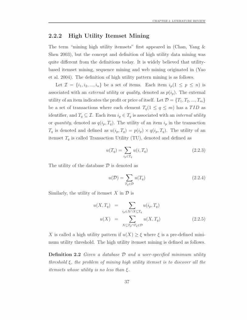
CHAPTER 2. LITERATURE REVIEW
2.2.2 High Utility Itemset Mining
The term “mining high utility itemsets” first appeared in (Chan, Yang &
Shen 2003), but the concept and definition of high utility data mining was
quite different from the definitions today. It is widely believed that utility-
based itemset mining, sequence mining and web mining originated in (Yao
et al. 2004). The definition of high utility pattern mining is as follows.
Let I = {i1, i2, ..., in} be a set of items. Each item ip(1 ≤ p ≤ n) is
associated with an external utility or quality, denoted as p(ip). The external
utility of an item indicates the profit or price of itself. LetD = {T1, T2, ..., Tm}be a set of transactions where each element Tq(1 ≤ q ≤ m) has a TID as
identifier, and Tq ⊆ I. Each item ip ∈ Tq is associated with an internal utility
or quantity, denoted as q(ip, Tq). The utility of an item ip in the transaction
Tq is denoted and defined as u(ip, Tq) = p(ip) × q(ip, Tq). The utility of an
itemset Tq is called Transaction Utility (TU), denoted and defined as
u(Tq) =∑
ip∈Tq
u(i, Tq) (2.2.3)
The utility of the database D is denoted as
u(D) =∑
Tq∈Du(Tq) (2.2.4)
Similarly, the utility of itemset X in D is
u(X, Tq) =∑
ip∈X∩X⊆Tq
u(ip, Tq)
u(X) =∑
X⊆Tq∩Tq∈Du(X, Tq) (2.2.5)
X is called a high utility pattern if u(X) ≥ ξ where ξ is a pre-defined mini-
mum utility threshold. The high utility itemset mining is defined as follows.
Definition 2.2 Given a database D and a user-specified minimum utility
threshold ξ, the problem of mining high utility itemset is to discover all the
itemsets whose utility is no less than ξ.
37

CHAPTER 2. LITERATURE REVIEW
Table 2.2: Quality Table
item a b c d e f
weight/quality 3 5 4 2 1 1
Table 2.3: Transaction TableTID Transactions TU
T1 (a,2)(d,4)(e,1) 15
T2 (e,2)(f,2) 4
T3 (a,1)(b,1)(c,4)(d,5) 34
T4 (b,2)(d,5)(e,3) 23
T5 (a,1)(c,2)(d,5)(e,3) 24
We explain the definitions above by illustrating the example database
shown in Table 2.2 and Table 2.3. Table 2.2 is the quality table which contains
the external utilities of all the items, namely I = {a, b, c, d, e, f}. Table 2.3
is the transaction table where the items in each transaction are associated
with an internal utility. For example, (a, 2) in T1 means the quantity of a
is 2. Therefore, the utility of (a, 2) in T1 is u(a, T1) = 3 × 2 = 6, which
indicates the profit/price of a is 6. Furthermore, the utility of T1 is u(T1) =
u(a, T1)+u(d, T1)+u(e, T1) = 6+8+1 = 15. It is also called the transaction
utility of T2. The utility of the whole database is u(D) = u(T1) + u(T2) +
... + u(T5) = 15 + 4 + ... + 24 = 100. The utility of itemset {ad} in T1
is u({ad}, T1) = 6 + 8 = 14, and the utility in the database is u({ad}) =
14+13+13 = 40. Assume ξ = 35, then {ad} is a high utility itemset. Other
high utility itemsets are {acd}, {bd}, {cd}, {d} and {de} with the utilities of
50, 35, 44, 38 and 35 respectively.
We explain why the downward closure property does not hold in high
utility pattern mining. The property states that a pattern’s support is no
less than that of its super-pattern. However, when it comes to the utility
framework as in the examples above, the utility of {d} is 38, which is bigger
than 35 (the utility of {de}) and smaller than 50 (the utility of {acd}). Both
38

CHAPTER 2. LITERATURE REVIEW
{acd} and {de} are the super-patterns of {d}, but the utilities could be either
bigger or smaller. It obviously does not hold the downward closure property
any more.
Next, we introduce the high utility itemset mining algorithms.
Foundational Approach
In 2004, Yao et al. published the paper “A Foundational Approach to Mining
Itemset Utilities from Databases” (Yao et al. 2004) in Siam Data Mining (S-
DM) conference. It is widely believed that this was the first and foundational
paper of high utility pattern mining. The authors first defined the problem
of mining high utility itemsets, and a theoretical model of utility mining was
proposed. Specifically, two types of utilities for items, namely transaction
utility (referred as internal utility in our definitions above) and external u-
tility, were first proposed. The utility calculation functions are exactly the
same as the definitions above and are explained in the examples.
Although high utility pattern mining is essential to many applications,
to mine the new patterns is quite challenging, because the new problem no
longer holds the downward closure property. In other words, a pattern’s
utility might be larger, equal to or smaller than its super- or sub-pattern.
This is very different from traditional frequent pattern mining.
To tackle this problem, the authors present a utility upper bound called
Expected Utility for the itemset. The definition is as follows:
u′(Ik) =supmin(Ik)
k − 1
k∑
i=1
u(Ik−1i )
sup(Ik−1i )
(2.2.6)
where,
supmin(Ik) = min∀Ik−1
ip⊂Ik
{sup(Ik−1ip
)} (2.2.7)
The notations in the equations are as follows. u′ is the proposed expected
utility of Ik, an itemset with k items. In plain words, the supmin of Ik is the
support of the least frequent sub-(k-1)-itemset of itself. Since the number of
39

CHAPTER 2. LITERATURE REVIEW
Ik’s sub-(k-1)-itemsets (denoted as Ik−1) is k, and the calculation of u′(Ik)
requires all of Ik−1s’ supports and utilities, the function is not very efficient.
Thus, the authors further proposed an upper bound on u′(Ik), which can be
used to prune unpromising candidates.
Two-Phase Algorithm
The Two-Phase Algorithm (Liu, Liao & Choudhary 2005a, Liu et al. 2005b)
was proposed by Liu et al. in 2005, and is one of the most cited papers
in utility-based data mining. Just as its name suggests, the Two-Phase
algorithm has two phases. In the first phase, it generates a set of high utility
candidates, and all the high utility itemsets are in this set. In the second
phase, an extra database scan is performed to filter the high utility itemsets
from the candidates. The key contribution of Two-Phase is the proposal of
the Transaction-Weighted Downward Closure Property.
The Transaction-weighted Downward Closure Property (TDCP) is quite
similar to the Apriori Property (or the Downward Closure Property) in tra-
ditional frequent pattern mining. It states that
TWU(Ik) ≤ TWU(Ik−1) (2.2.8)
whereas the Apriori Property states that
sup(Ik) ≤ sup(Ik−1) (2.2.9)
The critical element is the calculation of TWU . In (Liu et al. 2005b),
the TWU is short for Transaction-Weighted Utilization and is defined as the
sum of the transactions’ utilities which contain the itemset. The equation of
TWU is
TWU(Ik) =∑
Ik⊆Tq∩Tq∈Du(Tq) (2.2.10)
It is not very difficult to understand u(Ik) ≤ TWU(Ik), because for
every Tq ∈ D, if Ik ⊆ Tq, then u(Ik) ≤ u(Tq) = TWU(Ik). Therefore,
40

CHAPTER 2. LITERATURE REVIEW
suppose HTWU to be the set of itemsets whose TWU is no less than the
minimum utility threshold ξ, and HU to be the high utility itemsets. Then
HU ⊆ HTWU . The Two-Phase algorithm extracts the HTWU in the first
phase with the help of TDCP, then it scans for HU in the second phase.
Compared with (Yao et al. 2004), Two-Phase generates fewer candidates
and is much less costly. From the Two-Phase calculation functions, the TWU
of Ik is independent to that of Ik−1, and the upper bound TWU is tighter
than the Expected Utility. The theoretical conclusions are further proved
in the authors’ experimental results. Because of the simplicity, clean nature
and low complexity, Two-Phase was the benchmark algorithm of many other
high utility mining algorithms, and TWU has had an influential impact on
the follow-up design of the upper bound of utility mining problems.
In Chapter 3, we extend the TWU to the Sequence-Weighted Utilization,
namely SWU , and we further proposed the SDCP , i.e. Sequence-weighted
Downward Closure Property on the basis of TWDC in (Liu et al. 2005b).
Isolated Items Discarding Strategy
The Isolated Items Discarding Strategy (IIDS) (Li, Yeh & Chang 2008) was
proposed by Li et al. in 2008. The IIDS is similar to Transaction-Weighted
Utilization (TWU) but has a tighter upper bound. Instead of scanning the
database once to obtain the items’ TWU and discard low TWU items, the
IIDS strategy recursively scans the database many times. In each scan,
unpromising items are removed from the database, and the smaller updated
database is the input for the next scan. The detailed procedure is shown
as Algorithm 2.1. The input D0 is the original database, and the output
D∗ represents the minimized database. In the algorithm, line 1 - 2 are the
preparation for the later multiple scanning, and line 3 - 5 constitute the
while loop for reducing the size of D∗. Every time D∗ is reduced, which
means items and their utilities are moved from D∗, the transactions’ utilities
are also reduced. This could lead to the previous high-TWU item becoming
a low-TWU item, which is unpromising and should be removed. The process
41

CHAPTER 2. LITERATURE REVIEW
continues until no items can be removed. When that happens, the while
loop condition no longer holds. The scanning process terminates and the
minimized D∗ is obtained and returned as line 6.
IIDS can be applied to many of the authors’ previously developed level-
wise algorithms such as ShFSM (Li & Yeh 2005) and DCG (Li, Yeh & Chang
2005). As a result, FUM and DCG+ are implemented to compare the-state-
of-the-art algorithm Two-Phase at that time. The authors’ experimental
results show that DCG+ is the best and is significantly superior to Two-
Phase.
Algorithm 2.1: Isolated Items Discarding Strategy
Input: The original database D0
Output: The minimized database D∗k
1 Let i = 0, D∗ = D0 and temp be an empty list;
2 Scan D∗ for the items’ TWU and put the low-TWU items in temp;
3 while temp is not empty do
4 Remove the unpromising items in tempr from D∗, then clear temp;
5 Scan D∗ for the items’ TWU and put the low-TWU items in temr;
6 return D0;
CTU-Mine, CTU-PRO & CTU-PROL
CTU-Mine (Erwin, Gopalan & Achuthan 2007b), CTU-PRO (Erwin, Gopalan
& Achuthan 2007a) and CTU-PROL (Erwin, Gopalan & Achuthan 2008) are
three tree-structure-based mining algorithms proposed by Erwin et al. All
three algorithms use the pattern growth approach to overcome the limitations
of algorithms based on the candidate generation-and-test approach such as
Two-Phase. Furthermore, they are one-off algorithms which skip the second
phase of scanning for real high utility itemsets. Now we introduce the three
algorithms and related structures in detail.
CTU-Mine (Erwin et al. 2007b) was proposed before the other two algo-
rithms. The data structure used in CTU-Mine is called CTU-Tree structure,
42

CHAPTER 2. LITERATURE REVIEW
which is derived from a kind of compressed prefix tree. The structure con-
tains two parts: the ItemTable and the CTU-Tree. The ItemTable contains
the universal items appearing in the database, and other information about
the item such as the TWU . The pointers to the CTU-Tree are also recorded.
The CTU-Tree compresses the transactions along with the items’ quantities,
and of course the items whose TWU cannot satisfy ξ are discarded from the
structure. Every node in the CTU-Tree is associated with an array of TWU
values for the patterns at that node. The mining process of CTU-Mine is a
typical pattern-growth approach. With many reconstructions of the subtrees
from the CTU-Tree, CTU-Mine appends new items to the end of the current
item. For example, {a} → {ac} → {acd} → {acde} → ...
CTU-Mine is proven to be efficient with dense datasets, but performs
poorly on sparse data. An enhanced algorithm CTU-PRO (Erwin et al.
2007a) was proposed to tackle this problem. Similar to CTU-Mine, CTU-
PRO recursively traverses the Compressed Utility Pattern Tree (CUP-Tree)
to extract the high utility patterns. Besides all the information in the CTU-
Tree, the nodes with the same items are connected by a special kind of link.
This makes the CUP-Tree structurally look like the FP-Tree (Han, Pei &
Yin 2000). When CTU-PRO scans for items to be appended to the current
pattern, these links help to directly locate the next target node without
rescanning the whole tree. The procedure is as follows: CTU-PRO creates a
CUP-Tree named Global CUP-Tree from the transaction database after first
identifying individual high TWU items. For each high TWU item, a smaller
projection tree called LocalCUP-Tree is extracted from the GlobalCUP-tree
for mining all high utility patterns beginning with that item as prefix.
In 2007, the authors proposed CTU-PROL (Erwin et al. 2007a), which
is an upgraded version of CTU-PRO. CTU-PROL, according to the authors,
is specifically designed for datasets that are too large to be held in main
memory. The algorithm creates subdivisions using parallel projections that
can subsequently be mined independently. For each subdivision, a CUP-Tree
is used to mine the complete set of high utility itemsets. The Transaction-
43
CHAPTER 2. LITERATURE REVIEW
Weighted Downward Closure Property is used to reduce the search space of
subdivisions in CTU-PROL.
IHUP Algorithm
In 2009, Ahmed et al. proposed Incremental High Utility Pattern mining
(IHUP) (Ahmed et al. 2009a). The incremental database is different from the
fixed database, since any transaction can be inserted, deleted or modified in
an incremental database at any time. The incremental database is proposed
because databases are updated all the time. For example, the goods and
their prices in a large retail store may change every day, especially in a
fast turnover store. It is likely that some customers will seek a refund for
things they have bought, thus the transactions can be modified or deleted.
A straightforward way to deal with such situation is to re-mine the updated
database with the existing approaches, which is very time-consuming.
To avoid re-mining the updated database, several incremental mining
approaches exploit the “build once mine many” property to mine the frequent
patterns (Cheung & Zaiane 2003, Koh & Shieh 2004, Li, Deng & Tang 2006,
Leung, Khan, Li & Hoque 2007, Hong, Lin & Wu 2008, Tanbeer, Ahmed,
Jeong & Lee 2008) in the incremental transaction database. In (Ahmed
et al. 2009a), the authors proposed three tree structures, namely IHUPL,
IHUPTF and IHUPTWU , to mine the high utility patterns in the incremental
databases. The L in IHUPL stands for “lexicographic”, which means the tree
is arranged according to an item’s lexicographic order. IHUPL captures the
incremental data without any tree-restructuring operation. The second tree
structure is the IHUP Transaction Frequency Tree (IHUPTF -Tree), which
obtains a compact size by arranging items according to their transaction
frequency (descending order). To reduce mining time, the third tree, IHUP-
Transaction-Weighted Utilization Tree (IHUPTWU -Tree) is designed based
on the TWU value of items in descending order.
Since we are on the topic of incremental high utility itemset mining, the
next step is to discuss two other algorithms having the same purpose.
44

CHAPTER 2. LITERATURE REVIEW
FUP-HU & Pre-HUI
In (Lin, Hong, Lan, Chen & Kao 2010, Lin, Lan & Hong 2012), an incre-
mental mining algorithm to update the discovered high utility itemsets is
proposed. It is based on the Two-Phase algorithm (Liu et al. 2005b) and the
FUP concept (Cheung, Han, Ng & Wong 1996) to partition itemsets into
four parts according to whether they are high transaction-weighted utiliza-
tion itemsets in the original database and in the new transactions. Each part
is then executed by its own procedure.
In (Lin, Hong, Lan, Wong & Lin 2013, Lin, Hong, Lan, Wong & Lin 2014),
the proposed incremental mining approach efficiently maintains and updates
the discovered high utility itemsets by integrating and modifying the two-
phase algorithm and the pre-large concepts. The downward closure property
is applied to the proposed approach to reduce the size of the candidates in
order to decrease the computational time of scanning the database.
UP-Growth & UP-Growth+
Tseng et al. proposed a tree-based mining algorithm named UP-Growth
(Utility Pattern Growth) (Tseng, Wu, Shie & Yu 2010) along with a special
data structure called UP-Tree (Utility Pattern Tree) in 2010. Although it is
also called “tree”, the authors claimed that their structure and approach is
different from (Ahmed et al. 2009a). First, IHUP uses Transaction-Weighted
Utilization to generate the high utility candidates, which means it produces
the same number of candidates as the Two-Phase algorithm. This approach,
however, is proved to rather overestimates the candidates’ utility according to
(Tseng et al. 2010). The consequence is that too many low utility candidates
are outputted in Phase I.
To overcome this issue, the authors refined the tree structure and pro-
posed four effective strategies to reduce the estimated utilities of the candi-
dates in different stages. They are as follows:
• The Discarding Global Unpromising items (DGU) strategy is executed
45

CHAPTER 2. LITERATURE REVIEW
in the first scan of the database, where the low TWU items and their
utilities are removed from the database. Thus only high TWU items
are used to construct the global UP-Tree. This strategy is not used in
constructing the IHUPTWU -Tree since IHUP needs to maintain all the
items in the original database.
• The Discarding Global Node utilities (DGN) strategy is executed right
after the global UP-Tree is constructed. Each node in a UP-Tree con-
tains the name, the support and the estimated utility of the node (also
called node utility). Within one transaction, the node utility is the
accumulated utility from the first item to the current node (item).
Therefore, the DGN strategy makes a tighter utility upper bound of
a certain candidate compared with TWU. Some overestimated candi-
dates will be filtered in this step.
• The Discarding Local Unpromising items (DLU) strategy is executed
every time before a local UP-Tree is constructed. The technique is
similar to DGU.
• The Decreasing Local Node utilities (DLN) strategy is executed every
time after a local UP-Tree is constructed. The technique is similar to
DGN.
UP-Growth+ (Tseng, Shie, Wu & Yu 2013) is an enhanced version of UP-
Growth. Two tighter estimate utility upper bounds are proposed and applied
in the construction of the local UP-Tree. Correspondingly, two strategies
named DNU and DNN are embedded into the UP-Growth algorithm. Ex-
perimental results indicate that UP-Growth+ outperforms UP-Growth to a
large extent.
HUI-Miner
In 2012, Liu and Qu proposed a one-phase high utility itemset mining al-
gorithm called HUI-Miner (High Utility Itemset Miner) without generating
46
CHAPTER 2. LITERATURE REVIEW
candidates (Liu & Qu 2012). Essentially, HUI-Miner is a level-wise algorithm
that generates the high utility patterns by joining two itemsets of the same
length, which is similar to SPADE (Zaki 2001). Unlike previous algorithm-
s such as Two-Phase or UP-Growth, it extracts the high utility itemsets
without generating the candidates. The specific design of HUI-Miner is as
follows. Each itemset in HUI-Miner is associated with a list structure called
utility-list. Each element in the utility-list consists of a tid (the transaction
ID containing the itemset), an iutil (the utility of the item in the transac-
tion TID) and a rutil (the remaining utility of the item). The main process
of HUI-Miner is as follows. First, HUI-Miner scans the databases once to
obtain the 1-itemsets and their utility-lists, and the original database is not
used again. Then it intersects two 1-itemsets and the corresponding utility-
lists with a number of operations to obtain a 2-itemset and its utility-list.
When joining two k-itemsets whose length is equal to or longer than 2 (that
is k ≥ 2), the first (k - 1) items of the two k-itemsets have to be exactly the
same (the last item has to be different). The process is repeated recursively
until no more itemsets can be joined.
To reduce the search space and improve performance, the authors pro-
posed a pruning strategy to stop unpromising itemsets. The upper utility
bound of an itemset is the sum of all the iutils and rutils in its utility-list. If
that value cannot satisfy the minimum utility threshold, none of its super-
itemsets can be high utility, thus it should be terminated.
d2HUP
In 2012, Liu and Qu proposed the d2HUP algorithm which also conducts
high utility itemset mining without generating candidates. Compared with
HUI-Miner (Liu & Qu 2012), it is a pattern-growth approach. The highlights
of d2HUP are listed below:
1. The itemsets are treated as a sequence, and an order is defined, based
on which a prefix extension tree structure is proposed which ensures
that an itemset is always visited before its superset. The mining process
47

CHAPTER 2. LITERATURE REVIEW
is a depth-first search and differs little to that of (Ahmed et al. 2009a)
or (Tseng et al. 2010).
2. A tighter upper bound than that of (Liu et al. 2005b) or (Tseng et al.
2010) is proposed. Based on a relatively loose basic upper bound, (Liu
& Qu 2012) discovered that some items are irrelevant to the calculation
of the upper bound of other items. They therefore provided a method
whereby those items can be identified and discarded when calculating
the upper bound, which is the tighter upper bound proposed by them.
3. In addition to the upper bound, a lookahead strategy was proposed
which effectively provides early identification of the high utility itemset
so that invalid and costly enumeration can be avoided. To make the
strategy work, a structure called CAUL (Chain of Accurate Utility
Lists) was proposed. For simplicity, CAUL retains the original database
and links the same items from one transaction to another. This ensures
that the projection operation on the database is far less costly than
otherwise.
FHM
Although HUI-Miner has proved to be very efficient on mining high utili-
ty itemsets, it suffers from the slow joining operation. To tackle this issue,
Fournier-Vigern et al. proposed a simple but effective strategy, EUCP (Esti-
mated Utility Cooccurrence Pruning), to reduce the number of itemset joins
based on HUI-Miner, and an algorithm called FHM (Fast High-utility Min-
er) (Fournier-Viger, Wu, Zida & Tseng 2014) which incorporates this strat-
egy is also proposed. The ECUP strategy exploits a structure called ECUS
(Estimated Utility Co-Occurrence Structure) to prune unnecessary searches.
Basically, the ECUS is a triangular matrix where each entry is a TWU value
of a 2-itemset. In implementation, the authors use a hash map to store the
ECUS. In the mining process, the ECUP strategy exploits the ECUS to ob-
tain the TWU of the itemsets, and directly discards the low-TWU itemsets
48

CHAPTER 2. LITERATURE REVIEW
without constructing their utility-lists.
CHUD
In 2011, Wu et al. proposed a lossless compressed representation of high u-
tility itemsets (called CHUI, closed+ high utility itemsets) and an algorithm
called CHUD (Closed+ High Utility itemset Discovery) to extract the com-
plete set of the closed+ high utility itemsets (Wu et al. 2011). CHUD is
believed to be the first algorithm to incorporate the “closed” concept in the
high utility itemset mining. Although frequent closed itemset/sequence min-
ing has been studied for years, the closed representation cannot be directly
used in the utility framework. The reason is that the high utility itemset
no longer follows the “downward closure property”. For example, in Table
2.3, {ad} is a closed itemset with support of 3. Its subset {a} is absorbed
by {ab} because its support is also 3, while {d} remains since the support is
4. However, in the utility context, {a}’s utility can never be recovered. It is
lost forever the moment {a} is absorbed.
To tackle these issues, the authors came up with the new representation,
namely CHUI, to compress high utility itemsets. In fact, CHUI is simply a
closure constraint on the itemsets found by the existing utility-based meth-
ods. For example, given a database D and a threshold ξ, UP-Growth is run
to discover all the high utility itemsets L in D that satisfy ξ. The supports of
the itemsets in L are also recorded at the same time. All those itemsets that
can then be absorbed by a superset in L are discarded. That is, if α ∈ L,β ∈ L, α ⊂ β and sup(α) = sup(β), then α is absorbed by β and should be
discarded. Suppose the reduced final set of L is C (clearly C ⊆ L), the utilityunit array is proposed to maintain the utilities of the itemsets in order to
achieve the lossless recovery of L from C.Instead of using the naive approach as the example above, the authors
proposed five strategies on top of UP-Growth (Tseng et al. 2010) to efficient-
ly discover the CHUIs. Ultimately, DAHU (Derive All High Utility itemsets)
was proposed to recover the complete set of high utility itemsets from the
49

CHAPTER 2. LITERATURE REVIEW
CHUIs. According to their experimental results, the CHUD effectively com-
pressed the number of final patterns. Furthermore, even “CHUD + DAHU”
significantly outperform UP-Growth.
In Chapter 5, we extend the utility unit array concept to the vertical
utility array in utility sequences. We also extend the DAHU (Derive All High
Utility itemsets) algorithm to recover all high utility sequential patterns.
TKU
As discussed previously specifying a proper minimum support threshold is
sometimes a difficult job for frequent pattern mining. The issue also exists
in high utility pattern mining. The TKU (Top-K Utility itemsets mining)
algorithm (Wu et al. 2012) proposed by Wu et al. in 2012 seeks to discover
high utility itemsets without specifying a minimum utility threshold. For
example, in Table 2.3, instead of specifying the threshold ξ = 35 to have the
top 6 high utility itemsets, users can simply set k = 6 to obtain the same
patterns. As with CHUD (Wu et al. 2011), TKU also exploits the UP-Tree
and is extended from the UP-Growth algorithm. Since ξ is not given at first,
TKU exploits a fixed size list L to maintain the high utility patterns found
so far. If L is not full, ξ is set to 0. Otherwise ξ is set to the least utility of
the itemset in L. Furthermore, the authors analyzed the key challenge in a
top-k high utility itemset, which is to find the exact ξ as soon as possible.
To achieve this goal, the authors proposed five strategies to help raise ξ
at different stages of the mining process.
• Raising the threshold by MIU of Candidate (MC). The MIU is short
for Minimum Item Utility, and is calculated as follows. The MIU of a
single item is the item’s least utility in the database, and the MIU of
an itemset is the sum of all MIUs of the items in the itemset times the
itemset’s support. For example, in Table 2.3, MIU(a) = 3 since a’s
least utility is 3 in T3 and T5. Similarly, MIU(c) = 4×2 = 8 in T5, and
MIU(d) = 2× 4 = 8 in T1. Thus, MIU({acd}) = (3+8+8)× 2 = 38.
50

CHAPTER 2. LITERATURE REVIEW
The MIU of a candidate is always lower or equal to its real utility, so
it is safe to use it to raise ξ.
• Pre-Evaluation (PE). This means to insert all the 1-itemsets’ utilities
to L in the first scan of the database, simple and effective.
• Raising the threshold by Node Utilities (NU). The UP-Tree is con-
structed by applying the DGN strategy (Tseng et al. 2010). The utility
of the candidate is guaranteed to be higher than the node utility, so
the nodes’ utilities can be inserted into L and ξ can be raised.
• Raising the threshold by MIU of Descendants (MD). This is applied
after the construction of the UP-Tree and before the generation of the
candidates. For each node Na under the root in the UP-Tree, TKU
traverses the sub-tree under Na once to calculate the MIU of NaNb for
each descendent node Nb of Na. If there are more than k such values,
ξ can be raised to the k-th highest value.
• Sorting candidates and raising the threshold by the Exact utility of can-
didates (SE). Unlike the previous four strategies, this strategy, which
is scanning for the real utilities of the candidates is applied in phase 2
of TKU. Whenever a real utility is obtained, it is inserted into L and
ξ is raised. Unpromising candidates that cannot satisfy the new ξ are
discarded without scanning.
In Chapter 4, we extend the MC Strategy, namely Raising the threshold
by MUI of Candidate to the pre-insertion strategy.
HUC-Prune
In 2009, Ahmed et al. proposed a structure called HUC-tree (High Utility
Candidates tree) and a candidate pruning technique called HUC-Prune (High
Utility Candidates Prune) (Ahmed, Tanbeer, Jeong & Lee 2009b, Ahmed,
Tanbeer, Jeong & Lee 2011). It exploits a pattern growth mining technique
51

CHAPTER 2. LITERATURE REVIEW
instead of the level-wise candidate generation-and-test. Specifically, HUC-
Prune first finds the length-one candidates in one database scan. In the
second database scan, it uses the HUC-tree to capture important utility
information about the transactions. After that, it discovers all the candidate
high utility patterns by using a pattern growth mining approach. Finally, a
third database scan is performed to determine the actual high utility patterns
from the candidate patterns.
CHUI-Mine
Song et al. proposed CHUI-Mine (Concurrent High Utility Itemsets Mine)
(Song, Liu & Li 2014), which is a concurrent algorithm for mining high
utility itemsets by dynamically pruning the tree structure. The CHUI-Tree
structure is introduced to capture the important utility information of the
candidate itemsets. By recording changes in the support counts of candidate
high utility items during the tree construction process, a dynamic CHUI-Tree
pruning strategy is implemented. The CHUI-Mine algorithm makes use of a
concurrent strategy, enabling the simultaneous construction of a CHUI-Tree
and the discovery of high utility itemsets.
HUQA
Yen et al. considered both profits and purchased quantities of items to
calculate utility for the items, and proposed the HUQA algorithm (Yen &
Lee 2007). Mining high utility quantitative association rules seeks to discover
when a quantity of a certain item is purchased, which items of high utility
are also purchased in similar or different quantities. HUQA does not need
to generate candidate itemsets and only need to scan the original database
twice.
Udepth
In (Song, Liu & Li 2012), a high utility itemsets mining algorithm based
on vertical database layout is proposed. Candidate high utility itemsets are
52

CHAPTER 2. LITERATURE REVIEW
first discovered by the intersection of covers. Then, high utility itemsets are
checked within candidates by scanning the database once. Thus, the advan-
tages of a vertical database layout, such as low storage, and high efficiency,
are utilized.
2.2.3 High Utility Itemset Mining in Data Streams
In this subsection, we discuss four papers on mining high utility itemsets in
data streams. A data stream is a continuously ordered sequence of trans-
actions that arrives sequentially in a real-time manner. Figure 2.2 is an
illustration of a data stream with a sliding window. The first row is the
transaction data stream, and every box represents a transaction. W1,W2
and W3 is a sliding window at different time slots. The goal of the task is to
discover high utility itemsets in the transactions in sliding windows such as
W1,W2 and W3.
Since a data stream is featured as being continuous, high speed and un-
bounded, the traditional methods such as (Liu et al. 2005b, Tseng et al. 2010)
on a static transaction database can no longer be directly applied.
T100 T101 T102 T103 T104 T106 T107T105 T108 T109 T110 T111. . . . . . . . . . . .
W1
W2
W3
Figure 2.2: Data stream and sliding window
THUI-Mine
THUI-Mine (Temporal High Utility Itemsets) (Tseng, Chu & Liang 2006,
Chu, Tseng & Liang 2008) proposed by Tseng et al. in 2006 is the first
algorithm which is capable of mining high utility itemsets in data streams.
In essence, THUI-Mine uses the Transaction-Weighted Utilization pruning
53

CHAPTER 2. LITERATURE REVIEW
strategy as a Two-Phase algorithm (Liu et al. 2005b). The authors extend
Two-Phase with the sliding-window filtering technique and focus on utiliz-
ing incremental methods to improve the response time with fewer candidate
itemsets and CPU I/O.
MHUI-BIT & MHUI-TID
MHUI-BIT (Mining High Utility Itemsets based on BITvector) & MHUI-
TID (Mining High Utility Itemsets based on TIDlist) (Li, Huang, Chen, Liu
& Lee 2008) are two algorithms proposed by Li et al. in 2008. In (Li, Huang,
Chen, Liu & Lee 2008), the authors also use TWU (Liu et al. 2005b) as
the upper bound to prune unpromising items. Both MHUI-BIT and MHUI-
TID use the LexTree-2HTU (lexicographical tree with 2-HTU-itemsets), a
tree-based summary data structure, to maintain the high utility itemsets.
Both algorithms are composed of three phases, i.e., window initialization
phase, window sliding phase, and high utility itemset generation phase. The
experimental results show that MHUI-TID outperforms MHUI-BIT.
HUPMS
Ahmed et al. argued that both THUI-Mine and MHUI-TID suffer from the
level-wise candidate generation-and-test problem, and proposed the HUS-
Tree (High Utility Stream tree) Structure and HUPMS (High Utility Pattern
Mining over Stream data) algorithm (Ahmed, Tanbeer & Jeong 2010a) in
2010. The HUPMS algorithm captures important information from a data
stream in a batch-by-batch fashion inside the nodes of an HUS-tree. HUS-
tree has the “build once mine many” property for interactive mining. Thanks
to this capability, HUPMS incur high cost when removing the old batch
information when a window slides. Furthermore, HUPMS is a pattern growth
approach which can mine all the resultant patterns in one phase.
54

CHAPTER 2. LITERATURE REVIEW
GUIDE
GUIDE (Generation of temporal maximal Utility Itemsets from Data strEam-
s) algorithm (Shie, Tseng & Yu 2010) proposed by Shie et al. in 2010
is designed to discover maximal high utility itemsets . GUIDE exploits a
TMUI-tree (Temporal Maximal Utility Itemset tree) structure to store a
newly arrived transaction, and uses a transaction-projection method to gen-
erate a temporal utility itemset from TMUI-tree. Ultimately, the pattern
will be tested to determine whether it is maximal or not. If a new pattern is
maximal, it will be inserted into the TMUI-list. The authors also proposed
a method to reduce the search space.
2.2.4 High Utility Sequential Pattern Mining
While high utility itemset mining has been extensively studied, the incor-
poration of the high utility concept into sequential pattern mining has also
begun. The first paper on this topic came from Zhou et al. (Zhou, Liu,
Wang & Shi 2007), which is a simple and straightforward application of the
Two-Phase algorithm (Liu et al. 2005b) on the web log sequence mining. In
2010, Ahmed et al. proposed high utility web access mining (Ahmed, Tan-
beer & Jeong 2010b) and sequential pattern mining (Ahmed, Tanbeer, Jeong
& Lee 2010). Lan et al. introduced the fuzzy concept into the framework
in 2013 (Lan, Hong, Huang & Pan 2013) and proposed the maximum utility
measure in 2014 (Lan, Hong, Tseng & Wang 2014). Wu et al. first proposed
high utility episode mining in 2013 (Wu, Lin, Yu & Tseng 2013). Since the
topics in this area are highly related to the thesis, we discuss each of them
in detail.
UWAS-tree and IUWAS-tree
In 2010, Ahmed et al. proposed two novel tree structures, called UWAS-
tree (Utility-based Web Access Sequence tree) and IUWAS-tree (Incremental
UWAS tree), for mining web access sequences in static and dynamic databas-
55

CHAPTER 2. LITERATURE REVIEW
es respectively (Ahmed, Tanbeer & Jeong 2010b). The problem is defined as
follows.
Let I = {i1, i2, ..., in} be a set of web pages. W = {s1, s2, ..., sm} is
a group of sequences where sk = 〈ik1, ik2, ..., ikp〉, 1 ≤ k ≤ m. Sequence
α = {a1, a2, ...ap} is a subset of β = {b1, b2, ..., bq}(p ≤ q) if there exists
l1 < l2 < ... < lp such that bl1 = a1, bl2 = a2, ...., blp = ap. It is evident that
the sequence in this problem is the same as the 1-itemset element sequence in
(Agrawal & Srikant 1995), and shows no difference with (Wang & Han 2004).
The utility calculation functions are the same as (Liu et al. 2005b) and (Tseng
et al. 2010) among others, so we skip that part here.
The construction of the two tree structures UWAS-tree and IUWAS-tree
is actually easy. Both the structures are a simple extension of the authors’
previous work IHUP − tree (Ahmed et al. 2009a). The only difference is
the adjacent link. Since a sequence may have multiple identical web pages
(e.g. a in {adcab}), the proposed structures in this circumstance link every
identical node one after another in a sequence. This can save considerable
amount of time in the projection of the database.
Not surprisingly, the authors proposed a TWU-like upper bound called
Web Access Sequence Weighted Utility (WASWU) to prune unpromising
candidates. The WASWU strategy is only exploited in the UWAS-tree but
not in the IUWAS-tree because the latter is for incremental databases. The
experimental results show that IUWAS-tree outperforms UWAS-tree.
Although these structures are also proposed to mine sequences, they are
not applicable to high utility sequential pattern mining. Because the web
access sequence itself is only a specification of the utility sequence defined in
the following chapters.
US and UL
US and UL algorithms were also proposed in 2010 by Ahmed et al. to mine
high utility sequential patterns (Ahmed, Tanbeer, Jeong & Lee 2010). It
is widely believed that (Ahmed, Tanbeer, Jeong & Lee 2010) is the first
56

CHAPTER 2. LITERATURE REVIEW
paper to bring the utility framework to sequential pattern mining (Agrawal
& Srikant 1995). Since this paper is most related to USpan (Yin, Zheng &
Cao 2012), we highlight the differences in specific detail.
The basic concepts are unchanged from the frequency-based framework.
Specifically, given the universal item set I, s = 〈e1, e2, ..., en〉 is a sequence
where ei ⊆ I. A sequence α is said to contain another sequence β if for
each element in β, there always exists an element in α which contains the
element without disturbing the order. However, when the utility framework
is introduced, the problem becomes much more complicated. We use the
examples below to illustrate.
Basically, when we talk of high utility sequential pattern mining, we mean
that we mine patterns from utility sequence databases such as those in Ta-
ble 2.4. A big difference between frequent sequential pattern mining and
high utility sequential pattern mining is that the former has only one met-
ric of “frequent” (i.e. a sequence can only contain or not contain another
sequence), while the latter has multiple means of calculations ways. For
example, in SID = 1, 〈(ad)f〉 matches 〈(ad)1f2〉 1, 〈(ad)1f4〉, 〈(ad)1f5〉,〈(ad)3f4〉 and 〈(ad)3f5〉. The utilities of the 5 sub-q-sequences can be differ-
ent. Therefore, the utility of 〈(ad)f〉 is a set containing the five numbers,
that is {16, 17, 20, 19, 22}. This raises a very interesting problem: how to
integrate the five values into one? To select the high utility sequential pat-
terns, there has to be a unique calculation of the utility. Below we list five
simple functions.
• Maximum (MAX): The maximum utility of 〈(ad)f〉 is 22, since 22 is
the maximum number in {16, 17, 20, 19, 22}.
• Minimum (MIN): The minimum utility of 〈(ad)f〉 is 16, since 16 is
the minimum number in {16, 17, 20, 19, 22}.
• Average (AVG): The average utility of 〈(ad)f〉 is 18.8, since 18.8 is the
average number of {16, 17, 20, 19, 22}, i.e. (16+17+20+19+22)/5 =
1Means (ad) in TID = 1 and f in TID = 2
57

CHAPTER 2. LITERATURE REVIEW
Table 2.4: Utility Sequence Database
item a b c d e f
quality 2 5 4 3 1 1
(a) Quality Table
SID TID Transactions
1 1 (a,4)(d,2)
1 2 (b,2)(c,4)(f,2)
1 3 (a,2)(d,4)
1 4 (b,1)(d,2)(f,3)
1 5 (a,6)(d,7)(f,6)
2 1 (a,2)(c,5)(d,1)(f,7)
2 2 (b,1)(c,4)(d,1)(f,5)
2 3 (a,5)(c,2)(d,1)(e,3)
2 4 (b,2)(d,4)(f,6)
2 5 (b,4)(e,1)(f,1)
2 6 (a,4)(b,3)(d,2)(f,1)
3 1 (a,5)(b,3)(c,4)(d,6)(e,2)
3 2 (b,1)(d,2)(f,6)
3 3 (a,2)(c,5)(d,2)(e,6)
3 4 (b,2)(c,1)(e,5)
3 5 (a,3)(c,1)(e,4)
3 6 (a,1)(b,1)(d,3)(e,4)(f,5)
(b) Quantitative Sequence Database
58

CHAPTER 2. LITERATURE REVIEW
18.8.
• Maximum Aggregation (AGGMAX): The maximum aggregation utility
of 〈(ad)f〉 is 39, since among the five sub-q-sequences, 〈(ad)1f4〉 and
〈(ad)3f5〉 can match 〈(ad)f〉 simultaneously without sharing any q-
items, and the utility is constrained in maximum. So does 〈(ad)1f5〉and 〈(ad)3f4〉. The utilities of the two pairs are the same, i.e. 17+22 =
20 + 19 = 39.
• Minimum Aggregation (AGGMIN): The minimum aggregation utility
of 〈(ad)f〉 is 35, since among the five sub-q-sequences, 〈(ad)1f2〉 and
〈(ad)3f4〉 can match 〈(ad)f〉 simultaneously without sharing any q-
items, and the utility is constrained in minimum. The utility of the
two pairs are the same, i.e. 16 + 19 = 35.
In (Ahmed, Tanbeer, Jeong & Lee 2010), the authors state that in cal-
culating the sequence utility of X, they “refer to distinct occurrences” of X
in a super sequence, and “if multiple distinct occurrences cannot be formed,
then a sequence is formed by taking the maximum su of a sequence.” Here
we argue that the “distinct occurrence” is an ambiguous concept in the con-
text. From our utility calculation examples, there can be many ways for
subsequences to match in a super-sequence, which could be extremely com-
plicated when the sequence is long. However, besides the quoted sentences
above, there is no other explanation as to what exactly the “distinct occur-
rence” is in mathematical language in the rest of the paper.
The proposed two algorithms UL and US are typical level-wise and pattern-
growth algorithms, which are extended from (Agrawal & Srikant 1995) and
(Pei et al. 2001) respectively. With no surprise, the authors proposed a
pruning strategy called the sequence-weighted utility which is very similar
to TWU (Liu et al. 2005b). Nevertheless, it is the first paper to explore the
incorporation of high utility and sequential pattern mining, which helps with
follow-up research.
59
CHAPTER 2. LITERATURE REVIEW
UP-Span
In 2013, Wu et al. proposed the first paper to introduce the utility to episode
mining, and they called their algorithm UP-Span (Wu et al. 2013).
Episode mining is more complicated than sequential pattern mining, which
has already been discussed in previous sections. Simply speaking, frequent
episode mining seeks to extract frequent episodes from a long complex event
sequence. Each element of the sequence is associated with a time stamp. For
example, S = 〈((AB), T1), ((BC), T2), ((C), T3), ((AB), T5), ((CD), T6), ((C), T7)〉is a complex event sequence while E = 〈(AB), C〉 is an episode. E occurrs
in S in time interval {[T1, T2], [T1, T3], [T1, T6], [T1, T7], [T5, T6], [T5, T7]}. If
Ti − Ti−1 = 1, then the minimal occurrence of E in S is {[T1, T2], [T5, T6]}since the time interval is the smallest (only 1) of all intervals. Furthermore,
the support of E is S is 2 because the number of minimal occurrences is
2. Frequent episode mining extracts all those episodes in the complex event
sequence with a minimum support threshold.
In the utility framework, each item in the complex event sequence is asso-
ciated with an internal utility, and every unique item has an external utility.
By doing this, the episode can be calculated with utility as the high utility
itemset/sequence mining. For example, the utility value of E in S is the
sum of the utilities of the two minimal occurrences (i.e. {[T1, T2], [T5, T6]}),and the utility of E is the utility value divided by the utility of the sequence
(i.e. u(S)). Given a minimum utility threshold ξ, high utility episode mining
extracts all the episodes that can satisfy ξ.
To tackle the problem, the authors proposed an upper bound called the
Episode-Weighted Utilization, which both by name and technique is similar
to Transaction-Weighted Utilization (Liu et al. 2005b). Suppose EWU(E)
represents the Episode-Weighted Utilization of episode E, so for any E’s
superset E ⊆ E ′, EWU(E ′) ≤ EWU(E). It is named the Episode-Weighted
Downward Closure property in the paper. Two pruning strategies, namely
DGE (Discarding Global unpromising Events) and DLE (Discarding Local
unpromising Events), are proposed to reduce the search space based on the
60
CHAPTER 2. LITERATURE REVIEW
property.
PHUS and PFUS
Lan et al. proposed PHUS (Projection-based High Utility Sequential pattern
mining algorithm) algorithm in 2013. PHUS uses the maximum utility of
sequence to select the patterns, similar to Yin et al. (Yin et al. 2012),
and is extended from PrefixSpan (Pei et al. 2001). Besides a TWU-like
upper bound, the authors also proposed an indexing strategy to raise mining
efficiency.
PFUS (Projection-based Fuzzy Utility Sequential pattern mining approach)
is another work proposed by Lan et al. in 2014. It is the first work to in-
corporate the fuzzy set theory into utility sequential pattern mining. The
authors state that the new problem also does not hold the downward closure
property. Correspondingly, a fuzzy sequence-utility upper-bound is proposed
to prune the unpromising candidates.
2.2.5 High Utility Mobile Sequence Mining
In this subsection, we introduce high utility mobile sequence mining. Bai-
En Shie is the first author of four papers (UMSP has a conference version
and a journal version). UMSP (Shie, Hsiao, Tseng & Yu 2011) is an al-
gorithm for mining the high utility sequential patterns in mobile commerce
environments. UM-Span (Shie, Cheng, Chuang & Tseng 2012) improves the
performance of UMSP by proposing a one-phase algorithm. The IM-Span
algorithm (Shie, Yu & Tseng 2013) mines the mobile sequential patterns with
utility constraints and pattern constraints. Since the mobile sequences used
in the three papers are in the same format, we introduce this algorithm first.
Suppose L = {l1, l2, ..., lo} is the set of locations in a mobile commerce
environment, and I = {i1, i2, ..., iq} is the set of items. Each item in ik ∈I(1 ≤ k ≤ q) is associated with an external utility pk which indicates the unit
price/profit of the item. The mobile sequence is defined as s = 〈T1, T2, ..., Tn〉,where each transaction Tk ∈ s, 1 ≤ k ≤ n is (lk; {[ik1, qk1][ik2, qk2]...[ikr, qkr]}),
61
CHAPTER 2. LITERATURE REVIEW
lk ∈ L is a location identifier and qk1, qk2, ..., qkr means the external utility of
the items.
For example, 〈(A; {[i1, 2]}), (B;null), (C; {[i2, 1]}), (D; {[i4, 1]}), (E;null),
(F ; {[i5, 2]})〉. (A; {[i1, 2]}) is the first transaction with location identifier A,
and the transaction only contains one item i2 with quantity 2. Note that in
some locations such as B and E, the transaction still remains even though no
items purchased. The utility calculation function is exactly the same as the
previous calculations. Unlike other utility based sequential pattern mining
problems discussed above, Shie et al. used both thresholds, namely mini-
mum support and minimum utility, to select the patterns in which they were
interested. Now we discuss the more detailed part of the problem.
UMSP
In (Shie et al. 2011), the authors proposed two algorithms, namely UMSPDFG
(mining high Utility Mobile Sequential Patterns with a tree-based Depth
First Generation strategy) and UMSPBFG (mining high Utility Mobile Se-
quential Patterns with a tree-based Breadth First Generation strategy). They
presented a TWU-like (Liu et al. 2005b) pruning strategy called “sequence
weighted downward closure property” which is based on the SWU (Sequence-
Weighted Utilization) upper bound. Suppose a pattern Y satisfies sup(Y ) ≥σ and SWU(Y ) ≥ ξ, then the Y elements in different levels are called WULI
(high sequence Weighted Utilization Loc-Itemset), WULP (high sequence
Weighted Utilization Loc-Pattern) and WUMSP (high sequence Weighted
Utilization Mobile Sequential Pattern, namely Y itself) respectively.
Similar to most two phase algorithms in high utility mining, the first
phase of UMSPDFG is to output the candidates, and to find true high utility
patterns from the candidates in the second phase. The authors designed a
tree structure called MTS-Tree to generate the WUMSPs (the candidates).
The MTS-Tree is constructed from WULIs, which are obtained before the
construction. In the WUMSP generating phase, a conditional MTS-Tree and
the corresponding WUMSP-Tree are built for a WULP, which is the core of
62
CHAPTER 2. LITERATURE REVIEW
WUMSP.
To accelerate the mining process, the authors proposed a strategy called
“the path pre-checking technique” which is used in the process of generating
WULPs. They further proposed an improved tree-based method UMSPBFG
which uses a breadth first search generating 2-WUMSPs. The “possible
succeeding node checking technique” is applied to reduce the size of the
conditional MTS-Tree and some unpromising 2-WUMSPs will be pruned
in advance. Their experimental results show that UMSPBFG outperforms
UMSPDFG and the baseline approach.
UM-Span
In 2012, the one-phase algorithm UM-Span (Shie et al. 2012) is proposed to
improve the performance of (Shie et al. 2011). Thus, the problem in (Shie
et al. 2012) is exactly the same as (Shie et al. 2011). Instead of constructing
the tree structures, the UM-Span exploits the database-projection approach
which is capable of maintaining the complete information of mobile sequences
in projected database. Although the sequence in (Shie et al. 2012) is more
complicated than (Pei et al. 2001), from the high level perspective, the UM-
Span algorithm is very similar to Prefixspan (Pei et al. 2001). It recursively
projects the database and scans for the sequence for the next level, and the
sequence is outputted if its utility satisfies ξ.
The authors proposed two strategies to reduce the search space.
1. Utility shrinking. This strategy deletes the irrelevant items in a se-
quence, and reduces the sequence utility in the projected database. By
doing this, unpromising sequences that could not previously be discard-
ed can now be avoided, since the upper bounds are tighter.
2. Utility accumulation. This strategy directly calculates the actual utility
of WUMSPs without additional scans of the original database. The
idea is simple: keep the utility of the current pattern, and add the
63

CHAPTER 2. LITERATURE REVIEW
utility of the newly scanned item. The actual utility of the new pattern,
namely the current pattern plus the new item, is then obtained.
IM-Span
In 2013, Shie et al. extended their previous work UM-Span and proposed
the IM-Span algorithm (Shie et al. 2013). Besides using the minimum utility
constraint to select the patterns in (Shie et al. 2012), the authors proposed
another criterion called pattern constraint. According to (Shie et al. 2013),
it can be a location, a path, an itemset, a sequence or a moving pattern
with syntax of regular expression. With this constraint, a mobile sequential
pattern can be called interesting if and only if: 1) its support and utility
can satisfy both minimum support and minimum utility respectively, and 2)
it fits the pattern constraint. To achieve this goal, the authors proposed a
progressive match strategy and a prefix-monotonic property to generate the
pattern effectively.
2.3 Summary
In this chapter, we introduce high utility sequential pattern mining and the
related works.
In Section 1, the frequency/support framework is discussed. We start
with association rule mining. The basic definitions and conceptions are
introduced; for example, the definition of itemset, the support and con-
fidence of an itemset, the Apriori property (or downward closure proper-
ty) and related algorithms for mining association rules. Then we intro-
duce frequent sequential pattern mining. A series of algorithms including
AprioriAll (Agrawal & Srikant 1995), GSP (Srikant & Agrawal 1996), S-
PADE (Zaki 2001), FreeSpan (Han, Pei, Mortazavi-Asl, Chen, Dayal &
Hsu 2000), SPAM (Ayres et al. 2002), PrefixSpan (Pei et al. 2001), PAID
(Yang et al. 2006), LAPIN (Yang et al. 2007) and DISC-all (Chiu et al. 2004)
are presented. We then provide top-k frequent itemset/sequence mining
64
CHAPTER 2. LITERATURE REVIEW
which is related to Chapter 4, followed by closed itemset/sequence mining
which is related to Chapter 5. Lastly, we discuss weighted frequent pattern
mining.
In Section 2, we introduce the high utility framework. First, we provide
the preliminary definition of high utility pattern mining, and an overview
map of utility-based pattern mining is presented. We search for as many
high utility mining papers as possible, and split them into two parts in terms
of the input data type, namely itemset or sequence. For the itemset part,
we further classify the papers into three sub-classes: 1) high utility itemset
mining (in static databases); 2) incremental high utility itemset mining (in
dynamic databases); 3) high utility itemset mining in data streams. For the
sequence part, we split the papers into: 1) high utility sequential pattern
mining and 2) mining high utility mobile sequential patterns.
65


Chapter 3
Mining High Utility Sequential
Patterns
3.1 Introduction
Sequential pattern mining has emerged as an important topic in data min-
ing. It has proven to be essential for handling order-based critical business
problems, such as behavior analysis, gene analysis in bioinformatics and we-
blog mining. For example, sequence analysis is widely employed in DNA and
protein to discover interesting structures and functions of molecular or DNA
sequences. The selection of interesting sequences is generally based on the
frequency/support framework: sequences of high frequency are treated as sig-
nificant. Under this framework, the downward closure property (also known
as Apriori property) (Agrawal & Srikant 1994) plays a fundamental role for
varieties of algorithms designed to search for frequent sequential patterns
(Pei, Han, Behzad, Wang, Pinto, Chen, Dayal & Hsu 2004, Zaki 2001, Ayres
et al. 2002, Chiu et al. 2004, Yang et al. 2007).
Table 3.1: Quality Table
item a b c d e f
weight/quality 3 5 4 2 1 1
67

CHAPTER 3. MINING HIGH UTILITY SEQUENTIAL PATTERNS
Table 3.2: Q-Sequence Database
SID TID Transactions TU SU
1 1 (a,2)(d,4)(e,1) 15
112
1 2 (b,2)(c,4)(f,2) 28
1 3 (a,4)(d,2) 16
1 4 (a,2)(b,1)(f,3) 14
1 5 (a,7)(d,6)(f,6) 39
2 1 (c,5)(d,2) 24
117
2 2 (a,1)(b,1)(c,4)(f,5) 29
2 3 (c,2)(d,5)(e,3) 21
2 4 (f,6) 6
2 5 (b,4)(e,1)(f,1) 22
2 6 (a,2)(d,4)(f,1) 15
3 1 (a,6)(c,4)(d,5) 44
105
3 2 (a,2)(b,1)(f,6) 17
3 3 (d,2) 4
3 4 (b,2)(c,1)(e,5) 19
3 5 (c,1)(d,3)(e,4) 14
3 6 (b,1)(d,1) 7
3.1.1 High Utility Itemset Mining
Utility is introduced into frequent pattern mining to mine for patterns of
high utility by considering the quality (such as profit) of itemsets. This has
led to high utility pattern mining (Yao et al. 2004), which selects interesting
patterns based on minimum utility rather than minimum support.
Let us use a toy example to illustrate. Table 3.1 shows the items and their
respective weights or profit (quality) appearing in an online retail store. Ta-
ble 3.2 collects several shopping sequences with quantities; each transaction
in the sequence consists of one to multiple items, and each item is associ-
ated with a quantity showing how many of this item were purchased. For
68

CHAPTER 3. MINING HIGH UTILITY SEQUENTIAL PATTERNS
instance, the first sequence SID = 1 shows five itemsets (a, 2)(d, 4)(e, 1),
(b, 2)(c, 4)(f, 2),..., (a, 7)(d, 6)(f, 6), and the quantity purchased of item, e.g.
the quantity of a in TID = 1 is 2. Following the high utility pattern min-
ing concept, a possible calculation of utility of an itemset is to consider its
total profit. Accordingly, the utility of a single item can be defined as its
purchased quantity times its profit. The utility of an itemset is the sum of
the utilities of all its items. Since each pattern can occur multiple times in
a sequence, each time with a different utility. For instance, the utility of
〈(bc)a〉 in sequence 1 is {(2 × 5 + 4 × 4 + 4 × 3) , (2 × 5 + 4 × 4 + 2 × 3)
, (2×5+4× 4+7× 3)} = {38, 32, 47}. The utility of 〈(bc)a〉 in the database
is {{38, 32, 47}, {27}, {}}. To simulate the real world situation, we select the
highest utility in each sequence and add them together to represent the max-
imum utility of the sequence in a given sequence database. The maximum
utility of 〈(bc)a〉 is 47 + 27 = 74. A sequence is of high utility only if its
utility is no less than a user-specified minimum utility. Following the high
utility pattern mining approach, our goal is to mine for highly profitable se-
quential purchasing; the identified shopping patterns are more informative
for retailers in determining their marketing strategy.
3.1.2 High Utility Sequential Pattern Mining
High utility sequential pattern mining is substantially different and much
more challenging than high utility itemset mining. If the order between
itemsets is considered, e.g. (a, 2)(d, 4)(e, 1) and (b, 2)(c, 4)(f, 2) in record
sid = 1 occurring sequentially, it becomes a problem of mining high utility
sequential patterns. This is substantially different and much more challeng-
ing than mining frequent sequences and high utility itemsets. First, as with
high utility itemset mining, the downward closure property does not hold in
utility-based sequence mining. This means that most of the existing algo-
rithms cannot be directly transferred, e.g. from frequent sequential pattern
mining to high utility sequential pattern mining. Second, compared to high
utility itemset mining, utility-based sequence analysis faces the critical com-
69

CHAPTER 3. MINING HIGH UTILITY SEQUENTIAL PATTERNS
binational explosion and computational complexity caused by sequencing
between sequential elements (itemsets).
So far, only very preliminary work has been proposed to mine for high
utility sequential patterns. It is in a very early stage since there is no sys-
tematic problem statement available. The proposed algorithms are rather
specific and focus on simple situations, and still need substantial effective
scanning and pruning strategies to improve performance. Basically, we can
see that this is a blank area waiting for much more exploration from problem
definition to algorithm development and application.
3.1.3 Research Contributions
In this chapter, we formalize the problem of high utility sequential pattern
mining, and propose a generic framework and two efficient algorithms, USpan
and USpan+, to identify high utility sequences.
• We build the concept of sequence utility by considering the quality
and quantity associated with each item in a sequence, and define the
problem of mining high utility sequential patterns;
• A complete lexicographic quantitative sequence tree (LQS-Tree) is used
to construct utility-based sequences; two concatenation mechanisms I-
Concatenation and S-Concatenation generate newly concatenated se-
quences;
• Three pruning methods, Sequence-Weighted Utility(SWU), Sequence-
Projected Utility(SPU) and Sequence-Reduced Utility(SRU), substan-
tially reduce the search space in the LQS-Tree;
• USpan and USpan+ traverse the LQS-Tree and output all the high
utility sequential patterns.
Substantial experiments on both synthetic and real datasets show that
the proposed framework and the USpan/USpan+ algorithm can efficiently
70

CHAPTER 3. MINING HIGH UTILITY SEQUENTIAL PATTERNS
identify high utility sequences from large scale data with very low minimum
utility.
The rest of the chapter is organized as follows. Section 3.2 proposes a
sequence utility framework and defines the problem of mining high utility
sequential patterns. Section 3.3 details the USpan and USpan+ algorithm.
The experimental results and evaluation are presented in Section 3.4. Section
3.5 concludes the work.
3.2 Problem Statement
3.2.1 Sequence Utility Framework
Let I = {i1, i2, ..., in} be a set of distinct items. Each item ik ∈ I(1 � k � n)
is associated with a quality (or external utility), denoted as p(ik), which
may be the unit profit or price of ik. A quantitative item, or q-item, is an
ordered pair (i, q), where i ∈ I represents an item and q is a positive number
representing the quantity or internal utility of i, e.g. the purchased number of
i. A quantitative itemset, or q-itemset, consists of one or more q-item, which
is denoted and defined as l = [(ij1, q1)(ij2, q2)...(ijn′ , qn′)], where (ijk , qk) is a
q-item for 1 � k � n′, , and ∀k1, k2, where 1 � k1, k2 � n′ and k1 = k2,
ijk1 = ijk2 . For brevity, the brackets are omitted if a q-itemset has only
one q-item. Since the items in a set can be listed in any order, without
loss of generality, we assume that q-items are listed in alphabetical order. A
quantitative sequence, or q-sequence, is an ordered list of q-itemsets, which is
denoted and defined as s = 〈l1l2 ... lm〉, where lk(1 � k � m) is a q-itemset.
A q-sequence database S consists of sets of tuples 〈sid, s〉, where sid is a
unique identifier of s, which is a q-sequence.
We use the examples in Table 3.1 and Table 3.2 to illustrate the concepts,
to show items and corresponding qualities and q-sequences respectively. In
sid = 1 q-sequence, (a, 2)(d, 4)(e, 1) is a q-itemset containing three q-items,
namely (a, 2), (d, 4) and (e, 1). For convenience, in this paper, “sequence”
refers to ordered itemsets without quantities, i.e. the same meaning as in
71

CHAPTER 3. MINING HIGH UTILITY SEQUENTIAL PATTERNS
sequence analysis; similarly, “item” and “itemset” do not involve quantity
either. We use “q-” to name the object associated with quantity. We denote
the sid = 1 q-sequence in Table 2 as s1; other q-sequences are numbered
accordingly. In order to have a better illustration, we encode all the q-items
in a single q-sequence as iTID, where i means the item, TID indicates the q-
itemset ID (Starts from 1). For example, in q-sequence s1, a1 means the first
q-item in the first q-itemset of s1, which is (a, 2). Similarly, a3 means (a, 4) in
q-itemset 3 and f5 represents (f, 6) as the last q-item in s1. Without loss of
generality, we define the q-items in one q-itemset are ordered alphabetically.
Additionally, we use “≺” to represent that one q-item occurs before another
q-item. For example, in q-sequence s1, a1 ≺ a3, a1 ≺ d1 and f4 ≺ f5. We use
the following definitions to construct the sequence utility framework.
Definition 3.1 (Q-itemset Containing) Given two q-itemsets la = [(ia1 , qa1)
(ia2 , qa2)...(ian , qan)] and lb = [(ib1 , qb1)(ib2 , qb2)...(ibm , qbm)], lb contains la iff
there exist integers 1 ≤ j1 ≤ j2 ≤ ... ≤ jn ≤ m such that iak = ibjk ∧qak = qbjkfor 1 ≤ k ≤ n, denoted as la ⊆ lb.
For example, q-itemset [(a, 2)(d, 4)(e, 1)] contains q-itemsets (a, 2), [(a, 2)
(e, 1)] and [(a, 2)(d, 4)(e, 1)], but does not contain [(a, 2)(e, 2)] or [(a, 2)(c, 1)].
Definition 3.2 (Q-sequence Containing) Given two q-sequences s = 〈l1, l2,..., ln〉 and s′ = 〈l′1, l′2, ..., l′n′〉, we say s′ contains s or s is a q-subsequence of
s′ iff there exist integers 1 ≤ j1 ≤ j2 ≤ ... ≤ jn ≤ n′ such that lk ⊆ l′jk for
1 ≤ k ≤ n, denoted as s ⊆ s′.
For example, 〈(d, 4)〉, 〈[(d, 4)(e, 1)]〉 are the q-subsequences of q-sequences1 (sid = 1), while either 〈[(d, 4)(e, 3)]〉 or 〈(d, 4)(f, 1)〉 is not.
Definition 3.3 (Length and Size) A (q-)sequence is called k-(q)sequence i.e.
its length is k iff there are k (q-)items in the (q-)sequence; the size of a
(q-)sequence is the number of (q-)itemsets in the (q-)sequence.
For example, 〈(e, 5)[(c, 2)(f, 1)]〉 is a 3-q-sequence with size 3, s1 is a
14-q-sequence with size 5. 〈ea〉 is a 2-sequence with size 2.
72

CHAPTER 3. MINING HIGH UTILITY SEQUENTIAL PATTERNS
Definition 3.4 (Matching) Given a q-sequence s = 〈(s1, q1) (s2, q2)...(sn, qn)〉and a sequence t = 〈t1t2... tm〉, s matches t iff n = m and sk = tk for
1 ≤ k ≤ n or m, denoted as t ∼ s.
Due to the variety of quantities, two q-items can be different even though
their items are the same. That is, there could be multiple q-subsequences
of a q-sequence matching a given sequence. For example, if we want to find
the q-subsequences in q-sequence s1 in Table 3.2 which matches the sequence
〈b〉, we obtain 〈(b, 2)〉 in the second q-itemset and 〈(b, 1)〉 in the fourth q-
itemset. Sometimes, two q-items can be exactly the same and appear in one
q-sequence. For example, q-item (a, 2) appears in both the first and fourth
q-itemsets in q-sequence s1.
Definition 3.5 (Q-item Utility) The q-item utility is the utility of a single
q-item (i, q), denoted and defined as u(i, q):
u(i, q) = fui(p(i), q) (3.2.1)
where p(i) is the external utility of i and fuiis the function for calculating
q-item utility.
Definition 3.6 (Q-itemset Utility) Q-itemset utility is the utility of a q-
itemset l = [(i1, q1) (i2, q2) ... (in, qn)], denoted and defined as u(l):
u(l) = fuis({u(ij, qj) : j = 1...n}) (3.2.2)
fuisis the function for calculating q-itemset utility.
Definition 3.7 (Q-sequence Utility) For a q-sequence s = 〈l1l2...lm〉, the
q-sequence utility is u(s):
u(s) = fus({u(lj) : j = 1...m}) (3.2.3)
where fus is the utility function for q-sequences.
73

CHAPTER 3. MINING HIGH UTILITY SEQUENTIAL PATTERNS
Definition 3.8 (Q-sequence Database Utility) For a utility-oriented sequence
database S = {〈sid1, s1〉, 〈sid2, s2〉, ..., 〈sidr , sr〉}, the q-sequence database
utility is u(S):u(S) = fudb
({u(sj) : j = 1...r}) (3.2.4)
fudbis the function for aggregating utilities in the database.
In the above, utility functions fui, fuis
, fus and fudbare all application-
dependent, which may be determined through collaboration with domain
experts.
Definition 3.9 (Sequence Utility) Given a utility-oriented database S and
a sequence t = 〈t1t2...tn〉, t’s utility in q-sequence s = 〈l1l2...lm〉 from S is
denoted and defined as v(t, s), which is a utility set:
v(t, s) = {u(s′) : s′ ∼ t ∧ s′ ⊆ s} (3.2.5)
The utility of t in S is denoted and defined as v(t), which is also a utility set:
v(t) = {v(t, s) : s ∈ S} (3.2.6)
For example, let sequence t = 〈(ad)〉, t’s utility in the s1 sequence in
Table 3.2 is v(t, s1) = {u(〈(a, 2)(d, 4)〉), u(〈(a, 4)(d, 2)〉)}. t’s utility in Sis v(t) = {v(t, s1), v(t, s3)} = {{u(〈(a, 2)(d, 4)〉), u(〈(a, 4) (d, 2)〉)}, {u(〈(a, 6)(d, 4)〉)}}. This shows that there may be multiple utility values for a sequence
within the utility sequence framework. This is very different from frequent
sequential pattern mining, in which there is only one support associated with
a sequence.
3.2.2 High Utility Sequential Pattern Mining
In the utility Definitions 3.5 - 3.8, we did not provide the utility functions fui,
fuis, fus and fudb
. Here, we first specify them, and then state the problem of
high utility sequential pattern mining. The utility function fuiof any q-item
(i, q) is
fui(i, q) = p(i)× q (3.2.7)
74

CHAPTER 3. MINING HIGH UTILITY SEQUENTIAL PATTERNS
The utility functions fuis, fus, fudb
are defined as follows, i.e. the sum of all
own elements’ utilities:
fuis({u(ij, qj) : j = 1...n}) =
n∑
j=1
u(ij), (3.2.8)
fus({u(lj) : j = 1...m}) =m∑
j=1
u(lj), (3.2.9)
fudb({u(sj) : j = 1...r}) =
r∑
j=1
u(sj) (3.2.10)
Definition 3.10 (High Utility Sequential Pattern) Because a sequence may
have multiple utility values in the q-sequence context, we choose the maximum
utility as the sequence’s utility. The maximum utility of a sequence t is
denoted and defined as umax(t):
umax(t) =∑
max{u(s′)|s′ ∼ t ∧ s′ ⊆ s ∧ s ∈ S} (3.2.11)
Sequence t is a high utility sequential pattern if and only if
umax(t) ≥ ξ (3.2.12)
where ξ is a user-specified minimum utility. Therefore, given a utility se-
quence database S and the minimum utility ξ, the problem of mining high
utility sequential patterns is to extract all high utility sequences in S with
utility at least ξ.
Here we illustrate the utility definitions in Section 3.2.1 and the above utility
functions through their use in the retail business. Tables 3.1 and 3.2, a
shopping sequence represents a customer’s series of shopping records within
a time period, and each item is associated with the number purchased and
unit profit. The utility of a shopped item (q-item) is its profit, equal to the
unit profit of the item times the quantity of the item shopped. The profit
(q-itemset utility) of a series of purchased items (q-itemset) is the sum of
the profits of all items. Similarly, we can calculate the profit (utility) for
a shopping sequence and for a shopping database. For example, in s1 in
75

CHAPTER 3. MINING HIGH UTILITY SEQUENTIAL PATTERNS
Table 2, the utility of q-item (a, 2) is u(a, 2) = 2 × 3 = 6, and the utility of
the first q-itemset (tid = 1) in s1 is u([(a, 2)(d, 4)(e, 1)]) = 6 + 8 + 1 = 15.
Similarly, the utility of s1 and S are u(s1) = 15+28+16+14+39 = 112 and
u(S) = u(s1)+u(s2)+u(s3) = 112+117+105 = 334 respectively. The utility
of sequence (ad) is umax(〈(ad)〉) = max{14, 16, 33}+max{14}+max{28} =
33 + 14 + 28 = 75. If the minimum utility is ξ = 70, then the shopping
sequence s = 〈ad〉 is a high utility sequential pattern since umax(s) = 75 ≥ ξ.
The utility Definitions 3.5 - 3.8 and the utility functions defined in E-
quations (3.2.7) - (3.2.10) define the problem of utility sequence mining.
The high utility sequential pattern mining specification defined in Equation-
s (3.2.11) and (3.2.12) is a special case of utility sequence mining. Based
on different definitions of sequence utility calculation, other metrics can be
defined for selecting high utility sequences. In fact, the traditional frequent
sequence mining problem can also be viewed as a special case of the above
utility-based framework. Suppose we set the quantity of all items as 1, and
define the utility functions in Equations (3.2.1) - (3.2.4) as
fui(i, q) = p(i)× q, (3.2.13)
fuis({u(ij, qj) : j = 1...n}) =
n∏
j=1
u(ij), (3.2.14)
fus({u(lj) : j = 1...m}) =m∏
j=1
u(lj), (3.2.15)
fudb({u(sj) : j = 1...r}) =
r∑
j=1
u(sj) (3.2.16)
then the sequence utility is equal to its support.
3.3 USpan Algorithms
Here we specify and present an efficient algorithm, USpan, for mining high
utility sequential patterns. USpan is based on a lexicographic q-sequence
tree, two concatenation mechanisms, and two pruning strategies.
76

CHAPTER 3. MINING HIGH UTILITY SEQUENTIAL PATTERNS
3.3.1 Lexicographic Q-sequence Tree
For utility-based sequences, we adapt the concept of the Lexicographic Se-
quence Tree in (Ayres et al. 2002) to the characteristics of q-sequences, and
come up with the Lexicographic Q-sequence Tree (LQS-Tree) to construct
and organize utility-based q-sequences.
Suppose we have a k-sequence t, we call the operation of appending a
new item to the end of t to form (k+1)-sequence concatenation. If the size
of t does not change, we call the operation I-Concatenation. Otherwise, if
the size increases by one, we call it S-Concatenation. For example, 〈ea〉’sI-Concatenate and S-Concatenate with b result in 〈e(ab)〉 and 〈eab〉, respec-tively. Assume two k-sequences ta and tb are concatenated from sequence t,
then ta < tb if
i) ta is I-Concatenated from t, and tb is S-Concatenated from t, or
ii) both ta and tb are I-Concatenated or S-Concatenated from t, but the
concatenated item in ta is alphabetically smaller than that of tb.
For example, 〈(abc)〉 < 〈(ab)b〉, 〈(ab)c〉 < 〈(ab)d〉 and 〈(ab)(de)〉 < 〈(ab)(df)〉.
Definition 3.11 (Ending q-item and pivot) Suppose that all the (q-)items in
the (q-)sequences are listed alphabetically. Let s = 〈l1l2...ln〉 be a q-sequence,
t = 〈t1t2...tm〉 be a sequence and s � t. Assume that sa = 〈la1la2 ...lam〉, wherelam = [(ip1 , qp1)(ip2, qp2)...(ipm′ , qpm′ )], sa ⊆ s and sa ∼ t. (ipm′ , qpm′ ) is called
the ending q-item of t in s. Additionally, (ipm′ , qpm′ ) is called a pivot or
projection point iff there is no sb = 〈lb1lb2 ...lbm〉 where sb ⊆ s and sb ∼ t such
that bm < am.
For example, the ending q-items of 〈(ad)a〉 in s1 are a3, a4 and a5, where
the pivot is a3. For 〈d(bf)〉 in s1, the ending q-items are f2 and f4.
Definition 3.12 (Ending q-item maximum utility) The ending q-item max-
imum utility is denoted and defined as
u(t, i, s) = max{u(s′)|s′ ∼ t ∧ s′ ⊆ s ∧ i ∈ s′} (3.3.1)
77

CHAPTER 3. MINING HIGH UTILITY SEQUENTIAL PATTERNS
where t is a sequence, s is a q-sequence, i is an ending q-item of t in s.
Specifically, we use up(t, s) to denote the pivot maximum utility, i.e.
up(t, s) = u(t, ip, s) (3.3.2)
where ip is the pivot.
For example, u(〈(ad)a〉, a3, s1) = max(26) = 26, u(〈(ad)a〉, a4, s1) =
max(20, 22) = 22 and u(〈(ad)a〉, a3, s1) = max(35, 37) = 37. Obviously, the
ending q-item utility of a sequence is a subset of the utility of itself. The
pivot maximum utility of 〈(ad)a〉 is up(〈(ad)a〉, s1) = u(〈(ad)a〉, a3, s1) = 26.
Definition 3.13 (Sequence maximum utility) The maximum utility of a se-
quence t in q-sequence s is denoted and defined as
muv(t, s) = {u(t, i, s)} (3.3.3)
where u(t, i, s) is defined in Equation (3.3.2), muv stands for maximum util-
ity vector. The maximum utility of a sequence t in S is denoted and defined
as
muv(t) = {muv(t, s) : s ∈ S} (3.3.4)
muv means the set of the maximum utilities of sub-q-sequences ending on
each of the q-items. Obviously, the muv is a subset of v. For example,
v(〈aba〉, s1) = {u(〈a1b2a3〉), u(〈a1b2a4〉), u(〈a1b2 a6〉), u(〈a1b4a6〉), u(〈a3b4a5〉)} =
{28, 22, 37, 33, 38}. But muv(〈aba〉, s1) = {u(〈aba〉, a3, s1), u(〈aba〉, a4, s1),u(〈aba〉, a5, s1)} = {28, 22, 38}.
Due to the definition of sequence utility, one can obtain the high utility
sequential patterns by tracking the muv instead of v. In other words, the
umax of a sequence is inside muv. The reason is that for each ending q-item,
muv only retains the maximum utility while v keeps all the possible utilities.
The maximum utility of a sequence can always be found in v and its subset
muv. Therefore, we keep muv instead of v since it reduces the cost to search
for the high utility sequences.
78
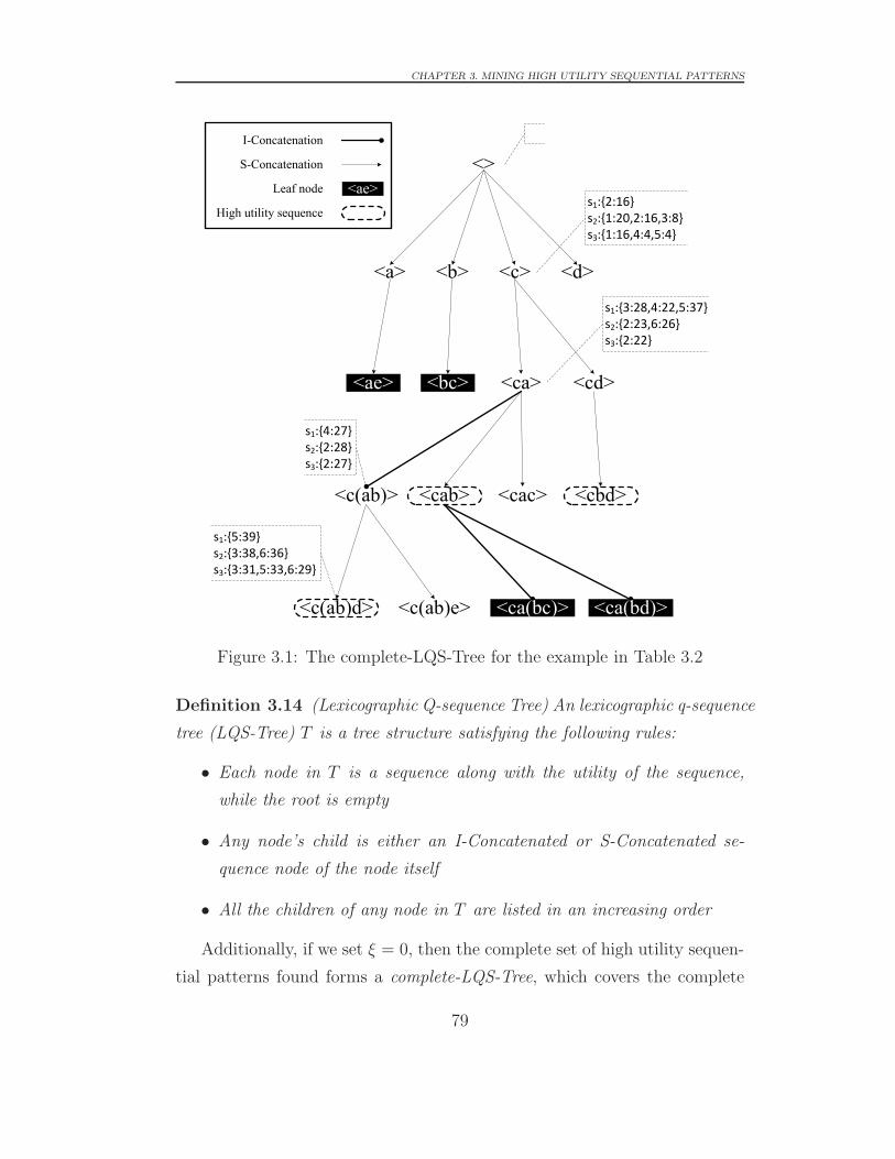
CHAPTER 3. MINING HIGH UTILITY SEQUENTIAL PATTERNS
s1:{2:16}s2:{1:20,2:16,3:8}s3:{1:16,4:4,5:4}
<>
s1:{3:28,4:22,5:37}s2:{2:23,6:26}s3:{2:22}
s1:{4:27}s2:{2:28}s3:{2:27}
s1:{5:39}s2:{3:38,6:36}s3:{3:31,5:33,6:29}
I-Concatenation
S-Concatenation
Leaf node
High utility sequence
<ae>
<a> <b> <c> <d>
<ae> <bc> <ca> <cd>
<c(ab)> <cab> <cac> <cbd>
<c(ab)d> <c(ab)e> <ca(bc)> <ca(bd)>
Figure 3.1: The complete-LQS-Tree for the example in Table 3.2
Definition 3.14 (Lexicographic Q-sequence Tree) An lexicographic q-sequence
tree (LQS-Tree) T is a tree structure satisfying the following rules:
• Each node in T is a sequence along with the utility of the sequence,
while the root is empty
• Any node’s child is either an I-Concatenated or S-Concatenated se-
quence node of the node itself
• All the children of any node in T are listed in an increasing order
Additionally, if we set ξ = 0, then the complete set of high utility sequen-
tial patterns found forms a complete-LQS-Tree, which covers the complete
79

CHAPTER 3. MINING HIGH UTILITY SEQUENTIAL PATTERNS
search space.
Figure 3.1 is example of LQS-Tree. The root is an empty q-sequence,
while the nodes in the black boxes such as 〈ae〉 are leaves in the LQS-
Tree. The bold lines and the light lines represent I-Concatenation and S-
Concatenation, respectively. Nodes within the same parent are arranged
in increasing order. Given the minimum utility ξ = 104, the high utility
sequences are marked in the dotted round-corner boxes. For example, se-
quence 〈c(ab)d〉 is a high utility sequence since its utility is 110, which is
above ξ = 104.
Given a sequence t and a utility-based sequence database S, calculatingv(t) in S is easy without any prior knowledge. For example, if we want to
calculate v(〈ca〉), we simply find all the q-subsequences in each q-sequence
that match 〈ca〉, and calculate the utilities of those q-subsequences. We
obtain v(〈ea〉) = {{8, 10}, {16, 10}, {15, 7}} and umax(〈ea〉) = 41. Once we
have umax(〈ea〉), a very natural question is, “Can any 〈ea〉’s child’s maximum
utility be calculated by simply adding the highest utility of the q-items after
〈ea〉 to umax(〈ea〉)?”. Unfortunately, the answer is no.
In frequent sequential pattern mining, the downward closure property
serves as the foundation of pattern mining algorithms. However, this prop-
erty does not hold in the high utility pattern mining problem. In Figure
3.1, umax(〈c〉) = 16 + 20 + 16 = 52, but umax(〈ca〉) = 37 + 26 + 22 = 85,
which is lower than its super-pattern. Thus, any frequent sequential pattern
mining algorithms built on this property, such as prefixspan (Pei et al. 2004)
and SPADE (Zaki 2001), cannot mine for high utility sequences. What is
more, if we check the maximum utilities of a path in the complete-LQS-Tree,
we find that the utilities of the sequential patterns 〈c〉, 〈ca〉, 〈c(ab)〉 and
〈c(ab)d〉 are 52, 85, 82 and 110, respectively. There is no such property as
monotonicity or anti-monotonicity in the maximum utilities. Therefore, it
is not surprising that given ξ > 0, the high utility sequences may not for-
m a complete-LQS-Tree. For example, only two sequences satisfy ξ = 159,
they are umax(〈d(bcf)d(bf)(adf)〉) = 163 and umax(〈d(bcf)db(adf)〉) = 159.
80

CHAPTER 3. MINING HIGH UTILITY SEQUENTIAL PATTERNS
Obviously, these two patterns cannot form a complete-LQS-Tree.
USpan consequently uses a depth-first search strategy to traverse the
LQS-Tree to search for high utility patterns. As shown in Figure 3.1, USpan
first generates the children of the root. It then takes 〈a〉 as the current node,checks whether 〈a〉 is a high utility pattern, and scans for 〈a〉’s possible
children. If 〈a〉’s first children, i.e. 〈(ab)〉, are not taken as the current node,
the same operations will apply to 〈(ab)〉. This procedure will be recursively
invoked until there is no other node in the LQS-Tree to visit.
Two important things about USpan need to be highlighted. First, know-
ing the utility of a node, how can we generate the node’s children’s utilities
by concatenating the corresponding items? The answer is in Section 3.3.2.
Then, how can we avoid checking unpromising children? We discuss this in
Section 3.3.3, which includes three different pruning strategies.
3.3.2 Concatenations
At this point, we discuss how to generate the children’s utility based on
the utility of its parent, in other words, through I-Concatenation and S-
Concatenation. For example, if we already know the “muv” of 〈c〉, as shownin Figure 3.1., I-Concatenation and S-Concatenation explain how to obtain
the “muvs” of its children such as 〈ca〉 and 〈cd〉 etc. We introduce a utility
matrix to represent the utility of a q-sequence. Table 3.3 is the utility matrix
of q-sequence s1 in Table 3.2. Each element in the matrix is either empty
(denoted as ”-”) or a tuple; the first value shows the utility of the q-item,
and the second is the utility of the remaining items in the q-sequence; we
call it remaining utility, which will be discussed in Subsection 3.3.3.
We illustrate the concatenations with q-sequence s3; other sequences can
be conducted in the same way. As shown in Figure 3.1., we use the path
“〈〉 → 〈c〉 → 〈ca〉 → 〈c(ab)〉 → 〈c(ab)d〉” as an example to demonstrate. Let
us look at the record for sequence 〈ca〉 in Table 3.3. Clearly, only sub-q-
sequence 〈c1a2〉 matches the sequence 〈ca〉, so muv(〈ca〉, s3) = {22}. Items
can either I-Concatenate or S-Concatenate to an existing pattern.
81

CHAPTER 3. MINING HIGH UTILITY SEQUENTIAL PATTERNS
Table 3.3: Utility Matrix of Q-sequence s3 in Table 3.2
items TID 1 TID 2 TID 3 TID 4 TID 5 TID 6
a (18,87) (6,55) - - - -
b - (5,50) - (10,30) - (5,2)
c (16,71) - - (4,26) (4,17) -
d (10,61) - (4,40) - (6,11) (2,0)
e - - - (5,21) (4,7) -
f - (6,44) - - - -
We start from the I-Concatenation. In the example, only items larger
than a can be I-Concatenated, i.e. entries in the rectangle from b2 to f6 are
possible items. More precisely, only b2, that is (b, 5), can be used to form the
sub-q-sequences that match the sequence 〈(be)〉. The muv of 〈c(ab)〉 is the
ending q-item utility of 〈ca〉 plus the newly added q-items’ utility b = (2, 38),
i.e. muv(〈c(ab)〉, s3) = {22 + 5} = {27}. Similarly, in s1 and s2, we have
muv(〈c(ab)〉, s1) = {27} and muv(〈c(ab)〉, s2) = {28}, as shown in Figure
3.1. Some other examples are muv(〈c(ac)〉, s2) = {39}, muv(〈c(ad)〉, s1) =
{32, 49}, muv(〈c(af)〉, s3) = {28} and so on.
S-Concatenation is a little more complicated. We continue with 〈c(ab)〉 ins3. Q-items that can be S-Concatenated to the q-subsequences are located in
the rectangle region from a3 to f6. Thus, sequences such as 〈c(ab)b〉, 〈c(ab)c〉,〈c(ab)d〉 and 〈c(ab)e〉 are the candidates. Taking 〈c(ab)d〉 as an example.
Since the only ending q-item, i.e. pivot, of 〈c(ab)〉 in s3 is b2, we now con-
catenate d to 〈c(ab)〉. In other words, u(〈c(ab)〉, b2, s3) = 27. Since d3, d5 and
d6 are located in a3 to f6, the ending q-item maximum utilities of 〈c(ab)d〉are u(〈c(ab)d〉, d3, s3) = max(27 + 4) = 31, u(〈c(ab)d〉, d5, s3) = max(27 +
6) = 33 and u(〈c(ab)d〉, d6, s3) = max(27 + 2) = 29. Therefore, we have
muv(〈c(ab)d〉, s3) = {31, 33, 29}. Similarly, we also have muv(〈c(ab)d〉, s1) ={39} and muv(〈c(ab)d〉, s2) = {38, 36}.
From the above two examples, we see that a sequence’s children’s utili-
ties can be calculated in terms of the ending q-item maximum utility. For
82

CHAPTER 3. MINING HIGH UTILITY SEQUENTIAL PATTERNS
example, to generate the utility of 〈cabd〉 based on 〈cab〉 in s3, we only need
to know the following information from 〈cab〉: i) b2, b4 and b6 are the three
last q-items of q-subsequences which match the sequence 〈cab〉, and ii) the
utilities are 27, 32 and 27 respectively. As for which q-items match c or a,
this is not important. Figure 3.2. presents the data representation in USpan.
Every sequence is stored in the memory in the form of a utility matrix. We
omit the entries in the figure for simplicity. The pivot in q-sequence 1 is the
black dot; other ending q-items are the black solid boxes on the right side of
the dot.
Sequence 2Sequence 2
Sequence 2Sequence 2
Sequence 2
1 2 3 4 5 6 7 8adefghi
Q-sequence 3
1 2 3 4 5 6 7acdfgh
Q-sequence 2
1 2 3 4 5 6 7 8 9abcdefghi
Q-sequence 1
pivot
S-Concatenationq-items
I-Concatenationq-items
Projectedq-items
Endingq-items
Sequence: (ad)fd
Figure 3.2: Data representation in USpan
3.3.3 Pruning Strategies
The above section discusses how to concatenate items to a sequence, but a
remaining issue is what kind of items are qualified to be concatenated. This
83

CHAPTER 3. MINING HIGH UTILITY SEQUENTIAL PATTERNS
section presents three utility boundaries, that is SWU(Sequence-Weighted
Utility), SPU(Sequence-Projected Utility) and SRU(Sequence-Reduced U-
tility), to calculate the upper bound of the nodes in the LQS-Tree. Corre-
spondingly, three pruning strategies in different stages of the mining process
are proposed to further select the promising items.
Sequence-Weighted Utility Pruning
The first pruning strategy is called SWU(Sequence-Weighted Utility) prun-
ing. SWU is a simple method to effectively control the width of the LQS-Tree.
As shown in Figure 3.2., those located at the left side of the pivot (inclu-
sive) are called projected q-items. Clearly, it is not possible to concatenate
these projected q items. The qualified items are at the right side of the
pivot. They are I-Concatenation items right under the pivot and the end-
ing q-items, and S-Concatenation q-items are on the right side of the pivot.
For each sequence in S, those items should be scanned and inserted into the
corresponding I-Concatenation and/or S-Concatenation lists.
Not every qualified item is a promising item. For example, s1 and s3
contain 〈c(ab)〉. If we scan the projected database, a - e are qualified to
concatenate (s1 contains a, d, f and s3 contains b, c, d, e). Assuming that
ξ = 110, b, c and e are actually unpromising, which means they cannot be
high utility patterns. Taking b as an example, the maximum utility of any
sequence containing b will be no more than the utility of s3, that is 105, so
any super-sequence of 〈c(ab)〉 concatenating with b will, if it can, make itself
a low utility pattern.
To avoid selecting the unpromising items, we propose a Sequence-Weighted
Utility (SWU) pruning strategy for the scanning subroutine. This is based on
the Sequence-weighted Downward Closure Property (SDCP), which is simi-
lar to the Transaction-weighted Downward Closure Property (TDCP) in (Liu
et al. 2005b). Before introducing SDCP, we give a definition to the Sequence-
Weighted Utility (SWU) of a sequence.
Definition 3.15 (SWU) The Sequence-Weighted Utility(SWU) of a sequence
84

CHAPTER 3. MINING HIGH UTILITY SEQUENTIAL PATTERNS
t in S is denoted and defined as SWU(t)
SWU(t) =∑
s′∼t∧s′⊆s∧s⊆Su(s) (3.3.5)
For sequence 〈a〉, since all the q-sequences s1, s2 and s3 contain the se-
quence, so SWU(〈a〉) = u(s1)+u(s2)+u(s3) = 112+117+105 = 334. Simi-
larly, SWU(〈(ac)〉) = u(s2)+u(s3) = 117+105 = 222 and SWU(〈(ac)ca〉) =u(s2) = 117.
Theorem 3.1 (Sequence-weighted Downward Closure Property) Given a utility-
based sequence database S, and two sequences t1 and t2, where t2 contains t1,
then
SWU(t2) � SWU(t1) (3.3.6)
Proof Let s2 ⊆ sj ∈ S be a subsequence matching the sequence t2. Since t2
contains t1, we know that there must be a subsequence s1 ⊆ s2 matching t1.
Therefore, a sequence containing subsequences such as s2 is a subset of that
containing s1, i.e
{sj : s2 ∼ t2 ∧ s2 ⊆ sj ∧ sj ⊆ S} ⊆ {si : s1 ∼ t1 ∧ s1 ⊆ si ∧ si ⊆ S} (3.3.7)
We derive, ∑
s2∼t2∧s2⊆sj∧sj⊆Su(sj) �
∑
s1∼t1∧s1⊆si∧si⊆Su(si) (3.3.8)
and obtain SWU(t2) � SWU(t1).
Based on Theorem 3.1, we define whether an item is “promising”. Imagine
we have a k-sequence t, a new item i concatenates to t and results in a
(k+1)-sequence t′. If SWU(t′) � ξ, we say item i is a promising item to t.
Otherwise, i is called an unpromising item. In the implementation, to test
whether an item is promising, we do not have to generate the new sequence
to test whether an item is promising. We simply add the utilities of all the
sequences; this is equal to the SWU of the new sequence.
85

CHAPTER 3. MINING HIGH UTILITY SEQUENTIAL PATTERNS
Sequence-Projected Utility
The SWU pruning strategy avoids constructing unpromising patterns into the
LQS-Tree; an Sequence-Projected Utilization (SPU) pruning strategy stops
USpan from going deeper by identifying the leaf nodes in the tree. Imagine
the following scenario: the pivots are approaching the end of q-sequences;
meanwhile, the maximum utility of the sequence is much less than ξ. The
gap is so large that even if all the utilities of the remaining q-items are
counted into the utility of the sequence, the cumulative utility still cannot
satisfy ξ. In this situation, we use the depth pruning strategy to backtrack
USpan instead of waiting to go deeper and returning with nothing.
Definition 3.16 (Sequence-Projected Utilization) The Sequence-Projected U-
tilization (SPU) of a sequence t in S is denoted and defined as SPU(t)
SPU(t) =∑
i∈s∧s∈S(urest(i, s) + up(t, s)), (3.3.9)
where i is the pivot of t in s, and
urest(i, s) =∑
i′∈s∧i≺i′u(i′) (3.3.10)
We use the notation urest(i, s) to refer to the remaining utility at q-item
i (exclusive) in q-sequence s. The calculation is simply adding up all the
utilities after the pivot. In the utility matrix, the remaining utility appears in
the second element in each entry, as shown in Table 3, e.g. urest(b1, s4) = 40,
urest(d2, s4) = 15.
Theorem 3.2 Given a utility-based sequence database S, and two sequences
t1 and t2, where t2 contains t1, then
SPU(t2) � SPU(t1) (3.3.11)
Proof Suppose we have the utility of sequence t in S, we can divide each
sequence s ∈ S into two parts from the pivots, where the pivots are in the
left part. Assume s′ ⊆ s and pivot i ∈ s′, in other words, s′ is the far left
86

CHAPTER 3. MINING HIGH UTILITY SEQUENTIAL PATTERNS
subsequence in s that matches t. t’s offspring can be only concatenated from
the right side of the pivot. Correspondingly, it is easy to understand that
the maximum utilities of the concatenated items are no more than urest(i, s).
Hence, the utility of any item concatenated from s is no more than urest(i, s)+
u(s′). Similarly, the highest utility of other sequences in S can be calculated
in the same way. Therefore, we have the theorem.
Based on Theorem 3.2, if the utility upper bound, i.e. the sum of re-
maining utilities and utilities of far left subsequences, is less than ξ, we can
simply stop USpan from going deeper and backtrack the search procedure.
Sequence-Reduced Utility
In this part, we provide a tighter sequence boundary and a novel pruning
strategy. The following example illustrates the problem.
Assume that ξ = 144. By concatenating a to 〈〉, it results in 〈a〉 with u-
tility 66. Scanning 〈a〉’s children with SPU , that is the pivot utility plus the
rest utility, we have the following S-Concatenation items and the correspond-
ing SWUs: {c : 310, b : 310, a : 310, f : 310, e : 222}. Let a S-Concatenate to
〈a〉, we have 〈aa〉 with the utility of 55.
Having the status of 〈aa〉 in S, next we scan for items that are promising
to be concatenated. Instead of using the SWU as the boundary, we calculate
SPUs of the items. The SPU(〈aa〉) in the 3 q-sequences are SPU(〈aa〉, s1) =75, SPU(〈aa〉, s2) = 18 and SPU(〈aa〉, s1) = 79. Therefore, the items and
their SPUs are {a : 75, b : 154, c : 79, d : 154, e : 79, f : 75}. Note that as
only b and d’ SPUs satisfy the ξ, they are identified as the promising items.
The others should be removed from the S-Concatenation list.
Let us revisit a, c, e and f . Taking a as an example, a is not promising
because the utilities of all of 〈aaa〉’s offspring will be no more than ξ. In other
words, one can remove some a’s utilities from 〈aa〉’s projected database, and
the same be done for c, e and f . The “dead” q-items are {a4, a5, f4, f5} in
s1 and {c4, c5, e4, e5} in s3. Since these items can be no longer appended
87

CHAPTER 3. MINING HIGH UTILITY SEQUENTIAL PATTERNS
to 〈aa〉 and its offspring, we remove them from the projected q-sequences.
Therefore, the updated SPUs in s1, s2 and s3 are 39, 18 and 62 respectively.
Since the SPUs of the projected q-sequences are reduced, a new scan
is needed because items with the updated SPUs may not satisfy ξ any
more. Recalculating the SPUs of b and d, they are {b : 101, d : 101},which do not satisfy ξ = 144. Therefore, b and d are also removed from the
S-Concatenation list. Until now, a, b, c, d, e, f , which are identified as promis-
ing S-Concatenation items by SWU , are actually unpromising according to
the analysis.
Until now, one can see that the SPU , as the boundary of concatenation
items, is not tight enough. The utilities of the q-items located in the rest
q-sequences are not always counted into urest. We now present the formal
definitions of the boundary and the pruning strategy below.
Definition 3.17 (Sequence-Reduced Utility) Let I = {i1, i2, ..., in} be a set
of distinct items, and B,W ⊆ I, where B is named as blacklist and W is
named as whitelist, and B ∪ W = I, B ∩W = ∅. Given a sequence t, a q-
sequence s = 〈l1l2...ln〉. Suppose s � t, let ip be the pivot of t in s and ip ∈ lm,
where 1 ≤ m ≤ n. The SRU(Sequence-Reduced Utility) of a sequence t in s
is denoted and defined as SRU(t, s)
SRU(t, s) =up(t, s) +∑
ip≺i′∧i′∈lmu(i′)
+
n∑
k=m+1
∑
i′∈lk∧i′∈Wu(i′)
Given an item i, the SRU of i in t’s projection database is denoted and
defined as
SRU(i, t) =∑
{SRU(t, s)|i′ ∼ i ∧ i′ ∈ lk ∧ s ∈ S} (3.3.12)
Item i ∈ W if and only if SRU(i, t) ≥ ξ.
88
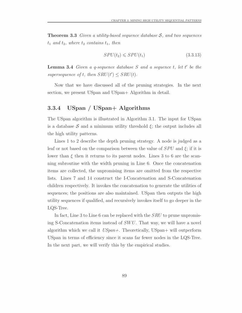
CHAPTER 3. MINING HIGH UTILITY SEQUENTIAL PATTERNS
Theorem 3.3 Given a utility-based sequence database S, and two sequences
t1 and t2, where t2 contains t1, then
SPU(t2) � SPU(t1) (3.3.13)
Lemma 3.4 Given a q-sequence database S and a sequence t, let t′ be the
supersequence of t, then SRU(t′) ≤ SRU(t).
Now that we have discussed all of the pruning strategies. In the next
section, we present USpan and USpan+ Algorithm in detail.
3.3.4 USpan / USpan+ Algorithms
The USpan algorithm is illustrated in Algorithm 3.1. The input for USpan
is a database S and a minimum utility threshold ξ; the output includes all
the high utility patterns.
Lines 1 to 2 describe the depth pruning strategy. A node is judged as a
leaf or not based on the comparison between the value of SPU and ξ; if it is
lower than ξ then it returns to its parent nodes. Lines 3 to 6 are the scan-
ning subroutine with the width pruning in Line 6. Once the concatenation
items are collected, the unpromising items are omitted from the respective
lists. Lines 7 and 14 construct the I-Concatenation and S-Concatenation
children respectively. It invokes the concatenation to generate the utilities of
sequences; the positions are also maintained. USpan then outputs the high
utility sequences if qualified, and recursively invokes itself to go deeper in the
LQS-Tree.
In fact, Line 3 to Line 6 can be replaced with the SRU to prune unpromis-
ing S-Concatenation items instead of SWU . That way, we will have a novel
algorithm which we call it USpan+. Theoretically, USpan+ will outperform
USpan in terms of efficiency since it scans far fewer nodes in the LQS-Tree.
In the next part, we will verify this by the empirical studies.
89

CHAPTER 3. MINING HIGH UTILITY SEQUENTIAL PATTERNS
Algorithm 3.1: USpan(t,muv(t))
Input: A sequence t, t’s utility muv(t), a utility-based sequence
database S, the minimum utility threshold ξ
Output: All high utility sequential patterns
1 if p is pruned by SPU then
2 return
3 scan the projected database S(muv(t)) once to:;
4 a).put I-Concatenation items into ilist, or;
5 b).put S-Concatenation items into slist;
6 remove unpromising items in ilist and slist;
7 for item i in ilist do
8 (t′, muv(t′)) ← I-Concatenate(p,i);
9 if umax(t′) � ξ then
10 output t′;
11 for item i in slist do
12 (t′, muv(t′)) ← S-Concatenate(p,i);
13 if umax(t′) � ξ then
14 output t′;
15 return;
90

CHAPTER
3.MIN
ING
HIG
HUTIL
ITY
SEQUENTIA
LPATTERNS
Characteristics DS1 DS2 DS3 DS4 DS5 DS6
Average itemset per sequence C 10 8 4.3 4.7 10 1
Average items per itemset T 2.5 2.5 4.83 1 1 7.22
Average itemsets in maximum sequences S 10 6 - - - -
Average items in maximum sequences I 2.5 2.5 - - - -
Number of sequences D 100k 10k 7,824 989,818 7,631 1,112,949
Number of different items N 1k 10k 1,559 17 3,340 46,086
The maximum length of a sequence 111 131 243 14,795 379 170
The frequency of the most frequent item 1,046 446 143 940,469 3,766 63,818
Table 3.4: Characteristics of the Synthetic Datasets
91

CHAPTER 3. MINING HIGH UTILITY SEQUENTIAL PATTERNS
3.4 Experiments
In this section, we evaluate the performance of the proposed algorithms. We
implemented our algorithms in C++ of Microsoft Visual Studio 2010. All
experiments are conducted on a virtual machine in a server with Intel Xeon
CPU of 3.10GHz, 8GB memory and Windows 7 operating system.
Extensive experiments on two synthetic and four real world datasets are
used. The characteristics of the datasets are shown in Table 3.4. DS1 and
DS2 are two synthetic datasets generated by IBM data generator (Agrawal &
Srikant 1994), and DS3 to DS6 are real world datasets. DS3 is a real dataset
from the Microsoft Food Mart 2008 database (Microsoft 2008). The dataset
shows the retail shopping transactions in 1998. Each customer has a sequence
of shopping records containing information on product ID, the amount of the
product and its price and cost. DS4 is a real web click stream dataset from
UCI (Heckerman 1999). This data describes the page visits of users who
visited msnbc.com on September 28, 1999. Visits are recorded at the lev-
el of URL category (17 types) and are recorded in time order. DS5 is the
BMS-WebView-2 dataset from the KDDCUP 2000 (SIGKDD 2000). It con-
tains clickstream and purchase data from Gazelle.com, a legwear and legcare
web retailer. DS6 is known as the “Chainstore” dataset which we download-
ed from Nu-MineBench 2.0 (Pisharath, Liu, Ozisikyilmaz, Narayanan, Liao,
Choudhary & Memik 2005). Of all the datasets, only DS3 and DS6 contain
the profits of the items. We use a log-normal distribution with μ = log(20)
and σ2 = 1.0 from 1 to 100 to generate the quality table, and the quantities
of the items are randomly generated between 1 and 10.
As discussed in Section 3.3.4, USpan used SWU and SPU for pruning un-
promising candidates while SRU and SPU are used in USpan+. To compare
the pruning strategies, we also implemented the pruning strategies SWU,
SPU and SRU singly and respectively. The details of these techniques are
discussed in Section 3.3.3. To evaluate the impact of the high utility se-
quential patterns, we downloaded prefixspan (Pei et al. 2004) executable to
extract the frequent sequential patterns from DS1 to DS6. Since the frequent
92

CHAPTER 3. MINING HIGH UTILITY SEQUENTIAL PATTERNS
patterns do not contain the utilities, we further implement a utility requestor
to calculate their utilities from the databases. The requestor’s input is the
output of the prefixspan, and the output is the sequential patterns with the
utilities.
3.4.1 Performance Evaluation
We conduct intensive experiments to evaluate the performance of USpan,
USpan+ and the three pruning strategies in terms of the computational cost
(Figure 5.3) and the number of high utility patterns (Figure 5.5 ). Of the
strategies, SWU and SRU reduce the width of the LQS-Tree and SPU con-
trols the depth. We did not compare the naive approach without a pruning
strategy since the complete-LQS-Tree is too large to mine.
The execution time of mining high utility sequential patterns on DS1 to
DS7 is shown in Figure 5.3. When the minimum utility threshold decreases
linearly, the costs grow exponentially since many more high utility sequen-
tial patterns are obtained. Generally, USpan+ outperforms all others since
USpan+ incorporates the best strategies. It’s up to 1000+ times (in Figure
5.3(d)) faster than the slowest algorithm.
Speaking of the width pruning strategies, we can observe that SRU is
faster than SWU when ξ is high. When ξ is low, these two width pruning
strategies show a similar performance, for example ξ = 0.0758% in Figure
5.3(a), ξ = 0.0338% in Figure 5.3(c) and ξ = 0.1735% in Figure 5.3(d). This
is because more candidates can be pruned by SRU when ξ is high. Multi-
scanning reduces the size of projection databases significantly. However,
lower ξ means more patterns can be discovered, which means SRU may
refresh the project database much less than when ξ is high. In other words,
SRU scans only one time in contrast to SWU.
The depth pruning method SPU is very sensitive to the minimum utility.
When the threshold is high, the pruning is very effective, because it only
goes deeper when there is a higher remaining utility value. It can totally
ignore invalid searches by pruning patterns whose pivots appear at the end
93

CHAPTER 3. MINING HIGH UTILITY SEQUENTIAL PATTERNS
0.075 0.0755 0.076 0.0765 0.077101
102
103
104
105
Tim
e(Se
c.)
Threshold (%)
SWUSPUSRUUSpanUSpan+
(a) DS1
0.075 0.08 0.085 0.09 0.095 0.1 0.105102
103
104
Tim
e(Se
c.)
Threshold (%)
SWUSPUSRUUSpanUSpan+
(b) DS2
0.1731 0.1732 0.1733 0.1734 0.1735 0.1736 0.1737 0.1738 0.1739100
101
102
103
104
105
Tim
e(Se
c.)
Threshold (%)
SWUSPUSRUUSpanUSpan+
(c) DS3
0 0.2 0.4 0.6 0.8 1101
102
103
104
Tim
e(Se
c.)
Threshold (%)
SWUSPUSRUUSpanUSpan+
(d) DS4
0.0572 0.0574 0.0576 0.0578 0.058 0.0582 0.0584102
103
104
Tim
e(Se
c.)
Threshold (%)
SWUSPUSRUUSpanUSpan+
(e) DS5
0.1 0.15 0.2 0.25 0.3 0.35102
103
104
105
Tim
e(Se
c.)
Threshold (%)
SWUSPUSRUUSpanUSpan+
(f) DS6
Figure 3.3: Performance comparison
94
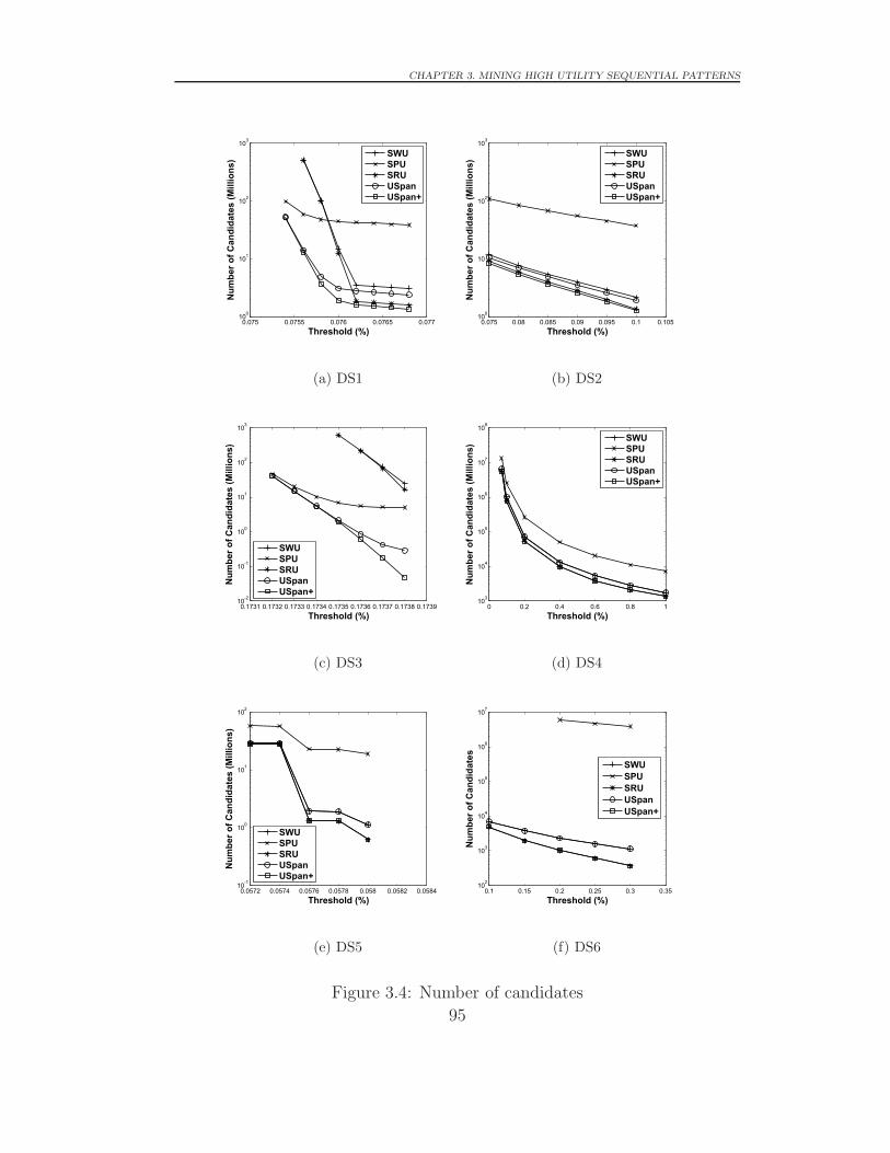
CHAPTER 3. MINING HIGH UTILITY SEQUENTIAL PATTERNS
0.075 0.0755 0.076 0.0765 0.077100
101
102
103
Num
ber o
f Can
dida
tes
(Mill
ions
)
Threshold (%)
SWUSPUSRUUSpanUSpan+
(a) DS1
0.075 0.08 0.085 0.09 0.095 0.1 0.105100
101
102
103
Num
ber o
f Can
dida
tes
(Mill
ions
)
Threshold (%)
SWUSPUSRUUSpanUSpan+
(b) DS2
0.1731 0.1732 0.1733 0.1734 0.1735 0.1736 0.1737 0.1738 0.173910-2
10-1
100
101
102
103
Num
ber o
f Can
dida
tes
(Mill
ions
)
Threshold (%)
SWUSPUSRUUSpanUSpan+
(c) DS3
0 0.2 0.4 0.6 0.8 1103
104
105
106
107
108
Num
ber o
f Can
dida
tes
(Mill
ions
)
Threshold (%)
SWUSPUSRUUSpanUSpan+
(d) DS4
0.0572 0.0574 0.0576 0.0578 0.058 0.0582 0.058410-1
100
101
102
Num
ber o
f Can
dida
tes
(Mill
ions
)
Threshold (%)
SWUSPUSRUUSpanUSpan+
(e) DS5
0.1 0.15 0.2 0.25 0.3 0.35102
103
104
105
106
107
Num
ber o
f Can
dida
tes
Threshold (%)
SWUSPUSRUUSpanUSpan+
(f) DS6
Figure 3.4: Number of candidates
95
CHAPTER 3. MINING HIGH UTILITY SEQUENTIAL PATTERNS
of sequences. However, when ξ decreases, the search space in the LQS-Tree
grows exponentially. In contrast, width pruning is more stable with the
decrease of the threshold. The reason is that width pruning always prevents
unpromising items from getting into the concatenation lists. It can control
the width of the trees very well, however it cannot control whether the current
sequence is promising until it reaches the very end of the LQS-Tree. The
combination of both width and depth pruning strategies leads to extremely
improved efficiency compared to either of them. The combination can result
in up to eight times the difference in execution time, because the two kinds
of pruning strategies can compensate for the shortcomings of each other.
In addition, since the high utility sequential pattern mining algorithm in
(Ahmed, Tanbeer, Jeong & Lee 2010) is essentially based on width-pruning,
the experimental results indirectly show that USpan and USpan+ are much
more efficient.
Figure 5.5 shows the candidates generated by the proposed algorithms.
Here, the number of candidates means the number of nodes in the LQS-
Tree, which is also the same as the number of projection databases. From
these results, one can tell more candidates require more running time, which
explains the trends in Figure 5.3. Notice that in Figure 3.4(e) and Figure
3.4(f), the candidate counts of SWU and USpan, SRU and USpan+ are
exactly the same, but in Figure 5.3(e) and Figure 5.3(f), their runtimes are
different. This is because the SPU strategy prunes the leaves in the LQS-
Tree. Taking USpan and SWU as an example. Suppose both of them reach
a leaf node in LQS-Tree. In Algorithm 3.1, USpan returns at line 2 while
SWU has to execute line 3, which is a very costly subroutine, to reach line
15. This also explains why USpan+ outperforms SRU even if they have the
same number of candidates.
3.4.2 Pattern Length Distributions
In this part, we show pattern length distributions of the top 1000 and 2000
of frequency-based and utility-based sequential patterns from the datasets
96

CHAPTER 3. MINING HIGH UTILITY SEQUENTIAL PATTERNS
respectively, as shown in Figure 3.5. The frequent patterns are extracted by
prefixspan (Pei et al. 2004). The X axis refers to the length of the patterns
and Y refers to the number of patterns at the lengths.
Figure 3.5 shows that the discovered patterns under the two different
frameworks can be very different. The frequency-based patterns are mainly
distributed in the short-length area compared with the utility-based patterns.
For example, in Figure 3.5(a) and Figure 3.5(b), the utility-based patterns
are generally longer than the frequency-based ones. This reveals that the
Apriori property which holds in the frequency/support framework does not
hold in utility sequence mining. In Figure 3.5(e) and Figure 3.5(f), both
types have similar length patterns, but the longer utility-based patterns are
clearly more than those of the frequency-based ones. In Figure 3.5(c), the
utility-based patterns are extracted from a small group of sequences from the
database, which explains why high utility patterns are distributed in a very
narrow range.
3.4.3 Utility Comparison with Frequent Pattern Min-
ing
This experiment tests the utility difference between the patterns identified by
USpan and that the patterns identified by prefixspan (Pei et al. 2004). For
each of the datasets, we sort the top 2000 frequent patterns according to their
frequencies. Then we calculated the patterns’ utilities from the database. On
the other hand, we sort the top 2000 high utility patterns according to their
utilities. In the figures, the X axis refers to the top n number of frequent vs.
high-utility patterns selected from the two groups, while the Y axis shows
the sum of the relative utilities of the top n patterns. The results show that
USpan can identify higher utility patterns more efficiently, and it can extract
top patterns with higher average utility per pattern.
97

CHAPTER 3. MINING HIGH UTILITY SEQUENTIAL PATTERNS
0 5 10 15 20 25 300
200
400
600
800
1000
1200
1400
# of
Pat
tern
s
Pattern Length
U 1000F 1000U 2000F 2000
(a) DS1
0 5 10 15 200
200
400
600
800
1000
1200
# of
Pat
tern
s
Pattern Length
U 1000F 1000U 2000F 2000
(b) DS2
0 50 100 150 200 2500
200
400
600
800
1000
1200
1400
1600
# of
Pat
tern
s
Pattern Length
U 1000F 1000U 2000F 2000
(c) DS3
0 5 10 15 20 25 30 350
50
100
150
200
250
300
350
400
450
# of
Pat
tern
s
Pattern Length
U 1000F 1000U 2000F 2000
(d) DS4
0 2 4 6 8 100
100
200
300
400
500
600
# of
Pat
tern
s
Pattern Length
U 1000F 1000U 2000F 2000
(e) DS5
1 1.5 2 2.5 3 3.5 40
200
400
600
800
1000
1200
# of
Pat
tern
s
Pattern Length
U 1000F 1000U 2000F 2000
(f) DS6
Figure 3.5: Pattern length distributions
98

CHAPTER 3. MINING HIGH UTILITY SEQUENTIAL PATTERNS
0 500 1000 1500 200040
60
80
100
120
140
160
180
200
220
Sum
Util
ity o
f Top
# P
atte
rns
(%)
Top # Patterns
UtilityFrequency
(a) DS1
0 500 1000 1500 20000
50
100
150
200
250
300
350
Sum
Util
ity o
f Top
# P
atte
rns
(%)
Top # Patterns
UtilityFrequency
(b) DS2
0 500 1000 1500 20000
50
100
150
200
250
300
350
Sum
Util
ity o
f Top
# P
atte
rns
(%)
Top # Patterns
UtilityFrequency
(c) DS3
0 500 1000 1500 2000400
600
800
1000
1200
1400
1600
1800
2000
2200
Sum
Util
ity o
f Top
# P
atte
rns
(%)
Top # Patterns
UtilityFrequency
(d) DS4
0 500 1000 1500 20000
100
200
300
400
500
600
700
Sum
Util
ity o
f Top
# P
atte
rns
(%)
Top # Patterns
UtilityFrequency
(e) DS5
0 500 1000 1500 200020
30
40
50
60
70
80
Sum
Util
ity o
f Top
# P
atte
rns
(%)
Top # Patterns
UtilityFrequency
(f) DS6
Figure 3.6: High utility vs. frequent sequential patterns
99
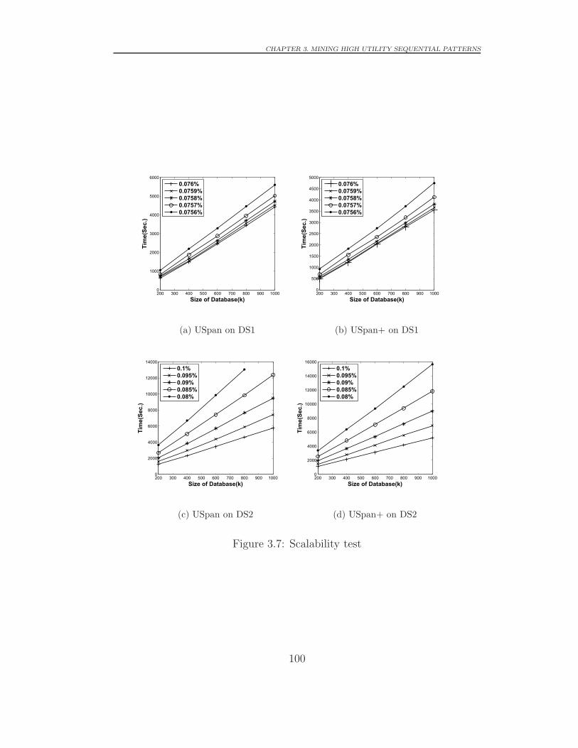
CHAPTER 3. MINING HIGH UTILITY SEQUENTIAL PATTERNS
200 300 400 500 600 700 800 900 10000
1000
2000
3000
4000
5000
6000
Tim
e(Se
c.)
Size of Database(k)
0.076%0.0759%0.0758%0.0757%0.0756%
(a) USpan on DS1
200 300 400 500 600 700 800 900 10000
500
1000
1500
2000
2500
3000
3500
4000
4500
5000
Tim
e(Se
c.)
Size of Database(k)
0.076%0.0759%0.0758%0.0757%0.0756%
(b) USpan+ on DS1
200 300 400 500 600 700 800 900 10000
2000
4000
6000
8000
10000
12000
14000
Tim
e(Se
c.)
Size of Database(k)
0.1%0.095%0.09%0.085%0.08%
(c) USpan on DS2
200 300 400 500 600 700 800 900 10000
2000
4000
6000
8000
10000
12000
14000
16000
Tim
e(Se
c.)
Size of Database(k)
0.1%0.095%0.09%0.085%0.08%
(d) USpan+ on DS2
Figure 3.7: Scalability test
100

CHAPTER 3. MINING HIGH UTILITY SEQUENTIAL PATTERNS
3.4.4 Scalability Test
The scalability test is conducted to test the performance of both USpan and
USpan+ on large-scale datasets. Figure 3.4.4 shows the results on datasets
DS1 and DS2 in terms of different data sizes: 200K to 1000K sequences are
extracted from DS1 and DS2, by setting ξ = 0.0756% to ξ = 0.076% on
DS1 and ξ = 0.08% to ξ = 0.1% on DS2.
On both datasets and algorithms, the execution times are exactly linear
with the number of transactions, as shown in Figure 3.4.4. USpan stores
the whole dataset, and the running time is directly related to the size of the
LQS-Tree. Since increasing the size of the datasets only requires more time
on each node but not depth and width of the tree, the runtime grows linearly.
3.5 Summary
Sequential pattern mining is a very important issue in data mining and ma-
chine learning. Most traditional sequence mining focus on extracting pat-
terns in the frequency/support framework which do not show business value
and impact, and thus are not actionable for business decision-making. The
introduction of “utility” not only brought valuable knowledge in sequence
analysis, but also new problems and challenges. First, the absence of the
Apriori Property in high utility sequence analysis makes the mining process
fundamentally different with frequent sequence mining. Novel structures and
algorithms are need to be designed to improve the performance and scala-
bility, and mining on platforms such as MapReduce from industry level big
data. Second, the measurements of a pattern utility in a sequence could be
different. For example, in (Ahmed, Tanbeer, Jeong & Lee 2010), the authors
define the utility of a pattern as the sum of “all distinct occurrences” in a
sequence. Different utility calculation definitions would lead to completely
different utility bounds, properties and pruning strategies. Third, accord-
ing to our experience in mining the utility sequence database, the come-out
patterns also suffer from a large amount of redundancy similar to the fre-
101

CHAPTER 3. MINING HIGH UTILITY SEQUENTIAL PATTERNS
quent pattern mining . Many patterns look very similar to each other. The
challenge here is to explore approaches and algorithms which could efficient-
ly and effectively summarize the patterns, and lose the smallest amount of
information as well.
In this chapter, we have provided a systematic statement of a generic
framework which defines calculations of the utility of a single item, an item-
set, a sequence and a sequence database. Then, we specified a naive case from
the framework which uses the maximum utility calculation to extract high
utility patterns. Based on this, we presented our solutions including three
utility bounds and the corresponding pruning strategies, and two efficient
algorithms USpan and USpan+ were proposed. Substantial experiments on
both synthetic and real datasets have shown that the proposed algorithm-
s can efficiently identify high utility sequences in large-scale data with low
minimum utility.
102

Chapter 4
Top-K High Utility Sequential
Pattern Mining
4.1 Introduction
Frequent sequential pattern mining (Agrawal & Srikant 1995), as one of the
fundamental research topics in data mining, discovers frequent subsequences
in sequence databases. It is very useful for handling order-based business
problems, and has been successfully adopted to various domains and ap-
plications such as complex behavior analysis and gene sequence analysis
(Mabroukeh & Ezeife 2010, Pei et al. 2004, Ayres et al. 2002, Zaki 2001). In
the frequency-based framework for typical sequence analysis, the downward
closure property (also known as Apriori property) (Agrawal & Srikant 1994)
plays a fundamental role in identifying frequent sequential patterns.
4.1.1 Top-K-based Mining
In fact, the classic frequency/support based pattern mining also faces the
same challenge. Accordingly, the concept of extracting top-k patterns has
been proposed in (Han et al. 2002, Tzvetkov et al. 2005, Cheung & Fu 2004,
Chuang et al. 2008) to select the patterns with the highest frequency. In the
top-k frequent pattern mining, instead of letting a user specify a minimum
103

CHAPTER 4. TOP-K HIGH UTILITY SEQUENTIAL PATTERN MINING
support threshold, the top-k pattern selection algorithms allow a user to set
the number of top-k high frequency patterns to be discovered. This makes
it much easier and more intuitive and practical than determining a mini-
mum support; also the determination of k by a user is more straightforward
than considering data characteristics, which are often invisible to users, for
choosing a proper threshold.
The ease for users to determine k does not indicate the simplicity of
developing an efficient algorithm for selecting top-k high utility sequential
patterns. In the utility framework, TKU (Wu et al. 2012) is the only method
for mining top-k high utility itemsets, to the best of our knowledge. No work
is reported on mining top-k high utility sequences. There is significant differ-
ence between top-k utility itemset mining and top-k utility sequence mining
in which the order between itemsets is considered. In fact, the problem of
top-k high utility sequence mining is much more challenging than mining
top-k high utility itemsets. First, as with high utility itemset mining, the
downward closure property does not hold in the utility-based sequence min-
ing. This means that the existing top-k frequent sequential pattern mining
algorithms (Tzvetkov et al. 2005) cannot be directly applied. Second, com-
pared to top-k high utility itemset mining (Wu et al. 2012), utility-based
sequence analysis faces the critical combinational explosion and computa-
tional complexity caused by sequencing between itemsets. This means that
the techniques in (Wu et al. 2012) cannot be directly transferred to top-k high
utility sequential pattern mining either. Third, since the minimum utility is
not given in advance, the algorithm essentially starts the searching from 0
minimum support. This not only incurs very high computational costs, but
also the challenge of how to raise the minimum threshold without missing
any top-k high utility sequences.
4.1.2 Research Contributions
To address the above challenges, this chapter proposes an efficient algorithm
to identify Top-k Utility Sequences (TUS). The contributions of this work
104

CHAPTER 4. TOP-K HIGH UTILITY SEQUENTIAL PATTERN MINING
are as follows.
• We propose a novel framework for extracting the top-k high utility
sequential patterns. A baseline algorithm TUSNaive is provided ac-
cordingly.
• Two strategies are proposed for effectively raising the thresholds at
different stages of the mining process.
• Substantial experiments on both synthetic and real datasets show that
the TUS algorithm can efficiently identify top-k high utility sequences
from large scale data with large k.
The remainder of the chapter is organized as follows. Section 4.2 pro-
poses a sequence utility framework and defines the problem of mining top-k
high utility sequential patterns. Section 4.3 details the TUS algorithm. Ex-
perimental results and evaluation are presented in Section 4.4. Section 4.5
concludes the work.
4.2 Problem Statement
Let I = {i1, i2, ..., in} be a set of distinct items. A utility item, or u-item,
is an ordered pair (i, u), where i ∈ I represents an item and u is a positive
number representing the utility of i, e.g. the profit of i. A utility itemset, or
u-itemset, consists of no less than one u-item, which is denoted and defined
as l = [(ij1 , u1)(ij2, u2)...(ijn′ , un′)], where (ijk , uk) is a u-item for 1 � k � n′,
and ∀k1, k2, where 1 � k1, k2 � n′ and k1 = k2, ijk1 = ijk2 . For brevity, the
brackets are omitted if a u-itemset has only one u-item. Since the items in
an itemset can be listed in any order. Without loss of generality, we assume
that u-items are listed in the alphabetical order. A utility sequence, or u-
sequence, is an ordered list of u-itemsets, which is denoted and defined as
s = 〈l1l2 ... lm〉, where lk(1 � k � m) is a u-itemset. A u-sequence database
S consists of sets of tuples 〈sid, s〉, where sid is a unique identifier of the
u-sequence s.
105

CHAPTER 4. TOP-K HIGH UTILITY SEQUENTIAL PATTERN MINING
Table 4.1: U-sequence Database
SID TID Transactions TU SU
1 1 (a,6)(d,8)(e,1) 15
112
1 2 (b,10)(c,16)(f,2) 28
1 3 (a,12)(d,4) 16
1 4 (a,6)(b,5)(f,3) 14
1 5 (a,21)(d,12)(f,6) 39
2 1 (c,20)(d,4) 24
117
2 2 (a,3)(b,5)(c,16)(f,5) 29
2 3 (c,8)(d,10)(e,3) 21
2 4 (f,6) 6
2 5 (b,20)(e,1)(f,1) 22
2 6 (a,6)(d,8)(f,1) 15
3 1 (a,18)(c,16)(d,10) 44
105
3 2 (a,6)(b,5)(f,6) 17
3 3 (d,4) 4
3 4 (b,10)(c,4)(e,5) 19
3 5 (c,4)(d,6)(e,4) 14
3 6 (b,5)(d,2) 7
Table 4.1 illustrates a u-sequence database containing three u-sequences.
In sid = 1 u-sequence, (a, 6), (d, 8), (e, 1) etc. are u-items; [(a, 6)(d, 8)(e, 1)]
is a u-itemset with three u-items. For convenience, in this chapter, “se-
quence” refers to ordered itemsets without utilities, i.e. the same meaning
in frequent sequence mining; similarly, “item” and “itemset” do not involve
quantity either. We use “u-” to name an object associated with utility. We
denote the sid = 1 u-sequence in Table 4.1 as s1; other u-sequences are
numbered accordingly. Additionally, a (u-)sequence is called l-(u-)sequence
i.e., its length is l iff there are l (u-)items in the (u-)sequence; the size of a
(u-)sequence is the number of (u-)itemsets in the (u-)sequence. For example,
s1 is a 14-u-sequence, s2 and s3 are 16-u-sequence and 15-u-sequence respec-
106
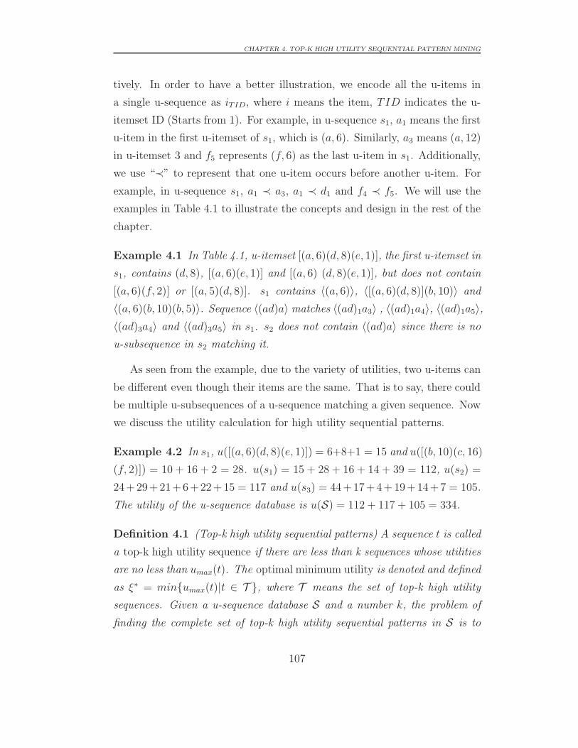
CHAPTER 4. TOP-K HIGH UTILITY SEQUENTIAL PATTERN MINING
tively. In order to have a better illustration, we encode all the u-items in
a single u-sequence as iTID, where i means the item, TID indicates the u-
itemset ID (Starts from 1). For example, in u-sequence s1, a1 means the first
u-item in the first u-itemset of s1, which is (a, 6). Similarly, a3 means (a, 12)
in u-itemset 3 and f5 represents (f, 6) as the last u-item in s1. Additionally,
we use “≺” to represent that one u-item occurs before another u-item. For
example, in u-sequence s1, a1 ≺ a3, a1 ≺ d1 and f4 ≺ f5. We will use the
examples in Table 4.1 to illustrate the concepts and design in the rest of the
chapter.
Example 4.1 In Table 4.1, u-itemset [(a, 6)(d, 8)(e, 1)], the first u-itemset in
s1, contains (d, 8), [(a, 6)(e, 1)] and [(a, 6) (d, 8)(e, 1)], but does not contain
[(a, 6)(f, 2)] or [(a, 5)(d, 8)]. s1 contains 〈(a, 6)〉, 〈[(a, 6)(d, 8)](b, 10)〉 and
〈(a, 6)(b, 10)(b, 5)〉. Sequence 〈(ad)a〉 matches 〈(ad)1a3〉 , 〈(ad)1a4〉, 〈(ad)1a5〉,〈(ad)3a4〉 and 〈(ad)3a5〉 in s1. s2 does not contain 〈(ad)a〉 since there is no
u-subsequence in s2 matching it.
As seen from the example, due to the variety of utilities, two u-items can
be different even though their items are the same. That is to say, there could
be multiple u-subsequences of a u-sequence matching a given sequence. Now
we discuss the utility calculation for high utility sequential patterns.
Example 4.2 In s1, u([(a, 6)(d, 8)(e, 1)]) = 6+8+1 = 15 and u([(b, 10)(c, 16)
(f, 2)]) = 10 + 16 + 2 = 28. u(s1) = 15 + 28 + 16 + 14 + 39 = 112, u(s2) =
24+29+21+6+22+15 = 117 and u(s3) = 44+17+4+19+14+7 = 105.
The utility of the u-sequence database is u(S) = 112 + 117 + 105 = 334.
Definition 4.1 (Top-k high utility sequential patterns) A sequence t is called
a top-k high utility sequence if there are less than k sequences whose utilities
are no less than umax(t). The optimal minimum utility is denoted and defined
as ξ∗ = min{umax(t)|t ∈ T }, where T means the set of top-k high utility
sequences. Given a u-sequence database S and a number k, the problem of
finding the complete set of top-k high utility sequential patterns in S is to
107

CHAPTER 4. TOP-K HIGH UTILITY SEQUENTIAL PATTERN MINING
discover all the itemsets whose utilities are no less than ξ∗ in S.
Example 4.3 Suppose the desired k number of high utility sequences is set to
7, the top 7 high utility sequences in Table I are shown in Table 4.2. The op-
timal minimum utility threshold ξ∗ = min{151, 152, 152, 156, 156, 159, 163}=151. If k is set to 3, then only sequences 〈d(bcf)d(bf)(adf)〉 and 〈d(bcf)db(adf)〉are obtained, and ξ∗ = 159. The reason of excluding 〈d(bc)d(bf)(adf)〉 and
〈d(bcf)d(bf)(ad)〉 is to control the number of the candidates no more than k
= 3.
Table 4.2: Top 7 High Utility Sequences in Table 4.1
ID Top-k high utility SU
1 〈d(bcf)d(bf)(adf)〉 163
2 〈d(bcf)db(adf)〉 159
3 〈d(bc)d(bf)(adf)〉 156
4 〈d(bcf)d(bf)(ad)〉 156
5 〈d(bc)db(adf)〉 152
6 〈d(bcf)db(ad)〉 152
7 〈(bcf)d(bf)(adf)〉 151
4.3 The TUS Algorithm
In the previous section, we define the top-k high utility sequential pattern
mining framework. In this section, we specify and present an efficient algo-
rithm, TUS, for mining top-k high utility sequential patterns. Firstly, we
present a baseline approach named TUSNaive. Then we present a tight util-
ity boundary for sequences, which substantially reduces the search space. In
the end, we provide a very efficient pre-insertion strategy, which effectively
raises the minimum utility threshold.
108

CHAPTER 4. TOP-K HIGH UTILITY SEQUENTIAL PATTERN MINING
4.3.1 TUSNaive: The Baseline Algorithm
Here we present a baseline algorithm called TUSNaive to extract the top-k
sequences with the highest utilities. Instead of using a user specified mini-
mum utility, TUSNaive engages a structure named TUSList to maintain the
top-k high utility sequences on-the-fly.
TUSList is a fixed-size sorted list which is used to maintain the top-k high
utility sequential patterns dynamically, and a minimum utility ξ of it is set
to prune the unpromising candidates in the mining process. The mechanism
can be briefed as follows. Initially, the TUSList is empty and ξ is set to 0.
In this stage, whenever a candidate sequence comes, it will be inserted into
TUSList, and ξ stays on 0. Once the k candidates are found, ξ is raised to
the utility of the last candidate (i.e. the least utility candidate) in TUSList.
After that, a candidate satisfying ξ is inserted into TUSList, then the least
utility candidate(s) will be eliminated. ξ is thereafter raised to utility of the
updated last candidate. The process continues until no candidate matches ξ,
and those remain in the TUSList are the target patterns. The pseudo code
of TUSNaive is shown in Algorithm 4.1.
As shown in Algorithm 4.1, the function only takes two input parameters,
namely the current pattern p and the corresponding projected database S. Inevery iteration, it first scans the projected database S to obtain the new con-
catenation items, and construct the new patterns and projected databases.
Once ready, it starts the next iteration with the new input parameters.
4.3.2 Pre-insertion
Although TUSNaive correctly extracts the top-k high utility sequences, it
traverses too many invalid sequence candidates since the minimum threshold
starts from 0. This directly degrades the performance of the mining task. To
overcome this problem, we further propose three effective strategies, i.e., two
for raising the minimum utility threshold and one for reducing the search
space, to improve the performance. We start from the pre-insertion strategy.
109

CHAPTER 4. TOP-K HIGH UTILITY SEQUENTIAL PATTERN MINING
Algorithm 4.1: TUSNaive(p,S)1 Scan S for items to be concatenated to p;
2 for Each of the items do
3 Let i be the item, p′ = p+ i and S ′ = S(p′);
4 if u(p′) > TUSList.ξ then
5 p′ → TUSList;
6 TUSNaive(p′,S ′);
7 return TUSList;
Strategy 4.4 (Pre-insertion) The pre-insertion strategy inserts the utilities
of both the 1-sequences and u-sequences to the TUSList before the mining
process.
The pre-insertion is an effective strategy for raising the minimum utility
in TUSList. After the raw sequences are successfully stored in the memory,
it needs to calculate the utility of each sequence. In this phase, we use a hash
table to record the maximum utility of every distinct item in the sequences.
For example, in Table 4.1, the maximum utility of a in s1 is the utility of a5,
i.e. 21. The other maximum utilities are {b : 10, c : 16, d : 12, e : 1, f : 6}.After s1 is finished, s1 itself will be inserted into the TUSList, and labeled
as a u-sequence. The purpose is to prevent the sequence from being double-
inserted, otherwise it will miss truly top-k high utility sequences. Similarly,
after s2 and s3 are scanned, the 1-sequences will be calculated and added
to the hash table, and both s2 and s3 will be inserted into the TUSList.
After the sequences are scanned, the hash table is {a:45, b:40, c:52, d:32, e:9,f:18}. All of the items are actually 1-sequences, they are all inserted into
the TUSList. With the three u-sequences and their utilities, the utilities in
the TUSList is {117, 112, 105, 52, 45, 40, 32}, and the minimum utility ξ = 32
after pre-insertion.
As seen from the example, the pre-insertion strategy effectively raises the
minimum threshold to a reasonable level before mining, and prevents from
110

CHAPTER 4. TOP-K HIGH UTILITY SEQUENTIAL PATTERN MINING
generating unpromising candidates.
4.3.3 Sorting Concatenation Order
The sorting concatenation order strategy is applied in the main mining pro-
cess. It effectively identifies potential high utility sequences, and the utilities
can be calculated and inserted into TUSList prior to those low utility se-
quences. As a result, the minimum utility ξ quickly raises to ξ∗ without
traversing too many invalid candidates, and the efficiency is therefore sub-
stantially improved. Now we discuss the method in detail.
<>
<a> <f><e><d><c><b>
<aa> <ba> <(bc)> <cb> <ea><(ce)> <db> <ff>
I-Concatenation S-Concatenation<dbaaa>
<(bcf)d><aa(df)> <d(bc)d> <d(bcf)> <dbaa> <e(adf)>
<aad> <(bcf)> <d(bc)> <dba> <eaa> <e(ad)>
Figure 4.1: The concatenations for the examples in Table 4.1
A sequential pattern mining algorithm usually follows a pattern-growth
method to mine the expected sequences. The proposed TUS and TUSNaive
algorithm, as mentioned above, are in this class. For example, in Figure 4.1,
one of the searching paths is 〈〉 → 〈a〉 → 〈aa〉 → 〈aad〉 → ... Once this path
is over, it will recursively search the other branches until no more candidates
left.
Suppose we are standing on the root 〈〉. We have 6 different ways, that
is a to f , to choose to continue the mining process. Which one should we
111

CHAPTER 4. TOP-K HIGH UTILITY SEQUENTIAL PATTERN MINING
concatenate to the root first? Once the first candidate and its offsprings are
finished checking, what order should be applied to the others? Does it make
difference? In threshold-based high utility sequence mining, there is no such
concerns. Because the minimum utility ξ is a fixed number from the begin-
ning to the end. It means that whatever order is used, the candidates they
checked are always the same. However, in the top-k framework, the order
of concatenating items does matter. Since ξ is dependent on the candidate
inside the TUSList, we should put the high utility candidates to TUSList
as soon as possible so that ξ increases to ξ∗ shortly. Now we present a few
definitions to illustrate the concepts.
Definition 4.2 (Sequence-Projected Utilization) The Sequence-Projected U-
tilization (SPU) of a sequence t in S is denoted and defined as SPU(t)
SPU(t) =∑
i∈s∧s∈S(urest(i, s) + up(t, s)), (4.3.1)
where i is the pivot of t in s, and
urest(i, s) =∑
i′∈s∧i≺i′u(i′) (4.3.2)
urest means the sum of the utilities of the u-items after the pivot (ex-
clusive). For example, urest(a5, s1) = u(d, 12) + u(f, 6) = 12 + 6 = 18 and
urest(f5, s1) = 0. The meaning of SPU is the pivot utility plus the rest u-
sequence utility. For example, SPU(〈a〉, s1) = up(〈a〉, s1) + urest(a1, s1) =
6 + 106 = 112. Similarly, SPU(〈a〉, s2) = 3 + 90 = 93 and SPU(〈a〉, s3) =18 + 87 = 105. Therefore, SPU(〈a〉) = 112 + 93 + 105 = 310.
Generally, a � b means that the utilities of ta’s offspring candidates are
likely higher than that of tb. Taking 〈aa〉 in Figure 4.2 as an example, in
u-sequence 1, items b, d and f can be I-Concatenated to 〈aa〉, and the SPUs
are 17, 22 and 15 respectively. Obviously, d � b � f holds in u-sequence
1. It also reveals the fact that d3 ≺ b4 ≺ f4. The S-Concatenation is also
in the situation. For example, since a4 ≺ b4 ≺ f4 ≺ d5, we can easily tell
a � b � f � d without calculating. Basically, in a single u-sequence, a ≺ b
112
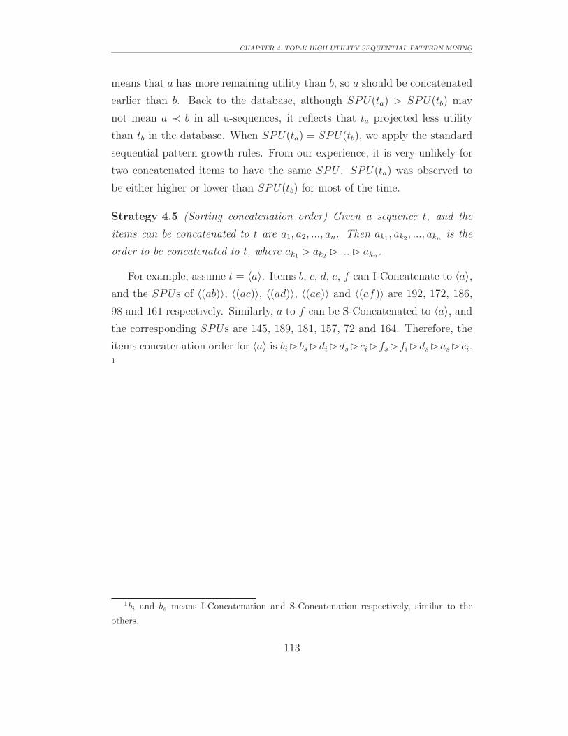
CHAPTER 4. TOP-K HIGH UTILITY SEQUENTIAL PATTERN MINING
means that a has more remaining utility than b, so a should be concatenated
earlier than b. Back to the database, although SPU(ta) > SPU(tb) may
not mean a ≺ b in all u-sequences, it reflects that ta projected less utility
than tb in the database. When SPU(ta) = SPU(tb), we apply the standard
sequential pattern growth rules. From our experience, it is very unlikely for
two concatenated items to have the same SPU . SPU(ta) was observed to
be either higher or lower than SPU(tb) for most of the time.
Strategy 4.5 (Sorting concatenation order) Given a sequence t, and the
items can be concatenated to t are a1, a2, ..., an. Then ak1 , ak2, ..., akn is the
order to be concatenated to t, where ak1 � ak2 � ...� akn.
For example, assume t = 〈a〉. Items b, c, d, e, f can I-Concatenate to 〈a〉,and the SPUs of 〈(ab)〉, 〈(ac)〉, 〈(ad)〉, 〈(ae)〉 and 〈(af)〉 are 192, 172, 186,
98 and 161 respectively. Similarly, a to f can be S-Concatenated to 〈a〉, andthe corresponding SPUs are 145, 189, 181, 157, 72 and 164. Therefore, the
items concatenation order for 〈a〉 is bi�bs�di�ds�ci�fs�fi�ds�as�ei.1
1bi and bs means I-Concatenation and S-Concatenation respectively, similar to the
others.
113

CHAPTER
4.TOP-K
HIG
HUTIL
ITY
SEQUENTIA
LPATTERN
MIN
ING
6
-
-
8
1
-
10
16
-
-
2
-
-
4
-
-
5
-
-
-
3
-
-
12
-
6
- 12 6 21
I1 I2 I3 I4 I5abcdef
(a) U-sequence 1
-
-
20
4
-
-
5
16
-
-
5
-
8
10
3
-
-
-
-
-
6
20
-
-
1
1
3 - - -
I1 I2 I3 I4 I5abcdef
-
-
8
-
1
6
I6
(b) U-sequence 2
18
-
16
10
-
-
5
-
-
-
6
-
-
4
-
-
10
4
-
5
-
-
4
6
4
-
6 - - -
I1 I2 I3 I4 I5abcdef
5
-
2
-
-
-
I6
(c) U-sequence 3
Figure 4.2: U-sequence matrices
114

CHAPTER 4. TOP-K HIGH UTILITY SEQUENTIAL PATTERN MINING
4.4 Experiments
Table 4.3: Approach Combinations
General Top-k only
SRU TUSList Sorting Pre-insertion
TUS Y Y Y Y
TUSNaive+ Y Y
TUSNaive+I Y Y Y
TUSNaive+S Y Y Y
USpan+ Y
TUSNaive Y
USpan (Yin et al. 2012)
In this section, we evaluate the performance of TUS on a variety of
datasets. Since there is no algorithm can solve the top-k high utility se-
quence mining, and it is not easy to upgrade the existing method such as
(Wu et al. 2012) either, we thus compare TUS with TUSNaive, which is a
baseline approach without pre-insertion, sorting and SRU as described in
Section 4.3.2 and 4.3.3 respectively. Two threshold-based approaches USpan
(Yin et al. 2012) and USpan+ are also used as baseline, as shown in Table
4.3.
We conduct intensive experiments on 2 synthetic and 4 real datasets to
compare the efficiency of TUS with TUSNaive and USpan/USpan+, in terms
of computational costs on different data sizes and data characteristics. To
make the top-k and threshold based approaches comparable, we run top-k
approaches first. After getting the utility of the k-th pattern, that is the
optimal minimum utility in Definition 4.1, we use this value as the minimum
threshold for running the threshold-based methods. The TUS algorithm is
implemented in C++ of Microsoft Visual Studio 2010. All experiments are
conducted on a virtual machine in a server with Intel Xeon CPU of 3.10GHz,
8GB memory and Windows 8 system.
115

CHAPTER 4. TOP-K HIGH UTILITY SEQUENTIAL PATTERN MINING
0 2000 4000 6000 8000 10000100
101
102
103
104
Tim
e(Se
c.)
K
TusTusNaiveUSpanUSpan+
(a) DS1
0 1000 2000 3000 4000 5000100
101
102
103
104
Tim
e(Se
c.)
K
TusTusNaiveUSpanUSpan+
(b) DS2
0 200 400 600 800 1000100
101
102
103
104
Tim
e(Se
c.)
K
TusTusNaiveUSpanUSpan+
(c) DS3
0 2000 4000 6000 8000 10000101
102
103
104
Tim
e(Se
c.)
K
TusTusNaiveUSpanUSpan+
(d) DS4
0 2000 4000 6000 8000 10000100
101
102
103
104
105
Tim
e(Se
c.)
K
TusTusNaiveUSpanUSpan+
(e) DS5
0 200 400 600 800 1000102
103
104
105
Tim
e(Se
c.)
K
TusUSpanUSpan+
(f) DS6
Figure 4.3: Execution time of TUS, TUSNaive, USpan and USpan+
116
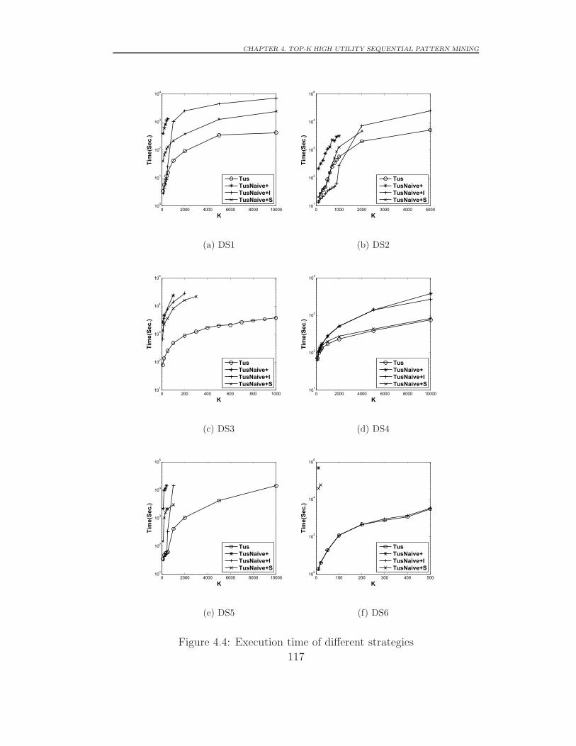
CHAPTER 4. TOP-K HIGH UTILITY SEQUENTIAL PATTERN MINING
0 2000 4000 6000 8000 10000100
101
102
103
104
Tim
e(Se
c.)
K
TusTusNaive+TusNaive+ITusNaive+S
(a) DS1
0 1000 2000 3000 4000 5000101
102
103
104
105
Tim
e(Se
c.)
K
TusTusNaive+TusNaive+ITusNaive+S
(b) DS2
0 200 400 600 800 1000101
102
103
104
105
Tim
e(Se
c.)
K
TusTusNaive+TusNaive+ITusNaive+S
(c) DS3
0 2000 4000 6000 8000 10000101
102
103
104
Tim
e(Se
c.)
K
TusTusNaive+TusNaive+ITusNaive+S
(d) DS4
0 2000 4000 6000 8000 10000101
102
103
104
105
Tim
e(Se
c.)
K
TusTusNaive+TusNaive+ITusNaive+S
(e) DS5
0 100 200 300 400 500102
103
104
105
Tim
e(Se
c.)
K
TusTusNaive+TusNaive+ITusNaive+S
(f) DS6
Figure 4.4: Execution time of different strategies
117

CHAPTER 4. TOP-K HIGH UTILITY SEQUENTIAL PATTERN MINING
We conduct experiments to evaluate the performance of TUS, in terms
of computational costs and utility changing trend, on datasets DS1 to DS6
in Table 3.4. Different strategies were compared to show their corresponding
performance on the datasets as well. Scalability tests were conducted to show
the robust of TUS approach on two synthetic datasets.
4.4.1 Execution Time Comparison With Baseline Ap-
proaches
We compared TUS with TUSNaive, USpan and USpan+ on DS1 to DS6.
The execution time of mining top-k high utility patterns by TUS are shown
in Figure 4.3. The results show that TUS is generally 10 - 1000+ times
faster than TUSNaive. For DS3 and DS4 TUSNaive cannot finish the mining
with a very small k (with k = 10 and 20) in 24+ hours. Besides, the gap
between TUS and TUSNaive increases with the increase of k. That indicates
the proposed three optimization measures, including SRU , sorting and pre-
insertion, are effective for top-k pattern mining.
The reason for USpan is faster than TUS is because the threshold is given
to USpan before mining, whereas TUS has to compute the threshold.
4.4.2 Execution Time Comparison on Different Strate-
gies
To test the efficiencies of the strategies for raising the minimum utility, we
compare the running time and the utility changing trend of the pre-insertion
and sorting. TUS, TUSNaive+, TUSNaive+I and TUSNaive+S are used in
this experiment, see Table 4.3. We incorporate SRU to all the algorithms to
compare them fairly.
The results show that TUS, TUSNaive+I and TUSNaive+S are generally
faster than TUSNaive+ from Figure 4.4, and TUS is up to 1000+ times faster
(k =10 in Figure 4.4(c)). Figure 4.5 reveals the minimum utility change trend
of the four algorithms. TUS always reaches ξ∗ shortly while TUSNaive takes
118

CHAPTER 4. TOP-K HIGH UTILITY SEQUENTIAL PATTERN MINING
0 20 40 60 80 100 120 1401000
2000
3000
4000
5000
6000
7000
8000
Min
imum
Util
ity
Time(10 Sec.)
TusTusNaive+TusNaive+ITusNaive+S
(a) DS1
0 50 100 150 200 250 300 3500
1000
2000
3000
4000
5000
6000
7000
Min
imum
Util
ity
Time(40 Sec.)
TusTusNaive+TusNaive+ITusNaive+S
(b) DS2
0 100 200 300 400 5000
500
1000
1500
2000
2500
3000
3500
4000
Min
imum
Util
ity
Time(40 Sec.)
TusTusNaive+TusNaive+ITusNaive+S
(c) DS3
0 10 20 30 40 50 600
0.5
1
1.5
2
2.5
3
3.5
4
4.5
5x 10⁴
Min
imum
Util
ity
Time(10 Sec.)
TusTusNaive+TusNaive+ITusNaive+S
(d) DS4
0 500 1000 15000
1
2
3
4
5
6x 10⁴
Min
imum
Util
ity
Time(10 Sec.)
TusTusNaive+TusNaive+ITusNaive+S
(e) DS5
0 500 1000 1500 2000 2500 30000
2
4
6
8
10
12x 104
Min
imum
Util
ity
Time(10 Sec.)
TusTusNaive+TusNaive+ITusNaive+S
(f) DS6
Figure 4.5: Changing trend comparisons
119

CHAPTER 4. TOP-K HIGH UTILITY SEQUENTIAL PATTERN MINING
much longer time to reach it. This tells that both of the strategies (sorting
and pre-insertion) effectively enhanced the performance of TUS.
Generally, TUSNaive+I is faster than TUSNaive+S when k is small. Af-
ter k exceeds a certain number, TUSNaive+S outperforms TUSNaive+I. For
example, k = 1000 in Figure 4.4(a), Figure 4.4(e) and Figure 4.4(f), k =
2000 in Figure 4.4(b), k = 20 in Figure 4.4(d). This is because TUSNaive+S
starts the mining from 0 while TUSNaive+I does not, pre-insertion directly
prunes unpromising branches than the sorting strategy. The sorting strategy
always traverses the higher estimated utility candidates first. This guaran-
tees ξ raising to ξ∗ shortly, while TUSNaive+I does not. So when k is large,
sorting is better than pre-insertion. DS3 is an exception, since the dataset
is very sparse, most of the patterns are 1-sequences. It also explains why
pre-insertion performs much better than TUSNaive+S in this dataset.
4.4.3 Scalability Test
200 300 400 500 600 700 800 900 10000
1000
2000
3000
4000
5000
6000
7000
Tim
e(se
c.)
Dataset Size(k)
Top 500Top 1000Top 1500Top 2000
(a) DS1
200 300 400 500 600 700 800 900 10000
1000
2000
3000
4000
5000
6000
Tim
e(se
c.)
Dataset Size(k)
Top 500Top 1000Top 1500Top 2000
(b) DS2
Figure 4.6: Scalability test
The scalability test is conducted to test TUS’s performance on large-scale
datasets. Sequence databases with 200K to 1000K sequences are generated
from two synthetic datasets DS1 and DS2, with the same data distribution
120

CHAPTER 4. TOP-K HIGH UTILITY SEQUENTIAL PATTERN MINING
characters we described in Table 3.4. Figure 4.6 shows the results of the
proposed TUS approach on the datasets in terms of different data sizes and
k values. By setting different k values from 500 to 2000 on both datasets,
the execution time is linear to the number of sequences.
4.5 Summary
In this chapter, we have proposed an efficient algorithm named TUS for min-
ing top-k high utility sequential patterns from utility-based sequence databas-
es. TUS guarantees there is no sequence missed during the mining process.
We have developed a new sequence boundary and a corresponding pruning
strategy for effectively filtering the unpromising candidates. Moreover, a
pre-insertion and a sorting strategy has been introduced to raise the min-
imum utility threshold. The mining performance is enhanced significantly
since both the search space and the number of candidates are effectively re-
duced by the proposed strategies. Both synthetic and real datasets have been
used to evaluate the performance of TUS, which is shown to substantially
outperform the baseline algorithms, and the performance of TUS is close
to the optimal case of the state-of-the-art utility sequential pattern mining
algorithms.
121

Chapter 5
Mining Closed High Utility
Sequential Patterns
5.1 Introduction
5.1.1 The Utility Framework
In applications like discovering frequent online shopping items, the profit of
selling associated items plays a vital role for optimizing marketing and recom-
mendation strategies. Hence, the concept utility is introduced into sequential
pattern mining to select sequences of high business value and impact. This
leads to a recent emerging area, i.e. high utility sequential pattern mining
(Yin et al. 2012, Shie et al. 2011, Ahmed, Tanbeer & Jeong 2010b, Ahmed,
Tanbeer, Jeong & Lee 2010, Yun & Leggett 2006a, Shie et al. 2013), which
selects interesting sequential patterns based on minimum utility rather than
minimum support. The utility-based patterns are proven to be more infor-
mative and actionable for decision-making (Cao 2012) than those selected
by frequency. Several efforts have been made, e.g., (Zhou et al. 2007) and
(Ahmed, Tanbeer & Jeong 2010b) discover high utility sequences in web log
data; (Shie et al. 2012) investigates high utility sequential patterns in the
mobile commerce environments; in (Yin et al. 2012), a systematic frame-
123

CHAPTER 5. MINING CLOSED HIGH UTILITY SEQUENTIAL PATTERNS
work of utility-based sequential pattern mining is provided, with an efficient
threshold-based algorithm named USpan identifying sequences satisfying a
predefined minimum utility.
5.1.2 The Limitations
Although algorithms such as UI/US (Ahmed, Tanbeer, Jeong & Lee 2010)
and USpan (Yin et al. 2012) discover the complete set of high utility se-
quences, it usually generates a large number of patterns, many of them are
redundant. Real valuable patterns which the users are interested might be
flooded in hundreds of thousands of similar patterns. Another critical issue
is that the existing methods cause dramatic running time and memory when
sequences are very long or the threshold is low, thus resulting in a huge num-
ber of patterns extracted. So far, to the best of our knowledge, no efforts
have been made to address these critical issues towards identifying highly
compact but lossless high utility sequential patterns for business purposes.
5.1.3 The Challenges of The New Framework
Is it even possible to come up with a “closed” representation of the tradi-
tional high utility sequential patterns which is compact as well as lossless?
Due to the fundamental difference, incorporating the traditional closure con-
cept into high utility sequential pattern mining makes the outcome patterns
irreversible lossy and no longer recoverable, which will be reasoned in the fol-
lowing sections. Therefore, it is exceedingly challenging for us to address the
above issues by designing a novel representation for high utility sequential
patterns.
In the frequency/support framework, closed pattern mining (Lucchese
et al. 2006, Pasquier et al. 1999, Wang et al. 2003, Zaki & Hsiao 2005, Luc-
chese et al. 2007) and closed sequential pattern mining has been extensively
studied (Tzvetkov et al. 2005, Yan et al. 2003, Cong et al. 2005, Huang,
Chang, Tung & Ho 2006, Wang & Han 2004). A pattern is closed if it has no
124

CHAPTER 5. MINING CLOSED HIGH UTILITY SEQUENTIAL PATTERNS
super-patterns of the same support. Closed patterns can be considered as a
compact and lossless representation of all patterns, and are widely recognized
better than non-closed because: 1) the number of patterns is usually much
less, and 2) the later can be completely recovered from the former, in other
words, lossless. The frequent closed representation is naturally lossless since
all the subsets of a closed pattern are exactly the same frequent as that pat-
tern. However, such a property does not hold in the utility framework since a
pattern’s utility may not be the same as its superpattern’s even if they have
the same support (Yin et al. 2012). We will illustrate with examples that
the approaches of mining closed sequential patterns such as CloSpan(Yan
et al. 2003) can not be applied in the utility framework in the remainder
of the chapter. In (Wu et al. 2011), the authors proposed a concise and
lossless representation named “closed+ high utility itemsets”, and provid-
ed CHUD and DAHU to discover and recover closed high utility itemsets.
But CHUD cannot be applied to the high utility sequential pattern mining.
This is caused by the intrinsic difference between itemset and sequence. The
itemset mining (either frequency or utility based) assumes pattern A has the
same support as its super pattern B, then 1) transactions containing A and
B are exactly the same, and 2) in each transaction, the items in A must also
be in B. With 1), frequent closed patterns can be easily recovered to the
complete set. With 1) and 2), both patterns and utilities can be easily main-
tained and recovered. However, a sequence may match its supersequence in
multiple ways, and multiple utilities of a single sequence may be obtained.
So, suppose A is a supersequence of B and they have the same support, then
A’s utility might be higher than B’s in the utility sequence scenario, which
never holds in (Wu et al. 2011).
5.1.4 Research Contributions
Designing a lossless representation of high utility sequential pattern is a chal-
lenging task. It is even harder to extract such patterns. The contributions
include:
125

CHAPTER 5. MINING CLOSED HIGH UTILITY SEQUENTIAL PATTERNS
• We propose a concise and lossless framework for discovering US-closed
high utility sequential patterns. Based on a series of novel definitions
such as maximum item utility and distinct occurrence which have n-
ever been used in the state-of-art research, we theoretically prove the
proposed representation/framework is compact and lossless.
• An efficient algorithm CloUSpan is proposed to discover US-closed high
utility sequences. We systematically analyzed the extraction of US-
closed patterns on-the-fly, including the three types of newly discov-
ered patterns that can cover existing patterns, be covered by existing
patterns or neither.
• Two effective strategies are used to enhance the performance of CloUS-
pan. Based on the framework, we proposed early pruning strategy and
skipping scanning strategy to avoid unnecessary searches. Both of the
strategies are not only theoretically proved, but also explained with
detail example.
The rest of this chapter is organized as follows. In Section 5.2, we present
our proposed US-closed framework and propose CloUSpan with two strate-
gies. Experiments are shown in Section 5.3 and the conclusions is in Section
5.4.
5.2 US-closed High Utility Sequential Pat-
tern Mining
In this section, we present a concise and lossless representation of high utility
sequential patterns. Some readers might be curious why not directly put the
close constraint on high utility sequential patterns, since this is the solution
used in (Wu et al. 2011). However, it cannot be applied due to the funda-
mental difference between sequential pattern mining and itemset mining. We
discuss this in detail first.
126

CHAPTER 5. MINING CLOSED HIGH UTILITY SEQUENTIAL PATTERNS
SID TID Transactions TU SU
1 1 (a,6)(d,8)(e,1) 15
112
1 2 (b,10)(c,16)(f,2) 28
1 3 (a,12)(d,4) 16
1 4 (a,6)(b,5)(f,3) 14
1 5 (a,21)(d,12)(f,6) 39
2 1 (c,20)(d,4) 24
117
2 2 (a,3)(b,5)(c,16)(f,5) 29
2 3 (c,8)(d,10)(e,3) 21
2 4 (f,6) 6
2 5 (b,20)(e,1)(f,1) 22
2 6 (a,6)(d,8)(f,1) 15
3 1 (a,18)(b,16)(d,10) 44
105
3 2 (a,6)(b,5)(f,6) 17
3 3 (d,4) 4
3 4 (b,10)(c,4)(e,5) 19
3 5 (c,4)(e,4)(f,6) 14
3 6 (b,5)(d,2) 7
Table 5.1: U-sequence Database
Definition 5.1 (High utility sequence set) Given a utility sequence database
S and a minimum utility ξ, the high utility sequential pattern set is denoted
and defined as L(S, ξ) = {t|∃s ∈ S, s.t. s � t∧ umax(t) ≥ ξ}, or abbreviated
as L.
Definition 5.2 (Closed high utility sequence set) Given a u-sequence database
S and a minimum utility ξ, a US-closed high utility sequential pattern set
is denoted as C(S, ξ) (or abbreviated as C), where C(S, ξ) ⊆ L(S, ξ), and
∀tc ∈ C(S, ξ), �t ∈ C(S, ξ), such that |S(tc)| = |S(t)| and tc ⊆ t.
Obviously, Definition 5.2 puts a closure constraint on the results from
Definition 5.1. It can be interpreted as below: we first mine on S to obtain
127

CHAPTER 5. MINING CLOSED HIGH UTILITY SEQUENTIAL PATTERNS
L, then for each pattern in L, find its supersequence. If there exists one
with the same support, then the pattern can be removed from L, and the
remaining patterns in L is exactly C.The above method works for high utility itemset mining (Wu et al. 2011),
because if a pattern is contained by a transaction, there is only one way to
match the items. For example, u-itemset [(a, 3)(b, 5)(c, 16)(f, 5)] contains
(ac), that is [(a, 3)(c, 16)] ∼ (ac). However, in our problem, there is not such
a nice feature. In fact our problem is far more difficult with the following
property.
Property 5.1 Suppose t′ ⊂ t and |S(t′)| = |S(t)|. If t is extracted from
a transaction/itemset database, then u(t) > u(t′); if t is extracted from a
sequence database, then u(t) may be bigger, smaller or equal to u(t′).
Readers can refer to (Wu et al. 2011) for the former part about item-
set. For the sequence property, we illustrate it with an example in Table
5.1. 〈(cde)〉 and 〈(cd)〉 are two sequences contained by s2, so |S(〈(cde)〉)| =|S(〈(cd)〉)| = 1, 〈(cd)〉 ⊆ 〈(cde)〉, which means both 〈(cd)〉 can be ab-
sorbed by 〈(cde)〉 according to (Yan et al. 2003). However, umax(〈(cde)〉) =u(〈(cde)3〉) = 21 but umax(〈(cd)〉) = u(〈(cd)1〉) = 24, so umax(〈(cd)〉) >
umax(〈(cde)〉). The reason is as follows. u(〈(cd)〉) = {u(〈(c d)1〉), u(〈(cd)3〉)} =
{24, 18}, if 〈(cde)〉 absorbs 〈(cd)〉, then u(〈(cd)1〉) is lost forever, which means
〈(cde)〉 can never recover 〈(cd)〉’s utility. Therefore, in the utility sequence
framework, L to C is irreversible.
This is fatal for the methods and techniques used in support/frequency-
based closed sequence mining algorithms such as CloSpan (Yan et al. 2003)
to be applied in the utility framework. CloSpan, as an example, removes
all the short sequences whoever contained by a supersequence with the same
support. Because the short sequential patterns and their supports can be
easily recovered. For example, in Table 5.1, sequential pattern 〈a〉 should be
removed because 〈a〉 ⊆ 〈ab〉, and the support of 〈ab〉 is also 3. Thus, 〈a〉 canbe recovered from 〈ab〉.
128
CHAPTER 5. MINING CLOSED HIGH UTILITY SEQUENTIAL PATTERNS
With Property 5.1, the closed patterns cannot be recovered, which means,
lossy. We have to redesign a lossless representation and completely re-define
the “closed” high utility sequential patterns. Below, we discuss the US-closed
high utility patterns in detail.
5.2.1 US-closed High Utility Sequences
Definition 5.3 (Maximum item utility) Given a sequence t and a u-sequence
s, let 〈i1〉, 〈i2〉, ...〈in〉 where ik ∈ I, 1 ≤ k ≤ n are all the 1-sequences belonging
to t. Assume that 〈(i1, u1)〉, 〈(i1, u2)〉...〈(i1, um1)〉 be all the u-items in s that
match 〈i1〉, and u1 > u2 > ... > um1. Suppose the number of i1 in t is l1, the
maximum item utility of i1 in t is denoted and defined as
miu(i1, t, s) =
l1∑
i=1
ui (5.2.1)
The maximum item utility of t in s and S are denoted and defined as
miu(t, s) =n∑
i=1
miu(ii, t, s) (5.2.2)
miu(t) =∑
s∈Smiu(t, s) (5.2.3)
Intuitively, the maximum item utility relaxes the order constraint on item-
s, and is the sum of the highest items’ utilities. As an example shown in
Figure 5.1, first, we illustrate the u-sequence s1 as the matrix display on
the top on the left. I1 to I5 in its header line represent the u-itemsets of
TID = 1 to 5, the numbers in the cells are the utilities of the corresponding
item, and “-” means there is nothing in that position in s1. In our imple-
mentation, we construct the linked-sorted-list structure at right hand side
where the utilities in each row are descending-sorted. When a new sequence
such as t = 〈(ad)a〉 arrives, the miu value is calculated as the following way.
miu(a, 〈(ad)a〉, s1) = (21 + 12) = 33, miu(d, 〈(ad)a〉, s1) = 12, miu(〈(ad)a〉, s1) = (33 + 12) = 45 and miu(〈(ad)a〉) = (45 + 34) = 79.
Obviously, for any sequence t, miu(t) ≥ umax(t) holds.
129

CHAPTER 5. MINING CLOSED HIGH UTILITY SEQUENTIAL PATTERNS
6--81-
1016--2
--4--
5---3
--
12-6
- 12 6 21I1 I2 I3 I4 I5
abcdef
2110161216
5
8
3
4
2
12 6 6abcdef
sequence t = <(ad)a>
the items in t: a d
In item level: miu(a, <(ad)a>, s1) = 21 + 12 = 33, miu(d, <(ad)a>, s1) = 12
In sequence level: miu(<(ad)a>, s1) = 33 + 12 = 45, miu(<(ad)a>, s2) = 34
In database level: miu(<(ad)a>) = 45 + 34 = 79
Sorted listu-sequence s1
Figure 5.1: An example of calculating miu
Definition 5.4 (Distinct Occurrence) Given two sequences (or u-sequences)
t1 and t2, we say t2 uniquely contains t1 iff there is only one t′2 ⊆ t2 such
that t1 = t′2, denoted as t1 � t2. Similarly, for a sequence t and a u-sequence
s, s uniquely contains t, denoted as t � s, iff there is only one s′ and s′ ⊆ s
such that s′ ∼ t.
For example, 〈(ad)〉 � 〈(ad)a〉 and 〈aa〉 � 〈(ad)a〉, but 〈a〉 � 〈(ad)a〉,because a appears twice in 〈(ad)a〉. Please be aware that the “�” is not
transitive. More formally, it is possible that t1 � t2 and t2 � t3, t1 � t3.
For example, 〈(ad)〉 � 〈(ad)a〉 and 〈a〉 � 〈(ad)〉. And also notice that the
condition of t � s (t is a sequence and s is a u-sequence) does not imply
miu(t) = umax(t). Because for each item in t, there might be multiple same
130

CHAPTER 5. MINING CLOSED HIGH UTILITY SEQUENTIAL PATTERNS
u-items with different utilities in s.
Definition 5.5 (Vertical Utility Array) Given a sequence t = 〈(p11p12...p1k1)(p21p22...p2k2)...(pl1pl2...plkl)〉, where for 1 ≤ i ≤ l, 1 ≤ j ≤ ki, pij is an item
and (pi1pi2...piki) ⊆ I is an itemset. Given two u-sequences s′ and s, where
s′ ∼ t, s′ ⊆ s and s′ = 〈[(p11, u11)(p12, u12)...(p1k1 , u1k1)][(p21, u21)(p22, u22)...
(p2k2 , u2k2)]...[(pl1, ul1)(pl2, ul2)...(plkl, ulkl)]〉. Suppose �s′′ ⊆ s where s′′ ∼ t
and u(s′′) > u(s′).The vertical utility array of t in u-sequence s is denoted and
defined as Us(t, s) = 〈(u11u12...u1k1)(u21u22... u2k2)...(ul1ul2...ulkl)〉, which is
exactly the same as the utilities of the u-items in s′. The uij in Us(t, s) is de-
noted and defined as U ijs (t, s) = uij. Us(t) denotes the vertical utility array of
t in S, which is defined as Us(t) = 〈(u′11u
′12...u
′1k1
)(u′21u
′22...u
′2k2
)...(u′l1u
′l2...u
′lkl)〉.
u′ij in Us(t) is defined as
u′ij =
∑
s0∈S(t)U ijs (t, s0) (5.2.4)
<(a d) a>
12 4 21
18 10 6
sequence: t =
Us(t, s1) =
Us(t, s3) =
30 14 27Us(t) =
<[(a,12) (d,4)] (a,21)>s’1 =
<[(a,18) (d,10)] (a,6)>s’3 =
Figure 5.2: The vertical utility array
The vertical utility array Us is a vertical utility representation of se-
quences. For example, in Figure 5.2, Us(〈(ad)a)〉) = 〈((12+18), (4+10)); (21+
6)〉 = 〈(30, 14); 27〉. The three numbers 30, 14 and 27 represent the verti-
cal utilities of a1, d1 and a2 in 〈(ad)a)〉 respectively. Then, we can have the
following two lemmas.
Lemma 5.2 The utility of a sequence can be calculated from its vertical u-
tility array.
umax(t) =∑
Us(t) (5.2.5)
131

CHAPTER 5. MINING CLOSED HIGH UTILITY SEQUENTIAL PATTERNS
Proof Assume sequence s1, s2, ..., sn contain t and for s′k ⊆ sk(1 ≤ k ≤ n),
�s′′k ⊆ sk such that u(s
′′k) ≥ u(s′k). Suppose the ith item’s utility in s′k is uik,
and the number of items in t is l. The utility of t is
umax(t) =n∑
k=1
l∑
i=1
uik
=
l∑
i=1
n∑
k=1
uik
According to the Definition 5.5,
umax(t) =l∑
i=1
U is(t)
Where U is(t) is the vertical sum utility of the ith item in t,
umax(t) =∑
Us(t)
Until now, we have prove that the utility of t can be represented by the
vertical utility array.
Lemma 5.3 Given a sequence t, let t′ � t. Suppose the Us(t) is known, then
Us(t′) ⊆ Us(t).
Proof Suppose the length of t and t′ are n and n′ respectively. Since t′ � t,
which means t′ is uniquely contained in t, each item in t′ can be mapped to t.
Suppose the i1, i2, ..., i′n are the items’ indexes in t, which is t(i1, i2, ..., i
′n) = t′.
Therefore, t′’s vertical utility array is Us(t′) = 〈U i1
s (t), U i2s (t), ..., U
i′ns (t)〉. The
lemma holds.
Theorem 5.4 Given a database S and a sequence t. If
1)umax(t) =∑
s∈Smiu(t, s), and
2)∀t′ ⊆ t, |S(t′)| = |S(t)|
and t is closed, then ∀t′ � t, Us(t′) can be calculated from Us(t) and
umax(t′) =
∑Us(t
′) (5.2.6)
132

CHAPTER 5. MINING CLOSED HIGH UTILITY SEQUENTIAL PATTERNS
Proof Based on condition 2) ∀t′ ⊆ t, |S(t′) = S(t)|, we have S(t′) = S(t).Since umax(t) =
∑s∈S miu(t, s), then ∀s ∈ S and s � t, based on Lemma 5.2,
the utility of t in s is umax(t, s) = miu(t, s). In other words, the items in t
matches the highest utility sub-u-sequence in the sub-u-sequences that match
s. Then given t′ � t, according to Lemma 5.3, Us(t′) ⊆ Us(t). Therefore,
umax(t′) =
∑s∈S miu(t′, s) =
∑Us(t
′).
The above theorem shows if a sequence satisfies the given conditions, then
it is able to recover any of its subsequences that are uniquely contained by
itself without losing information. It guarantees that our proposed represen-
tation has the capability to compress and recover sequences concisely. Please
be aware of that umax(t, s) = miu(t, s) =∑n
i=1miu( ti, t, s) doesn’t imply
t � s, since there might be multiple s′ ⊆ s, s′ ∼ t and u(s′) = umax(t, s).
Example 5.5 Let t0 = 〈cf〉, and Us(t0) = 〈((16 + 20 + 4); (6 + 6 + 6))〉 =〈(40; 18)〉, since umax(t0) = 22 + 26 + 10 = 58 which is equal to miu(t0),
and |S(t0)| = |S(〈c〉)| = |S(〈f〉)| = 3. t0 satisfies the conditions of Theorem
5.4, therefore 〈c〉 and 〈f〉 can be absorbed by t0. To recover 〈c〉 and 〈f〉 fromt0, because both of them are uniquely contained by 〈cf〉, their vertical utility
arrays can be calculated from Us(t0), which are Us(〈c〉) = 〈40〉 and Us(〈f〉) =〈18〉 respectively. Furthermore, according to Lemma 5.2, umax(〈c〉) = 40 and
umax(〈c〉) = 18.
Definition 5.6 (US-closure) Sequence t is called US-closure to another se-
quence t′, denoted as t ⇒ t′ iff 1)t′ � t, 2)umax(t) =∑
s∈S miu(t, s),
3)|S(t′)| = |S(t)|, and 4) Us(t) is known.
By now we have presented the proposed US-closure representation as
Definition 5.6 is losslessly recoverable. The reason is the utility of t′ can be
calculated by the vertical utility array Us(t′) of t′ according to Lemma 5.2,
and Us(t′) can be recovered from Us(t) by Theorem 5.4, as stated above.
Basically, t ⇒ t′ means that t′, including Us(t′) and umax(t), can be correctly
recovered from t. We can now put the US-closure constraint on the tradi-
133

CHAPTER 5. MINING CLOSED HIGH UTILITY SEQUENTIAL PATTERNS
tional high utility sequential patterns to present the US-closed high utility
sequences as the definition below.
Definition 5.7 (US-closed high utility sequence) Given a u-sequence database
S, a minimum utility ξ, the US-closed high utility sequential pattern set is
denoted as U(S, ξ), where U(S, ξ) ⊆ L(S, ξ), and ∀tu ∈ U(S, ξ), �t ⊆ tu and
t ∈ U(S, ξ), s.t. t ⇒ tu.
The US-Closed high utility sequential pattern set can be losslessly recov-
ered to the complete set of non-US-closed ones. The novel representation
delivers a compact result with less redundancy. It is essential to develop
approaches, namely US-closed high utility sequential pattern mining algo-
rithm, to extract U from S. In the next section, we discuss how to extract
U efficiently in detail.
5.2.2 CloUSpan
In the previous section, we proved the US-closed high utility sequential pat-
tern can be losslessly recovered. In the next two sections, we discuss how to
efficiently extract high utility sequential patterns and how to recover them.
We start from the algorithm CloUSpan to extract US-closed high utility se-
quences.
Suppose t is a k-sequence, we call the operation of appending a new item
α to the end of t to form (k+1)-sequence concatenation, denoted as t � α.
If the size of t does not change, it is I-Concatenation, denoted as t �i α.Otherwise, if the size increases by one, we call it S-Concatenation, denoted
as t �s α. Mining L is a process of recursively constructing candidates and
comparing the minimum utility threshold. It usually includes a series of
I-Concatenation and S-Concatenation processes like 〈〉 → 〈a〉 → 〈(ab)〉 →〈(ab)c〉 → 〈(ab)(cd)〉 → ... When reaching the leaf node, it backtracks some
high level nodes and repeats the process again and again until no more nodes
to travel. Here, let t0 = t � t′, we call t0 the offspring of t. Specifically, if the
length of t′ equals to 1, in other words, an item, then we call t0 the child of
134

CHAPTER 5. MINING CLOSED HIGH UTILITY SEQUENTIAL PATTERNS
t. For example, 〈(ab)〉 and 〈ab〉 are children as well as offsprings of 〈a〉, but〈(ab)c〉 and 〈abc〉 can be only said 〈a〉’s offsprings.
Now we have proved that some high utility sequential patterns can recov-
er others losslessly, but it cannot be directly used to skip constructing the
patterns that can be absorbed. Because it is impossible to identify the final
US-closed patterns in a mining process. To tackle this issue, we use a tempo-
rary list to store the US-closed pattern found so far. The patterns in the list,
however, are only temporary US-closed to the others. Suppose a previously
discovered US-closed pattern set U ′ is maintained, we can generally classify
a newly discovered pattern t into three types.
1 ∃t′ ∈ U ′, such that t′ ⇒ t,
2 ∃t′ ∈ U ′, such that t ⇒ t′
3 �t′ ∈ U ′, such that t ⇒ t′ or t′ ⇒ t.
For Type 1, we simply discard t since it can be absorbed by some discov-
ered pattern in U ′; A Type 2 pattern exists when some patterns in current
U ′ can be absorbed, which should be removed from U ′ and have t inserted;
In Type 3, t is also inserted since it couldn’t be represented by any pattern
in U . Essentially, we can use Types 1 to control computational costs. Oper-
ations on Type 2 guarantee the correct results without redundant patterns
and controls the size of U . Newly found patterns in Type 3 whoever matches
ξ, we simply leave them in a temporary list. Next, we discuss how to avoid
invalid searches and checking from Types 1.
Early Pruning Strategy
Now we discuss a situation in Type 1 where we can utilize our strategy to
prune unnecessary searches.
Theorem 5.6 Let t ⇒ t′ be two sequences. ∀t0, if (t′ � t0) � t and |S(t′ �t0)| = |S(t)|, then t ⇒ (t′ � t0).
135

CHAPTER 5. MINING CLOSED HIGH UTILITY SEQUENTIAL PATTERNS
Proof According to Definition 5.6, t ⇒ t′ means t’s utility can be calculated
via umax(t) =∑
s∈S miu(t, s). ∀t1 � t, if |S(t1)| = |S(t)|, then t1’s vertical
utility array Us(t1) can be recovered (Lemma 5.2). t1’s utility is therefore
can be calculated by summing its Us(t1), that is umax(t1) =∑
Us(t1).
Basically, the theorem is a direct consequence of the Definition 5.6 and
Theorem 5.4. It says that if a sequential pattern t can absorb a sub pattern
t0, it can also absorb some super pattern of t0 whose length is less than
t. The rule can dismiss some redundant patterns. However, in the mining
process, t can never be found before t0 and the others. We further propose
the corollary below to make the theorem prunable.
Corollary 5.7 (Early pruning) Suppose t ⇒ t′ and t′ � t0 = t, if there are
no duplicated items1 in t0, then ∀t1 ⊆ t0, t ⇒ (t′ � t1).
Proof t ⇒ t′ means t′ � t. There is only one way to match every item
in t′ to t. Since there are no duplicated items after t0, so for any t1 ⊆ t0,
(t′ � t1) � t. Therefore, t ⇒ (t′ � t1).
In order to help understanding the strategy, we use a simple example to
illustrate. Suppose the current candidate is 〈a(ab)〉 and a US-closed pattern
〈a(ab)cd(ae)〉 is in the temporary list. Obviously, 〈a(ab)cd(ae)〉 ⇒ 〈a(ab)〉,and there is no duplicated items in 〈cd(ae)〉. Without the strategy, it will
continue constructing useless candidates such as 〈a(ab)a〉 and 〈a(abd)〉. Andit will recursively go deep into each successor of those useless candidates
until all are traversed. However, with Corollary 5.7, we can simply avoid
concatenating and testing unnecessary candidates since they can be absorbed
by a longer pattern. If a newly candidate is constructed and found matching
the conditions, it can be directly pruned.
1Here, “no duplicated items” means that there is no item appears more than once in
t0. For example, 〈(ad)a〉 has a duplicated item a who has occurred twice, and 〈cf〉 has noduplicated items.
136

CHAPTER 5. MINING CLOSED HIGH UTILITY SEQUENTIAL PATTERNS
Skipping Scanning Strategy
Early pruning strategy greatly reduces the search space. However, not many
candidates could match the strict condition for pruning. Now we introduce
another strategy to avoid invalid scanning for new candidates in the imme-
diate next level. First, let us begin with the following definitions.
Definition 5.8 (Terminal point and pivot) Suppose that all the (u-)items in
the (u-)sequences are listed alphabetically. Let s = 〈l1l2...ln〉 be a u-sequence,
t = 〈t1t2...tm〉 be a sequence and s � t, assume sa = 〈la1la2 ...lam〉, where
lam = [(ip1, qp1)(ip2 , qp2)... (ipm′ , qpm′ )], sa ⊆ s and sa ∼ t, (ipm′ , qpm′ ) is called
the Terminal point of t in s. Additionally, (ipm′ , qpm′ ) is called pivot iff there
is no sb = 〈lb1lb2 ...lbm〉 where sb ⊆ s and sb ∼ t such that bm < am.
For example, the terminal point of 〈(ad)a〉 in s1 are a3, a4 and a5, where
the pivot is a3. For 〈d(bf)〉 in s1, the terminal points are f2 and f4.
Definition 5.9 (Remaining utility) Given a sequence t, a u-sequence s and
a u-sequence database S, the remaining utility of t in s and S are denoted
and defined as:
uru(t, s) =∑
i′∈s∧i≺i′u(i′) (5.2.7)
uru(t) =∑
s′∈Suru(t, s
′) (5.2.8)
where i is the pivot of t in s.
Basically, the remaining utility of a sequence means the sum of the util-
ities after the pivot. For example, the remaining utility of 〈(ad)a〉 in s1 is
uru(〈(ad)a〉, s1) = 4 + (6 + 5 + 3) + (21 + 12 + 6) = 4 + 14 + 39 = 57, and
uru(〈(ad)a〉) = uru(〈(ad)a〉, s1) + uru(〈(ad)a〉, s3) = 57 + 55 = 112. Then we
present the following definition and theorem.
Definition 5.10 (Cut containment) Let t′ ⊆ t be two sequences, if umax(t) =
miu(t), umax(t′) = miu(t′) and uru(t) = uru(t
′), we called it cut containment,
denoted as t′ ⊆p t.
137

CHAPTER 5. MINING CLOSED HIGH UTILITY SEQUENTIAL PATTERNS
Theorem 5.8 Given t′ ⊆p t, let t0 be a sequence and umax(t � t0) > 0,
umax(t �s t0) > umax(t′ �s t0).
Proof From the definition of t′ ⊆p t, we have t′ ⊆ t, umax(t) = miu(t),
umax(t′) = miu(t′) and uru(t) = uru(t
′). Since t′ ⊆ t and uru(t) = uru(t′),
then S(t′) = S(t). It also means the pivots of t and t′ are at the exactly same
point in all the u-sequences. With umax(t) = miu(t) and umax(t′) = miu(t′),
umax(t) > umax(t′). Therefore, any sequence t0 concatenates to t and t′, the
utility of the former is always higher than the latter. The theorem holds.
Corollary 5.9 (Skip scanning) Given t′ ⊆p t, let t0 be a sequence and
umax(t � t0) > 0, then the offspring of t′ whose utilities are no less than
ξ is a subset of that of t.
Proof From Theorem 5.8, we have umax(t �s t0) > umax(t′ �s t0) for any t0.
So it’s easy to understand that if umax(t′ �s t0) > ξ, then umax(t �s t0) >
umax(t′ �s t0) > ξ. However, if umax(t �s t0) > ξ, umax(t
′ �s t0) cannot be
judged larger or smaller than ξ.
Corollary 5.9 ensures to skip the scanning of children of patterns which
cannot be pruned by Corollary 5.7 but still satisfy t′ ⊆p t. Without the strat-
egy, the projected database has to be scanned every time a new candidate
is generated, which is very time consuming. Now we introduce the proposed
CloUSpan algorithm as follows.
CloUSpan
With Corollary 5.7 and 5.9 (the two strategies), we now present CloUSpan
as below.
The pseudo code of CloUSpan is provided in Algorithm 5.1. The al-
gorithm takes a u-sequence database S and a minimum utility ξ as input
parameters, and output the complete set of US-closed high utility sequential
patterns U(S, ξ). Lines 1-2 and Lines 3-6 correspond to Corollary 5.7 and 5.9
respectively. Line 4 means that the items to be concatenated are required
138
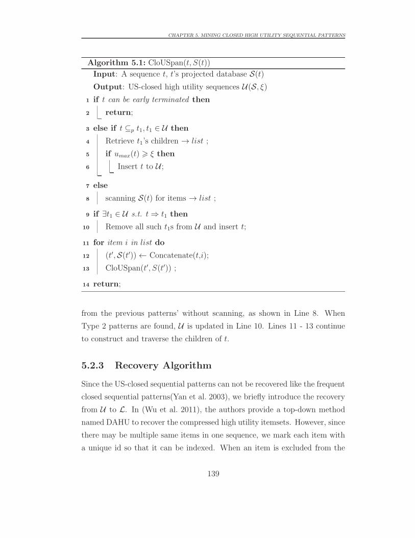
CHAPTER 5. MINING CLOSED HIGH UTILITY SEQUENTIAL PATTERNS
Algorithm 5.1: CloUSpan(t, S(t))
Input: A sequence t, t’s projected database S(t)Output: US-closed high utility sequences U(S, ξ)
1 if t can be early terminated then
2 return;
3 else if t ⊆p t1, t1 ∈ U then
4 Retrieve t1’s children → list ;
5 if umax(t) � ξ then
6 Insert t to U ;
7 else
8 scanning S(t) for items → list ;
9 if ∃t1 ∈ U s.t. t ⇒ t1 then
10 Remove all such t1s from U and insert t;
11 for item i in list do
12 (t′,S(t′)) ← Concatenate(t,i);
13 CloUSpan(t′, S(t′)) ;
14 return;
from the previous patterns’ without scanning, as shown in Line 8. When
Type 2 patterns are found, U is updated in Line 10. Lines 11 - 13 continue
to construct and traverse the children of t.
5.2.3 Recovery Algorithm
Since the US-closed sequential patterns can not be recovered like the frequent
closed sequential patterns(Yan et al. 2003), we briefly introduce the recovery
from U to L. In (Wu et al. 2011), the authors provide a top-down method
named DAHU to recover the compressed high utility itemsets. However, since
there may be multiple same items in one sequence, we mark each item with
a unique id so that it can be indexed. When an item is excluded from the
139

CHAPTER 5. MINING CLOSED HIGH UTILITY SEQUENTIAL PATTERNS
sequence, its corresponding utility unit is removed from Us. We implement
the recovery on top of CloUSpan to conduct experiments as shown in the
next section.
5.3 Experiments
In this section, we evaluate the performance of CloUSpan on a variety of
datasetss. We compare CloUSpan with USpan (Yin et al. 2012), which is
the baseline algorithm for mining high utility sequential patterns. Intensive
experiments on two synthetic and four real datasets are conducted to com-
pare the efficiency of the two algorithms, in terms of computational costs of
different data sizes and data characteristics. Both CloUSpan and USpan are
implemented in C++ of Microsoft Visual Studio 2010. All experiments are
conducted on a virtual machine in a server with Intel Xeon CPU of 3.10GHz,
16GB memory and Windows 8 system.
5.3.1 Performance
In this part, we compare the performance of the proposed CloUSpan algo-
rithm with USpan on all the six datasets. Notice that CloUSpan (referred
as “CloUSpan” in Figure 5.3) only extracts all the US-closed sequential pat-
terns, we also implement the decompression algorithm on top of CloUSpan
(referred as “CloUSpan + R”) to recover the complete set of high utility
sequences. The decompression algorithm recovers from the US-closed se-
quential patterns, so it can only be run after CloUSpan is finished. On the
other hand, we run USpan(referred as “USpan”) on the same datasets to
extract the high utility sequential patterns. According to our experiments,
the results from “CloUSpan + R” and “USpan” are exactly the same. It
reveals that the proposed US-closed representation is lossless.
As seen from the figures, both CloUSpan and CloUSpan+R outperform
USpan in terms of the running time. In Figure 5.3(a) (ξ = 0.0754%) and
Figure 5.3(c) (ξ = 0.1732%), CloUSpan is almost 1000 times faster than
140

CHAPTER 5. MINING CLOSED HIGH UTILITY SEQUENTIAL PATTERNS
0.075 0.08 0.085 0.09100
101
102
103
104
Tim
e(Se
c.)
Threshold (%)
USpanCloUSpanCloUSpan + R
(a) DS1
0.075 0.08 0.085 0.09 0.095 0.1 0.105101
102
103
Tim
e(Se
c.)
Threshold (%)
USpanCloUSpanCloUSpan + R
(b) DS2
0.1731 0.1732 0.1733 0.1734 0.1735 0.1736 0.1737 0.1738 0.1739100
101
102
103
104
Tim
e(Se
c.)
Threshold (%)
USpanCloUSpanCloUSpan + R
(c) DS3
0 0.2 0.4 0.6 0.8 1101
102
103
104
Tim
e(Se
c.)
Threshold (%)
USpanCloUSpanCloUSpan + R
(d) DS4
0.0572 0.0574 0.0576 0.0578 0.058 0.0582 0.0584102
103
104
Tim
e(Se
c.)
Threshold (%)
USpanCloUSpanCloUSpan + R
(e) DS5
3 4 5 6 7 8 9 10
x 10-3
103
104
105
Tim
e(Se
c.)
Threshold (%)
USpanCloUSpanCloUSpan + R
(f) DS6
Figure 5.3: Performance comparisons
141

CHAPTER 5. MINING CLOSED HIGH UTILITY SEQUENTIAL PATTERNS
USpan. It shows that the proposed strategies are effective for pruning the
searching space. The density of DS4 is the highest. Since there are too many
duplicated items in one sequence, there is little chance for the patterns to be
“absorbed” by any super-pattern (It is against the unique containment rule
“�” of Theorem 5.4). It performs only a little faster because some scanning
processes are skipped. DS6, however, is a very sparse dataset. When the
threshold is high, the patterns have no closure relationship to each other, for
which the algorithms only show a little gap.
5.3.2 Memory Usage
We also compared the proposed CloUSpan with USpan algorithm in terms
of the memory usage, as shown in Figure 5.4. Since the decompression al-
gorithm runs on the result of CloUSpan after CloUSpan is done, plus the
memory consumption is tiny (always less than 20MB), so we skip comparing
it in this part. The X axis in Figure 5.4 means ξ, and the Y axis means the
memory usage measured in Mega Bytes of CloUSpan (marked in dot) and
USpan (in circle).
As shown by these figures, CloUSpan costs less memory consumption,
and saves up to 10+ times space compared with USpan (ξ = 0.0754% in
Figure 5.4(a) and ξ = 0.1732% Figure 5.4(c)). The evaluation shows that
our proposed algorithm with the strategies can very effectively control the
memory usage on either very large datasets or very low minimum utility.
Corollary 5.7 and Corollary 5.9 are the keys to explain the results. In
detail, Corollary 5.7 terminates invalid concatenation processes from going
too deep, and the space of storing those unnecessary projected databases
are saved. The scanning for concatenation items process is also very space
costly. It needs to store every promising item and its related information in
the memory dynamically. Corollary 5.9 skips the scanning process by directly
retrieving the items from the previous mined patterns, and the space is saved.
142

CHAPTER 5. MINING CLOSED HIGH UTILITY SEQUENTIAL PATTERNS
0.075 0.08 0.085 0.09101
102
103
104
Mem
ory
Usa
ge(M
B)
Threshold (%)
USpanCloUSpan
(a) DS1
0.075 0.08 0.085 0.09 0.095 0.1 0.105102
103
104
Mem
ory
Usa
ge(M
B)
Threshold (%)
USpanCloUSpan
(b) DS2
0.1731 0.1732 0.1733 0.1734 0.1735 0.1736 0.1737 0.1738 0.1739101
102
103
104
Mem
ory
Usa
ge(M
B)
Threshold (%)
USpanCloUSpan
(c) DS3
0 0.2 0.4 0.6 0.8 1
103.5
103.6
103.7
103.8
Mem
ory
Usa
ge(M
B)
Threshold (%)
USpanCloUSpan
(d) DS4
0.0572 0.0574 0.0576 0.0578 0.058 0.0582 0.0584
102.7
102.8
102.9
Mem
ory
Usa
ge(M
B)
Threshold (%)
USpanCloUSpan
(e) DS5
3 4 5 6 7 8 9 10
x 10-3
103.5
103.6
Mem
ory
Usa
ge(M
B)
Threshold (%)
USpanCloUSpan
(f) DS6
Figure 5.4: Memory usage comparisons
143

CHAPTER 5. MINING CLOSED HIGH UTILITY SEQUENTIAL PATTERNS
5.3.3 Number of Candidates
To further investigate the effectiveness of the proposed strategy, we compare
the number of candidates generated by CloUSpan and USpan in their mining
processes. Basically, the number of candidates is calculated by counting how
many times of line 12 in Algorithm 5.1 is being executed, since each time a
new candidate t′ is generated.
As shown in Figure 5.5, CloUSpan always generated less candidates com-
pared with USpan. It tells that Corollary 5.7 is effective, and further explains
Figure 5.3. However, sometimes both algorithms generate the same number
of candidates but the running time and memory costs are different. For exam-
ple, ξ = 0.0754% in Figure 5.5(c), all scatters in Figure 5.5(d), ξ = 0.0576%
to ξ = 0.58% in Figure 5.5(e) and ξ = 0.0036% to ξ = 0.009% in Figure
5.5(f). This is because even if Corollary 5.7 has nothing to prune, Corollary
5.9 still skipped the unnecessary scanning processes, and the costs are saved.
5.3.4 Number of Patterns
Now we investigate the numbers of discovered US-closed and non-US-closed
patterns in terms of different thresholds in DS1 to DS6, as shown in Figure
5.6. The X axis means ξ, and the Y axis means the number of the pat-
terns outputted by CloUSpan and USpan. In Figure 5.6(a), 5.6(b), 5.6(c)
and 5.6(e), the gaps between US-closed patterns and non-US-closed grow
exponentially with the decreasing of ξ. In Figure 5.6(c), there is only one
US-closed pattern, while up to ten thousands of non-US-closed found. That
is because the patterns are generated from a long sequence (sequence id =
5466, length = 209, utility = 3732.8408) in DS3, but not the longest one
(sequence id = 1787, length = 243, utility = 2700.4797). For DS4 and DS6,
as discussed previously, due to the characteristics, very few patterns can be
compressed from DS4 (The dots and circles are not completely matched in
Figure 5.6(d) for ξ = 0.1% and ξ = 0.07%) and DS6 (except for the leftmost
scatter plotted on ξ = 0.0035%). Again, we emphasize that our decompres-
144

CHAPTER 5. MINING CLOSED HIGH UTILITY SEQUENTIAL PATTERNS
0.075 0.08 0.085 0.09105
106
107
108
# of
Can
dida
tes
Threshold (%)
USpanCloUSpan
(a) DS1
0.075 0.08 0.085 0.09 0.095 0.1 0.105104
105
106
107
# of
Can
dida
tes
Threshold (%)
USpanCloUSpan
(b) DS2
0.1731 0.1732 0.1733 0.1734 0.1735 0.1736 0.1737 0.1738 0.1739104
105
106
107
108
# of
Can
dida
tes
Threshold (%)
USpanCloUSpan
(c) DS3
0 0.2 0.4 0.6 0.8 1103
104
105
106
107
# of
Can
dida
tes
Threshold (%)
USpanCloUSpan
(d) DS4
0.0572 0.0574 0.0576 0.0578 0.058 0.0582 0.0584105
106
107
108
# of
Can
dida
tes
Threshold (%)
USpanCloUSpan
(e) DS5
3 4 5 6 7 8 9 10
x 10-3
105
106
107
# of
Can
dida
tes
Threshold (%)
USpanCloUSpan
(f) DS6
Figure 5.5: Number of candidates comparisons
145
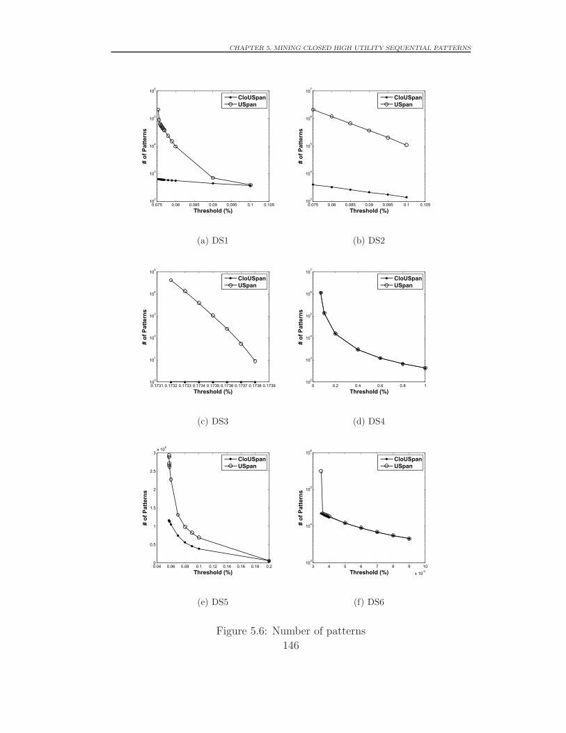
CHAPTER 5. MINING CLOSED HIGH UTILITY SEQUENTIAL PATTERNS
0.075 0.08 0.085 0.09 0.095 0.1 0.105102
103
104
105
106
# of
Pat
tern
s
Threshold (%)
CloUSpanUSpan
(a) DS1
0.075 0.08 0.085 0.09 0.095 0.1 0.105103
104
105
106
107
# of
Pat
tern
s
Threshold (%)
CloUSpanUSpan
(b) DS2
0.1731 0.1732 0.1733 0.1734 0.1735 0.1736 0.1737 0.1738 0.1739100
101
102
103
104
105
# of
Pat
tern
s
Threshold (%)
CloUSpanUSpan
(c) DS3
0 0.2 0.4 0.6 0.8 1102
103
104
105
106
107
# of
Pat
tern
s
Threshold (%)
CloUSpanUSpan
(d) DS4
0.04 0.06 0.08 0.1 0.12 0.14 0.16 0.18 0.20
0.5
1
1.5
2
2.5
3x 10⁵
# of
Pat
tern
s
Threshold (%)
CloUSpanUSpan
(e) DS5
3 4 5 6 7 8 9 10
x 10-3
103
104
105
106
# of
Pat
tern
s
Threshold (%)
CloUSpanUSpan
(f) DS6
Figure 5.6: Number of patterns
146

CHAPTER 5. MINING CLOSED HIGH UTILITY SEQUENTIAL PATTERNS
sion algorithm recovers the complete set of high utility sequences, which is
exactly the same as the output of USpan for all the experiments.
Clearly, all these figures indicate that CloUSpan losslessly reduces the
redundancy in the high utility sequential patterns, and substantially com-
presses the huge number of non-US-closed patterns to a very small group for
some datasets.
5.3.5 Pattern Length Distributions
Here we compare the pattern length distributions of CloUSpan and USpan
to further investigate how US-closed patterns represent non-US-closed. We
gather all the US-closed and non-US-closed patterns extracted by CloUSpan
and USpan separately for a certain threshold. For each pattern set, we count
the number of patterns with regard to their lengths, and plot the figures as
shown in Figure 5.7. The X axis means the pattern length and Y means the
number of patterns of that length.
Thousands of non-US-closed patterns may be generated from a single US-
closed pattern. This phenomenon can be found in Figure 5.7(a), 5.7(c), 5.7(e)
and 5.7(f). Instead of showing them all, CloUSpan presents a single pattern.
In Figure 5.7(b), the huge number of patterns can be actually represented
by several ones selected at the bottom. In Figure 5.7(d), US-closed patterns
absorb a few non-closed ones whose lengths are between.
Obviously, the pattern distribution shows that the proposed US-closed
representation has a massive reduction in the number of high utility sequen-
tial patterns.
In summary, CloUSpan discovers US-closed patterns with low redundan-
cy and less computational cost, and at the same time without losing any
information. Therefore, it is proven to be more valuable than USpan in all
aspects.
147

CHAPTER 5. MINING CLOSED HIGH UTILITY SEQUENTIAL PATTERNS
0 20 40 60 80 100 1200
0.5
1
1.5
2
2.5
3
3.5
4
4.5x 10⁴
# of
Pat
tern
s
Pattern Length
CloUSpanUSpan
(a) DS1 with ξ = 0.0754%
0 5 10 15 20 25 300
0.5
1
1.5
2
2.5
3x 10⁵
# of
Pat
tern
s
Pattern Length
CloUSpanUSpan
(b) DS2 with ξ = 0.075%
202 203 204 205 206 207 208 2090
2000
4000
6000
8000
10000
12000
14000
16000
18000
# of
Pat
tern
s
Pattern Length
CloUSpanUSpan
(c) DS3 with ξ = 0.1732%
0 10 20 30 40 50 60 70 800
1
2
3
4
5
6
7
8
9
10x 104
# of
Pat
tern
s
Pattern Length
CloUSpanUSpan
(d) DS4 ξ = 0.07%
100 101 102 1030
0.5
1
1.5
2
2.5
3
3.5
4
4.5
5x 10⁴
# of
Pat
tern
s
Pattern Length
CloUSpanUSpan
(e) DS5 ξ = 0.0572%
0 5 10 15 20 25 30 35 40100
101
102
103
104
105
# of
Pat
tern
s
Pattern Length
CloUSpanUSpan
(f) DS6 ξ = 0.0035%
Figure 5.7: Pattern length distributions
148

CHAPTER 5. MINING CLOSED HIGH UTILITY SEQUENTIAL PATTERNS
200 300 400 500 600 700 800 900 10000
500
1000
1500
2000
2500
3000
3500
4000
Tim
e(Se
c.)
Size of Database(k)
0.076%0.0756%
(a) DS1
200 300 400 500 600 700 800 900 10000
5000
10000
15000
Tim
e(Se
c.)
Size of Database(k)
0.1%0.08%
(b) DS2
Figure 5.8: Scalabilities
5.3.6 Scalability Test
The scalability test is conducted to test CloUSpan’s performance on large-
scale datasets. Sequence databases with 200K to 1000K sequences are gen-
erated from two synthetic datasets DS1 and DS2, with the same data distri-
bution characteristics described in Table 3.4. Figure 5.8 and Figure 5.9 show
the execution times and memory usages of the proposed CloUSpan approach
respectively on the datasets in terms of different data sizes and k values.
By setting different k values from 500 to 2000 on both datasets, both the
execution time and the memory usage are linear to the number of sequences.
5.4 Summary
In this chapter, we propose a compact and lossless representation of the com-
plete set of high utility sequential patterns, named US-closed high utility se-
quential patterns, to address the redundancy problem in high utility sequence
mining, which appears to be the first study on compact and lossless represen-
tation of high utility patterns, to the best of our knowledge. We prove and
validate the correctness of the proposed representation that can be recovered
149

CHAPTER 5. MINING CLOSED HIGH UTILITY SEQUENTIAL PATTERNS
200 300 400 500 600 700 800 900 1000100
200
300
400
500
600
700
Mem
ory
Usa
ge(M
B)
Size of Database(k)
0.076%0.0756%
(a) DS1
200 300 400 500 600 700 800 900 1000200
300
400
500
600
700
800
900
1000
Mem
ory
Usa
ge(M
B)
Size of Database(k)
0.1%0.08%
(b) DS2
Figure 5.9: Memory usage comparison
to the original pattern set without losing any information. To mine for the
new style of patterns, we propose an efficient algorithm, named CloUSpan.
Two effective strategies are further proposed to enhance the performance of
CloUSpan. We also implement a top-down method to efficiently recover all
high utility patterns from this representation. Experiments on both real and
synthetic datasets show that the proposed representation achieves a power-
ful lossless compression capability of high utility sequential patterns. It also
indicates that CloUSpan with the recovery method outperforms USpan, the
state-of-the-art algorithm of high utility sequence mining, to a great extent.
150

Chapter 6
Conclusions and Future Work
6.1 Conclusions
Sequential pattern mining is a very important issue in data mining and ma-
chine learning. Most traditional sequence mining focuses on extracting pat-
terns in the frequency/support framework which do not have business value
and impact, and thus are not actionable for business decision-making. The
introduction of “utility” not only brought valuable knowledge to sequence
analysis, but also new problems and challenges. First, the absence of the
Apriori Property in high utility sequence analysis makes the mining process
fundamentally different with frequent sequence mining. Novel structures and
algorithms need to be designed to improve performance and scalability, and
to conduct mining on platforms from industry level big data. Second, the
measurements of a pattern utility in a sequence might be different. For ex-
ample, in (Ahmed, Tanbeer, Jeong & Lee 2010), the authors define the utility
of a pattern as the sum of “all distinct occurrences” in a sequence. Different
utility calculation definitions will lead to completely different utility bound-
s, properties and pruning strategies. Third, according to our experience in
mining the utility sequence database, the extracted patterns also suffer from
a large amount of redundancy similar to frequent pattern mining . Many
patterns look very similar to one other. The challenge here is to explore
151
CHAPTER 6. CONCLUSIONS AND FUTURE WORK
approaches and algorithms which can efficiently and effectively summarize
the patterns, while losing only the smallest amount of information.
In Chapter 3, we provide a systematic statement of a generic framework
which defines calculations of the utility of a single item, an itemset, a sequence
and a sequence database. We specify a naive case from the framework which
uses the maximum utility calculation to extract high utility patterns. Based
on this, we present our solutions, including three utility bounds and the
corresponding pruning strategies, and two efficient algorithms USpan and
USpan+ were proposed. Substantial experiments on both synthetic and real
datasets show that the proposed algorithms efficiently identify high utility
sequences in large-scale data with low minimum utility.
In Chapter 4, we propose an efficient algorithm named TUS for mining
top-k high utility sequential patterns from utility-based sequence databases.
TUS guarantees that no sequence is missed during the mining process. We
develope a new sequence boundary and a corresponding pruning strategy for
effectively filtering unpromising candidates. Moreover, a pre-insertion and a
sorting strategy is introduced to raise the minimum utility threshold. The
mining performance is enhanced significantly since both the search space and
the number of candidates are effectively reduced by the proposed strategies.
Both synthetic and real datasets are used to evaluate the performance of
TUS, which is shown to substantially outperform the baseline algorithms,
and the performance of TUS is close to the optimal case of the state-of-the-
art utility sequential pattern mining algorithms.
In Chapter 5, we propose a compact and lossless representation of the
complete set of high utility sequential patterns, named US-closed high util-
ity sequential patterns, to address the redundancy problem in high utility
sequence mining. This appears to be the first study on compact and lossless
representation of high utility patterns, to the best of our knowledge. We
prove and validate the correctness of the proposed representation that can
be recovered to the original pattern set without losing any information. To
mine for the new style of patterns, we propose an efficient algorithm, named
152

CHAPTER 6. CONCLUSIONS AND FUTURE WORK
CloUSpan. Two effective strategies are proposed to enhance the performance
of CloUSpan. We also implement a top-down method to efficiently recover all
high utility patterns from this representation. Experiments on both real and
synthetic datasets show that the proposed representation achieves a power-
ful lossless compression capability of high utility sequential patterns. It also
indicates that CloUSpan with the recovery method significantly outperforms
USpan, the state-of-the-art algorithm of high utility sequence mining.
The limitation of the high utility sequential pattern mining framework is
that it is only target at mining a specific type of sequence. As discussed, a
sequence contains a series of events / itemsets. For complex sequences such
as time series, the proposed methods are incapable to process. Furthermore,
the utilities of the sequences are not allowed to be negative numbers, which
is not applicable in some real world applications. Another issue is that the
algorithms are unable to deal with very long sequences, or the execution time
of mining process grows exponentially in terms of the length of the sequences.
6.2 Future Work
High utility sequential pattern mining is very promising but still is at the
initial stage. Extensive work can be done to finalize the framework, as well
as extending to new areas, which include:
1. Summarization of high utility sequential patterns: We have im-
plemented lossless compression on the sequential patterns. However,
there is still much space for improvement in compressing the final re-
sultant patterns, which should be a lossy representation with an error
bound. With a new algorithm, the number of final patterns can be
greatly reduced and hopefully, performance can be significantly im-
proved.
2. The calculation of a sequence’s utility: In Chapter 2, we com-
pared different calculations of a sequence’s utility. All the works in this
153

CHAPTER 6. CONCLUSIONS AND FUTURE WORK
thesis use only one calculation. It would be worthwhile to explore other
calculations which have so far not been studied.
3. The coupling in utility-based sequence: This thesis only discusses
the utility-based sequence under the IID (Independent and Identical-
ly Distributed) assumption. In reality, sequences are coupled, which
presents a much more complicated than the case in this thesis. In the
future, we will redefine the problem in the non-IID framework, and will
study problems which have never before been encountered.
154
Bibliography
Agrawal, R., Imielinski, T. & Swami, A. (1993), Mining association rules
between sets of items in large databases, SIGMOD ’93, ACM, New
York, NY, USA, pp. 207–216.
Agrawal, R. & Shafer, J. C. (1996), ‘Parallel mining of association rules’,
Knowledge and Data Engineering, IEEE Transactions on 8(6), 962–969.
Agrawal, R. & Srikant, R. (1994), Fast algorithms for mining association
rules, VLDB ’94.
Agrawal, R. & Srikant, R. (1995), Mining sequential patterns, in ‘ICDE ’95.’,
pp. 3–14.
Ahmed, C. F., Tanbeer, S. K. & Jeong, B.-S. (2010a), Efficient mining of
high utility patterns over data streams with a sliding window method,
in R. Lee, J. Ma, L. Bacon, W. Du & M. Petridis, eds, ‘Software En-
gineering, Artificial Intelligence, Networking and Parallel/Distributed
Computing 2010’, Vol. 295 of Studies in Computational Intelligence,
Springer Berlin Heidelberg, pp. 99–113.
Ahmed, C. F., Tanbeer, S. K. & Jeong, B.-S. (2010b), Mining high utility
web access sequences in dynamic web log data, in ‘Software Engineering
Artificial Intelligence Networking and Parallel/Distributed Computing
(SNPD), 2010 11th ACIS International Conference on’, pp. 76–81.
Ahmed, C. F., Tanbeer, S. K., Jeong, B.-S. & Lee, Y.-K. (2008), Efficient
single-pass mining of weighted interesting patterns, in W. Wobcke &
155

BIBLIOGRAPHY
M. Zhang, eds, ‘AI 2008: Advances in Artificial Intelligence’, Vol. 5360
of Lecture Notes in Computer Science, Springer Berlin Heidelberg, p-
p. 404–415.
Ahmed, C. F., Tanbeer, S. K., Jeong, B.-S. & Lee, Y.-K. (2009a), ‘Efficient
tree structures for high utility pattern mining in incremental databases’,
Knowledge and Data Engineering, IEEE Transactions on 21(12), 1708–
1721.
Ahmed, C. F., Tanbeer, S. K., Jeong, B.-S. & Lee, Y.-K. (2010), ‘A novel ap-
proach for mining high-utility sequential patterns in sequence databas-
es’, ETRI Journal 32(5), 676–686.
Ahmed, C. F., Tanbeer, S. K., Jeong, B.-S., Lee, Y.-K. & Choi, H.-J. (2012),
‘Single-pass incremental and interactive mining for weighted frequent
patterns’, Expert Systems with Applications 39(9), 7976 – 7994.
Ahmed, C., Tanbeer, S., Jeong, B.-S. & Lee, Y.-K. (2009b), An efficient can-
didate pruning technique for high utility pattern mining, in T. Theer-
amunkong, B. Kijsirikul, N. Cercone & T.-B. Ho, eds, ‘Advances in
Knowledge Discovery and Data Mining’, Vol. 5476 of Lecture Notes in
Computer Science, Springer Berlin Heidelberg, pp. 749–756.
Ahmed, C., Tanbeer, S., Jeong, B.-S. & Lee, Y.-K. (2011), ‘Huc-prune: an
efficient candidate pruning technique to mine high utility patterns’, Ap-
plied Intelligence 34(2), 181–198.
Ayres, J., Flannick, J., Gehrke, J. & Yiu, T. (2002), Sequential pattern
mining using a bitmap representation, KDD ’02, ACM, New York, NY,
USA, pp. 429–435.
Birkhoff, G. (1967), Lattice Theory, third edn, American Mathematical So-
ciety.
156

BIBLIOGRAPHY
Cai, C. H., Fu, A.-C., Cheng, C. & Kwong, W. W. (1998), Mining association
rules with weighted items, in ‘Proceedings. IDEAS’98. International’,
pp. 68–77.
Calders, T. & Goethals, B. (2002), Mining all non-derivable frequent item-
sets, in T. Elomaa, H. Mannila & H. Toivonen, eds, ‘Principles of Data
Mining and Knowledge Discovery’, Vol. 2431 of Lecture Notes in Com-
puter Science, Springer Berlin Heidelberg, pp. 74–86.
Cao, L. (2009), Actionable Knowledge Discovery, IGI Global.
Cao, L. (2012), ‘Actionable knowledge discovery and delivery’, Wiley Inter-
disciplinary Reviews: Data Mining and Knowledge Discovery 2(2), 149–
163.
Cao, L., Yu, P., Zhang, C. & Zhang, H. (2008), Data mining for business
applications, Springer.
Cao, L. & Zhang, C. (2006), Domain-driven actionable knowledge discov-
ery in the real world, in ‘Advances in Knowledge Discovery and Data
Mining’, Springer, pp. 821–830.
Cao, L., Zhao, Y., Zhang, H., Luo, D., Zhang, C. & Park, E. K. (2010),
‘Flexible frameworks for actionable knowledge discovery’, Knowledge
and Data Engineering, IEEE Transactions on 22(9), 1299–1312.
Chan, R., Yang, Q. & Shen, Y.-D. (2003), Mining high utility itemsets, in
‘Data Mining, 2003. ICDM 2003. Third IEEE International Conference
on’, pp. 19–26.
Chang, J. H. (2011), ‘Mining weighted sequential patterns in a se-
quence database with a time-interval weight’, Knowledge-Based Systems
24(1), 1–9.
157

BIBLIOGRAPHY
Cheung, D., Han, J., Ng, V., Fu, A. W. & Fu, Y. (1996), A fast distribut-
ed algorithm for mining association rules, in ‘Parallel and Distributed
Information Systems, Fourth International Conference on’, pp. 31–42.
Cheung, D. W.-L., Han, J., Ng, V. & Wong, C. Y. (1996), Maintenance of
discovered association rules in large databases: An incremental updating
technique, in ‘Proceedings of the Twelfth International Conference on
Data Engineering’, ICDE ’96, IEEE Computer Society, Washington,
DC, USA, pp. 106–114.
Cheung, W. & Zaiane, O. (2003), Incremental mining of frequent patterns
without candidate generation or support constraint, in ‘Database En-
gineering and Applications Symposium. Proceedings. Seventh Interna-
tional’, pp. 111–116.
Cheung, Y.-L. & Fu, A.-C. (2004), ‘Mining frequent itemsets without support
threshold: with and without item constraints’, Knowledge and Data
Engineering, IEEE Transactions on 16(9), 1052–1069.
Chiu, D.-Y., Wu, Y.-H. & Chen, A. (2004), An efficient algorithm for min-
ing frequent sequences by a new strategy without support counting, in
‘ICDE 2004’, pp. 375–386.
Chu, C.-J., Tseng, V. S. & Liang, T. (2008), ‘An efficient algorithm for
mining temporal high utility itemsets from data streams’, Journal of
Systems and Software 81(7), 1105–1117.
Chuang, K.-T., Huang, J.-L. & Chen, M.-S. (2008), ‘Mining top-k frequent
patterns in the presence of the memory constraint’, The VLDB Journal
17(5), 1321–1344.
Cong, S., Han, J. & Padua, D. (2005), Parallel mining of closed sequential
patterns, in ‘Proceedings of the Eleventh ACM SIGKDD International
Conference on Knowledge Discovery in Data Mining’, KDD ’05, ACM,
New York, NY, USA, pp. 562–567.
158

BIBLIOGRAPHY
Davey, B. A. & Priestley, H. A. (1994), Introduction to Lattices and Order,
third edn, Cambridge University Press.
Erwin, A., Gopalan, R. & Achuthan, N. (2008), Efficient mining of high u-
tility itemsets from large datasets, in T. Washio, E. Suzuki, K. Ting
& A. Inokuchi, eds, ‘Advances in Knowledge Discovery and Data Min-
ing’, Vol. 5012 of Lecture Notes in Computer Science, Springer Berlin
Heidelberg, pp. 554–561.
Erwin, A., Gopalan, R. P. & Achuthan, N. R. (2007a), A bottom-up projec-
tion based algorithm for mining high utility itemsets, in ‘Proceedings
of the 2Nd International Workshop on Integrating Artificial Intelligence
and Data Mining - Volume 84’, AIDM ’07, Australian Computer Society,
Inc., Darlinghurst, Australia, Australia, pp. 3–11.
Erwin, A., Gopalan, R. P. & Achuthan, N. R. (2007b), Ctu-mine: An ef-
ficient high utility itemset mining algorithm using the pattern growth
approach, in ‘Computer and Information Technology, 2007. CIT 2007.
7th IEEE International Conference on’, pp. 71–76.
Fournier-Viger, P., Wu, C.-W., Zida, S. & Tseng, V. S.-M. (2014), Fhm:
Faster high-utility itemset mining using estimated utility co-occurrence
pruning, in ‘Foundations of Intelligent Systems’, Vol. 8502 of Lecture
Notes in Computer Science, Springer International Publishing.
Grahne, G. & Zhu, J. (2003), Efficiently using prefix-trees in mining frequent
itemsets., in ‘FIMI’, Vol. 3, pp. 123–132.
Han, J. (2005), Data Mining: Concepts and Techniques, Morgan Kaufmann
Publishers Inc., San Francisco, CA, USA.
Han, J., Pei, J., Mortazavi-Asl, B., Chen, Q., Dayal, U. & Hsu, M.-C. (2000),
Freespan: frequent pattern-projected sequential pattern mining, KDD
’00, ACM, New York, NY, USA, pp. 355–359.
159

BIBLIOGRAPHY
Han, J., Pei, J. & Yin, Y. (2000), Mining frequent patterns without candidate
generation, SIGMOD ’00, ACM, New York, NY, USA, pp. 1–12.
Han, J., Wang, J., Lu, Y. & Tzvetkov, P. (2002), Mining top-k frequent closed
patterns without minimum support, in ‘Data Mining. Proceedings IEEE
International Conference on’, pp. 211–218.
Heckerman, D. (1999), ‘Msnbc.com anonymous web data data set’,
http://archive.ics.uci.edu/ml/datasets/MSNBC.com+Anonymous+
Web+Data.
Hong, T.-P., Lin, C.-W. & Wu, Y.-L. (2008), ‘Incrementally fast updated
frequent pattern trees’, Expert Systems with Applications 34(4), 2424 –
2435.
Huang, K.-Y., Chang, C.-H., Tung, J.-H. & Ho, C.-T. (2006), Cobra: Closed
sequential pattern mining using bi-phase reduction approach, in A. Tjoa
& J. Trujillo, eds, ‘Data Warehousing and Knowledge Discovery’, Vol.
4081 of Lecture Notes in Computer Science, Springer Berlin Heidelberg,
pp. 280–291.
Koh, J.-L. & Shieh, S.-F. (2004), An efficient approach for maintaining as-
sociation rules based on adjusting fp-tree structures, in Y. Lee, J. Li,
K.-Y. Whang & D. Lee, eds, ‘Database Systems for Advanced Applica-
tions’, Vol. 2973 of Lecture Notes in Computer Science, Springer Berlin
Heidelberg, pp. 417–424.
Lan, G.-C., Hong, T.-P., Huang, H.-C. & Pan, S.-T. (2013), Mining high
fuzzy utility sequential patterns, in ‘Fuzzy Theory and Its Applications
(iFUZZY), 2013 International Conference on’, pp. 420–424.
Lan, G.-C., Hong, T.-P., Tseng, V. S. & Wang, S.-L. (2014), ‘Applying
the maximum utility measure in high utility sequential pattern mining’,
Expert Systems with Applications 41(11), 5071–5081.
160
BIBLIOGRAPHY
Lee, G. & Yun, U. (2012), Mining weighted frequent sub-graphs with weight
and support affinities, in C. Sombattheera, N. Loi, R. Wankar &
T. Quan, eds, ‘Multi-disciplinary Trends in Artificial Intelligence’, Vol.
7694 of Lecture Notes in Computer Science, Springer Berlin Heidelberg,
pp. 224–235.
Leggett, J. J. & Yun, U. (2005), Wfim: Weighted frequent itemset mining
with a weight range and a minimum weight, in ‘Proceedings of the 2005
SIAM International Conference on Data Mining’, pp. 636–640.
Leung, C.-S., Khan, Q., Li, Z. & Hoque, T. (2007), ‘Cantree: a canonical-
order tree for incremental frequent-pattern mining’, Knowledge and In-
formation Systems 11(3), 287–311.
Li, H.-F., Huang, H.-Y., Chen, Y.-C., Liu, Y.-J. & Lee, S.-Y. (2008), Fast
and memory efficient mining of high utility itemsets in data streams, in
‘Data Mining, 2008. ICDM ’08. Eighth IEEE International Conference
on’, pp. 881–886.
Li, X., Deng, Z.-H. & Tang, S. (2006), A fast algorithm for maintenance of
association rules in incremental databases, in X. Li, O. Zaiane & Z.-h.
Li, eds, ‘Advanced Data Mining and Applications’, Vol. 4093 of Lecture
Notes in Computer Science, Springer Berlin Heidelberg, pp. 56–63.
Li, Y.-c. & Yeh, J.-s. (2005), Efficient algorithms for mining share-frequent
itemsets, in ‘In Proceedings of the 11th World Congress of Intl. Fuzzy
Systems Association’, p. 0534V539.
Li, Y.-C., Yeh, J.-S. & Chang, C.-C. (2005), Direct candidates generation:
A novel algorithm for discovering complete share-frequent itemsets, in
L. Wang & Y. Jin, eds, ‘Fuzzy Systems and Knowledge Discovery’, Vol.
3614, Springer Berlin Heidelberg, pp. 551–560.
161

BIBLIOGRAPHY
Li, Y.-C., Yeh, J.-S. & Chang, C.-C. (2008), ‘Isolated items discarding strate-
gy for discovering high utility itemsets’, Data & Knowledge Engineering
64(1), 198–217.
Lin, C.-W., Hong, T.-P., Lan, G.-C., Chen, H.-Y. & Kao, H.-Y. (2010),
Incrementally mining high utility itemsets in dynamic databases, in
‘Granular Computing (GrC), 2010 IEEE International Conference on’,
pp. 303–307.
Lin, C.-W., Hong, T.-P., Lan, G.-C., Wong, J.-W. & Lin, W.-Y. (2013),
Mining high utility itemsets based on the pre-large concept, in R.-S.
Chang, L. C. Jain & S.-L. Peng, eds, ‘Advances in Intelligent Systems
and Applications - Volume 1’, Vol. 20 of Smart Innovation, Systems and
Technologies, Springer Berlin Heidelberg, pp. 243–250.
Lin, C.-W., Hong, T.-P., Lan, G.-C., Wong, J.-W. & Lin, W.-Y. (2014),
‘Incrementally mining high utility patterns based on pre-large concept’,
Applied Intelligence 40(2), 343–357.
Lin, C.-W., Lan, G.-C. & Hong, T.-P. (2012), ‘An incremental mining al-
gorithm for high utility itemsets’, Expert Systems with Applications
39(8), 7173–7180.
Liu, J., Wang, K. & Fung, B. (2012), Direct discovery of high utility itemsets
without candidate generation, in ‘Data Mining (ICDM), 2012 IEEE 12th
International Conference on’, pp. 984–989.
Liu, M. & Qu, J. (2012), Mining high utility itemsets without candidate
generation, in ‘Proceedings of the 21st ACM International Conference
on Information and Knowledge Management’, CIKM ’12, ACM, New
York, NY, USA, pp. 55–64.
Liu, Y., Liao, W.-k. & Choudhary, A. (2005a), A fast high utility itemsets
mining algorithm, in ‘Proceedings of the 1st International Workshop on
162

BIBLIOGRAPHY
Utility-based Data Mining’, UBDM ’05, ACM, New York, NY, USA,
pp. 90–99.
Liu, Y., Liao, W.-k. & Choudhary, A. (2005b), A two-phase algorithm for
fast discovery of high utility itemsets, in T. Ho, D. Cheung & H. Liu,
eds, ‘Advances in Knowledge Discovery and Data Mining’, Vol. 3518
of Lecture Notes in Computer Science, Springer Berlin Heidelberg, p-
p. 689–695.
Lucchese, C., Orlando, S. & Perego, R. (2006), ‘Fast and memory efficient
mining of frequent closed itemsets’, Knowledge and Data Engineering,
IEEE Transactions on 18(1), 21–36.
Lucchese, C., Orlando, S. & Perego, R. (2007), Parallel mining of frequent
closed patterns: Harnessing modern computer architectures, in ‘Data
Mining, 2007. ICDM 2007. Seventh IEEE International Conference on’,
pp. 242–251.
Mabroukeh, N. R. & Ezeife, C. I. (2010), ‘A taxonomy of sequential pattern
mining algorithms’, ACM Comput. Surv. 43, 1–41.
Microsoft (2008), ‘Microsoft sql server 2008 food mart database’,
http://www.informit.com/store/microsoft-sql-server-2008-analysis-
services-unleashed-9780672330018.
Mooney, C. H. & Roddick, J. F. (2013), ‘Sequential pattern mining – ap-
proaches and algorithms’, ACM Comput. Surv. 45(2), 1–39.
Park, J. S., Chen, M.-S. & Yu, P. S. (1995), An effective hash-based algorithm
for mining association rules, in ‘Proceedings of the 1995 ACM SIGMOD
International Conference on Management of Data’, SIGMOD ’95, ACM,
New York, NY, USA, pp. 175–186.
Pasquier, N., Bastide, Y., Taouil, R. & Lakhal, L. (1999), Discovering fre-
quent closed itemsets for association rules, in C. Beeri & P. Buneman,
163
BIBLIOGRAPHY
eds, ‘Database Theory ICDT 1999’, Vol. 1540 of Lecture Notes in Com-
puter Science, Springer Berlin Heidelberg, pp. 398–416.
Pei, J., Han, J., Behzad, M.-A., Wang, J., Pinto, H., Chen, Q., Dayal, U.
& Hsu, M.-C. (2004), ‘Mining sequential patterns by pattern-growth:
the prefixspan approach’, IEEE Transactions on Knowledge and Data
Engineering 16(11), 1424–1440.
Pei, J., Han, J. & Mao, R. (2000), Closet: An efficient algorithm for min-
ing frequent closed itemsets, in ‘ACM SIGMOD Workshop on Research
Issues in Data Mining and Knowledge Discovery’00’, pp. 21–30.
Pei, J., Han, J., Mortazavi-Asl, B., Pinto, H., Chen, Q., Dayal, U. & Hsu, M.-
C. (2001), Prefixspan: mining sequential patterns efficiently by prefix-
projected pattern growth, in ‘Data Engineering, 2001. Proceedings. 17th
International Conference on’, pp. 215–224.
Pisharath, J., Liu, Y., Ozisikyilmaz, B., Narayanan, R., Liao, W.,
Choudhary, A. & Memik, G. (2005), ‘Nu-minebench version
2.0 dataset and technical report’, http://cucis.ece.northwestern.ed-
u/projects/DMS/MineBench.html.
Quang, T., Oyanagi, S. & Yamazaki, K. (2006), Exminer: An efficient algo-
rithm for mining top-k frequent patterns, in X. Li, O. Zaiane & Z.-h.
Li, eds, ‘Advanced Data Mining and Applications’, Vol. 4093 of Lecture
Notes in Computer Science, Springer Berlin Heidelberg, pp. 436–447.
Savasere, A., Omiecinski, E. & Navathe, S. (1995), An efficient algorithm for
mining association rules in large databases, VLDB ’95, pp. 432–443.
Shie, B.-E., Cheng, J.-H., Chuang, K.-T. & Tseng, V. S. (2012), A one-phase
method for mining high utility mobile sequential patterns in mobile com-
merce environments, in H. Jiang, W. Ding, M. Ali & X. Wu, eds, ‘Ad-
vanced Research in Applied Artificial Intelligence’, Vol. 7345 of Lecture
Notes in Computer Science, Springer Berlin Heidelberg, pp. 616–626.
164

BIBLIOGRAPHY
Shie, B.-E., Hsiao, H.-F., Tseng, V. & Yu, P. (2011), Mining high utility
mobile sequential patterns in mobile commerce environments, in J. Yu,
M. Kim & R. Unland, eds, ‘Database Systems for Advanced Applica-
tions’, Vol. 6587 of Lecture Notes in Computer Science, Springer Berlin
Heidelberg, pp. 224–238.
Shie, B.-E., Tseng, V. S. & Yu, P. S. (2010), Online mining of temporal
maximal utility itemsets from data streams, in ‘Proceedings of the 2010
ACM Symposium on Applied Computing’, SAC ’10, ACM, New York,
NY, USA, pp. 1622–1626.
Shie, B.-E., Yu, P. & Tseng, V. (2013), ‘Mining interesting user behav-
ior patterns in mobile commerce environments’, Applied Intelligence
38(3), 418–435.
SIGKDD (2000), ‘Kdd cup 2000: Online retailer website clickstream
analysis’, http://www.sigkdd.org/kdd-cup-2000-online-retailer-website-
clickstream-analysis.
Song, W., Liu, Y. & Li, J. (2012), Vertical mining for high utility itemsets, in
‘Granular Computing (GrC), 2012 IEEE International Conference on’,
pp. 429–434.
Song, W., Liu, Y. & Li, J. (2014), ‘Mining high utility itemsets by dynami-
cally pruning the tree structure’, Applied Intelligence 40(1), 29–43.
Srikant, R. & Agrawal, R. (1996), Mining sequential patterns: Generaliza-
tions and performance improvements, in ‘Advances in Database Tech-
nology EDBT ’96’, Vol. 1057, Springer Berlin Heidelberg, pp. 1–17.
Sun, K. & Bai, F. (2008), ‘Mining weighted association rules without preas-
signed weights’, Knowledge and Data Engineering, IEEE Transactions
on 20(4), 489–495.
165

BIBLIOGRAPHY
Tanbeer, S., Ahmed, C., Jeong, B.-S. & Lee, Y.-K. (2008), Cp-tree: A tree
structure for single-pass frequent pattern mining, in T. Washio, E. Suzu-
ki, K. Ting & A. Inokuchi, eds, ‘Advances in Knowledge Discovery and
Data Mining’, Vol. 5012 of Lecture Notes in Computer Science, Springer
Berlin Heidelberg, pp. 1022–1027.
Tao, F., Murtagh, F. & Farid, M. (2003), Weighted association rule min-
ing using weighted support and significance framework, in ‘Proceedings
of the Ninth ACM SIGKDD International Conference on Knowledge
Discovery and Data Mining’, KDD ’03, ACM, New York, NY, USA,
pp. 661–666.
Toivonen, H. (1996), Sampling large databases for association rules, in
‘Proceedings of the 22th International Conference on Very Large Data
Bases’, VLDB ’96, Morgan Kaufmann Publishers Inc., San Francisco,
CA, USA, pp. 134–145.
Tseng, V. S., Chu, C.-J. & Liang, T. (2006), Efficient mining of temporal
high utility itemsets from data streams, in ‘Proceedings of the 2nd In-
ternational Workshop on Utility-based Data Mining’, UBDM ’06, ACM,
New York, NY, USA.
Tseng, V. S., Wu, C.-W., Shie, B.-E. & Yu, P. S. (2010), Up-growth: An
efficient algorithm for high utility itemset mining, in ‘Proceedings of the
16th ACM SIGKDD International Conference on Knowledge Discovery
and Data Mining’, KDD ’10, ACM, New York, NY, USA, pp. 253–262.
Tseng, V., Shie, B.-E., Wu, C.-W. & Yu, P. (2013), ‘Efficient algorithms for
mining high utility itemsets from transactional databases’, Knowledge
and Data Engineering, IEEE Transactions on 25(8), 1772–1786.
Tzvetkov, P., Yan, X. & Han, J. (2005), ‘Tsp: Mining top-k closed sequential
patterns’, Knowledge and Information Systems 7(4), 438–457.
166

BIBLIOGRAPHY
Wang, J. & Han, J. (2004), Bide: efficient mining of frequent closed se-
quences, in ‘Data Engineering, 2004. Proceedings. 20th International
Conference on’, pp. 79–90.
Wang, J., Han, J., Lu, Y. & Tzvetkov, P. (2005), ‘Tfp: an efficient algo-
rithm for mining top-k frequent closed itemsets’, Knowledge and Data
Engineering, IEEE Transactions on 17(5), 652–663.
Wang, J., Han, J. & Pei, J. (2003), Closet+: Searching for the best strategies
for mining frequent closed itemsets, in ‘Proceedings of the Ninth ACM
SIGKDD International Conference on Knowledge Discovery and Data
Mining’, KDD ’03, ACM, New York, NY, USA, pp. 236–245.
Wang, W., Yang, J. & Yu, P. S. (2000), Efficient mining of weighted asso-
ciation rules (war), in ‘Proceedings of the Sixth ACM SIGKDD Inter-
national Conference on Knowledge Discovery and Data Mining’, KDD
’00, ACM, New York, NY, USA, pp. 270–274.
Wu, C.-W., Fournier-Viger, P., Yu, P. S. & Tseng, V. S. (2011), Efficient
mining of a concise and lossless representation of high utility itemsets,
in ‘Data Mining (ICDM), 2011 IEEE 11th International Conference on’,
pp. 824–833.
Wu, C.-W., Lin, Y.-F., Yu, P. S. & Tseng, V. S. (2013), Mining high utility
episodes in complex event sequences, in ‘Proceedings of the 19th ACM
SIGKDD International Conference on Knowledge Discovery and Data
Mining’, KDD ’13, ACM, New York, NY, USA, pp. 536–544.
Wu, C. W., Shie, B.-E., Tseng, V. S. & Yu, P. S. (2012), Mining top-k high
utility itemsets, in ‘Proceedings of the 18th ACM SIGKDD International
Conference on Knowledge Discovery and Data Mining’, KDD ’12, ACM,
New York, NY, USA, pp. 78–86.
167

BIBLIOGRAPHY
Yan, X., Han, J. & Afshar, R. (2003), Clospan: Mining: Closed sequential
patterns in large datasets, in ‘Proceedings of the 2003 SIAM Interna-
tional Conference on Data Mining’, pp. 166–177.
Yang, Z., Kitsuregawa, M. & Wang, Y. (2006), Paid: Mining sequential
patterns by passed item deduction in large databases, in ‘Database En-
gineering and Applications Symposium, 2006. IDEAS ’06. 10th Interna-
tional’, pp. 113–120.
Yang, Z., Wang, Y. & Kitsuregawa, M. (2007), Lapin: Effective sequential
pattern mining algorithms by last position induction for dense databas-
es, in ‘Advances in Databases: Concepts, Systems and Applications’,
Vol. 4443 of Lecture Notes in Computer Science, pp. 1020–1023.
Yao, H., Hamilton, H. J. & Butz, C. J. (2004), A foundational approach to
mining itemset utilities from databases, in ‘Proceedings of the Third
SIAM International Conference on Data Mining’, pp. 482–486.
Yen, S.-J. & Lee, Y.-S. (2007), Mining high utility quantitative association
rules, in I. Song, J. Eder & T. Nguyen, eds, ‘Data Warehousing and
Knowledge Discovery’, Vol. 4654 of Lecture Notes in Computer Science,
Springer Berlin Heidelberg, pp. 283–292.
Yin, J., Zheng, Z. & Cao, L. (2012), Uspan: An efficient algorithm for min-
ing high utility sequential patterns, in ‘Proceedings of the 18th ACM
SIGKDD International Conference on Knowledge Discovery and Data
Mining’, KDD ’12, ACM, New York, NY, USA, pp. 660–668.
Yun, U. (2007a), ‘Efficient mining of weighted interesting patterns
with a strong weight and/or support affinity’, Information Sciences
177(17), 3477–3499.
Yun, U. (2007b), ‘Mining lossless closed frequent patterns with weight con-
straints’, Knowledge-Based Systems 20(1), 86–97.
168

BIBLIOGRAPHY
Yun, U. (2008a), ‘An efficient mining of weighted frequent patterns
with length decreasing support constraints’, Knowledge-Based Systems
21(8), 741–752.
Yun, U. (2008b), ‘A new framework for detecting weighted sequential patterns
in large sequence databases’, Knowledge-Based Systems 21(2), 110 –
122.
Yun, U. & Leggett, J. (2006a), Wspan: Weighted sequential pattern mining
in large sequence databases, in ‘Intelligent Systems, 2006 3rd Interna-
tional IEEE Conference on’, pp. 512–517.
Yun, U. & Leggett, J. J. (2005), Wlpminer: Weighted frequent pattern min-
ing with length-decreasing support constraints, in T. Ho, D. Cheung &
H. Liu, eds, ‘Advances in Knowledge Discovery and Data Mining’, Vol.
3518 of Lecture Notes in Computer Science, Springer Berlin Heidelberg,
pp. 555–567.
Yun, U. & Leggett, J. J. (2006b), Wip: Mining weighted interesting patterns
with a strong weight and/or support affinity, in ‘In Proceedings of the
Sixth SIAM International Conference on Data Mining’.
Yun, U., Shin, H., Ryu, K. H. & Yoon, E. (2012), ‘An efficient mining algo-
rithm for maximal weighted frequent patterns in transactional databas-
es’, Knowledge-Based Systems 33(0), 53–64.
Zaki, M. (2000), ‘Scalable algorithms for association mining’, Knowledge and
Data Engineering, IEEE Transactions on 12(3), 372–390.
Zaki, M. & Hsiao, C.-J. (2005), ‘Efficient algorithms for mining closed item-
sets and their lattice structure’, Knowledge and Data Engineering, IEEE
Transactions on 17(4), 462–478.
Zaki, M. J. (2001), ‘Spade: An efficient algorithm for mining frequent se-
quences’, Machine Learning 42, 31–60.
169

BIBLIOGRAPHY
Zaki, M. J. & Hsiao, C.-J. (2002), Charm: An efficient algorithm for closed
itemset mining, in ‘Proceedings of the 2002 SIAM International Confer-
ence on Data Mining’, pp. 457–473.
Zaki, M. J., Parthasarathy, S., Ogihara, M. & Li, W. (1997), ‘Parallel algo-
rithms for discovery of association rules’, Data Mining and Knowledge
Discovery 1(4), 343–373.
Zhou, L., Liu, Y., Wang, J. & Shi, Y. (2007), Utility-based web path traversal
pattern mining, in ‘Data Mining Workshops, 2007. ICDM Workshops
2007. Seventh IEEE International Conference on’, pp. 373–380.
170