mining residue contacts in proteins using local structure ...zaki/paperdir/tsmc03.pdf · ieee...

IEEE TRANSACTIONS ON SYSTEMS, MAN, AND CYBERNETICS—PART B: CYBERNETICS, VOL. 33, NO. 5, OCTOBER 2003 789

Mining Residue Contacts in Proteins UsingLocal Structure Predictions

Mohammed J. Zaki, Associate Member, IEEE, Shan Jin, and Chris Bystroff

Abstract—In this paper we develop data mining techniques topredict three-dimensional (3-D) contact potentials among proteinresidues (or amino acids) based on the hierarchical nucleation-propagation model of protein folding. We apply a hybrid approach,using a hidden Markov model to extract folding initiation sites, andthen apply association mining to discover contact potentials. Thenew hybrid approach achieves accuracy results better than thosereported previously.

Index Terms—Association rules, contact maps, data mining,hidden Markov models, protein structure prediction.

I. INTRODUCTION

B IOINFORMATICS is the science of storing, extracting,organizing, analyzing, interpreting, and utilizing infor-

mation from biological sequences and molecules. It has beenmainly fueled by advances in DNA sequencing and genomemapping techniques. The Human Genome Project has resultedin rapidly growing databases of genetic sequences, while theStructural Genomics Initiative is doing the same for the proteinstructure database. New techniques are needed to analyze,manage, and discover sequence, structure, and functionalpatterns, or models, from these large sequence and structuraldatabases. High performance data analysis algorithms are alsobecoming central to this task.

Bioinformatics is an emerging field, undergoing rapid and ex-citing growth. Knowledge discovery and data mining (KDD)techniques will play an increasingly important role in the anal-ysis and discovery of sequence, structure and functional pat-terns or models from large sequence databases. One of the grandchallenges of bioinformatics still remains, namely, the proteinfolding problem.

Proteins fold spontaneously and reproducibly (on a time scaleof milliseconds) into complex 3-D globules when placed in anaqueous solution, and, the sequence of amino acids making upa protein appears to completely determine its three dimensionalstructure. Given a protein amino acid sequence (linear struc-ture), determining its 3-D folded shape, (tertiary structure), isreferred to as thestructure prediction problem; it is widely ac-

Manuscript received June 28, 2001; revised October 17, 2002. This work wassupported in part by the National Science Foundation under CAREER AwardIIS-0092978, the National Science Foundation under Next Generation SoftwareProgram grant EIA-0103708, and the Department of Energy Early Career AwardDE-FG02-02ER25538. This paper was recommended by Guest Editor N. Bour-bakis.

M. J. Zaki and S. Jin are with the Computer Science Department, RensselaerPolytechnic Institute, Troy, NY 12180 USA (e-mail: zaki@cs. rpi.edu, [email protected]).

C. Bystroff is with the Biology Department, Rensselaer Polytechnic Institute,Troy, NY 12180 USA (e-mail: [email protected]).

Digital Object Identifier 10.1109/TSMCB.2003.816916

knowledged as an open problem, and a lot of research in the pasthas focused on it.

Traditional approaches to protein structure prediction havefocused on detection of evolutionary homology [2], fold recog-nition [3], [21], and where those fail, ab initio simulations [22]that generally perform a conformational search for the lowestenergy state [20]. However, the conformational search space ishuge, and, if nature approached the problem using a completesearch, a protein would take longer to fold than the age of theuniverse, while proteins are observed to fold in milliseconds.Thus, a structured folding pathway (time ordered sequence offolding events) must play an important role in this conforma-tional search. Strong experimental evidence for pathway-basedmodels of protein folding has emerged over the years, for ex-ample, experiments revealing the structure of the “unfolded”state in water [15], burst-phase folding intermediates [6], andthe kinetic effects of point mutations (“phi-values” [16]). Thesepathway models indicate that certain events always occur earlyin the folding process and certain others always occur later.

It appears that the traditional approaches, while having pro-vided considerable insight into the chemistry and biology offolding have largely hit a brick wall when it comes to structureprediction, hence, a novel approach is called for, for example,using data mining. Mining from examples is a data driven ap-proach that is generally useful when physical models are in-tractable or unknown, however, data representing the processis available. Thus, our problem appears to be ideally suited tothe application of mining—physical models of folding are ei-ther intractable or not well understood, and data in the form ofa protein data base exists.

II. M ODELING PROTEIN FOLDING

It is well known that proteins fold spontaneously and repro-ducibly to a unique 3-D structure in aqueous solution. Despitesignificant advances in recent years, the goal of predicting the3-D structure of a protein from its one-dimensional (1-D) se-quence of amino acids, without the aid of evolutionary infor-mation, remains one of greatest and most elusive challenges inbioinformatics. The current state of the art in structure predic-tion provides insights that guide further experimentation, butfalls far short of replacing those experiments.

Today we are witnessing a paradigm shift in predictingprotein structure from its known amino acid sequence

. The traditional or Ab initio folding methodemployed first principles to derive the 3-D structure of proteins.However, even though considerable progress has been made inunderstanding the chemistry and biology of folding, the successof ab initio folding has been quite limited.

1083-4419/03$17.00 © 2003 IEEE

790 IEEE TRANSACTIONS ON SYSTEMS, MAN, AND CYBERNETICS—PART B: CYBERNETICS, VOL. 33, NO. 5, OCTOBER 2003

Instead of simulation studies, an alternative approach is toemploy learning from examples using a database of known pro-tein structures. For example, the Brookhaven Protein Database(PDB) records the 3-D coordinates of the atoms of thousandsof protein structures. Most of these proteins cluster into around700 fold-families based on their similarity. It is conjectured thatthere will be on the order of 1000 fold-families for the nat-ural proteins [25]. The PDB thus offers a new paradigm to pro-tein structure prediction by employing data mining methodslike clustering, classification, association rules, hidden Markovmodels, etc.

A fascinating property of protein chains is that they spon-taneously and reproducibly fold themselves into complexthree-dimensional globules when placed in an aqueous solu-tion. The sequence of amino acids making up the polypeptidechain contains, encoded within it, the complete buildinginstructions. This self-organization cannot occur by a randomconformational search for the lowest energy state [12], sincesuch a search would take millions of years, while proteins foldin milliseconds. In recent years, a combination of molecularbiological and biophysical techniques have dissected thefolding process into fast and slow components which localizeto certain parts of the amino acid sequence [19].

A. I-Sites Motifs and HMMSTR

Some small, fast-folding regions of the molecule may beidentified by their sequence alone. A library of short sequencepatterns that fold fast has been compiled by cluster analysis ofthe database of known protein structures (the I-sites Library,[4]). In this work, similar short sequences that mapped to thesame local structure in different proteins were deemed to be au-tonomous folding units, and the short sequences were compiledinto patterns or “profiles” which could then be used to predictwhether or not a segment of the protein would tend to fold inde-pendently of the rest of the molecule. Cross-validation showeda strong statistical significance to the predictions made by theprofiles, and later NMR studies showed that some peptidespredicted to fold in isolation actually did so [27]. Peptides witha strong tendency to fold independently constitute about 30%of the amino acid residues in protein sequences. The formationof independent folding units (I-sites motifs) is the first level ofself-organization in the folding process: the “initiation.”

These short motifs occur in proteins of widely differingtopology, and so cannot contain sufficient information to definethe overall, global fold of the protein molecule. Moreover,they are too short to be the fast-folding regions found byexperimental dissection. There must be a higher level ofself-organization which dictates how the short pieces cometogether to form larger, longer globular domains. The rulesdefining the propagation of structure along the chain, startingfrom the sites of initiation, have been extracted from the data-base of known protein structures and formalized as a hiddenMarkov model (HMM), called HMMSTR [5] (or “hamster”),discussed further below. HMMSTR models the interactionsbetween adjacent short regions of the sequence, and so attemptsto model the second level of self-organization: “propagation”of structure along the sequence.

The I-sites Library models the initiation sites of folding, andthe new HMM models interactions between those sites. ButHMMSTR [5] is a network of connections between I-sites mo-tifs, and thus simultaneously models both folding initiation andpropagation. The two levels of complexity, not discretely de-fined but smoothly intermingled, are represented in the HMM asvariable degrees of branching. Unbranched segments are initia-tions sites, whose probabilities depend simultaneously on shortcontiguous segments of the sequence, while branching and cy-cles represent multiple sequence-dependent ways of extendingand linking the initiation sites. Arbitrary levels of complexitymay be modeled by including HMMs recursively within over-arching HMMs, the latter representing the ways of connectingthe output of the HMMs it contains. Hidden Markov models arelimited to data that can be expressed as 1-D sequences of dis-crete symbols, but there are techniques for overcoming both thediscreteness and the one-dimensionality [18].

The next level of complexity in protein folding is called “con-densation.” In the first few microseconds after introducing thepolypeptide chain into an aqueous solution, initiation sites formtransient, rapidly-interchanging structures, favoring one or moreconformations to varying degrees. These structures propagatealong the chain by promoting compatible upstream and down-stream conformations, and the resulting transiently-formed sub-structures encounter each other by through-space diffusion, con-densing into larger, ordered globules, as energy dictates. The or-dering of these three processes is not discrete but overlapping,and they should therefore be integrated into a single computa-tional model. Modeling of the condensation step given predic-tions based on the modeling of initiation/propagation is the sub-ject of the present work. A single Markov state prediction im-plies a local substructure and a single amino acid position withinit. Thus, a contact between two Markov states implies a specificmode of condensation between two local substructures to formtertiary structure.

B. Protein Contact Map

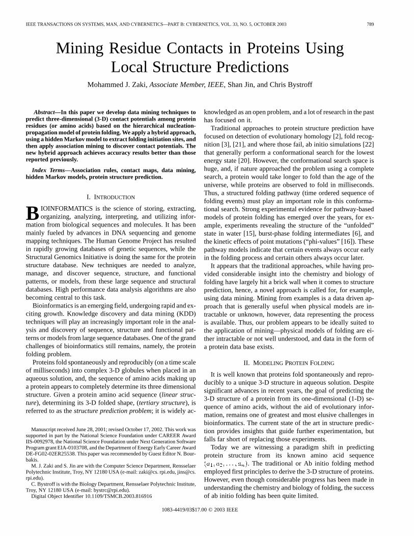
The contact map of a protein (see Fig. 1) is a particularlyuseful representation of protein tertiary structure. Two aminoacids in a protein that come into contact with each other forma noncovalent interaction (hydrogen-bonds, hydrophobic effect,etc.). More formally, we say that two residues (or amino acids)

and in a protein are incontactif the 3-D distanceis less than some threshold value(in this paper we use

as the threshold distance), where , andand are the coordinates of the-carbon atoms of amino

acids and . We definesequence separationas the distancebetween two amino acids and in the amino acid sequence,given as . A contact map for a protein with residues is an

binary matrix whose element if residuesand are in contact, and otherwise. The contact mapprovides a host of useful information. For example, secondarystructure can easily be discerned from it.-Helices appear asthick bands along the main diagonal since they involve contactsbetween one amino acid and its four successors, while-Sheetsare thin bands parallel or anti-parallel to the main diagonal, etc.However, tertiary structure is not easily found from the contact

ZAKI et al.: MINING RESIDUE CONTACTS IN PROTEINS USING LOCAL STRUCTURE PREDICTIONS 791

Fig. 1. Contact map: 3-D structure for protein G (PDB file 2igd,N = 61) and its contact map showing parallel (top left cluster) and anti parallel sheets (bottomleft and top right cluster), and helix features (thin cluster close to main diagonal).

map. For predicting the elusive global fold of a protein we areusually interested in only those contacts that are far from themain diagonal. In this paper we thus, ignore any pair of residueswhose sequence separation .

Previous work on contact prediction has employed neural net-works [8], and statistical techniques based on correlated mu-tations [17], [23]. Recent work by Vendruscoloet al. [24] hasalso shown that it is possible to recover the 3-D structure fromeven corrupted contact maps. In this paper we present a newhybrid technique for contact map prediction. We first predictlocal structural elements using an HMM. The HMM simultane-ously represents the initiation and propagation steps of proteinfolding. We then apply association mining technique on top ofthe HMM states to predict the states that frequently co-occurwith contacts. These sets are then used for predicting contactsin unseen proteins. Our model obtains 19% accuracy and cov-erage over the set of all proteins; the model is also 5.2 timesbetter than a random predictor. We can significantly enhancecoverage to over 40% if we sacrifice accuracy (13%). For shortproteins (length ) we get 30% accuracy and coverage (4.5times better than random); if we lower accuracy to 26% we canget coverage upto 63%. We believe that these results are betterthan (or equal to) those reported previously.

III. H YBRID MINING APPROACH

Here we describe the hybrid technique used in conjunction, topredict residue contacts. We first use an HMM to predict localsubstructures within the protein. We then use meta-level miningon the output of the HMM using association rule mining. TheSections III-A and B provide a brief introduction to these twomethods (readers familiar with them can safely skip ahead).

A. Hidden Markov Models

The description of HMM below is based on the excellent tu-torial by Rabiner [18]. An HMM is a doubly stochastic processwith an underlying stochastic process that is not observable (it

is hidden), but can only be observed through another set of ob-served symbols.

An HMM is made up of a finite number of states. At eachtime step a new state is entered based on a transition probabilitydistribution which depends on the previous state (the Markovianproperty). After each transition is made, an observation outputis produced according to a fixed probability distribution whichdepends on the current state. Thus there asuch observationprobability distributions.

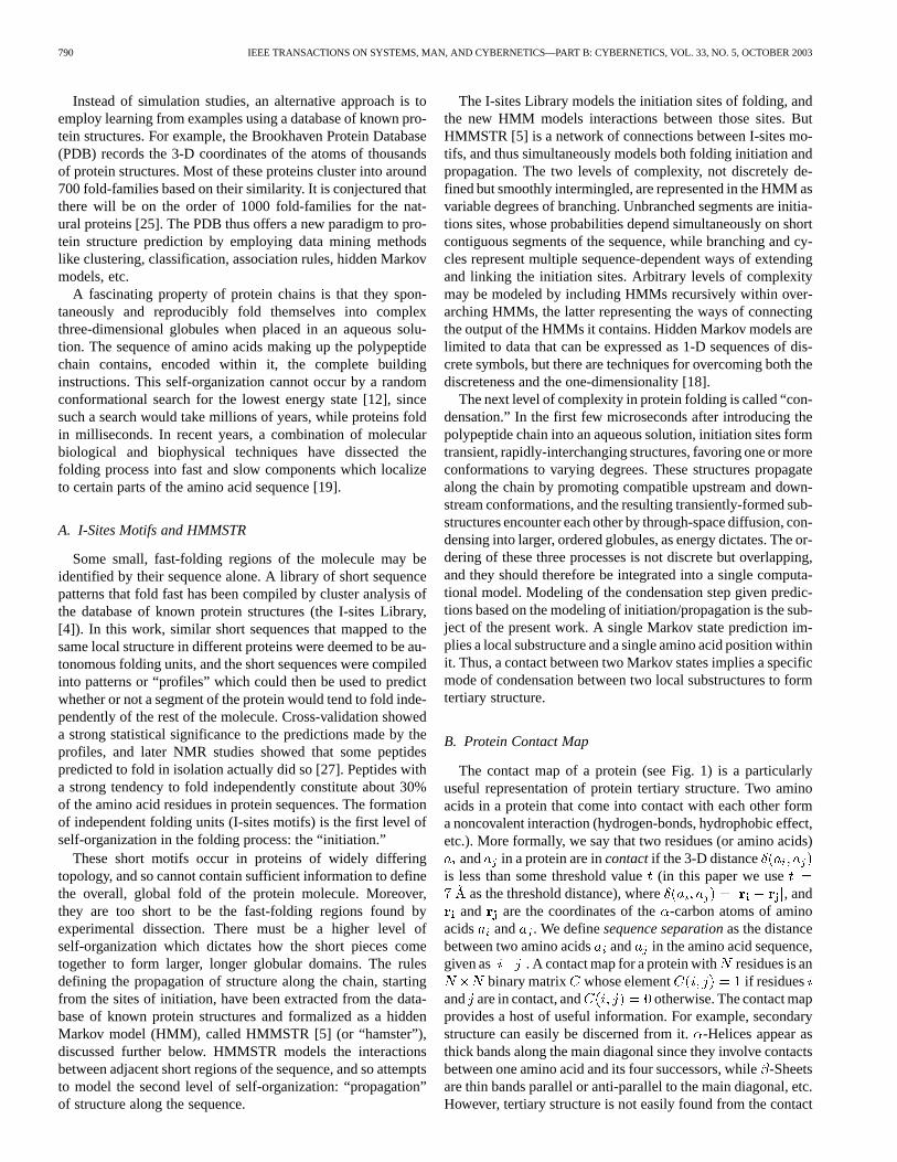
As an example of modeling proteins via HMMs, let con-sider an “urn and residue” model. There areurns (or states)each filled with a large number of the 20 possible amino acids.The observation sequence (a protein?) is generated by initiallychoosing one of the urns (according to an initial probabilitydistribution), selecting a residue from the initial urn, recordingwhich amino acid it is, replacing it, and then choosing a newurn (state) according to a transition probability distribution as-sociated with the current urn. A step corresponds to a residueposition. Thus, a typical observation sequence might look likethis, Table I.

An HMM is made up of the following components: is thelength of the observation sequence;the number of states inthe model; the number of observation symbols (for sim-plicity we assume here that the output is a discrete symbol, e.g.,an amino acid. However we actually use a continuous vectoroutput as we shall see later); is set ofHMM states; is the set of output sym-bols; gives the set of state transition probabilities,i.e., ; is theoutput symbol probability distribution in state, i.e.,

; and finally gives the initial statedistribution, i.e., .

Using the model, an observation sequenceis generated as follows:

1) choose an initial state based on ;2) set position ;3) choose according to ;


TABLE IHYPOTHETICAL STATE AND OBSERVATION FOR AN“URN AND RESIDUE”

MODEL. EACH “URN” CONTAINS A DIFFERENTDISTRIBUTION OFAMINO ACIDS

4) choose according to , ;5) set ; return to step 3 if ; otherwise terminate

the procedure.

An HMM can be compactly represented using the notation. There are three key problems that have to be

solved to build a useful model:

1) Evaluation Problem:Given the observation sequence, and the model , how

to compute the probability of the observed sequence. This can be solved using the Forward-Backward

algorithm [18].2) Estimation Problem:Given the observation sequence

, how to choose a state sequence, which is optimal in some meaningful

sense. This can be solved using the Viterbi algorithm[18].

3) Maximization Problem:How to adjust the model param-eters to maximize . This can besolved using the Baum-Welch reestimation method [18].We will discuss in Section IV the exact details of how theHMM is built to model proteins.

B. Association Rules

Since its introduction, association rule mining (ARM) [1],has become one of the core data mining tasks, and has attractedtremendous interest among data mining researchers and practi-tioners. ARM is an undirected or unsupervised data mining tech-nique, which works on variable length data, and it produces clearand understandable results. It has an elegantly simple problemstatement, that is, to find the set of all subsets of items or at-tributes that frequently occur in many database records or ex-amples, and additionally, to extract the rules telling us how asubset of items influences the presence of another subset.

The association mining task can be stated as follows: Letbe a set of items, and a database of examples, where each ex-ample has a unique identifier (tid) and contains a set of items. Aset of items is also called anitemset. An itemset with itemsis called a -itemset. Thesupportof an itemset , denoted

, is the number of examples in where it occurs asa subset. An itemset isfrequentor large if its support is morethan a user-specifiedminimum support (min_sup)value.

An association ruleis an expression , where andare itemsets. The support of the rule is the joint probability of aexample containing both and , and is given as .The confidenceof the rule is the conditional probability thatan example contains , given that it contains , and is givenas . A rule is frequentif its support is greaterthanmin_sup, and it isstrong if its confidence is more than auser-specifiedminimum confidence (min_conf).

The data mining task is to generate all association rules inthe database, which have a support greater thanmin_sup, i.e.,the rules are frequent, and which also have confidence greaterthanmin_conf, i.e., the rules are strong. In this paper we areinterested in rules with a specific item, called theclass, as aconsequent, i.e., we mine rules of the form where isa class attribute .

This task can be broken into the following two steps:

1) Find all frequent itemsets having minimum support for atleast one class . The search space for enumeration ofall frequent itemsets is , which is exponential in ,the number of items. However, if we assume that there isa bound on the example length, we can show that ARMis essentially linear in the database size [29].

2) Generate strong rules having minimum confidence, fromthe frequent itemsets. We generate and test the confidenceof all rules of the form , where is frequent.

1) Mining Frequent Closed Itemsets:We mine the frequentsets based on the formal concept analysis approach [9], whichis a very elegant mathematical framework for extracting “con-cepts” from databases.

Consider an itemset . Let be the setof all examples in the database where occurs. Furtherlet be the set of all items that arecommon to all examples in the set. Then we say that isclosedif . In other words is the maximal set of itemsthat is common to all examples in. A closed itemset is alsocalled aconcept.

The set of all closed frequent itemsets can be orders of mag-nitude smaller than the set of all frequent itemsets, especiallyfor real (dense) datasets [28]. At the same time, we don’t looseany information; the closed itemsets uniquely determine the setof all frequent itemsets and theirexactfrequency. Thus, insteadof mining all the frequent itemsets we only mine the frequentclosed itemsets using the CHARM algorithm [30] we recentlydeveloped. A detailed description of the algorithm is beyond thescope of this paper. Suffice it to say that CHARM can handlevery large disk-resident or external memory databases; it hasbeen tested on databases with millions of examples, and it scaleslinearly in the database size. We refer the reader to [30] for thealgorithm description and its efficiency.

IV. HMMSTR: AN HMM FOR LOCAL STRUCTURE IN

PROTEINS

We describe here the hidden Markov model, HMMSTR [5],for general protein sequences based on the I-sites library of se-quence-structure motifs [4]. In Section V we will show how weapply association mining on the output of HMMSTR to predictresidue contacts.

Unlike the linear HMMs used to model individual proteinfamilies [7], HMMSTR has a highly branched topology and cap-tures recurrent local features of protein sequences and structuresthat transcend protein family boundaries. The model extendsthe I-sites library by describing the adjacencies of different se-quence-structure motifs as observed in the protein database, and


achieves a great reduction in parameters by representing over-lapping motifs in a much more compact form.

The I-sites (Invariant or Initiation sites) library consists of anextensive set of short sequence motifs, length 3 to 19, obtainedby exhaustive clustering of sequence segments from a nonre-dundant database of known structures [4], [10]. Each sequencepattern correlates strongly with a recurrent local structural motifin proteins. Approximately one third of all residues in the data-base are found in an I-sites motif that can be predicted with ahigh degree of confidence . The library is nonredun-dant in that no motif is completely contained within another,longer motif. However, many of the motifs overlap. Further-more, the isolated motif model does not capture higher orderrelationships such as the distinctly nonrandom transition fre-quencies between the different motifs. The redundancy inherentin the I-sites model suggests a better representation that wouldmodel the diversity of the motifs and their higher order relation-ships while condensing features they have in common. A hiddenMarkov model is well suited to this purpose.

A. Description of HMMSTR

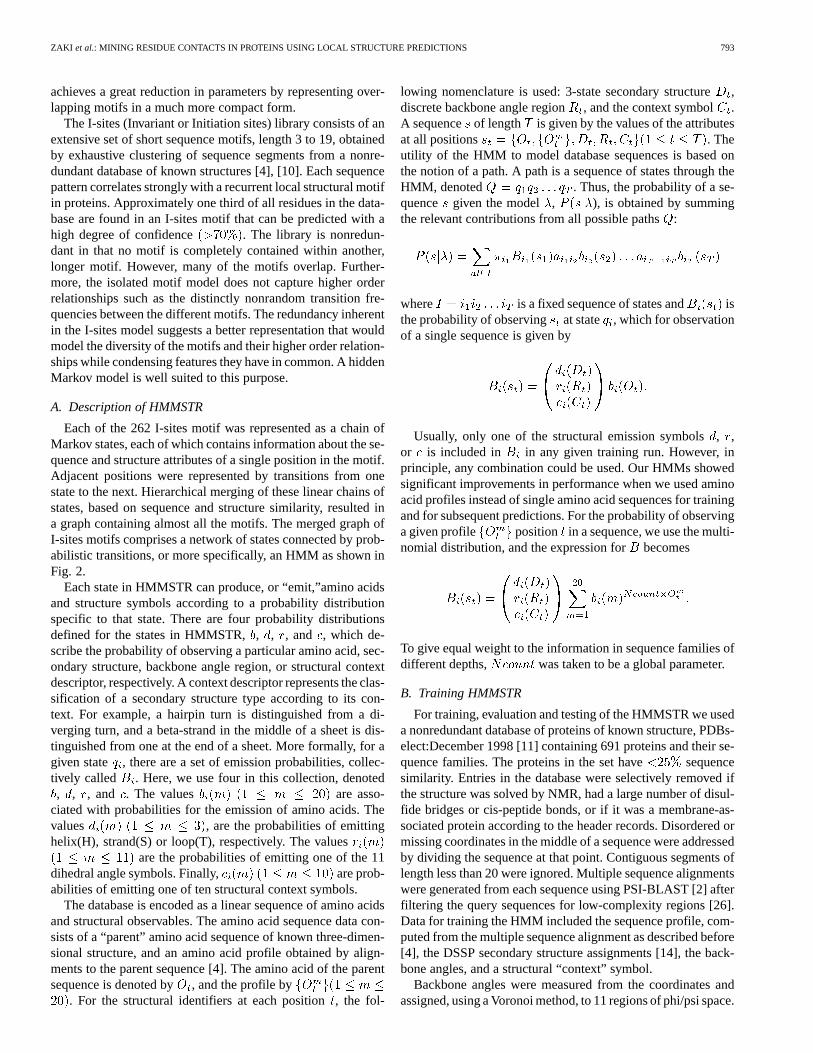
Each of the 262 I-sites motif was represented as a chain ofMarkov states, each of which contains information about the se-quence and structure attributes of a single position in the motif.Adjacent positions were represented by transitions from onestate to the next. Hierarchical merging of these linear chains ofstates, based on sequence and structure similarity, resulted ina graph containing almost all the motifs. The merged graph ofI-sites motifs comprises a network of states connected by prob-abilistic transitions, or more specifically, an HMM as shown inFig. 2.

Each state in HMMSTR can produce, or “emit,”amino acidsand structure symbols according to a probability distributionspecific to that state. There are four probability distributionsdefined for the states in HMMSTR,, , , and , which de-scribe the probability of observing a particular amino acid, sec-ondary structure, backbone angle region, or structural contextdescriptor, respectively. A context descriptor represents the clas-sification of a secondary structure type according to its con-text. For example, a hairpin turn is distinguished from a di-verging turn, and a beta-strand in the middle of a sheet is dis-tinguished from one at the end of a sheet. More formally, for agiven state , there are a set of emission probabilities, collec-tively called . Here, we use four in this collection, denoted, , , and . The values are asso-

ciated with probabilities for the emission of amino acids. Thevalues , are the probabilities of emittinghelix(H), strand(S) or loop(T), respectively. The values

are the probabilities of emitting one of the 11dihedral angle symbols. Finally, are prob-abilities of emitting one of ten structural context symbols.

The database is encoded as a linear sequence of amino acidsand structural observables. The amino acid sequence data con-sists of a “parent” amino acid sequence of known three-dimen-sional structure, and an amino acid profile obtained by align-ments to the parent sequence [4]. The amino acid of the parentsequence is denoted by , and the profile by

. For the structural identifiers at each position, the fol-

lowing nomenclature is used: 3-state secondary structure,discrete backbone angle region, and the context symbol .A sequence of length is given by the values of the attributesat all positions . Theutility of the HMM to model database sequences is based onthe notion of a path. A path is a sequence of states through theHMM, denoted . Thus, the probability of a se-quence given the model , ), is obtained by summingthe relevant contributions from all possible paths:

where is a fixed sequence of states and isthe probability of observing at state , which for observationof a single sequence is given by

Usually, only one of the structural emission symbols, ,or is included in in any given training run. However, inprinciple, any combination could be used. Our HMMs showedsignificant improvements in performance when we used aminoacid profiles instead of single amino acid sequences for trainingand for subsequent predictions. For the probability of observinga given profile position in a sequence, we use the multi-nomial distribution, and the expression forbecomes

To give equal weight to the information in sequence families ofdifferent depths, was taken to be a global parameter.

B. Training HMMSTR

For training, evaluation and testing of the HMMSTR we useda nonredundant database of proteins of known structure, PDBs-elect:December 1998 [11] containing 691 proteins and their se-quence families. The proteins in the set have sequencesimilarity. Entries in the database were selectively removed ifthe structure was solved by NMR, had a large number of disul-fide bridges or cis-peptide bonds, or if it was a membrane-as-sociated protein according to the header records. Disordered ormissing coordinates in the middle of a sequence were addressedby dividing the sequence at that point. Contiguous segments oflength less than 20 were ignored. Multiple sequence alignmentswere generated from each sequence using PSI-BLAST [2] afterfiltering the query sequences for low-complexity regions [26].Data for training the HMM included the sequence profile, com-puted from the multiple sequence alignment as described before[4], the DSSP secondary structure assignments [14], the back-bone angles, and a structural “context” symbol.

Backbone angles were measured from the coordinates andassigned, using a Voronoi method, to 11 regions of phi/psi space.


Fig. 2. HMMSTR model built from I-sites library.

The centroids of ten regions were chosen by K-means clusteringof a large subset of trans phi/psi pairs from the database. The11th region is all cis peptides.

A randomly selected set of 73 of the 691 proteins (19,000positions) was then set aside and not used for training, but onlyfor the final cross-validation. Before cross-validation, a test fortrue independence was applied to each member of the test set,and 12 members were removed. The final test set thus contained61 proteins and 16 000 positions.

The remaining set of 618 parent sequences (145 000 po-sitions) was used for training, and divided into a large set of564 sequences (133 000 positions), used for optimization viathe Expectation-Maximization algorithm, and a small set of 54sequences (12,000 positions) used to evaluate the predictiveability of the model during training. Note that the small set of54 sequences is used only for evaluation of the performanceof a model and may thus appear to be a test set. However,decisions regarding the modification of the model are based


on results of those evaluations. The set of 54 sequences istherefore not a test set, but a training set. For the final round oftraining we re-combined the large and small training sets, to atotal of 618 sequence families. After the final round of training,the models were frozen.

V. DATA FORMAT AND PREPARATION

After HMMSTR is built we again took the 691 proteinsfrom PDBSelect and computed for each protein the optimalHMMSTR states that agree with the observed amino acids inthe protein. In other words for each protein sequence-structurewe solve the estimation problem, i.e., given the observationsequence , how to choose a state sequence

, which is optimal. The output probabilitydistributions of all the states thus chosen for a protein sequenceis used as input for the association mining algorithm. In fact,rather than a single state associated with a given residue,we have available the probability that the residue at thegiven position is associated with all the states of HMMSTR,i.e., we have available for all the 282 HMMSTRstates for all the residues in a given protein( , where is the length of the protein). For eachresidue we also know the amino acid at that position; the, ,, and outputs, which describe the probability of observing

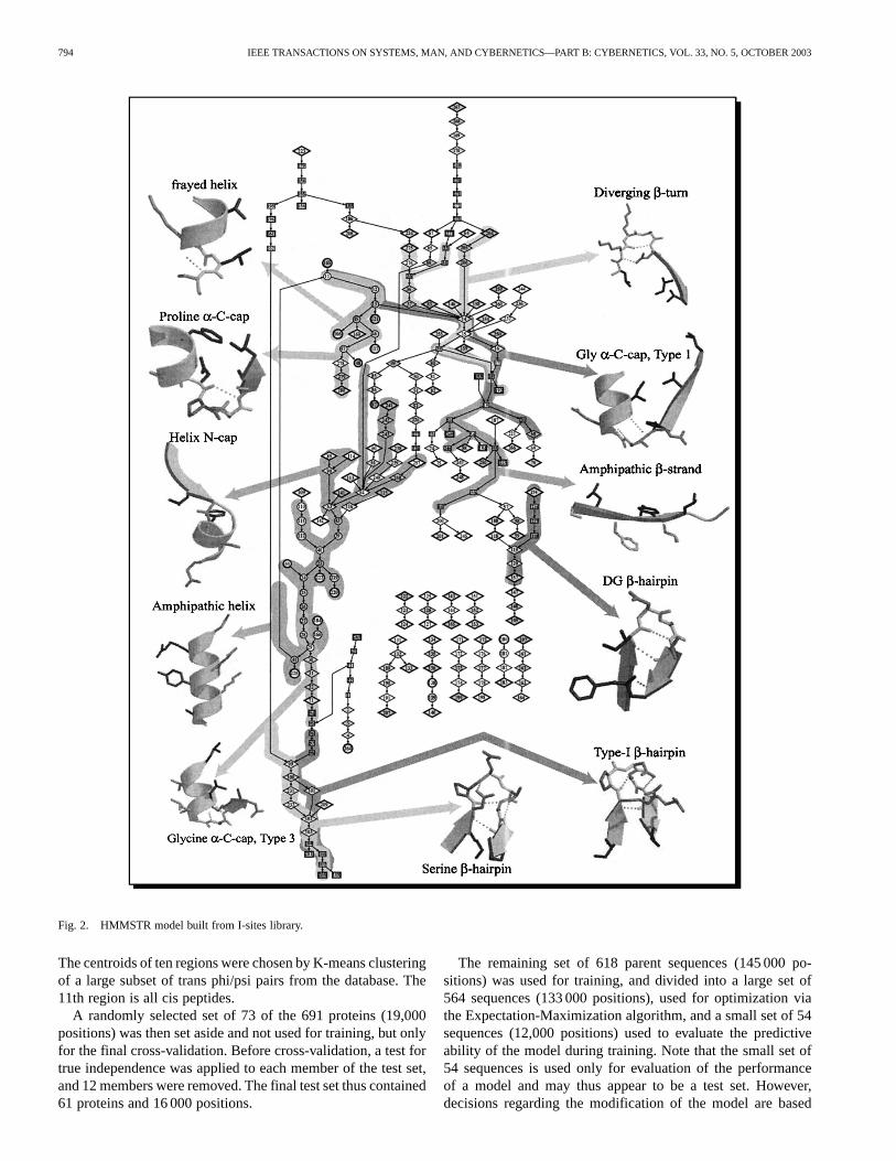
a particular amino acid, secondary structure, backbone angleregion, or structural context descriptor, respectively; the spatialcoordinates of the -Carbon atom ; a distance vectorof length giving the distance of this residue from all otherresidues in the protein; and the 20 amino acid profiles for thatposition. An example protein data file is shown in Fig. 3.

We have a file like the one shown above for all of the 691nonredundant set of proteins from PDBSelect. Disordered ormissing coordinates in the middle of a protein sequence wereaddressed by dividing the sequence at that point. This producesa set of 794 files, most of them containing an entire proteinsequence, but some of these correspond to proteins that weresplit.

Given a protein file, we now have to transform the data into aformat that can be easily mined for frequent closed itemsets,i.e., we need to prepare the data in the relational or tabularformat where we have multiple attributes (columns) for eachexample (rows) or record. Since we are interested in predictingthe contact between a pair of amino acids, we use each pair asan example in the training set, associated with a specialclassattribute indicating whether it is a contact or noncontact

; amino acids and are in contact if ,i.e., the distance between-carbons of amino acids and isless then 7 . Our new database has an entry showing the twoamino acids and their class for each pair of amino acids for eachprotein. In order to avoid predicting purely local contacts we ig-nore all pairs whose sequence separation . Note alsothat the number of contacts is a lot smaller than the numberof noncontacts for any protein.

We found that the percentage of contacts (or number of data-base entries with class 1) over all pairs is less than 1.7%. Across

Fig. 3. Example of a protein data file.

the 794 files, the longest sequence had length 907, while thesmallest had length 35. There were 17 618 115 pairs over allproteins, while only 292 126 pairs were in contact. This data-base thus corresponds to a highly biased binary classificationproblem. That is, we have to build a mining model that candiscriminate between contacts and noncontacts between aminoacids pairs, where the examples are overwhelmingly biased to-ward the noncontacts.

Our database so far doesn’t have enough information for gooddiscrimination. All we have is the amino acids making up thepair and whether they are in contact or not. We need to addmore “context” information to facilitate the classification. It iseasy to incorporate, for each amino acid in the pair, the 3 sec-ondary structure symbols , the 11 backbone angle re-gions , and the 10 structural context descriptors .For each pair we would also like to add the HMMSTR stateprobabilities. Since association rules only work for categoricalattributes, we need to convert the continuous state probabilitiesinto discrete values. To do this we take the ratio of each of the282 HMMSTR state probabilities for against the backgroundor prior probability of an amino acid being in that state; if theratio is more than some threshold we include the state in thecontext of , else we ignore it. We repeat the same process for

. Using a similar thresholding method one can incorporate theamino acid profiles for positionsand . With all this contextinformation for both and we obtain a new database to beused to find the frequent itemsets characterizing the contacts and


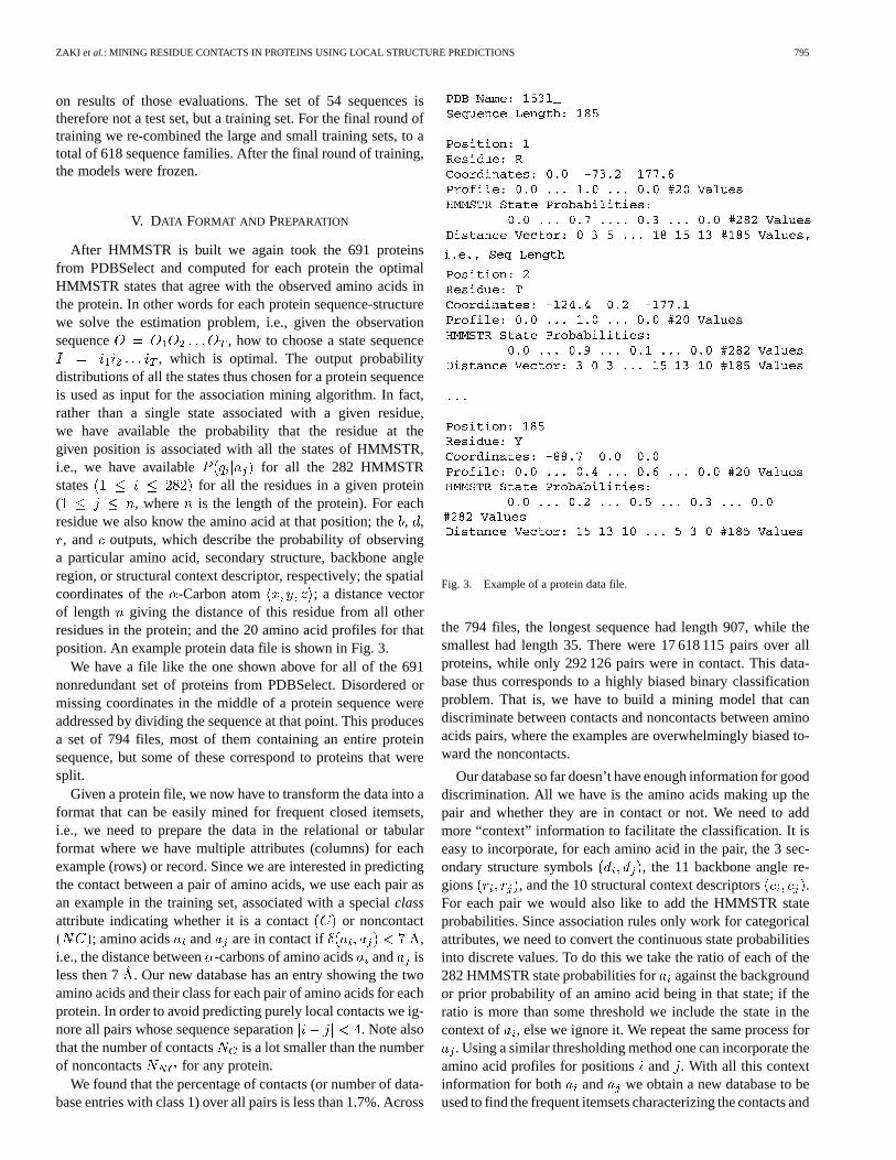
noncontacts. In summary the database might have the followingcolumns for pairs of amino acids over all proteins.

Note that the number of columns can be variable for differentpairs depending on the profile and HMMSTR state probabilities.

, , etc. show the other amino acids that can appear in po-sition (provided the probability is more than some threshold),and finally , , etc. show HMMSTR states with probabil-ities more than some factor of the prior probability of thosestates.

VI. A SSOCIATIONMINING ON THE PAIRS DATABASE

We are now in a position to cast the above database in theassociation framework. Each attribute-value pair is an item, andis represented with a fixed, unique integer. For exampleis one item and is another item. By the same tokeneach value of , , , , and is a different item. Each ofthe HMMSTR states becomes a distinct item, as do the profilevalues. The items for the context attributes ofand are alsokept distinct. Finally we separate the examples that are contactsfrom those that are noncontacts to get two databases, denoted as

and , respectively.Given these databases our goal is to find high support and

high confidence rules of the form and , thatdiscriminate between the contact pairs and the noncontact pairs,respectively. Below we describe the mining/training and testingphases, where we learn from examples using the frequent closeditemsets, and then classify unseen examples as being contacts ornoncontacts, respectively.

A. Mining on Known Examples

The goal of the mining phase is to learn from known contactand noncontact examples and build a model or rule set that dis-criminates between the two classes. We selected a random 90%of the files for training, out of a total of 794 files. The remaining10% of the files were kept aside for testing the mined rule set.

Since we are primarily interested in predicting the contactsrather than the noncontacts, we mine only on the contacts data-base . However, we do use the noncontacts database toprune out those itemsets that are frequent in both sets. Buildinga discriminative rule set consists of the following steps, in order:

1) Mining: We use CHARM [30] to mine all the frequentclosed itemsets in based on a suitably chosen min_supvalue. Let’s denote the set of frequent closed itemsets as

.2) Counting: We compute the support of all itemsets inin

the noncontacts database .

3) Pruning: We compute the probability of occurrence ofeach itemset in in both the contact and noncontactdatabases. The probability of occurrence is simply thesupport of the itemset divided by the number of exam-ples in the given dataset. For example, if itemset ,then the probability of its occurrence in is given as

.

As a first step in pruning we can remove all itemsetswhich have a greater probability of occurrence in the noncon-tact database than in the contact database, i.e., if

. Actually, we compute the ratio of the contact proba-bility versus the noncontact probability for, and prune it if thisratio is less than some suitably chosen threshold, i.e., we prune

if . In other words we want toretain only those itemset that have a much greater chance of pre-dicting a contact rather than a noncontact.

B. Testing on Unknown Examples

The goal of the testing phase is to find how accurately themined set of rules predict the contacts versus the noncontactsin new examples not used for training. We used a random 10%of the files in the database for testing. The test set had a total oftwo 336 548 pairs, out of which 35 987 or 1.54% were contacts.Since we do know the true class of each example it is easy forus to find out how well our rules are for prediction.

For testing we generate a combined databasecontainingall pairs of amino acids in contact or otherwise. For each ex-ample we know the true class. We assign each example a pre-dicted class using the following steps:

1) Evidence CalculationFor each example in the testdataset , we compute which itemsets in the set of minedand pruned closed frequent itemsetsare subsets of .Let’s denote the set of these itemsets as. We next cal-culate the cumulative contact and noncontact support forexample , i.e., the sum of the supports of all itemsetsin in the contact and noncontact database. Finally, wecompute the evidence for being a contact, i.e., we takethe ratio of the cumulative contact support over cumula-tive noncontact support, denoted as. Any examplewith zero contact support is taken to be a noncontact anddiscarded, and only the examples or test pairs with posi-tive contact support are retained for the next step.

2) PredictionTo make the final prediction if a test pair ofresidues is in contact or not, we sort all test examples(with positive cumulative contact support) in decreasingorder of contact evidence . Finally, the top fraction ofexamples in terms of are predicted to be contacts andthe remaining fraction of examples as noncontacts.How is chosen will be explained below.

C. Model Accuracy and Coverage

In predicting contacts versus noncontacts for the test exam-ples, we have to evaluate the mined model based on two metrics:AccuracyandCoverage. Furthermore, we are only interested inthe prediction of contacts; thus accuracy and coverage is onlyconsidered for contacts. Accuracy is the ratio of correct con-tacts to the predicted contacts, while coverage is the percentage


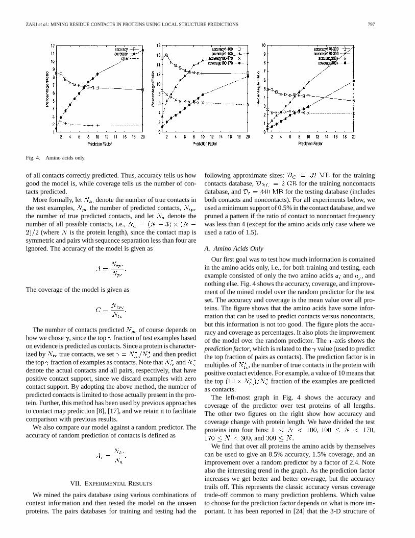
Fig. 4. Amino acids only.

of all contacts correctly predicted. Thus, accuracy tells us howgood the model is, while coverage tells us the number of con-tacts predicted.

More formally, let denote the number of true contacts inthe test examples, the number of predicted contacts,the number of true predicted contacts, and let denote thenumber of all possible contacts, i.e.,

(where is the protein length), since the contact map issymmetric and pairs with sequence separation less than four areignored. The accuracy of the model is given as

The coverage of the model is given as

The number of contacts predicted of course depends onhow we chose , since the top fraction of test examples basedon evidence is predicted as contacts. Since a protein is character-ized by true contacts, we set and then predictthe top fraction of examples as contacts. Note that anddenote the actual contacts and all pairs, respectively, that havepositive contact support, since we discard examples with zerocontact support. By adopting the above method, the number ofpredicted contacts is limited to those actually present in the pro-tein. Further, this method has been used by previous approachesto contact map prediction [8], [17], and we retain it to facilitatecomparison with previous results.

We also compare our model against a random predictor. Theaccuracy of random prediction of contacts is defined as

VII. EXPERIMENTAL RESULTS

We mined the pairs database using various combinations ofcontext information and then tested the model on the unseenproteins. The pairs databases for training and testing had the

following approximate sizes: for the trainingcontacts database, for the training noncontactsdatabase, and for the testing database (includesboth contacts and noncontacts). For all experiments below, weused a minimum support of 0.5% in the contact database, and wepruned a pattern if the ratio of contact to noncontact frequencywas less than 4 (except for the amino acids only case where weused a ratio of 1.5).

A. Amino Acids Only

Our first goal was to test how much information is containedin the amino acids only, i.e., for both training and testing, eachexample consisted of only the two amino acidsand , andnothing else. Fig. 4 shows the accuracy, coverage, and improve-ment of the mined model over the random predictor for the testset. The accuracy and coverage is the mean value over all pro-teins. The figure shows that the amino acids have some infor-mation that can be used to predict contacts versus noncontacts,but this information is not too good. The figure plots the accu-racy and coverage as percentages. It also plots the improvementof the model over the random predictor. The-axis shows theprediction factor, which is related to the value (used to predictthe top fraction of pairs as contacts). The prediction factor is inmultiples of , the number of true contacts in the protein withpositive contact evidence. For example, a value of 10 means thatthe top fraction of the examples are predictedas contacts.

The left-most graph in Fig. 4 shows the accuracy andcoverage of the predictor over test proteins of all lengths.The other two figures on the right show how accuracy andcoverage change with protein length. We have divided the testproteins into four bins: , ,

, and .We find that over all proteins the amino acids by themselves

can be used to give an 8.5% accuracy, 1.5% coverage, and animprovement over a random predictor by a factor of 2.4. Notealso the interesting trend in the graph. As the prediction factorincreases we get better and better coverage, but the accuracytrails off. This represents the classic accuracy versus coveragetrade-off common to many prediction problems. Which valueto choose for the prediction factor depends on what is more im-portant. It has been reported in [24] that the 3-D structure of


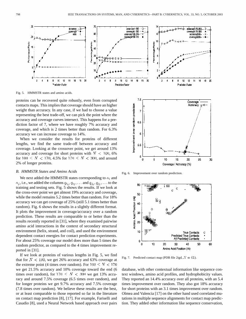
Fig. 5. HMMSTR states and amino acids.

proteins can be recovered quite robustly, even from corruptedcontacts maps. This implies that coverage should have an higherweight than accuracy. In any case, if we had to choose a valuerepresenting the best trade-off, we can pick the point where theaccuracy and coverage curves intersect. This happens for a pre-diction factor of 7, where we have roughly 7% accuracy andcoverage, and which is 2 times better than random. For 6.3%accuracy we can increase coverage to 14%.

When we consider the results for proteins of differentlengths, we find the same trade-off between accuracy andcoverage. Looking at the crossover point, we get around 13%accuracy and coverage for short proteins with , 6%for , 4.5% for , and around2% of longer proteins.

B. HMMSTR States and Amino Acids

We next added the HMMSTR states corresponding toand, i.e., we added the columns and to the

training and testing sets. Fig. 5 shows the results. If we look atthe cross-over point we get almost 19% accuracy and coverage,while the model remains 5.2 times better than random. For 18%accuracy we can get coverage of 25% (still 5.1 times better thanrandom). Fig. 6 shows the results in a slightly different format.It plots the improvement in coverage/accuracy over a randomprediction. These results are comparable to or better than theresults recently reported in [31], where they examined pairwiseamino acid interactions in the context of secondary structuralenvironment (helix, strand, and coil), and used the environmentdependent contact energies for contact prediction experiments.For about 25% coverage our model does more than 5 times therandom predictor, as compared to the 4 times improvement re-ported in [31].

If we look at proteins of various lengths in Fig. 5, we findthat for , we get 26% accuracy and 63% coverage atthe extreme point (4 times over random). Forwe get 21.5% accuracy and 10% coverage toward the end (6times over random), for we get 13% accu-racy and around 7.5% coverage (6.5 times over random), andfor longer proteins we get 9.7% accuracy and 7.5% coverage(7.8 times over random). We believe these results are the best,or at least comparable to those reported so far in the literatureon contact map prediction [8], [17]. For example, Fariselli andCasadio [8], used a Neural Network based approach over pairs

Fig. 6. Improvement over random prediction.

Fig. 7. Predicted contact map (PDB file 2igd,N = 61).

database, with other contextual information like sequence con-text windows, amino acid profiles, and hydrophobicity values.They reported an 14.4% accuracy over all proteins, with an 5.4times improvement over random. They also got 18% accuracyfor short proteins with an 3.1 times improvement over random.Olmea and Valencia [17] on the other hand used correlated mu-tations in multiple sequence alignments for contact map predic-tion. They added other information like sequence conservation,


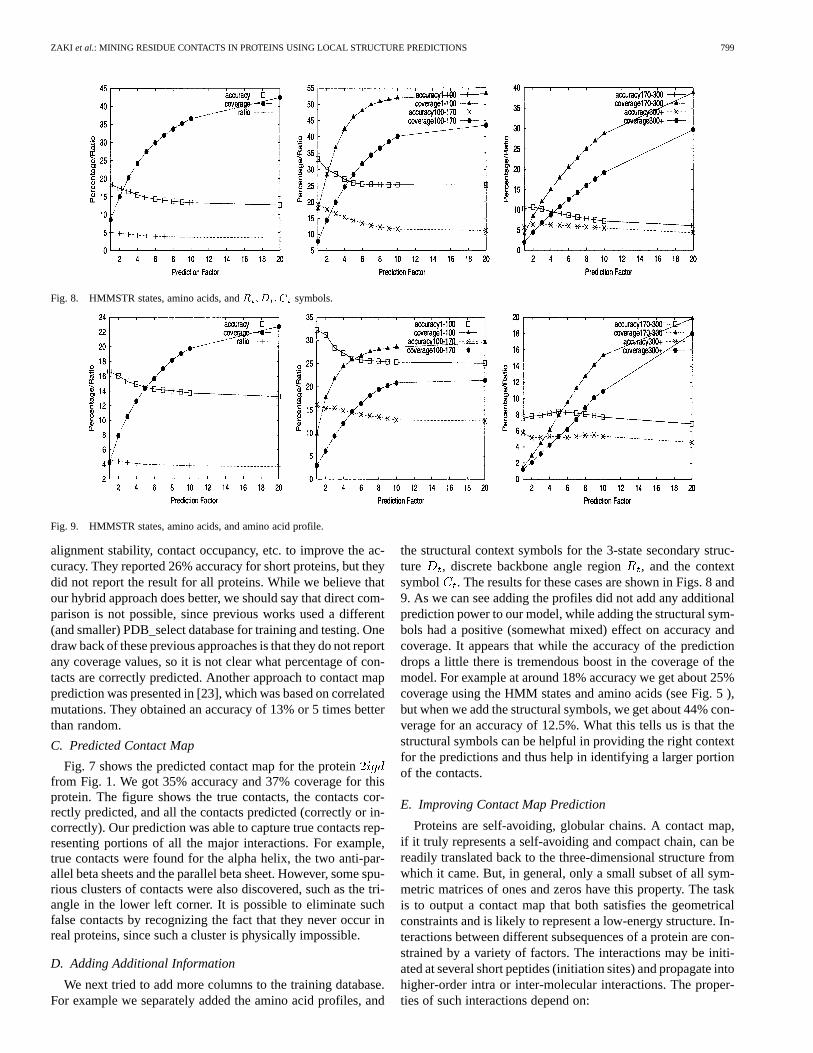
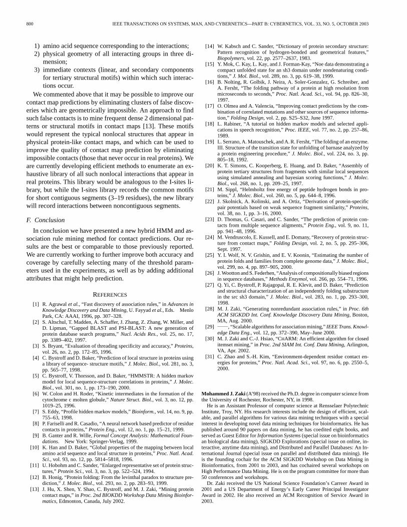
Fig. 8. HMMSTR states, amino acids, andR ;D ;C symbols.

Fig. 9. HMMSTR states, amino acids, and amino acid profile.

alignment stability, contact occupancy, etc. to improve the ac-curacy. They reported 26% accuracy for short proteins, but theydid not report the result for all proteins. While we believe thatour hybrid approach does better, we should say that direct com-parison is not possible, since previous works used a different(and smaller) PDB_select database for training and testing. Onedraw back of these previous approaches is that they do not reportany coverage values, so it is not clear what percentage of con-tacts are correctly predicted. Another approach to contact mapprediction was presented in [23], which was based on correlatedmutations. They obtained an accuracy of 13% or 5 times betterthan random.

C. Predicted Contact Map

Fig. 7 shows the predicted contact map for the proteinfrom Fig. 1. We got 35% accuracy and 37% coverage for thisprotein. The figure shows the true contacts, the contacts cor-rectly predicted, and all the contacts predicted (correctly or in-correctly). Our prediction was able to capture true contacts rep-resenting portions of all the major interactions. For example,true contacts were found for the alpha helix, the two anti-par-allel beta sheets and the parallel beta sheet. However, some spu-rious clusters of contacts were also discovered, such as the tri-angle in the lower left corner. It is possible to eliminate suchfalse contacts by recognizing the fact that they never occur inreal proteins, since such a cluster is physically impossible.

D. Adding Additional Information

We next tried to add more columns to the training database.For example we separately added the amino acid profiles, and

the structural context symbols for the 3-state secondary struc-ture , discrete backbone angle region, and the contextsymbol . The results for these cases are shown in Figs. 8 and9. As we can see adding the profiles did not add any additionalprediction power to our model, while adding the structural sym-bols had a positive (somewhat mixed) effect on accuracy andcoverage. It appears that while the accuracy of the predictiondrops a little there is tremendous boost in the coverage of themodel. For example at around 18% accuracy we get about 25%coverage using the HMM states and amino acids (see Fig. 5 ),but when we add the structural symbols, we get about 44% con-verage for an accuracy of 12.5%. What this tells us is that thestructural symbols can be helpful in providing the right contextfor the predictions and thus help in identifying a larger portionof the contacts.

E. Improving Contact Map Prediction

Proteins are self-avoiding, globular chains. A contact map,if it truly represents a self-avoiding and compact chain, can bereadily translated back to the three-dimensional structure fromwhich it came. But, in general, only a small subset of all sym-metric matrices of ones and zeros have this property. The taskis to output a contact map that both satisfies the geometricalconstraints and is likely to represent a low-energy structure. In-teractions between different subsequences of a protein are con-strained by a variety of factors. The interactions may be initi-ated at several short peptides (initiation sites) and propagate intohigher-order intra or inter-molecular interactions. The proper-ties of such interactions depend on:


1) amino acid sequence corresponding to the interactions;2) physical geometry of all interacting groups in three di-

mension;3) immediate contexts (linear, and secondary components

for tertiary structural motifs) within which such interac-tions occur.

We commented above that it may be possible to improve ourcontact map predictions by eliminating clusters of false discov-eries which are geometrically impossible. An approach to findsuch false contacts is to mine frequent dense 2 dimensional pat-terns or structural motifs in contact maps [13]. These motifswould represent the typical nonlocal structures that appear inphysical protein-like contact maps, and which can be used toimprove the quality of contact map prediction by eliminatingimpossible contacts (those that never occur in real proteins). Weare currently developing efficient methods to enumerate an ex-haustive library of all such nonlocal interactions that appear inreal proteins. This library would be analogous to the I-sites li-brary, but while the I-sites library records the common motifsfor short contiguous segments (3–19 residues), the new librarywill record interactions between noncontiguous segments.

F. Conclusion

In conclusion we have presented a new hybrid HMM and as-sociation rule mining method for contact predictions. Our re-sults are the best or comparable to those previously reported.We are currently working to further improve both accuracy andcoverage by carefully selecting many of the threshold param-eters used in the experiments, as well as by adding additionalattributes that might help prediction.

REFERENCES

[1] R. Agrawalet al., “Fast discovery of association rules,” inAdvances inKnowledge Discovery and Data Mining, U. Fayyadet al., Eds. MenloPark, CA: AAAI, 1996, pp. 307–328.

[2] S. Altschul, T. Madden, A. Schaffer, J. Zhang, Z. Zhang, W. Miller, andD. Lipman, “Gapped BLAST and PSI-BLAST: A new generation ofprotein database search programs,”Nucl. Acids Res., vol. 25, no. 17,pp. 3389–402, 1997.

[3] S. Bryant, “Evaluation of threading specificity and accuracy,”Proteins,vol. 26, no. 2, pp. 172–85, 1996.

[4] C. Bystroff and D. Baker, “Prediction of local structure in proteins usinga library of sequence- structure motifs,”J. Molec. Biol., vol. 281, no. 3,pp. 565–77, 1998.

[5] C. Bystroff, V. Thorsson, and D. Baker, “HMMSTR: A hidden markovmodel for local sequence-structure correlations in proteins,”J. Molec.Biol., vol. 301, no. 1, pp. 173–190, 2000.

[6] W. Colon and H. Roder, “Kinetic intermediates in the formation of thecytochrome c molten globule,”Nature Struct. Biol., vol. 3, no. 12, pp.1019–25, 1996.

[7] S. Eddy, “Profile hidden markov models,”Bioinform., vol. 14, no. 9, pp.755–63, 1998.

[8] P. Fariselli and R. Casadio, “A neural network based predictor of residuecontacts in proteins,”Protein Eng., vol. 12, no. 1, pp. 15–21, 1999.

[9] B. Ganter and R. Wille,Formal Concept Analysis: Mathematical Foun-dations. New York: Springer-Verlag, 1999.

[10] K. Han and D. Baker, “Global properties of the mapping between localamino acid sequence and local structure in proteins,”Proc. Natl. Acad.Sci., vol. 93, no. 12, pp. 5814–5818, 1996.

[11] U. Hobohm and C. Sander, “Enlarged representative set of protein struc-tures,”Protein Sci., vol. 3, no. 3, pp. 522–524, 1994.

[12] B. Honig, “Protein folding: From the levinthal paradox to structure pre-diction,” J. Molec. Biol., vol. 293, no. 2, pp. 283–93, 1999.

[13] J. Hu, X. Shen, Y. Shao, C. Bystroff, and M. J. Zaki, “Mining proteincontact maps,” inProc. 2nd BIOKDD Workshop Data Mining Bioinfor-matics, Edmonton, Canada, July 2002.

[14] W. Kabsch and C. Sander, “Dictionary of protein secondary structure:Pattern recognition of hydrogen-bonded and geometrical features,”Biopolymers, vol. 22, pp. 2577–2637, 1983.

[15] Y. Mok, C. Kay, L. Kay, and J. Forman-Kay, “Noe data demonstrating acompact unfolded state for an sh3 domain under nondenaturing condi-tions,” J. Mol. Biol., vol. 289, no. 3, pp. 619–38, 1999.

[16] B. Nolting, R. Golbik, J. Neira, A. Soler-Gonzalez, G. Schreiber, andA. Fersht, “The folding pathway of a protein at high resolution frommicroseconds to seconds,”Proc. Natl. Acad. Sci., vol. 94, pp. 826–30,1997.

[17] O. Olmea and A. Valencia, “Improving contact predictions by the com-bination of correlated mutations and other sources of sequence informa-tion,” Folding Design, vol. 2, pp. S25–S32, June 1997.

[18] L. Rabiner, “A tutorial on hidden markov models and selected appli-cations in speech recognition,”Proc. IEEE, vol. 77, no. 2, pp. 257–86,1989.

[19] L. Serrano, A. Matouschek, and A. R. Fersht, “The folding of an enzyme.III. Structure of the transition state for unfolding of barnase analyzed bya protein engineering procedure,”J. Molec. Biol., vol. 224, no. 3, pp.805–18, 1992.

[20] K. T. Simons, C. Kooperberg, E. Huang, and D. Baker, “Assembly ofprotein tertiary structures from fragments with similar local sequencesusing simulated annealing and bayesian scoring functions,”J. Molec.Biol., vol. 268, no. 1, pp. 209–25, 1997.

[21] M. Sippl, “Helmholtz free energy of peptide hydrogen bonds in pro-teins,”J. Molec. Biol., vol. 260, no. 5, pp. 644–8, 1996.

[22] J. Skolnick, A. Kolinski, and A. Ortiz, “Derivation of protein-specificpair potentials based on weak sequence fragment similarity,”Proteins,vol. 38, no. 1, pp. 3–16, 2000.

[23] D. Thomas, G. Casari, and C. Sander, “The prediction of protein con-tacts from multiple sequence aligments,”Protein Eng., vol. 9, no. 11,pp. 941–48, 1996.

[24] M. Vendruscolo, E. Kussell, and E. Domany, “Recovery of protein struc-ture from contact maps,”Folding Design, vol. 2, no. 5, pp. 295–306,Sept. 1997.

[25] Y. I. Wolf, N. V. Grishin, and E. V. Koonin, “Estimating the number ofprotein folds and families from complete genome data,”J. Molec. Biol.,vol. 299, no. 4, pp. 897–905, 2000.

[26] J. Wootton and S. Federhen, “Analysis of compositionally biased regionsin sequence databases,”Methods Enzymol, vol. 266, pp. 554–71, 1996.

[27] Q. Yi, C. Bystroff, P. Rajagopal, R. E. Klevit, and D. Baker, “Predictionand structural characterization of an independently folding substructurein the src sh3 domain,”J. Molec. Biol., vol. 283, no. 1, pp. 293–300,1998.

[28] M. J. Zaki, “Generating nonredundant association rules,” inProc. 6thACM SIGKDD Int. Conf. Knowledge Discovery Data Mining, Boston,MA, Aug. 2000.

[29] , “Scalable algorithms for association mining,”IEEE Trans. Knowl-edge Data Eng., vol. 12, pp. 372–390, May–June 2000.

[30] M. J. Zaki and C.-J. Hsiao, “CHARM: An efficient algorithm for closeditemset mining,” inProc. 2nd SIAM Int. Conf. Data Mining, Arlington,VA, Apr. 2002.

[31] C. Zhao and S.-H. Kim, “Environment-dependent residue contact en-ergies for proteins,”Proc. Natl. Acad. Sci., vol. 97, no. 6, pp. 2550–5,2000.

Mohammed J. Zaki (A’98) received the Ph.D. degree in computer science fromthe University of Rochester, Rochester, NY, in 1998.

He is an Assistant Professor of computer science at Rensselaer PolytechnicInstitute, Troy, NY. His research interests include the design of efficient, scal-able, and parallel algorithms for various data mining techniques with a specialinterest in developing novel data mining techniques for bioinformatics. He haspublished around 90 papers on data mining, he has coedited eight books, andserved as Guest Editor forInformation Systems(special issue on bioinformaticsan biological data mining), SIGKDD Explorations (special issue on online, in-teractive, anytime data mining), and Distributed and Parallel Databases: An In-ternational Journal (special issue on parallel and distributed data mining). Heis the founding cochair for the ACM SIGKDD Workshop on Data Mining inBioinformatics, from 2001 to 2003, and has cochaired several workshops onHigh Performance Data Mining. He is on the program committee for more than50 conferences and workshops.

Dr. Zaki received the US National Science Foundation’s Carreer Award in2001 and a US Department of Energy’s Early Career Principal InvestigatorAward in 2002. He also received an ACM Recognition of Service Award in2003.


Shan Jin received the M.S. degree in computer science from Rensselaer Poly-technic Institute, Troy, NY in 2001.

Chris Bystroff received the Ph.D. degree from the University of California, SanDiego, in 1988.

He is an Assistant Professor of biology at Rensselaer Polytechnic Institute(RPI), Troy, NY. Before joining RPI in 1999, he worked with J. Kraut, R. Fiett-erick, and D. Baker and taught as a Fullbright Fellow to Nicaragua. He has pub-lished numerous articles on protein crystallography and bioinformatrics, withspecial regard to protein folding. He was a co-organizer of the ChautauquaSummer Workshop in Bioinformatics in 2001, and was a Guest Editor for aspecial issue in theScientific Programming Journal on Hidden Markov Models.

mining residue contacts in proteins using local structure ...zaki/paperdir/tsmc03.pdf · ieee...

Documents