minimum temperature surveys based on near-surface air temperature measurements and airborne thermal...

JOURNAL OF CLIMATOLOGY, VOL. 6, 413-430 (1986) 551.524.36(944):551.509.323.2

MINIMUM TEMPERATURE SURVEYS BASED ON

AIRBORNE THERMAL SCANNER DATA NEAR-SURFACE AIR TEMPERATURE MEASUREMENTS AND

J. D. KALMA Division of Water and Land Resources, Institute of Biological Resources, CSIRO, Canberra City, A . C. T., Australia

G. P. LAUGHLIN School of Geography, University of New South Wales, Kensington, N.S. W . , Australia

AND A. A . GREEN AND M. T. O’BRIEN

Division of Mineral Physics, Institute of Energy and Earth Resources, CSIRO, North Ryde, N. S . W . , Australia

Received 27 March 1985 Revised 16 October 1985

ABSTRACT Minimum air temperature measurements and airborne thermal scanner measurements of apparent surface temperature were obtained in a regional frost risk study in gently undulating grazing country in the Southern Tablelands of New South Wales, Australia.

The minimum air temperature data obtained at 7 sites on 100 nights have been used to derive a predictive relationship between temperature lapse rate and night-time wind speed and net radiation loss. An extended network was used on 30 nights using an additional 24 sites. Excellent agreement was observed between the lapse rates collected from both the 7-station and 31-station networks on 24 nights.

Maps of minimum air temperature across the region have been obtained for selected individual nights using Laplacian smoothing spline functions based on elevation and map co-ordinates.

Thermal scanner data were obtained with an aircraft on two nights and the paper presents detailed comparisons between apparent surface temperature data and minimum air temperatures obtained from the regional maps.

These comparisons have made it possible to successfully distinguish between broad topographic controls and the effect of local surface characteristics, especially in the case of high-resolution thermal scanner data. Such local controls include the effects of trees, surface water and various man-made features, as well as very local topographic features such as narrow depressions, which are only noticeable from site surveys and detailed aerial photography. It is concluded that thermal imagery is an important aid in understanding spatial distribution patterns of night-time air temperatures and hence in regional frost risk assessment.

KEY WORDS Topoclimate Frost Airborne thermal scanner Temperature surveys

INTRODUCTION

Regional surveys of minimum air temperature are traditionally based on costly networks of measuring sites or mobile topoclimatological surveys. However, especially in complex terrain, the network density is seldom adequate for developing local frost risk maps and mobile surveys may not be feasible. Also, objective mapping techniques have rarely been used.

Relatively simple methods must therefore be developed for assessing local frost hazard and for the local interpretation of regional short-term frost warnings (Bagdonas et al., 1978). The use of temperature averages tends to mask differences between nights and it is important to consider rational ways of incorporating such differences in temperature assessment and prediction methods.

0196- 1748/86/040413- 18$09.00 0 1986 by the Royal Meteorological Society

414 J. D. KALMA ET AL.

The use of thermal imagery from satellites in climatology has been discussed by Chen et al. (1979, 1982, 1983) and Byrne et al. (1984). Chen et al. (1983) noted the agreement between surface temperatures observed with the SMS/GOES satellite and 1-5 m air temperatures measured in standard screens and in mobile surveys. Each pixel of the low resolution GOES infra-red imagery represents an area of about 48 km'.

Satisfactory agreement between the HCMM satellite measurements of apparent surface temperatures and (near) surface temperatures measured on the ground was reported by Caselles et al. (1983) and Byrne et al. (1984). Kalma et al. (1983) used Heat Capacity Mapping Mission satellite night-time thermal imagery in a detailed frost risk assessment in Southern Victoria. They observed good agreement with risk maps based on terrain and land cover and noted that the spatial resolution of the HCMM system (pixel area 0.36 km2) was insufficient for local frost mapping.

The use of aircraft-based thermal infra-red imagery in local frost studies is described by Nixon and Hales (1975) and Endlicher (1980). However, relatively few studies have reported on the use of thermal scanners in aircraft for regional climate studies and on comparisons between scanner data and ground-based measurements. The major drawback has been the lack of suitable ground data. For example Mahrt and Heald (1983) recently reported on the close link between apparent surface temperature and terrain curvature, yet provided no comparison between scanner and ground data. Note that the spatial resolution for thermal scanners in aircraft ranges between 1 and 20m, thus yielding a pixel area of between 0-00001 and 0-0004 km'.

The present paper, which consists of two parts, is concerned with developing new techniques for local frost surveys. The study is based on near-surface temperature measurements with a dense network of measuring sites during 30 nights, as well as on thermal imagery obtained on two nights. The objectives of the first part of this study were (i) to assess the role of elevation as the most important determinant of minimum temperature variation in the region, (ii) to identify the effect of weather conditions on the temperature lapse rate and (iii) to produce computer-generated maps of minimum air temperature based on Laplacian smoothing spline functions of elevation and map co-ordinates (i.e. position). The objectives of the second part of this study were to obtain on selected nights high level and low level thermal imagery with an airborne thermal scanner and to compare it with detailed computer-generated regional maps of minimum air temperature, based on temperature measurements made during those nights. However, this study is not concerned with developing predictive equations for use in frost studies elsewhere.

THE STUDY AREA

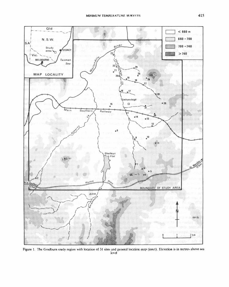
The study area is in the Southern Tablelands of New South Wales, some 160 km south-west of Sydney (see Figure 1). Elevations vary between 600 and 900 m above mean sea level.

Most of the area consists of open and undulating terrain and is used for grazing. The vegetation is dominated by introduced and native grasses. The field work was carried out in the middle of one of Australia's worst droughts on record and grass cover was virtually absent across the study area. However tussock-grass was present in creek-depressions and eucalypt-dominated woodlands cover most of the ridges and spurs in the south and hills and mountains surrounding the study area. Soils in the region developed on deeply weathered granite intrusives and are remarkably homogeneous.

The region's weather in winter is dominated by westerlies between the subtropical high pressure belt to the north and the great depressions of the subpolar trough to the south. The weather is normally controlled by the relative position and frequencies of high and low pressure cells. Winter in normal years is generally characterized by regularly recurring 5-6 day periods with clear skies and light winds interspersed with 2-3 day periods of cloudy, rainy weather with stronger winds. Daily minimum temperatures in July, the coldest month, have a mean value of 1-4"C. Their 86th and 14th percentile values are 5.0 and -2.4"C, respectively.

MINIMUM TEMPERATURE SURVEYS 415

Figure 1 . The Goulburn study region with location of 31 sites and general location map (inset). Elevation is in metres above sea level

416 J. D. KALMA E T A L .

NEAR-SURFACE AIR TEMPERATURE

Sites and measurements

The measurements described in this paper were made on 30 nights between 23 July and 29 October 1982. Figure 1 shows the locations of the 31 sites used in this study. They were contained in an area of about 90km2. All sites were in open and undulating terrain. They were selected on the basis of elevation and topographical situation, as representative of the commonly occurring land forms in the study area. Their elevations ranged between 605 and 760 m above mean sea level. Thus some sites were located in the low, protected areas near main stream channels and drainage depressions, whereas other sites were in higher, more exposed areas including the upper slopes and crests of the watersheds.

Alcohol-in-glass minimum thermometers were used at all sites. They were placed inside an inexpen- sive radiation shield made out of PVC tube and mounted at 1.25 m above the ground. Good agreement has been observed between minimum thermometers mounted in standard Stevenson screens and such PVC tube screens. The average error was less than 0.5"C. Minimum air temperatures were only used for analysis if the thermometer had been manually reset the previous day.

Laboratory-built Ross recorders at sites 1, 2, 3, 4 , 7 , 9 and 23 continuously recorded air temperatures with standard diodes at 1.25 m above the ground and soil temperatures at 1-3 mm below the surface. Air temperatures were measured inside a polystyrene radiation shield. The low-cost data logger employs duty cycle modulation with a time base of approximately 10 seconds to record analogue signals on two channels of a stereo-configuration tape cassette recorder. The play-back mechanism used in the present study smoothed the data to a time constant of 3-4 minutes, thus removing high-frequency noise.

Net all-wave radiation was recorded at site 4 and close to site 1. The pyrradiometers were mounted at 1.5 m above the ground and were kept inflated with dry air. Night-time totals of net all-wave radiation loss were obtained by planimeter from the recorder charts.

Anemographs at sites 1, 2 and 3 continuously recorded wind speed and wind direction at 3 m above the ground. Threshold wind-speed values of the anemometer cups were assessed at 0.5-0.7 m/s.

Temperature gradients and spatial patterns

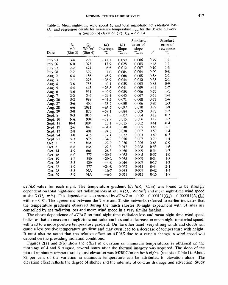
Table I lists the mean night-time wind speed at site 3 (Un, m/s) and total night-time net outgoing long-wave radiation at site 4 (Qn , Wh/m2) for the 30 nights when minimum air temperatures were observed at all 31 sites. Linear regressions of minimum air temperature on elevation in m above m.s.1. were performed for all nights. Slope ( b ) and intercept ( a ) values as well as correlation coefficients and error terms are given for each regression in Table I.

It can be seen that the slope (i.e. the temperature change with elevation, d T / d Z ) ranges from 0*097"C/m to -0-015"C/m and the intercept from -63.7 to 13.1. The standard error of regression ranges from 0-4 to 2.1"C with r2 values from 0.0 to 0.85.

High r2 values associated with large, positive d T / d Z values represent strong stratification and a significant terrain effect. The terrain effect is weak when r2 is close to zero. Small positive and negative d T / d Z values occur when strong ventilation causes the temperature gradient to approach dry adiabatic lapse rate conditions and local terrain effects have become insignificant. The role of elevation as a dominant topographic control on minimum air temperature is clearly evident from Table I .

On 24 nights dTldZ values obtained with the 31 site network may be compared with those obtained with the 7-station Ross recorder network. Excellent agreement was observed between d T / d Z values from the two networks. Mean d T / d Z values based on the 24 nights for the 7-site Ross recorder and 31-site alcohol-in-glass minimum thermometer networks were 0-0392 and 0.0415"C/m with standard deviations of 0.0285 and 0*0258"C/m, respectively.

During the 1982 winter season the 7-site Ross recorder network yielded minimum temperatures on about 100 nights covering a wide range of weather conditions. Linear regression was used to obtain a


Table I. Mean night-time wind speed Un and total night-time net radiation loss Q,, and regression details for minimum temperature T,,, for the 31-site network

as function of elevation ( Z ) : Tmin = bZ + a

Standard Standard un Qn (a 1 ( b ) error of error of

regression m/s Whim' Intercept Slope slope Date (Site 3) (Site 4) "C "Cim "Cim rz "C

July 23 July 26 July 27 July 28 Aug. 2 Aug. 3 Aug. 4 Aug. 5 Aug. 6 Aug. 7 Aug. 26 Aug. 27 Aug. 28 Aug. 29 Sept. 8 Sept. 10 Sept. 11 Sept. 12 Sept. 13 Sept. 24 Sept. 25 Oct. 2 Oct. 3 Oct. 14 Oct. 18 Oct. 19 Oct. 26 Oct. 27 Oct. 28 Oct. 29

3.4 6.0 2.2 2.2 6.4 7.7 3.6 4.4 3.6 2.2 5.2 3.6 6.6 3.0 9-3 NA

10.4 2.6 2.8 3.0 5.3 5.3 8.8 4.9 6.0 4.2 3.5 4.9 5.3 3.9

295 1073 474 329

1156 1275 755 443 95 1 546 999 460

1081 873

1056 904

1004 840 481 476 976 NA NA 661 777 350 429 777 NA NA

-41.7 - 17.9 -6.5

1.0 -46.9 -26.9 -40.1 -26.8 -40.9 -29.4 -44.5 -53.2 -63.7 -57.1 -1.0 - 12.7

13.1 -31.4 -24.8 - 14.4 - 34.2 -22-9 -27.3 -26.3 -20.1 -20.2 -4.8

-24.8 - 16.7 -6.5

0.059 0.028 0.012 0.004 0.066 0.044 0.058 0.041 0.058 0.045 0-071 0.080 0.097 0.084 0.007 0.015 .0*015 0-040 0.038 0.022 0.056 0.036 0.047 0.050 0.033 0-035 0.016 0.052 0.033 0.021

0.006 0.005 0.007 0.004 0.008 0.010 0.005 0.009 0.006 0-007 0.008 0.006 0.010 0.009 0.004 0.006 0.002 0.005 0-007 0.003 0-007 0-005 0-008 0.009 0.005 0-009 0.007 0.011 0.007 0.012

0.79 0.48 0.10 0.00 0.38 0.38 0.84 0.44 0.79 0-59 0.73 0.85 0.77 0.78 0.12 0.17 0.61 0.65 0.50 0.60 0-70 0.68 0.53 0.54 0.57 0.34 0.17 0.44 0.42 0.15

1.1 1.1 1.3 0.8 2.1 2.1 0-9 1.7 1.1 1-4 1.6 1.3 1.9 1-7 0.7 1.2 0.4 1.1 1.4 0.7 1-4 0.9 1.6 1.7 1.0 1.8 1.3 2.1 1.4 1.7

dTldZ value for each night. The temperature gradient (dTldZ, "Clm) was found to be strongly dependent on total night-time net radiation loss at site 4 ( e n , Wh/m2) and mean night-time wind speed at site 3 (Un, mls). This dependence is expressed by dTldZ = -0.02 + 0.0O0131(Qn) - O-OOOOll(U,Q,) with r = 0-84. The agreement between the 7-site and 31-site networks referred to earlier indicates that the temperature gradients observed during the much shorter 30-night experiment with 31 sites are controlled by net radiation loss and mean wind speed in a very similar fashion.

The above dependence of dTldZ on total night-time radiation loss and mean night-time wind speed indicates that an increase in night-time net radiation loss and a decrease in mean night-time wind speed, will lead to a more positive temperature gradient. On the other hand, very strong winds and clouds will cause a less positive temperature gradient and may even lead to a decrease of temperature with height. It must also be noted that the relative effect on d T / d Z due to a certain change in wind speed will depend on the prevailing radiation conditions.

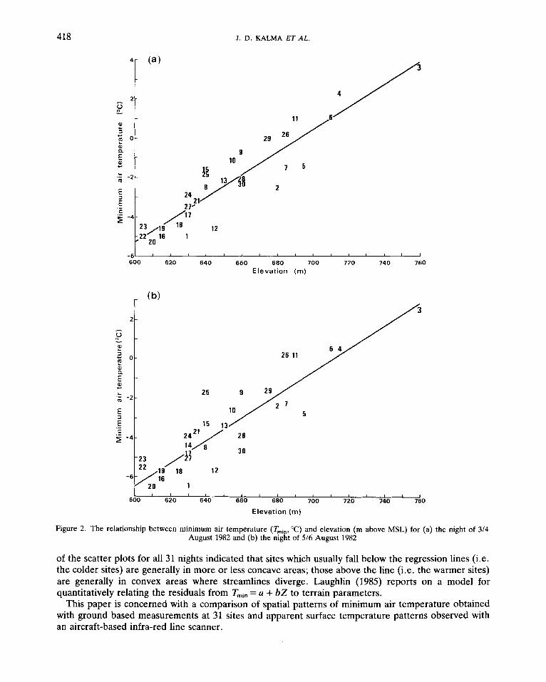
Figures 2(a) and 2(b) show the effect of elevation on minimum temperatures as obtained on the mornings of 4 and 6 August, several hours after the thermal imagery was acquired. The slope of the plot of minimum temperature against elevation was 0-058"Clm on both nights (see also Table I). About 82 per cent of the variation in minimum temperature can be attributed to elevation alone. The elevation effect reflects the degree of shelter and the intensity of cold air drainage and advection. Study

418 J. D. KALMA ET A t .

-6' ' 1

600 620 640 660 680 700 720 740 760 , , , I 1 ,

Elevation (m)

5

12

1 I , , , , , I , ( , I ,

600 620 640 660 680 700 720 740 760

Elevation (m)

Figure 2. The relationship between minimum air temperature (Tmin, "C) and elevation (m above MSL) for (a) the night of 3/4 August 1982 and (b) the night of 5 /6 August 1982

of the scatter plots for all 31 nights indicated that sites which usually fall below the regression lines (i.e. the colder sites) are generally in more or less concave areas; those above the line (i.e. the warmer sites) are generally in convex areas where streamlines diverge. Laughlin (1985) reports on a model for quantitatively relating the residuals from Tmin = a + bZ to terrain parameters.

This paper is concerned with a comparison of spatial patterns of minimum air temperature obtained with ground based measurements at 31 sites and apparent surface temperature patterns observed with an aircraft-based infra-red line scanner.


Table I indicates that the two nights on which thermal imagery data were acquired were quite similar; mean night-time wind speed was 3.6m/s on both nights and the night-time total net radiation losses during the nights of 314 and 516 August were 755 and 951 Wh/m2, respectively.

The simple regression model relating minimum temperatures to elevation was not considered accurate enough to obtain detailed minimum air temperature maps for the region. Instead, a surface fitting procedure was adopted which uses not only elevation but also map co-ordinates as independent input parameters.

Hutchinson et al. (1984a, b) have recently described the use of Laplacian smoothing spline functions of two or three independent variables for irregularly spaced solar radiation and wind-speed data. In the present study surfaces have been fitted by this method to the minimum temperature values obtained on 4 and 6 August. The fitted surfaces have an optimal trade-off between infidelity to the data as measured by the mean square residual from the data points and the roughness of the fitted surface as measured by the total curvature. The degree of smoothing imposed by the fitted surface is determined by minimizing the generalized cross-validation (GCV). In this application the two map co-ordinates and elevation were the independent variables. The fitted surfaces are based on map co-ordinates at 250m intervals and elevations to the nearest 10 m, obtained from a 1 : 25,000 topographic map. The standard errors

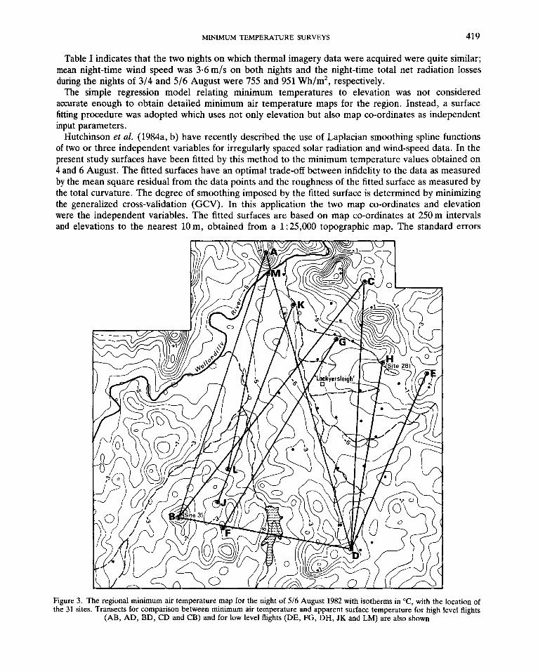
Figure 3. The regional minimum air temperature map for the night of 516 August 1982 with isotherms in "C, with the location of the 31 sites. Transects for comparison between minimum air temperature and apparent surface temperature for high level flights

(AB, AD, BD, CD and CB) and for low level flights (DE, FG, DH, JK and LM) are also shown


associated with any fitted surface value have been estimated as 0.66"C and 0.74"C for 4 and 6 August, respectively. The percentages of total variance accounted for are 96 and 95 for those surfaces. Note that these values show a significant improvement when compared with the r2 values of 0.84 and 0.79 obtained with the simple linear regression model (Table I). Computer techniques have been used to calculate and map contour lines from the above smoothing functions. The minimum air temperature maps for the nights of 314 August and 516 August produced in this way have been used for comparison with the thermal imagery obtained during those nights as discussed below. Part of the 516 August map is shown in Figure 3.

THERMAL IMAGERY

Measurements and calibration

Thermal imagery of the study area was obtained with an infra-red line scanner aboard an F-27 aircraft. The line scanner is a modified commercial Daedalus scanner with a roll-stabilization unit. The Hg-Cd-Te photoconductive detector in the scanner is sensitive to the 8-14 pm waveband. It is cooled to 77 K by liquid nitrogen to reduce the electrical noise. The spatial resolution of the instrument is 14 milliradians, i.e. 1.5 m at an elevation of 1000 m. Total field of view is 90". The image is recorded on magnetic tape for later analysis and enhancement.

High level imagery was obtained just before midnight on 3 August and low level imagery around midnight on the night of 5/6 August 1982. Logistical constraints prevented flights closer to the expected time of the minimum in air temperature.

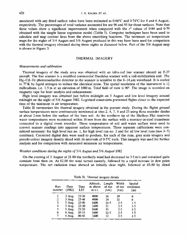
Table I1 summarizes the thermal imagery obtained in the present study. During the flights ground surface temperatures were continuously monitored at sites 2, 4, 7, 9 and 23 using Ross recorder diodes at about 2mm below the surface of the bare soil. At the northern tip of the Shelleys Flat reservoir water temperatures were monitored within 10 mm from the surface with a mercury-in-steel transducer connected to a digital event recorder. These temperatures of soil and water surface were used to convert scanner readings into apparent surface temperatures. Three separate calibrations were considered necessary: for high level run no. 1, for high level run no. 2 and for all low level runs (nos 3-7) combined. Corrected digital data were used to produce, for each of the runs, grey scale imagery and pseudo-colour imagery density sliced with 16 intervals of 0-5"C each. This imagery was used for further analysis and for comparison with measured minimum air temperatures.

Weather conditions during the nights of 314 August and 516 August 1982

On the evening of 3 August at 21.00 the northerly wind had decreased to 3.5 mls and remained quite constant from then on. At 02.00 the wind turned easterly, followed by a rapid increase in dew point temperature. The net radiation trace showed an initially clear night, followed at 03.00 by cloud

Table 11. Thermal imagery details

Run Date number (1982)

Time LST

1 3 Aug. 2 3 Aug. 3 5 Aug. 4 5 Aug. 5 5 Aug. 6 6 Aug. 7 6 Aug.

23.36 23.48 23.00 23.30 23.50 00.15 00.45

Altitude, m above

m.s.1.

4000 4000 1600 1600 1600 1600 1600

Length of run (km)

16 14 11.5 21 11 11.5 12

~~ ~

Spatial resolution

(m)

10 11 2.5 2.5 2.5 2-5 2.5

6 6 1.5 1.5 1.5 1.5 1-5


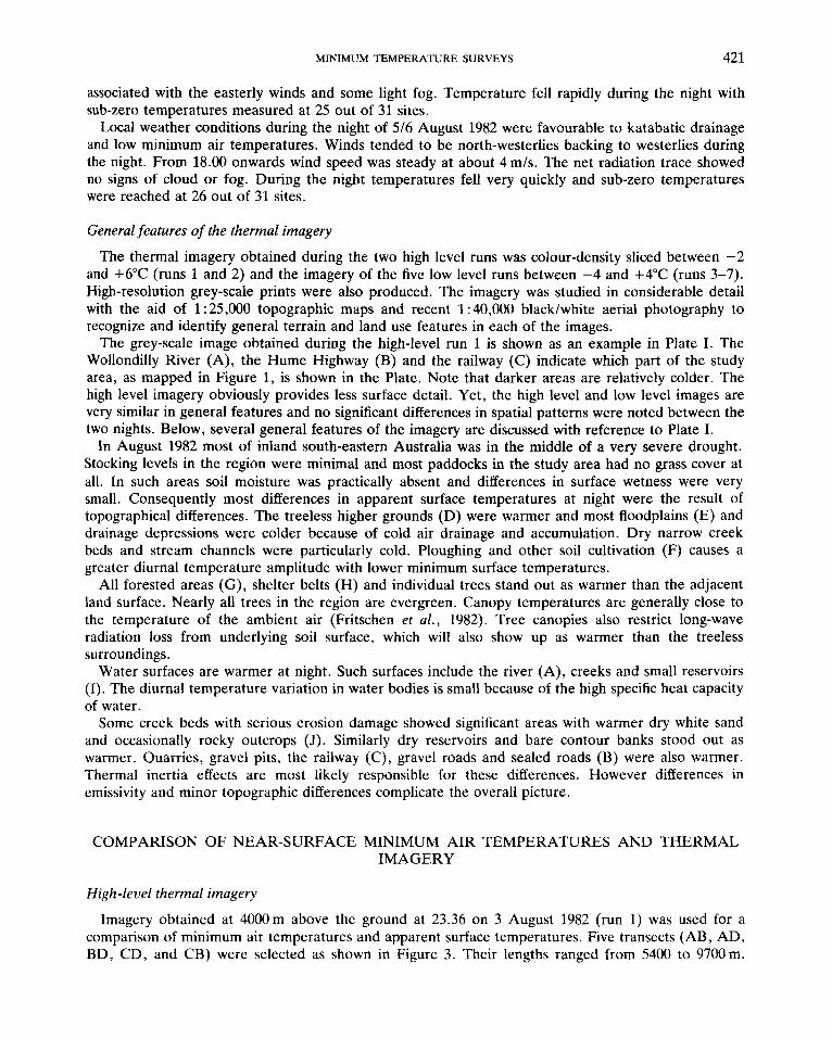
associated with the easterly winds and some light fog. Temperature fell rapidly during the night with sub-zero temperatures measured at 25 out of 31 sites.

Local weather conditions during the night of 5/6 August 1982 were favourable to katabatic drainage and low minimum air temperatures. Winds tended to be north-westerlies backing to westerlies during the night. From 18.00 onwards wind speed was steady at about 4m/s. The net radiation trace showed no signs of cloud or fog. During the night temperatures fell very quickly and sub-zero temperatures were reached at 26 out of 31 sites.

General features of the thermal imagery

The thermal imagery obtained during the two high level runs was colour-density sliced between -2 and +6"C (runs 1 and 2) and the imagery of the five low level runs between -4 and +4"C (runs 3-7). High-resolution grey-scale prints were also produced. The imagery was studied in considerable detail with the aid of 1 : 25,000 topographic maps and recent 1 : 40,000 black/white aerial photography to recognize and identify general terrain and land use features in each of the images.

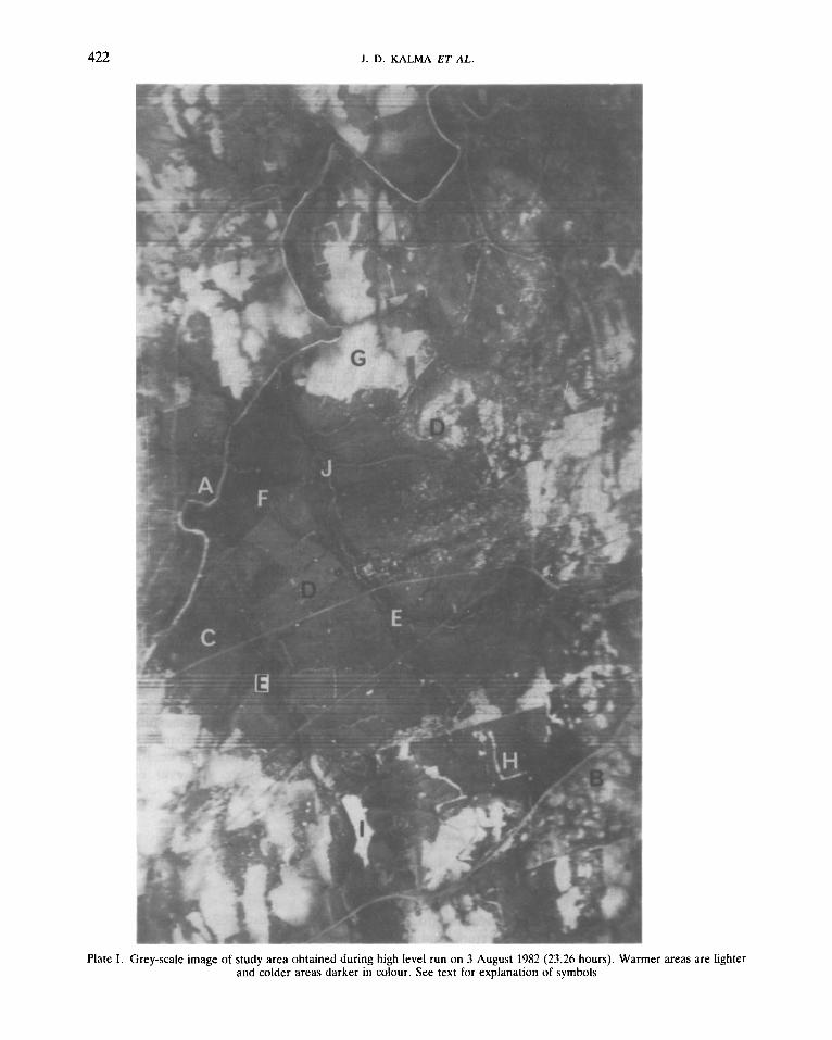
The grey-scale image obtained during the high-level run 1 is shown as an example in Plate I. The Wollondilly River (A), the Hume Highway (B) and the railway (C) indicate which part of the study area, as mapped in Figure 1, is shown in the Plate. Note that darker areas are relatively colder. The high level imagery obviously provides less surface detail. Yet, the high level and low level images are very similar in general features and no significant differences in spatial patterns were noted between the two nights. Below, several general features of the imagery are discussed with reference to Plate I.

In August 1982 most of inland south-eastern Australia was in the middle of a very severe drought. Stocking levels in the region were minimal and most paddocks in the study area had no grass cover at all. In such areas soil moisture was practically absent and differences in surface wetness were very small. Consequently most differences in apparent surface temperatures at night were the result of topographical differences. The treeless higher grounds (D) were warmer and most floodplains (E) and drainage depressions were colder because of cold air drainage and accumulation. Dry narrow creek beds and stream channels were particularly cold. Ploughing and other soil cultivation (F) causes a greater diurnal temperature amplitude with lower minimum surface temperatures.

All forested areas (G), shelter belts (H) and individual trees stand out as warmer than the adjacent land surface. Nearly all trees in the region are evergreen. Canopy temperatures are generally close to the temperature of the ambient air (Fritschen et al., 1982). Tree canopies also restrict long-wave radiation loss from underlying soil surface, which will also show up as warmer than the treeless surroundings.

Water surfaces are warmer at night. Such surfaces include the river (A), creeks and small reservoirs (I). The diurnal temperature variation in water bodies is small because of the high specific heat capacity of water.

Some creek beds with serious erosion damage showed significant areas with warmer dry white sand and occasionally rocky outcrops (J). Similarly dry reservoirs and bare contour banks stood out as warmer. Quarries, gravel pits, the railway (C), gravel roads and sealed roads (B) were also warmer. Thermal inertia effects are most likely responsible for these differences. However differences in emissivity and minor topographic differences complicate the overall picture.

COMPARISON OF NEAR-SURFACE MINIMUM AIR TEMPERATURES AND THERMAL IMAGERY

High -level thermal imagery

Imagery obtained at 4000m above the ground at 23.36 on 3 August 1982 (run 1) was used for a comparison of minimum air temperatures and apparent surface temperatures. Five transects (AB, AD, BD, CD, and CB) were selected as shown in Figure 3. Their lengths ranged from 5400 to 9700m.


Plate I. Grey-scale image of study area obtained during high level run on 3 August 1982 (23.26 hours). Warmer areas are lighter and colder areas darker in colour. See text for explanation of symbols


I 760- E -

720- -

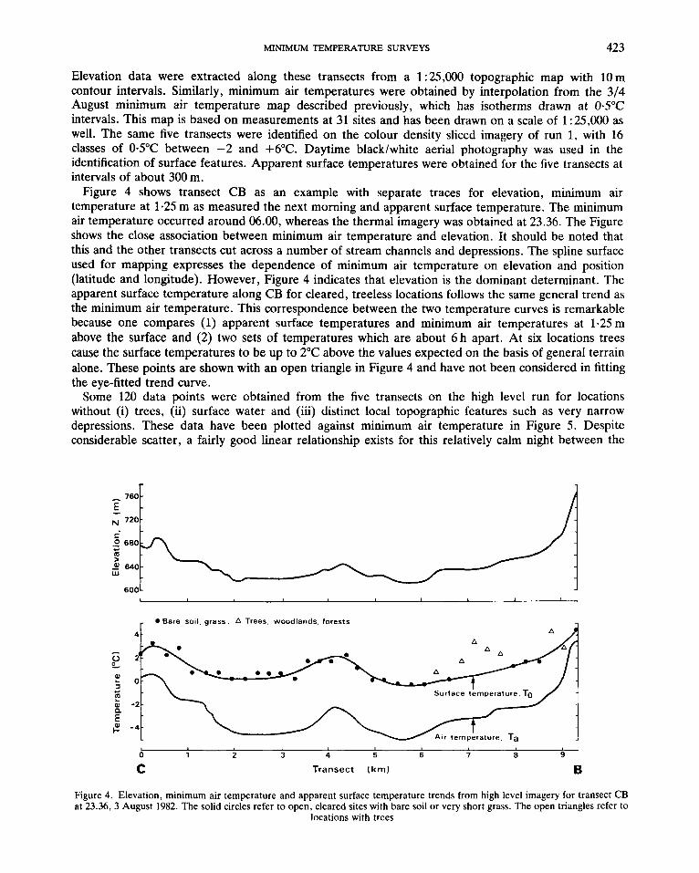
Elevation data were extracted along these transects from a 1:25,0o0 topographic map with 10m contour intervals. Similarly, minimum air temperatures were obtained by interpolation from the 3/4 August minimum air temperature map described previously, which has isotherms drawn at @5"C intervals. This map is based on measurements at 31 sites and has been drawn on a scale of 1 : 25,000 as well. The same five transects were identified on the colour density sliced imagery of run 1, with 16 classes of 0-5"C between -2 and +6"C. Daytime black/white aerial photography was used in the identification of surface features. Apparent surface temperatures were obtained for the five transects at intervals of about 300 m.

Figure 4 shows transect CB as an example with separate traces for elevation, minimum air temperature at 1.25 m as measured the next morning and apparent surface temperature. The minimum air temperature occurred around 06.00, whereas the thermal imagery was obtained at 23.36. The Figure shows the close association between minimum air temperature and elevation. It should be noted that this and the other transects cut across a number of stream channels and depressions. The spline surface used for mapping expresses the dependence of minimum air temperature on elevation and position (latitude and longitude). However, Figure 4 indicates that elevation is the dominant determinant. The apparent surface temperature along CB for cleared, treeless locations follows the same general trend as the minimum air temperature. This correspondence between the two temperature curves is remarkable because one compares (1) apparent surface temperatures and minimum air temperatures at 1.25 m above the surface and (2) two sets of temperatures which are about 6 h apart. At six locations trees cause the surface temperatures to be up to 2°C above the values expected on the basis of general terrain alone. These points are shown with an open triangle in Figure 4 and have not been considered in fitting the eye-fitted trend curve.

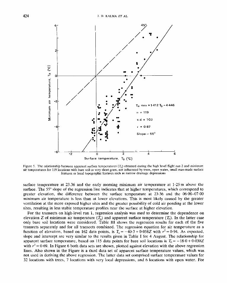
Some 120 data points were obtained from the five transects on the high level run for locations without (i) trees, (ii) surface water and (iii) distinct local topographic features such as very narrow depressions. These data have been plotted against minimum air temperature in Figure 5. Despite considerable scatter, a fairly good linear relationship exists for this relatively calm night between the

r

- 0 Bare soil, grass, A Trees, woodlands. forests

4 -

- 0 Bare soil, grass, A Trees, woodlands. forests

4 -

L I 0 1 2 3 4 5 6 7 8 9

C Transect (km) B

Figure 4. Elevation, minimum air temperature and apparent surface temperature trends from high level imagery for transect CB at 23.36, 3 August 1982. The solid circles refer to open, cleared sites with bare soil or very short grass. The open triangles refer to

locations with trees


/’ /

/ /

” -2 0 2 4 6 Surface temperature. TO (“c)

Figure 5. The relationship between apparent surface temperatures (TJ obtained during the high level flight run 2 and minimum air temperatures for 119 locations with bare soil or very short grass, not influenced by trees, open water, small man-made surface

features or local topographic features such as narrow drainage depressions

surface temperature at 23.36 and the early morning minimum air temperature at 1.25m above the surface. The 55” slope of the regression line indicates that at higher temperatures, which correspond to greater elevation, the difference between the surface temperature at 23.36 and the 06.00-07.00 minimum air temperature is less than at lower elevations. This is most likely caused by the greater ventilation at the more exposed higher sites and the greater possibility of cold air ponding at the lower sites, resulting in less stable temperature profiles near the surface at higher elevation.

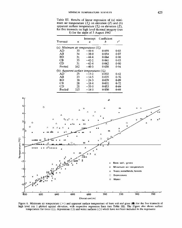
For the transects on high-level run 1, regression analysis was used to determine the dependence on elevation Z of minimum air temperature (T’) and apparent surface temperature (To). In the latter case only bare soil locations were considered. Table 111 shows the regression results for each of the five transects separately and for all transects combined. The regression equation for air temperature as a function of elevation, based on 162 data points, is Ta = -40.3 + 0.0582 with r 2 = 0.94. As expected, slope and intercept are very similar to the results given in Table I for 4 August. The relationship for apparent surface temperature, based on 115 data points for bare soil locations is 7;) = -18.0 + 0.0302 with r2 = 0.69. In Figure 6 both data sets are shown, plotted against elevation with the above regression lines. Also shown in the Figure is a third data set of apparent surface temperature values, which was not used in deriving the above regression. The latter data set comprised surface temperature values for 32 locations with trees, 7 locations with very local depressions, and 6 locations with open water. For


CL 0

Table 111. Results of linear regression of (a) minimum air temperature (T,) on elevation (2) and (b) apparent surface temperature (T,) on elevation ( Z ) , for five transects on high level thermal imagery (run

1) for the night of 3 August 1982

Intercept Coefficient Transect n a b

(a) Minimum air temperatures (T,) AD 33 -40.4 0.059 AB 34 -38,O 0.054 BD 31 -44.4 0.064 CB 35 -42,2 0.061 CD 31 -42.4 0.062 Pooled 162 -40.3 0.058

AD 25 -13-2 0.022 AB 23 -14.5 0.025 BD 18 -24.3 0.039 CB 28 -18.4 0.031 CD 21 -33.0 0.053 Pooled 115 -18.0 0.030

(b) Apparent surface temperatures (T,,)

r2

0.93 0.97 0.98 0.93 0.90 0.94

0-42 0-76 0.89 0.72 0.69 0.69

1 1 I I I I I 1 1 1 I

620 640 660 680 700 720 740 760

Elevation (m)

Figure 6. Minimum air temperature ( x ) and apparent surface temperature of bare soil and grass (0) for the five transects of high level run 1 plotted against elevation, with respective regression lines (see Table 111). The Figure also shows surface

temperature for trees (A) , depressions (0) and water surfaces (0) which have not been included in the regression


each data point in this third data set the derivation from the line = -18.0 + 0.0302 was determined. It was found that trees caused on average an increase in surface temperature of 1.5"C, with individual values ranging between an increase of 24°C and a decrease of 1.4"C. Local depressions (not detectable on 1:25,000 map with 10m contours) caused on average a decrease of 1.5"C with a range between decreases of 2-7"C and 0.4"C. Water surfaces show increases between 0.1 and 4.2"C with an average increase of 2.3"C.

Low-level thermal imagery

Low level imagery was obtained at a height of 1600m on runs 3-7 during the night of 516 August 1982. The overall agreement between the spatial distribution of apparent surface temperature as obtained during runs 3-7 and minimum air temperatures mapped for the night of 516 August is very good. For a detailed comparison between the surface temperatures and air temperatures, the transects DE, FG, DH, JK and LM (see Figure 3) were selected for runs 3-7, respectively. Their lengths range from 6025 to 6925 m. Elevation data were obtained for these transects from the 1 : 25,000 topographic map with 10 m contour intervals. Minimum air temperatures along the transects were obtained for the night from the minimum air temperature map for 5/6 August 1982, referred to above. The transects were identified on the colour imagery of runs 3-7, and surface temperatures were read off at intervals of about 85 m. Note that 16 classes were used of 0-5"C between -4 and +4"C.

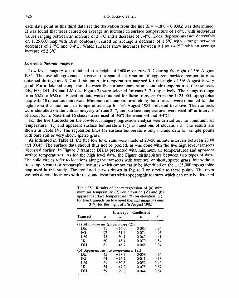
For the five transects on the low-level imagery regression analysis was carried out for minimum air temperature (T,) and apparent surface temperature (T,) as functions of elevation Z. The results are shown in Table IV. The regression lines for surface temperature only include data for sample points with bare soil or very short, sparse grass.

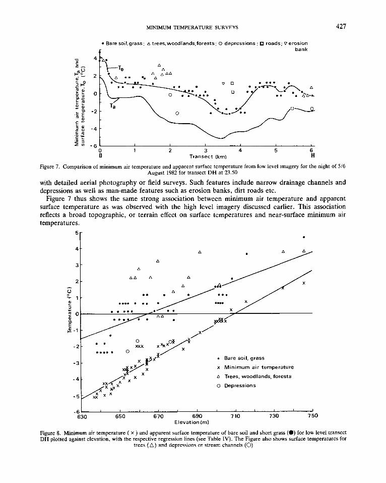
As indicated in Table 11, the five low level runs were made at 20-30 minute intervals between 23.00 and 00.45. The surface data should thus not be pooled, as was done with the five high level transects discussed earlier. In Figure 7 transect DH is presented with minimum air temperatures and apparent surface temperatures. As for the high level data, the Figure distinguishes between two types of data. The solid circles refer to locations along the transects with bare soil or short, sparse grass, but without trees, open water or topographic features which cannot easily be identified on the 1 : 25,000 topographic map used in this study. The eye-fitted curves drawn in Figure 7 only refer to these points. The open symbols denote locations with trees; and locations with topographic features which can only be detected

Table IV. Results of linear regression of (a) minimum air temperature (T.) on elevation (Z) and (b) apparent surface temperature (To) on elevation (Z), for five transects on low level thermal imagery (runs

3-7) for the night of 516 August 1982 ~~~

Intercept Coefficient Transect n 11 b r2

~~

(a) Minimum air temperatures (T,) DE 71 -56.0 0.080 FG 97 -51.4 0,074 LM 75 -30.1 0.040 JK 80 -48.4 0-070 DH 81 -46.2 0.065

(b) Apparent surface temperatures (T,) DE 45 -38.7 0.058 FG 64 -26.2 0-041 LM 61 -30.5 0.050 JK 54 -47.2 0-075 DH 59 -29.3 0-044

0.94 0.95 0.41 0.84 0.94

0.64 0.18 0.40 0.57 0-64


Bare soil,grass; A trees,woodlands,forests; 0 depressions ; roads; v erosion bank

A A

A A A A

v n 0 0 . . 0 .n A

2

-6 I I I I

0 1 2 3 4 5 6 D Transect (Itm) H

Figure 7. Comparison of minimum air temperature and apparent surface temperature from low level imagery for the night of 5 / 6 August 1982 for transect DH at 23.50

with detailed aerial photography or field surveys. Such features include narrow drainage channels and depressions as well as man-made features such as erosion banks, dirt roads etc.

Figure 7 thus shows the same strong association between minimum air temperature and apparent surface temperature as was observed with the high level imagery discussed earlier. This association reflects a broad topographic, or terrain effect on surface temperatures and near-surface minimum air temperatures.

0

4 1

- 4

-5 ::I_ X

Bare soil, grass Minimum air temperature

Trees, woodlands, forests

Depressions

-6 I I I I I 1 L I , I I I 630 650 670 690 7 10 7 30 7 50

Elevation (m)

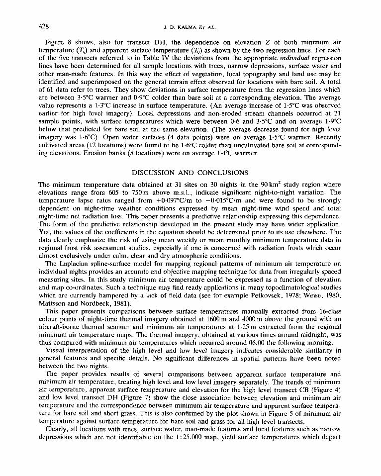
Figure 8. Minimum air temperature ( X ) and apparent surface temperature of bare soil and short grass (0) for low level transect DH plotted against elevation, with the respective regression lines (see Table IV). The Figure also shows surface temperatures for

trees (A) and depressions or stream channels (0)


Figure 8 shows, also for transect DH, the dependence on elevation Z of both minimum air temperature (T,) and apparent surface temperature (To) as shown by the two regression lines. For each of the five transects referred to in Table IV the deviations from the appropriate individual regression lines have been determined for all sample locations with trees, narrow depressions, surface water and other man-made features. In this way the effect of vegetation, local topography and land use may be identified and superimposed on the general terrain effect observed for locations with bare soil. A total of 61 data refer to trees. They show deviations in surface temperature from the regression lines which are between 3.5"C warmer and 0-9"C colder than bare soil at a corresponding elevation. The average value represents a 1.3"C increase in surface temperature. (An average increase of 105°C was observed earlier for high level imagery). Local depressions and non-eroded stream channels occurred at 21 sample points, with surface temperatures which were between 0.6 and 3.5"C and on average 1.YC below that predicted for bare soil at the same elevation. (The average decrease found for high level imagery was 1-6°C). Open water surfaces (4 data points) were on average 1-5"C warmer. Recently cultivated areas (12 locations) were found to be 1.6"C colder than uncultivated bare soil at corresponding elevations. Erosion banks (8 locations) were on average 1.4"C warmer.

DISCUSSION AND CONCLUSIONS

The minimum temperature data obtained at 31 sites on 30 nights in the 90 km2 study region where elevations range from 605 to 750 m above m.s.l., indicate significant night-to-night variation. The temperature lapse rates ranged from +0.097"C/m to -0.015"Clm and were found to be strongly dependent on night-time weather conditions expressed by mean night-time wind speed and total night-time net radiation loss. This paper presents a predictive relationship expressing this dependence. The form of the predictive relationship developed in the present study may have wider application. Yet, the values of the coefficients in the equation should be determined prior to its use elsewhere. The data clearly emphasize the risk of using mean weekly or mean monthly minimum temperature data in regional frost risk assessment studies, especially if one is concerned with radiation frosts which occur almost exclusively under calm, clear and dry atmospheric conditions.

The Laplacian spline-surface model for mapping regional patterns of minimum air temperature on individual nights provides an accurate and objective mapping technique for data from irregularly spaced measuring sites. In this study minimum air temperature could be expressed as a function of elevation and map co-ordinates. Such a technique may find ready applications in many topoclimatological studies which are currently hampered by a lack of field data (see for example Petkovsek, 1978; Weise, 1980; Mattsson and Nordbeck, 1981).

This paper presents comparisons between surface temperatures manually extracted from 16-class colour prints of night-time thermal imagery obtained at 1600 m and 4000 m above the ground with an aircraft-borne thermal scanner and minimum air temperatures at 1.25 m extracted from the regional minimum air temperature maps. The thermal imagery, obtained at various times around midnight, was thus compared with minimum air temperatures which occurred around 06.00 the following morning.

Visual interpretation of the high level and low level imagery indicates considerable similarity in general features and specific details. No significant differences in spatial patterns have been noted between the two nights.

The paper provides results of several comparisons between apparent surface temperature and minimum air temperature, treating high level and low level imagery separately. The trends of minimum air temperature, apparent surface temperature and elevation for the high level transect CB (Figure 4) and low level transect DH (Figure 7) show the close association between elevation and minimum air temperature and the correspondence between minimum air temperature and apparent surface temperature for bare soil and short grass. This is also confirmed by the plot shown in Figure 5 of minimum air temperature against surface temperature for bare soil and grass for all high level transects.

Clearly, all locations with trees, surface water, man-made features and local features such as narrow depressions which are not identifiable on the 1 : 25,000 map, yield surface temperatures which depart


from the trends and relationships established for bare soil and short grass. The linear regression results of Tables 111 and IV express the elevation dependence of minimum air temperature and apparent surface temperature of bare soil and short grass for all high level and low level transects. This procedure makes it possible to calculate the departures from the regression lines for all locations other than those with bare soil or short grass. Average values show that trees cause increases of 1.5”C and 1~3°C for high level and low level, respectively. Local depressions cause average decreases of 1-5” and 1.9”C. The corresponding values for water surfaces are average increases of 2-3” and 1~5°C in the apparent surface temperature.

Two specific areas of concern fall outside the scope of the present paper. First, problems associated with the conversion of digital radiance data have been circumvented by direct comparison of the digital radiance data with measured surface temperatures at the time of the flights at a number of locations in the study area. Secondly, the effect of spatial differences in surface emissivity ( E ) has not been addressed in this paper: it has been tacitly assumed that emissivity differences across the study area are generally small, with the emissivity of most vegetative covers exceeding 0.97.

The results of the present study indicate that remote sensing may become an important aid in understanding spatial distribution patterns in surface temperature and near-surface air temperature and hence could be of great value in local scale frost risk assessment. This paper has not been concerned with the use of thermal imagery in predicting minimum air temperatures per se. For predictive purposes remotely sensed surface temperatures should be used with atmospheric boundary layer models which simulate latent, sensible and radiative heat transfer at the surface for the most appropriate range of surface conditions.

ACKNOWLEDGEMENTS

We gratefully acknowledge the technical field assistance of H. Alksnis, P. J . Daniel and D. P. Richardson. The co-operation of M. F. Hutchinson and M. E. Johnson in the surface fitting and contour mapping of the minimum air temperatures is greatly appreciated. We also thank the landholders in the study region for their co-operation.

REFERENCES

Bagdonas, A., George, J. C. and Gerber, J. F. 1978. ‘Techniques for frost prediction and frost protection’, W.M.O. Tech. Note

Byrne, G. F . , Kalma, J . D. and Streten, N. A. 1984. ‘On the relation between HCMM satellite data and temperatures from

Caselles, V., Gandia, V. and Melia, J . 1983. ‘Significance of apparent temperature measurements carried out by the HCMM

Chen, E., Allen Jr, L. H . , Bartholic, J. F., Bill Jr, R. G. and Sutherland, R. A. 1979. ‘Satellite-sensed winter nocturnal

Chen, E., Allen Jr, L. H., Bartholic, J. F. and Gerber, J. F. 1982. ‘Delineation of cold-prone areas using night-time SMS/GOES

Chen, E., Allen Jr, L. H., Bartholic, J. F. and Gerber, J . F. 1983. ‘Comparison of winter-nocturnal geostationary satellite

Endlicher, W. 1980. ‘Gelandeklimatologische Untersuchungen im Weinbaugebiet des Kaiserstuhls’, Berichte des Deutschen

Fritschen, L. J., Balick, L. K. and Smith, J. A. 1982. ‘Interpretation of infrared night-time imagery of a forested canopy’, J .

Hutchinson, M. F., Booth, T. H., McMahon, J. P. and Nix, H. A. 1984a. ‘Estimating monthly mean values of daily total solar

Hutchinson, M. F., Kalma, J. D. and Johnson, M. E. 1984b. ‘Monthly estimates of windspeed and windrun for Australia’, J .

Kalma, J. D., Byrne, G. F. , Johnson, M. E. and Laughlin. G. P. 1983. ‘Frost mapping in southern Victoria: an assessment of

Laughlin, G. P. 1985. ‘Local scale frost assessment from simple land and climate data’, Ph.D. thesis, submitted to University of

Mahrt, L. and Heald, R. C. 1983. ‘Nocturnal surface temperature distribution as remotely sensed from low flying aircraft’, Agric.

No. 157, W.M.O., Geneva.

standard meteorological sites in complex terrain’, Inf. J . Remote Sensing, 5 , 65.

satellite over areas of vegetation’, Agric. Meteorol., 30, 77.

temperature patterns of the Everglades Agricultural Area’, J . Appl. Meteorol., 18, 992.

thermal data: effect of soils and water’. J . Appl. Meteoroi., 21, 1528.

infrared-surface temperature with shelter height temperature in Florida’, Remote Sensing Enuiron., 13, 313.

Wetterdienstes Nr 150, Offenbach am Main.

Appl. Meteorol., 21, 730.

radiation for Australia’, Solar Energy, 32, 277.

Climatol., 4, 31 1.

HCMM thermal imagery’, J . Clirnatol., 3, 1.

New South Wales, Sydney.

Meteorol., 28, 99.

430 J. D. KALMA ET A L

Mattsson, J. 0. and Nordbeck, S. 1981. ‘Modelling cold air patterns’, Lund Studies in Geography Ser. A , Physical Geography,

Nixon, P. R. and Hales, T. A. 1975. ‘Observing cold-night temperatures of agricultural landscapes with an airplane-mounted

Petkovsek, Z. 1978. ‘Relief meteorologically relevant characteristics of basins’, Zeirschrift fur Meteorologie, 28, 233. Weise, A. 1980. ‘Moglichkeiten gelandeklimatischer Systematisierung’, Geographkche Berichte, 96, 179.

59, 119.

radiation thermometer’, J . Appl. Meteorol., 14, 498.

minimum temperature surveys based on near-surface air temperature measurements and airborne thermal...

Documents