minimum needs and effective consumption...

1

Report of The Task Force on Projections

of Minimum needs and

Effective consumption demand

Perspective Planning Division Government of India Planning Commission

New Delhi January 1979

2

ACKNOWLEDGEMENT

On behalf of the Task Force on Projections of Minimum Needs and Effective Consumption Demands constituted by the Planning Commission. I express my gratitude to Prof. Raj Krishna, Member, Planning Commission, who in his inaugural address had very succinctly outlined the scope and objectives of initiating the construction of a Model of Private Consumption in the 1978-83 Plan in its proper perspective.

I am thankful to all the members of the Task Force whose active deliberations helped in the construction of the framework of the consumption model for 1978—83 Plan. Dr. Y. K. Alagh, Adviser, Perspective Planning Division and Chairman of the Task Force, provided overall guidance and coordination. Prof. R. Radhakrishna and Shri G. V. S. N. Murthy of the Sardar Patel Institute of Economic and Social Research, Ahmedabad and Dr. D. Coondoo of the Indian Statistical Institute, Calcutta, extended valuable cooperation and collaboration in providing inputs in formulating the consumption Model. Prof. S. D. Tendulkar, jointly with Prof. Radhakrishna, prepared suggestions for further work. Prof. D. B. Gupta helped in the formulation of minimum

norms. Dr. Jayanta Roy, Consultant, Perspective Planning Division, edited the Report. I am grateful to all of them.

I am extremely grateful to my colleagues in the Perspective Planning Division of the Planning Commission who have helped and sincerely contributed to the preparation of this Report. Special mention must be made of Dr. B. M. Mahajan, Shri A. Chibber and Shri K. L. Datta. Dr. Mahajan assisted by S/Shri K. L. Datta and M. M. Gupta had completed the study on Poverty Line earlier started by Shri P. S. Sangwan. Dr. Mahajan in particular and Shri Rajaram Dasgupta had rendered considerable assistance in drafting this Report.

I am also thankful to the staff of the Computer Services Division of the Planning Commission for extending valuable assistance in programming work.

K. C. MAJUMDAR Convenor

3

CONTENTS

Chapter No. PAGE No. 1. Task Force—Terms of Reference and Composition 1 2. Methodological Framework 3 3. Demand Systems 5 4. Projection of Private Consumption by Input-Output Sectors 10 5. Recommendations and Future Direction of Work 14 6. Appendices 17

Technical Appendix 1—Engel Curves/Demand functions 49

Technical Appendix 2—Price Adjustment of Demand Function Parameters from 1973-74 prices to 1976-77 prices 51

Annexure I—Comments of Prof. N. S. lyengar and Comments on the Remarks of Prof, lyengar by Dr. R. Radhakrishna 52

Annexure II—Expected Value of Demand by the other two forms 54

4

CHAPTER 1

TASK FORCE—TERMS OF REFERENCE AND COMPOSITON

A number of useful research studies on consumer demand-behavioristic /effective, and normative — have been, and are being conducted both at the national an£ regional levels as well as for certain occupational groups etc., by research institutions, like the Indian Statistical Institute, Calcutta; Institute of Economic Growth, Delhi; Sardar Patel Institute of Economic and Social Research, Ahmedabad and by research workers in individual capacities.

1.1 Prof. N. S. lyengar developed a method of computing Engel ''elasticities from concentration curves [Econometrica (I960)]. This paper specifying the assumption of lognormality of the distribution of the monthly per capita consumer expenditure and considering the Lorenz curve, foe aggregate consumption and/ r the specific concentration curve for commodity consumption, derives Engel elasticities for various, items of consumer expenditure.

1.2 The Indian Statistical Institute, Calcutta, estimated Engel curves, for various expenditure categories based on National Sample Survey (NSS) data from the 7th to 22nd Rounds. The work relating to regional comparison of food-grains consumption for major items of consumption for 15 major states for both quantity and value based on NSS data relating to 13th, 17th and 18th Rounds was also undertaken by the Institute. In addition, theInstitute developed constant elasticities for 101 items of consumption based on value data for 18th Round at the all-India level; for 80 items of consumption in case of West Bengal; for 45 items of consumption for major states and for certain specified items of consumption for occupational groups like cultivators, agricultural labourers, other agricultural and non-agricultural occupations for rural areas.

1.3 The Sardar Patel Institute of Economics and Social Research developed the Linear Expenditure System in the frame work of a total demand model for lower, middle and higher income groups of population as well as for all groups combined separately for rural and urban areas, based on the consumer expenditure data available from the 2nd to 20th Round of the NSS.

1.4 A, poverty line in the context. of India was first given by a distinguished working group set up by the Planning Commission Government of India, in July 1962. Later on poverty lines under different assumptions were estimated by Professors V. M. Dandekar and N. Rath1*, A. Rudra2†, P. Bardhan3‡ and others.

1.5 In this. context, it was felt that if the results of these studies could be brought together at one place, it should; be possible to develop ideas to articulate a private consumption model — at 'national as well as regional levels for the next Five Year Plan. To this end, it was decided to set up a Task Force on Projections of Minimum Needs and Effective Consumption Demands to serve as a focal point.

1.6 The terms of reference of the Task Force are as follows —

"to examine theexisting structural studies on consumption patterns and standards of living and the: minimum needs with particular reference to the poorer, sections of the population for the nation! as a whole, arid its different regions separately by rural and urban areas; on the basis of the above studies, to forecast the national and regional structure and pattern of consumption levels and standards for the end of the Sixth Plan and subsequent perspective plan taking into consideration the basic minimum needs as wellas effective consumption demand".

1.7 The following is the composition of the Task Force: —

1. Dr. Y. K. Alagh — Chairman Adviser (PP) Planning Commission New Delhi.

2. Dr. D. Coondoo — Member. Economic Research Unit Indian Statistical Institute Calcutta— 700 035

* Dandekar V. M. and Rath N.- Poverty in India. † Rudra A. 'Minimum Level of Living—A Statistical Examination' in Poverty and Income Distribution in India (ed) T.N. Srinivasan and P. K. Bardhan ‡ Bardhan P. 'Incidence of Poverty in Rural India' in Poverty and Income Distribution in India (ed) T.N. Srinivasan & P.K. Bardhan

5

3. Dr. D. B. Gupta —Member.

Institute of Economic Growth University Enclave Delhi— 110 007.

4. Prof. N. S. lyengar — Member. Department of Economics Osmania University Hyderabad— 500 007.

5. Dr. L. R. Jain — Member. Indian Statistical Institute 7, S. J. S. Saasanwal Marg New Delhi— 110 029.

6. Shri G. V. S. N. Murty —Member. Sardar Patel Institute of Economic & Social Research Navrangpura, Ahmedabad—380009.

7. Prof. R. Radhakrishna —Member. Sardar Patel Institute of Economic & Social Research Navrangpura, Ahmedabad—380009.

8. Dr. S. D. Tandulkar —Member. Indian Statistical Institute 7, S. J. S. Sansanwal Marg New Delhi— 110 029.

9. K. C, Majumdar* — Member. Director (PP) Planning Commission New Delhi— 110 001.

Prof. P. V. Sukhatme of the Maharashtra Association for the Cultivation of Science who was abroad at the time of constitution of -the Task Force, was subsequently included as Member of the Task Force on his return to India.

1.8 Chapter 2 sets out the recommendations of the Task Force. Chapter 3 discusses demand systems to formulate Private Consumption Model used in the Input-Output Model considered for the Five Years Plan, 1978— 83. Chapter 4 estimates commodity consumer demand targets for the normative and preferred versions of the 89 sector Input-Output Model separately for the terminal years of the new, Plan (1978 — 83) and the perspective period (1983—88). Chapter 5 deals, "with suggestions for further work.

1.9 A number of supporting Appendices relating to technical notes, and| detailed tables supplement and complement the material contained in the text of the report.

6

CHAPTER 2 METHODOLOGICAL FRAME-WORK

The Task Force held its first meeting during 8th to 10th August, 1977 in the Planning Commission, New Delhi, under the chairmanship of Prof. Raj Krishna, Member, Planning Commission, and the last meeting on 23rd April, 1979.

2.1.1 Prof. Raj Krishna, in his inaugural address, outlined the scope and objective of the Private Consumption Model for the new Plan. He underlined the importance of distinction between normative and effective/behaviouristic demand on the one hand and between demand for traded private and non-traded public goods on the other. Regarding the former, he emphasised that the model should postulate the mini-mum desirable normative consumption for the people below the poverty line, both in rural and urban areas. The Model should reflect effective demand for the people above the poverty line. Appreciating the difficulties encountered in estimating the demand for non-traded public goods and services like drinking water, sanitation, health and education, he nevertheless underscored the importance of measuring the demand for such goods. He stated that minimum needs particularly of non-traded public goods and services cannot strictly be defined in monetary terms unless certain minimum standards for these are accepted.

2.1.2 He felt that change in price structure does influence the demand for commodities and, as such, while making demand projections, attempt should be made to consider this factor as well. Furthermore, for the Approach Paper, one of the variants for demand projections could be based on the assumption of no change in income distribution.

2.2 Based on the consensus of opinion emerging out of the deliberations of this Meeting, two main decisions were taken with regard to the methodology of estimation of commodity wise private consumption effective/behaviouristic and normative, for the Sixth Plan: —

i) Linear Expenditure System (LES), which is a total demand system and possesses, inter alia, the property of additivity should be used to estimate consumer demand for broad groups of commodities. Disaggregative demands for individual commodities constituting each broad group should be

worked out appropriately on the basis of best-fitting Engel curves, so as to add to a the group totals obtained on the basis of LES model, LES group totals thus serving as a control for estimating disaggregative demands with in the group. Alternatively, Fifth Five, Year Plan consumption model based on consumption proportions within each expenditure class — without, however, considering any re-distribution of ex-penditure could be used. It was decided that on the basis of the NSS time series of cross section data on consumer expenditure from various rounds upto 28th Round in 1973-74, LES parameters for as many broad groups of commodities as possible would be estimated by Shri G. V. S. N. Murty of the Sardar Patel Institute of Economic and Social Research, Dr. D. Coondoo of the Indian Statistical Institute, Calcutta, would furnish estimates of demand functions /Engel curve parameters on the basis of NSS consumer expenditure data for the 28th Round to workout disaggregative effective demand within various LES groups corresponding to the 89 input-output sectoral classification of the model to be used for the new plan. For this work, a Sub-group of the Task Force was formed, consisting of Dr. K.C. Majumdar, Shri Murty and Dr. Coondoo. It was aggreed that Shri Murty and Dr. Coondoo would work at Planning Commission in close collaboration and consultation with Dr. K. C. Majumdar, Chief (the then Director), Perspective Planning Division of the Planning Commission. The LES and Engel curve parameters would be estimated separately for the rural and urban areas and within each area separately for the population below the poverty line and above the poverty line.

ii) A paper giving estimates of minimum needs based on NSS data in physical terms for the 28th Round (1973-74) and other related studies would be prepared by Dr. D. B. Gupta of the Institute of Economic Growth, Delhi, in collaboration with the Perspective

7

Planning Division, Planning Commission. The calorie and the protein content of the per capita consumption of various food items by different expenditure classes would be estimated by the Perspective Planning Division on the suggestions made by Dr. D. B. Gupta. The per capita expenditure class, which satisfied the minimum calorie require-ments on nutritional consideration, would provide the cut-off point delineating the poverty line. The per capita consumption of various goods and services pertaining to this expenditure class would constitute normative demand. One variant of the consumption model would be based on the assumption that the population below the poverty line will have the normative consumption and that above it the be-haviouristic one, separately for the rural and urban areas.

2.3 Following additional points also emerged in the course of the discussions : —

i) A sub-group of the Task Force comprising Dr. Tendulkar of the Indian Statistical Institute, New Delhi and Professor R. Radha krishna of Sardar Patel Institute of Economic and Social Research was constituted to prepare a paper surveying the existing literature on consumption function and demand projections;

ii) Need for adopting norms in respect of non-traded public goods like housing, primary education, drinking water, clothing and medicines was felt;

iii) Views should also be expressed on the distribution policy that should be adopted regarding food, sugar,clothing, housing, education, health and miscellaneous civic services; and

iv) Regional focus should be brought out in the estimation of demand for various essential commodities in the final report.

2.4 Certain additional studies were also sug-gested:—

(i) The scope of the LES should be widened to encompass more commodity groups preferably comparable with input-output classification using the latest NSS data and, in turn, its parameters reestimated;

(ii) LES be reestimated for various groups of expenditure classes taking into consideration the change in expenditure classes over different rounds due to price changes;

(iii) Estimation of different demand functions /Engel curves should be attempted for as many commodities as possible, using available data of the various NSS rounds and

(iv) Regional specific norms of minimum needs should be estimated both for essential traded private goods and non-traded public goods.

8

CHAPTER 3 DEMAND SYSTEMS

Introduction

This Chapter within die frame work delineated in Chapter 2 presents, the methodology to estimate targets of consumption for the 89 sectors of the input-output model embodied in the terminal year, 1982-83 of the New Five Year Flan (1978 — 83) and in the terminal! year, 1987-88 of the perspective period (1983 — 88). For this purpose, two types of demand systems, Normative and Effective, have been considered.

Normative Demand System

3.2 Normative Demand ensures a minimum per capita consumption of different goods and services particularly of food items that will satisfy a desirable nutritional requirements in terms of calories per person per day. This normative demand has been considered specially for the people below poverty line.

4.2.1 The question of defining the poverty line was first mooted by the Indian Labour Conference in 1957. A distinguished Working Group was set-up by the Planning Commission, Government of India, in July, 1962, to deliberate on the question of what should be regarded as the nationally desirable minimum level of consumer expenditure. The Working Group appears to have taken into account the recommendation of balanced diet made by the Nutrition Advisory Committee of the Indian Council of Medical Research in 1958, and came to the view that in order to provide the minimum nutritional diet in terms of calorie intake, and to allow for a modest degree of items other than food, the national minimum consumption expenditure per household of 5 persons should not be less than Rs.100 per month at 1960-61 prices, i.e., Rs.20 per capita per month. The Group suggested that for urban areas, the minimum should be raised to Rs.25 per capita in view of the higher cost of living there. By implication, this meant that the corresponding amount in the rural areas would work out to Rs.18.9.

3.2.2 In a study conducted by Dandekar and Rath in 1971, an intake of 2,250 calories per capita per day was assured as adequate under the Indian conditions both in rural and urban areas. On the basis of National Sample Survey data on consumer expenditure, the study revealed that an average

annual per capita expenditure of Rs.170.8 or equivalently Rs.14.2 per capita per month at 1960-61 prices would suffice to meet these calorie requirements in the rural areas. The corresponding figures in the urban are were Rs.271.7 and Rs.22.6 at 1960-61 prices Referring to the recommendations of the Working group set up by the Planning Commission, it was observed by the authors that the rural mini mum determined by them was considerably be low that proposed by the Group, while the urban minimum determined by them was little above that recommended by the Group. In view of this they decided to revise their rural minimum slightly upwards to Rs.180 per annum or Rs.l5 per month. Similarly, they rounded off the urban minimum to Rs.270 per annum or Rs.22.5 per month, both at 1960-61 prices.

3.2.3 Reviewing the recommendations made by the Working Group that a per capita monthly consumer expenditure of Rs.20 (at 1960-61 prices) should be deemed to be a national minimum, Dandekar and Rath observed that the "basis of this determination is not known Apparently, the study group also did not make a distinction between rural and urban level costs" As far as Dandekar and Rath study is concerned their basis to arrive at the adequacy of 2250 calories per person per day both for rural and urban areas is not clearly spelt out** . They do not seem to have taken into account the fact that nutritional requirements in terms of calories are at least age, sex, and occupation-specific. And, as such, they are likely to vary sizeably between rural and urban areas especially because population in the former, proportionately speaking, is likely to be more engaged in manual activities.

3.2.4 The Perspective Planning Division, Planning Commission, has completed a study on the poverty line as a part of the work assigned to ii by the Task Force after allowing, to the extent available data permitted, for the fact that there are age, sex and occupational differentials in the daily calorie requirements of the population. To estimate daily per capita calorie requirements separately for rural and

* This seems to refer to the lower limit of the range of 2250 to 2300 calories per capita per day on the average at the retail [level indicated in P.V. Sukhatme's work: Feeding Indian Growing Millions] asia Publishing House, New York (1965) p.23.

9

urban areas, age-sex-activity specific calorie allowances recommended by the Nutrition Expert Group (1968) have been averaged by using estimated age-sex-occupational structure of population for 1982-83 as the weighting diagram.

Weighting Diagram

3.2.5 To allow for differentials in calorie needs of the population, the Nutrition Expert Group distinguished fourteen relatively homogeneous person categories comprising five for children formed on the basis of age (aged less than one year, 1 — 4 years, 4 — 7 years, 7 — 10 years and 10 — 13 years), three for adolescents in terms of sex and age (boys aged 13 — 16 years and 16 — 19 years and girls aged 13 — 19 years), and six for nineteen years or more men/women workers — three each for men and women engaged in heavy moderate and sedentary work respectively. To these fourteen, another two-one each for non working men and women were added to account for the whole of the population. In constructing the weighting diagrams for these sixteen mutually exclusive and exhaustive person categories, estimated age-sex structure of the population for 1982-83 derived from the population estimates (III projection) of the Expert Committee on population (1977) coupled with 1972 census occupational structure and participation rates based on usual activity status gleaned from the NSS employment data contained in the 27th Round (1972-73) is used. The age, sex, occupation specific distribution of the rural and urban population assumed in deriving the nutrition based poverty norms for the base year and the terminal year of the plan has been included in a separate paper being prepared by the Perspective Planning Division on statewise poverty estimates.

3.2.6 Estimation of non adult* population given by the conventional five year age groups is, of course, suitably regrouped to conform to non-conventional age groupings for different calorie allowances as have been recommended by the Expert Group. To this, the following intra group proportions based on single year smoothed age distribution of 1971 census consistent with the assumption of gradual declining

* Less than fifteen years old. Daily per person requirement of calorie of 2435 in rural areas and 2095 in urban areas are only average requirements The actual requirements will vary from person to person depending on factors such as age, sex, weight, height etc. and also for a person over time depending on physiological and physical needs

fertility in the future have been adopted.

TABLE 1 Intra Group Proportions (1982-83)

_________________________________________

Age Group Sub-group Intra (conventional) (non-conventional) group

proportion

_________________________________________

Less then five Less than one year 0.200

years One year but less than four years 0.605

Four years but less than five years 0.195

Five year but less Five years but less than ten years than seven years 0.413

Seven years but less than ten years 0.587

Ten years but less Ten years but less than fifteen years than thirteen years 0.620

Thirteen years but less than fifteen years 0.380

_________________________________________

In addition, the following assumptions have also been made: —

(i) Calorie requirements for workers aged fifteen but less than nineteen years is the same for men/ women workers. Accordingly, the worker's weight in the weighting diagram relates to adult workers i.e. those aged fifteen years or more. Similar remarks apply to adult non- workers also.

(ii) Heavy workers include persons engaged in cultivation, agricultural labour, mining and quarrying and construction;

(iii) Moderate workers include persons engaged in live-stock, forestry, fishing, hunting, plantations, orchards and allied activities, manufacturing, servicing and repairing (household and other non-household);

(iv) Sedentary workers include persons engaged in trade and commerce, transport, storage, communication and other allied services;

(v) Calories requirements for adult non-workers are the same as for sedentary workers.

10

3.2.7 Apply the weighting diagram worked out within the above frame-work to the category-specific calorie norms as recommended by the Nutrition Expert Group and allowing for additional daily requirement of 300 calories on the average for a period of six months out of about nine months of pregnancy, in the case of a pregnant woman, the daily calorie requirements per person work out, on the average, to around 2435 in rural areas and to about 2095 in the urban areas.

3.2.8 Calorie norms worked out above may be subject to bias attributable to a number of factors, some tending to push it upwards and other downwards. These estimates understate the 'true' calorie requirements to the extent additional allowances are actually needed by workers among children and adolescents below the age of fifteen years. On the contrary, to the extent workers do not work with full intensity, these estimates will tend to overstate the true calorie requirements, more so in rural areas where underemployment and disguised employment preponderate.

Poverty Line

3.2.9 To work out the monetary counterpart or equivalently, poverty lines of these norms, 28th Round (1973-74) NSS data relating to private consumption both in quantitative and value terms are used. Using appropriate conversion factors as given in Appendix 14 calorie content of food items of each monthly per capita expenditure class has been calculated separately for rural and urban areas.

Applying inverse linear interpolation method to the data on average per capita monthly expenditure and the associated calorie content of food items in the class separately for the rural and urban areas, it is estimated that, on the average, Rs.49.09 per capita per month satisfies a calorie requirements of 2435 per capita per day in the rural areas and Rs.56.64 per capita per month satisfies a calorie requirements of 2095 per capita per day in he urban areas respec-tively, both at 1973-74 prices. These poverty line work out to Rs.61.8 per capita per month in the rural areas and Rs.71.3 per capita per month in the urban area at 1976-77 prices.

Professor P. V. Sukhatme, however, empha-sised that the above calorie requirement is the average and not the minimum required for biological existence taking into consideration that there is considerable variation in calorie requirement of

individuals depending on age-sex and occupational structure. In view of this he strongly recommended that seventy five per cent of the above poverty lines can be considered as appropriate cut off point which has been rightly considered in the Draft 1978 — 83 Plan document. It has been found that calorie requirement at this modest poverty line is very close to that required for biological subsistence.

3.2.10 Pattern of Normative Demand Normative for different commodities has been defined as per capita consumption of different commodities and services of persons belonging to that expenditure class in which the poverty line lies. This normative demand has been the pattern -of 28th Round NSS data (1973-74) adjusted at 1976-77 prices. These have been grouped into 89 sectors of input output table and presented in Appendix 12.

Effective Demand System

3.3 Effective demand has been considered in two stages. In the first stage all commodities and services have been grouped into 1 3 categories and the demand of these 13 groups have been estimated by considering Linear Expenditure System (LES). In the second stage Engel/ Demand curves have been considered for estimating demand for different commodities and services included in each of the 13 LES groups. Within each LES groups, the total demand of various items in that group is adjusted to equal the LES estimate of the group demand. These LES arid Engel curve/Demand functions have been separately developed for people below poverty line and above poverty line, also in rural and urban areas separately.

Linear Expenditure System (LES)

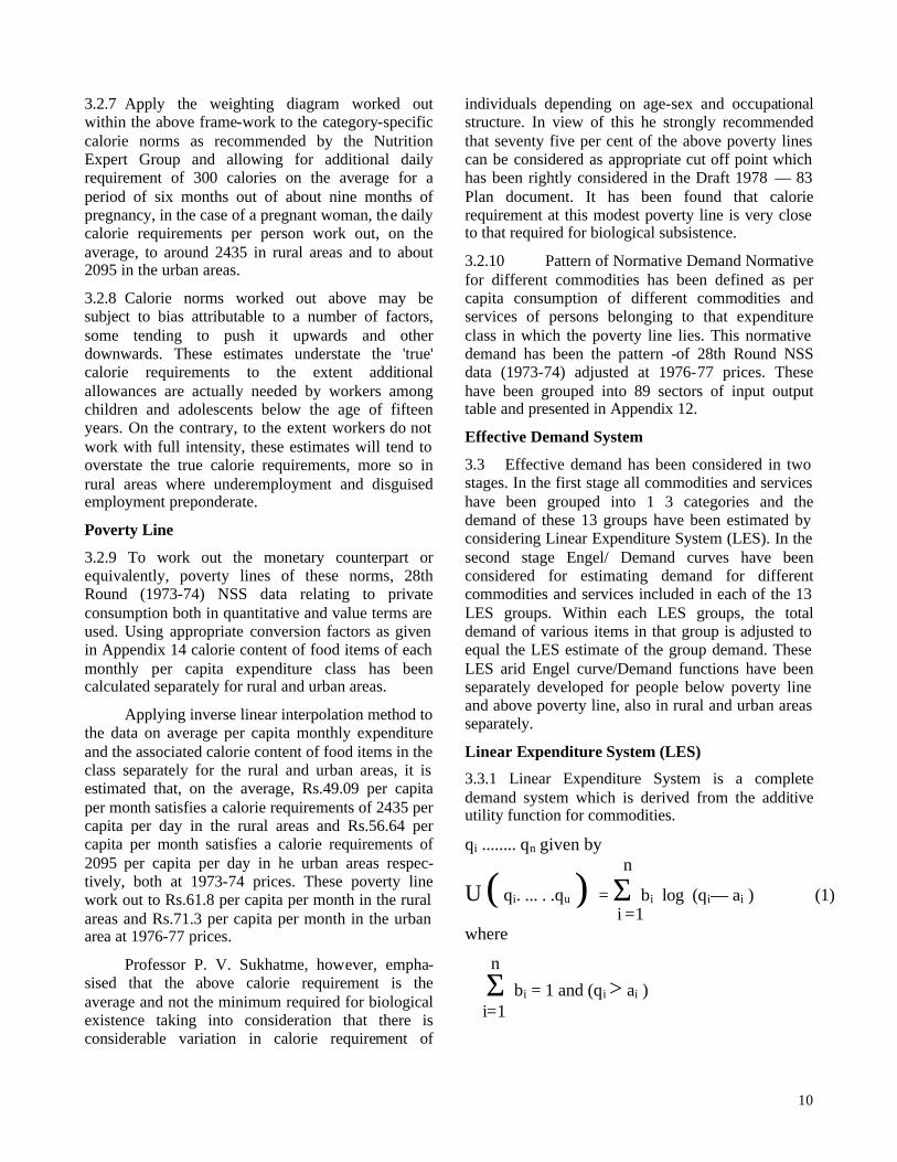
3.3.1 Linear Expenditure System is a complete demand system which is derived from the additive utility function for commodities.

qi ........ qn given by n

U ( qi. ... . .qu ) = Σ bi log (qi— ai ) (1) i =1 where

n

Σ bi = 1 and (qi > ai ) i=1

11

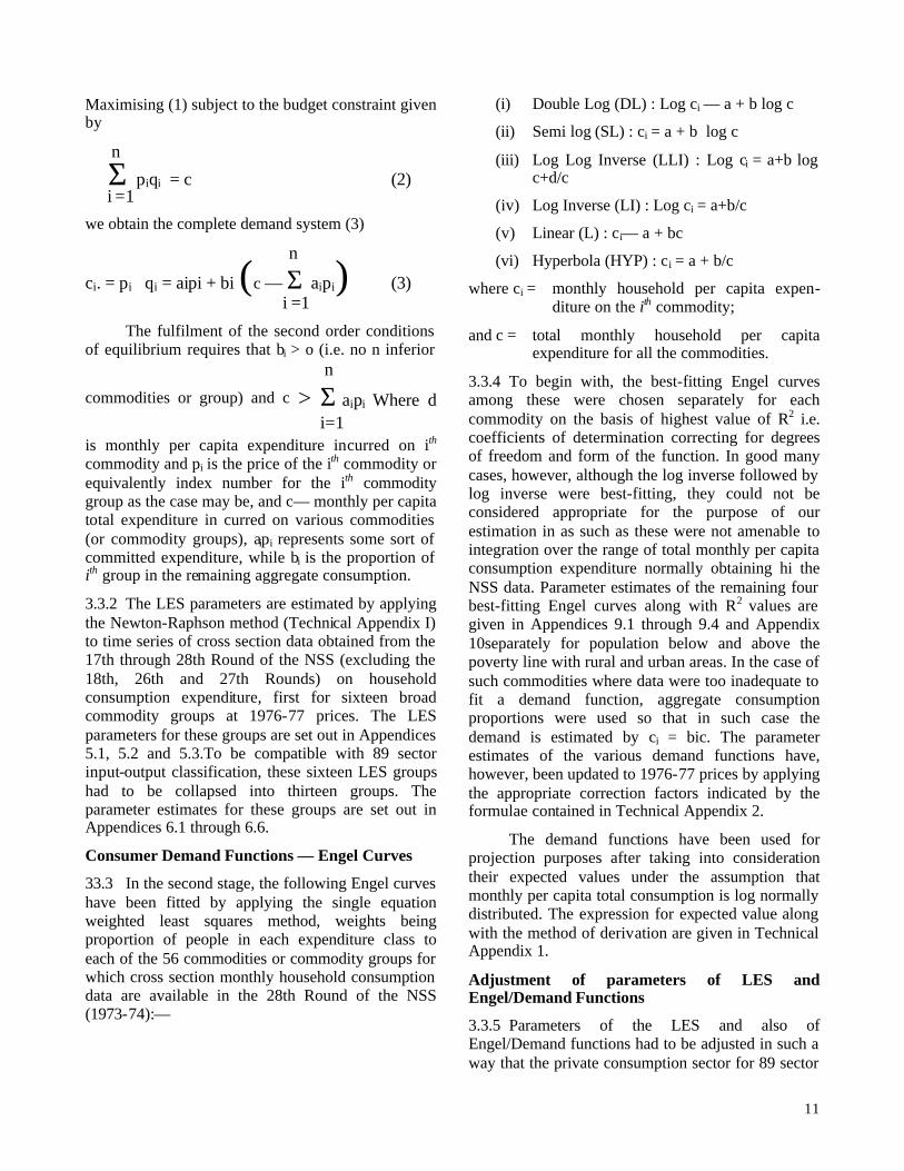
Maximising (1) subject to the budget constraint given by

n

Σ piqi = c (2) i =1

we obtain the complete demand system (3)

n

ci. = pi qi = aipi + bi (c — Σ aipi) (3) i =1

The fulfilment of the second order conditions of equilibrium requires that bi > o (i.e. no n inferior n

commodities or group) and c > Σ aipi Where d

i=1 is monthly per capita expenditure incurred on ith commodity and pi is the price of the ith commodity or equivalently index number for the ith commodity group as the case may be, and c— monthly per capita total expenditure in curred on various commodities (or commodity groups), aipi represents some sort of committed expenditure, while bi is the proportion of ith group in the remaining aggregate consumption.

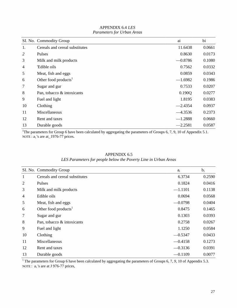
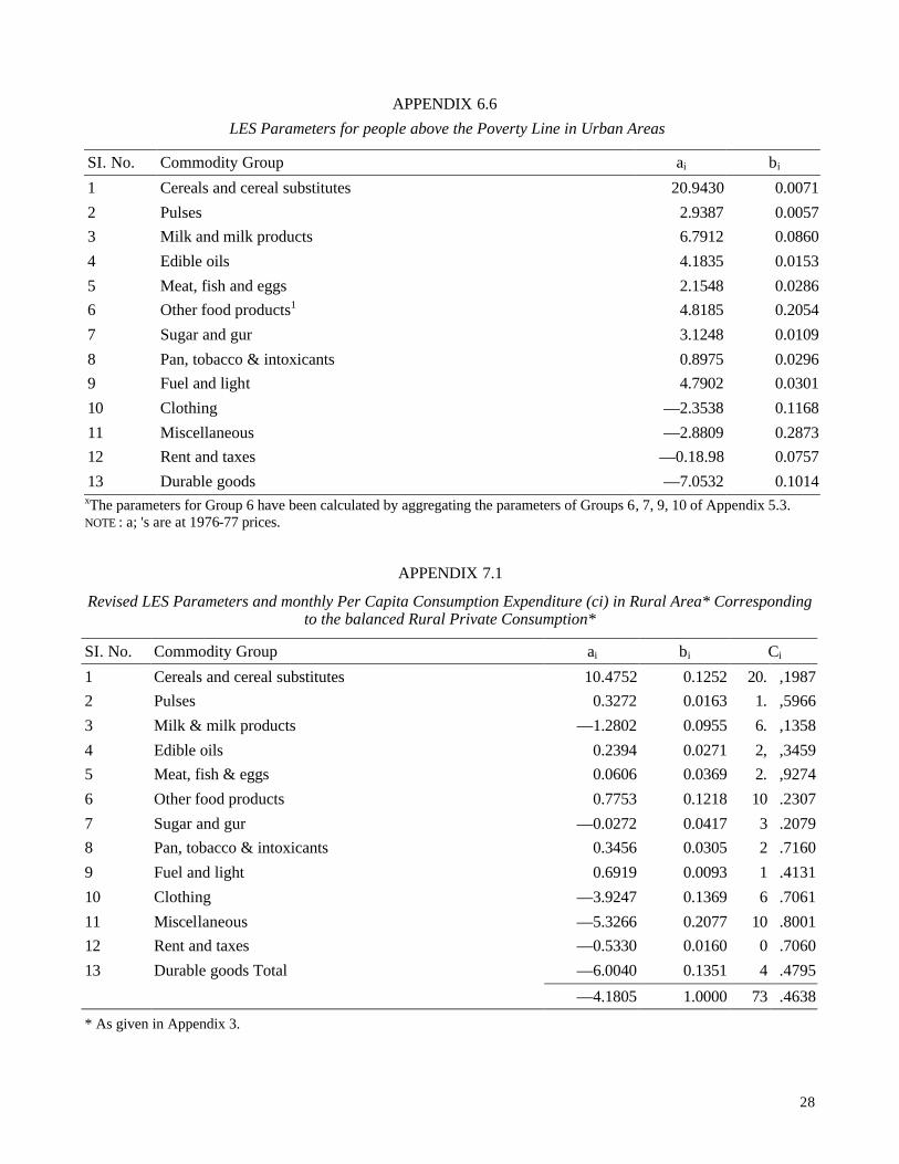
3.3.2 The LES parameters are estimated by applying the Newton-Raphson method (Technical Appendix I) to time series of cross section data obtained from the 17th through 28th Round of the NSS (excluding the 18th, 26th and 27th Rounds) on household consumption expenditure, first for sixteen broad commodity groups at 1976-77 prices. The LES parameters for these groups are set out in Appendices 5.1, 5.2 and 5.3.To be compatible with 89 sector input-output classification, these sixteen LES groups had to be collapsed into thirteen groups. The parameter estimates for these groups are set out in Appendices 6.1 through 6.6.

Consumer Demand Functions — Engel Curves

33.3 In the second stage, the following Engel curves have been fitted by applying the single equation weighted least squares method, weights being proportion of people in each expenditure class to each of the 56 commodities or commodity groups for which cross section monthly household consumption data are available in the 28th Round of the NSS (1973-74):—

(i) Double Log (DL) : Log ci — a + b log c

(ii) Semi log (SL) : ci = a + b log c

(iii) Log Log Inverse (LLI) : Log ci = a+b log c+d/c

(iv) Log Inverse (LI) : Log ci = a+b/c

(v) Linear (L) : ci— a + bc

(vi) Hyperbola (HYP) : ci = a + b/c

where ci = monthly household per capita expen-diture on the ith commodity;

and c = total monthly household per capita expenditure for all the commodities.

3.3.4 To begin with, the best-fitting Engel curves among these were chosen separately for each commodity on the basis of highest value of R2 i.e. coefficients of determination correcting for degrees of freedom and form of the function. In good many cases, however, although the log inverse followed by log inverse were best-fitting, they could not be considered appropriate for the purpose of our estimation in as such as these were not amenable to integration over the range of total monthly per capita consumption expenditure normally obtaining hi the NSS data. Parameter estimates of the remaining four best-fitting Engel curves along with R2 values are given in Appendices 9.1 through 9.4 and Appendix 10separately for population below and above the poverty line with rural and urban areas. In the case of such commodities where data were too inadequate to fit a demand function, aggregate consumption proportions were used so that in such case the demand is estimated by ci = bic. The parameter estimates of the various demand functions have, however, been updated to 1976-77 prices by applying the appropriate correction factors indicated by the formulae contained in Technical Appendix 2.

The demand functions have been used for projection purposes after taking into consideration their expected values under the assumption that monthly per capita total consumption is log normally distributed. The expression for expected value along with the method of derivation are given in Technical Appendix 1.

Adjustment of parameters of LES and Engel/Demand Functions

3.3.5 Parameters of the LES and also of Engel/Demand functions had to be adjusted in such a way that the private consumption sector for 89 sector

12

input-output table of base year, 1977-78 at 1976-77 prices generated by these functions agree with that independently estimated commodity flow approach. The procedure adopted is briefly as follows: —

(i) The aggregate private consumption for the base year i.e.1973-74, is first broken up into rural and urban components, and then into two parts, for people below poverty line and for people above poverty line by assuming that monthly per capita private consumption in 1977-78 is log normally distributed with the same inequality parameter as given by the NSS data for 1973-74.

(ii) Using the monthly per capita total consumption obtained as in step (i), in the appropriate LES demand function, the IES estimate of the total private consumption for the thirteen groups is estimated.

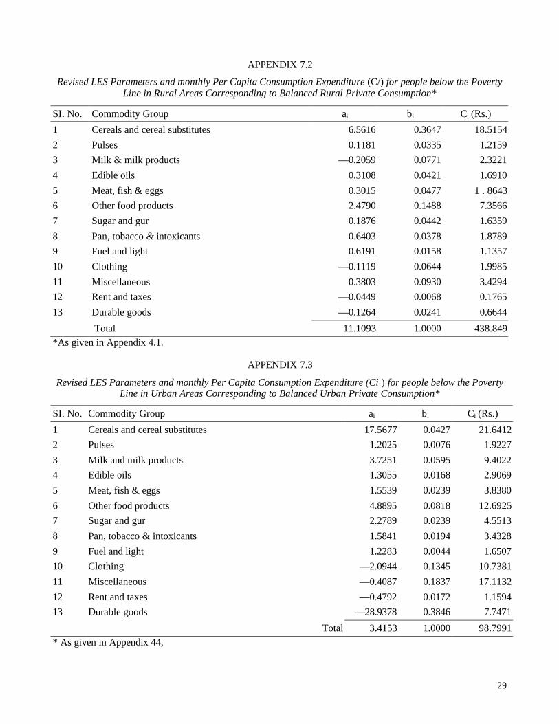
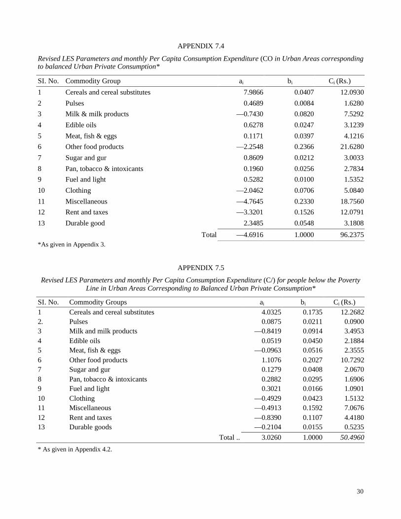
The estimates of private consumption of various commodities and services belonging to each LES group are then estimated by their respective demand functions, and then these estimates have been prorata adjusted to the corresponding LES total. The commodity-wise estimates of private consumption has then been grouped into 89 sectors of the input-output table. These sectoral estimates of private consumption are then compared with those estimated by commodity flow method and suitably adjusted in such a way that percentage difference of two sets of estimates does not generally exceed 10 to 15 per cent. The private consumption vector of 89 sectors thus obtained is used for the base year input-output table and also for adjusting the parameters of LES and demand functions. For this purpose the private consumption of 89 sectors are first aggregated to 13 LES groups. Taking these final estimates of LES groups as row control, and the given rural and urban aggregated private consumption as column controls, estimates of the 13 LES groups into rural and urban consumption has been adjusted by RAS method.* Then using these rural and urban estimates their breakdown separately into lower and upper classes has been obtained in the similar way (Appendices 4.1 and 4.2).

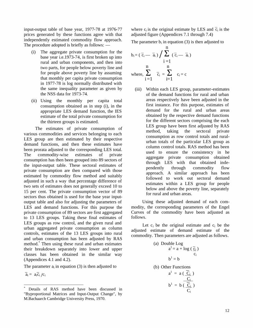
The parameter ai in equation (3) is then adjusted to

ai = aici /ci

* Details of RAS method have been discussed in "Byproportional Matrices and Input-Output Change", by M.Bachaarch Cambridge University Press, 1970.

where ci is the original estimate by LES and ci is the adjusted figure (Appendices 7.1 through 7.4)

The parameter bi in equation (3) is then adjusted to n

bi = ( ci — ai ) / Σ ( ci — ai ) i =1 n n

where, Σ ci = Σ ci = c i =1 i=1

(iii) Within each LES group, parameter-estimates of the demand functions for rural and urban areas respectively have been adjusted in the first instance. For this purpose, estimates of demand for the rural and urban areas obtained by the respective demand functions for the different sectors comprising the each LES group have been first adjusted by RAS method, taking the sectoral private consumption as row control totals and rural-urban totals of the particular LES group as column control totals. RAS method has been used to ensure the consistency in he aggregate private consumption obtained through LES with that obtained inde-pendently through commodity flow approach. A similar approach has been followed to work out sectoral demand estimates within a LES group for people below and above the poverty line, separately for rural and urban areas.

Using these adjusted demand of each com-modity, the corresponding parameters of the Engel Curves of the commodity have been adjusted as follows.

Let ci be the original estimate and ci be the adjusted estimate of demand estimate of the commodity. Then parameters are adjusted as follows.

(a) Double Log a1 = a + log ( ci ) ci b1 = b

(b) Other Functions

a1 = a ( Ci ) Ci .

b1 = b ( Ci ) Ci

13

CHAPTER 4

PROJECTION OF PRIVATE CONSUMPTION. BY INPUT-OUTPUT SECTORS

This chapter outlines procedure adopted to estimate the private consumption demand for the 89 sectors of the input-output model considered for the terminal year (1982-83) of the 6th Five Year Plan period, as well as for the terminal year (1987-88) of the perspective Period. Keeping in view the plan objective of reduction of poverty during the period, two alternative assumptions have been considered for the purpose. These are: —

1. All people below the poverty line may be raised to the poverty line and would have the pattern of consumption according to the normative sectoral demand. This will be termed as Variant I.

2. In the second alternative case, all people below the 75 per cent of poverty line (to be called modest poverty line) would have at least the modest poverty line consumption. It has been assumed that in the process of redistribution the average consumption for people between modest poverty line and poverty line remains the same as before redistribution of the people between modest poverty line ad the poverty line. In this case the private consumption of the people below the poverty line would be estimated by considering the effective demand system developed for people below poverty line. This will be termed as Variant II.

4.1.1. In both variants the private consumption available after meeting the demand for people below the poverty line would be assumed to be consumed by people above the poverty line, the sectoral demand of which will be estimated by the effective demand system developed for this class of population.

4.1.2. The variant II was also considered by assuming modest poverty line to be more than 75 per cent of the poverty line. But such cases were not found to be feasible due to supply constraints on some critical items like foodgrains.

4.2. The procedure adopted for estimating the private consumption vector in above two variants is discussed below: —

(i) The aggregate private consumption obtained from macro-economic projections through a macro-model is first divided into rural and urban components by using an independently estimated value of ratio of the per capita consumption in the urban area to that in the rural area. This ratio is based upon past data of NSS as well as the policy consideration that rural per capita income would grow faster than urban per capita income.

Following relations have been used for this purpose.

C = Cr + Cu ...........................................(1)

Vr = Cr/12Pr ...........................................(2)

Vu = Cu/12Pu ...........................................(3)

Vu = bVr ...........................................(4)

where

C = total private consumption as given by the macro model;

Cr = total private consumption in rural areas;

Cu = total private consumption in urban areas;

Vr = monthly per capita total private consumption in rural areas;

Vu = monthly per capita total private consumption in urban areas;

Pr = population in rural areas;

Pu = population in urban areas; and

b = estimate of ratio of per capita consumption in urban areas to that in rural areas.

Table 1 presents values of b, Pr, Pu, Vr & Vu in different time periods.

14

TABLE 1

Year b C Rs. in million Pr million Pu million Vr Rs. Vu Rs. 1977-78 1.31 591070 495.2 133.8 73.46 96.24 1982-83 1.26 729430 537.2 154.8 83.01 104.60 1987-88 1.24 932810 577.7 177.5 97.44 120.82

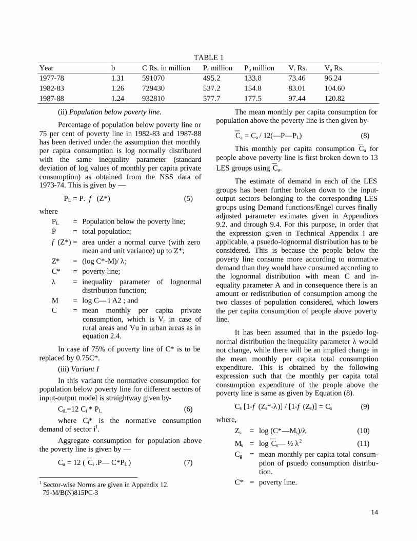
(ii) Population below poverty line.

Percentage of population below poverty line or 75 per cent of poverty line in 1982-83 and 1987-88 has been derived under the assumption that monthly per capita consumption is log normally distributed with the same inequality parameter (standard deviation of log values of monthly per capita private consumption) as obtained from the NSS data of 1973-74. This is given by —

PL = P. φ (Z*) (5)

where PL = Population below the poverty line; P = total population;

φ (Z*) = area under a normal curve (with zero mean and unit variance) up to Z*;

Z* = (log C*-M)/ λ; C* = poverty line;

λ = inequality parameter of lognormal distribution function;

M = log C— i A2 ; and C = mean monthly per capita private

consumption, which is Vr in case of rural areas and Vu in urban areas as in equation 2.4.

In case of 75% of poverty line of C* is to be replaced by 0.75C*.

(iii) Variant I

In this variant the normative consumption for population below poverty line for different sectors of input-output model is straightway given by-

CiL=12 Ci * PL (6)

where Ci* is the normative consumption demand of sector i1.

Aggregate consumption for population above the poverty line is given by —

Ca = 12 ( Ci .P— C*PL ) (7)

1 Sector-wise Norms are given in Appendix 12. 79-M/B(N)815PC-3

The mean monthly per capita consumption for population above the poverty line is then given by-

Ca = Ca / 12(—P—PL) (8)

This monthly per capita consumption Ca for people above poverty line is first broken down to 13

LES groups using Ca.

The estimate of demand in each of the LES groups has been further broken down to the input-output sectors belonging to the corresponding LES groups using Demand functions/Engel curves finally adjusted parameter estimates given in Appendices 9.2. and through 9.4. For this purpose, in order that the expression given in Technical Appendix I are applicable, a psuedo-lognormal distribution has to be considered. This is because the people below the poverty line consume more according to normative demand than they would have consumed according to the lognormal distribution with mean C and in-equality parameter A and in consequence there is an amount or redistribution of consumption among the two classes of population considered, which lowers the per capita consumption of people above poverty line.

It has been assumed that in the psuedo log-normal distribution the inequality parameter λ would not change, while there will be an implied change in the mean monthly per capita total consumption expenditure. This is obtained by the following expression such that the monthly per capita total consumption expenditure of the people above the poverty line is same as given by Equation (8).

Cs [1-φ (Zs*-λ)] / [1-φ (Zs)] = Ca (9)

where,

Zs = log (C*—Ms)/λ (10)

Ms = log Cs— ½ λ2 (11)

Cg = mean monthly per capita total consum-ption of psuedo consumption distribu-tion.

C* = poverty line.

15

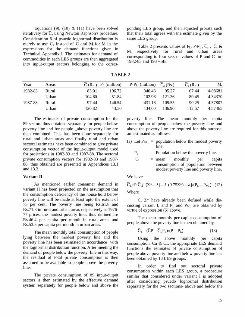
Equations (9), (10) & (11) have been solved iteratively for Ca using Newton Raphson's procedure. Consideration δ of psuedo lognormal distribution is merely to use Ca instead of C and Ms for M in the expressions for the demand functions given in Technical Appendix I. The estimates for demand of commodities in each LES groups are then aggregated into input-output sectors belonging to the corres-

ponding LES group, and then adjusted prorata such that their total agrees with the estimate given by the same LES group.

Table 2 presents values of PL, P-PL , Ca , Cs & Ms respectively for rural and urban areas corresponding to four sets of values of P and C for 1982-83 and 198 /-SB.

TABLE 2

Year Areas C (Rs.) PL (million) P-PL (million) Ca (Rs.) Cs (Rs.) Ms

1982-83 Rural 83.01 196.72 340.48 95.27 67.44 4-08681 Urban 104.60 51.84 102.96 121.36 89.45 4.34370 1987-88 Rural 97.44 146.54 431.16 109.55 90.25 4.37807 Urban 120.82 43.50 134.00 136.90 112.67 4.57465

The estimates of private consumption for the 89 sectors thus obtained separately for people below poverty line and for people _above poverty line are then combined. This has been done separately for rural and urban areas and finally rural and urban sectoral estimates have been combined to give private consumption vector of the input-output model used for projections in 1982-83 and 1987-88. The sectoral private consumption vectors for 1982-83 and 1987-88, thus obtained are presented in Appendices 13.1 and 13.2.

Variant II

As mentioned earlier consumer demand in variant II has been projected on the assumption that the consumption deficiency of the house hold below poverty line will be made at least upto the extent of 75 per cent. The poverty line being Rs.61.8 and Rs.71.3 in rural and urban areas respectively at 1976-77 prices, the modest poverty lines thus defined are Rs.46.4 per capita per month in rural areas and Rs.53.5 per capita per month in urban areas.

The mean monthly total consumption of people lying between the modest poverty line and the poverty line has been estimated in accordance with the lognormal distribution function. After meeting the demand of people below the poverty line in this way, the residual of total private consumption is then assumed to be available to people above the poverty line.

The private consumption of 89 input-output sectors is then estimated by the effective demand system separately for people below and above the

poverty line. The mean monthly per capita consumption of people below the poverty line and above the poverty line are required for this purpose are estimated as follows:—

(a) Let PML = population below the modest poverty line.

PL = Population below the poverty line.

CL = mean monthly per capita consumption of population between modest poverty line and poverty line,

We have

CL=P.C[φ (Ζ*—λ)—φ (0.75Z*)—λ]/(PL—PML) (12)

Where

C, Z* have already been defined while dis-cussing variant I, and PL and PML are obtained by virtue of expression (5) above.

The mean monthly per capita consumption of people above the poverty line is then obtained by-

Ca = (CP—CLPL)/(P—PL) (13)

Using the above monthly per capita consumption, Ca & CL the appropriate LES demand functions the estimates of private consumption of people above poverty line and below poverty line has been obtained by 13 LES groups.

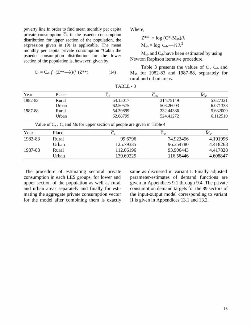
In order to find out sectoral private consumption within each LES group, a procedure similar that considered under variant I is adopted after considering psuedo lognormal distribution separately for the two sections- above and below the

16

poverty line In order to find mean monthly per capita private consumption Cs in the psuedo consumption distribution for upper section of the population, the expression given in (9) is applicable. The mean monthly per capita private consumption "Cabin the psuedo consumption distribution for the lower section of the population is, however, given by.

CL = Csb φ (Ζ**—λ)/φ (Z**) (14)

Where,

Z** = log (C*-Msb)/λ

Msb = log Csb —½ λ2

Msb and Csb have been estimated by using Newton Raphson iterative procedure.

Table 3 presents the values of Cb, Csb and Msb for 1982-83 and 1987-88, separately for rural and urban areas.

TABLE - 3

Year Place Cb Csb Msb 1982-83 Rural 54.15017 314.75149 5.627321 Urban 62.50575 503.26003 6.071338 1987-88 Rural 54.39899 332.44386 5.682000 Urban 62.68799 524.41272 6.112510

Value of Ca , Cs and Ms for upper section of people are given in Table 4

Year Place Ca Csb Msb 1982-83 Rural 99.6796 74.923456 4.191996 Urban 125.79335 96.354780 4.418268 1987-88 Rural 112.06196 93.906443 4.417828 Urban 139.69225 116.58446 4.608847

The procedure of estimating sectoral private consumption in each LES groups, for lower and upper section of the population as well as rural and urban areas separately and finally for esti-mating the aggregate private consumption vector for the model after combining them is exactly

same as discussed in variant I. Finally adjusted parameter-estimates of demand functions are given in Appendices 9.1 through 9.4. The private consumption demand targets for the 89 sectors of the input-output model corresponding to variant II is given in Appendices 13.1 and 13.2.

17

CHAPTER 5

RECOMMENDATIONS AND FUTURE DIRECTION OF WORK

Recommendation

During the course of discussions, the Task Force suggested the following recommendations:—

(a) To estimate the average calorie requirement for an individual separately for rural and urban areas taking into consideration the distribution of age, sex and activity.

(b) To estimate the poverty line corresponding to the calorie requirement using the NSS data of the 28th round (1973-74).

(c) To estimate commodity-wise private consumption effective/ behaviouristic and normative for the Sixth Plan 1978 — 83. It was recommended that the commodity-wise private consumption may be estimated by considering linear expenditure system (LES) for maximum number of groups of commodities and best fitting Engel curves within each LES group.

The Committee further recommended that the views expressed by Prof. N.S. lyengar in his letter to the convenor and there actions of Dr. R. Radha krishna be appended to the Report.

(d) As for calculating the calorie requirement, it is preferable to consider the minimum rather than average required for biological existence taking into consideration that there is considerable variation in calorie requirement. In view of this, it is recommended that 75 per cent of the poverty line may be considered as appropriate cut off point which has been rightly considered in the Draft 1978—83 Plan document.

Future Directions of Work

5.2. It was agreed that the following aspects may be taken up as tasks ahead for estimating the private consumption vector of the input-output model. These are:-

(i) Methodological framework of consumption model;

(ii) Concomitant data problems; and

(iii) Related operational issues.

5.3. Methodological Framework

This relates to normative as well as effective/ behaviouristic and other alternative aspects of the consumption model.

(i) Normative Consumption

5.3.1. In constructing the weighting diagram for determining the all-India calorie requirements separately for rural and urban areas, certain as-sumptions have been made. In this connection, it seems useful from operational angle to firm up some of these, particularly the one related to classification of workers as heavy, moderate and sedentary. To this end, a quick survey of existing literature on the subject, coupled with some exercises based on available data, may commend.

5.3.2. Since daily calorie requirements for the same person category are likely to vary over space because of climatic factors difference in body weights, etc., it appears desirable, at least in the long run, to develop regional calorie norms. Regions having formed, as much as possible, on the basis of homogeneity criterion consistent with similarity of climatic factors, uniformity of body weights, etc. As a corollary to this, a refinement to the procedure adopted at present to work out all-India calorie requirements seems in order. First over all region-level calorie requirements will have to be worked out and then an all-India figure arrived at by weighting these regional figures; the weights being the regional population figures.

5.3.3. A comparison of two series of private consumption expenditure one based on NSS household consumption expenditure-data and the other brought out by the CSO as a part of their National Accounts Statistics — shows that they differ perceptibly with the NSS series invariably tending to be on the low side. The reasons behind these differences and how to reconcile, them is obviously a matter for further research and investigation. In this connection, it may be added that if, for instance, in actuality food items are correctly reported and non-food items alone are under-reported, then evidently, poverty line as calculated by us is understated and so also the population below it. On the contrary, converse holds good if non-food items are correctly reported and food items are under-reported.

18

5.3.4. Food component of the poverty line could alternatively be obtained by L P model** resulting in a minimum cost balanced diet compatible with locally available food-stuffs and satisfying, as far as possible, local tastes and preferences. Minimum cost figures thus arrived at for various person categories could be aggregated into an overall region-level or all-India figure by using an appropriate weighting diagram. This, when added to the food component of the original poverty line, would result in an alternative poverty line estimate. This may be more realistic via-a-vis the original poverty line inasmuch as its food component is based on observational data rather than interview-based data which, in no small measure, may be affected by various biases and errors attributable to this method. In fact, norms for non-food component could also be suitably modified and moderated in the light of the observations made by various distinguished study groups in connection with their recommendations on minimum wage or need-based wage, etc., and allied materials available on the subject as well as through independent studies.

Effective Consumption

5.3.5. Effective/ behaviouristic demand in the present work has been analysed within the framework of L E S-cum-consumption functions model. In the ensuring discussion we will take up the LES followed by its integration with demand functions.

5.3.6. Leaving aside the limitations of the LES to satisfactorily handle price effects-cross as well as own-pragmatic considerations suggest that certain modifications could be introduced in it while largely retaining its original structure and simplicity to allow greater sophistication in income response. The simplest way to achieve it is, as already tried out by some researchers in the field, to introduce time trends in the LES parameters preferably in this only, to allow for steady changes in tastes and preferences.

5.3.7. To judge the relative performance of LES, it may be instructive to compare its results with those of alternative models.

5.3.8. The consumption model for demand projections is intended to capture essentially the inter-temporal variations in consumer behaviour which is essentially of a short-run nature. As against this parameter of LES estimated in the present work tend to be a 'mongrel' reflecting both the short-term * Some work in this area as a part of district level food and nutrition studies is being undertaken by Department of Food.

and long-term consumption behaviours. This is because the time series- of cross section data used in the model not only include inter-temporal variations but inter-cross section variations also. Inter-temporal variations could probably be disentangled by using dummy variables for cross sections in the regression analysis.

Problem of Integration 5.3.9. Integration of demand functions with LES

tantamounts to assuming that both the systems reflect the same behaviour pattern of the consumer. But, as is well known, cross section analysis relating to a single point of time essentially reflects long-term consumption behaviour. In a situation like this, it may be argued whether integration is at all warranted. A way out of these theoretical complications relating to specification and interpretation of the model, of course within the LES framework, may be to estimate LES on the basis of regression analysis using dummy variables applied to time series of cross section data on the one hand and estimating demand functions on time series data for finer classification of broad consumption estimates yielded by the LES on the other hand. As far as the latter is concerned, this will necessitate availability of house-hold consumption data in as much detail as contained in 28th Round of the NSS for a series of rounds.

(ii) Data

5.4.1. Natonal Sample Survey household con-sumption data are collected, both in value and quantity wherever relevant, at a fairly disaggregative level. In order that the data may be useful for the purpose of consumption model building, they should also be available both for the previous rounds and for the up-coming rounds in as detailed a manner as is the case with the 28th round of the NSS. In the case of States, in order to get tolerably realistic estimation of the model, the relevant tabulations would have to be based on Central sample data and State sample data combined to overcome the problem of small sample size. Wherever State sample is not collected, the same would have to be collected in future or Central sample would have to be of adequate size. As regards index number problem, the implicit deflator, if worked out regularly, based on National Sample Survey value and quantity data would probably resolve it. In the case of such items where only value figures are available, appropriate unit prices will also have to be collected or compiled.

19

5.4.2. Closer examination and scrutiny of concepts, definitions, coverage and related aspects ' needs no emphasis to throw light on the disparity between the NSS and CSO series of private consumption expenditure. In this connection, surveys like Food and Nutrition studies being conducted by Food and Nutrition Board, Ministry of Agriculture and Irrigation, Department of Food, could provide an independent check on the two sets of data in question.

(iii) Related Operational Issues

5.5. This section broadly recapitulates area of further work: —

i) Preparation of a paper surveying the existing literature on consumption functions and demand projections;

ii) Discussion regarding the norms that should be adopted in respect of non-traded public goods like housing, primary education, drinking water and medicines. In this connection, Appendices 15.1 & 15.2 give certain norms and coefficients. This information has been gleaned from a recent note entitled 'Minimum Needs Programme and its Commodity Composition', prepared by the Perspective Planning Division;

iii) Views should be expressed on the distribution policy that should be adopted regarding food, sugar, clothing, housing, education, health and miscellaneous civil services in the final report;

iv) Regional focus in the estimation of demand for various essential commodities should be brought out; and

v) For estimation of private consumption : for the new plan model, studies comprising the following should be carried out: —

(a) re-estimation of the linear expenditure system considering more number of commodity groups preferably comparable with the input-output classification using the latest NSS data,

(b) estimation of linear expenditure system for different groups of expenditure classes taking into consideration the change in the expenditure classes over different rounds due to price changes,

(c) estimation of different Engle curves for as many number of commodities as possible using data of various NSS Rounds, and

(d) estimation of regional specific norms of minimum needs both for essential traded goods and non-traded public goods, and

(e) consideration of alternative consumption model.

Sd/- Dr. Y. K. Alag Adviser (PP), Planning Commission.

Sd/- Shri D. Goondoo, Economic Research Unit, Indian Statistical Institute, 203, Barrackpore Trunk Road, Calcutta-700035.

Sd/- Dir. D.B. Gupta, Institute of Economic Growth, University Enclave, Delhi-110007.

Sd/- Prof. N.S. lyengar, Department of Economics, Osmania University, Hyderabad-500007;

Sd/- Dr. L.R. Jain, Indian Statistical Institute, 7, SJ.S. Sensanwal Marg, New Delhi-110029.

Sd/- Shri G.V.S.N. Murty, Sardar Patel Institute of Economic & Social Research, Navrangpura, Ahmedabad-380009.

Sd/- Prof. R, Radhakrishna, Sardar Patel Institute of Economic & Social Research, Navrangpura, Ahmedabad-380009.

20

Sd/- Prof. P.V. Sukhatme, Maharashtra Association for Cultivation, Poona-4.

Sd/- Dr. S.D. Tandulkar, Indian Statistical Institute 7, S.J.S. Sansanwal Marg,

New Delhi-110002.

Sd/- Dr. K.C. Majumdar, Jt. Adviser (PP), Planning Commission.

21

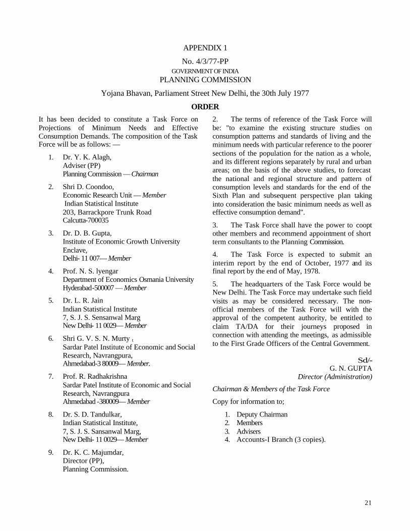
APPENDIX 1

No. 4/3/77-PP GOVERNMENT OF INDIA

PLANNING COMMISSION

Yojana Bhavan, Parliament Street New Delhi, the 30th July 1977

ORDER

It has been decided to constitute a Task Force on Projections of Minimum Needs and Effective Consumption Demands. The composition of the Task Force will be as follows: —

1. Dr. Y. K. Alagh, Adviser (PP) Planning Commission — Chairman

2. Shri D. Coondoo, Economic Research Unit — Member Indian Statistical Institute 203, Barrackpore Trunk Road Calcutta-700035

3. Dr. D. B. Gupta, Institute of Economic Growth University Enclave, Delhi- 11 007— Member

4. Prof. N. S. lyengar Department of Economics Osmania University Hyderabad-500007 — Member

5. Dr. L. R. Jain Indian Statistical Institute 7, S. J. S. Sensanwal Marg New Delhi- 11 0029— Member

6. Shri G. V. S. N. Murty t Sardar Patel Institute of Economic and Social Research, Navrangpura, Ahmedabad-3 80009— Member.

7. Prof. R. Radhakrishna Sardar Patel Institute of Economic and Social Research, Navrangpura Ahmedabad -380009— Member

8. Dr. S. D. Tandulkar, Indian Statistical Institute, 7, S. J. S. Sansanwal Marg, New Delhi- 11 0029— Member

9. Dr. K. C. Majumdar, Director (PP), Planning Commission.

2. The terms of reference of the Task Force will be: "to examine the existing structure studies on consumption patterns and standards of living and the minimum needs with particular reference to the poorer sections of the population for the nation as a whole, and its different regions separately by rural and urban areas; on the basis of the above studies, to forecast the national and regional structure and pattern of consumption levels and standards for the end of the Sixth Plan and subsequent perspective plan taking into consideration the basic minimum needs as well as effective consumption demand".

3. The Task Force shall have the power to coopt other members and recommend appointment of short term consultants to the Planning Commission.

4. The Task Force is expected to submit an interim report by the end of October, 1977 and its final report by the end of May, 1978.

5. The headquarters of the Task Force would be New Delhi. The Task Force may undertake such field visits as may be considered necessary. The non-official members of the Task Force will with the approval of the competent authority, be entitled to claim TA/DA for their journeys proposed in connection with attending the meetings, as admissible to the First Grade Officers of the Central Government.

Sd/- G. N. GUPTA

Director (Administration)

Chairman & Members of the Task Force

Copy for information to;

1. Deputy Chairman 2. Members 3. Advisers 4. Accounts-I Branch (3 copies).

22

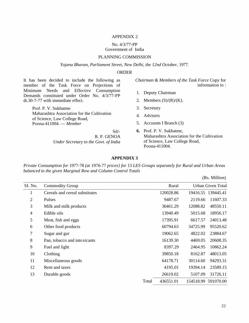
APPENDIX 2

No. 4/3/77-PP Government of India

PLANNING COMMISSION

Yojana Bhavan, Parliament Street, New Delhi, the 12nd October, 1977.

ORDER

It has been decided to include the following as member of the Task Force on Projections of Minimum Needs and Effective Consumption Demands constituted under Order No. 4/3/77-PP dt.30-7-77 with immediate effect.

Prof. P. V. Sukhatme Maharashtra Association for the Cultivation of Science, Law College Road, Poona-411004. — Member

Sd/- R. P. GENOA

Under Secretary to the Govt. of India

Chairman & Members of the Task Force Copy for information to :

1. Deputy Chairman

2. Members (S)/(R)/(K).

3. Secretary

4. Advisers

5. Accounts I Branch (3)

6. Prof. P. V. Sukhatme, Maharashtra Association for the Cultivation of Science, Law College Road, Poona-411004.

APPENDIX 3

Private Consumption for 1977-78 (at 1976-77 prices} for 13 LES Groups separately for Rural and Urban Areas balanced to the given Marginal Row and Column Control Totals

(Rs. Million)

SI. No. Commodity Group Rural Urban Given Total

1 Cereals and cereal substitutes 120028.86 19416.55 139445.41

2 Pulses 9487.67 2119.66 11607.33

3 Milk and milk products 36461.29 12088.82 48550.11

4 Edible oils 13940.49 5015.68 18956.17

5 Meat, fish and eggs 17395.91 6617.57 24013.48

6 Other food products 60794.63 34725.99 95520.62

7 Sugar and gur 19062.65 4822.02 23884.67

8 Pan, tobacco and intoxicants 16139.30 4469.05 20608.35

9 Fuel and light 8397.29 2464.95 10862.24

10 Clothing 39850.18 8162.87 48013.05

11 Miscellaneous goods 64178.71 30114.60 94293.31

12 Rent and taxes 4195.01 19394.14 23589.15

26619.02 5107.09 31726.11 13 Durable goods

Total 436551.01 154518.99 591070.00

23

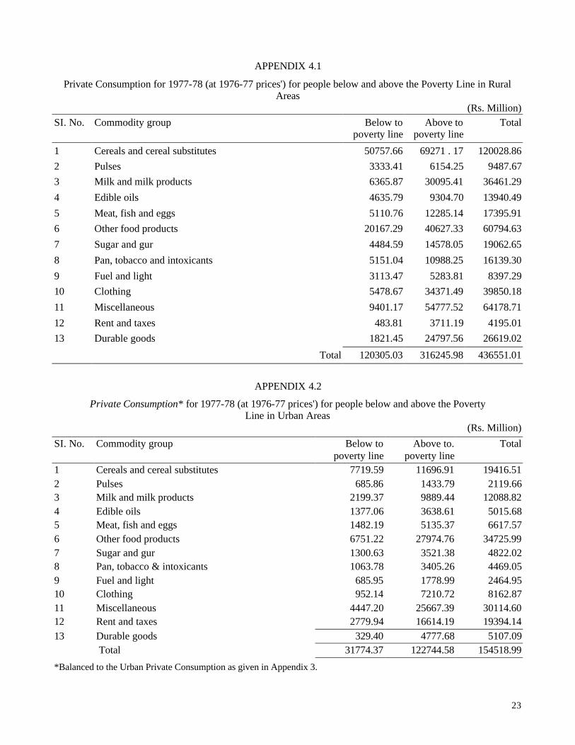
APPENDIX 4.1

Private Consumption for 1977-78 (at 1976-77 prices') for people below and above the Poverty Line in Rural Areas

(Rs. Million)

SI. No. Commodity group Below to poverty line

Above to poverty line

Total

1 Cereals and cereal substitutes 50757.66 69271 . 17 120028.86

2 Pulses 3333.41 6154.25 9487.67


4 Edible oils 4635.79 9304.70 13940.49

5 Meat, fish and eggs 5110.76 12285.14 17395.91


7 Sugar and gur 4484.59 14578.05 19062.65

8 Pan, tobacco and intoxicants 5151.04 10988.25 16139.30

9 Fuel and light 3113.47 5283.81 8397.29

10 Clothing 5478.67 34371.49 39850.18

11 Miscellaneous 9401.17 54777.52 64178.71

12 Rent and taxes 483.81 3711.19 4195.01

13 Durable goods 1821.45 24797.56 26619.02

Total 120305.03 316245.98 436551.01

APPENDIX 4.2

Private Consumption* for 1977-78 (at 1976-77 prices') for people below and above the Poverty Line in Urban Areas

(Rs. Million)

SI. No. Commodity group Below to poverty line

Above to. poverty line

Total

1 Cereals and cereal substitutes 7719.59 11696.91 19416.51 2 Pulses 685.86 1433.79 2119.66 3 Milk and milk products 2199.37 9889.44 12088.82 4 Edible oils 1377.06 3638.61 5015.68 5 Meat, fish and eggs 1482.19 5135.37 6617.57 6 Other food products 6751.22 27974.76 34725.99 7 Sugar and gur 1300.63 3521.38 4822.02 8 Pan, tobacco & intoxicants 1063.78 3405.26 4469.05 9 Fuel and light 685.95 1778.99 2464.95 10 Clothing 952.14 7210.72 8162.87 11 Miscellaneous 4447.20 25667.39 30114.60 12 Rent and taxes 2779.94 16614.19 19394.14

13 Durable goods 329.40 4777.68 5107.09 Total 31774.37 122744.58 154518.99

*Balanced to the Urban Private Consumption as given in Appendix 3.

24

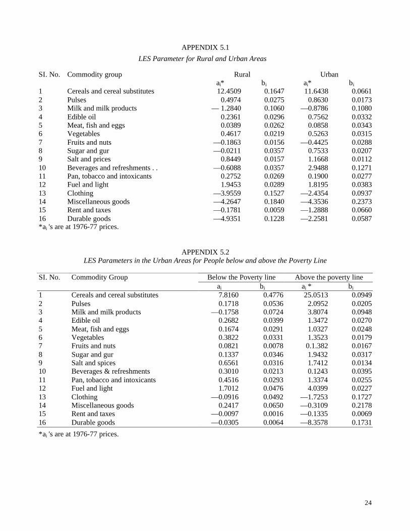
APPENDIX 5.1

LES Parameter for Rural and Urban Areas

Rural Urban SI. No. Commodity group ai* bi ai* bi

1 Cereals and cereal substitutes 12.4509 0.1647 11.6438 0.0661 2 Pulses 0.4974 0.0275 0.8630 0.0173 3 Milk and milk products — 1.2840 0.1060 —0.8786 0.1080 4 Edible oil 0.2361 0.0296 0.7562 0.0332 5 Meat, fish and eggs 0.0389 0.0262 0.0858 0.0343 6 Vegetables 0.4617 0.0219 0.5263 0.0315 7 Fruits and nuts —0.1863 0.0156 —0.4425 0.0288 8 Sugar and gur —0.0211 0.0357 0.7533 0.0207 9 Salt and prices 0.8449 0.0157 1.1668 0.0112 10 Beverages and refreshments . . —0.6088 0.0357 2.9488 0.1271 11 Pan, tobacco and intoxicants 0.2752 0.0269 0.1900 0.0277 12 Fuel and light 1.9453 0.0289 1.8195 0.0383 13 Clothing —3.9559 0.1527 —2.4354 0.0937 14 Miscellaneous goods —4.2647 0.1840 —4.3536 0.2373 15 Rent and taxes —0.1781 0.0059 —1.2888 0.0660 16 Durable goods —4.9351 0.1228 —2.2581 0.0587 *ai 's are at 1976-77 prices.

APPENDIX 5.2 LES Parameters in the Urban Areas for People below and above the Poverty Line

Below the Poverty line Above the poverty line SI. No. Commodity Group ai bi ai * bi

1 Cereals and cereal substitutes 7.8160 0.4776 25.0513 0.0949 2 Pulses 0.1718 0.0536 2.0952 0.0205 3 Milk and milk products —0.1758 0.0724 3.8074 0.0948 4 Edible oil 0.2682 0.0399 1.3472 0.0270 5 Meat, fish and eggs 0.1674 0.0291 1.0327 0.0248 6 Vegetables 0.3822 0.0331 1.3523 0.0179 7 Fruits and nuts 0.0821 0.0078 0.1.382 0.0167 8 Sugar and gur 0.1337 0.0346 1.9432 0.0317 9 Salt and spices 0.6561 0.0316 1.7412 0.0134 10 Beverages & refreshments 0.3010 0.0213 0.1243 0.0395 11 Pan, tobacco and intoxicants 0.4516 0.0293 1.3374 0.0255 12 Fuel and light 1.7012 0.0476 4.0399 0.0227 13 Clothing —0.0916 0.0492 —1.7253 0.1727 14 Miscellaneous goods 0.2417 0.0650 —0.3109 0.2178 15 Rent and taxes —0.0097 0.0016 —0.1335 0.0069 16 Durable goods —0.0305 0.0064 —8.3578 0.1731

*ai 's are at 1976-77 prices.

25

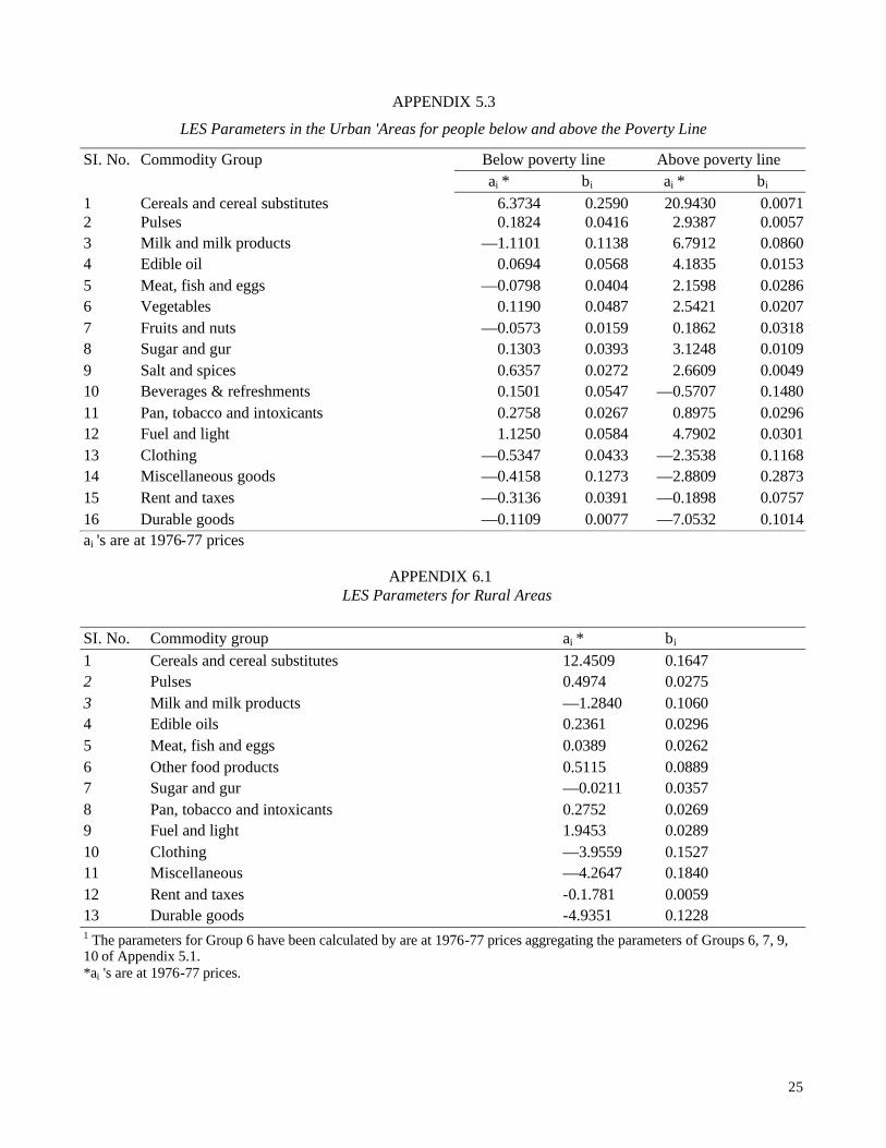
APPENDIX 5.3

LES Parameters in the Urban 'Areas for people below and above the Poverty Line

Below poverty line Above poverty line SI. No.

Commodity Group ai * bi ai * bi

1 2

Cereals and cereal substitutes Pulses

6.3734 0.1824

0.2590 0.0416

20.9430 2.9387

0.0071 0.0057

3 Milk and milk products —1.1101 0.1138 6.7912 0.0860 4 Edible oil 0.0694 0.0568 4.1835 0.0153 5 Meat, fish and eggs —0.0798 0.0404 2.1598 0.0286 6 Vegetables 0.1190 0.0487 2.5421 0.0207 7 Fruits and nuts —0.0573 0.0159 0.1862 0.0318 8 Sugar and gur 0.1303 0.0393 3.1248 0.0109 9 Salt and spices 0.6357 0.0272 2.6609 0.0049 10 Beverages & refreshments 0.1501 0.0547 —0.5707 0.1480 11 Pan, tobacco and intoxicants 0.2758 0.0267 0.8975 0.0296 12 Fuel and light 1.1250 0.0584 4.7902 0.0301 13 Clothing —0.5347 0.0433 —2.3538 0.1168 14 Miscellaneous goods —0.4158 0.1273 —2.8809 0.2873 15 Rent and taxes —0.3136 0.0391 —0.1898 0.0757 16 Durable goods —0.1109 0.0077 —7.0532 0.1014 ai 's are at 1976-77 prices

APPENDIX 6.1 LES Parameters for Rural Areas

SI. No. Commodity group ai * bi

1 Cereals and cereal substitutes 12.4509 0.1647 2 Pulses 0.4974 0.0275 3 Milk and milk products —1.2840 0.1060 4 Edible oils 0.2361 0.0296 5 Meat, fish and eggs 0.0389 0.0262 6 Other food products 0.5115 0.0889 7 Sugar and gur —0.0211 0.0357 8 Pan, tobacco and intoxicants 0.2752 0.0269 9 Fuel and light 1.9453 0.0289 10 Clothing —3.9559 0.1527 11 Miscellaneous —4.2647 0.1840 12 Rent and taxes -0.1.781 0.0059 13 Durable goods -4.9351 0.1228 1 The parameters for Group 6 have been calculated by are at 1976-77 prices aggregating the parameters of Groups 6, 7, 9, 10 of Appendix 5.1. *ai 's are at 1976-77 prices.

26

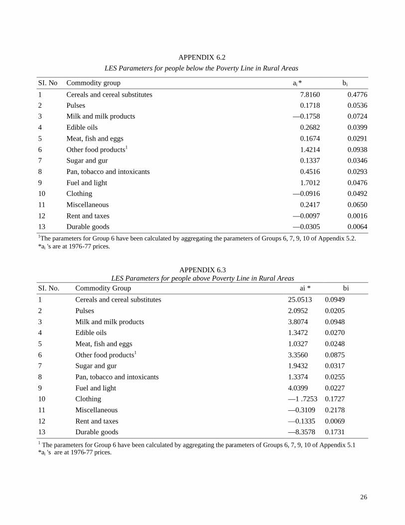
APPENDIX 6.2

LES Parameters for people below the Poverty Line in Rural Areas

SI. No Commodity group ai * bi

1 Cereals and cereal substitutes 7.8160 0.4776

2 Pulses 0.1718 0.0536

3 Milk and milk products —0.1758 0.0724

4 Edible oils 0.2682 0.0399

5 Meat, fish and eggs 0.1674 0.0291

6 Other food products1 1.4214 0.0938

7 Sugar and gur 0.1337 0.0346

8 Pan, tobacco and intoxicants 0.4516 0.0293

9 Fuel and light 1.7012 0.0476

10 Clothing —0.0916 0.0492

11 Miscellaneous 0.2417 0.0650

12 Rent and taxes —0.0097 0.0016

13 Durable goods —0.0305 0.0064 1The parameters for Group 6 have been calculated by aggregating the parameters of Groups 6, 7, 9, 10 of Appendix 5.2. *ai 's are at 1976-77 prices.

APPENDIX 6.3 LES Parameters for people above Poverty Line in Rural Areas

SI. No. Commodity Group ai * bi


2 Pulses 2.0952 0.0205

3 Milk and milk products 3.8074 0.0948

4 Edible oils 1.3472 0.0270



7 Sugar and gur 1.9432 0.0317

8 Pan, tobacco and intoxicants 1.3374 0.0255


10 Clothing —1 .7253 0.1727

11 Miscellaneous —0.3109 0.2178

12 Rent and taxes —0.1335 0.0069

13 Durable goods —8.3578 0.1731 1 The parameters for Group 6 have been calculated by aggregating the parameters of Groups 6, 7, 9, 10 of Appendix 5.1 *ai 's are at 1976-77 prices.

27

APPENDIX 6.4 LES Parameters for Urban Areas

SI. No. Commodity Group ai bi

1. Cereals and cereal substitutes 11.6438 0.0661

2 Pulses 0.8630 0.0173


4 'Edible oils 0.7562 0.0332


6 Other food products1 —1.6982 0.1986

7 Sugar and gur 0.7533 0.0207

8 Pan, tobacco & intoxicants 0.190Q 0.0277


10 Clothing —2.4354 0.0937


12 Rent and taxes —1.2888 0.0660

13 Durable goods —2.2581 0.0587 1The parameters for Group 6 have been calculated by aggregating the parameters of Groups 6, 7, 9, 10 of Appendix 5.1. NOTE : ai 's are at_1976-77 prices.

APPENDIX 6.5 LES Parameters for people below the Poverty Line in Urban Areas



2 Pulses 0.1824 0.0416


4 Edible oils 0.0694 0.0568

5 Meat, fish and eggs —0.0798 0.0404


7 Sugar and gur 0.1303 0.0393

8 Pan, tobacco & intoxicants 0.2758 0.0267


10 Clothing —0.5347 0.0433


12 Rent and taxes —0.3136 0.0391

13 Durable goods —0.1109 0.0077 1 The parameters for Group 6 have been calculated by aggregating the parameters of Groups 6, 7, 9, 10 of Appendix 5.3. NOTE : ai 's are at J 976-77 prices,

28

APPENDIX 6.6

LES Parameters for people above the Poverty Line in Urban Areas



2 Pulses 2.9387 0.0057

3 Milk and milk products 6.7912 0.0860

4 Edible oils 4.1835 0.0153



7 Sugar and gur 3.1248 0.0109

8 Pan, tobacco & intoxicants 0.8975 0.0296


10 Clothing —2.3538 0.1168


12 Rent and taxes —0.18.98 0.0757

13 Durable goods —7.0532 0.1014 xThe parameters for Group 6 have been calculated by aggregating the parameters of Groups 6, 7, 9, 10 of Appendix 5.3. NOTE : a; 's are at 1976-77 prices.

APPENDIX 7.1

Revised LES Parameters and monthly Per Capita Consumption Expenditure (ci) in Rural Area* Corresponding to the balanced Rural Private Consumption*

SI. No. Commodity Group ai bi Ci

1 Cereals and cereal substitutes 10.4752 0.1252 20. ,1987

2 Pulses 0.3272 0.0163 1. ,5966

3 Milk & milk products —1.2802 0.0955 6. ,1358

4 Edible oils 0.2394 0.0271 2, ,3459

5 Meat, fish & eggs 0.0606 0.0369 2. ,9274

6 Other food products 0.7753 0.1218 10 .2307

7 Sugar and gur —0.0272 0.0417 3 .2079

8 Pan, tobacco & intoxicants 0.3456 0.0305 2 .7160

9 Fuel and light 0.6919 0.0093 1 .4131

10 Clothing —3.9247 0.1369 6 .7061

11 Miscellaneous —5.3266 0.2077 10 .8001

12 Rent and taxes —0.5330 0.0160 0 .7060

—6.0040 0.1351 4 .4795 13 Durable goods Total

—4.1805 1.0000 73 .4638

* As given in Appendix 3.

29

APPENDIX 7.2

Revised LES Parameters and monthly Per Capita Consumption Expenditure (C/) for people below the Poverty Line in Rural Areas Corresponding to Balanced Rural Private Consumption*

SI. No. Commodity Group ai bi Ci (Rs.)


2 Pulses 0.1181 0.0335 1.2159

3 Milk & milk products —0.2059 0.0771 2.3221

4 Edible oils 0.3108 0.0421 1.6910

5 Meat, fish & eggs 0.3015 0.0477 1 . 8643


7 Sugar and gur 0.1876 0.0442 1.6359

8 Pan, tobacco & intoxicants 0.6403 0.0378 1.8789

9 Fuel and light 0.6191 0.0158 1.1357

10 Clothing —0.1119 0.0644 1.9985

11 Miscellaneous 0.3803 0.0930 3.4294

12 Rent and taxes —0.0449 0.0068 0.1765

13 Durable goods —0.1264 0.0241 0.6644

Total 11.1093 1.0000 438.849

*As given in Appendix 4.1.

APPENDIX 7.3

Revised LES Parameters and monthly Per Capita Consumption Expenditure (Ci ) for people below the Poverty Line in Urban Areas Corresponding to Balanced Urban Private Consumption*



2 Pulses 1.2025 0.0076 1.9227


4 Edible oils 1.3055 0.0168 2.9069

5 Meat, fish & eggs 1.5539 0.0239 3.8380


7 Sugar and gur 2.2789 0.0239 4.5513


9 Fuel and light 1.2283 0.0044 1.6507

10 Clothing —2.0944 0.1345 10.7381

11 Miscellaneous —0.4087 0.1837 17.1132

12 Rent and taxes —0.4792 0.0172 1.1594

13 Durable goods —28.9378 0.3846 7.7471

Total 3.4153 1.0000 98.7991

* As given in Appendix 44,

30

APPENDIX 7.4

Revised LES Parameters and monthly Per Capita Consumption Expenditure (CO in Urban Areas corresponding to balanced Urban Private Consumption*



2 Pulses 0.4689 0.0084 1.6280

3 Milk & milk products —0.7430 0.0820 7.5292

4 Edible oils 0.6278 0.0247 3.1239

5 Meat, fish & eggs 0.1171 0.0397 4.1216

6 Other food products —2.2548 0.2366 21.6280

7 Sugar and gur 0.8609 0.0212 3.0033


9 Fuel and light 0.5282 0.0100 1.5352

10 Clothing —2.0462 0.0706 5.0840

11 Miscellaneous —4.7645 0.2330 18.7560

12 Rent and taxes —3.3201 0.1526 12.0791

13 Durable good 2.3485 0.0548 3.1808

Total —4.6916 1.0000 96.2375 *As given in Appendix 3.

APPENDIX 7.5

Revised LES Parameters and monthly Per Capita Consumption Expenditure (C/) for people below the Poverty Line in Urban Areas Corresponding to Balanced Urban Private Consumption*

SI. No. Commodity Groups ai bi Ci (Rs.)

1 Cereals and cereal substitutes 4.0325 0.1735 12.2682 2. Pulses 0.0875 0.0211 0.0900 3 Milk and milk products —0.8419 0.0914 3.4953 4 Edible oils 0.0519 0.0450 2.1884 5 Meat, fish & eggs —0.0963 0.0516 2.3555 6 Other food products 1.1076 0.2027 10.7292 7 Sugar and gur 0.1279 0.0408 2.0670 8 Pan, tobacco & intoxicants 0.2882 0.0295 1.6906 9 Fuel and light 0.3021 0.0166 1.0901 10 Clothing —0.4929 0.0423 1.5132 11 Miscellaneous —0.4913 0.1592 7.0676 12 Rent and taxes —0.8390 0.1107 4.4180 13 Durable goods —0.2104 0.0155 0.5235

Total .. 3.0260 1.0000 50.4960

* As given in Appendix 4.2.

31

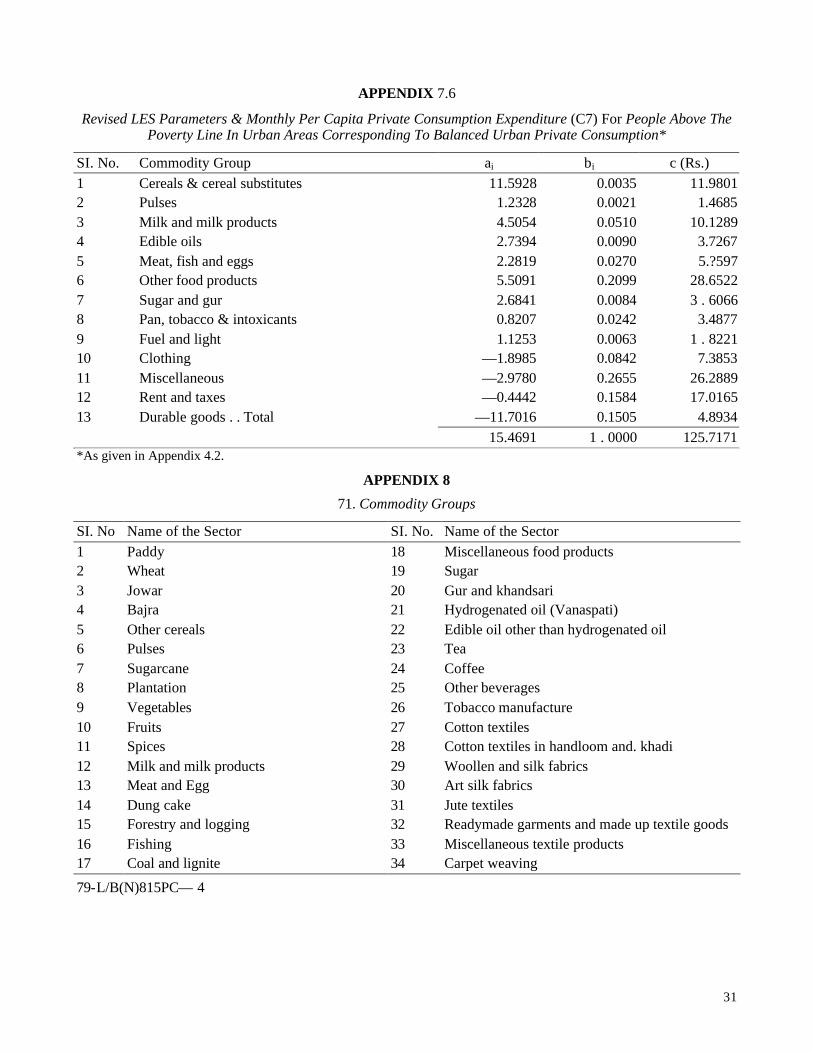
APPENDIX 7.6

Revised LES Parameters & Monthly Per Capita Private Consumption Expenditure (C7) For People Above The Poverty Line In Urban Areas Corresponding To Balanced Urban Private Consumption*

SI. No. Commodity Group ai bi c (Rs.)

1 Cereals & cereal substitutes 11.5928 0.0035 11.9801 2 Pulses 1.2328 0.0021 1.4685 3 Milk and milk products 4.5054 0.0510 10.1289 4 Edible oils 2.7394 0.0090 3.7267 5 Meat, fish and eggs 2.2819 0.0270 5.?597 6 Other food products 5.5091 0.2099 28.6522 7 Sugar and gur 2.6841 0.0084 3 . 6066 8 Pan, tobacco & intoxicants 0.8207 0.0242 3.4877 9 Fuel and light 1.1253 0.0063 1 . 8221 10 Clothing —1.8985 0.0842 7.3853 11 Miscellaneous —2.9780 0.2655 26.2889 12 Rent and taxes —0.4442 0.1584 17.0165

—11.7016 0.1505 4.8934 13 Durable goods . . Total

15.4691 1 . 0000 125.7171 *As given in Appendix 4.2.

APPENDIX 8

71. Commodity Groups

SI. No Name of the Sector SI. No. Name of the Sector

1 Paddy 18 Miscellaneous food products 2 Wheat 19 Sugar 3 Jowar 20 Gur and khandsari 4 Bajra 21 Hydrogenated oil (Vanaspati) 5 Other cereals 22 Edible oil other than hydrogenated oil 6 Pulses 23 Tea 7 Sugarcane 24 Coffee 8 Plantation 25 Other beverages 9 Vegetables 26 Tobacco manufacture 10 Fruits 27 Cotton textiles 11 Spices 28 Cotton textiles in handloom and. khadi 12 Milk and milk products 29 Woollen and silk fabrics 13 Meat and Egg 30 Art silk fabrics 14 Dung cake 31 Jute textiles 15 Forestry and logging 32 Readymade garments and made up textile goods 16 Fishing 33 Miscellaneous textile products 17 Coal and lignite 34 Carpet weaving

79-L/B(N)815PC— 4

32

APPENDIX 8-contd. SI. No. Name of the Sector SI. No. Name of the Sector 35 Wood products 54 Electrical household goods 36 Paper, paper products and newsprint 55 Communication and electronic equipment 37 Printing and publishing 56 Other electrical machinery 38 Leather and leather products 57 Motor vehicles 39 Leather footwear 58 Motor cycles and bicycles 40 Rubber products 59 Watches and clocks 41 Plastics 60 Miscellaneous manufacturing industries 42 Petroleum products 61 Gas, electricity and water supply 43 Miscellaneous coal and petroleum products 62 Railways 44 Insecticides, Fungicides 63 Other transport 45 Soaps and glycerine 64 Communication 46 Cosmetics 65 Banking and insurance 47 Other chemicals 66 Real estate and ownership of dwellings 48 Other non-metallic mineral products 67 Consumer rent 49 Metal products 68 Education 50 Office, domestic and commercial equipment 69 Medicines 51 Other non-electrical machinery 70 Doctor, nurse, midwife 52 Electrical cables and wires 71 Other services 53 Batteries

APPENDIX 9.1 Demand Function Parameters For People Below The Poverty Line in Rural Areas

Parameters at 1973-74 prices Parameters at 1976-77 prices and adjusted for LES Total for 1977-78

Commodity Group

Input-Output Sector No.

LES Group Demand Function No.

ai bi ai bi 1 2 3 4 5 6 7 8 1 1 1 1 — .84866 0.88384 —1.036393 .883840 2 2 1 5 —1.75126 0.14853 —2.138065 .144032 3 3 1 1 —0.94533 0.50049 —1.234284 .500490 4 4 1 2 —2.08960 0.91993 —1.653515 .660927 5 5 1 1 0.96598 0.00682 .444230 .006820 6 6 2 5 —0.54081 0.05448 — .484206 .038739 7 7 7 7 0.00268 0.0 .001992 0.000000 8 10 4 7 —0.00205 0.0 .002326 0.000000 9 11 6 5 —0.04703 0.04713 — .097234 .075048

10 11 6 1 —5.34741 1.20883 —4.901424 1.208830 11 11 6 1 —2.73601 0.78666 —2.192794 0.78666 12 12 3 1 —10.58516 3.06148 —10.917261 3.061480 13 13 5 1 —6.72108 1.55410 —6.250798 1.554100 14 13 5 5 —0.10152 0.01152 — .232397 .020932 15 14 9 1 —1.37235 0.49599 —2.515075 .495990 16 15 5 5 —0.00709 0.01130 — .008244 .010896 17 16 9 1 —8.86927 1.43192 —8.841874 1.431920 18 20 6 5 0.10049 0.00473 .167194 .006242

33

APPENDIX 9.1—contd.

1 2 3 4 5 6 7 8 19 21 7 1 —8.45839 2.07118 —8.724376 2.071180 20 22 7 1 —6.91487 1.79771 -6.741341 1.797710 21 23 4 7 0.0 0.0 0.000000 0.000000 22 24 4 1 —4.48536 1.32746 —4.571686 1.327460 23 25 6 1 —5.96904 1.36895 —5.958862 1.368950 24 25 6 1 —9.97205 1.74000 —10.047332 1.740000 25 26 6 6 0.18109 —1.60915 .447512 —5.006562 26 27 8 1 —3.17692 0.79214 —2.358961 .792140 27 28 10 1 —8.70433 2.27048 —8.653991 2.270480 28 29 10 2 —0.08894 0.05304 —.748304 .392356 29 30 10 7 0.0 0.0 0.000000 0.000000 30 31 10 7 0.0 0.0 0.000000 0.000000 31 32 10 7 0.0 0.0 0.000000 0.000000 32 33 10 2 —0.05917 0.03350 — .277588 .139029 33 34 10 7 0.0 0.0 0.000000 0.000000 34 35 10 7 0.00003 0.0 .000312 0.000000 35 36 13 7 0.0 0.0 0.000000 0.000000 36 37 11 7 0.0 0.0 0.000000 0.000000 37 38 11 7 0.00003 0.0 .000015 0.000000 38 39 13 7 0.0 0.0 0.000000 0.000000 39 40 13 7 0.00074 0.0 .001623 0.000000 40 41 13 7 0.0 0.0 0.000000 0.000000 41 42 11 7 0.0 0.0 0.000000 0.000000 42 43 9 5 0.09934 0.00773 .156193 .009649 43 44 9 7 0.0 0.0 0.000000 0.000000 44 48 11 7 0.0 0.0 0.000000 0.000000 45 50 11 1 —7.08724 1.56813 —7.658326 1.568130 46 51 11 1 —3.77767 0.12616 —5.402824 .726160 47 53 11 1 —7.37336 1.45987 —7.351514 1.459870 48 56 13 7 0.00185 0.0 .002654 0.000000 49 61 13 7 0.00023 0.0 .000559 0.000000 50 64 13 7 0.0 0.0 0.000000 0.000000 51 65 13 7 0.0 0.0 0.000000 0.000000 52 67 13 7 0.0 0.0 0.000000 0.000000 53 68 13 7 0.0 0.0 0.000000 0.000000 54 69 13 7 0.00002 0.0 0.000096 0.000000 55 70 13 7 0.0 0.0 0.000000 0.000000 56 71 13 7 0.0 0.0 0.000000 0.000000 57 74 13 7 0.0 0.0 0.000000 0.000000 58 75 13 7 0.0 0.0 0.000000 0.000000 59 77 11 7 0.0 0.0 0.000000 0.000000

34

APPENDIX 9.1—contd..

1 2 3 4 5 6 7 8 60 78 13 7 0.00397 0.0 0.010206 0.000000 61 80 9 7 0.0000 0.0000 0.000000 0.000000 62 81 11 7 0.0000 0.0000 0.000000 0.000000 63 82 11 1 —7.66071 1.69210 —6.820315 1.692100 64 83 11 7 0.0000 0.0000 0.000000 0.000000 65 85 11 7 0.0000 0.0000 0.000000 0.000000 66 86 12 7 0.00380 0.0 .002010 0.000000 67 86 12 7 0.00380 0.0 .002010 0.000000 68 87 11 7 0.00229 0.0 .007173 0.000000 69 88 11 1 —9.55463 2.31067 —8.923172 2.310670 70 88 11 7 0.0000 0.0000 0.000000 0.000000 71 89 11 1 —5.77799 1.30388 —4.846113 1.303880

N.B.: 1. For key to 71 commodity groups refer to Appendix 8. 2. For key to 89 input-output sectors refer to Appen. 11. 3. For key to 13 LES group numbers refer to Appen. 3. 4. D.F. No. Function/Engel Curves

1 : Double log 2 : Serrii log 5 : Linear 6 : Hyperbola 7 : Proportion (Propensity)

APPENDIX 9.2

Demand Function Parameters For People Above The Poverty Line In Rural Areas.

Parameters at 1973-74 price Parameters at 1976-77 prices and adjusted for LES Totals

for 1977-78 -A

Commodity

Input-Output

Sector No.

LES Group Demand Function

No. ai bi ai bi

1 2 3 4 5 6 7 8 1 1 1 1 0.78234 0.45555 .391045 .455550 2 2 1 1 —1.49159 0.79341 —1.776942 .793410 3 3 1 1 1.43443 —0.17832 .999613 — .178320 4 4 1 1 —0.55964 0.23879 —1.247467 .238790 5 5 1 1 0.09302 0.23810 — .784181 .238100 6 6 2 1 —2.53475 0.82459 —3.125398 . 824590 7 7 7 7 0.00203 0.0 .001627 0.000000 8 10 4 7 0.01191 0.0 .006738 0.000000 9 11 6 1 —2.05758 0.71884 —1.767885 .718840 10 11 6 1 —6.17276 1.45023 —6.051515 1.450230 11 11 6 1 —2.10833 0.61707 —1.795195 .617070 12 12 3 5 —2.52114 0.11986 —3.443398 .130019

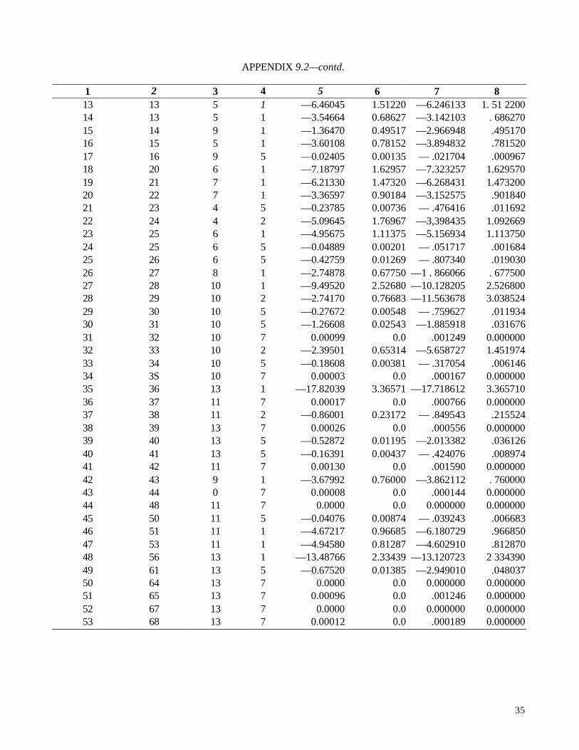
35


1 2 3 4 5 6 7 8 13 13 5 1 —6.46045 1.51220 —6.246133 1. 51 2200 14 13 5 1 —3.54664 0.68627 —3.142103 . 686270 15 14 9 1 —1.36470 0.49517 —2.966948 .495170 16 15 5 1 —3.60108 0.78152 —3.894832 .781520 17 16 9 5 —0.02405 0.00135 — .021704 .000967 18 20 6 1 —7.18797 1.62957 —7.323257 1.629570 19 21 7 1 —6.21330 1.47320 —6.268431 1.473200 20 22 7 1 —3.36597 0.90184 —3.152575 .901840 21 23 4 5 —0.23785 0.00736 — .476416 .011692 22 24 4 2 —5.09645 1.76967 —3,398435 1.092669 23 25 6 1 —4.95675 1.11375 —5.156934 1.113750 24 25 6 5 —0.04889 0.00201 — .051717 .001684 25 26 6 5 —0.42759 0.01269 — .807340 .019030 26 27 8 1 —2.74878 0.67750 —1 . 866066 . 677500 27 28 10 1 —9.49520 2.52680 —10.128205 2.526800 28 29 10 2 —2.74170 0.76683 —11.563678 3.038524 29 30 10 5 —0.27672 0.00548 — .759627 .011934 30 31 10 5 —1.26608 0.02543 —1.885918 .031676 31 32 10 7 0.00099 0.0 .001249 0.000000 32 33 10 2 —2.39501 0.65314 —5.658727 1.451974 33 34 10 5 —0.18608 0.00381 — .317054 .006146 34 3S 10 7 0.00003 0.0 .000167 0.000000 35 36 13 1 —17.82039 3.36571 —17.718612 3.365710 36 37 11 7 0.00017 0.0 .000766 0.000000 37 38 11 2 —0.86001 0.23172 — .849543 .215524 38 39 13 7 0.00026 0.0 .000556 0.000000 39 40 13 5 —0.52872 0.01195 —2.013382 .036126 40 41 13 5 —0.16391 0.00437 — .424076 .008974 41 42 11 7 0.00130 0.0 .001590 0.000000 42 43 9 1 —3.67992 0.76000 —3.862112 . 760000 43 44 0 7 0.00008 0.0 .000144 0.000000 44 48 11 7 0.0000 0.0 0.000000 0.000000 45 50 11 5 —0.04076 0.00874 — .039243 .006683 46 51 11 1 —4.67217 0.96685 —6.180729 .966850 47 53 11 1 —4.94580 0.81287 —4.602910 .812870 48 56 13 1 —13.48766 2.33439 —13.120723 2 334390 49 61 13 5 —0.67520 0.01385 —2.949010 .048037 50 64 13 7 0.0000 0.0 0.000000 0.000000 51 65 13 7 0.00096 0.0 .001246 0.000000 52 67 13 7 0.0000 0.0 0.000000 0.000000 53 68 13 7 0.00012 0.0 .000189 0.000000

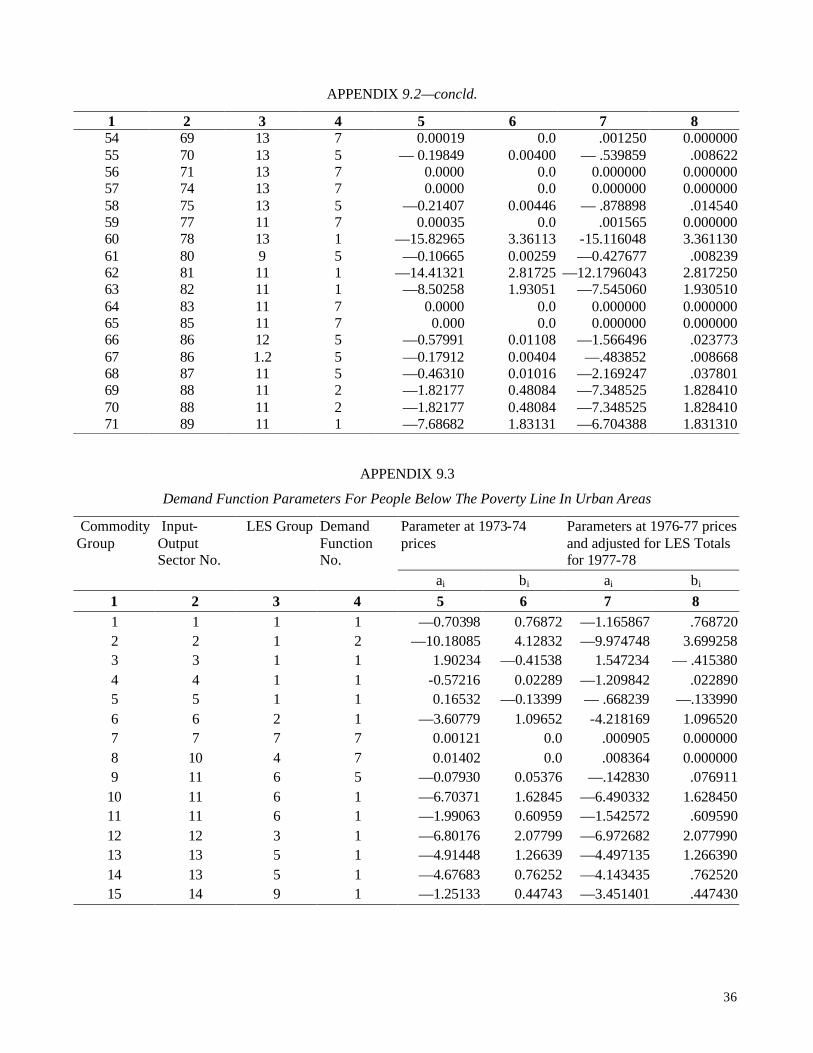
36

APPENDIX 9.2—concld.

1 2 3 4 5 6 7 8 54 69 13 7 0.00019 0.0 .001250 0.000000 55 70 13 5 — 0.19849 0.00400 — .539859 .008622 56 71 13 7 0.0000 0.0 0.000000 0.000000 57 74 13 7 0.0000 0.0 0.000000 0.000000 58 75 13 5 —0.21407 0.00446 — .878898 .014540 59 77 11 7 0.00035 0.0 .001565 0.000000 60 78 13 1 —15.82965 3.36113 -15.116048 3.361130 61 80 9 5 —0.10665 0.00259 —0.427677 .008239 62 81 11 1 —14.41321 2.81725 —12.1796043 2.817250 63 82 11 1 —8.50258 1.93051 —7.545060 1.930510 64 83 11 7 0.0000 0.0 0.000000 0.000000 65 85 11 7 0.000 0.0 0.000000 0.000000 66 86 12 5 —0.57991 0.01108 —1.566496 .023773 67 86 1.2 5 —0.17912 0.00404 —.483852 .008668 68 87 11 5 —0.46310 0.01016 —2.169247 .037801 69 88 11 2 —1.82177 0.48084 —7.348525 1.828410 70 88 11 2 —1.82177 0.48084 —7.348525 1.828410 71 89 11 1 —7.68682 1.83131 —6.704388 1.831310

APPENDIX 9.3

Demand Function Parameters For People Below The Poverty Line In Urban Areas

Parameter at 1973-74 prices

Parameters at 1976-77 prices and adjusted for LES Totals for 1977-78

Commodity Group

Input- Output Sector No.

LES Group Demand Function No.

ai bi ai bi

1 2 3 4 5 6 7 8 1 1 1 1 —0.70398 0.76872 —1.165867 .768720 2 2 1 2 —10.18085 4.12832 —9.974748 3.699258 3 3 1 1 1.90234 —0.41538 1.547234 — .415380 4 4 1 1 -0.57216 0.02289 —1.209842 .022890 5 5 1 1 0.16532 —0.13399 — .668239 —.133990 6 6 2 1 —3.60779 1.09652 -4.218169 1.096520 7 7 7 7 0.00121 0.0 .000905 0.000000 8 10 4 7 0.01402 0.0 .008364 0.000000 9 11 6 5 —0.07930 0.05376 —.142830 .076911

10 11 6 1 —6.70371 1.62845 —6.490332 1.628450 11 11 6 1 —1.99063 0.60959 —1.542572 .609590 12 12 3 1 —6.80176 2.07799 —6.972682 2.077990 13 13 5 1 —4.91448 1.26639 —4.497135 1.266390 14 13 5 1 —4.67683 0.76252 —4.143435 .762520 15 14 9 1 —1.25133 0.44743 —3.451401 .447430

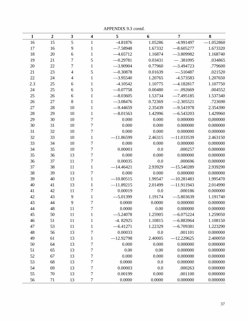
37

APPENDIX 9.3 contd.

1 2 3 4 5 6 7 8 16 15 5 1 -4.81876 1.05286 -4.991497 —1.052860 17 16 9 1 —7.58948 1.67332 —8.605277 1.673320 18 20 6 1 —4.65712 1.16874 —3.809982 1.168740 19 21 7 5 —0.29781 0.03431 — .381095 .034865 20 22 7 1 —3.90904 0.77960 —3.494723 .779600 21 23 4 5 —0.30878 0.01639 —.510487 .021520 22 24 4 1 —3.95540 1.20765 -4.573583 1.207650 2.3 25 6 1 -4.10542 1.10775 —4.182817 1.107750 24 25 6 5 —0.07758 0.00480 — .092669 .004552 25 26 6 1 —8.03605 1.53734 —7.495185 1.537340 26 27 8 1 —3.08476 0.72369 —2.305521 .723690 27 28 10 1 —9.44659 2.35439 —9.541978 2.354390 28 29 10 1 —8.01563 1.42996 —6.543203 1.429960 29 30 10 7 0.000 0.000 0.000000 0,000000 30 31 10 7 0.000 0.000 0.000000 0.000000 31 32 10 7 0.000 0.000 0.000000 0.000000 32 33 10 1 —11.86599 2.46315 —11.033539 2.463150 33 34 10 7 0.000 0.000 0.000000 0.000000 34 35 10 7 0.00003 0.0 .000257 0.000000 35 36 13 7 0.000 0.000 0.000000 0.000000 36 37 11 7 0.00035 0.0 .000696 0.000000 37 38 11 1 —14.46421 2.93929 —15.540289 2.939290 38 39 13 7 0.000 0.000 0.000000 0.000000 39 40 13 1 —10.80515 1.99547 —10.281483 1.995470 40 41 13 I —11.89215 2.01499 —11.911943 2.014990 41 42 11 7 0.00019 0.0 .000186 0.000000 42 43 9 1 —5.01399 1.19174 —5.803639 1.191740 43 44 9 7 0.0000 0.0000 0.000000 0.000000 44 48 11 7 0.0000 0.00 0.000000 0.000000 45 50 11 1 —5.24078 1.25905 —6.075224 1.259050 46 51 11 1 -4. 82925 1.10815 —6.883964 1.108150 47 53 11 1 —6.41271 1.22329 —6.709381 1.223290 48 56 13 7 0.00033 0.0 .001101 0.000000 49 61 13 1 —12.92798 2.40005 —12.229625 2.400050 50 64 13 7 0.000 0.000 0.000000 0.000000 51 65 13 7 0.00 0.00 0.000000 0.000000 52 67 13 7 0.000 0.000 0.000000 0.000000 53 68 13 7 0.0000 0.0 0.000000 0.000000 54 69 13 7 0.00003 0.0 .000263 0.000000 55 70 13 7 0.00199 0.000 .001100 0.000000 56 71 13 7 0.0000 0.0000 0.000000 0.000000

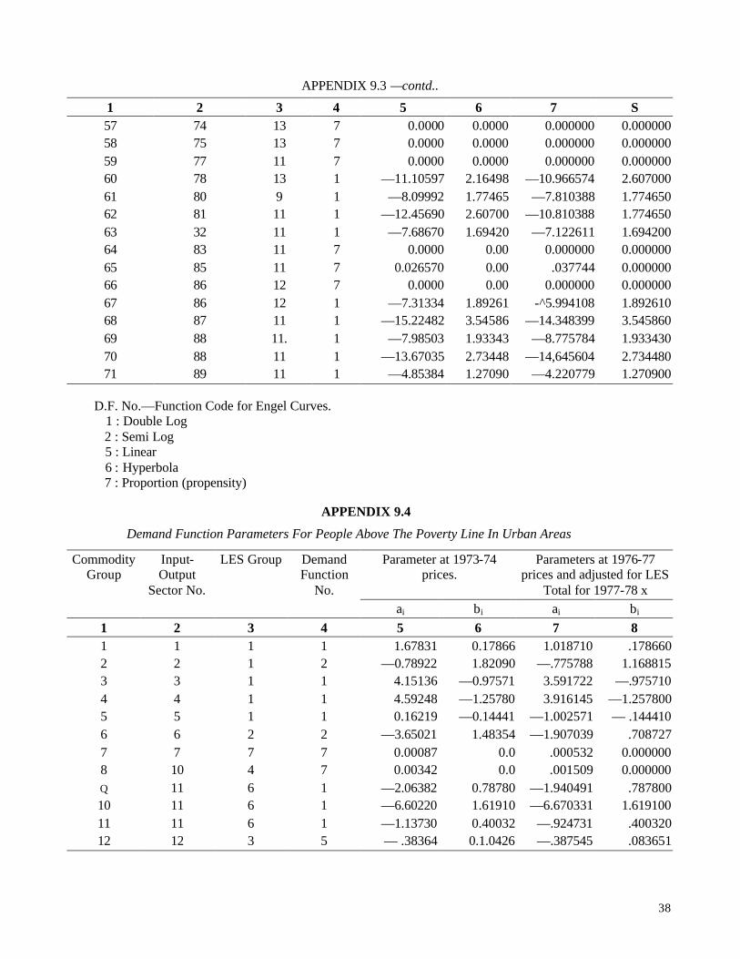
38

APPENDIX 9.3 —contd..

1 2 3 4 5 6 7 S 57 74 13 7 0.0000 0.0000 0.000000 0.000000 58 75 13 7 0.0000 0.0000 0.000000 0.000000 59 77 11 7 0.0000 0.0000 0.000000 0.000000 60 78 13 1 —11.10597 2.16498 —10.966574 2.607000 61 80 9 1 —8.09992 1.77465 —7.810388 1.774650 62 81 11 1 —12.45690 2.60700 —10.810388 1.774650 63 32 11 1 —7.68670 1.69420 —7.122611 1.694200 64 83 11 7 0.0000 0.00 0.000000 0.000000 65 85 11 7 0.026570 0.00 .037744 0.000000 66 86 12 7 0.0000 0.00 0.000000 0.000000 67 86 12 1 —7.31334 1.89261 -^5.994108 1.892610 68 87 11 1 —15.22482 3.54586 —14.348399 3.545860 69 88 11. 1 —7.98503 1.93343 —8.775784 1.933430 70 88 11 1 —13.67035 2.73448 —14,645604 2.734480 71 89 11 1 —4.85384 1.27090 —4.220779 1.270900

D.F. No.—Function Code for Engel Curves. 1 : Double Log 2 : Semi Log 5 : Linear 6 : Hyperbola 7 : Proportion (propensity)

APPENDIX 9.4

Demand Function Parameters For People Above The Poverty Line In Urban Areas

Parameter at 1973-74 prices.

Parameters at 1976-77 prices and adjusted for LES

Total for 1977-78 x

Commodity Group

Input-Output

Sector No.

LES Group Demand Function

No.

ai bi ai bi

1 2 3 4 5 6 7 8 1 1 1 1 1.67831 0.17866 1.018710 .178660 2 2 1 2 —0.78922 1.82090 —.775788 1.168815 3 3 1 1 4.15136 —0.97571 3.591722 —.975710 4 4 1 1 4.59248 —1.25780 3.916145 —1.257800 5 5 1 1 0.16219 —0.14441 —1.002571 — .144410 6 6 2 2 —3.65021 1.48354 —1.907039 .708727 7 7 7 7 0.00087 0.0 .000532 0.000000 8 10 4 7 0.00342 0.0 .001509 0.000000 Q 11 6 1 —2.06382 0.78780 —1.940491 .787800 10 11 6 1 —6.60220 1.61910 —6.670331 1.619100 11 11 6 1 —1.13730 0.40032 —.924731 .400320 12 12 3 5 — .38364 0.1.0426 —.387545 .083651

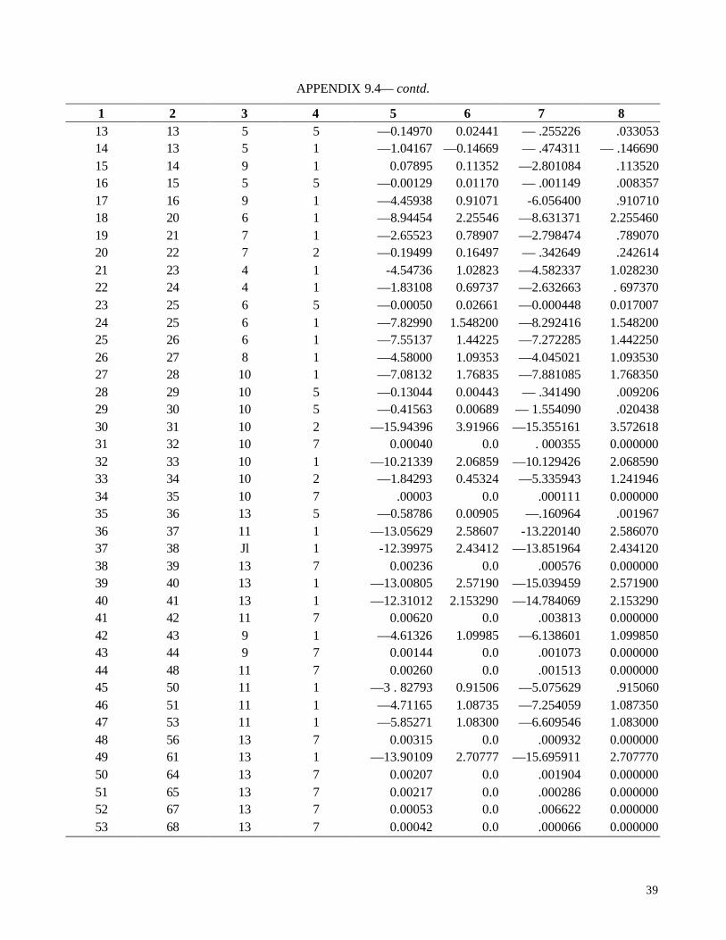
39

APPENDIX 9.4— contd.

1 2 3 4 5 6 7 8 13 13 5 5 —0.14970 0.02441 — .255226 .033053 14 13 5 1 —1.04167 —0.14669 — .474311 — .146690 15 14 9 1 0.07895 0.11352 —2.801084 .113520 16 15 5 5 —0.00129 0.01170 — .001149 .008357 17 16 9 1 —4.45938 0.91071 -6.056400 .910710 18 20 6 1 —8.94454 2.25546 —8.631371 2.255460 19 21 7 1 —2.65523 0.78907 —2.798474 .789070 20 22 7 2 —0.19499 0.16497 — .342649 .242614 21 23 4 1 -4.54736 1.02823 —4.582337 1.028230 22 24 4 1 —1.83108 0.69737 —2.632663 . 697370 23 25 6 5 —0.00050 0.02661 —0.000448 0.017007 24 25 6 1 —7.82990 1.548200 —8.292416 1.548200 25 26 6 1 —7.55137 1.44225 —7.272285 1.442250 26 27 8 1 —4.58000 1.09353 —4.045021 1.093530 27 28 10 1 —7.08132 1.76835 —7.881085 1.768350 28 29 10 5 —0.13044 0.00443 — .341490 .009206 29 30 10 5 —0.41563 0.00689 — 1.554090 .020438 30 31 10 2 —15.94396 3.91966 —15.355161 3.572618 31 32 10 7 0.00040 0.0 . 000355 0.000000 32 33 10 1 —10.21339 2.06859 —10.129426 2.068590 33 34 10 2 —1.84293 0.45324 —5.335943 1.241946 34 35 10 7 .00003 0.0 .000111 0.000000 35 36 13 5 —0.58786 0.00905 —.160964 .001967 36 37 11 1 —13.05629 2.58607 -13.220140 2.586070 37 38 Jl 1 -12.39975 2.43412 —13.851964 2.434120 38 39 13 7 0.00236 0.0 .000576 0.000000 39 40 13 1 —13.00805 2.57190 —15.039459 2.571900 40 41 13 1 —12.31012 2.153290 —14.784069 2.153290 41 42 11 7 0.00620 0.0 .003813 0.000000 42 43 9 1 —4.61326 1.09985 —6.138601 1.099850 43 44 9 7 0.00144 0.0 .001073 0.000000 44 48 11 7 0.00260 0.0 .001513 0.000000 45 50 11 1 —3 . 82793 0.91506 —5.075629 .915060 46 51 11 1 —4.71165 1.08735 —7.254059 1.087350 47 53 11 1 —5.85271 1.08300 —6.609546 1.083000 48 56 13 7 0.00315 0.0 .000932 0.000000 49 61 13 1 —13.90109 2.70777 —15.695911 2.707770 50 64 13 7 0.00207 0.0 .001904 0.000000 51 65 13 7 0.00217 0.0 .000286 0.000000 52 67 13 7 0.00053 0.0 .006622 0.000000 53 68 13 7 0.00042 0.0 .000066 0.000000

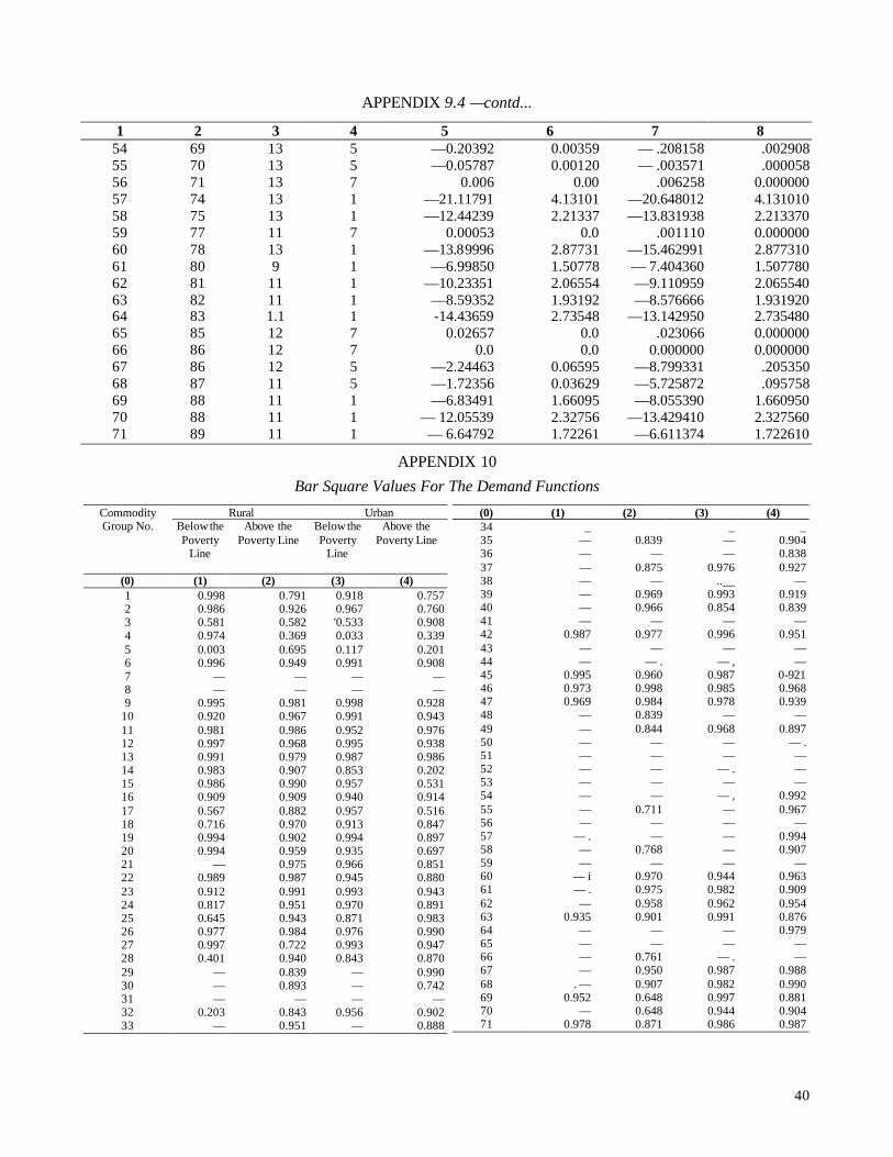
40

APPENDIX 9.4 —contd...

1 2 3 4 5 6 7 8 54 69 13 5 —0.20392 0.00359 — .208158 .002908 55 70 13 5 —0.05787 0.00120 — .003571 .000058 56 71 13 7 0.006 0.00 .006258 0.000000 57 74 13 1 —21.11791 4.13101 —20.648012 4.131010 58 75 13 1 —12.44239 2.21337 —13.831938 2.213370 59 77 11 7 0.00053 0.0 .001110 0.000000 60 78 13 1 —13.89996 2.87731 —15.462991 2.877310 61 80 9 1 —6.99850 1.50778 — 7.404360 1.507780 62 81 11 1 —10.23351 2.06554 —9.110959 2.065540 63 82 11 1 —8.59352 1.93192 —8.576666 1.931920 64 83 1.1 1 -14.43659 2.73548 —13.142950 2.735480 65 85 12 7 0.02657 0.0 .023066 0.000000 66 86 12 7 0.0 0.0 0.000000 0.000000 67 86 12 5 —2.24463 0.06595 —8.799331 .205350 68 87 11 5 —1.72356 0.03629 —5.725872 .095758 69 88 11 1 —6.83491 1.66095 —8.055390 1.660950 70 88 11 1 — 12.05539 2.32756 —13.429410 2.327560 71 89 11 1 — 6.64792 1.72261 —6.611374 1.722610

APPENDIX 10

Bar Square Values For The Demand Functions

Rural Urban Commodity Group No. Below the

Poverty Line

Above the Poverty Line

Below the Poverty

Line

Above the Poverty Line

(0) (1) (2) (3) (4) 1 0.998 0.791 0.918 0.757 2 0.986 0.926 0.967 0.760 3 0.581 0.582 '0.533 0.908 4 0.974 0.369 0.033 0.339 5 0.003 0.695 0.117 0.201 6 0.996 0.949 0.991 0.908 7 — — — — 8 — — — — 9 0.995 0.981 0.998 0.928

10 0.920 0.967 0.991 0.943 11 0.981 0.986 0.952 0.976 12 0.997 0.968 0.995 0.938 13 0.991 0.979 0.987 0.986 14 0.983 0.907 0.853 0.202 15 0.986 0.990 0.957 0.531 16 0.909 0.909 0.940 0.914 17 0.567 0.882 0.957 0.516 18 0.716 0.970 0.913 0.847 19 0.994 0.902 0.994 0.897 20 0.994 0.959 0.935 0.697 21 — 0.975 0.966 0.851 22 0.989 0.987 0.945 0.880 23 0.912 0.991 0.993 0.943 24 0.817 0.951 0.970 0.891 25 0.645 0.943 0.871 0.983 26 0.977 0.984 0.976 0.990 27 0.997 0.722 0.993 0.947 28 0.401 0.940 0.843 0.870 29 — 0.839 — 0.990 30 — 0.893 — 0.742 31 — — — — 32 0.203 0.843 0.956 0.902 33 — 0.951 — 0.888

(0) (1) (2) (3) (4) 34 _ _ _ 35 — 0.839 — 0.904 36 — — — 0.838 37 — 0.875 0.976 0.927 38 — — ..__ — 39 — 0.969 0.993 0.919 40 — 0.966 0.854 0.839 41 — — — — 42 0.987 0.977 0.996 0.951 43 — — — — 44 — — . — , — 45 0.995 0.960 0.987 0-921 46 0.973 0.998 0.985 0.968 47 0.969 0.984 0.978 0.939 48 — 0.839 — — 49 — 0.844 0.968 0.897 50 — — — — . 51 — — — — 52 — — — . — 53 — — — — 54 — — — , 0.992 55 — 0.711 — 0.967 56 — — — — 57 — . — — 0.994 58 — 0.768 — 0.907 59 — — — — 60 — i 0.970 0.944 0.963 61 — . 0.975 0.982 0.909 62 — 0.958 0.962 0.954 63 0.935 0.901 0.991 0.876 64 — — — 0.979 65 — — — — 66 — 0.761 — . — 67 — 0.950 0.987 0.988 68 . — 0.907 0.982 0.990 69 0.952 0.648 0.997 0.881 70 — 0.648 0.944 0.904 71 0.978 0.871 0.986 0.987

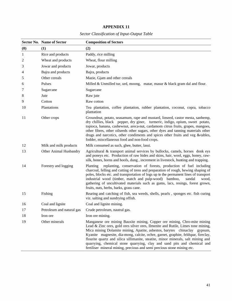
41

APPENDIX 11

Sector Classification of Input-Output Table

Sector No. Name of Sector Composition of Sectors

(0) (1) (2)

1 Rice and products Paddy, rice milling

2 Wheat and products Wheat, flour milling

3 Jowar and products Jowar, products

4 Bajra and products Bajra, products

5 Other cereals Mazie, Gjam and other cereals

6 Pulses Milled & Unmilled tur, urd, moong, matar, masur & black gram dal and flour.

7 Sugarcane Sugarcane

8 Jute Raw jute

9 Cotton Raw cotton

10 Plantations Tea plantation, coffee plantation, rubber plantation, coconut, copra, tobacco plantation

11 Other crops Groundnut, potato, seasamum, rape and mustard, linseed, castor mesta, sanhemp, dry chillies, black pepper, dry giner, turmeric, indigo, opium, sweet potato, topioca, banana, cashewnut, areca-nut, cardamom citrus fruits, grapes, mangoes, other fibres, other oilseeds other sugars, other dyes and tanning materials other drugs and narcotics, other condiments and spices other fruits and veg &-tables, fodder, miscellaneous food and non-food crops.

12 Milk and milk products Milk consumed as such, ghee, butter, lassi.

13 Other Animal Husbandry Agricultural & transport animal services by bullocks, camels, horses donk eys and poneys etc. Production of raw hides and skins, hair, wool, eggs, honey, raw-silk, bones, horns and hoofs, dung , increment in livestock, hunting and trapping.

14 Forestry and logging Planting replanting, conservation of forests, production of fuel including charcoal, felling and cutting of tress and preparation of rough, hewing shaping of poles, blocks etc. and transportation of logs up to the permanent lines of transport industrial wood (timber, match and pulp-wood) bamboo, sandal wood, gathering of uncultivated materials such as gums, lacs, resings, forest grown, fruits, nuts, herbs, barks, grass cane.

15 Fishing Rearing and catching of fish, sea weeds, shells, pearls , sponges etc. fish curing viz. salting and sundrying offish.

16 Coal and lignite Coal and lignite mining.

17 Petroleum and natural gas Crude petroleum, nautral gas.

18 Iron ore Iron ore mining.

19 Other minerals Manganese ore mining Bauxite mining, Copper ore mining, Chro-mite mining Lead & Zinc ores, gold ores silver ores, Ilmenite and Rutile, Limes tone mining, Mica mining Dolamite mining, Apatite, asbestos, barytes chinaclay gypsum, Kyanite magnesite, dia-mong, calcite, ochre, garnet, graphite, feldspar, fireclay, flourite quartz and silica sillimanite, steatite, minor minerals, salt mining and quarrying, chemical stone quarrying, clay and sand pits and chemical and fertiliser mineral mining, precious and semi precious stone mining etc.

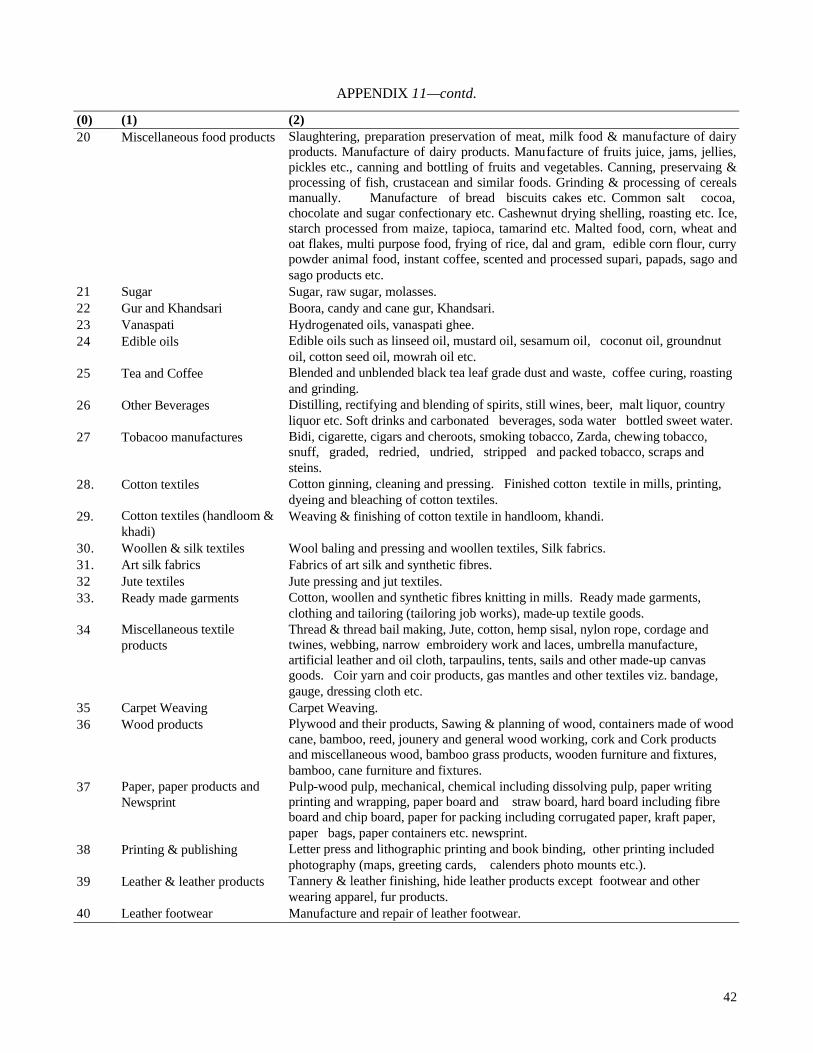
42

APPENDIX 11—contd.

(0) (1) (2) 20 Miscellaneous food products Slaughtering, preparation preservation of meat, milk food & manufacture of dairy

products. Manufacture of dairy products. Manufacture of fruits juice, jams, jellies, pickles etc., canning and bottling of fruits and vegetables. Canning, preservaing & processing of fish, crustacean and similar foods. Grinding & processing of cereals manually. Manufacture of bread biscuits cakes etc. Common salt cocoa, chocolate and sugar confectionary etc. Cashewnut drying shelling, roasting etc. Ice, starch processed from maize, tapioca, tamarind etc. Malted food, corn, wheat and oat flakes, multi purpose food, frying of rice, dal and gram, edible corn flour, curry powder animal food, instant coffee, scented and processed supari, papads, sago and sago products etc.

21 Sugar Sugar, raw sugar, molasses. 22 Gur and Khandsari Boora, candy and cane gur, Khandsari. 23 Vanaspati Hydrogenated oils, vanaspati ghee. 24 Edible oils Edible oils such as linseed oil, mustard oil, sesamum oil, coconut oil, groundnut

oil, cotton seed oil, mowrah oil etc. 25 Tea and Coffee Blended and unblended black tea leaf grade dust and waste, coffee curing, roasting

and grinding. 26 Other Beverages Distilling, rectifying and blending of spirits, still wines, beer, malt liquor, country

liquor etc. Soft drinks and carbonated beverages, soda water bottled sweet water. 27 Tobacoo manufactures Bidi, cigarette, cigars and cheroots, smoking tobacco, Zarda, chewing tobacco,

snuff, graded, redried, undried, stripped and packed tobacco, scraps and steins.

28. Cotton textiles Cotton ginning, cleaning and pressing. Finished cotton textile in mills, printing, dyeing and bleaching of cotton textiles.

29. Cotton textiles (handloom & khadi)

Weaving & finishing of cotton textile in handloom, khandi.

30. Woollen & silk textiles Wool baling and pressing and woollen textiles, Silk fabrics. 31. Art silk fabrics Fabrics of art silk and synthetic fibres. 32 Jute textiles Jute pressing and jut textiles. 33. Ready made garments Cotton, woollen and synthetic fibres knitting in mills. Ready made garments,

clothing and tailoring (tailoring job works), made-up textile goods. 34 Miscellaneous textile

products Thread & thread bail making, Jute, cotton, hemp sisal, nylon rope, cordage and twines, webbing, narrow embroidery work and laces, umbrella manufacture, artificial leather and oil cloth, tarpaulins, tents, sails and other made-up canvas goods. Coir yarn and coir products, gas mantles and other textiles viz. bandage, gauge, dressing cloth etc.

35 Carpet Weaving Carpet Weaving. 36 Wood products Plywood and their products, Sawing & planning of wood, containers made of wood

cane, bamboo, reed, jounery and general wood working, cork and Cork products and miscellaneous wood, bamboo grass products, wooden furniture and fixtures, bamboo, cane furniture and fixtures.

37 Paper, paper products and Newsprint

Pulp-wood pulp, mechanical, chemical including dissolving pulp, paper writing printing and wrapping, paper board and straw board, hard board including fibre board and chip board, paper for packing including corrugated paper, kraft paper, paper bags, paper containers etc. newsprint.

38 Printing & publishing Letter press and lithographic printing and book binding, other printing included photography (maps, greeting cards, calenders photo mounts etc.).

39 Leather & leather products Tannery & leather finishing, hide leather products except footwear and other wearing apparel, fur products.

40 Leather footwear Manufacture and repair of leather footwear.

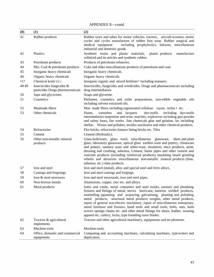
43

APPENDIX ll—contd.

(0) (1) (2) 41 Rubber products Rubber tyres and tubes for motor vehicles, tractors, aircraft-scooters, motor

cycles and cycles manufacture of rubber foot wear. Rubber surgical and medical equipment including prophylactics, baloons, miscellaneous industrial and domestic goods.

42 Plastics Synthetic resins and plastic materials, plastic products manufacture celluloid and its articles and synthetic rubber.

43 Petroleum products Products of petroleum refineries. 44 Mis. Coal & petroleum products Coke and other miscellaneous products of petroleum and coal. 45 Inorganic heavy chemicals Inorganic heavy chemicals.

46 Organic heavy chemicals Organic heavy chemicals. •17 Chemical kruti/.t:r-; Inorganic organic and. mixed fertilizer^ including manures. 48 49 Insecticides fungicides &

pesticides Drugs pharmaceuticais Insecticides, fungicides and weedicides. Drugs and pharmaceuticais including drug intermediaries.

50 Saps and glycerines Soaps and glycerine. 51 Cosmetics Perfumes, cosmetics and toilet preparations, non-edible vegetable oils

including solvent extracted oils. 52 Manmade fibres Man made fibres including regenerated cellulose rayon, nylon • etc. 53 Other chemicals Paints, varnishes and lacquers dye-stuffs including dye-stuffs

intermediaries turpentine and resin, matches, explosives including gun powder and safety fuses, fire works fine chemicals glue and gelatine, lac including shellac. Waxes and polishes, textiles auxiliaries and other chemical products.

54 Refractories Fire bricks, refractories furnace lining bricks etc. Tiles 55 Cement Cement (Hydraulic). 56 Other non-metallic mineral

products Glass-holloware, glass wool, miscellaneous glassware, sheet and plate glass, laboratory glassware, optical glass earthen ware and pottery, chinaware and pottery, sanitary ware and white-ware, insulators, mica products, stone dressing and crushing, asbestos, Cement, hume pipes and other cement and concrete products (including reinforced products) insulating board grinding wheels and abrasives miscellaneous non-metallic mineral products (lime, asbestos, etc.) slate products.

57 Iron and steel Iron and steel (metal), alloy and special steel and ferro alloys. 58 Castings and forgoings Iron and steel castings and forgings.

59 Iron & steel structures Iron and steel structurals, iron and steel pipes. 60 Non-ferrous metals Aluminium, copper, zinc etc. and alloys. 61 Meial products Safes and vaults, metal containers and steel trunks, sanitary and plumbing

fixtures and fittings of metal, stoves hurricane, lanterns welded products, enamelling japanning and acquering, galvanising, planting and polishing metal products, structural metal products weights, other metal products, repair of general non-electric machinery, repair of miscellaneous enterprises, metal furniture and fixtures, hand tools and small tools, bolts, nuts, hails screws springs chains etc. and other metal fittings for shoes, leather, wearing apparel etc. cutlery, locks, type founding razor blades.

62 Tractors & agricultural implements

Tractors and other agricultural machinery, equipments and im plements.

63 Machine tools Machine tools. 64 Office, domestic and commercial

equipments Computing and accounting machines, calculating machines, typewriters and duplicators.

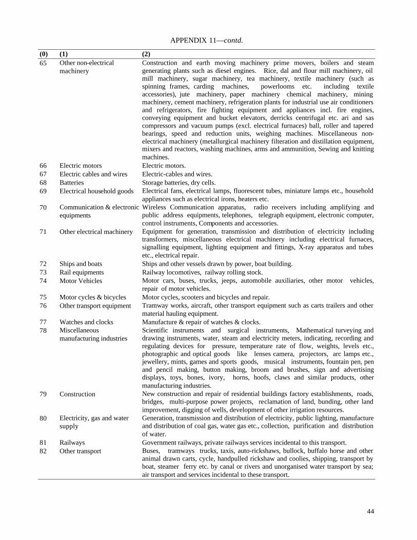
44

APPENDIX 11—contd.

(0) (1) (2) 65 Other non-electrical

machinery Construction and earth moving machinery prime movers, boilers and steam generating plants such as diesel engines. Rice, dal and flour mill machinery, oil mill machinery, sugar machinery, tea machinery, textile machinery (such as spinning frames, carding machines, powerlooms etc. including textile accessories), jute machinery, paper machinery chemical machinery, mining machinery, cement machinery, refrigeration plants for industrial use air conditioners and refrigerators, fire fighting equipment and appliances incl. fire engines, conveying equipment and bucket elevators, derricks centrifugal etc. ari and sas compressors and vacuum pumps (excl. electrical furnaces) ball, roller and tapered bearings, speed and reduction units, weighing machines. Miscellaneous non-electrical machinery (metallurgical machinery filteration and distillation equipment, mixers and reactors, washing machines, arms and ammunition, Sewing and knitting machines.

66 Electric motors Electric motors. 67 Electric cables and wires Electric-cables and wires. 68 Batteries Storage batteries, dry cells. 69 Electrical household goods Electrical fans, electrical lamps, fluorescent tubes, miniature lamps etc., household

appliances such as electrical irons, heaters etc. 70 Communication & electronic

equipments Wireless Communication apparatus, radio receivers including amplifying and public address equipments, telephones, telegraph equipment, electronic computer, control instruments, Components and accessories.

71 Other electrical machinery Equipment for generation, transmission and distribution of electricity including transformers, miscellaneous electrical machinery including electrical furnaces, signalling equipment, lighting equipment and fittings, X-ray apparatus and tubes etc., electrical repair.

72 Ships and boats Ships and other vessels drawn by power, boat building. 73 Rail equipments Railway locomotives, railway rolling stock. 74 Motor Vehicles Motor cars, buses, trucks, jeeps, automobile auxiliaries, other motor vehicles,

repair of motor vehicles. 75 Motor cycles & bicycles Motor cycles, scooters and bicycles and repair. 76 Other transport equipment Tramway works, aircraft, other transport equipment such as carts trailers and other

material hauling equipment. 77 Watches and clocks Manufacture & repair of watches & clocks. 78 Miscellaneous

manufacturing industries Scientific instruments and surgical instruments, Mathematical turveying and drawing instruments, water, steam and electricity meters, indicating, recording and regulating devices for pressure, temperature rate of flow, weights, levels etc., photographic and optical goods like lenses camera, projectors, arc lamps etc., jewellery, mints, games and sports goods, musical instruments, fountain pen, pen and pencil making, button making, broom and brushes, sign and advertising displays, toys, bones, ivory, horns, hoofs, claws and similar products, other manufacturing industries.

79 Construction New construction and repair of residential buildings factory establishments, roads, bridges, multi-purpose power projects, reclamation of land, bunding, other land improvement, digging of wells, development of other irrigation resources.

80 Electricity, gas and water supply

Generation, transmission and distribution of electricity, public lighting, manufacture and distribution of coal gas, water gas etc., collection, purification and distribution of water.

81 Railways Government railways, private railways services incidental to this transport. 82 Other transport Buses, tramways trucks, taxis, auto-rickshaws, bullock, buffalo horse and other

animal drawn carts, cycle, handpulled rickshaw and coolies, shipping, transport by boat, steamer ferry etc. by canal or rivers and unorganised water transport by sea; air transport and services incidental to these transport.

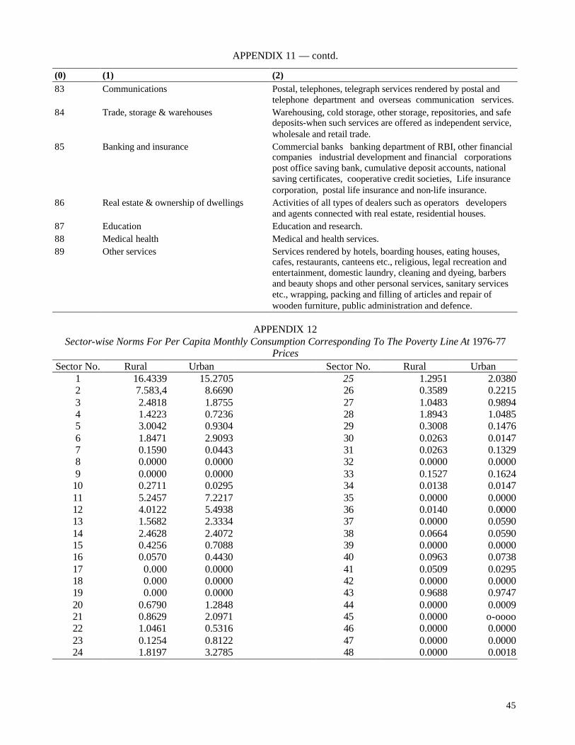
45

APPENDIX 11 — contd.

(0) (1) (2) 83 Communications Postal, telephones, telegraph services rendered by postal and

telephone department and overseas communication services. 84 Trade, storage & warehouses Warehousing, cold storage, other storage, repositories, and safe

deposits-when such services are offered as independent service, wholesale and retail trade.

85 Banking and insurance Commercial banks banking department of RBI, other financial companies industrial development and financial corporations post office saving bank, cumulative deposit accounts, national saving certificates, cooperative credit societies, Life insurance corporation, postal life insurance and non-life insurance.

86 Real estate & ownership of dwellings Activities of all types of dealers such as operators developers and agents connected with real estate, residential houses.

87 Education Education and research. 88 Medical health Medical and health services. 89 Other services Services rendered by hotels, boarding houses, eating houses,

cafes, restaurants, canteens etc., religious, legal recreation and entertainment, domestic laundry, cleaning and dyeing, barbers and beauty shops and other personal services, sanitary services etc., wrapping, packing and filling of articles and repair of wooden furniture, public administration and defence.

APPENDIX 12 Sector-wise Norms For Per Capita Monthly Consumption Corresponding To The Poverty Line At 1976-77

Prices Sector No. Rural Urban Sector No. Rural Urban

1 16.4339 15.2705 25 1.2951 2.0380 2 7.583,4 8.6690 26 0.3589 0.2215 3 2.4818 1.8755 27 1.0483 0.9894 4 1.4223 0.7236 28 1.8943 1.0485 5 3.0042 0.9304 29 0.3008 0.1476 6 1.8471 2.9093 30 0.0263 0.0147 7 0.1590 0.0443 31 0.0263 0.1329 8 0.0000 0.0000 32 0.0000 0.0000 9 0.0000 0.0000 33 0.1527 0.1624

10 0.2711 0.0295 34 0.0138 0.0147 11 5.2457 7.2217 35 0.0000 0.0000 12 4.0122 5.4938 36 0.0140 0.0000 13 1.5682 2.3334 37 0.0000 0.0590 14 2.4628 2.4072 38 0.0664 0.0590 15 0.4256 0.7088 39 0.0000 0.0000 16 0.0570 0.4430 40 0.0963 0.0738 17 0.000 0.0000 41 0.0509 0.0295 18 0.000 0.0000 42 0.0000 0.0000 19 0.000 0.0000 43 0.9688 0.9747 20 0.6790 1.2848 44 0.0000 0.0009 21 0.8629 2.0971 45 0.0000 o-oooo 22 1.0461 0.5316 46 0.0000 0.0000 23 0.1254 0.8122 47 0.0000 0.0000 24 1.8197 3.2785 48 0.0000 0.0018

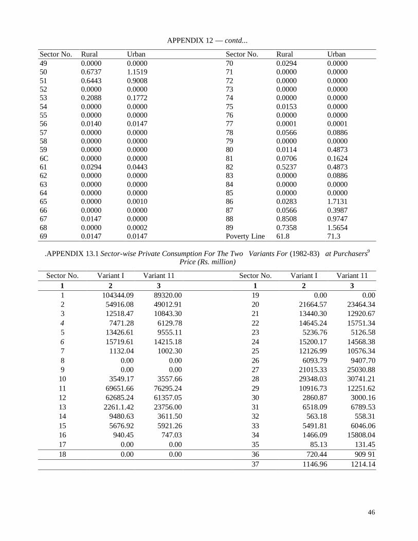
46

APPENDIX 12 — contd...

Sector No. Rural Urban Sector No. Rural Urban 49 0.0000 0.0000 70 0.0294 0.0000 50 0.6737 1.1519 71 0.0000 0.0000 51 0.6443 0.9008 72 0.0000 0.0000 52 0.0000 0.0000 73 0.0000 0.0000 53 0.2088 0.1772 74 0.0000 0.0000 54 0.0000 0.0000 75 0.0153 0.0000 55 0.0000 0.0000 76 0.0000 0.0000 56 0.0140 0.0147 77 0.0001 0.0001 57 0.0000 0.0000 78 0.0566 0.0886 58 0.0000 0.0000 79 0.0000 0.0000 59 0.0000 0.0000 80 0.0114 0.4873 6C 0.0000 0.0000 81 0.0706 0.1624 61 0.0294 0.0443 82 0.5237 0.4873 62 0.0000 0.0000 83 0.0000 0.0886 63 0.0000 0.0000 84 0.0000 0.0000 64 0.0000 0.0000 85 0.0000 0.0000 65 0.0000 0.0010 86 0.0283 1.7131 66 0.0000 0.0000 87 0.0566 0.3987 67 0.0147 0.0000 88 0.8508 0.9747 68 0.0000 0.0002 89 0.7358 1.5654 69 0.0147 0.0147 Poverty Line 61.8 71.3

.APPENDIX 13.1 Sector-wise Private Consumption For The Two Variants For (1982-83) at Purchasers9 Price (Rs. million)

Sector No. Variant I Variant 11 Sector No. Variant I Variant 11 1 2 3 1 2 3 1 104344.09 89320.00 19 0.00 0.00 2 54916.08 49012.91 20 21664.57 23464.34 3 12518.47 10843.30 21 13440.30 12920.67 4 7471.28 6129.78 22 14645.24 15751.34 5 13426.61 9555.11 23 5236.76 5126.58 6 15719.61 14215.18 24 15200.17 14568.38 7 1132.04 1002.30 25 12126.99 10576.34 8 0.00 0.00 26 6093.79 9407.70 9 0.00 0.00 27 21015.33 25030.88

10 3549.17 3557.66 28 29348.03 30741.21 11 69651.66 76295.24 29 10916.73 12251.62 12 62685.24 61357.05 30 2860.87 3000.16 13 2261.1.42 23756.00 31 6518.09 6789.53 14 9480.63 3611.50 32 563.18 558.31 15 5676.92 5921.26 33 5491.81 6046.06 16 940.45 747.03 34 1466.09 15808.04 17 0.00 0.00 35 85.13 131.45 18 0.00 0.00 36 720.44 909 91 37 1146.96 1214.14

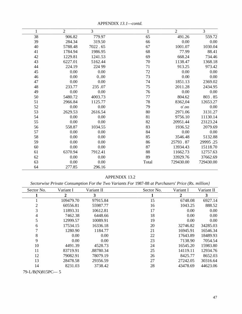
47


1 2 3 1 2 3 38 906.82 779.97 65 491.26 559.72 39 284.34 319.50 66 0.00 0.00 40 5788.48 7022 . 65 67 1001.07 1030.04 41 1784.94 1986.95 68 77.99 88.41 42 1229.81 1241.53 69 668.24 734.46 43 6227.01 5162.44 70 1138.47 1368.18 44 224.19 224 99 71 913.25 973.42 45 0.00 0.00 72 0.00 0.00 46 0.00 0..00 73 0.00 0.00 47 0.00 0.00 74 1851.13 2369.02 48 233.77 235 .07 75 2011.28 2434.95 49 0.00 0.00 76 0.00 0.00 50 5480.72 4003.73 77 804.62 803 . 85 51 2966.84 1125.77 78 8362,04 12653.27 52 0.00 0.00 79 o'.oo 0.00 53 2629.53 2616.54 80 2971.06 3131.27 54 0.00 0.00 81 9756.10 11130.14 55 0.00 0.00 82 20951.44 23123.24 56 558.87 1034.55 83 1936.52 2079.69 57 0.00 0.00 84 0.00 0.00 58 0.00 0.00 85 3546.48 5132.88 59 0.00 0.00 86 25793 . 87 29995 .25 60 0.00 0.00 87 13934.43 15118.70 61 6370.94 7912.41 88 11662.73 12757.63 62 0.00 0.00 89 33929.76 37662.69 63 0.00 0.00 Total 729430.00 729430.00 64 277.85 296.16

APPENDIX 13.2

Sectorwise Private Consumption For the Two Variants For 1987-88 at Purchasers' Price (Rs. million}

Sector No. Variant I Variant II Sector No. Variant I Variant II 1 2 3 1 2 3 1 109479.70 97915.84 15 6748.08 6927.14 2 60556.81 55987.77 16 1043.25 888.52 3 11893.31 10612.81 17 0.00 0.00 4 7462.38 6448.66 18 0.00 0.00 5 12999.57 10089.91 19 0.00 0.00 6 17534.15 16336.18 20 32746.82 34285.03 7 1280.90 1184.77 21 16945.91 16546.34 8 0.00 0.00 22 17643.89 18489.93 9 0.00 0.00 23 7138.90 7054.54 10 4491.39 4528.73 24 16545.20 15983.80 11 83719.91 .88780.34 25 14119.11 12934.76 12 79082.91 78079.19 26 8425.77 8652.03 13 28478.58 29356.59 27 27242.05 30316.64 14 8231.03 3738.42 28 43478.69 44623.06

79-L/B(N)815PC— 5

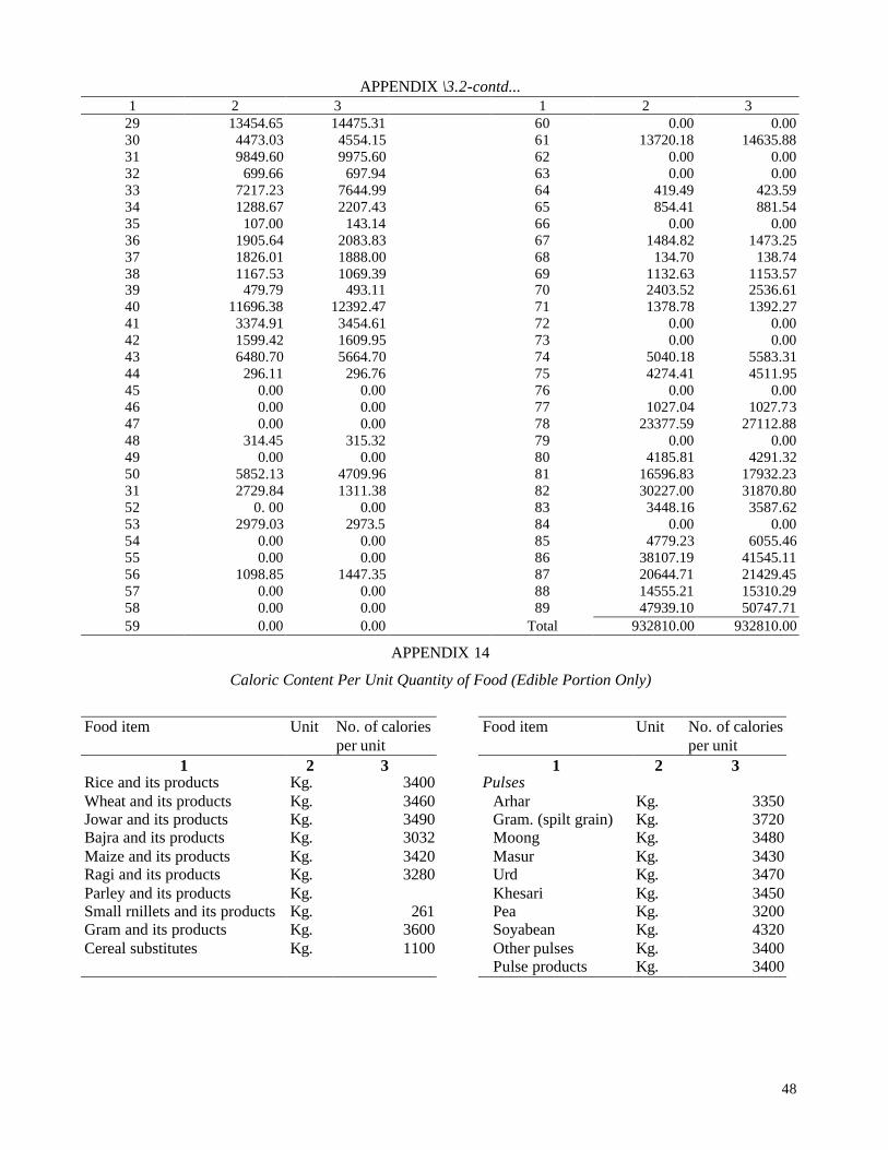
48

APPENDIX \3.2-contd... 1 2 3 1 2 3

29 13454.65 14475.31 60 0.00 0.00 30 4473.03 4554.15 61 13720.18 14635.88 31 9849.60 9975.60 62 0.00 0.00 32 699.66 697.94 63 0.00 0.00 33 7217.23 7644.99 64 419.49 423.59 34 1288.67 2207.43 65 854.41 881.54 35 107.00 143.14 66 0.00 0.00 36 1905.64 2083.83 67 1484.82 1473.25 37 1826.01 1888.00 68 134.70 138.74 38 1167.53 1069.39 69 1132.63 1153.57 39 479.79 493.11 70 2403.52 2536.61 40 11696.38 12392.47 71 1378.78 1392.27 41 3374.91 3454.61 72 0.00 0.00 42 1599.42 1609.95 73 0.00 0.00 43 6480.70 5664.70 74 5040.18 5583.31 44 296.11 296.76 75 4274.41 4511.95 45 0.00 0.00 76 0.00 0.00 46 0.00 0.00 77 1027.04 1027.73 47 0.00 0.00 78 23377.59 27112.88 48 314.45 315.32 79 0.00 0.00 49 0.00 0.00 80 4185.81 4291.32 50 5852.13 4709.96 81 16596.83 17932.23 31 2729.84 1311.38 82 30227.00 31870.80 52 0. 00 0.00 83 3448.16 3587.62 53 2979.03 2973.5 84 0.00 0.00 54 0.00 0.00 85 4779.23 6055.46 55 0.00 0.00 86 38107.19 41545.11 56 1098.85 1447.35 87 20644.71 21429.45 57 0.00 0.00 88 14555.21 15310.29 58 0.00 0.00 89 47939.10 50747.71 59 0.00 0.00 Total 932810.00 932810.00

APPENDIX 14

Caloric Content Per Unit Quantity of Food (Edible Portion Only)

Food item Unit No. of calories

per unit Food item Unit No. of calories

per unit 1 2 3 1 2 3

Rice and its products Kg. 3400 Pulses Wheat and its products Kg. 3460 Arhar Kg. 3350 Jowar and its products Kg. 3490 Gram. (spilt grain) Kg. 3720 Bajra and its products Kg. 3032 Moong Kg. 3480 Maize and its products Kg. 3420 Masur Kg. 3430 Ragi and its products Kg. 3280 Urd Kg. 3470 Parley and its products Kg. Khesari Kg. 3450 Small rnillets and its products Kg. 261 Pea Kg. 3200 Gram and its products Kg. 3600 Soyabean Kg. 4320 Cereal substitutes Kg. 1100 Other pulses Kg. 3400 Pulse products Kg. 3400

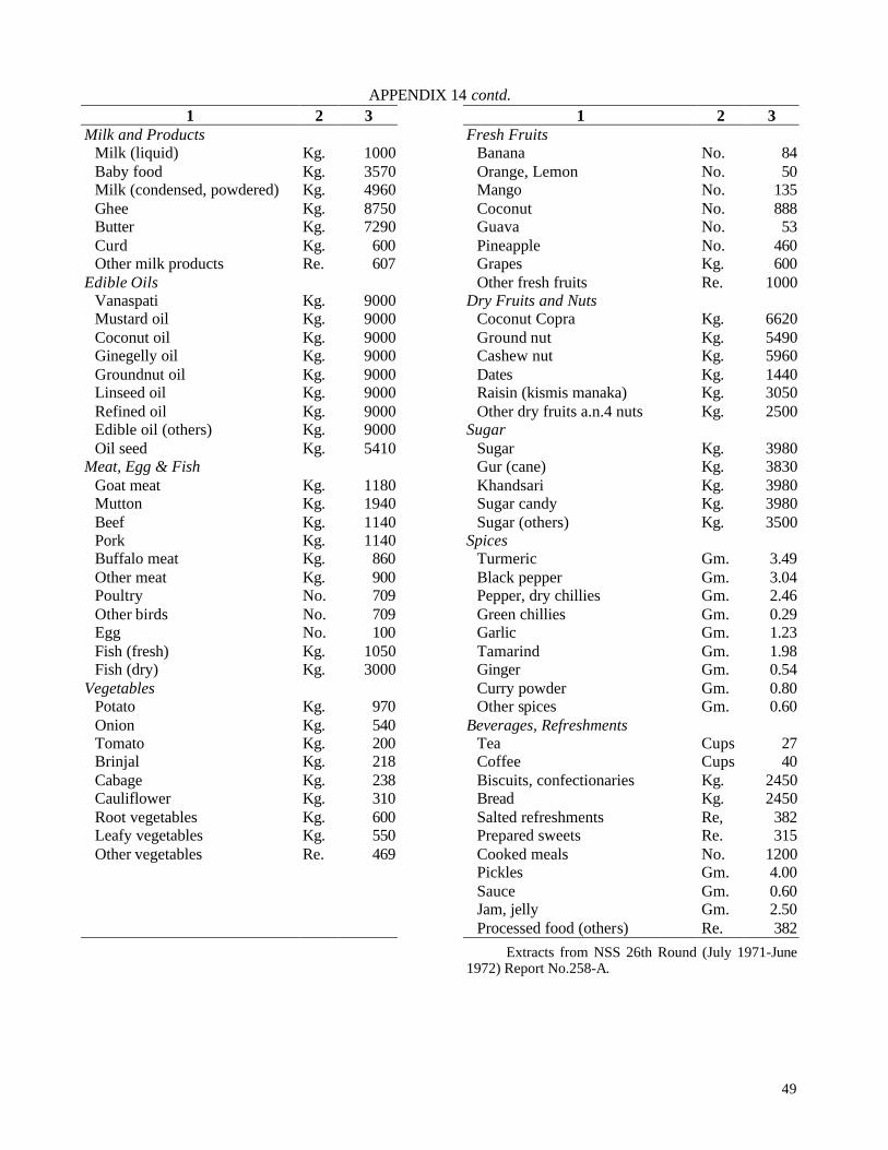
49

APPENDIX 14 contd. 1 2 3 1 2 3

Milk and Products Fresh Fruits Milk (liquid) Kg. 1000 Banana No. 84 Baby food Kg. 3570 Orange, Lemon No. 50 Milk (condensed, powdered) Kg. 4960 Mango No. 135 Ghee Kg. 8750 Coconut No. 888 Butter Kg. 7290 Guava No. 53 Curd Kg. 600 Pineapple No. 460 Other milk products Re. 607 Grapes Kg. 600

Edible Oils Other fresh fruits Re. 1000 Vanaspati Kg. 9000 Dry Fruits and Nuts Mustard oil Kg. 9000 Coconut Copra Kg. 6620 Coconut oil Kg. 9000 Ground nut Kg. 5490 Ginegelly oil Kg. 9000 Cashew nut Kg. 5960 Groundnut oil Kg. 9000 Dates Kg. 1440 Linseed oil Kg. 9000 Raisin (kismis manaka) Kg. 3050 Refined oil Kg. 9000 Other dry fruits a.n.4 nuts Kg. 2500 Edible oil (others) Kg. 9000 Sugar Oil seed Kg. 5410 Sugar Kg. 3980

Meat, Egg & Fish Gur (cane) Kg. 3830 Goat meat Kg. 1180 Khandsari Kg. 3980 Mutton Kg. 1940 Sugar candy Kg. 3980 Beef Kg. 1140 Sugar (others) Kg. 3500 Pork Kg. 1140 Spices Buffalo meat Kg. 860 Turmeric Gm. 3.49 Other meat Kg. 900 Black pepper Gm. 3.04 Poultry No. 709 Pepper, dry chillies Gm. 2.46 Other birds No. 709 Green chillies Gm. 0.29 Egg No. 100 Garlic Gm. 1.23 Fish (fresh) Kg. 1050 Tamarind Gm. 1.98 Fish (dry) Kg. 3000 Ginger Gm. 0.54

Vegetables Curry powder Gm. 0.80 Potato Kg. 970 Other spices Gm. 0.60 Onion Kg. 540 Beverages, Refreshments Tomato Kg. 200 Tea Cups 27 Brinjal Kg. 218 Coffee Cups 40 Cabage Kg. 238 Biscuits, confectionaries Kg. 2450 Cauliflower Kg. 310 Bread Kg. 2450 Root vegetables Kg. 600 Salted refreshments Re, 382 Leafy vegetables Kg. 550 Prepared sweets Re. 315 Other vegetables Re. 469 Cooked meals No. 1200

Pickles Gm. 4.00 Sauce Gm. 0.60 Jam, jelly Gm. 2.50 Processed food (others) Re. 382 Extracts from NSS 26th Round (July 1971-June

1972) Report No.258-A.

50

APPENDIX 15.1 Norms Under The Minimum Needs Programmes As Adopted Earlier And In The Current Exercise

Programme/Project Earlier norms (by end of Fifth Plan) Current norms (by end of the coming

decade of Planning)

1 2 3

Elementary Education To cover 97% of children in age group 6-11 and 47% in the age group 11-14.

100% coverage for all children in the age group 6-14.

Adult Education — Coverage of all those in age group 15-35. Health Establishment of one PHC per each com-

munity development block. Establish-ment of one sub-centre for every 10,000 population. Provision of drugs @ Rs. 12000 per annum for each PHC and Rs. 2000 per annum for each sub-centre.

One PHC for every 35000 population. One sub-centre for every 5000 population. Drugs @ Rs. 50,000 per annum for each PHC, and Rs. 7000 per annum for each sub-centre.

Rural water supply Coverage of all the problem villages. Coverage of all left over problem villages within next five years,

Rural Roads Linking up of villages with a population of 1 500 or more.

Linking up of villages with a population of 1000 or more.

Rural electrification Assistance to only those States which have not reached a 40% coverage by the end of the Fourth Plan.

Coverage of at least 50% of villages in each State and Union territory.

Houses for landless rural labour households.

Provision of nearly 4 million house sites. Provision of housing facilities to all rural landless labour households.

APPENDIX 15.2 Values of Coefficients Assumed to prepare Programme Project.

Programme/Project Value of Coefficients Assumed Remarks 1 2 3

1. Elementary Education teacher pupil ratio 1:46 Unit cost of employing a teacher-Rs.5300p.a. teacher cost to be 40% of total cost. non-teacher cost to be 10% of total cost. cost of building to be 10% of total cost.

Personal discussion with Education Division.

2. Adult Education unit cost of making a pupil literature-Rs. 70. addition of 20 % of cost for handling of programme by the central and State Administrations, another 20% is added to the total cost worked out for follow up actions.

Personal discussion with Education Division & Ministry of Education. Documents used

(i) National Adult Education Programme an Outline. (ii) Interim Report of the Work-ing Group on Adult Education.

3. Health Programmes One PHC for 33000 population and one sub-centre for 5000 population, the unit cost assumed per PHC is :

Rs.60,000 per year for staff and equipment. Rs.50,000 per year for drugs and Rs.2 lakh as non-recurring cost

the unit cost assumed per sub-centre is : Rs.15000 per year and staff and equipment Rs.7000 per year for drugs, and Rs.15000 as non-recurring cost.

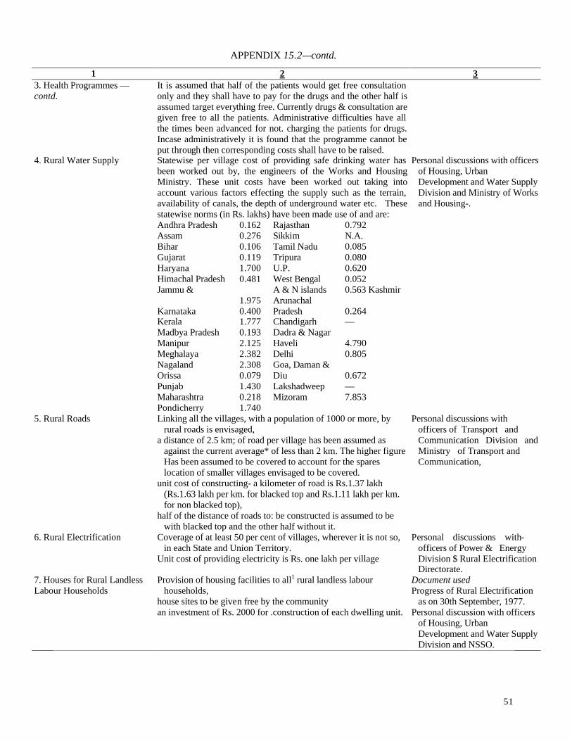
51


1 2 3 3. Health Programmes — contd.

It is assumed that half of the patients would get free consultation only and they shall have to pay for the drugs and the other half is assumed target everything free. Currently drugs & consultation are given free to all the patients. Administrative difficulties have all the times been advanced for not. charging the patients for drugs. Incase administratively it is found that the programme cannot be put through then corresponding costs shall have to be raised.

4. Rural Water Supply Statewise per village cost of providing safe drinking water has been worked out by, the engineers of the Works and Housing Ministry. These unit costs have been worked out taking into account various factors effecting the supply such as the terrain, availability of canals, the depth of underground water etc. These statewise norms (in Rs. lakhs) have been made use of and are: Andhra Pradesh 0.162 Rajasthan 0.792 Assam 0.276 Sikkim N.A. Bihar 0.106 Tamil Nadu 0.085 Gujarat 0.119 Tripura 0.080 Haryana 1.700 U.P. 0.620 Himachal Pradesh 0.481 West Bengal 0.052 Jammu & A & N islands 0.563 Kashmir 1.975 Arunachal Karnataka 0.400 Pradesh 0.264 Kerala 1.777 Chandigarh — Madbya Pradesh 0.193 Dadra & Nagar Manipur 2.125 Haveli 4.790 Meghalaya 2.382 Delhi 0.805 Nagaland 2.308 Goa, Daman & Orissa 0.079 Diu 0.672 Punjab 1.430 Lakshadweep — Maharashtra 0.218 Mizoram 7.853 Pondicherry 1.740

Personal discussions with officers of Housing, Urban Development and Water Supply Division and Ministry of Works and Housing-.

5. Rural Roads Linking all the villages, with a population of 1000 or more, by rural roads is envisaged,

a distance of 2.5 km; of road per village has been assumed as against the current average* of less than 2 km. The higher figure Has been assumed to be covered to account for the spares location of smaller villages envisaged to be covered.

unit cost of constructing- a kilometer of road is Rs.1.37 lakh (Rs.1.63 lakh per km. for blacked top and Rs.1.11 lakh per km. for non blacked top),

half of the distance of roads to: be constructed is assumed to be with blacked top and the other half without it.

Personal discussions with officers of Transport and Communication Division and Ministry of Transport and Communication,

6. Rural Electrification Coverage of at least 50 per cent of villages, wherever it is not so, in each State and Union Territory.

Unit cost of providing electricity is Rs. one lakh per village

Personal discussions with- officers of Power & Energy Division $ Rural Electrification Directorate.

7. Houses for Rural Landless Labour Households

Provision of housing facilities to all1 rural landless labour households,

house sites to be given free by the community an investment of Rs. 2000 for .construction of each dwelling unit.

Document used Progress of Rural Electrification

as on 30th September, 1977. Personal discussion with officers

of Housing, Urban Development and Water Supply Division and NSSO.

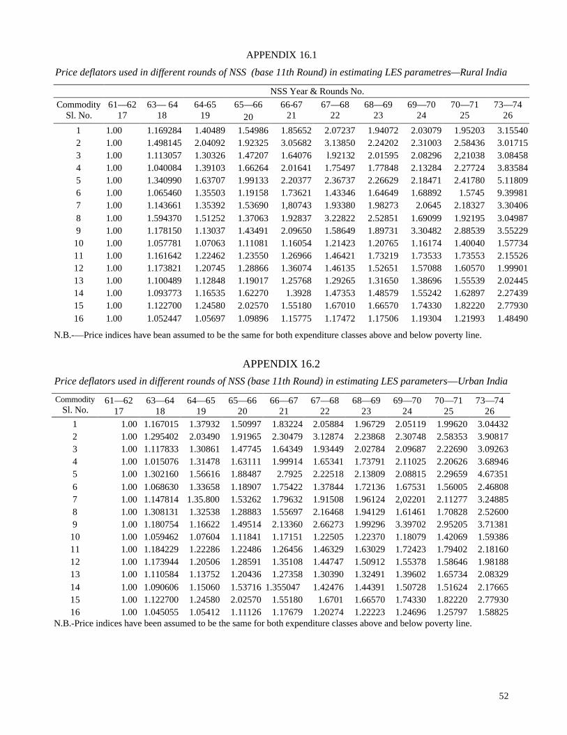
52

APPENDIX 16.1

Price deflators used in different rounds of NSS (base 11th Round) in estimating LES parametres—Rural India

NSS Year & Rounds No.

Commodity Sl. No.

61—62 17

63— 64 18

64-65 19

65—66 20

66-67 21

67—68 22

68—69 23

69—70 24

70—71 25

73—74 26

1 1.00 1.169284 1.40489 1.54986 1.85652 2.07237 1.94072 2.03079 1.95203 3.15540 2 1.00 1.498145 2.04092 1.92325 3.05682 3.13850 2.24202 2.31003 2.58436 3.01715 3 1.00 1.113057 1.30326 1.47207 1.64076 l.92132 2.01595 2.08296 2,21038 3.08458 4 1.00 1.040084 1.39103 1.66264 2.01641 1.75497 1.77848 2.13284 2.27724 3.83584 5 1.00 1.340990 1.63707 1.99133 2.20377 2.36737 2.26629 2.18471 2.41780 5.11809 6 1.00 1.065460 1.35503 1.19158 1.73621 1.43346 1.64649 1.68892 1.5745 9.39981 7 1.00 1.143661 1.35392 1.53690 1,80743 1.93380 1.98273 2.0645 2.18327 3.30406

8 1.00 1.594370 1.51252 1.37063 1.92837 3.22822 2.52851 1.69099 1.92195 3.04987 9 1.00 1.178150 1.13037 1.43491 2.09650 1.58649 1.89731 3.30482 2.88539 3.55229 10 1.00 1.057781 1.07063 1.11081 1.16054 1.21423 1.20765 1.16174 1.40040 1.57734 11 1.00 1.161642 1.22462 1.23550 1.26966 1.46421 1.73219 1.73533 1.73553 2.15526 12 1.00 1.173821 1.20745 1.28866 1.36074 1.46135 1.52651 1.57088 1.60570 1.99901 13 1.00 1.100489 1.12848 1.19017 1.25768 1.29265 1.31650 1.38696 1.55539 2.02445 14 1.00 1.093773 1.16535 1.62270 1.3928 1.47353 1.48579 1.55242 1.62897 2.27439 15 1.00 1.122700 1.24580 2.02570 1.55180 1.67010 1.66570 1.74330 1.82220 2.77930

16 1.00 1.052447 1.05697 1.09896 1.15775 1.17472 1.17506 1.19304 1.21993 1.48490

N.B.-—Price indices have bean assumed to be the same for both expenditure classes above and below poverty line.

APPENDIX 16.2

Price deflators used in different rounds of NSS (base 11th Round) in estimating LES parameters—Urban India

Commodity Sl. No.

61—62 17

63—64 18

64—65 19

65—66 20

66—67 21

67—68 22

68—69 23

69—70 24

70—71 25

73—74 26

1 1.00 1.167015 1.37932 1.50997 1.83224 2.05884 1.96729 2.05119 1.99620 3.04432 2 1.00 1.295402 2.03490 1.91965 2.30479 3.12874 2.23868 2.30748 2.58353 3.90817 3 1.00 1.117833 1.30861 1.47745 1.64349 1.93449 2.02784 2.09687 2.22690 3.09263 4 1.00 1.015076 1.31478 1.63111 1.99914 1.65341 1.73791 2.11025 2.20626 3.68946 5 1.00 1.302160 1.56616 1.88487 2.7925 2.22518 2.13809 2.08815 2.29659 4.67351

6 1.00 1.068630 1.33658 1.18907 1.75422 1.37844 1.72136 1.67531 1.56005 2.46808 7 1.00 1.147814 1.35.800 1.53262 1.79632 1.91508 1.96124 2,02201 2.11277 3.24885 8 1.00 1.308131 1.32538 1.28883 1.55697 2.16468 1.94129 1.61461 1.70828 2.52600 9 1.00 1.180754 1.16622 1.49514 2.13360 2.66273 1.99296 3.39702 2.95205 3.71381 10 1.00 1.059462 1.07604 1.11841 1.17151 1.22505 1.22370 1.18079 1.42069 1.59386 11 1.00 1.184229 1.22286 1.22486 1.26456 1.46329 1.63029 1.72423 1.79402 2.18160 12 1.00 1.173944 1.20506 1.28591 1.35108 1.44747 1.50912 1.55378 1.58646 1.98188 13 1.00 1.110584 1.13752 1.20436 1.27358 1.30390 1.32491 1.39602 1.65734 2.08329

14 1.00 1.090606 1.15060 1.53716 1.355047 1.42476 1.44391 1.50728 1.51624 2.17665 15 1.00 1.122700 1.24580 2.02570 1.55180 1.6701 1.66570 1.74330 1.82220 2.77930 16 1.00 1.045055 1.05412 1.11126 1.17679 1.20274 1.22223 1.24696 1.25797 1.58825

N.B.-Price indices have been assumed to be the same for both expenditure classes above and below poverty line.

53

TECHNICAL APPENDIX

Engel Curves I Demand functions

In the consumption model, the following five demand function forms have been used. Log Inverse and Log log Inverse forms could not be used as they were not integrable over the range of the log normal distribution for estimating the expected values

i) Double Log (DL) Log Ci=a+b log c2 f(c)=acb

ii) Semi Log (SL) f(c)=ci=a+b log c iii) Linear (L) f(c)= ci = a+b/c iv) Hyperbola (HYP) f(c) = ci =a+b/c v) Propensity (Proportion) (P) f(c)=ci=a.c

where

c = monthly per capita total consumption expenditure.

ci = monthly per capita expenditure on commodity i.

a,b = parameters of the estimated demand functions.

Best fitting Engel Curves among these were chosen separately for each commodity on the basis of highest value of corrected R-2 obtained by applying the single equation weighted least square method, the freights being the percentages of population in different expenditure classes.

Another two functions viz., log inverse and log log inverse, though found to be best in case of some commodities could not be used as the mathematical expressions for their expected valu-es could not be explicitly obtained under log normal distribution.

On the assumption that c is log normally dis-tributed with parameters M&λ , the following formula for each demand function form has been used to estimate the expected value of monthly per capita expenditure on commodity i, corres-ponding to the above demand functions.

where

∧ (C/M, λ2) is log normal distribution with parameters

M & λ where λ is same as that of 1973-74

and M=log C—λ2/2

Using (I) the expression for the expected value of commodity consumption have been derived and given below for each of the above types of demand functions.

where,

φ = Ordinate of Standard normal curve

=area under the standard normal curve

m' = (log m-M)/ λ

n' = (log n-M)/ λ

Case (i) For Population below the poverty line

In the above generalised formulae, the range of integration is form r to c* (the poverty line). is the threshold value of monthly per capital consumption expenditure at which consumption of commodity i starts.

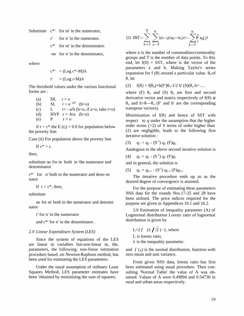
54

Substitute c*' for m' in the numerator,

r' for n' in the numerator.

c*' for m' in the denominator.

-oo for n' in the denominator,

where

c*' = (Log c*-M)/λ

r' = (Log r-M)/λ

The threshold values under the various functional forms are :

(a) DL r = o (b) SL r = e -a/b (b>o) (c) L r= - a/b (b>o, if a>o, take r=o) (d) HYP r = -b/a (b<o) (e) P r = o

if r > c* the E (ci) = 0.0 for population below the poverty line.

Case (it) For population above the poverty line

If c* > r.

then,

substitute oo for m both in 'the numerator and denominator

c*' for n' both in the numerator and deno-m nator

If r > c*, then,

substitute

oo for m' both in the numerator and denomi-nator

r' for n' in the numerator

and c*' for n' in the denominator .

2.0 Linear Expenditure System (LES)

Since the system of equations of the LES are linear in variables but-non-linear in, the, parameters, the following; non-linear estimation procedure based .on Newton-Raphson method, has been used for estimating the LES parameters:

Under the usual assumption of ordinary Least Squares Method, LES parameter estimates have been 'obtained by minimising the sum of squares:

where n is the number of commodities/commodity groups and T is the number of data points. To this end, let f(0) = SST, where is the vector of the parameters a and b. Making Taylor's series expansion for f (θ) around a particular value. θ0 of θ, let

(2) f(θ) = f(θo)+h(F')θo-1/2 h' (S)(θo h+ ....

where (F) θo and (S) θo are first and second derivative vector and matrix respectively of f(θ) at θo and h=θ—θo (F' and h' are the corresponding transpose vectors).

Minimisation of f(θ) and hence of SST with respect to θ under the assumption that the higher order terms (>2) of S terms of order higher than (2) are negligible, leads to the following first iterative solution :

(3) θ1 = θo - (S-1) θo (F)θo

Analogous to the above second iterative solution is

(4) θ2 = θ1 - (S-1) θ1 (F)θ1

and in general, the solution is

(5) θn = θn-1 - (S-1) θn-1 (F)θn-1

The iterative procedure ends up as as the desired degree of convergence is attained.

For the purpose of estimating these parameters NSS data for the rounds Nos.17-25 and 28 have been utilised. The price indices required for the purpose are given in Appendices 16.1 and 16.2.

3.0 Estimation of inequality parameter (A) of Lognormal distribution Lorenz ratio of lognormal distribution is given by

L=2 φ (λ // /−2 ) -1, where

L is lorenz ratio, λ is the inequality parameter.

and φ (X) is the normal distribution, function with zero mean and unit variance.

From given NSS data, lorenz ratio has first been estimated using usual procedure. Then con-sulting 'Normal Table' the value of A was ob-tained. Values of A were 0.49894 and 0.54730 in rural and urban areas respectively.

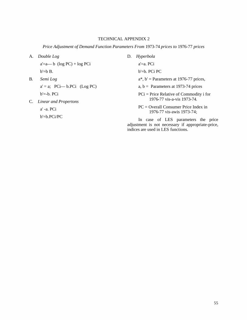
55

TECHNICAL APPENDIX 2

Price Adjustment of Demand Function Parameters From 1973-74 prices to 1976-77 prices

A. Double Log

a'=a— b (log PC) + log PCi

b'=b B.

B. Semi Log

a' = a; PCi— b.PCi (Log PC)

b'=-b. PCi

C. Linear and Propertons

a' -a. PCi

b'=b.PCi/PC

D. Hyperbola

a'=a. PCi

b'=b. PCi PC

a*, b' = Parameters at 1976-77 prices,

a, b = Parameters at 1973-74 prices

PCi = Price Relative of Commodity i for 1976-77 vis-a-vis 1973-74.

PC = Overall Consumer Price Index in 1976-77 vis-awis 1973-74;

In case of LES parameters the price adjustment is not necessary if appropriate-price, indices are used in LES functions.

56

ANNEXURE I

I(a) Comments of Prof. N. S. lyeugar

Indian Statistical Institute

Bangalore Centre

Dr. K. C. Majumdar. 31, Church Street, Chief (PP) Bangalore 560001. Planning Commission 19 April 1979 Yojana Bhavan, Parliament Street, New Delhi-1 10001

Dear Dr. Majumdar

Your letter 4/3/77-FP of March 13, 1979 has just arrived from Hyderabad, where it first want during my absence. Since I am attending your meeting on 23 April 1979, I shall make a few comments of a methodological nature at the meeting itself.

I am not too happy with the methodology of demand projections used in the report. I notice that individual commodities have been aggregated first into a smaller number of composite items, and a linear expenditure system is then hypothesised for the composite items ; this is a simple version of the more general model of Richard Stone, where time elements are also incorporated. The composite items are then split up into individual items by using one or more forms of Engel Curves. There is a real difficulty in appreciating the techniques followed here. For purposes of combining individual items into composite items, simple aggregation has been used to generate data, but the Engel curves actually used for individual items are not additive.

A more satisfactory formulation would be as follows. Let a constant level of living below which a certain proportion p of households are assumed to live ; this number is pre-determined by one or more considerations, involving value judgments and an accurate knowledge of prices and products. The proportion, p, can be estimated from the ogive of the distribution of x, income or its proxy, total outlay, given in NSS reports. The NSS also provides information for computing the specific concentration curves and the Lorenz curve, which in turn will enable one to compute the cumulative proportions, q0 arid Qi0 (1=1,2....), corresponding

to p0 where qc proportion of aggregate total outlay spent by the 'poor' and Qic = proportion of aggregate expenditure on an item 'i' incurred by the same 'poor', the poor being understood as the set of households having x< c.

Let g(x)— E(y/x) represent the conditional means of y for given x. This function represents the Engel. Curve of the given commodity in a strict sense. For items T let it be represented by gi (x). The following relationships hold :

E(x)/x≤c)=qc E(X1)/Pc

E(Yi/x≤c)=Qic E(yi)/P ic

Pc, qc, and Qic are readily available in empirical specific concentration curves and the Lorenz curve. Parametric forms for E(x/x≤c) and E(yi/x≤c) can be found if suitable assumptions can be made about the distribution of x and g(x) for different items. Suitable policy instruments can be devised in terms of those parameters.

Another point that often bothers me is; when the joint distribution of (x, Y1, Y2..........) can be assumed (e.g. joint lognormality), the Engel Curves are all once for all assumed. It does not make sense to think of different forms and use R2 to choose the best form.

I hope to learn from the discussions at the meeting. As on previous occasions, may I request you to arrange payment of TA (airfare) immediately after the meeting in Delhi itself?

Hoping to see you, and with regards,

Yours sincerely, Sd/- NS lyengar

57

I(b) Comments on the Remarks of: Prof. lyengar by Dr. R. Radhakrishtia I do not see much justification either on theore-tical or on empirical considerations in the remarks made by lyengar on the methodology ' adopted for demand projections, and his remarks appear to be rather misplaced in emphasis. Surprisingly his "more satisfactory formulation" is nothing but a simple and restrictive version of the formulation adopted by the, Task Force. For a proper appraisal of his remarks, it would be helpful to recapitulate the methodology as it appears lyengar is not fully familiar with the Task Force's formulation. In its initial meetings the Task Force decided to make the demand projections on the basis of a Complete Demand Model which satisfies the theoretical properties viz., adding-up homogeneity, Slutskly-symmetry and convexity and chose the most popular Linear Expenditure System (LES). There is considerable empirical support for this choice. The most recent is the research of Parks (1969), Pollack and Wales (1969), Yoshihara (1969), Coldberger and Gameletses (1970), Deaton (1974-1975), Lliich, Powell and Williams (1975) Radhakrishna and Murthy (1978), and Radhakrishna, Murthy and Shah (1979). Inci-dentally the last study has brought out the superiority of LES over Indirect Addilog and Quadratic Utility Functions in describing the consumption patterns of India. The. LES usually fulfils all the theoretical properties and gives a reasonably good fit. What is more, it aggregates perfectly over individuals in a group, given that each group member has the same utility functions — a property violated by most of the other demand models. The simple version of LES has been selected because the extensive studies carried out at Sardar Patel Institute have shown that it gives reasonably good fit when the range of expenditure variation is not very large. One could have introduced little more flexibility by introducing time trends (linear or quadratic or cubic or nth degree polinominal ! ) but the number of para-meters increases enormously. The studies at Sardar Patel Institute on mean level time series models with 4 to 9 commodity groups, where the time trend version of LES has an added advantage of handling the non-linearities, reveal no appreciable differences in the results given by the alternative versions of LES. Also, comparable NSS data with the required commodity grouping are available for a short period and some con-ceptional problems arise while estimating the alternative versions of LES as the data are time series of cross-section and the hypotheses are mostly developed for mean level models. Keeping in view the requirements of the income redistribution policies, the Task Force decided to. stratify the NSS expenditure classes into two groups :

one containing the classes below the poverty line and the other containing the rest, and lit LES separately for each group. This also overcomes the limitation of Linear Engel Curves implied by LES. Taking into consideration the availability of data and also the fact that the additive utility' specification implied by "LES is unrealistic at a disaggregated level of commodity grouping, the Task Force decided to estimate LES with 16 commodity groups. I emphasize here that the data consideration act as a constraint for enlarging the number of commodity groups. By integrating the LES with two parameter log-normal distribution, which has been hypothesized for the expenditure distribution, it will be possible to make demand projections under alternative assumptions about the expenditure distribution. This is exactly what the Task Force has done. In the above formulation ;if one considers Engel Curves in place of Complete Demand Models, the procedure will coincide with the one suggested by lyengar. It is obvious that the Task Force's formulation is more flexible and superior. I really fail to see violation of any theoretical property one should worry about. Let me now turn to the prediction of individual items within a group. It is well known that one should estimate sub-group models and use them to allocate the group expenditure to their components. (See in this connection Deaton (1975)]. However, the available data do not permit, us to estimate the sub-group models. The only alternative we are left with is to use some budget proportions. The Task Force has not adopted the conventional procedure of using the same proportion across all expenditure groups as it involves the very unrealistic assumption of homothetic partial indifference surfaces for subgroups and instead it has allowed the budget proportions to vary across the expenditure groups. The proportions are based on Engle Curves. Since the group expenditures given by LES are taken as group controls and the group expenditures are then allocated to their specific components by means of proportion, the adding up property is automatically fulfilled. The formulation based on Engel Curves suggested by lyengar is no doubt preferred in 1950s but it is not preferred any longer. The formulation ignores the variations in prices. Even in price-exogenous (fixed price) planning models, in order to make projections using Engel Curves, the price structure of the base period should be the same as that of the family budget survey. Incidentally, lyengar's procedure is no different from the one the Task Force has adopted while arriving at the budget proportions needed for splitting the group expenditures. Coming to his last point, I may draw his attention to the fact that in the Task Force formulation, only the total expenditure is assumed to be distributed as log-normal.

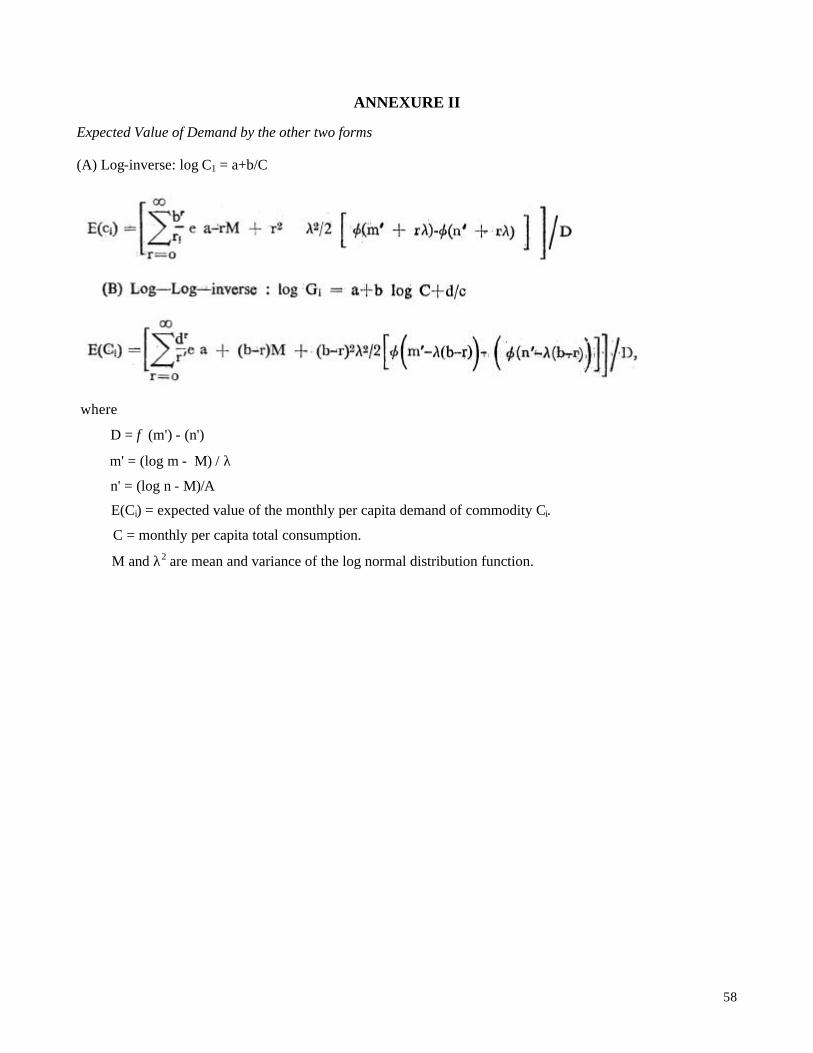
58

ANNEXURE II

Expected Value of Demand by the other two forms

(A) Log-inverse: log C1 = a+b/C

where

D = φ (m') - (n')

m' = (log m - M) / λ

n' = (log n - M)/A

E(Ci) = expected value of the monthly per capita demand of commodity Ci.

C = monthly per capita total consumption.

M and λ2 are mean and variance of the log normal distribution function.