minimizing technical risks in photovoltaic … minimizing technical risks in photovoltaic projects...
TRANSCRIPT

Minimizing Technical Risks in Photovoltaic Projects
Recommendations for Minimizing Technical Risks of PV Project Development and PV Plant Operation
Merged Deliverable D1.2 and D2.2 (M16)
2
Minimizing Technical Risks in Photovoltaic Projects
Foreword
The photovoltaic (PV) sector has overall experienced a significant growth globally in the last
decade, reflecting the recognition of PV as a clean and sustainable source of energy. Project
investment has been and still is a primary financial factor in enabling sustainable growth in PV
installations. When assessing the investment-worthiness of a PV project, different financial
stakeholders such as investors, lenders and insurers will evaluate the impact and probability of
investment risks differently depending on their investment goals. Similarly, risk mitigation measures
implemented are subject to the investment perspective. In the financing process, the stakeholders
are to elect the business model to apply and be faced with the task of taking appropriate
assumptions relevant to, among others, the technical aspects of a PV project for the selected
business model.
The Solar Bankability project aims to establish a common practice for professional risk
assessment which will serve to reduce the risks associated with investments in PV
projects. The risks assessment and mitigation guidelines are developed based on market data
from historical due diligences, operation and maintenance records, and damage and claim reports.
Different relevant stakeholders in the PV industries such as financial market actors, valuation and
standardization entities, building and PV plant owners, component manufacturers, energy
prosumers and policy makers are engaged to provide inputs to the project.
The technical risks at the different phases of the project life cycle are compiled and quantified
based on data from existing expert reports and empirical data available at the PV project
development and operational phases. The Solar Bankability consortium performs empirical and
statistical analyses of failures to determine the manageability (detection and control), severity, and
the probability of occurrence. The impact of these failures on PV system performance and energy
production are evaluated. The project then looks at the practices of PV investment financial models
and the corresponding risk assessment at present days. How technical assumptions are accounted
in various PV cost elements (CAPEX, OPEX, yield and performance ratio) are inventoried.
Business models existing in the market in key countries in the EU region are gathered. Several
carefully selected business cases are then simulated with technical risks and sensitivity analyses
are performed.
The results from the financial approaches benchmarking and technical risk quantification are used
to identify the gaps between the present PV investment practices and the available extensive
scientific data in order to establish a link between the two. The outcomes are best practices
guidelines on how to translate important technical risks into different PV investment cost elements
and business models. This will build a solid fundamental understanding among the different
stakeholders and enhance the confidence for a profitable investment.
The Solar Bankability consortium is pleased to present this report which is one of the public
deliverables from the project work.

3
Minimizing Technical Risks in Photovoltaic Projects
Other Publications from the Solar Bankability
Consortium
Description Publishing date
Snapshot of Existing and New Photovoltaic Business Models August 2015
Technical Risks in PV Project Development and PV Plant Operation
March 2016
Review and Gap Analyses of Technical Assumptions in PV Electricity Cost
July 2016
Minimizing Technical Risks in Photovoltaic Projects August 2016
Financial Modelling of Technical Risks in PV Projects September 2016
Best Practice Guidelines for PV Cost Calculation December 2016
Technical Bankability Guidelines February 2017
Proceedings from the Project Advisory Board and
from the Public Workshops
Description Publishing date
1st Project Advisory Board closed meeting June 2015
2nd Project Advisory Board closed meeting December 2015
First Public Solar Bankability Workshop - Enhancement of PV Investment Attractiveness
July 2016
3rd Project Advisory Board closed meeting February 2017
Solar Bankability Final Workshop - Improving the attractiveness of solar PV investment
February 2017

4
Minimizing Technical Risks in Photovoltaic Projects
Principal Authors
Ulrike Jahn, Magnus Herz, Erin Ndrio (TUV-RH)
David Moser, Giorgio Belluardo (EURAC)
Mauricio Richter, Caroline Tjengdrawira (3E)
Acknowledgements
The Solar Bankability Consortium would like to extend special thanks to the Members of the Project’s
Advisory Board for their input and support: 123 Ventures, Deutsche Bank, Fronius, HSH-Nordbank, KGAL,
Naturstrom, SEL Spa, Solarcentury, Triodos Bank, WHEB group.
Project Information
EC Grant Agreement Number: No 649997
Duration: March 2015 until February 2017 (24 months)
Coordinator: EURAC Institute for Renewable Energy (IT)
Project Partners: 3E N.V. (BE), ACCELIOS Solar GmbH (DE), SolarPower Europe (BE), and TÜV Rheinland
Energy GmbH (DE)
Disclaimer
The sole responsibility for the content of this publication lies only with the authors. It does not necessarily
reflect the opinion of the European Communities. The European Commission is not responsible for any use
that may be made of the information contained therein.
5
Minimizing Technical Risks in Photovoltaic Projects
Table of Contents
FOREWORD ..................................................................................................................... 2
TABLE OF CONTENTS .................................................................................................................. 5
FIGURES & TABLES ..................................................................................................................... 6
GLOSSARIES & ABBREVIATIONS ................................................................................................ 8
EXECUTIVE SUMMARY ................................................................................................................ 9
1 INTRODUCTION ON MITIGATION MEASURES .............................................................. 14
2 DESCRIPTION OF CATEGORIES OF MITIGATION MEASURES .................................... 18 2.1 CAPEX related Mitigation Measures and Preventive Measures ......................................... 19 2.1.1 Design Verification and Description of Mitigation Measures ............................................... 19 2.2 OPEX related Mitigation Measures and Corrective Measures ............................................ 21 2.2.1 Operation & Maintenance .................................................................................................. 22
3 FACT SHEETS FOR MITIGATION MEASURES ............................................................... 23 3.1 Parameters of the Fact Sheet ............................................................................................ 23
4 METHODOLOGY .............................................................................................................. 30 4.1 Definition of Best and Worst Uncertainty Scenarios ........................................................... 30 4.2 CPN Reduction by Different Mitigation Measures .............................................................. 41 4.3 Critical Aspects of the Proposed Approaches .................................................................... 43 4.3.1 Error Propagation in Yield Uncertainty for Failures during Planning ................................... 43 4.3.2 CPN methodology and mitigation measures ...................................................................... 44
5 ANALYSIS AND RESULTS ............................................................................................... 44 5.1 Impact on Initial Energy Yield Prediction and Exceedance Probability for the Defined
Scenarios with Reduced Uncertainties .............................................................................. 44 5.2 Impact of Applied Mitigation Measures on and Ranking of CPN ........................................ 48 5.2.1 Mitigation measures applied to the FIX scenario ................................................................ 52 5.2.2 Mitigation measures applied to the LOSS scenario ............................................................ 54 5.3 Risk Reduction Example (PID) before Detection................................................................ 58
6 RISK REDUCTION AND LINK TO GAP ANALYSIS .......................................................... 60
7 CONCLUSIONS ................................................................................................................ 62
REFERENCES ................................................................................................................... 65
APPENDICES ................................................................................................................... 67
ANNEX 1: LIST OF ALL MITIGATION MEASURES WITH DESCRIPTION .................................. 67
ANNEX 2: LIST OF IMPACT OF APPLIED MITIGATION MEASURES ON RISKS ....................... 69
ANNEX 3: INDEX OF ALL COMBINATIONS ................................................................................ 70
ANNEX 4: UNCERTAINTY VALUES OF INPUT AND OUTPUT PARAMETERS IN THE DIFFERENT UNCERTAINTY SCENARIOS .................................................................................. 74
ANNEX 5: EXAMPLES OF UNCERTAINTY REDUCTION IN THE YIELD ASSESSMENT ........... 75
6
Minimizing Technical Risks in Photovoltaic Projects
Figures & Tables
Table 2.1: The factor of 10 applied in PV plants. Every phase of the plant has a different cost factor regarding the same failure ....... 20 Table 2.2: Example of a failure due to wrong sizing of the inverters and the financial impact (Klute, 2016) ....................................... 20 Table 3.1: Fact Sheet on Mitigation Measure - Component Testing – PV Modules .............................................................................. 24 Table 3.2: Fact Sheet on Mitigation Measure – PV Plant Planning ....................................................................................................... 25 Table 3.3: Fact Sheet on Mitigation Measure - Design Review and Construction Monitoring ............................................................. 27 Table 3.4: Fact Sheet on Mitigation Measure – Basic and Advanced Monitoring System .................................................................... 28 Table 3.5: Fact Sheet on Mitigation Measure – Reducing Uncertainties (Irradiance) ........................................................................... 29 Table 4.1: Main characteristics and settings of the simulated PV system in Bolzano ........................................................................... 34 Table 4.2: Parameters describing the frequency distribution of the errors of the input parameters used for the 1000 simulations with
PVSyst. Only the base uncertainty case scenario is reported. ................................................................................................................ 34 Table 4.3: List of uncertainties assumed for the different input parameters, both in the base uncertainty scenario and in the alternative
uncertainty scenarios ............................................................................................................................................................................. 39 Table 4.4: Ranking list of the base and alternative uncertainty scenarios based on the calculated value of uncertainty on the final yield
of the 4 kWp PV system installed in Bolzano ....................................................................................................................................... 40 Table 5.1: Summary of the exceedance probability values for various scenarios .................................................................................. 47 Table 5.2: List of most significant measures, their mitigation factors and affected parameters ............................................................ 49 Table 5.3: List of mitigation measures with medium, low and high cost scenarios ............................................................................... 50 Table 5.4: Definition of impact classes with respect to risk mitigation factor (RMF) ........................................................................... 51 Table 5.5: Example of combination of mitigation measures.................................................................................................................. 51 Table 5.6: Best combinations of mitigation measures for medium (1), low (2) and high (3) cost scenarios and their savings in CPN
(last column) .......................................................................................................................................................................................... 53 Table 5.7: Combination of mitigation measures for the defined LOSS scenarios ................................................................................. 55 Table 5.8: Combination of mitigation measures for the defined LOSS scenarios ................................................................................. 57 Table 5.9: Input Data for Risk Reduction Example (PID) ..................................................................................................................... 58 Table 5.10: Output Data for Risk Reduction Example (PID) after 0 to 5 Years .................................................................................... 58 Table 6.1: Punch list of technical aspects to be considered in the EPC and O&M contracts ................................................................. 61
Figure 1.1: Example of failure flows along the value chain of a PV project for some module related technical risks. The number
relates to the list of technical risks as presented in the Report (Moser et al., 2016)............................................................................... 15 Figure 4.1: List of the risks having an economic impact in terms of uncertainty of either estimated or actual yield of a PV plant.
Numbers are taken from the list of risks presented in (Moser et al., 2016) ........................................................................................... 31 Figure 4.2: General schematic of a model for the estimation of the yield of a PV system. Risks generating uncertainty are reported
with a representative value of associated uncertainty, and colored depending on the related component. Mutual influences are
indicated by arrows. ............................................................................................................................................................................... 32 Figure 4.3: Frequency distribution and cumulative frequency distribution of the parameters array yield (Ya), final yield (Yf) and
performance ratio (PR), generated from 1000 simulations with PVSyst using input parameters errors distributed according to Table
4.2. Red line represents the corresponding normal distribution with empirical mean (μ) and standard deviation (σ). Only the base
uncertainty scenario is represented. ....................................................................................................................................................... 35 Figure 4.4: Propagation of the uncertainty from the simulation software (PVSyst) input to the different output parameters, using the
Monte Carlo technique and the rule of square. Only the base uncertainty scenario is considered. ........................................................ 35 Figure 5.1: Comparison of the cumulative distribution function for a normal distribution with σ=4.6% (k=1) (black curve) and the
results from a Monte Carlo analysis (red curve) .................................................................................................................................... 45 Figure 5.2: Comparison of the three scenarios assuming a normal distribution .................................................................................... 46 Figure 5.3: Comparison of the worst case scenario with different mean values of the normal distribution with σ=16.6% ................... 47 Figure 5.4: Top 10 risks of PV modules with and without mitigation measures in CPN ....................................................................... 51 Figure 5.5. Top 10 risks of inverter with and without mitigation measures in CPN .............................................................................. 52

7
Minimizing Technical Risks in Photovoltaic Projects
Figure 5.6: New CPN results of mitigation measure combinations for different FIX cost scenarios compared to CPN without MM –
Index of mitigation measure combinations is given in Annex 3. ........................................................................................................... 53 Figure 5.7: New CPN results of mitigation measure combinations of different LOSS scenarios based on high PPA compared to CPN
without mitigation measures .................................................................................................................................................................. 55 Figure 5.8: New CPN results of mitigation measure combinations of different LOSS scenarios based on Low PPA compared to CPN
without mitigation measures .................................................................................................................................................................. 56 Figure 5.9: LOSS Scenario – PID Risk Reduction after 0 to 5 Years .................................................................................................... 59 Figure A5.1: Impact of mitigation measures compared to the base scenario (fixed at 0) ...................................................................... 75 Figure A5.2: Typical values of uncertainty reduction in relative terms for a few selected mitigation measures ................................... 75 Figure A5.3: Example of uncertainty reduction (in relative terms) for a scenario where long term series of measured data on the plane
of array are available (low-end scenario) ............................................................................................................................................... 76 Figure A5.4: Example of uncertainty reduction (in relative terms) where long term series of satellite data are combined with short
term series of measured data.................................................................................................................................................................. 76

8
Minimizing Technical Risks in Photovoltaic Projects
Glossaries & Abbreviations
CDF Cumulative Distribution Function
CPN Cost Priority Number
DiffHI Diffuse Horizontal Irradiance
EPC Engineering Procurement and Construction
EL Electroluminescence imaging
EYP Energy Yield Prediction
FiT Feed-In Tariff
FMEA Failure Modes and Effects Analysis
GHI Global Horizontal Irradiance
GTI Global Tilted Irradiance
IEA International Energy Agency
IR Infrared imaging
LCOE Levelised Cost of Electricity
O&M Operation & Maintenance
PLR Performance Loss Rate
POA Plane of Array
PPA Power Purchasing Agreement
PR Performance Ratio
PV Photovoltaic
PVPS Photovoltaic Power Systems Programme
RCE Retail Cost of Electricity
RPN Risk Priority Number
RMF Risk Mitigation Factor
STC Standard Test Conditions

9
Minimizing Technical Risks in Photovoltaic Projects
Executive Summary
In the project report “Technical Risks in PV Projects” (Moser et al., 2016), technical risks were
identified and categorised for components and phases of the value chain of a PV project. The
technical risks were broadly divided into risks to which one can assign an uncertainty to the initial
yield assessment and risks to which one can assign a Cost Priority Number (CPN). While failures
arising from technical risks belonging to the first group have an impact on the overall uncertainty of
the energy yield, failures with a CPN have a direct impact on the annual cost of running a PV plant
caused by economic losses due to downtime (utilisation factor) and component repair or
substitution (OPEX) and it is given in Euros/kWp or Euros/kWp/year. The CPN methodology was
thus developed to assess the economic impact of technical risks occurring during the operation
and maintenance phase (O&M) of a PV project. The analysis summarized in the report “Technical
Risks in PV Projects” was linked to a failure database over a portfolio of more than 700 PV plants,
420 MWp, ~2,000,000 modules, ~12,000 inverters, etc. for a total of ~2.4 million components
(status March 2016). Although the database already includes PV plants from various market
segments and countries, the comparison of the CPNs for various technical risks (e.g. quantifiable
failures during O&M) was carried out on an annual basis for all plants. This is a shortcoming of the
database and not of the methodology.
The overall methodology was created to allow the estimation of the economic impact of failures on
the levelized cost of electricity (LCOE) and on business models of PV projects. Not all the technical
risks fit into the two groups mentioned above: some risks can be defined as precursor of a risk
propagating along the value chain or have an indirect impact on the CPN of various risks in terms
of occurrence, time to detect, time to repair, etc. Thus, the overall technical risk framework in the
Solar Bankability project has been developed to determine the economic impact of a failure but
also to be able to assess the effectiveness of mitigation measures.
Mitigation measures must be identified along the value chain and assigned to various technical
risks. Some failures can be prevented or mitigated through specific actions at different project
phases as, for e.g., for potential induced degradation (PID) the use of a different encapsulant or
glass during the product manufacturing phase, or a PID box in case of reversible PID during the
operation/maintenance phase. Others can be prevented or mitigated through a more generic
action. For example, the monitoring of performance or visual inspection can be considered as
generic mitigation measures that can have a positive impact on the reduction of the CPN of many
failures. In practice, it is important to understand how mitigation measures can be considered as a
whole to be able to calculate their impact and thus assess their effectiveness.
It is not the aim of this report to provide a set of specific mitigation measure for each technical risk
as this would entail failure specific cost-benefit analysis. At this stage, the Solar Bankability project
objective is to create a framework of well-defined mitigation measures, which have an impact on
the global CPN (given as sum of CPNs of all technical risks). The cost-benefit analysis can then
10
Minimizing Technical Risks in Photovoltaic Projects
include the combination of various mitigation measures and derive the best strategy depending on
market segment and plant typology. In addition to this, it is important to assess in the CPN analysis
who bears the cost and the risk to derive considerations not only on the overall economic impact of
the technical risks, but also on cost and risk ownership.
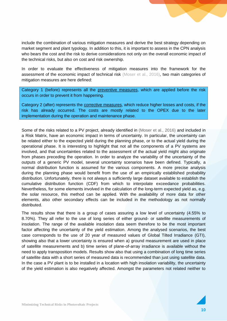
In order to evaluate the effectiveness of mitigation measures into the framework for the
assessment of the economic impact of technical risk (Moser et al., 2016), two main categories of
mitigation measures are here defined:
Category 1 (before) represents all the preventive measures, which are applied before the risk
occurs in order to prevent it from happening.
Category 2 (after) represents the corrective measures, which reduce higher losses and costs, if the
risk has already occurred. The costs are mostly related to the OPEX due to the later
implementation during the operation and maintenance phase.
Some of the risks related to a PV project, already identified in (Moser et al., 2016) and included in
a Risk Matrix, have an economic impact in terms of uncertainty. In particular, the uncertainty can
be related either to the expected yield during the planning phase, or to the actual yield during the
operational phase. It is interesting to highlight that not all the components of a PV systems are
involved, and that uncertainties related to the assessment of the actual yield might also originate
from phases preceding the operation. In order to analyze the variability of the uncertainty of the
outputs of a generic PV model, several uncertainty scenarios have been defined. Typically, a
normal distribution function is assumed for the various components. A more precise analysis
during the planning phase would benefit from the use of an empirically established probability
distribution. Unfortunately, there is not always a sufficiently large dataset available to establish the
cumulative distribution function (CDF) from which to interpolate exceedance probabilities.
Nevertheless, for some elements involved in the calculation of the long-term expected yield as, e.g.
the solar resource, this method can be applied. With the availability of more data for other
elements, also other secondary effects can be included in the methodology as not normally
distributed.
The results show that there is a group of cases assuring a low level of uncertainty (4.55% to
8.70%). They all refer to the use of long series of either ground- or satellite measurements of
insolation. The range of the available insolation data seem therefore to be the most important
factor affecting the uncertainty of the yield estimation. Among the analysed scenarios, the best
case corresponds to the use of 20 year of measured values of Global Tilted Irradiance (GTI),
showing also that a lower uncertainty is ensured when a) ground measurement are used in place
of satellite measurements and b) time series of plane-of-array irradiance is available without the
need to apply transposition models. Results show also that using a combination of long time series
of satellite data with a short series of measured data is recommended than just using satellite data.
In the case a PV plant is to be installed in a location with high insolation variability, the uncertainty
of the yield estimation is also negatively affected. Amongst the parameters not related neither to

11
Minimizing Technical Risks in Photovoltaic Projects
insolation variability nor to solar resource, the uncertainty related to shading and soiling effects,
and to the use of the right transposition model, plays a role in the uncertainty of the final yield. In
general, the uncertainty of the final yield of the PV plant used in the analysis can range from 4.5%
to 14.9%. The latter becomes a 16.6% in the eventuality that the planner has the worst information
quality available.
The cumulative distribution functions are shown in the figure below for the low-end scenario
(σ=4.6%), a high-end scenario (σ=9.3%) and the worst-case scenario (σ=16.6%).
The use of shorter time series can also lead to an underestimation (or overestimation) of the mean
specific value depending if the tails of the distribution are present or not. As an example, when
compared to a low-end scenario (4.6% uncertainty), the reduction in P90 for the worst-case
scenario (16.6% uncertainty and underestimation of the mean specific energy yield value) is 22%
(see Figure below).
Besides the technical risks associated with uncertainties during project planning phase, the second
group of risks has a direct economic impact during operation. These risks were already identified
and evaluated in (Moser et al., 2016). The methodology of quantification was also introduced in

12
Minimizing Technical Risks in Photovoltaic Projects
chapter 5 of the mentioned report and the results were based on two different scenarios: i) a FIX
scenario and ii) a never detected scenario. The overall sum of the CPNs for all components was
around 120 Euros/kWp/year.
The methodology has been further developed for the evaluation and effectiveness of the identified
mitigation measures. Risk Mitigation Factors (RMF) are introduced which quantify the reduction of
costs for fixing the failures (i.e. repair of existing component, substitution by spare component,
substitution by new component).
The new CPN (CPNnew) value arise from the cost-benefit analysis by adding the CPN after
mitigation with the cost of the mitigation measures. The Figure below shows the results of
calculating the FIXING costs for selected failures when applying combinations of eight selected
mitigation measures listed in Table 5.3. The index of 256 combinations can be found in Annex 3.
The costs related to FIXING the failures result from the sum of the costs of repair/substitution, the
costs of detection, the costs of transport, and the cost of labour. The selection of failures was
based on experts’ panels and include the top 20 PV module failures, top 20 inverter failures,
failures of mounting structure, combiner boxes, cabling as well as failures of transformer station as
listed in Annex 2 of this report.
Preventive measures have the highest impact on CPNnew e.g. Qualification of EPC will bring down
CPNnew to 75 €/kwp/year. E.g. Design review will further reduce to CPNnew to 40 €/kwp/year.
Corrective measures have less impact on CPNnew e.g. Basic and advanced monitoring and visual
and advanced inspection. In general, mitigation measures which reduce the failure occurrence
have the highest impact due to the related reduction in substitution costs. For 99% of all mitigation
measure combinations the scenarios will result in economic benefit by reducing the CPNnew to
values lower than the reference one (104.75 €/kWp/year) as shown in the Figure above. The
highest savings for all three cost scenarios can be achieved by applying the three preventive
measures (component testing + design review + qualification of EPC). The savings may reach
90 €/kWp/year for the best combinations of selected mitigation measures.

13
Minimizing Technical Risks in Photovoltaic Projects
The report presents the results of the identification and categorisation of mitigation measures
before and after the operational phase of a PV project.
In Chapter 2, two main categories for the description of mitigation measures are introduced
together with their relation to CAPEX and OPEX.
In Chapter 3, several fact sheets describe specific mitigation measures, their cost and the impact.
In Chapter 4, we describe the methodology used to assess the impact for mitigation measures
affecting technical risks related to the uncertainty of the energy yield and technical risks to which
we can assign a CPN. The methodology for the calculation of the CPN is extended to include the
impact of preventive and corrective mitigation measures.
In Chapter 5, the results of the analysis are given together with a prioritization of mitigation
measures.
Finally, Chapter 6 describes the link of the present report with the work carried out within the Solar
Bankability project in terms of gap analysis and impact on the LCOE and on the business models.

14
Minimizing Technical Risks in Photovoltaic Projects
1 Introduction on Mitigation Measures
In the project report “Technical Risks in PV Projects” (Moser et al., 2016), technical risks were
identified and categorised for components and phases of the value chain of a PV project. The
technical risks were broadly divided into risks to which one can assign an uncertainty to the initial
yield assessment and risks to which one can assign a Cost Priority Number (CPN). While failures
arising from technical risks belonging to the first group have an impact on the overall uncertainty of
the energy yield, failures with a CPN have a direct impact on the annual cost of running a PV plant.
The latter are caused by economic losses due to downtime (reduction in the utilisation factor) and
component repair or substitution (Operational Expenditures, OPEX) and it is given in Euros/kWp or
Euros/kWp/year. The CPN methodology was thus developed to assess the economic impact of
technical risks occurring during the operation and maintenance (O&M) phase of a PV project. The
analysis presented in the report “Technical Risks in PV Projects” was linked to a failure database
over a portfolio of more than 700 PV plants, 420 MWp, ~2,000,000 modules, ~12,000 inverters,
etc. for a total of ~2.4 million components (status March 2016). Although the database already
includes PV plants from various market segments and countries, the comparison of the CPNs for
various technical risks (e.g. quantifiable failures during O&M) was carried out on an annual basis
for all plants. This is a shortcoming of the database and not of the methodology. In fact, the
methodology already allows for the following analysis (among others):
- Market segment analysis (e.g. residential, commercial, industrial, utility scale)
- PV plants at different climates
- Differentiation between module type (e.g. crystalline silicon vs thin-film)
- Differentiation between inverter type (e.g. centralised vs string inverter)
- PV in different countries (e.g. labour costs)
- Distribution of failures over the years
- Assignment of an exceedance probability to the CPN (e.g. by using the energy yield at P50
or P90)
- Assessment of the economic impact of mitigation measures (e.g. reduction of failure
occurrence and time to detect).
The overall methodology was created to allow the estimation of the economic impact of failures on
the levelised cost of electricity (LCOE) and on business models of PV projects. Not all the technical
risks fit into these two groups: some risks can be defined as precursor of a risk propagating along
the value chain or have an indirect impact on the CPN of various risks in terms of occurrence, time
to detect, time to repair, etc. Thus, the overall technical risk framework in the Solar Bankability
project has been developed to determine the economic impact of a failure, but also to be able to
assess the effectiveness of mitigation measures. To this extent, it is important as a next step to
create failure flow maps to understand how failures propagate, to check for consistency, to assign

15
Minimizing Technical Risks in Photovoltaic Projects
liabilities, identify mitigation measures and assess their effectiveness in terms of reduction of
uncertainties and CPNs.
In a PV project, costs for correction of defects increase exponentially with a factor of 10 by each
step along the value chain from the product idea to the handover to the customer (Klute, 2016).
Defect prevention instead of defect correction should thus be considered as a first mitigation option
with an effective risk management strategy during system design and planning. The reduction in
occurrence of failures during the planning phase has in fact a direct positive consequence in terms
of reduction in occurrence of failures during the operational phase, resulting in a lower CPN.
Mitigation measures as defect correction will also have a cost. Therefore, the balance between the
increased capital expenditure during planning must be countered by an effective decrease of
operational (monetary) losses caused by downtime, component replacement or repair. It is
important to this extent to analyse how risks propagate from one step of the value chain to the
next: this allows us to identify mitigation measures and to understand if, for some specific failures,
an effective mitigation measure is already in place (see Figure 1.1). For the latter, it means that a
failure present during an early step of the value chain is not detected during the operational phase.
Figure 1.1: Example of failure flows along the value chain of a PV project for some module related technical risks. The number
relates to the list of technical risks as presented in the Report (Moser et al., 2016)
Typically, during the design of a PV project, a component qualification process is put in place. This
is applicable for the main components (module, inverter, mounting structure) and contains
16
Minimizing Technical Risks in Photovoltaic Projects
compatibility check, risk analysis, supplier audit, and lessons learnt. It entails different complexity
according to the project configuration (e.g. technology, country, region, climate).
As previously mentioned, the cost of mitigation measures needs to be included in a cost benefit
analysis, which has to consider the expectations of the stakeholders that are involved in a PV
project (Bächler, 2016). Investors are seeking for long defect warranty periods, performance
guarantees, reasonable low CAPEX and OPEX, high long-term plant performance and lifetime
(ideally above the initial prediction). Banks have requirements similar to those of the investors
which are looking for projects with a 10-15 year financing period and PV plant performance which
can also be slightly below prediction. Insurers try to limit their liability to failures with an external
root cause based on PV plants, which meet technical market standards and are maintained on a
regular basis. On the contrary, EPC contractors will look for short defect warranty periods,
minimum of additional guarantees and warranties, high sale price with low OPEX showing a very
different time horizon compared to the investors.
As a consequence of the different needs between the key actors, O&M operators are in a difficult
position to manage all these conflicting requirements for a long period of time. The best condition
for O&M operators is in fact in the presence of long defect warranty period and low sale price to
allow for higher OPEX. Recent trends in the PV market have put a lot of pressure on the O&M
price which is reported to be as low as 8 Euros/kWp/year in Germany in 2016 (Bächler, 2016). A
large share of these costs is labour intensive (i.e. site keeping and inspection, preventive
maintenance, monitoring and reporting). It is therefore of extreme importance to identify what
O&M scope is obligatory vs what is optional and the required reaction time depending on the
severity of the failure by assessing the cost of various mitigation options during the operational
phase which can be part of an effective O&M strategy.
Mitigation measures must be identified along PV the value chain and assigned to various technical
risks. Typical mitigation measures during the design phase are linked to the component selection
(e.g. standardised products, products with known track record), O&M friendly design (e.g.
accessibility of the site, state of the art design of the monitoring system), LCOE optimised design
(e.g. tracker vs. fixed tilt, central vs. string inverter, quality check of solar resource data). Mitigation
during the transportation and installations are linked to the supply chain management (e.g. well
organised logistics, quality assurance during transportation), quality assurance (e.g. predefined
acceptance procedures), grid connection (e.g. knowledge of grid code) (Herzog, 2016). These
mitigation measures positively affect the uncertainty of the overall energy yield, increase the initial
energy yield and reduce the cost of O&M during the operational phase (e.g. faster replacement of
components, lower cost of site maintenance, lower occurrence and severity of defect, etc.).
Mitigation measures during the O&M phase are linked to maintenance (e.g. preventive
maintenance, visual inspection, spare parts management), monitoring and data quality (e.g. state
of the art measurement equipment and software, performance evaluation, predictive monitoring),
outsourcing (e.g. in-sourcing can reduce costs and dependency from suppliers), remote monitoring
(e.g. video surveillance, defined workflow to reduce replacement time). These mitigation measures

17
Minimizing Technical Risks in Photovoltaic Projects
directly affect the CPN of failures occurring during the operational phase by reducing the time to
detect defects, the time to repair/substitute defects, etc.
Compared to many other power generating technologies, PV plants have reduced maintenance
and service requirements. However, a continuous O&M programme is essential to optimise energy
yield and maximise the lifetime and viability of the entire plant and its individual components. Many
aspects of O&M practices are interrelated and significantly affect the performance of all the
components in the generation chain and project lifecycle. The PV technical risks were defined in
the Project Report “Technical Risks in PV Projects” (Moser et al., 2016) in terms of downtime,
production performance, operational costs and time to complete the required activities. It is
important that risk ownership is also considered to better understand which key actor is
responsible for the action of mitigating the risk. These risks can then be turned in opportunities to
meet or even exceed the expectations of the developers and owners in terms of return on the
investment. In particular, suitable planning, supervision and quality assurance actions are critical at
all stages of a PV project in order to minimise the risk of damages and outages, optimise the use of
warranties, avoid non optimal use of resources and ultimately optimise the overall performance of
the PV plant.
The scientific PV community has thoroughly investigated some specific failures and drawn
recommendations on how to mitigate the economic impact for, e.g. soiling (Bengt Stridh, 2012;
Mani and Pillai, 2010; Qasem, 2013), grid integration (Appen et al., 2013), PID (Pingel et al.,
2010). General recommendations on the mitigation measures to reduce the impact of technical
risks are also found in more general publications given by companies active in the field as EPC
contractors, consultants, and O&M operators (Iban Vendrell et al., 2014; Lowder et al., 2013).
Some failures can be prevented or mitigated through specific actions at different project phases
(e.g. for PID, a different encapsulant or glass during product manufacturing phase, a PID box in
case of reversible PID during the operation/maintenance phase); others can be prevented or
mitigated through a more generic action. For example, the monitoring of performance or visual
inspection can be considered as generic mitigation measures that can have a positive impact on
the reduction of the CPN of many failures. In practice, it is important to understand how mitigation
measures can be considered as a whole to be able to calculate their impact and thus assess their
effectiveness. It is not the aim of this project to provide a set of specific mitigation measure for
each technical risk as this would entail failure-specific cost-benefit analysis. At this stage, the Solar
Bankability project objective is to create a framework of well-defined mitigation measures, which
have an impact on the global CPN (given as sum of CPNs of all technical risks). The cost-benefit
analysis can then include the combination of various mitigation measures and derive the best
strategy depending on market segment and plant typology. In addition to this, it is important to
assess in the CPN analysis who bears the cost and the risk to derive considerations not only on
the overall economic impact of the technical risks, but also on cost and risk ownership.
The core goal is to create tools for determining the intrinsic values of a PV project based on cost
factors.

18
Minimizing Technical Risks in Photovoltaic Projects
2 Description of Categories of Mitigation
Measures
In the previous chapter, we have introduced the need for mitigation measures with a very broad
overview using several examples. Furthermore, as part of the project, all common and not so
common mitigation measures were collected. In order to evaluate the effectiveness and to
implement one or more of those into the framework for the assessment of the economic impact of
technical risk (Moser et al., 2016), the two main categories are defined here and the relevant
mitigation measures are described in Annex 1.
Category 1
Category 1 (before) represents all the preventive measures, which are applied before the risk
occurs in order to prevent it from happening. The costs are mostly related to the CAPEX due to the
earlier implementation during an earlier project phase (e.g. during PV plant planning and design).
In this category we have all the mitigation measures that have an impact on the overall uncertainty
for the calculation of the energy yield. As we will see in the following chapters, a reduction in
uncertainty can lead to higher values of the energy yield at high exceedance probability, e.g. at
P90.
In addition to the aforementioned uncertainty related technical risks, this category of mitigation
measures - according to our mathematical model - influences the parameter 𝑛𝑓𝑎𝑖𝑙 (number of
detected failures). These measures have a great influence in the CPN value of the risks. For
instance, in cases of failures such as “wrong installation” the number of failures can be drastically
reduced by 90%. The parameter number of failures is of great interest as it influences the losses
due to downtime, the losses due to repair time and cost of substitution.
For this reason, preventing the occurrence of failures can improve the attractiveness of PV projects
despite the fact that initial investment might be higher. On the other hand, the added value of the
PV plant after these measures must also be considered, especially in cases such as resale of the
PV plant. In Chapter 5.1 and Chapter 5.2 the impact of the preventive actions on the reduction of
uncertainties and on the total CPN value of the risks is described as well as the costs of these
actions.
The following mitigation measures typically belong in this group:
Component testing
Design review and construction monitoring
Qualification of EPC
19
Minimizing Technical Risks in Photovoltaic Projects
Each action influences different groups of failures and different components. However, in some
cases the detected number of failures (𝑛𝑓𝑎𝑖𝑙) can be minimized due to the combination of mitigation
measures by e.g. applying design review and qualification of EPC, which will significantly reduce
the risk of failures during the installation phase due to low-qualified personnel.
Category 2
Category 2 (after) represents the corrective measures, which reduce higher losses and costs, if
the risk has already occurred. The costs are mostly related to the OPEX due to the later
implementation during the operation and maintenance phase.
Actions that influence the parameters such as time to detect ttd, time to repair ttr, substitution time
tts belong in this group of mitigation measures.
In particular cases, e.g. monitoring system, the mitigation measure cannot be assigned to a single
category and both characteristics in terms of impact and costs must be taken into account.
The effective mitigation measures, both preventive and corrective measures, are described in
Annex 1.
2.1 CAPEX related Mitigation Measures and Preventive Measures
According to the analysis presented in the technical report “Technical Risks of PV Projects” and
the statistical data most of the failures can be avoided.
Specifically, suitable planning, supervision and quality assurance activities are critical at every
phase of the PV project in order to reduce the risk of failures and outages, optimize the use of
warranties, avoid not-optimised used of resources and ultimately optimize the overall performance
of the PV plant.
2.1.1 Design Verification and Description of Mitigation Measures
There are two main reasons that highlight the importance of this type of mitigation measure. The
first is the Factor of 10 which means that in design phase mistakes are costly, and the longer it
takes to discover a problem, the more costly it becomes. According to Dr. David M. Anderson
(Anderson, 2014), it costs 10 times more to find and repair a defect at the next stage of the plant,
and then it costs 10 times more at each subsequent stage of the project. Applying this
methodology in PV plants, we can assume the following:

20
Minimizing Technical Risks in Photovoltaic Projects
Table 2.1: The factor of 10 applied in PV plants. Every phase of the plant has a different cost factor regarding the same failure
Project Phase Cost
The component itself 1 X
Design phase 10 X
Procurement phase 100 X
Installation phase 1000 X
Final commissioning 10000 X
Table 2.1 demonstrates the importance of mitigating the failure in the design phase.
The second reason is that failures occurring during the design or installation phase will typically be
detected if a third independent party will review the design or inspect the PV plant. This was learnt
from the large failure database used for the technical report “Technical Risks of PV Projects”. Most
regrettably, in many cases the EPC or the installer did not have the expertise to know how to avoid
possible failures that may occur during the design and installation phase. In other cases, third party
design verification of the PV plant is carried out after the warranty period (often 2 years) offered by
the EPC of the PV plant. During the warranty period, the EPC is responsible for the performance of
the PV plant and has little interest that others may interfere. In these cases, the owner cannot
claim any refund due to possible energy losses or repair works without charge.
For these reasons, the expertise of the EPC or the inspection of the design phase from a third
independent party might increase the overall CAPEX, but it will significantly lower the risks of
failures of the PV plant at an early stage. Table 2.2 shows an example of a failure due to wrong
design and the actual costs incurred to repair it.
Table 2.2: Example of a failure due to wrong sizing of the inverters and the financial impact (Klute, 2016)
Failure Photographic demonstration
Risk Wrong sizing of the inverters
Description Optiprotect switches fail due to higher currents and temperatures than expected
Performance losses 100%
Mitigation Inspection during the design and planning phase
Detection method Monitoring
Reparation method Redesign and reconstruction with less strings per optiprotect channel
Cost of repair 28 €/kWp
Cost of mitigation measure 10 €/kWp

21
Minimizing Technical Risks in Photovoltaic Projects
2.2 OPEX related Mitigation Measures and Corrective Measures
PV plants are not maintenance free. However, comparing the CAPEX and OPEX indexes used in
PV industry, the cost of O&M is relatively low compared to other similar technologies. The OPEX
consists of two main categories of mitigation measures (T.J. Keating et al., 2015):
1. Preventive actions
2. Corrective actions.
The first category includes all the actions in order to ensure the profitability of the PV plant.
Preventing a failure in PV plants is essential, especially regarding the failures related to PV plant
components. For instance, a failure of the medium voltage transformer due to soiling can cause
high losses in the produced energy. Furthermore, the cost to substitute the transformer is also
relatively high as procurement, availability, transportation, installation and commissioning must be
taken into account. Thus, maintenance instructions provided by the manufacturer must be followed
concerning all components of the PV plants. The most sensitive parts, concerning maintenance, of
the PV plant are:
1. Tracking system
2. Combiner boxes
3. Data acquisition system
4. Inverters
5. Medium and low voltage cabinets
6. Transformers.
The second category of mitigation measures are the corrective actions. Unfortunately, these
actions take place after the occurrence of the failures. According to the mathematical model that is
used to calculate the CPN value of each failure, such actions do not reduce the number of
detected failures. However, they influence the time to detect and time to repair a failure. The most
critical characteristics of such actions are the availability of the components (spare parts) and
response time of the operator. For instance, if a failure occurs in the medium voltage cables the
losses due to the downtime of the PV plant depends on the time to repair the failure and the
availability of the cable. Repairs should be delayed only if there is an opportunity to do the repair
more efficiently in the near future. Response time for alerts or corrective action for the O&M
function should be specified as part of the O&M.

22
Minimizing Technical Risks in Photovoltaic Projects
2.2.1 Operation & Maintenance
As the plant becomes older, O&M becomes more and more important for improving the
performance of the plant. An effective O&M programme will enhance the likelihood that a system
will perform at or above its projected production rate and cost over time. It therefore reinforces
confidence in the long-term performance and revenue capacity of an asset. Most essential
parameters of an O&M contract are:
1. Documentation – before O&M
a. As-built files
b. List of all responsible parties (e.g. off-taker of power, owner etc.)
c. Performance prediction
d. Malfunctions or errors in the PV plant
e. Chronological records of failures
2. Preventive O&M
a. List of preventive measures to maintain the warranty of the components
b. Vegetation management (trimming)
c. Cleaning of the modules
d. The schedule and cost of the preventive measures
e. Procedure of responding to alerts
f. Inventory of spare parts
g. Reports after inspection or visit of the PV plant
h. Availability and performance guarantee.

23
Minimizing Technical Risks in Photovoltaic Projects
3 Fact Sheets for Mitigation Measures In the following chapter, five selected samples of mitigation measures and the corresponding
parameters are described in detail. Such a method aims to show the process of weighing
mitigation actions for the failures described in the Solar Bankability project. The list of all mitigation
measures with description can be found in Annex 1. The selected measures that are described
here are:
a. Component testing - PV modules
b. PV plant planning
c. Design review and construction monitoring
d. Basic and advanced monitoring system
e. Reducing uncertainties (irradiance)
3.1 Parameters of the Fact Sheet
For every example the following parameters are described:
Category of the mitigation measure
The measures have been derived into two main categories - preventive and corrective. Preventive
measures include actions before the failure occurs and corrective measures include actions after
the occurrence and detection of the failure.
Short description
For every mitigation measure a short description is given. This way the purpose or the scope of the
described mitigation measure will be clear. Thus, it will help to understand the suggested actions.
Actions
Every measure contains a number of actions. For every action the following parameters are given:
Uncertainty:
In addition to reducing the risk of the PV plant an action can reduce the uncertainty
regarding the energy yield.
Cost:
The cost of every action is given in €/kW. This value is an approximation according
to statistical data and case studies.

24
Minimizing Technical Risks in Photovoltaic Projects
Table 3.1: Fact Sheet on Mitigation Measure - Component Testing – PV Modules
Name Component Testing – PV modules Preventive X
Corrective X
Short description
High-quality photovoltaic modules are subject to a number of requirements. First, they have to deliver the
guaranteed rated power reliably, while withstanding an extremely wide range of environmental conditions. They
must also be safe and durable, ensuring the system high yield over the long- term period. However, with testing
actions the quality of the modules can be fully certified.
Actions Short description Uncertainty Cost
PID Testing PID refers to potential induced performance degradation in
crystalline silicon photovoltaic modules. It occurs when the
module voltage potential and leakage current cause ion mobility
within the module. The degradation accelerates with exposure to
humidity, temperature and voltage potential. PID tests simulate
the practical conditions in the PV system, and verify the module
performance and power output under high voltage.
0.5 – 1 €/kW
Insulation
measurement
A typical module would have a structure of glass–EVA–cell–
EVA–tedlar back sheet. Apparent physical deteriorations of
modules under long-term field-exposure have been observed.
This measurement ensures the quality of the materials in order
to ensure the insulation of the module.
0.2 – 0.7
€/kW
STC Power
Measurements
Measurements under standard test conditions for determining IV
and electrical output. Measurement conditions (STC):
1000 W/m², AM 1.5, 25°C.
0.3 – 0.8
€/kW
EL Imaging Electroluminescence (EL) imaging is a quality assessment tool
for both crystalline silicon and thin film solar modules. It is able of
accurately detecting numerous failures and ageing effects e.g.
cracks and breakages, in some cases defective edge insulation,
shunts etc.
0.5 – 1 €/kW
IR inspection The infrared imaging (IR) inspection of photovoltaic systems
allows the detection of potential defects at the cell and module
level as well as the detection of possible electrical
interconnection problems. The inspections are carried out under
normal operating conditions and do not require a system shut
down.
0.5 – 1 €/kW

25
Minimizing Technical Risks in Photovoltaic Projects
Table 3.2: Fact Sheet on Mitigation Measure – PV Plant Planning
Name PV Plant Planning Preventive X
Corrective
Short description
The planning of a PV plant requires the assignment of a set of input parameters in order to predict its final yearly
energy production and its lifetime performance. This is usually done using specific software. Each input has a
given uncertainty, depending on the availability and quality of the information that the planner has. PV projects
simulations run in a context of low information on the input parameters have the highest uncertainties of the
output values, and therefore are less attractive for investments (the values for the uncertainty reduction are given
in absolute term and are based on the analysis carried out in Chapter 4.1).
Actions Short description Uncertainty Cost
Insolation
variability
Use long time series of irradiance data (around 20 years). Ensure the
quality of the available data.
>5% reduction
(compared to 5
years)
Solar
Resource
i) Using ground measured insolation data assures a lower level of
uncertainty in the estimation of the energy yield of a PV plant than using
satellite measurements. Ii) When only satellite measures are available,
consider combining it with short series (8 to 12 months) of ground
measurements.
i) 1.5-2.0%
reduction
ii) 1.5-2.0%
reduction
Plane-of-array
(POA)
insolation
The use of insolation data (measured or estimated) on the same plane
of the planned PV plant is preferable than the use of global horizontal
and diffuse horizontal (alternatively, direct normal irradiance) irradiance.
In fact, the use of POA transposition models is avoided in this case.
1.5-2%
reduction
POA
transposition
model
Choose POA models with highest accuracy for the specific location from
available literature (Moser et al., 2016).
>2% reduction
Ambient
temperature
variability
Use long time series (at least 20 years) of ambient temperature data
from ground measurements.
>0.2%
reduction
Temperature
coefficients
Use temperature coefficients or Ross coefficients from laboratory
measurements or extrapolated from existing plants in similar conditions.
When applying models to translate the available series of ambient
temperature, use models that take also the influence of wind on module
performance into consideration.
>0.1%
reduction

26
Minimizing Technical Risks in Photovoltaic Projects
Degradation Consider available research results on typical values of degradation
rates and long-term behaviour according to technology and climate.
>0.2%
reduction
Shading Use appropriate equipment for the measurement of the horizon at the
chosen site. Consider the presence of surrounding obstacles and the
variation of shading during the year (e.g. vegetation).
>1% reduction
Soiling Consider available research results on typical values of soiling
according to climate and regional conditions.
>1% reduction
Spectral effect Consider available research results on typical values of spectral effects
according to the technology and climate.
>0.5%
reduction
Nominal power Use values of nominal power from measurements under Standard Test
Conditions from accredited laboratories. Consider stabilized values of
nominal power, especially for those technologies that are susceptible to
initial metastable effects (light induced degradation (LID), light soaking).
Sort modules with similar nominal power to minimize module mismatch.
>0.2%
reduction
PV array and
inverter model
Ensure that the software meets the requirements, in particular that it
allows the user to set the whole set of parameters influencing the
energy production. Consider which sub-models (temperature, POA
transposition models) are implemented within the software.
Tracker
accuracy
Ensure to consider the right tracker accuracy in the calculations.
Total cost of the mitigation Uncertainty before the
mitigation
Uncertainty after the
mitigation
.
Typical cost of a yield
assessment
16.58% (worst case)
8.7% (base case)
4.55%

27
Minimizing Technical Risks in Photovoltaic Projects
Table 3.3: Fact Sheet on Mitigation Measure - Design Review and Construction Monitoring
Name Design Review and Construction Monitoring Preventive X
Corrective
Short description
The total number of detected failures due to wrong design or installation in our database highlights the importance
of this measure. In order the PV project to meet the expectations of the investors regarding the profitability and
life expectancy a number of actions have to be taken. Risks such as underperformance, warranty coverage,
delay, cost overrun etc. are minimized after the application of this measure.
Actions Short description Uncertainty Cost
Site suitability Ensure that a geo-technical assessment (clay, rock, porosity,
stability) is undertaken to confirm ground stability and ability to
support the solar PV installation Ensure slope stabilization and
good drainage if applicable
€/kW
Grid code
compliance
To ensure that the design of the PV plant is in compliance with
the grid code. The EPC contractor has experience meeting grid
operator commissioning requirements. Moreover, confirm that
commissioning is in line with grid code is a contractor
obligation.
€/kW
Design review To guarantee robustness of warranty and the correct and
efficient sizing of the components. In addition to ensure that
specifications comply with international and local standards
and requirements.
0.5 – 1 €/kW
Construction
monitoring
To avoid failures during the construction of the PV plant.
Especially mistakes due to lack of know-how. Designs and
installation must be in line. To conduct electrical and
mechanical measurements in order to identify possible failures
of the components.
0.5 – 1 €/kW
Performance
prediction
To ensure that the meteorological data and software used for
the energy analysis of the PV plant meet the requirements.
Ensure that shading is considered in performance calculation
assessment. Furthermore, potential current and future sources
of dust are taken into consideration as well as potential risks of
grid outage.
€/kW
28
Minimizing Technical Risks in Photovoltaic Projects
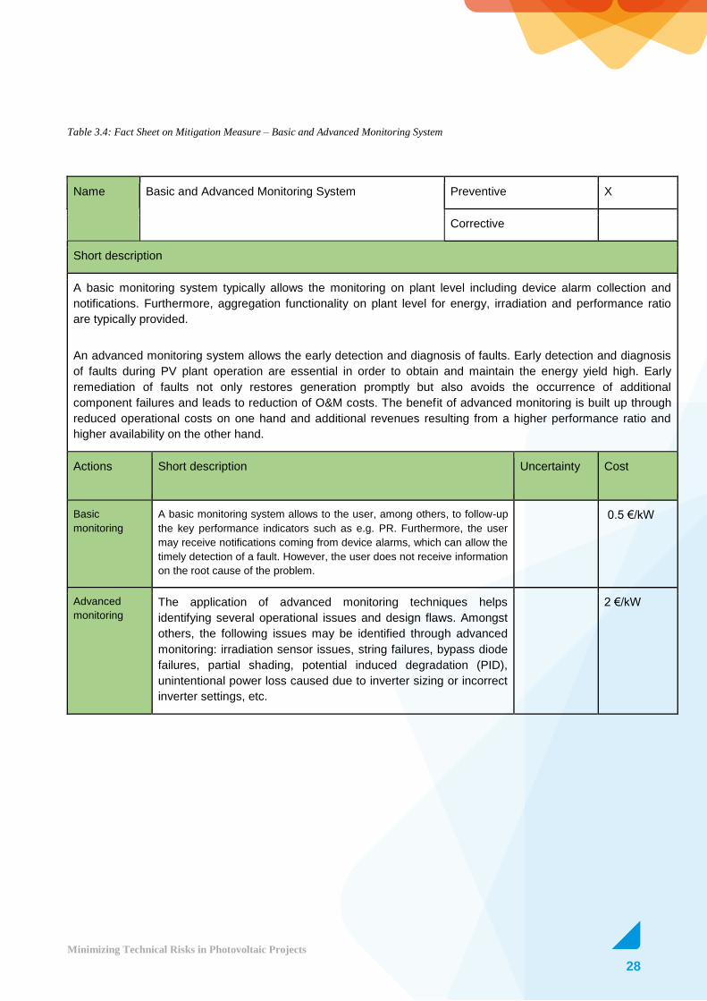
Table 3.4: Fact Sheet on Mitigation Measure – Basic and Advanced Monitoring System
Name Basic and Advanced Monitoring System Preventive X
Corrective
Short description
A basic monitoring system typically allows the monitoring on plant level including device alarm collection and
notifications. Furthermore, aggregation functionality on plant level for energy, irradiation and performance ratio
are typically provided.
An advanced monitoring system allows the early detection and diagnosis of faults. Early detection and diagnosis
of faults during PV plant operation are essential in order to obtain and maintain the energy yield high. Early
remediation of faults not only restores generation promptly but also avoids the occurrence of additional
component failures and leads to reduction of O&M costs. The benefit of advanced monitoring is built up through
reduced operational costs on one hand and additional revenues resulting from a higher performance ratio and
higher availability on the other hand.
Actions Short description Uncertainty Cost
Basic
monitoring
A basic monitoring system allows to the user, among others, to follow-up
the key performance indicators such as e.g. PR. Furthermore, the user
may receive notifications coming from device alarms, which can allow the
timely detection of a fault. However, the user does not receive information
on the root cause of the problem.
0.5 €/kW
Advanced
monitoring
The application of advanced monitoring techniques helps
identifying several operational issues and design flaws. Amongst
others, the following issues may be identified through advanced
monitoring: irradiation sensor issues, string failures, bypass diode
failures, partial shading, potential induced degradation (PID),
unintentional power loss caused due to inverter sizing or incorrect
inverter settings, etc.
2 €/kW
29
Minimizing Technical Risks in Photovoltaic Projects
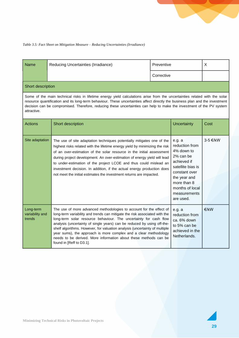
Table 3.5: Fact Sheet on Mitigation Measure – Reducing Uncertainties (Irradiance)
Name Reducing Uncertainties (Irradiance) Preventive X
Corrective
Short description
Some of the main technical risks in lifetime energy yield calculations arise from the uncertainties related with the solar
resource quantification and its long-term behaviour. These uncertainties affect directly the business plan and the investment
decision can be compromised. Therefore, reducing these uncertainties can help to make the investment of the PV system
attractive.
Actions Short description Uncertainty Cost
Site adaptation The use of site adaptation techniques potentially mitigates one of the
highest risks related with the lifetime energy yield by minimizing the risk
of an over-estimation of the solar resource in the initial assessment
during project development. An over-estimation of energy yield will lead
to under-estimation of the project LCOE and thus could mislead an
investment decision. In addition, if the actual energy production does
not meet the initial estimates the investment returns are impacted.
e.g. a
reduction from
4% down to
2% can be
achieved if
satellite bias is
constant over
the year and
more than 8
months of local
measurements
are used.
3-5 €/kW
Long-term
variability and
trends
The use of more advanced methodologies to account for the effect of
long-term variability and trends can mitigate the risk associated with the
long-term solar resource behaviour. The uncertainty for cash flow
analysis (uncertainty of single years) can be reduced by using off-the-
shelf algorithms. However, for valuation analysis (uncertainty of multiple
year sums), the approach is more complex and a clear methodology
needs to be derived. More information about these methods can be
found in [Reff to D3.1].
e.g. a
reduction from
ca. 6% down
to 5% can be
achieved in the
Netherlands.
€/kW

30
Minimizing Technical Risks in Photovoltaic Projects
4 Methodology
4.1 Definition of Best and Worst Uncertainty Scenarios
Some of the risks related to a PV project, already identified in (Moser et al., 2016) and included in
the risk matrix, have an economic impact in terms of uncertainty. In particular, the uncertainty can
be related either to the expected yield and performance indicators during the planning phase, or to
the actual yield and/or performance indicators during the operational phase. Figure 4.1 shows a list
of technical risks with impact on the uncertainty during the PV plant planning phase. It is interesting
to see that not all the components of a PV system are involved, and that also uncertainties related
to the assessment of the actual yield originate from phases preceding operation and maintenance.
In particular, this section focuses on defining several uncertainty scenarios of the input parameters
used for the design of a PV plant, with a focus on how these uncertainties propagate to the
expected yield and performance ratio. Therefore, it is first of all necessary to define a general
model that describes the relation between input parameters, and between input parameters and
output quantities. In Figure 4.2 a possible structure of such a model is shown. The PV array model
receives input from the temperature and irradiance models, and generates the expected array yield
by also taking several array losses into account. Finally, the yield is fed into the PV inverter model
in order to estimate the final yield of a PV system. In Figure 4.2, all risks that have an impact in
terms of uncertainty on the model are reported in different colours depending on the PV plant
component related to it. It is worth to note that some of the uncertainties associated to a risk can
have a direct impact on a model or sub-model, while others can also affect the uncertainty of other
risks. For example, an incorrect estimation of the power rating has a direct impact on the PV array
model (wrong nominal power inserted in the simulation software), but might also lead to an
incorrect sorting of the modules right before their installation, which in turn may cause losses in the
energy generation due to power mismatch of modules.

31
Minimizing Technical Risks in Photovoltaic Projects
Figure 4.1: List of the risks having an economic impact in terms of uncertainty of either estimated or actual yield of a PV plant.
Numbers are taken from the list of risks presented in (Moser et al., 2016)
The schematic model in Figure 4.2 is a general overview of the PV energy conversion chain and
the inter-relation of the different steps (input parameters and models) involved. Several software
tools implement irradiance, temperature, PV array and PV system models with different
characteristics (i.e. number and type of input parameters, type of sub-models used) and different
levels of complexity. In general, two methodologies are typically used to estimate the uncertainty
propagation: the Monte Carlo technique and the classical law of propagation of errors (“JCGM
100:2008(E),” 2008). The Monte Carlo approach allows reconstructing the Probability Density
Function (PDF) of the errors of a model starting from the information on the PDF of the errors of its
input quantities. This way, if a high (i.e. statistically significant) number of values of each input
parameter is generated according to the distribution of its error, and the corresponding number of
simulations is run, the resulting model outputs can be statistically analyzed in order to reconstruct
the PDF of their error and calculate their uncertainty. The Monte Carlo technique is particularly
useful and reliable when applied to models described by complex equations, in which also
correlations between input parameters may occur. In this case, the application of classical law of
propagation of errors might become a difficult task. In order to overcome this problem, some
approximations can be introduced. As reported by Thevenard et al (Thevenard and Pelland, 2011)
it is possible to represent a PV model with a good approximation as the product of linear factors:
output = input x proportionality factor – offset

32
Minimizing Technical Risks in Photovoltaic Projects
where the offset is relatively small compared to the phenomenon itself. If a quantity X is the
product of N independent variables X1, X2, ..., XN and can be expressed as X=c*X1*X2*...*XN, where
c is a constant and σ1, σ2, ..., σN are the uncertainties (corresponding to the standard deviations),
then the so-called rule of squares can be applied and the combined relative uncertainty of X
becomes:
𝜎𝑋
𝑋= √(
𝜎1
𝑋1)
2+ (
𝜎2
𝑋2)
2+ … + (
𝜎𝑁
𝑋𝑁)
2 (4.1)
Figure 4.2: General schematic of a model for the estimation of the yield of a PV system. Risks generating uncertainty are reported
with a representative value of associated uncertainty, and colored depending on the related component. Mutual influences are
indicated by arrows.
In order to compare the two methodologies, both are applied to estimate the uncertainty related to
the planning of a 4kWp PV system in Bolzano (South Tyrol, Italy). The main characteristics of the
PV plant and the input parameters involved in the calculations are presented in Table 4.1. The
information on the uncertainty of the input parameters, i.e. the distribution characteristics of their
errors is presented in Table 4.2, and refers to a base uncertainty scenario. These values have
been assigned on the basis of the information on the PV plant and on the site that is really
available, and in particular on a 20-year period of meteorological data (i.e. global horizontal
irradiance, diffuse horizontal irradiance, ambient temperature and wind speed) from satellite

33
Minimizing Technical Risks in Photovoltaic Projects
estimates. In order to apply the Monte Carlo technique, a number of 1000 values (N) was
generated for each considered input parameter, according to the PDF of their errors as reported in
Table 4.2. The software used for this exercise is Statistics101 (“Statistics101 - Grosberg,” 2016).
The selected number of draws is estimated sufficient to have statistical significance for this
exercise. In the next step, the 1000 generated values of each input parameter were combined in
1000 input vectors, and fed into the simulation software PVSyst (“PVSyst,” 2016). The software
therefore calculated 1000 values of global tilted irradiance (GTI), array yield (Ya), final yield (Yf)
and Performance Ratio (PR) for the considered PV plant.
Figure 4.3 shows the frequency distributions and the cumulative frequency distributions of the error
of Ya, Yr and PR that seem to resemble the normal distribution with a good approximation. By
calculating the standard deviation of the error distribution, we finally calculated the uncertainty of
these parameters as shown in Figure 4.4. In the same figure, also the uncertainty calculated with
the rule of squares is reported. It is interesting to see that the values of uncertainty of GTI, Ya and
Yf are similar for the two methodologies (though values generated with the rule of squares are
slightly lower than that calculated with Monte Carlo), thus confirming the validity of the assumption
made in order to apply the classical law of propagation of errors. An exception rises for PR, where
the uncertainty of 5.77% from the rule of squares is much higher than the 0.78% with the Monte
Carlo technique. A reasonable explanation for this comes from the expression of PR (“IEC 61724 :
Photovoltaic System Performance Monitoring - Guidelines for Measurement, Data Exchange and
Analysis,” 1998):
𝑃𝑅 =𝑌𝑓
𝑌𝑟 (4.2)
Since PR is a function of two highly correlated variables (Yf depends on Yr), here the assumption
previously made (PV yield model as a product of independent variables) is not valid anymore and
the rules of squares is not adequate.

34
Minimizing Technical Risks in Photovoltaic Projects
Table 4.1: Main characteristics and settings of the simulated PV system in Bolzano
Module type 210Wp (crystalline Si)
Nominal power 3.8 kWp
Number of modules 18 polycrystalline-silicon
N. modules x n. strings 9 x 2
Inverter type 4000 W nominal power
Tilt and orientation 30° tilt, 188° azimuth
Soiling losses 0.5%
Module quality loss 1%
Thermal factor 29 W/ (m2 K)
Meteo file 22 years of satellite data
Table 4.2: Parameters describing the frequency distribution of the errors of the input parameters used for the 1000 simulations with
PVSyst. Only the base uncertainty case scenario is reported.
Parameter Insolation variability
Temp. variability
Temp. effects (thermal factor Uc)
Soiling losses Nominal power
Shape normal (calculated)
normal (calculated)
normal (calculated)
normal (assumed)
normal (assumed)
Relative uncertainty (standard deviation)
3.31% GHI 2.24% DiffHi (k=1)
0.43% (k=1) 0.14% (k=1) 0.49% (k=1) 0.98% (k=1)

35
Minimizing Technical Risks in Photovoltaic Projects
Figure 4.3: Frequency distribution and cumulative frequency distribution of the parameters array yield (Ya), final yield (Yf) and
performance ratio (PR), generated from 1000 simulations with PVSyst using input parameters errors distributed according to Table
4.2. Red line represents the corresponding normal distribution with empirical mean (μ) and standard deviation (σ). Only the base
uncertainty scenario is represented.
Figure 4.4: Propagation of the uncertainty from the simulation software (PVSyst) input to the different output parameters, using the
Monte Carlo technique and the rule of square. Only the base uncertainty scenario is considered.

36
Minimizing Technical Risks in Photovoltaic Projects
Further scenarios – best and worst-case
When planning a PV system, the available information can be different from case to case affecting
also the value of the associated uncertainty. For example, when considering the solar resource
parameter, which accounts for the most quote of the energy yield uncertainty as shown e.g. in
(Caroline Tjengdrawira and Mauricio Richter, 2016), the planner could have:
- Different time series ranges, i.e. different insolation variability: e.g., 1, 5, 20 etc. years of
available data
- Different insolation resources: e.g. measured, satellite-retrieved, or a combination of long-
term satellite data and short-term series of measured data (Achim Woyte et al., 2016;
Gueymard and Wilcox, 2009; Polo et al., 2016)
- Datasets of irradiance on the plane of array, or the need to use plane-of-array transposition
models from global and diffuse horizontal irradiance.
Further information is needed to define the value and the uncertainty of, among the most
important, the ambient temperature variability, the temperature coefficients or temperature effects,
the performance loss rate, the soiling losses, the shading losses, the spectral mismatch
gain/losses, the module nominal power and the inverter efficiency.
In order to analyse the variability of the uncertainty of the outputs of a generic PV model, several
uncertainty scenarios have been defined. These scenarios differ from the base uncertainty
scenario previously introduced:
- case 1: base uncertainty scenario (22 years of satellite-derived GHI and DiffHI in
Bolzano)
- case 2: 5 years of measured GHI and DiffHI in Bolzano
- case 3: 20 years of measured GHI and DiffHI in Bolzano
- case 4: combination of long-term satellite-derived GHI and DiffHI and short-term (1 year)
series of measured GHI and DiffHI
- case 5: 5 years of satellite-derived GHI and DiffHI in Bolzano
- case 6: 20 years of measured GHI and DiffHI in a site with high insolation variability
- case 7: 20 years of satellite-derived global tilted irradiance (GTI) in Bolzano
- case 8: 5 years of measured GTI in Bolzano
- case 9: 20 years of measured GTI in Bolzano
- case 10: combination of long-term satellite-derived GTI and short-term (1 year) series of
measured GTI
- case 11: 5 years of satellite-derived GTI in Bolzano
- case 12: 20 years of measured GTI in a site with high insolation variability
- case 13: worst transposition model for Bolzano
- case 14: high uncertainty of temperature effects (e.g. choice of temperature model not
accounting for wind effect)
- case 15: high variability of ambient temperature
- case 16: high uncertainty of performance loss rate

37
Minimizing Technical Risks in Photovoltaic Projects
- case 17: high uncertainty of shading effect (e.g. mountainous region, no measurement of
the horizon)
- case 18: high uncertainty of soiling effect (e.g. desert area, no estimation of soiling in the
region)
- case 19: high uncertainty of spectral mismatch effect (e.g. use of technology with narrow
spectral responsivity such as amorphous silicon)
- case 20: high uncertainty of nominal power
- case 21: high uncertainty of inverter efficiency
- case 22: worst-case (highest uncertainty for each input parameter).
The additional cases (2 to 22) have the same set of uncertainties of the base scenario, except for
the uncertainty of one single parameter (e.g. insolation variability, or solar resource, etc.), which
can be either higher or lower.
A complete list of all considered uncertainty scenarios, reporting the values of uncertainty
associated to each input parameter and the uncertainty of the PV model outputs calculated with
the rule of squares, is found in Appendix 5. Table 4.3 contains an overview of the uncertainties
used for each input parameter in the base and additional uncertainty scenarios, with a short
explanation regarding the choice of the values. It is worth to notice that all the uncertainty values of
Table 4.3 refer to the uncertainty on the energy yield. For example, the uncertainty on energy yield
due to soiling effect is 0.49%, which is calculated considering an average value of Ya of
4.13 kWh/kWp/day (calculated with PVSyst), a value of soiling loss of 0.5% (see Table 4.1) and an
uncertainty of 2% on this value.
A ranking list of the considered cases, based on the value of the uncertainty calculated on the final
yield of the 4 kWp PV plant in Bolzano with the rule of squares is reported in Table 4.4. The value
of uncertainty reported for the base uncertainty scenario does not correspond to that reported in
Figure 4.4, because the uncertainty propagation of more input parameters is involved in the
calculation. The results of Figure 4.4 refer to the propagation of a limited number of uncertainties
types, reflecting the limited number of input parameters that can be modified in the batch mode of
PVSyst. This issue will be further discussed in Section 4.3. In general, the following considerations
can be made:

38
Minimizing Technical Risks in Photovoltaic Projects
There is a group of cases assuring a low level of uncertainty (4.55% to 8.70%). This includes the
base case and the alternative cases with lower uncertainties than the base case. They all refer to
the use of long time-series of either ground measurements or satellite estimates of insolation.
The temporal range of the available insolation data seem therefore to be the most important factor
affecting the uncertainty of the yield estimation. There is for example a 5% improvement when
using 20 years instead of 5 years of GTI data, which increases up to 7.6% when GHI and DiffHI
data are used.
The best case corresponds to the use of 20 years of measured values of GTI, showing also
that a lower uncertainty is assured when a) ground measurements are used in place of satellite
estimates and b) time series of plane-of-array irradiance is available without the need to
apply transposition models. In the first case there is, for example, a 1.9% improvement when
using long series of measured GTI data, which increases up to 2.9% when using long series of
measured GHI and DiffHI data. Results show also that using a combination of long time series of
satellite data with a short series of measured data is recommended than just using satellite data.
In the case a PV plant is to be installed in a location with high insolation variability, the uncertainty
of the yield estimation is also negatively affected. For example, if the same considerations made
for Bolzano were applied for London, at least an additional 3% should be added in the final yield
uncertainty.
Besides the insolation variability and the solar resource quantification uncertainty, the
uncertainties related to shading and soiling effects and to the use of transposition models
play also a role in the overall uncertainty of the final yield.
In general, the uncertainty of the final yield of the 4kWp plant installed in Bolzano ranges from
4.5% to 14.9%. The latter becomes a 16.6% in the eventuality that the planner has the worst
information quality available.

39
Minimizing Technical Risks in Photovoltaic Projects
Table 4.3: List of uncertainties assumed for the different input parameters, both in the base uncertainty scenario and in the
alternative uncertainty scenarios
Scenario Description Rel. unc. (st.dev,
k=1) Note
Insolation variability
Base 20 years of data 3.31% calculated from the weather files. Same value for GHI, DiffHI, GTI
Alternative 5 years of data 9.00% Same value for GHI, DiffHI, GTI
Alternative 20 years of data, high
variability due to location 7.10% Same value for GHI, DiffHI, GTI
Solar resource
Base satellite estimates 5.00% from Suri et al. (Suri et al., 2007) and Richter et al. (Richter, M et
al., 2015)
Alternative ground measurements 2.00% supposing to use a secondary
standard pyranometer
Alternative
combination of long-term satellite data and short-term series of measured data [ref
3E]
3.00% from Gueymard et al. (Gueymard
and Wilcox, 2009)
Transposition model Base good transposition model 2.00%
proven to be good for the specific location
Alternative bad transposition model 5.40% (Cameron et al., 2008)
Ambient temperature variability
Base 20 years of data 0.43% calculated from the weather files
Alternative highest reported by SB
deliverable 2.00%
highest value (Moser et al., 2016) [Technical Risks in PV Projects,
page 50]
Temperature effect
Base best temperature model 0.14%
using a temperature model that accounts for wind effect (e.g.
Koehl (Koehl et al., 2011)), proven to be good for the considered location (Schwingshackl et al.,
2013)
Alternative worst temperature model 1.15%
using a temperature model that does not account for wind effect
(e.g. NOCT formula), proven to be bad for the considered location
Performance loss rate
Base low uncertainty 0.50%
Alternative high uncertainty 2.00% highest value (Moser et al., 2016) [Technical Risks in PV Projects,
page 50]
Soiling effect Base low uncertainty 0.49%
calculated from 2% uncertainty of soiling losses
Alternative high uncertainty 4.00% highest value according to Reich et al., 2015 (Reich et al., 2015)
Shading effect Base low uncertainty 2.00%
Alternative high uncertainty 5.00%
Spectral mismatch effect
Base low uncertainty 0.20%
Alternative high uncertainty 2.00%
Nominal power of the modules
Base low uncertainty 0.98%
Alternative high uncertainty 2.00% highest value (Moser et al., 2016) [Technical Risks in PV Projects,
page 50]
Inverter efficiency effect
Base low uncertainty 0.20%
Alternative high uncertainty 0.50% highest value (Moser et al., 2016) [Technical Risks in PV Projects,
page 50]

40
Minimizing Technical Risks in Photovoltaic Projects
Table 4.4: Ranking list of the base and alternative uncertainty scenarios based on the calculated value of uncertainty on the final
yield of the 4 kWp PV system installed in Bolzano
Relative Uncertainty on Yf
Case Number
Description
4.55% 9 20 years of measured GTI in Bolzano
5.07% 10 combination of long-term satellite-derived GTI and
short-term (1 year) series of measured GTI
5.80% 3 20 years of measured GHI and DiffHI in Bolzano
6.45% 7 20 years of satellite-derived GTI in Bolzano
6.61% 4 combination of long-term satellite-derived GHI and
DiffHI and short-term (1 year) series of measured GHI and DiffHI
7.76% 12 20 years of measured GTI in a site with high insolation
variability
8.70% 1 base uncertainty scenario (20 years of satellite GHI
and DiffHI in Bolzano)
8.71% 21 high uncertainty of inverter efficiency
8.77% 14 high uncertainty of temperature effects (e.g. choice of
temperature model not accounting for wind effect)
8.87% 20 high uncertainty of nominal power
8.91% 16 high uncertainty of performance loss rate
8.92% 15 high variability of ambient temperature
8.92% 19 high uncertainty of spectral mismatch effect (e.g. use of technology with narrow spectral responsivity like
amorphous silicon)
9.53% 8 5 years of measured GTI in Bolzano
9.56% 18 high uncertainty of soiling effect (e.g. desert area, no
estimation of soiling in the region)
9.83% 17 high uncertainty of shading effect (e.g. mountainous
region, no measurement of the horizon)
10.04% 13 worst transposition model for Bolzano
10.57% 11 5 years of satellite GTI in Bolzano
10.89% 6 20 years of measured GHI and DiffHI in a site with
high insolation variability
13.41% 2 5 years of measured GHI and DiffHI in Bolzano
14.89% 5 5 years of satellite-derived GHI and DiffHI in Bolzano
16.58% 22 worst-case (highest uncertainty for each input
parameter)
41
Minimizing Technical Risks in Photovoltaic Projects
4.2 CPN Reduction by Different Mitigation Measures
Besides the technical risks associated with uncertainties during project planning phase, the second
group of risks has a direct economic impact during operation. These risks were already identified
and evaluated in “Report Technical Risks in PV Projects” (Moser et al., 2016). The methodology of
quantification was also introduced in chapter 5 of the mentioned report.
The developed method is now applied on the evaluation of the effectiveness of the identified
mitigation measures. To this extent, Risk Mitigation Factors (RMF) are introduced which quantify
the reduction of costs for fixing the failures (i.e. repair of existing component, substitution by spare
component, substitution by new component). Therefore, three new parameters are defined as risk
mitigation factors. Depending on the category of mitigation, the impact is:
(α) mitigation of number of failures
(β) mitigation of time to detection
(γ) mitigation of time to repair.
The quantitative impact is given by a number between 0 - 1. If a mitigation measure has no impact
on a certain failure, the related risk reduction factor is 1. If the risk parameter is completely
eliminated after the mitigation, the risk mitigation factor becomes 0. This means that with α of 0.5
the number of failures can be reduced to 50% and with β of 0.5 the time to detection can be
reduced to 50% of the time without mitigation.
Thus, the mitigated number of failures is calculated as follows:
𝑛𝑓𝑎𝑖𝑙,𝑚𝑖𝑡 = 𝛼 ⋅ 𝑛𝑓𝑎𝑖𝑙
The mitigated time to detection is calculated as follows:
𝑡𝑡𝑑,𝑚𝑖𝑡 = 𝛽 ⋅ 𝑡𝑡𝑑
and the mitigated time to repair/substitution is calculated as follows:

42
Minimizing Technical Risks in Photovoltaic Projects
𝑡𝑡𝑟/𝑡𝑠,𝑚𝑖𝑡 = 𝛾 ⋅ 𝑡𝑡𝑟/𝑡𝑠
When several mitigation measures with impact on the same risk mitigation factor are considered,
the individual risk mitigation factors are multiplied with each other and the risk is further reduced.
The risk mitigation factor α, respectively β and γ, is then calculated as follows:
𝛼 = 𝛼1 ⋅ 𝛼2 ⋅ 𝛼3 . . . = ∏
𝑛
𝑖=1
𝛼𝑖
Implementing the new mitigation factors into the CPN model leads to the following mitigated
downtime costs (€):
𝐶𝑑𝑜𝑤𝑛,𝑚𝑖𝑡 = 𝐶𝑑𝑜𝑤𝑛,𝑡𝑑,𝑚𝑖𝑡 + 𝐶𝑑𝑜𝑤𝑛,𝑡𝑟/𝑡𝑠,𝑚𝑖𝑡 + 𝐶𝑑𝑜𝑤𝑛,𝑓𝑖𝑥,𝑚𝑖𝑡
- mitigated downtime costs to detection:
𝐶𝑑𝑜𝑤𝑛,𝑡𝑑,𝑚𝑖𝑡 = 𝛼 ⋅ 𝑛𝑓𝑎𝑖𝑙/𝑛𝑐𝑜𝑚𝑝 ⋅ 𝛽 ⋅ 𝑡𝑡𝑑/𝑡𝑟𝑒𝑓 ⋅ 𝑃𝐿 ⋅ 𝑀 ⋅ 𝑃𝑃𝐴 ⋅ 𝑌 = 𝛼 ⋅ 𝛽 ⋅ 𝐶𝑑𝑜𝑤𝑛,𝑡𝑑
- mitigated downtime costs to repair/substitution:
𝐶𝑑𝑜𝑤𝑛,𝑡𝑟/𝑡𝑠,𝑚𝑖𝑡 = 𝛼 ⋅ 𝑛𝑓𝑎𝑖𝑙/𝑛𝑐𝑜𝑚𝑝 ⋅ 𝛾 ⋅ 𝑡𝑡𝑟/𝑡𝑠/𝑡𝑟𝑒𝑓 ⋅ 𝑃𝐿 ⋅ 𝑀 ⋅ 𝑃𝑃𝐴 ⋅ 𝑌 = 𝛼 ⋅ 𝛾 ⋅ 𝐶𝑑𝑜𝑤𝑛,𝑡𝑟/𝑡𝑠
and mitigated downtime costs during repair/substitution:
𝐶𝑑𝑜𝑤𝑛,𝑓𝑖𝑥,𝑚𝑖𝑡 = 𝛼 ⋅ 𝑛𝑓𝑎𝑖𝑙/𝑛𝑐𝑜𝑚𝑝 ⋅ 𝑡𝑓𝑖𝑥/𝑡𝑟𝑒𝑓 ⋅ 𝑀 ⋅ 𝑃𝑃𝐴 ⋅ 𝑌 = 𝛼 ⋅ 𝐶𝑑𝑜𝑤𝑛,𝑓𝑖𝑥

43
Minimizing Technical Risks in Photovoltaic Projects
In addition to downtime costs, the costs for fixing the failures is the second main parameter. It
considers the costs of repair and substitution of parts (𝐶𝑟𝑒𝑝/𝑠𝑢𝑏), costs of transportation (𝐶𝑡𝑟𝑎𝑛𝑠),
labour costs (𝐶𝑙𝑎𝑏) and also the costs of detection and mitigation depending on the applied
mitigation measures (𝐶𝑑𝑒𝑡/𝑚𝑖𝑡). It is calculated as follows:
𝐶𝑓𝑖𝑥,𝑚𝑖𝑡 = 𝛼 ⋅ 𝑛𝑓𝑎𝑖𝑙 ⋅ [𝐶𝑑𝑒𝑡/𝑚𝑖𝑡 + 𝐶𝑟𝑒𝑝/𝑠𝑢𝑏 + 𝐶𝑡𝑟𝑎𝑛𝑠 + (𝐶𝑙𝑎𝑏 ∗ 𝑡𝑓𝑖𝑥)] = 𝛼 ⋅ 𝐶𝑓𝑖𝑥
The calculation of the mitigated CPN is then given by:
𝐶𝑃𝑁𝑚𝑖𝑡 = 𝐶𝑑𝑜𝑤𝑛,𝑚𝑖𝑡 + 𝐶𝑓𝑖𝑥,𝑚𝑖𝑡.
4.3 Critical Aspects of the Proposed Approaches
4.3.1 Error Propagation in Yield Uncertainty for Failures during Planning
In Section 4.1 the Monte Carlo technique has been used to calculate the propagation of uncertainty
of the input parameters of a PV simulation software or model to its outputs (generated energy,
performance indexes etc.). This methodology is preferable when the model to which it is applied is
made up of non-linear and not differentiable equations, as prescribed by GUM (“BIPM - Guide to
the Expression of Uncertainty in Measurement (GUM),” n.d.) . In this case, the Monte Carlo is
expected to be more rigorous and correct than the classical rule of squares. As demonstrated in
Section 4.1, the application of the two methodologies to the estimation of the energy yield of a PV
plant generates similar results, with the exception of the Performance Ratio index. Therefore, in
this case the use of the Monte Carlo technique would be preferable to the rule of sum of squares.
However, some critical aspects can be highlighted in the application of this methodology. First of
all, Monte Carlo is a statistical technique that requires a high number of simulations in order to
assure that the results have statistical significance. Therefore, a significant level of computational
resources must be guaranteed. Another aspect concerns the current available software for the
calculation of the of energy productivity of a PV plant. An ideal software should allow the user a) to
set a sufficient number of input parameters needed to perform a reliable uncertainty propagation
analysis; and b) to give the possibility to run simulations in batch mode, i.e. to execute scripts.
Unfortunately, to the authors’ knowledge, the implementation of both features has not been done
yet in any of the available commercial software, or only partially.

44
Minimizing Technical Risks in Photovoltaic Projects
4.3.2 CPN methodology and mitigation measures
Mitigation measures as described in the methodology have an impact limited to the number of
failures, time to detection, and time to repair/substitution through the Risk Mitigation Factors. Some
specific mitigation measures could have an impact also on other parameters included in the CPN
methodology but not fully exploited in this report. For example, the availability of spare parts could
also have an impact on the cost of repair and substitution: when the failure occurs, a specific
product might not be available on the market anymore (e.g. module from a specific manufacturer or
with a certain nominal power) or available only at higher costs.
Other issue is represented by the complexity of carrying out a comprehensive analysis of the effect
of combined mitigation measures. In this report, mitigation measures have been grouped with a
broad scoped. The impact of specific mitigation measures such as video surveillance, effective
insurance cover, predictive monitoring, just to name a few, are to some extent included in the
analysis but each individual contribution is not specified. This was the results of a trade-off
between the need to analyse various mitigation measures and the complexity of the analysis.
It has to be stressed that the methodology already allows or can be easily modified to include the
aforementioned analysis.
5 Analysis and Results
5.1 Impact on Initial Energy Yield Prediction and Exceedance
Probability for the Defined Scenarios with Reduced
Uncertainties
As also covered in the report “Review and Gap Analyses of Technical Assumptions in PV
Electricity Cost” (see chapter 3.1.2) (Tjengdrawira and Richter, 2016), a common way to quantify
the technical risks arising during the PV planning phase, is to calculate the exceedance probability
as, e.g., P50/P90. Typically, for the various elements concurring to the final uncertainty of the
energy yield, a normal distribution is assumed. In section 4.1 of this report, instead of relying on a
normal distribution, we have opted for an empirical method based on a Monte Carlo analysis. The
result is an empirical cumulative distribution function from which the exceedance probabilities can
be interpolated.
The use of empirical methods can thus be regarded as the most advanced mitigation measure in
reducing the risks in the initial yield assessment as it allows the inclusion of data which might not
be normally distributed.

45
Minimizing Technical Risks in Photovoltaic Projects
Figure 5.1 shows the comparison between the results of the Monte Carlo analysis and a normal
distribution with a mean (μ) specific energy yield value of 1445 kWh/kWp and standard deviation
(σ) of 4.6% (k=1) as taken from Chapter 4.1.
Figure 5.1: Comparison of the cumulative distribution function for a normal distribution with σ=4.6% (k=1) (black curve) and the
results from a Monte Carlo analysis (red curve)
It is by coincidence that the P90/P50 ratio is very similar for both distributions (94.4%). What differs
are the absolute values of P50 and P90 (-0.35% for the empirical distribution). The empirical
distribution is positively skewed and shows important differences for values <P50 (e.g. -6.6% at
P10 for the empirical distribution). In addition, extreme scenarios (e.g. P99) can largely be affected
by the use of normal distribution yielding unrealistic results. Similar results were obtained for the
analysis of the long-term solar resource as presented in deliverable D3.1 of the Solar Bankability
project (Tjengdrawira and Richter, 2016), where it is shown that assuming a normal distribution for
the solar resource uncertainties may not be the most correct approach.
Unfortunately, there is not always a sufficiently large dataset available to establish the CDF from
which to interpolate exceedance probabilities. Nevertheless, for some elements involved in the
calculation of the long-term expected yield as, e.g. the solar resource, this method can be applied.
With the availability of more data for other elements, also other secondary effects can be included
in the methodology as not normally distributed.

46
Minimizing Technical Risks in Photovoltaic Projects
Figure 5.2: Comparison of the three scenarios assuming a normal distribution
The possibility of running a full-scale Monte Carlo analysis requires knowledge on the distribution
of each element contributing to the overall uncertainty of the energy yield. If we restrict the analysis
on normally distributed energy yield, we can look at the effect of the results obtained in section 4.1
for the various cases (see also Annex 5). For the 22 cases, the uncertainty varies between 4.6%
(here defined as the low-end scenario) and 16.6% (here defined as the worst-case scenario). A
high-end scenario was defined as the average without the outliers resulting in a σ=9.3%. The low
end and high end scenarios are thus representative for the range given in (Moser et al., 2016) of 5-
10% overall uncertainty of the energy yield. Here the impact of the uncertainty on the CDF is
evident and the resulting P50, P90 and P90/P50 values are summarised in Table 5.1 and shown in
Figure 5.2. The P90 values decrease respectively by -6% and -15% when compared to the low-end
scenario.

47
Minimizing Technical Risks in Photovoltaic Projects
Figure 5.3: Comparison of the worst case scenario with different mean values of the normal distribution with σ=16.6%
Another important parameter which affects the overall analysis is the mean value of the energy
yield (P50 if normally distributed). The main source of error is related to the solar resource
assessment. Figure 5.2 shows the results for the worst-case scenario with a mean value of
1314 kWh/kWp instead of 1445 kWh/kWp. These values come from a solar resources assessment
based on 5-year-measured data and 20-year-satellite-derived data, respectively. The use of
shorter time series can clearly lead to an underestimation (or overestimation) of the mean value
depending if the tails of the distribution are present or not. When compared to the low-end
scenario, the reduction in P90 for this specific case is 22%.
Table 5.1: Summary of the exceedance probability values for various scenarios
σ (k=1) P50 (kWh/kWp) P90 (kWh/kWp) P50/P90 (P50
reference case)
Reference case (PVSYST, not all contributions included)
4.3% 1440 1360 94%
Ref. case (sum of squares)
8.7% 1445 1283 89%
Low end scenario 4.6% 1445 1365 94%
High end scenario 9.3% 1445 1273 88%
Worst case scenario 16.6% 1445 1138 79%
Worst case scenario (different mean value) 16.6% 1314 1034 72%

48
Minimizing Technical Risks in Photovoltaic Projects
To deepen the analysis and understand how initial yield assessments relates with actual data
during operation, the Solar Bankability project compared the initial long-term yield estimates
against the actual production over a portfolio of 41 PV plants. This analysis is presented in
(Caroline Tjengdrawira and Mauricio Richter, 2016). Results show that the dispersion (nRMSE)
across the portfolio between initial yield estimates and actual production over the first years is
around 4.4%. This lies towards the low-end scenario as presented in this analysis. However, for
some extreme cases within the portfolio the difference is around 8 to 10%, lying more towards the
reference case and high-end scenario.
Once the CDF of the yield is assessed for a specific plant or for a portfolio of PV plants, the
exceedance probability values of the yield can be used as input for the parameter “Severity” as
included in the CPN methodology (defined as the yield of a PV plant or a portfolio of PV plants
unaffected by failures during operation). This would lead to a calculation of the distribution of CPNs
with the possibility of assessing the risk related also to Cost Priority Numbers in terms of CPN50
and CPN90.
The methodology presented in 4.1 and the results shown in this section can then be directly linked
to the CPN methodology to provide an overall framework for the analysis of the economic impact of
technical risks.
5.2 Impact of Applied Mitigation Measures on and Ranking of CPN
The economic impact of various mitigation measures are here reviewed and quantitatively
evaluated based on the described methodology. In addition, the measures with the highest cost to
benefit ratio are identified in order to facilitate the selection of suitable measures and their
combinations.
The following eight of the already introduced mitigation measures are assessed. The pre-selection
was made after research of the most common measures as defined in the gap analysis presented
by (Tjengdrawira and Richter, 2016) and a representation of measures influencing the three
parameters described nfail, ttd and ttr / ts.

49
Minimizing Technical Risks in Photovoltaic Projects
Table 5.2: List of most significant measures, their mitigation factors and affected parameters
Mitigation Measure Risk Mitigation Factor Affected Parameter
Component testing – PV modules
α number of failures
Design review + construction monitoring
α number of failures
Qualification of EPC α number of failures
Advanced monitoring system β time to detection
Basic monitoring system β time to detection
Advanced inspection β time to detection
Visual inspection β time to detection
Spare part management γ time to repair/substitution
The implementation of the measures is performed based on a reference scenario, limited to the
utility scale segment of the database described in (Moser et al., 2016). The downtime is based on
the “never detected” scenario without mitigation measures (the never detected scenario was
defined with a 12 months lead-time to detection), here referred as LOSS scenario. The FIX
scenario instead is dedicated to the cost of fixing the failure.
The total CPN is calculated from the sum of the individual CPN of all failures. The new CPN is the
sum of the mitigated CPN including the costs incurred for the mitigation measures. The benefit of
the combination of the measures resulting from the difference between total CPN and new CPN is
then given by:
𝐶𝑃𝑁𝑛𝑒𝑤 = 𝐶𝑃𝑁𝑚𝑖𝑡 + 𝐶𝑜𝑠𝑡𝑚𝑖𝑡
The applied costs of the mitigation measures are defined in Table 5.3 where three different cost
scenarios are introduced: medium cost scenario (1), low cost scenario (2) and high cost
scenario (3). They mark the lower and upper range of the applied costs for the new CPN
calculations.
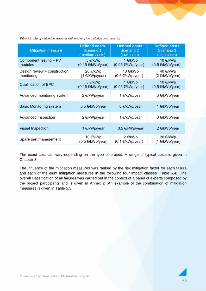
50
Minimizing Technical Risks in Photovoltaic Projects
Table 5.3: List of mitigation measures with medium, low and high cost scenarios
Mitigation measure Defined costs
Scenario 1 (medium costs)
Defined costs Scenario 2 (low costs)
Defined costs Scenario 3 (high costs)
Component testing – PV modules
3 €/kWp (0.15 €/kWp/year)
1 €/kWp (0.05 €/kWp/year)
10 €/kWp (0.5 €/kWp/year)
Design review + construction monitoring
20 €/kWp (1 €/kWp/year)
10 €/kWp (0.5 €/kWp/year)
40 €/kWp (2 €/kWp/year)
Qualification of EPC 3 €/kWp
(0.15 €/kWp/year) 1 €/kWp
(0.05 €/kWp/year) 10 €/kWp
(0.5 €/kWp/year)
Advanced monitoring system 2 €/kWp/year 1 €/kWp/year 3 €/kWp/year
Basic Monitoring system 0.5 €/kWp/year 0 €/kWp/year 1 €/kWp/year
Advanced Inspection 2 €/kWp/year 1 €/kWp/year 3 €/kWp/year
Visual Inspection 1 €/kWp/year 0.5 €/kWp/year 2 €/kWp/year
Spare part management 10 €/kWp
(0.5 €/kWp/year) 2 €/kWp
(0.1 €/kWp/year) 20 €/kWp
(1 €/kWp/year)
The exact cost can vary depending on the type of project. A range of typical costs is given in
Chapter 3.
The influence of the mitigation measures was ranked by the risk mitigation factor for each failure
and each of the eight mitigation measures in the following four impact classes (Table 5.4). The
overall classification of all failures was carried out in the context of a panel of experts composed by
the project participants and is given in Annex 2 (An example of the combination of mitigation
measures is given in Table 5.5.

51
Minimizing Technical Risks in Photovoltaic Projects
Table 5.4: Definition of impact classes with respect to risk mitigation factor (RMF)
Impact Classes RMF (α,β,γ)
High 99.5 %
Medium 50.0 %
Low 25.0 %
No 0.0 %
Table 5.5: Example of combination of mitigation measures
Figure 5.4: Top 10 risks of PV modules with and without mitigation measures in CPN

52
Minimizing Technical Risks in Photovoltaic Projects
Figure 5.5. Top 10 risks of inverter with and without mitigation measures in CPN
Figures 5.4 and 5.5 show two examples of risk mitigation benefits in terms of CPN for the top 10
risks of PV modules and inverters. For these two examples the cost of the mitigation measure was
spread over each specific failure. The CPN without any mitigation measures (blue bars) is
compared to the CPN resulting from the best combination of mitigation measures (red bars) for
each of the top 10 failures. When the CPN related to the mitigation measures is nearly zero, the
benefit is the highest. This is the case for risks, which can easily be reduced by preventive
measures e.g. bad installation, PID and defective back sheet for module risks (see Fig. 5.4) and
wrong installation and grounding faults for inverter risks (see Fig. 5.5).
A right combination of mitigation measures can be very effective taking a failure specific CPN down
to nearly zero.
5.2.1 Mitigation measures applied to the FIX scenario
The costs related to FIXING the failures result from the sum of the costs of repair/substitution, the
costs of detection, the costs of transportation, and the cost of labour. Figure 5.6 shows the results
of calculating the FIXING costs for selected failures when applying the eight mitigation measures
listed in Table 5.3. The selection of failures was based on experts’ panels and include the top 20
PV module failures, top 20 inverter failures, failures of mounting structure, combiner boxes, cabling
as well as failures of transformer station as listed in Annex 2 of this report.
The total CPN without mitigation measures is 104.75 €/ kWp/year for the defined FIX scenarios,
defined as FIX Reference. The CPNnew for all 256 combinations of mitigation measures are shown
in Fig. 5.6 below. The total CPN without mitigation measures is given by the green area at
104.75 €/kWp/year. Applying specific mitigation measures (e.g. combinations 192 – 255 as given
in Annex 3) it is possible to significantly reduce the risks and to obtain values of CPNnew in the
order of 15 to 20 €/kWp/year (see Fig. 5.6). The index of combinations can be found in Annex 3.

53
Minimizing Technical Risks in Photovoltaic Projects
Figure 5.6: New CPN results of mitigation measure combinations for different FIX cost scenarios compared to CPN without MM –
Index of mitigation measure combinations is given in Annex 3.
Table 5.6: Best combinations of mitigation measures for medium (1), low (2) and high (3) cost scenarios and their savings in CPN
(last column)

54
Minimizing Technical Risks in Photovoltaic Projects
Table 5.6 shows the corresponding savings of those mitigation measures for the best combinations
(Rank 1 to 10) and for the three cost scenarios. The savings ranging between 85 and
91 €/kWp/year are given by the difference between the total CPN (104.75 €/kWp/year) and the
new CPN. The savings for low cost scenario (2) are slightly higher than for the medium (1) and
high cost (3) scenario (see Tab. 5.6).
The following outcome can be derived from the results shown in Fig. 5.6 and Table 5.6:
For all 256 combinations of mitigation measures the CPNnew for FIXING low cost scenario 2
shows better results than for FIX medium 1 and for FIX high cost scenarios 3 as expected.
Preventive measures have the highest impact on CPNnew e.g. Qualification of EPC (index of
mitigation measure combination 32 to 63) will bring down CPNnew to 75 €/kWp/year. E.g.
Design review (index of combination 64 to 95) will further reduce CPNnew to 40 €/kWp/year
(see Fig. 5.6).
Corrective measures have less impact on CPNnew e.g. Basic and advanced monitoring and
visual and advanced inspection (index of combination 1 to 31 – Fig. 5.6). However,
corrective measures can be very important, when it comes to assigning liabilities at the end
of the guarantee or warrantee period.
Reducing the number of failures has the highest impact due to the high substitution costs.
The highest savings for all three cost scenarios can be achieved by applying the three
preventive measures (component testing plus design review plus qualification of EPC) as
shown in the first three columns of Table 5.6. The savings may reach 90 €/kWp/year for the
best combinations of selected mitigation measures.
As shown in Fig. 5.6, for 99% of all mitigation measure combinations the scenarios will
result in economic benefit by reducing the CPNnew to values lower than 104.75€/kWp/year.
5.2.2 Mitigation measures applied to the LOSS scenario
The LOSS scenario is focused on the economic losses due to downtime. Figure 5.7 and Figure 5.8
show the results of calculating the LOSS costs for the same failures as in Fig. 5.6 (Annex 2) when
applying the eight mitigation measures listed in Table 5.3. For the calculation of the LOSS costs
due to downtime, it is important to consider the missing income of feed-in tariffs or the missing
income from Power Purchasing Agreement (PPA) or the missing savings in terms of Retail Cost of
Electricity for PV plants on roofs. Here, we consider high PPA (0.25€/kWh) and low PPA
(0.10€/kWh) for the three different cost LOSS scenarios of large-scale PV plants.
The total CPN without mitigation measures is 13.5 €/kWp/year for the defined LOSS scenarios,
also known as “never detected”, defined as LOSS Reference based on high PPA value
(0.25€/kWh). The CPNnew values for all 256 combinations of mitigation measures are shown in
Fig. 5.7 below. The total CPN without mitigation measures is given by the green area at
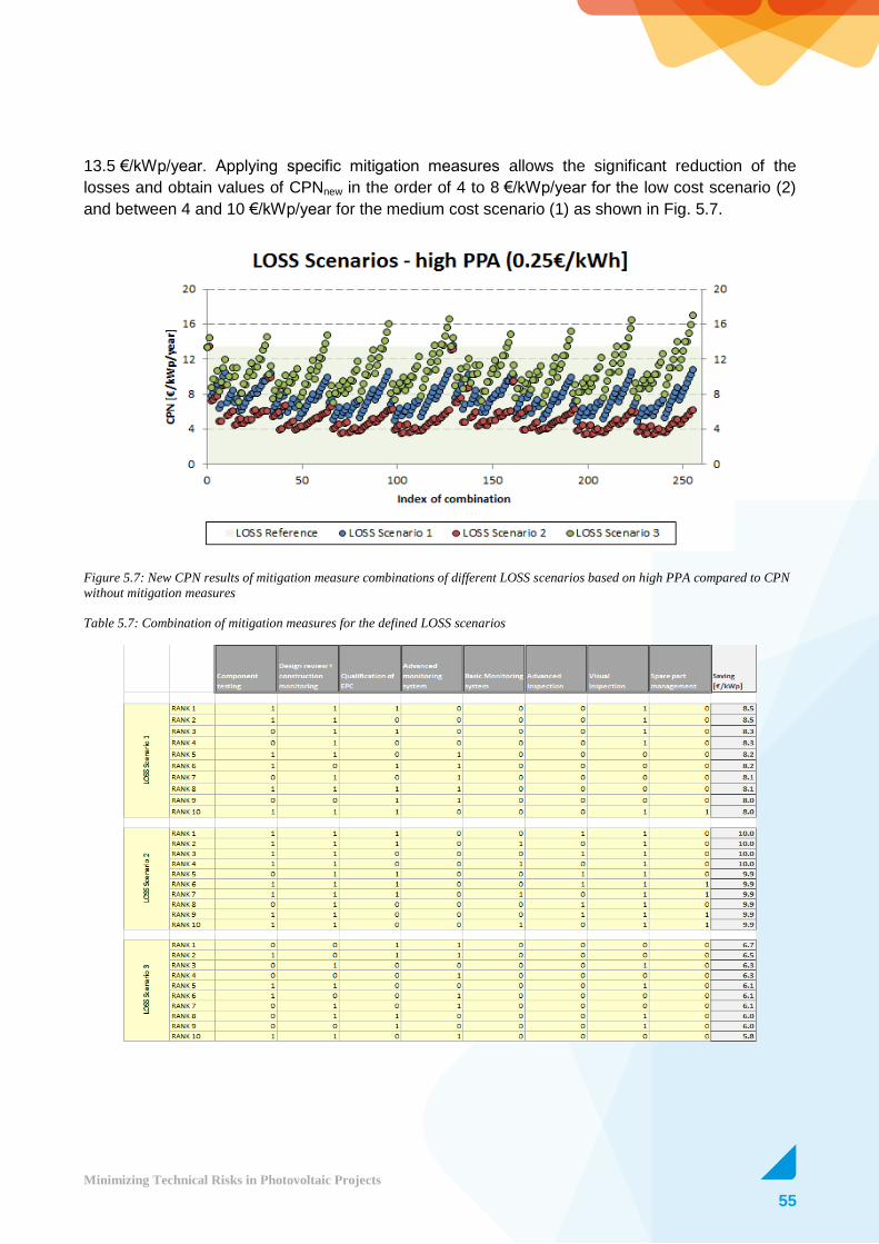
55
Minimizing Technical Risks in Photovoltaic Projects
13.5 €/kWp/year. Applying specific mitigation measures allows the significant reduction of the
losses and obtain values of CPNnew in the order of 4 to 8 €/kWp/year for the low cost scenario (2)
and between 4 and 10 €/kWp/year for the medium cost scenario (1) as shown in Fig. 5.7.
Figure 5.7: New CPN results of mitigation measure combinations of different LOSS scenarios based on high PPA compared to CPN
without mitigation measures
Table 5.7: Combination of mitigation measures for the defined LOSS scenarios

56
Minimizing Technical Risks in Photovoltaic Projects
Table 5.7 shows the corresponding savings of the mitigation measures for the best combinations
(Rank 1 to 10) and for the three LOSS cost scenarios. The savings ranging between 6 and
10 €/kWp/year are given by the difference between the total CPN without mitigation measures
(13.5 €/kWp/year) and the new CPN (Fig. 5.7). The savings for low cost scenario (2) are higher
than for the medium (1) and high cost (3) scenario (see Tab. 5.7).
The following outcome can be derived from the results shown in Fig. 5.7 and Table 5.7:
Most of the scenarios are economical beneficial (lower than 13.5 € / kWp/year) – Fig. 5.7.
Low cost LOSS scenario 2 shows clear advantage, but the level of impact on the new CPN
depends on the combination of selected mitigation measures (Fig. 5.7).
The highest savings for LOSS cost scenarios 1 and 2 can be achieved by applying the
three preventive measures (component testing plus design review plus qualification of
EPC) as shown in the first three columns of Table 5.7. The savings may reach
10 €/kWp/year for the best combinations of selected mitigation measures.
The total CPN without mitigation measures (LOSS Reference) for the defined LOSS scenarios with
low PPA (0.10€/kWh) is 5.4 €/kWp/year. The CPNnew for all 256 combinations of mitigation
measures are shown in Figure 5.8 below. The total CPN without mitigation measures is given by
the green area at 5.4 €/kWp/year. Applying specific mitigation measures allows the reduction of the
losses and obtain values of CPNnew in the order of 2 €/kWp/year for the low cost scenario (2) and
CPNnew of 3 €/kWp/year for the medium cost scenario (1) as shown in Fig. 5.8.
Figure 5.8: New CPN results of mitigation measure combinations of different LOSS scenarios based on Low PPA compared to CPN
without mitigation measures

57
Minimizing Technical Risks in Photovoltaic Projects
Table 5.8 shows the corresponding savings of the mitigation measures for the best combinations
(Rank 1 to 10) and for the three LOSS cost scenarios. The savings ranging between 0.2 and
3.2 €/kWp/year are given by the difference between the total CPN without mitigation measures
(5.4 €/kWp/year) and the new CPN (Fig. 5.8). The savings for low cost scenario (2) are higher than
for the medium (1) and high cost (3) scenario (see Tab. 5.8).
Table 5.8: Combination of mitigation measures for the defined LOSS scenarios
The following outcome can be derived from the results shown in Fig. 5.8 and Table 5.8:
Mostly low cost scenario 2 and only certain combinations of scenario 1 and scenario 3 are
reducing the economic risks (lower than 5.4 €/kWp/year) – Fig. 5.8.
A combination of all mitigation measures is not recommended and lead to higher costs.
E.g. three times the reference LOSS for scenario 3 and combination 255 (Fig. 5.8).
With low PPA it is more difficult to apply mitigation measures, which are economic
beneficial. Best savings can only be obtained for low cost LOSS scenario 2 by applying the
three preventive measures (component testing + design review + qualification of EPC) as
shown in the first three columns of Table 5.8. The savings may reach 3.2 €/kWp/year for
the best combinations of selected mitigation measures.

58
Minimizing Technical Risks in Photovoltaic Projects
5.3 Risk Reduction Example (PID) before Detection
In the previous section, the impact of the mitigation measures was analysed for the sum of CPNs
of the most important failures. In this section, we will focus on the effect of mitigation measures on
a specific technical risk over a certain lifetime to fully assess the cost-benefits.
Potential induced degradation (PID) is used as an example of technical risk of a PV plant and the
cost-benefit calculation is based on a period of five years of PV plant operation. As input
parameters, given in Table 5.9, a failure rate of the PV plants of 10% and a failure rate of the PV
modules of 20% are assumed. For the PID affected PV modules of the plant, an initial power loss
of 20% and an annual power degradation rate of 5 % is used for the CPN LOSS calculation.
Furthermore, an occurrence rate that the PID affected modules will fail of 5% is taken. For the loss
due to performance losses, we consider a low PPA (0.10€/kWh).
Table 5.9: Input Data for Risk Reduction Example (PID)
Risk Failure Rate
plants Failure Rate components
Initial Power Loss
Power Degradation
rate
Occurrence degradation
rate PPA
PID 10% 20% 20% 5% 5% 0.10€/kWh
PID testing of PV modules prior to installation will result in a clear economic benefit when using the
given input data (Table 5.9) and considering 5-year-operation as shown in Fig. 5.9. The annually
increasing losses of the PV plant due to PID failure modules will result in an economic loss of
CPN= 7.35 €/kWp after five years (light blue bars). This CPN loss is compared to the cost of the
PID testing of the modules before installation (CPN= 0.64 €/kWp) and the cumulative reduced PID
risks over 5 years (blue bars) which results in CPN= 1.35 €/kWp as shown in Fig. 5.9.
Table 5.10: Output Data for Risk Reduction Example (PID) after 0 to 5 Years
Risk Mitigation Mitigation cost
(year 0) Risk after 5
years Reduced risk after 5 years
Savings after 5 years
PID PID Test 0.6 €/kWp 7.35 €/kWp 1.35 €/kWp 6.00 €/kWp

59
Minimizing Technical Risks in Photovoltaic Projects
Figure 5.9: LOSS Scenario – PID Risk Reduction after 0 to 5 Years
The cost-benefit analysis of this mitigation measure (PID testing) yields in a cumulative saving of
6.00 €/kWp after 5-year-operation of the PV plant compared to the cumulative PID risk of
CPN= 7.35 €/kWp as shown in Table 5.10.
60
Minimizing Technical Risks in Photovoltaic Projects
6 Risk Reduction and Link to Gap Analysis
The overall CPN of the PV plants included in the database as a sum of the never detected and
failure fix scenario was of the order of 120 Euros/kWp/year. This value includes the economic
impacts of the identified technical risks for all components. Depending on when the failure occurs
the ownership of the risk (and consequently, cost) will vary between the involved actors, i.e. PV
plant owner, investor, EPC contractor, insurance company, O&M operator. It is thus important to
be able to assign the risk to the relevant stakeholder along the lifetime of a PV project and to
evaluate who will ultimately benefit in terms of cost reduction from mitigation measures which are
put in place.
In the Solar Bankability project, one of the principal objectives is to develop guidelines on how
technical risks over PV project life cycle should be taken into account in the different cost elements
and when evaluating the PV investment cost. To-date the consortium has performed a review
exercise to obtain a snapshot of the current industry practices in how technical risk assumptions in
PV investment cost calculation are accounted. In addition, the consortium has compared these
current practices to the state-of-the-art scientific data and the top 20 important technical risks
identified using the CPN ranking method we developed in this Solar Bankability project. This gap
analysis aims to identify gaps in the technical inputs that will introduce risks in the different cost
elements of PV levelized cost of electricity (LCOE) value, namely the CAPEX, OPEX and energy
yield1. This information will serve as the basis for Working Package 3 of this project to carry out the
next task in the context of PV LCOE, i.e. to develop a best-practice guideline in how to account for
the technical risks in PV investment cost.
From the review of the current industry practices, we found that in the LCOE, the EPC costs
dominate the CAPEX while the O&M costs are the major contributor to the OPEX. The technical
aspects in the EPC and O&M contracts are therefore important in managing the technical risks in
PV project investment. Since the root-causes of the CPN-ranked technical risks and failures could
be introduced either during project development (procurement and product testing, planning,
transportation and construction) or during PV operation (O&M), the EPC and O&M contract terms
should therefore account for these risks as much as possible. Whether to place the different
mitigation measures in the hands of the EPC contractor or the O&M operator (or other parties) is a
decision to be made with a goal to minimize the LCOE by optimizing the balance between the
CAPEX and OPEX.
Our gap analysis exercise reveals that the technical aspects in the EPC and O&M contracts at
present day are not sufficiently comprehensive to account for the CPN-ranked top technical risks
1 The results of the review and gap analyses could be found in the report Review and Gap Analyses of Technical
Assumptions in PV Electricity Cost (Tjengdrawira and Richter, 2016), available for public from August 2016 onwards.

61
Minimizing Technical Risks in Photovoltaic Projects
and failures. We have identified the top 20 gaps found to be either missing from or inadequately
defined in the EPC or O&M contracts (see (Tjengdrawira and Richter, 2016)). Using the results
from this gap analysis, we have identified some recommendations to be included in the EPC or
O&M contracts that could eventually address the important identified gaps (Table 6.1). A full
discussion of best practice recommendations can be found in an upcoming report to be published
in the last quarter of 2016. Here the cost associated with the mitigation measures will be simulated
in several case studies where different scenarios of LCOE will be evaluated.
Table 6.1: Punch list of technical aspects to be considered in the EPC and O&M contracts
Area/phase Recommendations
EPC/procurement and product testing phase
1. The EPC technical specifications should include requirements that the selected components are suitable for use in the specific PV plant environment of application.
2. The EPC should list tests to be performed by the component supplier while manufacturing the components. The test data should be submitted to the EPC contractor for verification.
3. The EPC should specify that the components must pass independent testing before acceptance. The tests and acceptance criteria should be included.
EPC/ system design phase - lifetime energy yield estimation
4. The effect of long-term trends in the solar resource should be taken into account.
5. When possible, exceedance probabilities (e.g. P90) must be calculated using empirical method based on available data instead of assuming normal distribution.
6. Correct degradation rate and behaviour (linear/stepwise) over time should be used in the yield estimation.
7. Overall availability assumption (not O&M guaranteed availability) must be used to calculate the initial yield for project investment financial model.
EPC/transportation 8. The EPC should specify requirement of transportation and handling protocol.
EPC/construction 9. The EPC should include comprehensive protocol and training to its field workers on how to un-package and handle components properly.
10. The EPC should include intermediate construction monitoring site visits.
EPC/plant commissioning and acceptance
11. The EPC should include IR imaging as part of plant acceptance visual inspection.
12. The EPC should include short-term performance (e.g. PR) check at provisional acceptance test, including proper correction for temperature and other losses.
13. The EPC should include correct final performance check and guaranteed performance.
14. The EPC should include correct measurement sensor calibrations and set a correct irradiation threshold to define time window of PV operation for PR/availability calculation.
O&M 15. The O&M should use smart monitoring system for plant fault detection and identification.
16. The maintenance should use IR or EL imaging analysis as regular plant inspection.
17. The O&M should include guaranteed PR, availability and/or energy yield.
18. The O&M should include correct measurement sensor calibrations and set a correct irradiation threshold to define time window of PV operation for PR/availability calculation.
19. The maintenance should specifically include the monitoring system.
20. Module cleaning should be at minimum once a year.

62
Minimizing Technical Risks in Photovoltaic Projects
7 Conclusions The overall methodology created within the Solar Bankability project allows the estimation of the
economic impact of failures on the levelized cost of electricity (LCOE) and on business models of
PV projects and has been developed to determine the economic impact of a failure, but also to be
able to assess the effectiveness of mitigation measures.
There are two main reasons that highlight the importance of this mitigation measure. The first is the
Factor of 10 which means that in design phase, mistakes are costly, and the longer it takes to
discover a problem, the more costly it becomes. According to Dr. David M. Anderson (Anderson,
2014), it costs 10 times more to find and repair a defect at the next stage of the plant, and then it
costs 10 times more at each subsequent stage of the project. For this reason in the report we have
identified and categorized mitigation measures in:
Category 1 (before) represents all the preventive measures, which are applied before the risk
occurs in order to prevent it from happening. The costs are mostly related to the CAPEX as the
implementation is included in the initial investment costs;
Category 2 (after) represents the corrective measures, which reduce higher losses and costs, if the
risk has already occurred. The costs are mostly related to the OPEX due to the later
implementation during the operation and maintenance phase.
All mitigation measures that affect the uncertainty related to the initial yield assessment (e.g. PV
plant planning, reducing uncertainty (irradiance), reducing uncertainty (temperature), reducing
uncertainty (degradation)) fall under Category 1. A reduction in uncertainty can in fact lead to a
higher exceedance probability for P75, P90 and P99 and thus a more robust business model and
bankable PV project. The analysis presented in the report show that typical values for the
uncertainty of the initial yield are in the range of 5-10%. The analysis was carried out with the
investigation of several scenarios by varying the source of uncertainty. There is a group of cases
assuring a low level of uncertainty (4.55% to 8.70%). This includes the base case and the
alternative cases with lower uncertainties than the base case. They all refer to the use of long time-
series of either ground measurements or satellite-derived estimates of insolation. The temporal
range of the available insolation data was found to be the most important factor affecting the
uncertainty of the yield estimation. There is for example a 5% improvement when using 20 years
instead of 5 years of GTI data, which increases up to 7.6% when GHI and DiffHI data are used.
The best case corresponds to the use of 20 years of measured values of GTI, showing also that a
lower uncertainty is assured when a) ground measurements are used in place of satellite-derived
estimates and b) time series of plane-of-array irradiance is available without the need to apply
transposition models. In the first case there is, for example, a 1.9% improvement when using long
series of measured GTI data, which increases up to 2.9% when using long series of measured GHI
and DiffHI data. Results show also that using a combination of long time series of satellite data
with a short series of measured data is recommended than just using satellite data. In terms of

63
Minimizing Technical Risks in Photovoltaic Projects
P90, when the highest uncertainty is considered (16.6% for the specific case presented in the
report) together with a wrong assumption on the average yield (i.e. use of short-term insolation
database), the reduction could be as high as 22%.
Compared to many other power generating technologies, PV plants have reduced maintenance
and service requirements. However, a continuous O&M programme is essential to optimise energy
yield and maximise the lifetime and viability of the entire plant and its individual components. Many
aspects of O&M practices are interrelated and significantly affect the performance of all the
components in the generation chain and project lifecycle. Mitigation measures under Category 1
and Category 2 can have an effect on the overall CPN as defined in the Project Report “Technical
Risks in PV Projects” (Moser et al., 2016) in terms of downtime, production performance,
operational costs and time to complete the required activities. It is important that risk ownership is
also considered to better understand which key actor is responsible for the action of mitigating the
risk. These risks can then be turned in opportunities to meet or even exceed the expectations of
the developers and owners in terms of return on the investment. In particular, suitable planning,
supervision and quality assurance actions are critical at all stages of a PV project in order to
minimise the risk of damages and outages, optimise the use of warranties, avoid non optimal use
of resources and ultimately optimise the overall performance of the PV plant.
The cost of mitigation measures was included in a cost benefit analysis, which has to consider the
expectations of the stakeholders that are involved in a PV project (Bächler, 2016). Investors are
seeking for long defect warranty periods, performance guarantees, reasonable low CAPEX and
OPEX, high long-term plant performance and lifetime (ideally above the initial prediction). Banks
have requirements similar to those of the investors which are looking for projects with a 10-15-year
financing period and PV plant performance which can also be slightly below prediction. Insurers try
to limit their liability to failures with an external root cause based on PV plants, which meet
technical market standards and are maintained on a regular basis. On the contrary, EPC
contractors will look for short defect warranty periods, minimum of additional guarantees and
warranties, high sale price with low OPEX showing a very different time horizon compared to the
investors.
Mitigation measures with an impact on the overall CPN were identified as: component testing,
design review + construction monitoring, qualification of EPC, basic and advanced monitoring
system, visual and advanced inspection, and spare part management. The total CPN without
mitigation measures was found to be 104.75 €/kWp/year for the defined FIX scenario, defined as
FIX Reference. The impact of mitigation measures massively reduces this figure and in the report
we have shown that it is possible to significantly reduce the risks and to obtain values of CPN in
the order of 15 to 20 €/kWp/year. The value includes the economic impacts of the mitigation
measures, their cost and the economic impact of the identified technical risks for all components
after mitigation. Depending on when the failure occurs the ownership of the risk (and consequently,
cost) will vary between the involved actors, i.e. PV plant owner, investor, EPC contractor,
insurance company, O&M operator. It is thus important as a next step to be able to assign the risk
64
Minimizing Technical Risks in Photovoltaic Projects
to the relevant stakeholder along the lifetime of a PV project and to evaluate who will ultimately
benefit in terms of cost reduction from mitigation measures, which are implemented.
As consequence of the different needs between the key actors, O&M operators are in a difficult
position to manage all these conflicting requirements for a long period of time. The best condition
for O&M operators is in fact in the presence of long defect warranty period and low sale price to
allow for higher OPEX. Recent trends in the PV market have put a lot of pressure on the O&M
price which is reported to be as low as 8 Euros/kWp/year in Germany in 2016 (Bächler, 2016). A
large share of these costs is labour intensive (i.e. site keeping and inspection, preventive
maintenance, monitoring and reporting). It is therefore of extreme importance to identify which
O&M scope is obligatory vs what is optional. Furthermore, it is highly important to know the
required reaction time depending on the severity of the failure by assessing the cost of various
mitigation options during the operational phase which can be part of an effective O&M strategy.

65
Minimizing Technical Risks in Photovoltaic Projects
References Achim Woyte, Karel De Brabandere, Babacar Sarr, Mauricio Richter, 2016. The Quality of Satellite-Based Irradiation
Data for Operations and Asset Management, in: 32nd European Photovoltaic Solar Energy Conference and Exhibition. Presented at the EU PVSEC 2016, Munich, Germany, pp. 1470–1474.
Anderson, D.M., 2014. Design for Manufacturability: How to Use Concurrent Engineering to Rapidly Develop Low-Cost, High-Quality Products for Lean Production. CRC Press.
Appen, J. von, Braun, M., Stetz, T., Diwold, K., Geibel, D., 2013. Time in the Sun: The Challenge of High PV Penetration in the German Electric Grid. IEEE Power Energy Mag. 11, 55–64. doi:10.1109/MPE.2012.2234407
Bächler, M., 2016. Technical Risk Management During O&M of PV Plants. Belluardo, G., Ingenhoven, P., Sparber, W., Wagner, J., Weihs, P., Moser, D., 2015. Novel method for the improvement
in the evaluation of outdoor performance loss rate in different PV technologies and comparison with two other methods. Sol. Energy 117, 139–152. doi:10.1016/j.solener.2015.04.030
Bengt Stridh, 2012. Economical Benefit of Cleaing of Soiling and Snow Evaluated for PV Plants at Three Locations in Europe. Presented at the 27th European Photovoltaic Solar Energy Conference and Exhibition, Frankfurt, Germany, pp. 4027–4029.
BIPM - Guide to the Expression of Uncertainty in Measurement (GUM) [WWW Document], n.d. URL http://www.bipm.org/en/publications/guides/gum.html (accessed 7.27.16).
Cameron, C.P., Boyson, W.E., Riley, D.M., 2008. Comparison of PV system performance-model predictions with measured PV system performance, in: Photovoltaic Specialists Conference, 2008. PVSC’08. 33rd IEEE. IEEE, pp. 1–6.
Caroline Tjengdrawira, Mauricio Richter, 2016. Review and Gap Analyses of Technical Assumptions in PV Electricity Cost (Public report No. Solar Bankability WP3 Deliverable D3.1).
Gueymard, C.A., Wilcox, S.M., 2009. Assessment of Spatial and Temporal Variability in the Solar Resource: From Radiometric Measurements and Predictions from Models Using Ground-Based or Satellite Data, in: Solar Energy.
Herzog, O., 2016. Minimizing Financial Risks throughout Design, Construction and O&M [WWW Document]. URL http://www.solarbankability.org/fileadmin/sites/www/files/documents/1st_public_event/4.1_Minimizing_Financial_Risk_throughout_Design__Construction__O_M-Oliver_Herzog.pdf (accessed 8.1.16).
Iban Vendrell, Rudh Korsakul, Setta Verojporn, Poom Smithtinand, Parot Inradesa, 2014. Solar PV Technical Guidelines for Financiers.
IEC 61724 : Photovoltaic System Performance Monitoring - Guidelines for Measurement, Data Exchange and Analysis [WWW Document], 1998. URL https://global.ihs.com/doc_detail.cfm?gid=CFKUCAAAAAAAAAAA (accessed 8.1.16).
JCGM 100:2008(E) [WWW Document], 2008. URL http://www.iso.org/sites/JCGM/GUM/JCGM100/C045315e-html/C045315e.html?csnumber=50461 (accessed 7.27.16).
Klute, I., 2016. Technical Risk Assessment during the Planning and Construction of PV plants/solar parks. Koehl, M., Heck, M., Wiesmeier, S., Wirth, J., 2011. Modeling of the nominal operating cell temperature based on
outdoor weathering. Sol. Energy Mater. Sol. Cells 95, 1638–1646. doi:10.1016/j.solmat.2011.01.020 Lowder, T., Mendelsohn, M., Speer, B., Hill, R., 2013. Continuing Developments in PV Risk Management: Strategies,
Solutions, and Implications (No. NREL/TP-6A20-57143). National Renewable Energy Laboratory. Mani, M., Pillai, R., 2010. Impact of dust on solar photovoltaic (PV) performance: Research status, challenges and
recommendations. Renew. Sustain. Energy Rev. 14, 3124–3131. doi:10.1016/j.rser.2010.07.065 Moser, D., Del Buono, M., Bresciani, W., Veronese, E., Jahn, U., Herz, M., Janknecht, E., Ndrio, E., de Brabandere, K.,
Richter, M., 2016. Technical Risks in PV Projects. Pingel, S., Frank, O., Winkler, M., Daryan, S., Geipel, T., Hoehne, H., Berghold, J., 2010. Potential Induced Degradation
of solar cells and panels, in: Photovoltaic Specialists Conference (PVSC), 2010 35th IEEE. IEEE, pp. 2817–2822. Polo, J., Wilbert, S., Ruiz-Arias, J.A., Meyer, R., Gueymard, C., Súri, M., Martín, L., Mieslinger, T., Blanc, P., Grant, I.,
Boland, J., Ineichen, P., Remund, J., Escobar, R., Troccoli, A., Sengupta, M., Nielsen, K.P., Renne, D., Geuder, N., Cebecauer, T., 2016. Preliminary survey on site-adaptation techniques for satellite-derived and reanalysis solar radiation datasets. Sol. Energy 132, 25–37. doi:10.1016/j.solener.2016.03.001
PVSyst [WWW Document], 2016. URL http://www.pvsyst.com/en/ (accessed 7.27.16). Qasem, H., 2013. Cost Optimization of cleaning of dust on photovoltaic modules, in: 28th EUPVSEC. Paris, France. Reich, N., Zenke, J., Muller, B., Kiefer, K., Farnung, B., 2015. On-site performance verification to reduce yield prediction
uncertainties, in: Photovoltaic Specialist Conference (PVSC), 2015 IEEE 42nd. Presented at the Photovoltaic Specialist Conference (PVSC), 2015 IEEE 42nd, pp. 1–6. doi:10.1109/PVSC.2015.7355614
Richter, M, E., Schmidt, T., Kalisch, J., Woyte, A., de Brabandere, K., Lorenz, E, M., 2015. Uncertainties in PV Modelling and Monitoring. 31st Eur. Photovolt. Sol. Energy Conf. Exhib. 1683–1691. doi:10.4229/EUPVSEC20152015-5BO.12.5

66
Minimizing Technical Risks in Photovoltaic Projects
Schwingshackl, C., Petitta, M., Wagner, J.E., Belluardo, G., Moser, D., Castelli, M., Zebisch, M., Tetzlaff, A., 2013. Wind Effect on PV Module Temperature: Analysis of Different Techniques for an Accurate Estimation. Energy Procedia 40, 77–86. doi:10.1016/j.egypro.2013.08.010
Statistics101 - Grosberg [WWW Document], 2016. URL http://www.statistics101.net/statistics101web_00000a.htm (accessed 7.27.16).
Suri, M., Huld, T., Dunlop, E., Albuisson, M., Lefèvre, M., Wald, L., others, 2007. Uncertainties in solar electricity yield prediction from fluctuation of solar radiation, in: 22nd European Photovoltaic Solar Energy Conference.
Thevenard, D., Pelland, S., 2011. Estimating the uncertainty in long-term photovoltaic yield predictions. Sol. Energy 91, 432–445. doi:10.1016/j.solener.2011.05.006
T.J. Keating, S.A., A. Walker, N.R.E.L., K. Ardani, N.R.E.L., 2015. Best Practices in PV System Operations and Maintenance (No. NREL/SR-6A20-63235). NREL, Golden, Colorado.
Tjengdrawira, C., Richter, M., 2016. Review and Gap Analyses of Technical Assumptions in PV Electricity Cost - Report on Current Practices in How Technical Assumptions are Accounted in PV Investment Cost Calculation (No. Solar Bankability WP3 Deliverable D3.1), EC-Funded Solar Bankability Project Grant Agreement #649997.
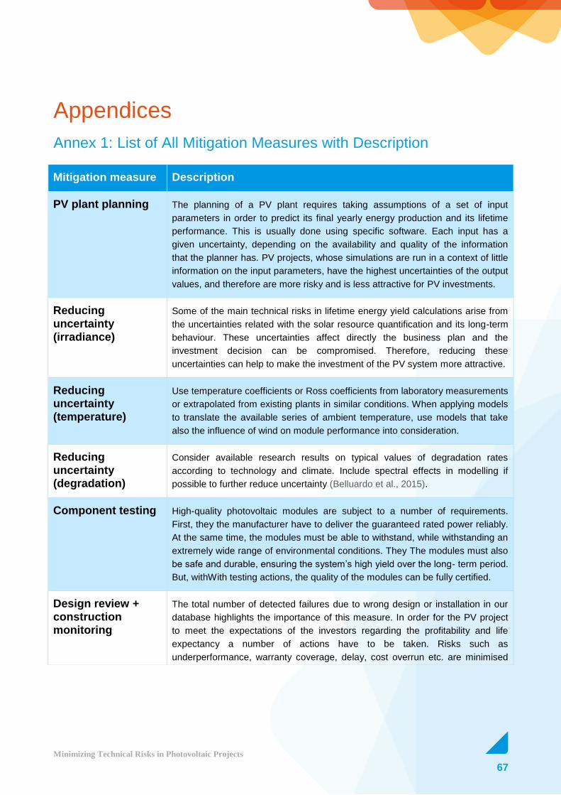
67
Minimizing Technical Risks in Photovoltaic Projects
Appendices
Annex 1: List of All Mitigation Measures with Description
Mitigation measure Description
PV plant planning The planning of a PV plant requires taking assumptions of a set of input
parameters in order to predict its final yearly energy production and its lifetime
performance. This is usually done using specific software. Each input has a
given uncertainty, depending on the availability and quality of the information
that the planner has. PV projects, whose simulations are run in a context of little
information on the input parameters, have the highest uncertainties of the output
values, and therefore are more risky and is less attractive for PV investments.
Reducing uncertainty (irradiance)
Some of the main technical risks in lifetime energy yield calculations arise from
the uncertainties related with the solar resource quantification and its long-term
behaviour. These uncertainties affect directly the business plan and the
investment decision can be compromised. Therefore, reducing these
uncertainties can help to make the investment of the PV system more attractive.
Reducing uncertainty (temperature)
Use temperature coefficients or Ross coefficients from laboratory measurements
or extrapolated from existing plants in similar conditions. When applying models
to translate the available series of ambient temperature, use models that take
also the influence of wind on module performance into consideration.
Reducing uncertainty (degradation)
Consider available research results on typical values of degradation rates
according to technology and climate. Include spectral effects in modelling if
possible to further reduce uncertainty (Belluardo et al., 2015).
Component testing High-quality photovoltaic modules are subject to a number of requirements.
First, they the manufacturer have to deliver the guaranteed rated power reliably.
At the same time, the modules must be able to withstand, while withstanding an
extremely wide range of environmental conditions. They The modules must also
be safe and durable, ensuring the system’s high yield over the long- term period.
But, withWith testing actions, the quality of the modules can be fully certified.
Design review + construction monitoring
The total number of detected failures due to wrong design or installation in our
database highlights the importance of this measure. In order for the PV project
to meet the expectations of the investors regarding the profitability and life
expectancy a number of actions have to be taken. Risks such as
underperformance, warranty coverage, delay, cost overrun etc. are minimised

68
Minimizing Technical Risks in Photovoltaic Projects
after the application of this measure.
Qualification of EPC
The qualification of EPC is a preventive mitigation measure that will reduce the
risk at an early stage of the PV project phase. EPC personell shall have a high
educational level as well as appropriate technical knowledge. Regular training
schemes should be designed and available to EPC personell for maintaining the
high quality of staff and service provision.
Advanced monitoring system
An advanced monitoring system allows the early detection and diagnosis of
faults. Early detection and diagnosis of faults during PV plant operation are
essential in order to obtain and maintain the energy yield high. Early remediation
of faults not only restores generation promptly but also avoids the occurrence of
additional component failures and leads to reduction of O&M costs. The benefit
of advanced monitoring is built up through reduced operational costs on one
hand and additional revenues resulting from a higher performance ratio and
higher availability on the other hand.
Basic monitoring system
A basic monitoring system typically allows the monitoring on plant level including
device alarm collection and notifications. Furthermore, aggregation functionality
on plant level for energy, irradiation and performance ratio are typically provided.
Advanced inspection
Advanced inspection relies on the use of techniques which go beyond visual
inspection such as infrared imaging (IR) and electroluminescence imaging (EL),
IV string analyser, etc.
Visual inspection Visual inspection can establish whether any visual changes are occurring that
may affect the performance of the principal components or reduce the effective
life of the system or components providing data needed for planning
maintenance and operation requirements. Through visual inspection technical
risks with high occurrence can be typically detected (inverter polluted air filter,
PV module glass breakage, broken connectors, etc).
Spare parts management
Spare parts management is a mitigation measure which has an impact in the
initial investment and can be applied to several components of a PV plant. An
effective spare parts management ensures the availability of the right amount
and type of components, equipment, parts, etc. either on site or in warehouses
or in manufacturers’ consignment stocks, for prompt replacement in case of
failure and/or to meet guarantees under O&M contracts.

69
Minimizing Technical Risks in Photovoltaic Projects
Annex 2: List of Impact of Applied Mitigation Measures on Risks
Component Risk
Modules Snail track High No No No No Medium Medium High
Modules Improperly installed No High Medium Low No Medium Medium High
Modules Glass breakage Medium Medium Low No No Medium Medium High
Modules Broken module No High Medium Medium No Medium Medium High
Modules Theft of modules No No No High High Medium Medium High
Modules Module damaged due to fire No No No High High Medium Medium High
Modules Failure bypass diode and junction box High No No High Medium Medium Medium High
Modules Shading No Low No High Medium Medium Medium No
Modules Soiling No No No High Medium Medium Medium No
Modules Cell cracks High Low No No No Medium No High
Modules Delamination Low No No No No Medium No High
Modules Defective backsheet High No No No No Medium Medium High
Modules Hotspot High No No No No Medium No High
Modules Missing modules No High Medium High No Medium Medium High
Modules EVA discoloration High No No No No Medium Medium High
Modules Corrosion in the junction box High No No No No Medium Medium High
Modules Corrosion of cell connectors High No No No No Medium Medium High
Modules Overheating junction box High No No No No Medium No High
Modules PID = Potential Induced degradation High No No No No Medium No High
Inverter Wrong installation No High Medium Medium No Medium Medium High
Inverter Inverter not operating (inverter failure or don't working after grid fault)No No No High Medium Medium Medium High
Inverter Wrong connection (positioning and numbering) No High Medium No No Medium Medium High
Inverter Inverter theft or vandalism No No No High Medium Medium Medium High
Inverter Inverter pollution No No No No No Medium Medium High
Inverter Burned supply cable and/or socket No No No High Medium Medium Medium High
Inverter Display off (broken or moisture inside of it) No No No No No Medium Medium High
Inverter Fault due to grounding issues, e.g. high humidity insideNo High Medium High Medium Medium Medium High
Inverter Inverter firmware issue No No No No No Medium Medium High
Inverter Data entry broken No No No No No Medium Medium High
Inverter Slow reaction time for warranty claims, Vague or inappropriate definition of procedure for warranty claimsNo No No No No Medium No High
Inverter Fan failure and overheating No Medium Medium High Medium Medium Medium High
Inverter Switch failure/damage No High Medium High Medium Medium Medium High
Inverter DC entry fuse failure causing or caused by array disconnectionNo No No High Medium Medium Medium High
Inverter Inverter damage due to lightning strike No High Medium High Medium Medium Medium High
Inverter Inverter wrongly sized No High Medium Medium No Medium Medium High
Inverter Error message No No No High Medium Medium Medium High
Inverter Polluted air filter - derating No No No High Medium Medium Medium High
Mounting structure Not proper installation No High Medium Medium No Medium Medium High
Mounting structure Wind damage No No No No No Medium Medium High
Mounting structure Tracker failure No Low No High Medium Medium Medium High
Mounting structure Corrosion No Low No No No Medium Medium High
Mounting structure Disallignment caused by ground instability No Medium Low No No Medium Medium High
Mounting structure Tracker maintenance No No No No No Medium Medium High
Mounting structure Oil leakage No Low No No No Medium Medium High
Mounting structure Corrosion of module clamps No Medium Low No No Medium Medium High
Connection & Distribution boxes Incorrect installation No High Medium No No Medium Medium High
Connection & Distribution boxes Main switch open and does not reclose again automaticallyNo No No High Medium Medium Medium High
Connection & Distribution boxes IP failure No High Medium No No Medium Medium High
Connection & Distribution boxes Broken/Wrong general switch No High Medium High Medium Medium Medium High
Connection & Distribution boxes General switch off No No No High Medium Medium Medium High
Connection & Distribution boxes Wrong wiring No High Medium No No Medium Medium High
Connection & Distribution boxes Cable gland missing or not installed correctly No High Medium No No Medium Medium High
Connection & Distribution boxes Missing protection No High Medium No No Medium Medium High
Connection & Distribution boxes Broken, missing or corroded cover No High Medium No No Medium Medium High
Connection & Distribution boxes Overcurrent protection not correctly sized No High Medium No No Medium Medium High
Connection & Distribution boxes UPS off/broken No No No No No Medium Medium High
Connection & Distribution boxes Wrong/Missing labeling No High Medium No No Medium Medium High
Cabling improper installation No High Medium No No Medium Medium High
Cabling Wrong/Absent cables connection No High Medium High Medium Medium Medium High
Cabling Broken/Burned connectors No Low No High Medium Medium Medium High
Cabling Wrong/absent cables No High Medium High Medium Medium Medium High
Cabling Damaged cable No No No High Medium Medium Medium High
Cabling Broken cable ties No High Medium No No Medium Medium High
Cabling Conduit failure No Medium Low No No Medium Medium High
Cabling Wrong connection, isolation and/or setting of strings No High Medium High Medium Medium Medium High
Cabling UV Aging No High Medium No No Medium Medium High
Cabling Cables undersized No High Medium No No Medium Medium No
Cabling Wrong wiring No High Medium No No Medium Medium High
Cabling Theft cables No No Low High Medium Medium Medium High
Transformer station & MV/HV Improper / Inadequate installation No High Medium No No Medium Medium High
Transformer station & MV/HV Broken transformer No No Low High High Medium Medium No
Transformer station & MV/HV Wrong transformer configuration No No Low High Medium Medium Medium No
Visual
Inspection
Spare Part
Managem
ent
Componen
t Testing
Design
Review +
constructio
Qualificati
on of EPC
Advanced
Monitorin
g system
Basic
Monitorin
g system
Advanced
Inspection

70
Minimizing Technical Risks in Photovoltaic Projects
Annex 3: Index of All Combinations

71
Minimizing Technical Risks in Photovoltaic Projects
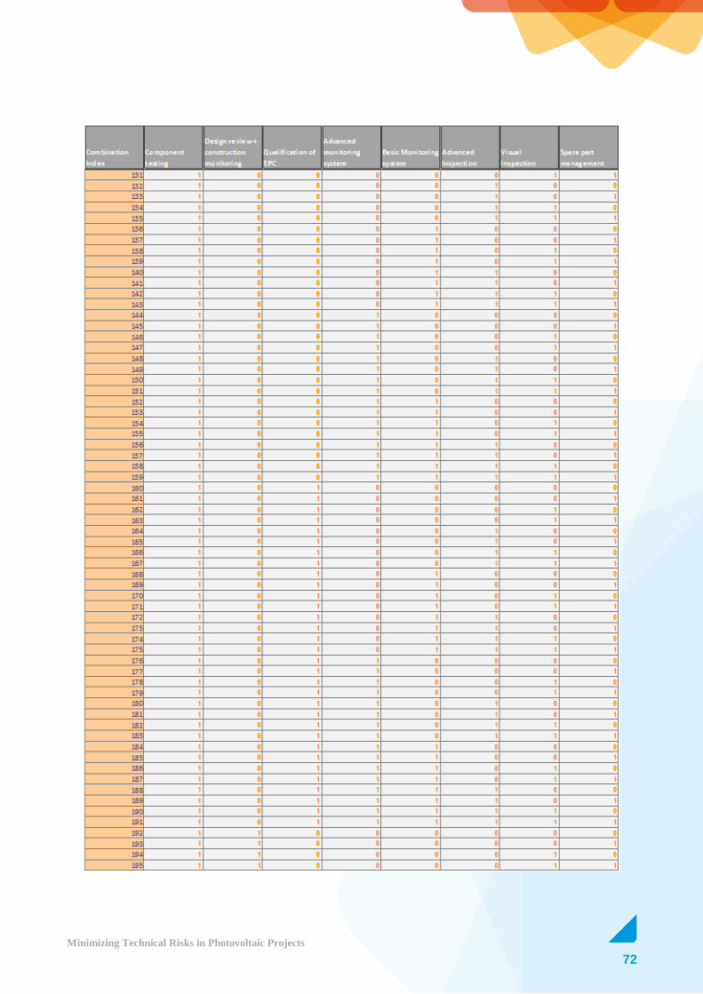
72
Minimizing Technical Risks in Photovoltaic Projects
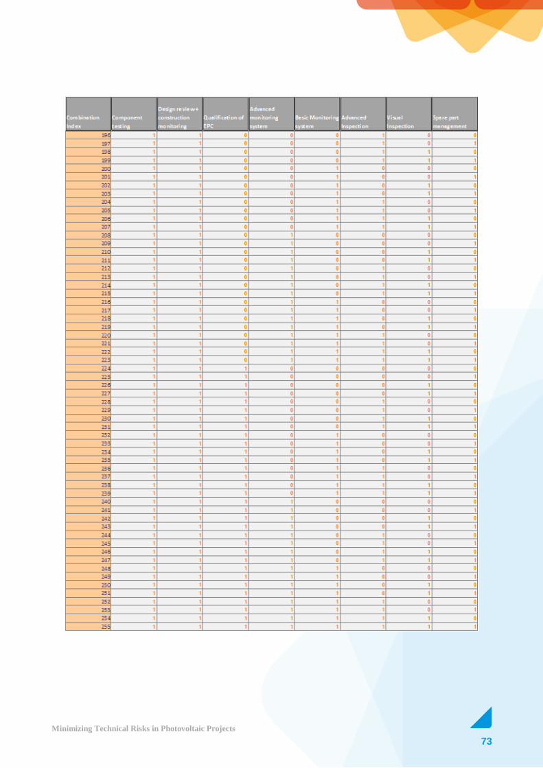
73
Minimizing Technical Risks in Photovoltaic Projects

74
Minimizing Technical Risks in Photovoltaic Projects
Annex 4: Uncertainty Values of Input and Output Parameters in the
Different Uncertainty Scenarios

75
Minimizing Technical Risks in Photovoltaic Projects
Annex 5: Examples of uncertainty reduction in the yield assessment
Figure A5.1: Impact of mitigation measures compared to the base scenario (fixed at 0)
Figure A5.2: Typical values of uncertainty reduction in relative terms for a few selected mitigation measures

76
Minimizing Technical Risks in Photovoltaic Projects
Figure A5.3: Example of uncertainty reduction (in relative terms) for a scenario where long term series of measured data on the
plane of array are available (low-end scenario)
Figure A5.4: Example of uncertainty reduction (in relative terms) where long term series of satellite data are combined with short
term series of measured data

77
Minimizing Technical Risks in Photovoltaic Projects

78
Minimizing Technical Risks in Photovoltaic Projects
This project has received funding from the European Union’s Horizon 2020 research
and innovation programme under grant agreement No 649997. The content of this
report reflects only the author’s view and the Commission is not responsible for any
use that may be made of the information it contains.
Funded by the Horizon 2020 Framework Programme of the European Union