Minimax optimal rates for Mondrian trees and forests

Jaouad Mourtada∗, Stephane Gaıffas†, Erwan Scornet‡

March 14, 2018

Abstract

Introduced by Breiman (2001), Random Forests are widely used as classification and re-gression algorithms. While being initially designed as batch algorithms, several variants havebeen proposed to handle online learning. One particular instance of such forests is the Mon-drian Forest (Lakshminarayanan et al., 2014, 2016), whose trees are built using the so-calledMondrian process, therefore allowing to easily update their construction in a streaming fash-ion. In this paper, we study Mondrian Forests in a batch setting and prove their consistencyassuming a proper tuning of the lifetime sequence. A thorough theoretical study of Mondrianpartitions allows us to derive an upper bound for the risk of Mondrian Forests, which turnsout to be the minimax optimal rate for both Lipschitz and twice differentiable regression func-tions. These results are actually the first to state that some particular random forests achieveminimax rates in arbitrary dimension, paving the way to a refined theoretical analysis andthus a deeper understanding of these black box algorithms.

1 Introduction

Originally introduced by Breiman (2001), Random Forests (RF) are state-of-the-art classificationand regression algorithms that proceed by averaging the forecasts of a number of randomizeddecision trees grown in parallel. Despite their widespread use and remarkable success in practicalapplications, the theoretical properties of such algorithms are still not fully understood (for anoverview of theoretical results on random forests, see Biau and Scornet, 2016). As a result ofthe complexity of the procedure, which combines sampling steps and feature selection, Breiman’soriginal algorithm has proved difficult to analyze. Consequently, most theoretical studies focus onmodified and stylized versions of Random Forests.

Among these methods, Purely Random Forests (PRF) (Breiman, 2000; Biau et al., 2008; Biau,2012; Genuer, 2012; Arlot and Genuer, 2014) that grow the individual trees independently of thesample, are particularly amenable to theoretical analysis. The consistency of such estimates (aswell as other idealized RF procedures) was first obtained by Biau et al. (2008), as a byproductof the consistency of individual tree estimates. A recent line of research (Scornet et al., 2015;Wager and Walther, 2015; Mentch and Hooker, 2016; Wager and Athey, 2017) has sought toobtain some theoretical guarantees for RF variants that more closely resembled the algorithm usedin practice. It should be noted, however, that most of these theoretical guarantees come at the priceof assumptions either on the data structure or on the Random Forest algorithm itself, being thusstill far from explaining the excellent empirical performance of Random Forests.∗CMAP, Ecole polytechnique, Universite Paris Saclay, Route de Saclay, 91128 Palaiseau cedex, France. Email:

jaouad.mourtada@polytechnique.edu†LPSM, Univ. Paris Diderot, batiment Sophie Germain, Paris, France and CMAP, Ecole Polytechnique, Universite

Paris Saclay, Route de Saclay, 91128 Palaiseau cedex, France. Email: stephane.gaiffas@lpsm.paris‡CMAP, Ecole Polytechnique, Universite Paris Saclay, Route de Saclay, 91128 Palaiseau cedex, France. Email:

erwan.scornet@polytechnique.edu

1

Another aspect of the theoretical study of random forests is to quantify the performance guar-antees by analyzing the bias/variance of simplified versions of Random Forests, such as PRFmodels (Genuer, 2012; Arlot and Genuer, 2014). In particular, Genuer (2012) shows that somePRF variants achieve the minimax rate for the estimation of a Lipschitz regression functions indimension one. The bias-variance analysis is extended in Arlot and Genuer (2014), showing thatPRF can also achieve minimax rates for C 2 regression functions in dimension one. The afore-mentioned rates of convergence are much more precise than mere consistency, and offer insightson the proper tuning of the procedure. Surprisingly, optimal rates are only obtained in the one-dimensional case (where decision trees reduce to histograms); only suboptimal rates are reachedin the higher dimensional setting, where trees exhibit a more intricate recursive structure.

From a more practical perspective, an important limitation of the most commonly used RF al-gorithms, such as Breiman’s Random Forests (Breiman, 2001) and the Extra-Trees algorithm (Geurtset al., 2006), is that they are typically trained in a batch manner, using the whole dataset, availableat once, to build the trees. In order to enable their use in situations when large amounts of datahave to be incorporated in a streaming fashion, several online variants of the decision trees andrandom forests algorithms have been proposed (Domingos and Hulten, 2000; Saffari et al., 2009;Taddy et al., 2011; Denil et al., 2013, 2014).

Of particular interest in this article is the Mondrian Forest algorithm, an efficient and accurateonline random forest classifier introduced by Lakshminarayanan et al. (2014) (see also Lakshmi-narayanan et al., 2016). This algorithm is based on the Mondrian process (Roy and Teh, 2009;Roy, 2011; Orbanz and Roy, 2015), a natural probability distribution on the set of recursive par-titions of the unit cube [0, 1]d. An appealing property of Mondrian processes is that they can beupdated in an online fashion: in Lakshminarayanan et al. (2014), the use of the conditional Mon-drian process enables to design an online algorithm which matches its batch counterpart: trainingthe algorithm one data point at a time leads to the same randomized estimator than if trained onthe whole dataset at once. The algorithm proposed in Lakshminarayanan et al. (2014) dependson a lifetime parameter λ that guides the complexity of the trees by stopping the tree buildingprocess. However, there are no theoretical insights to tune this parameter, which appears to be ofgreat importance in Mondrian Trees and Forests.

We study in this paper the Mondrian Forests in a batch setting and provide theoretical guidanceto tune the lifetime parameter. It turns out that allowing the lifetime parameter to depend on n at aproper rate results in the consistency of our proposed algorithm. Based on the detailed analysis ofMondrian partitions, we are able to derive the convergence rate of Mondrian Forests, which turnsout to be the minimax rate for Lipschitz and twice differentiable functions in arbitrary dimension.To the best of our knowledge, such results have only been proved for very specific purely randomforests, where the covariate space is of dimension one (Arlot and Genuer, 2014). Our analysis alsosheds light on the benefits of Mondrian Forests compared to a single Mondrian Tree.

Agenda. This paper is organized as follows. In Section 2, we describe in details the settingwe consider, and set the notations for trees and forests. Section 3 defines the Mondrian processintroduced by Roy and Teh (2009) and describes the Mondrian Forests algorithm; Section 4 isdevoted to the sharp properties established for Mondrian partitions that will be used throughoutthe rest of the paper to derive consistency and upper bounds which are minimax optimal. InSection 5, we prove statistical guarantees for Mondrian Forests, which provide us with a way totune the lifetime parameter. We also state that Mondrian Forests achieve the minimax rate forregression and classification and stress the optimality of forests, compared to individual trees.

2

2 Setting and notations

We first explain the general setting of the paper and describe the notations related to the Mondriantree structure. For the sake of conciseness, we consider the regression setting, and show how toextend the results to classification in Section 5 below.

Setting. We consider a regression framework, where the dataset Dn = {(X1, Y1), . . . , (Xn, Yn)}contains i.i.d. [0, 1]d × R-valued random variables, distributed as the generic pair (X,Y ), withE[Y 2] < ∞. This unknown distribution, characterized by the distribution µ of X on [0, 1]d andby the conditional distribution of Y |X , can be written as

Y = f(X) + ε, (1)

where f(X) = E[Y |X] is the conditional expectation of Y given X , and ε is a noise satisfyingE[ε|X] = 0. Our goal is to output a randomized estimate fn(·, Z,Dn) : [0, 1]d → R, where Zis a random variable that accounts for the randomization procedure; to simplify notation, we willgenerally denote fn(x, Z) = fn(x, Z,Dn). The quality of a randomized estimate fn is measuredby its quadratic risk

R(fn) = E[(fn(X,Z,Dn)− f(X))2]

where the expectation is taken with respect to (X,Z,Dn). We say that a sequence (fn)n>1 isconsistent whenever R(fn)→ 0 as n→∞.

Trees and Forests. LetM > 1 be the number of trees in a forest. We let fn(x, Z1), . . . , fn(x, ZM )be the randomized tree estimates at point x, associated to the same randomized mechanism, wherethe Zm are i.i.d. and correspond to the extra randomness introduced in the tree construction. SetZ(M) = (Z1, . . . , ZM ). The random forest estimate f (M)

n (x, Z(M)) is then defined by taking theaverage over all tree estimates fn(x, Zm), namely

f (M)n (x, Z(M)) =

1

M

M∑m=1

fn(x, Zm) . (2)

Let us now introduce some specific notations to describe the decision tree structure. A decisiontree (T,Σ) is composed of the following components:

• A finite rooted ordered binary tree T , with nodes N (T ), interior nodes N ◦(T ) and leavesL(T ) (so that N (T ) is the disjoint union of N ◦(T ) and L(T )). The nodes v ∈ N (T )are finite words on the alphabet {0, 1}, that is elements of the set {0, 1}∗ =

⋃n>0{0, 1}n:

the root ε of T is the empty word, and for every interior v ∈ {0, 1}∗, its left child is v0(obtained by adding a 0 at the end of v) while its right child is v1 (obtained by adding a 1at the end of v).

• A family of splits Σ = (σv)v∈N ◦(T ) at each interior node, where each split σv = (jv, sv)is characterized by its split dimension jv ∈ {1, . . . , d} and its threshold sv ∈ [0, 1].

Each randomized estimate fn(x, Zm) relies on a decision tree (T,Σ), the random variable Zm be-ing the random sampling of the tree structure T and of the splits (σv). This sampling mechanism,based on the Mondrian process, is defined in Section 3.

We associate to Π = (T,Σ) a partition (Cv)v∈L(T ) of the unit cube [0, 1]d, called a treepartition (or guillotine partition). For each node v ∈ N (T ), we define a hyper-rectangular regionCv recursively:

3

• The cell associated to the root of T is [0, 1]d;

• For each v ∈ N ◦(T ), we define

Cv0 := {x ∈ Cv : xjv 6 sjv} and Cv1 := Cv \ Cv0.

The leaf cells (Cv)v∈L(T ) form a partition of [0, 1]d by construction. In what follows, we willidentify a tree with splits (T,Σ) with its associated tree partition, and a node v ∈ N (T ) with thecell Cv ⊂ [0, 1]d. The Mondrian process, described in the next Section, defines a distribution overnested tree partitions, defined below.

Definition 1 (Nested tree partitions). A tree partition Π′ = (T ′,Σ′) is a refinement of the treepartition Π = (T,Σ) if every leaf cell of Π′ is contained in a leaf cell of Π′. This is equivalent tothe fact that T is a subtree of T ′ and, for every v ∈ N (T ) ⊆ N (T ′), σv = σ′v.

A nested tree partition is a family (Πt)t>0 of tree partitions such that, for every t, t′ ∈ R+ witht 6 t′, Πt′ is a refinement of Πt. Such a family can be described as follows: let T be the (in generalinfinite, and possibly complete) rooted binary tree, such thatN (T) =

⋃t>0N (Tt) ⊆ {0, 1}∗. For

each v ∈ N (T ), let τv = inf{t > 0 | v ∈ N (Tt)} < ∞ denote the birth time of the node v.Additionally, let σv be the value of the split σv,t in Πt for t > τv (which does not depend on tby the refinement property). Then, Π is completely characterized by T, Σ = (σv)v∈N (T) andT = (τv)v∈N (T).

The regression tree outputs a constant estimation of the label in each leaf cell Cv using asimple averaging of the labels Yi (1 6 i 6 n) such that Xi ∈ Cv.

3 The Mondrian Forest algorithm

The Mondrian process is a distribution on (infinite) nested tree partitions of the unit cube [0, 1]d

introduced by Roy and Teh (2009). This distribution enables us to define the Mondrian Foreststhat average the forecasts of Mondrian Trees obtained by sampling from the Mondrian processdistribution.

Given a rectangular box C =∏dj=1[aj , bj ] ⊆ Rd, we denote |C| :=

∑dj=1(bj − aj) its linear

dimension. The Mondrian process distribution MP(C) is a distribution on nested tree partitionsof C. To define it, we introduce the function ΦC , which maps any family of couples (ejv, u

jv) ∈

R+ × [0, 1] indexed by the coordinates j ∈ {1, . . . , d} and the nodes v ∈ {0, 1}∗ to a nested treepartition Π = ΦC((ejv, u

jv)v,j) of C. The splits σv = (jv, sv) and birth times τv of the nodes

v ∈ {0, 1}∗ are defined recursively, starting from the root ε:

• For the root node ε, we let τε = 0 and Cε = C.

• At each node v ∈ {0, 1}∗, given the labels of all its ancestors v′ @ v (so that in particularτv and Cv are determined), denote Cv =

∏dj=1[ajv, b

jv]. Then, select the split dimension

jv ∈ {1, . . . , d} and its location sv as follows:

jv = argmin16j6d

ejv

bjv − ajv, sv = ajvv + (bjvv − ajvv ) · ujvv , (3)

where we break ties in the choice of jv e.g. by choosing the smallest index j in the argmin.The node v is then split at time τv + ejvv /(b

jvv − ajvv ) = τv0 = τv1, we let Cv0 = {x ∈ Cv :

xjv 6 sv}, Cv1 = Cv \ Cv0 and recursively apply the procedure to its children v0 and v1.

4

1.3

2.3

2.7

3.2

•

•

••

••

−

−

−−−−

0

1.3

2.3

2.7

3.2λ=3.4

time

Figure 1: A Mondrian partition. The tree on the right-hand side (or equivalently the partition onthe left-hand side) is grown sequentially, where the split times are indicated on the vertical timeaxis.

For each λ ∈ R+, the tree partition Πλ = Φλ,C((ejv, ujv)v,j) is the pruning of Π at time λ,

obtained by removing all the splits in Π that occurred strictly after λ, so that the leaves of the treeare the maximal nodes (in the prefix order) v such that τv 6 λ. Figure 1 presents a particularinstance of Mondrian partition on a square box, with lifetime parameter λ = 3.4.

Definition 2 (Mondrian process). Let (Ejv, Ujv)v,j be a family of independent random variables,

with Ejv ∼ Exp(1), U jv ∼ U([0, 1]). The Mondrian process MP(C) on C is the distribution of therandom nested tree partition ΦC((Ejv, U

jv)v,j). In addition, we denote MP(λ,C) the distribution

of Φλ,C((Ejv, Ujv)v,j).

Sampling from MP(λ,C) can be done through the recursive procedure SampleMondrian(λ,C)of Algorithm 1.

Algorithm 1 SampleMondrian(λ,C) ; Sample a tree partition distributed as MP(λ,C).

1: Parameters: A rectangular box C ⊂ Rd and a lifetime parameter λ > 0.2: Call SplitCell(C, τ := 0, λ).

Algorithm 2 SplitCell(C, τ, λ) ; Recursively split a cell C, starting from time τ , until λ1: Parameters: A cell C =

∏16j6d[aj , bj ], a starting time τ and a lifetime parameter λ.

2: Sample an exponential random variable EC with intensity |C|.3: if τ + EC 6 λ then4: Draw at random a split dimension J ∈ {1, . . . , d}, with P(J = j) = (bj − aj)/|C|, and a

split threshold sJ uniformly in [aJ , bJ ].5: Split C along the split (J, sJ). Let C0 and C1 be the resulting cells.6: Call SplitCell(C0, τ + EC , λ) and SplitCell(C1, τ + EC , λ).7: else8: Do nothing.9: end if

Indeed, for any cell C =∏

16j6d[aj , bj ], if E1, . . . , Ed are independent exponential ran-dom variables with intensities b1 − a1, . . . , bd − ad, then EC = min16j6dEj is distributed asExp(

∑16j6d(bj − aj)) ∼ Exp(|C|). Moreover, if J = argmin16j6dEj , J and E are indepen-

dent and P[J = j] = (bj − aj)/|C|. These facts prove the equivalence between the definition of aMondrian process from Definition 2 and the construction described in Algorithms 1 and 2.

5

Remark 1. Using the memoryless property of exponential random variables (if E ∼ Exp(l) andλ > 0, the distribution of E − λ conditionally on {E > λ} is Exp(l)) it is possible to efficientlysample Πλ′ ∼ MP(λ′, C) given its pruning at time λ 6 λ′: Πλ ∼ MP(λ,C). This proves that theMondrian process is Markovian.

Finally, the procedure to build the Mondrian Forest is as follows: grow randomized tree par-titions Π

(1)λ , . . . ,Π

(M)λ , fit each one with the dataset Dn by averaging the labels falling into each

leaf (predicting 0 if the leaf is empty), then combine the resulting Mondrian Tree estimates byaveraging their predictions. In accordance with Equation (2), we let

f(M)λ,n (x, Z(M)) =

1

M

M∑m=1

f(m)λ,n (x, Zm) , (4)

be the Mondrian Forest estimate described above, where f (m)λ,n (x, Zm) denotes the Mondrian Tree

parametrized by the random variable Zm. Here, the variables Z1, . . . , ZM are independent anddistributed as the generic random variable Z = (Ejv, U

jv)v,j (see Definition 2).

4 Local and global properties of the Mondrian process

In this Section, we show that the properties of the Mondrian process enable to compute explicitlysome local and global quantities related to the structure of Mondrian partitions. To do so, we willneed the following two facts, exposed by Roy and Teh (2009).

Fact 1 (Dimension 1). For d = 1, the splits from a Mondrian process Πλ ∼ MP(λ, [0, 1]) form asubset of [0, 1], which is distributed as a Poisson point process of intensity λdx.

Fact 2 (Restriction). Let Πλ ∼ MP(λ, [0, 1]d) be a Mondrian partition, and C =∏dj=1[aj , bj ] ⊂

[0, 1]d be a box. Consider the restriction Πλ|C of Πλ on C, i.e. the partition on C induced by thepartition Πλ of [0, 1]d. Then Πλ|C ∼ MP(λ,C).

Fact 1 deals with the one-dimensional case by making explicit the distribution of splits forMondrian process, which follows a Poisson point process. The restriction property stated in Fact 2is fundamental, and enables to precisely characterize the behavior of the Mondrian partitions.

Given any point x ∈ [0, 1]d, the next Proposition 1 is a sharp result giving the exact distributionof the cell Cλ(x) containing x from the Mondrian partition. Such a characterization is typicallyunavailable for other randomized trees partitions involving a complex recursive structure.

Proposition 1 (Cell distribution). Let x ∈ [0, 1]d and denote by

Cλ(x) =∏

16j6d

[Lj,λ(x), Rj,λ(x)]

the cell of containing x in a partition Πλ ∼ MP(λ, [0, 1]d) (this cell corresponds to a leaf ). Then,the distribution of Cλ(x) is characterized by the following properties :

(i) L1,λ(x), R1,λ(x), . . . , Ld,λ(x), Rd,λ(x) are independent ;

(ii) For each j = 1, . . . , d, Lj,λ(x) is distributed as (x − λ−1Ej,L) ∨ 0 and Rj,λ(x) as (x +λ−1Ej,R) ∧ 1, where Ej,L, Ej,R ∼ Exp(1).

The proof of Proposition 1 is given in Section 7.1 below. Figure 2 is a graphical representationof Proposition 1. A consequence of Proposition 1 is next Corollary 1, which gives a precise upperbound on cell diameters, which will help in providing the approximation error of the MondrianTree and Forest in Section 5.

6

λ−1E1,L

λ−1E1,Rλ−1E2,L

λ−1E2,R

Cλ(x)

x

Figure 2: Cell distribution in a Mondrian partition. Proposition 1 specifies the distribution ofdistances between x and each side of the cell Cλ(x): distances are depicted by dashed lines andtheir distributions correspond to braces. These distances are independent truncated exponentialvariables.

Corollary 1 (Cell diameter). Set λ > 0. Let x ∈ [0, 1]d, and let Dλ(x) be the `2-diameter of thecell Cλ(x) containing x in a Mondrian partition Πλ ∼ MP(λ, [0, 1]d). For every δ > 0, we have

P(Dλ(x) > δ) 6 d

(1 +

λδ√d

)exp

(− λδ√

d

)and

E[Dλ(x)2

]6

4d

λ2.

In particular, if λ→∞, then Dλ(x)→ 0 in probability.

To control the risk of the Mondrian Tree and Mondrian Forest, we need an upper bound on thenumber of cells in a Mondrian partition. Quite surprisingly, this quantity can be computed exactly,as shown in Proposition 2.

Proposition 2 (Number of cells). If Kλ denotes the number of cells in a Mondrian Tree partitionΠλ ∼ MP(λ, [0, 1]d), we have E[Kλ] = (1 + λ)d.

The proof of Proposition 2, which is given in Section 7.1 below, it technically involved. It relieson a coupling argument: we introduce a recursive modification of the construction of the Mon-drian process which keeps the expected number of leaves unchanged, and for which this quantitycan be computed directly using the Mondrian-Poisson equivalence in dimension one (Fact 1). Amuch simpler result is E[Kλ] 6 (e(1 + λ))d, which was previously proposed in Mourtada et al.(2017). By contrast, Proposition 2 provides the exact value of this expectation, which removes asuperfluous ed factor. This significantly improves the dependency on d of the upper bounds statedin Theorems 2 and 3 below.

Remark 2. Proposition 2 naturally extends (with the same proof) to the more general case of aMondrian process with finite measures with no atoms ν1, . . . , νd on the sides C1, . . . , Cd of a boxC ⊆ Rd (for a definition of the Mondrian process in this more general case, see Roy, 2011). Inthis case, we have E [Kλ] =

∏16j6d(1 + νj(C

j)).

As illustrated in this Section, a remarkable fact with the Mondrian Forest is that the quantitiesof interest for the statistical analysis of the algorithm can be made explicit. In particular, we showthat a Mondrian partition is balanced enough so that it contains O(λd) cells of diameter O(1/λ),which is the minimal number of cells to cover [0, 1]d.

7

5 Minimax theory for Mondrian Forests

This Section gathers a universal consistency result and sharp upper bounds for the Mondrian Treesand Forests. Section 5.1 states the universal consistency of the procedure, provided that the life-time λn belongs to an appropriate range. Section 5.2 gives an upper bound valid for MondrianTrees and Forests which turns out to be minimax optimal for Lipschitz regression functions, pro-vided that λn is properly tuned. Finally, Section 5.3 shows that Mondrian Forests improve overMondrian trees, for twice continuously differentiable regression functions. Results for classifica-tion are given in Section 5.4.

5.1 Consistency of Mondrian Forests

The consistency of the Mondrian Forest, described in Algorithm 1, is established in Theorem 1below, provided a proper tuning of the lifetime parameter λn.

Theorem 1 (Universal consistency). Assume that E[Y 2] <∞. Let λn →∞ such that λdn/n→ 0.Then, Mondrian tree estimates (whose construction is described in Algorithm 1) with lifetimeparameter λn are consistent. As a consequence, Mondrian Forests estimates with M > 1 treesand lifetime parameter λn are consistent.

The proof of Theorem 1 is given in Section 7.2. This consistency result is universal, in thesense that it makes no assumption on the joint distribution of (X,Y ), apart from the fact thatE[Y 2] < ∞, which is necessary to ensure that the quadratic risk is well-defined. This contrastswith several consistency results on Random Forests (see, e.g., Breiman, 2004; Biau, 2012) whichassume that the density of X is bounded from below and above. The proof of Theorem 1 uses theproperties of Mondrian partitions established in Section 4, in conjunction with general consistencyresults for histograms.

The only parameter in Mondrian Tree is the lifetime λn, which encodes the complexity of thetrees. Requiring an assumption on this parameter is natural, and confirmed by the well-knownfact that the tree-depth is an important tuning parameter for Random Forests (see, for instance,Biau and Scornet, 2016). However, Theorem 1 leaves open the question of a theoretically optimaltuning of λn under additional assumptions on the regression function f , which we address in thefollowing sections.

5.2 Mondrian Trees and Forests are minimax over the class of Lipschitz functions

The bounds obtained in Corollary 1 and Proposition 2 are explicit and sharp in their dependencyon λ. Based on these properties, we now establish a theoretical upper bound on the risk of Mon-drian Trees, which gives the optimal theoretical tuning of the lifetime parameter λn. To pursue theanalysis, we work under the following

Assumption 1. Assume that (X,Y ) satisfies Equation (1) where Y satisfies E(Y 2) <∞, where εis a real-valued random variable such that E(ε |X) = 0 and Var(ε |X) 6 σ2 <∞ almost surely.

Theorem 2 states an upper bound on the risk of Mondrian Trees and Forests, which explicitlydepends on the lifetime parameter λ. Selecting λ that minimizes this bound leads to a convergencerate which turns out to be minimax optimal over the class of Lipschitz functions (see e.g. ChapterI.3 in Nemirovski (2000) for details on minimax rates).

Theorem 2. Grant Assumption 1 and assume that f is L-Lipschitz. Let M > 1. The quadraticrisk of the Mondrian Forest f (M)

λ,n with lifetime parameter λ > 0 satisfies

E[(f

(M)λ,n (X)− f(X))2

]6

4dL2

λ2+

(1 + λ)d

n

(2σ2 + 9‖f‖2∞

). (5)

8

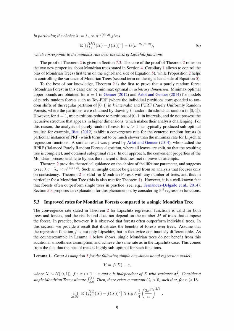
In particular, the choice λ := λn � n1/(d+2) gives

E[(f

(M)λn,n

(X)− f(X))2]

= O(n−2/(d+2)), (6)

which corresponds to the minimax rate over the class of Lipschitz functions.

The proof of Theorem 2 is given in Section 7.3. The core of the proof of Theorem 2 relies onthe two new properties about Mondrian trees stated in Section 4. Corollary 1 allows to control thebias of Mondrian Trees (first term on the right-hand side of Equation 5), while Proposition 2 helpsin controlling the variance of Mondrian Trees (second term on the right-hand side of Equation 5).

To the best of our knowledge, Theorem 2 is the first to prove that a purely random forest(Mondrian Forest in this case) can be minimax optimal in arbitrary dimension. Minimax optimalupper bounds are obtained for d = 1 in Genuer (2012) and Arlot and Genuer (2014) for modelsof purely random forests such as Toy-PRF (where the individual partitions corresponded to ran-dom shifts of the regular partition of [0, 1] in k intervals) and PURF (Purely Uniformly RandomForests, where the partitions were obtained by drawing k random thresholds at random in [0, 1]).However, for d = 1, tree partitions reduce to partitions of [0, 1] in intervals, and do not possess therecursive structure that appears in higher dimensions, which makes their analysis challenging. Forthis reason, the analysis of purely random forests for d > 1 has typically produced sub-optimalresults: for example, Biau (2012) exhibit a convergence rate for the centered random forests (aparticular instance of PRF) which turns out to be much slower than the minimax rate for Lipschitzregression functions. A similar result was proved by Arlot and Genuer (2014), who studied theBPRF (Balanced Purely Random Forests algorithm, where all leaves are split, so that the resultingtree is complete), and obtained suboptimal rates. In our approach, the convenient properties of theMondrian process enable to bypass the inherent difficulties met in previous attempts.

Theorem 2 provides theoretical guidance on the choice of the lifetime parameter, and suggeststo set λ := λn � n1/(d+2). Such an insight cannot be gleaned from an analysis that focuses onlyon consistency. Theorem 2 is valid for Mondrian Forests with any number of trees, and thus inparticular for a Mondrian Tree (this is also true for Theorem 1). However, it is a well-known factthat forests often outperform single trees in practice (see, e.g., Fernandez-Delgado et al., 2014).Section 5.3 proposes an explanation for this phenomenon, by considering C 2 regression functions.

5.3 Improved rates for Mondrian Forests compared to a single Mondrian Tree

The convergence rate stated in Theorem 2 for Lipschitz regression functions is valid for bothtrees and forests, and the risk bound does not depend on the number M of trees that composethe forest. In practice, however, it is observed that forests often outperform individual trees. Inthis section, we provide a result that illustrates the benefits of forests over trees. Assume thatthe regression function f is not only Lipschitz, but in fact twice continuously differentiable. Asthe counterexample in Lemma 1 below shows, single Mondrian trees do not benefit from thisadditional smoothness assumption, and achieve the same rate as in the Lipschitz case. This comesfrom the fact that the bias of trees is highly sub-optimal for such functions.

Lemma 1. Grant Assumption 1 for the following simple one-dimensional regression model:

Y = f(X) + ε,

where X ∼ U([0, 1]), f : x 7→ 1 + x and ε is independent of X with variance σ2. Consider asingle Mondrian Tree estimate f (1)

λ,n. Then, there exists a constant C0 > 0, such that, for n > 18,

infλ∈R∗+

E[(f

(1)λ,n(X)− f(X))2

]> C0 ∧

1

4

(3σ2

n

)2/3

.

9

The proof of Lemma 1 is given in Section 7.4. Since the minimax rate over the class of C 2

functions in dimension 1 isO(n−4/5), Lemma 1 proves that a single Mondrian Tree is not minimaxoptimal for the class of C 2 functions.

However, it turns out that large enough Mondrian Forests, which average Mondrian trees, areminimax optimal for C 2 functions. Therefore, Theorem 3 below highlights the benefits of a forestcompared to a single tree.

Theorem 3. Grant Assumption 1 and assume that X has a positive and Cp-Lipschitz density pw.r.t the Lebesgue measure on [0, 1]d and that the regression function f is C 2 on [0, 1]d. Let f (M)

λ,n

be the Mondrian Forest estimate composed of M > 1 trees, with lifetime parameter λ. Then, thefollowing upper bound holds for every ε ∈ [0, 1/2):

E[(f(M)λ,n (X)−f(X))2 |X ∈ [ε, 1− ε]d] 6 8d‖∇f‖2∞

Mλ2+

2(1 + λ)d

n

2σ2 + 9‖f‖2∞p0(1− 2ε)d

+72d‖∇f‖2∞p1

p0(1− 2ε)de−λε

λ3+

72d3‖∇f‖2∞C2pp

21

p40

1

λ4+

4d2‖∇2f‖2∞p21

p20

1

λ4, (7)

where p0 = inf [0,1]d p, p1 = sup[0,1]d p, ‖∇f‖∞ = supx∈[0,1]d ‖∇f(x)‖2 and ‖∇2f‖∞ =

supx∈[0,1]d ‖∇2f(x)‖op, with ‖ · ‖op the operator norm. In particular, the choices λn � n1/(d+4)

and Mn & n2/(d+4) give

E[(f

(Mn)λn,n

(X)− f(X))2 |X ∈ [ε, 1− ε]d]

= O(n−4/(d+4)), (8)

which corresponds to the minimax rate over the set of C 2 functions. Besides, letting λn � n1/(d+3)

andMn & n2/(d+3) yields the following upper bound on the integrated risk of the Mondrian Forestestimate over the whole hypercube [0, 1]d,

E[(f

(Mn)λn,n

(X)− f(X))2]

= O(n−3/(d+3)). (9)

The proof of Theorem 3 is given in Section 7.5 below. It relies on an improved control ofthe bias, compared to what we did in Theorem 2 in the Lipschitz case: it exploits the knowledgeof the distribution of the cell Cλ(x) given in Proposition 1 instead of merely the cell diametergiven in Corollary 1 (which was enough for Theorem 2). The improved rate for Mondrian Forestscompared to Mondrian trees comes from the fact that large enough forests smooth the decisionfunction of single trees, which are discontinuous piecewise constant functions, and therefore can-not approximate smooth functions well enough. This was already noticed in Arlot and Genuer(2014) for purely random forests.

Remark 3. While Equation (8) gives the minimax minimax rate for C 2 function, it suffers from anunavoidable standard artifact, namely the boundary effect which affects local averaging estimates,such as kernel estimators, see Wasserman (2006) and Arlot and Genuer (2014). It is howeverpossible to set ε = 0 in Equation (7), which leads to the sub-optimal rate stated in (9).

Let us now consider, as a by-product of the analysis conducted for regression estimation, thesetting of binary classification.

5.4 Results for binary classification

Assume that we are given a dataset Dn = {(X1, Y1), . . . , (Xn, Yn)} of i.i.d. [0, 1]d×{0, 1}-valuedrandom variables, distributed as a generic pair (X,Y ) and define η(x) = P[Y = 1|X = x].

10

We define the Mondrian Forest classifier g(M)λ,n as a plug-in estimator of the regression estimator.

Namely, we introduceg

(M)λ,n (x) = 1{f (M)

λ,n (x)>1/2}

for all x ∈ [0, 1]d, where f (M)λ,n is the Mondrian Forest estimate defined in the regression setting.

The performance of g(M)λ,n is assessed by the 0-1 classification error defined as

L(g(M)λ,n ) = P[g

(M)λ,n (X) 6= Y ], (10)

where the probability is taken with respect to (X,Y, Z(M),Dn). Note that (10) is larger than theBayes risk defined as

L(g?) = P[g?(X) 6= Y ],

where g?(x) = 1{η(x)>1/2}. A general theorem (Theorem 6.5 in Devroye et al. (1996)) allows

us to derive an upper bound on the distance between the classification risk of g(M)λ,n and the Bayes

risk, based on Theorem 2.

Corollary 2. Let M > 1 and assume that η is Lipschitz. Then, the Mondrian Forest classifierg

(M)λn,n

with lifetime parameter λn � n1/(d+2) satisfies

L(g(M)λn,n

)− L(g?) = o(n−1/(d+2)).

The rate of convergence o(n−1/(d+2)) for the error probability with a Lipschitz conditionalprobability η is optimal (Yang, 1999). We can also extend in the same way Theorem 3 to thecontext of classification. This is done in the next Corollary.

Corollary 3. In the classification framework described in Section 5.2, assume that X has a pos-itive and Lipschitz density p w.r.t the Lebesgue measure on [0, 1]d and that the conditional proba-bility η is C 2 on [0, 1]d. Let g(Mn)

λn,nbe the Mondrian Forest classifier composed of Mn & n2/(d+4)

trees, with lifetime λn � n1/(d+4). Then, for all ε ∈ [0, 1/2),

P[g(Mn)λn,n

(X) 6= Y |X ∈ [ε, 1− ε]d]− P[g?(X) 6= Y |X ∈ [ε, 1− ε]d] = o(n−2/(d+4)). (11)

This shows that Mondrian Forests achieve an improved rate compared to Mondrian trees forclassification.

6 Conclusion

Despite their widespread use in practice, the theoretical understanding of Random Forests is stillincomplete. In this work, we show that the Mondrian Forest, originally introduced to provide anefficient online algorithm, leads to an algorithm that is not only consistent, but in fact minimaxoptimal under nonparametric assumptions in arbitrary dimension. This is to the best of our knowl-edge, the first time such a result is obtained for a random forest method in arbitrary dimension.Besides, our analysis allows to illustrate improved rates for forests compared to individual trees.Mondrian partitions possess nice geometric properties, which we were able to control in a sharpand direct fashion, while previous approaches (Biau et al., 2008; Arlot and Genuer, 2014) requirearguments that work conditionally on the structure of the tree. This suggests that Mondrian Forestscan be viewed as an optimal variant of purely random forests, which could set a foundation formore sophisticated and theoretically sound random forest algorithms.

11

The optimal upper boundO(n−4/(d+4)) obtained in this paper is very slow when the number offeatures d is large. This comes from the well-known curse of dimensionality phenomenon, a prob-lem affecting all fully nonparametric algorithms. A standard approach used in high-dimensionalsettings is to work under a sparsity assumption, where only s � d features are informative. Adirection for future work could be to improve Mondrian Forests using a data-driven choice of thefeatures along which the splits are performed, reminiscent of Extra-Trees (Geurts et al., 2006).From a theoretical perspective, it would be interesting to see how minimax rates obtained here canbe combined with results on the ability of forests to select informative variables (see, for instance,Scornet et al., 2015).

7 Proofs

7.1 Proofs of Propositions 1 and 2 and of Corollary 1

Proof of Proposition 1. Let 0 6 a1, . . . , an, b1, . . . , bn 6 1 be such that aj 6 xj 6 bj for 1 6j 6 d. Let A :=

∏dj=1[aj , bj ]. Note that the event

{L1,λ(x) 6 a1, R1,λ(x) > b1, . . . , Ld,λ(x) 6 ad, Rd,λ(x) > bd}

coincides — up to the negligible event that one of the splits of Πλ occurs on coordinate j at ajor bj — with the event that Πλ does not cut C, i.e. that the restriction Πλ|C of Πλ to C containsno split. Now, by the restriction property of the Mondrian process (Fact 2), Πλ|C is distributed asMP(λ,A) ; in particular, the probability that Πλ|C contains no split is exp(−λ|A|). Hence, wehave

P(L1,λ(x) 6 a1, R1,λ(x) > b1, . . . , Ld,λ(x) 6 ad, Rd,λ(x) > bd)

= exp(−λ(x− a1)) exp(−λ(b1 − x)) · · · exp(−λ(x− ad)) exp(−λ(bd − x)) . (12)

In particular, setting aj = bj = x in (12) except for one aj or bj , and using that Lλ,j(x) 6 x andRλ,j(x) > x, we obtain

P(Rj,λ(x) > bj) = exp(−λ(bj − x)) and P(Lj,λ(x) 6 aj) = exp(−λ(x− aj)) . (13)

Since clearly Rj,λ(x) 6 1 and Lj,λ(x) > 0, equation (13) implies (ii). Additionally, pluggingequation (13) back into equation (12) shows that L1,λ(x), R1,λ(x), . . . , Ld,λ(x), Rd,λ(x) are inde-pendent, i.e. point (i). This completes the proof.

Proof of Corollary 1. By Proposition 1, D1λ(x) = R1

λ(x) − x1 + x1 − L1λ(x) is stochastically

upper bounded by λ−1(E1 + E2) with E1, E2 two independent Exp(1) random variables, whichis distributed as Gamma(2, λ). This implies that, for every δ > 0,

P(D1λ(x) > δ) 6 (1 + λδ)e−λδ (14)

(with equality if δ 6 x1∧ (1−x1)), and E[D1λ(x)2] 6 λ−2(E[E2

1 ] +E[E22 ]) = 4

λ2. The bound (1)

for the diameter Dλ(x) =√∑d

j=1Djλ(x)2 follows from the observation that

P(Dλ(x) > δ) 6 P(∃j : Dj

λ(x) >δ√d

)6 dP

(D1λ(x) >

δ√d

),

while the bound (1) is obtained by noting that E[Dλ(x)2] = dE[D1λ(x)2].

12

Proof of Proposition 2. At a high level, the idea of the proof is to modify the construction of theMondrian partition (and hence, the distribution of the underlying process) without affecting theexpected number of cells. More precisely, we show a recursively way to transform the Mondrianprocess that breaks the underlying independence structure but leaves E[Kλ] unchanged, and whicheventually leads to a random partition Πλ for which this quantity can be computed directly andequals (1 + λ)d.

We will in fact show the result for a general box C (not just the unit cube). The proof proceedsin two steps:

1. Define a modified process Π, and show that E[Kλ

]=∏dj=1(1 + λ|Cj |).

2. It remains to show that E [Kλ] = E[Kλ

]. For this, it is sufficient to show that the distribution

of the birth times τv and τv of the node v is the same for both processes. This is done byinduction on v, by showing that the splits at one node of both processes have the sameconditional distribution given the splits at previous nodes.

Let (Ejv, Ujv)v∈{0,1}∗,16j6d be a family of independent random variables with Ejv ∼ Exp(1)

and U jv ∼ U([0, 1]). By definition, Π = ΦC((Ejv, Ujv)v,j) (ΦC being defined in Section 3) follows

a Mondrian process distribution MP(C). Denote for every node v ∈ {0, 1}∗ Cv the cell of v, τv itsbirth time, as well as its split time Tv, dimension Jv, and threshold Sv (note that Tv = τv0 = τv1).In addition, for every λ ∈ R+, denote Πλ ∼ MP(λ,C) the tree partition restricted to the time λ,and Kλ ∈ N ∪ {+∞} its number of nodes.

Construction of the modified process. Now, consider the following modified nested partitionof C, denoted Π, and defined through its split times, dimension and threshold Tv, Jv, Sv (whichdetermine the birth times τv and cells Cv), and current j-dimensional node vj(v) ∈ {0, 1}∗ (1 6j 6 d) at each node v. First, for every j = 1, . . . , d, let Π′j = ΦCj ((E

jv, U

jv)v∈{0,1}∗) ∼ MP(Cj)

be the nested partition of the interval Cj determined by (Ejv, Ujv)v; its split times and thresholds

are denoted (S′jv , T′jv ). Then, Π is defined recursively as follows:

• At the root node ε, let τε = 0 and Cε = C, as well as vj(ε) := ε for j = 1, . . . , d.

• At any node v, given (τv′ , Cv′ ,vj(v′))v′vv (i.e., given (Jv′ , Sv′ , Tv′)v′@v) define:

Tv = min16j6d

T ′jvj(v), Jv := argmin16j6d

T ′jvj(v), Sv = S′jvj(v) (15)

as well as

vj(va) =

{vj(v)a if j = Jv

vj(v) else.(16)

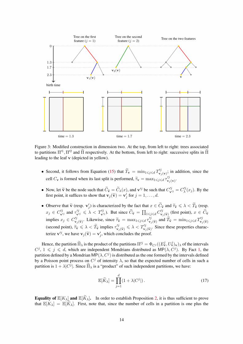
Finally, for every λ ∈ R+, define Πλ and Kλ as before from Π. This construction is illustrated inFigure 3.

Computation of E[Kλ]. Now, it can be seen that the partition Πλ is a rectangular grid which isthe “product” of the partitions Π′j of the intervals Cj , 1 6 j 6 d. Indeed, let x ∈ [0, 1]d, andlet Cλ(x) be the cell in Πλ that contains x; we need to show that Cλ(x) =

∏dj=1C

′jλ (x), where

C ′jλ (x) is the subinterval of Cj in the partition Π′j that contains xj . The proof proceeds in severalsteps:

• First, Equation (15) shows that, for every node v, we have Cv =∏

16j6dC′jvj(v), since the

successive splits on the j-th coordinate of Cv are precisely the ones of C ′jvj(v).

13

−

birth time

−−

−

0

1.3

1.7

2.3

Tree on the firstfeature (j = 1)

Tree on the secondfeature (j = 2)

Tree on the two features

•v

•

• • ••••

•

•v1(v)

•

• •

•

•v2(v)

•

•

time = 1.3 time = 1.7 time = 2.3

Figure 3: Modified construction in dimension two. At the top, from left to right: trees associatedto partitions Π′1,Π′2 and Π respectively. At the bottom, from left to right: successive splits in Πleading to the leaf v (depicted in yellow).

• Second, it follows from Equation (15) that Tv = min16j6d T′jvj(v); in addition, since the

cell Cv is formed when its last split is performed, τv = max16j6d τ′jvj(v).

• Now, let v be the node such that Cv = Cλ(x), and v′j be such that C ′jv′j

= C ′jλ (xj). By thefirst point, it suffices to show that vj(v) = v′j for j = 1, . . . , d.

• Observe that v (resp. v′j) is characterized by the fact that x ∈ Cv and τv 6 λ < Tv (resp.xj ∈ C ′j

v′jand τ ′j

v′j6 λ < T ′j

v′j). But since Cv =

∏16j6dC

′jvj(v) (first point), x ∈ Cv

implies xj ∈ C ′jvj(v). Likewise, since τv = max16j6d τ′jvj(v) and Tv = min16j6d T

′jvj(v)

(second point), τv 6 λ < Tv implies τ ′jvj(v) 6 λ < T ′jvj(v). Since these properties charac-

terize v′j , we have vj(v) = v′j , which concludes the proof.

Hence, the partition Πλ is the product of the partitions Π′j = ΦCj ((Ejv, U

jv)v)λ of the intervals

Cj , 1 6 j 6 d, which are independent Mondrians distributed as MP(λ,Cj). By Fact 1, thepartition defined by a Mondrian MP(λ,Cj) is distributed as the one formed by the intervals definedby a Poisson point process on Cj of intensity λ, so that the expected number of cells in such apartition is 1 + λ|Cj |. Since Πλ is a “product” of such independent partitions, we have:

E[Kλ] =

d∏j=1

(1 + λ|Cj |) . (17)

Equality of E[Kλ] and E[Kλ]. In order to establish Proposition 2, it is thus sufficient to provethat E[Kλ] = E[Kλ]. First, note that, since the number of cells in a partition is one plus the

14

number of splits (as each split increases the number of cells by one)

Kλ = 1 +∑

v∈{0,1}∗1(Tv 6 λ)

so thatE[Kλ] = 1 +

∑v∈{0,1}∗

P(Tv 6 λ) (18)

and, likewise,E[Kλ] = 1 +

∑v∈{0,1}∗

P(Tv 6 λ) . (19)

Therefore, it suffices to show that P(Tv 6 λ) = P(Tv 6 λ) for every v ∈ {0, 1}∗ and λ > 0, i.e.that Tv and Tv have the same distribution for every v.

In order to establish this, we show that, for every v ∈ {0, 1}∗, the conditional distribution of(Tv, Jv, Sv) given Fv = σ((Tv′ , Jv′ , Sv′),v

′ @ v) has the same form as the conditional distribu-tion of (Tv, Jv, Sv) given Fv = σ((Tv′ , Jv′ , Sv′),v

′ @ v), in the sense that there exits a family ofconditional distributions (Ψv)v such that, for every v, the conditional distribution of (Tv, Jv, Sv)given Fv = σ((Tv′ , Jv′ , Sv′),v

′ @ v) is Ψv(·|(Tv′ , Jv′ , Sv′),v′ @ v) and the conditional distri-bution of (Tv, Jv, Sv) given Fv = σ((Tv′ , Jv′ , Sv′),v

′ @ v) is Ψv(·|(Tv′ , Jv′ , Sv′),v′ @ v).First, recall that the variables (Ejv′ , U

jv′)v′∈{0,1}∗,16j6d are independent, so that (Ejv, U

jv)16j6d

is independent from Fv ⊆ σ((Ejv′ , Ujv′)v′@v,16j6d). As a result, conditionally on Fv, the

Ejv, Ujv, 1 6 j 6 d are independent variables with Ejv ∼ Exp(1) and U jv ∼ U([0, 1]), Also,

recall that if T1, . . . , Td are independent exponential random variables of intensities λ1, . . . , λd,and if T = min16j6d Tj and J = argmin16j6d Tj , then P(J = j) = λj/

∑dj′=1 λj′ , T ∼

Exp(∑d

j=1 λj) and J and T are independent. Hence, conditionally on Fv, Tv−τv = min16j6dEjv/|Cjv| ∼

Exp(∑d

j=1 |Cjv|) = Exp(|Cv|), Jv := argmin16j6dE

jv/|Cjv| equals j with probability |Cjv|/|Cv|,

Tv, Jv are independent and (Sv|Tv, Jv) ∼ U(CJvv ).Now consider the conditional distribution of (Tv, Jv, Sv) given Fv. Let (vv)v∈N be a path

in {0, 1}∗ from the root: v0 := ε, vv+1 is a child of vv for v ∈ N, and vv v v for 0 6 v 6depth(v). Define for v ∈ N, Ejv = Ejvv and U jv = U jvv if vv+1 is the left child of vv, and1 − U jvv otherwise. Then, the variables (Ejv, U

jv )v∈N,16j6d are independent, with Ejv ∼ Exp(1),

U jv ∼ U([0, 1]), so that the hypotheses of Technical Lemma 1 apply. In addition, note that,with the notations of Technical Lemma 1, a simple induction shows that Jv = Jvv , Tv = Tvv ,Uv = Uvv and Ljv = |Cjvv |, so that Fv = Fvv . Applying Technical Lemma 1 for v = depth(v)(so that vv = v) therefore gives the following: conditionally on Fv, Tv, Jv, Uv are independent,Tv − τv ∼ Exp(|Cjv|), P(Jv = j |Fv) = |Cjv|/

(∑dj′=1 |C

jv|)

and Uv ∼ U([0, 1]), so that

(Sv|Fv, Tv, Jv) ∼ U(C Jvv ).Hence, we have proven that, for every v ∈ {0, 1}∗, the conditional distribution of (Tv, Jv, Sv)

given Fv = σ((Tv′ , Jv′ , Sv′),v′ @ v) has the same form as that of (Tv, Jv, Sv) given Fv =

σ((Tv′ , Jv′ , Sv′),v′ @ v). By induction on v, since Fε = Fε is the trivial σ-algebra, this implies

that the distribution of Tv is the same as that of Tv for every v. Plugging this into Equations (18)and (19) and combining it with (17) completes the proof of Proposition 2.

Technical Lemma 1. Let (Ejv, Ujv )v∈N?,16j6d be a family of independent random variables, with

U jv ∼ U([0, 1]) and Ejv ∼ Exp(1). Let a1, . . . , ad > 0. For 1 6 j 6 d, define the sequence(T jv , L

jv)v∈N as follows:

• Lj0 = aj , Tj0 =

Ej0aj

;

15

• for v ∈ N, Ljv+1 = U jvLjv, T jv+1 = T jv +

Ejv+1

Ljv+1

.

Define recursively the variables V jv (v ∈ N, 1 6 j 6 d) as well as Jv, Tv, Uv (v ∈ N) as follows:

• V j0 = 0 for j = 1, . . . , d.

• for v ∈ N, given V jv (1 6 j 6 d), denoting T jv = T j

V jvand U jv = U j

V jv, set

Jv = argmin16j6d

T jv , Tv = min16j6d

T jv = T Jvv , Uv = U Jvv , V jv+1 = V j

v +1(Jv = j).

(20)

Then, the conditional distribution of (Jv, Tv, Uv) given Fv = σ((Jv′ , Tv′ , Uv′), 0 6 v′ < v) is thefollowing (denoting Ljv = Lj

V jv): Jv, Tv, Uv are independent, P(Jv = j |Fv) = Ljv/(

∑dj′=1 L

j′v ),

Tv − Tv−1 ∼ Exp(∑d

j=1 Ljv) (with the convention T−1 = 0) and Uv ∼ U([0, 1]).

Proof of Technical Lemma 1. We show by induction on v ∈ N the following property: condition-ally on Fv, (T jv , U

jv )16j6d are independent, T jv − Tv−1 ∼ Exp(Ljv) and U jv ∼ U([0, 1]).

Initialization For v = 0 (with F0 the trivial σ-algebra), since V j0 = 0 we have T j0 = Ej0/aj ∼

Exp(aj) = Exp(Lj0), U j0 = U j0 ∼ U([0, 1]) and these random variables are independent.

Inductive step Let v ∈ N, and assume the property is true up to step v. Conditionally on Fv+1,i.e. on Fv, Tv, Jv, Uv, we have:

• for j 6= Jv, the variables T jv+1 − Tv−1 = T jv − Tv−1 are independent Exp(Ljv) =

Exp(Ljv+1) random variables (when conditioned only on Fv, by the induction hypoth-esis), conditioned on T jv+1 − Tv−1 > Tv − Tv−1, so by the memory-less property ofexponential random variables T jv+1−Tv = (T jv+1−Tv−1)−(Tv−Tv−1) ∼ Exp(Ljv+1)(and those variables are independent).

• for j 6= Jv, the variables U jv+1 = U jv are independent U([0, 1]) random variables(conditionally on Fv), conditioned on the independent variables Tv, Jv, Uv, so theyremain independent U([0, 1]) random variables.

• (T Jvv+1− Tv, UJvv+1) = (EJv

V Jvv+1

/LJvv+1, UJv

V Jvv+1

) is distributed, conditionally on Fv+1, i.e.

on Jv, Tv, V Jvv+1, L

Jvv+1, as Exp(LJvv+1)⊗U([0, 1]), and independent of (T jv+1, U

jv+1)

j 6=Jv .

This completes the proof by induction.

Let v ∈ N. We have established that, conditionally on Fv, the variables (T jv , Ujv )16j6d are

independent, with T jv − Tv−1 ∼ Exp(Ljv) and U jv ∼ U([0, 1]). In particular, conditionally onFv, Uv is independent from (Jv, Tv), Uv ∼ U([0, 1]), and (by the property of the minimum ofindependent exponential random variables) Jv is independent of Tv, Tv ∼ Exp(

∑dj=1 L

jv) and

P(Jv = j |Fv) = Ljv/(∑d

j′=1 Lj′v ). This concludes the proof.

7.2 Proof of Theorem 1: Consistency of Mondrian Forests

Recall that a Mondrian Forest estimate with lifetime parameter λ, is defined, for all x ∈ [0, 1]d, by

f(M)λ,n (x, Z(M)) =

1

M

M∑m=1

fλ,n(x, Zm) . (21)

16

where (fλ,n(·, Zm)) is a Mondrian Tree estimate, grown independently of the dataset Dn with theextra randomness Zm. First, note that, by Jensen’s inequality,

R(f(M)λ,n ) = E(X,Z(M))[(f

(M)λ,n (X,Z(M))− f(X))2]

61

M

M∑m=1

E(X,Zm)[(fλ,n(X,Zm)− f(X))2]

6 E(X,Z1)[(fλ,n(X,Z1)− f(X))2] ,

since each Mondrian tree has the same distribution. Therefore, it is sufficient to prove that a singleMondrian tree is consistent. Now, since Mondrian partitions are independent of the data set Dn,we can apply Theorem 4.2 in Gyorfi et al. (2002), which states that a Mondrian tree estimate isconsistent if

(i) Dλ(X)→ 0 in probability, as n→∞,

(ii) Kλ/n→∞ in probability, as n→∞,

where Dλ(X) is the diameter of the cell of the Mondrian tree that contains X , and Kλ is thenumber of cells in the Mondrian tree. Note that the initial assumptions in Theorem 4.2 in Gyorfiet al. (2002) contains deterministic convergence, but can be relaxed to convergences in probabilityby a close inspection of the proof. In the sequel, we prove that an individual Mondrian tree satisfies(i) and (ii) which will conclude the proof. To prove (i), just note that, according to Corollary 1,

E[Dλ(X)2] = E[E[Dλ(X)2 |X]] 64d

λ2,

which tends to zero, since λ = λn → ∞, as n → ∞. Thus, (i) condition holds. Now, to prove(ii), observe that

E[Kλ

n

]=

(1 + λ)d

n,

which tends to zero since λdn/n→ 0 by assumption, as n→∞.

7.3 Proof of Theorem 2: Minimax rates for Mondrian Forests in regression

Recall that the Mondrian Forest estimate at x is given by

f(M)λ,n (x) =

1

M

M∑m=1

f(m)λ,n (x) .

By the convexity of the function y 7→ (y − f(x))2 for any x ∈ [0, 1]d, we have

R(f(M)λ,n ) 6

1

M

M∑m=1

R(f(m)λ,n ) = R(f

(1)λ,n),

since the random trees classifiers f (m)λ,n (1 6 m 6M ) have the same distribution. Hence, it suffices

to prove Theorem 2 for a single tree: in the following, we assume that M = 1, and consider therandom estimator f (1)

λ,n associated to a tree partition Πλ ∼ MP(λ, [0, 1]d). Note that the followinganalysis is done for any fixed λ. We will allow λ to depend on n at the end of the proof.

17

We now establish a bias-variance decomposition of the risk of a Mondrian tree, akin to theone stated for purely random forests by Genuer (2012). Denote f (1)

λ (x) := E[f(X)|X ∈ Cλ(x)](which only depends on the random partition Πλ) for every x in the support of µ. Note that, givenΠλ, f (1)

λ is the orthogonal projection of f in L2([0, 1]d, µ) on the subspace of functions constanton the cells of Πλ. Since, given Dn, f (1)

λ,n belongs to this subspace, we have conditionally onΠλ,Dn:

EX[(f(X)− f (1)

λ,n(X))2]

= EX[(f(X)− f (1)

λ (X))2]

+ EX[(f

(1)λ (X)− f (1)

λ,n(X))2]

,

which gives the following decomposition of the risk of f (1)λ,n by taking the expectation over Πλ,Dn:

R(f(1)λ,n) = E

[(f(X)− f (1)

λ (X))2]

+ E[(f

(1)λ (X)− f (1)

λ,n(X))2]. (22)

The first term of the sum, the bias, measures how close f is to its best approximation f (1)λ that is

constant on the leaves of Πλ (on average over Πλ). The second term, the variance, measures howwell the expected value f (1)

λ (x) = E[f(X) |X ∈ Cλ(x)] (i.e. the optimal label on the leaf Cλ(x))is estimated by the empirical average f (1)

λ,n(x) (on average over the sample Dn and the partitionΠλ).

Note that our bias-variance decomposition (22) holds for the estimation risk integrated overthe hypercube [0, 1]d, and not for the point-wise estimation risk. This is because in general, wehave EDn

[f

(1)λ,n(x)

]6= f

(1)λ (x): indeed, the cell Cλ(x) may contain no data point in Dn, in which

case the estimate f (1)λ,n(x) equals 0. It seems that a similar difficulty occurs for the decomposition

in Genuer (2012); Arlot and Genuer (2014), which should only hold for the integrated risk.

Bias term. For each x ∈ [0, 1]d in the support of µ, we have

|f(x)− f (1)λ (x)| =

∣∣∣∣∣ 1

µ(Cλ(x))

∫Cλ(x)

(f(x)− f(z))µ(dz)

∣∣∣∣∣6 sup

z∈Cλ(x)|f(x)− f(z)|

6 L supz∈Cλ(x)

‖x− z‖2 (since f is L-Lipschitz)

= LDλ(x),

where Dλ(x) is the `2-diameter of Cλ(x). By Corollary 1, this implies

E[(f(x)− f (1)

λ (x))2]6 L2E[Dλ(x)2] 6

4dL2

λ2. (23)

Integrating the bound (23) with respect to µ yields the following bound on the integrated bias:

E[(f(X)− f (1)

λ (X))2]6

4dL2

λ2. (24)

Variance term. In order to bound the variance term, we make use of Proposition 2 in Arlotand Genuer (2014): if Π is a random tree partition of the unit cube in k cells (with k ∈ N∗

deterministic) formed independently of the training data Dn, we have

E[(fΠ(X)− fΠ(X))2

]6k

n

(2σ2 + 9‖f‖2∞

). (25)

18

Note that the Proposition 2 in Arlot and Genuer (2014), stated in the case where the noise vari-ance is constant, can be relaxed to lead to inequality (25), where the noise variance is just upper-bounded, based on Proposition 1 in Arlot (2008). For every k ∈ N∗, applying the upper bound (25)to the random partition Πλ ∼ MP(λ, [0, 1]d) conditionally on the event {Kλ = k}, and summingover k, we get

E[(f

(1)λ (X)− f (1)

λ,n(X))2]

=∞∑k=1

P(Kλ = k)E[(f(1)λ (X)− f (1)

λ,n(X))2 |Kλ = k]

6∞∑k=1

P(Kλ = k)k

n

(2σ2 + 9‖f‖2∞

)=

E[Kλ]

n

(2σ2 + 9‖f‖2∞

).

Then, applying Proposition 2 gives an upper bound of the variance term:

E[(f

(1)λ (X)− f (1)

λ,n(X))2]6

(1 + λ)d

n

(2σ2 + 9‖f‖2∞

). (26)

Combining the bounds (24) and (26) yields

R(f(1)λ,n) 6

4dL2

λ2+

(1 + λ)d

n

(2σ2 + 9‖f‖2∞

),

which concludes the proof.

7.4 Proof of Lemma 1

Let Π(1)λ be the Mondrian partition of [0, 1] used to construct the randomized estimator f (1)

λ,n.

Denote by f(1)λ the random function f

(1)λ (x) = EX [f(X) |X ∈ Cλ(x)], and define fλ(x) =

E[f

(1)λ (x)

](which is deterministic). For the seek of clarity, we will drop the exponent “(1)” in

all notations, keeping in mind that we consider only one particular Mondrian partition, whose as-sociated Mondrian Tree estimate is denoted by fλ,n. Recall the bias-variance decomposition (22)for Mondrian trees:

R(f(1)λ,n) = E

[(f(X)− fλ(X))2

]+ E

[(fλ(X)− f (1)

λ,n(X))2]. (27)

We will provide lower bounds for the first term (the bias, depending on λ) and the second (thevariance, depending on both λ and n), which will lead to the stated lower bound on the risk, validfor every value of λ.

Lower bound on the bias. As we will see, the point-wise bias E[(fλ(x) − f(x))2] can becomputed explicitly given our assumptions. Let x ∈ [0, 1]. Since fλ(x) = E[fλ(x)], we have

E[(fλ(x)− f(x))2

]= Var(fλ(x)) + (fλ(x)− f(x))2 . (28)

By Proposition 1, the cell of x in Πλ can be written as Cλ(x) = [Lλ(x), Rλ(x)], with Lλ(x) =(x − λ−1EL) ∨ 0 and Rλ(x) = (x + λ−1ER) ∧ 1, where EL, ER are two independent Exp(1)random variables. Now, since X ∼ U([0, 1]) and f(u) = 1 + u,

fλ(x) =1

Rλ(x)− Lλ(x)

∫ Rλ(x)

Lλ(x)(1 + u)du = 1 +

Lλ(x) +Rλ(x)

2.

19

Since Lλ(x) and Rλ(x) are independent, we have

Var(fλ(x)) =Var(Lλ(x)) + Var(Rλ(x))

4.

In addition,

Var(Rλ(x)) = Var((x+λ−1ER)∧1) = Var(x+λ−1[ER∧λ(1−x)]

)= λ−2Var(ER∧[λ(1−x)])

Now, if E ∼ Exp(1) and a > 0, we have

E[E ∧ a] =

∫ a

0ue−udu+ aP(E > a) = 1− e−a (29)

E[(E ∧ a)2] =

∫ a

0u2e−udu+ a2P(E > a) = 2

(1− (a+ 1)e−a

),

so thatVar(E ∧ a) = E[(E ∧ a)2]− E[E ∧ a]2 = 1− 2ae−a − e−2a.

The formula above gives the variances of Rλ(x) and Lλ(x) respectively:

Var(Rλ(x)) = λ−2(1− 2λ(1− x)e−λ(1−x) − e−2λ(1−x)

)Var(Lλ(x)) = λ−2

(1− 2λxe−λx − e−2λx

),

and thus

Var(fλ(x)) =1

4λ2

(2− 2λxe−λx − 2λ(1− x)e−λ(1−x) − e−2λx − e−2λ(1−x)

). (30)

In addition, the formula (29) yields

E[Rλ(x)] = x+ λ−1(1− e−λ(1−x)

)E[Lλ(x)] = x− λ−1

(1− e−λx

),

and thus

fλ(x) = 1 +E[Lλ(x)] + E[Rλ(x)]

2= 1 + x+

1

2λ

(e−λx − e−λ(1−x)

). (31)

Combining (30) and (31) with the decomposition (28) gives

E[(fλ(x)− f(x)

)2]=

1

2λ2

(1− λxe−λx − λ(1− x)e−λ(1−x) − e−λ

). (32)

Integrating over X , we obtain

E[(fλ(X)− f(X))2

]=

1

2λ2

(1−

∫ 1

0λxe−λxdx−

∫ 1

0λ(1− x)e−λ(1−x)dx− e−λ

)=

1

2λ2

(1− 2× 1

λ

(1− (λ+ 1)e−λ

)− e−λ

)=

1

2λ2

(1− 2

λ+ e−λ +

2

λe−λ). (33)

Now, note that the bias E[(fλ(X) − f(X))2] is positive for λ ∈ R∗+ (indeed, it is nonnegative,and non-zero since f is not piecewise constant). In addition, the expression (33) shows that itis continuous in λ on R∗+, and that it admits a limit 1

12 as λ → 0 (using the fact that e−λ =

1 − λ + λ2

2 −λ3

6 + o(λ3)). Hence, the function λ 7→ E[(fλ(X) − f(X))2] is positive andcontinuous on R+, so that it admits a minimum C1 > 0 on the compact interval [0, 6]. In addition,the expression (33) shows that for λ > 6, we have

E[(fλ(X)− f(X))2

]>

1

2λ2

(1− 2

6

)=

1

3λ2. (34)

20

First lower bound on the variance. We now turn to the task of bounding the variance frombelow. In order to avoid restrictive conditions on λ, we will provide two separate lower bounds,valid in two different regimes.

Our first lower bound on the variance, valid for λ 6 n/3, controls the error of estimation ofthe optimal labels in nonempty cells. It depends on σ2, and is of order Θ

(σ2 λ

n

). We use a general

bound on the variance of regressograms (Arlot and Genuer, 2014, Proposition 2) (note that whilethis result is stated for a fixed number of cells, it can be adapted to a random number of cells byconditioning on Kλ = k and then by averaging):

E[(fλ,n(X)− fλ(X)

)2]>σ2

n

E [Kλ]− 2EΠλ

∑v∈L(Πλ)

exp(−nP (X ∈ Cv))

. (35)

Now, recall that the splits defining Πλ form a Poisson point process on [0, 1] of intensity λdx(Fact 1). In particular, the splits can be described as follows. Let (Ek)k>1 be an i.i.d. sequence ofExp(1) random variables, and Sp :=

∑pk=1Ek for p > 0. Then, the (ordered) splits in Πλ have

the same distribution as (λ−1S1, . . . , λ−1SKλ−1), where Kλ := 1 + sup{p > 0 : Sp 6 λ}. In

addition, the probability that X ∼ U([0, 1]) falls in the cell [λ−1Sk−1, λ−1Sk ∧ 1) (1 6 k 6 Kλ)

is λ−1(Sk ∧ 1− Sk−1), so that

E

∑v∈L(Πλ)

exp(−nP (X ∈ Cv))

= E

[Kλ−1∑k=1

e−nλ−1(Sk−Sk−1) + e−n(1−λ−1SKλ−1)

]

6 E

[ ∞∑k=1

1(Sk 6 λ)e−nλ−1Ek

]+ 1 (36)

=∞∑k=1

E[1(Sk 6 λ)

]E[e−nλ

−1Ek]

+ 1 (37)

=∞∑k=1

E[1(Sk 6 λ)

]·∫ ∞

0e−nλ

−1ue−udu+ 1

=λ

n+ λE

[ ∞∑k=1

1(Sk 6 λ)

]+ 1

=λ

n+ λE [Kλ] + 1

=λ

n+ λ(1 + λ) + 1 (38)

where (37) comes from the fact that Ek and Sk−1 are independent. Plugging Equation (38) in thelower bound (35) yields

E[(fλ,n(X)− fλ(X)

)2]>σ2

n

((1 + λ)− 2(1 + λ)

λ

n+ λ− 2

)=σ2

n

((1 + λ)

n− λn+ λ

− 2

).

Now, assume that 6 6 λ 6 n3 . Since

(1 + λ)n− λn+ λ

− 2 >(λ6n/3)

(1 + λ)n− n/3n+ n/3

− 2 = (1 + λ)1

2− 2 >

(λ>6)

λ

4,

the above lower bound implies, for 6 6 λ 6 n3 ,

E[(fλ,n(X)− fλ(X)

)2]>σ2λ

4n. (39)

21

Second lower bound on the variance. The lower bound (39) is only valid for λ 6 n/3; asλ becomes of order n or larger, the previous bound becomes vacuous. We now provide anotherlower bound on the variance, valid when λ > n/3, by considering the contribution of empty cellsto the variance.

Let v ∈ L(Πλ). If Cv contains no sample point from Dn, then for x ∈ Cv: fλ,n(x) = 0 andthus (fλ,n(x) − fλ(x))2 = fλ(x)2 > 1. Hence, the variance term is lower bounded as follows,denoting Nn(C) the number of 1 6 i 6 n such that Xi ∈ C and Nλ,n(x) = Nn(Cλ(x)):

E[(fλ,n(X)− fλ(X))2

]> P

(Nλ,n(X) = 0

)= E

∑v∈L(Πλ)

P(X ∈ Cv)P(Nn(Cv) = 0)

= E

∑v∈L(Πλ)

P(X ∈ Cv)(1− P(X ∈ Cv)

)n> E

( ∑v∈L(Πλ)

P(X ∈ Cv)(1− P(X ∈ Cv)

))n (40)

> E

∑v∈L(Πλ)

P(X ∈ Cv)(1− P(X ∈ Cv)

)n (41)

=

1− E

∑v∈L(Πλ)

P(X ∈ Cv)2

n

(42)

where (40) and (41) come from Jensen’s inequality applied to the convex function x 7→ xn. Now,using the notations defined above, we have

E

∑v∈Πλ

P(X ∈ Cv)2

6 E

[Kλ∑k=1

(λ−1Ek)2

]

= λ−2 E

[ ∞∑k=1

1(Sk−1 6 λ)E2k

]

= λ−2 E

[ ∞∑k=1

1(Sk−1 6 λ)E[E2k |Sk−1

]]

= 2λ−2 E

[ ∞∑k=1

1(Sk−1 6 λ)

](43)

= 2λ−2 E [Kλ]

=2(λ+ 1)

λ2, (44)

where the equality E[E2k |Sk−1] = 2 (used in Equation (43)) comes from the fact that Ek ∼

Exp(1) is independent of Sk−1.The bounds (42) and (44) imply that, if 2(λ+ 1)/λ2 6 1, then

E[(fλ,n(X)− fλ(X))2

]>

(1− 2(λ+ 1)

λ2

)n. (45)

22

Now, assume that n > 18 and λ > n3 > 6. Then

2(λ+ 1)

λ26 2 · 3

n

(1 +

3

n

)6 2 · 3

n

(1 +

3

18

)=

7

n6

(n>18)1 ,

so that, using the inequality (1− x)m > 1−mx for m > 0 and x ∈ R,(1− 2(λ+ 1)

λ2

)n/8>

(1− 7

n

)n/8> 1− n

8· 7

n=

1

8.

Combining the above inequality with Equation (45) gives, letting C2 := 1/88,

E[(fλ,n(X)− fλ(X))2

]> C2 . (46)

Summing up. Assume that n > 18. Recall the bias-variance decomposition (27) of the riskR(fλ,n) of the Mondrian tree.

• If λ 6 6, then we saw that the bias (and hence the risk) is larger than C1;

• If λ > n3 , Equation (45) implies that the variance (and hence the risk) is larger than C2;

• If 6 6 λ 6 n3 , Equations (34) (bias term) and (39) (variance term) imply that

R(fλ,n) >1

3λ2+σ2λ

4n.

In particular,

infλ∈R+

R(fλ,n) > C1 ∧ C2 ∧ infλ∈R+

(1

3λ2+σ2λ

4n

)= C0 ∧

1

4

(3σ2

n

)2/3

(47)

where we let C0 = C1 ∧ C2.

7.5 Proof of Theorem 3: Minimax rates for Mondrian Forests over the class C 2

We first prove Theorem 3 assuming that X has a uniform density over the hypercube [0, 1]d. Theproof is then extended to match the assumption of a positive and Lipschitz density function for X .

Consider a finite Mondrian Forest

f(M)λ,n (X) =

1

M

M∑m=1

f(m)λ,n (X),

and denote by, for all 1 6 m 6M , f (m)λ the random function f (m)

λ (x) = EX[f(X) |X ∈ C(m)

λ (x)].

Also, let fλ(x) = EΠλ

[f

(m)λ (x)

], which is deterministic and does not depend on m. We have

E[(f

(M)λ,n (X)− f(X)

)2]6 2E

[( 1

M

M∑m=1

f(m)λ,n (X)− 1

M

M∑m=1

f(m)λ (X)

)2]+ 2E

[( 1

M

M∑m=1

f(m)λ (X)− f(X)

)2]6 2E

[( 1

M

M∑m=1

f(m)λ,n (X)− 1

M

M∑m=1

f(m)λ (X)

)2]+ 2E

[( 1

M

M∑m=1

f(m)λ (X)− fλ(X)

)2]+ 2E

[(fλ(X)− f(X))2

]. (48)

23

Note that, by Jensen’s inequality,

E[( 1

M

M∑m=1

f(m)λ,n (X)− 1

M

M∑m=1

f(m)λ (X)

)2]6

1

M

M∑m=1

E[(f

(m)λ,n (X)− f (m)

λ (X))2]

6 E[(f

(1)λ,n(X)− f (1)

λ (X))2]. (49)

Since, for all 1 6 m 6M , EΠλ [f(m)λ (X)] = fλ(X), we have

E[( 1

M

M∑m=1

f(m)λ (X)− fλ(X)

)2]=

EX [VarΠλ [f(1)λ (X)]]

M. (50)

Combining equations (48), (49) and (50), we have

E[(f

(M)λ,n (X)− f(X))2

]6 2E

[(f

(1)λ,n(X)− f (1)

λ (X))2]

+ 2EX [VarΠλ [f

(1)λ (X)]]

M+ 2E

[(fλ(X)− f(X))2

].

Since f is G-Lipschitz with G := supx∈[0,1]d ‖∇f(x)‖, we have for all x ∈ [0, 1]d, recallingthat Dλ(x) denotes the diameter of Cλ(x),

VarΠλ(f(1)λ (x)) 6 EΠλ

[(f

(1)λ (x)− f(x)

)2]6 G2EΠλ

[Dλ(x)2

]6

4dG2

λ2(by Lemma 1) .

Consequently, taking the expectation with respect to X ,

E[(f

(M)λ,n (X)− f(X))2

]6

8dG2

Mλ2+ 2E

[(f

(1)λ,n(X)− f (1)

λ (X))2]

+ 2E[(fλ(X)− f(X))2

].

The same upper bound also holds conditional on X ∈ [ε, 1− ε]d,

E[(f

(M)λ,n (X)− f(X))2|X ∈ [ε, 1− ε]d

]6

8dG2

Mλ2+ 2E

[(f

(1)λ,n(X)− f (1)

λ (X))2|X ∈ [ε, 1− ε]d]

+ 2E[(fλ(X)− f(X))2|X ∈ [ε, 1− ε]d

]. (51)

7.5.1 First case: X is uniform over [0, 1]d

In the sequel, we assume that X is uniformly distributed over [0, 1]d. By the exact same argumentdeveloped in the proof of Theorem 2, the variance term is upper-bounded by

E[(f

(1)λ (X)− f (1)

λ,n(X))2]6

(1 + λ)d

n

(2σ2 + 9‖f‖2∞

).

Hence, the conditional variance in the decomposition (48) satisfies

E[(f(1)λ (X)− f (1)

λ,n(X))2|X ∈ [ε, 1− ε]d] 6 E(f(1)λ (X)− f (1)

λ,n(X))2(P(X ∈ [ε, 1− ε]d))−1

6(1 + λ)d

n

(2σ2 + 9‖f‖2∞

)(1− 2ε)−d. (52)

It now remains to control the bias of the infinite Mondrian Forest estimate, namely

E[(fλ(X)− f(X))2|X ∈ [ε, 1− ε]d] =

∫Bε

(fλ(x)− f(x))2dx, (53)

where Bε = [ε, 1− ε]d.

24

Expression for fλ. Denote by Cλ(x) the cell of x ∈ [0, 1]d in Πλ ∼ MP(λ, [0, 1]d). We have

fλ(x) = E

[1

volCλ(x)

∫[0,1]d

f(z)1(z ∈ Cλ(x))dz

]

=

∫[0,1]d

f(z)E[1(z ∈ Cλ(x))

volCλ(x)

]dz

=

∫[0,1]d

f(z)Fλ(x, z) dz (54)

where we defined

Fλ(x, z) = E[1(z ∈ Cλ(x))

volCλ(x)

]. (55)

Computation of Fλ(x, z). Let C(x, z) =∏

16j6d[xj ∧zj , xj ∨zj ] ⊆ [0, 1]d be the smallest boxcontaining both x and z. Note that z ∈ Cλ(x) if and only if Πλ does not cut C(x, z). Thus, whenz ∈ Cλ(x), C(x, z) ⊆ Cλ(x), so that Cλ(x′) = Cλ(x) for each x′ ∈ C(x, z); we denote this cellCλ(C(x, z)).

The above reasoning shows that Fλ(x, z) = Fλ(C(x, z)), where for each box C ⊆ [0, 1]d wedefine

Fλ(C) = E[1(Πλ 6 ∩C)

volCλ(C)

], (56)

where by convention, the term in the expectation is null if Πλ intersects C (in that case, Cλ(C),which is the unique cell of Πλ that contains C, is not defined and neither is the denominator in 56).In particular, this shows that Fλ(x, z) only depends on C(x, z), i.e. it is symmetric in xj , zj foreach 1 6 j 6 d. We can now write:

Fλ(C) = P(Πλ 6 ∩C)E[

1

volCλ(C)

∣∣∣Πλ 6 ∩C]

(57)

Let C =∏

16j6d[aj , bj ] and a = (a1, . . . , ad) ∈ [0, 1]d. Note that Πλ 6 ∩C is equivalent toRλ,j(a) > bj for j = 1, . . . , d, i.e., denoting Rλ,j(a) = (aj + λ−1Ej,R) ∧ 1 with Ej,R ∼Exp(1) (by Proposition 1), to Ej,R > λ(bj − aj). By the memory-less property of the exponentialdistribution, the distribution of Ej,R − λ(bj − aj) conditionally on Ej,R > λ(bj − aj) is Exp(1).As a result (using the independence of the exponential random variables drawn for each side,see Proposition 1), conditionally on Πλ 6 ∩C, the distribution of Cλ(C) is the following:

The coordinates Lλ,1(C), . . . , Lλ,d(C), Rλ,1(C), . . . , Rλ,d(C) are independent, withaj−Lλ,j(C) = λ−1Ej,L∧aj and Rλ,j(C)− bj = λ−1Ej,R∧ (1− bj) (Ej,L, Ej,R ∼Exp(1)).

This enables us to compute Fλ(C) from equation (57): using the above and the fact that

P(Πλ 6 ∩C) = exp(−λ|C|),

we get

Fλ(C) = exp(−λ|C|)E

∏16j6d

(Rλ,j(C)− Lλ,j(C))−1∣∣∣Πλ 6 ∩C

= exp(−λ|C|)

∏16j6d

E[(

(bj − aj) + λ−1Ej,L ∧ aj + λ−1Ej,R ∧ (1− bj))−1]

= λd exp(−λ|C|)∏

16j6d

E[(λ(bj − aj) + Ej,L ∧ λaj + Ej,R ∧ λ(1− bj)

)−1].

25

Applying the previous equality to C = C(x, z), and recalling that |C(x, z)| = ‖x − z‖1 andbj − aj = |xj − zj |, we get

Fλ(x, z) =

λd exp(−λ‖x− z‖1)∏

16j6d

E[{λ|xj − zj |+ Ej,L ∧ λ(xj ∧ zj) + Ej,R ∧ λ(1− (xj ∨ zj))

}−1].

(58)

Bias of f(x). Assume f ∈ C 2([0, 1]d), with ‖∇2f‖ 6 C2. We have, for every x ∈ [0, 1]d and hsuch that x+ h ∈ [0, 1]d (where ‖ · ‖ denotes the Euclidean norm), by a Taylor expansion:

|f(x+ h)− f(x)−∇f(x) · h| 6 C2

2‖h‖2 (59)

Now, by the triangle inequality,∣∣∣∣∣∣∣∣∣∣∫

[0,1]d(f(z)− f(x))Fλ(x, z)dz

∣∣∣∣∣−∣∣∣∣∣∫

[0,1]d(∇f(x) · (z − x))Fλ(x, z)dz

∣∣∣∣∣∣∣∣∣∣

6

∣∣∣∣∣∫

[0,1]d(f(z)− f(x)−∇f(x) · (z − x))Fλ(x, z)dz

∣∣∣∣∣6 C2

∫[0,1]d

1

2‖z − x‖2Fλ(x, z)dz .

Since∫Fλ(x, z)dz = 1, recalling the expression (54) we obtain

|fλ(x)− f(x)| =

∣∣∣∣∣∫

[0,1]d(f(z)− f(x))Fλ(x, z)dz

∣∣∣∣∣6

∣∣∣∣∇f(x) ·∫

[0,1]d(z − x)Fλ(x, z)dz︸ ︷︷ ︸

:=A

∣∣∣∣+ C2

∫[0,1]d

1

2‖z − x‖2Fλ(x, z)dz︸ ︷︷ ︸

:=B

According to Technical Lemma 2 (see Section 7.5.3), we have

‖A‖2 =

∥∥∥∥∥∫

[0,1]d(z − x)Fλ(x, z)dz

∥∥∥∥∥2

69

λ2

d∑j=1

e−λ[xj∧(1−xj)],

andB =

∫[0,1]d

1

2‖z − x‖2Fλ(x, z)dz 6

d

λ2.

Hence, we obtain, for each x ∈ [0, 1]d∣∣∣fλ(x)− f(x)∣∣∣2 6 (|∇f(x) ·A|+ C2B)2

6 2(|∇f(x) ·A|2 + C2

2B2)

6 18G2λ−2d∑j=1

e−λ[xj∧(1−xj)] + 2C22d

2λ−4, (60)

26

where G := supx∈[0,1]d ‖∇f(x)‖ (which is finite since f is C 2). Integrating over U([ε, 1− ε]) weget

E[(fλ(X)− f(X)

)2|X ∈ [ε, 1− ε]d

]6 18G2d(1− 2ε)−dλ−2ψε(λ) + 2C2

2d2λ−4 (61)

where

ψε(λ) :=

∫ 1−ε

εe−λ[u∧(1−u)]du = 2

∫ 1/2

εe−λudu =

2

λ

(e−λε − e−λ/2

)6

2e−λε

λ.

Finally, using inequalities (51), (52) and (61), we obtain

E[(f(M)λ,n (X)− f(X))2|X ∈ [ε, 1− ε]d] 6 8dG2

Mλ2+

2(1 + λ)d

n

(2σ2 + 9‖f‖2∞

)(1− 2ε)−d

+ 72G2d(1− 2ε)−dλ−3e−λε + 4C22d

2λ−4. (62)

When ε > 0 is fixed, the risk of the Mondrian Forest satisfies

E[(f(M)λ,n (X)− f(X))2|X ∈ [ε, 1− ε]d] 6 O

(λdn

)+O

( 1

λ4

)+O

( 1

Mλ2

).

Optimizing this bound by setting λn � n1/(d+4) and Mn & n2/(d+4), we obtain the minimax riskrate for a C 2 regression function:

E[(f

(Mn)λn,n

(X)− f(X))2∣∣X ∈ [ε, 1− ε]d

]= O

(n−4/(d+4)

). (63)

Note that Equation (62) also provides an upper bound on the integrated risk on the wholehypercube [0, 1]d by setting ε = 0, which leads to

E[(f

(M)λ,n (X)− f(X))2

]= O

(λd

n

)+O

(1

λ3

)+O

(1

Mλ2

),

and results in a suboptimal rate of consistency

E[(f

(Mn)λn,n

(X)− f(X))2]

= O(n−3/(d+3)

),

letting λn � n1/(d+3) and Mn & n1/(d+3). This concludes the first part of the proof.

7.5.2 Second case: X has a positive Lipschitz density

Here, we show how the assumption that X is uniformly distributed can be relaxed. From nowon, we assume that the distribution µ of X has a positive density p : [0, 1]d → R∗+ which is Cp-Lipschitz. We denote p0 = inf [0,1]d p and p1 = sup[0,1]d p, both of which are positive and finite bycompactness of [0, 1]d. Like in the uniform case, the most difficult part of the proof is to controlthe bias term. Here, we have

fλ(x) = E

[1

µ(Cλ(x))

∫[0,1]d

f(z)p(z)1(z ∈ Cλ(x)) dz

]

=

∫[0,1]d

f(z)E[p(z)1(z ∈ Cλ(x))

µ(Cλ(x))

]dz

=

∫[0,1]d

f(z)Fp,λ(x, z) dz

27

where we defined

Fp,λ(x, z) = E[p(z)1(z ∈ Cλ(x))

µ(Cλ(x))

]. (64)

In particular,∫

[0,1]d Fp,λ(x, z)dz = 1 for any x ∈ [0, 1]d. Note that since |f(z)− f(x)−∇f(x) ·(z − x)| 6 1

2C2‖z − x‖2, we have

|fλ(x)− f(x)| =

∣∣∣∣∣∫

[0,1]dFp,λ(x, z)

(f(z)− f(x)

)∣∣∣∣∣ dz6

∣∣∣∣∣∇f(x) ·∫

[0,1]d(z − x)Fp,λ(x, z)dz

∣∣∣∣∣+C2

2

∫[0,1]d

‖z − x‖2Fp,λ(x, z)dz

(65)

It remains to bound the above term as O(λ−2), for each x ∈ Bε := [ε, 1−ε]. For the second term,note that since p 6 p1 and µ > p0 vol (since p > p0), we have

Fp,λ(x, z) 6p1

p0Fλ(x, z) (66)

so that ∫[0,1]d

1

2‖z − x‖2Fp,λ(x, z)dz 6

p1

p0

∫[0,1]d

1

2‖z − x‖2Fλ(x, z)dz 6

p1d

p0λ2

where the second bound results from Technical Lemma 2.Hence, it remains to control

∫[0,1]d(z − x)Fp,λ(x, z)dz. We will again relate this quantity to

the one obtained for a uniform density p ≡ 1, which was already controlled before. However, thistime the crude bound (66) is no longer sufficient, since we need the first order terms to compensate.Rather, we will show that Fp,λ(x, z) = (1 + O(‖x − z‖))Fλ(x, z). First, by the exact sameargument used for p ≡ 1, we have

Fp,λ(x, z) = exp (−λ ‖x− z‖1) p(z)

× E

{∫ (x1∨z1+λ−1E1R)∧1

(x1∧z1−λ−1E1L)∨0

· · ·∫ (xd∨zd+λ−1EdR)∧1

(xd∧zd−λ−1EdL)∨0p(y1, . . . , yd)dy1 . . . dyd

}−1

= exp (−λ ‖x− z‖1)E

{∫Cλ(x,z)

p(y)

p(z)dy

}−1 (67)

where

Cλ(x, z) :=d∏j=1

[(xj ∧ zj − λ−1EjL) ∨ 0, (xj ∨ zj + λ−1EjR) ∧ 1

](68)

with E1L, E

1R, . . . , E

dL, E

dR i.i.d. Exp(1) random variables.

A first upper bound on |Fp,λ(x, z)−Fλ(x, z)|. Now, since p isCp-Lipschitz and lower boundedby p0, we have for every y ∈ Cλ(x, z),∣∣∣∣p(y)

p(z)− 1

∣∣∣∣ =|p(y)− p(z)|

p(z)6Cpp0‖y − z‖ 6 Cp

p0diamCλ(x, z) , (69)

28

so that

1− Cpp0

diamCλ(x, z) 6p(y)

p(z)6 1 +

Cpp0

diamCλ(x, z),

and thus, by integrating over Cλ(x, z), and by recalling that p(y)/p(z) > p0/p1,

{1 +

Cpp0

diamCλ(x, z)

}−1

volCλ(x, z)−1 6

{∫Cλ(x,z)

p(y)

p(z)dy

}−1

6

{[1− Cp

p0diamCλ(x, z)

]∨ p0

p1

}−1

volCλ(x, z)−1 . (70)

In addition, since (1 + u)−1 > 1− u for u > 0, so that{1 +

Cpp0

diamCλ(x, z)

}−1

> 1− Cpp0

diamCλ(x, z) ,

and since, setting a :=[1− Cp

p0diamCλ(x, z)

]∨ p0p1∈ (0, 1], we have

a−1 − 1 =1− aa

6(Cp/p0)diamCλ(x, z)

p0/p1=p1Cpp2

0

diamCλ(x, z) ,

Equation (70) implies that

− Cpp0

diamCλ(x, z) volCλ(x, z)−1 6

{∫Cλ(x,z)

p(y)

p(z)dy

}−1

− volCλ(x, z)−1

6p1Cpp2

0

diamCλ(x, z) volCλ(x, z)−1 .

By taking the expectation over Cλ(x, z), and recalling the identity (67), this gives

− Cpp0

E[diamCλ(x, z) volCλ(x, z)−1

]6 exp(λ‖x− z‖1) (Fp,λ(x, z)− Fλ(x, z))

6p1Cpp2

0

E[diamCλ(x, z) volCλ(x, z)−1

]and hence

|Fp,λ(x, z)− Fλ(x, z)| 6 p1Cpp2

0

exp (−λ‖x− z‖1)E[diamCλ(x, z) volCλ(x, z)−1

]. (71)

Control of E[diamCλ(x, z) volCλ(x, z)−1

]. Let Cjλ(x, z) := [(xj ∧ zj − λ−1EjL) ∨ 0, (xj ∨

zj +λ−1EjR)∧1], and |Cjλ(x, z)| = (xj ∨zj +λ−1EjR)∧1− (xj ∧zj−λ−1EjL)∨0 be its length.

29

We have, using the triangular inequality, diamCλ(x, z) 6 diam `1Cλ(x, z), so that

E[diamCλ(x, z) volCλ(x, z)−1

]6 E

d∑j=1

|Cjλ(x, z)| volCλ(x, z)−1

=

d∑j=1

E

[|Cjλ(x, z)|

d∏l=1

|C lλ(x, z)|−1

]

=d∑j=1

E

∏l 6=j|C lλ(x, z)|−1

6

d∑j=1

E[|Cjλ(x, z)|

]E[|Cjλ(x, z)|−1

]E

∏l 6=j|C lλ(x, z)|−1

(72)

=d∑j=1

E[|Cjλ(x, z)|

]× E

[d∏l=1

|C lλ(x, z)|−1

](73)

= E [diam `1Cλ(x, z)]× exp(λ‖x− z‖1)Fλ(x, z) (74)

where inequality (72) relies on the fact that, for any positive real variable X , E[X]−1 6 E[X−1]by convexity of the inverse function, and thus E[X]E[X−1] > 1 (here X = |Cjλ(x, z)|), whileEquation (73) is a consequence of the independence of |C1

λ(x, z)|, . . . , |Cdλ(x, z)|. Multiplyingboth sides of (74) by exp(−λ‖x− z‖1) yields

exp(−λ‖x− z‖1)E[diamCλ(x, z) volCλ(x, z)−1

]6 E [diam `1Cλ(x, z)]Fλ(x, z) . (75)

In addition,

E [diam `1Cλ(x, z)] =d∑j=1

E[|Cjλ(x, z)|

]

6d∑j=1

E[|xj − zj |+ λ−1(EjR + EjL)

]= ‖x− z‖1 +

2d

λ. (76)

Finally, combining the bounds (71), (75) and (76) gives

|Fp,λ(x, z)− Fλ(x, z)| 6 p1Cpp2

0

[‖x− z‖1 +

2d

λ

]Fλ(x, z) . (77)

Control of the bias. From (77), we can control∫

[0,1]d(z − x)Fp,λ(x, z)dz by approximatingFp,λ by Fλ. Indeed, we have∥∥∥∥∥∫

[0,1]d(z − x)Fp,λ(x, z)dz −

∫[0,1]d

(z − x)Fλ(x, z)dz

∥∥∥∥∥ 6∫

[0,1]d‖z − x‖ |Fp,λ(x, z)− Fλ(x, z)|dz,

(78)

30

with ∫[0,1]d

‖z − x‖ |Fp,λ(x, z)− Fλ(x, z)|dz

6p1Cpp2

0

∫[0,1]d

‖z − x‖[‖x− z‖1 +

2d

λ

]Fλ(x, z)dz (by (77))

6p1Cpp2

0

√d

∫[0,1]d

‖z − x‖2Fλ(x, z)dz +p1Cpp2

0

2d

λ

∫[0,1]d

‖z − x‖Fλ(x, z)dz

6p1Cpp2

0

d√d

λ2+p1Cpp2

0

2d

λ

√∫[0,1]d

‖z − x‖2Fλ(x, z)dz (by Cauchy-Schwarz)

6p1Cpp2

0

d√d

λ2+p1Cpp2

0

2d

λ

√d

λ2

=p1Cpp2

0

3d√d

λ2, (79)

where we used several times the inequalities ‖v‖ 6 ‖v‖1 6√d‖v‖. Using the inequalities (78)

and (79), together with Technical Lemma 2, we obtain∥∥∥∥∥∫

[0,1]d(z − x)Fp,λ(x, z)dz

∥∥∥∥∥2

6 2

∥∥∥∥∥∫

[0,1]d(z − x)Fλ(x, z)dz

∥∥∥∥∥2

+ 2

(∫[0,1]d

‖z − x‖ |Fp,λ(x, z)− Fλ(x, z)|dz

)2

618

λ2

d∑j=1

e−λxj∧(1−xj) + 2(p1Cpp2

0

3d√d

λ2

)2.

Now, using inequality (65), the bias term satisfies

|fλ(x)− f(x)|2 6 2

∣∣∣∣∣∇f(x) ·∫

[0,1]d(z − x)Fp,λ(x, z)dz

∣∣∣∣∣2

+ 2C22

(∫[0,1]d

1

2‖z − x‖2Fp,λ(x, z)dz

)2

6 2G2

∥∥∥∥∥∫

[0,1]d(z − x)Fp,λ(x, z)dz

∥∥∥∥∥2

+ 2C22

(∫[0,1]d

1

2‖z − x‖2Fp,λ(x, z)dz

)2

636G2

λ2

d∑j=1

e−λxj∧(1−xj) +36G2d3

λ4

(p1Cpp2

0

)2+

2C22

λ4

(p1d

p0

)2. (80)

where G := supx∈[0,1]d ‖∇f(x)‖. As before, integrating the previous inequality, and recallingthat the variance term satisfies

E[(f

(1)λ,n(X)− f (1)

λ (X))2|X ∈ [ε, 1− ε]d]6

(1 + λ)d

n

2σ2 + 9‖f‖2∞p0(1− 2ε)d

,

we finally obtain, using inequality (51),

E[(f(M)λ,n (X)− f(X))2|X ∈ [ε, 1− ε]d] 6 8dG2

Mλ2+

2(1 + λ)d

n

2σ2 + 9‖f‖2∞p0(1− 2ε)d

(81)

+72G2dp1

p0(1− 2ε)de−λε

λ3+

72G2d3

λ4

(p1Cpp2

0

)2+

4C22d

2p21

p20

1

λ4.

31

In particular, if ε ∈ (0, 12) is fixed, the upper bound (81) gives

E[(f(M)λ,n (X)− f(X))2|X ∈ [ε, 1− ε]d] 6 O

(λdn

)+O

( 1

λ4

)+O

( 1

Mλ2

);

while for the integrated risk over the whole hypercube, the bound (81) with ε = 0 leads to

E[(f(M)λ,n (X)− f(X))2] 6 O

(λdn

)+O

( 1

λ3

)+O

( 1

Mλ2

).

The rate being the same as in the uniform case, the same conclusions follow.

7.5.3 Technical Lemma 2

Technical Lemma 2. For all x ∈ [0, 1]d,∥∥∥∥∥∫

[0,1]d(z − x)Fλ(x, z)dz

∥∥∥∥∥2

69

λ2

d∑j=1

e−λ[xj∧(1−xj)]

and ∫[0,1]d

1

2‖z − x‖2Fλ(x, z)dz 6

d

λ2.

Proof. According to Equation (58), we have

Fλ(x, z) = λd exp(−λ‖x− z‖1)∏

16j6d

Gλ(xj , zj) (82)

where we defined, for u, v ∈ [0, 1],

Gλ(u, v) = E[(λ|u− v|+ E1 ∧ λ(u ∧ v) + E2 ∧ λ(1− u ∨ v))−1

]= H(λ|u− v|, λu ∧ v, λ(1− u ∨ v))

with E1, E2 two independent Exp(1) random variables, andH : (R∗+)3 → R the function definedby

H(a, b1, b2) = E[(a+ E1 ∧ b1 + E2 ∧ b2)−1

];

also, letH(a) = E

[(a+ E1 + E2)−1

].

Denote

A =

∫[0,1]d

(z − x)Fλ(x, z)dz

B =

∫[0,1]d

1

2‖z − x‖2Fλ(x, z)dz.

Since 1 =∫F

(1)λ (u, v)dv =

∫λ exp(−λ|u−v|)Gλ(u, v)dv, applying Fubini’s theorem we obtain

Aj = Φ1λ(xj) and B =

d∑j=1

Φ2λ(xj) (83)

32

where we define for u ∈ [0, 1] and k ∈ N

Φkλ(u) =

∫ 1

0λ exp(−λ|u− v|)Gλ(u, v)

(v − u)k

k!dv . (84)

Observe that

Φkλ(u) = λ−k

∫ λ(1−u)

−λu

vk

k!exp(−|v|)H(|v|, λu+ v ∧ 0, λ(1− u)− v ∨ 0)dv .

We will show that Φkλ(u) = O(λ−2) for k = 1, 2. First, write

λΦ1λ(u) = −

∫ λu

0ve−vH(v, λu− v, λ(1− u))dv +

∫ λ(1−u)

0ve−vH(v, λu, λ(1− u)− v)dv

Now, let β := λu∧(1−u)2 . We have

λΦ1λ(u)−

∫ β

0ve−v [H(v, λu, λ(1− u)− v)−H(v, λu− v, λ(1− u))] dv

= −∫ λu

βve−vH(v, λu− v, λ(1− u))dv︸ ︷︷ ︸

:=I1>0

+

∫ λ(1−u)

βve−vH(v, λu, λ(1− u)− v)dv︸ ︷︷ ︸

:=I2>0

so that the left-hand side of the above equation is between −I1 6 0 and I2 > 0, and thus itsabsolute value is bounded by |I1| ∨ |I2|. Now, note that, since H(v, ·, ·) 6 v−1, we have

|I2| 6∫ ∞β

ve−vv−1dv = e−β

and similarly |I1| 6 e−β , so that∣∣∣∣λΦ1λ(u)−

∫ β

0ve−v [H(v, λu, λ(1− u)− v)−H(v, λu− v, λ(1− u))] dv︸ ︷︷ ︸

:=I3

∣∣∣∣ 6 e−β (85)

It now remains to bound |I3|. For that purpose, note that since H is decreasing in its second andthird argument, we have

H(v)−H(v, λu− v, λ(1− u)) 6 H(v, λu, λ(1− u)− v)−H(v, λu− v, λ(1− u))

6 H(v, λu, λ(1− u)− v)−H(v)

which implies, since the above lower bound is non-positive and the upper bound nonnegative,

|H(v, λu, λ(1− u)− v)−H(v, λu− v, λ(1− u))|6 max(|H(v, λu, λ(1− u)− v)−H(v)|, |H(v)−H(v, λu− v, λ(1− u))|).

Besides, since (a+E1∧ b1 +E2∧ b2)−1 6 (a+E1 +E2)−1 +a−1(1{E1 > b1}+1{E2 > b2}),

H(a, b1, b2)−H(a) 6 a−1(e−b1 + e−b2), (86)

for all a, b1, b2. Since λu− v > β and λ(1− u)− v > β for v ∈ [0, β], we have

|H(v)−H(v, λu− v, λ(1− u))|, |H(v)−H(v, λu, λ(1− u)− v)| 6 2v−1e−β

33

so that for v ∈ [0, β]

|H(v, λu, λ(1− u)− v)−H(v, λu− v, λ(1− u))| 6 2v−1e−β

and hence

|I3| 6∫ β

0ve−v |H(v, λu, λ(1− u)− v)−H(v, λu− v, λ(1− u))| dv

6∫ β

0ve−v2v−1e−βdv

6 2e−β∫ ∞

0e−vdv

= 2e−β (87)

Combining Equations (85) and (87) yields:

|Φ1λ(u)| 6 3

λe−λ[u∧(1−u)]/2 (88)

that is, ∥∥∥∥∥∫

[0,1]d(z − x)Fλ(x, z)dz

∥∥∥∥∥2

=

d∑j=1

(Φ1λ(xj)

)26

9

λ2

d∑j=1

e−λ[xj∧(1−xj)] .

Furthermore,

0 6 Φ2λ(u) = λ−2

∫ λ(1−u)

−λu

v2

2e−|v|H(|v|, λu+ v ∧ 0, λ(1− u)− v ∨ 0)dv

6 λ−2

∫ ∞0

v2e−vv−1dv

= λ−2

so that0 6 Φ2

λ(u) 61

λ2,

which proves the second inequality by summing over j = 1, . . . , d.

References

Arlot, S. (2008). V-fold cross-validation improved: V-fold penalization. arXiv preprintarXiv:0802.0566.

Arlot, S. and Genuer, R. (2014). Analysis of purely random forests bias. arXiv preprintarXiv:1407.3939.

Biau, G. (2012). Analysis of a random forests model. Journal of Machine Learning Research,13(1):1063–1095.

Biau, G., Devroye, L., and Lugosi, G. (2008). Consistency of random forests and other averagingclassifiers. Journal of Machine Learning Research, 9:2015–2033.

34

Biau, G. and Scornet, E. (2016). A random forest guided tour. TEST, 25(2):197–227.

Breiman, L. (2000). Some infinity theory for predictor ensembles. Technical Report 577, Statisticsdepartement, University of California Berkeley.

Breiman, L. (2001). Random forests. Machine Learning, 45(1):5–32.

Breiman, L. (2004). Consistency for a simple model of random forests. Technical Report 670,Statistics departement, University of California Berkeley.

Denil, M., Matheson, D., and de Freitas, N. (2013). Consistency of online random forests. InProceedings of the 30th Annual International Conference on Machine Learning (ICML), pages1256–1264.

Denil, M., Matheson, D., and de Freitas, N. (2014). Narrowing the gap: Random forests intheory and in practice. In Proceedings of the 31st Annual International Conference on MachineLearning (ICML), pages 665–673.

Devroye, L., Gyorfi, L., and Lugosi, G. (1996). A Probabilistic Theory of Pattern Recognition,volume 31 of Applications of Mathematics. Springer-Verlag.

Domingos, P. and Hulten, G. (2000). Mining high-speed data streams. In Proceedings of the SixthACM SIGKDD International Conference on Knowledge Discovery and Data Mining (KDD),pages 71–80.

Fernandez-Delgado, M., Cernadas, E., Barro, S., and Amorim, D. (2014). Do we need hundreds ofclassifiers to solve real world classification problems. Journal of Machine Learning Research,15:3133–3181.

Genuer, R. (2012). Variance reduction in purely random forests. Journal of Nonparametric Statis-tics, 24(3):543–562.

Geurts, P., Ernst, D., and Wehenkel, L. (2006). Extremely randomized trees. Machine learning,63(1):3–42.

Gyorfi, L., Kohler, M., Krzyzak, A., and Walk, H. (2002). A distribution-free theory of nonpara-metric regression. Springer Science & Business Media.

Lakshminarayanan, B., Roy, D. M., and Teh, Y. W. (2014). Mondrian forests: Efficient onlinerandom forests. In Advances in Neural Information Processing Systems 27, pages 3140–3148.Curran Associates, Inc.

Lakshminarayanan, B., Roy, D. M., and Teh, Y. W. (2016). Mondrian forests for large-scaleregression when uncertainty matters. In Proceedings of the 19th International Conference onArtificial Intelligence and Statistics (AISTATS).

Mentch, L. and Hooker, G. (2016). Quantifying uncertainty in random forests via confidenceintervals and hypothesis tests. Journal of Machine Learning Research, 17(26):1–41.

Mourtada, J., Gaıffas, S., and Scornet, E. (2017). Universal consistency and minimax rates foronline Mondrian forests. In Advances in Neural Information Processing Systems 30, pages3759–3768. Curran Associates, Inc.

Nemirovski, A. (2000). Topics in non-parametric statistics. Lectures on Probability Theory andStatistics: Ecole d’Ete de Probabilites de Saint-Flour XXVIII-1998, 28:85–277.

35

Orbanz, P. and Roy, D. M. (2015). Bayesian models of graphs, arrays and other exchangeablerandom structures. IEEE transactions on pattern analysis and machine intelligence, 37(2):437–461.

Roy, D. M. (2011). Computability, inference and modeling in probabilistic programming. PhDthesis, Massachusetts Institute of Technology.

Roy, D. M. and Teh, Y. W. (2009). The Mondrian process. In Advances in Neural InformationProcessing Systems 21, pages 1377–1384. Curran Associates, Inc.

Saffari, A., Leistner, C., Santner, J., Godec, M., and Bischof, H. (2009). On-line random forests.In 3rd IEEE ICCV Workshop on On-line Computer Vision.

Scornet, E., Biau, G., and Vert, J.-P. (2015). Consistency of random forests. The Annals ofStatistics, 43(4):1716–1741.

Taddy, M. A., Gramacy, R. B., and Polson, N. G. (2011). Dynamic trees for learning and design.Journal of the American Statistical Association, 106(493):109–123.

Wager, S. and Athey, S. (2017). Estimation and inference of heterogeneous treatment effects usingrandom forests. Journal of the American Statistical Association, (just-accepted).

Wager, S. and Walther, G. (2015). Adaptive concentration of regression trees, with application torandom forests. arXiv preprint arXiv:1503.06388.

Wasserman, L. (2006). All of Nonparametric Statistics. Springer Texts in Statistics. Springer-Verlag New York, Inc., Secaucus, NJ, USA.

Yang, Y. (1999). Minimax nonparametric classification. I. Rates of convergence. IEEE Transac-tions on Information Theory, 45(7):2271–2284.

36