minimal curvature variation flow in image inpainting · · 2015-11-11abstract image inpainting is...
TRANSCRIPT
Minimal Curvature Variation Flowin Image Inpainting
by
Chun Ho Leung
A research paperpresented to the University of Waterloo
in partial fulfillment of therequirement for the degree of
Master of Mathematicsin
Computational Mathematics
Supervisor: Prof. Justin Wan
Waterloo, Ontario, Canada, 2012
c© Chun Ho Leung 2012

I hereby declare that I am the sole author of this report. This is a true copy of the report,including any required final revisions, as accepted by my examiners.
I understand that my report may be made electronically available to the public.
ii
Abstract
Image inpainting is an important area in digital image processing, which has applicationsin problems like image restoration, scratch removal, or fluorescent microscopy. A lot oftools have been developed to tackle these problems. The total variation inpainting andthe Euler’s elastica model are popular variational PDE methods in nontexture local imageinpainting. The former is developed from the model in which the inpainting solutionminimizes the total variation in the intensity function, while the latter approximates theisophotes (curves of the same intensity value in an image) by elasticas, permitting thesolution to have curved geometries.
These methods have been well-studied in two dimensions. It is natural to extend thesemethods to three dimensions, which is currently a popular research area in medical imageprocessing.
This research paper aims to review the general ideas of the variational approach inimage inpainting, and study the theory and properties of different models. The extensionto three dimensional inpainting will also be discussed.
Based on the shortcomings of these models in different situations, we will introducea new variational method, which tries to inpaint in such a way that the curvatures ofisophotes are preserved. This new model behaves nicely in both two and three dimensions,and produces more desirable solutions in some cases, for example the cylinder inpaintingproblem in three dimensions, which we will describe along the way.
iii

Acknowledgements
I would like to thank my advisor Prof. Justin Wan for his supervision in this project,and for his help throughout the year. I also want to thank Prof. Serge D’Alessio for hishelp in reading this report.
iv

Dedication
This is dedicated to Ms. Poon Suet Fan.
v

Table of Contents
1 Background 1
2 Variational Methods 4
2.1 Total Variation (TV) Inpainting . . . . . . . . . . . . . . . . . . . . . . . . 4
2.2 TV Inpainting in 3D . . . . . . . . . . . . . . . . . . . . . . . . . . . . . . 6
2.3 Curvature in image processing . . . . . . . . . . . . . . . . . . . . . . . . . 9
2.4 CDD Inpainting . . . . . . . . . . . . . . . . . . . . . . . . . . . . . . . . . 11
2.5 Euler’s elastica inpainting . . . . . . . . . . . . . . . . . . . . . . . . . . . 12
2.6 Euler’s elastica inpainting in 3D . . . . . . . . . . . . . . . . . . . . . . . . 16
3 Minimal Curvature Variation Flow (MCVF) 17
3.1 The functional . . . . . . . . . . . . . . . . . . . . . . . . . . . . . . . . . . 17
3.2 Derivation of the Euler-Lagrange equation . . . . . . . . . . . . . . . . . . 19
3.3 Numerical Methods . . . . . . . . . . . . . . . . . . . . . . . . . . . . . . . 21
3.4 Numerical Results in images . . . . . . . . . . . . . . . . . . . . . . . . . . 24
3.5 Applications to noise removal . . . . . . . . . . . . . . . . . . . . . . . . . 27
3.6 Numerical Results in 3D . . . . . . . . . . . . . . . . . . . . . . . . . . . . 31
4 Summary 36
References 37
vi

Chapter 1
Background
In this paper, we will study image inpainting, which is a type of problem frequently en-countered in image processing. For example, suppose you have an image where there aresome scratches, as in Figure 1.1.
Figure 1.1: Scratches in an image
It may not be hard for conservators or even ordinary people to “restore” the aboveimage (namely, filling in what is missing in the scratches). The solution, however, is notentirely obvious if we want to do it digitally, due to the fact that no definitive solution isguaranteed. Even for two professional conservators, their restorations of the scratches willnot be perfectly the same. Unlike finding the roots of a quadratic polynomial, there is noanalytic solution to the inpainting problem. Very often, the solution is not unique.
Nevertheless, one can still formulate this as a mathematical problem. There are manymethods in image inpainting (for example, the use of transport as in [1], splines as in [15],
1
or fast inpainting based on coherence transport as in [3]). Works on texture inpainting canbe found in [8] and [9]. The general inpainting problem is described as follows.
Mathematically, let I be an image domain. A grey-level image can be fully characterizedby a function
u : I → [0, 1],
where 0 corresponds to “black” and 1 corresponds to “white”. We do not usually assumethat u is smooth. The intensity function u is sometimes assumed to be in the Sobolevspace H1(I) or has bounded variation.
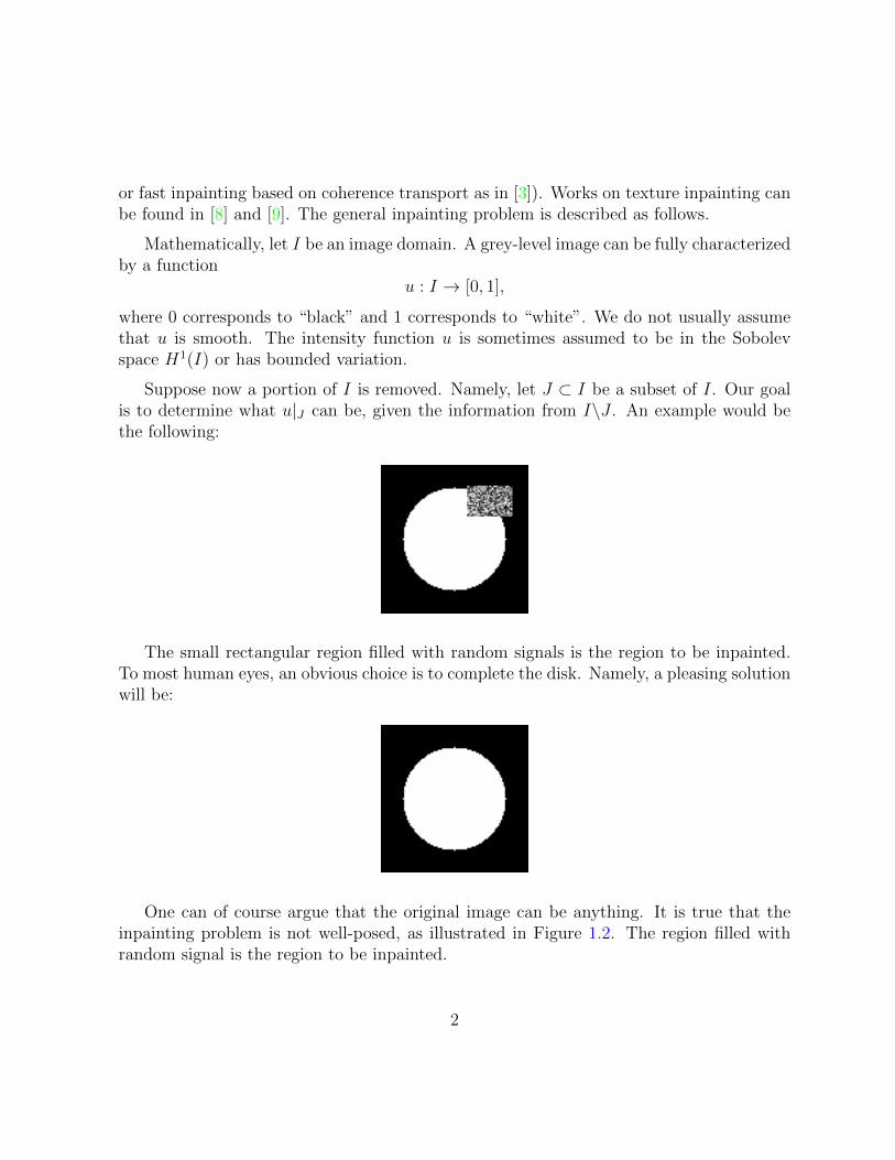
Suppose now a portion of I is removed. Namely, let J ⊂ I be a subset of I. Our goalis to determine what u|J can be, given the information from I\J . An example would bethe following:
The small rectangular region filled with random signals is the region to be inpainted.To most human eyes, an obvious choice is to complete the disk. Namely, a pleasing solutionwill be:
One can of course argue that the original image can be anything. It is true that theinpainting problem is not well-posed, as illustrated in Figure 1.2. The region filled withrandom signal is the region to be inpainted.
2
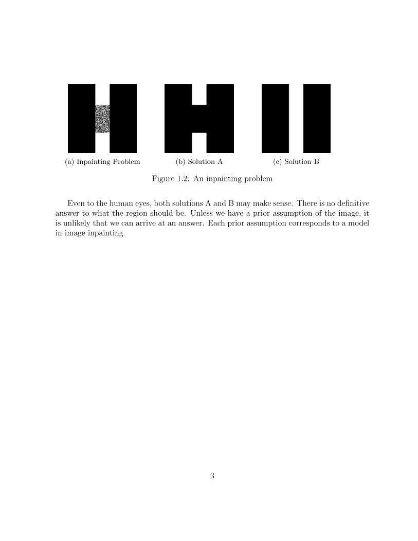
(a) Inpainting Problem (b) Solution A (c) Solution B
Figure 1.2: An inpainting problem
Even to the human eyes, both solutions A and B may make sense. There is no definitiveanswer to what the region should be. Unless we have a prior assumption of the image, itis unlikely that we can arrive at an answer. Each prior assumption corresponds to a modelin image inpainting.
3

Chapter 2
Variational Methods
There are many existing methods in image inpainting. Textbook methods involve polyno-mial interpolation or harmonic. These models work well as long as the image is resonablysmooth. But it is known that these methods are generally unable to recover edges well, be-cause these are the “reasonable” discontinuities of the image. Also, practical images oftencontain noise and blurs, which will affect the performance of these inpainting models.
To tackle these difficulties, variational partial differential equation (PDE) methods havebeen suggested.
2.1 Total Variation (TV) Inpainting
Let I be an image domain and J be a missing region. Let u0 : I → [0, 1] be the intensityfunction. The problem is to determine u|J from u0|I . Let u be a function. Following [6],and the related works [13] and [14] on image denoising, we define an energy
E(u) =
∫I
|∇u|dx+λ
2
∫I\J
(u− u0)2dx.
The first term corresponds to the total variation of u, whereas the second term is (λ2
times) the squared L2 distance of u and u0.
The total variation inpainting method seeks to find u ∈ BV (I) (i.e. all functions definedon I having bounded variations) such that E(u) is minimized. Namely, we want to find
u = argminv∈BV (I)E(v).
4
To minimize the first term in the energy roughly means that we want u to be “as smoothas possible”. In other words, we punish large variations in u. On the other hand, we alsowant to minimize the second term in the energy, which can be thought of as the distancebetween u and the original image. Including the consideration of the distance means wedo not want to be too far away from the original image in the L2 sense.
To solve for a minimizer of E(u), one approach is to derive the Euler-Lagrange equationof this functional, and solve the equation for a local minimum.
Theorem 2.1.1. Assume ∂u∂ν
= 0 on the boundary of I. The first variation of the functionalE(u) is given by
V = −∇ · ∇u|∇u|
+ λ(x)(u− u0),
where λ(x) = λ if x ∈ I\J and 0 otherwise.
Proof. With λ(x) defined above, we can write the TV functional as
E(u) =
∫I
(|∇u|+ λ(x)
2(u− u0)2)dx.
For a functional Ω(g), denote δΩ(g) = ddε
Ω(g+ε(δg))|ε=0, the first variation of Ω at g undera pertubation from g to g + δg. For two vectors v and w, denote 〈v, w〉 to be their innerproduct. Now
δE(u) =
∫I
(δ[|∇u|] +λ(x)
2δ[(u− u0)2])dx
=
∫I
(〈∇u, δ∇u〉|∇u|
+ λ(x)(u− u0)δu)dx
=
∫I
(
⟨∇u|∇u|
,∇δu⟩
+ λ(x)(u− u0)δu)dx
=
∫I
(−∇ · ∇u|∇u|
δu+ λ(x)(u− u0)δu)dx.
=
∫I
V δudx
Note that in the second last equality we have integrated by parts and used the assumptionthat ∂u
∂ν= 0.
5

Therefore, by the first optimality condition, to find local minima of the total variationfunctional, we have to solve the equation
−∇ · ∇u|∇u|
+ λ(x)(u− u0) = 0.
This is a non-linear partial differential equation and is generally hard to solve. One canconstruct and solve a linear system using a fixed point method with |∇u| delayed by oneiteration. Alternatively, starting from an initial guess u, one can use the steepest descentmethod to evolve according to the equation
∂u
∂t= ∇ · ∇u
|∇u|+ λ(x)(u0 − u).
This is equivalent to evolving u in the direction of the steepest descent of the functionalE(u), until it stops at a stationary point. This does not, however, guarantee that we reacha global minimum, although in practice the steepest descent method works fine.
Recall the problem in Figure 1.2. The inpainting region is a rectangle with verticallength L and horizontal length l. Since L > l, in the noise-free TV model (λ = ∞),solution A is preferred to solution B.
As another example, consider the disk problem in Chapter 1. A portion of the diskis covered. If we use the TV inpainting model, we will get only a triangle joining thethree extreme points on the boundary, instead of a circular disk(see Figure 2.1). This isexpected, because all the variations can possibly come from the “edge” between the blackand white regions, and hence the total variation is proportional to the length of the curvejoining these two regions. Among all such curves, the one with shortest length is a straightline. Hence, the TV model will give us a straight line instead of an arc joining these twopoints.
2.2 TV Inpainting in 3D
In three dimensions, one can formulate an equivalent inpainting problem: Given a 3D regionI where the intensity u on J ⊂ I is missing, we have to determine what the intensity u|Jcan be using information from u|I\J , under some prior assumptions. For simplicity, weassume for now that the given information is noise free. If we would like u|J to have as
6
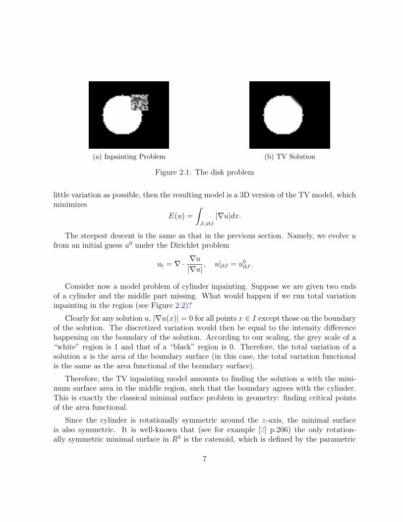
(a) Inpainting Problem (b) TV Solution
Figure 2.1: The disk problem
little variation as possible, then the resulting model is a 3D version of the TV model, whichminimizes
E(u) =
∫J∪∂J|∇u|dx.
The steepest descent is the same as that in the previous section. Namely, we evolve ufrom an initial guess u0 under the Dirichlet problem
ut = ∇ · ∇u|∇u|
, u|∂J = u0∂J .
Consider now a model problem of cylinder inpainting. Suppose we are given two endsof a cylinder and the middle part missing. What would happen if we run total variationinpainting in the region (see Figure 2.2)?
Clearly for any solution u, |∇u(x)| = 0 for all points x ∈ I except those on the boundaryof the solution. The discretized variation would then be equal to the intensity differencehappening on the boundary of the solution. According to our scaling, the grey scale of a“white” region is 1 and that of a “black” region is 0. Therefore, the total variation of asolution u is the area of the boundary surface (in this case, the total variation functionalis the same as the area functional of the boundary surface).
Therefore, the TV inpainting model amounts to finding the solution u with the mini-mum surface area in the middle region, such that the boundary agrees with the cylinder.This is exactly the classical minimal surface problem in geometry: finding critical pointsof the area functional.
Since the cylinder is rotationally symmetric around the z-axis, the minimal surfaceis also symmetric. It is well-known that (see for example [2] p.206) the only rotation-ally symmetric minimal surface in R3 is the catenoid, which is defined by the parametric
7

Figure 2.2: A cylinder with the middle part missing
equation
x = c coshv
ccosu
y = c coshv
csinu
z = v.
Figure 2.3 is a cross section of a 3D image of a catenoid (c = 0.7).
Figure 2.3: A catenoid
As seen from the figure, such a surface must inevitably be curved inwards. This means
8
that if we wanted to recover a cylinder given cylindrical boundary conditions, total variationinpainting will not be the right choice. We formulate this in the following
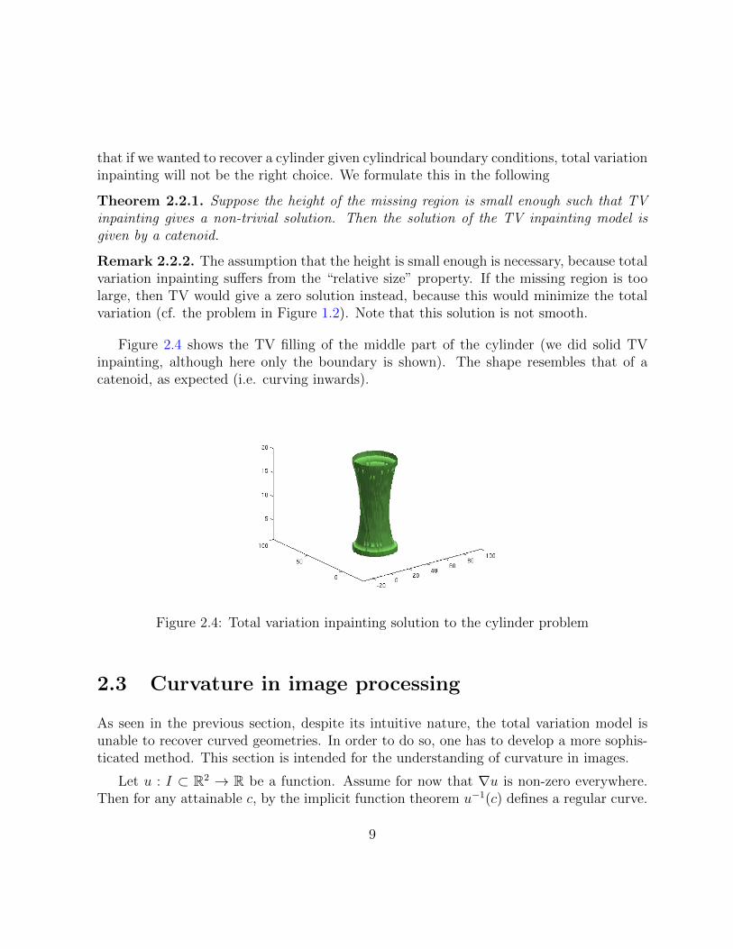
Theorem 2.2.1. Suppose the height of the missing region is small enough such that TVinpainting gives a non-trivial solution. Then the solution of the TV inpainting model isgiven by a catenoid.
Remark 2.2.2. The assumption that the height is small enough is necessary, because totalvariation inpainting suffers from the “relative size” property. If the missing region is toolarge, then TV would give a zero solution instead, because this would minimize the totalvariation (cf. the problem in Figure 1.2). Note that this solution is not smooth.
Figure 2.4 shows the TV filling of the middle part of the cylinder (we did solid TVinpainting, although here only the boundary is shown). The shape resembles that of acatenoid, as expected (i.e. curving inwards).
Figure 2.4: Total variation inpainting solution to the cylinder problem
2.3 Curvature in image processing
As seen in the previous section, despite its intuitive nature, the total variation model isunable to recover curved geometries. In order to do so, one has to develop a more sophis-ticated method. This section is intended for the understanding of curvature in images.
Let u : I ⊂ R2 → R be a function. Assume for now that ∇u is non-zero everywhere.Then for any attainable c, by the implicit function theorem u−1(c) defines a regular curve.
9

If x(t) is a parametrization of the curve, then from u(x(t)) = c we have 〈∇u, x′(t)〉 = 0. So∇u defines a normal direction. The following theorem is an elementary result in differentialgeometry, and we include it here for completeness.
Proposition 2.3.1. The curvature of the level curve u−1(c) with respect to the normaldirection ∇u is given by
κ = ∇ · ∇u|∇u|
.
In an image, at a given point, κ is the curvature of the curve through that point havingthe same grey value (isophote). An isophote can be an edge or an object, which are oftencharacterised by their grey values. Thus κ is an indicator of how curvy the isophotes of animage are. For example, straight lines have zero curvature, while a circle of radius r haveconstant positive curvature 1
r.
When κ > 0, the curve bends “away” from the normal direction |∇u|. An exampleis the circle, which always curves away from the outer normal. When κ = 0, the curveis intuitively a momentary straight line. When κ < 0, the isophote curves towards thenormal direction. Humans eyes are able to detect the sign of the curvature.
In practice, ∇u may be zero, in which case κ will be undefined. Therefore, we willconsider the following approximation of the curvature:
κε = ∇ · ∇u|∇u|+ ε
,
for some small number ε. It is clear that if κ is defined (i.e. ∇u 6= 0), then
κ = limε→0
κε.
In the numerical experiments, we will use κε as a substitute for κ.
In three dimensions, the notion of curvature is more complicated. Let S be a surfacein R3. At any point p ∈ S, among all directions you can move on the surface, there is onedirection with the maximum curvature, and one with the minimum. The sum of these twocurvatures is called the mean curvature (up to a factor of 2, depending on the convention),while the product of these two curvatures is called the Gaussian curvature.
If S is defined by an equation u(x, y, z) = c, then the mean curvature is also given by
κ = ∇ · ∇u|∇u|
,
10
which is the same formula as that of a curve in R2.
Thus, the mean curvature of a sphere in R3 of radius r is given by 2r, while that of a
cylinder with base radius r is given by 1r.
Recall that the steepest descent scheme of the total variation inpainting is given by theequation
ut = ∇ · ∇u|∇u|
.
The study by Marquina and Osher in [12] shows that a factor of |∇u| helps acceleratethe TV inpainting, and will achieve an equivalent equilibrium. Namely, the inpainting isdone by
ut = |∇u|∇ · ∇u|∇u|
= |∇u|κ
This is exactly the mean curvature motion for level sets, which is well-studied in thecontemporary Mathematical literature (one of the first significant papers on this is [10]).In other words, the total variation inpainting coincides with the mean curvature flow.
2.4 CDD Inpainting
As discussed before, using total variation inpainting, the solution to the inpainting prob-lem in Figure 2.5 is solution A, because the horizontal size of the rectangle is less thanits vertical size. TV inpainting depends highly on the relative gap size to the surroundingobjects, so in cases like that in Figure 2.5, “broken” objects may not be connected.
To solve this “problem” in TV inpainting, consider solutions A and B in terms ofisophotes (level sets). The isophotes in solution A are broken with 4 corners, while theisophotes in solution B are smooth. Since corners have large curvatures, one way to preventlarge curvatures from happening is to connect the broken bar.
In the TV model, one evolves u with the equation
ut = ∇ · ∇u|∇u|
.
11

(a) Inpainting Problem (b) Solution A (c) Solution B
Figure 2.5: The inpainting problem in Figure 1.2
We can interpret this as a diffusion process, with diffusivity equal to 1|∇u| . Following [5],
instead of 1|∇u| , we consider the new diffusion strength |κ|p
|∇u| , for p > 0. Intuitively, thediffusion is stronger when the curvature of an isophote is large, and weaker when thecurvature is small.
This gives us another inpainting scheme, known as the Curvature-Driven Diffusion(CDD) inpainting, which can connect broken objects even if the relative size requirementis not satisfied. The new scheme reads:
ut = ∇ · |κ|p∇u|∇u|
, p > 0.
Geometrically, then, TV inpainting and the CDD inpainting represent two differentphilosophies in inpainting. TV seeks to find the solution with smallest variation in intensity,while the CDD always seeks to connect broken objects. However, a problem still remains.Similar to TV inpainting, the CDD inpainting still tends to connect with straight lines(see [7] p.302). It is then desirable to have an inpainting model that can give us “curved”solutions when required. It turns out that the CDD can be incorporated into anothermodel, which can produce “curvy” isophotes.
2.5 Euler’s elastica inpainting
Instead of directly modifying the flow equation as is in CDD inpainting, another option isto modify the functional. Recall that the TV inpainting minimizes the functional
ETV (u) =
∫I
|∇u|dx+λ
2
∫I\J
(u− u0)2dx.
12

The study in [4] considered a modification of the above energy to include the curvature.Let a, b be positive constants. Define the elastica energy to be
E(u) =
∫I
(a+ bκ2)|∇u|dx+λ
2
∫I\J
(u− u0)2dx,
where κ = ∇ · ∇u|∇u| is the (mean) curvature of level sets of u.
Equivalently, assuming the given part of the image is noise-free (i.e. we will not changethat part), we can work with
E(u) =
∫I
(a+ bκ2)|∇u|dx.
The a-part of the energy corresponds to that of the total variation, while the b-partof the energy corresponds to minimizing the curvature of the isophotes. Large curvatureswill be punished, as in the CDD model.
Define λ(x) = λ if x ∈ I\J and 0 otherwise. The steepest descent equation of theenergy E(u) is
ut = ∇ · V − λ(x)(u− u0),
where
V = (a+ bκ2)n− P (1
|∇u|∇(2bκ|∇u|)),
n =∇u|∇u|
,
P (x) = x− 〈x,n〉n.
With this functional, the inpainting model tries to extend isophotes into the inpaintingdomain by Euler’s elasticas, which are known as stationary curves of the energy
E1(γ) =
∫γ
(a+ bκ2)ds,
where ds denotes the arc length element. Euler’s elasticas are smooth and can have cur-vatures (controlled by the magnitude of b). In contrast, the stationary curves of
E2(γ) =
∫γ
ds = length(γ)
13
are clearly linear. This explains why TV inpainting, in general, favours connection bystraight lines. The change from the TV energy to the elastica energy effectively coorespondsto the change of our prior model of curves. In the TV model the isophotes are modelledby straight lines while in the elastica inpainting the isophotes are modelled by Euler’selasticas. Thus, if “curvy” solutions are required the elastica inpainting would be a moreappropriate choice.
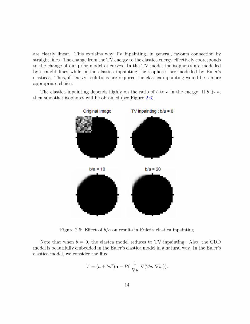
The elastica inpainting depends highly on the ratio of b to a in the energy. If b a,then smoother isophotes will be obtained (see Figure 2.6).
Figure 2.6: Effect of b/a on results in Euler’s elastica inpainting
Note that when b = 0, the elastca model reduces to TV inpainting. Also, the CDDmodel is beautifully embedded in the Euler’s elastica model in a natural way. In the Euler’selastica model, we consider the flux
V = (a+ bκ2)n− P (1
|∇u|∇(2bκ|∇u|)).
14

We can write V = Vn + Vt, where
Vn = (a+ bκ2)n,
Vt = −P (1
|∇u|∇(2bκ|∇u|))
are respectively the normal part and tangential part of V . The normal divergence is equalto
∇ · Vn = ∇ · (a+ bκ2
|∇u|∇u)
since n = ∇u|∇u| , which is similar to the flow equation in the CDD model:
ut = ∇ · |κ|p∇u|∇u|
, p > 0.
Therefore, if b a, properties of CDD (i.e. ability to connect) will become moreapparent, as demonstrated in the Figure 2.7.
Figure 2.7: Effect of b/a on connectivity in Euler’s elastica inpainting.
15

2.6 Euler’s elastica inpainting in 3D
Now we return to the cylinder problem in Figure 2.2. An elementary result in classicaldifferential geometry states that a minimal surface has zero mean curvature. In our context,this corresponds to κ = 0, analytically in the interior region.
A TV solution does not only (locally) minimize the variation. When analytic equilib-rium is achieved, the steady state satisfies
∇ · ∇u|∇u|
= 0,
i.e. κ = 0. Recall that the Euler’s elastica model seeks to minimize
E(u) =
∫I
(a+ bκ2)|∇u|dx.
When the first term is already a local minimum and the second term is mostly zero inthe interior, there is no reason to believe that a cylinder can be recovered by the Euler’selastica method when generalized, that is, with the same formula of κ (see Figure 2.8).
Figure 2.8: Euler’s elastica solution of the cylinder problem
16

Chapter 3
Minimal Curvature Variation Flow(MCVF)
3.1 The functional
Inspired by [16], the motivation of the model is originally based on the lack of sensitivityof the total variation model to the digital curvature of the image. In order to have curvedgeometries, one has to take into account the curvature. The elastica inpainting is a goodchoice in this aspect.
As described before, the presence of the curvature in Euler’s elastica functional seeks topunish large curvatures. Thus, smoother isophotes can be obtained. However, there is noapparent reason why we have to minimize the curvature whenever possible. It is true thatthis permits smoother isophotes, but the problem associated with this becomes apparentwhen we consider its direct generalization in three dimensions. A minimization of the(mean) curvature will distort the cylinder. One solution to this is to consider preservingthe curvature, instead of minimizing it.
In this model, we want to minimize the change of curvature in the inpainting area alongevery level curve (or within any level area) of the intensity function.
Let I be the image domain, and u : I → [0, 1] be the intensity function. Then thedigital curvature of u is defined by
κ = ∇ · ∇u|∇u|
.
17

For now, let us first assume that u is regular, i.e. ∇u is never 0. Then κ exists and isdefined everywhere on I. By the implicit function theorem, the equation u(x) = c definesa regular curve for every attainable c. On any such level curve, its curvature is given by κ.
Now we consider the functional
Φ(u) =
∫ 1
0
∫u(x,y)=c
|∇κ|2dsdc,
where ds denotes the arc-length integral, and dc denotes the differential element acrosslevel sets, i.e. the cotangent dual to ∇u. This is the total change of curvature (square L2
norm) on level sets.
On any level curve u(x, y) = c, by the assumption that |∇u| 6= 0 and the inverse functiontheorem, we have a unique anti-clockwise vector field e1 satisfying |e1| = 1. Depending onthe convention, the normal vector can be written as ± ∇u|∇u| . Denote e2 = ∇u
|∇u| .
Clearly e1 and e2 form an orthonormal basis at each point they are defined, so theirduals e1 and e2 satisfy e1∧e2 = dx∧dy, where ∧ is the wedge product of differential forms.
Since |e1| = 1, we have that e1 = ds. Similarly dc = |∇u|e2. Therefore, we can simplifythe functional as follows:
Φ(u) =
∫ 1
0
∫u(x,y)=c
|∇κ|2dsdc
=
∫ 1
0
∫u=c
|∇κ|2|∇u|e1 ∧ e2
=
∫ ∫|∇κ|2|∇u|dxdy
This is the energy we consider in this study. In other words, we seek inpainting solutionsthat minimize (at least locally)
Φ(u) =
∫ ∫|∇κ|2|∇u|dxdy.
This has the property that it punishes large variation of the digital curvature alonglevel sets.
Suppose the inpainting domain contains a curved isophote, as in Figure 2.1. Thecurvature of a circle is 1
R, where R is the radius. If we want to minimize the change of
18

curvature, a global minimum of the function will be given by the exact disk. We will showin section 3.4 that a disk can be well recovered by the MCVF.
The same idea applies to three dimensional inpainting. The cylinder has a constantmean curvature of 1
R. The direct generalization of Euler’s elastica will not preserve this,
while the MCVF respects the mean curvature in this case. This claim will also be confirmedin section 3.6.
3.2 Derivation of the Euler-Lagrange equation
In this section we will work with the Euler-Lagrange equation of the aforementioned func-tional.Let J ⊂ I be the inpainting region.
Theorem 3.2.1. Assume ∇κ = ∇(∇ · (|∇u|∇κ)) = 0 on the boundary of J . Then thefirst variation of the functional Φ is given by −∇ · V , where
V =2
|∇u|P (∇(∇ · (|∇u|∇κ))) + |∇κ|2n,
P (x) = x− 〈x,n〉n,
n =∇u|∇u|
.
Proof. For a functional Ψ(u) and a given u0, denote
δΨ(u0) :=∂
∂tΨ(u0 + tδu)|t=0,
which is the first variation at u0 under the perturbation from u0 to u0 + δu.We also denote by 〈f〉 =
∫f , following the notation in [4]. Now for the functional
Φ(u) =
∫ ∫|∇κ|2|∇u|dxdy,
we have
δΦ(u) =⟨δ(|∇κ|2|∇u|)
⟩=
⟨δ(|∇κ|2)|∇u|
⟩+⟨|∇κ|2δ|∇u|
⟩= 〈2 〈∇κ, δ∇κ〉 |∇u|〉+
⟨|∇κ|2δ|∇u|
⟩= 〈2 〈|∇u|∇κ,∇δκ〉〉+
⟨|∇κ|2δ|∇u|
⟩= −2 〈∇ · (|∇u|∇κ)δκ〉+
⟨|∇κ|2δ|∇u|
⟩,
19

where the last line follows from the integration by parts, and the assumption that ∇κ = 0along the boundary.
Now we compute δκ:
δκ = δ(∇ · ∇u|∇u|
)
= ∇ · ( 1
|∇u|δ(∇u) +∇u(δ(
1
|∇u|)))
= ∇ · ( 1
|∇u|∇(δu)− 〈∇u, δ(∇u)〉
|∇u|3∇u)
= ∇ · ( 1
|∇u|∇(δu)− 〈∇u,∇(δu)〉
|∇u|3∇u)
= ∇ · ( 1
|∇u|P (∇(δu))) = ∇ · ( 1
|∇u|P (∇(δu))),
where P is the projection onto the tangential component defined before, and if we writen = ∇u
|∇u| , it can be rewritten as
x =〈x,∇u〉|∇u|2
∇u+ Px.
Thus the tangential part is
δκ = ∇ · ( 1
|∇u|P (∇(δu))). (3.1)
Next we have that
δ|∇u| = 〈∇u,∇δu〉|∇u|
= 〈n,∇δu〉 , (3.2)
where n = ∇u|∇u| .
20

With (3.1), (3.2) and applying integration by parts successively, we get
δΦ(u) = −2 〈∇ · (|∇u|∇κ)δκ〉+⟨|∇κ|2δ|∇u|
⟩= −2
⟨∇ · (|∇u|∇κ)∇ · ( 1
|∇u|P (∇(δu)))
⟩+⟨|∇κ|2 〈n,∇δu〉
⟩= 2
⟨⟨∇(∇ · (|∇u|∇κ)),
1
|∇u|P (∇(δu))
⟩⟩−⟨∇ · (|∇κ|2n)δu
⟩= 2
⟨⟨1
|∇u|P (∇(∇ · (|∇u|∇κ))),∇(δu)
⟩⟩−⟨∇ · (|∇κ|2n)δu
⟩= −2
⟨∇ · ( 1
|∇u|P (∇(∇ · (|∇u|∇κ))))δu
⟩−⟨∇ · (|∇κ|2n)δu
⟩= 〈−(∇ · V )δu〉 ,
where we defined
V =2
|∇u|P (∇(∇ · (|∇u|∇κ))) + |∇κ|2n.
Notice that we have further used the assumptions that
∇(∇ · (|∇u|∇κ)) = ∇κ = 0
on the boundary.
Remark 3.2.2. For regularity, we will sometimes add a TV-regularizing term to thefunctional. The combined functional is
Φ(u) =
∫ ∫(a+ b|∇κ|2)|∇u|dxdy,
where ba
is large. The resulting steepest descent equation is
∂u
∂t= aκ+ b∇ · V,
where V is as described in Theorem 3.2.1.
3.3 Numerical Methods
In this section we present our discretization for ∇ · V , where
V =2
|∇u|P (∇(∇ · (|∇u|∇κ))) + |∇κ|2n.
21
We compute the curvature in a way suggested in [14]. Let v be a function, and h, k bethe spatial step sizes of the x and y directions, respectively. Denote D+
i v to be the forwardfinite difference of v in coordinate i, and D−j v to be the backward finite difference of v incoordinate j. Let
mi = minmod(D+i u,D
−i u),
for i = 1, 2, where
minmod(a, b) = (sgn a+ sgn b
2) min(|a|, |b|).
The curvature κ = ∇ · ∇u|∇u| is computed using
κi,j ≈ D−x (D+x u
D+x u+m2
2
)i,j +D−y (D+y u
D+y u+m2
1
)i,j.
Next we have to compute ∇ · (|∇u|∇κ). This is done using a half-point discretization.Denote g = ∇u. We approximate
gi+ 12,j ≈
gi+1,j + gi,j2
.
Similarly, gi− 12,j and gi,j± 1
2are done by averaging. We also have to specify half-points for
∇κ:
(κx)i+ 12,j =
κi+1,j − κi,jh
Similarly we can evaluate (κx)i− 12,j, and (κy)i,j± 1
2. Then we use the following discretiza-
tion for ∇ · (|∇u|∇κ):
∇ · (|∇u|∇κ)i,j ≈(gi+ 1
2,j(κx)i+ 1
2,j − gi− 1
2,j(κx)i− 1
2,j)
h+
(gi,j+ 12(κx)i,j+ 1
2− gi,j− 1
2(κx)i,j− 1
2)
k.
Before we proceed, we need to work out a more explicit formula for V . In two dimen-sions, since P is the projection onto the tangent direction, we can write
P (x) = 〈x, t〉 t,
where t = (−uy ,ux)|∇u| . Denote r = ∇ · (|∇u|∇κ), which we computed above. Now we have
V =2
|∇u|P (∇(∇ · (|∇u|∇κ))) + |∇κ|2n
=2
|∇u|〈∇r, t〉 t + |∇κ|2n.
22

Denote s = 〈∇r, t〉. Then
V 1 =2s
gt1 + |∇κ|2n1
=2s
g2(−uy) +
|∇κ|2uxg
,
V 2 =2s
gt2 + |∇κ|2n2
=2s
g2(ux) +
|∇κ|2uyg
.
Finally we compute ∇ · V using half-point discretizations again. Namely,
∇ · Vi,j ≈V 1i+ 1
2,j− V 1
i− 12,j
h+V 2i,j+ 1
2
− V 1i,j− 1
2
k.
The half-points of g and |∇κ|2 are done by averaging as in the above approximation ofgi± 1
2,j and gi,j± 1
2. Then we have to approximate half-points of ux, uy and s.
Again, let v be some function. Suppose we want to approximate (vx)i+ 12,j. Then we
can use
(vx)i+ 12,j ≈
vi+1,j − vi,jh
.
Similarly we can approximate (vx)i− 12,j. For (vx)i,j+ 1
2, we shall use
(vx)i,j+ 12≈ average(
vi+1,j+1 − vi−1,j+1
2h,vi+1,j − vi−1,j
2h).
On the other hand, it was suggested in [4] that using the following minmod approximationpreserves edges better:
(vx)i,j+ 12≈ minmod(
vi+1,j+1 − vi−1,j+1
2h,vi+1,j − vi−1,j
2h).
Now we return to the half-point values of ux, uy and s. The half-points values of ux, uycan be approximated using the method mentioned above. Note that
s = 〈∇r, t〉 = rx(−uy) + ryux,
which are combinations of derivatives. The half-point values of each derivative is thenapproximated the same way as outlined above. This finishes the discretization of ∇ · V .
23

3.4 Numerical Results in images
For the disk problem in Figure 2.1, unlike the total variation solution in Figure 3.1, ourproposed algorithm is able to produce a curved result.
(a) Disk Inpainting Problem (b) MCVF Solution
Figure 3.1: The disk problem and the MCVF solution
This is because the boundary of the disk (a circle) has non-zero curvature, whereasa straight line always has curvature 0. To connect with minimal change in curvature inisophotes, a non-zero curvature connection is preferred.
On the other hand, if we work with straight isophotes as in total variation inpainting,our inpainting algorithm will give a straight connection.
(a) Edge Inpainting Problem (b) MCVF Solution
Figure 3.2: Straight edge inpainting problem and the MCVF solution
Our algorithm does a very good job in restoring general images. Figure 3.3 shows animage with four bars removed, and its restoration with the MCVF. The resulting image
24
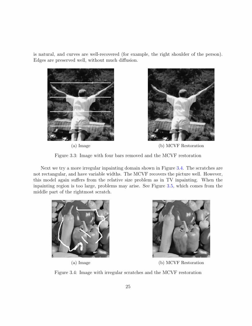
is natural, and curves are well-recovered (for example, the right shoulder of the person).Edges are preserved well, without much diffusion.
(a) Image (b) MCVF Restoration
Figure 3.3: Image with four bars removed and the MCVF restoration
Next we try a more irregular inpainting domain shown in Figure 3.4. The scratches arenot rectangular, and have variable widths. The MCVF recovers the picture well. However,this model again suffers from the relative size problem as in TV inpainting. When theinpainting region is too large, problems may arise. See Figure 3.5, which comes from themiddle part of the rightmost scratch.
(a) Image (b) MCVF Restoration
Figure 3.4: Image with irregular scratches and the MCVF restoration
25

Figure 3.5: Unnatural connection between two vegetables
As a classic example, in Figure 3.6 we show the results of the MCVF in text removal.The algorithm recovers the picture well. Sharp edges are well preserved, and the sensitivityto the change of “environment” is good.
(a) Image (b) MCVF Restoration
Figure 3.6: Image with text and the MCVF restoration
Despite the capability of the model to restore general images, the following exampleshows that the MCVF does not connect broken edges as well as the CDD (see Figure 3.7).The “relative size” problem reappears, although we can see that if the inpainting domainis not too large, the reconstruction of a curved arc is good (see Figure 3.8).
26

(a) Arc Inpainting Problem (b) MCVF Solution
Figure 3.7: Arc(thin) inpainting problem and the MCVF solution
(a) Arc Inpainting Problem (b) MCVF Solution
Figure 3.8: Arc(thick) inpainting problem and the MCVF solution
3.5 Applications to noise removal
As a bonus application, with a little modification the MCVF can be applied in imagedenoising. Although this is not our main focus, the result is satisfactory.
Using the same idea of total variation denoising, we add a distance term to the func-tional. Suppose that
u0 : I → [0, 1]
is some noisy image. We consider minimizing the functional
Φ(u) =
∫ ∫|κ|2|∇u|dxdy +
λ
2
∫ ∫|u− u0|2dxdy.
Namely, we want to find the closest image to u0 in L2 that minimizes the curvaturevariation at the same time. Using the same argument as in Theorem 3.2.1, we can show
27

that the steepest descent equation is
∂u
∂t= ∇ · V + λ(u0 − u),
where
V =2
|∇u|P (∇(∇ · (|∇u|∇κ))) + |∇κ|2n,
P (x) = x− 〈x,n〉n,
n =∇u|∇u|
.
In the experiments, we used the same discretizations as described above.
In Figure 3.9(b), we have added 10 % salt and pepper noise to the image in Figure3.9(a). The MCVF restoration, shown in 3.9(c), recovers the image very well. Edges,curved or straight, are preserved well with little or no diffusion.
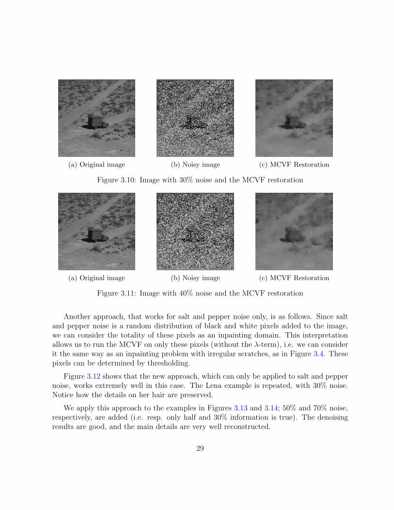
In Figure 3.10 and Figure 3.11, more noise has been added to Figure 3.10(a) and 3.11(a).The image in Figure 3.10 was polluted with 30% salt and pepper noise, while that in Figure3.11 was polluted with 40%. It is clear that the MCVF is able to identify and preserve therobust information from these amounts of noise.
(a) Original image (b) Noisy image (c) MCVF Restoration
Figure 3.9: “Lena” with 10% noise and the MCVF restoration
28
(a) Original image (b) Noisy image (c) MCVF Restoration
Figure 3.10: Image with 30% noise and the MCVF restoration
(a) Original image (b) Noisy image (c) MCVF Restoration
Figure 3.11: Image with 40% noise and the MCVF restoration
Another approach, that works for salt and pepper noise only, is as follows. Since saltand pepper noise is a random distribution of black and white pixels added to the image,we can consider the totality of these pixels as an inpainting domain. This interpretationallows us to run the MCVF on only these pixels (without the λ-term), i.e. we can considerit the same way as an inpainting problem with irregular scratches, as in Figure 3.4. Thesepixels can be determined by thresholding.
Figure 3.12 shows that the new approach, which can only be applied to salt and peppernoise, works extremely well in this case. The Lena example is repeated, with 30% noise.Notice how the details on her hair are preserved.
We apply this approach to the examples in Figures 3.13 and 3.14; 50% and 70% noise,respectively, are added (i.e. resp. only half and 30% information is true). The denoisingresults are good, and the main details are very well reconstructed.
29

(a) Original image (b) Noisy image (c) MCVF Restoration
Figure 3.12: “Lena” with 30% noise and the MCVF restoration
(a) Original image (b) Noisy image (c) MCVF Restoration
Figure 3.13: “Elaine” with 50% noise and the MCVF restoration
(a) Original image (b) Noisy image (c) MCVF Restoration
Figure 3.14: “Elaine” with 70% noise and the MCVF restoration
30

3.6 Numerical Results in 3D
In three dimensions, unlike the total variation inpainting, the MCVF is able to restore thecylinder without curving inwards. This is because the cylinder has a non-zero (mean) cur-vature equal to 1/r, where r is the radius of the base circle. The total variation inpainting,while aiming to achieve the smallest intensity variation possible, ignores the curvature.The result is as in Figure 2.4.
It was also studied in Section 2.6 that a direct generalization of the Euler’s elasticainpainting method also gives a distorted cylinder in the cylinder problem (see Figure 2.8).This is because both total variation inpainting and the elastica inpainting try to minimize(through the b-term) the mean curvature of the level sets.
However, since the MCVF considers the change in (mean) curvature along isophotes,the shrinking is not preferred because this model favours little variation in the curvature.Thus, in terms of restoring a cylinder, the MCVF is a better choice (see Figure 3.15). Notewe were restoring a solid cylinder, although only the boundary of our inpainting result isshown.
In Figure 3.16, our given image is a solid torus (doughnut) with a section removed (theboundary is shown in the pictures). The MCVF solution is shown in Figure 3.17. Thisexample demonstrates two properties of the MCVF:1.“Curved” boundary surface is successfully restored.2. Provided the gap size is not too large, the MCVF is able to connect solid objects, withdisconnected parts matched correctly.
When the gap size is large, this model, as in most PDE inpainting methods, fails toconnect the disconnected parts.
Finally we present a slightly different formulation of the 3D inpainting problem. Westart with an initial image and a final image in an image sequence, and use the inpaintingtechnique to fill out the middle slices. This is presented in Figure 3.18.
31
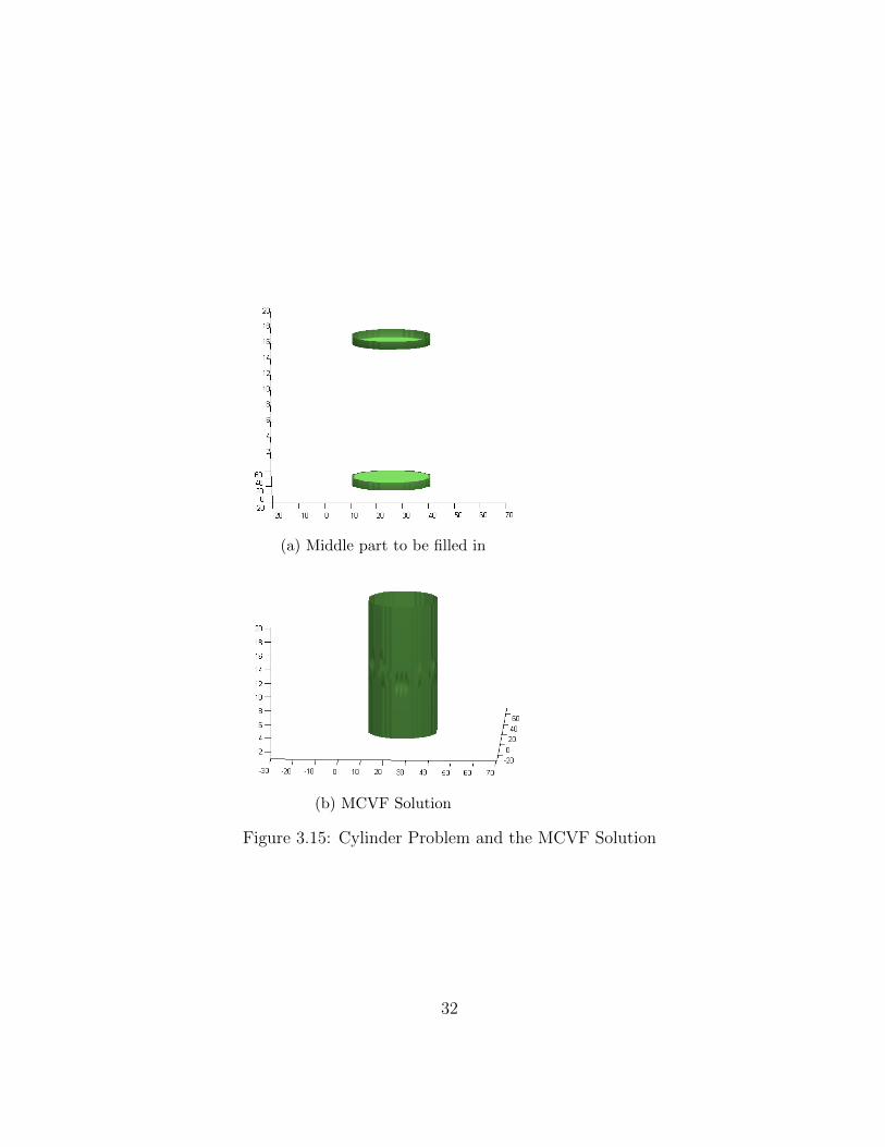
(a) Middle part to be filled in
(b) MCVF Solution
Figure 3.15: Cylinder Problem and the MCVF Solution
32
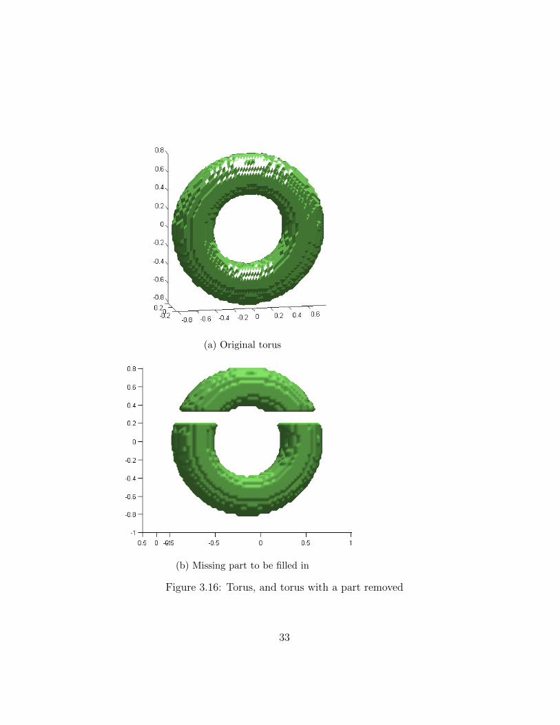
(a) Original torus
(b) Missing part to be filled in
Figure 3.16: Torus, and torus with a part removed
33

(a) MCVF Restoration, angle 1
(b) MCVF Restoration, angle 2
Figure 3.17: MCVF filling of the missing part in Figure 3.16
34
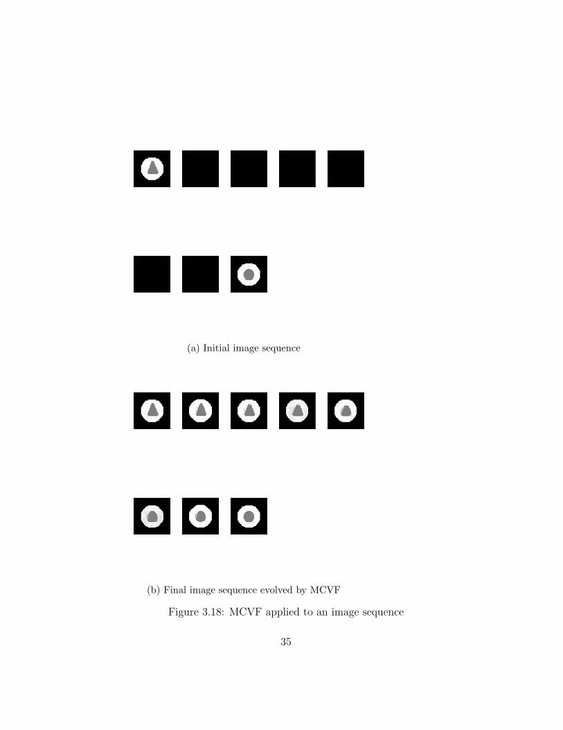
(a) Initial image sequence
(b) Final image sequence evolved by MCVF
Figure 3.18: MCVF applied to an image sequence
35

Chapter 4
Summary
In the previous chapters we have reviewed the general ideas in variational inpainting meth-ods. In particular, the total variation inpainting model and the Euler’s elastica model havebeen studied in detail. These two models behave differently, which is a result of the differ-ent prior assumptions of the isophotes (the TV inpainting tries to complete the isophotesby straight lines, while the Euler’s elastica method tries to do so through elasticas). The3D generalizations of these methods have been studied, and we have found that thesemethods fail to recover a solid cylinder, which is one of the simplest, yet most important,examples in 3D inpainting.
We have then proposed a new model (MCVF), which seeks to minimize the change ofcurvature along isophotes. As shown in the numerical results, our new model does notonly do well in general image inpainting, but also in three dimensions. The MCVF is ableto recover a cylinder well, and produces nice results in other 3D inpainting problems, asshown in the examples in Section 3.6.
While the MCVF works well in these situations, we have found that the relative sizeproblem, which is commonly found in PDE inpainting methods, remains in our new model.Information fails to propagate far across a big gap, as illustrated in Figure 3.7. In addition,due to the presence of high order spatial derivatives in the steepest descent equation, thesize of time steps 4t must be very small in order to guarantee numerical stability. Forlarge images, the time marching is slow.
Further research includes improving the connectivity of the model (i.e. to lessen theeffect of the relative size) and developing a fast implementation of the algorithm.
36
References
[1] Marcelo Bertalmio and Guillermo Sapiro. Image inpainting. In Computer Graphics(SIGGRAPH 2000), pages 417–424, 2000.
[2] P.A. Blaga. Lectures on the Differential Geometry of Curves and Surfaces. NapocaPressr, Cluj-Napoca, Romania, 2005.
[3] Folkmar Bornemann and Tom Marz. Fast image inpainting based on coherence trans-port. J. Math. Imaging Vis., 28(3):259–278, July 2007.
[4] Tony F. Chan, Sung Ha Kang, and Jianhong Shen. Euler’s elastica and curvature-based inpainting. SIAM J. Appl. Math., 63(2):564–592 (electronic), 2002.
[5] Tony F. Chan and Jianhong Shen. Non-texture inpainting by curvature-driven diffu-sions (cdd). J. Visual Comm. Image Rep, 12:436–449, 2001.
[6] Tony F. Chan and Jianhong Shen. Mathematical models for local nontexture inpaint-ings. SIAM J. Appl. Math., 62(3):1019–1043 (electronic), 2001/02.
[7] Tony F. Chan and Jianhong Shen. Image processing and analysis. Society for Industrialand Applied Mathematics (SIAM), Philadelphia, PA, 2005. Variational, PDE, wavelet,and stochastic methods.
[8] Alexei Efros, , Alexei A. Efros, and Thomas K. Leung. Texture synthesis by non-parametric sampling. In In International Conference on Computer Vision, pages1033–1038, 1999.
[9] M. Elad, J.-L. Starck, P. Querre, and D. L. Donoho. Simultaneous cartoon andtexture image inpainting using morphological component analysis (MCA). Appliedand Computational Harmonic Analysis, 19:340–358, 2005.
37

[10] Gerhard Huisken. Flow by mean curvature of convex surfaces into spheres. J. Differ-ential Geom., 20(1):237–266, 1984.
[11] J. Jost. Riemannian Geometry and Geometric Analysis. Springer, United States, fifthedition, 2008.
[12] Antonio Marquina and Stanley Osher. Explicit algorithms for a new time dependentmodel based on level set motion for nonlinear deblurring and noise removal. SIAM J.Sci. Comput., 22(2):387–405 (electronic), 2000.
[13] Leonid I. Rudin and Stanley Osher. Total variation based image restoration with freelocal constraints. Proc. 1st IEEE ICIP., 1:31–35, 1994.
[14] Leonid I. Rudin, Stanley Osher, and Emad Fatemi. Nonlinear total variation basednoise removal algorithms. Phys. D, 60(1-4):259–268, November 1992.
[15] V. V. Voronin, V. I. Marchuk, A. I. Sherstobitov, and K. O. Egiazarian. Imageinpainting using cubic spline-based edge reconstruction. In Proceedings of the SPIE,volume 8295, 2012.
[16] Guoliang Xu and Qin Zhang. Minimal mean-curvature-variation surfaces and theirapplications in surface modeling. GMP 2006, Lecture Notes in Computer Sciences,4077:357–370, 2006.
38