ming-feng yeh1 chapter 7 supervisedhebbianlearning
TRANSCRIPT

Ming-Feng Yeh 1
CHAPTER 7CHAPTER 7
SupervisedSupervisedHebbianHebbianLearningLearning

Ming-Feng Yeh 2
ObjectivesObjectives
The Hebb rule, proposed by Donald Hebb in 1949, was one of the first neural network learning laws. A possible mechanism for synaptic modification in the brain.Use the linear algebra concepts to explain why Hebbian learning works.The Hebb rule can be used to train neural networks for pattern recognition.

Ming-Feng Yeh 3
Hebb’s PostulateHebb’s Postulate
Hebbian learning (The Organization of Behavior)When an axon of cell A is near enough to excite a cell
B and repeatedly or persistently takes part in firing it; some growth process or metabolic change takes place in one or both cells such that A’s efficiency, as one of the cells firing B, is increased.
當細胞 A 的軸突到細胞 B 的距離進到足夠刺激它,且反覆或持續地刺激 B ,則在這兩個細胞或其中一個將會發生某種成長過程或代謝反應,以增加 A 對 B 的刺激效果。

Ming-Feng Yeh 4
Linear AssociatorLinear Associator
W
SR
R
p
R1
a
S1
n
S1
S
a = Wp
Q
jjiji pwa
1
The linear associator is an example of a type of neuralnetwork called an associator memory.
The task of an associator is to learn Q pairs ofprototype input/output vectors: {p1,t1}, {p2,t2},…, {pQ,tQ}.
If p = pq, then a = tq. q = 1,2,…,Q.If p = pq + , then a = tq + .

Ming-Feng Yeh 5
Hebb Learning RuleHebb Learning RuleIf two neurons on either side of a synapse are activated simultaneously, the strength of the synapse will increase.
The connection (synapse) between input pj and output ai is the weight wij.
Unsupervised learning rule
jqiqoldij
newijjqjiqi
oldij
newij pawwpgafww )()(
)1( T qqoldnew
jqiqoldij
newij ptww ptWW
Supervised learning rule
Not only do we increase the weight when pj and ai are positive, but we also increase the weight when they are both negative.

Ming-Feng Yeh 6
Supervised Hebb RuleSupervised Hebb RuleAssume that the weight matrix is initialized to zero and each of the Q input/output pairs are applied once to the supervised Hebb rule. (Batch operation)
T
T
T2
T1
21
1
TTT22
T11
TP
p
p
p
ttt
ptptptptW
Q
Q
Q
qqqQQ
QQ pppPtttT 2121 , where
Ming-Feng Yeh 7
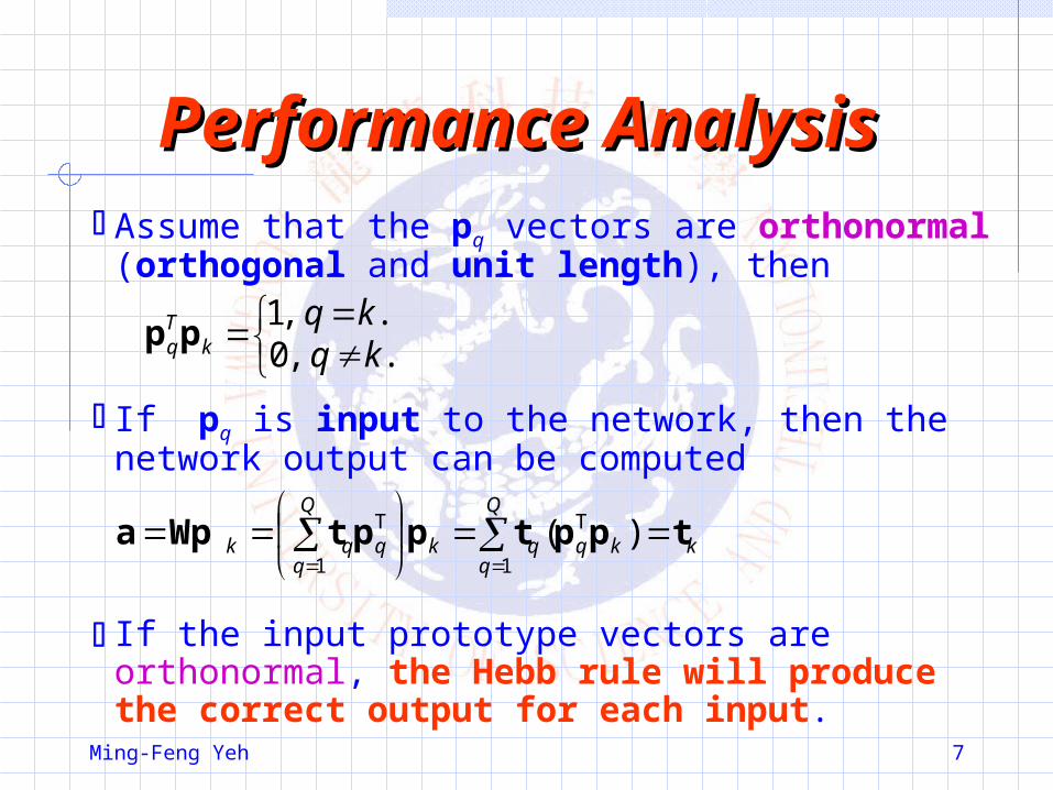
Performance AnalysisPerformance AnalysisAssume that the pq vectors are orthonormal (orthogonal and unit length), then
. ,0. ,1
kqkq
kTqpp
If pq is input to the network, then the network output can be computed
k
Q
qkqqk
Q
qqqk tpptpptWpa
1
T
1
T )(
If the input prototype vectors are orthonormal, the Hebb rule will produce the correct output for each input.

Ming-Feng Yeh 8
Performance AnalysisPerformance AnalysisAssume that each pq vector is unit length, but they are not orthogonal. Then
k
Q
qkqqk tpptWpa
1
T )( kq
kqq )( Tppterro
r
The magnitude of the error will depend on the amount of correlation between the prototype input patterns.

Ming-Feng Yeh 9
Orthonormal CaseOrthonormal Case
1
1,
5.0
5.0
5.0
5.0
,1
1,
5.0
5.0
5.0
5.0
2211 tptp
0110
10015.05.05.05.0
5.05.05.05.0
11
11TTPW
.1
1 ,
1
121
WpWp Success!!

Ming-Feng Yeh 10
Not Orthogonal CaseNot Orthogonal Case
1,
5774.0
5774.0
5774.0
,1,
5774.0
5774.0
5774.0
2211 tptp
0547.10
5774.05774.05774.0
5774.05774.05774.011T
TPW
.8932.0 ,8932.0 21 WpWp
The outputs are close, but do not quite match the target outputs.

Ming-Feng Yeh 11
Solved Problem P7.2Solved Problem P7.2
21 ppTP
:1p :2p T1 111111 p
T2 111111 p
i. 02T1 pp Orthogonal, not orthonormal, 62
T21
T1 pppp
202020
020202
202020
020202
202020
020202
TTPWii.

Ming-Feng Yeh 12
Solutions of Problem P7.2Solutions of Problem P7.2
iii. :tp T111111 tp
2
1
1
1
1
1
1
6-
2
6
2
6
2-
hardlims)(hardlims pWpa
t
:1p :2pHamming dist. = 2 Hamming dist. = 1
Ming-Feng Yeh 13
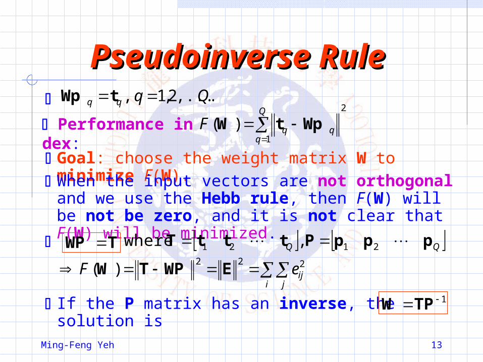
Pseudoinverse RulePseudoinverse Rule.,...,2,1 , Qqqq tWp
Performance index:
2
1
)(
Q
qqqF WptW
Goal: choose the weight matrix W to minimize F(W).When the input vectors are not orthogonal and we use the Hebb rule, then F(W) will be not be zero, and it is not clear that F(W) will be minimized.
TWP
i j
ijeF 222)( EWPTW
If the P matrix has an inverse, the solution is 1TPW
QQ pppPtttT 2121 , where

Ming-Feng Yeh 14
Pseudoinverse RulePseudoinverse RuleP matrix has an inverse iff P must be a square matrix. Normally the pq vectors (the column of P) will be independent, but R (the dimension of pq, no. of rows) will be larger than Q (the number of pq vectors, no. of columns). P does not exist any inverse matrix.
The weight matrix W that minimizes the performance
index is given by the
pseudoinverse rule .
2
1
)(
Q
qqqF WptW
TPW
where P+ is the Moore-Penrose pseudoinverse.
Ming-Feng Yeh 15
Moore-Penrose Moore-Penrose PseudoinversePseudoinverse
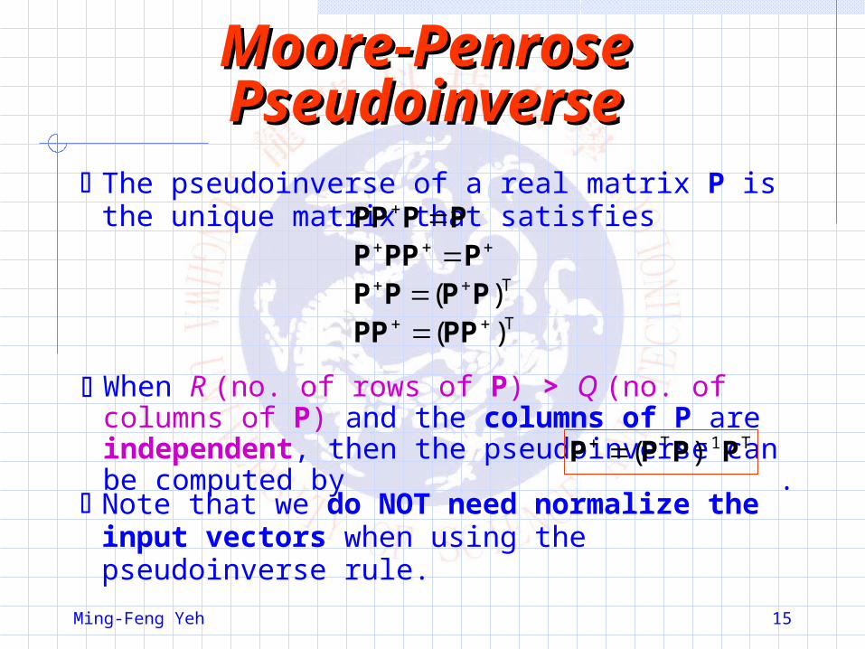
The pseudoinverse of a real matrix P is the unique matrix that satisfies
T
T
)()(
PPPPPPPP
PPPPPPPP
When R (no. of rows of P) > Q (no. of columns of P) and the columns of P are independent, then the pseudoinverse can be computed by .
T1T )( PPPP
Note that we do NOT need normalize the input vectors when using the pseudoinverse rule.

Ming-Feng Yeh 16
Example of Example of Pseudoinverse RulePseudoinverse Rule
1,
1
1
1
,1,
1
1
1
2211 tptp
111
111TP
25.05.025.0
25.05.025.0
111
111
31
13)(
T
T1T PPPP
01025.05.025.0
25.05.025.011
TPW
2211 1
1
1
1
010 ,1
1
1
1
010 tWptWp

Ming-Feng Yeh 17
Autoassociative MemoryAutoassociative MemoryThe linear associator using the Hebb rule is a type of associative memory ( tq pq ). In an autoassociative memory the desired output vector is equal to the input vector ( tq = pq ).
An autoassociative memory can be used to store a set of patterns and then to recall these patterns, even when corrupted patterns are provided as input.
11, tp 22 , tp 33 , tp W
3030
30
p
301
a30
1
n
301
30T33
T22
T11 ppppppW

Ming-Feng Yeh 18
Corrupted & Noisy VersionsCorrupted & Noisy VersionsRecovery of 50% Occluded Patterns
Recovery of Noisy Patterns
Recovery of 67% Occluded Patterns

Ming-Feng Yeh 19
Variations ofVariations ofHebbian LearningHebbian Learning
Many of the learning rules have some relationship to the Hebb rule.
The weight matrices of Hebb rule have very large elements if there are many prototype patterns in the training set.
Basic Hebb rule: Tqq
oldnew ptWW
Filtered learning: adding a decay term, so that the learning rule behaves like a smoothing filter, remembering the most recent inputs more clearly.
TT )1( qqoldold
qqoldnew ptWWptWW
10

Ming-Feng Yeh 20
Variations ofVariations ofHebbian LearningHebbian Learning
Delta rule: replacing the desired output with the difference between the desired output and the actual output. It adjusts the weights so as to minimize the mean square error.
T)( qqqoldnew patWW
The delta rule can update the weights after each new input pattern is presented.
Basic Hebb rule: Tqq
oldnew ptWW
Unsupervised Hebb rule: Tqq
oldnew paWW

Ming-Feng Yeh 21
Solved Problem P7.6Solved Problem P7.6
+
a11n
111 b
11
W
11
2
p21
1
T2T
1 22 ,11 pp
p1
p2
Wp Wp = 0= 0
Why is a bias required to solve this problem?The decision boundary for the perceptron network is Wp + b = 0. If these is no bias, then the boundary becomes Wp = 0 which is a line that must pass through the origin. No decision boundary that passes through the origin could separate these two vectors.
i.

Ming-Feng Yeh 22
Solved Problem P7.6Solved Problem P7.6Use the pseudoinverse rule to design a network with bias to solved this problem.Treat the bias as another weight, with an input of 1.
ii.
T2T
1 122 ,111 pp 1,1 21 tt
11 ,
11
21
21
TP
15.05.0
25.05.0)( T1T PPPP
3 ,11311 bWTPW
p1
p2
Wp + b Wp + b = 0= 0

Ming-Feng Yeh 23
Solved Problem P7.7Solved Problem P7.7Up to now, we have represented patterns as vectors by using “1” and “–1” to represent dark and light pixels, respectively. What if we were to use “1” and “0” instead? How should the Hebb rule be changed?
Bipolar {–1,1} representation: },{},...,,{},,{ 2211 QQ tptptp
Binary {0,1} representation: },{},...,,{},,{ 2211 QQ tptptp
1pp1pp qqqq 2 ,21
21 , where 1 is a vector of
ones.
Wpb1WpWb1pW 21
21
21
21
WpbpW
W1bWW ,2

Ming-Feng Yeh 24
Binary Associative Binary Associative NetworkNetwork
+
aS1
nS11 b
S1
SR
R
R1
S
n = Wp + b a = hardlim(Wp + b)p
W
W1bWW
,2