Project No. 09-833

Millimeter-Wave Thermal Analysis Development and Application to

GEN IV Reactor Materials

R t C t RD&DReactor Concepts RD&D

Dr. Paul WoskovMassachusetts Institute of Technology

In collaboration with:

Pacific Northwest National Laboratory

Manohar Sohal, Technical POCSue Lesica, Federal POC

1

Finial Report 2012 Millimeter-Wave Thermal Analysis Development and Application to

GEN IV Reactor Materials NEUP Project Number: 09-833

Paul Woskov (PI)

MIT Plasma Science and Fusion Center 167 Albany Street, NW16-110

Cambridge, MA 02139

S.K. Sundaram (sub-contractor)1

Pacific Northwest National Laboratory

902 Battelle Boulevard, K6-24 Richland, WA 99352

ABSTRACT New millimeter-wave thermal analysis instrumentation has been developed and studied for characterization of materials required for diverse fuel and structural needs in high temperature reactor environments such as the Next Generation Nuclear Plant (NGNP). A two-receiver 137 GHz system with orthogonal polarizations for anisotropic resolution of material properties has been implemented at MIT. The system was tested with graphite and silicon carbide specimens at temperatures up to 1300 ºC inside an electric furnace. The analytic and hardware basis for active millimeter-wave radiometry of reactor materials at high temperature has been established. Real-time, non contact measurement sensitivity to anisotropic surface emissivity and submillimeter surface displacement was demonstrated. The 137 GHz emissivity of reactor grade graphite (NBG17) from SGL Group was found to be low, ~ 5 %, in the 500 – 1200 °C range and increases by a factor of 2 to 4 with small linear grooves simulating fracturing. The low graphite emissivity would make millimeter-wave active radiometry a sensitive diagnostic of graphite changes due to environmentally induced stress fracturing, swelling, or corrosion. The silicon carbide tested from Ortek, Inc. was found to have a much higher emissivity at 137 GHz of ~90% Thin coatings of silicon carbide on reactor grade graphite supplied by SGL Group were found to be mostly transparent to millimeter-waves, increasing the 137 GHz emissivity of the coated reactor grade graphite to about ~14% at 1250 ºC. INTRODUCTION

The development of new thermal analysis tools and the advancement of materials characterization in high temperature environments are key research needs identified by the Office of Nuclear Energy 2009 University Program Workshop [1]. Characterization of graphite and alloy materials for fuel and structural components for developing the Next Generation Nuclear Plant (NGNP) were identified as needs. This will require combinations of advanced analytical techniques and sensors. The millimeter-wave 1 Currently at Alfred University, 2 Pine Street, Alfred, NY, 14802

2

(MMW) research that was the object of the work here represents a novel and new direction to address these needs. Graphite will be one of the major structural component materials as well as a nuclear moderator in the NGNP reactor core. The graphite used previously in the high-temperature gas reactor programs in the United States (designated H-451) is no longer in production, and thus replacement graphite must be found and qualified. Potential replacements include fine-grained isotropic, molded or isostatically pressed, high-strength graphite suitable for core support structures, fuel elements, and replaceable reactor components and near isotropic, extruded, nuclear graphite suitable for the above mentioned structures and for the large permanent reflector components. These materials are expected to meet the requirements of the draft ASTM materials specification for the Nuclear Grade Graphite. For the very-high-temperature components (>760 °C), the most likely material candidates include variants or restricted chemistry versions of Alloys 617, X, XR, 230, 602CA, and variants of Alloy 800H. The upper limit of these materials, however, is judged to be 1000 °C. Any component that could experience excursions above 1000 °C would need greater very-high-temperature strength and corrosion resistance capabilities. Cf/C or SiCf/SiC composites A1-20 are the leading choices for materials available in the near future for service that might experience temperature excursions up to 1200 °C. Ceramic matrix composites (CMCs) including carbon and silicon carbide are potential candidate materials for thermal protection systems mainly due to their good thermal conductivity in fiber direction and very low transversal thermal conductivity, high hardness, corrosion and thermal resistance. SiCf/SiC composite presents a SiC matrix reinforced with SiC polycrystalline continuous fibers. The composite is generally obtained by conversion reactions at high temperature and controlled atmosphere from a carbon/carbon composite precursor.

Composite materials typically show a rather ‘ductile’ behavior that means, even when the matrix cracks and the stress-strain curve deviates from linearity, the fibers are still able to sustain load and the loss of mechanical properties is gradual. The failure strain is remarkable and the high dissipated energy is related to elevated toughness, that can reach values above 25 MPa·m0.5, independent of temperature, up to fiber stability [2]. Creep failure has been observed in CMCs, including SiCf/SiC [3-6]. The creep behavior of CMCs usually depends on the ratio between the fiber creep rate and the matrix creep rate. In most cases the fiber creep rate is greater, and matrix microcracking and fiber bridging control the material damage and behavior [7, 8]. These considerations presume that the fiber/matrix interface is weak enough to allow fiber and matrix to deform and break independently, to some extent [9].

The current project was directed at the development of MMW tools that could eventually evolve to monitor in situ real-time degradation of graphite, silicon carbide and their composites for use in selected high temperature/ high neutron fluence applications such as control rod cladding and guide tubes (30 dpa projected lifetime dose) where metallic alloy are not feasible. Though SiC/SiC composites have the potential to achieve a 60-year lifetime under these conditions, the usable life of the C/C composites will be less, but their costs are also significantly less. Therefore, a MMW diagnostic tools as

3

developed here could be valuable for significant cost saving over the service life of the materials. MILLIMETER-WAVE APPROACH

The MMW range (10 – 0.1 mm) of the electromagnetic spectrum is ideally suited for materials science research relevant to material analysis in the extreme environments of the NGNP. MMWs are long enough to penetrate optically inaccessible dielectrics, yet short enough to provide useful localized measurements over dimensions that avoid small size issues. The amplitude, phase, and polarization of MMW signals propagating through dielectrics and reflecting from material boundaries, discontinuities, hybrid/composites, and metallic surfaces can provide comprehensive information on the characteristics of the materials and interfaces. Real-time measurements would be possible to track material reactions, phase transformations, volumetric changes, and aging. In addition, the sensor MMW approach would be particularly sensitive to simultaneous characterization of both bulk and surface transformation processes by simultaneous sensitivity to emissivity (phase transitions/corrosion) and dimensional (creep) changes. Polarization sensitive measurements could unambiguously track anisotropic material characteristics. Past work has applied MMW techniques to nuclear waste glass melter measurements [10], water-ice freezing dynamics [11], and precision high-temperature superconductor resistivity measurements [12].

A generic illustration of the millimeter-wave diagnostic approach is shown in

Figure 1 [10]. A sensitive MMW receiver is used to view the test sample via a quasi-optical transmission line. The receiver both receives signals from the object and transmits a MMW probe signal to monitor reflections. The transmission line makes use of waveguides and can have one or more optical elements such as a mirror. The waveguide section that accesses the high temperature environment is fabricated from a hollow tube of ceramic that can tolerate temperatures > 1500 °C. The overall transmission line outside the high temperature region is highly efficient making possible,

MMWReceiver

Waveguide

MirrorThermal Emission &

Reflection(s)

Probe Beam(s)

ViewedObject

Figure 1. Generic millimeter-wave monitoring configuration.

4

in the case of a field application, the remote placement of the MMW receiver outside of any biological shield around a reactor facility.

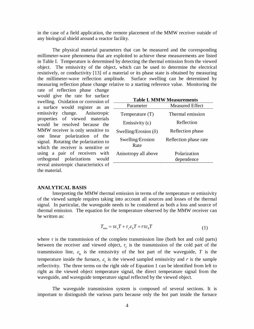
The physical material parameters that can be measured and the corresponding millimeter-wave phenomena that are exploited to achieve these measurements are listed in Table I. Temperature is determined by detecting the thermal emission from the viewed object. The emissivity of the object, which can be used to determine the electrical resistively, or conductivity [13] of a material or its phase state is obtained by measuring the millimeter-wave reflection amplitude. Surface swelling can be determined by measuring reflection phase change relative to a starting reference value. Monitoring the rate of reflection phase change would give the rate for surface swelling. Oxidation or corrosion of a surface would register as an emissivity change. Anisotropic properties of viewed materials would be resolved because the MMW receiver is only sensitive to one linear polarization of the signal. Rotating the polarization to which the receiver is sensitive or using a pair of receivers with orthogonal polarizations would reveal anisotropic characteristics of the material. ANALYTICAL BASIS

Interpreting the MMW thermal emission in terms of the temperature or emissivity of the viewed sample requires taking into account all sources and losses of the thermal signal. In particular, the waveguide needs to be considered as both a loss and source of thermal emission. The equation for the temperature observed by the MMW receiver can be written as:

(1)

where τ is the transmission of the complete transmission line (both hot and cold parts) between the receiver and viewed object, τc is the transmission of the cold part of the transmission line, εh is the emissivity of the hot part of the waveguide, T is the temperature inside the furnace, εs is the viewed sampled emissivity and r is the sample reflectivity. The three terms on the right side of Equation 1 can be identified from left to right as the viewed object temperature signal, the direct temperature signal from the waveguide, and waveguide temperature signal reflected by the viewed object.

The waveguide transmission system is composed of several sections. It is important to distinguish the various parts because only the hot part inside the furnace

Table I. MMW Measurements

Parameter Measured Effect

Temperature (T) Thermal emission

Emissivity (ε) Reflection

Swelling/Erosion (δ) Reflection phase

Swelling/Erosion Rate

Reflection phase rate

Anisotropy all above Polarization dependence

mm s c h hT T T r Tτε τ ε τε= + +

5

becomes a source of thermal emission. In addition, the hot part of the waveguide transmission will depend on the temperature. Consequently, the total transmission factor can be expressed as: (2) where the transmission factor is shown to be a function of temperature and τwd is the transmission through the window sealing the waveguide outside the furnace, τc is the transmission through the cold part of the waveguide, and τh(T) is the hot waveguide transmission inside the furnace which depends on temperature. The window and cold waveguide transmission are constant values at room temperature.

If the transmission line does not leak MMW radiation and the viewed sample is not transparent, then Kirchhoff’s law of thermal radiation relates the transmission line emissivity with its transmission and the viewed sample emissivity with its refection. These relations can be written as: (3) (4)

Since only the hot part of the transmission contributes to the temperature signal, it is only the emissivity of hot part of the transmission line that is of interest. Assuming that the fraction of the waveguide that is hot is given by a factor fh where the sum of the hot and cold factions is defined as equaling one (fh + fc = 1), then the hot transmission line emissivity can be derived from equations 2 and 3 as: (5)

Similarly the cold waveguide transmission can be derived from Equations 2 and 4 as: (6) where τo = τ(Troom) is the total transmission factor measured at room temperature. The MMW instrumentation setup can be characterized to obtain the values of all the parameters in Equation 1 not related to the viewed object. Using a thermocouple to obtain the furnace temperature, T, a measurement of the MMW temperature, Tmm, can then be used to obtain the viewed sample emissivity.

1s rε = −

1h hwd

f τετ

= −

( ) ( )wd c hT Tτ τ τ τ=

1ε τ= −

( )1 1c c o wdfτ τ τ= − −

6

Once the sample emissivity is known it can be related to the surface resistance and resistivity of the sample by the equations: (7) (8) where η = 377 Ω is the impedance of free space, Rs is the sample surface resistance, f is the MMW frequency, which is 137 GHz for the measurements here, µo is the permeability constant, and ρ is the sample resistivity.

Position Measurement Detecting the viewed object surface position displacement due to thermal expansion, swelling, or erosion is achieved by monitoring the reflected local oscillator (LO) signal emitted by the heterodyne receiver. The LO signal is a sine wave that on reflection from the viewed object will interfere with itself in the receiver mixer constructively or destructively depending on whether the refection is in phase or out of phase with the LO at the mixer. This in turn depends on the on the round trip path length between the receiver and viewed object. The signal will vary between a maximum and a minimum for every quarter wavelength change in distance to the viewed surface. The dependence on path length of this video signal is expressed by: (9) where Vo is the LO voltage generated in the mixer, Vr is the reflected LO signal from the viewed surface, and the phase shift of the reflected signal is given by: (10) where L is the path length to the viewed surface from the receiver and λ is the wavelength of the LO, which is 2.188 mm for the measurements here. It can be seen from these relations that a path length change of ¼ λ, 547 µm, would cause the reflected LO video signal to vary through a minimum-maximum-minimum range. Consequently, a sensitivity of about 50 µm (1/10 to a minimum to maximum change) to surface position would be possible. Higher frequency receivers would reduce this sensitivity to smaller displacements in proportion to operating frequency.

( )( )

2 2

2 2s s

s s

R Rr

R R

η

η

− +=

+ +

s oR fπ µ ρ=

4 coso rI V V δ∝

4 Lδ πλ

=

7

EXPERIMENTAL SETUP In the present work the generic MMW sensor configuration as shown in Figure 1

was implemented with two receivers to enable simultaneous orthogonal polarization observations for real time anisotropic material sensitivity. In addition, a beamsplitter was included in front of one of the receivers to provide an alternative approach for determining the viewed sample emissivity. In theory, it would be possible to determine the viewed object emissivity without the need for an independent thermocouple measurement of furnace temperature. The beamsplitter splits off a part of the thermal emission from the material being viewed to a side mirror which returns the emission to probe the sample. If the sample emissivity is less than one, then inserting the side mirror will increase the measured MMW receiver signal in proportion to the surface emissivity. This is referred to as the thermal return reflection method (TRR) [14]. The expression for the viewed surface refection in terms of the MMW signal measured with and without a return reflection is given by:

(11)

where κ is a parameter with a value between 0 and 1 introduced to take into account additional round trip transmission line losses that could be due to misalignment or geometrical surface figure imperfections of the viewed object, and rbs is the beamsplitter reflectivity. In studies of glass melts with a floating salt layer, κ was found to vary from 0.4 to 0.6 [15].

A schematic illustration of the laboratory implementation of the MMW thermal analysis hardware is shown in Figure 2 and Figure 3. The MMW wave receivers are heterodyne receivers that operate at a center frequency of 137 GHz (λ = 2.188 mm) with intermediate frequency (IF) amplifier bandwidth of 0.5-2.0 GHz making the effective frequency range 137 ±2 GHz. Receiver 2 is polarized perpendicular to Receiver 1. Receiver 1 views the electric field direction at the test specimen that is in the plane of Figure 2 and Receiver 2 views the electric field direction that is perpendicular to the plane of Figure 2.

Corrugated metallic waveguide (aluminum and brass) is used to propagate the MMW signals between the receivers and a miter mirror above the furnace where the waveguide material changes to smooth walled ceramic mullite (3Al2O3:2SiO2) that goes inside the electric furnace. The internal diameter of the waveguide increases from 20 mm (0.787”) at the receivers and chopper to 41 mm (1 5/8”) for the mullite waveguide going inside the furnace in the present experiments. Larger diameter helps reduce transmission line losses in the dielectric mullite waveguide. The length of the mullite waveguide was 53.3 cm (21”) of which 2/3 (fh = 0.667) was inside the furnace. A Teflon window is used to seal the waveguide section in the furnace as shown to allow a purge gas to be flowed through the waveguide into the furnace displace the air and prevent uncontrolled test specimen oxidation at high temperatures.

2 2 '

1 1 mm

bs mm

Trr Tκ τ

= −

8

The chopper with a flat reflective blade serves two functions. It allows both receivers to view the test specimen and also modulates the signals for synchronized detection with lock-in amplifiers. When the chopper blade is not in the waveguide, the

Figure 3. Photo of the MMW thermal analysis hardware setup at MIT. Major components are identified.

MMWReceiver

Waveguide

Mirror

TRR Mirror

Beamsplitter

WindowMMW

Receiver#2

#1

ChopperFurnace

purgegas

Test Specimen

View Dump

Figure 2. Schematic illustration of the MMW thermal analysis hardware setup.

9

furnace signals pass to and from Receiver 1. When the chopper blade moves inside the waveguide at an angle of 45º to the waveguide axis, it reflects the furnace signals to and from Receiver 2. Typically the chopping frequency is about 100 Hz. When the receivers are not viewing the furnace, the background laboratory temperature reference is viewed.

The other major hardware component in the setup is the beamsplitter in a four

port crossed waveguide block in front of Receiver 1. A fused quartz beamsplitter was polished to a thickness of 0.90 mm to be approximately 50% reflective at 137 GHz. Half the thermal emission from the test specimen is reflected to the side port and can be partially returned to the sample by a thermal return reflection (TRR) mirror. By repeatedly removing and replacing the TRR mirror on this port the thermal signal detected by Receiver 1 is modulated to a level that depends on the reflectivity of the test specimen, which in turn depends on the test specimen emissivity. The port opposite the TRR mirror is a signal dump port and not used. The viewing dump can be the laboratory by leaving this port open, as shown in the photo of Figure 3, or a MMW blackbody absorbing material. Data Acquisition Electronics

The data acquisition system, shown in Figure 4, uses a total of four lock-in amplifiers, two for each receiver referenced to the chopper frequency. One lock-in in each receiver is used to monitor the thermal signal, relative to room temperature, emitted by the hot specimen, and the other is used to monitor the reflected local oscillator video signal. The signal outputs of these lock-in amplifiers are connected to a National Instruments model USB-6215 analog to digital module for computer signal acquisition and processing using LabView software. A common ground plate through which all the signals are connected to the input of the A to D module was added, as shown in Figure 4, to solve a problem with an intermittent signal voltage offset that complicated the calibration.

L oc k-in A mplifiers

C ommon G round P late A to D Module

Figure 4. Data acquisition electronics for the dual 137 GHz MMW receiver system. A common ground plate solved a problem with an intermittent signal offset.

10

TEST SPECIMEN HOLDER An important accomplishment during the course of this work was finding a test

sample holding arrangement inside the mullite waveguide within the furnace that could prevent uncontrolled oxidation of the specimen at high temperatures without a permanent seal. This arrangement is detailed in Figure 5 and photos are shown in Figures 6 and 7. The test specimen inside the 41 mm diameter mullite waveguide rests on a 40 mm diameter, 6 mm (1/4”) thick alumina disk that is supported by a mullite tube segment with a 40 mm outside diameter and is 50 mm (2”) long. This stack of test specimen, alumina disk and mullite support tube is shown in Figure 6 with a 40 mm diameter,

20 mm thick graphite sample on top. The stack is inserted from the bottom of the mullite waveguide and held in place with a 3 mm (1/8”) alumina rod as shown in Figure 7. This arrangement allows easy insertion and removal of the test sample between high temperature furnace operations. It also holds the sample in alignment with the surface perpendicular to the waveguide axis for refection measurements.

A purge gas continually flows down the waveguide over the surface of the test specimen at a rate of 10 – 14 liters per minute (lpm) during high temperature furnace operation. Pure nitrogen was used

mullite waveguide

outer crucible

samplealumia

backing diskmullite tube

aluminasupport rod

Figure 5. Detail of test specimen support inside the furnace waveguide.

Figure 6. Photo of inner stack of graphite test specimen, alumina disk and mullite support tube. The test specimen is 40 mm in diameter and 20 mm thick

Figure 7. View of assembled test specimen inside furnace waveguide ready for a high temperature test.

11

as the purge gas in these experiments. After the first test with a graphite sample heated to 1300 ºC it was found that the sample surface was slightly discolored on one side. This was an indication that the purge gas flow was not uniform around the circumference of the sample as the gas flow exited the waveguide, allowing some backward diffusion of air on one side. To compensate for this effect an outer containment of the purge gas flow was implemented by inserting the end of the waveguide with the sample into a 73 mm (2 7/8”) diameter, 150 mm (6”) tall cylindrical Coors mullite crucible. In subsequent high temperature tests this appeared to solve the problem with backward air diffusion. WAVEGUIDE THERMAL EXPANSION

The part of the waveguide that is inside the furnace is heated to high temperatures along with the test specimen. Consequently the waveguide will expand, changing the path length of the signals between the receivers and test specimen. This causes a significant change in the video signal, which depends on the phase of the reflected signal as previously described. The signal will cycle through minimum-maximum for every 547 µm change in path length.

Figure 8 shows the detected coherent reflection, labeled Video 1, as recorded by Receiver 1 when a graphite test specimen was heated to 1300 °C. The furnace temperature is shown by the upper blue plot as obtained by a Type S thermocouple. The video signal consists of a number of fringes as the heated waveguide expands and then contracts as it is cooled down. The contribution of the expansion of the test specimen is not considered to be significant since it is thin in comparison to the length of waveguide

0

500

1000

1500

0 0.2x105 0.4x105 0.6x105 0.8x1050

0.5

1.0

1.5

1233

21

Video 1Signal

FurnaceTemperature

Time (s)

Tem

pera

ture

(o C)

Cohe

rent

Ref

lect

ion

(rela

tive)

Fugure 8. Expansion of the mullite waveguide inside the furnace shown by interference fringes recorded in the lower plot due to reflection of the 137 GHz local oscillator signal from the a graphite test specimen.

12

that is exposed to high temperature. The fringes are labeled 1 through 3 on the plot. A fourth fringe not completely formed at the maximum temperature is not labeled. Notice that when the temperature of the furnace is held constant at 520 and 1300 °C, the video signal also does not change confirming that this fringe pattern is due to thermal expansion.

The observed total fringe count of slightly over 3.5 on heat up to 1300 °C corresponds to a waveguide expansion of approximately 2 mm. This is consistent with a thermal expansion coefficient of 5.4 × 10-6 /°C for mullite [16] and a 30 cm length of waveguide exposed to high temperature as in the present setup. An important capability of MMW monitoring is demonstrated here to be able to observe surface swelling or erosion with sensitivity of the order of 50 µm at constant temperature. In a reactor operating at constant temperature, the observation of fringe shifts such as these would indicate material swelling creep or possible erosion if the surface is in a corrosive environment. Even with changing temperature, having the calibration curve for the waveguide expansion, it should be possible to determine the contribution of the viewed material dimension change on the fringe pattern if it is a significant fraction of one fringe. EXPERIMENTS

Initial Graphite and Silicon Carbide Measurements

A number of experimental campaigns with isotropic graphite and silicon carbide

test specimens were carried out in the first year. Primarily, these tests were to shake down and gain experience the MMW instrumentation system. Much was learned about the performance of the MMW instrumentation and an interesting discovery was made that not all graphite is alike in the MMW spectrum.

Figure 9 shows the temperature measurement record for heating a high strength, wear resistant graphite test specimen of grade GR001CC manufactured by Graptek LLC with dimensions as shown in Figure 5. The heating cycle is the same one as in Figure 8 to 1300 °C lasting about 23 hours with a 36 minute pause at 520 ºC during warm up and then a one hour hold at 1300 ºC after which the furnace was turned off and allowed to cool overnight. The upper plot (blue) is half the furnace temperature as measured by a thermocouple located beside the mullite waveguide inside the furnace and the lower overlapping plots (red and black) are the millimeter-wave receiver temperatures as calibrated at the Teflon window.

The MMW temperatures are much lower than the furnace temperature (MMW at 544 ºC for the furnace at 1300 ºC) because the MMW thermal signals are a product of emissivity and temperature (εT). Graphite has a very low emissivity (ε<<1) making the observed MMW temperature much lower than the furnace temperature. Actually the graphite MMW signal is even lower that plotted because a large part of the thermal signal in this case is due to hot mullite waveguide emission as shown by Equation 1. From waveguide transmission measurements (~0.86) made before the furnace warm-up and the

13

length of hot waveguide inside the furnace over half the MMW signal temperature can be attributed to waveguide emission.

Another indication of the low emissivity of graphite is the increase in the MMW temperatures when the TRR mirror is inserted for the Receiver 1 view. This was done during the temperature flat tops as shown in Figure 9. It is the ability to observe the emissivity of the test specimens that makes this instrumentation uniquely capable for high temperature materials degradation studies.

The long downward spikes on these MMW temperature plots occurred when both receiver views were blocked at the Teflon window by a known black body temperature to calibrate the receiver response. With the calibration, both receivers pretty much see the same MMW temperature, which would be expected for an isotropic material. In some of the tests the receiver signals were offset at different temperatures when viewing isotropic test specimens’, which was caused by a slight misalignment of one receiver view into the waveguide relative to the other, making the waveguide transmission losses different for the two receivers. Silicon carbide samples were obtained from Ortech, Inc., which were molded into 40 mm diameter disks, 10 mm thick to fit inside the mullite waveguide. A typical graphite sample is shown with one of the silicon carbide samples in Figure 10. Except for the less thick size of the silicon carbide, the outward dark gray visible appearance of both materials is similar. However, in the MMW range of the electromagnetic spectrum

0

250

500

750

0 0.2x105 0.4x105 0.6x105 0.8x105

Half Furn. Temp.Rec1 Temp.Rec2 Temp.TRR

Calibrations

Time (s)

Tem

pera

ture

(o C)

Figure 9. Temperature signals for heating grade GR001CC Graptek, LLC graphite sample to a maximum furnace temperature of 1300 ºC.

14

the appearance of the two materials is markedly different, as shown in Figure 11. Here we compare the MMW temperatures observed by Receiver 1 orginally shown in Figure 9 for a graphite sample with another plot obtained for a silicon carbide sample heated to the same maximum furnace temperature flat top of 1300 ºC. The silicon carbide maximum MMW temperature is about 1200 ºC, almost the furnace temperature while the graphite MMW temperature is less than half. Analysis shows that the 137 GHz emissivity of graphite is less than 0.1 while the emissivity of the Ortech silicon carbide is over 0.9.

0

400

800

1200

0 2 4 6 8 10 12calibrations

TRR

TRR

Graphite

SiC

Time (hr)

Milli

met

er-W

ave

Emiss

ion

(o C)

0

400

800

1200

0 2 4 6 8 10 12calibrations

TRR

TRR

Graphite

SiC

Time (hr)

Milli

met

er-W

ave

Emiss

ion

(o C)

Figure 11. Comparing silicon carbide with graphite, Ortech, Inc silicon carbide and GR001CC Graphtek graphite up to a maximum furnace temperature of 1300 ºC.

Figure 10. Photos of (a) graphite, 40 mm diameter by 20 mm thick and (b) silicon carbide, 40 mm diameter by 10 mm thick that were used in tests with the MMW instrumentation.

15

Further confirmation of the MMW difference between graphite and silicon carbide is given by the TRR measurement shown in Figure 12. Here the TRR portions of the plots shown in Figure 11 are blown up to show the detail of the temperature change. When the TRR mirror is inserted three times the increase in observed MMW temperature is much higher for graphite, indicating that the reflectivity of graphite at 137 GHz is also much higher and through Equation 4 indicates that the emissivity of graphite is lower. If the parameter κ can be determined, then the ratio of the ratio of the low to high TRR temperature can be used in Equation 11 with Equation 4 to obtain emissivity.

Comparison of Different Graphite Grades Graphtek, UCAR, & B-Reactor Graphites

Measurements were taken on a number of similar isostatically molded graphite specimens: Graphtek GR001CC, UCAR PGX, and Pacific Northwest Laboratory (PNNL) B-reactor graphite, which is a treated version of UCAR PGX. According to the manufactures data, the room temperature resistivity of the Graptek sample was slightly higher than that for the UCAR PGX grade at 13.9 µΩm versus 10.1 µΩm, respectively. These samples where heated to a temperature of 1300 ºC, allowed to cool down overnight, and then reheated to 520 ºC the next day. The MMW thermal emissions at 520ºC before and after high temperature exposure were compared. In general, all the grades had low MMW emission temperatures because of low graphite emissivity at MMW frequencies as previously noted. There were only slight, but notable variations among the various grades.

The MMW emission for the GR001CC sample along with the furnace

temperature is shown in Figure 13 for two furnace warm ups taken one day apart. Only the Receiver 1 signal and furnace temperatures for the flat top data at 520 ºC are plotted here. The first day warm up is plotted as dashed curves that continue on to a maximum of 1300 ºC, not shown off the left of the graph. The second day’s warm up are solid lines

525

550

575

600

7.4 7.5 7.6

Time (hr)

MM

W E

mis

sion

(o C)

525

550

575

600

7.4 7.5 7.6

Time (hr)

MM

W E

mis

sion

(o C)

GraphiteTRR = 584 oC

543 oC

1190

1195

1200

1205

6.85 6.95

Time (hr)

MM

W E

mis

sion

(o C)

1190

1195

1200

1205

6.85 6.95

Time (hr)

MM

W E

mis

sion

(o C)

Silicon CarbideTRR = 1200 oC

1197 oC

Figure 12. Comparison of the TRR signal for graphite and silicon carbide at a furnace temperature of 1300 ºC showing that the MMW emissivity of graphite is much lower than that for silicon carbide.

16

that decrease after the flat top temperature. It is readily evident that the MMW emissivity of the Graphtek graphite increased after the first test. The increased in MMW temperature was 15 ºC from 162 to 177 ºC at a furnace temperature of 520 ºC. This would correspond to a much larger change in the graphite conductivity that indicates heat induced surface changes. Visible inspection of the sample after these tests did not reveal a significant change in the visible surface, only a slight difference in the macroscopic non uniformity of the surface darkness.

Examination of the test specimens before and after the experiments did not reveal any

significant visible changes, but the MMW emission shows a noticeable change in dielectric behavior of the GR001CC sample. This is somewhat contrary to expectations since according to the manufacturer parameters in Table I the GR001CC is denser, purer graphite. However, this observation supports the argument that properties alone do not determine the suitability of a particular grade of graphite for an extreme environment, but other factors such as the details of the manufacturing process will also influence performance [2].

The two other samples of UCAR PGX graphite with one produced for the PNNL B-Graphite reactor were tested in the same way to 1300 ºC as the Graphtek sample. These samples were provided as 2 mm thick, 95 x 19 mm rectangles, and were cut to fit inside the 41 mm diameter mullite waveguide. The thickness of a graphite test sample does not matter in these measurements since it is opaque at MMW frequencies. The resulting data is shown in Figures 15 and 16. The MMW temperature of these graphite samples were lower and did not change after the samples were cycled to 1300 ºC. The temperature of

0

100

200

300

400

0 3000 6000 9000 12000

EmissivityIncrease

MMW Temperature

1/2 Furnace Temperature

Time (s)

Tem

pera

ture

(o C)

Figure 13. Reheat of Graphtek GR001CC graphite (solid curves) compared to before 1300 ºC exposure (dashed curves).

17

the PNNL sample was 152 ºC for a furnace temperature of 520 ºC. The lower emissivity of this graphite grade is consistent with it having a lower resistivity. The MMW measurement confirms that the B-Graphite reactor material is of higher quality and does not degrade with thermal cycling.

0

100

200

300

400

0 4000 8000 12000 16000

Emissivityminor change

MMW Temperature

1/2 FurnaceTemperature

Time (s)

Tem

pera

ture

(o C)

Figure 16. Reheat of PNNL B-reactor graphite (solid) compared to before 1300 ºC exposure (dashed).

0

100

200

300

400

0 5000 10000 15000

Emissivityminor change

MMW Temperature

1/2 FurnaceTemperature

Time (s)

Tem

pera

ture

(o C)

Figure 14. Reheat of UCAR PGX graphite (solid curves) compared to before 1300 ºC exposure (dashed curves).

18

SGL NBG17 & R7340 Graphite Other graphite materials were acquired from the SGL Group for more extensive

studies. There were two grades studied: a nuclear reactor grade NBG17 and fine grade R7430 graphite that is used in the glass molding industry. These materials arrived in 12 inch (305 mm) long 1.57 inch (40mm) diameter rods that were sliced into 0.787 inch (20 mm) thick pucks for insertion into the mullite waveguide inside the furnace. The measurements were carried out are summarized in Tables II and III.

Table II. NBG17 Graphite Measurements Sample-Test Furnace Rec. #1 Fraction Rec. #2 Fraction Rec1/Rec2 (deg C) (deg C) (deg C )

1-1 523.7 123.6 0.295 164.4* 0.365* 1-2 529.9 122.4 0.289 158.5* 0.348*

1248.7 379.7 0.380 477.3* 0.444* 1-3 520.7 112.7 0.271 121.1 0.271 1.000

2-1 507.5 112.0 0.276 117.4 0.269 1.025 2-2 1239.8 334.4 0.337 368.8 0.346 0.975 2-3 508.0 104.1 0.256 108.4 0.248 1.032

3-1 513.1 117.2 0.285 114.1 0.258 1.104

1284.5 352.0 0.343 362.1 0.328 1.045 3-2 504.4 104.8 0.260 106.4 0.245 1.059 3-3 508.2 106.1 0.261 108.1 0.247 1.055

1286.0 359.0 0.349 367.8 0.333 1.049 *Data suspect, taken before grounding plate used to eliminate signal offset.

The Table II lists data gathered on three NBG17 samples thermally cycled up to

three times each and Table III lists data on two R7340 samples thermally cycled up to 4 times each. Each thermal cycle corresponds to heating over one day and cooling over night. The samples were continually flushed with dry nitrogen to prevent oxidation. The second column in the tables lists the furnace thermocouple reading when the furnace temperature was held constant (0.5 – 1.5 hours) for temperature readings by MMW Receiver #1 and #2 given in columns 3 and 5. The MMW temperatures are lower because, as stated above, the thermal emission is a product of emissivity and temperature (εT) with graphite emissivity much less than 1. The actual thermal emission from the graphite sample is lower than the receiver measurement because the hot part of the waveguide also contributes emission to the measurement as described in Equation 1. The Fraction columns to the left of the receiver temperatures give the fraction of the furnace temperature that each receiver registers. They should be the same for the two receivers for these samples which do not have anisotropy, and generally are within a few per cent.

Two constant temperature levels were examined at nominal furnace controller

settings of 525 and 1250 °C. The listed temperatures in the first column are from a

19

second thermocouple located adjacent to the outside of the waveguide in the furnace and differ slightly from the furnace control setting. The higher temperature readings are highlighted in bold. The results are generally reproducible to repeated thermal cycling and from sample to sample. There was no thermal cycling degradation for either of these graphite grades as was seen in the Graphtek sample above. The absolute temperature fraction was about the same for both grades, within about a few per cent of experimental error. The observation that the faction of the furnace temperature that is registered by the receivers increases for the higher temperature suggests that the mullite waveguide losses are increasing with temperature since the emissivity of graphite would not change this much with temperature. This is the subject of additional investigation in the next section. Table III. R7430 Graphite Measurements Sample-Test Furnace Rec. #1 Fraction Rec. #2 Fraction Rec1/Rec2

(deg C) (deg C) (deg C ) 1-1 507.8 124.3 0.295 123.3 0.282 1.044 1-2 509.1 124.3 0.289 122.6 0.280 1.031

1286.9 425.9 0.414 449.6 0.406 1.019 1-3 507.8 121.6 0.299 116.5 0.267 1.122

1285.4 419.2 0.408 431.5 0.390 1.045 1-4 505.1 122.8 0.304 120.9 0.278 1.091

2-1 515.0 110.1 0.267 111.9 0.253 1.058

1284.9 412.6 0.401 406.8 0.368 1.090 2-2 505.1 112.9 0.279 118.5 0.273 1.024

1285.0 409.8 0.399 410.0 0.371 1.074 2-3 507.4 116.4 0.287 119.2 0.273 1.050

Mullite Waveguide Degradation with Temperature The mullite waveguide degradation of MMW transmission with temperature was quantified by using the known temperature behavior of the resistivity of NBG-17 graphite provided by the manufacture, shown in Figure 17, and making the assumption that the change in mullite transmission is linear with temperature. The linear equation for the mullite waveguide transmission as a function of temperature was thus obtained by determining the slope from the high temperature measurements and the y-intercept from a waveguide transmission measurement made at room temperature. No assumption was necessary on the actual value of the graphite surface resistance at 137 GHz and in fact this parameter was determined once the mullite waveguide was characterized for high temperature MMW transmission. The relationship between DC resistivity and high frequency surface resistance is given by Equation 8. The two flat top temperatures at 525 and 1250 °C were used for the determination of the hot waveguide degradation slope when the furnace was held constant for up to an

20

hour and the observed graphite sample could be assumed to be in equilibrium with the thermocouple temperature. Equations 1 - 6 where solved for transmission, τ, using the measured MMW temperatures and the increase in the graphite resistivity between the two temperatures of 6.5 % taken from the plot in Figure 17. The difference in τ is obtained without direct knowledge the actual resistivity. The actual transmission at high temperature was then determined by extrapolating back to the room temperature waveguide transmission measurement.

The resulting plot for the Receiver 1 waveguide is shown in Figure 18. The error bars at 525 and 1250 °C are the standard deviation of the MMW temperature measurements taken on four different days. Four separate transmission measurements at room temperature waveguide were also taken, but the error bar at 20 °C is too small to resolve on the scale of Figure 18. The total hot and cold waveguide and window transmission at 137 GHz deceases from 0.845 ± 0.001 to 0.791 ± 0.01 over the temperature range of 20 to 1250 °C. The degradation slope of only the hot part of mullite waveguide was determined through Equations 2 and 5 to be -4.4 x 10-5 /m/°C using the hot waveguide fraction fh = 0.667. This slope can be scaled to other frequencies and waveguide diameters by the known scaling of dielectric waveguide attenuation that is proportional to the square of frequency and the inversely proportional to the third power of waveguide diameter τ∝ F2/D3 [17].

Figure 17. The DC resistivity of SGL NBG-17 graphite as a function of temperature.

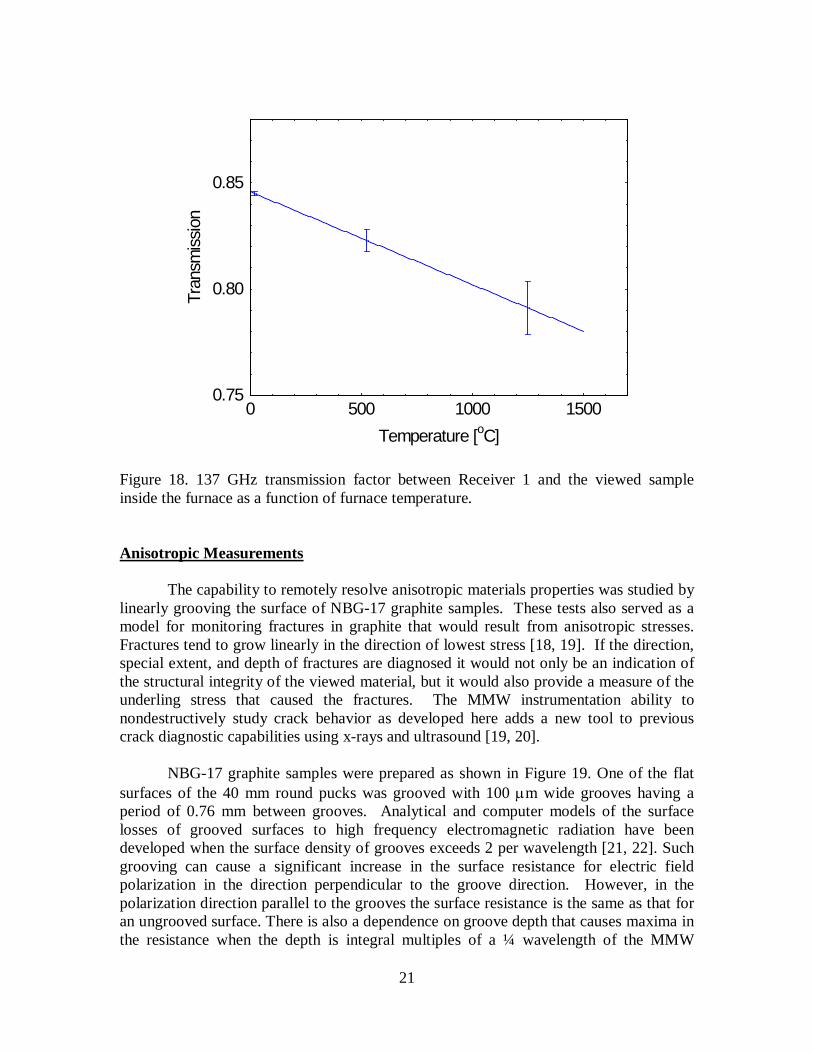
21

0.75

0.80

0.85

0 500 1000 1500Temperature [oC]

Tran

smiss

ion

Figure 18. 137 GHz transmission factor between Receiver 1 and the viewed sample inside the furnace as a function of furnace temperature. Anisotropic Measurements The capability to remotely resolve anisotropic materials properties was studied by linearly grooving the surface of NBG-17 graphite samples. These tests also served as a model for monitoring fractures in graphite that would result from anisotropic stresses. Fractures tend to grow linearly in the direction of lowest stress [18, 19]. If the direction, special extent, and depth of fractures are diagnosed it would not only be an indication of the structural integrity of the viewed material, but it would also provide a measure of the underling stress that caused the fractures. The MMW instrumentation ability to nondestructively study crack behavior as developed here adds a new tool to previous crack diagnostic capabilities using x-rays and ultrasound [19, 20]. NBG-17 graphite samples were prepared as shown in Figure 19. One of the flat surfaces of the 40 mm round pucks was grooved with 100 µm wide grooves having a period of 0.76 mm between grooves. Analytical and computer models of the surface losses of grooved surfaces to high frequency electromagnetic radiation have been developed when the surface density of grooves exceeds 2 per wavelength [21, 22]. Such grooving can cause a significant increase in the surface resistance for electric field polarization in the direction perpendicular to the groove direction. However, in the polarization direction parallel to the grooves the surface resistance is the same as that for an ungrooved surface. There is also a dependence on groove depth that causes maxima in the resistance when the depth is integral multiples of a ¼ wavelength of the MMW

22

frequency when looking straight down on the sample surface (normal incidence) [22]. The groove depth chosen for the first sample is shown in Figure 19. It had groove depth of 1.65 mm near a perpendicular polarization maximum for surface resistance at ¾ wavelength depth.

Heating this sample showed a significant difference, as expected, in the MMW temperature between the two polarizations monitored by Receivers 1 and 2. Figure 20 shows the results when the sample was heated to 525 °C. The sample was first heated with the grooves oriented parallel to the electric field polarization of Receiver 1 as shown by the graph on the left. The observed Receiver 1 temperature of 129 °C was similar to the ungrooved samples while Receiver 2 registered a higher temperature. After cool down the sample was rotated 90° and reheated to the same furnace temperature. This time the Receiver 1 temperature increased to 170 °C while Receiver 2 decreased to the lower temperature as shown on the right. The 30% increase in the surface temperature for polarization perpendicular to the grooving over a smooth surface actually corresponds to a much higher change in surface resistivity once the contribution from the waveguide emission is in taken into account. This is analyzed below. Two more grooved samples of NBG-17 graphite were prepared with different groove depths of 1 and 2 mm to investigate the MMW temperature anisotropy as a function of depth. These measurements are shown in Figure 21 for the three groove depths of 1, 1.65, and 2 mm going from the bottom graph to the top. The furnace temperature was taken up to a maximum of 1250 °C for this study. It is evident that the temperature anisotropy increases and then decreases as the groove depth is increased through the ¾ wavelength depth near 1.65 mm. The emissivities can be quantified by solving the Equation 1 – 6 for emissivity and plugging in the experimental values to take into account the waveguide contributions to the thermal signal:

40 mm 0.1 mm

1.65

0.76a) b)

Figure 19. Details of the grooving in the graphite samples used for anisotropic studies; a) top view of the surface groove distribution cut into a graphite puck like the one shown in Figure 10a, b) groove dimensions of the first sample tested.

23

(12)

Tables VI and V list the constant and temperature dependent (at 525 °C) transmission line parameters that were defined in Equations 1 – 6 and that are needed for solving Equation 12. Table VI lists the MMW temperatures from Figure 21 at the 525 °C flat top and the resulting emissivities and surface resistances that were calculated from the measurements. The emissivities and surface resistances at 1250 °C are by definition, from the waveguide calibration using the plot in Figure 17, 6.5 % higher.

The Receiver 1 measurements with the electric field polarization parallel to the

grooves are all similar and correspond to a smooth ungrooved surface, which was confirmed by turning over the graphite puck with 2 mm grooves and observing its smooth side as listed below the 2 mm entry in Table VI. The average of all these values gives an emissivity of 5.1 ±0.5%, which can be converted into a surface resistance of 5.3 Ohms through the use of Equation 7. This surface resistance is higher by a factor of about 2.5 than what would be calculated by Equation 8 and the dc measured resistivity from Figure 17 of about 7.5 x 10-6 Ohm-m at 525 °C. This result is not too different for a measurement made by Kasparek etal [23] at 140 GHz of a graphite grade used in thermonuclear fusion energy experiments in Germany. The difference from the DC value is attributed to microscopic surface roughness that causes the high frequency skin depth to differ from the ideal behavior represented by Equation 8 and is commonly observed with other conductors at millimeter-wavelengths [24].

Figure 20. MMW receiver temperatures observed at a furnace temperature of 525 °C with a sample of NBG-17 graphite linearly groove structure on viewed surface as shown in Figure 19. The graph on the right shows the case for Receiver 1 E-field direction parallel to the grooves and the graph on the left shows the case for the E-field of Receiver 1 perpendicular to the grooves as illustrated by the inserts

( )( )1

mm c hs

h

T TTτ τ ε

ετ ε− +

=−

24

0

200

400

600

0 5 10 15

Rec. 1

Rec. 2

1/2 Furn. Temp.1.65 mm

Tem

pera

ture

[o C]

0

200

400

600

0 5 10 15

2 mm grooves

0

200

400

600

0 5 10 15

1 mm

Time [hr]

Figure 21. MMW receiver temperature anisotropy shown for three different groove depths of 1, 1.65, and 2 mm from bottom to top. The grooves were oriented parallel to the electric field view of Receiver 1 and perpendicular to Receiver 2.

25

Table IV. Constant Instrumentation Parameters Parameter Value

Receiver 1

Receiver 2

τo 0.845 ± 0.001 0.869 ± 0.005 τwd 0.98

0.98

fh 0.667

0.667 τc 0.899

0.916

Table V. Temperature Dependent Parameters at 525 °C Parameter Value

Receiver 1

Receiver 2

τ 0.823 ± 0.005 0.846 ± 0.01 εh 0.107

0.912

Table VI. NBG-17 Grooved Graphite Anisotropic Emissivity and Surface Resistance Resolved at 137 GHz and 525 °C

Receiver 1 Receiver 2

Groove Depth

MMW Temperature Emissivity

Surface Resistance

MMW Temperature Emissivity

Surface Resistance

[mm] [ °C]

[Ohms] [ °C]

[Ohms] 1 121 0.049 4.7 134 0.112 11.2

1.65 120 0.046 4.5 168 0.195 20.5 2 123 0.054 5.3 139 0.123 12.4

smooth 125 0.058 5.6 average

0.051 5.3

error bar

± 0.005 ± 0.05

± 0.005 ± 0.05

Receiver 2 measurements with the electric field perpendicular to the grooves show a MMW temperature that is hotter, corresponding to surface emissivity and resistance 2 to 4 times higher after waveguide contributions are taken into account. The observed normalized increase in surface resistance relative to the parallel groove direction is plotted as circle points in Figure 22 as a function of depth normalized to the MMW wavelength. For good conductors, surface resistance is linearly proportional to emissivity, which in turn is equivalent to absorption loss for an opaque material. The error bars in this plot result from those in the bottom row of Table VI. The dashed curve

26

is a theoretical calculation for an aluminum grooved surface at 158 GHz taken from Plaum etal [22]. The cycling of the normalized loss through maxima at ¼ wavelength multiples of the depth is clearly seen in the experimental and theoretical data. The lower relative loss peak for graphite is likely due to its much lower conductivity, which would decrease a resonance dependent effect. The peaking however is well above the signal to noise ratio of the measurement as is also evident in Figure 21. This could be exploited in a by a real time monitoring diagnostic to provide depth growth information on developing fractures without an absolute calibration of the instrumentation.

Silicon Carbide Coated The SGL Group provided several wafers of NBG-17 graphite coated with a thin silicon carbide layer, a composite material that is being developed for a high temperature reactor environment. Three different surface coating processes were used that resulted in surfaces that were called amorphous, good crystals, and powdered. These samples were heated to 1250 °C and analyzed for emissivity as previously described. The results are listed in Table VII along with the measurement for uncoated NBG-17 graphite at 1250 °C. The observed emissivities are much closer to what would be expected for graphite than for bulk silicon carbide. Recall that measurements comparing the emissivity of silicon carbide and graphite in Figure 11 indicated that the silicon carbide emissivity is on the order of 0.9. The thin silicon carbide coating on these wafers is largely transparent at 137 GHz. Of the several coatings, the powdered one has the lowest emissivity suggesting that is more transparent or thinner. These MMW measurements

0

2

4

6

8

0 0.2 0.4 0.6 0.8 1.0Normalized Depth

Norm

alize

d Lo

ss

Figure 22. Normalized losses as a function of groove depth normalized to wavelength. Points are for experimental data for NBG-17 graphite and dashed plot for grooved aluminum surface from Plaum etal [22]

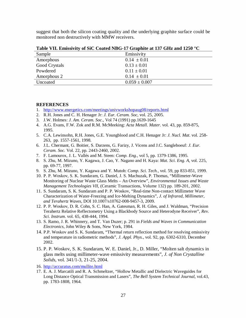
27

suggest that both the silicon coating quality and the underlying graphite surface could be monitored non destructively with MMW receivers. Table VII. Emissivity of SiC Coated NBG-17 Graphite at 137 GHz and 1250 °C Sample Emissivity Amorphous 0.14 ± 0.01 Good Crystals 0.13 ± 0.01 Powdered 0.11 ± 0.01 Amorphous 2 0.14 ± 0.01 Uncoated 0.059 ± 0.007 REFERENCES 1. http://www.energetics.com/meetings/univworkshopaug08/reports.html 2. R.H. Jones and C. H. Henager Jr: J. Eur. Ceram. Soc, vol. 25, 2005. 3. J.W. Holmes: J. Am. Ceram. Soc., Vol 74 (1991) pp.1639-1645 4. A.G. Evans, F.W. Zok and R.M. McMeeking: Acta Metall. Mater. vol. 43, pp. 859-875,

1995. 5. C.A. Lewinsohn, R.H. Jones, G.E. Youngblood and C.H. Henager Jr: J. Nucl. Mat. vol. 258-

263, pp. 1557-1561, 1998. 6. J.L. Chermant, G. Boitier, S. Darzens, G. Farizy, J. Vicens and J.C. Sangleboeuf: J. Eur.

Ceram. Soc. Vol. 22, pp. 2443-2460, 2002. 7. F. Lamourox, J. L. Vallés and M. Steen: Comp. Eng., vol 5, pp. 1379-1386, 1995. 8. S. Zhu, M. Mizuno, Y. Kagawa, J. Cao, Y. Nagano and H. Kaya: Mat. Sci. Eng. A, vol. 225,

pp. 69-77, 1997. 9. S. Zhu, M. Mizuno, Y. Kagawa and Y. Mutoh: Comp. Sci. Tech., vol. 59, pp 833-851, 1999. 10. P. P. Woskov, S. K. Sundaram, G. Daniel, J. S. Machuzak, P. Thomas, “Millimeter-Wave

Monitoring of Nuclear Waste Glass Melts – An Overview”, Environmental Issues and Waste Management Technologies VII, (Ceramic Transactions, Volume 132) pp. 189-201, 2002.

11. S. Sundaram, S. K. Sundaram and P. P. Woskov, “Real-time Non-contact Millimeter Wave Characterization of Water-Freezing and Ice-Melting Dynamics”, J. of Infrared, Millimeter, and Terahertz Waves, DOI 10.1007/s10762-008-9457-3, 2009.

12. P. P. Woskov, D. R. Cohn, S. C. Han, A. Gatesman, R. H. Giles, and J. Waldman, “Precision Terahertz Relative Reflectometry Using a Blackbody Source and Heterodyne Receiver”, Rev. Sci. Instrum. vol. 65, 438-444, 1994.

13. S. Ramo, J. R. Whinnery, and T. Van Duzer; p. 291 in Fields and Waves in Communication Electronics, John Wiley & Sons, New York, 1984.

14. P.P. Woskov and S. K. Sundaram, “Thermal return reflection method for resolving emissivity and temperature in radiometric methods”, J. Appl. Phys., vol. 92, pp. 6302-6310, December 2002.

15. P. P. Woskov, S. K. Sundaram, W. E. Daniel, Jr., D. Miller, “Molten salt dynamics in glass melts using millimeter-wave emissivity measurements”, J. of Non Crystalline Solids, vol. 341/1-3, 21-25, 2004.

16. http://accuratus.com/mullite.html 17. E. A. J. Marcatili and R. A. Schmeltzer, “Hollow Metallic and Dielectric Waveguides for

Long Distance Optical Transmission and Lasers”, The Bell System Technical Journal, vol.43, pp. 1783-1808, 1964.

28

18. A. Hodgkins, T. J. Marrow, P. Mummery, B. Marsden and A. Fok, “X-ray tomography observation of crack propagation in nuclear graphite”, Materials Science and Technology, vol. 22, pp. 1045-1051, 2006.

19. H. Kakui and T. Oku, “Crack Growth Properties of Nuclear Graphite Under Cyclic Loading Conditions”, Journal of Nuclear Materials, vol. 137, pp. 124-129, 1986.

20. A.S. Erikssona, J. Mattsson, A.J. Niklasson, “Modelling of ultrasonic crack detection in anisotropic materials”, NDT&E International, vol. 33, pp. 441-451, 2000.

21. E. A. Nanni, S. K. Jawla, M. A. Shapiro, P. P. Woskov, R. J. Temkin, “Low-loss Transmission Lines for High-power Terahertz Radiation”, J Infrared Milli Terahz Waves, vol. 33, pp. 695-714, 2012.

22. B. Plaum, E. Holzhauer, C. Lechte, “Numerical Calculation of Reflection Characteristics of Grooved Surfaces with a 2D FDTD Algorithm”, J Infrared Milli Terahz Waves, vol 32, pp. 482-495, 2011.

23. W. Kasparek, A. Fernandez, F. Hollmann, and R. Wacker, Measurements of Ohmic Losses of Metallic Reflectors at 140 GHz Using a 3-Mirror Resonator Technique, Int. J. of Infrared and Millimeter Waves, vol. 22, 1695-1707, 2001.

24. P.B. Bharitia and I. J. Bahl, Millimeter-Wave Engineering and Applications, p. 202, John Wiley & Sons, New York, 1984.

29

APPENDIX

Millimeter-Wave Receiver Construction Details and Parts List Receiver Wiring

The wiring of one of the Millimeter-Wave receivers is detailed here. The millimeter-wave receiver is heterodyne receiver for both detecting thermal radiation and a coherent reflected leaked local oscillator signal. Its center frequency of operation is 137 GHz with sidebands at 135.0 – 136.5 GHz and 137.5 – 139.0 GHz. There are two outputs: the Intermediated Frequency (IF) output containing the thermal signal in the two sidebands and the Video output with the coherent reflected signal. Both these outputs were modulated on and off by the internal chopper in an original configuration as shown in Figures A1 and A2, but when used with two receivers the chopper was moved to the input of the 4-wave block as shown in Figure 2 of the main text. Lock-in amplifier detection, referenced to the chopper frequency, is used to monitor these two signals. The IF signal is related to the temperature and emissivity of the viewed surface and the Video signal is related to surface position and movement.

The receiver electronic circuit is illustrated in Figure A1. The heart of the circuit

is a MilliTech mixer and local oscillator (LO) at a frequency of 137 GHz. The LO is powered by 15 V DC. A bias tee connected to the IF output of the mixer divides the heterodyne downshifted signal into a DC and an RF/IF part. The DC signal goes to the Video output connector. The IF signal goes into a pair of low noise amplifiers with a bandwidth of 0.5 – 2.0 GHz. These amplifiers are powered by 15 and 12 V DC. After amplification the IF signal is rectified by a microwave diode detector and connected to the IF output connector.

On the millimeter-wave input side of the mixer, a WR-6 rectangular waveguide connects the mixer to a horn, which is inserted into an aluminum corrugated waveguide transition to the chopper assembly in dielectric G-10 waveguide. The chopper periodically blocks the mixer view to modulate the IF and Video signals for lock-in detection. When the metallic chopper blade blocks the waveguide, the mixer view is reflected to the side to view a millimeter-wave blackbody (eccosorb). This blackbody acts as the reference temperature for the IF thermal measurements. A type k thermocouple is located nearby so this temperature can be recorded.

30

Figure A1. The wiring circuit for one of the two heterodyne receivers used in this work.

Figure A2. Receiver circuit component layout. Four-port waveguide block not shown off to right. Connection to Measurement System

Connection of the Millimeter-Wave receiver to other instrumentation for thermal and reflection measurements is shown in Fig. A3. The chopper controller is connected to the chopper connector and the reference output from this controller is connected to the reference input of the two lock-in amplifiers. The chopper is nominally set at 100 Hz chopping frequency.

31

The TC output is connected to a readout unit for type k thermocouples with an analog signal output proportional to temperature. This analog signal is an input to one of the channels of the Analog to Digital (A to D) data acquisition system.

The IF signal is input to one of the lock-in amplifiers. This signal is also input, in parallel by a BNC tee, to a digital voltmeter (DVM). The time constant on the lock-in should be set to 100 or 300 milliseconds. The sensitivity scale should be set to about 2 mV. The analog output from the lock-in is input to another channel of the A to D data acquisition system.

The Video signal is input to a second lock-in amplifier. The time constant should be set to 30 or 100 milliseconds. The sensitivity is set to about 1 mV. The analog output of this lock-in is input to another A to D channel of the acquisition system.

Figure A3.Millimeter-wave receiver connection diagram for thermal and reflection measurements from one receiver. These signal acquisition electronics are photographed in Figure 4 for two receivers.

32

Table A1. Millimeter-Wave Receiver Parts Component Vendor 137 GHz Millimeter-Wave Receiver Front End

Millitech Corporation 20 Industrial Drive South Deerfield, MA 01373-0109 Phone: 413-582-9620

Model FRF140 Isolator in WR-08 waveguide Microwave Resources, Inc. (MRI) 14250 Central Avenue Chino, CA 91710 Phone: 909-627-4125 Fax: 909-627-4295

WR-8 Straight waveguide 2.5” long with standard flanges

Aerowave, Inc. 344 Salem Street Medford, MA 02155 Phone: 781-391-1555 Fax: 781-391-5338

Amplifier 1 Model No. AM-1556-0520 Frequency 500 – 2000 MHz Noise Fig 2.5 dB max.

MITEQ, Inc. 100 Davids Drive Hauppauge, NY 11788-2034 Phone: 631-436-7400 Fax: 631-436-7430

Amplifier 2 Model No. ZKL-2

Mini-Circuits P.O. Box 350166 Brooklyn, NY 11235-0003 Phone: 718-934-4500 Fax: 718-332-4661

Bias Tee Model No. ZFBT-4R2GW

Mini-Circuits P.O. Box 350166 Brooklyn, NY 11235-0003 Phone: 718-934-4500 Fax: 718-332-4661

Microwave Detector Diodes (need 2) Model No. MDC1087-S Input/Output connectors: SMA-M/BNC-F

MIDISCO 500 Johnson Ave., Suite A Bohemia, NY 11716-2675 Phone: 800-637-4353 Fax: 631-589-8167

Chopper Boston Electronics Corp.

33

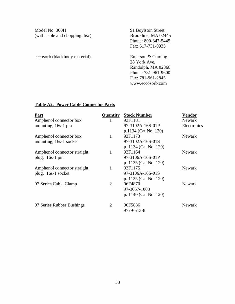
Model No. 300H (with cable and chopping disc)

91 Boylston Street Brookline, MA 02445 Phone: 800-347-5445 Fax: 617-731-0935

eccosorb (blackbody material) Emerson & Cuming 28 York Ave. Randolph, MA 02368 Phone: 781-961-9600 Fax: 781-961-2845 www.eccosorb.com

Table A2. Power Cable Connector Parts Part Quantity Stock Number Vendor Amphenol connector box mounting, 16s-1 pin

1 93F1181 97-3102A-16S-01P p.1134 (Cat No. 120)

Newark Electronics

Amphenol connector box mounting, 16s-1 socket

1 93F1173 97-3102A-16S-01S p. 1134 (Cat No. 120)

Newark

Amphenol connector straight plug, 16s-1 pin

1 93F1164 97-3106A-16S-01P p. 1135 (Cat No. 120)

Newark

Amphenol connector straight plug, 16s-1 socket

1 93F1175 97-3106A-16S-01S p. 1135 (Cat No. 120)

Newark

97 Series Cable Clamp

2 96F4870 97-3057-1008 p. 1140 (Cat No. 120)

Newark

97 Series Rubber Bushings

2 96F5886 9779-513-8

Newark

34

Table A3. Chassis Hardware, Receiver Part Quantity Stock Number Vendor Chassis box 17”x 11”x 5”

1

91F1340 Bud AC-422 p. 1927 (Cat No. 120)

Newark Electronics

BNC Female to Female chassis connector Isolated

2 39F3631 Pomona 3846 p. 1280 (Cat No. 120)

Newark

Terminal Strip 8-position

1 87F5241 Marathon Special Products 600-GP-8

Newark

Fan, 40 mm sq. x 10 mm, 12V DC

1 91F7442 Comair Rotron 032608(CR0412HB-G p. 531 (Cat No. 120)

Newark

Thermocouple, Type k

1 WT(K)-8-24 Cat. p. A-21

Omega

Thermocouple panel jack

1 RMJ-K-R Cat p. G-41

Omega

Miniature Connector 1

SMPW-K-(MF) Cat. p. G-14

Omega

SMA right angle connector, Male to male

2 PE9418 Cat. #2004S p. 164

Pasternack Enterprises

SMA right angle connector, Male to female

2 PE9068 Cat. #2004S p. 153

Pasternack

SMA (m) to BNC (f) adapter

1 PE9074 Cat. #2004S p.153

Pasternack

BNC cables 2

PE3067-12 50 ohm RG58 Cat #2004S p. 17

Pasternack

DIN Plug 1 84N1185 Voltrex SPC4101 p. 1333 (Cat No. 120)

Newark Electronics

DIN Receptacle

1

84N1184 Voltrex SPC4100 p. 1333 (Cat No. 120)

Newark

35

Table A4. Milliwave Power Supply Part Quantity Stock Number Vendor Power Supplies

15 V, 400 mA 12 V, 700 mA 15 V, 600 mA

1 1 1

Model No. 15EB40 Model No. 12EB70 Model No. 15EB60

Acopian Technical Company P.O. Box 638 Easton, PA 18044 Phone: 610-258-5441 Fax: 610-258-2842

Chassis Box 3” x 10” x 5”

1

90F947 Bud AC-404 p. 1927 (Cat No. 120)

Newark

Fan, 40 mm sq. x 10 mm, 12V DC

1 91F7442 Comair Rotron 032608(CR0412HB-G p. 531 (Cat No. 120)

Newark

Power cord Receptacle 1

98F1661 Volex, Inc. 17252A-B1-0 p. 877 (Cat No. 120)

Newark

Power cord

1

19C1624 SPC Technology SPC10288 p. 879 (Cat No. 120)

Newark

Fuse Holder

1 27F797 Littelfuse H342858 p. 928 (Cat No. 120)

Newark

Fuse 1

27F859 Littlefuse 312010 10A 250 V

Newark

Indicator light 1

93F3552 Chicago Miniature Lamp 1030D1 p. 491 (cat No. 120)

Newark

On/off switch

1

23F230 Eaton 7501K13 p. 678 (cat No. 120)

Newark

Heat Sinks 2 58F539 Newark

36

Wakefield Engineering 623K p.437 (Cat No. 120)

Rubber Feet 1

32828014 ½ x ½” p. 1870 (Cat 2000/2001)

MSC Industrial Supply