mike eco lab agent based modelling

MIKE 2017

MIKE ECO Lab – Agent Based Modelling

ABM Lab - Drifter Example

Step-by-step training guide

abm_stepbystep_1_drifterexample.docx/MPO/2017-09-12 - © DHI

DHI headquarters

Agern Allé 5

DK-2970 Hørsholm

Denmark

+45 4516 9200 Telephone

+45 4516 9333 Support

+45 4516 9292 Telefax

[email protected]

www.mikepoweredbydhi.com

i

CONTENTS

MIKE ECO Lab – Agent Based Modelling ABM Lab – Drifter Example Step-by-step training guide

1 Introduction ....................................................................................................................... 1 1.1 Background .......................................................................................................................................... 1 1.2 Objective .............................................................................................................................................. 1 1.3 ABM Examples ..................................................................................................................................... 2

2 Passive Drifter ................................................................................................................... 3 2.1 Purpose ................................................................................................................................................ 3 2.2 Files ...................................................................................................................................................... 3 2.3 Scenario ............................................................................................................................................... 4 2.4 Parameters ........................................................................................................................................... 5 2.4.1 Hydrodynamic parameters ................................................................................................................... 5 2.4.2 Sources ................................................................................................................................................ 5 2.4.3 Outputs ................................................................................................................................................. 5 2.5 Creating the Particle Class ‘Passive Drifter’ ........................................................................................ 6 2.5.1 Adding elements to address the flow information ................................................................................ 7 2.5.2 Creating a new particle class ............................................................................................................... 9 2.5.3 Creating class state variables ............................................................................................................ 10 2.5.4 Creating class constants .................................................................................................................... 11 2.5.5 Movement definition ........................................................................................................................... 11 2.5.6 Horizontal movement ......................................................................................................................... 11 2.5.7 Vertical movement ............................................................................................................................. 12 2.6 Model Setup of MIKE ECO Lab ......................................................................................................... 14 2.7 Loading a template ............................................................................................................................. 14 2.7.1 The Eulerian framework ..................................................................................................................... 14 2.7.2 Class overview ................................................................................................................................... 15 2.7.3 Specifying class constants ................................................................................................................. 15 2.7.4 Dispersion settings ............................................................................................................................. 16 2.7.5 Particle sources .................................................................................................................................. 16 2.7.6 Outputs mapping particle state variables into concentration maps ................................................... 19 2.7.7 Outputs storing particle movement tracks.......................................................................................... 23 2.7.8 Model setup of PT module ................................................................................................................. 24 2.8 Results ............................................................................................................................................... 26 2.8.1 Adjusting the track overlay ................................................................................................................. 28


ii ABM Lab - Drifter Example - © DHI

Introduction

1

1 Introduction

1.1 Background

Definition: ‘Models describing the (autonomic) behaviour and states of agents, objects or individuals’

Agent Based Modelling, in short ABM (or synonymously ‘Individual Based Modelling’,

IBM) is a relatively recent development. As Grimm and Railsback1 point out, ‘classical

theoretical ecology…usually ignores individuals and their adaptive behaviour’.

Ecosystems are commonly seen from a process based view, following the fate of masses

or concentrations in the system. Such process orientated modelling is done by describing

the flow between different components and the associated process. It is a well-

established and proven method and usually the first choice if you want to simulate

dissolved substances e.g. oxygen concentrations, BOD levels, pollutants or phyto- or

zooplankton distributions on a larger scale.

Many phenomena, however, cannot be described satisfactory using such process

orientated models. For example it is well known that plankton organisms that are subject

to passive transport by the water currents may show an explicit diel or diurnal2 vertical

migration through the water column. In the ocean this vertical migration can span over

several 100 m’s. By feeding at the surface and defecating large pellets in deeper zones

plankton organism can influence the transport of organic matter to deeper layers. If the

flow patterns are different throughout the water column such movement will also affect the

species distribution. ABMs can be used to describe and investigate such patterns by

reproducing the observed movement of individuals (agents) and the resulting changes to

the system.

The MIKE ECO Lab ABM module allows you to easily formulate agent based models

within the MIKE FM series of hydrodynamic environments of the MIKE Powered by DHI

framework. It combines the normal, process orientated MIKE ECO Lab framework with a

Lagrange particle movement model.

It is assumed that the reader is familiar with ‘classic’ process orientated modelling in MIKE

ECO Lab in the following text. In doubt consult the other MIKE ECO Lab manuals.

1.2 Objective

The objective of this Step-by-Step guide is to introduce the user to ABM modelling

techniques in MIKE ECO Lab and the various features/elements of an ABM template. A

series of examples are available; each designed to introduce the user to special features

of the modelling engine. A general understanding and experience with MIKE ECO Lab

and the MIKE FM series is expected. In doubt, consult the according manuals.

1 V. Grimm, S.F. Railsback; ‘Individual-based Modeling and Ecology’, Princeton University Press 2005

2 Many plankton organisms migrate to feed in the euphotic zone near the surface and rest in the mesopelagic zone

(or the hypolimnion in freshwater lakes) during a day cycle.


2 ABM Lab - Drifter Example - © DHI

The single examples are not directly related to each other but it is assumed that a user is

familiar with features introduced in previous chapters.

1.3 ABM Examples

The ABM Step-by-Step guide consists of a set of different examples for Agent based

modelling with MIKE ECO Lab, demonstrating various features of the MIKE ECO Lab

ABM Lab module. It is advised to explore them in the order listed below. Each example

introduces new features and options and assumes that the reader is familiar with the

previous ones.

The following examples are available.

Example Description

Passive Drifter General introduction, comparing a standard particle tracking with

a basic ABM template of a passive drifting agent

Vertical Movement A pelagic plankton organism moving vertically in the water

column triggered by local light intensity

Active Swimmer Active swimming agents in a tank, avoiding collisions with the

tank wall

The Swarm Active swimming agents forming a basic swarm

A description of the first example ‘Passive Drifter’ can be found in Section 2.

Passive Drifter

3

2 Passive Drifter

2.1 Purpose

This example introduces the basic agent template. It creates a passive drifting agent class

that is transported solely by the current. It has been designed to compare the results of

the standard particle tracking module with a passive drifting ABM particle class. It

demonstrates a very simple ABM model; nevertheless this simple passive drifting class

demonstrates how to distribute an ABM particle class according to the environmental flow

and this general movement is the base for almost all ABM particle classes.

Topics:

• Basic ABM features

• ABM state variables

• Movement vectors

• (Moving) point source

2.2 Files

The described example consists of the following files:

File Description

Corner.mesh Mesh file containing the environment definition

(bathymetry, land, etc.)

Corner2D_HD.m21fm Basic hydrodynamic setup for MIKE 21 FM

PassiveDrifter.ecolab The final template for the described ‘Passive Drifter’

ABM particle class

Source_Location.dfs0 A time series with coordinates for the moving source

coordinate definition

Compare_Corner_PT_ABM.m21fm

Compare_Corner_PT_ABM.m3fm

The final MIKE FM setup to compare the ABM and

classic particle tracking



2.3 Scenario

We want to follow the drift of individuals of a passive drifting ABM particle class. The

model uses the same L-shaped channel with a constant depth as the introduction

example in the particle tracking. The computational domain is shown in Figure 2.1.

• The channel is about 500 wide, with 1 km stretch on either side of the corner. The

bottom is 20 m below datum.

• The flow goes from south to west with a current of approximately 0.8 m/s caused by

a water level difference of 0.05 m between the open boundaries.

• Particles are released by a moving point source starting at the position (1250, 200),

moving towards (1400, 200) at a depth of -5.04 m.

Figure 2.1 Model domain for the comparison of standard particle tracking and a passive drifting

ABM particle class

Passive Drifter

5

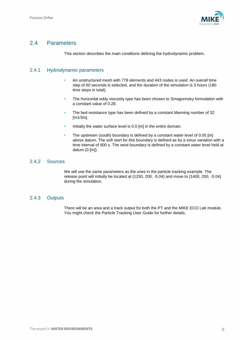
2.4 Parameters

This section describes the main conditions defining the hydrodynamic problem.

2.4.1 Hydrodynamic parameters

• An unstructured mesh with 778 elements and 443 nodes is used. An overall time

step of 60 seconds is selected, and the duration of the simulation is 3 hours (180

time steps in total).

• The horizontal eddy viscosity type has been chosen to Smagorinsky formulation with

a constant value of 0.28.

• The bed resistance type has been defined by a constant Manning number of 32

[m1/3/s].

• Initially the water surface level is 0.0 [m] in the entire domain.

• The upstream (south) boundary is defined by a constant water level of 0.05 [m]

above datum. The soft start for this boundary is defined as by a sinus variation with a

time interval of 900 s. The west boundary is defined by a constant water level held at

datum (0 [m]).

2.4.2 Sources

We will use the same parameters as the ones in the particle tracking example. The

release point will initially be located at (1250, 200, -5.04) and move to (1400, 200, -5.04)

during the simulation.

2.4.3 Outputs

There will be an area and a track output for both the PT and the MIKE ECO Lab module.

You might check the Particle Tracking User Guide for further details.



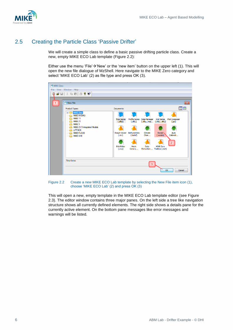
2.5 Creating the Particle Class ‘Passive Drifter’

We will create a simple class to define a basic passive drifting particle class. Create a

new, empty MIKE ECO Lab template (Figure 2.2):

Either use the menu ‘File’‘New’ or the ‘new item’ button on the upper left (1). This will

open the new file dialogue of MzShell. Here navigate to the MIKE Zero category and

select ‘MIKE ECO Lab’ (2) as file type and press OK (3).

Figure 2.2 Create a new MIKE ECO Lab template by selecting the New File item icon (1),

choose ‘MIKE ECO Lab’ (2) and press OK (3)

This will open a new, empty template in the MIKE ECO Lab template editor (see Figure

2.3). The editor window contains three major panes. On the left side a tree like navigation

structure shows all currently defined elements. The right side shows a details pane for the

currently active element. On the bottom pane messages like error messages and

warnings will be listed.

Passive Drifter

7

Figure 2.3 A new, empty MIKE ECO Lab template in the template editor. Provide a proper

description (1) and enable the ABM features (2).

When you create a new template the general information page will be active and you can

provide a short description (1) and links to more detailed documentation for the current

template. If you want to define an ABM template enable the appropriate checkbox (2).

This will add the ‘Particle Classes’ to the navigation tree. It is a good idea to save the new

template as ‘PassiveDrifter’.

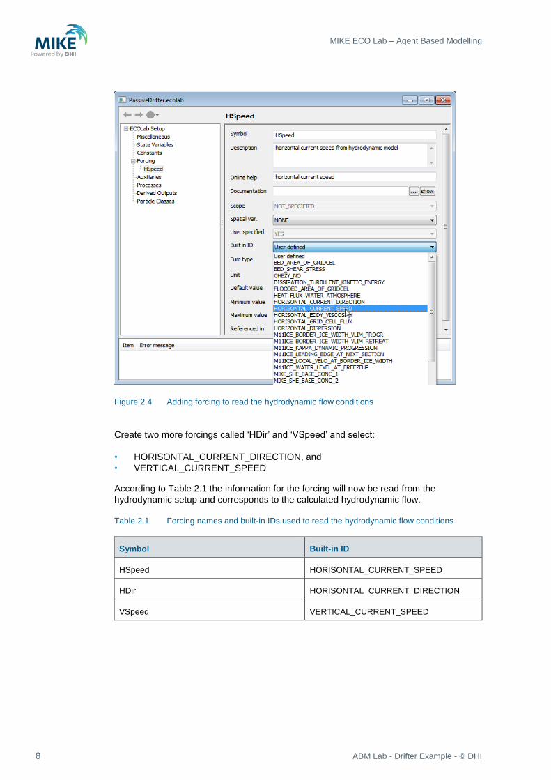
2.5.1 Adding elements to address the flow information

Most ABM templates will need to address the flow field to move agents with the currents.

The flow information is part of the Eulerian framework and is usually declared as a

forcing. To create a new forcing use the context menu (right mouse button) in the left

navigation pane inside the node labelled ‘Forcing’ and select ‘Create new’. This will add a

new forcing and open the details page for the new created element. Name it ‘HSpeed’

and provide information for description and the online help. To query the flow field from

the hydrodynamic model select the built-in ID ‘HORIZONTAL_CURRENT_SPEED’ from

the list of available built-in forcing. By selecting a built-in ID all necessary information for

the other fields is set automatically. See Figure 2.4.



Figure 2.4 Adding forcing to read the hydrodynamic flow conditions

Create two more forcings called ‘HDir’ and ‘VSpeed’ and select:

• HORISONTAL_CURRENT_DIRECTION, and

• VERTICAL_CURRENT_SPEED

According to Table 2.1 the information for the forcing will now be read from the

hydrodynamic setup and corresponds to the calculated hydrodynamic flow.

Table 2.1 Forcing names and built-in IDs used to read the hydrodynamic flow conditions

Symbol Built-in ID

HSpeed HORISONTAL_CURRENT_SPEED

HDir HORISONTAL_CURRENT_DIRECTION

VSpeed VERTICAL_CURRENT_SPEED

Passive Drifter

9

2.5.2 Creating a new particle class

To create a new particle class activate the ‘Particle classes’ node in the navigation tree.

This will open the details page for the particle classes. As up to now no particle class

have been declared the page is empty.

The shown list is a generic element, available for all MIKE ECO Lab element categories.

Elements in such a list can be added, removed (if not referenced) and moved up and

down with the buttons in the upper right side. On the upper left side a chronic navigation

toolbar allows you to quickly jump back and fore between already visited elements.

Compare Figure 2.5.

Figure 2.5 Creating a new particle class using the ‘New’ button

Use the ‘New’ button to create a new particle class with the default name ‘Specie_1’.

Rename it to ‘PassiveDrifter’ by changing its symbol name on the overview page. A new

created particle class will not have any internal state variables, constants or arithmetic

expressions but it has always at least one horizontal movement vector and a downward

movement velocity definition.

Figure 2.6 New created particle class with no variables



2.5.3 Creating class state variables

To be able to store some data like a particle mass and derive a concentration map from

the particle distribution we add a simple state variable to the particle class.

You can use either the context menu on the ‘State Variables’ node in the ‘Particle classes’

section, or the ‘New’ button in the particle state variable list to do so.

First, you have to provide a symbol/variable name. This name will be used to address the

value represented by the state variable in later MIKE ECO Lab expressions.

You should provide a good, catchy description text. This description will be used as

annotation in the result files/plots and to identify the variable in the setup interface!

Therefore it is good practise to repeat the symbol name together with a short description

here. Lengthy documentations should be placed in an external file, linked to the

‘documentation’ field.

Furthermore, you can specify a EUM type3 from a list of predefined options. This will set

the item unit; if no proper predefined EUM type is available, select ‘User defined’ and

specify the unit manually. Please note that MIKE ECO Lab does not handle unit

conversions automatically – you have to ensure that any calculation is done with the

proper unit!

Do not forget to provide meaningful data for default, min and max values as this

information will be used to validate the input data!

Finally, your input should look like the input shown in Figure 2.7.

Figure 2.7 Create a simple conservative state variable for the particle class; make sure that the

process expression (rate of change) is ‘0’

3 EUM stands for ‘Engineering Unit Management’ and is the internal technique used for automatic unit conversion inside

the MIKE products.

Passive Drifter

11

2.5.4 Creating class constants

Now create a new constant. This constant will specify the settling velocity of our particle

class. Name it ‘settling_v’, set the unit to ‘m/s’. Specify ‘0’ as default value (no settling)

and allow a minimum of ‘-10.0’ and a maximum of ‘10.0’. This will enable us to assign

positive and negative buoyancy to a particle. See Figure 2.8 for details.

Figure 2.8 Definition of a constant used as settling velocity

2.5.5 Movement definition

Now we need to declare the movement rules of the simple particle class. An ABM

particle/agent in MIKE ECO Lab can have up to 5 independent horizontal movement

vectors and has one downward (settling) velocity. In this example we will specify the

current flow direction and speeds that we have created as forcing in the first step. This will

cause an individual from the particle class to be passively dispersed by the currents

(through advection).

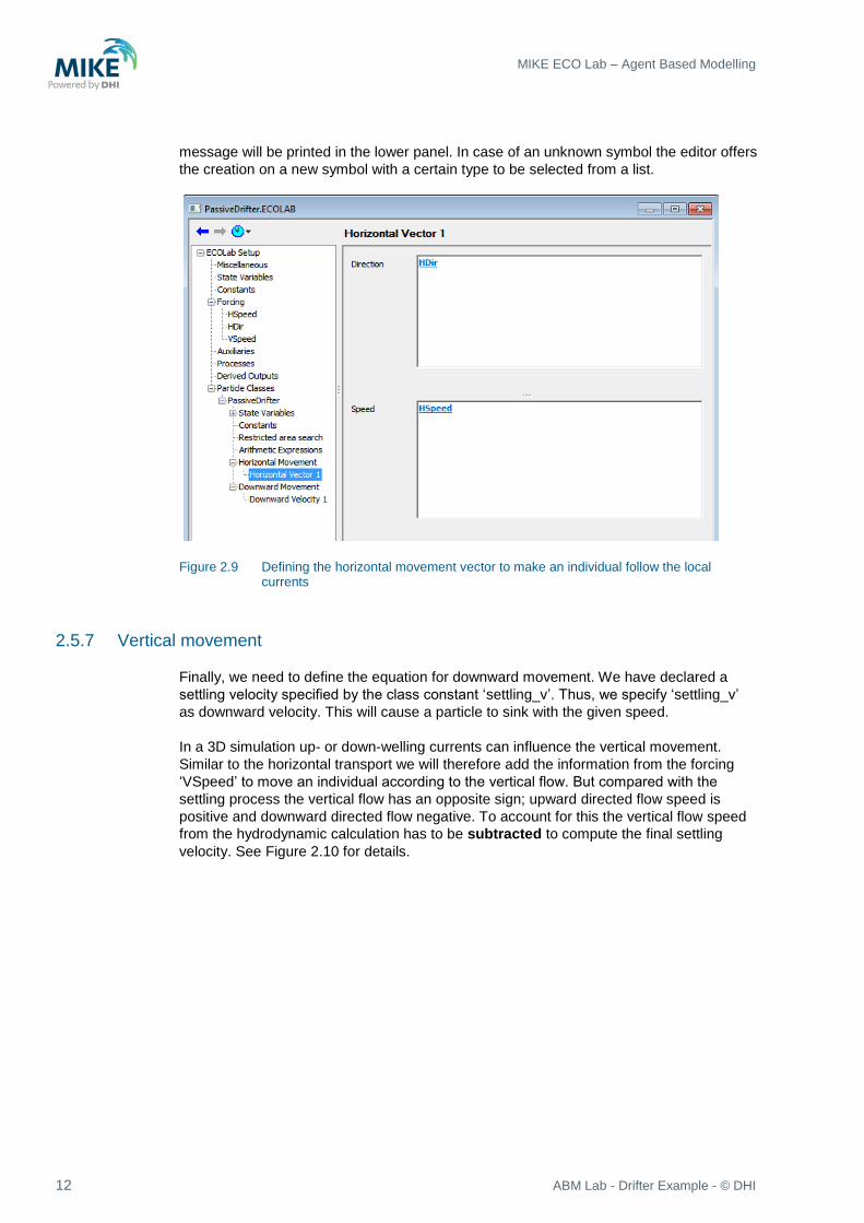
2.5.6 Horizontal movement

To do so open the first horizontal movement vector definition. We will use the horizontal

flow speed and direction information to move an individual horizontally with the current

flow. Enter the symbol name used for the current speed and direction in the

corresponding fields (see Figure 2.9).

The expression you enter is checked/ verified when you move to another input field. If the

editor recognises the entered symbol as previously defined, the text becomes blue with

an underscore. This indicates a hyperlink and you can navigate to the definition (~input

dialogue) of the element/symbol by using the right mouse button. In case of an error a



message will be printed in the lower panel. In case of an unknown symbol the editor offers

the creation on a new symbol with a certain type to be selected from a list.

Figure 2.9 Defining the horizontal movement vector to make an individual follow the local

currents

2.5.7 Vertical movement

Finally, we need to define the equation for downward movement. We have declared a

settling velocity specified by the class constant ‘settling_v’. Thus, we specify ‘settling_v’

as downward velocity. This will cause a particle to sink with the given speed.

In a 3D simulation up- or down-welling currents can influence the vertical movement.

Similar to the horizontal transport we will therefore add the information from the forcing

‘VSpeed’ to move an individual according to the vertical flow. But compared with the

settling process the vertical flow has an opposite sign; upward directed flow speed is

positive and downward directed flow negative. To account for this the vertical flow speed

from the hydrodynamic calculation has to be subtracted to compute the final settling

velocity. See Figure 2.10 for details.

Passive Drifter

13

Figure 2.10 Defining the settlement of the particle class. See text why the vertical flow speed

needs to be subtracted

ATTENTION: The forcing ‘VSpeed’ refers to the vertical current speed. The coordinate system

for the current flow points upwards, meaning a negative flow speed indicates a downward

direction whereas a positive value shows an upward directed flow. The vertical movement of a

particle expects a downward velocity, i.e. a positive downward velocity causes a downward

movement whereas a negative value indicates positive buoyancy and an upward movement.

Thus the sign of ‘VSpeed’ needs to be negated to move a particle according to the vertical

current flow.

Save the final template. It can now be used in a hydrodynamic setup.



2.6 Model Setup of MIKE ECO Lab

Open the hydrodynamic setup ‘Corner_2D_HD.m21fm’4. This contains the basic

hydrodynamic setup for the simple ABM example. Save the setup to a new file name

‘Compare_Corner_PT_ABM.m21fm’ to not overwrite the existing setup. Enable both the

PT and the ‘MIKE ECO Lab / Oilspill’ modules on the ‘Module Selection’ page.

2.7 Loading a template

Now load the ABM template for the passive drifting particle class you have created. Open

the ‘Model Definition’ page, select ‘From File’ and pick the MIKE ECO Lab template

containing the ‘PassiveDrifter’ particle class form your disc. If successful loaded you

should see that the summary lists one particle class and three forcing. Inspect the

overview (compare Figure 2.11).

Figure 2.11 Setup overview, conservative state variable

2.7.1 The Eulerian framework

The Eulerian framework represents concentration type state variables, constants and

forcing. Make sure that all utilised built-in constants and forcing are correctly handled; if

the hydrodynamic engine cannot provide the proper information, the user has to supply

the missing data! For further reference see the standard MIKE ECO Lab User Guide.

4 If the file is not available on your disc you can create a new setup using the specifications from 2.4

Passive Drifter

15

2.7.2 Class overview

The ‘Classes’ node allows you to inspect all defined particle classes. In our small example

we have just defined one class (see Figure 2.12). The ‘State Variables’ node allows you

to get an overview of the state variables defined by the active class. As every individual

agent/particle has an own set of state variables, the presented information just includes

the name and unit of the variables. Initial values of state variables have to be specified

when particles are created, i.e. in the source definitions (see Particle sources, page 16).

Figure 2.12 Overview of all defined particle classes

2.7.3 Specifying class constants

The value(s) of particle class constants are valid for all individuals of a particle class. They

have to be specified in the ‘Constants’ node under the ‘Classes’ overview node.

In our example we use a class constant to specify the settling velocity. To modify the

default value, move to the ‘Constants’ of the class (see Figure 2.13). Here, all the defined

constants are listed and the user can set specific numeric values for the single class

constants. Specify a settling velocity of -1.4e-3 m/s. this will cause a slight positive buoyant

particle, moving upward from the release depth (-5.04 m) to the surface in one hour.

Figure 2.13 Parameterisation of class constants



2.7.4 Dispersion settings

We have declared the movement vector for our particle class in the template and

specified the flow components as the sole driver in the movement definition. The created

particle class is a simple passive drifting agent it simply moves with the local current flow.

If you want to add a random element (random walk) to the movement of an ABM

agent/particle class it is easiest to use the built-in functionality of the hydrodynamic

module5 via the dispersion settings. For details check the topic in the standard Particle

Tracking User Guide.

To specify the dispersion settings for a particle class move to the ‘Dispersion’ node. In our

example use ‘Scaled Eddy viscosity formulation’ for horizontal dispersion and ‘no

dispersion’ for vertical dispersion (see Figure 2.14)

Figure 2.14 Horizontal dispersion settings

2.7.5 Particle sources

If particles/agents are not dynamically created, they must ‘enter’ a simulation using a

particle source. A particle sources is defined as a spatial location where new particles can

be introduced to the mode domain. You can specify the number of particles released

within one time step and the initial values of their state variables. As particle constants

cannot vary during the simulation time they have to be configured globally (see Creating

class constants, page 11).

MIKE ECO Lab offers two principally different source types. ‘Point sources’ represent

single point locations whereas ‘Area sources’ can describe spatial regions, where new

particles are placed. Both types have subtypes; point sources can be stationary or moving

5 You can also implement an additional random walk as a movement vector in the EOC Lab template.

Passive Drifter

17

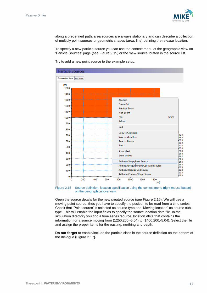
along a predefined path, area sources are always stationary and can describe a collection

of multiply point sources or geometric shapes (area, line) defining the release location.

To specify a new particle source you can use the context menu of the geographic view on

‘Particle Sources’ page (see Figure 2.15) or the ‘new source’ button in the source list.

Try to add a new point source to the example setup.

Figure 2.15 Source definition, location specification using the context menu (right mouse button)

on the geographical overview.

Open the source details for the new created source (see Figure 2.16). We will use a

moving point source, thus you have to specify the position to be read from a time series.

Check that ‘Point source’ is selected as source type and ‘Moving location’ as source sub-

type. This will enable the input fields to specify the source location data file. In the

simulation directory you find a time series ‘source_location.dfs0’ that contains the

information for a source moving from (1250,200,-5.04) to (1400,200,-5.04). Select the file

and assign the proper items for the easting, northing and depth.

Do not forget to enable/include the particle class in the source definition on the bottom of

the dialogue (Figure 2.17).



Figure 2.16 Moving source definition

Figure 2.17 Do not forget to enable/include the particle class in source definition!

Now you have to configure the number of released particles per time step and the initial

value of the state variable for these particles. Specify the number of released particles as

1 per time step. The dialogue will list all defined state variables and the currently chosen

initial value. To modify the initial value jump the state variable dialogue using the ‘Edit’

button.

If the state variable is defined to be a mass (defined by the EUM type when you set up the

template!) you can specify a total released amount that is distributed among all released

particles. This is very useful if you want to adjust the number of release particles (as

otherwise you have to recalculate the state variable amounts when you change to number

of released particles). Further it is possible to set a flag that the specified value is actually

Passive Drifter

19

a flux per second. Using that option the total amount will not change if you change the

time step. See Figure 2.18 for actual settings.

Figure 2.18 Source definition, specification of released particles and settings

2.7.6 Outputs mapping particle state variables into concentration maps

We will create two principally different types of outputs, one map output and a particle

track output. The latter is a XML data file containing the information on individual particles

(their position, state variables and properties) whereas the map file is a spatial

representation where state variables from all particles are mapped spatially as a

concentration map.

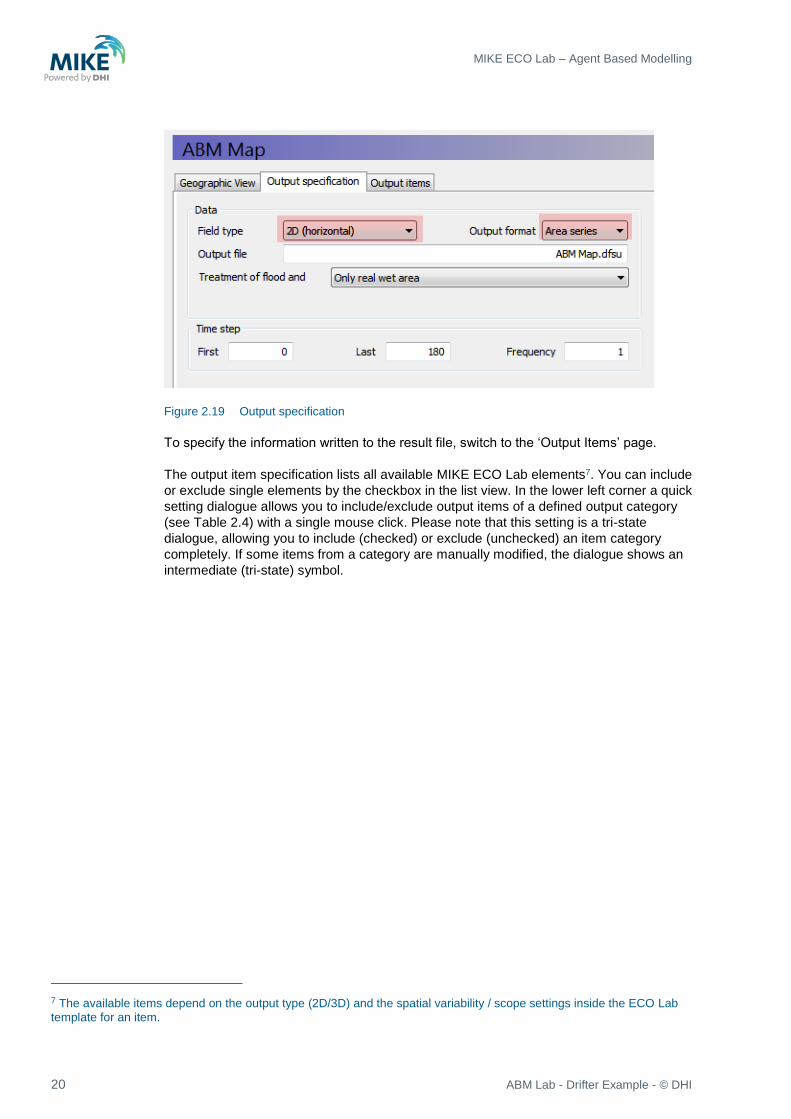
Create two new output files and name the first ‘ABM Map’ and the last ‘ABM Track’. Open

the specification for the ‘ABM Map’. As ‘Field type’ select ‘2D (horizontal)’, set the output

format to ‘Area series’. Provide a proper file name (‘ABM_Map.dfsu’6). For simplicity

reason we will include all time steps and use an output frequency of 1. See Figure 2.19.

6 If you change the output format and move away from the input field the proper file extension will be set for the file name!



Figure 2.19 Output specification

To specify the information written to the result file, switch to the ‘Output Items’ page.

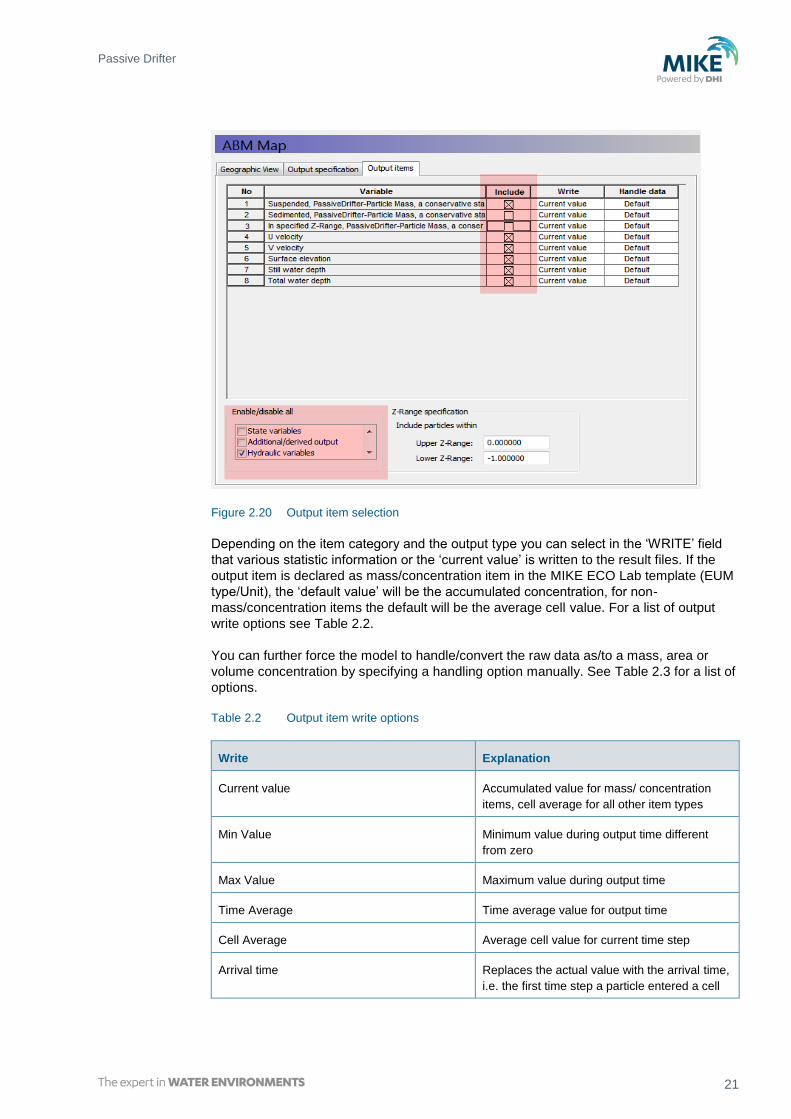
The output item specification lists all available MIKE ECO Lab elements7. You can include

or exclude single elements by the checkbox in the list view. In the lower left corner a quick

setting dialogue allows you to include/exclude output items of a defined output category

(see Table 2.4) with a single mouse click. Please note that this setting is a tri-state

dialogue, allowing you to include (checked) or exclude (unchecked) an item category

completely. If some items from a category are manually modified, the dialogue shows an

intermediate (tri-state) symbol.

7 The available items depend on the output type (2D/3D) and the spatial variability / scope settings inside the ECO Lab

template for an item.

Passive Drifter

21

Figure 2.20 Output item selection

Depending on the item category and the output type you can select in the ‘WRITE’ field

that various statistic information or the ‘current value’ is written to the result files. If the

output item is declared as mass/concentration item in the MIKE ECO Lab template (EUM

type/Unit), the ‘default value’ will be the accumulated concentration, for non-

mass/concentration items the default will be the average cell value. For a list of output

write options see Table 2.2.

You can further force the model to handle/convert the raw data as/to a mass, area or

volume concentration by specifying a handling option manually. See Table 2.3 for a list of

options.

Table 2.2 Output item write options

Write Explanation

Current value Accumulated value for mass/ concentration

items, cell average for all other item types

Min Value Minimum value during output time different

from zero

Max Value Maximum value during output time

Time Average Time average value for output time

Cell Average Average cell value for current time step

Arrival time Replaces the actual value with the arrival time,

i.e. the first time step a particle entered a cell



Please note that an item can just appear once in the output file. It is not possible to write

the min and max value to the same output file.

Table 2.3 Output item handling options

Handle data Explanation

Default Accumulated value for mass/ concentration

items, cell average for all other item types

As mass Accumulated value

As area concentration Accumulated value divided by element area

As volume concentration Accumulated value divided by element

volume

Table 2.4 Output item categories for map outputs

Category Explanation

State variables MIKE ECO Lab state variables from the

Eulerian framework (concentration variables)

Additional/ derived outputs Auxiliary variables, process and derived

outputs from the Eulerian framework

Hydraulic variables Information from the hydrodynamic core, e.g.

current information etc.

Suspended state variables State variables from suspended particles

mapped as concentrations

Suspended derived outputs Arithmetic expressions from suspended

particles mapped as concentrations

Sedimented state variables State variables from sedimented particles

(based on sedimentation flag) mapped as

concentrations

Sedimented derived outputs Arithmetic expressions from sedimented

(based on sedimentation flag) particles

mapped as concentrations

z-range state variables State variables from particles within the

specified Z-range mapped as concentrations

z-range derived outputs Arithmetic expressions from particles within

the specified Z-range mapped as

concentrations

Passive Drifter

23

2.7.7 Outputs storing particle movement tracks

The second output is used to store the particle track, the detailed information on particle

positions, state variables etc. as a XML file.

Set the output field type to ‘Particle Track’ and include all time steps and particles (see

Figure 2.21). By default the track will be stored as compressed particle track. This

compressed format reduces the memory constrains of the track file on the disc. If you

plan to post-process track data using 3rd party tools it is advised to store the information

‘uncompressed’ 8.

Figure 2.21 Particle track specification

Open the output item page and select the outputs to be included in the track result file.

The particle position (x, y, z coordinates) is always stored and additional items can be

included / excluded. There is a similar quick-selector as in the map output but as the track

stores different information the categories are slightly different (see Table 2.5)

8 Check the ECO Lab User Guide for a detailed format description of the XML file



Table 2.5 output categories for particle tracks

Category Explanation

State variables Particle state variables

Additional/ derived outputs Arithmetic expressions

Properties Particle properties

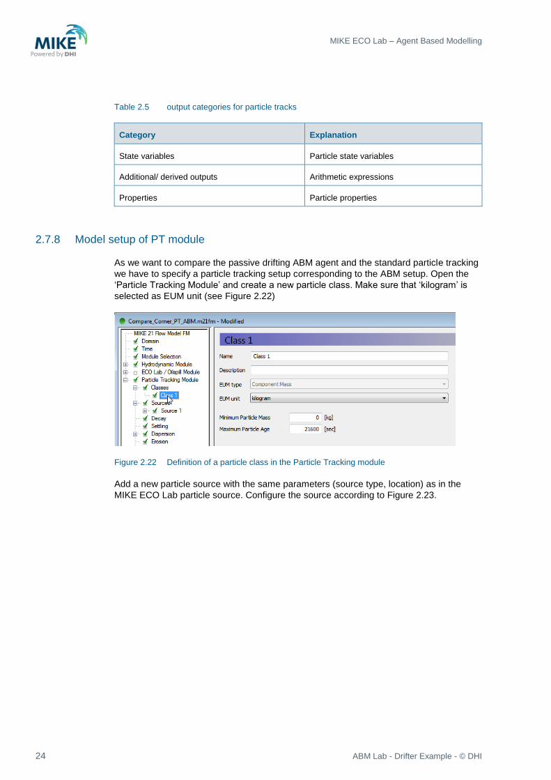
2.7.8 Model setup of PT module

As we want to compare the passive drifting ABM agent and the standard particle tracking

we have to specify a particle tracking setup corresponding to the ABM setup. Open the

‘Particle Tracking Module’ and create a new particle class. Make sure that ‘kilogram’ is

selected as EUM unit (see Figure 2.22)

Figure 2.22 Definition of a particle class in the Particle Tracking module

Add a new particle source with the same parameters (source type, location) as in the

MIKE ECO Lab particle source. Configure the source according to Figure 2.23.

Passive Drifter

25

Figure 2.23 Definition of the source in the Particle Tracking module

Set up two outputs: one as 2D output, the other as track output, analogous to the outputs

in the MIKE ECO Lab module (NOTE: the particle tracking module does not provide the

same output features as the MIKE ECO Lab ABM module).



2.8 Results

After you have run the model you can inspect the simulation results. Open the

‘concentration’ map form the MIKE ECO Lab module. This result type shows the particle

distribution based on a mapping of the particle state variables into concentrations. This

result type is not different from any other MIKE result.

Figure 2.24 Resulting concentration map output for the particle class after 65 time steps

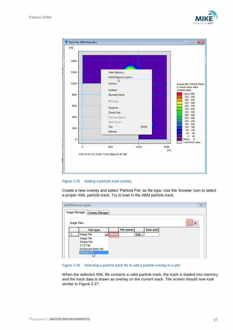
To display the information stored as the particle track you have to add a particle overlay to

the result display. Use the context menu on the display area and select ‘Add/Remove

Layers’ (see Figure 2.25)

Passive Drifter

27

Figure 2.25 Adding a particle track overlay

Create a new overlay and select ‘Particle File’ as file type. Use the ‘browse’ icon to select

a proper XML particle track. Try to load in the ABM particle track.

Figure 2.26 Selecting a particle track file to add a particle overlay to a plot

When the selected XML file contains a valid particle track, the track is loaded into memory

and the track data is drawn as overlay on the current track. The screen should now look

similar to Figure 2.27.



Figure 2.27 Loaded particle track overlay

The default track overlay shows the path of all particles drawn as white lines from their

origin to the end of the simulation. Particles are represented as geometric

shapes/markers and their colour represents the particles z-coordinate.

2.8.1 Adjusting the track overlay

A particle track overlay can be adjusted in many ways. Use the ‘Edit’ button in the

‘Add/Remove Layer’ dialogue. The first option ‘Particle Track Overlay’ (see Figure 2.28)

allows you to modify the lines drawn to represent the particle path according to the

specified line width, style and colour. The ‘Track length’ allows you to specify that the path

shows all time steps (‘Total’), just to the current time step (path from release location to

current location) or just the last n positions/time steps (‘Current with tail’).

Passive Drifter

29

Figure 2.28 Particle track overlay dialogue

The instantaneous overlay specifies the drawing of the shapes. You can specify any track

item used to control the colour and size of a symbol, as well as select a symbol shape.

Figure 2.29 Particle track instantaneous overlay

Common visualisation options:

Change the size of a marker according to a variable: • Select the output variable to control the size as ‘Marker size variable’

• Set ‘Marker size type’ to ‘variable’

• Set a scaling factor ‘Marker size’

Change the colour of a marker to match a variable: • Set the control variable ‘Marker color variable’

• Set ‘Marker fill style’ to ‘Palette color’



Apply a uniform maker colour: • Select colour ‘Marker color’

• Set ‘Marker fill style’ to ‘Solid color’ for a filled marker ‘White’ to draw a white shape

with colour border

• ‘Transparent’ to draw just the colour border

Now we can do a comparison of the final results. Add another overlay for the particle track

from the particle tracking module (2D concentration mapping is based on the results of

the ABM model and will not show the particles from the PT module!). Adjust the colours

and styles of the two overlays to be able to separate them visually. Use the ‘current with

tail’ option to draw the particles trajectories. The final plot should look similar to Figure

2.30.

When you compare the traces, both the passive drifting ABM particle class and the

standard particle tracking produce comparable tracks. The individual tracks are slightly

different as there is a random walk contribution due to the dispersion settings. If you

switch off horizontal dispersion for both MIKE ECO Lab and the particle tracking module

you will see that the tracks from both modules will be identical.

Why use an MIKE ECO Lab ABM then? We have not specified any decay for the state

variable but it is now quite simple to add e.g. a decay process. Thus you can easily apply

any decay function (1st order, 2nd order, dependent on light or other inhibition function etc.)

with a functionality the classic particle tracking does not allow. Further you can enhance

the movement rules to simulate ‘biological’ behaviour. We will explore these opportunities

in the next chapters.

Figure 2.30 Final results comparing MIKE ECO Lab ABM a track (while, square markers) and a

standard particle tracking (red, dotted path, filled circle markers) with the same properties

mike eco lab agent based modelling

Documents