migration resolution - king abdullah university of science ... · pdf file52 chapter 3....

Chapter 3

Migration Resolution

In this section time migration is defined and its pitfalls and benefits are compared to depthmigration. In the far-field approximation the resolution formula for analyzing a migrationimage is derived and its application to practical problems is analyzed.

3.1 Time Migration vs Depth Migration

Depth migration in a variable velocity medium can be effected by replacing the t = r/cstatement in the MATLAB script by the traveltime obtained from ray tracing seismic en-ergy from the trace position to the migrated image point. This is the correct procedurefor downward continuing recorded energy to its place of origin, and such traveltimes cancomputed by a finite-difference solution to the eikonal equation.

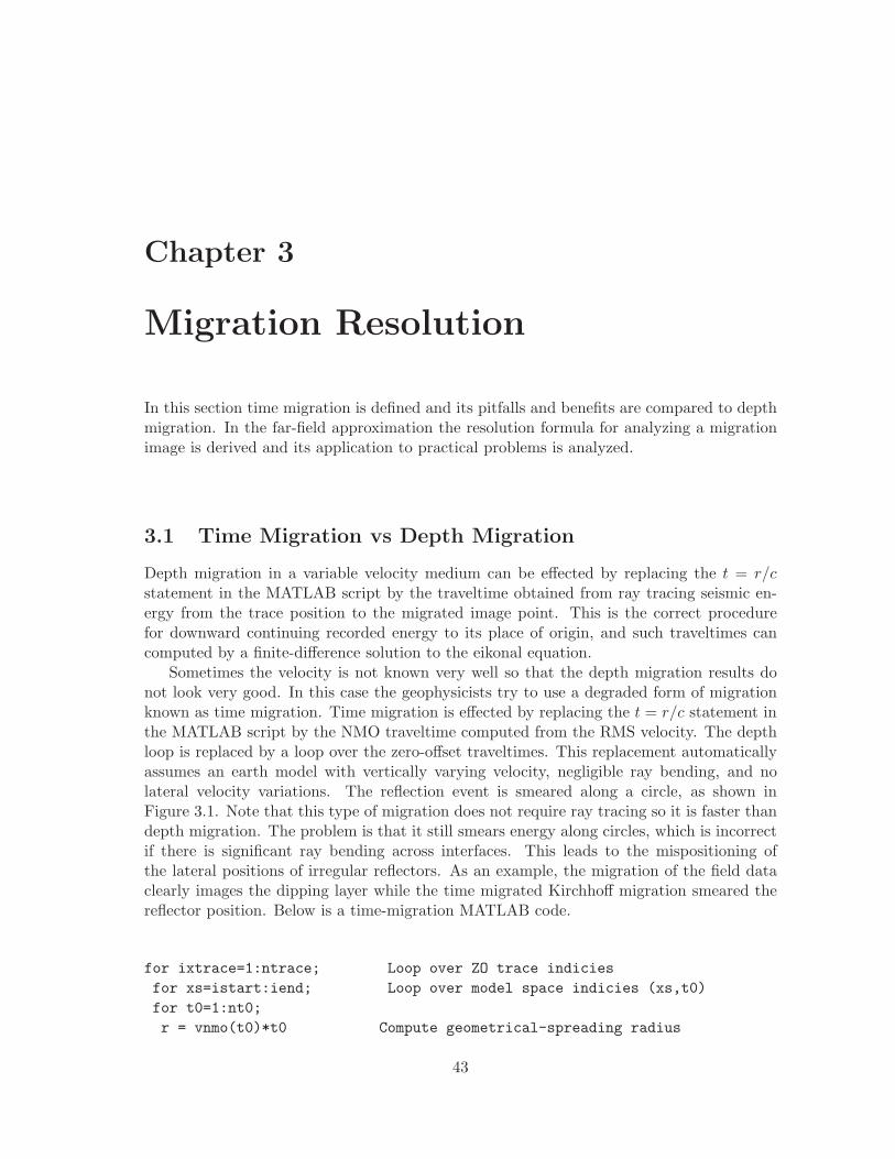
Sometimes the velocity is not known very well so that the depth migration results donot look very good. In this case the geophysicists try to use a degraded form of migrationknown as time migration. Time migration is effected by replacing the t = r/c statement inthe MATLAB script by the NMO traveltime computed from the RMS velocity. The depthloop is replaced by a loop over the zero-offset traveltimes. This replacement automaticallyassumes an earth model with vertically varying velocity, negligible ray bending, and nolateral velocity variations. The reflection event is smeared along a circle, as shown inFigure 3.1. Note that this type of migration does not require ray tracing so it is faster thandepth migration. The problem is that it still smears energy along circles, which is incorrectif there is significant ray bending across interfaces. This leads to the mispositioning ofthe lateral positions of irregular reflectors. As an example, the migration of the field dataclearly images the dipping layer while the time migrated Kirchhoff migration smeared thereflector position. Below is a time-migration MATLAB code.

for ixtrace=1:ntrace; Loop over ZO trace indicies

for xs=istart:iend; Loop over model space indicies (xs,t0)

for t0=1:nt0;

r = vnmo(t0)*t0 Compute geometrical-spreading radius

43

44 CHAPTER 3. MIGRATION RESOLUTION

time = sqrt( (t0/dt)^2 + (x/vnmo(t0)/dt)^2 ); Compute 1-way time to circle

m(xs,t0) = m(xs,t0) + data(ixtrace,time)/r; Smear/sum reflections into (x,t0)

end;

end;

end

One effect of time migration is that the time migration images sometimes looks betterthan depth migration images. This is because the images are plotted in offset vs two-wayvertical time space, so there will be no wavelet stretch due to a faster velocity medium. Thatis, in depth migration the wavelet is smeared within the fat semicircle, but if the velocity ofthe semicircle is faster at depth (longer wavelength for a given period) then the upper partof donut is thin and lower part of donut is fat. Compare the stretching effect in Figure 2.6to the no-stretch time migration section in Figure 2.7. Thankfully, time migration lookslike it is becoming less common because of the inaccuracies in positioning events.

However, time migration is preferred if the velocity model is not very well known. Why?Because the NMO velocity is obtained by looking for the best hyperbola that most coher-ently stacks reflections. Thus, time migration focuses energy as well as any summationalong hyperbolas can hope to achieve. Compare this to depth migration with a crummyvelocity model. For a crummy velocity model we are summing energy along a correspond-ingly crummy quasi-hyperbola, resulting in a crummy focused image. Crumbs in, crumbsout.

3.2 Spatial Resolution

What is the minimum separation between two point scatterers that can be resolved in amigrated section? This minimum distance is known as the spatial resolution of the migratedsection, where the horizontal resolution will differ from the vertical resolution. The spatialresolution will largely be a function of the wavelength λ, recording aperture L and/or depthof the scatterer.

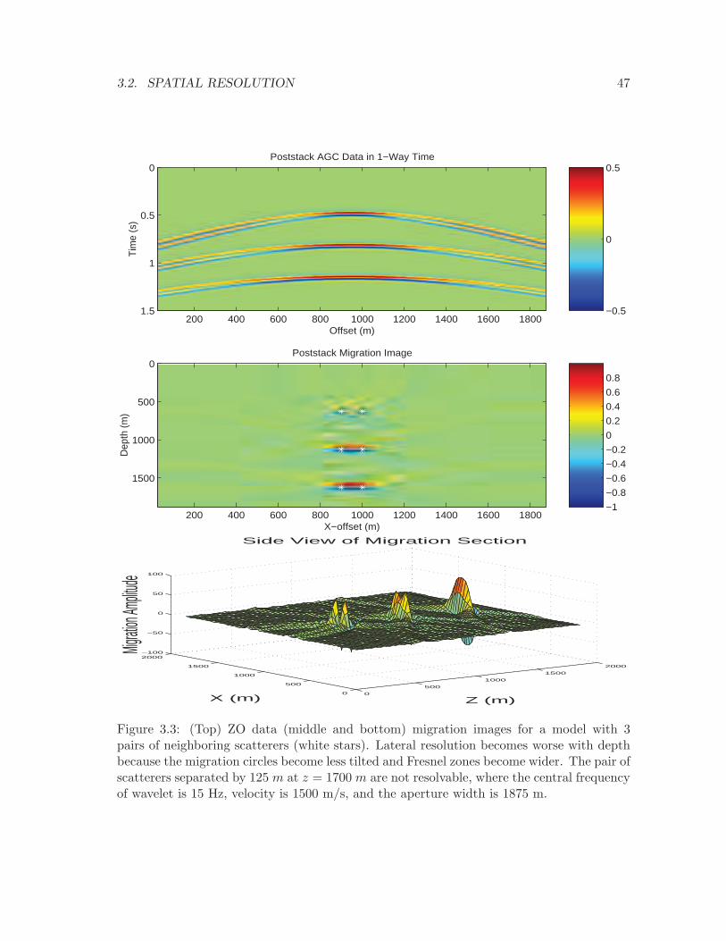
The spatial resolution is quantitatively estimated by using the idea of a Fresnel zone(Elmore and Heald, 1969), where the first Fresnel zones makes the largest contribution tothe recorded reflection signal, with a negligible contribution from the higher-order Fresnelzones. The definition of the 1st reflection Fresnel zone is the area on the reflector such thatany reflection ray path (see Figure 3.5) from source-to-reflector-geophone differs in totalpath length by no more than a λ/2 (or arrival time difference of T/2). Therefore, two pointscatterers located within each others first Fresnel zone will not be clearly distinguishablefrom one another on a migrated section because of interference effects. An example of imag-ing data for several neighboring point scatterers at different depths is given in Figure 3.3.Here, the lateral resolution becomes worse with depth because the migration circles becomeflatter with depth, so that the deepest pair of scatterers is not resolvable in the migration

3.2. SPATIAL RESOLUTION 45

T=3s

T=3s

Single ZO Trace

Time Migration Operator Depth Migration Operator

Figure 3.1: ZO time migration circles do not take into account raybending effects, so theresult is that time migration laterally mispositions the events. Depth migration takes intoaccount raybending across interfaces as well as lateral velocity variations, and so will cor-rectly image the ZO reflection energy. The problem is that the ZO trace is formed bystacking CMP traces using a 1D NMO formula, which can be inappropriate for earth mod-els with strong lateral velocity variations. The solution is prestack depth migration


Where is the Scatterer?

Answer: Here

1 2

2

Near−offset traces = better dz

Far−offset traces = better dx

1

Figure 3.2: Where is the scatterer located that explains the reflections in the near- and far-offset ZO traces? Answer: The quadrilateral intersection zone. The width of the intersectionzone is controlled by the far-offset (i.e., farthest from the scatterer) trace while its height iscontrolled by the near-offset (i.e., nearest to scatterer) trace.

image. The migration ellipses interfere such that only one bump rather than two appear inthe sideview image (Schuster, 1996; Chen and Schuster, 1999).

An intuitive picture of resolution limits is given in Figure 3.2. Here, two traces areused to resolve the location of a scatterer, where the intersection of the migration donutsdetermines the approximate location of the point scatterer. Note, the width (i.e., horizontalresolution limit) of the intersection zone is controlled by the width of the far-trace donut atthe scatterer point, while vertical height (i.e., vertical resolution limit) of the intersectionzone is controlled by the thickness of the near-trace donut at the scatterer point. Moregenerally, vertical resolution limits are controlled by the near-offset traces and the horizontalresolution limit is controlled by the far-offset traces. The next two sections quantify theseresolution limits with analytic formulas.


−1

−0.8

−0.6

−0.4

−0.2

0

0.2

0.4

0.6

0.8

X−offset (m)

Dep

th (m

)

Poststack Migration Image

200 400 600 800 1000 1200 1400 1600 1800

0

500

1000

1500

−0.5

0

0.5

Offset (m)

Tim

e (s

)

Poststack AGC Data in 1−Way Time

200 400 600 800 1000 1200 1400 1600 1800

0

0.5

1

1.5

0

500

1000

1500

2000

0

500

1000

1500

2000−100

−50

0

50

100

Z (m)

Side View of Migration Section

X (m)

Migrati

on Am

plitude

Figure 3.3: (Top) ZO data (middle and bottom) migration images for a model with 3pairs of neighboring scatterers (white stars). Lateral resolution becomes worse with depthbecause the migration circles become less tilted and Fresnel zones become wider. The pair ofscatterers separated by 125 m at z = 1700 m are not resolvable, where the central frequencyof wavelet is 15 Hz, velocity is 1500 m/s, and the aperture width is 1875 m.


Poststack Migration Resolution. As shown in Figure 3.5, a Fresnel zone encompassesa spatial region in which the length difference between the shortest and longest reflectionray is 1/2λ. For the ZO trace in Figure 3.5, the 1st horizontal Fresnel zone has a radius of

T/2 = TACA − TABA,

= 2AB√

1 +BC2/AB2/c− 2 ∗AB/c,

≈ 2AB(1 + 0.5BC2/AB2)/c− 2 ∗AB/c,

= BC2/(AB ∗ c),

(3.1)

and rearranging, noting that cT = λ, setting AB = zdepth and solving for BC gives

BC = dx =√

λ ∗ zdepth/2. (3.2)

where AB = zdepth is the depth of the scatterer directly beneath the ZO trace. The lengthBC is proportional to the horizontal resolution directly below a ZO trace, and so horizontalresolution becomes better for smaller wavelengths and shallower scatterers.

But what is the horizontal resolution of a ZO trace for a scatterer laterally offset fromthe ZO trace? We can cook up an analytic formula similar to the above, except now we usea short cut. That is, differentiate the traveltime equation 2.1 w/r to x to get

dt/dx = 2 ∗ (x− xg)/(√

(x− xg)2 + z2 ∗ c), (3.3)

where the factor 2 comes about because we are using the two-way traveltime equation.Setting dt = T/2 and solving for dx gives

dx = (cT√

(x− xg)2 + z2)/(4(x− xg)),

= λ√

(x− xg)2 + z2/(4 ∗ (x− xg)). (3.4)

We seek the parameters that give the minimum resolution value dx and denote this as∆x = min dx. If the scatterer depth z is much larger than the aperture L = max(x− xg),then equation 3.4 becomes

∆x = min(dx) = .25T√

L2 + z2 ∗ c/L,

= .25λz√

1 + L2/z2/L.

≈ .25λz/L, (3.5)

for z >> L. Thus larger apertures, shallower scatterers, and smaller wavelengths lead tobetter horizontal resolution.

Similar considerations show that the vertical resolution can be obtained by subtractingTABA − TACA for the vertical raypath shown in the right plot of Figure 3.5:

T/2 = TACA − TABA,

= 2 ∗ABA/c− 2 ∗ACA/c,

= 2 ∗BC/c. (3.6)


Solving for BC gives

BC = ∆z = λ/4. (3.7)

Figure 3.4 shows the depth migrated traces for reflections from a thinning bed, and suggeststhat we can distinguish the there are two reflectors from the migration section if theirthickness is greater than or equal to 1/4λ.

Equation 3.7 says that vertical resolution does not depend on the recording aperture. Indesigning a recording array, the horizontal and vertical resolution limits can be estimated(see Figure 3.5) for ZO migrated sections by the formulas 3.5 and 3.7. In fact, equation 3.5can be used to validate that the deepest pair of scatterers in Figure 3.3 are not laterallyresolvable.

Prestack Migration Resolution. Similar considerations define the resolution limits formigrating a prestack gather of CMP traces, as shown in Figure 3.6. Here, the minimumvertical resolution of the migrated gather is governed by the migrated ZO trace, which is∆z = λ/4. On the other hand, the far-offset trace will govern the minimum horizontalresolution, which is dx = λ ∗ z/(4L), where L is the recording aperture.

A formula for ∆x can be derived by a procedure similar to that of the ZO trace resolution;or by differentiating the traveltime equation

τ = τsx + τxg,

=

downgoing time︷︸︸︷√

(xs − x)2 + (ys − y)2 + (zs − z)2/c+

upgoing time︷︸︸︷√

(xg − x)2 + (yg − y)2 + (zg − z)2/c,

(3.8)

with respect to the x-coordinate x of the trial image point, ∂τ/∂x, setting dτ → T/2, andsolving for dx. These are known as migration stretch formula and give both stretch andresolution estimates along the x and z directions.

How does one find the minimum dz and dx at image point (x0, y0, z0) for an entireensemble of prestack traces? Simply find the source receiver pairs that minimize theseresolution estimates.

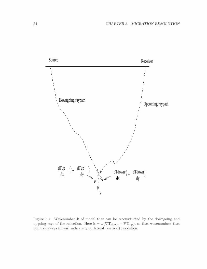
The above formulas are restricted to homogeneous velocity media, but the real earth isinhomogeneous in velocity. Resolution estimates can be obtained for inhomogeneous mediaby using the simple idea that the sum of the unit vectors of the downgoing and negativeupgoing rays is proportional to the wavenumber kmodel of the model that can be recon-structed For example, the ZO vertical rays suggest that the wavenumber of the model thatcan be reconstructed is proportional to #kmocel = (0, 0, 2π/λ). Note, the kx and ky com-ponents are zero because the ray is perfectly vertical and has no x-y component (Gesbert,2003). Formally, the model wavenumber that can be reconstructed (see Figure 3.7) is givenby

#k = ω∇(τdown(x) + τup(x)). (3.9)

Similar considerations can be used to estimate resolution for tomographic images (Shengand Schuster, 2003).


0 1 2 3 4 5 6 7 8 9 10 11−200

−180

−160

−140

−120

−100

−80

−60

−40

−20

0

Depth (m)

Midpoint (m)

∆ z / λ = 1

Depth Resolution Test: Interference of reflections for Different Layer Thickness/Wavelength Ratios

∆ z / λ = 0.8 ∆ z / λ = 0.6 ∆ z / λ = 0.4 ∆ z / λ = 0.2

Figure 3.4: Vertical resolution limit is reached when the thickness between two neighboringreflectors ∆z = λ/4.


TABA

TACA

TABA

TACA

A

B

C

dz

B C

A

1st Fresnel Zone BC=dx

−TACA TABA

−TACA TABA

T

= T/2

= T/2

dz = /4λ

λdx z /2

Figure 3.5: Extent of horizontal (left) and vertical (right) Fresnel zones for a ZO trace,where the 1st Fresnel zone defines the area where the difference in the shortest and longestraypath is equal to half the wavelength. The approximation formula for horizontal resolutionis valid when AB is much larger than λ.


Is it really important to be concerned about the subtle nuances of improving lateralresolution? Jianhua Yu shows in Figure 3.8 that modest lateral resolution leaves doubtabout the existence of fault, but slightly improving this lateral resolution via migrationdeconvolution leaves no doubt about the existence of a fault.

Beylkin Resolution → Migration Stretch. A simple interpretation of equation 3.9 isthat it is equivalent to the formula for migration stretch. Specifically, the migration stretchformulas in the different coordinate directions are given by differentiating the traveltimeformula 3.8 with respect to the coordinates of the trial image point (x, y, z):

∂τ/∂x = ∂τsx/∂x+ ∂τxg/∂x,

∂τ/∂y = ∂τsx/∂y + ∂τxg/∂y,

∂τ/∂z = ∂τsx/∂z + ∂τxg/∂z.

(3.10)

Using a Fresnel-zone argument, we set ∂τ ≈ T/2 and ∂x ≈ ∆x, ∂y ≈ ∆y and ∂z ≈ ∆z onthe left hand side of the above equation, and rearrange terms to get analytical expressionsfor the resolution limits (∆x,∆y,∆z), or migration stretch in the three coordinates similarto the expression in Figure 3.6. Here, T is the dominant period of the wavelet. Multiplyingthe three stretch formula in equation 3.10 by ω yields the components proportional to theBeylkin wavenumber formula in equation 3.9 (e.g., recall ω∂τ/∂x = kx). This establishesthe equivalency between Beylkin’s fancy resolution formula and the well known migrationstretch formulas.

3.3 Summary

Both time migration and spatial resolution are defined. The Beylkin stretch formula is usedso that the user decides the acceptable horizontal resolution at a selected depth region anduses the stretch formulas to estimate aperture width. The best vertical resolution you canachieve is λmin/4 but the best horizontal resolution is estimated by a complicated stretchformula that is a function of source and receiver coordinates.

Unlike depth migration, time migration does not suffer from migration stretch but doessuffer from mispositioning of events in complex geologic areas. Therefore it is rarely usedtoday for subsalt imaging. However, the velocity model must be finely tuned in order to getdepth imaging to show a coherent section. This compares to time migration which usuallyprovides a good looking image because the stacking velocity is used to estimate the time-migration velocity. The stacking velocity is robustly estimated by efficient and automaticvelocity scans while the velocity model for depth migration is typically estimated by atime-consumming and tedious process (e.g., reflection tomography or migration velocityanalysis).

3.4 Exercises

1. The CDP interval in Figure 7 is 50 m. The velocity at z = 1 km is 2 km/s andat z = 2.5 km it is 4 km/s, and the recording aperture is 350 CDP’s wide for any

3.4. EXERCISES 53

TABA

TACA

1st Fresnel Zone

A

B C

BC=dx

’

’

A’

dx λ z4L

L

−TACA TABA’ ’ = T/2

Figure 3.6: Extent of horizontal Fresnel zone for a trace with non-zero offset between thesource and receiver. The 1st horizontal Fresnel zone for a reflection defines the area wherethe difference in the shortest and longest reflection raypaths is equal to half the wavelength.


dTdown dTdowndx dy

i + j

Source Receiver

k

dx dyi + jdTup dTup

Upcoming raypathDowngoing raypath

Figure 3.7: Wavenumber k of model that can be reconstructed by the downgoing andupgoing rays of the reflection. Here k = ω(∇Tdown + ∇Tup), so that wavenumbers thatpoint sideways (down) indicate good lateral (vertical) resolution.

3.4. EXERCISES 55

Figure 3.8: 3D prestack migration images (left) before and (right) after migration deconvo-lution. Lateral resolution improves by about 20 percent so that the right image leaves nodoubt about the existence of a fault.


shot point. Calculate the minimum horizontal and vertical resolutions for a prestackmigration image at the points (x, z) = (0 km, 1 km), (x, z) = (1 km, 1 km), (x, z) =(0 km, 2.5 km), and (x, z) = (1 km, 2.5 km). Same question as before, except calculateminimum horizontal and vertical resolutions for a poststack migration image. Showwork.

2. Using fat circles and fat ellipses, compare the vertical and horizontal resolution limitsfor poststack migration and prestack migration for a point at (x, z) = (1 km, 2.5 km)in Figure 7. Assume a homogeneous velocity.

3. Convert your poststack depth migration code into a prestack time migration code.The output should be in the offset-time domain. Show poststack depth and timemigration images.

4. Determine the maximum aperture for a seismic experiment in order to image 0− 40degree dips at z = 5 km. Assume a homogeneous velocity of 5 km/s. What isthe minimum geophone spacing in order to not spatially alias the data? Assume aminimum wavelet period of 0.01 s. Clearly show steps in your reasoning.

5. Derive and use the Beylkin stretch formulas (starting point for derivation is equa-tion 3.10) to estimate the best horizontal and vertical resolutions for a 12 km widepoststack depth section at the following coordinates: (0,12), (12,12), (6,12), (6,6),(0,6), (3,3), (0,12). Assume the origin of coordinate system is at upper left portionof migration section and positive z is pointing downward. Assume a homogeneousvelocity of v = 3 km/s from 0-3 km, v = 5 km/s from 3-7 km, and any deeper than7 km we have a velocity of 6 km/s. Assume a maximum useful frequency of 80 Hz.Assume straight rays everywhere. Why is there better horizontal resolution at shallowdepths?

6. Time migrate the radar data from your lab exercise. Choose a suitable time migrationvelocity by trial and error. Show results. Which results look more coherent, thetime migration or depth migration results? Why does depth migration suffer frommigration stretch which is avoided by time migration. Wgat are benefits and liabilitiesof time migration vs depth migration?

7. Estimate the horizontal wavelength of surface waves and body wave reflections in theSaudi shot gather (from a previous lab). What is a good array interval that wouldsuppress surface waves but retain body waves ion the data. Test your estimate byapplying an N-point spatial averaging filter to the data, where N is length of yourestimated filter. Show results.

3.4. EXERCISES 57

*

migration resolution - king abdullah university of science ... · pdf file52 chapter 3....

Documents