Migration Correlation: Definition andEfficient Estimation

P. Gagliardini∗, C. Gouriéroux†

First version: November 2003This version: April 2004

∗Università della Svizzera Italiana, and CREST. Corresponding author: PatrickGagliardini, Institute of Finance, Università della Svizzera Italiana, Via Buffi 13, 6900Lugano, Switzerland. E-mail: gagliarp@lu.unisi.ch. Tel: +41 91 912 4723. Fax: +41 91912 4647.

†CREST, and University of Toronto.

We acknowledge G. Barone Adesi and two anonymous referees for very helpful comments.

1

Migration Correlation: Definition and Efficient Estimation

Abstract

The aim of this paper is to explain why cross-sectional estimated migra-tion correlations displayed in the academic and professional literature canbe either not consistent, or inefficient, and to discuss alternative approaches.The analysis relies on a model with stochastic migration in which the pa-rameters of interest, that are migration correlations, are precisely defined.The impossibility of estimating consistently the migration correlations fromcross-sectional data only is emphasized. We explain how to handle withindividual rating histories, how to weight appropriately the cross-sectionalestimators and how to estimate efficiently the joint migration probabilitiesat longer horizons.

Keywords: Credit Risk, Migration, Migration Correlation, Stochastic Tran-sition, Rating.

JEL Number: C23, C35, G11

2

1 Introduction

The risk on a portfolio of corporate credits (including corporate bonds) de-pends on the level of individual default and recovery rates of the differentborrowers, but also on their possible dependence. This dependence can bethe consequence of structural links between the firms. For instance the fail-ure of a firm can increase the default rate of its suppliers, which can implychains of failures. This dependence can also be due to more general factors,which affect the general state of the economy, and the situation of all firms,or of a group of firms. For instance an increase of the exchange rate of theEuro versus $ can diminish (resp. increase) the default rate of exporting(resp. importing) US firms.Typically the total risk in a portfolio of credits (with positive allocations)

is higher when the risks are positively correlated than when they can be as-sumed independent. Moreover this correlation effect cannot be suppressedby diversification. Even for portfolios including a large number of creditsof similar types and sizes, the effect of the underlying common risk factorscannot be eliminated. Therefore the analysis of default correlation is a nec-essary step for understanding credit portfolio diversification and determiningthe capital required to compensate credit risk [see e.g. Gordy (1998), Nag-pal, Bahar (1999), (2000), (2001)a, b, Lucas et alii (2001)]. In particularthe importance of default correlation (and of migration correlation) has beenrecognized by the regulator and its value is a significant input in the com-putation of the required capital by means of the quantile of the portfoliocredit losses (CreditVaR) [see The Basle Committee on Banking Supervision(2002)]. Since the CreditVaR is very sensitive to the value of the default cor-relation, this parameter has to be estimated carefully. An underestimationof the default correlation will imply an underestimation of the risk and a toolow level of required capital. An unbiased, but inaccurate estimation of thedefault correlation will induce levels of required capital which are too erraticwith respect to time.Default correlations are generally deduced from data basis on default his-

tories1. These basis correspond to panel data doubly indexed by individual(firm) and time. A special econometric literature is devoted to panel data.Indeed the total number of observations depend on the number of individuals(firms) in the panel [cross-sectional dimension] and of the number of obser-

1or rating histories for migration correlations.

3

vation dates [time dimension]. Thus a large number of observations can beobtained with a large cross-sectional dimension, a large time dimension, orboth. The need for large cross-sectional or time dimension will depend on theparameters of interest. Loosely speaking a large cross-sectional dimension al-lows for accurate estimation of parameters with "individual" interpretation,but a large time dimension is also needed for the estimation of parameterswith dynamic interpretations.The aim of this paper is to discuss in the panel framework the standard

descriptive estimation methods proposed in the literature to approximatedefault correlation or migration correlation [see e.g. Lucas (1995), Nagpal,Bahar (2001)b] and largely applied by practitioners and rating agencies forthe computation of CreditVaR2 [see e.g. de Servigny, Renault (2002)]. Thesemethods are generally introduced without specifying a model driving transi-tions and, as we will see, they can be neither consistent, nor efficient. Ourspecific contribution is to provide a framework where a precise definitionof migration correlation can be given and the consistency and efficiency ofthe estimators can be discussed. In addition, a more accurate estimator ofmigration correlations at longer horizons is presented.The rest of the paper is organized as follows. In Section 2 the cross-

sectional estimation method is reviewed and discussed. In particular its lackof consistency is pointed out. A precise definition of migration correlation isgiven in Section 3, by considering a model with stochastic transition matrix.The inconsistency of the cross-sectional estimator in this framework is dis-cussed in Section 4. Then a consistent estimator of the migration correlationat horizon 1 is introduced in Section 5. In Section 6 it is explained howto deduce the migration correlations at longer horizons from the migrationcorrelations at horizon 1. The finite sample properties of the different esti-mators are compared in a Monte-Carlo study presented in Section 7. Finally,Section 8 concludes.

2Other estimation approaches of default correlations are also considered in Finance.Some are based on the observation of equity prices, such as in the KMV approach, or onthe observation of bond prices [Lando (1998), Duffie, Singleton (1999), Gourieroux, Mon-fort, Polimenis (2003)]. In particular they are used for pricing various credit derivativesproposed in the market. They can only be applied to large firms, quoted on the market,issuing bonds regularly. However for the regulator the CreditVaR has to be computed forthe whole credit portfolio, including small or medium size firms, with a lot of over-the-counter credits. In this case the estimation approach from individual rating histories isthe only possible one. The same remark applies for portfolios of retail credits includingtheir derivatives, like the mortgage backed securities.

4

2 Calculating one year migration correlation[from Lucas (1995)]

In the financial literature the estimation of migration correlation has beenintroduced directly without defining precisely the parameter of interest and”without relying on a specific model driving transitions” [de Servigny, Re-nault (2002)] 3. This section follows the usual presentation [see e.g. Lucas(1995), Nagpal, Bahar (2001)b]. The available data consists in a panel ofrating histories:

Yi,t, i = 1, ..., n, t = 1, ..., T,

where i denotes the individual (either the firm, or the bond) and t the year.The variable Yi,t is polytomous qualitative, with alternatives k = 1, ..., K,indicating the different admissible grades. In general one of these alterna-tives corresponds to default, k = K say. For instance there are eight gradesfor Standard & Poor’s from the highest rating AAA to debt in default pay-ment D, when the ratings C, CC, CCC are aggregated. The cross-sectionaldimension is from n = 10000 for Moody’s, S&P’s where the data concernlarge international firms, up to n = 130000 for the French Central Bank,which follows all French firms including small and medium size firms. Thetime unit is generally the year, leading to a time dimension of T = 15− 20.Thus the cross-sectional dimension is much larger than the time dimension[see Foulcher, Gouriéroux, Tiomo (2003) for a comparison of the ratings ofthe main rating agencies Moody’s, S & P’s, Fitch and of the French CentralBank].At any given year t, we can compute the structure of individuals (firms or

bonds) per rating grade: (Nk,t, k = 1, ...,K), where Nk,t denotes the numberof firms (bonds) in grade k at t. We can also consider the transitions. IfNkl,t, k, l = 1, ..., K, denote the number of firms (bonds) migrating fromrating class k at t− 1 to rating class l at date t, the transition probabilitiesare approximated by: bπkl,t = Nkl,t

Nk,t−1, (say).

Such matrices are regularly reported by Moody’s, S & P, the French CentralBank, etc [see e.g. Brady, Bos (2002), Brady, Vazza, Bos (2003), Bardos,

3This can explain the following remark by Lucas (1995) p82: "These historical statisticsdescribe only observed phenomena, not the true underlying correlation relationship".

5

Foulcher, Bataille (2004)]. They summarize the individual migrations of agiven firm. Such an estimated transition matrix is given in Table 1.It is usually considered that joint migrations can be analyzed in a similar

way, by calculating the ratio between the number of pairs of firms (bonds) ina given rating class, which actually migrated to a given category (for exampledefault), and the total number of pairs of firms (bonds) in the rating class.Then an estimator is defined by:

bpkl,t = Nkl,t (Nkl,t − 1)Nk,t−1 (Nk,t−1 − 1) , (1)

where k [resp. l] is the starting grade [resp. the final grade]. The intuitiveidea is to approximate a ”probability of joint migration” by drawing the pairsof bonds without replacement in the population and taking the empiricalcounterpart. This type of estimator is standard in survey sampling theory,where it is used to estimate the so-called second order inclusion probabilityinvolved in the Horvitz-Thompson estimator [see e.g. Kish (1967), Konijn(1973)]. However it is clearly inappropriate in the framework of defaultcorrelation. Let us study what the quantity bpkl,t is really approximating. Itis immediately realized that, for a large portfolio (n ∼ ∞), both Nk,t−1 andNkl,t will be large and: bpkl,t ∼ bπ2kl,t.Thus, in our framework of large cross-sectional dimension, the estimatorsbpkl,t, k, l = 1, ...,K, bring no additional information than the estimatorsbπkl,t, k, l = 1, ...,K, of the individual transitions and in particular cannotbe used to measure a notion of joint migration. A similar argument can begiven for the migration correlations. The cross-sectional estimator is givenby: bρkl,t = bpkl,t − (bπkl,t)2bπkl,t (1− bπkl,t) . (2)

If the size n of the portfolio is large, estimator bpkl,t is close to (bπkl,t)2, andbρkl,t is close to zero, no matter of the true value of the underlying migrationcorrelation4.This argument5 will be developed in greater details in the next section,4Estimator bρkl,t is numerically equal to −1/(Nk,t−1 − 1).5The same argument holds for the modified estimator of de Servigny, Renault (2002)

corresponding to drawing with replacement, introduced to avoid negative estimated prob-abilities of joint migration.

6

where a model with stochastic transition is introduced and used to definethe parameters of interest, that are the probabilities of joint migration or themigration correlations.

3 Stochastic migration intensity

A basic model for understanding migration dependence is the extension ofthe stochastic intensity model introduced for default risk [see e.g. Lando(1998), Duffie, Singleton (1999), Gouriéroux, Monfort, Polimenis (2003)].This specification assumes that the rating chains (Yi,t, t varying) , i = 1, ..., n,are independent identically distributed Markov processes, when the commontransition matrices (Πt), with elements πkl,t, are given, and the model iscompleted by assuming that the transition matrices are stochastic. For ex-pository purpose, we assume6:

Assumption A.1: The transition matrices at horizon 1 are stochastic, in-dependent with identical distributions (i.i.d.).

Thus the joint (serial and instantaneous) dependence between ratings passesthrough the stochastic transition. This explains why it is not possible toidentify "whether historical fluctuations in default rates are caused by de-fault correlation or simply by (stochastic) changes in default probabilities"[Lucas (1995), p82]. We get a nonlinear factor model in which the factors arethe elements of the transition matrices. The number of independent factorsis (K − 1)2 due to the unit mass restrictions on transition probabilities andthe interpretation of default as an absorbing barrier.Since the underlying time dependent transition matrices are not observ-

able, the joint distribution of rating chains has to be derived by integratingout the unobservable factor Πt. When the transitions have been integratedout, the joint rating vector (Y1,t, ..., Yn,t)

0still defines an homogeneous Markov

chain [see Appendix 1] with Kn admissible states. In practice K = 10, thenumber of firms is several thousands (about 10000 for the data base of S &P, 130000 for the data base of the French Central Bank) and the state space

6See Gagliardini, Gouriéroux (2003) for the general framework of serially dependentstochastic transition matrices. For serially dependent transition matrices, the migrationcorrelation has to be defined conditional on the whole rating histories, not only the lastrating; but consistent estimators of the path dependent migration correlation can also bederived, and differ from the estimator introduced in this paper.

7

dimension of the joint rating chain is for instance 1010000 7. Therefore thetransitions corresponding to the joint rating processes are difficult to display,even in the framework of Assumption A.1. However this framework is ap-propriate for a first analysis of joint migration of a pair of firms (or bonds).For instance there is dependence between the ratings of two different firms(bonds), given their lagged ratings. The migration dependence is a conse-quence of the unobservable factor which jointly influences the ratings of allfirms (bonds). Typically the realization at date t of the transition matrixΠt can correspond to a matrix with larger probabilities of downgrades (resp.upgrades), which will imply more (joint) downgrades (resp. upgrades) of in-dividual ratings. This effect is illustrated below in Figure 1, where two ratinghistories are displayed8.

[Figure 1: Simulated rating histories]

Due to a regime switching of the transition matrix, we observe some un-derlying effect towards downgrades at dates 7 and 13. This implies jointdowngrades, but with different sensitivities for the two firms.In the stochastic transition framework it is now possible to define precisely

the parameters of interest. For this purpose let us focus on a pair of firms(bonds) i, j 9. The bivariate process (Yi,t, Yj,t) is also an homogeneous Markovprocess [see Appendix 1] with state space including the admissible pairs ofgrades (k, l). Let us consider its transition matrix. The elements of thismatrix are joint transition probabilities defined by:

pkk∗,ll∗ = P [Yi,t+1 = k∗, Yj,t+1 = l∗ | Yi,t = k, Yj,t = l] . (3)

These joint transition probabilities do not depend on the selected couple offirms (bonds) (i, j). Moreover they admit a simple expression in terms of thestochastic transition probabilities10:

pkk∗,ll∗ = E [πkk∗,tπll∗,t] . (4)

7The number of firms is still large if the homogeneity (i.i.d.) assumption is introducedon subsets of firms to account for region or industry specific effects [see e.g. Nagpal, Bahar(2001)].

8The simulation is based on the three states ordered probit model presented in Section7.

9It would be also possible to consider joint migration for three, four, etc, firms inorder to study migration clustering phenomenon [see Gouriéroux, Monfort (2002) for theanalysis of clustering for default risk].10The expressions of the joint transition probabilities are modified when the stochastic

8

Instead of the joint migration transition matrix, it is also possible to definethe migration correlation11:

ρkk∗,ll∗ = Corr£IYi,t+1=k∗, IYj,t+1=l∗ | Yi,t = k, Yj,t = l

¤, (5)

where IY=k = 1, if Y = k, and 0 otherwise. The migration correlation isequal to:

ρkk∗,ll∗ =pkk∗,ll∗ − αkk∗αll∗p

αkk∗ (1− αkk∗)pαll∗ (1− αll∗)

, (6)

where: αkk∗ = E [πkk∗,t] is the expected transition probability. The migrationcorrelation can be written as:

ρkk∗,ll∗ =cov (πkk∗,t, πll∗,t)p

αkk∗ (1− αkk∗)pαll∗ (1− αll∗)

= corr (πkk∗,t, πll∗,t)

sV (πkk∗,t)

αkk∗ (1− αkk∗)

sV (πll∗,t)

αll∗ (1− αll∗),

where V (π) denotes the variance of π. In the latter decomposition, thefirst component corr (πkk∗,t, πll∗,t) measures the link between the underlyingtransition probabilities. The two other terms account for the relationshipbetween the discrete rating indicators IY=k and the continuous transitionprobabilities.To summarize, joint (bivariate) migrations can be equivalently described

in terms of the (K2,K2) matrices p or ρ. All joint migrations provide infor-mation on the risk of a credit portfolio, and have to be estimated. Howeverfor illustration some specific ones are often presented and discussed. For in-stance the joint migration towards default corresponds to k∗ = l∗ = K, andis summarized by K2 different numbers. The up-up migrations correspondsto k∗ = k + 1, l∗ = l + 1, that is to joint upgrade by one tick. There exist(K − 1)2 such measures. Similarly it is possible to define down-down, andup-down migration probabilities. At this step it is important to note that the

transition matrices are serially correlated. Indeed the expectation has to be evaluatedconditional on the whole individual rating histories. Since the parameter of interest has adifferent expression, its consistent estimator has to be modified accordingly [see Gagliar-dini, Gouriéroux (2003)].11The joint transition probabilities pkk∗,ll∗ are often called migration correlations in the

literature. It seems important to distinguish the definitions of p and ρ to avoid misleadinginterpretations.

9

Basle Committee has recently proposed to account for migration correlation,but has only proposed a model when k∗ = l∗, k = l, which is not sufficientto take account of all dependences [see The Basle Committee on BankingSupervision (2002)].At the end of Section 3 and under Assumption A.1, the parameters of

interest either the joint migration probabilities pkk∗,ll∗, or the associated mi-gration correlations ρkk∗,ll∗ are clearly defined.

4 Non-consistency of the cross-sectional esti-mator

Let us explain the reason for the inconsistency of the cross-sectional estima-tor, when the cross-sectional dimension n is large. As mentioned in Section 2,for large portfolios (n ∼ ∞), the cross-sectional estimator bpkl,t converges toπ2kl,t and not to the parameter of interest pkl,kl corresponding to the diagonalterm defined in equation (3). This result is a consequence of the factor rep-resentation of the rating processes. Conditional on Πt,Πt−1, ... the individualrating chains are independent identically distributed. Thus the strong law oflarge numbers can be applied conditional on the factors and we get:

limn→∞

bpkl,t = π2kl,t. (7)

The possibility of applying the law of large numbers and the central limittheorem conditional on the factors corresponds to the so-called infinitely finegrained assumption proposed by the Basle Committee. In particular, if thenumber of firms (bonds) n is large, the realization of the transition matrix atdate t will be completely known. In fact it is easily seen that the set of empir-ical transitions (bπkl,t, k, l = 1, ...,K, t = 1, ..., T ) is a sufficient statistics forthe model with stochastic transition. From the cross-sectional informationat year t, it is at best possible to reconstitute the transition matrix Πt. Butit is not possible to reconstitute the matrices p and ρ. In financial termsthe systematic risk Πt cannot be eliminated by a cross-sectional averaging,that is by individual diversification. For instance an unbiased estimation ofa covariance Cov (πkk∗,t, πll∗,t) requires at least two dated observations of thetransition, that is three successive years of data, and a pure cross-sectionalapproach cannot allow for identifying joint migrations.

10

At a first sight it can be surprising that the cross-obligor default corre-lation cannot be estimated consistently from an infinite number n of (cross-sectional) data. In fact it is important to note that different asymptotictheories can be considered in a panel framework according to the dimension,either n, or T , which tends to infinity. Some parameters, such as the transi-tion matrix of date t, can be estimated consistently when n tends to infinityand only one observation date (that is t) is available. Other parameters, suchas the migration correlations, have an interpretation involving time and needalso T tending to infinity to be consistent12.The same argument applies to the maximum likelihood estimator consid-

ered by Gordy, Heitfield (2002) in a model where Πt = Π is time independentand stochastic. The time dimension is not sufficient to get consistency sincethe data are both with equal correlation with respect to time and individual.

5 A time averaged estimator

Let us assume a rather large portfolio (n/K ≥ 30 approximately) and severalyears of observations. In a first step the underlying transition probabilities(πkl,t) will be replaced by their cross-sectional empirical counterparts (bπkl,t).Then the parameter of interest p or ρ will be approximated by averagingon time. More precisely, from equation (4), the joint migration probabilitypkk∗,ll∗ is the common mean of all the products πkk∗,tπll∗,t, t = 1, ..., T. Fora large portfolio, we have [by central limit theorem applied conditional on(Πt)]: bπkk∗,tbπll∗,t ' πkk∗,tπll∗,t + ukk∗,ll∗,t, t = 2, ..., T, (8)

where V (ukk∗,ll∗,t) = ωkk∗,ll∗, say, is independent of the year. We deducethat: bπkk∗,tbπll∗,t ' pkk∗,ll∗ + ukk∗,ll∗,t + vkk∗,ll∗,t, t = 2, ..., T, (9)

where vkk∗,ll∗,t = πkk∗,tπll∗,t − pkk∗,ll∗ are i.i.d. errors with zero-mean and avariance independent of t (Assumption A.1). Moreover the errors u and vare independent. The relation (9) defines a linear model, with the constant

12Generally the consistency of an estimator requires some geometric ergodicity condi-tion on the observations, that is a correlation between observations tending to zero at ageometric decay rate with the distance between the observation indexes: ∃r, 0 ≤ r < 1,c > 0 such that |corr (Yi,t, Yj,t) | Yi,t−1 = k, Yj,t−1 = l| ≤ crj−i. This condition is typicallynot satisfied in the present framework where the cross-sectional correlation is constant.

11

as explanatory variable, pkk∗,ll∗ as the parameter. Since the model is ho-moscedastic, the optimal weights to compute the least squares estimator areidentical. Thus the estimator is:

bpkk∗,ll∗ = 1

T − 1TXt=2

bπkk∗,tbπll∗,t. (10)

The estimator of the migration correlation is [see equation (6)]:

bρkk∗,ll∗ = bpkk∗,ll∗ − bαkk∗bαll∗pbαkk∗ (1− bαkk∗)pbαll∗ (1− bαll∗)

, (11)

where bαkk∗ =1

T−1PT

t=2 bπkk∗,t. The estimators of matrices p or ρ are consis-tent when both the cross sectional and time dimensions, n and T , respec-tively, tend to infinity. When n is large bπkk∗,tbπll∗,t is close to πkk∗,tπll∗,t andthe approximated linear model (9) is valid. For n large, the OLS estimatoris unbiased, efficient (among linear estimators). However its variance can befar from zero if T is small. Thus the additional condition T →∞ is neededto get the consistency of the OLS with T aggregated transitions.The consistency result is valid if the Markov chain is recurrent ergodic.

It is important to note that the recurrence condition, that is the fact thatthe chain visits each state an infinite number of dates, is not satisfied whenthe state space includes an absorbing barrier, such as default. However therecurrence condition can be recovered if the population of interest is renewedat each date. More precisely it has to be assumed that some new firmsare created to balance the defaulted individuals. This latter assumption isapproximately satisfied for the data base of the rating agencies and of theFrench Central Bank [see Gagliardini, Gouriéroux (2003) for a more detaileddiscussion].Estimators of the joint (bivariate) transition probability averaged on sev-

eral dates have already been considered in the literature [see e.g. Bahar,Nagpal (2001)b, de Servigny, Renault (2002)], without underlying statisti-cal model and without any justification in terms of consistency or efficiency.They have often been defined with different weights for the different dates.For instance the estimator of pkl,kl introduced by Bahar, Nagpal (2001)band by de Servigny, Renault (2002) are considered below. The estimator byBahar, Nagpal (2001)b is:

epkl,kl = PTt=2Nkl,t (Nkl,t − 1)PT

t=2Nk,t−1 (Nk,t−1 − 1)∼PT

t=2N2kl,tPT

t=2N2k,t−1

=TXt=2

N2k,t−1PT

t=2N2k,t−1

bπ2kl,t.12

It is easily checked that, if n is large, and if the population is renewed toensure the recurrence of the chain, we get:

N2k,t−1 ∼ n2p2k,

TXt=2

N2k,t−1 ∼ (T − 1)n2p2k,

where (pk) is the marginal distribution of the chain, and therefore epkl,kl ∼bpkl,kl. Thus the introduction of weights is absolutely not necessary. Similarlythe estimator proposed by de Servigny, Renault (2002) is given by:

TXt=2

Nk,t−1PTt=2Nk,t−1

bπ2kl,t,and the same remark applies.

6 Longer horizons

It is a common practice to use the estimation formula (10) simultaneouslyfor different horizons [see e.g. Nagpal, Bahar (2001)]. For instance the jointbivariate transition probability at horizon 2:

pkk∗,ll∗(2) = P [Yi,t+2 = k∗, Yj,t+2 = l∗ | Yi,t = k, Yi,t = l] , (12)

is estimated by:

epkk∗,ll∗(2) = 1

T − 2TXt=3

bπkk∗,t(2)bπll∗,t(2), (13)

where bπkk∗,t(2) denotes the empirical cross-sectional transition probabilityfor period (t− 2, t) . It is important to note that it is not appropriate to usesimultaneously the empirical estimator of the joint transition probability fordifferent horizons. Indeed, whereas bpkk∗,ll∗ is efficient for pkk∗,ll∗, the es-timator epkk∗,ll∗(2) can be improved, by taking into account the informationincluded in the statistical model. Indeed, under Assumption A.1, the tran-sition matrices at horizon 2 such as Πt(2) = Πt−1Πt and Πt+1(2) = ΠtΠt+1

depend on the common matrix Πt and therefore are dependent. Thus As-sumption A.1 cannot be satisfied simultaneously at horizons 1 and 2. UnderAssumption A.1 the estimators bΠt(2) and bΠt+1(2) are also dependent, since

13

they are computed on overlapping periods. Loosely speaking the estimatorep computed from T = 20 observations for horizon 7 [see e.g. Nagpal, Bahar(2001)] has an accuracy equivalent to an estimator under independence com-puted from about 20/7 ∼ 3 observations. Therefore it is not very accuratedue to the non-consistency of cross-sectional estimators 13.A better accuracy can be recovered along the following lines. By the law

of iterated expectations the joint transition probability at horizon 2 can bewritten as:

pkk∗,ll∗(2) = E [πkk∗,t(2)πll∗,t(2)]

=Xm

Xn

E [πkm,t−1πmk∗,tπln,t−1πnl∗,t]

=Xm

Xn

E [πkm,t−1πln,t−1]E [πmk∗,tπnl∗,t]

=Xm

Xn

pkm,lnpmk∗,nl∗ .

An estimator with an accuracy of the same order of magnitude as bpkk∗,ll∗, thatis taking into account the whole time dimension, and which is asymptoticallyefficient is: bpkk∗,ll∗(2) =X

m

Xn

bpkm,lnbpmk∗,nl∗, (14)

where bpkm,ln is given by formula (10) applied to horizon 1. This approachis easily understood if it is noted that under Assumption A.1 the bivariateprocess (Yi,t, Yj,t) is a Markov process of order 1 with transition matrix:

P = [pkk∗,ll∗] .

Therefore its transition matrix at horizon 2 is:

P (2) = P 2,

which is precisely the formula used in (14).Estimators for any horizon h corresponding to (13) and (14) are derived

in a similar way by formula P (h) = P h.

13The same remark applies to the ten-year default correlations estimated in Lucas(1995).

14

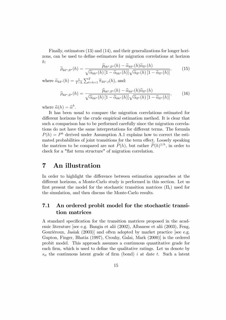
Finally, estimators (13) and (14), and their generalizations for longer hori-zons, can be used to define estimators for migration correlations at horizonh: eρkk∗,ll∗(h) = epkk∗,ll∗(h)− eαkk∗(h)eαll∗(h)peαkk∗(h) [1− eαkk∗(h)]

peαll∗(h) [1− eαll∗(h)], (15)

where eαkk∗(h) =1

T−hPT

t=h+1 bπkk∗,t(h), and:bρkk∗,ll∗(h) = bpkk∗,ll∗(h)− bαkk∗(h)bαll∗(h)pbαkk∗(h) [1− bαkk∗(h)]

pbαll∗(h) [1− bαll∗(h)], (16)

where bα(h) = bαh.It has been usual to compare the migration correlations estimated for

different horizons by the crude empirical estimation method. It is clear thatsuch a comparison has to be performed carefully since the migration correla-tions do not have the same interpretations for different terms. The formulaP (h) = P h derived under Assumption A.1 explains how to correct the esti-mated probabilities of joint transitions for the term effect. Loosely speakingthe matrices to be compared are not eP (h), but rather eP (h)1/h, in order tocheck for a "flat term structure" of migration correlation.

7 An illustration

In order to highlight the difference between estimation approaches at thedifferent horizons, a Monte-Carlo study is performed in this section. Let usfirst present the model for the stochastic transition matrices (Πt) used forthe simulation, and then discuss the Monte-Carlo results.

7.1 An ordered probit model for the stochastic transi-tion matrices

A standard specification for the transition matrices proposed in the acad-emic literature [see e.g. Bangia et alii (2002), Albanese et alii (2003), Feng,Gouriéroux, Jasiak (2003)] and often adopted by market practice [see e.g.Gupton, Finger, Bhatia (1997), Crouhy, Galai, Mark (2000)] is the orderedprobit model. This approach assumes a continuous quantitative grade foreach firm, which is used to define the qualitative ratings. Let us denote bysit the continuous latent grade of firm (bond) i at date t. Such a latent

15

grade is sometimes computed regularly by the rating specialists, especiallyfor internal ratings. Generally it is confidential and has to be consideredas unobservable. In other approaches based on Merton’s model [see Merton(1974)], this latent grade is defined as the ratio of asset value and liabili-ties14. It is also unobservable, whenever a detailed balance sheet of the firmis unknown. The ordered probit model [see e.g. Maddala (1986), Gouriéroux(2000)] is defined by i) specifying the latent model, that is the dynamics ofthe latent variables, and ii) by explaining how the observable endogenousvariables, that are the qualitative ratings, are related to the underlying con-tinuous grades.

i) The latent model

Let us assume known the ratings of the different firms (bonds) at date t− 1.Given these ratings, we assume that the underlying grades sit, i = 1, ..., n,t = 1, ..., T, can be written as:

sit = αk + Zt + εit,

where the errors (εit) , i = 1, ..., n, and the common factor (Zt) are indepen-dent standard gaussian variables, and the intercept αk depends on the laggedrating Yi,t−1 = k of firm (bond) i. Note that the conditional distribution ofthe score of a firm given the past depends on the previous rating of the firmonly.

ii) The link between the latent and observed variables

Let us now consider a model with K = 3 states, where k = 3 denotes thedefault absorbing barrier. The qualitative ratings at date t are deduced bydiscretizing the underlying continuous grades:

Yit = l, iff cl−1 ≤ sit < cl,

where c0 = −∞ < c1 < c2 < c3 = ∞ are given thresholds. Then thetransition matrix is given by:

Πt =

Φ (a11 − Zt) Φ (a12 − Zt)− Φ (a11 − Zt) 1− Φ (a12 − Zt)Φ (a21 − Zt) Φ (a22 − Zt)− Φ (a21 − Zt) 1− Φ (a22 − Zt)

0 0 1

,

14In other words Merton’s model corresponds to a crude specification of the score, wherethe score coincides with this ratio. In the usual scoring methodology this ratio is oneexplanatory variable included among several other ones.

16

where the parameters akl = cl − ak, k, l = 1, 2, are set to15:

a11 = 1, a12 = 4, a21 = −1, a22 = 2 .Thus the first two rows of the transition matrix correspond to an orderedprobit model, with a common latent variable. This type of probit model hasbeen suggested for the analysis of credit risk. It has been proposed to identifythe common factor with one macroeconomic variable as a cycle indicator [seee.g. Bangia et alii (2003)] 16. This interpretation is difficult to test fromthe available data which concern a limited period of time. Moreover themodel has to be completed by a dynamic model for cycles. When the factoris let unspecified as in the present model, the transition matrix becomesstochastic by means of Zt. The distribution of the transition matrix Πt,that is the distribution of the four independent transition probabilities, hasa rather complicated form. However it is easy to derive its first and secondmoments by simulation. For this purpose the number of replications has beenfixed to 1000000. The expected transition matrix α = E (Πt) is given by:

α =

0.761 0.237 0.0020.240 0.682 0.0780 0 1

.

Thus, as observed in practice, the diagonal elements are rather large. More-over the values 0.237 and 0.240, corresponding to one tick downgrade andupgrade, are of the same order of magnitude. The class k = 1 is less riskythan k = 2 as revealed by the ranking of the associated default probabilities.Let us now consider the variance-covariance matrices of the first and secondrows, π1,t and π2,t, of Πt. They are are given by:

V (π1,t) =

0.056 −0.054 −0.002−0.054 0.053 0.001−0.002 0.001 0.001

, V (π2,t) =

0.055 −0.039 −0.016−0.039 0.040 −0.001−0.016 −0.001 0.017

,

whereas their covariance is:

Cov (π1,t, π2,t) =

0.042 −0.014 −0.028−0.041 0.014 0.027−0.001 −0.000 0.001

.

15The parameters satisfy the constraint: a11 + a22 = a12 + a21.16Under this interpretation, it would be necessary to assume serially dependent transi-

tion matrices to get dynamics of switching regimes.

17

Since the rows of the transition matrix sum up to 1, the rows and columnsof the variance and covariance matrices sum up to zero. Since the diagonalelements of the variance-covariance matrices have to be positive, at least onecorrelation is negative. Thus the unit mass restriction can be a source ofmisleading interpretations of the migration correlation sign.

7.2 Results

A Monte-Carlo study has been performed to analyze the finite sample prop-erties of the joint migration probability and migration correlation estimatorsdiscussed in Sections 2, 5 and 6. It is based on S = 10000 replications ofthe rating transitions of n = 1000 firms over T = 20 years in the orderedprobit model defined in Section 7.1. Note that the number of firms is keptfixed. The population is not renewed by introducing new created firms tobalance default. Even if the estimators are not consistent without renewingthe population, it is still possible to study the finite sample properties of theestimators.

7.2.1 Migration correlations at horizon 1

Table 2 displays the estimated joint (bivariate) transition probabilities athorizon 1 obtained by using the time averaged estimator. We focus on thecase k = l, k∗ = l∗, which corresponds to transitions with identical startingrating classes and identical final rating classes for the pair of firms. In Table3 we provide the corresponding results obtained using the cross-sectionalestimator evaluated at date t = 10. For both estimators we report theaverage, the median, the standard deviation, the Mean Squared Error (MSE),and the range between the α and 1− α quantiles, for α = 5% and 1%. Thetrue value of the corresponding parameters of interest are reported in Table4.For both estimators the expectation is very close to the true parame-

ter value, pointing out that they are both unbiased for the selected samplesizes. However, the two estimators strongly differ in terms of accuracy: thetime averaged estimator features better accuracy with respect to the purecross-sectional one. This is immediately seen by comparing the standarddeviations. For the estimator proposed in this paper, they are smaller by afactor of about

√20 ∼ 4.5. These findings are reinforced by comparing the

interquantile ranges, for α = 0.05, 0.01. These intervals are much tighter for

18

the time averaged estimator, indicating that its distribution is more concen-trated around the mean value. In order to better visualize these results, Fig-ures 2 and 3 display the histograms of the time averaged and cross-sectionalestimators, respectively, for the following transitions: (1, 1) → (2, 2) (jointdowngrade), (1, 1) → (3, 3) (joint default starting from the better rating),(2, 2) → (1, 1) (joint upgrade), and (2, 2) → (3, 3) (joint default startingfrom the worst rating).

[Insert Figure 2: Histogram of the distribution of the time averaged estimator]

[Insert Figure 3: Histogram of the distribution of the cross-sectional estimator]

The distributions corresponding to the cross-sectional estimator are muchmore dispersed and feature fatter tails. In particular, the distributions ofthe estimator admit a peak at 0, which implies a significant probability ofstrongly underestimating the joint migrations. The same type of feature willof course be observed with a time averaged estimator when the number ofobservation dates is too small.Similar tables can be derived for the time averaged and cross-sectional

estimators of the migration correlation matrix ρ. The estimates by the timeaveraged method (resp. the cross-sectional estimator) are provided in Table 5(resp. 6), whereas the true correlations are given in Table 7. It is immediatelyseen that the cross-sectional estimator of the ρ matrix is highly biased, withvalues uniformly close to zero.To summarize, the Monte-Carlo study shows that the theoretical inconsis-

tency of the cross-sectional estimator has serious consequences for any timeaveraged estimator with small finite time dimension T (even if the populationis not renewed), such as very erratic estimates and strong underestimationof the probability of joint migrations. This bias has direct consequences forrisk management. Indeed by underestimating the joint migrations we un-derestimate the default correlation and thus the risk included in the creditportfolio.

7.2.2 Longer horizons

Let us now consider the estimation of migration correlations at horizon longerthan 1. Table 8 displays the estimated bivariate transition probabilities athorizon h = 7 obtained using the standard estimator epkl,kl(7) defined inequation (13). The corresponding results for estimator bpkl,kl(7) taking into

19

account the Markov property [see equation (14)] are displayed in Table 9.The true value of the parameters of interest are reported in Table 10.Let us first consider the mean of the estimators. Both estimators fea-

ture a moderate finite sample bias, which is in general smaller for estimatorepkl,kl(7) 17. However, estimator bpkl,kl(7) is preferable in terms of the median.Indeed, for both estimators the median is often below the mean, but themedian of bpkl,kl(7) is generally closer to the true parameter value. In particu-lar, the median of epkl,kl(7) often underestimates quite severely the true jointmigration probability, especially in the cases of joint default. These featuresare confirmed by the empirical distributions of the two estimators, which arereported in Figures 4 and 5.

[Insert Figure 4: Histogram of the distribution of epkl,kl(7)][Insert Figure 5: Histogram of the distribution of bpkl,kl(7)]

The distributions of the elements of epkl,kl(7) are more skewed to the right,and assign a larger probability mass to values close to zero.Let us now consider the dispersion of the estimators. The distribution ofbpkl,kl(7) is more concentrated around the mean value, as deduced by compar-

ing the standard deviations and the interquantile ranges, or the histogramsof the estimators. It is important to note that the time averaged estimator,which is more precise than the cross-sectional one, is itself not very accurate.Finally, we can compare the results for migration correlations at horizon

h = 7 obtained using estimators eρkl,kl(h) and bρkl,kl(h) [see equations (15)and (16)], which are displayed in Tables 11 and 12, respectively. The truevalues of migration correlations are reported in Table 13. The empiricaldistributions of the estimators eρkl,kl(h) and bρkl,kl(h) are reported in Figures6 and 7, respectively.

[Insert Figure 6: Histogram of the distribution of eρkl,kl(h)][Insert Figure 7: Histogram of the distribution of bρkl,kl(h)]

The proposed estimator bρkl,kl(h) taking into account the Markov property isboth less biased and more accurate. In particular, migration correlations es-timated using the standard estimator eρkl,kl(h) are severely downward biased.Their use for computing a Credit VaR will automatically imply significantunderestimation of the required capital.17The (finite sample) bias of estimator bpkl,kl(7) is due to the fact that it is the power of

an unbiased estimator: bP (7) = bP 7.20

8 Concluding remarks

The aim of this paper was to define precisely the notion of migration cor-relation, in order to study the properties of the cross-sectional estimatorsand compare them with alternative estimators taking into account the timedimension and the dynamic properties of the underlying model. It has beenexplained why the cross-sectional estimator is not consistent and the Monte-Carlo study points out its poor performance even if the cross-sectional di-mension is large. In fact these basic cross-sectional estimators can be used todeduced the efficient time averaged estimator. We have also explained howto construct simultaneously the estimators of migration correlations at differ-ent horizons without loosing the information contained in the time dimensionand in the underlying model. Since the estimated migration correlations areimportant tools for evaluating the risk on a credit portfolio, the estimationbias or the lack of accuracy will induce errors in the corresponding requiredcapital. In practice by underestimating the true migration correlation, theestimated required capital will also be too small.Since mainly the time dimension matters (not the cross-sectional dimen-

sion), there is a need for rather long individual rating histories. In practicethe data bases of Moody’s, Standard & Poor’s, the French Central Bank, etcinclude between 15 and 20 years of reliable data. This is a minimal numberto estimate the one-year migration correlation under an i.i.d. assumption onthe underlying stochastic transition matrix. This is not sufficient to test thisassumption of flat term structure of migration correlation with a sufficientpower or to introduce more complicated dynamics on these transition matri-ces. This lack of time dimension is ever increased when some macroeconomiceffects on transitions are introduced, for instance when different distributionsof transition matrices are considered for recession and expansion periods [seee.g. Nickell, Perraudin, Varotto (2000), Bangia et alii (2002), and the dis-cussion in Klaassen, Lucas (2002)]. This approach is much more appropriatefor retail credits, such as classical consumption credit, mortgages, revolvingcredit, ... for which internal scores and ratings can be available on a monthlybasis, with a time dimension of T = 150− 200.

21

REFERENCES

Albanese, C., Campolieti, J., Chen, O., and A., Zavidonov (2003): "CreditBarrier Models", University of Toronto DP.

Bangia, A., Diebold, F., Krominus, A., Schlagen, C., and T., Schuermann(2002): ”Ratings Migration and Business Cycle, with Application to CreditPortfolio Stress Testing”, Journal of Banking and Finance, 26, 445-474.

Bardos, M., Foulcher, S., and E., Bataille (2004): "Les Scores de laBanque de France: Methode, Resultats, Applications", Observatoire des En-treprises, Banque de France.

Basle Committee on Banking Supervision (2002): "Quantitative ImpactStudy 3. Technical Guidance", Bank for International Settlements, Basel.

Brady, B., and R., Bos (2002): "Record Defaults in 2001. The Resultsof Poor Credit Quality and a Weak Economy", Special Report, Standard &Poor’s, February.

Brady, B., Vazza, D., and R., Bos (2003): "Ratings Performance 2002:Default, Transition, Recovery and Spreads", Website of Standard & Poor’s.

Carty, L. (1997): ”Moody’s Rating Migration and Credit Quality Corre-lation, 1920-1996”, Moody’s Investor Service.

Crouhy, M., Galai, D., and R. Mark (2000): ”A Comparative Analysis ofCurrent Credit Risk Models”, Journal of Banking and Finance, 29, 59-117.

Das, S., and G., Geng (2002): "Modelling the Processes of CorrelatedDefault", Working Paper, Santa Clara University.

Davis, M. (1999): "Contagion Modelling of Collateralized Bond Obliga-tions", Working Paper, Bank of Tokyo, Mitsubishi.

Davis, M., and V., Lo (2001): "Infectious Defaults", Quantitative Fi-nance, 1, 382-387.

De Servigny, A., and O., Renault (2002): ”Default Correlation: EmpiricalEvidence”, Standard and Poor’s, September.

22

Duffie, D., and K., Singleton (1999): "Modeling the Term Structure ofDefaultable Bonds", Review of Financial Studies, 12, 687-720.

Erturk, E. (2000): "Default Correlation Among Investment Grades Bor-rowers", Journal of Fixed Income, 9, 55-60.

Feng, D., Gouriéroux, C., and J. Jasiak (2003): "The Ordered Quali-tative Model for Rating Transitions", Discussion Paper, e-Finance Group,Montreal.

Foulcher, S., Gouriéroux, C., and A., Tiomo (2003): "La structure parterme des taux de défauts et de Ratings", Banque de France DP.

Frey, R., and A., McNeil (2001): "Modelling Dependent Defaults", Work-ing Paper, ETH Zurich.

Gagliardini, P., and C., Gouriéroux (2003): "Stochastic Migration Mod-els", CREST DP.

Gieseke, K., (2001): "Correlated Defaults with Incomplete Information",Working Paper, Humboldt University.

Gordy, M. (1998): "A Comparative Anatomy of Credit Risk Models",Journal of Banking and Finance, 24, 119-149.

Gordy, M., and E., Heitfield (2002): ”Estimating Default Correlationfrom Short Panels of Credit Rating Performance Data”, Working Paper,Federal Reserve Board.

Gouriéroux, C. (2000): Econometrics of Qualitative Dependent Variables,Cambridge University Press.

Gouriéroux, C., and A., Monfort (2002): "Equidependence in Qualitativeand Duration Models with Application to Credit Risk", CREST DP.

Gouriéroux, C., Monfort, A., and V., Polimenis (2003): ”Affine Modelsfor Credit Risk”, CREST DP.

Gupton, G., Finger, C., and M., Bhatia (1997): ”Creditmetrics-technicaldocument”, Technical Report, the RiskMetrics Group.

23

Kish, L. (1967): Survey Sampling, Wiley.

Konijn, H. S. (1973): Statistical Theory of Sample Survey Design andAnalysis, North Holland.

Klaassen, P., and A., Lucas (2002): "Dynamic Credit Risk Modelling",Discussion Paper.

Lando, D. (1998): "On Cox Processes and Credit Risky Securities", Re-view of Derivatives Research, 2, 99-120.

Li, D. (2000): "On Default Correlation: A Copula Approach", Journal ofFixed Income, 9, 43-54.

Lucas, A., Klaassen, P., Spreij, P., and S., Straetmans (2001): "An Ana-lytic Approach to Credit Risk of Large Bond and Loan Portfolios", Journalof Banking and Finance, 25, 1635-1664.

Lucas, D. (1995): ”Default Correlation and Credit Analysis”, Journal ofFixed Income, March, 76-87.

Maddala, G. S. (1986): Limited-Dependent and Qualitative Variables inEconometrics, Cambridge University Press.

Merton, R. (1974): "On the Pricing of Corporate Debt: The Risk Struc-ture of Interest Rates", Journal of Finance, 20, 449-470.

Nagpal, K., and R., Bahar (1999): "An Analytical Approach for CreditRisk Analysis Under Correlated Defaults", Credit Metrics Monitor, 51-79,April.

Nagpal, K., and R., Bahar (2000): "Credit Risk Modelling in Presence ofCorrelations, Part 2; An Analytical Approach", Standard & Poor’s.

Nagpal, K., and R., Bahar (2001)a: "Credit Risk in Presence of Correla-tions, Part 1; Historical Data for US Corporates", Risk, 14, 129-132.

Nagpal, K., and R., Bahar (2001)b: "Measuring Default Correlation",Risk, 14, 129-132.

24

Nickell, P., Perraudin, W., and S., Varotto (2000): "Stability of RatingTransitions", Journal of Banking and Finance, 24, 203-227.

Yu, F. (2002): "Correlated Defaults in Reduced Form Models", WorkingPaper, University of California Irvine.

Wilson, T. (1997)a: "Portfolio Credit Risk, I", Risk, 10, 111-117.

Wilson, T. (1997)b: "Portfolio Credit Risk, II", Risk, 10, 56-61.

Zeng, B., and J., Zhang (2002): "Measuring Credit Correlations: EquityCorrelations are not Enough!", Working Paper, KMV Corporation.

Zhou, C., (1997): "Default Correlation: An Analytical Result", WorkingPaper, Federal Reserve Board.

Zhou, C., (2001): "An Analysis of Default Correlation and Multiple De-faults", Review of Financial Studies, 19, 553-576.

25

Appendix 1Markov properties

Let us consider the joint rating vector Yt = (Y1,t, ..., Yn,t). Its transitionis characterized by:

P³Y1,t+1 = k∗1, ..., Yn,t+1 = k∗n | Y1,t, ..., Yn,t

´= E

hP³Y1,t+1 = k∗1, ..., Yn,t+1 = k∗n | Y1,t, ..., Yn,t, (Πt)

´| Y1,t, ..., Yn,t

i= E

£πk1k∗1 ,t+1...πknk∗n,t+1

¤, where Y1,t = k1, ..., Yn,t = kn.

We deduce that the process (Yt) is a Markov process. By a similar argument,the bivariate process (Yi,t, Yj,t), t varying, is also a Markov process, withtransition probabilities:

P [Yi,t+1 = k∗, Yj,t+1 = l∗ | Yi,t = k, Yj,t = l] = E [πkk∗,tπll∗,t] .

26

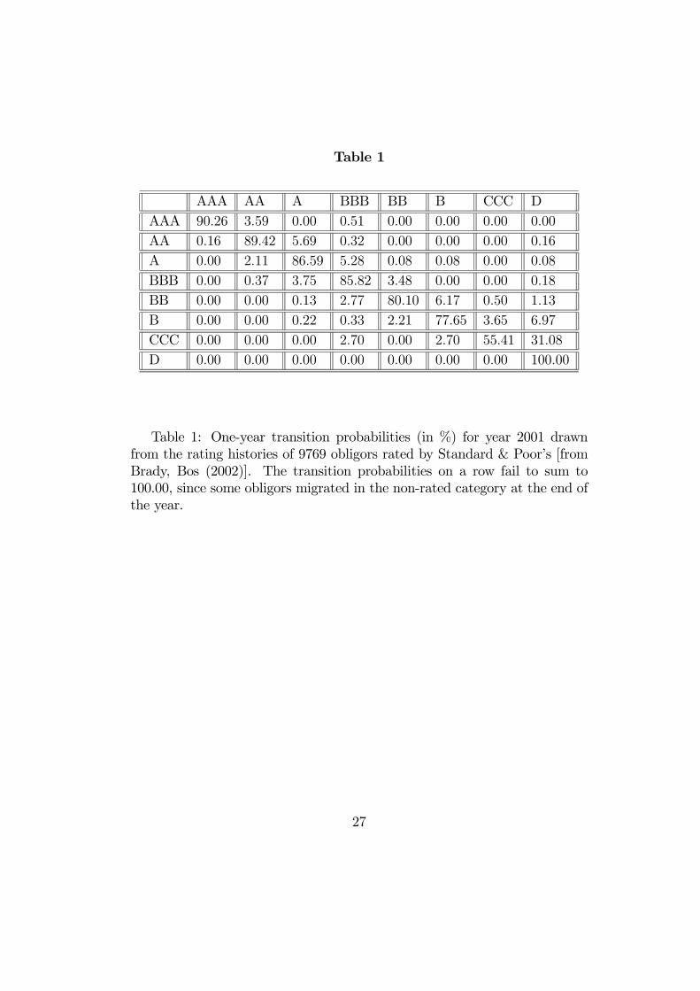
Table 1

AAA AA A BBB BB B CCC DAAA 90.26 3.59 0.00 0.51 0.00 0.00 0.00 0.00

AA 0.16 89.42 5.69 0.32 0.00 0.00 0.00 0.16

A 0.00 2.11 86.59 5.28 0.08 0.08 0.00 0.08

BBB 0.00 0.37 3.75 85.82 3.48 0.00 0.00 0.18

BB 0.00 0.00 0.13 2.77 80.10 6.17 0.50 1.13

B 0.00 0.00 0.22 0.33 2.21 77.65 3.65 6.97

CCC 0.00 0.00 0.00 2.70 0.00 2.70 55.41 31.08

D 0.00 0.00 0.00 0.00 0.00 0.00 0.00 100.00

Table 1: One-year transition probabilities (in %) for year 2001 drawnfrom the rating histories of 9769 obligors rated by Standard & Poor’s [fromBrady, Bos (2002)]. The transition probabilities on a row fail to sum to100.00, since some obligors migrated in the non-rated category at the end ofthe year.

27

Table 2

Mean (1, 1) (2, 2) (3, 3)

(1, 1) 0.633 0.112 0.000

(2, 2) 0.114 0.505 0.024

(3, 3) 0 0 1

Median (1, 1) (2, 2) (3, 3)

(1, 1) 0.635 0.108 0.000

(2, 2) 0.110 0.507 0.020

(3, 3) 0 0 1

Std. dev. (1, 1) (2, 2) (3, 3)

(1, 1) 0.069 0.040 0.001

(2, 2) 0.043 0.053 0.017

(3, 3) − − −

MSE (1, 1) (2, 2) (3, 3)

(1, 1) 0.005 0.002 0.000

(2, 2) 0.002 0.003 0.000

(3, 3) − − −

5% Interquantile (1, 1) (2, 2) (3, 3)

(1, 1) 0.517/0.744 0.053/0.182 0.000/0.001

(2, 2) 0.051/0.190 0.416/0.590 0.004/0.057

(3, 3) − − −

1% Interquantile (1, 1) (2, 2) (3, 3)

(1, 1) 0.462/0.782 0.035/0.225 0.000/0.004

(2, 2) 0.032/0.234 0.375/0.618 0.002/0.079

(3, 3) − − −

Table 2: Estimated joint transition probabilities using estimator bpkk∗,ll∗defined in (10). In the first four tables we report the average, the median,the standard deviation and the Mean Squared Error, respectively, of theestimator bpkk∗,ll∗ in the Monte-Carlo sample. The ranges between the 0.05and the 0.95, resp. 0.01 and 0.99, quantiles of the estimator are reported inthe last two tables. The rows correspond to the starting grades (k, k), thecolumns to the final grades (k∗, k∗), k, k∗ = 1, 2, 3.

28

Table 3

Mean (1, 1) (2, 2) (3, 3)

(1, 1) 0.634 0.109 0.000

(2, 2) 0.115 0.504 0.023

(3, 3) 0 0 1

Median (1, 1) (2, 2) (3, 3)

(1, 1) 0.710 0.024 0.000

(2, 2) 0.024 0.572 0.000

(3, 3) 0 0 1

Std. dev. (1, 1) (2, 2) (3, 3)

(1, 1) 0.306 0.173 0.006

(2, 2) 0.189 0.234 0.074

(3, 3) − − −

MSE (1, 1) (2, 2) (3, 3)

(1, 1) 0.093 0.030 0.000

(2, 2) 0.035 0.055 0.005

(3, 3) − − −

5% Interquantile (1, 1) (2, 2) (3, 3)

(1, 1) 0.064/0.997 0/0.534 0/0.000

(2, 2) 0/0.558 0.056/0.772 0/0.131

(3, 3) − − −

1% Interquantile (1, 1) (2, 2) (3, 3)

(1, 1) 0.007/1 0/0.726 0/0.002

(2, 2) 0/0.833 0.006/0.823 0/0.391

(3, 3) − − −

Table 3: Estimated joint transition probabilities using estimator bpkl,t de-fined in (1) at date t = 10. In the first four tables we report the average, themedian, the standard deviation and the Mean Squared Error, respectively, ofthe estimator bpkl,t in the Monte-Carlo sample. The range between the 0.05and the 0.95, resp. 0.01 and 0.99, quantiles of the estimator are reported inthe last two tables. The rows correspond to the starting grades (k, k), thecolumns to the final grades (l, l), k, l = 1, 2, 3.

29

Table 4

(1, 1) (2, 2) (3, 3)

(1, 1) 0.634 0.109 0.000

(2, 2) 0.113 0.505 0.023

(3, 3) 0 0 1

Table 4: Joint transition probabilities pkk∗,kk∗. The rows corresponds tothe starting grades (k, k), the columns to the final grades (k∗, k∗), k, k∗ =1, 2, 3.

30

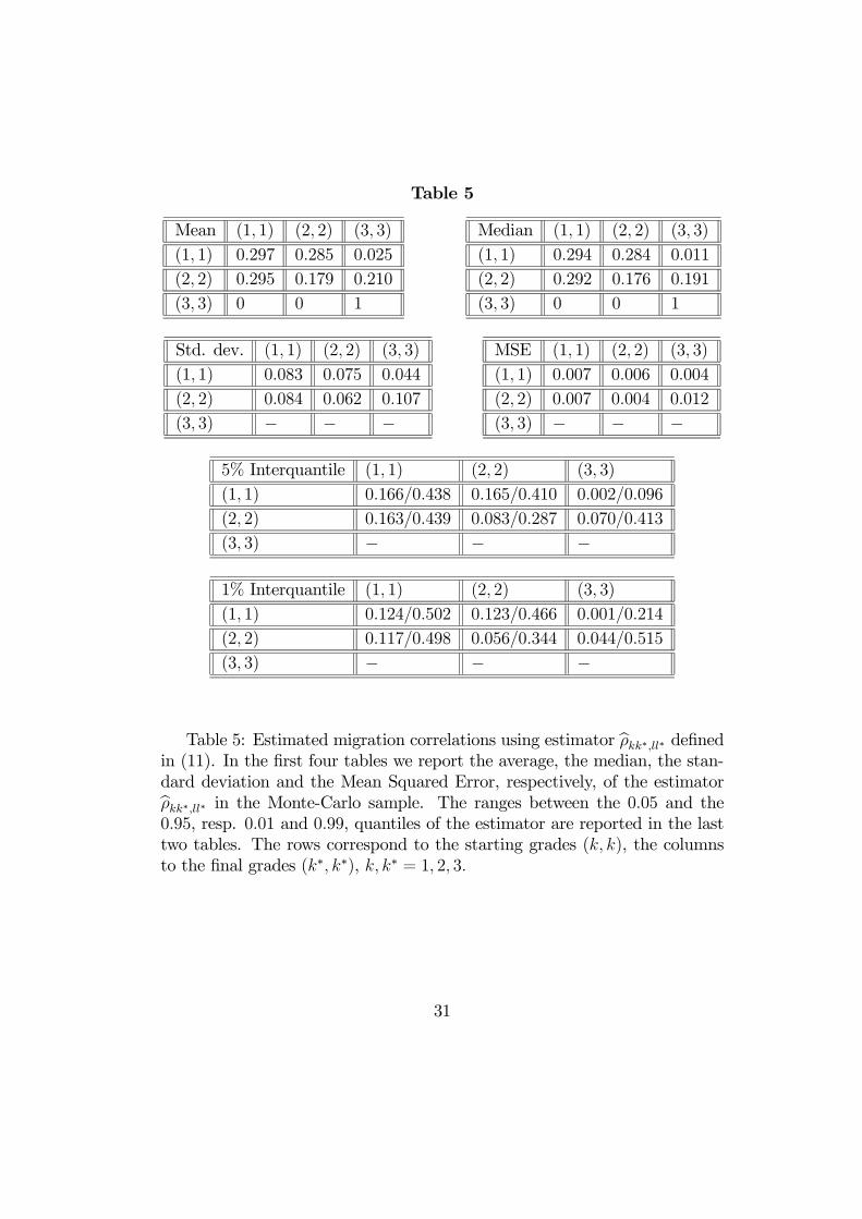
Table 5

Mean (1, 1) (2, 2) (3, 3)

(1, 1) 0.297 0.285 0.025

(2, 2) 0.295 0.179 0.210

(3, 3) 0 0 1

Median (1, 1) (2, 2) (3, 3)

(1, 1) 0.294 0.284 0.011

(2, 2) 0.292 0.176 0.191

(3, 3) 0 0 1

Std. dev. (1, 1) (2, 2) (3, 3)

(1, 1) 0.083 0.075 0.044

(2, 2) 0.084 0.062 0.107

(3, 3) − − −

MSE (1, 1) (2, 2) (3, 3)

(1, 1) 0.007 0.006 0.004

(2, 2) 0.007 0.004 0.012

(3, 3) − − −

5% Interquantile (1, 1) (2, 2) (3, 3)

(1, 1) 0.166/0.438 0.165/0.410 0.002/0.096

(2, 2) 0.163/0.439 0.083/0.287 0.070/0.413

(3, 3) − − −

1% Interquantile (1, 1) (2, 2) (3, 3)

(1, 1) 0.124/0.502 0.123/0.466 0.001/0.214

(2, 2) 0.117/0.498 0.056/0.344 0.044/0.515

(3, 3) − − −

Table 5: Estimated migration correlations using estimator bρkk∗,ll∗ definedin (11). In the first four tables we report the average, the median, the stan-dard deviation and the Mean Squared Error, respectively, of the estimatorbρkk∗,ll∗ in the Monte-Carlo sample. The ranges between the 0.05 and the0.95, resp. 0.01 and 0.99, quantiles of the estimator are reported in the lasttwo tables. The rows correspond to the starting grades (k, k), the columnsto the final grades (k∗, k∗), k, k∗ = 1, 2, 3.

31

Table 6

Mean (1, 1) (2, 2) (3, 3)

(1, 1) −0.007 −0.007 −0.007(2, 2) −0.007 −0.007 −0.007(3, 3) 0 0 1

Median (1, 1) (2, 2) (3, 3)

(1, 1) −0.003 −0.003 −0.003(2, 2) −0.003 −0.003 −0.003(3, 3) 0 0 1

Std. dev. (1, 1) (2, 2) (3, 3)

(1, 1) 0.029 0.029 0.029

(2, 2) 0.026 0.026 0.026

(3, 3) − − −

MSE (1, 1) (2, 2) (3, 3)

(1, 1) 0.099 0.091 0.007

(2, 2) 0.098 0.037 0.058

(3, 3) − − −

5% Interquantile (1, 1) (2, 2) (3, 3)

(1, 1) −0.019/− 0.001 −0.019/− 0.001 −0.019/− 0.001(2, 2) −0.019/− 0.002 −0.019/− 0.002 −0.019/− 0.002(3, 3) − − −

1% Interquantile (1, 1) (2, 2) (3, 3)

(1, 1) −0.067/− 0.001 −0.067/− 0.001 −0.067/− 0.001(2, 2) −0.063/− 0.001 −0.063/− 0.001 −0.063/− 0.001(3, 3) − − −

Table 6: Estimated migration correlations using estimator bρkl,t definedin (2) at date t = 10. In the first four tables we report the average, themedian, the standard deviation and the Mean Squared Error, respectively, ofthe estimator bρkl,t in the Monte-Carlo sample. The range between the 0.05and the 0.95, resp. 0.01 and 0.99, quantiles of the estimator are reported inthe last two tables. The rows correspond to the starting grades (k, k), thecolumns to the final grades (l, l), k, l = 1, 2, 3.

32

Table 7

(1, 1) (2, 2) (3, 3)

(1, 1) 0.305 0.293 0.072

(2, 2) 0.305 0.184 0.232

(3, 3) − − −

Table 7: Migration correlations ρkk∗,kk∗ . The rows corresponds to thestarting grades (k, k), the columns to the final grades (k∗, k∗), k, k∗ = 1, 2, 3.

33

Table 8

Mean (1, 1) (2, 2) (3, 3)

(1, 1) 0.268 0.174 0.058

(2, 2) 0.201 0.136 0.137

(3, 3) 0 0 1

Median (1, 1) (2, 2) (3, 3)

(1, 1) 0.255 0.176 0.035(2, 2) 0.182 0.137 0.103(3, 3) 0 0 1

Std. dev. (1, 1) (2, 2) (3, 3)

(1, 1) 0.129 0.048 0.065

(2, 2) 0.118 0.039 0.102

(3, 3) − − −

MSE (1, 1) (2, 2) (3, 3)

(1, 1) 0.017 0.002 0.004

(2, 2) 0.014 0.002 0.010

(3, 3) − − −

5% Interquantile (1, 1) (2, 2) (3, 3)

(1, 1) 0.081/0.499 0.091/0.251 0.003/0.193

(2, 2) 0.043/0.423 0.070/0.200 0.017/0.340

(3, 3) − − −

1% Interquantile (1, 1) (2, 2) (3, 3)

(1, 1) 0.040/0.606 0.060/0.279 0.001/0.300

(2, 2) 0.019/0.540 0.046/0.223 0.006/0.454

(3, 3) − − −

Table 8: Estimated joint transition probabilities at horizon h = 7 usingestimator epkk∗,ll∗(7) defined in (13). In the first four tables we report theaverage, the median, the standard deviation and the Mean Squared Error,respectively, of the estimator epkk∗,ll∗(7) in the Monte-Carlo sample. Theranges between the 0.05 and the 0.95, resp. 0.01 and 0.99, quantiles ofthe estimator are reported in the last two tables. In each table the rowscorrespond to the starting grades (k, k), the columns to the final grades(k∗, k∗), k, k∗ = 1, 2, 3.

34

Table 9

Mean (1, 1) (2, 2) (3, 3)

(1, 1) 0.277 0.168 0.066(2, 2) 0.213 0.131 0.137(3, 3) 0 0 1

Median (1, 1) (2, 2) (3, 3)

(1, 1) 0.268 0.169 0.051

(2, 2) 0.201 0.131 0.120

(3, 3) 0 0 1

Std. dev. (1, 1) (2, 2) (3, 3)

(1, 1) 0.110 0.031 0.057

(2, 2) 0.102 0.023 0.089

(3, 3) − − −

MSE (1, 1) (2, 2) (3, 3)

(1, 1) 0.012 0.001 0.003

(2, 2) 0.011 0.001 0.008

(3, 3) − − −

5% Interquantile (1, 1) (2, 2) (3, 3)

(1, 1) 0.114/0.476 0.115/0.218 0.007/0.181

(2, 2) 0.072/0.404 0.095/0.170 0.025/0.311

(3, 3) − − −

1% Interquantile (1, 1) (2, 2) (3, 3)

(1, 1) 0.072/0.569 0.086/0.239 0.002/0.256

(2, 2) 0.043/0.502 0.078/0.189 0.011/0.404

(3, 3) − − −

Table 9: Estimated joint transition probabilities at horizon h = 7 usingestimator bpkk∗,ll∗(7) defined in (14). In the first four tables we report theaverage, the median, the standard deviation and the Mean Squared Error,respectively, of the estimator bpkk∗,ll∗(7) in the Monte-Carlo sample. Theranges between the 0.05 and the 0.95, resp. 0.01 and 0.99, quantiles ofthe estimator are reported in the last two tables. In each table the rowscorrespond to the starting grades (k, k), the columns to the final grades(k∗, k∗), k, k∗ = 1, 2, 3.

35

Table 10

(1, 1) (2, 2) (3, 3)

(1, 1) 0.265 0.173 0.058

(2, 2) 0.198 0.135 0.131

(3, 3) 0 0 1

Table 10: Joint transition probabilities pkk∗,ll∗(7) at horizon h = 7. Therows corresponds to the starting grades (k, k), the columns to the final grades(k∗, k∗), k, k∗ = 1, 2, 3.

36

Table 11

Mean (1, 1) (2, 2) (3, 3)

(1, 1) 0.200 0.134 0.096

(2, 2) 0.172 0.128 0.126

(3, 3) 0 0 1

Median (1, 1) (2, 2) (3, 3)

(1, 1) 0.186 0.127 0.068

(2, 2) 0.157 0.121 0.103

(3, 3) 0 0 1

Std. dev. (1, 1) (2, 2) (3, 3)

(1, 1) 0.089 0.059 0.089

(2, 2) 0.083 0.058 0.092

(3, 3) − − −

MSE (1, 1) (2, 2) (3, 3)

(1, 1) 0.011 0.004 0.015

(2, 2) 0.011 0.003 0.014

(3, 3) − − −

5% Interquantile (1, 1) (2, 2) (3, 3)

(1, 1) 0.081/0.365 0.049/0.241 0.012/0.277

(2, 2) 0.064/0.331 0.049/0.236 0.027/0.307

(3, 3) − − −

1% Interquantile (1, 1) (2, 2) (3, 3)

(1, 1) 0.053/0.465 0.030/0.297 0.006/0.421

(2, 2) 0.042/0.422 0.030/0.294 0.015/0.445

(3, 3)

Table 11: Estimated migration correlations at horizon h = 7 using estima-tor eρkk∗,ll∗(7) defined in (15). In the first four tables we report the average, themedian, the standard deviation and the Mean Squared Error, respectively,of the estimator epkk∗,ll∗(7) in the Monte-Carlo sample. The ranges betweenthe 0.05 and the 0.95, resp. 0.01 and 0.99, quantiles of the estimator arereported in the last two tables. In each table the rows correspond to thestarting grades (k, k), the columns to the final grades (k∗, k∗), k, k∗ = 1, 2, 3.

37

Table 12

Mean (1, 1) (2, 2) (3, 3)

(1, 1) 0.243 0.143 0.159

(2, 2) 0.222 0.135 0.179

(3, 3) 0 0 1

Median (1, 1) (2, 2) (3, 3)

(1, 1) 0.243 0.142 0.149

(2, 2) 0.220 0.134 0.168

(3, 3) 0 0 1

Std. dev. (1, 1) (2, 2) (3, 3)

(1, 1) 0.053 0.040 0.074

(2, 2) 0.051 0.037 0.077

(3, 3) − − −

MSE (1, 1) (2, 2) (3, 3)

(1, 1) 0.003 0.002 0.006

(2, 2) 0.003 0.001 0.007

(3, 3) − − −

5% Interquantile (1, 1) (2, 2) (3, 3)

(1, 1) 0.155/0.331 0.079/0.211 0.053/0.293

(2, 2) 0.142/0.309 0.077/0.198 0.071/0.320

(3, 3) − − −

1% Interquantile (1, 1) (2, 2) (3, 3)

(1, 1) 0.121/0.368 0.057/0.242 0.030/0.356

(2, 2) 0.111/0.351 0.056/0.230 0.045/0.393

(3, 3) − − −

Table 12: Estimated migration correlations at horizon h = 7 using estima-tor bρkk∗,ll∗(7) defined in (16). In the first four tables we report the average, themedian, the standard deviation and the Mean Squared Error, respectively,of the estimator bρkk∗,ll∗(7) in the Monte-Carlo sample. The ranges betweenthe 0.05 and the 0.95, resp. 0.01 and 0.99, quantiles of the estimator arereported in the last two tables. In each table the rows correspond to thestarting grades (k, k), the columns to the final grades (k∗, k∗), k, k∗ = 1, 2, 3.

38

Table 13

(1, 1) (2, 2) (3, 3)

(1, 1) 0.257 0.145 0.182

(2, 2) 0.236 0.136 0.203

(3, 3) 0 0 1

Table 13: Migration correlations ρkk∗,ll∗(7) at horizon h = 7. The rowscorresponds to the starting grades (k, k), the columns to the final grades(k∗, k∗), k, k∗ = 1, 2, 3.

39

Figure 1: Rating histories of two firms.

40

Figure 2: Histogram of S = 10000 Monte-Carlo replications of the estimatorbpkk∗,ll∗ in (10). From left to right and top to bottom, the four panels reportthe estimators for k = l = 1, k∗ = l∗ = 2 (joint downgrade), k = l = 1, k∗ =l∗ = 3 (joint default starting from the best rating) k = l = 2, k∗ = l∗ = 1(joint upgrade), and k = l = 2, k∗ = l∗ = 3 (joint default starting from theworst rating). 41

Figure 3: Histogram of S = 10000 Monte-Carlo replications of the estimatorbpkl,t in ( 1) for t = 10. From left to right and top to bottom, the fourpanels report the estimators for k = 1, l = 2 (joint downgrade), k = 1, l = 3(joint default starting from the best rating) k = 2, l = 1 (joint upgrade), andk = 2, l = 3 (joint default starting from the worst rating).

42

Figure 4: Histogram of S = 10000 Monte-Carlo replications of the estimatorepkl,kl(7) in (13). From left to right and top to bottom, the four panels reportthe estimators for k = 1, l = 2 (joint downgrade), k = 1, l = 3 (joint defaultstarting from the best rating) k = 2, l = 1 (joint upgrade), and k = 2, l = 3(joint default starting from the worst rating).

43

Figure 5: Histogram of S = 10000 Monte-Carlo replications of the estimatorbpkl,kl(7) in (14). From left to right and top to bottom, the four panels reportthe estimators for k = 1, l = 2 (joint downgrade), k = 1, l = 3 (joint defaultstarting from the best rating) k = 2, l = 1 (joint upgrade), and k = 2, l = 3(joint default starting from the worst rating).

44

Figure 6: Histogram of S = 10000 Monte-Carlo replications of the estimatoreρkl,kl(7) in (15). From left to right and top to bottom, the four panels reportthe estimators for k = 1, l = 2 (joint downgrade), k = 1, l = 3 (joint defaultstarting from the best rating) k = 2, l = 1 (joint upgrade), and k = 2, l = 3(joint default starting from the worst rating).

45

Figure 7: Histogram of S = 10000 Monte-Carlo replications of the estimatorbρkl,kl(7) in (16). From left to right and top to bottom, the four panels reportthe estimators for k = 1, l = 2 (joint downgrade), k = 1, l = 3 (joint defaultstarting from the best rating) k = 2, l = 1 (joint upgrade), and k = 2, l = 3(joint default starting from the worst rating).

46