migration and attenuation of surface-related and interbed multiple reflections
DESCRIPTION
Migration and Attenuation of Surface-Related and Interbed Multiple Reflections. Zhiyong Jiang. University of Utah. April 21, 2006. Outline. Overview Surface Multiple Migration Interbed Multiple Migration Multiple Attenuation in Multiple Imaging Conclusions. - PowerPoint PPT PresentationTRANSCRIPT

Migration and Attenuation of Migration and Attenuation of Surface-Related and Interbed Surface-Related and Interbed
Multiple ReflectionsMultiple Reflections
Zhiyong JiangZhiyong Jiang
University of UtahUniversity of Utah
April 21, 2006April 21, 2006

OutlineOutline• OverviewOverview• Surface Multiple Migration Surface Multiple Migration • Interbed Multiple MigrationInterbed Multiple Migration• Multiple Attenuation inMultiple Attenuation in Multiple ImagingMultiple Imaging• ConclusionsConclusions
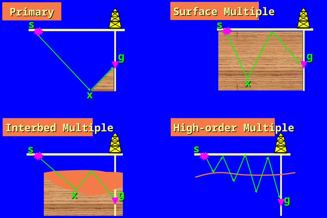
gg
ss
xx
PrimaryPrimary
gg
ss
xx
Surface MultipleSurface Multiple
gg
ss
xx
Interbed MultipleInterbed Multiple
gg
ss
High-order MultipleHigh-order Multiple
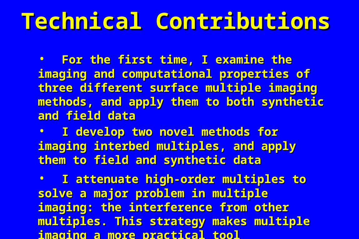
• For the first time, I examine the imaging and For the first time, I examine the imaging and computational properties of three different surface computational properties of three different surface multiple imaging methods, and apply them to both multiple imaging methods, and apply them to both synthetic and field datasynthetic and field data
Technical ContributionsTechnical Contributions
• I develop two novel methods for imaging interbed I develop two novel methods for imaging interbed multiples, and apply them to field and synthetic datamultiples, and apply them to field and synthetic data
• I attenuate high-order multiples to solve a major I attenuate high-order multiples to solve a major problem in multiple imaging: the interference from problem in multiple imaging: the interference from other multiples. This strategy makes multiple other multiples. This strategy makes multiple imaging a more practical toolimaging a more practical tool
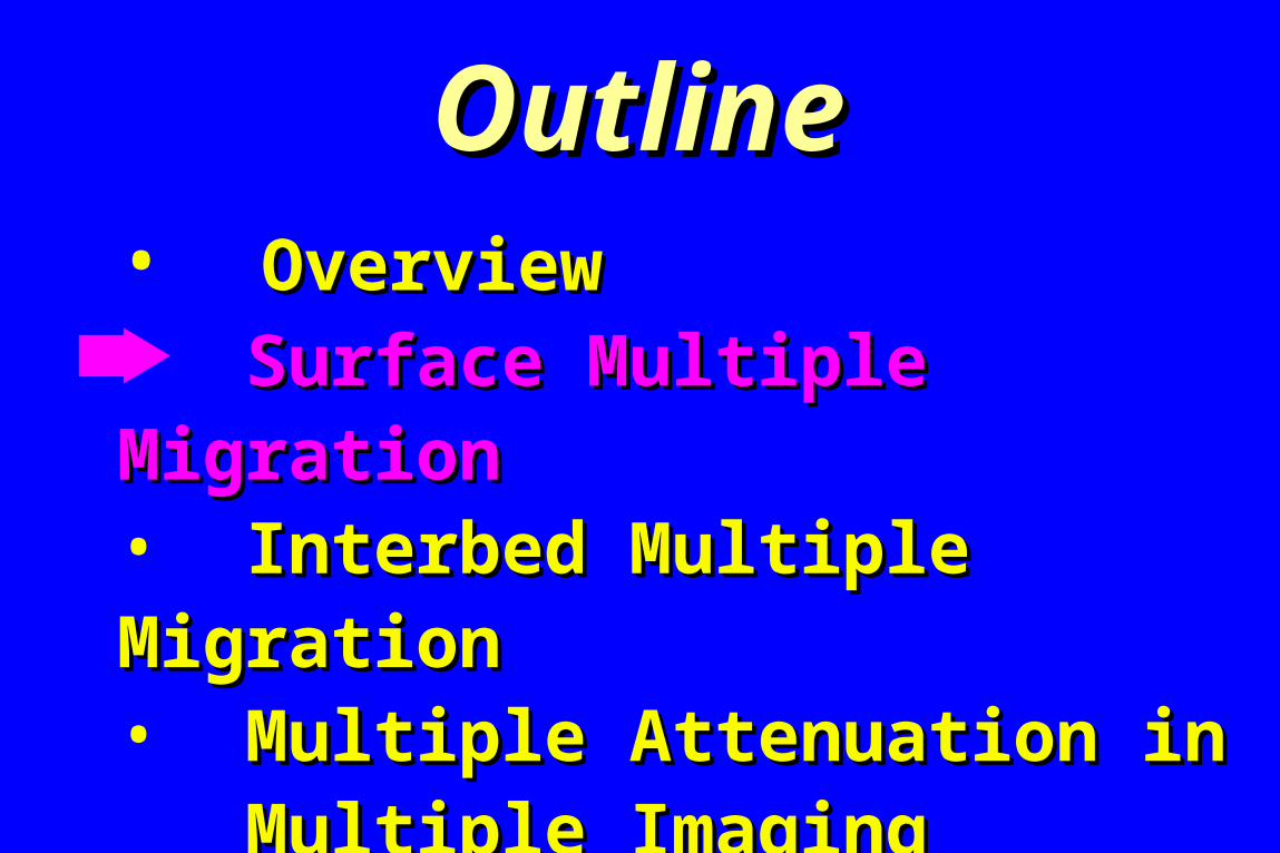
OutlineOutline• OverviewOverview• Surface Multiple Migration Surface Multiple Migration • Interbed Multiple MigrationInterbed Multiple Migration• Multiple Attenuation inMultiple Attenuation in Multiple ImagingMultiple Imaging• ConclusionsConclusions

OutlineOutline• OverviewOverview• Surface Multiple Migration Surface Multiple Migration
• MotivationMotivation• Methodology Methodology • Numerical ResultsNumerical Results• Summary Summary

Why Migrate Surface Multiples?Why Migrate Surface Multiples?
Better FoldBetter Fold
Better Vert. Res.Better Vert. Res.
Wider CoverageWider Coverage

Shot radius
Z
3D VSP3D VSP SurveySurvey

OutlineOutline• OverviewOverview• Surface Multiple Migration Surface Multiple Migration
• MotivationMotivation• MethodologyMethodology • Numerical ResultsNumerical Results• Summary Summary
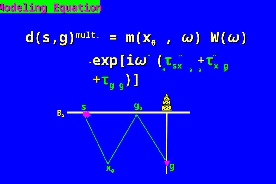
gg
ss
xx00
gg00BB00
d(s,g)d(s,g)mult.mult. = m(x = m(x00 , , ωω) W() W(ωω))
exp[iexp[iωω ( (ττsxsx ++ττx gx g ++ττg gg g)] )] 00 00 0000
..~~ ~~ ~~
Modeling EquationModeling Equation
gg
ss
xx
g’g’00BB00
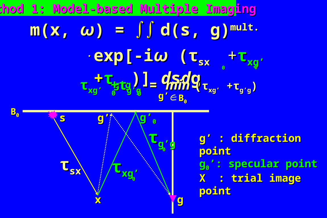
Method 1: Model-based Multiple ImagingMethod 1: Model-based Multiple Imaging
m(x, m(x, ωω) = ) = ∫∫ ∫∫ d(s, g)d(s, g)mult.mult.
exp[-iexp[-iωω ( (ττsx sx ++ττxg’xg’ ++ττg’gg’g)] )] ddssddg g 0000
..
ττsxsx ττxg’xg’00
ττg’gg’g00
ττxg’xg’ ++ττg’gg’g = = min min ((ττxg’xg’ ++ττg’gg’g))g’g’ BB00
00 00
g’g’
g’ : diffraction pointg’ : diffraction pointgg00’: specular point’: specular point
X : trial image pointX : trial image point
gg
ss
xx
g’g’00BB00
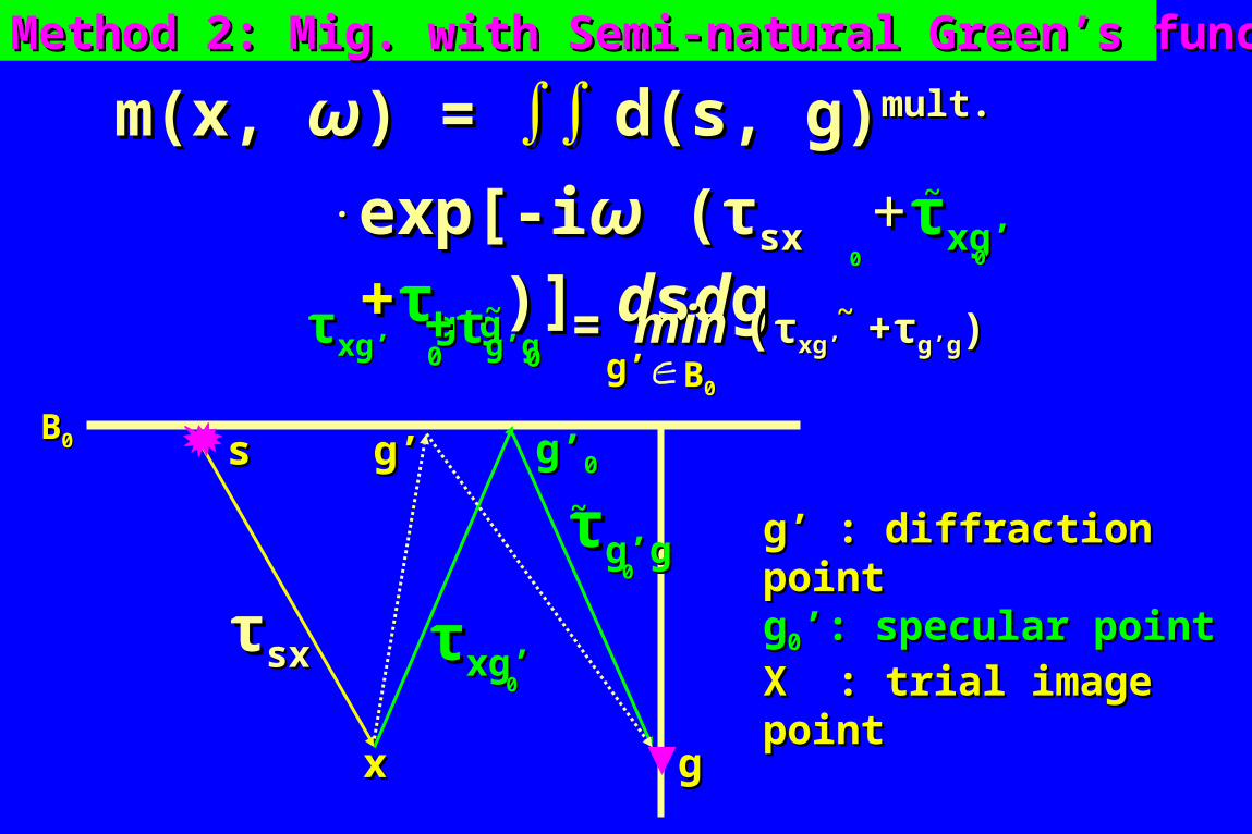
Method 2: Mig. with Semi-natural Green’s functionsMethod 2: Mig. with Semi-natural Green’s functions
m(x, m(x, ωω) = ) = ∫∫ ∫∫ d(s, g)d(s, g)mult.mult.
exp[-iexp[-iωω ( (ττsx sx ++ττxg’xg’ ++ττg’gg’g)] )] ddssddg g 0000
..
ττxg’xg’ ++ττg’gg’g = = min min ((ττxg’xg’ ++ττg’gg’g))g’g’ BB00
00 00
g’g’
g’ : diffraction pointg’ : diffraction pointgg00’: specular point’: specular point
X : trial image pointX : trial image point
~~
~~ ~~
ττsxsx ττxg’xg’
ττg’gg’g
00
~~
00
gg
ss
xx
BB00
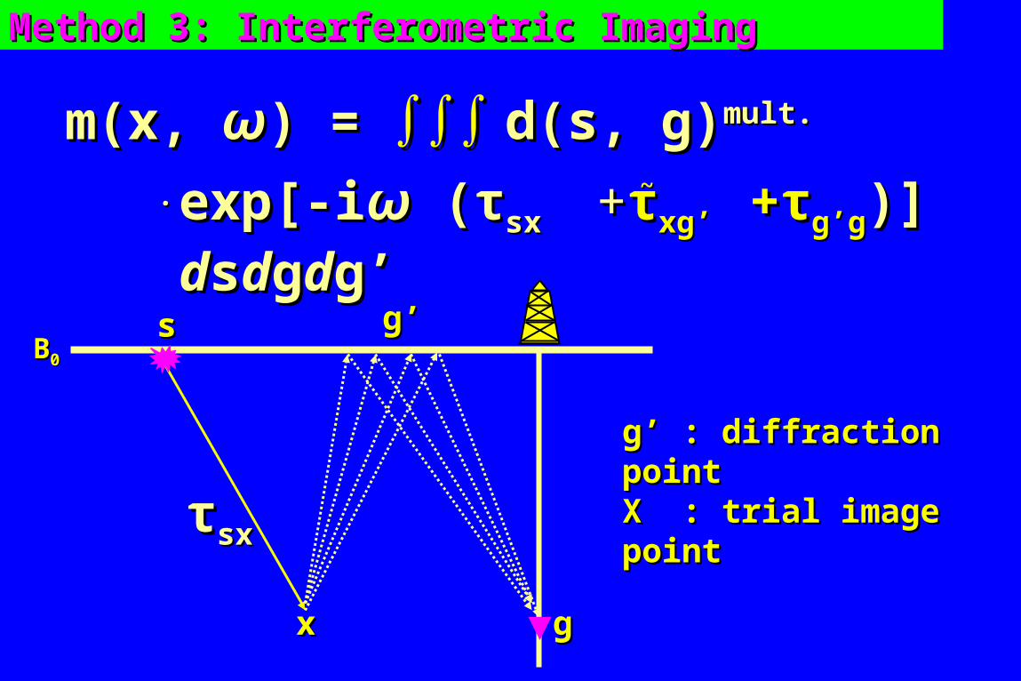
Method 3: Interferometric ImagingMethod 3: Interferometric Imaging
m(x, m(x, ωω) = ) = ∫∫∫ ∫∫∫ d(s, g)d(s, g)mult.mult.
exp[-iexp[-iωω ( (ττsx sx ++ττxg’ xg’ ++ττg’gg’g)] )] ddssddggddg’ g’ ..
g’g’
g’ : diffraction pointg’ : diffraction pointX : trial image pointX : trial image point
~~
ττsxsx

MigrationMigration
MethodsMethods
Sensitivity Sensitivity to velocity to velocity errors errors
Receiver Receiver Statics in Statics in VSP case VSP case eliminated?eliminated?
Receiver Receiver geometry geometry needs to be needs to be known in known in VSP case?VSP case?
Coverage Coverage in VSP in VSP casecase
Applicablbe Applicablbe to to IVSPWD?IVSPWD?
Model-based Model-based multiple multiple MigrationMigration
High No Yes Wide No
Semi-natural Semi-natural Green’s Green’s functionsfunctions
Low Yes No Wide No
Interferomet-Interferomet-ric Imagingric Imaging
Low Yes No Wide Yes
Primary Primary MigrationMigration
Low No Yes Narrow No
Imaging Properties of Migration MethodsImaging Properties of Migration Methods
OutlineOutline• OverviewOverview• Surface Multiple Migration Surface Multiple Migration
• MotivationMotivation• Methodology Methodology • Numerical ResultsNumerical Results• Summary Summary

Numerical ResultsNumerical Results
• 2-D Dipping Layer Model2-D Dipping Layer Model
• 3-D Real Data3-D Real Data
• 3-D Synthetic Data3-D Synthetic Data

Velocity ModelVelocity Model
00
13001300
92592500 X (m)X (m)
Dep
th (
m)
Dep
th (
m)
19001900
40004000V (m/s)V (m/s)
Shots: 92; Receivers: 91 (50m -950 m)Shots: 92; Receivers: 91 (50m -950 m)
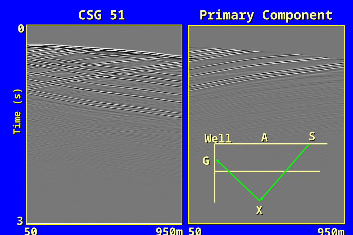
WellWell

CSG 51CSG 51
5050 950m950m 950m950m5050
Tim
e (s
)T
ime
(s)
33
00Ghost ComponentGhost Component
SS
GG
XX
AAWellWell
CSG 51CSG 51
5050 950m950m 950m950m5050
Tim
e (s
)T
ime
(s)
33
00Primary ComponentPrimary Component
SS
GG
XX
AAWellWell

X (m)X (m)00 925925
00
13001300
Dep
th (
m)
Dep
th (
m)
X (m)X (m) 92592500
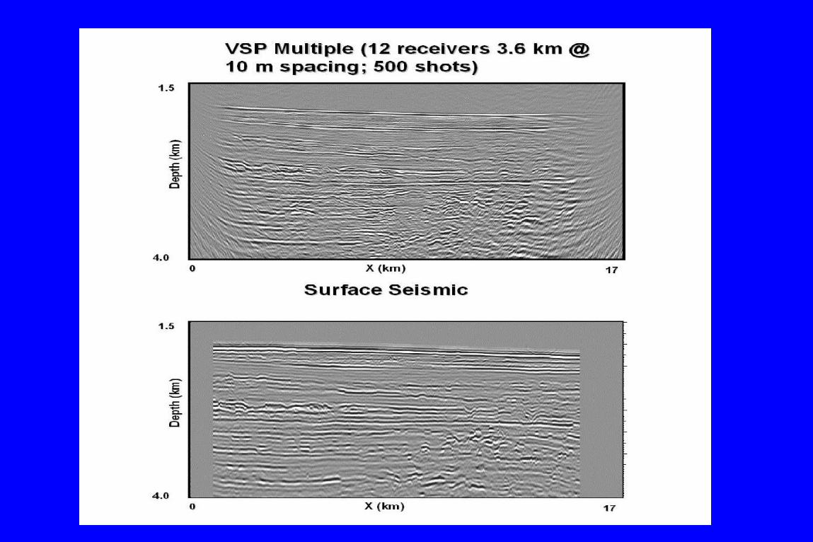
PrimaryPrimary 1st-order multiple 1st-order multiple 8 Receivers8 Receivers
Numerical ResultsNumerical Results
• 2-D Dipping Layer Model2-D Dipping Layer Model
• 3-D Real Data3-D Real Data
• 3-D Synthetic Data3-D Synthetic Data

Numerical ResultsNumerical Results
• 2-D Dipping Layer Model2-D Dipping Layer Model
• 3-D Real Data3-D Real Data
• 3-D Synthetic Data 3-D Synthetic Data
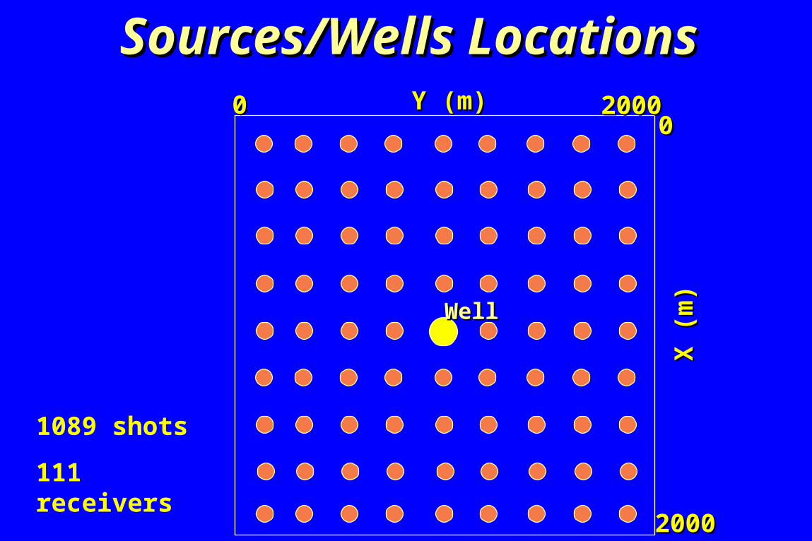
Y (m)Y (m)00 2000200000
X (
m)
X (
m)
20002000
1089 shots
111 receivers
WellWell
Sources/Wells LocationsSources/Wells Locations

CSG10 CSG10
11 111111 11111111
Tim
e (s
)T
ime
(s)
3.53.5
00
XX
CSG540CSG540
Receiver NumberReceiver Number Receiver NumberReceiver Number

100100
11001100
Dep
th (
m)
Dep
th (
m)
PrimaryPrimary
Velocity ModelVelocity Model
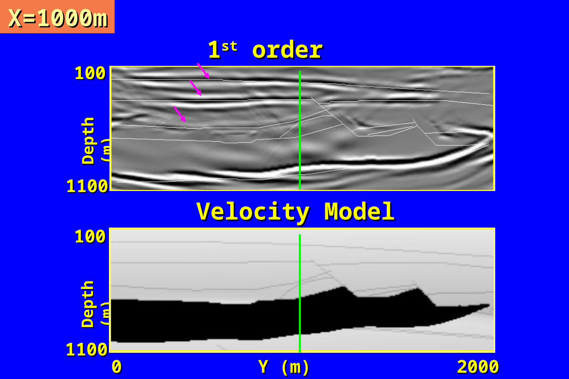
X=1000mX=1000m
Y (m)Y (m)00 20002000
100100
11001100
Dep
th (
m)
Dep
th (
m)
100100
11001100
Dep
th (
m)
Dep
th (
m)
11stst order ghost order ghost
Velocity ModelVelocity Model
X=1000mX=1000m
Y (m)Y (m)00 20002000
100100
11001100
Dep
th (
m)
Dep
th (
m)

100100
11001100
Dep
th (
m)
Dep
th (
m)
PrimaryPrimary
Velocity ModelVelocity Model
Y=1000mY=1000m
X (m)X (m)00 20002000
100100
11001100
Dep
th (
m)
Dep
th (
m)

100100
11001100
Dep
th (
m)
Dep
th (
m)
11stst order ghost order ghost
Velocity ModelVelocity Model
Y=1000mY=1000m
X (m)X (m)00 20002000
100100
11001100
Dep
th (
m)
Dep
th (
m)
OutlineOutline• OverviewOverview• Surface Multiple Migration Surface Multiple Migration
• MotivationMotivation• Methodology Methodology • Numerical ResultsNumerical Results• SummarySummary
SummarySummary
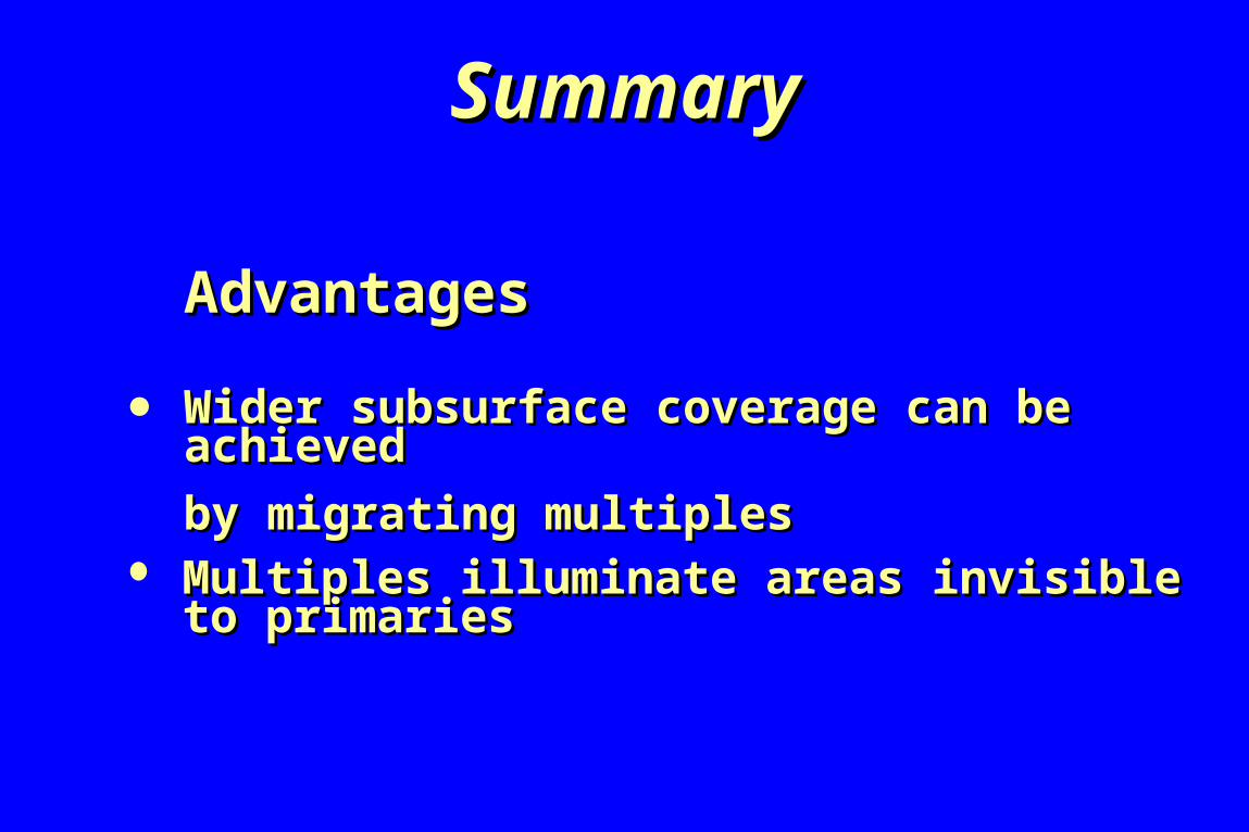
Wider subsurface coverage can be achievedWider subsurface coverage can be achieved
by migrating multiplesby migrating multiples
Multiples illuminate areas invisible to primariesMultiples illuminate areas invisible to primaries
AdvantagesAdvantages
SummarySummary
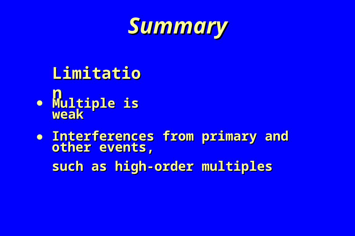
Multiple is weakMultiple is weak
Interferences from primary and other events, Interferences from primary and other events,
such as high-order multiplessuch as high-order multiples
LimitationLimitation

OutlineOutline• OverviewOverview• Surface Multiple Migration Surface Multiple Migration • Interbed Multiple MigrationInterbed Multiple Migration• Multiple Attenuation inMultiple Attenuation in Multiple ImagingMultiple Imaging• ConclusionsConclusions

OutlineOutline• OverviewOverview• Interbed Multiple Migration Interbed Multiple Migration
• MotivationMotivation• MethodsMethods• Numerical TestsNumerical Tests• Summary Summary
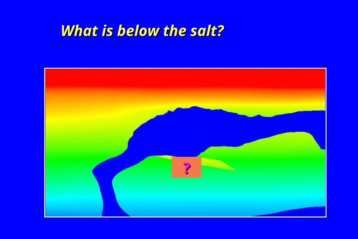
??
What is below the salt?What is below the salt?
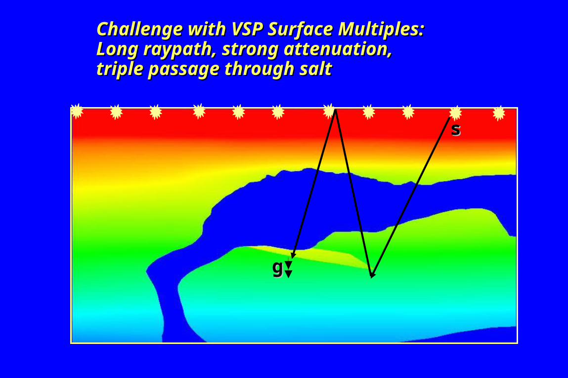
Challenge with VSP Surface Multiples: Challenge with VSP Surface Multiples: Long raypath, strong attenuation, Long raypath, strong attenuation, triple passage through salttriple passage through salt
gg
ss

Challenge with CDP primary reflections:Challenge with CDP primary reflections:strong attenuation, strong attenuation, double passage through salt double passage through salt
ssgg
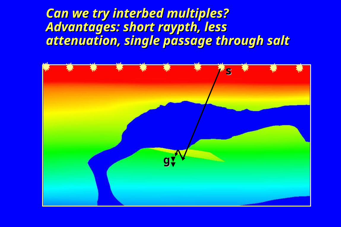
Can we try interbed multiples?Can we try interbed multiples?Advantages: short raypth, less Advantages: short raypth, less attenuation, single passage through saltattenuation, single passage through salt
gg
ss

OutlineOutline• OverviewOverview• Interbed Multiple Migration Interbed Multiple Migration
• MotivationMotivation• MethodsMethods• Numerical TestsNumerical Tests• Summary Summary
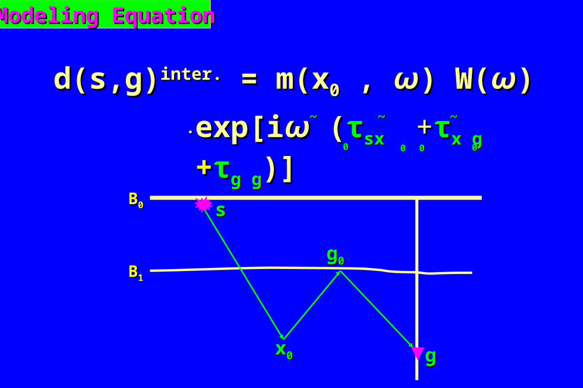
gg
ss
xx00
gg00
BB00
BB11
Modeling EquationModeling Equation
d(s,g)d(s,g)inter.inter. = m(x = m(x00 , , ωω) W() W(ωω))
exp[iexp[iωω ( (ττsx sx ++ττx gx g ++ττg gg g)] )] 00 00 0000
..~~ ~~ ~~

gg
ss
xx
g’g’00
BB00
BB11
Method 1: Fermat’s principleMethod 1: Fermat’s principle
m(x, m(x, ωω) = ) = ∫∫ ∫∫ d(s, g)d(s, g)inter.inter.
exp[-iexp[-iωω ( (ττsx sx ++ττxg’xg’ ++ττg’gg’g)] )] ddssddg g 0000
..
ττsxsx
ττxg’xg’00
ττg’gg’g00
ττxg’xg’ ++ττg’gg’g = = min min ((ττxg’xg’ ++ττg’gg’g))g’g’ BB11
00 00
g’g’
gg
ss
xx
BB00
BB11
g’g’
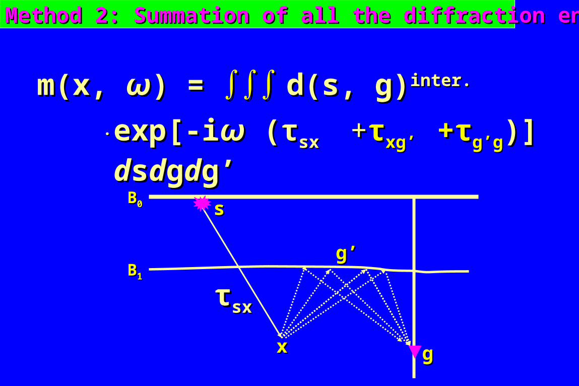
Method 2: Summation of all the diffraction energyMethod 2: Summation of all the diffraction energy
m(x, m(x, ωω) = ) = ∫∫∫ ∫∫∫ d(s, g)d(s, g)inter.inter.
exp[-iexp[-iωω ( (ττsx sx ++ττxg’ xg’ ++ττg’gg’g)] )] ddssddggddg’ g’ ..
ττsxsx
OutlineOutline• OverviewOverview• Interbed Multiple Migration Interbed Multiple Migration
• MotivationMotivation• MethodsMethods• Numerical TestsNumerical Tests• Summary Summary

Numerical TestsNumerical Tests
• SEG/EAGE ModelSEG/EAGE Model• Large Salt ModelLarge Salt Model• Field Data TestField Data Test
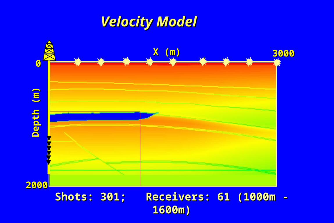
00
20002000
Dep
th (
m)
Dep
th (
m)
30003000X (m)X (m)
Shots: 301; Receivers: 61 (1000m - 1600m)Shots: 301; Receivers: 61 (1000m - 1600m)
Velocity ModelVelocity Model

00
20002000
Dep
th (
m)
Dep
th (
m)
3000300000 X (m)X (m)
ss
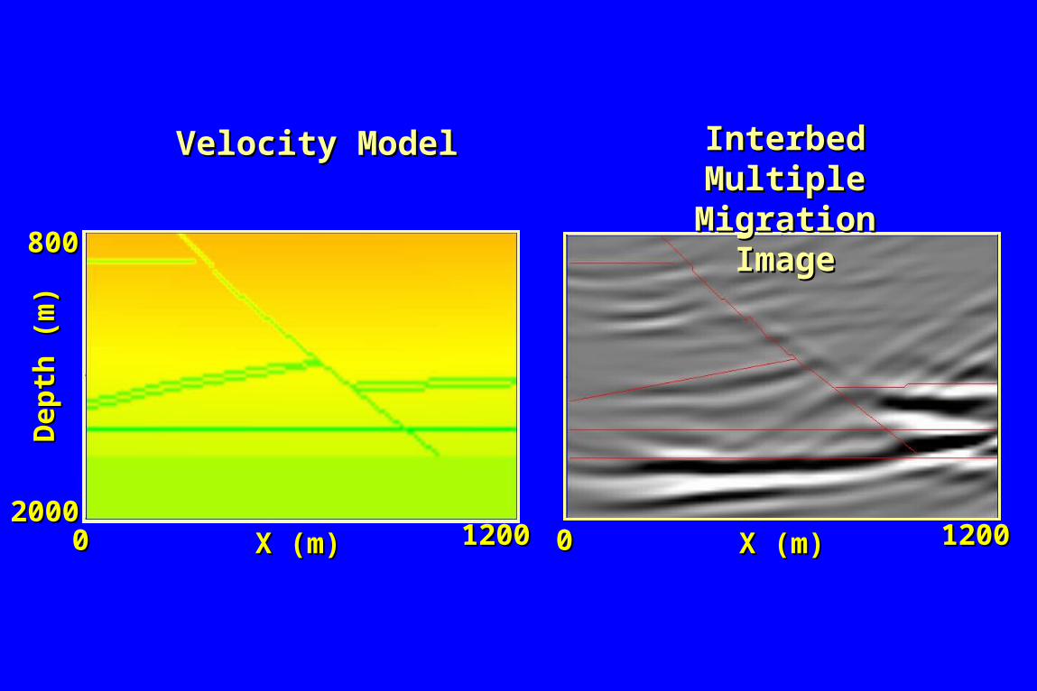
Upper-salt-boundary Interbed MultipleUpper-salt-boundary Interbed Multiple
xx
g’g’00
gg

Interbed Multiple Interbed Multiple Migration ImageMigration Image
1200120000 X (m)X (m)
800800
20002000
Dep
th (
m)
Dep
th (
m)
1200120000 X (m)X (m)
Velocity ModelVelocity Model
00
20002000
Dep
th (
m)
Dep
th (
m)
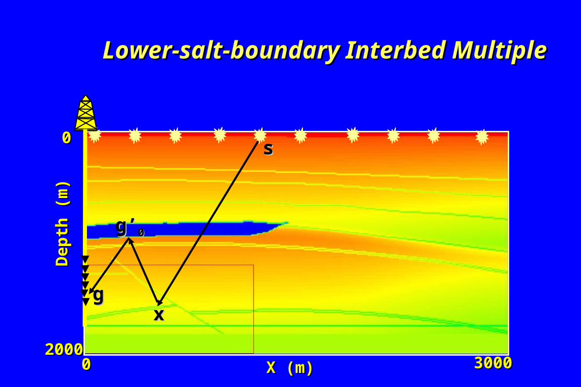
3000300000 X (m)X (m)
ss
Lower-salt-boundary Interbed MultipleLower-salt-boundary Interbed Multiple
xx
g’g’00
gg
00
800800
20002000
Dep
th (
m)
Dep
th (
m)
12001200X (m)X (m) 00 12001200X (m)X (m)
Velocity ModelVelocity Model Interbed Multiple Interbed Multiple Migration ImageMigration Image

Numerical TestsNumerical Tests
• SEG/EAGE ModelSEG/EAGE Model• Large Salt ModelLarge Salt Model• Field Data TestField Data Test

160001600000 X (m)X (m)00
1100011000
Dep
th (
m)
Dep
th (
m)Velocity ModelVelocity Model
Shots: 319; Receivers: 21Shots: 319; Receivers: 21

160001600000 X (m)X (m)
00
1100011000
Dep
th (
m)
Dep
th (
m)
Lower-salt-boundary Interbed MultipleLower-salt-boundary Interbed Multiple
ss
xxgg
g’g’00

00 12001200X (m)X (m)
62506250
72507250
Dep
th (
m)
Dep
th (
m)
00
62506250
72507250
Dep
th (
m)
Dep
th (
m)
12001200X (m)X (m)
Velocity ModelVelocity Model
Interbed Multiple Migration ImageInterbed Multiple Migration Image

Numerical TestsNumerical Tests
• SEG/EAGE ModelSEG/EAGE Model• Large Salt ModelLarge Salt Model• Field Data TestField Data Test

00
1066810668
Dep
th (
m)
Dep
th (
m)
16000m16000m00
Shots: 102; Receivers: 12Shots: 102; Receivers: 12
Velocity ModelVelocity Model

00
1066810668
Dep
th (
m)
Dep
th (
m)
16000m16000m00
Sea-bed Interbed MultipleSea-bed Interbed Multiple
ss
gg
g’g’00
xx

4000400000 X (m)X (m)40004000
Dep
th (
m)
Dep
th (
m)
20002000
40004000
Dep
th (
m)
Dep
th (
m)
20002000Velocity ModelVelocity Model
Interbed Multiple Migration ImageInterbed Multiple Migration Image
OutlineOutline• OverviewOverview• Interbed Multiple Migration Interbed Multiple Migration
• MotivationMotivation• MethodsMethods• Numerical TestsNumerical Tests• Summary Summary
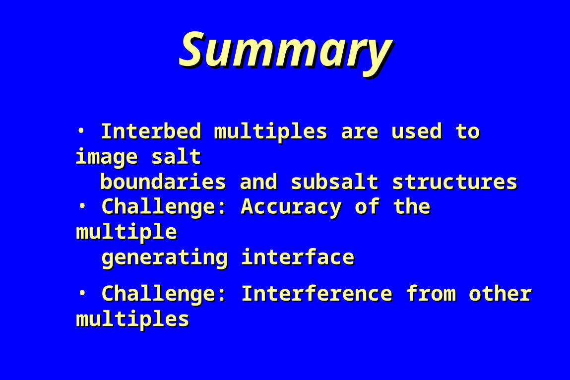
• Interbed multiples are used to image saltInterbed multiples are used to image salt boundaries and subsalt structuresboundaries and subsalt structures
SummarySummary
• Challenge: Accuracy of the multipleChallenge: Accuracy of the multiple generating interface generating interface
• Challenge: Interference from other multiplesChallenge: Interference from other multiples
OutlineOutline• OverviewOverview• Surface Multiple Migration Surface Multiple Migration • Interbed Multiple MigrationInterbed Multiple Migration• Multiple Attenuation inMultiple Attenuation in Multiple ImagingMultiple Imaging• ConclusionsConclusions

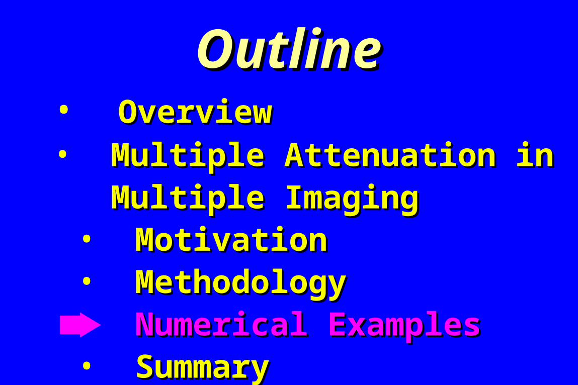
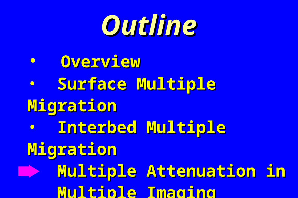
OutlineOutline• OverviewOverview• Multiple Attenuation inMultiple Attenuation in Multiple ImagingMultiple Imaging
• Motivation Motivation • Methodology Methodology • Numerical ExamplesNumerical Examples• SummarySummary

A major problem with multiple imaging:
high-order high-order multiplemultipleIncorrectly positioned as Incorrectly positioned as
low-order multiplelow-order multiple
interference from high-order multiple interference from high-order multiple

OutlineOutline• OverviewOverview• Multiple Attenuation inMultiple Attenuation in Multiple ImagingMultiple Imaging
• Motivation Motivation • Methodology Methodology • Numerical ExamplesNumerical Examples• SummarySummary

Step1: Prediction
second-order second-order multiplemultiple
SS
g’g’ gg
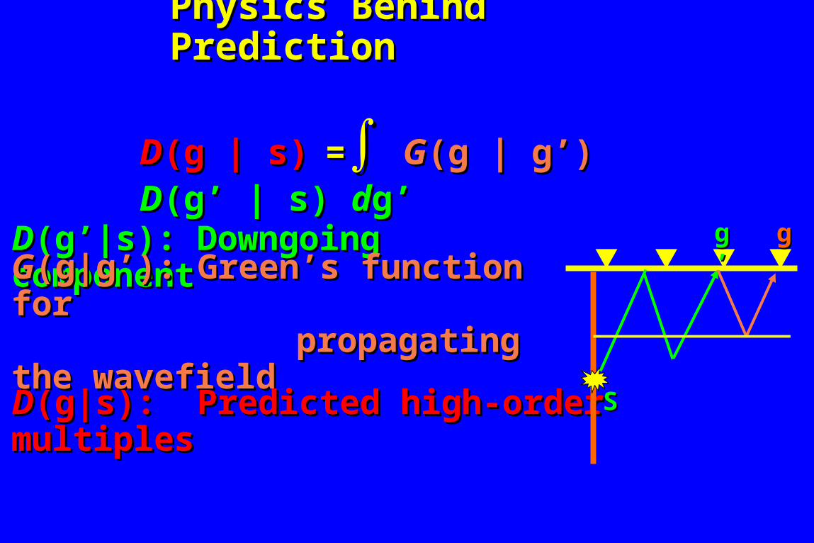
Physics Behind PredictionPhysics Behind Prediction
DD(g | s)(g | s) ==∫∫ GG(g | g’)(g | g’) DD(g’ | s)(g’ | s) ddg’g’
DD(g’|s):(g’|s): Downgoing componentDowngoing component
GG(g|g’):(g|g’): Green’s function for Green’s function for propagating the wavefield propagating the wavefield
DD(g|s):(g|s): Predicted high-order multiplesPredicted high-order multiplesSS
g’g’ gg
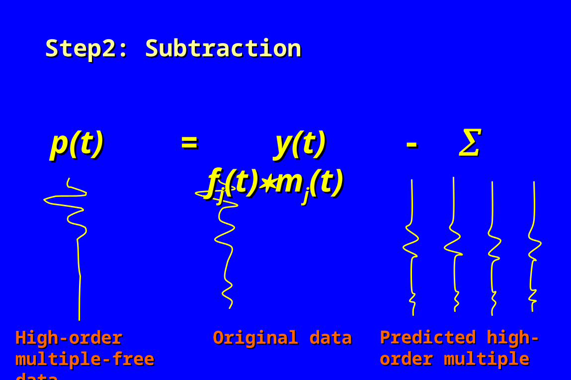
p(t)p(t) = = y(t)y(t) - - ffjj(t)(t)mmjj(t)(t)
Step2: SubtractionStep2: Subtraction
Predicted high-order Predicted high-order multiplemultiple
Original dataOriginal dataHigh-order multiple-High-order multiple-free datafree data
OutlineOutline• OverviewOverview• Multiple Attenuation inMultiple Attenuation in Multiple ImagingMultiple Imaging
• Motivation Motivation • Methodology Methodology • Numerical ExamplesNumerical Examples• SummarySummary

Numerical ExamplesNumerical Examples
• Synthetic Data TestSynthetic Data Test
• Field Data TestField Data Test

Density ModelDensity Model
00 14,00014,000X (m)X (m)
00
6,0006,000
Dep
th (
m)
Dep
th (
m)
20 receivers20 receivers6.25m spacing6.25m spacing
276 shots, 50m spacing276 shots, 50m spacing

CRG1: Different Order MultiplesCRG1: Different Order Multiples
direct wavedirect wave11stst order order
22ndnd order order
33rdrd order order

2.52.500 14,00014,000X (m)X (m)
0.40.4
Tim
e (s
ec)
Tim
e (s
ec)
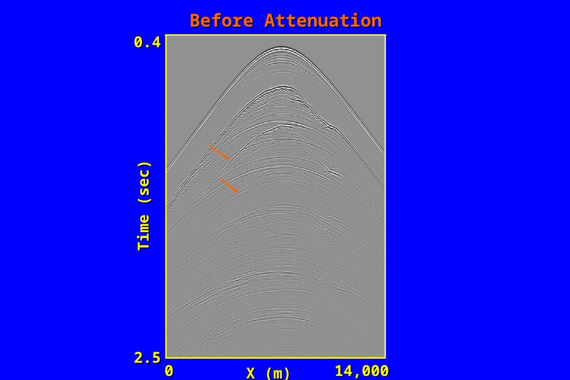
Before AttenuationBefore Attenuation
2.52.500 14,00014,000X (m)X (m)
0.40.4
Tim
e (s
ec)
Tim
e (s
ec)
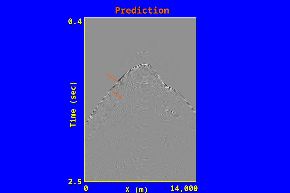
PredictionPrediction

2.52.500 14,00014,000X (m)X (m)
0.40.4
Tim
e (s
ec)
Tim
e (s
ec)
After AttenuationAfter Attenuation
2.52.500 14,00014,000X (m)X (m)
0.40.4
Tim
e (s
ec)
Tim
e (s
ec)
Before AttenuationBefore Attenuation
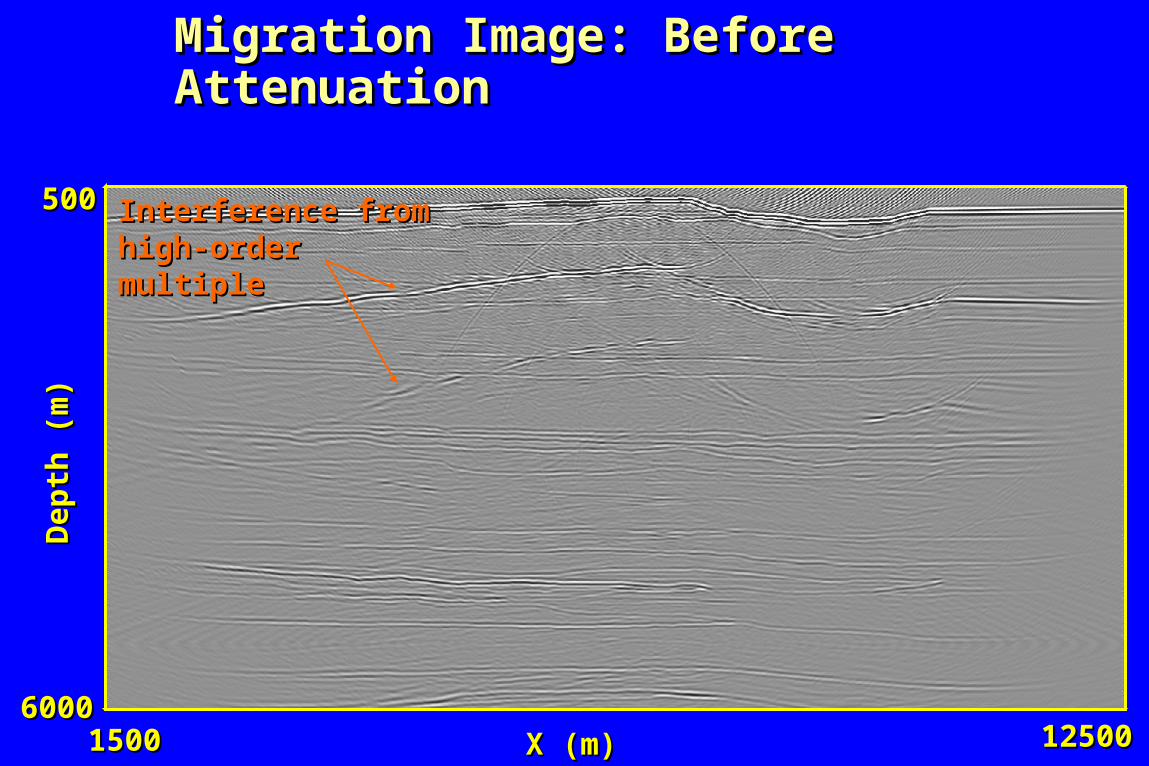
Migration Image: Before AttenuationMigration Image: Before Attenuation
500500
Dep
th (
m)
Dep
th (
m)
6000600015001500 1250012500X (m)X (m)
Interference from high-Interference from high-order multipleorder multiple
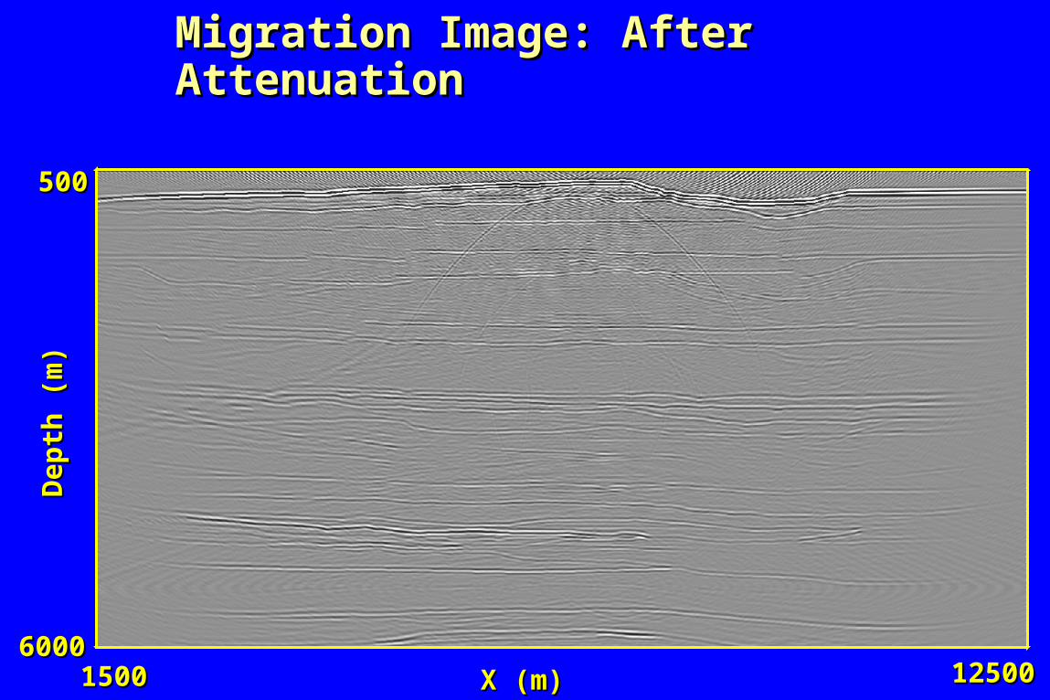
Migration Image: After AttenuationMigration Image: After Attenuation
500500
Dep
th (
m)
Dep
th (
m)
6000600015001500 1250012500X (m)X (m)
Numerical ExamplesNumerical Examples
• Synthetic Data TestSynthetic Data Test
• Field Data TestField Data Test

Velocity Model
00 6000060000X (ft)X (ft)
Dep
th (ft)
Dep
th (ft)
00
4300043000
V (ft/s)V (ft/s)49104910
1430014300
652 shots652 shots
12 receivers12 receivers

Different Order MultiplesDifferent Order Multiples
direct direct wavewave
11stst order order
22ndnd order order
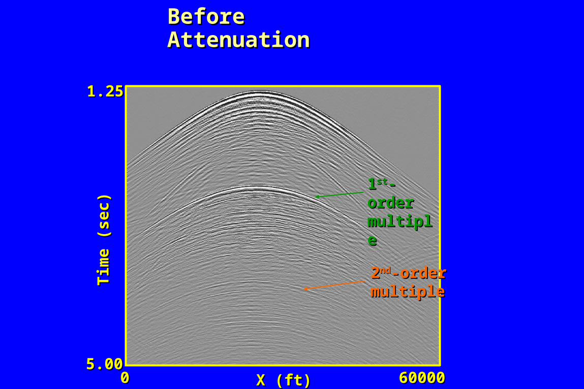
Before AttenuationBefore Attenuation
5.005.00
1.251.25T
ime
(sec
)T
ime
(sec
)
00 6000060000X (ft)X (ft)
22ndnd-order -order multiplemultiple
11stst-order -order multiplemultiple
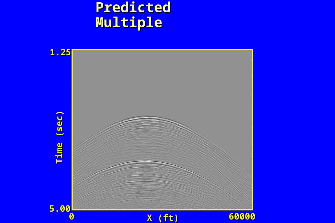
Predicted MultiplePredicted Multiple
5.005.00
1.251.25T
ime
(sec
)T
ime
(sec
)
00 6000060000X (ft)X (ft)

After AttenuationAfter Attenuation
5.005.00
1.251.25T
ime
(sec
)T
ime
(sec
)
00 6000060000X (ft)X (ft)

Before AttenuationBefore Attenuation
5.005.00
1.251.25T
ime
(sec
)T
ime
(sec
)
00 6000060000X (ft)X (ft)
22ndnd-order -order multiplemultiple
11stst-order -order multiplemultiple

Multiple Migration Image: Before AttenuationMultiple Migration Image: Before Attenuation
1010
2626
De
pth
(kft)
De
pth
(kft)
1616 3232X (kft)X (kft)
interference from high-interference from high-order multipleorder multiple

1010
2626
De
pth
(kft)
De
pth
(kft)
1616 3232X (kft)X (kft)
Multiple Migration Image: After Attenuation

Multiple Migration Images: ComparisonMultiple Migration Images: Comparison
1010
2626
De
pth
(kft)
De
pth
(kft)
1616 3232X (kft)X (kft)

OutlineOutline• OverviewOverview• Multiple Attenuation inMultiple Attenuation in Multiple ImagingMultiple Imaging
• Motivation Motivation • Methodology Methodology • Numerical ExamplesNumerical Examples• SummarySummary
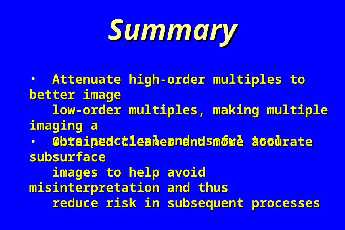
• Attenuate high-order multiples to better imageAttenuate high-order multiples to better image low-order multiples, making multiple imaging alow-order multiples, making multiple imaging a more practical and useful toolmore practical and useful tool
SummarySummary
• Obtained cleaner and more accurate subsurface Obtained cleaner and more accurate subsurface images to help avoid misinterpretation and thusimages to help avoid misinterpretation and thus reduce risk in subsequent processesreduce risk in subsequent processes
OutlineOutline• OverviewOverview• Surface Multiple Migration Surface Multiple Migration • Interbed Multiple MigrationInterbed Multiple Migration• Multiple Attenuation inMultiple Attenuation in Multiple ImagingMultiple Imaging• ConclusionsConclusions
• As shown in the numerical examples, As shown in the numerical examples, surface multiple imaging and interbedsurface multiple imaging and interbed multiple imaging can be important imagingmultiple imaging can be important imaging methods methods
ConclusionsConclusions
• The multiple attenuation process is effective in mitigating the interference in multiple imaging
• Apply data-based multiple prediction method in multiple filtering
Future WorkFuture Work
• Attenuate surface multiples prior to imaging interbed multiples
• Apply interbed multiple imaging to more field data sets

• My supervisory committee: Ronanld L. Bruhn,My supervisory committee: Ronanld L. Bruhn, Brian E. Hornby, Richard D. Jarrard, and Brian E. Hornby, Richard D. Jarrard, and Robert B. Smith
AcknowledgementsAcknowledgements
• My wife Weining and my daughter Julia
• My advisor: Gerard T. Schuster
• My UTAM colleagues and my other friends
