middleware services for structural health …
TRANSCRIPT

MIDDLEWARE SERVICES FOR STRUCTURAL HEALTH MONITORING USING SMART SENSORS
T. Nagayama,1 B. F. Spencer, Jr.,2 K. A. Mechitov,3
and G. A. Agha3
1)Department of Civil Engineering, University of Tokyo7-3-1, Hongo, Bunkyo-ku, Tokyo 113-8656, Japan
2)Department of Civil Engineering, University of Illinois at Urbana-Champaign205 N. Mathews Ave. Urbana, Illinois 61801, USA
3)Department of Computer Science, University of Illinois at Urbana-Champaign201 N. Goodwin Ave. Urbana, Illinois 61801, USA
ABSTRACT: Smart sensors densely distributed over structures can use their compu-tational and wireless communication capabilities to provide rich information forstructural health monitoring (SHM). Though smart sensor technology has seen sub-stantial advances during recent years, implementation of smart sensors on full-scalestructures has been limited. While users often postulate that wired sensing systemscan be simply replaced by wireless systems, off-the-shelf wireless systems areunlikely to provide the data users expect. Sensor component characteristics limit thequality of data collected; data from smart sensors may be inadequate due to packetloss during communication, time synchronization errors, and slow communicationspeeds. This paper addresses these issues common to smart sensor applications forstructural health monitoring by developing corresponding middleware services, i.e.,reliable communication, synchronized sensing, and model-based data aggregation.These middleware services are implemented on the Imote2 smart sensor platform, andtheir efficacy demonstrated experimentally.
1. INTRODUCTION
Dense arrays of smart sensors have the potential to improve Structural Health Monitoring (SHM)dramatically using onboard computational and wireless communication capabilities. Thesesensors provide rich information sources, which SHM algorithms can utilize to detect, locate, andassess structural damage produced by severe loading events and by progressive environmentaldeterioration. Information from densely instrumented structures is expected to result in the deeperinsight into the physical state of a structural system.
Though smart sensors have seen several demonstrative applications (Lynch and Loh 2006, Kim etal 2007), detailed validation of the data from the smart sensor networks and subsequent use fordamage detection has been limited. Measured signals are oftentimes lost during wirelesscommunication or are not synchronized with each other, limiting subsequent analyses. Theamount of data to be collected is extremely large, prohibiting spatially dense measurements and/

or the frequency of operation (Nagayama et al. 2007a). The lack of these functionalities hasprevented SHM application users from analyzing structures in detail based on smart sensormeasurement data.
This paper addresses these issues by developing corresponding middleware services that arecommon to many SHM applications. Among the middleware services are reliablecommunication, synchronized sensing, and data aggregation. These middleware services aredeveloped employing a smart sensor platform, the Imote2, which is designed for data-intensiveapplications such as SHM applications. The middleware services are then implemented on theImote2 running TinyOS. The idea behind these services are generally applicable to other smartsensor platforms, and the middleware service can be ported to platforms which have similarhardware characteristics, e.g. RAM size, as the Imote2. The implemented middleware services areevaluated and validated experimentally.
2. BACKGROUND
2.1 Reliable data transfer
RF communication is not as reliable as wired communication, due to packet loss. The mostcommon cause for packet loss results from the fact that as distance between nodes increases, thesignal-to-noise ratio drops, causing bit errors in the transmitted packet. When the receiver detectsa bit error, it drops the entire packet. Interference between multiple simultaneously transmittingnodes, called a collision, can likewise result in the loss of one or both packets. Thesecommunication failures may take place for both packets carrying commands to sensor nodes andpackets carrying measured data. If packets carrying commands are lost, destination nodes fail toperform certain tasks. When smart sensors are designed to perform complex sets of tasks,collaborating with other sensors nodes, command packet loss may cause sensor nodes to behaveunexpectedly, possibly leading to network failure. If packets carrying measurement data are lost,destination nodes cannot fully reconstruct the sender's data. SHM applications employing smartsensors must address this packet loss problem. Retransmission- and acknowledgment-basedapproaches are candidates to reduce the packet loss rate during wireless communication.Thesetwo approaches are first explained briefly.
retransmission without acknowledgment can statistically improve the reliability ofcommunication. If the packet loss rate is expected to be approximately constant over time,retransmission can virtually eliminate data loss; the number of repetitions can be dynamicallyadjusted based on measured packet loss rates. When the packet loss rate is high, the number ofrepetitions is increased. Such protocols, however, cannot guarantee communication success ratedeterministically. In smart sensor networks, burst packet loss may take place, which underminesthe effectiveness of this approach. Interference from other nearby RF transmission devicesoperating in the same frequency range, for example, may cause a large number of packets to bedropped. If the packet loss rate is high during all the successive retransmissions, the loss of manypackets is unavoidable.
Acknowledgment-based approaches can potentially guarantee reliable communication betweennodes, by continuing packet retransmission until acknowledgment is received. However, a poorly-

designed communication protocol involving acknowledgment messages can be notablyinefficient. Many acknowledgment messages may be required, waiting times may be long, and thesame packets may need to be sent many times. Furthermore, RF components on many smartsensor platforms including the Imote2 are in either a listening mode or transmission mode,making the need for frequent switch between the two modes unwelcome. During transmission,the Imote2 cannot receive packets. Nonetheless, transmission and reception are deeplyinterwoven in many acknowledgement-based approaches. Interwoven transmission and receptionof acknowledgement-based approaches may result in slow data transfer.
Instead of acknowledging each packet, the reliable communication protocol developed byMechitov et al. (2004) sends a set of packets and then waits for acknowledgment. If the receiverdoes not receive acknowledgment, the same set of packets is sent again. Upon reception ofacknowledgment, the sender moves on to the next set of packets. The size of a set of packetsneeds to be optimized. A small size of packet set necessitates a larger number ofacknowledgement packets; a large size of packet set, on the other hand, results in retransmittinglarge numbers of packets even when only one packet is lost. Therefore, the number ofacknowledgement packets cannot be drastically reduced.
2.2 Synchronized sensing
The lack of a global clock in smart sensor network is problematic for SHM applications. If modalanalysis is conducted without accurate time synchronization, the identified mode shape phase willbe inaccurate, possibly falsely indicating structural damage. Large synchronization errors makeaccurate estimation of cross spectral densities and transfer functions almost impossible.
Time synchronization for smart sensor networks has been widely investigated. By communicatingwith surrounding nodes, smart sensors can assess relative differences among their local clocks.Reference Broadcast Synchronization (RBS; Elson et al., 2002), Flooding Time SynchronizationProtocol (FTSP; Maroti et al., 2004) and Timing-sync Protocol for Sensor Networks (TPSN;Ganeriwal et al., 2003) are among the well-known synchronization methods. Mica2 motesemploying TPSN are reported to synchronize with each other to an accuracy of 50 µsec. Mechitovet al. (2004) implemented FTSP on Mica2 motes as a part of wireless data acquisition system forSHM. This system can maintain better than 1ms synchronization accuracy for minutes. Clock ratedifference(i.e., drift) from node to node increases time synchronization error over time. Whenclock drift is significant, synchronization is applied periodically before the error becomes toolarge.Thus, fine synchronization among sensor nodes has been shown achievable.
However, measured signals may not be synchronized with each other, even when clocks areprecisely synchronized. Sampling timing is not necessarily controlled precisely based on theseclocks. Whereas time synchronization protocols have been intensively studied, synchronizedsensing needs further investigation.
2.3 Data aggregation
The amount of data typically collected by SHM applications employing wired sensors normallyexceeds practical communication capabilities of smart sensor networks. In such approaches, dataneeds to be acquired at an appropriate sampling rate for a sufficient period of time at various

locations and stored at a central location. Central collection of vibration measurement data isreported to take more than ten hours (Kim et al. 2007). One approach to overcome this problemhas been to use an independent data processing strategy (i.e., without internode communication).This approach, however, cannot fully exploit information available in the sensor network (e.g.,much of spatial information is neglected). Data aggregation is an important issue to be addressedbefore an SHM system employing smart sensors can be realized.
Distribution of data processing and coordination among smart sensors play a central role inaddressing many smart sensor implementation issues, including data aggregation. Dataprocessing is application dependent. Application specific knowledge can be incorporated intodata aggregation strategies to efficiently collect information from smart sensor network.
2.4 Intel Imote2 smart sensor platform
The Imote2 is a new smart sensor platform developed for data-intensive applications (Crossbow,Inc., 2008). The main board of the Imote2 incorporates a low-power Xscale processor, thePXA271, and an 802.15.4 radio, ChipCon 2420. The processor speed may be scaled based on theapplication demands, thereby improving its power efficiency. One of the important characteristicsof the Imote2, which separates it from other commercially available wireless sensing nodes, is thememory size. The Imote2 has 256 KB of integrated SRAM, 32 MB of external SDRAM, and 32MB of Strataflash memory, which is particularly important for the large amount of data requiredfor dynamic monitoring of structures and associated data processing. The computational powerand storage capacity make the Imote2 stand unequaled among commercially available smartsensors. Intel has created a basic sensor board to interface with the Imote2. This basic sensorboard can measure 3-axes of acceleration, light, temperature, and relative humidity. All of thesensors on this board are digital, thus no analog to digital converter (ADC) is required. The 3-axisdigital accelerometer (LIS3L02DQ; STMicroelectronics, 2008) has a ±2g measurement range anda resolution of 12-bits or 0.97 mg. The Imote2 with the basic sensor board are employed in thispaper as the smart sensor platform.
3. RELIABLE COMMUNICATION
While reliable command packet transfer is clearly a significant help in developing SHM systemsrequiring complex, internode, data processing, the need for reliable data transfer requires furtherconsideration. Nagayama et al. (2007a) theoretically derived expressions for the effect of data losson power spectral density estimates and showed that data loss degrades measurement signalssimilar to that of observation noise. When packet loss is not negligibly small, data needs to bereliable transferred.
To estimate the packet loss rate in smart sensor communication and assess the need for reliablecommunication middleware services, experiments are first conducted. Then reliablecommunication protocols are proposed to transfer a large amount of data as well, as protocols tosend a single packet.

3.1 Packet loss estimation in RF communication
First, packet loss rate is experimentally estimated. A node sends a large number of packets to thereceiver nodes and packets received by the receivers are counted; this procedure is repeatedseveral times to estimate the packet loss rate. Eight Imote2s, one programming board, and a PCwere configured to perform this experiment. One of the Imote2s is programmed as the basestation. Another Imote2 works as the sender. The other six Imote2s are configured to be receivers.A java program running on the PC reads parameters from an input file and sends commands to thebase station node. The base station receives information about the number of receivers, node IDsof the sender and receivers, the number of packets to be sent, and the number of repetitions. Thebase station forwards this information to the sender. On reception, the sender starts broadcastingpackets. In this experiment, 100 packets are broadcast. After the sender completes transmission ofthe 100 packets, the sender tells the receiver that transmission is complete and queries eachreceiver regarding how many packets were received. This procedure is repeated 10 times.
This experiment is conducted on the lawn in front of Newmark Civil Engineering Laboratory atthe University of Illinois at Urbana-Champaign. The sender and receiver nodes are held at theheight of about 1 m. The distance between the sender and the receiver is 3.3 m. Figure 1summarizes the results. While many rounds of data transfer were achieved without any lostpackets, the maximum packet loss rate reached 86 percent. In many cases, the packet loss issmaller than 20 percent. The packet loss rate does not show a clear trend among the six nodes.One node without any packet loss in one round of data transfer may suffer from severe data loss inthe subsequent round of communication. Woo et al. (2003) also reported that a large packet lossrate is expected, especially when communication distance becomes large. While a loss of only afew packets is likely to take place in communication, such a low packet loss rate cannot beguaranteed.
1 2 3 4 5 6 7 8 9 100
20
40
60
80 Node1Node2Node3Node4Node5Node6
Trial
Pack
et lo
ss ra
te (%
)
Figure 1. Packet loss rate estimation.

These levels of packet loss are much larger than those discussed in Nagayama et al.(2007a) and isnot acceptable for SHM applications. A reliable communication protocol suitable for transfer of alarge amount of data, as well as a protocol for command packets, is proposed herein.
3.2 Reliable communication protocol
Reliable communication protocols for long data records and for commands are developed in thissection. In SHM applications, most communication takes place as unicast. Nonetheless, multicastof command packets is oftentimes needed. Some SHM applications can efficiently achieve dataaggregation, taking advantage of multicast of long data records as explained later. Both unicastand multicast protocols are, therefore, supported in the proposed protocols.
3.2.1 Communication protocol for long data records
Communication protocols suitable for transfer of long data records reliably are developed basedon acknowledgement approaches. In the proposed protocols, the sender transmits all of the datapackets before acknowledgment for these packets is expected. The receiver stores all of thereceived data in a buffer. Once the receiver gets a message indicating the end of data transmission,the receiver replies to the sender, indicating which packets are missing. Then, only missingpackets are resent. In this way, the number of acknowledgments and retransmissions, as well asthe need to switch between the two modes, can be greatly reduced.
Both the unicast and multicast protocols are designed to send either 64-bit double precision data,32-bit integers, or 16-bit integers. Many ADCs on traditional data acquisition systems have aresolution less than 16 bits, supporting the need for transfer of 16-bit integer format data. SomeADCs have a resolution better than 16 bits, necessitating data transfer in 32-bit integer format.Once an acceleration record is processed, the outcome may need more precision. Onboard dataprocessing such as FFTs and SVDs is usually performed using double precision calculations.Even when the effective number of bits is smaller than 32, debugging of onboard data processinggreatly benefits from transfer of double precision data; data processing results on Imote2s can bedirectly compared with those on a PC, which are most likely in double precision format. Inclusionof 64-bit double precision data transfer is based on such needs.
The maximum data length supported by the protocols is set as 11,264 for 16-bit integer data,though this length can be adjusted by changing parameters. SHM usually involves FFTcalculations; 11,264 is 11 times 1,024;1024 is often employed as the length of the FFT. Asexplained later, the longer the maximum supported data length is, the larger the RAM needed forthe protocol is. Therefore the supported data length cannot be arbitrarily increased. 11,264 datapoints in 16-bit integer format needs about 22.5 kB of RAM while the Imote2 RAM size is 256kB. When an extremely large amount of data needs to be transferred, data can be split into smallerblocks and sent block by block.

Unicast
In the unicast protocol, the sender reliably delivers long data records to a single receiver node.Figure 2 shows a flowchart of this protocol. The sender first performs a handshake and transfersthe necessary parameters. Then all the data is sent without requesting acknowledgements. Afterthis transfer, the receiver checks for missing packets and requests retransmission. Followingretransmission, the handshake is terminated. The details of the protocol are explained in thefollowing paragraphs.
On main program’s start-up, the communication middleware service requests that the mainprogram assign a buffer space to keep data to be transferred. This buffer needs to be large enoughto hold the entire data record. The main program returns the pointer to this buffer to themiddleware service. The need for this large buffer size is a drawback of this approach. However,the buffer is allocated in the main program and only the pointer is given to the communicationprogram; with knowledge of the application, the main program can utilize this memory space forother purposes when communication is not taking place.
When the application is ready to send data, the sender sends a packet and informs the receiver ofthe necessary parameters (e.g., data length, data type, message ID, destination node ID, sourcenode ID, etc.). If the data is in integer format, a scaling factor and offset of the data are alsoconveyed to the receiver so that the receiver can reconstruct the original data. All theseparameters are packed in the 28 B payload of a packet. After this transmission, the senderperiodically checks whether an acknowledgment from the receiver has arrived. If not, this packetis sent again. Once two nodes exchange this packet and engage in a round of reliablecommunication, packets with different message IDs, destination node IDs, and source node IDs
Sender Receiver
Sends parameters• Sender sends parameters to the receiver.
(e.g. data length, scaling factor, offset, data type, message ID, etc.)
• Sender keeps sending the parameters until acknowledgement is received.
Acknowledges• Receiver saves received parameters and
returns acknowledgement.Sends data
• Sender sends the entire data set. Receives data• Receiver saves received data and keeps
track of received packets.Tells the end of data transmission• Sender notifies the receiver repeatedly until
acknowledgement is received that all the data is sent out. Acknowledges/Requests missing packets
• Receiver acknowledges. If the receiver missed packets, requests sender resend the missing packets.
Sends missing data
Missing packets?
Receives data• Receiver saves received data and keeps
track of received packets.Completion of data transfer
• Sender tells the receiver that the data transfer is complete. Sender keeps sending packets until acknowledgement is received.
Acknowledges• Receiver acknowledges.
yes
no
Figure 2. Block diagram of the reliable unicast protocol for long data records.

are disregarded. The message ID of the sender is incremented when the sender engages in a newround of reliable communication.
For Imote2 nodes to appropriately interpret the received packet, 1 byte of the payload of everypacket is designated for packet interpretation instruction. For example, a packet from the senderwith the instruction ‘1’ is interpreted as the first packet with parameters such as data length, datatype, etc. On reception of a packet, tasks predetermined for the instruction are executed.
Also, the current state of the sender and receiver are internally maintained using a 1-byte variableon each node. For example, the sender’s current state is ‘1’ after sending the packet with theinstruction ‘1’. This state changes to ‘2’ when the sender finds that an acknowledgment for thispacket is received. The tasks to be executed in events such as packet reception and timer firing aredetermined based on the current state variable and the instruction byte of the most recentlyreceived packet.
Upon reception of a packet with the instruction of ‘1’ from the sender, the receiver checkswhether it is ready to receive data. Unless this node has already executed the handshake withanother node (i.e., agreed to receive data from another node or send data to another node), thisnode replies to the sender with an acknowledgment packet. The two nodes are then ready totransfer data.
When the sender notices that the acknowledgment has arrived, the periodical check foracknowledgment packets stops and the entire data record is sent to the receiver. One packetcontains either three double precision data points, six 32-bit integers, or twelve 16-bit integers.Each packet also contains a 2-byte node ID for the sender and a 2-byte packet ID, which thereceiver uses to sort received packets and reconstruct the original data in the buffer. To keep trackof received packets, the receiver maintains a bitmap of received packets, which is initialized tozeroes on reception of a packet with the instruction ‘1’. One bit of the bitmap is assigned to eachdata packet, which necessitates allocation of 235B RAM space to keep track of 11264 data pointsin integer format. Upon reception of each packet, the corresponding bit is changed to one. Byexamining this bitmap, the receiver determines which packets are missing.
When the sender finishes transmitting all the data, a packet conveying the end of the datatransmission is sent to the receiver. An instruction-byte of ‘2’ for this packet is interpreted as theend of the data transmission. The sender periodically checks the response from the receiver. Ifnothing is received, this packet is sent again.
Knowing that all of the data was transmitted from the sender, the receiver checks the bitmap tokeep track of received packets. If all of the packets were received, an acknowledgment is returnedto the sender. The sender then tells the receiver that the data transfer is complete by sending apacket with the instruction-byte of ‘4’. This message is also resent until an acknowledgmentpacket is returned from the receiver. When the receiver first acknowledges the packet with theinstruction-byte of ‘4’, the receiver signals to the main program on the receiver that a set of datahas been successfully received, thus completing the receiving activity on this node. Once thesender node receives this acknowledgment, the main application on the sender is notified that thedata has been sent out successfully, thus completing the sending activity. The handshake is calledoff and the two nodes are ready to start another round of data transfer.

If the receiver notices that some packets are missing on reception of the packet with theinstruction-byte of ‘2’, the receiver responds by sending a packet with the missing packets’ IDs.The first eight missing packets’ IDs are packed in the payload of an acknowledgment packet andsent to the sender. The sender packs these missing packets and sends them to the receiver. At theend of transmission, the packet with the instruction-byte of ‘2’ is sent again. If there are stillmissing packets, the same procedure is repeated. If all of the data is received, an acknowledgmentis returned, and the communication activity is completed as described in the previous paragraph.
One of the difficulties with this protocol is judging when communication ends This difficulty isalso known as the Byzantine Generals Problem (Lamport et al. 1982). The sender can clearlydetermine the end of communication when the acknowledgment message with the instruction-byte of ‘4’ is received. However, the receiver cannot judge the end of communicationdeterministically. The receiver does not know whether the acknowledgment with the instruction-byte of ‘4’ reaches the sender or not. If the receiver node does not receive any packet after thetransmission of this acknowledgment packet, there are two possible situations: theacknowledgment packet reached the sender and this data transfer was successfully completed;and the acknowledgment packet did not reach the sender and the sender is periodicallytransmitting packets with the instruction-byte of ‘4’, none of which arrived at the receiver node.There is no way for the receiver node to judge between the two possibilities.
This inability to judge the end of communication may cause a serious problem. If only thereceiver calls off the handshake, then the sender will keep sending the last packet to the receiver;the receiver never replies because the receiver is already disengaged from this round of datatransfer.
This problem is alleviated by storing message and source IDs of the last several rounds of reliablecommunication and separating the last acknowledgment process from the rest of the process.When the receiver gets the packet with the instruction-byte of ‘4’ for the first time, this receivernode sends an acknowledgment back and is disengaged from this communication activity. Themessage and source IDs are stored on this node. If this receiver node later receives the samepacket, the structure storing the message and source IDs is checked. Once the receiver finds in thestructure the pair of the message and source IDs that are the same as those of the received packet,an acknowledgment is sent back to the sender. This procedure to acknowledge the end of datatransfer may take place while the receiver node is engaged in another round of data transfer,giving concerns over overwriting packet buffer. For example, consider a situation where a node isengaged in a round of data transfer and about to send a packet with the instruction-byte of ‘2’. Ifthis node receives a packet with the instruction-byte of ‘4’ requesting acknowledgment fromanother node, this node fills the packet buffer with the necessary parameters foracknowledgement (e.g., the instruction-byte of ‘4’). If the packet buffer is shared for the twoprocesses, the buffer is overwritten. To avoid such overwriting, the packet buffer space for thisacknowledgment with the instruction-byte of ‘4’ is assigned separately from the packet bufferspace for others. Even when the receiver is engaged in the next round of communication, thisprocess of acknowledgment can be done without affecting the subsequent or ongoingcommunication activities.
Multicast
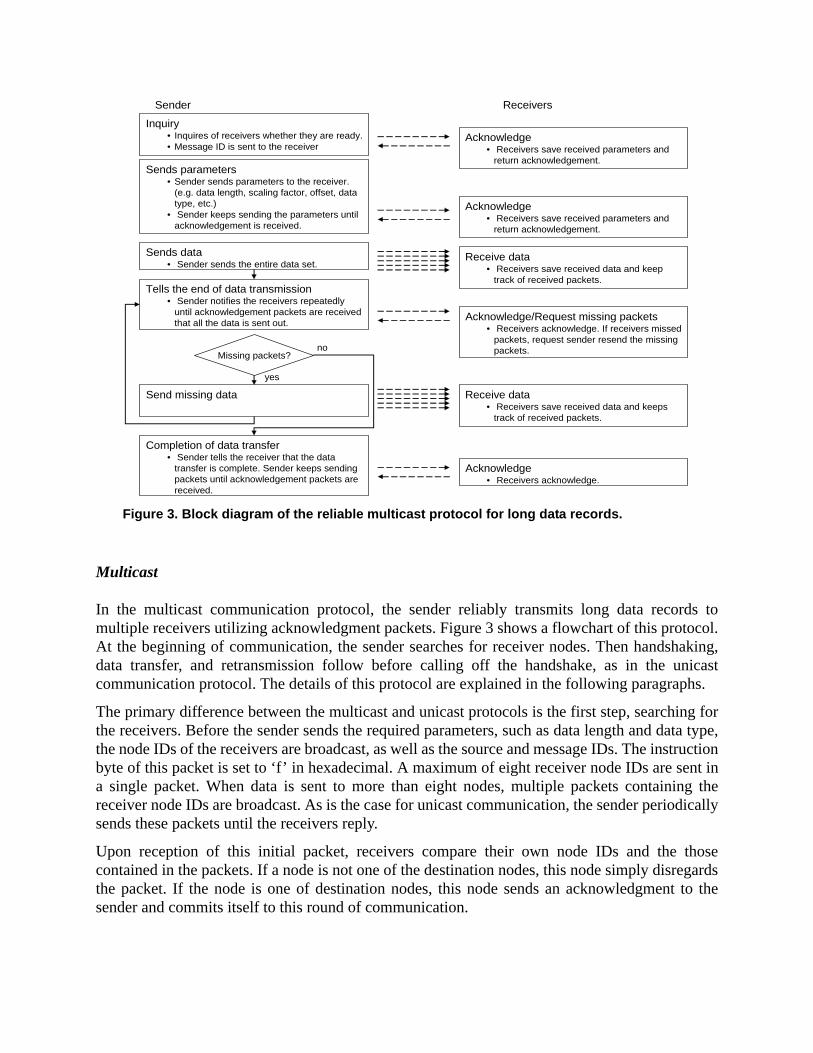
In the multicast communication protocol, the sender reliably transmits long data records tomultiple receivers utilizing acknowledgment packets. Figure 3 shows a flowchart of this protocol.At the beginning of communication, the sender searches for receiver nodes. Then handshaking,data transfer, and retransmission follow before calling off the handshake, as in the unicastcommunication protocol. The details of this protocol are explained in the following paragraphs.
The primary difference between the multicast and unicast protocols is the first step, searching forthe receivers. Before the sender sends the required parameters, such as data length and data type,the node IDs of the receivers are broadcast, as well as the source and message IDs. The instructionbyte of this packet is set to ‘f’ in hexadecimal. A maximum of eight receiver node IDs are sent ina single packet. When data is sent to more than eight nodes, multiple packets containing thereceiver node IDs are broadcast. As is the case for unicast communication, the sender periodicallysends these packets until the receivers reply.
Upon reception of this initial packet, receivers compare their own node IDs and the thosecontained in the packets. If a node is not one of the destination nodes, this node simply disregardsthe packet. If the node is one of destination nodes, this node sends an acknowledgment to thesender and commits itself to this round of communication.
Sender Receivers
Sends parameters• Sender sends parameters to the receiver.
(e.g. data length, scaling factor, offset, data type, etc.)
• Sender keeps sending the parameters until acknowledgement is received.
Acknowledge• Receivers save received parameters and
return acknowledgement.
Sends data• Sender sends the entire data set.
Receive data• Receivers save received data and keep
track of received packets.Tells the end of data transmission
• Sender notifies the receivers repeatedly until acknowledgement packets are received that all the data is sent out. Acknowledge/Request missing packets
• Receivers acknowledge. If receivers missed packets, request sender resend the missing packets.
Send missing data Receive data• Receivers save received data and keeps
track of received packets.
Completion of data transfer• Sender tells the receiver that the data
transfer is complete. Sender keeps sending packets until acknowledgement packets are received.
Acknowledge• Receivers acknowledge.
yes
noMissing packets?
Inquiry• Inquires of receivers whether they are ready.• Message ID is sent to the receiver
Acknowledge• Receivers save received parameters and
return acknowledgement.
Figure 3. Block diagram of the reliable multicast protocol for long data records.

Note that if multiple receivers reply to the sender at the same time, packet collision may takeplace; timing for replies to the sender needs to be scheduled appropriately. The order of node IDsin the packets with the instruction-byte of ‘f’ is used to schedule the timing for replies. Forexample, the node corresponding to the eighth node ID in the packet with the ‘f’ instruction-bytewaits 7 x seconds before the acknowledgment is sent back to the sender; is unit waiting time.The order of reply and are stored on each receiver; all of the following acknowledgmentmessages in this multicast protocol use this scheduling. Optimization of the waiting interval, ,may result in faster communication; such optimization has not been pursued yet.
Once the sender receives an acknowledgment from all of the receivers, the parameters such asdata length, data type, scaling factor, and offset are broadcast. Although the broadcasttransmission reaches all of the nodes in the neighborhood, only the engaged nodes process thereceived packet. The source ID, the destination ID (i.e., node ID of ‘ffff’ in hexadecimal, whichcorresponds to broadcast address in TinyOS), and the message ID are used on receivers todistinguish packets to be processed from other packets.
Another difference between unicast and multicast is that the sender needs to check theacknowledgment messages from all of the receivers. The sender keeps track of acknowledgmentsfrom the receivers using a bitmap. One bit of the bitmap corresponds to one receiver. Before thesender transmits a packet needing acknowledgement from the receivers, this bitmap is initializedto zeroes. Upon reception of an acknowledgment from a receiver, the bit corresponding to thisreceiver is changed to one. While the size of this bitmap currently is set so that up to 32 nodes canbe receivers, parameters can be easily adjusted to accommodate a larger number of receivers atthe expense of the memory required for storing the bitmap.
Another point to consider is the way that requests for retransmission are handled. After sendingthe end-of-transmission notice packet to the receivers, the sender waits for a reply from therespective receivers. Within the assigned time slot, each receiver sends back an acknowledgmentpacket containing missing packet IDs. After the time assigned for all of the nodes to reply haspassed, the sender broadcasts the requested packets. At the end of broadcast of these requestedpackets, a packet with the instruction-byte of ‘2’ is sent, asking for packets still missing.
The end of one round of communication is achieved in a similar manner to that implemented forunicast reliable communication. In addition to the message and source IDs, this multicast protocolrequires the receiver nodes store the waiting time before replying with acknowledgment.
3.2.2 Communication protocol for commands
Communication protocols suitable to transfer a single packet reliably are also needed. SHMapplications involve sending and receiving many commands, each of which fits in one packet.These commands need to be delivered reliably. If a packet containing a command to start sensingis lost, the destination node does not start sensing. The sender node cannot deteministically judgeif a certain command was delivered and executed at the receiver nodes. The current states of smartsensor nodes are hard to estimate without reliable communication. Ensuring the performance ofSHM systems without reliable command delivery is extremely complex if not impossible. Thereliable communication protocol developed for long data records is, however, not efficient for
β ββ
β

single packet transfer. Unicast and multicast reliable communication protocols suitable for single-packet messages are developed.
This protocol is again similar to the ARQ protocol. Because only one packet is sent, anacknowledgment is returned to the sender for each packet. The protocol is designed to sendcommands and parameters in 8- and 16-bit integers. The payload of one packet can hold nine 16-bit integers and one 8-bit integer in addition to communication parameters such as source andmessage IDs.
Unicast
The sender transmits a packet, including the destination ID, source ID, message ID, command,and other parameters. Until this packet is acknowledged, the sender continues to transmit thispacket. The receiver extracts information from the packet and sends an acknowledgment back tothe sender (see Figures 4).
The end of one round of communication is implemented in a manner similar to that for thereliable unicast protocol for long data records. The source and message IDs for the last severalrounds of communication are stored so that acknowledgment can be sent even after the receiver isdisengaged from this round of communication.
Multicast
The multicast protocol is implemented in a similar manner to the unicast protocol. As is the casefor protocols for long data records, the primary difference is the first step, searching for thereceivers. The sender first transmits a packet including the receivers’ node IDs, as was the casefor the multicast communication protocol for long data records. Once all of the receivers returnacknowledgment packets to the sender, the sender transmits a packet containing a command andassociated parameters. The receivers also acknowledge this packet. To judge the end ofcommunication, the receiver keeps the source ID, message ID, and waiting time of the last severalrounds of communication (see Figures 5).
Sends a packet• Sender keeps sending a packet until
acknowledgement is received.
Acknowledges• Receiver saves received command/
parameters and returns acknowledgement.
ReceiverSender
Figure 4. Block diagram of the reliable unicast protocol for commands.
Sender Receivers
Sends a packet• Sender keeps sending the packet until
acknowledgement is received.Acknowledge
• Receivers save received command/ parameters and return acknowledgement
Inquiry• Inquires of receivers whether they are ready
Acknowledge• Receivers save received parameters and
return acknowledgement
Figure 5. Block diagram of the reliable multicast protocol for commands.

4. SYNCHRONIZED SENSING
Measured signals from a smart sensor network with the intrinsic local time differences need to besynchronized. If not appropriately addressed, time synchronization errors can cause inaccuracy inSHM applications, particularly in the mode shape phases (Nagayama 2007). Timesynchronization accuracy realized on the Imote2 is first estimated and evaluated for the SHMapplications. Time synchronization among smart sensors does not necessarily offer synchronizedmeasurement signals. Even when the clocks of sensor nodes are perfectly synchronized with eachother, measured signals may not be accurately time-aligned. Issues critical to synchronizedsensing are then investigated and synchronized sensing is realized utilizing a resampling approach(Nagayama 2007; Nagayama et al. 2006a, 2007a, & 2007b; Spencer and Nagayama, 2006).
4.1 Estimation of time synchronization error
The accuracy of the Flooding Time Synchronization Protocol (FTSP; Maroti et al., 2004)implementation on the Imote2 is evaluated. This protocol is first reviewed briefly, and then theaccuracy is examined in terms of synchronization errors and clock drift.
FTSP utilizes time stamps on the sender and receivers. A beacon node broadcasts a packet to theother nodes. At the end of the packet, a time stamp, , is appended just before transmission.Upon reception of the packet, the receivers stamp the time, , using their own local clocks.The delivery time, , between these two events includes interrupt handling time, encodingtime, and decoding time. is usually not small enough to be ignored; the variance of
over time is usually small. can be estimated in several ways. An oscilloscopeconnected to both nodes and on-board clocks can keep track of the communication time stamp. Inthis study, is first assumed to be zero and then adjusted so that Imote2s placed on thesame shake table give synchronized acceleration data. If these nodes are synchronized, the phasesof the transfer functions among Imote2 signals should be constant over wide frequency range.
is determined to give a constant phase of zero. Using this value, the offset between thelocal clock on the receiver and the reference clock on the sender is determined as
. This offset is subtracted from the local time when global time stampsare requested afterward.
To evaluate time synchronization error, a group of nine Imote2s are programmed as follows. Thebeacon node transmits a beacon signal every 4 seconds. The other eight nodes estimate the globaltime using the beacon packet. Time synchronization is thus performed. Two seconds after thebeacon signal, the beacon node sends the second packet, requesting replies. The receivers get timestamps on reception of this packet and convert them to a global time stamp using the offsetestimated 2 seconds before. These time stamps are subject to two error sources: First, timesynchronization error, and second, delay in time stamping upon reception of the second packet.The receivers take turns to report back these time stamps. This procedure is repeated more than300 times. These time stamps from the eight nodes are compared. Figure 6 shows the difference inthe reported global time stamps using one of the eight nodes as a reference. The timesynchronization error seems to be less than 10 µs for most of the time. Scattered peaks mayindicate large synchronization error. Note that the time synchronization error is one of the two
tsendtreceive
tdeliverytdelivery
tdelivery tdelivery
tdelivery
tdelivery
treceive tsend– tdelivery–

above-mentioned factors explaining the error in the time stamps. This figure indicates that anupper-bound estimate of time synchronization error is 80 µs.
The time synchronization error estimated above is considered small for SHM applications. Thedelay of 10 µsec corresponds to a 0.072-degree phase error for a mode at 20 Hz. Even at 100 Hz,the corresponding phase error is only 0.36 degree.
The same approach is utilized to estimate clock drift. Upon reception of the second packet, whichrequests replies, the receivers return to the sender their offsets to estimate the global time, insteadof global time stamps. If clocks on nodes are ticking at exactly the same rate, the offsets should beconstant. This experiment, however, did not show constant offsets. Figure 7 shows the offsets ofeight receiver nodes. This figure shows that the drift rate is quite constant in time. The maximumclock drift rate among this set of Imote2 nodes is estimated to be around 50 µs per second. Notethat this estimate from the eight nodes is not the upper limit of clock drift because of the small
50 100 150 200 250 300
-80
-40
0
40
80
Repetition
Tim
e (µ
sec)
Figure 6. Time synchronization error estimation.
0 40 80 120 160-4000
0
4000
8000
Time (sec)
Drif
t(µs
ec)
Figure 7. Drift estimation.

sample size. This drift is small but not negligible if long measurement records are taken. Forexample, after a 200 second measurement, the time synchronization error may become as large as10 ms.
One solution to address this clock drift problem is frequent time synchronization. Timesynchronization could be performed often to prevent the synchronization error fromaccumulating. However, frequent time synchronization is not always feasible. When other tasksare running (e.g., sensing), time synchronization may not perform well. Time synchronizationrequires precise time stamping while sensing requires precise timing and needs higher priority inexecution. Scheduling more than one high priority tasks is challenging, especially for anoperating system such as TinyOS, which does not support strict real-time control. If the timesynchronization interval is shorter than the sensing duration, another solution needs to be soughtto avoid interference between time synchronization and sensing tasks.
The slopes of the lines in Figure 7 are nearly constant and provide an estimate of the clock ratedifference. If time synchronization offset values can be observed for a certain amount of time, theslope can be estimated using a least-squares approach. The difference in clock rate is estimatedand taken into account in the subsequent data processing as described in Section 4.2.
4.2 Issues toward synchronized sensing
Accurate synchronization of local clocks on Imote2s does not guarantee that measured signals aresynchronized. Measurement timing cannot necessarily be controlled based on the global time. Tobetter understand this situation, the sensing process on the Imote2 is first described.
The sensing application program on the Imote2 calls sensor driver commands to perform sensingand obtains measurement data in the following way. A sensing application posts a task to preparefor sensing. Parameters such as the sampling frequency and the total number of data points arepassed to the driver. Once the sensor driver becomes ready, sensing starts. The sensing taskcontinues running until a predefined amount of data is acquired. During this sensing, the acquireddata points are first stored in a buffer. Every time the buffer is filled, the driver passes the data tothe sensing application. This block buffered data is supplied with a local time stamp marked whenthe last data point of the block is acquired. The clock used for the time stamp runs at 3.25 MHz. Iftime synchronization is performed prior to sensing, the offset between the global and local timescan be utilized to convert the local time stamp to a global time stamp when needed. The data andtime stamps passed are copied to arrays in the sensing application, and the buffer is returned to thedriver to be used for the next block of data.
Building synchronized sensing on this sampling process is challenging. The difficulties areexplained next.
1. Uncertainty in start-up time
Starting sensing tasks at all of the Imote2 nodes in a synchronous manner is problematic. Evenwhen the commands to start sensing are queued at exactly the same moment, the execution timingof the commands is different on each node. Thus, measured signals are not necessarilysynchronized to each other.

TinyOS has only two types of threads of execution: tasks and hardware event handlers, leavingusers little control to assign priority to commands; if sensing is queued as a task, this task isexecuted after all the tasks in the front of the queue are completed. As such, the waiting timecannot be predicted. If the command is invoked in a hardware interrupt as an asynchronouscommand, this command is executed immediately unless other hardware interrupts interfere.However, invocation of commands as a hardware interrupt from a clock firing at very highfrequency is not practical; firing the timer at a frequency corresponding to the synchronizationaccuracy, tens of microseconds, is impossible.
In addition, the warm-up time for sensing devices after the invocation of the start command is notdeterministic. Even if the commands are invoked at the same time, sensing will not startsimultaneously.
2. Difference in sampling rate among sensor nodes
The sampling frequency of the accelerometer on the available Imote2 sensor boards hasnonnegligible random error. According to the data sheet of the accelerometer, the samplingfrequency may differ from the nominal value by at most 10 percent (STMicroelectronics, 2008).Such variation was observed when 14 Imote2 sensor boards were calibrated on a shake table (seeFigure 8). Differences in the sampling frequencies among the sensor nodes result in inaccurateestimation of structural properties unless appropriate post processing is performed. If signals fromsensors with nonuniform sampling frequency are used for modal analysis, one physical mode maybe identified as several modes spread around the true natural frequency (Nagayama et al., 2006a).
3. Fluctuation in sampling frequency over time
Additionally, nonconstant sampling rate was observed with the Imote2 sensor boards, which if notaddressed, results in a seriously degraded acceleration measurement. When a block of data isavailable from the accelerometer, the Imote2 receives the digital acceleration signal and obtain thetime stamp of the last data point. By comparing differences between two consecutive time stamps,
520 540 560 580 600 6200
1
2
3
4
Sampling frequency (Hz)
Cou
nt
set value: 560 Hz
Figure 8. Sampling frequencies of 14 sensor boards.

the sampling frequency of the accelerometer is estimated. Figure 9 shows the difference betweenthe time stamps when the block size is set at 110 data points. This figure provides an indication ofthe variation in the sampling frequency. The difference in two consecutive timestamps fluctuatesby about 0.1 percent. Though imperfect time stamping on the Imote2 is a possible source of theapparent nonconstant sampling rate, the slowly fluctuating trend suggests the variable samplingfrequency as a credible cause of the phenomenon. With this fluctuation, measurement signals maysuffer from a large synchronization error and a nonconstant sampling rate.
4.3 Realization of synchronized sensing
Strict execution timing control is a possible solution for synchronized sensing. Real-timeoperating systems implemented for industrial systems with ample hardware resources can managecommand execution timing precisely. Small embedded systems without operating systems canalso be configured to manage execution timing precisely; however, implementation of real-timeoperation makes the system large and complex. Real-time control of wireless sensors in a networkis particularly challenging; the situation is exacerbated for the high sampling rates required inSHM applications. Also, even when a sensor node itself has real-time control, the peripheraldevices such as sensor chip may have execution time delay or uncertainty in timing. Instead ofpursuing real time control, synchronized sensing is realized herein using post-processing on thenon-real-time OS of the Imote2, TinyOS.
Resampling based on the global time stamps addresses the three problems: (a) uncertainty in start-up time, (b) difference in sampling rate among sensor nodes, and (c) time fluctuation in thesampling frequency. The basics of resampling and polyphase implementation of resampling arefirst reviewed. The resampling approach is then modified to achieve a sampling rate conversionby a noninteger factor. Finally, this proposed resampling method is combined with time stamps ofmeasured data to address concurrently the three issues.
0 50 100 150 200 2501.8690
1.8695
1.8700
1.8705
1.8710
1.8715x10⁵
# of data blocks
Tim
e(µ
sec)
meas urement 1meas urement 2
Figure 9. Variation in the sampling frequency over time.

Resampling
Resampling by a rational factor is performed by a combination of interpolation, filtering, anddecimation. Consider the case in which the ratio of the sampling rate before and after resamplingis expressed as an rational factor, . The signal is first upsampled by a factor of L. Then thesignal is downsampled by a factor of M. Before downsampling, a lowpass filter is applied toeliminate aliasing and unnecessary high-frequency components (see Figure 10). Using thisapproach, the signal components below the filter’s cut-off frequency are kept unchanged throughthe resampling process, though imperfect filtering such as ripples in the passband slightly distortthe signal.
During upsampling, the original signal x[n] is interpolated by -1 zeroes as in Eq. (1),
(1)
where is the upsampled signal. In the frequency domain, insertion of zeroes creates scaledmirror images of the original signal in the frequency range between the new and old Nyquistfrequencies. A discrete-time lowpass filter with a cutoff frequency, , is applied so that all ofthese images except for the one corresponding to the original signal are eliminated. To scaleproperly, the gain of the filter is set to be .
Before decimation, all of the frequency components above the new Nyquist frequency need to beeliminated. A discrete-time, lowpass filter with a cutoff frequency and gain 1 is applied.This lowpass filter can be combined with the one in the upsampling process. The cutoff frequencyof the filter is set to be the smaller value of and . The gain is .
Decimation by a factor of is then performed. Thus, the combination of upsampling, filtering,and decimation completes the resampling process.
One of the possible error sources of this resampling process is imperfect filtering. A perfect filter,which has a unity gain in the passband and a zero in the stopband, needs an infinite number offilter coefficients. With a finite number of filter coefficients, passband and stopband ripplescannot be zero. A filter design with 0.1 to 2 percent ripple is frequently used. Figure 11 showssignals before and after resampling. A signal analytically defined as a combination of sinusoidal
L M⁄
LL MM
Figure 10. The basic idea of resampling.
L
v n[ ]x n/L[ ],0,⎩
⎨⎧
=n 0 L 2L,...±,±,=
otherwise
v n[ ]
π L⁄
L
π M⁄
π L⁄ π M⁄ L
M

waves is sampled at three slightly different sampling frequencies. Two of the signals are thenresampled at the sampling frequency of the other signal. As can be seen from Figure 11, afterresampling, the three signals are almost identical. These signals are, however, not exactly thesame due to the imperfect filtering. Though this signal distortion during filtering is preferablysuppressed, this resampling process is not the only cause of such distortion. Other digital filtersand AA filters also use imperfect filters. The filter in the resampling process needs to be designedso that it does not degrade signals as compared with the other filters.
The resampling process is considered to be extremely challenging if the upsampling factor, , islarge. This issue is explained herein with examples. When a signal sampled at 100 Hz isresampled at 150 Hz, the rational factor, , is 3/2. The original signal is upsampled by a factorof 3. A lowpass filter with a cutoff frequency of can be easily designed with a reasonablenumber of filter coefficients. Note that the cutoff frequency of the filter is expressed in radiannormalized to the sampling frequency of an upsampled signal. This filter is applied to theupsampled signal, which is three times longer than the original one, and then downsampled by afactor of 2. When a signal sampled at 101 Hz is resampled at 150 Hz, on the other hand, therational factor, , is 150/101. Upsampling by a factor of 101 greatly increases the data size. Alowpass filter with a cutoff frequency of requires a large number of filter coefficients. Ifsuch a filter is applied to the upsampled signal, the upsampled signal is 101 times longer than theoriginal one. Direct implementation of such resampling on resource-limited smart sensors isintractable.
Polyphase implementation
A Finite Impulse Response (FIR) filter can be computationally much more inexpensive than anInfinite Impulse Response (IIR) filter as a filter for resampling if the polyphase implementation isemployed. The polyphase implementation leverages knowledge that upsampling involvesinserting many zeroes and that an FIR filter does not need to calculate the output at all of theupsampled data points. This implementation of resampling is explained in this section mainly inthe time domain because the extension of the method to achieve synchronized sensing is pursued
27.9 27.95 28-3
-2
-1
0
1
2
3
Time (sec)
Sig
nal v
alue
27.9 27.95 28-3
-2
-1
0
1
2
3
Time (sec)
Sig
nal v
alue
Figure 11. Signals (a) before and (b) after resampling.(a) (b)
L
L M⁄π 3⁄
L M⁄π 150⁄

using a time domain analysis. Oppenheim et al. (1999) provided a detailed description of thepolyphase implementation in the Z-domain.
Upsampling and lowpass filtering with an FIR filter can be written in the following manner:
(2)
where is the original signal, is the upsampled signal, and is the filtered signal. is a vector of the filter coefficients for the lowpass FIR filter. The length of the vector of
filter coefficients is . is, again, an interpolation factor. By combining the two relationships inEq (2) and the following,
(3)
upsampling and filtering can be written as
. (4)
where and represent the ceiling and floor functions, respectively. The number ofalgebraic operations is reduced in this equation using the knowledge that is zero at manypoints.
Downsampling by a factor of is formulated as
(5)
where is the downsampled signal. The outputs do not need to be calculated at all of the datapoints of the upsampled signal; rather, they should be calculated only at every M-th data point ofthe upsampled signal. If an IIR filter was employed, the filter would need outputs at all of the datapoints of the upsampled signal. This polyphase implementation, thus, reduces the number ofnumerical operations involved in resampling. However, implementation is still challenging if theupsampling factor, , is exceedingly large.
y n[ ] h k[ ]v n-k[ ]
k=0
N-1
∑=
v l[ ]x m[ ],
0, ⎩⎨⎧
=l = Lm, m =0, 1, 2, …±±
otherwise
x n[ ] v l[ ] y n[ ]h k[ ]
N L
Lm = n-k
y n[ ] h n-Lm[ ]x m[ ]
m= n-N+ 1 L⁄
n/L
∑=
v l[ ]
M
z j[ ] y jM[ ]=
h jM-Lm[ ]x m[ ]
m= jM-N+ 1 L⁄
jM/L
∑= j=0, 1 2 …,±,±
z j[ ]
L

Resampling with a noninteger downsampling factor
FIR filter design becomes quite difficult when sampling frequencies need to be preciselyconverted. For example, resampling of a signal from 100.01 to 150 Hz requires a lowpass filterwith a cutoff frequency of . The filter needs tens of thousands of filter coefficients.Design of such a filter is computationally challenging. Also a large number of filter coefficientsmay not fit in the available memory on smart sensors. This problem is addressed mainly byintroducing linear interpolation.
First, the resampling is generalized by introducing an initial delay, . Eq. (5) is rewritten with as follows:
(6)
where is integer. By introducing , the beginning point of the downsampled signal can befinely adjusted. If the time difference at the start of sensing is taken into account by , thesynchronization accuracy of signals is not limited by the original sampling period.
Resampling is then combined with linear interpolation to achieve the necessary accuracy. Theinteger, is replaced by a real number, , and the integer is replaced by a real number, .The upsampling rate, , must remain an integer. In this case, and are not uniquelydetermined. These values are chosen so that is not too large. A large value of requires ahigh-order lowpass filter, as is the case for the normal polyphase implementation of resampling.Using these upsampling and downsampling factors, resampling is performed. Upsampling is thesame as previously described. However, the downsampling process shown in Eq. (6) cannot bedirectly applied, due to the noninteger downsampling factor. Output data points to be calculateddo not necessarily correspond to points on the upsampled signal. Output data points often fallbetween upsampled data points. Linear interpolation is used to calculate output values as follows:
(7)
π 15000⁄
li li
z j[ ] y jM li+[ ]=
h jM+li-Lm[ ]x m[ ]
m= jM li N– 1+ +( ) L⁄
jM+li( )/L
∑= j=0, 1 2 …,±,±
li lili
M Mr li lriLa Mr La
La La
z j[ ] y pl[ ] pu pj–( )⋅ y pu[ ] pj pl–( )⋅+=
h pl Lam–[ ]x m[ ]
m= pl N– 1+( ) La⁄
pl La⁄
∑ pu pj–( )⋅=
h pu Lam–[ ]x m[ ]
m= pu N– 1+( ) La⁄
pu La⁄
∑+ pj pl–( )⋅
pj jMr lai+=
pl jMr lai+=
pu pl 1+=
In this way, resampling of an arbitrary noninteger rational factor can be achieved. When is nottoo small, linear interpolation is effective. A value of ranging from 20 to 150 is employed inalgorithmic testing and shown to give reasonable results.
Imote2 implementation using piecewise resampling of time stamped blocks of data
The proposed resampling approach is employed to address issues toward synchronized sensing.Implementation of this approach is first overviewed.
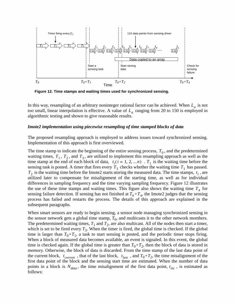
The time stamp to indicate the beginning of the entire sensing process, , and the predeterminedwaiting times, , , and , are utilized to implement this resampling approach as well as thetime stamp at the end of each block of data, . is the waiting time before thesensing task is posted. A timer that fires every checks whether the waiting time has passed.
is the waiting time before the Imote2 starts storing the measured data. The time stamps, , areutilized later to compensate for misalignment of the starting time, as well as for individualdifferences in sampling frequency and the time varying sampling frequency. Figure 12 illustratesthe use of these time stamps and waiting times. This figure also shows the waiting time forsensing failure detection. If sensing has not finished at , the Imote2 judges that the sensingprocess has failed and restarts the process. The details of this approach are explained in thesubsequent paragraphs.
When smart sensors are ready to begin sensing, a sensor node managing synchronized sensing inthe sensor network gets a global time stamp, T0, and multicasts it to the other network members.The predetermined waiting times, T1 and T2, are also multicast. All of the nodes then start a timer,which is set to be fired every T3. When the timer is fired, the global time is checked. If the globaltime is larger than T0+T1, a task to start sensing is posted, and the periodic timer stops firing.When a block of measured data becomes available, an event is signaled. In this event, the globaltime is checked again. If the global time is greater than T0+T2, then the block of data is stored inmemory. Otherwise, the block of data is discarded. From the time stamp of the last data point ofthe current block, , that of the last block, , and T0+T2, the time misalignment of thefirst data point of the block and the sensing start time are estimated. When the number of datapoints in a block is , the time misalignment of the first data point, , is estimated asfollows:
LaLa
T0T1 T2 T3
ti i 1 2 ...n, ,=( ) T1T3 T1
T2 ti
T3…
T0 T0+T1 T0+T2 T0+T4
Start asensing task
Start storingdata
Data copied to an array
t1 t2 t3 t4 t5 t6 t7 t8 tn110 110 110 110 110 110 110 110 110
110 data points from sensing driver
Check forsensingfailure
Timer firing every
Time
T3 T3 T3
T3
Figure 12. Time stamps and waiting times used for synchronized sensing.
T4T0+T4
tcurrent tlast
Ndata tini

(8)
where is later used in resampling as in Eq. (7) for the first block of data to compensatefor misalignment of the starting time (see Figure 13).
Timestamps and resampling also compensate for difference and fluctuation in the samplingfrequency (see Figure 14). The sampling frequency of the current data block, ,isestimated from and .
(9)
tini T0+T2 tlast–tcurrent tlast–
Ndata---------------------------–=
tini lai
tcurrenttlast
N
Original signal
Resampled signal
lai
The 1st block
T0+T2
T0+T2-tlasttcurrent - tlast
Figure 13. Resampling of the first block of data.
fscurrenttcurrent tlast
t last, resample
Resamplingfor the i-th block
tcurrenttlast
N tlast - t1fs
Original signal
Resampled signal
lai
x’[n]
xprev xcurrent xnext [n][n][n]
last, resample
(tcurrent - tlast)(N-1)
Figure 14. Resampling of the i-th block of data (i>1).
fscurrenttcurrent tlast–
Ndata---------------------------=

The sampling rate conversion by a factor is applied to the block of data. Thedownsampling factor is determined by
(10)
where is the sampling rate after the rate conversion. in Eq. (7) for the first block of data is. For the subsequent blocks, is determined by the time of the last resampled point of the
previous block, . Because Eq. (7) requires in blocks before or after the currentblock, data in these blocks are also utilized. To be more specific, when resampling is applied tothe current block of data, data from the block before and after the current block are used as part ofthe input signal for the resampling, , i.e.,
(11)
where , , and are data in the previous, current, and next blocks, respectively.The sampling frequency of is assumed to be same as that of . for isthen calculated as
(12)
Using these parameters, Eq. (7) is applied to each data block.
This approach can thus address uncertainty in start-up time, differences in sampling rate amongnodes, fluctuation of the frequency over time while the upsampling factor is kept moderate.This resampling-based approach, however, cannot be applied on-the-fly by the Imote2s. Theresampling is applied after all of the Imote2s have acquired signals.
While this algorithm can be implemented on Imote2s to achieve synchronized sensing, numericaloperations are nontrivial. Eq. (7) still needs a large number of multiplications, additions, etc.; thenumber of coefficients is still large, frequently greater than a thousand. One thousand filtercoefficients in double precision, for example, occupy 8 kB of memory space. These issues areaddressed by employing integer operations when applicable.
As is apparent from Eq. (7), scaling FIR filter coefficients results in filter outputs scaled by thesame factor. FIR filter coefficients are multiplied by a large constant, , so that these coefficientscan be well approximated by 16-bit integers.
(13)
These 16-bit integers representing are stored on the Imote2s instead of 64-bit doubleprecision data, saving considerable memory space. The scaled output, and in Eq.(14) are estimated only by integer operations; and are both integer type variables.
fs fscurrent⁄
Mr fscurrent L⋅ a fs⁄=
fs laitini lai
tlast,resample x m[ ]
x' n[ ]
x' n[ ]
xprev n[ ] 0 n<Ndata≤
xcurrent n-Ndata[ ] Ndata n 2Ndata<≤
xnext n-2Ndata[ ] 2Ndata n 3Ndata<≤⎩⎪⎨⎪⎧
=
xprev xcurrent xnextx' n[ ] xcurrent n[ ] lai x' n[ ]
lai tcurrent tlast–( ) Ndata 1–( ) Ndata⁄⋅ tlast t– last, resample( )– 1fs----+=
La
η
h' n[ ] h n[ ] η 0.5+⋅=
h' n[ ]y pl[ ] y pu[ ]
h' n[ ] x n[ ]

(14)
Then linear interpolation is performed by casting all associated integers to double precision data.The final outcome is adjusted to account for the scaling factor of the filter coefficients. In thisway, implementation of the proposed resampling approach becomes less numerically challenging.
5. DATA AGGREGATION
This section demonstrates that distribution and coordination can exploit application specificknowledge so that the data aggregation problem is addressed without sacrificing performance ofthe SHM algorithms. This data aggregation method is scalable to networks of large numbers ofsmart sensors (Nagayama et al., 2006b, 2007a; Spencer & Nagayama, 2006).
5.1 Model-based data aggregation
The Natural Excitation Technique (NExT; James et al. 1993) is a widely used modal analysistechnique to obtain modal information from output-only measurement of structural vibration.Because the input force to civil infrastructure is usually difficult to measure or estimate, thisoutput-only technique is well-suited for civil infrastructure monitoring. NExT estimates thecorrelation functions of structural response, which can be further analyzed using modal analysismethods such as Eigensystem Realization Algorithm (ERA; Juang and Pappa 1985) andStochastic Subspace Identification (SSI; Hermans and Auweraer 1999)].
Correlation functions and their frequency domain representation, spectral density functions, arecommonly used analysis tools with a variety of applications. Correlation functions can beexploited to detect periodicities, to measure time delay, to locate disturbance sources, and toidentify propagation paths and velocities. Spectral density function applications includeidentification of input, output, or system properties, identification of energy and noise source, andoptimum linear prediction and filtering (Bendat and Piersol 2000).This study employs correlationfunctions to develop data aggregation strategies for SHM.
Cross spectral density functions are, in practice, estimated from finite length records as in thefollowing equation (Bendat & Piersol, 2000):
z j[ ] y pl[ ] pu pj–( )⋅ y pu[ ] pj pl–( )⋅+( ) η⁄=
h' pl Lam–[ ]x m[ ]
m= pl N– 1+( ) La⁄
pl La⁄
∑⎝⎜⎜⎛
pu pj–( )⋅=
h' pu Lam–[ ]x m[ ]
m= pu N– 1+( ) La⁄
pu La⁄
∑+ pj pl–( )⋅⎠⎟⎟⎞
η⁄
pj jMr li+=
pl jMr li+=
pu pl 1+=

(15)
where is an estimate of cross spectral density function, , between two stationaryGaussian random processes, and . and are the Fourier transforms of and ; * denotes the complex conjugate. is time length of sample records, and
. Oftentimes, and are windowed and individual sets of signals may overlap intime. The normalized RMS error, , of the spectral density function estimation is givenas
(16)
(17)
where is the coherence function between and , indicating the lineardependence between the two signals. The random error is reduced by computing an ensembleaverage from different or partially overlapped records. Averaging 10 to 20 times is commonpractice. The estimated spectral densities can then be converted to correlation functions via theinverse Fourier transform.
Correlation function and spectral density function estimation thus requires data from two sensornodes. Measured data needs to be transmitted from one node to the other before data processingtakes place. Associated data communication can be prohibitively large without carefulconsideration of the implementation. Two approaches for the estimation of these functions areexplained next.
An implementation of correlation function estimation in a centralized data collection scheme isshown in Figure 15, where node 1 works as a reference sensor. Assuming nodes, including thereference node, are measuring structural responses, each node acquires data and sends it to thereference node. The reference node calculates the spectral density as in Eq. (15). This procedure isrepeated times and averaged. For simplicity, no overlap between individual data sets isassumed. After averaging, the inverse Fourier transform is taken to calculate the correlation
Gxy ω( ) 1ndT--------- Xi∗ ω( )Yi ω( )
i 1=
nd
∑=
Gxy ω( ) Gxy ω( )x t( ) y t( ) X ω( ) Y ω( ) x t( )
y t( ) T xi t( )yi t( ) xi t( ) yi t( )
ε Gxy ω( )( )
ε Gxy ω( )( ) 1γxy nd
-------------------=
γ2xy ω( )
Gxy ω( ) 2
Gxx ω( )Gyy ω( )------------------------------------=
γ2xy ω( ) x t( ) y t( )
nd
Node 1
Node 2 Node 3 Node 4 Node ns. . .Node 5
Node 1
Node 2 Node 3 Node 4 Node ns. . .Node 5
E[x1(t)xi(t+τ)]i=1,2,...., ns
x1(t)
x2(t) x3(t) x4(t) x5(t) xns(t)Figure 15. Centralized correlation function estimation.
ns
nd

function. All calculations take place at the reference node. When the spectral densities areestimated from discrete time history records of length , the total data to be transmitted over thenetwork using this approach is .
In the next scheme, data flow for correlation function estimation is examined and data transfer isreorganized to take advantage of computational capability on each smart sensor node. After thefirst measurement, the reference node broadcasts the time record to all of the nodes. On receivingthe record, each node calculates the spectral density between its own data and the received record.This spectral density estimate is locally stored. The nodes repeat this procedure times. Aftereach measurement, the stored value is updated by taking a weighted average between the storedvalue and the current estimate. In this way, Eq. (15) is calculated on each node. Finally the inverseFourier transform is taken of the spectral density estimate locally. The resultant correlationfunction is sent back to the reference node. Because subsequent modal analysis algorithms such asERA uses, at most, half of the correlation function data length, data points are sent back tothe reference node from each node. The total data to be transmitted in this scheme is, therefore,
(see Figure 16).
As the number of nodes increases, the advantage of the second scheme, in terms ofcommunication requirements, becomes significant. The second approach requires data transfer of
, while the first one needs to transmit data to the reference sensor node of thesize of . The distributed implementation leverages knowledge regarding theapplication to reduce communication requirements as well as to utilize the CPU and memory in asmart sensor network efficiently.
The data communication analysis above assumes that all the nodes are in single-hop range of thereference node. This assumption is not necessarily the case for a general SHM application.However, Gao (2005) proposed a DCS approach for SHM that supports this idea. Neighboringsmart sensors in single-hop communication range form local sensor communities and performSHM in the communities. In such applications, the assumption of nodes being within single-hoprange of a reference node is reasonable.
Further consideration is necessary to accurately assess the efficacy of the distributedimplementation. Power consumption of smart sensor networks is not simply proportional to theamount of data transmitted. Acknowledgment messages are also involved. The radio listeningmode consumes power, even when no data is received. However, the size of the measured data isusually much larger than the size of the other messages to be sent and should be considered theprimary factor in determining power consumption. Reduced data transfer requirements realized
NN nd ns 1–( )××
nd
N 2⁄
N nd N 2 ns 1–( )×⁄+×
Node 1
Node 2 Node 3 Node 4 Node ns. . .Node 5
Node 1
Node 2 Node 3 Node 4 Node ns. . .Node 5
E[x1(t)xns(t+τ)]E[x1(t)x2(t+τ)] E[x1(t)x3(t+τ)] E[x1(t)x4(t+τ)] E[x1(t)x5(t+τ)]
E[x1(t)x1(t+τ)]
x2(t) x3(t) x4(t) x5(t) xns(t)
x1(t)
Figure 16. Distributed correlation function estimation.
O N nd ns+( )⋅( )O N nd ns⋅ ⋅( )

by the proposed model-based data aggregation algorithm will lead to decreased powerconsumption.
6. EXPERIMENTAL EVALUATION
The three middleware services are implemented on the Imote2 and their performance isexperimentally evaluated. Six Imote2s are placed on the three-dimensional truss model located atthe Smart Structure Technology Laboratory of the University of Illinois at Urbana-Champaign(see Figure 17; http://sstl.cee.uiuc.edu). These Imote2s measure the acceleration response of thistruss under band-limited white noise excitation, using the synchronized sensing middlewareservice. As explained in the model-based data aggregation section, the data is then transferredfrom a reference node to the other nodes using the multicast data transfer middleware service.Correlation functions are then calculated and sent back to the reference and base station nodesusing the reliable communication middleware service. Associated command transfer isaccomplished by the unicast and multicast reliable command transfer middleware services.
Figure 17. Three-dimensional, 5.6 m-long truss structure.
0 20 40 60 80 100
10-4
100
104
Frequency (Hz)
Cro
ss s
pect
ral d
ensi
ty (g
2 /H
z)
Figure 18. Cross-spectral density estimates from Imote2 data.

The collected correlation functions are converted to spectral density functions and shown inFigures 18 and 19. The amplitude of cross spectral density functions show clear peakscorresponding to structural vibration modes. The phase of the spectral density functions isconsidered to be constant over a wide frequency range if the sensors are installed on a rigid bodyand if signals are synchronized with each other. The slopes of the phase indicate synchronizationerrors. Though the truss does not behave as a rigid body, the slopes still indicate thesynchronization errors. The Imote2s were installed on neighboring truss nodes. Because the modeshapes of the truss do not have a mode shape node in this neighborhood in the frequency rangebelow 100Hz, the flat phase in Figure 19 demonstrates accurately synchronized sensing.
7. SUMMARY
Middleware services for SHM applications using smart sensors were developed. The data lossproblem, which has adverse effects on an SHM algorithm, was addressed by developing reliablecommunication protocols. To realize synchronized sensing, a resampling-based approach wastaken; the synchronized sensing enables highly accurate distributed sensing. Model-based dataaggregation, including distribution of data processing and coordination among sensor nodes,provided scalability to a large number of smart sensors while preserving vibration signalinformation to be used in many of subsequent structural vibration analyses. These middlewareservices are implemented on the Imote2 and validated through a structural vibration measurementexperiment. This development of the middleware services is expected to allow many SHMapplication users to obtain reliable structural response information from smart sensor networkssmoothly and perform detailed structural analysis. Current efforts are underway to package thesemiddleware services so that they can be widely distributed.
0 20 40 60 80 100-3
-2
-1
0
1
2
3
Frequency (Hz)
Phas
e of
spe
ctra
l den
sitie
s (d
egre
e)
0 20 40 60 80 100-200
-100
0
100
200
Frequency (Hz)
Pha
se o
f spe
ctra
l den
sitie
s (d
egre
e)
Figure 19. Phase of cross spectral densities.(a) zoom-out (b) zoom-in
REFERENCES
Bendat, J. S., & Piersol, A. G. (2000). Random data: analysis and measurement procedures, NewYork: Wiley.
Crossbow Technology, Inc. <http://www.xbow.com>
Elson, J., Girod, L., & Estrin, D. (2002). “Fine-grained network time synchronization usingreference broadcasts.” Proceedings of 5th Symposium on Operating Systems Design andImplementation, Boston, MA.
Ganeriwal, S., Kumar, R., & Srivastava, M. B. (2003). “Timing-sync protocol for sensornetworks.” Proceedings of 1st International Conference On Embedded Networked SensorSystems, Los Angeles, CA., 138-149.
Gao, Y. (2005). Structural health monitoring strategies for smart sensor networks (Doctoraldissertation, University of Illinois at Urbana-Champaign, 2005).
Hermans, L. & Auweraer, H. V. (1999). “Modal testing and analysis of structures underoperational conditions: industrial applications.” Mechanical Systems and Signal Processing,13(2), 193-216.
James, G. H., Carne, T. G., & Lauffer, J. P. (1993). “The natural excitation technique for modalparameter extraction from operating wind turbine,” Report No. SAND92-1666, UC-261,Sandia National Laboratories, NM.
Juang, J.-N. & Pappa, R. S. (1985). “An eigensystem realization algorithm for modal parameteridentification and model reduction.” Journal of Guidance, Control, and Dynamics,8(5):620-627.
Kim S., Pakzad S., Culler D., Demmel J., Fenves G., Glaser S. & Turon, M. (2007). “Healthmonitoring of civil infrastructures using wireless sensor networks.”Proceedings of the 6thinternational conference on Information processing in sensor networks, Cambridge, MA,254-263.
Lamport, L., Shostak, R., and Pease, M. (1982). “The Byzantine Generals Problem.”, ACMTransactions on Programming Languages and Systems, 4(3), 382-401.
Lynch, J. P. & Loh, K. (2006). “A summary review of wireless sensors and sensor networks forstructural health monitoring.” Shock and Vibration Digest, 38(2), 91-128.
Maroti, M. Kusy, B., Simon, G., & Ledeczi, A. (2004). “The flooding time synchronizationprotocol.” Proceedings of 2nd International Conference On Embedded Networked SensorSystems, Baltimore, MD, 39-49.
Mechitov, K. A., Kim, W., Agha, G. A., & Nagayama, T. (2004). “High-frequency distributedsensing for structure monitoring.” Proceedings of 1st Int. Workshop on Networked SensingSystems, Tokyo, Japan, 101–105.
Nagayama, T. (2007). Structural health monitoring using smart sensors. (Doctoral dissertation,University of Illinois at Urbana-Champaign, 2007).

Nagayama, T., Rice, J. A., & Spencer, B. F., Jr. (2006a). “Efficacy of Intel's Imote2 wirelesssensor platform for structural health monitoring applications.” Proceedings of Asia-PacificWorkshop on Structural Health Monitoring, Yokohama, Japan.
Nagayama, T., Spencer, B. F., Jr., Agha, G. A., & Mechitov, K. A. (2006b). “Model-based dataaggregation for structural monitoring employing smart sensors”, Proceedings of 3rd Int.Conference on Networked Sensing Systems (INSS 2006), Chicago, IL, 203-210.
Nagayama, T. Sim, S-H., Miyamori, Y., & Spencer, B.F. Jr. (2007a). “Issues in structural?healthmonitoring employing smart sensors.” Smart Structures and Systems, 3(3), 299-320.
Nagayama, T., Spencer, B. F. Jr., & Fujino, Y. (2007b). “Synchronized sensing toward structuralhealth monitoring using smart sensors.” Proceedings of World Forum on Smart Materialsand Smart Structures Technology (SMSST 2007), Chongqing & Nanjing, China.
Oppenheim, A. V., Schafer, R. W., & Buck, J. R. (1999). Discrete-time signal processing. UpperSaddle River, NJ: Prentice Hall.
Spencer, B. F., Jr. & Nagayama, T. (2006). “Smart sensor technology: A new paradigm forstructural health monitoring.” Proceedings of Asia-Pacific Workshop on Structural healthMonitoring, Yokohama, Japan.
STMicroelectronics. <http://www.st.com/stonline/>.
Woo, A., Tong, T. & Culler, D. (2003) “Taming the underlying challenges of reliable multihoprouting in sensor networks.” Proceedings of the 1st international conference on Embeddednetworked sensor systems, Los Angeles, California, 14-27.