middle atmosphere dynamics with gravity wave interactions in the numerical spectral model:...

ARTICLE IN PRESS

Journal of Atmospheric and Solar-Terrestrial Physics 72 (2010) 807–828

Contents lists available at ScienceDirect

Journal of Atmospheric and Solar-Terrestrial Physics

1364-68

doi:10.1

n Corr

E-m1 D

journal homepage: www.elsevier.com/locate/jastp

Tutorial Review

Middle atmosphere dynamics with gravity wave interactions in thenumerical spectral model: Zonal-mean variations

H.G. Mayr a,n, J.G. Mengel b,1, K.L. Chan c, F.T. Huang d

a Goddard Space Flight Center, Laboratory for Atmospheres, Code 613.3, 8800 Greenbelt Road, Greenbelt, MD 20771, USAb Science Systems and Applications Inc., Lanham, MD, USAc University of Science and Technology, Hong Kong, Chinad University of Maryland, Baltimore, MD, USA

a r t i c l e i n f o

Article history:

Received 27 November 2009

Received in revised form

10 March 2010

Accepted 20 March 2010Available online 8 April 2010

Keywords:

Theoretical modeling

Middle atmosphere dynamics

Gravity wave interactions

Quasi-biennial oscillation (QBO)

Solar cycle effects

Intra-seasonal oscillations (ISO)

26/$ - see front matter & 2010 Elsevier Ltd. A

016/j.jastp.2010.03.018

esponding author. Tel.: +1 301 2867505; fax

ail addresses: [email protected], hmayr2

eceased.

a b s t r a c t

It is generally accepted that small-scale gravity waves (GW) produce the observed reversals in the zonal

circulation and temperature variations of the upper mesosphere (e.g., Lindzen, 1981). There is evidence

that GW also play an important role in the quasi-biennial oscillation (QBO) of the lower stratosphere,

which can be generated by planetary waves (Lindzen and Holton, 1968). In the present paper, we

summarize the modeling studies with the mechanistic numerical spectral model (NSM), which

incorporates the Doppler spread parameterization for GW (Hines, 1997a, b). Our studies illuminate the

importance of GW filtering and momentum deposition associated with critical level absorption and

wave braking. Numerical results from the 2D and 3D versions of the NSM show how these wave

interactions generate in the zonal-mean: (a) annual and semi-annual oscillations, (b) QBO with related

semi-decadal oscillation and solar cycle effects, and (c) monthly intra-seasonal oscillations.

& 2010 Elsevier Ltd. All rights reserved.

Contents

1. Introduction . . . . . . . . . . . . . . . . . . . . . . . . . . . . . . . . . . . . . . . . . . . . . . . . . . . . . . . . . . . . . . . . . . . . . . . . . . . . . . . . . . . . . . . . . . . . . . . . . . . . . . 807

2. Numerical Spectral Model (NSM) . . . . . . . . . . . . . . . . . . . . . . . . . . . . . . . . . . . . . . . . . . . . . . . . . . . . . . . . . . . . . . . . . . . . . . . . . . . . . . . . . . . . . 808

3. Seasonal annual and semi-annual oscillations (AO and SAO) . . . . . . . . . . . . . . . . . . . . . . . . . . . . . . . . . . . . . . . . . . . . . . . . . . . . . . . . . . . . . . . 810

4. Dynamical properties of the quasi-biennial oscillation (QBO). . . . . . . . . . . . . . . . . . . . . . . . . . . . . . . . . . . . . . . . . . . . . . . . . . . . . . . . . . . . . . . 810

5. Long-term variations generated by the QBO . . . . . . . . . . . . . . . . . . . . . . . . . . . . . . . . . . . . . . . . . . . . . . . . . . . . . . . . . . . . . . . . . . . . . . . . . . . . 812

6. 3D-model QBO with planetary waves. . . . . . . . . . . . . . . . . . . . . . . . . . . . . . . . . . . . . . . . . . . . . . . . . . . . . . . . . . . . . . . . . . . . . . . . . . . . . . . . . . 815

7. Solar cycle modulated QBO and equatorial annual oscillation (EAO) . . . . . . . . . . . . . . . . . . . . . . . . . . . . . . . . . . . . . . . . . . . . . . . . . . . . . . . . . 818

8. Monthly intra-seasonal oscillations (ISO) . . . . . . . . . . . . . . . . . . . . . . . . . . . . . . . . . . . . . . . . . . . . . . . . . . . . . . . . . . . . . . . . . . . . . . . . . . . . . . . 821

9. Summary . . . . . . . . . . . . . . . . . . . . . . . . . . . . . . . . . . . . . . . . . . . . . . . . . . . . . . . . . . . . . . . . . . . . . . . . . . . . . . . . . . . . . . . . . . . . . . . . . . . . . . . . 823

Acknowledgements . . . . . . . . . . . . . . . . . . . . . . . . . . . . . . . . . . . . . . . . . . . . . . . . . . . . . . . . . . . . . . . . . . . . . . . . . . . . . . . . . . . . . . . . . . . . . . . . 826

References . . . . . . . . . . . . . . . . . . . . . . . . . . . . . . . . . . . . . . . . . . . . . . . . . . . . . . . . . . . . . . . . . . . . . . . . . . . . . . . . . . . . . . . . . . . . . . . . . . . . . . . 826

1. Introduction

The propagation of small-scale gravity waves (GW) and theirinteractions with the background atmosphere has been thesubject of analytical and numerical studies discussed in compre-hensive reviews (e.g., Francis, 1975; Fritts, 1984, 1989; Hocke and

ll rights reserved.

: +1 301 2862323.

@verizon.net (H.G. Mayr).

Schlegel, 1996; Fritts and Alexander, 2003). We deal here withglobal-scale phenomena under the influence of GW interactions,first addressed by Lindzen (1981) in an application to the seasonalvariations of the middle atmosphere. In that seminal paper,Lindzen proposed that wave interactions with the zonal circula-tion, combined with wave breaking, could generate the anom-alous temperatures in the upper mesosphere, which are lower insummer than in winter. Lindzen also developed a GW parameter-ization for application in global-scale models, and his mechanismhas been verified in numerous modeling studies that simulatethe observations (e.g., Holton, 1982; Holton and Zhu, 1984; Garcia

www.elsevier.com/locate/jastp

dx.doi.org/10.1016/j.jastp.2010.03.018

mailto:[email protected]

mailto:[email protected]

ARTICLE IN PRESS

H.G. Mayr et al. / Journal of Atmospheric and Solar-Terrestrial Physics 72 (2010) 807–828808

and Solomon, 1983, 1985; Geller, 1983, 1984; Schoeberl et al.,1983; Schoeberl, 1985; Zhu, 1987; Holton and Alexander, 2000).

Wave interactions with the zonal circulation similar to thoseinvolved in the seasonal variations are generating also the quasi-biennial oscillation (QBO), which dominates the zonal circulationof the lower stratosphere at low latitudes (e.g., Pascoe et al., 2005;Baldwin et al., 2001). Lindzen and Holton (1968) and Holton andLindzen (1972) demonstrated that the QBO can be produced witheastward propagating Kelvin waves and westward propagatingRossby gravity waves, and their theory was confirmed in severalmodeling studies (e.g., Plumb, 1977; Dunkerton, 1985, Gelleret al., 1997). In the zonal winds of the upper stratosphere at lowlatitudes, the 6-month semi-annual oscillation (SAO) dominates(Hirota, 1980), and the planetary-wave mechanism was applied toamplify and simulate this oscillation (Dunkerton, 1979, 1982;Hamilton, 1986).

More recently, modeling studies with realistic planetary waveshave led to the conclusion that GW appear to be more importantfor the QBO and SAO (e.g., Hitchman and Leovy, 1988). With ageneral circulation model (GCM) that describes the planetary-scale waves, Hamilton et al. (1995) showed that the QBO in thestratosphere was an order of magnitude smaller than observed,and this provided further evidence for the importance of GW.Except for a few attempts at simulating the QBO with resolvedGW (e.g., Takahashi, 1999; Hamilton et al., 2001), the wavesgenerally need to be parameterized for global-scale models.Following Lindzen (1981), a number of parameterization schemeshave been developed over the years to simulate the GWinteractions (e.g., Fritts and Lu, 1993; Hines, 1997a, b; Alexanderand Dunkerton, 1999; Medvedev and Klassen, 2000; Warner andMcIntyre, 2001; Zhu et al., accepted for publication). Some ofthese formulations have been applied successfully to reproducethe QBO and SAO (e.g., Mengel et al., 1995; Dunkerton, 1997;Mancini et al., 1997; Lawrence, 2001; Giorgetta et al., 2002;McLandress, 2002b; Scaife et al., 2002).

In the present paper, we summarize the modeling studies withthe mechanistic global-scale Numerical Spectral Model (NSM),which applies the Doppler Spread Parameterization (DSP) for GWdeveloped by Hines (1997a, b). Without topography and ocean/atmosphere interaction, the NSM is greatly simplified. Relying ona GW parameterization, the NSM does not describe from firstprinciple the wave interactions with the background flow (e.g.,Fritts and Alexander, 2003), and the secondary waves that can bespawned (e.g., Fritts, 1982; Vadas and Fritts, 2002; Vadas et al.,2003). The model also does not account explicitly for theprocesses that generate the waves in the troposphere (e.g.,Alexander et al., 1995, 2000). The NSM however does capturethe generic effects of GW filtering and wave-mean-flowinteractions associated with critical level absorption and wavebraking—and our model results illustrate how these processesaffect the climatology of the middle atmosphere. Numericalexperiments are presented to provide understanding.

Fig. 1. Block diagram illustrating the organization of the Numerical Spectral

Model (NSM). With an expansion in terms of vector spherical harmonics, the NSM

is integrated from the surface into the thermosphere, marching in time. The NSM

is fully nonlinear, and it incorporates Hines’ Doppler Spread Parameterization

(DSP), which provides the momentum source for small-scale gravity waves (GW)

and the related eddy viscosity. In Part I, the zonal-mean (m¼0) variations are

discussed, which are generated with the 2D and 3D versions of the NSM.

2. Numerical Spectral Model (NSM)

Originally developed for solar and planetary applications withconvective atmospheres, Chan et al. (1994a, b, 1995) introducedthe Numerical Spectral Model (NSM). The NSM is time-dependent,fully nonlinear, and it is formulated in terms of vector sphericalharmonics. Since the model’s inception with GW parameteriza-tion (Mengel et al., 1995; Mayr et al., 1997a), changes were madeover the years, and they are documented in the literature. But thebasic design of the NSM has not changed and is briefly discussedhere.

Considering that the temperature and density variationsare relatively small in the middle atmosphere and lowerthermosphere, the NSM is simplified by computing the perturba-tions of the global-average. For the global-average, the heightdependent temperature and density variations are adoptedfrom the US Standard Atmosphere. The model is driven with thezonal-mean (m¼0) heating rates for the stratosphere and meso-sphere taken from Strobel (1978), and the excitation rates forthe migrating diurnal tides in the troposphere and stratosphereare taken from Forbes and Garrett (1978). Extreme ultravioletradiation is the energy source for the thermosphere. TheNewtonian cooling approximation is applied to describe theradiative loss (Wehrbein and Leovy, 1982; Zhu, 1989).

A corner stone of the NSM is that it incorporates the DopplerSpread Parameterization (DSP) for small-scale gravity waves(GW) formulated by Hines (1997a, b), which is based on thetheoretical developments of Hines (1991a–c, 1993, 1996). TheDSP has been applied in several other global-scale models(e.g., Manzini et al., 1997; Lawrence, 2001; Akmaev, 2001a, b;McLandress, 2002a, b; Charron et al., 2002), and Hines (2001, 2002)solidified its theoretical foundation. The DSP employs a spectrumof waves that interact with each other to produce Dopplerspreading, which influences the GW interactions with the flow.

ARTICLE IN PRESS

Fig. 2. (a) 2D model results for December solstice computed without GW momentum source. Temperatures and zonal winds are dominated by solar heating throughout

the middle atmosphere. (b) Model with GW momentum source reproduces in the mesosphere the observed reversals of winds and latitudinal temperature variations.

(Figure taken from Mayr et al., 1997a.)

H.G. Mayr et al. / Journal of Atmospheric and Solar-Terrestrial Physics 72 (2010) 807–828 809

In all DSP applications, the GW source at the initial height wasassumed to be isotropic and time independent. The DSP providesheight dependent eddy diffusion rates (isotropic), which affectsignificantly the dynamical features of the middle atmosphere,and in particular the QBO and SAO generated in the NSM. Mayret al. (1997a) discuss in detail the DSP application in the NSM.

The original DSP formulation for the GW energy dissipationwas later found to be in error. The required correction increasedthe heating rates by about a factor of 4 (Hines, 1999), which is notaccounted for in our modeling studies. Another extension ofHines’ DSP was recently published by Becker and McLandress

(2009), who presented a theoretical study that incorporatesvertical diffusion self-consistently.

Numerical experiments show that the vertical integration stepsize needs to be small in order to resolve the GW momentumdeposition. Below 120 km, it is taken to be about 0.5 km, which ismuch smaller than that usually applied in general circulationmodels (GCM). The NSM is truncated at the zonal and meridionalwave numbers, m¼4 and n¼12, respectively. Fig. 1 illustrates theorganization of the NSM, and in the present paper we discuss thezonal-mean variations (m¼0) that are generated with the 2D and3D versions of the model.

ARTICLE IN PRESS

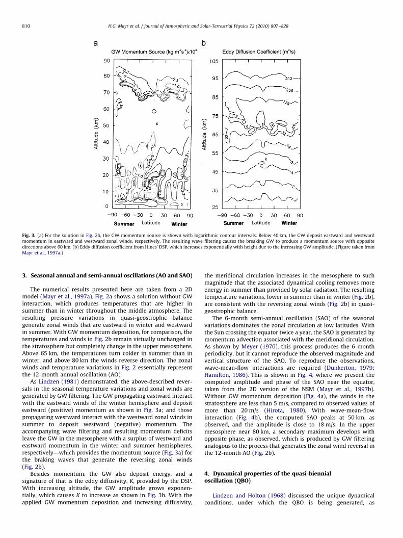
Fig. 3. (a) For the solution in Fig. 2b, the GW momentum source is shown with logarithmic contour intervals. Below 40 km, the GW deposit eastward and westward

momentum in eastward and westward zonal winds, respectively. The resulting wave filtering causes the breaking GW to produce a momentum source with opposite

directions above 60 km. (b) Eddy diffusion coefficient from Hines’ DSP, which increases exponentially with height due to the increasing GW amplitude. (Figure taken from

Mayr et al., 1997a.)


3. Seasonal annual and semi-annual oscillations (AO and SAO)

The numerical results presented here are taken from a 2Dmodel (Mayr et al., 1997a). Fig. 2a shows a solution without GWinteraction, which produces temperatures that are higher insummer than in winter throughout the middle atmosphere. Theresulting pressure variations in quasi-geostrophic balancegenerate zonal winds that are eastward in winter and westwardin summer. With GW momentum deposition, for comparison, thetemperatures and winds in Fig. 2b remain virtually unchanged inthe stratosphere but completely change in the upper mesosphere.Above 65 km, the temperatures turn colder in summer than inwinter, and above 80 km the winds reverse direction. The zonalwinds and temperature variations in Fig. 2 essentially representthe 12-month annual oscillation (AO).

As Lindzen (1981) demonstrated, the above-described rever-sals in the seasonal temperature variations and zonal winds aregenerated by GW filtering. The GW propagating eastward interactwith the eastward winds of the winter hemisphere and depositeastward (positive) momentum as shown in Fig. 3a; and thosepropagating westward interact with the westward zonal winds insummer to deposit westward (negative) momentum. Theaccompanying wave filtering and resulting momentum deficitsleave the GW in the mesosphere with a surplus of westward andeastward momentum in the winter and summer hemispheres,respectively—which provides the momentum source (Fig. 3a) forthe braking waves that generate the reversing zonal winds(Fig. 2b).

Besides momentum, the GW also deposit energy, and asignature of that is the eddy diffusivity, K, provided by the DSP.With increasing altitude, the GW amplitude grows exponen-tially, which causes K to increase as shown in Fig. 3b. With theapplied GW momentum deposition and increasing diffusivity,

the meridional circulation increases in the mesosphere to suchmagnitude that the associated dynamical cooling removes moreenergy in summer than provided by solar radiation. The resultingtemperature variations, lower in summer than in winter (Fig. 2b),are consistent with the reversing zonal winds (Fig. 2b) in quasi-geostrophic balance.

The 6-month semi-annual oscillation (SAO) of the seasonalvariations dominates the zonal circulation at low latitudes. Withthe Sun crossing the equator twice a year, the SAO is generated bymomentum advection associated with the meridional circulation.As shown by Meyer (1970), this process produces the 6-monthperiodicity, but it cannot reproduce the observed magnitude andvertical structure of the SAO. To reproduce the observations,wave-mean-flow interactions are required (Dunkerton, 1979;Hamilton, 1986). This is shown in Fig. 4, where we present thecomputed amplitude and phase of the SAO near the equator,taken from the 2D version of the NSM (Mayr et al., 1997b).Without GW momentum deposition (Fig. 4a), the winds in thestratosphere are less than 5 m/s, compared to observed values ofmore than 20 m/s (Hirota, 1980). With wave-mean-flowinteraction (Fig. 4b), the computed SAO peaks at 50 km, asobserved, and the amplitude is close to 18 m/s. In the uppermesosphere near 80 km, a secondary maximum develops withopposite phase, as observed, which is produced by GW filteringanalogous to the process that generates the zonal wind reversal inthe 12-month AO (Fig. 2b).

4. Dynamical properties of the quasi-biennialoscillation (QBO)

Lindzen and Holton (1968) discussed the unique dynamicalconditions, under which the QBO is being generated, as

ARTICLE IN PRESS

Fig. 4. (a) 2D model results of amplitude and phase of the 6-month semi-annual

oscillation (SAO) zonal winds near the equator computed without GW momentum

deposition. (b) With GW momentum deposition, the wind amplitude peaks in the

stratosphere and is much larger, in rough agreement with observations. With

opposite phase, a secondary maximum develops around 80 km, which is observed.

The SAO is amplified by GW in the stratosphere, and it is generated through wave

filtering in the mesosphere. (Figure taken from Mayr et al., 1997b.)

Fig. 5. (a) 2D model results of zonal winds near the equator (with mean and

annual cycle removed), computed with seasonal variations of solar heating,

produce a QBO with a period of about 21 months and velocities close to 7 m/s in

the lower stratosphere. (b) Without the seasonal heat source, for perpetual

equinox, the QBO-like oscillation has a period of about 17 months and the

amplitude is only about 3 m/s at 30 km. Wave-driven QBO-like wind oscillations

can be generated without time-dependent seasonal heating, but the amplitudes

are much smaller. (Figure taken from Mayr et al., 1998a.)


illuminated by the zonal momentum balance

r @U

@tþ2OsinyrV�Kr @

2U

@r2¼MS, ð1Þ

where r is the mass density; t the time; U, V the zonal andmeridional winds, respectively; y the latitude; r the radialdistance; O the Earth rotation; K the eddy viscosity; and MS thewave momentum deposition. At the equator, y¼0, where theCoriolis force vanishes, the wave drag is very effective because theaccelerated zonal winds are dissipated only by viscosity. Awayfrom the equator, the Coriolis force becomes important, and itgenerates through the zonal winds a meridional circulation. Themeridional winds in turn redistribute and dissipate the zonal flowoscillation, in part through radiative cooling. This property isdisplayed in model simulations with latitude-independent wavesource (e.g., Mengel et al., 1995), later shown also with Fig. 7,which produces QBO zonal winds that still peak at the equator as

observed—and Haynes (1998) provided an analytical discussionof the process involved.

Lindzen and Holton (1968) induced (stimulated) the QBO withthe solar-driven SAO. But Holton and Lindzen (1972) demon-strated that QBO-like oscillations could be generated withoutseasonal variations, and our numerical results confirmed that(Mayr et al., 1998a). This is shown in Fig. 5, where the zonal winds

ARTICLE IN PRESS


with standard heat source (a) are compared with results obtainedfor perpetual equinox (b). With the seasonal variations ofstratospheric solar heating, the QBO zonal winds around 30 kmare much larger. The period in that case is 21 months (Fig. 5a),compared to 17 months for perpetual equinox (Fig. 5b). In theupper stratosphere, the 6-month SAO (Fig. 5a) has an amplitudeof about 20 m/s, while in Fig. 5b the oscillation is much weakerand has a period of 8 months. The differences between the twosolutions are large and show that the seasonal solar heating in thestratosphere affects the QBO extending down to the tropopause.As later shown with a modeling study, this downward influenceplays a prominent role in generating the solar cycle modulation ofthe QBO.

Closely related to the above computer experiment, animportant feature of the QBO mechanism is the nonlinear natureof the wave-mean-flow interaction that drives the oscillation. Dueto the positive nonlinear feedback associated with critical levelabsorption, owing to planetary waves or gravity waves, themomentum deposition is sharply peaked near zonal wind shears,dU/dr. As seen from Fig. 6 and discussed in Mayr et al. (1998a, b)for Hines’ DSP, this impulsive momentum source can berepresented in a form that is, to first order, proportional to the3rd (or odd) power of the velocity gradient, p[dU(o, r)/dr]3,where o is the fundamental frequency of the oscillation. A sourceof this kind generates, besides 3o, the fundamental frequencyitself, o+o�o, and thus it is capable of maintaining theoscillation without an external time-dependent source, asshown in Fig. 5b. In principle, the QBO can be understood asa nonlinear auto-oscillator like the mechanical clock, in whichthe escapement mechanism imparts the impulse to keep thependulum oscillating at the resonance frequency. The reader isreminded that the solar cycle dynamo is also a nonlinear auto-oscillator.

The GW momentum deposition (Fig. 6), which generates thevertical wind shear and vertical wavelength of the flow oscilla-tion, causes the QBO to propagate slowly down under influence ofviscous dissipation. Slow downward propagation is characteristicof wave induced, or wave amplified, flow oscillations. This appliesalso to the hemispherically symmetric equatorial annual oscilla-

Fig. 6. Snapshots of normalized equatorial zonal winds and effective GW

acceleration (divided by mass density and eddy viscosity). Near wind shears,

dU(o, r)/dr, the wave momentum deposition produces sharp peaks owing to the

positive nonlinear feedback associated with critical level absorption. The

momentum source is approximately proportional to (dU(o/dr))n, where n¼3 or

higher odd integer. An impulsive nonlinear source of this kind can generate an

oscillation without external time-dependent forcing, as shown in Fig. 5b.

(Figure taken from Mayr et al., 1999.)

tion and the monthly oscillations, later discussed, respectively,with Figs. 18b and 22.

5. Long-term variations generated by the QBO

While Hines’ GW parameterization allows us to generate theQBO, it comes with uncertainties that produce a variety ofsolutions. Depending on the chosen parameters for the eddydiffusivity, the applied GW wind variance, and the initial altitudewhere the GW are launched, we have generated QBO periodsbetween 21 and 34 months, within the range of observations. Theamplitudes also vary and can reach values close to those observed.

Among our simulations, the 30-month QBO is standing out inpart because it is optimally suited for synchronization by the6-month SAO. This QBO is of particular interest because it pro-duces in the model a 60-month (5-year) semi-decadal oscillation.Such a 5-year oscillation has been observed in stratospheric datasupplied by the National Centers for Environmental Prediction(NCEP) (Mayr et al., 2007a, 2008), which provide also evidencethat this long-term oscillation is tied to a 30-month QBO.

A QBO with period of 30 months was generated with the 2Dversion of the NSM (Mayr et al., 2000), and in Fig. 7 the computedzonal winds are presented. The winds are shown near the equatorvarying with altitude (Fig. 7), and at about 20 km varying withlatitude (Fig. 7b). The 30-month oscillation dominates at 30 kmwith amplitudes close to 20 m/s, and pronounced signatures of the5-year oscillation are seen in the upper stratosphere and meso-sphere. This particular computer solution was generated with alatitude-independent GW source. As shown in Fig. 7b, the zonalwinds still peak at the equator, where the flow momentum is notdissipated by the meridional winds (Lindzen and Holton, 1968).

As illustrated with Fig. 5, the seasonal variations of solarheating affect the QBO significantly. In the case of the 30-monthQBO, this influence is amplified by the unique phase relationshipwith the SAO, illustrated in Fig. 8. In the lower portion of thefigure, the variations are shown for periods of 24 and 30 months,and their positive and negative excursions are connected to thecorresponding excursions of the overlaying SAO. This shows withsolid vertical lines that, in intervals of 15 months, the 30-monthQBO is phase locked to the SAO. With the period of 24 months, incontrast, the SAO is alternating in phase (solid line) or out ofphase (dashed line), making it less effective in synchronizingthe QBO.

We believe that the 5-year oscillation is generated in the modelby the 30-month QBO interacting with the 12-month annualoscillation (AO), which involves GW node filtering. In this mechan-ism, illustrated in Fig. 9, the waves propagating up around the nodesof the QBO are less attenuated and therefore carry more momentum.This enhanced GW momentum flux is applied to amplify the12-month AO in different phases. Since the phase of the AO reversesexactly in time intervals of 30 months, the enhanced wavetransmission around QBO nodes causes amplifications in oppositedirections to yield the 60-month oscillation.

The oscillations associated with this 30-month QBO are shownin Fig. 10, where we present the Fourier spectra for thehemispherically symmetric (a) and anti-symmetric (b) zonalwinds obtained from a 30-year computer run. (For thesymmetric and anti-symmetric components, the winds in theopposite hemispheres have the same and opposite phase,respectively. The anti-symmetric component vanishes at theequator.) In Fig. 10, the amplitudes are presented in terms ofdiscrete Fourier harmonics, h. The corresponding frequencies, o,are then given by h/30 (cycles per year), and the periods are 30/h(years), shown in months. This format is perhaps unusual butis convenient for the present purposes where we interpret the

ARTICLE IN PRESS

Fig. 7. (a) Zonal winds near equator show 30-month QBO, and signatures of 5-year oscillation extending from the stratosphere into the upper mesosphere. (b) At about

20 km, the oscillations are confined to low latitudes, although the GW source is latitude independent. (From a model discussed in Mayr et al., 2000.)

Fig. 8. SAO synchronization of QBO. In intervals of 15 months (vertical solid lines),

the positive and negative phases of the 30-month QBO and SAO coincide. For the

24-month QBO, the SAO is alternating in phase (solid line) and out of phase

(dashed line). (Figure taken from Mayr et al., 1999.)


results in terms of nonlinear interactions. Considering theproduct (P) of the complex amplitudes (A, B), P exp[i(oA7oB)t]¼A exp[ioAt]�B exp[ioBt], nonlinear interactions can be identifiedin the spectra simply from the additions and subtractions offrequencies or integers, i.e., oA7oB-hA7hB. And nonlinearinteractions between hemispherically symmetric (s) and anti-symmetric (a) oscillations in the northern (N) and southern (S)hemispheres produce the products, P(s)¼N(s)� S(s) or P(s)¼N(a)� S(a) and P(a)¼N(s)� S(a), corresponding to the harmonics,h(s)P¼h(s)A7h(s)B or h(s)P¼h(a)A7h(a)B, and h(a)P¼h(a)A7h(s)B,respectively.

Since the 30-month QBO is tightly synchronized by the SAO,the spectral features in Fig. 10 are exceptionally sharp. In Fig. 10a,the 30-month QBO appears at h¼12, and it is hemisphericallysymmetric like the 6-month SAO at h¼60. The 12-month AO,in contrast, is anti-symmetric at h¼30 in Fig. 10b. Generated bythe symmetric QBO interacting with the anti-symmetric AO(illustrated in Fig. 9), the 5-year oscillation is anti-symmetric andoccurs at h¼6 in Fig. 10b. In addition to these oscillations, Fig. 10reveals a number of other spectral features. As identified witharrows, for example, the nonlinear interaction between theanti-symmetric AO and symmetric QBO produces, in Fig. 10b,prominent anti-symmetric amplitudes at h¼30712 with periodsof 8.6 and 20 months. And the anti-symmetric AO and 5-yearoscillation interact to produce the symmetric amplitudes ath¼3076, having periods of 10 and 15 months in Fig. 10a.

The NSM is fully nonlinear, and a number of processes could beinvolved in generating the identified interactions between AO, SAO,QBO, and 5-year oscillation (Fig. 10). In addition to dynamicalinteractions like nonlinear advection and GW node filtering (Fig. 9),we believe that directional gravity wave filtering could alsocontribute as discussed in Mayr et al. (2000). This process isillustrated in Fig. 11 for the interaction between the AO and SAO.In the positive phase of the AO, the eastward propagating GWare preferentially absorbed to produce a surplus of westwardpropagating waves. These waves then interact with the westwardphase of the SAO to amplify it; and directional GW filtering by thenegative phase of the AO amplifies the positive phase of the SAO.

The 30-month QBO with 5-year oscillation is observed todominate in the NCEP data for about 20 years (Mayr et al., 2007a).But the QBO period varies over longer time spans and on average

ARTICLE IN PRESS


is close to 28 years (Baldwin et al., 2001). Given the wide range ofobserved periods between 22 and 34 months, Mayr et al. (2003a)showed how the QBO, in general, could produce long-term varia-tions through wave filtering (illustrated in Fig. 9 for 30-month

Fig. 9. Illustration of GW node filtering, in which the 30-month QBO generates the

60-month (5-year) oscillation through interaction with the 12-month AO. In

intervals of 30 months, between nodes of QBO, the phase of the AO reverses, and

the accompanying wave interaction causes amplification in opposite directions to

generate the long-term variation. (Figure taken from Mayr et al., 2000.)

Fig. 10. Fourier spectra for zonal winds at 111 latitude from a 2D model that generates t

are proportional to frequencies. Nonlinear interactions between spectral features are id

are shown with arrows.

QBO). The generic process for generating such oscillations isillustrated in Fig. 1 of that paper. It requires that in multipleintervals of the QBO period, tB, the phase of the 12-month AO or6-month SAO must reverse to produce the beat period, tB

tB ¼ 2N � tQ ¼ ð2nþ1Þ � 12;6, ð2Þ

he 30-month QBO. Analysis of 30 years is presented in terms of harmonics, h, which

entified from additions and subtractions of harmonics, and the associated periods

Fig. 11. Illustration of nonlinear interaction with directional gravity wave filtering

applied to AO and SAO. Eastward GW are absorbed in the eastward phase of the

AO to produce a surplus of westward waves. The waves in turn interact with, and

amplify, the westward phase of the SAO to produce a nonlinear interaction. (Figure

taken from Mayr et al., 2000.)

ARTICLE IN PRESS


where N and n are integers. For the 30-month QBO with 5-yearbeat period, N¼1 and n¼2. Obeying Eq. (2), our numerical resultsshow that QBO periods of 27 and 22.5 months interact with theAO to produce oscillations of 9 and 15 years, respectively.

6. 3D-model QBO with planetary waves

Employing Hines’ GW parameterization, the QBO solutionsdiscussed above were generated with the 2D version of the NSM.

Fig. 12. 3D computer experiment with GW and planetary waves. (a) Model results with

at 30 km. (b) With inserted Kelvin waves and Rossby gravity waves, the QBO zonal wind

shows that QBO-like oscillations no longer are generated. The isotropic GW source a

generating the QBO in (b).

In 3D, the dynamical situation changes, and we discuss here somenumerical experiments to illustrate that.

In 2D, the GW momentum deposition is solely available forgenerating or amplifying the QBO and SAO, while in 3D the wavesamplify the tides and planetary waves at the expense of theequatorial oscillations. This is shown with a numerical experi-ment (Fig. 8 of Mayr et al., 1999), where we presented 2D and 3Dsolutions with identical GW source. At 30 km, the 2D zonal windsof the QBO are close to 20 m/s, compared to 15 m/s in 3D. And the

weak GW source produces QBO-like oscillations with small zonal winds (o10 m/s)

s increase by more than a factor of 2. (c) Continued model run without GW source

pparently acts as catalyst for the planetary waves to become more effective in

ARTICLE IN PRESS

Fig. 13. 3D model results for 24-month QBO with about 20 m/s winds at 20 km and SAO winds of 30 m/s at 60 km, in reasonable agreement with observations. In addition

to the GW source, assumed to peak at the equator, planetary waves are involved, which are generated by the baroclinic instability in the troposphere. (Figure taken from

Mayr et al., 2009a.)

Fig. 14. Global amplitudes of 24-month QBO oscillation are shown for the hemispherically symmetric components of wind and temperature fields. The QBO zonal winds

(a) are confined to low latitudes and peak in the lower stratosphere. But the meridional winds (b), normalized by scale factor in the left panel, extend to high latitudes to

produce relatively large vertical winds (c) at polar latitudes. Due to adiabatic heating and cooling, large QBO temperature variations (d) are produced in the Polar Regions of

the mesosphere. (Figure taken from Mayr et al., 2009a.)


ARTICLE IN PRESS


differences become larger at higher altitudes, where the tides andplanetary waves grow to large magnitudes.

As shown by Lindzen and Holton (1968), and subsequentlyconfirmed in numerous studies, the QBO can be generated withKelvin waves and Rossby gravity waves. Following Andrews et al.(1987), we also applied this mechanism (Fig. 9 of Mayr et al.,1999). The K-waves occupied the zonal wave numbers 1 and 2and had a period of about 15 days, and the RG-waves with wavenumber m¼4 had a period of 4 days. In contrast to GW, the K- andRG-waves are not naturally constrained to carry the samemomentum flux eastward and westward. The planetary waveshad to be carefully tuned to generate the QBO. Relatively smallchanges in one or the other planetary-wave momentum fluxwould bring the oscillation to a halt.

The differences between the GW and K/RG mechanisms aredisplayed in a numerical experiment presented in Fig. 12. In thetop panel (Fig. 12a), a 3D solution is presented in which the zonalwinds near the equator are generated only with GW. The zonalwinds, eastward red and westward blue, have in the lowerstratosphere small QBO amplitudes below 10 m/s, and the periodis less than 24 months. With identical GW source, the model wasthen run again with excitation of Kelvin and Rossby gravitywaves, and the zonal winds in Fig. 12b reach QBO velocities

Fig. 15. (a) Filtered temperature variations at 85 km, covering the inter-annual varia

considerable differences between the two hemispheres, the QBO amplitudes at high lati

and variable QBO, produce year-to-year variations that can reach 10 K at high latitude

around 20 m/s with a period of more than 30 months. The K/RGmechanism greatly increases the zonal wind oscillations abovethe small values generated with GW. In that light, the solutionpresented in Fig. 12c is then of interest, because it shows that theQBO is no longer generated when the GW are turned off. Thisindicates that the GW act as a catalyst for the planetary waves tobecome more effective in generating the QBO. We believe that theisotropic GW source channels the K/RG mechanism into morebalanced momentum deposition, which is facilitated by thepositive nonlinear feed-back associated with critical levelabsorption (Fig. 6).

As discussed in Mayr et al. (2004), the planetary waves in theNSM are generated internally. For the mesosphere, the analysisshows that the reversing zonal winds and temperature variations,due to GW drag, produce planetary waves through the baroclinicinstability (Plumb, 1983). In the lower atmosphere, the planetarywaves are generated by a time-independent tropospheric heatsource that peaks at the equator. This source produces tempera-tures that peak at the equator in the troposphere but increasetowards higher latitudes in the lower stratosphere, which isobserved. Resembling the dynamical condition in the mesosphere,the latitudinal variations of pressure and temperature haveopposite signs, which is conducive for generating tropospheric

tions with periods above 1 year that describe the variability of the QBO. With

tudes approach 5 K during some years. (b) Filtered temperature variations, AO, SAO

s. (Figure taken from Mayr et al. (2009a.)

ARTICLE IN PRESS

Fig. 16. (a) With period of 10 years, the relative solar cycle (SC) heat input

increases exponentially from 0.2% at the surface to 20% at 100 km and above.

(b) Time constants for eddy viscosity from Hines’ GW parameterization increase in

the lower stratosphere to values above 2 years, which is conducive for generating

SC variations at lower altitudes. (Figure taken from Mayr et al., 2007b.)


planetary waves due to baroclinic instability. The NSM does notdescribe the planetary waves that are generated in GCMs bytopography and tropical convection (e.g., Giorgetta et al., 2002;Horinouchi et al., 2003).

The numerical results presented in the following are takenfrom a 3D model run, which was applied originally in a simulationof the inter-annual variations of the diurnal tide in the uppermesosphere (Mayr and Mengel, 2005). In Fig. 13 we present themonthly average of the zonal winds at 41 latitude near theequator, eastward red and westward blue. With contour intervalsof 5 m/s, it shows that below 40 km the QBO dominates with aperiod of 24 months and amplitudes close to 20 m/s, in roughagreement with observations (e.g., Baldwin et al., 2001). As earliershown for 2D models (Figs. 5a and 7), and observed on UARS(Burrage et al., 1996), the QBO zonal winds from this 3D modelextend into the mesosphere. The 6-month SAO dominates around50 km, with eastward and westward winds near equinox andsolstice respectively, as observed. In agreement with observations(Hirota, 1980), the phase of the SAO reverses in the mesosphere as

earlier shown in Fig. 4b, but in this 3D model the peak occurs at70 instead of 80 km.

QBO temperature oscillations are observed in the mesosphere(Huang et al., 2006b), and in the model they extend across theglobe to the polar mesopause region (Mayr et al., 2009a). This isshown in Fig. 14, where the 24-month amplitudes of thecomputed wind fields and temperature variations are plottedversus altitude and latitude. Allowing 5 years for spin-up, thesubsequent time span of 24 months is Fourier analyzed to derivethe QBO from the first harmonic, and the hemisphericallysymmetric components are presented. Due to the increasingwave drag and eddy viscosity, the meridional and vertical winds(Fig. 14b, c) increase with height exponentially, and they arenormalized by the scale factors on the left.

Fig. 14a shows that the QBO zonal winds peak at the equatorand are largely confined to the stratosphere. The normalizedmeridional winds (Fig. 14b), in contrast, increase into the uppermesosphere and extend with significant magnitude to higherlatitudes. The vertical winds (Fig. 14c), which are part of themeridional circulation, thus attain large amplitudes at polarlatitudes and in particular in the upper mesosphere around 85 km(white circle). The vertical winds cause adiabatic heating andcooling, and this is evident in Fig. 14d, which reveals relativelylarge temperature amplitudes in the polar mesopause region(white circle). As seen in 2D model results, the meridionalcirculation can transfer the temperature signatures of the strato-spheric QBO to the polar regions of the mesosphere (Mayr et al.,2000). But in the present 3D model, the planetary waves wouldalso be involved, which are generated by baroclinic instability inthe troposphere and mesosphere.

In Fig. 15a, we present at 85 km a synthesis (filter) of thetemperature oscillations with periods greater than one year (positivered and negative blue), which produces the inter-annual variationsassociated with the variable QBO. The year-to-year variations canreach 10 K at high latitudes, and the differences between the twohemispheres are large. With a synthesis of the QBO and seasonaloscillations, the temperature variations are shown in Fig. 15b.During the cold summer season, the temperatures typically varyfrom year-to-year by about 5 K, but could reach almost 10 K for theyears 5 and 6 in the north. Such temperature variations wouldcontribute significantly to the observed inter-annual variations ofpolar mesospheric clouds (Thomas, 1991, 1995; Rapp and Thomas,2006).

7. Solar cycle modulated QBO and equatorial annualoscillation (EAO)

In several papers, solar cycle (SC) effects have been linked tothe QBO. One SC connection showed that the temperatures atnorthern polar latitudes in winter are positively and negativelycorrelated with the SC when the QBO is in its negative andpositive phase, respectively (Labitzke, 1982, 1987; Labitzke andVan Loon, 1988, 1992; Dunkerton and Baldwin, 1992; Baldwinand Dunkerton, 1998). The observed correlations have beenreproduced in model simulations (Matthes et al., 2004; Palmerand Gray, 2005).

Related to the model results presented here, the QBO itself isobserved varying with the SC. Applying spectral analysis based ona 41-year data record, Salby and Callaghan (2000) showed that at20 km the filtered SC modulation of the QBO zonal winds varyfrom about 12 to 20 m/s, correlated with the 10.7 cm flux.Analyzing 50 years of wind measurements, Hamilton (2002)confirmed the large QBO modulation but concluded that the SCconnection is not as clear in the extended data record. Corderoand Nathan (2005) showed with a 2D model that the feedback

ARTICLE IN PRESS


from the SC variations of ozone influences the QBO to producevariations that are in phase with the zonal winds observed bySalby and Callaghan (2000).

We believe that the dynamical conditions around the equator,earlier discussed, play a pivotal role in generating the large SCmodulation of the QBO. Due to critical level absorption, verticalwind gradients induce downward propagation of the wind shear,and wave momentum deposition (Fig. 6) amplifies the QBO. Asshown in Fig. 5, the QBO is also amplified by the seasonalvariations of solar heating. These processes figure prominently inour 3D model, which simulates the SC modulation of the QBO(Mayr et al., 2006, 2007b).

The model extends from the ground to about 125 km, and thewave driving is due to parameterized GW and planetary wavesgenerated by the baroclinic instability. The tropospheric GWsource peaks at the equator and is time independent. Asillustrated in Fig. 16a, the applied SC forcing has a period of 10years, and its relative amplitude varies exponentially from 0.2% atthe ground to 20% at 100 km and above. Since the eddy viscosity isdissipating the wave source near the equator, we show in Fig. 16bthe height dependence of the related time constant. Around40 km, it is close to 2 years but increases to more than 10 years at10 km, which is conducive for generating the SC modulation atlower altitudes.

In the 3D model discussed here, the average QBO period ofabout 22 months is at the lower end of the observed range; butthe amplitudes are close to 20 m/s at 30 km. From a computer run

Fig. 17. (a) Power spectrum of symmetric zonal winds for a time span from 10 to 40 yea

at h¼16. The side lobe at h¼13 then represents the 10-year SC modulation, and the one

and 1673, produce the SC modulation of the QBO. It shows that the QBO peaks close

between solar minimum and maximum, a large effect considering the small SC forcing

with SC forcing, we show in Fig. 17a the Fourier power spectrumfor the hemispherically symmetric zonal winds near the equator.Allowing 10 years for spin-up, the time span of 30 years isanalyzed, and it produces at harmonic h¼16 the QBO period of22.5 months. The signature at h¼13 represents the 10-year SCmodulation (and at h¼22 is the 5-year second harmonic). InFig. 17b, we present a synthesis (filter) of h¼16 with 1673,which produces the 10-year SC modulation that causes the windsat 30 km to vary from about 12 to 20 m/s. With solid line, the timedependence of the imposed SC source is shown that peaks at year12.5; it is almost in phase with the QBO modulation. Analysisshows that modulation amplitudes of similar magnitude appearalso in extended computer runs up to 70 years—and we asked thequestion how this large SC effect is transferred to the QBO.

Solar forcing through the seasonal cycles must be involvedin stimulating the QBO modulation, and the model generates a12-month annual oscillation (AO) that is modulated by the SC(Mayr et al., 2005). In the zonal winds, this AO is hemisphericallysymmetric and confined to equatorial latitudes, like the QBO andSAO—and we refer to it as equatorial annual oscillation (EAO).Our analysis shows that the EAO is tied to the seasonal variationsof solar heating in the mesosphere. With constant SC period of 10years, the maximum of the solar cycle occurs during northernsummer solstice, which synchronizes the solar variability and theannual cycle.

Analogous to Fig. 17 for the QBO, we show in Fig. 18 thespectrum and synthesis for the SC modulated symmetric EAO. For

rs. The 3D model with SC forcing generates an average QBO period of 22.5 months

at h¼22 is the 5-year second harmonic. (b) Synthesis of the spectral features, h¼16

to the maximum of SC, and the wind amplitudes vary at 30 km by about 8 m/s

in Fig. 16a. (Figure taken from Mayr et al., 2007b.)

ARTICLE IN PRESS


the 30-year time span analyzed, the dominant feature at h¼30represents the 12-month AO and the one at h¼33 is the signatureof the 10-year modulation. (The 15-year oscillation at h¼32 isgenerated by the 22.5-month QBO interacting with the anti-symmetric AO, as discussed in Section 5.) A synthesis of h¼30with h¼(3073) produces the SC modulation of the EAO, whichpeaks at about 40 km, in phase with the QBO (Fig. 17b) and SCforcing. Like the QBO (Fig. 17b), the symmetric EAO in Fig. 18bslowly propagates down under the influence of wave-mean-flowinteractions. The EAO is apparently the pacemaker and pathwayfor generating the SC modulated QBO.

Wave-mean-flow interactions play a central role in generatingthe above-discussed SC signatures, and this is shown explicitly inFig. 19. We present here the filtered GW momentum deposition(MS) obtained from the 30-year spectral features that describe theSC modulations of the QBO and EAO. Since MS increasesexponentially with height, it is normalized such that at eachaltitude the synthesized maxima are forced to a value chosen tobe 10. For the QBO in Fig. 19a, the MS varies at 40 km by almost afactor of 2, and it varies in phase with the SC. The modulated wavesource for the EAO in Fig. 19b varies by as much as a factor of 4 at40 km, and it is also in phase with the SC.

In the mechanism discussed, the mesospheric SC effect istransferred through the EAO and QBO to lower altitudes bytapping the momentum from the upward propagating GW. Likesteering a powered ocean liner, the energy required to induce theSC modulation in the mesosphere is small when compared with

Fig. 18. Similar to Fig. 17 but showing the 12-month symmetric equatorial annual osci

variations of about 5 m/s in phase with imposed solar source. Like the QBO, the EAO s

(Figure taken from Mayr et al., 2005.)

the energy the waves provide to amplify the flow oscillations atlower altitudes.

The SC modulations of the QBO and EAO extend in thetemperature to the Polar Regions of the troposphere. In Fig. 20, wepresent the filtered temperature variations at 841 latitude,positive red and negative blue. The SC signatures for the QBO(Fig. 20a) are small (o1 K), but they appear in the tropospherebelow 10 km. For the symmetric EAO (Fig. 20b), the temperatureamplitudes of the SC modulation are close to 1 K around 12 km,and the effect appears to propagate down from the stratosphere.We believe that this oscillation could be involved in the so-calledArctic Oscillation, which represents a mode of variability that issensitive to SC influence (e.g., Kodera, 1995; Thompson andWallace, 1998; Baldwin and Dunkerton, 1999; Ruzmaikin andFeynman, 2002).

A symmetric annual oscillation (AO) that peaks at theequator has been observed in NCEP data (Mayr et al., 2007a,2008). Indicative of wave-mean-flow interactions, the slowdownward propagation of the observed EAO agrees withour model results. The observed EAO is modulated by the5-year oscillation that is generated in the model with the30-month QBO, discussed in Section 5. In NCEP data fromthe lower stratosphere, the EAO is modulated with systematicSC signatures (Mayr et al., 2009d). Above 20 km, however, theinferred EAO zonal wind and temperature variations are morevariable, which indicates that SC forcing is not the principal agentat higher altitudes.

llation (EAO) that is modulated by the SC. The SC modulation of the EAO produces

lowly propagates down under the influence of wave-mean-flow interactions.

ARTICLE IN PRESS


8. Monthly intra-seasonal oscillations (ISO)

Wave-mean-flow interactions are very effective in generatingthe QBO, SAO and EAO around the equator, because the zonalwinds involved are divergence-free and do not redistribute energyand momentum to dissipate the oscillations. The monthly intra-seasonal oscillations (ISO) discussed here have in common withthe equatorial zonal wind oscillations that they appear in thezonal mean (m¼0). But in the ISO, the divergent meridional windsare primarily important, which redistribute energy and momen-tum, and this changes the dynamics considerably.

In Fig. 21 we present from a 2D model (Mayr et al., 2003b) thecomputed meridional winds for the middle atmosphere, positivenorthward and negative southward. In the standard solution(Fig. 21a), with isotropic GW source, the waves at the initialheight carry the same momentum in the four principal directions.For comparison, Fig. 21b shows the results obtained without thewaves propagating north/south. Superimposed on the largeannual variations at 80 km, short-term monthly oscillationsappear in Fig. 21a, but not in Fig. 21b without the meridionalsource. And at 50 and 20 km, the monthly ISO dominate (Fig. 21a).

In order to isolate the dynamical process that generatesthe ISO, we present in Fig. 22 a computer solution that isproduced only with the north/south meridional GW momentumdeposition. Fig. 22 reveals a pronounced and regular oscillationwith a period of about 2 months, which propagates down with

Fig. 19. Relative SC modulation of the GW momentum source for QBO (a) and EAO (b

maximum value of 10. In the stratosphere, the momentum sources for QBO and EAO inc

positive nonlinear feedback of the source (Fig. 6), the SC modulations of the equatorial

GW. (Figure taken from Mayr et al., 2007b.)

velocities around 4 km/month. Except for the shorter periodand smaller wind velocities, the oscillation resembles the QBO(e.g., Fig. 7a).

The similarity between this monthly oscillation and the QBO isfurthermore evident in Fig. 23, where snapshots of the heightvariations in the zonal and meridional winds are presented togetherwith the associated momentum depositions. Since the relativevariations are of interest, normalization factors are applied so thatthe quantities can be resolved throughout the middle atmosphere.Fig. 23a describes the dynamical situation for the QBO and SAO, andthe GW source is sharply peaked near zonal wind shears due tocritical level absorption. A similar pattern is also seen in Fig. 23b forthe meridional momentum deposition, in particular at altitudesabove 50 km. In both cases, this impulsive momentum source canbe viewed approximately as a nonlinear function of the velocityfield, U, zonal or meridional, which has the character, (dU/dr)3,of odd power. As discussed in Section 4 for the QBO (Fig. 6),such a nonlinearity can generate an oscillation without externaltime-dependent forcing. The wave-driven zonal and meridionaloscillations, in principle, can be understood as nonlinear auto-oscillator, like the mechanical clock or solar dynamo.

In the case of the QBO, the time constant is closely related tothe eddy diffusivity that dissipates the zonal flow near theequator. For the present monthly oscillations, the divergent wave-driven meridional winds, unlike the zonal wins, generatedynamical heating and cooling, and the resulting pressure

). Since the wave source increases exponentially with height, it is normalized to a

rease from SC minimum to maximum by factors of 2 and 4, respectively. Due to the

QBO and EAO are amplified by tapping the momentum of the upward propagating

ARTICLE IN PRESS


variations counteract and dampen the winds to produce a shorterdissipative time constant. Discussed in Mayr et al. (2003b), thisthermodynamic feedback could explain why the period of the ISOmeridional wind oscillation is much shorter than that of the QBOzonal winds.

In Fig. 24a we present from a 3D model (Mayr et al., 2009b) thecomputed meridional winds at 85 km, positive (red) southward andnegative (blue) northward. The winds peak at the equator and, onaverage, are directed from the summer to the winter hemisphere.As discussed in Section 3, these winds produce at polar latitudes theanomalous temperatures that are lower in summer than in winter(Fig. 24b). Superimposed on the seasonal variations, periods around1.5 months appear, and in Fig. 24c we show the filteredtemperature oscillations with periods from 0.5 to 3 months.Measurable temperature variations are generated around theequator, but the largest amplitudes (�10 K) occur at highlatitudes. The oscillations peak near summer solstice, and thedifferences between the two hemispheres are large. We believe thatthe monthly oscillations of the meridional winds (Fig. 24a) couldproduce, with vertical winds and adiabatic heating/cooling, thetemperature oscillations in Fig. 24c. Monthly temperatureoscillations are also generated with a 2D model (Mayr et al.,2009b). But in the present 3D model, planetary waves would also beinvolved.

Zonal-mean intra-seasonal oscillations (ISO) with periodsaround 1.5 months have been seen in zonal and meridional windsand in the gravity wave activity observed at equatorial latitudes in

Fig. 20. At polar latitudes, measurable SC signatures are generated in the temperatur

(Figure taken from Mayr et al., 2007b.)

the upper mesosphere and lower thermosphere (Eckermann andVincent, 1994; Eckermann et al., 1997). Liebermann (1998),Huang and Reber (2003), and Huang et al. (2005) reported similaroscillations seen in wind measurements on the UARS satellite, andHuang et al. (2006a) inferred such variations from the tempera-ture measurements on the UARS, and on the TIMED spacecraft. Inan analysis of SNOE satellite measurements, Bailey et al. (2005)reported that monthly oscillations occur in the zonal-meanstructure of polar mesospheric clouds (PMC) observed duringthe cold summer season.

The NSM also generates intra-seasonal oscillations in the lowerstratosphere at 30 km (Mayr et al., 2009c). Fig. 25a shows themeridional winds, which reveal pronounced monthly oscillationsthat peak at the equator. The temperatures in the Polar Regionsare higher in summer than in winter and vary with periodsaround 2 months (Fig. 25b). To reveal these oscillations, wepresent in Fig. 25c a filter that portrays the periods between 0.5and 3 months, as in Fig. 24c for the mesosphere. The computedtemperature oscillations vary with season and reach peakamplitudes that approach 5 K after winter solstice, which isqualitatively consistent with the meridional winds in Fig. 25a thatshow such a seasonal pattern at high latitudes.

Intra-seasonal temperature oscillations similar to those pro-duced in the model have been observed in stratospheric NCEPdata (Mayr et al., 2009c), and one of the reviewers (Dr. R.A.Akmaev) of that paper pointed out that the oscillations are relatedto sudden stratospheric warmings (SSW).

e variations of QBO (a) and EAO (b), and they extend down into the troposphere.

ARTICLE IN PRESS


9. Summary

The numerical results discussed were generated with themechanistic Numerical Spectral Model (NSM), which applies Hines’GW parameterization. The model is fully nonlinear and capturesthe generic GW processes of wave filtering and wave-mean-flowinteractions associated with critical level absorption and wavebreaking. The modeling studies presented provide understanding.

For the global-scale annual variations, it is shown that wave-mean-flow interactions accelerate the stratospheric circulation.The momentum deposition of the filtered GW causes the zonalwinds in the mesosphere to reverse, and the temperatures turncolder in summer than in winter, in agreement with observations.In the stratosphere, the GW amplify the 6-month semi-annualoscillation (SAO) at equatorial latitudes, and wave filtering

Fig. 21. (a) 2D model generates in meridional winds zonal-mean (m¼0) intra-season

propagating north/south, the monthly oscillations are not excited. (Figure taken from

produces a secondary maximum in the upper mesosphere withopposite phase, which is observed.

The stratospheric quasi-biennial oscillation (QBO) can begenerated in 2D with GW, and with opposite phase it extendsinto the mesosphere as observed in satellite data. Numericalexperiments show that the QBO can interact with the annual cycleto generate long-term variations through wave filtering andnonlinear interactions. With a QBO period of 30 months, forexample, the model generates a 5-year oscillation that has beenobserved in NCEP data.

Numerical experiments demonstrate that the isotropic GWmomentum deposition channels the planetary-wave source intomore balanced accelerations conducive for generating the QBO.With planetary waves generated by baroclinic instability, the 3Dversion of the NSM produces realistic QBO simulations. The

al oscillations (ISO) with periods around 2 months. (b) Without meridional GW

Mayr et al., 2003b.)

ARTICLE IN PRESS


related inter-annual temperature variations extend into the polarregions of the upper mesosphere and may explain the year-to-year variability observed in PMC.

A 3D modeling study reproduces the large solar cycle (SC)modulation of the QBO zonal winds, which is observed in the lowerstratosphere. The SC effect is transferred to the QBO by a hemi-spherically symmetric equatorial annual oscillation (EAO). Ouranalysis shows that the SC modulations of the QBO and EAO are

Fig. 22. Meridional wind oscillations with periods of about 2 months, which are genera

Fig. 23. Snapshots of zonal (a) and meridional (b) winds and their associated GW mom

interaction causes sharp peaks near vertical wind shears. This nonlinearity is of third (

(Figure taken from Mayr et al., 2003b.)

amplified by GW, and they produce measurable temperaturevariations around the tropopause at high latitudes. A symmetricEAO of the kind generated in the model has been observed in NCEPdata. The EAO is modulated with a 5-year oscillation, and systematicsolar cycle signatures are observed in the lower stratosphere.

In the zonal-mean, the 2D and 3D versions of the NSM producemonthly intra-seasonal oscillations (ISO), which are generatedprimarily by wave interactions with the meridional winds. Unlike

ted only with GW propagating north/south. (Figure taken from Mayr et al., 2003b.)

entum sources. In both wind fields, the nonlinear positive feedback of the wave

odd) power, which enables oscillations without a time-dependent source.

ARTICLE IN PRESS

Fig. 24. (a) Meridional wind oscillations at 85 km generated with a 3D model. Winds extend across the globe but are largest around the equator. (b) Computed temperature

variations, positive red and negative blue, lower in summer than winter, peak in the Polar Regions. Superimposed on the seasonal pattern, monthly oscillations appear.

(c) With Mercator projection, filtered temperature oscillations are shown for periods between 0.5 and 3 months. The largest amplitudes occur at polar latitudes and peak in

summer, with considerable differences between the two hemispheres. (For interpretation of the references to color in this figure legend, the reader is referred to the web

version of this article.) (Figure taken from Mayr et al., 2009b.)


the zonal winds, the meridional winds redistribute energy andmomentum, and the resulting pressure feedback dampens theoscillations to produce periods around 2 months. The meridionalwinds produce relatively large temperature oscillations in thePolar Regions of the mesosphere and stratosphere, varying with

season. In the mesosphere, monthly ISO have been observed intemperature and wind measurements, and in the variability ofPMC. In the stratosphere at high latitudes, the monthly tempera-ture oscillations seen in NCEP data are related to suddenstratospheric warmings (SSW).

ARTICLE IN PRESS

Fig. 25. Similar to Fig. 24 but showing computed meridional wind and temperature variations at 30 km. (a) Winds peak at the equator and extend with small magnitude to

high latitudes. (b) Temperatures are higher in summer than in winter and reveal oscillations with periods around 2 months. (c) Synthesized (filtered) temperature

oscillations for periods between 0.5 and 3 months produce peak amplitudes close to 5 K after winter solstice. (Figure taken from Mayr et al., 2009c.)


Acknowledgements

The authors are indebted to two reviewers whose incisive andconstructive comments contributed significantly to improve thepaper.

References

Akmaev, R.A., 2001a. Simulation of large-scale dynamics in the mesosphere andlower thermosphere with the Doppler-spread parameterization of gravitywaves: 1. Implementation and zonal mean climatologies. J. Geophys. Res. 106,1193–1204.

ARTICLE IN PRESS


Akmaev, R.A., 2001b. Simulation of large-scale dynamics in the mesosphere andlower thermosphere with the Doppler-spread parameterization of gravitywaves: 1. Eddy mixing and diurnal tide. J. Geophys. Res. 106, 1205–1213.

Alexander, M.J., Holton, J.R., Durran, D.R., 1995. The gravity wave response abovedeep convection in a squall line simulation. J. Atmos. Sci. 52, 2212–2226.

Alexander, M.J., Dunkerton, T.J., 1999. A spectral parameterization of mean flowforcing due to breaking gravity waves. J. Atmos. Sci. 52, 2212–2226.

Alexander, M.J., Beres, J.H., Pfister, L., 2000. Tropical stratospheric gravity waveactivity and relationship to clouds. J. Geophys. Res. 105, 22,299–22,309.

Andrews, D.G., Holton, J.R., Leovy, C.B., 1987. Middle Atmosphere Dynamics.Academic Press, San Diego, CA.

Baldwin, M.P., et al., 2001. The quasi-biennial oscillation. Rev. Geophys. 39,179–229.

Baldwin, M.P., Dunkerton, T.J., 1998. Biennial, quasi-biennial, and decadaloscillations of potential vorticity in the northern stratosphere. J. Geophys.Res. 103, 3919–3928.

Baldwin, M.P., Dunkerton, T.J., 1999. Propagation of the Arctic Oscillation fromthe stratosphere to the troposphere. J. Geophys. Res. 104, 30,937.

Bailey, S.M., Merkel, A.W., Thomas, G.E., Carstens, J.N., 2005. Observations of polarmesospheric clouds by the Student Nitric Oxide Explorer. J. Geophys. Res. 110,D13203, doi:10.1029/2004JD005422.

Becker, E., McLandress, C., 2009. Consistent scale interaction of gravity waves inthe Doppler Spread Parameterization. J. Atmos. Sci. 66, 1434–1449.

Burrage, M.D., Vincent, R.A., Mayr, H.G., Skinner, W.R., Arnold, N.F., Hays, P.B.,1996. Long-term variability in the equatorial middle atmosphere winds.J. Geophys. Res. 101, 12,847.

Chan, K.L., Mayr, H.G., Mengel, J.G., Harris, I., 1994a. A ‘stratified’ spectral modelfor stable and convective atmospheres’. J. Comput. Phys. 113, 165.

Chan, K.L., Mayr, H.G., Mengel, J.G., Harris, I., 1994b. A spectral approach forstudying middle and upper atmospheric phenomena. J. Atmos. Terr. Phys. 56,1399.

Charron, M., Manzini, E., Warner, C.D., 2002. Intercomparison of gravity waveparameterizations: Hines Doppler-spread and Warner and McIntyre ultra-simple schemes. J. Meteor. Soc. Jpn. 80, 335–345.

Cordero, E.C., Nathan, T.R., 2005. A new pathway for communicatinghe 11-year solar cycle to the QBO. Geophys. Res. Lett. 32, L18805,doi:10.1029/2005GL023696.

Dunkerton, T.J., 1979. On the role of the Kelvin wave in the westerly phase of thesemiannual zonal wind oscillation. J. Atmos. Sci. 36, 32.

Dunkerton, T.J., 1982. Theory of the mesopause semiannual oscillation. J. Atmos.Sci. 39, 2681.

Dunkerton, T.J., 1985. A two-dimensional model of the quasi-biennial oscillation.J. Atmos. Sci. 42, 1151.

Dunkerton, T.J., 1997. The role of the gravity waves in the quasi-biennialoscillation. J. Geophys. Res. 102, 26,053.

Dunkerton, T.J., Baldwin, M.P., 1992. Modes of interannual variability in thestratosphere. Geophys. Res. Lett. 19, 49–51.

Eckermann, S.D., Vincent, R.A., 1994. First observations of intra-seasonaloscillations in the equatorial mesosphere and lower thermosphere. Geophys.Res. Lett. 21, 265–268.

Eckermann, S.D., Rayopadhyaya, D.K., Vincent, R.A., 1997. Intraseasonal windvariability in the equatorial mesosphere and lower thermosphere: long-term observations from the central pacific. J. Atmos. Solar Terr. Phys. 59,603–627.

Forbes, J.M., Garrett, H.B., 1978. Thermal excitation of atmospheric tides due toinsolation absorption by O3 and H2O. Geophys. Res. Lett. 5, 1013.

Francis, S.H., 1975. Global propagation of atmospheric gravity waves: a review.J. Atmos. Terr. Phys. 37, 1011.

Fritts, D.C., 1982. Shear Excitation of atmospheric gravity waves. J. Atmos. Sci. 39,1936–1952.

Fritts, D.C., 1984. Gravity wave saturation in the middle atmosphere: a review oftheory and observations. Rev. Geophys. 22 (3), 275–308.

Fritts, D.C., 1989. A review of gravity wave saturation processes, effects andvariability in the middle atmosphere. Pure Appl. Geophys. 130, 343–371.

Fritts, D.C., Lu, W., 1993. Spectral estimates of gravity wave energy andmomentum fluxes. II. Parameterization of wave forcing and variability. J.Atmos. Sci. 50, 3695–3712.

Fritts, D.C., Alexander, M.J., 2003. Gravity wave dynamics and effects in the middleatmosphere. Rev. Geophys. 41 (1), 1003, doi:10.1029/2001RG000106.

Garcia, R.R., Solomon, S., 1983. A numerical model of the zonally averageddynamical and chemical structure of the middle atmosphere. J. Geophys. Res.88, 1379.

Garcia, R.R., Solomon, S., 1985. The effect of breaking gravity waves on thedynamics and chemical composition of the mesosphere and lower thermo-sphere. J. Geophys. Res. 90, 3850.

Geller, M.A., 1983. Dynamics of the middle atmosphere. Space Sci. Rev. 34,359–375.

Geller, M.A., 1984. Modeling the middle atmosphere circulation. In: Holton, J.R.,Matsuno, D. (Eds.), Dynamics of the Middle Atmosphere. Terrapub, Tokyo,pp. 467.

Geller, M.A., Shen, W., Zhang, M., Tan, W., 1997. Calculations of the stratosphericquasi-biennial oscillation for time varying wave forcing. J. Atmos. Sci. 54,883–894.

Giorgetta, M.A., Manzini, E., Roeckner, E., 2002. Forcing of the quasi-biennialoscillation from a broad spectrum of atmospheric waves. Geophys. Res. Lett.29, doi:10.1029/2002GL014756.

Hamilton, K., 1986. Dynamics of the stratospheric semi-annual oscillation.J. Meteorol. Soc. Jpn. 64, 227.

Hamilton, K., 2002. On the Quasi-decadal modulation of the stratospheric QBOperiod. J. Clim. 15, 2562.

Hamilton, K., Wilson, R.J., Mahlman, D.J., Umscheid, L.J., 1995. Climatology of theSKYHI troposphere–stratosphere–mesosphere general circulation model.J. Atmos. Sci. 52, 5–43.

Hamilton, K., Wilson, R.J., Hemler, R.S., 2001. Spontaneous stratospheric QBO-likeoscillation simulated by the GFDL SKYHI general circulation model. J. Atmos.Sci. 58, 3271–3292.

Haynes, P.H., 1998. The latitudinal structure of the quasi-biennial oscillation. Q. J.R. Meteorol. Soc. 124, 2645.

Hines, C.O., 1991a. The saturation of gravity waves in the middle atmosphere, I,Critique of linear-instability theory. J. Atmos. Sci. 48, 1348–1360.

Hines, C.O., 1991b. The saturation of gravity waves in the middle atmosphere, II,Development of Doppler-spread theory. J. Atmos. Sci. 48, 1361–1379.

Hines, C.O., 1991c. The saturation of gravity waves in the middle atmosphere, III,Formulation of the turbopause and of turbulent layers beneath it. J. Atmos. Sci.48, 1380–1386.

Hines, C.O., 1993. The saturation of gravity waves in the middle atmosphere, IV,Cut-off of the incident wave spectrum. J. Atmos. Sci. 50, 3045–3060.

Hines, C.O., 1996. Nonlinearity of gravity-wave saturated spectra in the middleatmosphere. Geophys. Res. Lett. 23, 3309–3312.

Hines, C.O., 1997a. Doppler-spread parameterization of gravity-wave momentumdeposition in the middle atmosphere, 1, Basic formulation. J. Atmos. Solar Terr.Phys. 59, 371–386.

Hines, C.O., 1997b. Doppler-spread parameterization of gravity-wave momentumdeposition in the middle atmosphere, 2, Broad and quasi monochromaticspectra, and implementation. J. Atmos. Solar Terr. Phys. 59, 387–400.

Hines, C.O., 1999. Correction to ‘‘Doppler-spread parameterization of gravity-wavemomentum deposition in the middle atmosphere, 1, Basic formulation’’[Journal of Atmospheric and Solar–Terrestrial Physics, 59 (1997) 371–386]. J.Atmos. Solar Terr. Phys. 61, 941.

Hines, C.O., 2001. Theory of the Eulerian tail in the spectra of atmospheric andoceanic internal gravity waves. J. Fluid Mech. 448, 289–313.

Hines, C., 2002. Nonlinearities and linearities in internal gravity waves of theatmosphere and the oceans. Geophys. Astrophys. Fluid 96, 1–30.

Hirota, I., 1980. Observational evidence of the semiannual oscillationin the tropical middle atmosphere—a review. Pure Appl. Geophys. 118,217–238.

Hitchman, M.H., Leovy, C.B., 1988. Estimation of the Kelvin wave contribution tothe semiannual oscillation. J. Atmos. Sci. 45, 1462–1475.

Hocke, K., Schlegel, K., 1996. A review of atmospheric gravity waves and travelingionospheric disturbances: 1982–1995. Ann. Geophys. 14, 914–940.

Holton, J.R., 1982. The role of gravity wave induced drag and diffusion in themomentum budget of the mesosphere. J. Atmos. Sci. 39, 791.

Holton, J.R., Lindzen, R.S., 1972. An updated theory for the quasi-biennial cycle ofthe tropical stratosphere. J. Atmos. Sci. 29, 1076.

Holton, J.R., Zhu, X., 1984. A further study of gravity wave induced drag anddiffusion in the mesosphere. J. Atmos. Sci. 41, 2653–2662.

Holton, J.R., Alexander, M.J., 2000. The role of waves in the transport circulation ofthe middle atmosphere, Atmospheric Science Across the Stratosphere. AGU,Washington, DC.

Horinouchi, T., Pawson, S., Shibata, K., Langematz, U., Manzini, E., Giorgetta, M.,Sassi, F., Wilson, R., Hamilton, K., De Grandpre, J., Scaife, A., 2003. Tropicalcumulus convection and upward-propagating waves in middle-atmosphericGCMs. J. Atmos. Sci. 60, 2765–2782.

Huang, F.T., Reber, C.A., 2003. Seasonal behavior of the semidiurnal and diurnaltides, and mean flows at 95 km, based on measurements from the HighResolution Doppler Imager (HRDI) on the Upper Atmosphere Research Satellite(UARS). J. Geophys. Res. 108, 4360, doi:10.1029/2002JD003189.

Huang, F.T., Mayr, H.G., Reber, C.A., 2005. Intra-seasonal Oscillations (ISO) of zonalmean meridional winds and temperatures as measured by UARS. Ann.Geophys. 23, 1131–1137.

Huang, F.T., Mayr, H.G., Reber, C.A., Russell, J., Mlynczak, M., Mengel, J., 2006a.Zonal-mean temperature variations inferred from SABER measurements onTIMED compared with UARS observations. J. Geophys. Res. 111, A10S07,doi:10.1029/2005JA011427.

Huang, F.T., Mayr, H.G., Reber, C.A., Russell, J., Mlynczak, M., Mengel, J., 2006b.Stratospheric and mesospheric temperature variations for the quasi biennialand semiannual (QBO and SAO) oscillations based on measurements fromSABER (TIMED) and MLS (UARS). Ann. Geophys. 24, 2131–2149.

Kodera, K., 1995. On the origin and nature of the interannual variability of thewinter stratospheric circulation in the northern hemisphere. J. Geophys. Res.100, 14077–14088.

Labitzke, K., 1982. On the inter-annual variability of the middle stratosphereduring northern winters. J. Meteorol. Soc. Jpn. 60, 124–139.

Labitzke, K., 1987. Sunspots, the QBO and stratospheric temperature in the northpolar region. Geophys. Res. Lett. 14, 535–537.

Labitzke, K., Van Loon, H., 1988. Association between the 11-year solar cycle,the QBO and the atmosphere. Part I: the troposphere and stratosphere in thenorthern hemisphere in winter. J. Atmos. Terr. Phys. 50, 197–206.

Labitzke, K., Van Loon, H., 1992. On the association between the QBO and theextratropical stratosphere. J. Atmos. Terr. Phys. 54, 1453–1463.

Lawrence, B.N., 2001. A gravity-wave induced quasi-biennial oscillation in a three-dimensional mechanistic model. Q. J. R. Meteorol. Soc. 127, 2005–2021.

dx.doi.org/10.1029/2004JD005422.3d

dx.doi.org/10.1029/2005GL023696.3d

dx.doi.org/10.1029/2001RG000106.3d

dx.doi.org/10.1029/2002GL014756.3d

dx.doi.org/10.1029/2002JD003189.3d

dx.doi.org/10.1029/2005JA011427.3d

ARTICLE IN PRESS


Lieberman, R.S., 1998. Intraseasonal variability of high-resolution Doppler imagerwinds in the equatorial mesosphere and lower thermosphere. J. Geophys. Res.103, 11,221–11,228.

Lindzen, R.S., Holton, J.R., 1968. A theory of the quasi-biennial oscillation. J. Atmos.Sci. 25 (1095), 1968.

Lindzen, R.S., 1981. Turbulence and stress due to gravity wave and tidalbreakdown. J. Geophys. Res. 86, 9707.

Manzini, E., McFarlane, N.A., McLandress, C., 1997. Impact of the Doppler spreadparameterization on the simulation of the middle atmosphere circulationusing the MA/ECHQAM4 general circulation model. J. Geophys. Res. 102,25751.

Matthes, K., Langematz, U., Gray, L., Kodera, K., Labitzke, K., 2004. Improved11-year solar signal in the Freie Universitaet Berlin, Limate Middle Atmo-sphere Model (FUB-CMAM). J. Geophys. Res. 109, D06101, doi:10.1029/2003JD004012.

Mayr, H.G., Mengel, J.G., Hines, C.O., Chan, K.L., Arnold, N.F., Reddy, C.A., Porter,H.S., 1997a. The gravity wave Doppler spread theory applied in a numericalspectral model of the middle atmosphere, 1, Model and global-scale seasonalvariations. J. Geophys. Res. 102, 26,077.

Mayr, H.G., Mengel, J.G., Hines, C.O., Chan, K.L., Arnold, N.F., Reddy, C.A., Porter,H.S., 1997b. The gravity wave Doppler spread theory applied in a numericalspectral model of the middle atmosphere, 2, Equatorial oscillations. J. Geophys.Res. 102, 26,093.

Mayr, H.G., Mengel, J.G., Chan, K.L., 1998a. Equatorial oscillations maintained bygravity waves as described with the Doppler Spread Parameterization: I.Numerical experiments. J. Atmos. Solar Terr. Phys. 60, 181.

Mayr, H.G., Mengel, J.G., Chan, K.L., 1998b. Equatorial oscillations maintained bygravity waves as described with the Doppler Spread Parameterization: I.Heuristic analysis. J. Atmos. Solar Terr. Phys. 60, 201.

Mayr, H.G., Mengel, J.G., Reddy, C.A., Chan, Porter, H.S., 1999. The role of gravitywaves in maintaining the QBO and SAO at equatorial latitudes. Adv. Space Res.11, 1531.

Mayr, H.G., Mengel, J.G., Reddy, C.A., Chan, K.L., Porter, H.S., 2000. Properties ofQBO and SAO generated by gravity waves. J. Atmos. Solar Terr. Phys. 62,1135–1154.

Mayr, H.G., Mengel, J.G., Drob, D.P., Chan, K.L., Porter, H.S., 2003a. Modeling studieswith QBO: I, Quasi decadal oscillation. J. Atmos. Solar Terr. Phys. 65, 887.

Mayr, H.G., Mengel, J.G., Drob, D.P., Porter, H.S., Chan, K.L., 2003b. Intraseasonaloscillations in the middle atmosphere forced by gravity waves. J. Atmos. SolarTerr. Phys. 65, 1187.

Mayr, H.G., Mengel, J.G., Talaat, E.R., Porter, H.S., Chan, K.L., 2004. Modeling studyof mesospheric planetary waves: genesis and characteristics. Ann. Geophys.22, 1885.

Mayr, H.G., Mengel, J.G., 2005. Inter-annual variations of the diurnal tide in themesosphere generated by the quasi-biennial oscillation. J. Geophys. Res. 110,D10111, doi:10.1029/2004JD005055.

Mayr, H.G., Mengel, J.G., Wolff, C.L., 2005. Wave-driven equatorial annualoscillation induced and modulated by the solar cycle. Geophys. Res. Lett. 32,L20811.

Mayr, H.G., Mengel, J.G., Wolff, C.L., Porter, H.S., 2006. QBO as potential amplifier ofsolar cycle influence. Geophys. Res. Lett. 33, L05812.

Mayr, H.G., Mengel, J.G., Huang, F.T., Nash, E.R., 2007a. Equatorial annualoscillation with QBO-driven 5-year modulation in NCEP data. Ann. Geophys.25, 37–45.

Mayr, H.G., Mengel, Wolff, C.L., Huang, F.T., Porter, H.S., 2007b. The QBO aspotential amplifier and conduit to lower altitudes of solar cycle influence. Ann.Geophys. 25, 1071–1092.

Mayr, H.G., Mengel, J.G., Huang, F.T., Talaat, E.R., Nash, E.R., Reddy, C.A., 2008.Stratospheric semi-decadal oscillations in NCEP data. Ann. Geophys. 26,2143–2157.

Mayr, H.G., Mengel, J.G., Huang, F.T., 2009a. Modeling the temperature of the polarmesopause region: Part I—Inter-annual and long-term variations generated bythe stratospheric QBO. J. Atmos. Solar Terr. Phys. 71, 497–507.

Mayr, H.G., Mengel, J.G., Huang, F.T., Bailey, S.M., 2009b. Modeling thetemperature of the polar mesopause region: Part II—Intra-seasonal monthlyoscillations. J. Atmos. Solar Terr. Phys. 71, 508–517.

Mayr, H.G., Mengel, J.G., Huang, F.T., Nash, E.R., 2009c. Intra-seasonal monthlyoscillations in stratospheric NCEP data and model results. J. Atmos. Solar Terr.Phys. 71, 1508–1517.

Mayr, H.G., Mengel, J.G., Huang, F.T., Nash, E.R., 2009d. Solar cycle signatures in theNCEP equatorial annual oscillation. Ann. Geophys. 27, 3225–3235.

McLandress, C., 2002a. The seasonal variation of the propagating diurnal tide inthe mesosphere and lower thermosphere. Part I: The role of gravity waves andplanetary waves. J. Atmos. Sci. 59, 893–906.

McLandress, C., 2002b. Interannual variations of the diurnal tide in themesosphere induced by a zonal-mean wind oscillation in the tropics. Geophys.Res. Lett. 29 (9, doi:10.1029/201GL014551.

Medvedev, A.S., Klassen, G.P., 2000. Parameterization of gravity wave momentumdeposition based on nonlinear wave interactions: basic formulation andsensitivity tests. J. Atmos. Solar Terr. Phys. 62, 1015–1033.

Mengel, J.G., Mayr, H.G., Chan, K.L., Hines, C.O., Reddy, C.A., Arnold, N.F., Porter,H.S., 1995. Equatorial oscillations in the middle atmosphere generated bysmall scale gravity waves. Geophys. Res. Lett. 22, 3027.

Meyer, W.D., 1970. A diagnostic numerical study of the semiannual variations ofthe zonal wind in the tropical stratosphere and mesosphere. J. Atmos. Sci. 27,820.

Palmer, M., Gray, L., 2005. Modeling the atmospheric response to solar irradiancechanges using a GCM with a realistic QBO. Geophys. Res. Lett. 32, L24701,doi:10.1029/2005GL023809.

Pascoe, C.L., Gray, L.C., Crooks, S.A., Jukes, M.N., Baldwin, M.P., 2005. The quasi-biennial oscillation: analysis using ERA-40 data. J. Geophys. Res. 110, D08105,doi:10.1029/2004JD004941.

Plumb, R.A., 1977. The interaction of two internal waves with the meanflow: implications for the theory of the quasi-biennial oscillation. J. Atmos. Sci.34, 1847.

Plumb, R.A., 1983. Baroclinic instability of the summer mesosphere: a mechanismfor the quas-2-day wave? J. Atmos. Sci. 40 262.

Rapp, M., Thomas, C.E., 2006. Modeling the microphysics of mesospheric iceparticles: assessment of current capabilities and basic sensitivities. J. Atmos.Sol. Terr. Phys. 68, 715.

Ruzmaikin, A., Feynman, J., 2002. Solar influence on a major mode of atmosphericvariability. J. Geophys. Res., 107, doi:10.1029/2001JD001239.

Salby, M., Callaghan, P., 2000. Connection between the solar cycle and the QBO: themissing link. J. Clim. 13, 2652–2662.

Scaife, A.A., Butchart, N., Warner, C.D., Swinbank, R., 2002. Impact of a spectralgravity wave parameterization on the stratosphere in the Met Office UnifiedModel. J. Atmos. Sci. 59, 1473–1489.

Schoeberl, M.R., 1985. A ray tracing model of gravity wave propagation andbreakdown in the middle atmosphere. J. Geophys. Res. 90, 7999–8010.

Schoeberl, M.R., Strobel, D.F., Apruzese, J.P., 1983. A numerical model ofgravity wave breaking and stress in the mesosphere. J. Geophys. Res. 88,5249–5259.

Strobel, D.F., 1978. Parameterization of atmospheric heating rate from 15 to 120km due to O2 and O3 absorption of solar radiation. J. Geophys. Res. 83, 7963.

Takahashi, M., 1999. Simulation of the quasi-biennial oscillation in a generalcirculation model. Geophys. Res. Lett. 26, 1307.

Thomas, G.E., 1991. Mesospheric clouds and the physics of the mesopause region.Rev. Geophys. 29, 553–575.

Thomas, G.E., 1995. Climatology of polar mesospheric clouds: interannualvariability and implications for long-term trends. Geophys. Monograph 87,185–200.

Thompson, D.W.J., Wallace, J.M., 1998. The Arctic Oscillation signature in thewintertime geopotential height and temperature fields. Geophys. Res. Lett. 25(11297), 1998.

Vadas, S.L., Fritts, D.C., 2002. The importance of spatial variability in the generationof secondary gravity waves from local body forces. Geophys. Res. Lett., 29,doi:10.1029/2002GL015574.

Vadas, S.L., Fritts, D.C., Alexander, J.M., 2003. Mechanism for the generation ofsecondary waves in wave breaking regions. J. Atmos. Sci. 60, 94–214.

Warner, C.D., McIntyre, M.E., 2001. An ultrasimple spectral parameterization fornonorographic gravity waves. J. Atmos. Sci. 58, 1837–1857.

Wehrbein, W.M., Leovy, C.B., 1982. An accurate radiative heating and coolingalgorithm for use in a dynamical model of the middle atmosphere. J. Geophys.Res. 39, 1532.

Zhu, X., 1987. On gravity wave-mean flow interaction in a three dimensionalstratified atmosphere. Adv. Atmos. Sci. 4, 287–299.

Zhu, X., 1989. Radiative cooling calculated by random band models with S-1-betatailed distribution. J. Atmos. Sci. 46, 511.

Zhu, X., Yee, J.-H., Swartz, W.H., Talaat, E.R., Lawrence C. A spectral parameteriza-tion of drag, eddy diffusion, and wave heating for a three-dimensionalflow induced by breaking gravity waves. J. Atmos. Sci., accepted forpublication.

dx.doi.org/10.1029/2003JD004012.3d

dx.doi.org/10.1029/2003JD004012.3d

dx.doi.org/10.1029/2004JD005055.3d

dx.doi.org/10.1029/201GL014551.3d

dx.doi.org/10.1029/2005GL023809.3d

dx.doi.org/10.1029/2004JD004941.3d

dx.doi.org/10.1029/2001JD001239.3d

dx.doi.org/10.1029/2002GL015574.3d

middle atmosphere dynamics with gravity wave interactions in the numerical spectral model:...

Documents