455

Microwave temperature andpressure measurements with theOdin satellite: II. Retrieval method

M. Ridal, D.P. Murtagh, F. Merino, J.R. Pardo, and L. Pagani

Abstract: The millimetre receiver on the Swedish satellite Odin, will be used for detectionof the 118.750 GHz oxygen line. The temperature and pressure will be determined from theoutput of a three-channel filter bank measurement. One frequency bin is centred over theemission-line frequency while the other two cover parts of the line wing, where the opacity isless, providing a useful signal at lower altitudes. The bandwidth of each channel is 40 MHz.The signal in the frequency bin covering the line centre is modeled by a high-resolutionmodel including the Zeeman effect, developed by the Observatoire de Paris–Meudon. Theother two 40 MHz bins are modeled using the much faster standard Odin forward model,developed at the Department of Meteorology at Stockholm University together with ChalmersUniversity of Technology. The operational retrievals employ an iterative method that usessimulated signals from a reference atmosphere as a lookup table for the pressure. Thetemperature is then calculated from the equation of hydrostatic equilibrium, and a new lookuptable computed. This process is repeated until a convergence criterion is reached. Simulations,including known error sources, show that the temperature can be retrieved with a root meansquare (rms) around 3 K, in the altitude range∼25–90 km using the operational temperatureretrieval method (the filter bank method). A sub-millimetre receiver on board Odin will alsobe used to observe the oxygen line at 487.249 GHz. Both this line and the 118.750 GHz linecan be observed in high resolution (150 kHz) for detailed studies of the Zeeman splitting.Retrievals from the high-resolution measurements are expected to give a precision of±2 Krms at that resolution. However, this kind of observation will occupy an entire spectrometerand will not be made on a regular basis.

Received 1 May 1999. Accepted 15 January 2001. Published on the NRC Research Press Web site athttp://cjp.nrc.ca/ on 18 April 2002.

M. Ridal, 1,2 D.P. Murtagh,3 and F. Merino. Department of Meteorology, Svante Arrhenius v. 12, StockholmUniversity, SE-10691 Stockholm, Sweden.J.R. Pardo.4 DEMIRM, UMR 8540, Observatoire de Paris-Meudon, 61 avenue de l’Observatoire, 75014 Paris,France; NASA-Goddard Institute for Space Studies, 2880 Broadway, NewYork, NY 10025, U.S.A.; and GeorgeW. Downs Laboratory of Physics, MS 320-47, California Institute of Technology, 1200 E California Blvd.,Pasadena, CA 91125, U.S.A.L. Pagani.DEMIRM, URA 336 du CNRS, Observatoire de Paris-Meudon, 61 avenue de l’Observatoire, 75014Paris, France.

1Corresponding author (email: martin@smhi.se).2Present Address: SMHI (Swedish Meteorological and Hydrological Institute), SE-601 76 Norrköping,Sweden.

3Present Address: Department of Radio and Space Science, Chalmers University of Technology, SE-41296Göteborg, Sweden.

4Present Address: Consejo Superior de Investigaciones Cientificas, IEM, Serrano 121, E-28006, Madrid,Spain.

Can. J. Phys.80: 455–467 (2002) DOI: 10.1139/P02-021 © 2002 NRC Canada

456 Can. J. Phys. Vol. 80, 2002

PACS Nos.: 07.57Yb, 94.10Dy, 95.75Rs

Résumé: Le récepteur millimétrique du satellite Odin a pour mission de détecter la raieà 118,750 GHz de l’oxygène. Une batterie de filtres à trois canaux permet de déterminerla température et la pression. Une des fenêtres en fréquence est centrée sur le milieu dela raie d’émission, alors que les deux autres couvrent les ailes où l’opacité est plus faible,fournissant un signal utile à basse altitude. La largeur de chaque canal est 40 MHz. Lesignal dans le canal central est modélisé par un modèle à haute résolution développé àl’Observatoire de Paris-Meudon et tient compte de l’effet Zeeman. Les signaux des deuxcanaux latéraux sont modélisés par le modèle standard Odin qui est beaucoup plus rapidede calcul et qui a été développé par le département de Météorologie de l’Université deStockholm avec l’Université technique de Chalmers. Les résultats sont recouvrés par uneméthode itérative qui utilise le signal simulé d’une atmosphère de référence comme tablede recherche pour déterminer la pression. On calcule alors la température à l’aide del’équation d’équilibre hydrostatique et une nouvelle table est générée. On répète le processusjusqu’à convergence. Des simulations, incluant les sources connues d’erreur montrent que latempérature peut être déterminée avec une valeur rms de 3 K, aux altitudes variant de 25 à90 km avec la procedure normale d’observation. Un détecteur submillimétrique à bord d’Odina comme mission d’observer la raie de l’oxygène à 487,249 GHz. Ces deux raies peuventêtre observées à haute résolution (150 kHz) pour une étude détaillée de la séparation Zeeman.Le traitement de l’ensemble de ces mesures à haute résolution devrait mener à une précisionde ±2 K rms. Cependant, cela requiert l’utilisation en continu d’un spectromètre et ne seradonc pas fait sur une base continue.

[Traduit par la Rédaction]

1. Introduction

Odin is the third in a series of small Swedish satellites. Odin has been built in collaboration withCanada, Finland, and France, and will measure a number of atmospheric constituents for studies ofmiddle-atmospheric chemistry and the dynamics of the stratosphere and mesosphere. The spacecraftis equipped with two instruments, a millimetre–sub-millimetre receiver (SMR) for both atmosphericand astronomical measurements and an optical instrument (OSIRIS) that is only used for aeronomymeasurements [1].

Measurements of temperature and pressure using the 118.75 GHz O2 line will be performed by theSMR instrument. The routine measurements of the thermal emissions from this oxygen line will bemade in three fixed-frequency filters (filter bank), one covering the line centre and two further out inthe line wings. There is also the possibility of using a high-resolution spectrometer for measurementsof this and the 487.25 GHz oxygen line. The two different measurement modes are described in detailin Pardo et al. [2].

A complicating feature of the atmospheric oxygen lines is the Zeeman-splitting effect.The permanentmagnetic dipole of the O2 molecule interacts with the Earth’s geomagnetic field and causes a splittingof the rotational energy levels. Below 60 km the Zeeman splitting is negligible compared to the pressurebroadening of the line. Further, the high rate of collisions effectively prevents the magnetic dipolesfrom orientating along the direction of the magnetic field. Above∼60 km however, this effect becomessignificant and needs to be taken into account when simulating O2 spectra [2,3].

This work describes a retrieval method specifically designed for the filter bank measurements withthe SMR instrument.The method, developed at the Department of Meteorology at Stockholm University,is similar to the method used to retrieve temperature and pressure from LIMS data [4].

In this paper, we first outline the physical requirements (Sect. 2) needed for the retrieval of tem-perature and pressure. The forward models used for simulating the satellite signals and for use in theretrieval models are fully described in ref. 2 but for completeness, briefly described in Sect. 3. Section4 then follows with a short description of the different O2 measurement modes. In Sect. 5, we describethe retrieval methods, the operational in detail and the high-resolution retrieval briefly. A few examples

©2002 NRC Canada

Ridal et al. 457

of retrieved profiles follow in Sect. 6. We will also, in the last section, estimate the size of the main errorsources and the effect they will have on the retrievals.

2. Physical precepts

Under the assumption that local thermodynamic equilibrium (LTE) applies, the radiation,I , comingfrom an atmospheric constituent is dependent on the amount of gas, the properties of the molecule, andthe local temperature [5] according to

I = B(T )Nε dl (1)

whereB(T ) is the blackbody function for temperature(T ), N is the number density of the emittinggas andε includes the properties of the molecule and of the absorption line in use, dl is the path lengththrough the gas in which the measurement took place. The productNε is commonly known as theabsorption coefficient.

The retrieval of the unknown mixing ratios of different atmospheric molecules thus requires apriori knowledge of the temperature. This required information can come from either climatologicaltemperature and pressure profiles or from local simultaneous measurements. The latter are preferredsince they are expected to give more accurate information than the climatology. The temperature itselfcan be derived from measurements of atmospheric species with well-known mixing ratios. Moleculeswith known mixing ratios are for example O2 and CO2. These have been used frequently in temperaturemeasurements from satellites to determine the atmospheric temperature and pressure, see, for example,refs. 6–8.

A further assumption that has to be made is that the atmosphere is in hydrostatic equilibrium.Otherwise one cannot relate the pressure and temperature to each other.

Two advantages with using the 118.75 GHz oxygen line is that the wavelength is long enough for thescattered solar radiation to be negligible and there are no “disturbing lines” that will affect the measuredsignal significantly.

2.1. Zeeman splittingO2 has a permanent magnetic dipole that interacts with external magnetic fields, which results in

a splitting of the rotational energy levels. This effect appears naturally in the atmosphere due to thegeomagnetic field. Below∼60 km it becomes insignificant because the frequency splitting is negligiblecompared with the total width of the oxygen lines and the high rate of collisions below that altitude rangeprevents the magnetic dipoles from effectively orientating along the magnetic-field direction. However,at altitudes above∼60 km the effect has been shown to become important enough that it needs to beaccounted for [3]. The effect for the 118.75 GHz O2 emission line can be seen in the right panel of figure3 in ref. 2. The panel shows how the signal increases with altitude compared with a simulation withthe magnetic field turned off. Below 70 km all the profiles approach zero indicating that the Zeemaneffect becomes less important at lower altitudes. The figure clearly shows the importance of includingthe Zeeman effect above 60 km.

There are several measurements confirming the importance of the Zeeman splitting in the upperstratosphere and lower mesosphere, see, for example, refs. 3, 9, or 10.

2.2. RequirementsThe sensitivity of the constituent retrievals to an error in the temperature estimate have been inves-

tigated by Baron et al. [11]. They found that a root-mean-square (rms) error in the temperature of 3 Kbelow 30 km and 5 K above, resulted in an error of less than 10%, compared with the thermal noise thatgave an error of 20–50% in the retrieved ClO profile. For ozone, the contribution from the temperatureerror source was less than 5%, while the thermal noise gave an error of 10–30%.

©2002 NRC Canada

458 Can. J. Phys. Vol. 80, 2002

The goal is thus to retrieve the temperature within 5 K. We need a precision of this order to keepthe error of the constituent retrievals small compared with the one due to thermal noise.

3. The forward models

There are two models that will be used in the retrieval and simulation of the O2 spectra. The firstforward model was developed jointly by the Department of Meteorology at Stockholm University(MISU) and the Department of Radio and Space Science at Chalmers University of Technology (CTH)in Göteborg. It is described in detail by Eriksson et al. [12].

This model calculates absorption coefficients for a number of atmospheric layers and integrates theradiative-transfer equation along the observation path, taking refraction into account. The absorptioncoefficients are computed by a line-by-line calculation where the spectroscopic parameters are takenfrom the Jet Propulsion Laboratory (JPL) catalogue [13] and the HITRAN database [14].The millimetre-wave propagation model MPM93 [15] is used to model the complex refractive index of O2, N2, andH2O.

The model does not take the Zeeman-splitting effect into account. This effect gives, as alreadymentioned, a significant effect on the measured spectra and is therefore important to model correctly.For modeling the line centre, including the Zeeman effect, we instead use a radiative-transfer modeldeveloped at the Observatoire de Paris–Meudon (OPM). The model is described in more detail in ref. 2.This model includes, for the lower part of the atmosphere (up to∼60 km), different sets of spectroscopicparameters for molecular oxygen and water vapour taken from the works of Liebe [15–17] and Pardoet al. [2] with transition probabilities calculated directly from the Hamiltonian by Cernicharo [18] andline widths provided by Rosenkranz [19].

4. Odin O2 measurements

The sub-millimetre instrument on board Odin will be able to detect two O2 lines, one at 118.750 GHzand the other at 487.249 GHz. The first line will be used for the operational temperature and pressuremeasurements while the latter is more suitable for high-resolution studies. A brief description of thetwo measurement modes will be given here but the details of these two modes are described in ref. 2.

4.1. Operational mode

The measurements of the 118.750 GHz O2 line are made in three frequency bins each one is 40 MHz.The positions of these frequency bins are selected, primarily to cover as large an altitude interval aspossible, but also to avoid other disturbing lines (e.g., ozone) that might affect the O2 spectra. The firstchannel covers the line centre (118.730–118.770 GHz) and will give a useful signal in the altitude range55 to 85 km. The upper limit, around 85 km, is determined by the decreasing amount of O2 and thechange in atmospheric properties that will decrease the signal-to-noise ratio too much. The lower limitis determined by the increasing opacity of the atmosphere in that channel. Saturation is reached around55–60 km. Since the Zeeman effect becomes significant above 60 km, this channel is the only one thatwill be affected by it. The effect it causes is that the total intensity within the frequency bin increasesdue to the different opacity distribution of the split line with respect to the unsplit line. The secondchannel is located fairly close to the line centre (118.800–118.840 GHz) and will cover the region from55–60 km down to∼35 km. The latter channel gives a useful signal from 35 down to about 25–30 km.The spectral range of this channel is 119.180–119.220 GHz, which is rather far out in the line wing.The altitude intervals that each channel will cover may vary slightly depending on the atmosphericconditions. There are no overlapping emission lines from other compounds in these three bins exceptfor the isotopic O2 line (16O18O at 118.760 GHz) that lies within the centre channel (see figure 3 inref. 2). This line is however taken into account in the model calculations [2].

©2002 NRC Canada

Ridal et al. 459

4.2. High-resolution mode

The SMR autocorrelator spectrometers (or backends) can provide a spectral resolution of 150 kHz.Consequently, they allow resolution of the Zeeman structure of the two O2 lines accessible to Odinreceivers (118.750 and 487.249 GHz). This kind of measurement requires the use of an entire backendwhile the backends are mainly intended to obtain high-resolution minor constituent spectra. For thatreason these observations will not be carried out in an operational way but only occasionally. Theyare important to carefully validate the radiative-transfer model in the mesosphere and will also provideinformation about the strength of the geomagnetic field.

5. Temperature and pressure retrievals

The operational retrieval model has been developed by MISU specifically for the three-channelapproach. The method employed is an iterative lookup table method, which will be described below.The use of the optimal estimation method [20] is currently under investigation and preliminary resultsshow that the retrievals are as good or even somewhat better than those obtained here. Which method touse will be decided during the validation of the data. The high-resolution retrievals, by the OPM, usessoftware, initially developed at the French–German–Spanish Institute of Millimetre Radio Astronomy(IRAM) and Observatoire de Grenoble, that allows fitting of the magnetic strength field and of thepolarization angle of the receiver along with the temperature and pressure.

5.1. The operational retrieval method

The retrieval of temperature is based upon the assumption that the signal in a given filter is propor-tional to the O2 concentration and the local temperature, and hence the pressure. The MISU filter bankretrieval is an iterative method based on lookup tables.

As a first step, a reference atmosphere is used to compute a table of radiances as functions of pressurefor each filter channel. Using the measured signals, the pressure for each tangent altitude are obtainedfrom the table. It should be remembered that each channel covers a particular pressure range.

Combining the preliminary pressure information with pointing data from the attitude control systemof the satellite, the temperature can be derived as a function of altitude (and pressure), through theequation of hydrostatic equilibrium

T = − Mg

R∂ ln(p)

∂z

(2)

whereM is the mean molar mass for air,g the acceleration due to gravity,R is the ideal-gas constant,andp represents the pressure distribution. BothM (taken from the U.S. standard atmosphere) andg

are allowed to vary with altitude.This yields the temperature in the altitude range of the retrieval, approximately 25–90 km. The exact

interval will vary with latitude and season, depending on the structure of the atmosphere. Below theretrieval interval, temperature soundings from the meteorological centres ECMWF or NCEP (NationalCenters for Environmental Prediction) analyses will be smoothly merged with the retrieved profile.Above the retrieval interval, a climatological profile or temperature measurements from OSIRIS, theoptical instrument on board Odin [21], will be appended.

To ensure that the new atmosphere is in hydrostatic equilibrium, the merged temperature profile isintegrated, using the integral form of (2), to obtain the pressure at all altitudes. A reference level in theretrieved interval is required as an initial condition in the calculation. The data at this level will be takenfrom ECMWF (European centre for medium-range weather forecasts) analyses.

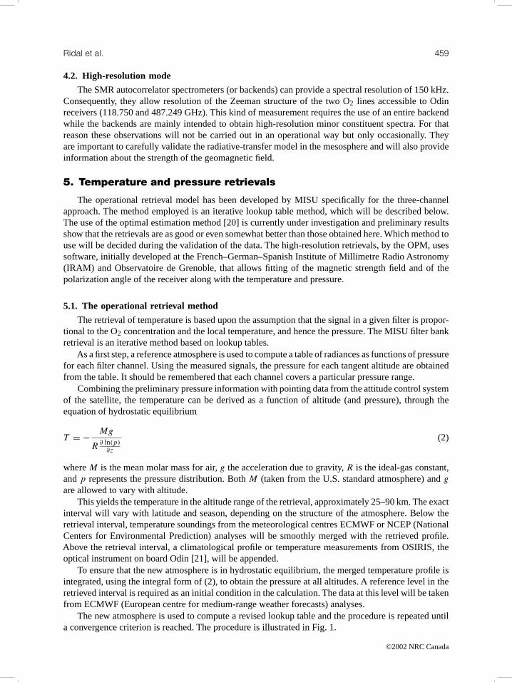
The new atmosphere is used to compute a revised lookup table and the procedure is repeated untila convergence criterion is reached. The procedure is illustrated in Fig. 1.

©2002 NRC Canada

460 Can. J. Phys. Vol. 80, 2002

Fig. 1. The retrieval cycle.

In evaluating (2), we must reduce the sensitivity of the derivative∂ ln(p)/∂z to noise in eitherthe signal or the pointing. The retrieved pressure is therefore smoothed using a running average withGaussian weights. The standard deviation of the Gaussian was choosen to be 3.5 km as a compromisebetween stability and vertical resolution.

5.2. High-resolution retrieval method

The high-resolution retrievals are fitting routines specifically developed to treat the O2 spectroscopicobservations to be performed occasionally using the high-resolution backends. Those observations andtheir special retrievals are aimed at studying the strength of the magnetic field and getting correctvalues of the temperature and O2 mixing ratio above∼65 km. This is possible since the high-resolutionobserving mode (see Sect. 4.2) can resolve the Zeeman components of the O2 emission line.

The high-resolution retrieval software has been developed by the OPM for the French–German–Spanish Institute of Millimetre Radio Astronomy. Among other applications it allows us to fit, in thecase of interest here, the magnetic-field strength and the angle of the polarization of the receiver alongwith the temperature, O2 mixing ratio, and pressure. The retrieval is based upon a generalized nonlinearleast-squares algorithm previously described and used to analyze different sets of atmospheric datain refs. 3, 10, 22, 23, and 24 (the last reference includes retrievals from O2 spectra obtained with aballoon-borne sub-millimetre instrument).

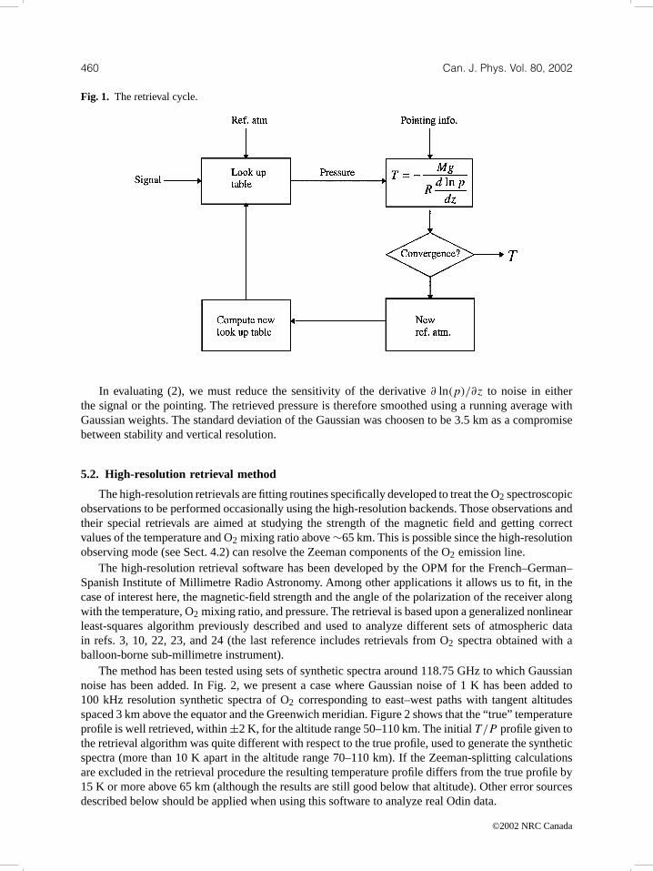
The method has been tested using sets of synthetic spectra around 118.75 GHz to which Gaussiannoise has been added. In Fig. 2, we present a case where Gaussian noise of 1 K has been added to100 kHz resolution synthetic spectra of O2 corresponding to east–west paths with tangent altitudesspaced 3 km above the equator and the Greenwich meridian. Figure 2 shows that the “true” temperatureprofile is well retrieved, within±2 K, for the altitude range 50–110 km. The initialT/P profile given tothe retrieval algorithm was quite different with respect to the true profile, used to generate the syntheticspectra (more than 10 K apart in the altitude range 70–110 km). If the Zeeman-splitting calculationsare excluded in the retrieval procedure the resulting temperature profile differs from the true profile by15 K or more above 65 km (although the results are still good below that altitude). Other error sourcesdescribed below should be applied when using this software to analyze real Odin data.

©2002 NRC Canada

Ridal et al. 461

Fig. 2. Retrieved temperatures from a set of synthetic spectra corresponding to the high-resolution mode. Thespectra on the right show the residual after their fit. Details on generating the synthetic spectra and the retrievalitself are given in Sect. 5.2.

6. Retrieved profiles from the operational mode

A few examples of retrieved temperature profiles using synthetic spectra from the 118.75 GHz line,using the filter bank method are presented here. The simulations include ozone and water vapour, whichhave lines that may disturb this oxygen line. Thermal noise is added to the simulated measurementand the starting profile used to calculate the first reference spectra is a standard temperature profile(indicated in the figures), unless otherwise stated. Vertical sampling of the simulation is 2 km.

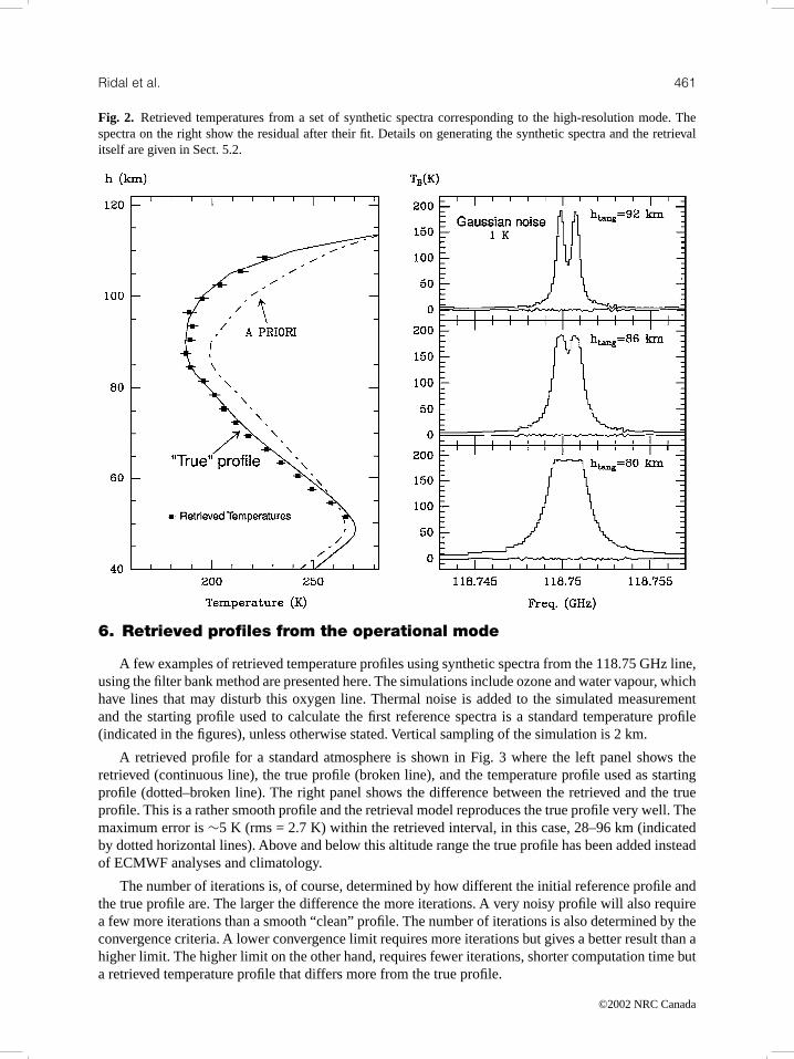
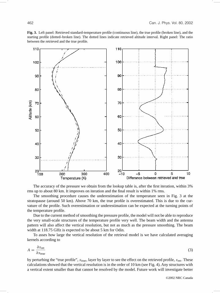
A retrieved profile for a standard atmosphere is shown in Fig. 3 where the left panel shows theretrieved (continuous line), the true profile (broken line), and the temperature profile used as startingprofile (dotted–broken line). The right panel shows the difference between the retrieved and the trueprofile. This is a rather smooth profile and the retrieval model reproduces the true profile very well. Themaximum error is∼5 K (rms = 2.7 K) within the retrieved interval, in this case, 28–96 km (indicatedby dotted horizontal lines). Above and below this altitude range the true profile has been added insteadof ECMWF analyses and climatology.

The number of iterations is, of course, determined by how different the initial reference profile andthe true profile are. The larger the difference the more iterations. A very noisy profile will also requirea few more iterations than a smooth “clean” profile. The number of iterations is also determined by theconvergence criteria. A lower convergence limit requires more iterations but gives a better result than ahigher limit. The higher limit on the other hand, requires fewer iterations, shorter computation time buta retrieved temperature profile that differs more from the true profile.

©2002 NRC Canada

462 Can. J. Phys. Vol. 80, 2002

Fig. 3. Left panel: Retrieved standard-temperature profile (continuous line), the true profile (broken line), and thestarting profile (dotted–broken line). The dotted lines indicate retrieved altitude interval. Right panel: The ratiobetween the retrieved and the true profile.

The accuracy of the pressure we obtain from the lookup table is, after the first iteration, within 3%rms up to about 80 km. It improves on iteration and the final result is within 1% rms.

The smoothing procedure causes the underestimation of the temperature seen in Fig. 3 at thestratopause (around 50 km). Above 70 km, the true profile is overestimated. This is due to the cur-vature of the profile. Such overestimation or underestimation can be expected at the turning points ofthe temperature profile.

Due to the current method of smoothing the pressure profile, the model will not be able to reproducethe very small-scale structures of the temperature profile very well. The beam width and the antennapattern will also affect the vertical resolution, but not as much as the pressure smoothing. The beamwidth at 118.75 GHz is expected to be about 5 km for Odin.

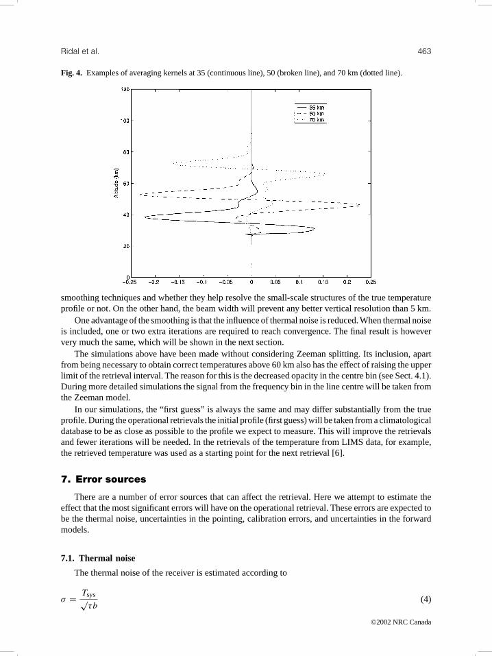
To asses how large the vertical resolution of the retrieval model is we have calculated averagingkernels according to

A = ∂xret

∂xtrue(3)

by perturbing the “true profile”,xtrue, layer by layer to see the effect on the retrieved profile,xret. Thesecalculations showed that the vertical resolution is in the order of 10 km (see Fig. 4). Any structures witha vertical extent smaller than that cannot be resolved by the model. Future work will investigate better

©2002 NRC Canada

Ridal et al. 463

Fig. 4. Examples of averaging kernels at 35 (continuous line), 50 (broken line), and 70 km (dotted line).

smoothing techniques and whether they help resolve the small-scale structures of the true temperatureprofile or not. On the other hand, the beam width will prevent any better vertical resolution than 5 km.

One advantage of the smoothing is that the influence of thermal noise is reduced.When thermal noiseis included, one or two extra iterations are required to reach convergence. The final result is howeververy much the same, which will be shown in the next section.

The simulations above have been made without considering Zeeman splitting. Its inclusion, apartfrom being necessary to obtain correct temperatures above 60 km also has the effect of raising the upperlimit of the retrieval interval. The reason for this is the decreased opacity in the centre bin (see Sect. 4.1).During more detailed simulations the signal from the frequency bin in the line centre will be taken fromthe Zeeman model.

In our simulations, the “first guess” is always the same and may differ substantially from the trueprofile. During the operational retrievals the initial profile (first guess) will be taken from a climatologicaldatabase to be as close as possible to the profile we expect to measure. This will improve the retrievalsand fewer iterations will be needed. In the retrievals of the temperature from LIMS data, for example,the retrieved temperature was used as a starting point for the next retrieval [6].

7. Error sources

There are a number of error sources that can affect the retrieval. Here we attempt to estimate theeffect that the most significant errors will have on the operational retrieval. These errors are expected tobe the thermal noise, uncertainties in the pointing, calibration errors, and uncertainties in the forwardmodels.

7.1. Thermal noise

The thermal noise of the receiver is estimated according to

σ = Tsys√τb

(4)

©2002 NRC Canada

464 Can. J. Phys. Vol. 80, 2002

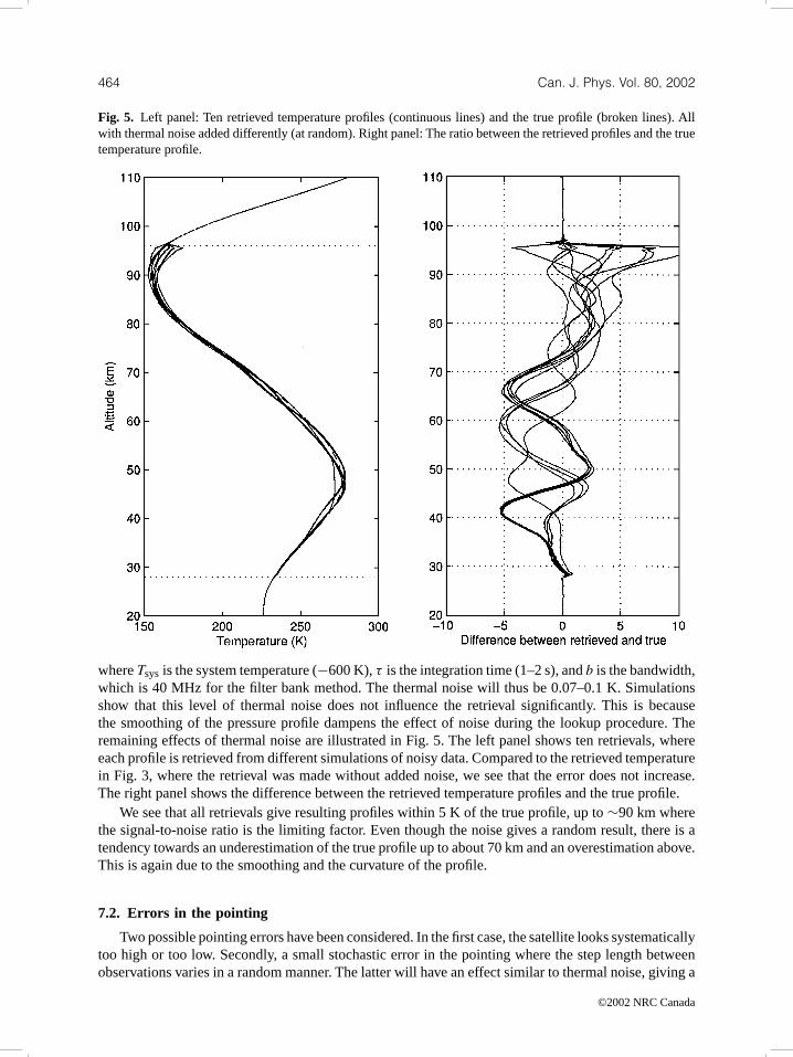
Fig. 5. Left panel: Ten retrieved temperature profiles (continuous lines) and the true profile (broken lines). Allwith thermal noise added differently (at random). Right panel: The ratio between the retrieved profiles and the truetemperature profile.

whereTsysis the system temperature (−600 K),τ is the integration time (1–2 s), andb is the bandwidth,which is 40 MHz for the filter bank method. The thermal noise will thus be 0.07–0.1 K. Simulationsshow that this level of thermal noise does not influence the retrieval significantly. This is becausethe smoothing of the pressure profile dampens the effect of noise during the lookup procedure. Theremaining effects of thermal noise are illustrated in Fig. 5. The left panel shows ten retrievals, whereeach profile is retrieved from different simulations of noisy data. Compared to the retrieved temperaturein Fig. 3, where the retrieval was made without added noise, we see that the error does not increase.The right panel shows the difference between the retrieved temperature profiles and the true profile.

We see that all retrievals give resulting profiles within 5 K of thetrue profile, up to∼90 km wherethe signal-to-noise ratio is the limiting factor. Even though the noise gives a random result, there is atendency towards an underestimation of the true profile up to about 70 km and an overestimation above.This is again due to the smoothing and the curvature of the profile.

7.2. Errors in the pointing

Two possible pointing errors have been considered. In the first case, the satellite looks systematicallytoo high or too low. Secondly, a small stochastic error in the pointing where the step length betweenobservations varies in a random manner. The latter will have an effect similar to thermal noise, giving a

©2002 NRC Canada

Ridal et al. 465

slightly incorrect pressure from the lookup table. The effect is also efficiently damped by the smoothingprocedure.

A small systematic deviation in the pointing, however, will cause a displacement of the retrievedtemperature and pressure profile in altitude. If the deviation is large (more than 3 km) it will be quiteobvious when the profiles from ECMWF are added below 25 km. A 3 km displacement at 25 km, willgive an error in the pressure of about 10 hPa. This is a much larger error than is expected from theretrieval, which is less than 1 hPa (3%) at that altitude.

Odin is expected to have an accuracy in pointing of less than 2 km. Thus, the probability that thepointing error is of the magnitude that will cause problems is rather small.

7.3. Calibration errors

Calibration of the instrument is performed between each atmospheric scan by looking at a hot load onboard the satellite and a cold load (the cosmic background). Both of these are affected by use of internalmirrors so that the telescope is included in the beam path. This could lead to some extra calibrationerrors. However, during the astronomy observations careful calibration against known sources will beused to characterize the telescope.

If the hot-load temperature is either fluctuating or if it is systematically too high (or too low), whilethe temperature of cold space is constant, it will cause an error in the measured brightness temperature.The error will increase with increasing atmospheric temperature. Tests show, however, that this error isexpected to be small, not more than∼0.1 K, i.e., 0.02–0.03% of the measured signal.

To simulate this effect, we reduced the simulated signal at each altitude by 1%, i.e., much more thanexpected. Again we retrieved ten profiles, first without adding thermal noise to see if the calibrationerrors will cause a systematic error, and then with thermal noise included. In the first case, we foundthat the error in the retrieved temperature profile caused by a calibration error of 1% was very small.A systematic structure on the retrieved profile could however be detected. All ten retrieved profiles hadthe same structure. The disturbance was visible between 35–55 km, the region where the temperaturemaximum lies (the stratopause).At this altitude the signal is strongest, and thus the absolute error largest.With thermal noise included in the simulation of the measurement, the result was very similar to theresults in Sect. 7.1. This indicates that the effect of the calibration error is much smaller than that of thethermal noise. If instead of a reduction of the signal, the calibration error should cause a higher signalthan expected, i.e., we add 1% to the simulated signal, the result is similar.

7.4. Errors in the forward model

There are a number of things that may cause errors in the forward-model calculations. A numberof these, such as the angular offset between different radiometers or the antenna response are wellknown for Odin. The astronomy measurements require more detailed specifications of these parametersthan the aeronomy measurements. The spectral parameters, such as the pressure-broadening parame-ters and pressure shift, are hardly a problem since we use very broad filters (40 MHz). However, thespectroscopic-line databases, HITRAN and JPL, will introduce uncertainties that might be significant.

The MISU/CTH model is based on previous model work and compares very well to a similar,independently developed model by the French Odin group [12]. The two models used in this work, theMISU/CTH model and the OPM model, are also in good agreement.

8. Conclusions

By measuring the thermal emission of molecular oxygen in the atmosphere, the Odin satellite willbe able to derive the temperature profile of the atmosphere in two ways. The first is the operationalfilter bank method, which will use thermal emissions from the O2 line at 118.75 GHz. The signal willbe measured in three 40 MHz wide frequency bins and the pressure and temperature profiles will be

©2002 NRC Canada

466 Can. J. Phys. Vol. 80, 2002

retrieved through an iterative process. The second is a high-resolution method with the possibility toobserve both the 118.75 GHz line and the oxygen line at 487.25 GHz. The high-resolution spectra willbe used to get new accurate measurements of the Zeeman-splitting effect. Temperature and pressure canalso be derived from these high-resolution spectra with the retrieval software developed at OPM. Thetemperature and pressure from the high-resolution measurements will be used to validate the operationalretrievals.

Our simulations show that the operational retrieval method is expected to give good results. Atemperature profile can be retrieved to a precision that lies within a root mean square of 3 K, whenthe largest error sources are included. This will meet the requirements from the retrievals of otheratmospheric constituents which use the temperature as input.

The vertical resolution of the retrievals is expected to be around 10 km. The primary reason whythis is not better is the smoothing of the pressure profile obtained from the lookup table. We currentlyuse a Gaussian smoothing but are investigating better methods. Another limiting factor is the antennabeam width. Even though the beam width for Odin is about 5 km most of the information will comefrom the main lobe since the side lobes are very suppressed.

A number of different error sources were tested and shown to be of minor importance unless theyassume unreasonably large values. The two errors that will have any effect on the retrieved profiles arethe thermal noise and errors from the spectroscopic databases.

Acknowledgements

The work by the MISU group has been supported by grants from the Swedish National Space Board.J.R.P. gratefully acknowledges the financial support of the NASA-Goddard Institute for Space Studies,the Observatoire de Paris-Meudon, CNES, and Meteo-France for the development of this work.

References

1. D. Murtagh, U. Frisk, F. Merino et al. Can. J. Phys.80 (2002). This issue.2. J.R. Pardo, M. Ridal, D.P. Murtagh, and J. Cernicharo. Can. J. Phys.80 (2002). This issue.3. J.R. Pardo, L. Pagani, M. Gerin, and C. Prigent. J. Quantum Spectrosc. Radiat. Transfer,54, 931 (1995).4. J.C. Gille and F.B. House. J. Atmos. Sci.28, 1427 (1971).5. J.T. Houghton, F.W. Taylor, and C.D. Rodgers. Remote soundings of atmospheres. Cambridge University

Press, Cambridge, New York. 1984.6. J.C. Gille, J.M. Russel, P.L. Bailey, L.L. Gordely, E.E. Remsberg, J.H. Lienesch, W.G. Planet, F.B.

House, L.V. Lyjak, and S.A. Beek. J. Geophys. Res.89, 5147 (1984).7. E.F. Fishbein, R.E. Cofield, L. Froidevaux et al. J. Geophys. Res.101, 9983 (1996).8. M.E. Hervig, J.M. Russel, L.L. Gordely et al. J. Geophys. Res.101, 10 277 (1996).9. G.K. Hartmann, W. Degenhardt, M.L. Richards et al. Geophys. Res. Lett.23, 2329 (1996).

10. B.J. Sandor and R.T. Clancy. Geophys. Res. Lett.24, 1631. (1997).11. P. Baron, P. Ricaud, J. de la Noë, J.E.P. Eriksson, F. Merino, M. Ridal, and D.P. Murtagh. Can J. Phys.

80 (2002). This issue.12. J.E.P. Eriksson, F. Merino, D. Murtagh, P. Baron, P. Ricaud, and J. de la Noë. Can J. Phys.80 (2002).

This issue.13. H.M. Poynter and D.E. Picket. Appl. Opt.24, 2235 (1985).14. L.S. Rothman, R.R. Gamache, R.H. Tipping et al. J. Quantum Spectrosc. Radiat. Transfer,48, 469

(1992).15. H.J. Liebe, G.A. Hufford, and M.G. Cotton. Proceedings NATO/AGARD Wave Propagation Panel. 52nd

Meeting. 17–20 May 1993, Palma de Mallorca, Spain. 1993. No. 3, pp. 1–10.16. H.J. Liebe. Radio Sci.20, 1069 (1985).17. H.J. Liebe. Int. J. Infrared Millimeter Waves,10, 631 (1989).18. J. Cernicharo. Thése de doctorat d’Etat, Université de Paris VI. 1988.19. P.W. Rosenkranz. J. Quantum Spectrosc. Radiat. Transfer,39, 287 (1988).20. C.D. Rodgers. Rev. Geophys.14, 609 (1976).

©2002 NRC Canada

Ridal et al. 467

21. E.J. Llewellyn, D.A. Degenstein, I.C. McDade et al. Applications of photonic technology-2.Edited byG.A. Lampropoulas and R.A. Lessard. Plenum Press, New York. 1997. pp. 627–632.

22. J.R. Pardo. Thése de doctorate, Université de Paris VI. 1996.23. J.R. Pardo, E. Serabyn, and J. Cernicharo. J. Quantum Spectrosc. Radiat. Transfer,68(4), 419 (2001).24. J.R. Pardo, L. Pagani, G. Olofsson, P. Febvre, and J. Tauber. J. Quantum Spectrosc. Radiat. Transfer,

67(2), 169 (2000).

©2002 NRC Canada