microwave radiation at the u.s. embassy in …
TRANSCRIPT

NTIA-SP-81-12
MICROWAVE RADIATION ATTHE U.S. EMBASSY IN MOSCOW
AND ITS BIOLOGICALIMPLICATIONS: AN ASSESSMENT
PREPARED FOR THEU.S. DEPARTMENT OF STATE
WASHINGTON, D.C. 20520
u.s. DEPARTMENT OF COMMERCEMalcolm Baldrige, Secretary
Dale Hatfield, Acting Assistant Secretaryfor Communications and Information
MARCH 1981
For sale by the Superintendent of Documents, U.S. Government Printing OfficeWashington. D.C. 20402


FORM NTIA·29(.-80)
U.S. DEPARTMENT OF COMMERCENAT·L. TELECOMMUNICATIONS AND INFORMATION ADMINISTRATION
BIBLIOGRAPHIC DATA SHEET
1. PUBLICATION NO. 2. Gov't Accession No. 3, RecIpient's Accession No.
PBS 3 1558044. TITLE AND SUBTITLE
Microwave Radiation at the U.S. Embassy in Moscow andits Biological Implications: An Assessment
M~_~
L'-7~ AUTHOR(S) NTIA/Electromagnetic RadiationAl\dvisory Council(EP~~C); Dept. of State; and Applied Phy~ics Lab.
1
8. PERFORMING ORGANIZATION NAME AND ADDRESS
NTIA/ERMAC, US Dept. of Commerce, Washington, DC 20230;US Dept. of State, Washington, DC 20520; andApplied Physics Laboratory, The Johns Hopkins University
Laurel, Md. 20810.11. Sponsoring Organization Name and Address
US Dept. of StateWashington, DC 20520
"'4. SLIPPLEMENTARY NOTES
S. Publication Date
6, Performing Organization Code
9. ProjecVTask/Work Unit No,
10. ContracVGrant No.
12. Type of Report and Period Covered
13.
1
15, ABSTRACT (A 200-word or less factual summary of most significant information. If document Includes a significant bibliography or literaturesurvey. mention it here.)
,This report presents the results of an assessment of the likelihood of biological·Ieffects from the microwave environment within the U.S. Embassy in Moscow, USSR,based on a retrospective analysis of that environment. It contains a descriptionof the microwave fields and models o~ower density distribution within the Embassyfrom 1966 to 1977; estimated personnel exposures as a function of work and livinglocations in the Embassy; and the results of an assessment of the biological implica~
tions of the type and levels of exposure described. In summary, it was concluded thatno deleterious biological effects to personnel would be anticipated from the microwave exposures as described.
16. Key Words (Alphabet,cal order, separated by semicolons)
~tological effects; biological effects of microwaves; biological effects of nonionizing electromagnetic radiation; Electromagnetic Radiation Management Advisory Council~RMAC; microwaves; Moscow; nonionizing electromagnetic radiation; U.S. Embassy Mosco~
~A';A',lABllIlY51A Te;:.E;:;/"~1E;'~N:::1;---------------T-:1::::8-.-;::Se-c-u-n-:-ty-C~l:-as-s-.";":(T;:';h:-is:-r-e-po:"r-:'t):-----..,..-;2;;;0-.~N::':'u=m:::b::er:-:O::;f·:p:::a~e;--
Jii UNUMITED.
o FOR OFFICIAL DISTRiBUTION.
UncI.
19. Security Class (ThiS page) 21. Price:
Figure 8.
UncI.
N'l'IA Form 29--Bibliogrc.phic Data Sheet.
.. u. S. GOVERNMEfiT PRINTING OFFICI!: 1981 348-727/8480
\


FOREWORD
This report presents the results of an assessment of thelikelihood of biological effects from microwave fields inthe U.S. Embassy in Moscow. In summary, it was concludedthat no deleterious biological effects would be anticipatedfrom the microwave exposures as described in this assessment.
In 1976, press reports on the microwave signals impingingon the U.s. Embassy in Moscow engendered considerablepublic interest and some concerns over the possible biologicaleffects on personnel who had been stationed at the Embassy.
Measurements by the Department of State, showed the powerdensity levels in the Embassy to be extremely low. Theirreviews of medical records and the health of Embassypersonnel did not indicate any problems related to microwaveexposures. Nevertheless, to insure that nothing had beenoverlooked, it was decided to undertake a comprehensiveepidemiological survey of the health status of people whohad been stationed in Moscow between 1953 and 1976. Theresults were compared with those of personnel at otherEastern European posts, not exposed to the microwave signals·This study was conducted by the Department of Epidemiologyat The Johns Hopkins University's School of Hygiene andPublic Health at the request of the Department of State.The results were published by The Johns Hopkins Universityin 1978l!. This study did not show any differences in morbidity or mortality attributable to the presence of microwavesin Moscow. However, the report recommended that -
There is a need for an authoritativebiophysical analysis of the microwavefield that has been illuminating theMoscow Embassy during the past 25 yearswith assessments based on theoreticalconsiderations of the likelihood of anybiological effects.
To satisfy this recommendation the Department of Staterequested the cooperation and assistance of the NationalTelecommunications and Information Administration (NTIA)~t
iiiPreceding Page Blank

The approach adopted was to conduct an analysis of themicrowave fields in the Moscow Embassy followed by anassessment of the likelihood of biological effects.Additional background for this study is available in theAppendix to this report. Results of the assessment of thepotential for biological effects from the microwave fieldsin the Embassy are summarized in Section A. An estimate ofpersonnel exposures as a function of locations within theEmbassy developed by the Department of State is reported inSection B. The results of the retrospective analysis anddescription of the microwave fields in the Embassy by theApplied Physics Laboratory of The Johns Hopkins Universityis contained in Section C.
Notes: 1/ Lilienfe1d, A.M., Tonascia, J., Tonascia, S.,Libauer, C.H., Cauthen, G.M., Markowitz, J.A.,Weida, S., Foreign Service Health Status Study:Evaluation of Health Status of Foreign Serviceand other Employees from Selected EasternEuropean Posts, Department of Epidemiology,of Hygiene and Public Health, The Johns HopkinsUniversity, Baltimore, Maryland 21205. FinalReport, July 31, 1978, 247p. Available fromthe National Technical Information Service (NTIS),5285 Port Royal Road, Springfield, Va. 22161,(703) 487-4650, Accession No. PB 288 163.
'1:../ The National Telecommunications and InformationAdministration (NTIA) is responsible for coordinating Federal Government activities to investigatebiological effects and ensure safe use of microwavesand other radio frequency radiation. It is assistedby the Electromagnetic Radiation Management AdvisoryCouncil (ERMAC) which advises on side effects andthe adequacy of control of such radiations andrecommended a comprehensive Federal program intheir 1971 report.
iv

TABLE OF CONTENTS
PME
FOREWORD iii
SECTION A: ERMAC Assessment of the Potential A-1for Biological Effects fromMicrowave Illumination of the U.S.Embassy in Moscow
SECTION B: A Model of Personnel Exposure B-1
SECTION C: A Model of the Microwave Intensity C-1Distribution within the U.S. Embassyin Moscow, 1966-1977
APPENDIX: Work Statement
v


SECTION A
ERMAC ASSESSMENT OF THE POTENTIAL FORBIOLOGICAL EFFECTS FROM MICROWAVE
ILLUMINATION OF THE U.S. EMBASSY IN MOSCOW
The Electromagnetic Radiation Management Advisory Council(ERMAC) * met on August 26, 1980 to assess the biologicalimplications of the microwave environment within the U.S.Embassy in Moscow, based on a retrospective analysis of thatenvironment. This assessment was undertaken in response to arecommendation in the 1978 "Foreign Service Health Status Study"by The Johns Hopkins University School of Hygiene and PublicHealth which reads as follows:
There is a need for an authoritativebiophysical analysis of the microwavefield that has been illuminating theMoscow Embassy during the past 25 yearswith assessments based on theoreticalconsiderations of the likelihood of anybiological effects.
To implement this recommendation, the Department of Staterequested the assistance of the National Telecommunications andInformation Administration (NTIA). The Johns Hopkins UniversityApplied Physics Laboratory was requested to develop as completea physical description of the U.S. Embassy microwave environmentas possible using all available data. Models were developeddescribing the microwave power density distribution within theEmbassy during the period January 1966 to February 1977. Basedon these models,the Department of State estimated personnelexposure as a function of location in the Embassy. After reviewing this information, the ERMAC was asked to assess the likelihoodof any biological effects from the microwave environment andestimated exposures described.
The Council agreed that the models presented tend to overstaterather than understate the probable microwave levels and that thereis no indication of any significant variations from the modelsover time.
The Council discussed the current state of knowledge andon-going research on biological effects of microwave radiation.A considerable number of scientific investigations have beenconducted and biological effects have been reported from
* Membership and Charter attached.
A-I
January 1981

exposures to power densities higher than those under assessmentand to specific modulation frequencies not found in the Moscowsignals. It was agreed that there is no scientific evidence,nor are there any theoretical grounds to suggest that biologicaleffects would be expected to occur from the type and low levelsof exposure as presented in the models.
Consequently, the ERMAC concluded that no deleteriousbiological effects to personnel would be anticipated from themicrowave exposures at the U.S. Embassy in Moscow as describedin this assessment.

ELECTROMAGNETIC RADIATION MANAGEMENT ADVISORY COUNCIL
MEMBERS
W. Ross Adey, M.D.Associate Chief of Staff
for ResearchJerry L. Pettis Memorial VeteransHospital
11201 Benton StreetLorna Linda, CA 92357
Dr. Mary Ellen O'ConnorAssociate Professor of PsychologyChair, Faculty of Social andBehavior Sciences
University of Tulsa600 S. College AvenueTulsa, OK 74104
Dr. Stephen F. ClearyProfessor of BiophysicsDepartment of BiophysicsMedical College of VirginiaVirginia Commonwealth UniversityRichmond, VA 23298
Dr. Amitai W. EtzioniDirectorCenter for Policy Research199 L Street N.W., Suite 601Washington, D.C. 20036
Mr. Harold Gauper Jr.Electrical EngineerResearch & Development CenterGeneral Electric Company1 River RoadSchenectady, NY 12345
Dr. Arthur W. GuyProfessor & DirectorBioelectromagnetics Research LaboratoryDepartment of Rehabilitation Medicine, RJ-30School of MedicineUniversity of WashingtonSeattle, WA 98195
Dr. William T. Ham Jr.Professor EmeritusDepartment of BiophysicsMedical College of VirginiaVirginia Commonwealth UniverstiyBox 877, MCV StationRichmond, VA 23298
A-3

Ms. H. Janet HealerProgram Manager, Nonionizing RadiationNational Telecommunications and
Information Administration1325 G Street N.W., Suite 250Washington, D.C. 20005
Marylou Ingram, M.D.Director, Institute for Cell AnalysisUniversity of Miami Hospital & Clinic1475 N.W. 12th AvenueMiami, FL 33101
Dr. Samuel KoslovAssistant to the Director for
Technical AssessmentApplied Physics LaboratoryJohns Hopkins UniversityLaurel, MD 20810
Mr. William W. MumfordEngineering Consultant4 Craydon StreetMorris Plains, NJ 07950
Herbert Pollack, M.D., Ph.D.Medical ConsultantProfessor Emeritus Clinical MedicineGeorge Washington University2700 Calvert Street N.W.Washington, D.C. 20008
Mr. George SacherSenior Biologist, Argonne Nat. Lab. (Ret.)926 Chicago AvenueDowners Grove, IL 60515
Dr. Charles SusskindProfessor Engineering ScienceCollege of EngineeringUniversity of CaliforniaBerkeley, CA 94720
Mr. George M. WilkeningHead, Environmental Health
and Safety DepartmentBell LaboratoriesMurray Hill, NJ 07974
A-4

.....
U. S. DEPARTMENT OF COMMERCE
Charter of
ELECTROMAGNETIC RADIATION MANAGEMENT ADVISORY COUNCIL
ESTABLISHMENT
The Electromagnetic Radiation Management Advosory Council (theCouncil) was established on December 11, 1968 and provided adviceto the Director, Office of Telecommunications Management and hissuccessor, the Director, Office of Telecommunications Policy,Executive Office of the President. The majority of the functionsof the latter office (and the Council) were transferred to theDepartment of Commerce by Executive Order 12046 of March 27, 1978and are performed by the National Telecommunications andInformation Administration.
The Secretary of Commerce having determined after consultationwith the General Services Administration that is in the publicinterest in connection with performing duties imposed on theDepartment by and executive order 12046 hereby continues theElectromagnetic Radiation Management Advisory Council pursuantto the Federal Advisory Committee Act, 5 U.S. C. App. (1976).
SOCPE AND OBJECTIVES
The Electromagnetic Radiation Management Advisory Council willadvise the Secretary of Commerce on side effects and the adequacyof control of electromagnetic radiations arising from telecommunications activities. It will review, evaluate, and recommendmeasures to investigate and mitigate potential undesirableeffects on the environment. Its objectives include:
(a) the review of Government and non-Government activitiesbearing upon the adequacy of control of electromagneticapplications which may involve directly or indirectly theproduction of radiant energy in any portion of the spectrumcapable of causing either harmful biological effects, or harmto equipment and material. (The spectrum is presumed toconsist of the electromagnetic spectrum range from electrostaticand constant magnetic fields through the radio frequency to theoptical spectrum, including the use of coherent optical radiation(lasers), and x-rays produced by electrical or electromagneticdevices. )
(b) the review, as required, of matters relating to nonelectromagnetic radiation phenomena (such as infrasonic andultrasonic radiation) which may derive from the use of electronicequipment or be under the purview of those agencies of theGovernment concerned with the electromagnetic spectrum.
A-S

The Council will function solely as an advisory body, in accordancewith the provisions of the Federal Advisory Committee Act.
MEMBERS AND CHAIRPERSON
(a) The Council shall consist of no more than fifteen members, asneeded, to be appointed by the Assistant Secretary for Communicationsand Information to assure a balanced representation in such areas asengineering, the physical sciences, biomedical and the healthsciences. The members will be appointed for a period of two yearsand will serve at the discretion of the Assistant Secretary. Vacancyappoints shall be for the remainder of the unexpired term of thevacancy.
(b) The Chairperson of the Council is the Assistant Secretary forCommunications and Information or designee.
ADMINISTRATIVE PROVISIONS
(a) The Council will report to the Secretary through the AssistantSecretary for Communications and Information.
(b) Members of the Council will not be compensated for theirservices but will, upon request, be allowed travel expenses incurredin the performance of their duties, as authorized by5 U.S.C. 5701et. seq.
(c) Administrative support for its activities will be provided bythe National Telecommunications and Information Administration and isestimated not to exceed $25,000 annually which includes one-fourthperson year of effort.
(d) Meetings will be held at approximately three-month intervals atthe call, or with the approval of the responsible Departmentalofficial or his representative, and with an agenda formulated andapproved by such official. No meeting shall be conducted in theabsence of this official.
(e) Detailed minutes of each meeting shall be kept and shall containa record of the persons present, a complete and accurate descriptionof matters discussed and conclusions reached, and copies of allreports received, issued or approved by the Council. The accuracy ofall minutes shall be certified to by the Chairperson of the Council.
A-6
,..

DURATION
~he Electro~a9netic Radiation Management Advisory Councilahall·terminate two years from the date of this charter unlessterminated earlier or renewed by proper authority by appropriateaction.
9 "tAN 1981
Date
Pursuant to subsection 9(c) of the Federal Advisory CommitteeAct,S U.S.C. App. (1976), this committee was filed with theAssistant Secretary for Administration on January 9, 1981. Onthe same date, copies were filed with the following committees ofCongress, and a copy furnished the Library of Congress:
Senate Committee on Commerce, Science, and TransportationBouse Committee on Energy and Commerce
~. I~, IfIIC' Date
A-7
SECTION B
A M:lDEL OF PERSONNEL EXPOSURE
Office of Medical ServicesU.S. Department of State
Introduction
One of the recommendations of the Johns Hopkins' Foreign ServiceHealth Status Study was "There is a need for an authoritative biophysicalanalysis of the microwave field that has been illwninating the MoscowEmbassy during the past 25 years with assessments based on theoreticalconsiderations of the likelihood of any biological effects."
The Department of State requested the help of NTIA in carrying outthis recommendation. It was planned that the overall approach wouldconsist of three phases: Phase I, as complete a physical description ofthe Moscow field as possible; Phase II, estimation of exposure for modelpersonnel and Phase III, assessment of the likelihood of any biologicaleffects.
Accordingly the Applied Physics Laboratory (APL) of the Johns HopkinsUniversity (JHU) was asked to carry out Phase I. The docwnent entitled"A M:lDEL OF THE MICROWAVE INTENSITY DISTRIBUTION WITHIN THE U.S. EMBASSY,MJSCOW 1966 to 1977" prepared by Robert C. Malla1ieu of the APL is adescription and summary of this phase.
Background
The illwnination of the Chancery can be divided into two periods. Thefirst code name TUMS, from 1953 to 26 May 1975, and the second, code nameMUTS from 28 May 1975 until February 1977. The MUTS interval is divided intotwo parts by the installation of window screens on February 5, 1976. Thefirst MTUS interval extends from 28 May 1975 to 5 February 1976 and the secondinterval, in which the fields were reduced due to both the screening andreductions in transmitter power, extends from 6 February 1976 until 1 February1977. In 1962 the Department of State instituted a system for continuouslymonitoring the signals using strip-chart recorders. Power density and frequencymeasurements also were made but records of actual power density measurementsprior to 1966 were not adequate for analysis so that the models of themicrowave intensity distribution within the Embassy extend only from January1966 to February 1977.
For the TUMS period the power density was measured directly. Duringthe MUTS interval the electric-field energy density was measured and the"equivalent" power density calculated.
The APL report was careful to point out "that power density 'values'alone are not sufficient to describe the microwave fields with the Chancery."It is acknowledged that even at the same point in such an envirornnent, thepower density as measured by these two methods will differ and so will theelectric (E) and magnetic (H) field strengths inferred from the measurements.The "equivalent" power density will be higher if read at an electric-fieldantinode, but the inferred higher E and H fields are not simultaneous andcollocated. The direct power density is lower, but its lower E and H fieldsare oriented to allow a relatively more efficient transfer of power.
B-1 August 1980

TUMS (Technically Unidentified Moscow Signal)
During the TUMS period there was a single source of the microwavebeam from a Soviet apartment house about 100 meters west of the Chancery.The west facade of the central building waS illuminated. The highestintensities appeared between the 3rd and 9th floors with lower levels onthe 1st. 2nd. and 10th. Only rooms with windows or doors on this westwall were directly affected (although the model assigns lower power densityvalues to interior rooms. no measurable levels were recorded there). Thehighest levels were within 2 feet of doors and windows on the west wall.The severe winter weather (as low as 45° F and C below zero) usually resulted in placing the desks away from the window areas in the workingrooms on the 7th. 8th and 9th floors. The average power densitY* throughout illuminated exterior rooms. at greater distances from the windows.was about 1. 5 microwatts / cm2 •
In the living quarters from the 3rd to the 7th floors. the kitchensand main bedrooms had windows in the west wall. The layout of thekitchens. which were about 7 feet wide and 18 feet long put the refrigeratoron the west wall just north of the window. When the door was opened itserved as a screen across the window. so that anyone taking out or putting foods into the refrigerator was shielded from the microwaves comingthrough the window. The stove and the sink were about 4 feet from thewindow. the stove on the south wall and the sink on the north wall. Theclothes washer was at least 10 feet from the window. The layout in thebedroom usually showed the headboards against the south wall at least4 feet from the west wall (again this was protection from the cold drafts).The average figure of 1.5 microwatts/cm2 may be applied to these illuminated rooms. Living rooms and dining areas and bathrooms werenot exposed in the TUMS period.
MUTS (Moscow Unidentified Technical Signal)
For the MUTS episode the transmission originated from two sources.one the roof of an apartment house about 100 meters east of the Chancery.and the other an office building about the same distance south. Many windows were facing east in the central building. but only two rooms. 901 and1001 and two south stairway areas on the 8th and 9th floors had windowsfacing south.
Screening was installed by 6 February 1976 and that. along with aseries of transmitter power reductions. reduced the levels within thebuildings to "less than 0.1 microwatts/cm2". That figure serves for thesecond portion of the MUTS model.
*The average power density levels throughout the illuminated rooms canbe assumed to be half the working area antinode values.
B-2

Prior to the screening~ the highest levels were recorded in the officeson the east side of the central building with increasing intensities towardthe southeast rooftop corner (above Room 1001). The average antinodeequivalent power density was as high as 10.2 microwatts/cm2 within 2 feetof the window in Room 1003 although the average antinode level in the working area of the room was only 3.0 microwatts/ cm2. Room 901 had an average antinode level of 9.0 microwatts / cm2 through much of the room in July1975 although the average was less than 2 microwatts/cm2 when data takingresumed in November 1975. These few values were the highest sustainedor repeated levels. Inside the building~ the highest reading was 24 microwatts / cm2 within 2 feet of the window in room 1001 during a two hour periodof unusual signal strength on 24 January 1976.
Typically~ the levels even on the top floors of the central building werelower. On these upper floors~ the average antinode within 2 feet of thewindows was 3.3 microwatts/ cm2; further within the rooms~ the averageantinode level was 2.2 microwatts/cm2. The average power density awayfrom the windows would have been about 1. 5 microwatts / cm2. Again~ onlythe rooms with windows on the east facade were involved. Within the livingquarters in the central building and the north and south wings~ only oneapartment has an average antinode level above 1.3 microwatts/cm2 (Apartment 7B in the south wing had a level of 1. 6 microwatts / cm2). The averagepower density throughout this apartment would have been about half of theantinode level or about 0.8 microwatts/cm2.
Summary of Typical Exposures for Model Personnel
A close approximation can be made of the actual number of peopleworking or living in the various designated regions at the specific times.Over the period of time from 1953 to 1976 there were 1827 employeeswhose tours of duty were usually two years. A few served only one year.Several extended for two and even three tours. Over the same time therewere about 3000 dependents.
During the TUMS period State Department employees in working areaswith an average power density of about 1.5 microwatts/cm2 at any giventime numbered:
West 8th floor --209th floor - - 2
Over the period of 22 years it is estimated that there were about 240employees exposed to an average power density of about 1.5 microwatts/ cm2for approximately 2 hours during the workday (8 a. m. to 5 p. m.). Duringweekdays (Monday to Friday) the exposed working areas were illuminatedfor a maximum of 6 hours during each 24 hour period.
B-3

It is difficult to estimate how many people who worked on the 8thand 9th floors also lived in the central wing. However. the few who didreceived an additional average exposure of about 1. 5 microwatts / cm2 for3 hours a day during the two day weekend.
As to the dependents there were 15 apartments on the 3rd through 7thfloors large enough to house several children (an average of 4 in the family).During the TUMS period this group was possibly exposed to an average ofabout 1.5 microwatts/cm2 (about 660 people over the 22 years). There were4 smaller double apartments housing about 2 in each or 8 people at a time.These were in region 2 calculated as receiving about 0.75 microwatts/cm2.In the south wing there were 6 apartments occupied by singles. These 6people were exposed to less than 0.1 microwatts/cm2. During weekdays theabove apartments were illuminated for a maximum of 6 hours during each24 hour period and for 3 hours a day during the two day weekend.
The MUTS episode lasted only about eight months. During this timethere were about 26 employees involved. These employees with few exceptions were exposed to an average power density of about 1. 5 microwatts/ cm2 for 4 to 8 hours during the workday. During weekdays theexposed working areas were illuminated for a maximum of II to 16 hoursduring each 24 hour period.
The exceptions noted above were those who worked in a few offices onthe upper floors of the central building (Rooms 701. 802. 804. 901. 1001 and1002). Antinode levels in those rooms may be found from Table 4. summarizing data from the two MUTS surveys. The average levels in each roomwould have been about half of the antinode values.
During the MUTS period the microwave beam was focused more sharplyon the upper floors. Within the living quarters in the central building andthe north and south wings. the highest average power density value in illuminated rooms was about 0.8 microwatts/cm2.
B-4

*SUMMARY OF TRANSMITTER OPERATING (RECORDED) TIME
TRANSMITTER TIME INTERVAL TIME PERIODS 0/0 OF TIME ON
TUMS 2/1/66 to morning (midnight 22 (1. 8 hrs.)to 8 am)
12/31/70 workday (8 am-5 pm) 23 (2.1 hrs. )evening (5 pm to 20 (1.4 hrs. )
midnight)
weekdays 25 (6 hrs.)weekend days 12 (3 hrs.)
summer (JJAS) days 25 (6 hrs.)other than summer 20 (4.8 hrs.)
days
MUTS-l 7/1/75 to morning 35 (2.8 hrs.)10/15/75 workday 44 (4.0 hrs.)
evening 45 (3.2 hrs.)
weekdays 45 (11 hrs.)weekend days 31 (7.5 hrs)
MUTS-l & 10/16/75 to morning 47 (4.0 hrs.)MUTS 2 2/5/76 workday 83 (7.5 hrs.)
evening 56 (3.9 hrs.)
weekdays 65 (15.6 hrs.)weekend days 58 (13.9 hrs.)
POST SCREENING 2/6/76 to morning 26 (2.1 hrs.)3/4/76 workday 73 (6.6 hrs.)
evening 26 (1.8 hrs. )
weekdays 50 (12 hrs.)weekend days 30 (7.2 hrs.)
* Based on data in Johns Hopkins Applied Physics LaboratoryReport, Appendix E (Summary Time Charts of TransmitterOperating Hours.)
B-SAttachment I

~
tl1 I 0'\
F: f rt H H
Tab
le1
TUM
Sm
icro
wav
epo
wer
den
sity
mod
el.
Pow
erd
ensi
ty(v
W/c
m2 )
Reg
ion
·Ant
inod
ew
ith
inA
nti
no
de
else
wh
ere
Ave
rage
thro
ug
ho
ut
Tra
nsi
ent
du
rin
gn
o.
Des
crip
tio
no
fre
gio
n2
fto
fw
indo
win
the
room
the
room
mod
ech
ang
es
1C
entr
alb
uil
din
gro
oms
and
stai
rway
sad
ja-
42
.51
.520
(last
ing
be-
cen
tto
the
wes
tw
all
of
the
bu
ild
ing
that
twee
n10
seco
nd
sha
vea
win
dow
or
do
or
onth
ew
est
wall
.ar
.d2
min
ute
s)th
ird
ton
inth
flo
ors
.in
clu
siv
e(t
he
re-
gio
nw
ith
the
hig
hes
tpo
wer
den
sity
)
2C
entr
alb
uil
din
gro
oms
and
stai
rway
sas
21
.30
.81
0(l
ast
ing
be-
des
crib
edin
Reg
ion
1.
bu
ton
the
firs
t.tw
een
10
seco
nd
sse
con
d,
and
ten
thfl
oo
rs;
any
base
men
tan
d2
min
ute
s)ro
oms
inth
ecen
tral
bu
ild
ing
wit
ha
win
-do
wab
ove
grou
ndle
vel
onth
ew
est
wal
l;ap
arm
ent
room
so
ver
the
no
rth
and
sou
thco
urt
yar
den
tran
ces
wit
ha
win
dow
or
door
onth
ew
est
wal
l;ro
oft
op
so
fall
thre
eb
uil
din
gs
3A
llo
therunshieJ~ed
room
san
dar~as
less
than
less
than
less
than
less
than
abov
egr
ound
lev
el
inall
thre
eb
uil
d-
0.1
0.1
0.1
0.1
ing
s
4A
llsh
ield
edro
oms;
all
room
sbe
low
Too
low
toT
oolo
wto
Too
low
toT
oolo
wto
grou
ndle
vel
inall
~hree
bu
ild
ing
ses
tim
ate
esti
mat
ees
tim
ate
est
imate
wit
hno
wes
tw
indo
w
~ "...
C:z
:m
m°5
>,,
:z:
cZ
z:D
-(cn
~ClJx
.~(;
j~(J)z
e>~
zm
z°O~
::0:1
1~fS
0-< ~

THE JOHNS HOPKINS UNIVERSITY
APPLIED PHYSICS LABORATORYLAUREL, MARYLAND
Table 2
First MUTS survey (24 to 31 July 1975).
Equivalent plane-wave2power <!ensity (IlW/ cm )
Near closed Work ResonantRoom window area zone Comments
701 3.9 3.9 4.8 Note 1702 3.6 2.1 Note 2703 Negligible704 3.1 2.7 4.2705 3.6 2.7 3.9706 2.7 3.0 Note 2707 3.9 2.6 Note 2708 3.6 3.0 Note 2709 Negligible801 2.1 1.2 3.9802 7.8 3.0 7.2803a 4.8 1.2 8.4 Note 3803b 3.6 3.6 -804 4.5 3.0 -805 3.0 1.5 -806 3.9 1.5 -807 4.2 1.2 -808 2.4 2.4 -809 1.5 1.5 3.9901 6.6 9.0 9.0 Note 4902 3.3 2.4 6.6903 3.0 1.5 4.8904 2.4 1.8 -905 - - 4.2
1001 8.7 4.5 8.71002 8.4 6.9 8.71003 10.2 3.0 9.61004 Negligible1005 Negligible1006 2.7 1.0 Note 21007 - 1.2 -1008 2.4 1.0 - Note 5
Notes:
1. For this table, rooms are numbered from south to north accordingto unnumbered layouts in Ref. 15.
2. Not significantly higher than the work area value.
3. Two entries were made for the room. Entry a is on the sou,thsideand b on the north side.
4.
5.
2In Room 901, the 9.0 IlW/cm power density existed throughout mostof the work area.
2Reference 49 mentions a rooftop power density of 24 IlW/cm and a2reading on an eighth floor balcony of 13.2 IlW/cm contained in
"associated working papers" for this survey. These were the highestreadings obtained during this first survey.
Table entries are the mean of all readings for the most intenseelectric-field antinode found at each location.
B-7
Attachment III

THE JOHNS HOPKINS UNIVERSITY
APPLIED PHYSICS LABORATORYLAUREL, MARYLAND
Table 3
Second MUTS survey (30 November 1975 to 5 February 1976).
Equivalent plane-wave power density (~W/cm2)
Near Throughoutclosed window working area
Number of Standard Date of Standard Date ofRoom measurements Mean deviation Extreme Extreme Mean deviation Extreme extreme Co...ent.
701 2 1.4 - 1.5 13 Dec 1.1 - 1.2 5 Dec702 2 1.8 - 2.4 14 Dec 1.4 - 1.8 14 Dec703 1 0.3 5 Dec704 3 1.5 0.8 2.4 14 Dec 0.9 0.3 1.2 14 Dec705 1 0.9 5 Dec 0.6 5 Dec707 1 0.6 5 Dec 0.6 5 Dec709 1 1.8 1 Dec 1.2 1 Dec801 5 3.4 1.2 5.4 3 Dec 1.3 1.3 3.0 24 Jan802 5 4.6 3.1 9.6 5 Dec 3.3 2.2 6.0 24 Jan803 3 3.5 1.8 4.8 3 Dec 1.0 0.7 1.8 3 Dec804 1 4.8 24 Jan 6.0 24 Jan805 3 2.4 0.6 3.0 30 Nov 1.5 1.1 2.4 30 Nov806 3 2.6 0.4 3.0 3 Dec 1.2 0 1.2807 5 2.4 0.6 3.0 3 Dec 1.3 1.0 2.4 24 Jan808 1 2.4 24 Jan 1.8 24 Jan809 4 1.6 0.6 2.4 24 Jan 1.1 0.9 2.4 24 Jan810 1 1.8 24 Jan 1.2 24 Jan
SS-8 6 0.8 0.4 1.2 1 Dec 0.8 - 1.2 6 Dec901-East 93 2.7 1.8 7.8 4 Dec Rm 901 readinga merged below901-South 49 0.8 0.6 4.2 5 Dec 1.5 1.2 6.0 4 Dec
902 65 2.0 1.5 7.2 24 Jan 2.2 2.0 10.2 24 Jan Nota 1903 32 2.0 1.0 4.0 24 Jan 1.8 1.3 7.2 24 Jan904 5 2.0 1.5 4.2 3 Dec 1.0 1.2 3.0 3 Dec
SS-9 6 2.7 1.3 4.2 16 Jan 1.2 0 1.21001 38 7.2 5.1 24.0 24 Jan 3.7 2.1 8.4 31 Dec1002 31 4.4 2.5 12.0 24 Jan 3.4 2.5 13.2 24 Jan1003 35 Note 2 3.0 2.2 11.4 24 Jan1005 3 1.4 0.9 2.4 10 Dec 0.9 0.8 1.8 10 Dec1006 15 2.0 1.1 3.6 3 Dec 1.1 0.5 1.8 24 Jan1007 1 0.6 5 Dec 1.2 Note 3 5 Dec1008 17 1.8 1.2 4.2 4 Dec 1.7 1.3 3.6 4 DecC5EL 2 0.6 - 0.9 15 DecS5CB 1 0.6 15 Dec 1.2 Note 4 15 DecS5eT, 2 0.5 - 0.6 11 Dec 0.3S5CR 1 0.6 11 Dec 0.3 11 DecS6BK 3 0.7 0.2 0.9 15 Dec 0.9 0.9 1.5 15 DecS6BL 5 0.3 0.4 0.9 8 Dec 0.6 0.6 1.2 15 DecS6BB 3 0.8 0.2 0.9 15 Dec 0.6 0.5 1.2 15 DecS7AL 2 0 0S7BK 2 1.5 - 1.8 15 Dec 1.5 - 2.1 15 DecS7BB 2 1.4 - 1.5 15 Dec 1.6 - 2.1 15 DecS7BL 3 0.8 0.4 1.2 8 Dec 0.3NWR 1 Note 5 3.0 9 DecCWR 1 Note 5 13.2 to 9 Dec
15.0
Notes:
1. Many extreme valuea were recorded on 24 January 1976 during a period of HUTS-lA tranamiaaiona (0.5 to 2 GHz)between 4 and 6 pm (maximum power was at 1.56 GHz).
2. Window area meaaurements ranged aa high as 42.0 ~W/cm2 due to a standing wave from the back of a aafe whichpartially blocks the window; this is not a work area.
3. Readings quoted aa "low" were aasumed to be O. 3 ~W/cm2, as per Ref. 34.
4. Apartment rooma deaignated in Ref. 50 as "room number called S6BB, S6BL, S6BK, 5788, S7BL, S7BK, and S7ALrefer to south wing apa~tments. S6BB is the bedroom in Aparment 6B; S6BL is the living room of Apartment 6B;SCBK is the kitchen of Aparment 6B, etc." SS-8 and SS-9 refer to the southernmost stairways in the centralbuilding on the eighth and ninth floors.
5. For readings on the north wing roof (NWR) and the central wing roof (CWR), measurements were made as close tothe front of the building and as far south as practical.
Table entries are the mean of all readings for the most intense electric-field antinode found at each location.
B-8 AttaChment rv
THE JOHNS HOPKINS UNIVERSITY
APPLIED PHYSICS LABORATORYLAUREL. MARYLAND
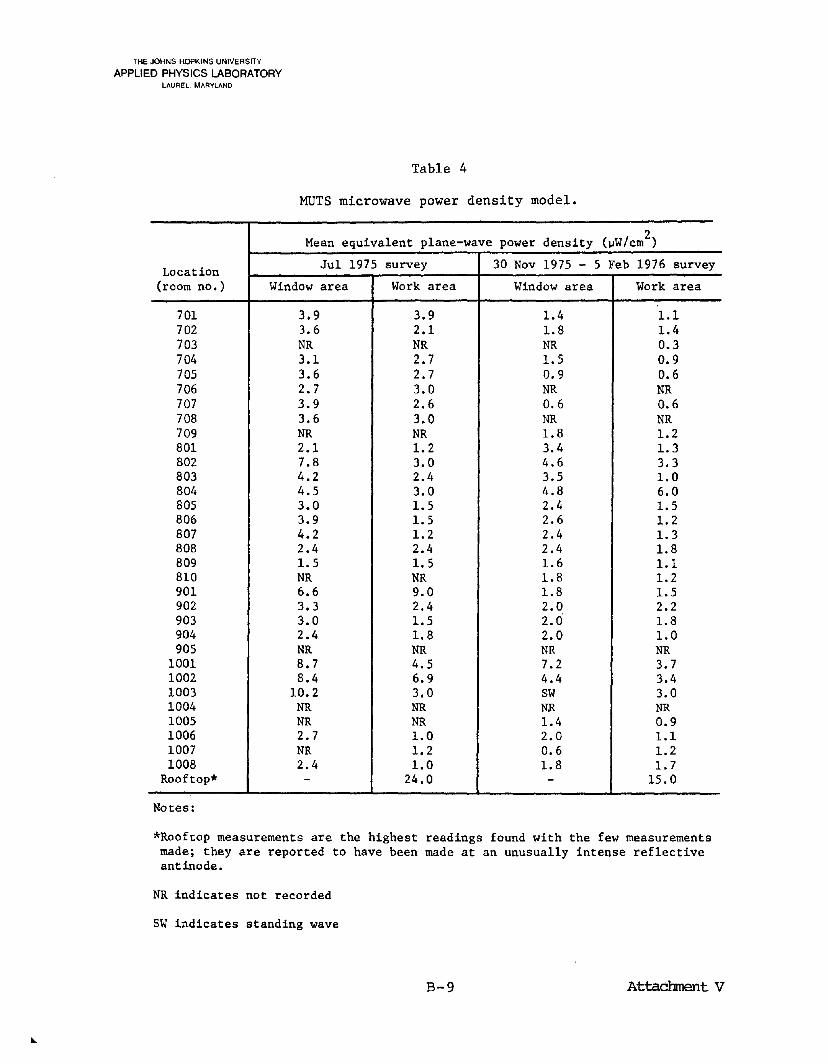
Table 4
MUTS microwave power density model.
2Mean equivalent plane-wave power density (~W/cm )
Location Ju1 1975 survey 30 Nov 1975 - 5 Feb 1976 survey
(room no.) Window area Work area Window area Work area
701 3.9 3.9 1.4 1.1702 3.6 2.1 1.8 1.4703 NR NR NR 0.3704 3.1 2.7 1.5 0.9705 3.6 2.7 0.9 0.6706 2.7 3.0 NR NR707 3.9 2.6 0.6 0.6708 3.6 3.0 NR NR709 NR NR 1.8 1.2801 2.1 1.2 3.4 1.3802 7.8 3.0 4.6 3.3803 4.2 2.4 3.5 1.0804 4.5 3.0 4.8 6.0805 3.0 1.5 2.4 1.5806 3.9 1.5 2.6 1.2807 4.2 1.2 2.4 1.3808 2.4 2.4 2.4 1.8809 1.5 1.5 1.6 1.1810 NR NR 1.8 1.2901 6.6 9.0 1.8 1.5902 3.3 2.4 2.0 2.2903 3.0 1.5 2.0 1.8904 2.4 1.8 2.0 1.0905 NR NR NR NR
1001 8.7 4.5 7.2 3.71002 8.4 6.9 4.4 3.41003 10.2 3.0 SW 3.01004 NR NR NR NR1005 NR NR 1.4 0.91006 2.7 1.0 2.0 1.11007 NR 1.2 0.6 1.21008 2.4 1.0 1.8 1.7
Rooftop* - 24.0 - 15.0
Notes:
*Rooftop measurements are the highest readings found with the few measurementsmade; they are reported to have been made at an unusually intense reflectiveantinode.
NR indicates not recorded
SW indicates standing wave
B-9 Attachment V
...
txl I I-'
o
:J::I
rt rt 11l o § CD ~ rt < H
RO
OF
TO
P*
24.0
1001
1002
1003
1004
1005
1006
1007
1008
8.7
8.4
10.2
NRNR
2.7
NR2.
4
901
902
903
904
905
6.6
3.3
3.0
2.4
NR
801
802
803
804
805
806
807
808
809
810
2.1
7.8
4.2
4.5
3.0
3.9
4.2
2.4
1.5
NR
701
702
703
704
705
706
707
708
709
3.9
3.6
NR
3.1
3.6
2.7
3.9
3.6
NR
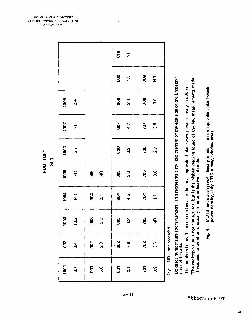
Key
:N
R-
no
tre
cord
ed
Bol
dfac
enu
mbe
rsar
ero
omnu
mbe
rs.
Thi
sre
pres
ents
ast
yliz
eddi
agra
mo
fth
eea
stsi
deo
fth
eE
mba
ssy;
itis
not
tosc
ale.
The
num
bers
belo
wth
ero
omnu
mbe
rsar
eth
em
ean
equi
vale
ntpl
ane-
wav
epo
wer
dens
ity
inpW
/cm
2.
*The
roof
top
valu
eis
no
tth
eav
erag
e,b
ut
isth
ehi
ghes
tre
adin
gfo
und
of
the
few
mea
sure
men
tsm
ade;
itw
assa
idto
beat
anun
usua
lly
inte
nse
refl
ecti
vean
tino
de.
Fig
.4M
UTS
mic
row
ave
pow
erde
nsity
mod
el-
mea
neq
uiva
lent
plan
e-w
ave
pow
erde
nsity
,Ju
ly19
75su
rvey
,w
indo
war
eas.
~ "'0
....cff
im
...0
0"'O~
:I:"
,
~~
02
Scn
z '"~~
00
o
rii
:Dill
a~
~

,.
ttl I I-'
I-'
~ rt rt PJ () § (I)~ rt <: H H
RO
OF
TO
P*
24.0
1001
1002
1003
1004
1005
1006
1007
1008
4.5
6.9
3.0
NRNR
1.0
1.2
1.0
901
902
903
904
905
9.0
2.4
1.5
1.8
NR
801
802
803
804
805
806
807
808
809
810
1.2
3.0
2.4
3.0
1.5
1.5
1.2
2.4
1.5
NR
701
702
703
704
705
706
707
708
709
3.9
2.1
NR2.
72.
73.
02.
63.
0N
R
Key
:N
R-
not
reco
rded
Bol
dfac
enu
mbe
rsar
ero
omnu
mbe
rs.
Thi
sre
pres
ents
ast
yliz
eddi
agra
mo
fth
eea
stsi
deo
fth
eE
mba
ssy;
itis
no
tto
scal
e.T
henu
mbe
rsbe
low
the
room
num
bers
are
the
mea
neq
uiva
lent
plan
e-w
ave
pow
erde
nsit
yin
JlW
/cm
2.
*The
roof
top
valu
eis
no
tth
eav
erag
e;b
ut
isth
ehi
ghes
tre
adin
gfo
und
of
the
few
mea
sure
men
tsm
ade;
itw
assa
idto
beat
anun
usua
lly
inte
nse
refl
ecti
vean
tino
de.
Fig.
5M
UTS
mic
row
ave
pow
erde
nsity
mod
el-
mea
neq
uiva
lent
plan
e-w
ave
pow
erde
nsity
,Ju
ly19
75su
rvey
,w
ork
area
s.
~ -0...
cff
i~5
r-o
J:1::J:~
"'-<
J:~~~
~()~
~cn~
~s:c:
zlX
l'i:
°o
iii:D
el~~
o ~

...
ttl I I-'
l\J
~ rt rt III () § CD ::s rt <: H H H
RO
OF
TO
P*
15.0
1001
1002
1003
1004
1005
1006
1007
1008
7.2
4.4
SWNR
1.4
2.0
0.6
1.8
901
902
903
904
905
1.8
2.0
2.0
2.0
NR
801
802
803
804
805
806
807
808
809
810
3.4
4.6
3.5
4.8
2.4
2.6
2.4
2.4
1.6
1.8
701
702
703
704
705
706
707
708
709
1.4
1.8
NR1.
50.
9NR
0.6
NR1.
8
Key
:N
R-
no
tre
cord
ed,
SW-
stan
ding
wav
e
Bol
dfac
enu
mbe
rsar
ero
omnu
mbe
rs.
Thi
sre
pres
ents
ast
yliz
eddi
agra
mo
fth
eea
stsi
deo
fth
eE
mba
ssy;
itis
no
tto
scal
e.
The
num
bers
belo
wth
ero
omnu
mbe
rsar
eth
em
ean
equi
vale
ntpl
ane-
wav
epo
wer
dens
ity
inj1
W/c
m2
.
*The
roo
fto
pva
lue
isn
ot
the
aver
age,
bu
tis
the
high
est
read
ing
foun
do
fth
efe
wm
easu
rem
ents
mad
e;it
was
said
tobe
atan
unus
uall
yin
tens
ere
flec
tive
anti
node
.
Fig.
6M
UTS
mic
row
ave
pow
erde
nsity
mod
el-
mea
neq
uiva
lent
plan
e-w
ave
pow
erde
nsity
,30
Nov
embe
r19
75to
5Fe
brua
ry19
76su
rvey
,w
indo
war
eas.
~ "....
Cffi
me.
.C
o,,:I:
::I:
~~:
I:-!
il()~
C/l
z
>~
~~
:o~
~~
o ~

,.
ttl I ..... W
~ rt rt III () [ CD ::s rt H X
RO
OF
TO
P*
15.0
1001
1002
1003
1004
1005
1006
1007
1008
3.7
3.4
3.0
NR
0.9
1.1
1.2
1.7
901
902
903
904
905
1.5
2.2
1.8
1.0
NR
801
802
803
804
805
806
807
808
809
810
1.3
3.3
1.0
6.0
1.5
1.2
1.3
1.8
1.1
1.2
701
702
703
704
705
706
707
708
709
1.1
1.4
0.3
0.9
0.6
NR
0.6
NR
1.2
Key
:N
R-
no
tre
cord
ed
Bol
dfac
enu
mbe
rsar
ero
omnu
mbe
rs.
Thi
sre
pres
ents
ast
yliz
eddi
agra
mof
the
east
side
of
the
Em
bass
y;it
isn
ot
tosc
ale.
The
num
bers
belo
wth
ero
omnu
mbe
rsar
eth
em
ean
equi
vale
ntpl
ane-
wav
epo
wer
dens
ity
inJl
W/c
m2
.
*The
roof
top
valu
eis
no
tth
eav
erag
e,b
ut
isth
ehi
ghes
tre
adin
gfo
und
of
the
few
mea
sure
men
tsm
ade;
itw
assa
idto
beat
anun
usua
lly
inte
nse
refl
ecti
vean
tino
de.
Fig.
7M
UTS
mic
row
ave
pow
erde
nsity
mod
el-
mea
neq
uiva
lent
plan
e-w
ave
pow
erde
nsity
,30
Nov
embe
r19
75to
5Fe
brua
ry19
76su
rvey
,w
ork
area
s.
~ "lJ
....cff
i~1
5r-"lJ~
l::I
:tb
"-(x
f!!~~
3:(')~
~cn~
~s;:
~ze
D:;
::°O
m JJill
a~
~

SECTION C
FS-80-166AUGUST 1980
A MODEL OF THE MICROWAVEINTENSITY DISTRIBUTION WITHINTHE US EMBASSY IN MOSCOW,1966 to 1977
R. C. MALLALIEU
FLEET SYSTEMS DEPARTMENT
THE JOHNS HOPKINS UNIVERSITY. APPLIED PHYSICS LABORATORYJohns Hopkins Road, Laurel, Maryland 20810Operating under Contract N00024·78·C·5384 with the Department of the Navy


THE JOHNS HOPKINS UNIVERSITY
APPLIED PHYSICS LABORATORYLAUREL, MARYLAND
CONTENTS
1.
2.
3.
4.
5.
6.
A.
B.
C.
D.
E.
List of Illustrations
List of Tables •
Sununary
Power Density and Energy Density
The Absorption of Microwaves by Matter
TUMS •
TUMS Sequence of EventsTUMS Region of ExposureTUMS SpectrumTUMS Critical MeasurementsTUMS Microwave Power Density Model •
SMUT .
MUTS •
MUTS Sequence of EventsMUTS SpectrumMUTS MeasurementsMUTS Microwave Power Density Model •
References
Appendixes:
A Description of the Antennas Used •
The EDM-lC Energy Density Meter
Window Insertion loss Calculations •
Units and Some Physical Constants
Sununary Time Charts of Transmitter OperatingHours
C- 4
6
7
10
20
25
2525262732
34
35
35374046
55
59
68
70
73
76
C-3 Preceding Page Blank

THE JOHNS HOPKINS UNIVERSITY
APPLIED PHYSICS LABORATORYLAUREL, MARYLAND
ILLUSTRATIONS
1 Plane-wave electric and magnetic field strength 17
2 Energy density to equivalent plane-wave powerdensity conversion 19
3 CW components in MUTS 39
4 MUTS microwave power density model - mean equivalentplane-wave power density, July 1975 survey,window areas 49
5 MUTS microwave power density model - mean equivalentplane-wave power density, July 1975 survey, workareas 50
6 MUTS microwave power density model - mean equivalentplane-wave power density, 30 November 1975 to5 February 1976 survey, window areas 51
7 MUTS microwave power density model - mean equivalentplane-wave power density, 30 November 1975 to5 February 1976 survey, work areas • 52
A-1 Gain versus frequency for Po1arad model CA-S antenna 62
A-2 Effective area versus frequency for Po1arad modelCA-S antenna 63
A-3 Calculated beamwidth of Po1arad model CA-S antenna 64
A-4 Calculated effective area of P1antenna • 65
A-5 Gain versus frequency of AN-lOB broadband horn 66
A-6 Calculated effective area of AN-lOB horn 67
C-1 Relative power transmitted through window 71
C-2 Relative power transmitted through observationwindow 72
C-4
THE JOHNS HOPKINS UNIVERSITY
APPLIED PHYSICS LABORATORYLAUREL, MARYLAND
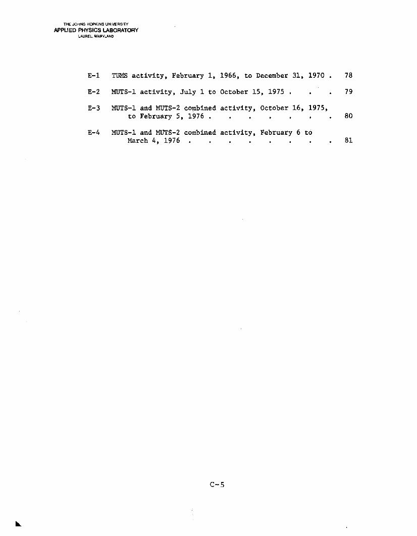
E-1 TUMS activity, February 1, 1966, to December 31, 1970 • 78
E-2 MUTS-1 activity, July 1 to October 15, 1975 • 79
E-3 MUTS-1 and MUTS-2 combined activity, October 16, 1975,to February 5, 1976 • 80
E-4 MUTS-1 and MUTS-2 combined activity, February 6 toMarch 4, 1976 81
C-5

THE JOHNS HOPKINS UNIVERSITY
APPLIED PHYSICS LABORATORYLAUREL, MARYLAND
TABLES
1
2
3
4
TUMS microwave power density model
First MUTS survey
Second MUTS survey •
MUTS microwave power density model
C-6
33
42
45
48
THE JOHNS HOPKINS UNIVERSITY
APPLIED PHYSICS LABORATORYLAUREL, MARYLAND
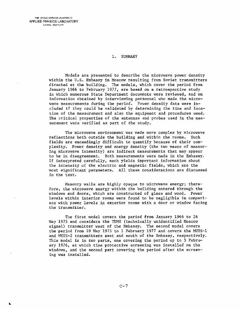
1. SUMMARY
Models are presented to describe the microwave power densitywithin the U.S. Embassy in Moscow resulting from Soviet transmittersdirected at the building. The models t which cover the period fromJanuary 1966 to February 1977, are based on a retrospective studyin which numerous State Department documents were reviewed, and oninformation obtained by interviewing personnel who made the microwave measurements during the period. Power density data were included if they could be validated by determining the time and location of the measurement and also the equipment and procedures used.The critical properties of the antennas and probes used in the measurement were verified as part of the study.
The microwave environment was made more complex by microwavereflections both outside the building and within the rooms. Suchfields are exceedingly difficult to quantify because of their complexity. Power density and energy density (the two means of measuring microwave intensity) are indirect measurements that may appearto be in disagreement. Both measurements were made in the Embassy.If interpreted carefullYt each yields important information aboutthe intensity of the electric and magnetic fields t which are themost significant parameters. All these considerations are discussedin the text.
Masonry walls are highly opaque to microwave energy; therefore, the microwave energy within the building entered through thewindows and doors t which are constructed of glass and wood. Powerlevels within interior rooms were found to be negligible in comparison with power levels in exterior rooms with a door or window facingthe transmitter.
The first model covers the period from January 1966 to 26May 1975 and considers the TUMS (technically unidentified Moscowsignal) transmitter west of the Embassy. The second model coversthe period from 28 May 1975 to 1 February 1977 and covers the MUTS-land MUTS-2 transmitters east and south of the EmbassYt respectively.This model is in two parts t one covering the period up to 5 February 1976, at which time protective screening was installed on thewindows, and the second part covering the period after the screening was installed.
C-7

THE JOHNS HOPKINS UNIVERSITY
APPLIED PHYSICS LABORATORYLAUREL, MARYLAND
For TUMS, power density was measured directly. Inside therooms having the highest levels, the power density within antinoderegions (areas in which reflections reinforced the direct signal)
was about 4 ~W/cm2 within 2 ft of the door or window, and 2.5 ~W/cm2elsewhere in the room.* The average power density in these rooms
was about 1.5 ~W/cm2. In interior rooms and in exterior rooms not2on the west wall, power density was less than 0.1 ~W/cm •
During the MUTS interval, electric-field energy density wasmeasured and the "equivalent" power density calculated.** The firstportion of the MUTS model extends from 28 May 1975, when MUTS-l appeared, to 5 February 1976, when the installation of window screening and also reductions in transmitter power reduced power levels
inside the building to very low levels (approximately 0.002 ~W/cm2).Prior to the screening, at locations near upper-story windows onthe east and south walls of the central building, the power density
2within antinodes averaged 3.3 ~W/cm ; within these rooms the average2antinode measured 2.2 ~W/cm. The average value throughout these
exterior rooms would have been lower, and 1.5 ~W/cm2 could be considered as a representative number. The power density was lower inthe living quarters of the central building and on all floors ofthe north and south wings.
The MUTS beam was more intense toward the upper southeastcorner of the central building. While the values above were thoseaveraged for all rooms on the upper floors of the central building,
2several rooms had antinode intensities of 7 to 10 ~W/cm. Typicallevels within those rooms would be about half of the antinode level
(i.e., 3.5 to 5 ~W/cm2).
These values are long-term averages; the signal level didvary, although generally not to any great extent. In areas of thebuilding in which personnel were exposed, the highest power density
2recorded throughout the entire study was 24 ~W/cm in Room 1001 on24 January 1976. This occurred during a two hour period of unusualsignal strength. Excluding values recorded during this brief in-
2terval, the next highest level was 10.2 ~W/cm near the window inRoom 1003 in late July 1975. Both measurements were at electricfield antinodes.
*See Appendix D for a discussion of the measurement units used inthe text.
**See Section 2 for a discussion of power density and energy density.
C-8

THE JOHNS HOPKINS UNIVERSITY
APPLIED PHYSICS LABORATORYLAUREL, MARYLAND
The second portion of the MUTS model extends from 5 February1976, when protective screening was installed, to 1 February 1977,the end date of the study. During this period, the MUTS power den
2sity within all rooms of the Embassy was 0.1 ~W/cm or less. The2intensity on the rooftop was about 2 ~W/cm •
After introductory sections that discuss the problems involved in evaluating microwave intensity measurements made withina reflective environment, the text describes the sequence of eventspertaining to each signal, its spectrum, the region of exposure,the critical measurements used in defining the fields, and finallythe power density model itself. The few equations included aresupplementary. They are not essential to the discussion.
Records of transmitter operating hours were maintained atthe Embassy. Summary charts showing the percentage of time thesignal was recorded are presented in Appendix E. The record is notcontinuous because time charts could not be found for some intervals.
It must be emphasized that this study was as much a historical as a technical exercise; therefore, it is subject to all theinherent limitations of any attempt to reconstruct the past. Withthe exception of a few interviews, all the evidence available wasthat contained in a collection of State Department documents. Inany such collection, assembled over a period of years, there willbe conflicting statements, outright errors, typographical mistakes,and missing documents. Such problems could usually be resolved byother documents written within the same time frame. Less frequently,the general context of a group of documents had to be considered.On rare occasions, the writer had to make a judgement based on hisown knowledge of antennas and measurement problems. The writer believes that the power density models proposed in this report are asaccurate and as detailed as the body of evidence will allow.
C-9

THE JOHNS HOPKINS UNIVERSITY
APPLIED PHYSICS LABORATORYLAUREL, MARYLAND
2. POWER DENSITY AND ENERGY DENSITY
Measurements prior to 1975 were made using a beam-formingmicrowave antenna such as a horn. Subsequent data were recordedusing the probe of an electric-field energy density meter. In both
cases, the results are stated in power density units (~W/cm2) inorder to allow a comparison to various radiation standards. Thebeam antenna may be used to determine power density by measuringreceived power and then dividing by the calibrated effective areaof the antenna (see Appendix A). The energy density meter, as itsname implies, measures total electric-field energy density (seeAppendix B). Energy density readings have been converted into"equivalent" plane-wave power densities by multiplying by 2 timesthe speed of light. Such a conversion is valid only under planewave conditions. Within more complex fields, the conversion of energy density to power density will yield excessively high valuesif the reading is taken in a local electric-field maximum. Becausethe evidence shows that all data in the Embassy were recorded in acomplex RF (radio frequency) environment with many microwave reflections, it is essential that the difference between power densityand energy density be understood, as well as the limitations of theequivalent plane-wave power density concept. This in turn requiressome familiarity with the concepts of a propagating plane wave andof a standing wave.
At distances not in the immediate vicinity of the source, asimple RF electromagnetic wave consists of uniform electric and magnetic force fields oriented at right angles to each other and transverse to the wave's direction of propagation. This simple wave iscalled a "plane wave" because at large distances from the source thewavefront is relatively flat. The electric and magnetic forces alternate in intensity and direction at the signal frequency; at anylocation and instant they are in phase. The changing magnetic fieldgenerates an electric field, and vice versa. This is the process,described by Maxwell's equations, through which electromagneticwaves radiate and carry energy away from their source. Each fieldcomponent contains half the energy of the wave. At a given location, the local field is completely described if the magnitude,the orientation, and the direction of propagation of either component is known. From that information, the other field component,
the power density (in W/cm2), the total energy density (in J/cm3),and the energy density of either component may be calculated. Ifthe field orientation (polarization) and anyone of the densityquantities are known, all the other quantities may be calculated.
C-IO

THE JOHNS HOPKINS UNIVERSITY
APPLIED PHYSICS LABORATORYLAUREL, MARYLAND
In a simple plane wave, all these quantities are related to eachother unambiguously, and anyone quantity plus polarization isenough to evaluate any potential hazard.
As an example, the electric-field energy density at any pointis proportional to the square of the electric field strength. Asimilar relationship defines the magnetic-field energy density.Total energy density is the sum of the two. Power density is therate at which energy crosses a transverse unit area averaged overa time interval equal to one RF cycle. For the plane wave, theelectric and magnetic energy densities (u and u ), power density
e m(PD), and peak (as opposed to rms) field strength vectors* are related to each other as follows (Refs. 1 and 2):
PD 1 IRe(E x H*)I = !~IEI2 = !~IHI2= -2 2 II 2 e:
1 (E • E*) 1 lil 2,u = - e: = - e:e 4 4
and
1 (H • H*) 1IHI
2•u =-ll =7;1lm 4
The vertical bars denote the vector's total magnitude, and the asterisk indicates use of the complex conjugate.** The total energydensity (ut ) is
u = u + ut e m
*These fields alternate with time in the form of a sine wave. The"effective" or rms (root-mean-square) value of a sinusoid is l/'Vrof the peak value. This is the hypothetical static (DC) valuethat would produce the same average power as the alternating (AC)field. A vector has both magnitude and direction. The force ofgravity is a vector force.
**Complex numbers are two-dimensional, they are frequently used inphysics and engineering.
C-ll
THE JOHNS HOPKINS UNIVERSITY
APPLIED PHYSICS LABORATORYLAUREL, MARYLAND
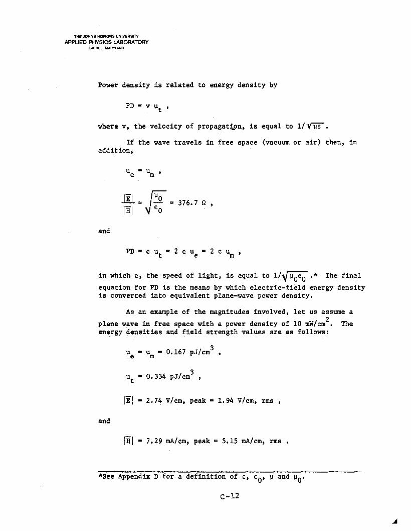
Power density is related to ener~y density by
PD ... v ut '
where v, the velocity of propagatton, is equal to 1/~.
If the wave travels in free space (vacuum or air) then, inaddition,
u .. ue m
and
Iii ftfo~... - III 376.7IHI e:o
n ,
PD ... c u ... 2 c u ... 2 c ut e m
in which c, the speed of light, is equal to l/"~OeO.* The final
equation for PD is the means by which electric-field energy densityis converted into equivalent plane-wave power density.
As an example of the magnitudes involved, let us assume a
plane wave in free space with a power density of 10 mW/cm2• Theenergy densities and field strength values are as follows:
u .. u .. 0.167 pJ/cm3 ,e m
ut .. 0.334 pJ/cm3 ,
Iii" 2.74 V/cm, peak III 1.94 V/cm, rms ,
and
IHI • 7.29 mA/cm, peak ... 5.15 mA/cm, rms •
*See Appendix D for a definition of e:, e:O' ~ and ~O.
C-12

THE JOHNS HOPKINS UNIVERSITY
APPLIED PHYSICS LABORATORYLAUREL, MARYLAND
This power density is the maximum allowed by the U.S. electromagnetic radiation criterion (Ref. 3). The corresponding rmsfield strengths approximate the limiting field strengths in thereference.
Once again, these relationships are valid at any location
in a plane wave. In free space, a single quantity (Iii, IHI, u ,e
um' ut ' or PD) is sufficient to determine all the others. There-
fore, any of the parameters could serve as an indicator of potential biological hazard.
are present in addition to the direct
IHI will vary with location, as will thatis no way to calculate power density from
If reflected waves
wave, the ratio of Iii toof u to u. Also, theree man electric-field or magnetic-field energy density measurement, orvice versa. As an extreme example, consider a large electricallyconducting sheet placed broadside to the direction of propagation
of the 10 mw/cm2 plane wave described above. At each point in frontof the sheet, the electric and magnetic field is'the sum of the direct and reflected components. However, the electric field undergoes an instantaneous reversal of orientation when it is reflected,whereas the magnetic field does not. A stationary oscillatory fieldstructure appears before the sheet. As in hydraulics or acoustics,this fixed pattern is called a "standing wave." Because of theasymmetry at reflection, the antinodes and nodes (stationary regionsof maximum and minimum oscillations) are located at different pointsfor the electric and magnetic fields. Adjacent to the sheet and athalf-wavelength intervals before it, the magnetic field is twice itsoriginal strength and the electric field is zero. The standing wavepattern for the electric field also repeats at half-wavelength intervals, but it is shifted by one-quarter wavelength so that thereis a minimum at the reflector. The total electric field intensityis doubled at each antinode, and the magnetic field is zero at theselocations.
The implications of this complexity are as follows. If anelectric field or magnetic field energy density meter were used toprobe the field before the sheet, the energy density would no longerbe uniform but would rise and fall (alternately for the two meters)as the probe was moved away from the sheet. At an electric-fieldantinode, the field is doubled and the electric-field energy den-
sity is 0.667 pJ/cm3, four times that of the original plane wave.There is no magnetic field at this location, but if the plane-wave
C-13
THE JOHNS HOPKINS UNIVERSITY
APPLIED PHYSICS LABORATORYLAUREL, MARYLAND
formula were followed to convert to equivalent plane-wave powerdensity (multiplying by 2 to account for the magnetic energy in aplane wave and then multiplying by the speed of light) the electricfield energy density converts to an equivalent power density of
240 mW/cm , four times that of the incident plane wave.
If, instead of an electric-field energy density meter, ahorn antenna and power meter were used to measure power density
directly, a reading of 10 mW/cm2 would be obtained with the hornpointing toward the source, and an identical reading would resultwith the horn turned to point at the reflecting sheet. The hornresolves the incident and reflected waves and reads the power density of each.
When used in the standing wave, an energy density meter would
indicate an equivalent power density of 40 mW/cm2 , while the horn
resolves two separate waves, each with a 10 mW/cm2 power density.If taken at face value, these two methods of measurement, each validin a plane wave, would lead to different evaluations of the field.
There are two errors implicit in this comparison. Both aredue to the phenomenon of interference (constructive and destructive)between the incident and the reflected wave. First, the conversionof electric-field energy density to equivalent power density may bein error by an amount depending on the relative magnitude of the reflected wave. The second error is that the electric and magneticfield strengths of the two waves are additive (as vectors) at eachpoint in space, but their power densities are not. The actual power density in a standing wave is zero. There is no time-averagedenergy flow at any point. Energy oscillates back and forth betweenthe electric and magnetic antinodes at twice the RF frequency.
In the presence of microwave reflections, the power densitycriterion is an inconsistant measure of biological hazard. Despitethe conflicting readings above and the fact that the standing wavehas no power density, the internal fields induced within a man-sizedobject at microwave frequencies would not be greatly different than
those caused by the initial 10 mW/cm2 plane wave. If far enoughfrom the reflecting sheet to avoid any shadowing effects, the frontof the relatively large object would be exposed only to the incidentwave and the rear only to the equally intense reflected wave.
The next section will show that the ambient electric and
magnetic fields (E and H) are the cause of any biological effects.These fields are extremely difficult to measure adequately, and
C-14

THE JOHNS HOPKINS UNIVERSITY
APPLIED PHYSICS LABORATORYLAUREL, MARYLAND
power density or energy density serve only as simplified and moremeasurable substitutes. In the example above, in which an electricfield energy density meter and a horn were used one at a time tomeasure the standing wave, either measurement (plus the variationas the probe or antenna were moved) would allow the observer toevaluate the total magnitudes of the electric and magnetic fields
(Iii and IHI) in the area.
As an indication of the extent to which a single relativelyweak reflection can distort the total field, consider an obliquereflection in which the reflected electric-field is 12 dB* less thanthat in the incident field (Er/Ei = 0.25). The standing wave ratio
is defined as the ratio of the maximum to minimum in the total fieldresulting from the interference of the direct and reflected waves.In this case,
SWR
This corresponds to power density or energy density variations equalto the square of the SWR. In this case, the reflection would causethe power density to vary by a ratio of 2.8:1, or 4.5 dB.
Although in radiation hazard surveys it is common to measuremaximum electric-field energy density and convert to equivalent
*The dB (decibel) is a compressed logarithmic unit used to expressa power ratio that may vary over many orders of magnitude:
The unit may be used as defined in this case for power density orenergy density ratios. Since both are proportional to the squareof either electric or magnetic field strength, the unit can be restated in those terms as
A 6 dB change corresponds to a factor of 4 change in power, or afactor of 2 change in field strength (these changes are equivalent,in terms of power).
C-15

THE JOHNS HOPKINS UNIVERSITY
APPLIED PHYSICS LABORATORYLAUREL, MARYLAND
plane-wave power density (this was done in Moscow during the 1975and 1976 interval), the above example shows that this conversionis ambiguous in an environment with standing waves.
Within the Embassy, the environment included reflectionsfrom outside the building, from the window frames of the Embassy,and from walls and objects inside the rooms. Standing wave nodesand antinodes would appear in combination with spatial variationsin power density (caused by the combination of the direct and reflected components). The measured field would show great complexity,whether measured with an isotropic energy density meter (sensitiveto reflections from all directions) or with a horn antenna of relatively narrow beamwidth (capable of receiving only the direct andforward-reflected waves and reading power density directly).
To summarize this section, several points may be restated.Because of the complex wave pattern within the rooms of the Embassy,a power density field probe using a microwave horn will differ fromthat using an electric-field energy density meter. While both measurements are subject to significant error, either may be used witha degree of caution to evaluate the magnitude of the ambient electric and magnetic fields.
If a horn antenna is used, power density is determined bydividing received power by the antenna's effective area. Uncertainties are introduced by the complex spectrum of the signal (see Appendix A) and by various forward reflections. If the antenna'saperture size is increased (thus decreasing beamwidth) in an effortto reject the reflected waves, then spatial resolution is degraded.The corresponding magnitudes for the resultant electric and magnetic
fields (Iii and IHI) for all sources within the beam are approximately determined by the plane wave relationships. These fieldstrength values are plotted versus power density in Fig. 1. The Eand H fields may be considered coincident and in phase at the location of the measurement. The measurement would not show the effectof reflections coming from outside the antenna's beamwidth.
The electric-field energy density probe was only a smallfraction of a wavelength in size; it can resolve small-scale variations in the total electric field. It measures the resultant ofwaves radiating from all directions. While it yields an accuratereading of electric-field energy density, and hence the magnitudeof the electric field, a conversion into equivalent plane-wave power density is accurate only if the field consists of a single planewave. If, in more complex fields, the energy density reading istaken at an antinode (as was done in all measurements within the
C-16

,.
~ "....
C:I
:m
m Ca~"i
c:::
I:cn
"-<
:I:
J!!~~
;:°2
5~cn~
~>c:
Zm~
"oiii
:OiJl
~~
o ~
2en E ....
1E
'0.
8-
0.6
« -0.
4I -0
'
0.2
~ CJ
.+"
0.1
~0.
08g>
0.06
~
0.04
(mW
/cm
2)
46
81
010
02
1
1000
100
46
810
0.02
II
Jr
II
II
II
II
II
II
II
II
II
II
II
II
II
I10
.01
1000
800
600
400
_2
00
CI) E ....,
100
E80
:>6
0- w
40
()
~20
I~
..... -..J
CJ ';:
10t)
8~
6 4 2 1 12
(J,L
W/c
m2
)
Plan
e-w
ave
pow
erde
nsit
y
Fig
.tP
lane
.wav
eel
ectr
ican
dm
agne
tic
fiel
dst
reng
th(f
ree
spac
e).

THE JOHNS HOPKINS UNIVERSITY
APPLIED PHYSICS LABORATORYLAUREL, MARYLAND
Embassy, because the highest levels were being sought), the equivalent power density is always greater than the actual power densityat that point due to the implied level of the magnetic field (whichis greater than that likely to exist at the electric antinode).This bias, unless interpreted with care, may lead to an overestimation of any potential RF hazard. Also, RF magnetic fields are notdetected by an electric-field energy density meter. It may be assumed that if a complex field has electrical antinodes of a certainenergy density then equally intense magnetic antinodes exist, although probably not at the same locations.
Figure 2 shows the conversion from the electric-field (ormagnetic-field) energy density measurements to the equivalent planewave power density. Figure 1 may then be used to find the fieldscorresponding to this value of power density. If reflections weresignificant, as they were for all the Embassy measurements, theseE and H field strengths should not be regarded as existing in phaseat the same location. The field values may correspond to those inseparate electric and magnetic antinodes.
C-18

THE JOHNS HOPKINS UNIVERSITY
APPLIED PHYSICS LABORATORYLAUREL, MARYLAND
4 6 10-124 6 10-16 2 4 6 10-15 2 4 6 10-14 2 4 6 10-13 2
Energy density (J/cm3 )
Fig. 2 Energy density to equivalent plane-wave power density conversion.
64
2
10-6 '--..L.L_--I.---I.-L-l-_...I..----I---l---l-..l.----l_---l-.---l-.....L...J._---l-._...I..-..1-J'-I-_..L.-----I.---l--L..J
10-17 2
2
10-5
64
10-1r'----r-~-r-r-r--,--,----,r__r__.____,-__r__r.,...,-_,_-.,._.,._...._r_-_r___,__,__,_,
64
10-2 ....-.10 mW/cm2 (U.S. radiation criterion)
64
2
2
La>~ 10-4oa..
('II
510-3
~ 6~ 4'c;;c~ 2
C-19

THE JOHNS HOPKINS UNIVERSITY
APPLIED PHYSICS LABORATORYLAUREL, MARYLAND
3. THE ABSORPTION OF MICROWAVES BY MATTER
Section 2 has shown that the electric and magnetic fieldstrengths corresponding to either directly measured power densityor equivalent power density may be determined from Fig. 1. Thecritical difference is the spatial and temporal differences in thedistribution of the fields. In the direct case, in which power density is measured by a horn, the electric and magnetic fields existat the same point and are maximum at the same time. This, on alocal scale, is the condition corresponding to a maximum transferof energy. For the equivalent power density, the E and H fieldsreach their maximums at different times and at displaced locations.
Power density values alone are not sufficient to describethe microwave fields within the Embassy. For TUMS, power densitywas measured directly; for MUTS equivalent power density valuesare presented. The electric and magnetic fields in either casewere equally distorted by microwave reflections, and their spatialand temporal characteristics were generally the same (i.e., exceedingly complex) within the Embassy rooms. It should be noted thateven at the same point in such an environment, the power density asmeasured by the two methods will differ and so will the E and Hfield strengths inferred from the measurements. The equivalentpower density will be the higher if read at an electric-field antinode, but the inferred higher E and H fields are not simultaneousand colocated. The direct power density is lower, but its lower Eand H fields are oriented to allow a more efficient transfer ofpower. The differences are subtle, and they may not even be important, but they must be known by those who judge the effect of thesecomplex fields, because they will affect the way in which energy iscoupled into an object exposed to such a field.
In order to understand the differences, some understandingis required of the mechanism by which biological tissue absorbsmicrowave energy. This will be done on a microscopic scale andfrom an engineer's viewpoint. The discussion will show that whileall significant absorption must be caused by the internal electricfield, this field depends on both the external incident electric andmagnetic fields. These vector fields are difficult to measure ina complex reflective environment. Twelve values are required todefine both the electric and magnetic fields at a single point inspace. Power density and energy density are useful because theyare more readily measured and because either can be used to estimate the actual magnitude of the individual fields.
C-20

THE JOHNS HOPKINS UNIVERSITY
APPLIED PHYSICS LABORATORYLAUREL, MARYLAND
According to classical electromagnetic theory, the followingis the sequence of events by which a radio frequency electromagneticwave loses energy and interacts with matter. When an object is exposed to an RF electromagnetic field, alternating electric and magnetic force fields are induced on its surface. The induced surfacefields depend not only on the incident external fields but also onthe size, shape, material composition, and orientation of the object. These alternating fields (specifically, the components tangent to the surface of the object) act as the generating source fortwo additional and very complex electromagnetic waves. One is thescattered wave, which reflects energy away from the object, and theother is the transmitted wave, which penetrates into the object.The penetrating wave is the one of interest.
Theoretically, if the composition of the object is known interms of electromagnetic constants describing its various constituent parts, a definition of either the tangential electric or thetangential magnetic field over the surface of the body (the totalfield at each point due to the incident, scattered, and penetratingwaves) is sufficient to allow a complete description of the verycomplex fields anywhere within its interior (Ref. 4). The entiresurface must be considered. Turning this statement around, itsmeaning is that either the electric or the magnetic field on thesurface may be considered the cause of all subsequent internalevents. It also means that the spatial and temporal variations ofthis field are of importance.
At RF frequencies, the incident electric and magnetic fieldsare equally important in the evaluation of a possible radiationhazard. In a complex field environment, the degree of hazard de-
pends directly on the two vector field strength parameters (E and
H) and only indirectly on more measurable combinations of theseparameters (such as power density or energy density).
Although the electric and magnetic fields are of equal importance outside the object, on the inside it is the internal electric field through which energy is dissipated. The internal magnetic and electric dissipation mechanisms are discussed separately.
There are two ways in which an internal magnetic field maydissipate energy. The first is through the direct action of thealternating magnetic field on magnetic materials. This requires
C-21

THE JOHNS HOPKINS UNIVERSITY
APPLIED PHYSICS LABORATORYLAUREL, MARYLAND
the presence of a ferromagnetic material in which the alternatingfield loses energy through hysteresis. This property is extremelyrare in biological tissue (Ref. 5) and is of no interest here.*
The second magnetic interaction is through a force exertedon a moving charged particle such as an ion. If a charged particleis exposed to electric and magnetic fields, the resultant forcevector is
F=q(E"+ (v x 'B)] ,
in which v is velocity, B = ~OH, and q is the charge.** Individu
ally the two forces are
F = qEe
and
F = q(v x "B)m
The ratio of the electric force to the maximum magnetic force is
*Some bacteria, molluscs, and arthropods are able to synthesizemagnetite (Fe
30
4). This mineral has also been found in the heads
and necks of pigeons. Bacteria and pigeons are known to be ableto orient themselves according to weak magnetic fields. In thecase of pigeons, flight experiments on cloudy days have shown thebirds capable of sensing magnetic field alterations on the orderof 1/500 of the earth's field strength.
**The operator "x" denotes vector multiplication. The resultant
force vector F is perpendicular to both v and B. Its magnitudem
is [q Ivl IBI sin e], in which e is the angle between the direc-
tions of v and B.
C-22
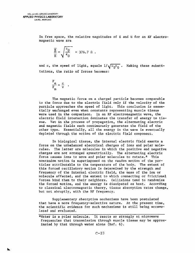
THE JOHNS HOPKINS UNIVERSITY
APPLIED PHYSICS LABORATORYLAUREL, MARYLAND
In free space, the relative magnitudes of E and H for an RF electromagnetic wave are
376.7 Q •
and c, the speed of light, equals l/"~OEO' Making these substi
tutions, the ratio of forces becomes:
Fe c-=
F vm
The magnetic force on a charged particle becomes comparableto the force due to the electric field only if the velocity of theparticle approaches the speed of light. This conclusion is essentially unchanged even when constants representing muscle tissuewere used in the comparison. In an RF electromagnetic wave, theelectric field interaction dominates the transfer of energy to tissue. Yet in the process of propagation, the alternating electricand magnetic fields each continuously generates the field of theother type. Essentially, all the energy in the wave is eventuallydepleted through the action of the electric field component.
In biological tissue, the internal electric field exerts aforce on the unbalanced electrical charges of ions and polar molecules. The latter are molecules in which the positive and negativecharges are not arranged symmetrically. The alternating electricforce causes ions to move and polar molecules to rotate.* Thisnonrandom motion is superimposed on the random motion of the particles attributable to the temperature of the body. The extent ofthis forced oscillatory motion is determined by the strength andfrequency of the internal electric field, the mass of the ion ormolecule affected, and the extent to which connecting or frictionalforces bind them to their neighbors. Collisions tend to randomizethe forced motion, and the energy is dissipated as heat. Accordingto classical electromagnetic theory, tissue absorption rates change,but not abruptly, with the RF frequency.
Supplementary absorption mechanisms have been postulatedthat have a more frequency-selective nature. At the present time,the scientific evidence for such mechanisms is still being accumulated and evaluated.
*Water is a polar molecule. It reacts so strongly at microwavefrequencies that transmission through muscle tissue may be approximated by that through water alone (Ref. 6).
C-23

THE JOHNS HOPKINS UNIVERSITY
APPLIED PHYSICS LABORATORYLAUREL. MARYLAND
In summary, it is through the action of the internal electricfield that all but a small fraction of the energy contained in theinternal electromagnetic wave is converted into kinetic energy ona microscopic scale within the tissue. The internal electric fieldin turn is generated by the incident electric and magnetic fieldsover the surface of the body. These two external components areequally important. Their spatial and temporal variations must beconsidered. Power density and energy density are of value becausethey are more easily measured and because they serve as approximateindicators (in a reflective environment) of the incident electricand magnetic fields.
C-24

THE JOHNS HOPKINS UNIVERSITY
APPLIED PHYSICS LABORATORYLAUREL, MARYLAND
4. TUMS
TUMS SEQUENCE OF EVENTS
TUMS was a horizontally polarized signal consisting of anumber of discrete frequency components distributed between 2.58and 4.10 GHz. It was transmitted from a fifth floor window of anapartment building 100 yards west of the Embassy. The signal mayhave been in existence from time to time as early as 1953, but itwas not until the early 1960's that the necessary equipment was onsite to characterize its parameters adequately (Ref. 7). At thattime, an activity monitor was installed on the tenth floor to record intervals of TUMS transmission on a continuous strip-chart.(Figures that describe and summarize the percent operating time forthe TUMS transmitter are presented in Appendix E.) This record wasmaintained over the years and supplemented from time to time bypower density measurements taken at various window locations onthe west side of the central Embassy building. The intensity ofthe TUMS signal appears to have been relatively constant over theyears. It was turned off permanently on 26 May 1975. Two dayslater the MUTS-1 transmitter initiated daily operation from itsrooftop location facing the east side of the Embassy.
TUMS REGION OF EXPOSURE
While TUMS initially was thought to be directed against thesouthern half of the west wall of the central building, the actualextent of the beam is not precisely known. The beam shape had tobe inferred from various series of measurements at available windowlocations. The mu1tipath environment at those windows, compoundedby the differing frequency content of the three operating modes,has tended to obscure the shape of the beam. In 1963 the beam wasdescribed as 50 feet in width across the building (Ref. 8). Subsequent documents imply a wider beamwidth (Refs. 9 and 10). Aseries of measurements in 1967 (Refs. 11 and 12) show that the entire height of the building was irradiated. While no measurementsappear to have been taken near the north end of the building, fromthe broad vertical beamwidth it appears likely that the entire westwall of the central building was illuminated. At various times,maximum intensity was recorded at different locations between thethird and ninth floors (Ref. 13). This variation is probably causedby mu1tipath propagation and the changing frequency content of thetransmission rather than to any directional properties of the transmitter. For the purpose of establishing the model, maximum and
C-25

THE JOHNS HOPKINS UNIVERSITY
APPLIED PHYSICS LABORATORYLAUREL, MARYLAND
uniform intensity is assumed from the third to the ninth floor ofthe west side of the main building, with lower levels on the otherfloors and at the apartments over the north and south entrances tothe courtyard.
In essence, all energy entering the Embassy did so throughglass (or in one case, wooden) windows on the illuminated wall andwas dissipated within the adjacent room. Exposure was limited tounshielded rooms* having a window on the illuminated wall. Thecalculated average transmission loss of double-glazed windows was0.66 dB, although for some frequencies the loss was as high as2.4 dB. (This calculation was made over a frequency range containing several complete reflection cycles to reduce errors due to dimensional uncertainties. It is described in Appendix C.) A measu~ement at APL showed that the transmission loss of masonry wallsis ~30 dB and that levels in interior rooms were 10 dB (a factor of10 in power) or more lower than in exterior rooms with windows (Ref.14). During the July 1975 MUTS survey at the Embassy (Ref. 15),power levels in the rooms not directly exposed were below the sensitivity of the instrument. Furthermore, at these frequencies, noenergy would be transmitted to other regions of the building bytelephone or power lines, water pipes, etc.
TUMS SPECTRUM
TUMS typically consisted of seven independent relatively narrowband components within the total band between 2.58 and 4.10 GHz.The components could differ in level by as much as 10 dB. The bandwidth of each was usually between 0.5 and 15 MHz. Narrowband components typically showed discrete subcomponents indicating 440 Hzmodulation (usually AM). Wideband components had both 440 Hz andnoise modulation.
The components were distributed across the band differentlyin each of the three operating modes. These modes are named according to the relative spectral concentration of the components. Thefollowing shows a sample distribution:
High mode - 3.08 to 3.39 GHz (7 components)
Medium mode - 2.65, 2.74, 4.01, 4.02, 4.05, 4.06, 4.08,and 4.10 GHz
Low mode - 2.61, 2.75, 2.84, 3.55, 3.58, 3.62, and3.67 GHz
*For security purposes, some Embassy rooms were shielded with metalto prevent penetration by or leakage of electromagnetic fields.
C-26

THE JOHNS HOPKINS UNIVERSITY
APPLIED PHYSICS LABORATORYLAUREL, MARYLAND
When changing from mode to mode, components would be retuned orturned on or off. Each mode usually persisted for several hours.During mode changing, a high power condition could occur lastingfrom 10 seconds to 2 minutes. In 1967, the level of this transient
was described (Ref. 16) as "of the order of 20 llW/cm2 within theapartments or offices on the west face of the building" and in 1971
as rising to the 10 llW/cm2 level (Ref. 17).
TUMS emissions occasionally contained a much lower level ofenergy between 8 and 10 GHz. In 1972 this was once observed in theabsence of lower frequency radiation (Ref. 18).
TUMS CRITICAL MEASUREMENTS
This section reviews, in sequence, the power measurementsfrom which usable data could be extracted to establish a power density model. While many power density numbers were found in thedocuments, a large portion were unusable for a retrospective studybecause they contained no description of how or where the measurements were made. Many documents were found with partial documentation of the measurement conditions. Only by comparing fragmentaryinformation from a number of documents could sufficient informationbe collected to allow an evaluation of a stated power density number. The required information included:
1. The location of the measurement both within the buildingand with respect to the window of the room,
2. Calibration data on the antenna used and some description of the characteristics of the detector,
3. How the measurement was made (i.e., the substitutionmethod for each component or an integrated reading bymeans of a heat-sensitive thermistor and power meter),and
4. Whether the antenna was fixed at an arbitrary locationor was moved about to find the local region of highestsignal level.
Aperture antennas such as microwave horns were used to directly measure TUMS power density. This procedure differed fromthat used later for MUTS, in which the electric-field energy density was measured and the equivalent power density calculated.Aperture antennas are polarized and directional and receive only
C-27

THE JOHNS HOPKINS UNIVERSITY
APPLIED PHYSICS LABORATORYLAUREL, MARYLAND
the matched polarization component from within their beam angles.TUMS was horizontally polarized, and the antennas were positionedto receive this component. Their half-power beamwidths vary from18 to 65°, depending on the frequency and the particular antenna.In all cases, the antenna beam was directed toward the source. Inthis orientation, power density equals power received divided bythe effective area (not the physical area) of the antenna. Effective area, Aeff , is derived from the antenna's power gain ratio as
G>..2A =eff 47T
where >.. is the wavelength.from a calibration chart.than one with a wide beam.in detail in Appendix A.
Gain may be determined for each antennaA narrow-beam antenna has a higher gain
Gain and effective area are described
Effective area is a function of frequency and can vary by asmuch as 2.5 to 1 across the TUMS band. This introduces an uncertainty in the computation of the power density for a complex wideband signaL For the present study, gain data were obtained on allantennas involved and their effective areas calculated. Usually,specific information on the frequency content of the TUMS signalat the time of measurement is not available. In those cases, theaverage antenna effective area over the TUMS band (2.58 to 4.10 GHz)was used to calculate power densities for this report. In somecases, this value differs somewhat from that reported at the timeof measurement.
A description of the antennas used, including gain and effective area data, is included in Appendix A.
No measurements were found prior to 1966 that included agood enough description to be included in this study. One 1965document (Ref. 19) asks for a clarification of a heresay value of
22 dBm/m2 (16 llW/cm2) "on the surface of the building" (the power
density unit dBm/m2 is defined in Appendix D). Although no answering document was found, verification must not have been forthcoming,since the same writer (who made many of the measurements during thelate 1960's) states repeatedly in later documents his belief thatthe Soviets intentionally kept the level below their industrial
standard of 10 llW/cm2 • Reference 9 contains the statement that"total power level per square meter at the windows of the Embassy
was computed in November 1965 as +13 to +17 dBm/m2
" (2 to 5 llW/cm2).
C-28

THE JOHNS HOPKINS UNIVERSITY
APPLIED PHYSICS LABORATORYLAUREL, MARYLAND
Other documents indicate that maximum intensity at this time wason the ninth floor at the second window from the south end.
In April 1966, a power density measurement was made in theTUMS observation room.* That room differed from all other roomsin the Embassy in that the inner pane of the double-glazed windowwas removed and replaced with a sheet of one-quarter inch plywood.In order to relate measurements made within this room to those madeelsewhere, transmission loss calculations for this window configuration and for the normal windows were made for this study (seeAppendix C). The TUMS observation window has an average transmission loss over the TUMS band of 0.5 dB, although at some frequenciesits loss can be as high as 1.5 dB. The ordinary double-glazed windows have an average loss of 0.7 dB, with a maximum loss of 2.4 dB.For the purpose of the study, both window configurations are considered to be low-loss and similar in transmission characteristics.Therefore, measurements made within that room may be consideredrepresentative of the levels within nearby rooms.
A Po1arad CA-S horn was mounted behind the plywood windowand connected to a Po1arad receiver. One frequency component wastuned at a time and its power measured by substitution with anequal signal from a calibrated signal generator (Ref. 20). Themeasurement continued while frequency components were added or deleted until a total of 13 components had been measured. Power density was calculated for each component by dividing by the effectivearea of the horn. (This calculation was done erroneously in Ref.20. Someone had later penciled in corrections, and the writer hasmade an additional small correction to use more accurate values forthe effective area.) The power density of the 13 components mea-
sured varied over a 65:1 range. Their average is 0.44 ~W/cm2, andthis is significantly weighted by the two strongest components at3.320 and 3.347 GHz. Using this average value, and the fact thatTUMS usually contained only seven simultaneous components, the typical power density at the arbitrary location behind the TUMS obser-
vation window is 3.1 ~W/cm2.
*Monitoring equipment was installed in that room (on the ninthfloor just north of the central stairway) to allow the TUMS spectrum to be observed. The location was separate from that of theTUMS activity monitor, which provided only a simple record of thesignal's operating hours.
C-29

THE JOHNS HOPKINS UNIVERSITY
APPLIED PHYSICS LABORATORYLAUREL, MARYLAND
Several documents refer to a power reduction occurring inMarch or April 1967. This is the only time during the entire periodof TUMS transmissions that a long-term power change was believed tohave occurred, yet the evidence that a decrease occurred is not convincing. Reference 21 describes a decrease in power level in April1967 as indicated by the TUMS strip-chart activity monitor. As confirmation, a measurement of the signal in the window area location
2 2that had yielded a +17 dBm/m (5 ~W/cm ) level in November 1965 now
implied a level of +11 dBm/m2 (1.3 ~w/cm2). In contrast, a 1972document (Ref. 22) refers to a power decrease of only 25% since TUMSwas initially measured. The difficulty with these measurements isthat both described the power changes at fixed locations - the TUMSactivity monitor on the tenth floor and at a particular ninth floorwindow. Many documents refer to large variations in observed poweras the receiving antenna is moved to probe the region behind variouswindows or even when the probe was made while standing on a balcony.This signal variation is due to interference (constructive and destructive) caused by microwave reflections from the ground, nearbybuildings, and the window frame. The effect of interference isquite frequency-sensitive. As a result, an observed power variationat any fixed location on the Embassy west wall could be caused notonly by a transmitter power change but by a change in the frequencycomposition of the signal. The power density measurements takenbefore and after this interval do not support the contention thata significant power density decrease took place in the spring of1967.
The next measurement was in May 1967 (Ref. 23). The CA-Shorn was used to probe for the highest field - a constructive interference of the direct and reflected waves - behind the windowon the ninth floor in the vicinity of the waiting room balcony.
2The maximum power of 0.6 mW when divided by 470 cm (the averageeffective area of the horn over the TUMS band) implies a total pow-
er density of 1.3 ~W/cm2.
In September 1967, a sequence of point-by-point measurementswas made by moving the antenna along an 8 cm horizontal traversebehind the window of the waiting room on the ninth floor (Ref. 24).The antenna used was not a horn but a shallow cavity energized bya dipole and surrounded by a small ground-plane. It was manufactured by the Aero-Geo-Astro Company and called by them a "P1antenna"(Ref. 25 and Appendix A). This antenna has a gain of approximately9 dB across the TUMS band, resulting in an average effective area
2of 55 cm. The resulting power densities quoted below are slightly
C-30

THE JOHNS HOPKINS UNIVERSITY
APPLIED PHYSICS LABORATORYLAUREL, MARYLAND
higher than those in the original documents since the engineer onsite, who had no data on the Plantenna, established its effective
2area as 80 cm by means of a comparison to the signal level receivedby the CA-S horn. This technique is not valid for a broadband signal because the effective areas of the two antennas do not trackwith frequency. Considering published data on this type of antenna
and also its physical cross-section (an 80 cm2 effective area im
plies too high an efficiency), a 55 cm2 average effective area ismore reasonable. Accordingly, the highest power density during the
2 28 cm traverse was 2.3 ~W/cm and the average was 2.1 ~W/cm •
The Plantenna was used again in October 1967 to probe thesignal over an 8 cm by 8 cm transverse area behind the plywood window in the TUMS observation room (Ref. 26). The highest power den-
sity was 1.5 ~W/cm2 and the average was 1.3 ~W/cm2. In both seriesof point-by-point measurements, the region examined was so smallthat these high and average values are not typical of the largervariations that would be encountered throughout an entire room.
This was for an undefined TUMS mode. Theminimum frequency dispersal mode (Ref. 12).
2In this case, the highest density was 4.7 ~W/cm and the average
2.6 ~w/cm2. The last series, for the medium dispersal mode, yielded
power densities of 7.6 and 4.7 ~W/cm2, respectively. The 55 cm2
average effective area of the Plantenna was used in these calculations. Once again, these are recordings at local maximums; therefore, the levels are higher than that likely to be recorded at anarbitrary location.
Whereas the traverse described above measured the field overa fixed and somewhat arbitrary area, another October 1967 measurement sequence probed for the highest field at available window locations over the southern portion of the west wall of the main building. The Plantenna was used in conjunction with ~ broadband thermistor and a power meter. The area about each window was examinedand the intensity recorded at the local maximum of the complex standing wave pattern. For the first series (Ref. 11), the highest read-
ing for all windows examined was 6.2 ~W/cm2 and the average window2maximum was 3.4 ~W/cm .
next series was for the
While no later TUMS measurements were found, several documents indicated that the activity monitor showed no significant
C-31
THE JOHNS HOPKINS UNIVERSITY
APPLIED PHYSICS LABORATORYLAUREL, MARYLAND
change in power other than that thought to have occurred in March1967. Since the previous discussion concluded that there was nosignificant change in March 1967, the TUMS model will assume thatpower density did not change over this entire interval. These measurements, at arbitrary locations and at local field maximums, arethose that the model must approximate.
TUMS MICROWAVE POWER DENSITY MODEL
The rooms in the central building and in the north and southwings of the Embassy were divided into regions based on their estimated exposure. Typical plane-wave power densities were estimatedby reviewing the TUMS measurement record and also the more detailedmeasurements for MUTS (the latter assist in defining the power density variations within each room and also the lower levels in interior rooms). The antinode regions within each room would vary inextent due to the complex reflections involved. In general, theywould have dimensions on the order of a wavelength (9 cm).
Table 1 presents the TUMS microwave power density model.The time period covered by the model is January 1966 to 26 May 1975(TUMS shutdown date). Throughout this interval, the power densitiescan be assumed to be unchanging.
C-32

~
Tab
le1
TUM
Sm
icro
wav
epo
wer
den
sity
mo
del
.
Pow
erd
en
sity
(~W/
cm2)
~ "U-i
rI
jiim °6
r'1J~
E:I
(f}
JJ-<
Im
en
o~-"'tJ
~Oz:;
>en
zJJ
[J)
~~~
5~ii
i:o~
~~
() I w w
Reg
ion
no
.
1 2 3 4
Desc
rip
tio
no
fre
gio
n
Cen
tral
bu
ild
ing
room
san
dst
air
way
sad
ja
cen
tto
the
wes
tw
all
of
the
bu
ild
ing
that
hav
ea
win
dow
or
do
or
on
the
wes
tw
all
,th
ird
ton
inth
flo
ors
,in
clu
siv
e(t
he
re
gio
nw
ith
the
hig
hest
pow
erd
en
sity
)
Cen
tral
bu
ild
ing
room
san
dst
air
way
sas
desc
rib
ed
inR
egio
n1
,b
ut
onth
efi
rst,
seco
nd
,an
dte
nth
flo
ors
;an
yb
asem
ent
room
sin
the
cen
tral
bu
ild
ing
wit
ha
win
do
wab
ov
eg
rou
nd
lev
el
on
the
wes
tw
all
;ap
arm
ent
room
so
ver
the
no
rth
and
sou
thco
urt
yar
den
tran
ces
wit
ha
win
dow
or
do
or
onth
ew
est
wall
;ro
oft
op
so
fall
thre
eb
uil
din
gs
All
oth
er
un
shie
lded
room
san
dare
as
abo
ve
gro
un
dle
vel
inall
thre
eb
uil
d
ing
s
All
shie
lded
room
s;all
room
sb
elo
wgr
ound
lev
el
inall
~hree
bu
ild
ing
sw
ith
now
est
win
dow
An
tin
od
ew
ith
in2
fto
fw
indo
w
4 2
less
than
0.1
Too
low
toest
imate
An
tin
od
eel
sew
her
ein
the
room
2.5
1.3
less
than
0.1
Too
low
toest
imate
Av
erag
eth
rou
gh
ou
tth
ero
om
1.5
0.8
less
than
0.1
Too
low
toest
imate
Tra
nsi
en
td
uri
ng
mod
ech
ang
es
20(l
ast
ing
be
twee
n10
seco
nd
sar
,d2
min
ute
s)
10
(last
ing
be
twee
n10
seco
nd
san
d2
min
ute
s)
less
than
0.1
Too
low
toest
imate
THE JOHNS HOPKINS UNIVERSITY
APPLIED PHYSICS LABORATORYLAUREL, MARYLAND
5. SMUT
On 28 March 1972, a second microwave signal (3.2 to 3.6 GHz)was detected and named SMUT. Transmitting 24 hours per day, thesignal contained microwave components believed to correspond toSoviet FM and TV broadcasts at lower frequencies (UHF band). Thesecomponents were in addition to broadband noise modulation that showedevidence of random amplitude modulation and 400 Hz pulse modulation.The source was believed to be about one-half mile northeast of theEmbassy (Refs. 27 and 28).
2SMUT power density was described in Ref. 1 as 0.0005 mW/m .If transcribed correctly, this corresponds to a level of only
-5 25 x 10 ~W/cm ,* yet a statement was made that the SMUT peak poweris 7 dB stronger than TUMS. These statements appear at first to beinconsistent, but they are not if the latter refers to spectral power density (W/Hz) as observed on the display of a spectrum analyzeror narrowband receiver.
As of 26 June 1975 (Ref. 2), the SMUT signal with broadbandnoise modulation had not been observed for almost two years. Onlythe TV video and audio signals were noted on occasion.
*An unidentified working paper describes this source, although itis not designated by name. The paper mentions a power density of
20.0005 ~W/cm , 10 times higher than the above value; either, levelis insignificant.
C-34

THE JOHNS HOPKINS UNIVERSITY
APPLIED PHYSICS LABORATORYLAUREL, MARYLAND
6. MOTS
MOTS SEQUENCE OF EVENTS
MOTS began daily operation on 28 May 1975, shortly after theTUMS transmissions were ended. Whereas TUMS illuminated the westside of the Embassy, MOTS originated from a rooftop structure acrossthe street 80 meters to the east. This signal had first been observed in January 1973, and after a few transmissions was turned offon 2 March 1973. It reappeared briefly on 1 February 1974 (Ref. 15).Charts that describe and summarize the percent operating time forthe MOTS transmitters are presented in Appendix E.
The new signal presented a more filled-in spectrum than hadTUMS. Instead of seven or eight separate components, the spectrumshowed a noise modulation originally extending from 1.8 to 8.4 GHz,with most of the energy within the 2 to 3 GHz region (Ref. 29).*In June, the frequency coverage increased, so that the spectrum extended from 0.6 to 8.4 GHz (Ref. 30).
A broadband antenna was installed on the seventh floor tomonitor this activity. The signal was divided by bandpass filters,amplified, detected, and plotted continuously on a multichannelstrip-chart recorder. The frequency bands were designated as follows (Ref. 31):
Band A - 0.5 to 2 GHz,
Band B-2 to 4 GHz, and
Band C - 4 to 8 GHz.
This nomenclature was used in many documents to describe the bandcontaining the most energy (but not a transmission limited to thatband).
A TUMS microwave intensity survey had been planned for thesummer of 1975. Personnel and equipment arrived in Moscow in midJuly. Since TUMS was off the air, a MOTS energy density survey wasmade within the period 24 to 31 July 1975 (Ref. 15). The resultsare described later in this report.
*"Noise modulation" does not mean that the spectrum varied withtime. The term is used to describe a signal that continuouslycovers wide regions of the spectrum with an amplitude that appearsrandom with frequency.
C-35

THE JOHNS HOPKINS UNIVERSITY
APPLIED PHYSICS LABORATORYLAUREL, MARYLAND
Beginning on 25 August 1975 (Ref. 32), numerous CW (continuous wave)* signals appeared superimposed on the MUTS noise spectrumat frequencies ranging from 1.08 to 9.03 GHz. However, this was nota permanent change, and there were many subsequent intervals when CWactivity was absent. The energy density meter used in the July survey had been shipped back to the u.s. Personnel at the Embassy,concerned about this addition to the spectrum, measured total poweras received through the monitor antenna. When this was reported inthe August and September Monthly Status Reports, a typographicalerror was made. Instead of values of 0.025 and 0.120 mW total power, the reports read "mW/sqcm" implying a power density well above
the Soviet standard (0.01 mW/cm2) although still below the u.S.
standard (10 mW/cm2).
On 16 October 1975 a second source appeared from the top ofa building 80 meters south of the Embassy. This source was designated MUTS-2 since its spectrum and power level were similar toMUTS-l (Ref. 33). While there were many windows and doors withwindows facing east toward MUTS-l, only four areas in the centralbuilding had windows facing MUTS-2 - rooms 901 and 1001 and thesouth stairway on the eighth and ninth floors.
Because of concern about these changes, the energy densitymeter was returned to the Embassy in late November, and the secondMUTS energy density survey was initiated. Subsequently, energydensity measurements were made on an almost daily basis and the results reported by telegram. These measurements are also describedin a following section.
On 3 January 1976, screening materials for the windows werereceived in Moscow. Temporary screens were constructed and installed in room 901 on that day (Ref. 34) and proved so effectivein reducing the signal that plans were made to cover all exteriorwindows and doors throughout the Embassy. The materials and manpower were available by February, and in five days temporary screenswere installed over each window or door facing south or east onfloors seven through ten in the central building and on floors sixand seven of the south wing. The installation was completed on 8February 1976 (Refs. 35 and 36). This quite effectively reducedthe fields within the buildings. Permanent screening was installedover all areas of the central, north, and south wings in May 1976.
*A CW signal has a very narrow bandwidth; it appears as a line inthe spectrum.
C-36

THE JOHNS HOPKINS UNIVERSITY
APPLIED PHYSICS LABORATORYLAUREL, MARYLAND
Beginning in February 1976, there was a series of reductionsin the transmitted power. The level of MUTS-l/band Band MUTS-21band A were noted to decrease by 6 February 1976 (Ref. 37). TheMUTS-l/band B level was so low that it became difficult to measurewith the energy meter (Ref. 38), even when the screens were opened,and data were taken using the more sensitive combination of a horn,thermistor, and power meter. At this time the MUTS-l/band A andMUTS-2/band A transmissions remained at their old levels (Ref. 39).In March 1976 the MUTS-l/band B level decreased by another 1 or 2 dBand the MUTS-2/band A level decreased by 5 dB (Refs. 40 and 41).Although the total power of these signals had decreased greatly by23 August 1976, a comment was made that "the peak power of certainstrong peaks in its spectrum has not changed as significantly asthe broadband power has" (Ref. 42). Unfortunately, these frequencies were not identified.
Beginning in May 1976, there were occasional intervals oftransmission at higher levels in bands A and B. These are calledthe A(UP) and B(UP) condition in the references, and they usuallylasted 30 to 45 minutes with a typical signal increase of 6 dB, although on one occasion a 9 dB increase was noted (Refs. 43 and 44).These increases took place from a diminished reference level. A
typical MUTS-2/A(UP) observation is 2.5 ~W/cm2 in the south windowof room 1001 (Ref. 45) with the screens opened to allow the signal
to be measured. It is a significantly lower level than the 8 ~W/cm2levels recorded at that location during the previous year prior tothe MUTS power reduction.
Despite the complexity of the changes recorded after thescreens were installed in early February 1976, the signal level incident on the building was at a much lower level than during 1975.Because of the effectiveness of the window screening and the subsequent reduction in transmitted power, the microwave fields within the buildings after 8 February 1976 were reduced to a small fraction of the levels previously observed there.
MUTS SPECTRUM
The MUTS spectrum consists of two basic components: a complex broadband noise-modulated signal extending (although not continuously) from 0.6 to 9.6 GHz, and CW components distributedthrough the band on frequencies that changed from day to day. BothMUTS-l to the east and MUTS-2 to the south were described as havingsimilar spectra.
C-37

THE JOHNS HOPKINS UNIVERSITY
APPLIED PHYSICS LABORATORYLAUREL, MARYLAND
The broadband component is described (Ref. 46) as "apparentlygenerated by at least two and possibly more transmitters whose carriers are locked in sync to provide a contiguous phase relationship.The carriers are overmodulated to produce signal splatter effectivelybroadening coverage." Photographs in this reference show that atthat time (July 1975) most of the energy was between 2 and 3 GHz.However, the energy distribution varied and was at times recordedas being predominately in band A (0.5 to 2 GHz) or band B (2 to 4GHz); only rarely was the dominant energy described as being inband C (4 to 8 GHz). Another account of the noise spectrum (Ref.15) describes it as a "pseudo-random noise modulated microwavetransmission which fills the RF spectrum from 0.625 to 9.56 GHz.Two spectral modes are observable: a low power mid-band mode covering 1.56 to 5.64 GHz, and a higher power wideband mode expandingRF coverage to 0.625 to 9.56 GHz. Mode 2, the wideband operation,produces a high power level from 0.8 to 1.4 GHz as well as maintaining the mid-range power, though with altered spectrum, from 1.5 to3.6 GHz." Once again, the noise component continuously covers wideregions of the spectrum with energy that varies randomly with frequency but is unchanging with time.
On 25 August 1975, various CW signals began to appear superimposed on the noise spectrum. If a CW signal was low enough infrequency, higher components sometimes appeared at or very nearharmonics of the fundamental. During a transmission, various CWcomponents would appear, disappear, or be tuned to a new position.They sometimes appeared to have sidebands at ±85 MHz that couldvary in amplitude from -2 dB to -18 dB with respect to the primary(0.63 to 0.016 power ratio). The polarization of the CW signals(tilted linear) differed from each other and from that of the noisespectrum. A 50 Hz "buzz" was discerned on each CW signal (Ref. 32).
While these CW signals represent a significant local increasein spectral power density, they do not appear to have increased thetotal transmitted power by any significant amount. As described inthe following sections, average energy densities measured at antinodes during the second MUTS survey (which included both the secondtransmitter and the CW components) were typically slightly less thanthose recorded in the same areas during the first survey (which hadbeen made prior to these additions).
In reviewing these documents, note was made of each CW frequency encountered. They range from 1.01 to 9.13 GHz, and theirdistribution is shown in Fig. 3. Figure 3 shows all the frequencies called out in the records, but it is probably not inclusiveof all CW frequencies transmitted.
C-38

THE JOHNS HOPKINS UNIVERSITY
APPLIED PHYSICS LABORATORYLAUREL, MARYLAND
--co
LO
enI-::::>~
c!!!!!!!!!!!!! - enN +"
:I: c~
Q)
C0
(") >- Co(,) EcQ) 0:J (,)
0- s:Q)... uu.-(")
.~- U.
N
--
C-39

THE JOHNS HOPKINS UNIVERSITY
APPLIED PHYSICS LABORATORYLAUREL, MARYLAND
Pulse trains were observed on occasion, although infrequently,in MUTS. By the end of August 1975, pulsing was noticed twice (Ref.32). An oscilloscope photograph was taken showing pulsing of a3.32 GHz carrier. The pulse widths varied from 0.8 to 1.4 ms. Asecond reference (Ref. 47) mentions occasional bursts of pulseswith a 50 Hz burst rate. The burst consists of 8 to 10 pulses whosewidth could vary between 0.4 and 2.4 ~s. This occurred at variousfrequencies in the spectrum. The final reference (Ref. 48) mentionsa 10 minute transmission on 23 December 1975. A 2 ms burst of threeto four pulses was observed at a 1 Hz burst rate. The pulse widthwas less than 5 ~s and the carrier frequency was 4.912 GHz.
MUTS MEASUREMENTS
Shortly after MUTS started continuous operation on 28 May1975, a Narda radiometer was received at the Embassy. This heatsensitive device was intended to survey the TUMS power densitylevels, but since TUMS was now off the air, it was tried on MUTS
(Ref. 30). The radiometer had a sensitivity of 10 ~W/cm2, but noregion was found with a field strong enough to deflect the meterenough for a reading to be made.
In July 1975, a National Bureau of Standards energy densitymeter arrived at the Embassy (Appendix B). As described earlier,this device uses a probe to measure the electric-field energy density. The measurement is essentially independent of the polarization or direction of arrival of the field components, and it isalso independent of the orientation of the probe. Once the energydensity has been measured, it may be converted to the equivalentpower density of a single hypothetical plane wave by doubling theenergy density and multiplying by the speed of light. Since the RFexposure standards refer to plane-wave power densities, these values were discussed in the various references and are used for themodel. Yet it must be emphasized that the measured electric-fieldenergy density is real, whereas the calculated plane-wave powerdensity is hypothetical and characterizes a plane wave that doesnot actually exist in a region where microwave reflections causeinterference patterns. Nevertheless, the energy density meter isthe type of device usually preferred by those making RF intensitysurveys in complex environments because it has high spatial resolution and can therefore measure the field in a small antinode.
The first MUTS survey was made between 24 and 31 July 1975(Ref. 15). Initially, all rooms of the central building from theseventh through the tenth floors were surveyed. Readings could
C-40

THE JOHNS HOPKINS UNIVERSITY
APPLIED PHYSICS LABORATORYLAUREL, MARYLAND
be obtained only in rooms with windows on the east wall. At allother locations the signal was lower than could be measured (i.e.,
<0.3 ~W/cm2). Since readings could only be obtained in the officesfacing the street, the survey was discontinued in the other areas.On 28 and 29 July, spot checks were made of the staff quarters, thesecond through the sixth floor of the south wing, and at various locations in the north wing. (No data or statements pertaining tothe staff quarters survey appears in the reference.) The surveyinvolved a search for electric-field antinodes since personnel weretrying to find maximum rather than typical fields. Because theenergy enters through glass windows and doors rather than throughthe masonry walls, the window areas were surveyed with the windowsboth opened and closed. Next, the strongest local maximum in eachworking area (near desks, chairs, and file cabinets) was recorded.Finally, the highest level found in any part of each room was recorded if this was significantly higher than the working area level.The reference presents these data, representing many measurementsover the eight-day interval, in the form of the average antinodepower density for each type of location in each room. These dataare presented in Table 2. No other data or working papers pertaining to this study were found* except for a 1976 comment that a max-
imum level of 24 ~W/cm2 was measured on the rooftop during the survey (Ref. 3).
Shortly after the MUTS energy density survey in late July1975, two changes occurred that made a second survey imperative.On 26 August 1975, numerous CW signals began to appear in the MUTSsignal with amplitudes well above the noise spectrum. Then on 16October 1975, a second source (designated MUTS-2) started transmitting from an apartment building just south of the Embassy. Thespectrum of MUTS-2 was similar to that of MUTS-l and, although thetwo sources transmitted alternately for the first several months,a capability existed for simultaneous operation.
Adding to the sense of urgency, an unfortunate typographicalerror occurred in the August and September Monthly Status Reports(MSR). When the spectrum change was noted, received power was measured using an 18 inch parabolic antenna with a broadband logperiodic feed. The effective area of this antenna was (and remains)
*One of the participants recalls that the levels in the north wingwere less than those in the south wing, and the latter were lessthan in the central building. The readings varied less from dayto day than in the second MUTS survey. The rooftop reading wasat a very strong antinode. The typical antinode level on the roof
2was 3 to 5 ~W/cm •
C-41
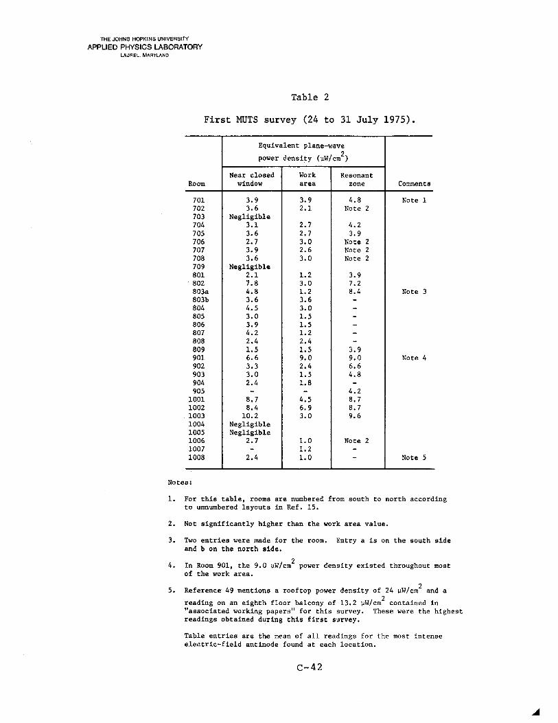
THE JOHNS HOPKINS UNIVERSITY
APPLIED PHYSICS LABORATORYLAUREL, MARYLAND
Table 2
First MUTS survey (24 to 31 July 1975).
Equivalent plane-wave2power aensity (~W/cm )
Near closed Work ResonantRoom window area zone Comments
701 3.9 3.9 4.8 Note 1702 3.6 2.1 Note 2703 Negligible704 3.1 2.7 4.2705 3.6 2.7 3.9706 2.7 3.0 Note 2707 3.9 2.6 Note 2708 3.6 3.0 Note 2709 Negligible801 2.1 1.2 3.9802 7.8 3.0 7.2803a 4.8 1.2 8.4 Note 3803b 3.6 3.6 -804 4.5 3.0 -805 3.0 1.5 -806 3.9 1.5 -807 4.2 1.2 -808 2.4 2.4 -809 1.5 1.5 3.9901 6.6 9.0 9.0 Note 4902 3.3 2.4 6.6903 3.0 1.5 4.8904 2.4 1.8 -905 - - 4.2
1001 8.7 4.5 8.71002 8.4 6.9 8.71003 10.2 3.0 9.61004 Negligible1005 Negligible1006 2.7 1.0 Note 21007 - 1.2 -1008 2.4 1.0 - Note 5
Notes:
1. For this table, rooms are numbered from south to north accordingto unnumbered layouts in Ref. 15.
2. Not significantly higher than the work area value.
3. Two entries were made for the room. Entry a is on the south sideand b on the north side.
4.
5.
2In Room 901, the 9.0 ~W/cm power density existed throughout mostof the work area.
2Reference 49 mentions a rooftop power density of 24 ~W/cm and a2reading on an eighth floor balcony of 13.2 ~W/cm contained in
"associated working papers" for this survey. These were the highestreadings obtained during this first survey.
Table entries are the mean of all readings for the most intenseelectric-field antinode found at each location.
C-42

THE JOHNS HOPKINS UNIVERSITY
APPLIED PHYSICS LABORATORYLAUREL, MARYLAND
unknown. Furthermore, its large size makes it unsuited to measurepower density in such a reflective environment. The intent was onlyto report received power and not power density. Instead of reading0.025 and 0.120 mW, the two MSR's read "mW/sqcm." This error wasnot noted and corrected until April 1976 (Ref. 49).
After the July survey, the lC probe for the energy densitymeter had been returned to the United States. A lB probe was received at the Embassy on 19 November 1975, but it proved to haveinsufficient sensitivity to measure the energy density within thebuilding. By the end of November, the lC probe had been returnedto the Embassy, and on 30 November 1975 the second energy densitysurvey began. No energy density or power density measurements weremade during the interval between these two surveys.
The second survey involved frequent measurements in manyoffice and apartment areas and was continued well into 1976 on analmost daily basis. By 8 February 1976, temporary screening hadbeen installed over all east- and south-facing windows and doors(Ref. 35). The entire installation took about five days. Sincepower density decreased to exceedingly low levels within the screenedrooms, the writer has chosen to consider only the data taken between30 November 1975 and 5 February 1976 (the midpoint of the installation) in establishing a power density model.
As in July, the lC probe was used to find antinodes (regionsof maximum electric field) around the windows and throughout theworking and living areas. During July, window area readings weretaken behind closed windows and with the probe extended out theopen window. Because of the multiple reflections involved and because of the more sheltered location of the probe when the windowwas closed, a significant difference was usually noted between antinode levels with the window opened and closed. Calculations haveshown (Appendix C) that the average transmission loss of the doubleglazed windows is only 0.7 dB. The two sets of readings do notserve to approximate window transmission loss, and the open windowmeasurements have little meaning. Initially, the second survey'sopen-window measurements were taken by extending the probe froma very slight opening in the window (it was winter-time!), andthis procedure did not allow a very effective search for a fieldmaximum. Subsequently, no open-window readings were taken at all.The open-window readings have been discarded from both surveys because a comparison is meaningless.
All antinode readings (from almost-daily telegrams too numerous to reference) were grouped according to room. For each room,
C-43

THE JOHNS HOPKINS UNIVERSITY
APPLIED PHYSICS LABORATORYLAUREL, MARYLAND
the closed-window and working-area readings were averaged and theirstandard deviations and extreme values found. These equivalentplane-wave power density values are shown for each location in Table3. Once again, these values refer to local field maximums. Theaverage power density throughout each room was probably about halfthe mean value listed under "working area." Rooms 1001 and 1002had the highest mean antinode intensities in the working area (3.7
2and 3.4 ~W/cm , respectively).
There are some isolated high values. The levels recordedduring a two-hour period on 24 February 1976 were unusually high.Measurements during this interval are shown as the extreme valuerecorded for many rooms in Table 3. The highest reading during
this interval was 24 ~W/cm2 in Room 1001. Excluding the readingstaken during this two-hour period, the highest reading inside the
building was 9.6 ~W/cm2 (slightly exceeded during the July survey).
Note footnote number 2 in Table 3 pertaining to Room 1003.This illustrates the uncertainty when inferring an equivalent planewave power density from the antinode reading of an electric-fieldenergy density meter. Because of the standing wave from the backof a safe placed against the window ledge, the maximum electricfield is twice that of the incident wave. As described earlier inthe report, this implies a quadrupling of power density. Based on
the highest equivalent power density reading of 42 ~W/cm2 in thissmall area, and also on the assumption that a standing wave existsdue to a single reflection, the power density of the incident wave
would have been about 10 ~W/cm2. If a second reflection (such as
one from the window frame) had contributed to the 42 ~W/cm2 reading,then the power density of the incident wave might have been evenlower. However, despite the uncertainty about power density, the
electric and magnetic fields corresponding to 42 ~W/cm2 (see Fig.1) did exist, but at different antinode locations in the standingwave. This small area above the window ledge would not have beenentered by anyone except for someone reaching behind the safe toplace something on the ledge.
The temporary screens that had been installed by 8 February1976 were replaced with permanent screens in May 1976. The newscreens covered all windows in the central building and in boththe north and south wings. The replacement was made on a room-byroom basis. While measurements continued to be recorded in the fewoffices with screens that could be swung open, the screens reducedthe fields within the rooms to very low levels.
C-44

THE JOHNS HOPKINS UNIVERSITY
APPLIED PHYSICS LABORATORYLAUREL, MARYLAND
Table 3
Second MUTS survey (30 November 1975 to 5 February 1976).
Equivalent plane-wave power density (~W/cm2)
Near Throughoutclosed window working area
Number of Standard Date of Standard Date ofRoom measurements Mean deviation Extreme Extreme Mean deviation Extreme extreme Comments
701 2 1.4 - 1.5 13 Dec 1.1 - 1.2 5 Dec702 2 1.8 - 2.4 14 Dec 1.4 - 1.8 14 Dec703 1 0.3 5 Dec704 3 1.5 0.8 2.4 14 Dec 0.9 0.3 1.2 14 Dec705 1 0.9 5 Dec 0.6 5 Dec707 1 0.6 5 Dec 0.6 5 Dec709 1 1.8 1 Dec 1.2 1 Dec801 5 3.4 1.2 5.4 3 Dec 1.3 1.3 3.0 24 Jan802 5 4.6 3.1 9.6 5 Dec 3.3 2.2 6.0 24 Jan803 3 3.5 1.8 4.8 3 Dec 1.0 0.7 1.8 3 Dec804 1 4.8 24 Jan 6.0 24 Jan805 3 2.4 0.6 3.0 30 Nov 1.5 1.1 2.4 30 Nov806 3 2.6 0.4 3.0 3 Dec 1.2 0 1.2807 5 2.4 0.6 3.0 3 Dec 1.3 1.0 2.4 24 Jan808 1 2.4 24 Jan 1.8 24 Jan809 4 1.6 0.6 2.4 24 Jan 1.1 0.9 2.4 24 Jan810 1 1.8 24 Jan 1.2 24 Jan
SS-8 6 0.8 0.4 1.2 1 Dec 0.8 - 1.2 6 Dec901-East 93 2.7 1.8 7.8 4 Dec Rm 901 readings merged below901-South 49 0.8 0.6 4.2 5 Dec 1.5 1.2 6.0 4 Dec
902 65 2.0 1.5 7.2 24 Jan 2.2 2.0 10.2 24 Jan Note 1903 32 2.0 1.0 4.0 24 Jan 1.8 1.3 7.2 24 Jan904 5 2.0 1.5 4.2 3 Dec 1.0 1.2 3.0 3 Dec
SS-9 6 2.7 1.3 4.2 16 Jan 1.2 0 1.21001 38 7.2 5.1 24.0 24 Jan 3.7 2.1 8.4 31 Dec1002 31 4.4 2.5 12.0 24 Jan 3.4 2.5 13.2 24 Jan1003 35 Note 2 3.0 2.2 11.4 24 Jan1005 3 1.4 0.9 2.4 10 Dec 0.9 0.8 1.8 10 Dec1006 15 2.0 1.1 3.6 3 Dec 1.1 0.5 1.8 24 Jan1007 1 0.6 5 Dec 1.2 Note 3 5 Dec1008 17 1.8 1.2 4.2 4 Dec 1.7 1.3 3.6 4 DecC5EL 2 0.6 - 0.9 15 DecS5CB 1 0.6 15 Dec 1.2 Note 4 15 DecS5CL 2 0.5 - 0.6 11 Dec 0.3S5CR 1 0.6 11 Dec 0.3 11 DecS6BK 3 0.7 0.2 0.9 15 Dec 0.9 0.9 1.5 15 DecS6BL 5 0.3 0.4 0.9 8 Dec 0.6 0.6 1.2 15 DecS6BB 3 0.8 0.2 0.9 15 Dec 0.6 0.5 1.2 15 DecS7AL 2 0 0S7BK 2 1.5 - 1.8 15 Dec 1.5 - 2.1 15 DecS7BB 2 1.4 - 1.5 15 Dec 1.6 - 2.1 15 DecS7BL 3 0.8 0.4 1.2 8 Dec 0.3NWR 1 Note 5 3.0 9 DecCWR 1 Note 5 13.2 to 9 Dec
15.0
Notes:
1. Many extreme values were recorded on 24 January 1976 during a period of MUTS-IA transmissions (0.5 to 2 GHz)between 4 snd 6 pm (maximum power was at 1.56 GHz).
2. Window area measurements ranged as high as 42.0 ~W/cm2 due to a standing wave from the back of a safe whichpartially blocks the window; this is not a work area.
3. Readings quoted as "low" were assumed to be O. 3 ~W/cm2, as per Ref. 34.
4. Apartment rooms designated in Ref. 50 as "room number called S6BB, S6BL. S6BK. 57BB, S7BL, S7BK, and S7ALrefer to south wing apa~tments. S6BB is the bedroom in Aparment 6B; S6BL is the living room of Apartment 6B;SCBK is the kitchen of Aparment 6B, etc." SS-8 and SS-9 refer to the southernmost stairways in the centralbuilding on the eighth and ninth floors.
5. For readings on the north wing roof (NWR) and the central wing roof (CWR), measurements were made as close tothe front of the building and as far south as practical.
Table entries are the mean of all readings for the most intense electric-field antinode found at each location.
C-45
THE JOHNS HOPKINS UNIVERSITY
APPLIED PHYSICS LABORATORYLAUREL, MARYLAND
In May 1976, a horn and power meter were used in an attemptto measure the levels within the rooms (Ref. 43). When held 1 footfrom the small gaps along the edges of the screen, a signal ranging
from 0.001 to 0.008 ~W/cm2 could be detected. Elsewhere within therooms, no meter movement was discerned except near the south-facingwindows in Rooms 901 and 1001. In those locations, during MUTS-2A
2operation (0.5 to 2 GHz), levels ranging from 0.001 to 0.002 ~W/cm
were read (the minimum perceptible signal on the meter). Becauseof the difficulties involved in measuring the energy leaking aroundthe edges of the screens, and also because of the problem of main-
2taining screen integrity, a higher level (0.1 ~W/cm ) is used inthe MUTS model.
In essence, because of the screening and the ensuing decreasein transmitted power, the microwave levels within the buildings maybe considered negligible at any time after 8 February 1976. The
signal incident on the building was about 2 ~W/cm2 after this time(Ref. 7); that would have been the exposure level for anyone working on the roof until the time defined as the end of the study (1February 1977).
MUTS MICROWAVE POWER DENSITY MODEL
Compared to the TUMS study, in which a variety of equipmentand techniques were used to measure power density within the building, the MUTS data is more detailed in form and more readily comparable. Other than the unsuccessful attempt in June 1975 to find apower density level within the building that would raise the indi-
cator on the Narda radiometer to its sensitivity limit of 10 ~W/cm2,only two sets of measurements were made prior to the time when thebuilding's windows and doors were screened. Both used the sameequipment, the same procedures, and essentially the same participants. One was made before the CW addition to the MUTS spectrumand the appearance of the MUTS-2 source, and the second survey wasperformed afterward.
Both surveys used the electric-field energy density meterwith the sensitive 1C probe. Window areas and working areasthroughout the rooms were probed and the highest fields recorded.These energy density values were converted to the power density ofan equivalent plane wave having the same electric field energy den-
2sity. No field was found above the 0.3 ~W/cm limit of the instru-ment in any room that did not have a window facing south or east(toward the transmitters). The results of these two surveys havebeen presented separately in Tables 2 and 3.
C-46

THE JOHNS HOPKINS UNIVERSITY
APPLIED PHYSICS LABORATORYLAUREL, MARYLAND
The average antinode intensities for the common region ofboth surveys are given in Table 4 and shown in Figs. 4 through 7.Figures 4 through 7 represent the east side of the building. Thegeneral increase in power level toward the upper southeast cornerof the building may be seen. Because this includes all the MUTSdata, these data represent the power density model for MUTS. Additional areas, with data available only from the second survey, arelisted in Table 3. Table 3 also contains standard deviation andextreme values to assist in estimating the variation of these intensities about the mean. In general, the similiarity between thetwo sets of entries in Table 4 is surprising, considering thechanges that took place in the time between them. (Of course onlyrooms 1001 and 901 and the stairway have windows facing south.)*
Several documents were found that expressed concern abouthigh field intensities occurring in the fall of 1975. This wasshown in the last section to have resulted from typographical errors in several monthly status reports. There are no MUTS powerdensity data for the interval prior to the installation of screensthat are not listed in Tables 2, 3, and 4. Therefore, there is noreason to believe that power levels were significantly differentfrom those averages shown in Table 4 for any significant period oftime. After all, these measurements were made only a half-yearapart. To help settle this issue, random sections of the stripcharts from the MUTS four-channel activity monitor were examined.October tracings were compared to those made during the July survey. Because of the cumbersome nature of this procedure, only asmall interval of the October tracing was examined, but there wasno significant difference between the apparent levels shown.
Accordingly, the writer proposes that the high field regionfor the MUTS model be as shown in Table 4 supplemented by thoseadditional areas described in Table 3. If additional nearby quarters have a southern or eastern window exposure comparable to thoselisted in Table 3, they should be included in this higher fieldregion. The levels within any such areas must be estimated fromthose listed in Table 3 subject to the general observation that thelevels appeared to decrease with distance from the southeast rooftop corner of the central building.
*According to Table 4, the most significant difference between thetwo surveys was in the Ambassador's office (room 901). Despitethe presence of MUTS-2 and the south-facing window in this room,the levels recorded during the second survey were much lower.Measurement personnel recall this difference and note that theonly change was a different arrangement of furnishings.
C-47

THE JOHNS HOPKINS UNIVERSITY
APPLIED PHYSICS LABORATORYLAUREL, MARYLAND
Table 4
MUTS microwave power density model.
2Mean equivalent plane-wave power density (~W/cm )
Location Ju1 1975 survey 30 Nov 1975 - 5 Feb 1976 survey
(room no.) Window area Work area Window area Work area
701 3.9 3.9 1.4 1.1702 3.6 2.1 1.8 1.4703 NR NR NR 0.3704 3.1 2.7 1.5 0.9705 3.6 2.7 0.9 0.6706 2.7 3.0 NR NR707 3.9 2.6 0.6 0.6708 3.6 3.0 NR NR709 NR NR 1.8 1.2801 2.1 1.2 3.4 1.3802 7.8 3.0 4.6 3.3803 4.2 2.4 3.5 1.0804 4.5 3.0 4.8 6.0805 3.0 1.5 2.4 1.5806 3.9 1.5 2.6 1.2807 4.2 1.2 2.4 1.3808 2.4 2.4 2.4 1.8809 1.5 1.5 1.6 1.1810 NR NR 1.8 1.2901 6.6 9.0 1.8 1.5902 3.3 2.4 2.0 2.2903 3.0 1.5 2.0 1.8904 2.4 1.8 2.0 1.0905 NR NR NR NR
1001 8.7 4.5 7.2 3.71002 8.4 6.9 4.4 3.41003 10.2 3.0 SW 3.01004 NR NR NR NR1005 NR NR 1.4 0.91006 2.7 1.0 2.0 1.11007 NR 1.2 0.6 1.21008 2.4 1.0 1.8 1.7
Rooftop* - 24.0 - 15.0
Notes:
*Rooftop measurements are the highest readings found with the few measurementsmade; they are reported to have been made at an unusually intense reflectiveantinode.
NR indicates not recorded
SW indicates standing wave
C-48

",
() I ,j:>,
1.0
RO
OFT
OP*
24.0
1001
1002
1003
1004
1005
1006
1007
1008
8.7
8.4
10.2
NR
NR2.
7NR
2.4
901
902
903
904
905
6.6
3.3
3.0
2.4
NR
801
802
803
804
805
806
807
808
809
810
2.1
7.8
4.2
4.5
3.0
3.9
4.2
2.4
1.5
NR
701
702
703
704
705
706
707
708
709
3.9
3.6
NR3.
13.
62.
73.
93.
6NR
Key
:N
R-
not
reco
rded
Bol
dfac
enu
mbe
rsar
ero
omnu
mbe
rs.
Thi
sre
pres
ents
ast
yliz
eddi
agra
mof
the
east
side
of
the
Em
bass
y;it
isno
tto
scal
e.T
henu
mbe
rsbe
low
the
room
num
bers
are
the
mea
neq
uiva
lent
plan
e-w
ave
pow
erde
nsit
yin
pW/c
m2
.
*The
roof
top
valu
eis
not
the
aver
age,
but
isth
ehi
ghes
tre
adin
gfo
und
ofth
efe
wm
easu
rem
ents
mad
e;it
was
said
tobe
atan
unus
uall
yin
tens
ere
flec
tive
anti
node
.
Fig.
4M
UT
Sm
icro
wav
epo
wer
dens
ity
mod
el-
mea
neq
uiva
lent
plan
e-w
ave
pow
erde
nsit
y,Ju
ly19
75su
rvey
,w
indo
war
eas.
~ "...
cff
im
<- °0,....,,~
~:I:Cf)
"'-<:
I:j!!~~
~o~
>C
f)z
:2r
cn>)>o~
~~;ii
:Dill
~~ ~
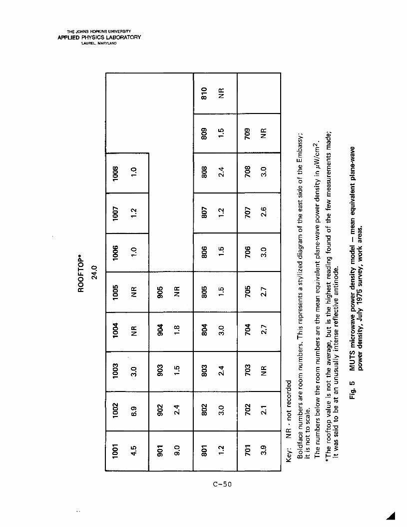
~
n I \J1 a
RO
OF
TO
P*
24.0
1001
1002
1003
1004
1005
1006
1007
1008
4.5
6.9
3.0
NRN
R1.
01.
21.
0
901
902
903
904
905
9.0
2.4
1.5
1.8
NR
801
802
803
804
805
806
807
808
809
810
1.2
3.0
2.4
3.0
1.5
1.5
1.2
2.4
1.5
NR
701
702
703
704
705
706
707
708
709
3.9
2.1
NR2.
72.
73.
02.
63.
0N
R
Key
:N
R-
no
tre
cord
ed
Bol
dfac
enu
mbe
rsar
ero
omnu
mbe
rs.
Thi
sre
pres
ents
ast
yliz
eddi
agra
mof
the
east
side
of
the
Em
bass
y;it
isno
tto
scal
e.T
henu
mbe
rsbe
low
the
room
num
bers
are
the
mea
neq
uiva
lent
plan
e-w
ave
pow
erde
nsit
yin
IlW
/cm
2.
*The
roof
top
valu
eis
no
tth
eav
erag
e,b
ut
isth
ehi
ghes
tre
adin
gfo
und
of
the
few
mea
sure
men
tsm
ade;
itw
assa
idto
beat
anun
usua
lly
inte
nse
refl
ecti
vean
tino
de.
Fig.
5M
UT
Sm
icro
wav
epo
wer
dens
itym
odel
-m
ean
equi
vale
ntpl
ane-
wav
epo
wer
dens
ity,
July
1975
surv
ey,
wor
kar
eas.
~ "tl
....cff
im
...C
or;"tl~
c:I
:cn
"-(:1
:f!~~
;c:o~
~cn~
~>c
Zm~
oo.
rii:IJ~
~~ ~

,.
() I U1 ......
RO
OFT
OP*
15.0
1001
1002
1003
1004
1005
1006
1007
1008
7.2
4.4
SWNR
1.4
2.0
0.6
1.8
901
902
903
904
905
1.8
2.0
2.0
2.0
NR
801
802
80
380
480
580
680
78
08
809
81
0
3.4
4.6
3.5
4.8
2.4
2.6
2.4
2.4
1.6
1.8
701
702
703
704
705
706
707
70
870
9
1.4
1.8
NR1.
50.
9NR
0.6
NR
1.8
Key
:N
R-
not
reco
rded
,SW
-st
andi
ngw
ave.
Bol
dfac
enu
mbe
rsar
ero
omnu
mbe
rs.T
his
repr
esen
tsa
styl
ized
diag
ram
ofth
eea
stsi
deo
fth
eE
mba
ssy;
itis
not
tosc
ale.
The
num
bers
belo
wth
ero
omnu
mbe
rsar
eth
em
ean
equi
vale
ntpl
ane-
wav
epo
wer
dens
ity
inJi
W/c
m2
.
*The
roof
top
valu
eis
not
the
aver
age,
but
isth
ehi
ghes
tre
adin
gfo
und
of
the
few
mea
sure
men
tsm
ade;
itw
assa
idto
beat
anun
usua
lly
inte
nse
refl
ecti
vean
tino
de.
Fig.
6M
UT
Sm
icro
wav
epo
wer
dens
ity
mod
el-
mea
neq
uiva
lent
plan
e-w
ave
pow
erde
nsit
y,3
0N
ovem
ber
1975
to5
Feb
ruar
y19
76su
rvey
,w
indo
war
eas.
~ "...
cff
im
e..
°0r,,~
~::I:(IJ
"-<
:I:
¥!~!
il;::()~
~cn~
~S;~
a~~
:Dil
l~~
o .:D -<

~
() I LT1
IV
RO
OFT
OP*
15.0
1001
1002
1003
1004
1005
1006
1007
1008
3.7
3.4
3.0
NR
0.9
1.1
1.2
1.7
901
902
903
904
905
1.5
2.2
1.8
1.0
NR
801
802
803
804
805
806
807
808
809
810
1.3
3.3
1.0
6.0
1.5
1.2
1.3
1.8
1.1
1.2
701
702
703
704
705
706
707
708
709
1.1
1.4
0.3
0.9
0.6
NR
0.6
NR
1.2
Key
:N
R-
no
tre
cord
ed
Bol
dfac
enu
mbe
rsar
ero
omnu
mbe
rs.
Thi
sre
pres
ents
ast
yliz
eddi
agra
mof
the
east
side
of
the
Em
bass
y;it
isn
ot
tosc
ale.
The
num
bers
belo
wth
ero
omnu
mbe
rsar
eth
em
ean
equi
vale
ntpl
ane-
wav
epo
wer
dens
ity
inpW
/cm
2.
*The
roof
top
valu
eis
no
tth
eav
erag
e,b
ut
isth
ehi
ghes
tre
adin
gfo
und
of
the
few
mea
sure
men
tsm
ade;
itw
assa
idto
beat
anun
usua
lly
inte
nse
refl
ecti
vean
tino
de.
Fig.
7M
UTS
mic
row
ave
pow
erde
nsity
mod
el-
mea
neq
uiva
lent
plan
e-w
ave
pow
erde
nsity
,30
Nov
embe
r19
75to
5Fe
brua
ry19
76su
rvey
,w
ork
area
s.
~ "tJ
....C
ffim
e..
Co
r;"tJ~
c::
:I:C
Il"-(J:
J!!~~
;:o~
>cn
z~
r.CI
l>
l>C
ZlJl~
co
rii
::o~
~~
o ~

THE JOHNS HOPKINS UNIVERSITY
APPLIED PHYSICS LABORATORYLAUREL, MARYLAND
The window area antinode intensities (Table 4), as for TUMS,are within 2 feet of either windows or glassed doors. The averagevalues throughout the room can be assumed to be half the workingarea antinode values.
The typical power density for rooms elsewhere in the central
building and wings can be assumed to be less than 0.1 ~W/cm2, as inTUMS, although a few rooms on the east side of the north wing areanearest to the central building may have had levels of 0.2 to 0.5
~W/cm2. This initial MUTS model covers the period from 28 May 1975(date of turn-on) until 5 February 1976 (midpoint of the period ofinstallation of temporary screens).
The second MUTS model covers the period from 6 February 1976to 1 February 1977 (the date of the end of this study). Because ofboth the screening and the transmitter power reductions, the highestlevels subsequently recorded within the building were less than
20.008 ~W/cm. However, because of the poor spatial resolution ofthe horn antenna and the difficulties involved in its use in measuring energy leaking around the screens, the writer believes ahigher value should be used in the MUTS model. Accordingly, a level
of 0.1 ~W/cm2 or less is assigned to all rooms within the building.This assumes a total reduction by a factor of 100 from the highestoffice value recorded in Table 4. The level on the rooftop is
22 ~W/cm throughout this second interval, as discussed in the pre-ceding section.
The difference between direct power density measurements andequivalent values obtained through the conversion of energy densitydata was discussed earlier. Figure 1 can be used in either case tofind the level of the E and H fields. For the direct measurement,as for TUMS, the E and H fields are those at the point of measurement and they are in phase. For the equivalent case, including allthe MUTS data, the indicated E and H fields are maxima which occurat separate, but perhaps nearby, locations. They are also not necessarily in phase. The true power density at the point of measurement is less than the equivalent value (at an antinode) due to theeffect of reflections, but the amount of this difference is unknown.
C-53


THE JOHNS HOPKINS UNIVERSITY
APPLIED PHYSICS LABORATORYLAUREL, MARYLAND
REFERENCES*
1. J. C. Slater and N. H. Frank, Electromagnetism, McGraw-Hill,Chapter 8.
2. P. F. Wacker and R. R. Bowman, "Quantifying Hazardous Electromagnetic Fields: Scientific Basis and Practical Consideration,"IEEE Trans. Microwave Theory and Techniques, Vol. MTT-19, No.2,Feb 1971.
3. "American National Standard Safety Level of ElectromagneticRadiation in Respect to Personnel," ANSI C95.l-l974.
4. J. A. Stratton, Electromagnetic Theory, McGraw-Hill, Section9.2.
5. B. R. Moore, "Is the Homing Pigeon's Map Geomagnetic?" Nature,Vol. 285, 8 May 1980.
6. H. P. Schwann and K. R. Foster, "RF Field Interactions withBiological Systems: Electrical Properties and BiophysicalMechanisms," Proc. IEEE, Vol. 68, No.1, Jan 1980, pp 104-113.
7. Statement by Herbert Pollack before the Committee on Commerce,Science, and Transportation, United States Senate, 27 Jun 1977.
8. Department of State Official Informal memo from Maclyn Musserto Elmer Hill, 22 Nov 1963.
9. "First Interim Progress Report - TUMS Program," Department ofState, 25 Mar 1966.
10. Letter from Charles Weiss to Col. Joseph Brady, 15 Feb 1967(Vol. I of the Freedom of Information Act folders).
11. Department of State Official Informal memo from Theodore Veato Chief, Department of Technical Services, 9 Oct 1967.
12. Department of State Official Informal memo from Theodore Veato Chief, Department of Technical Services, 16 Oct 1967.
*State Department telegrams are referenced by the place of originfollowed by the year and the sequence number within that year.
C-55

THE JOHNS HOPKINS UNIVERSITY
APPLIED PHYSICS LABORATORYLAUREL, MARYLAND
13. Memo from Theodore Vea to Technical Surveillance Countermeasures Committee USIB, 9 June 1969.
14. D. B. Staake, "RF Field Measurements, SPG-55B, in Buildings8 and 9," APL/ JHU F30-80-717, 2 Apr 1980.
15. "Investigation of the Potential Health Hazard to Staff of theU.S. Embassy Moscow from Extended Exposure to the MUTS Signal,"Department of State Memorandum for the Record, 1 Aug 1975.
16. Department of State Official Informal memo from LlewellynThompson to George Mishtoute, 20 Nov 1967.
17. Department of State Official Informal memo from Theodore Veato Robert Thomas, 15 Jun 1971.
18. Department of State Memo from SO(T) Moscow to Maclyn Musser,10 Feb 1972.
19. Department of State Official Informal memo from Theodore Veato Maclyn Musser, 3 Nov 1965.
20. Technical Report (TUMS) - TR001, 1966.
21. Letter from Theodore Vea to Weiss, Moscow 5567, 26 Jun 1967.
22. Letter from Donovan Fischer to K. W. Knauf, 3 May 1972 (itemNo. 67, Vol. 2 of the Freedom of Information Act folders).
23. Department of State Official Informal memo from Theodore Veato Chief, Division of Technical Services, 18 May 1967.
24. Department of State Official Informal memo from Theodore Veato Chief, Division of Technical Services, 25 Sep 1967.
25. "Plantenna Gives Horn Performance in 3/4-in. Depth," Microwaves, May 1963, pp 84-85.
26. Department of State Official Informal memo from Theodore Veato Chief, Division of Technical Services, 5 Oct 1967.
27. F. Perra, "Project SMUT Report" 1 July 1972 (item No. 72, Vol.2 of the Freedom of Information Act folders).
28. Department of State Moscow telegram 75-08918.
29. Department of State Monthly Status Report, Moscow Embassy,May 1975.
C-56

THE JOHNS HOPKINS UNIVERSITY
APPLIED PHYSICS LABORATORYLAUREL, MARYLAND
30. Department of State Monthly Status Report, Moscow Embassy,Jun 1975.
31. Penciled notes in the front of the "MUTS: 1 May 76 tofolder in Department of State files.
"
32. Department of State Monthly Status Report, Moscow Embassy,Aug 1975.
33. Department of State Monthly Status Report, Moscow Embassy,Oct 1975.
34. Department of State Moscow telegram 76-00024.
35. Department of State Moscow telegram 76-01849.
36. Personal interview with F. Brandt, 22 Apr 1980.
37. Department of State Moscow telegram 76-01970.
38. Department of State Moscow telegram 76-02164.
39. Department of State Moscow telegram 76-02258.
40. Department of State Moscow telegram 76-03798.
41. Department of State Moscow telegram 76-06814.
42. Department of State Moscow telegram 76-13251.
43. Department of State Monthly Status Report, Moscow Embassy,May 1976.
44. Department of State Monthly Status Report, Moscow Embassy,Jun 1976.
45. Department of State Moscow telegram 76-17615.
46. Department of State Monthly Status Report, Moscow Embassy,Ju1 1975.
47. Memo from Lawrence Eag1eburger to Victor Dikeos through JohnThomas, 10 Dec 1975.
48. Department of State Moscow telegram 75-18375.
49. Department of State Moscow telegram 76-06706.
C-57
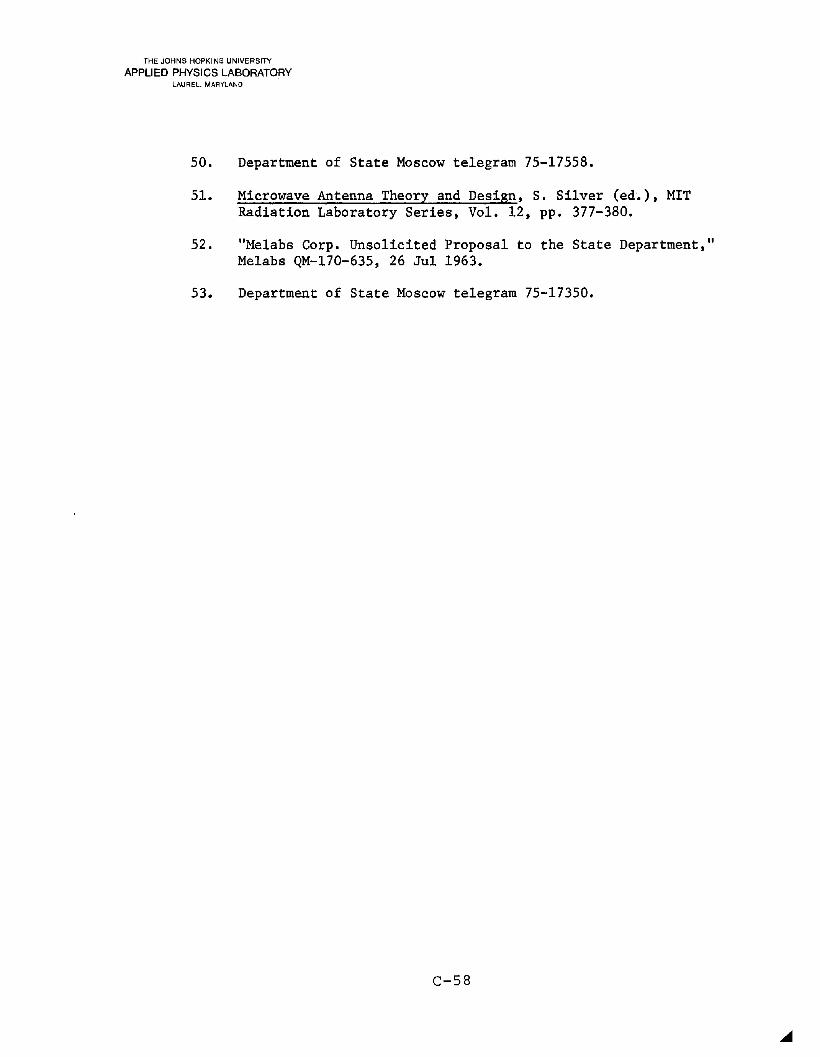
THE JOHNS HOPKINS UNIVERSITY
APPLIED PHYSICS LABORATORYLAUREL, MARYLAND
50. Department of State Moscow telegram 75-17558.
51. Microwave Antenna Theory and Design, S. Silver (ed'.), MITRadiation Laboratory Series, Vol. 12, pp. 377-380.
52. "Me1abs Corp. Unsolicited Proposal to the State Department,"Me1abs QM-170-635, 26 Ju1 1963.
53. Department of State Moscow telegram 75-17350.
C-58

THE JOHNS HOPKINS UNIVERSITY
APPLIED PHYSICS LABORATORYLAUREL, MARYLAND
Appendix A
A DESCRIPTION OF THE ANTENNAS USED
If an antenna is positioned to receive the maximum signalfrom a single-frequency radio wave of matched polarization, thereceived power may be calculated from:
(A-I)
where PD is the incident power density and Aeff is the effective
receiving area of the antenna. All antennas have an effective areaeven if their physical cross section is negligible (such as a whipor long-wire antenna). Effective area is not directly measurable,but is derived from the antenna's gain. Gain is a measure of therelative concentration of an antenna's beam. This value (a ratio)is measured directly by comparing the signal level received by theantenna to that received by a calibrated "standard gain" antenna.This comparison is made at one frequency at a time across the bandwidth of interest. Effective area is then calculated from antennagain (expressed as a power ratio) as follows:
where A is the wavelength. This equation is valid for any type ofantenna.
To calculate incident power density, Eq. A-I may be rearranged as
The received power is measured and then divided by the antenna'seffective area to determine the power density. For a broadbandsignal, the calculation should be done bit by bit across the frequency band, because effective area varies with frequency. Thisprocedure was followed when the spectral distribution of TUMS wasknown at the time of measurement. Usually, the spectral distribution was not known, and power density was determined by using the
C-59
THE JOHNS HOPKINS UNIVERSITY
APPLIED PHYSICS LABORATORYLAUREL, MARYLAND
average antenna effective area across the band. This uncertaintyis not significant unless the energy was concentrated near one endof the band, and there is no evidence that this occurred.
Two antennas were used for TUMS power density measurements.The first, a Po1arad CA-S antenna, is a linearly polarized microwave horn. Its gain is shown in Fig. A-1 (from Ref. 20), and thederived effective area is plotted in Fig. A-2 (including a smallcorrection to the plotted data). The corrected values were usedin the report. Calculated beamwidth is plotted in Fig. A-3.
The second antenna, the Aero-Geo-Astro Corporation's ModelPWR-284 P1antenna is also linearly polarized, but of a more unusualdesign (Ref. 25). A relatively thin antenna with a moderate gainwas devised by mounting a dipole feed in a shallow covered cavityand surrounding it with a small groundp1ane. This is in essence a"box-horn" design (Ref. 51) in which the cavity depth is adjustedto achieve an in-phase condition between the first and third waveguide modes at the aperture. This flattens the amplitude distribution across the aperture and increases gain. References 25 and 52indicate that the gain of the P1antenna is relatively constant(approximately 9 dB) across the TUMS band. Using this value, theeffective area was calculated and plotted in Fig. A-4. Half-powerbeamwidth is approximately 63° across the band.
When the level of the MUTS signal was reduced in February1976, the sensitivity of the EDM-1C energy density meter was insufficient to record the signal even when the window screens wereopened. For the measurements to continue, the more sensitive combination of a horn and power meter was required.
Before this happened, a series of measurements had been takento compare the equivalent power density of the EDM-1C to that measured directly at the same point by the combination of a horn andpower meter. Empirical adjustment factors were derived from thismeasurement sequence (Ref. 53) to adjust upward the direct powerdensity reading of the horn to approximate the equivalent value derived from the reading of the energy density meter. These adjustment factors compensate for two gross differences. First, even whenthe horn is rotated to maximize its signal, there are two remainingpolarization components to which it remains insensitive. The seconddifference is that in the presence of reflections, the equivalentpower density is greater than the direct power density if the equivalent reading is taken in an antinode.
These adjustment factors were 1.15 for band A (0.5 to 2 GHz)and 2.1 for band B (2 to 4 GHz). This procedure was used only for
C-60
THE JOHNS HOPKINS UNIVERSITY
APPLIED PHYSICS LABORATORYLAUREL, MARYLAND
MUTS and only after the temporary screens had been installed (8February 1976). The horn used was the Sylvania AN-lOB. Its gainand calculated effective area are shown in Figs. A-5 and A-6, respectively. The effective area curve for the Sylvania horn (Fig.A-6) is more irregular than the smooth curves shown for the CA-Shorn (Fig. A-2). This is due to the more complex feed requiredfor this broadband horn.
C-61

THE JOHNS HOPKINS UNIVERSITY
APPLIED PHYSICS LABORATORYLAUREL, MARYLAND
4.54.03.53.02.52.01.5
21 r------,-----,.----,----~---_r_---r_--___,
19
16
14 '--- J- .L...- J- L...-.__---JL...-.__---I --J
1.0
17
18
15
20
Frequency (GHz)
Fig. A-1 Gain versus frequency for Polarad model CA-S antenna.
C-62

THE JOHNS HOPKINS UNIVERSITY
APPLIED PHYSICS LABORATORYLAUREL, MARYLAND
580 r----,------,----,------,----,----...,..----,
~560 \
\
"\540 \\\"-520 \
\\
500 "N \E(.)- \ctIC1l... 480 "-ctI
C1l
\>'';::::;(.)
\C1l'+-'+-UJ ,
460 ,",
440 ""420
400Note: ---Corrected according to
gain curve (A = GX2/41T)
4.54.03.53.02.52.01.5
380L-__--L ....L- L--__--L ....L- L--__---'
1.0
Frequency (GHz)
Fig. A-2 Effective area versus frequency for Polarad model CA-S antenna.
C-63

THE JOHNS HOPKINS UNIVERSITY
APPLIED PHYSICS LABORATORYLAUREL, MARYLAND
30~------r-------..-------r--------,
W- ~ 32,000B --G
25
C;;Q)
::£.I;+-'"0.~
EctlQ) 20.0...Q)
s:0c.~"'i6:::c
15
4.54.03.5Frequency (GHz)
3.0
10 '--- --L. ..l..---,- --L ...I
2.5
Fig. A·3 Calculated beamwidth of Polarad model CA·S antenna.
C-64

THE JOHNS HOPKINS UNIVERSITY
APPLIED PHYSICS LABORATORYLAUREL, MARYLAND
90 r------,--------,.--------r--------,
G }.2A=-
47T
80
70
('II
E~
coQ)~
co 60~
.';:;()
~'+w
50
40
4.54.03.0 3.5
Frequency (GHz)
Fig. A·4 Calculated effectiv~ area of Plantenna.
30 L..- ..L.- ....L- --I- --1
2.5
C-65

THE JOHNS HOPKINS UNIVERSITY
APPLIED PHYSICS LABORATORYLAUREL, MARYLAND
~..../
....
//(
00
\,\ ~
\ 0 00; CO
"\ 0, ciij
I '0::
\ 0 CIl
cx5 ~
c,~
0
\ .c"t:l\ c
\ 0 N CO:r: .c
" "t:l
I <.9 CO0
J> ~
(,) .cc I:Q
IQ)
0::J0 0- ....
~I
(0Q) :2:....
LL. «\ ....\ 0
>,(,)
\ 0cCIl
\ LO ::s0-
\ CIl~...., en::s, en~
\ 0CIl>
o::i c, '(6, 0,,LO
I
\.. ~ «"
M,~,LL.
'a,, 0N
\\..
LO 0 LO 0 LO 0N N .... ....
(SP) u!e8
- 66

THE JOHNS HOPKINS UNIVERSITY
APPLIED PHYSICS LABORATORYLAUREL, MARYLAND
200r------,-----r-----.-------r-------r---------.
GX2A=-
41T160
NE 1202eoQ)....eoQ)
>'';:;uQ)
80"l-"l-UJ
40
121086
Frequency (GHz)
420'-------'-------'-------'-------'-------'---------'
o
Fig. A-6 Calculated effective area of AN-10B horn.
C-67

THE JOHNS HOPKINS UNIVERSITY
APPLIED PHYSICS LABORATORYLAUREL, MARYLAND
Appendix B
THE EDM-IC ENERGY DENSITY METER
A straight-wire dipole antenna responds to RF electromagneticfields in which the electric field has a component parallel to thedipole. If the dipole length is one-half wavelength or less, theintensity of its beam (in terms of the electric field strength) isproportional to the sine of the angle from its axis. It is therefore a wide-beam antenna, isotropic in one plane, with a beam shapethat remains the same for any frequency where the dipole is no longerthan one-half wavelength. If the received voltage of the electrically short dipole is detected by a diode operating in its squarelaw region, the output current is proportional to the energy contained in one of the three mutually independent electric-field components. If three such dipoles and detectors are oriented perpendicular to each other so that they cross at the center of each dipole (which calls for very ingenious packaging) and the three outputs are summed, the instrument can be calibrated to read totalelectric-field energy density (summing the energy of all three orthogonal electric field components, despite their relative phasing)at the location of the probe. The output will be independent ofthe orientation of the probe at that point and, in addition, thedevice sums the electric-field energy density at all frequencieswithin its band of operation. The probe is insensitive to the RFmagnetic field components.
The National Bureau of Standard EDM-lC energy density meteris such a device. It was devised for use in microwave hazard surveys (Ref. 2). The basic meter (EDM) may be fitted with differentprobes. The lC probe was the more sensitive of the two availableduring this survey (the lB was used without success in November1975 because of its lack of sensitivity). The device reads thetotal energy density of the electric field in fractions of a jouleper cubic meter. To convert to the equivalent power density of aplane wave with an identical electric field strength, the readingis multiplied by 2 to account for the equal magnetic-field energydensity at any point in a plane wave. The resulting product ismultiplied by the speed of light to convert to watts per squaremeter, and then multiplied by 100 to convert to microwatts persquare centimeter. This conversion is rigorous only for a planewave, since in a multipath environment the proportion of electricfield to magnetic-field energy will vary from point to point.
C-68
THE JOHNS HOPKINS UNIVERSITY
APPLIED PHYSICS LABORATORYLAUREL, MARYLAND
The device is calibrated for any microwave frequency up to3 GHz (most MUTS energy was below 3 GHz). Above that frequency,the device will respond, but its directionless quality (and therefore calibration) is lost because the dipole beam shapes becomemore complex. The sensitivity of the probe is stated at different
values in various documents but it probably is about 0.6 ~W/cm2equivalent plane-wave power density, with a meter response at levels
as low as 0.3 ~W/cm2.
C-69
THE JOHNS HOPKINS UNIVERSITY
APPLIED PHYSICS LABORATORYLAUREL, MARYLAND
Appendix C
WINDOW INSERTION LOSS CALCULATIONS
During the evaluation of the variety of TUMS measurements,it became desirable to be able to compare data taken within theTUMS observation room to those taken elsewhere within the Embassy.While all Embassy windows were double-glazed as a thermal insulation technique (independent inner and outer windows separated byabout three inches), the inner glass window in the observation roomhad been replaced by a sheet of quarter-inch plywood. Since essentially all microwave energy enters these rooms through the windows,we needed to determine if the window insertion loss for the TUMSobservation room was significantly different from the other rooms.
To answer this question, a loss calculation was made usinga computer program written to compute both the transmission and reflection for a plane wave incident on a large, flat, multilayerstructure. This program had been written initially to analyze transmission through radomes (covers enclosing radar antennas). Itsvalidity has been established by comparing its predictions to alarge variety of comparison data involving materials as diverse asplastics, ceramics, water, and thin layers of metal.
While relatively insensitive to small errors in the thickness of the glass panes (these effects would show up at higher frequencies or at high angles of incidence), an error in the largerdimension of the air separation between panes could bias the calculation over this limited bandwidth. To avoid this, the air spacedimension was purposely set to a value high enough to obtain severalfull reflection cycles, thus allowing a more accurate evaluation.
As frequency increases, transmission through either windowwill go through a series of cycles as the various reflections addconstructively or destructively. Figure C-l shows power transmission versus frequency for two one-eighth inch glass panes with eightinch spacing. A dielectric constant of 4.5 (typical for glass) wasused with a zero loss tangent* (actually the loss tangent for glassis small but finite; if it were included, it would have caused the
*See Appendix D for a definition of dielectric constant and losstangent.
C-70

THE JOHNS HOPKINS UNIVERSITY
APPLIED PHYSICS LABORATORYLAUREL, MARYLAND
maximums to slowly fall away from the unity transmission line).The effect of the reflections going in and out of phase is easilyseen. Figure C-2 shows the same calculation for the TUMS observation window with the plywood inner layer. Tabulated electricalconstants for plywood were used (€ = 1.5, tan 0 = 0.022).
r
In both cases, an average insertion loss was calculated byaveraging data in each figure over an integral number of reflectioncycles. When this was done, the average loss of the conventionalwindows was 0.7 dB, as compared to 0.5 dB for the TUMS window. Thedifference is trivial. This simi1iarity in average loss can be seenby overlaying the two figures.
In summary, the insertion loss of the two window configurations is nearly the same, so that power density measurements takenwithin the TUMS observation room may be considered typical of thelevels existing in nearby rooms.
Notes:Normal incidence
1/8" glass8" air space
1/8" glass
0.4
0.8
1.0 r---------r--:=-;:-----r--~r_-_._...-_r____""JI.,__-r___,
0.2
...~ 0.6o0-Q)
>'';:;coQ)
0:
OL- --L. -J.- "--__L.-_--L.._--L.-:----L----'
1 2 3 4 5
Frequency (GHz)
Fig. C-1 Relative power transmitted through window.
C-71

0.4
THE JOHNS HOPKINS UNIVERSITY
APPLIED PHYSICS LABORATORYLAUREL, MARYLAND
1.0 r--------~---_r_--__,_--...,....__-__,_-__,_-..,_____,
0.8
a..~ 0.6oQ.
~',j:;;co(ija:
0.2
Notes:Normal incidence1/8" glass
8" air space1/4" plywood
O'----------.J'--------'--__--L.__---'-__...L-_-'-_-'----J
1 2 3 4 5
Frequency (GHz)
Fig. C-2 Relative power transmitted through observation window.
C-72

Aattachednitude.
THE JOHNS HOPKINS UNIVERSITY
APPLIED PHYSICS LABORATORYLAUREL, MARYLAND
Appendix D
UNITS AND SOME PHYSICAL CONSTANTS
standard system of notation is used in which a prefix isto the basic unit of measurement to indicate relative magThese prefixes and their magnitudes are listed below. The
6magnitudes are in scientific notation in which 10 means a one fol-
lowed by six zeroes (one million) and 10-6 means the reciprocal(one millionth).
Prefix Symbol Magnitude
tera T 1012
giga G 109
mega M 106
kilo k 103
hecto h 102
deka da 101
deci d 10-1
centi c 10-2
milli m 10-3
micro 11 10-6
nano n 10-9
pico p 10-12
femto f 10-15
atto a 10-18
Using this notation, the unit of power density used in the text,2the microwatt per square centimeter (11W/cm ), is one-millionth of
a watt per square centimeter. The energy density unit, the pico3joule per cubic centimeter (pJ/cm ) is one-trillionth of a joule
per cubic centimeter.
C-73

THE JOHNS HOPKINS UNIVERSITY
APPLIED PHYSICS LABORATORYLAUREL, MARYLAND
The unit of frequency is the hertz (Hz), and is defined asone cycle per second. A typical microwave frequency of 3 GHz isthus three billion hertz.
A simple example may be used to gain an idea of the magnitudeof these power density quantities. One watt of power is defined asan energy flow of one joule per second. A 100 W light bulb converts100 J/s of electric energy into electromagnetic radiation (light and
2infrared). Since the surface area of the bulb is about 70 cm , the
power density on its surface is 1.4 W/cm2• According to the inversesquare law, ignoring any absorption by the intervening air, the power
2density 10 feet from the bulb is 86 ~W/cm. Fifty feet away, the
power density has decreased to 3.4 ~W/cm2. This is similar in magnitude to the power densities described in this report.
Another unit used in the text is the dBm/m2 • This again ispower density but it is referred to a square meter rather than asquare centimeter. The power portion of the notation (dBm) is decibels referred to one milliwatt (the decibel was discussed earlier).
A power density of -3 dBm/m2 is 0.5 mW/m2 •
The symbols € and ~ were used without definition in earlierequations. In this case, the symbol ~ is not a prefix; it has adifferent usage. These two symbols are constants of proportionalitythat appear in the basic electric and magnetic force equations. Asrequired by the system of units used (the rationalized MKS system)they are not unity even to characterize these forces in a vacuum.For a particular material these constants are:
(permitivity)
and
(permeability)
in which
farads/meter
and
C-74
THE JOHNS HOPKINS UNIVERSITY
APPLIED PHYSICS LABORATORYLAUREL, MARYLAND
11 0 henrys/meter
are the constants of free space or vacuum. The relative constantsE and 11 describe the characteristics of the particular material.
r rFor many materials, E and 11 may be represented by single realr rnumbers. If the material absorbs energy from alternating electricand magnetic fields, the relative constants are complex numbers.If the material has different properties along different axes, therelative constants are tensors. Crystal calcite has a tensor permitivity at optical frequencies. This accounts for the phenomenaof double refraction, whereby two displaced images are seen if onelooks through the crystal. The relative permitivity is usuallycalled the material's dielectric constant. If the material is absorbent, and its dielectric constant is complex, the ratio of itsimaginary to its real part is called the material's loss tangent(tan 8). These constants are used to calculate the reflection fromand transmission into material objects.
C-75

THE JOHNS HOPKINS UNIVERSITY
APPLIED PHYSICS LABORATORYLAUREL. MARYLAND
Appendix E
SUMMARY TIME CHARTS OF TRANSMITTER OPERATING HOURS
For both TUMS and MUTS, activity monitors were constructedto automatically record intervals of transmitter activity on acontinuous strip-chart recording. For a number of years, Embassypersonnel summarized the information on these traces by re-plottingit in the form of monthly summary charts. For this study, the summary charts were analyzed to determine the percent of the time thatthe transmitter was radiating (a) during the work day as comparedto the morning and evening hours, and (b) during the work week ascompared to the weekend. This was done by a combination of manualand computer data sorting. The duration of each interval of transmission, rounded off to the nearest half hour, was tabulated according to its time of occurrence during the day, the day of the week,the month, and the year. The daily time of occurrence was dividedinto three intervals: midnight to 8 a.m., 8 a.m. to 5 p.m., and5 p.m. to midnight. This table of data was then read into a desktop computer for further sorting and processing. As an example,the midnight to 8 a.m. bar in Fig. E-l was obtained by entering theend dates of the interval of interest. The data file was searchedfor all midnight to 8 a.m. entries between the two dates, theirdurations were totaled, and the sum was divided by the total midnight to 8 a.m. hours in the interval. This result is plotted as"percent of time the signal was recorded." The other bars wereobtained by a similar sorting procedure.
Figure E-l shows three breakdowns of TUMS activity for theperiod 1 February 1966 to 31 December 1970. Monitoring data forthe remaining TUMS interval (up to 26 May 1975) had been summarizedfrom the original strip charts but the corresponding summary chartscould not be found. At the top of Fig. E-l, signal activity isbroken down into three periods of the day, so as to show differencesin signal activity between the normal work day (8 a.m. to 5 p.m.)and other periods. The middle graph of Fig. E-l compares signalactivity during the normal work week (Monday to Friday) with thatfor weekends. The graph at the bottom of Fig. E-l compares TUMSactivity during the summer months with that for the remainder ofthe year.
The MUTS interval was divided into three parts. The firstbegins on 1 July 1975 (when monitoring started) and ends on 15 October 1975 (the day prior to the initial operation of MUTS-2). The
C-76

THE JOHNS HOPKINS UNIVERSITY
APPLIED PHYSICS LABORATORYLAUREL, MARYLAND
second interval begins on 16 October 1972 (when MUTS-2 began operation) and extends to 5 February 1976 (the midpoint of the five-dayperiod of screen installation). The final MUTS interval extendsfrom 6 February 1976 through 4 March 1976 (the last date on amonthly summary chart). MUTS signal activity for these three intervals is shown in Figs. E-2. E-3. and E-4. respectively.
C-77

THE JOHNS HOPKINS UNIVERSITY
APPLIED PHYSICS LABORATORYLAUREL, MARYLAND
I I I I I I I I I
Io
I I I I I I I20 40 60 80
Percent of time signal activity was recorded
I100
I I I I I I I I I
Saturday and 1f~1ffmrm~Su nday :::::::::::::::::::::::~~~I
Io
I20
I I40
I I60
I I80
I100
Percent of time signal activity was recorded
Percent of time signal activity was recorded
Fig. E-1 TUMS activity, February 1, 1966, to December 31, 1970.
C-78
100

THE JOHNS HOPKINS UNIVERSITY
APPLIED PHYSICS LABORATORYLAUREL, MARYLAND
I I I I I I I I I
Io
I20
I I40
I I60
I I80
I100
Percent of time signal activity was recorded
I I I I I I I I I
Io
I20
I I40
I I60
I I80
I100
Percent of time signal activity was recorded
Fig. E-2 MUTS·1 activity, July 1 to October 15, 1975.
C-79
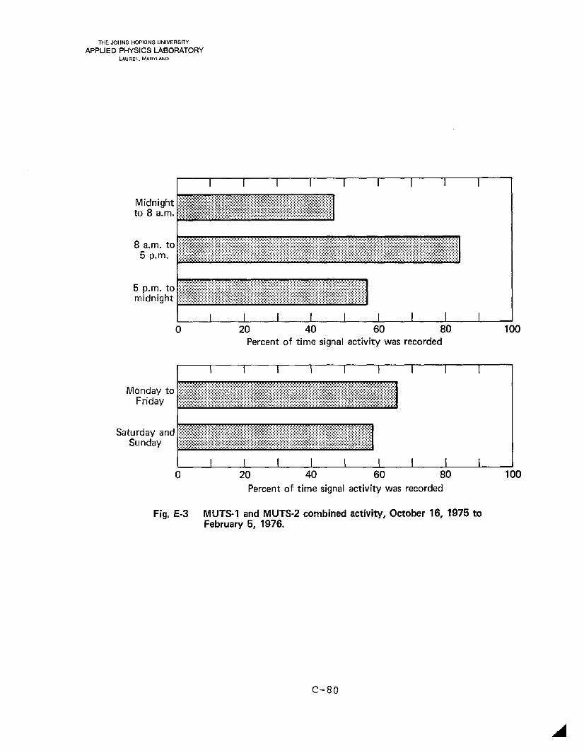
THE JOHNS HOPKINS UNIVERSITY
APPLIED PHYSICS LABORATORYLAUREL, MARYLAND
I r I I I r I I I
aI I I I I I I I
20 40 60 80Percent of time signal activity was recorded
I100
I 1 I I I T I I I
aI I
20I I
40I I
60I I
80I
100Percent of time signal activity was recorded
Fig. E-3 MUTS·l and MUTS-2 combined activity, October 16, 1975 toFebruary 5, 1976.
C-80
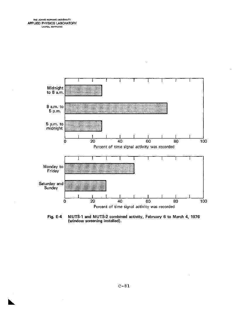
THE JOHNS HOPKINS UNIVERSITY
APPLIED PHYSICS LABORATORYLAUREL. MARYLAND
I I I I I I I I I
oI I I I I I I I
20 40 60 80Percent of time signal activity was recorded
I100
I I I I I I I I I
oI I I I I I I I
20 40 60 80Percent of time signal activity was recorded
I100
Fig. E·4 MUTS·1 and MUTS-2 combined activity, February 6 to March 4, 1976(window screening installed).
C-81


UNITED STATES DEPARTMENT OF COMMERCENational Telecommunications andInformation AdministrationWashington, D.C. 20230
APPENDIX
WORK STATEMENT
To Satisfy A Recommendation In the
Foreign Service Health Status Study
BACKGROUND
The Foreign Service Health Status Study Recommendation
The recent Foreign Service Health Status Study of JohnsHopkins University examined the possible difference in healthstatus between personnel assigned to the Moscow Embassy duringa given time period and the comparison study group. Oneenvironmental agent present in Moscow but not present at othersites was a microwave environment generated by Soviet installations.
The following recommendation is contained in the study:
There is also a need for an authoritativebiophysical analysis of the microwave fieldthat has been illuminating the Moscow Embassyduring the past 25 years with assessmentsbased on theoretical considerations of thelikelihood of any biological effects. Sufficient data was not made available to haveincluded such an analysis in the presentstudy, although much information on themicrowave field has been collected by theDepartment of State and is now available. 1/
1/ Lilienfeld, Abraham M., James Tonascia, Susan Tonascia,Charlotte H. Libauer, George M. Cauthen, Jan Alan Markowitz,and Sally Weida, Foreign Service Health Status Study:Evaluation of Health Status of Foreign Service and OtherEmployees from Selected Eastern European Posts, Departmentof Epidemiology, School of Hygiene and Public Health, TheJohns Hopkins University, Baltimore, Maryland 21205.Final Report (July 31, 1978). p. 247. NTIS Accession No.PB 288 163.
June 1979

To carry out the recommendation properly, it is desirable tohave a somewhat fuller understanding of the reason for it andits intended purpose and scope. The following discussionamplifies these points.
Reason for Recommendation
The reason for the recommendation is to specify the differencein exposure to microwave radiation, as one environmentalagent, between the Moscow study group and the comparison studygroup. This would be done by establishing the characteristicsof the microwave field at the u.s. Embassy in Moscow. Therecommendation is responsive to reviewers' comments that thenature of the microwave environmental agent was not fullyenough treated.
Purpose Intended by the Recommendation
The purpose of the recommendation is to help form an ~ prioriestimate of the likelihood of any biological effects, forcomparison with the ~ posteriori results of the hypothesesthat were tested by the epidemiological health status study.
In this connection the physical characteristics of the field as tofrequency range, spectral distribution, modulation, intensity,and duration are of interest because these physical parametersare the ones that interact with a biological system to influencethe occurrence of any biological effect. Biophysical researchresults in this area are reported in terms of the physicalparameters of exposure. Thus, in order to try to relate theMoscow exposure to the available research results, as completea physical description of the Moscow field as possible is needed.
Additionally, in order to relate any similar future studies tothe present study, the Moscow exposure field should be wellcharacterized.
OVERALL PROGRAM
The overall program would consist of three phases:
o Phase 1. The National Telecommunications and InformationAdministration (NTIA) will arrange for a determination ofthe frequency, modulation, intensity, and duration of themicrowave field in the period of interest for an adequatenumber of different locations within the Embassy duringthe period of interest.
-2-
o Phase 2. The Department of State will, on the basis ofthe Phase 1 information, provide NTIA with an estimateof greatest and typical exposures for model personnelduring this period in terms of their work and livinglocations and work programs.
o Phase 3. The Electromagnetic Radiation Management AdivsoryCouncil (ERMAC) and such other experts in biomedicaleffects of nonionizing radiation who shall act as consultantsto NTIA will provide an opinion as to whether existingknowledge of biological interactions could imply likelihoodof biomedical hazards, given the results of Phases 1 and 2.
DETAIL OF PHASE I PROGRAM PLAN
Data Base
Data on the nature of the microwave signal have been collectedfrom 1962 to the present. The data over the period 1962-1977will be the subject of the study. These consist of:
o Strip chart recordings of the average externalimpinging field averaged over time and frequency.
o Various point measurements, internal and externalto the Embassy, designed to characterize theenvironmental field more specifically and/or tocalibrate the level of the strip chart instruments.These data have been incorporated in various"highlight" reports throughout this period.
o Various special measurement programs, such asPandora, which at specific times during thisperiod have made more extensive measurementsand which have developed detailed spectral data.
o Various information about the location of thesources and the spatial extent of the beams,as available.
Data Reduction Plan
Since it is not possible to precisely ascertain the field atany given point within the Embassy at any given time, a modelwill be developed which will:
-3-

o Permit approximate calibration of strip chartvalues by means of the specific quantifiedreadings and by review and assessment of instrumentation used at the Embassy.
o Allow estimates to be made of maximum probablevalues for any given strip chart value at positionswithin the Embassy having any possibility ofexposure which may not have records of specificreadings.
o Develop the model in the time domain to permit avisual and understandable interpretation of thetime duration of the various signals involved.
Emphasis will be on trying to establish what the maximumprobable intensity is at points within the Embassy since it isexpected that the variability and lack of precise calibration,along with estimates that will have to be made of positionsof objects, reflections, attenuation of barriers, etc., cannotpermit precise determination at any given level.
Insofar as the data permit, suitable descriptions will beprovided of the spatial, temporal, spectral, and modulationcharacteristics of the field.
-4-