microwave attenuation measurements and standards · nationalbureauo1standards...
TRANSCRIPT
National Bureau o1 Standards
NBS MONOGRAPH 97 Library, E 01 Admm. Bldg
APR 1 4 1967
MICROWAVE ATTENUATION
MEASUREMENTS AND STANDARDS
U.S. DEPARTMENT OF COMMERCE
NATIONAL BUREAU OF STANDARDS

THE NATIONAL BUREAU OF STANDARDS
The National Bureau of Standards is a principal focal point in theFederal Government for assuring maximum application of the physi-
cal and engineering sciences to the advancement of technology in
industry and commerce. Its responsibilities include development andmaintenance of the national standards of measurement, and the provi-
sions of means for making measurements consistent with those stand-
ards; determination of physical constants and properties of materials;
development of methods for testing materials, mechanisms, and struc-
tures, and making such tests as may be necessary, particularly for
government agencies; cooperation in the establishment of standardpractices for incorporation in codes and specifications
;advisory service
to government agencies on scientific and technical problems; invention
and development of devices to serve special needs of the Government;assistance to industry, business, and consumers in the development andacceptance of commercial standards and simplified trade practice
recommendations; administration of programs in cooperation Avith
United States business groups and standards organizations for the
development of international standards of practice; and maintenancej
of a clearinghouse for the collection and dissemination of scientific,
technical, and engineering information. The scope of the Bureau'sactivities is suggested in the following listing of its three Institutes
and their organizational units.
Institute for Basic Standards. Applied Mathematics. Electricity.
Metrology. Mechanics. Heat. Atomic Physics. Physical Chem-istry. Laboratory Astrophysics.* Radiation Physics. Eadio Stand-ai-ds Laboratory:* Radio Standards Physics; Radio StandardsEngineering. Office of Standard Reference Data.
Institute for Materials Research. Analytical Chemistry. Poly-
mers. Metallurgy. Inorganic Materials. Reactor Radiations. Cryo-genics.* Materials Evaluation Laboratory. Office of StandardReference Materials.
Institute for Applied Technology. Building Research. Informa-tion Technology. Performance Test Development. Electronic Instru-
mentation. Textile and Apparel Technology Center. TechnicalAnalysis. Office of Weights and Measures. Office of EngineeringStandards. Office of Invention and Innovation. Office of TechnicalResources. Clearinghouse for Federal Scientific and Technical
Information.**
*Located at Boulder, Colorado 80302.
**Located at 5285 Port Royal Road, Springfield, Virginia 22151.
UNITED STATES DEPARTMENT OF COMMERCEAlexander B. Trowbridge, Acting Secretary
NATIONAL BUREAU OF STANDARDS • A. V. Astin, Director
Microwave Attenuation Measurements
and Standards
Robert W. Beatty
Institute for Basic Standards
National Bureau of Standards
Boulder Laboratories
Boulder, Colorado 80302
National Bureau of Standards Monograph 97
Issued April 3, 1967
For sale by the Superintendent of Documents, U.S. Government Printing Office
Washington, D.C. 20402 - Price 25 cents

Library of Congress Catalog Card No. 66-62097
Preface
This publication is an introductory, inclusive review of
microv\rave attenuation measurement methods and stand-
ards. It presents some relatively new material on basic
concepts including a more rigorous analysis of mismatch
and connector errors.
Particular attention is given to analysis and discussion
of errors in methods that permit the highest precision. The
means by which confidence is developed in attenuation
standards are described, and criteria are given which attenu-
ators should satisfy if they are to be worthy of precise
cahbration. Methods of measurement are classified, in-
cluding those not requiring any attenuation standard, and
each method is evaluated on the basis of convenience and
accuracy.
A list of selected references, covering most of the
significant developments in the field, is included.

ContentsPag
Preface jjj
1. Introduction 1
2. Definitions of attenuation, error analyses 22.1. Selection of a model for an attenuator 22.2. Insertion loss 3
2.3. Substitution loss 42.4. Analysis of substitution loss 62.5. Expression for insertion loss 82.6. Expression for attenuation 82.7. Analysis of attenuator calibration 92.8. Analysis of mismatch and connector errors 102.9. Intrinsic attenuation 12
3. Standards of attenuation , 143.1. Power ratio standards at d-c and audio frequencies 14
a. Power ratio standards at d-c 14b. Power ratio standards at audio frequencies 14
3.2. Broadband attenuators 153.3. Waveguide-below-cutoff attenuators 15
a. General considerations 15b. Dimensional tolerances and accuracy of measurement of displace-
ment 17c. Skin depth corrections 18d. Loading effects 18e. Mode purity 18
3.4. Rotary vane type attenuators 194. Types of attenuators suitable for calibration 20
4.1. Criteria for suitable attenuators 204.2. Coaxial attenuators 214.3. Attenuators in rectangular waveguide 21
5. Measurement methods 225.1. Classification of methods 225.2. D-c substitution 235.3. Audio substitution 255.4. IF substitution 27
a. General considerations 27b. Discussion of errors 28
Introduction 28Mismatch errors 28Converter errors 29Instability of signal source 29RE leakage 30IF leakage 31
Errors in standard attenuator 31
Noise 31Errors from connectors or waveguide joints and from waveguide or
cable 32Errors associated with the device under test 32Overall error 33
5.5. Modulated subcarrier 335.6. Direct substitution 345.7. Short-circuited attenuator 375.8. Methods not requiring attenuation standards 385.9. Measurement of small attenuation 40
6. Conclusions 41
7. References 42
iv

Microwave Attenuation Standards and
Measurements
R. W. Beatty
A comprehensive and commentarial review of microwave attenuation
measurement methods and standards is presented. In addition, a rela-
tively new and more precise way of representing and ansdyzing an attenua-
tion measurement is presented. This in turn permits more rigorous
definitions and error analyses than were previously possible. Expressions
for both mismatch and connector errors are presented.
The referral of microwave attenuation measurements to standards
operating at lower frequencies is discussed with particular attention to
the errors in the referral processes as well as the errors in the standards
themselves. Standards operating at d-c, audio frequencies, and higher
frequencies are included in this discussion which covers waveguide-below-
cutolf attenuators and rotary vane attenuators.
Desirable characteristics are Usted for attenuators which are suitable
for calibration, and examples of these are given.
Measurement methods are classified and described, giving greatest
emphasis to the intermediate-frequency substitution method using a
waveguide-below-cutoff standard attenuator, and to d-c substitution tech-
niques. Methods for measurement of small attenuations as well as methodsnot requiring reference to any standard attenuators are covered.
Comments are made on the accuracy and convenience of various
methods, and references are given which cover most of the basic and !
important research in this field.
Key words: Microwave, attenuation, measurements, standards, tutorial.
1 . Introduction
The measurement of microwave attenuation is a rather complex sub-
ject about which much has been written. There are subtle concepts
involved and unfortunately, failure to handle them carefully has resulted
in occasional disagreement and confusion. Thus it is important that
we agree, at least in these remarks, on certain definitions and termswhich will be used.
A model to represent an attenuator will be chosen from which quan-
titative definitions will be drawn. The analysis of mismatch errors andthe effects of connectors on the measurement of attenuation wiU becarefully considered. The analysis wiU initially be as general as pos-
sible, and special cases will then be considered.
Standards of attenuation will be discussed, as well as methods of
measurement which do not require reference to a standard attenuator.
The types of attenuators which are considered suitable for calibration
will be briefly mentioned, and various measurement methods will bedescribed.
The discussion of measurement methods wiU pay special attention to
sources of error and their reduction through the employment of goodexperimental practices.
In conclusion, an evaluation of the present state of the art as well as
some predictions of future developments will be attempted.
1

2. Definitions of Attenuation, Error Analyses
2.1. Selection of a Model for an Attenuator
Before defining attenuation for our purposes, it is convenient to choosea model which corresponds as closely as possible to actual situations
to be encountered. We can then base quantitative definitions and the
analysis of errors on this model.
It has been customary to use as a model for an attenuator a two-port,
as shown in figure 1(b), to which one has access by means of ideal wave-guide leads (or uniform, lossless transmission hues). Although this
has proven satisfactory for most purposes and will no doubt continue
to be used, it is not satisfactory when extremely precise results are
desired. A sUghtly more comphcated model as shown in figure 1(c)
will be initially considered. This model is a more faithful representation
of the actual situations encountered and permits more regorous defini-
tions and analyses. This approach is used because it will give a truer
picture of what actually occurs in an attenuation measurement.
COMNECTOR PAIRS ^
KERNEL OF
ATTENUATOR(a)
TERMINAL SURFACE ORREFERENCE PLANE
IDEAL WAVEGUIDELEAD
(b)
WAVEGUIDE JUNCTIONOR 2 -PORT
Dr. I Br,
TERMINAL SURFACE
PORTION WHICH- REPRESENTS -
ATTENUATOR
(C)
Figure 1. Two models to represent an attenuator.
(a) an attenuator, (b) a two-port representation, (c) use of three cascaded two-ports to represent an attenuator connected
in a system. Connector pairs are represented by two-ports A and C. The individual connectors are not separately
represented by two-ports but are designated by Dt.. &(. Bi . and Di.,
2

The simpler model which is normally used wiU be regarded as a special
case of the more rigorous model, and the assumptions required to derive
the usual equations wiU then be clearly stated.
The case of a single fixed attenuator is considered first in detail.
Consideration of variable attenuators follows in outline form.
2.2. Insertion Loss
When an attenuator is used between a generator and a load, one is
interested in its effect on the power Pl absorbed by the load. Pl is also
called the power dehvered to the load, the net power to the load, the
power received at the load, and the power dissipated in the load — all of
these terms being equivalent.
The procedure in an attenuation measurement is simply to open upthe waveguide system at some point, insert the attenuator, and note the
relative powers absorbed by the load. In the case of a variable attenu-
ator, it is inserted and remains in the circuit while it is adjusted from aninitial setting to a final setting. Again, the relative powers absorbed bythe load are noted.
Because of the insertion process, it is generally regarded that oneactually measures insertion loss or changes of insertion loss by the aboveprocedures. This is certainly true, if the definition of insertion loss [1]^
is the ratio, expressed in decibels, of the power received at the load
before insertion of the attenuator, to the power received at the load after
insertion. Note that nothing is said about the initial condition of the
system which wiU depend upon the characteristics of the connectorpair at the insertion point. This is one defect of this concept when onedesires precise terminology.
Note also that the 1953 IRE standard [1] gives two definitions for
insertion loss; a general one in which the system mismatch is not speci-
fied, and a particular one in which the system is non-reflecting. Onecannot have it both ways at once, since the insertion loss of an attenuator
will amount to a different number of decibels in each case. A way out
of this dilemma is to call the insertion loss in a non-reflecting system the
"attenuation." Actually this conforms to longstanding usage by early
workers at the M.I.T. Radiation Laboratory and elsewhere. Thesedefinitions still are defective in that they say nothing about the connector
pair at the insertion point in the system.
Although this definition appHes to most procedures used in attenuation
measurements, the term "insertion loss" has been associated with
various modifications [2] of this basic concept, and the exact meaninghas become unclear. In addition, the model used in the analysis of
insertion loss has been a simple one, and not truly representative of
the actual situation. One can apply a more rigorous model whichaccounts for the connector pair at the insertion point and make a different
analysis, obtaining a different equation for insertion loss. However,this would result in a situation in which two different equations wereobtained for the same loss concept.
The problem would be solved if agreement could be obtained on a
definition of attenuation in which the connector pair at the insertion
point and the system mismatch conditions were clearly specified [3].
' Figures in brackets indicate the literature references at the end of this Monograph.
3
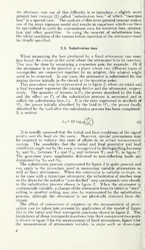
An alternate way out of this difficulty is to introduce a slightly moregeneral loss concept [2] called "substitution loss," of which "insertion
loss" is a special case. The analysis of this more general concept makesuse of the more rigorous model and results in equations which can then i
be speciahzed to yield the conventional ones for insertion loss, attenua-
tion and other quantities. In using the concept of substitution loss,
the initid condition of the system before insertion of the attenuator mustbe clearly specified.
When measuring the loss produced by a fixed attenuator, one mustfirst break the circuit at the point where the attenuator is to be inserted.
This may be done by separating a connector pair, for example. Or if
the attenuator is to be inserted at a place where two different types of
waveguides are connected together by an adapter, this adapter mightneed to be removed. In any case, the attenuator is substituted for the
joining device initially in the circuit at the insertion point.
This procedure may be represented as in figure 2, where an initial and\-_
a final two-port represent the joining device and the attenuator, respec-
tively. The quantity of interest is Pa, the power absorbed by the load,
and the effect on Pi of the substitution process is measured and is ji
called the substitution loss, Ls- It is the ratio expressed in decibels of
'Pl, the power initially absorbed by the load to ^Pl, the power finally
absorbed by the load after the substitution process has been completed.It is written
It is usually assumed that the initial and final conditions of the signal
source and the load are the same. However, special precautions maybe required to enforce this state of affairs in an actual measurementsystem. The possibility that the initial and final generator and load
conditions might not be the same is recognized by distinguishing between'be and ^ba, between ^Tq and ^Fa, and between 'Fl and ^F/, in figure 2.
The generator wave amplitudes delivered to non-reflecting loads are
designated by 'b(; and ^ba-
The substitution process represented by figure 2 is quite general andcan apply to the procedure used in measuring variable attenuators as
well as fixed attenuators. When the attenuator is variable in steps, as
is the case with a drum-type attenuator, the substitution of another step
on the drum for the initial or "zero decibel" step corresponds very closely
to the substitution process shown in figure 2. When the attenuator is
continuously variable, a change of the attenuator from its initial or "zero"setting to another setting may also be represented by the substitution
process, although the attenuator is not physically removed from the
circuit.
The effect of connectors or adapters on the measurement of atten-
uation can be taken into account by application of the model of figure
1(c) to the initial and final waveguide junctions shown in figure 2. Thebreakdown of these waveguide junctions into their component two-ports
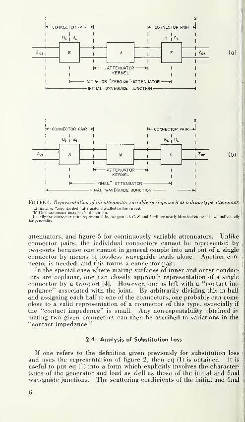
is shown in figure 3 for the measurement of fixed attenuators, figure 4 for
the measurement of attenuators variable in steps such as drum-type
2.3. Substitution Loss
(1)
4

'bo To— — Tc
SIGNAL
SOURCELOAD7 '
'-021
1 1
INITIAL WAVEGUIDE JUNCl _ .
I I
;tion -J
(a)
'bo'ro—
1
SIGNAL
SOURCEF LOAD
1 1
(b)
FINAL WAVEGUIDE JUNCTION H
Figure 2. The general representation of the situation that occurs when an attenuator
inserted into a waveguide system.
(a) In general, an adapter or a connector pair (represented by the initial waveguide junction) is initially in the wave-
guide circuit. An adapter is required to join two different kinds of waveguides which may have the characteristic im-
pedances Ziti and Zq2 as shown. When the two waveguides are alike, then ^oi=^oi> and a connector pair joins them,
(b) The attenuator and its associated connector pairs (represented by the final waveguide junction) is substituted for
the initial adapter or connector pair.
connector pair-
LloI
^01I
1^ connector pair
I
J,I
Dl
-A
-adapter kerne
ADAPTER• INITIAL WAVEGUIDE JUNCTION
(a)
CONNECTOR PAIR-
I
OoI
Bo
CONNECTOR PAIR
I
BlI
-ATTENUATOR-KERNEL
- ATTENUATOR
-
-FINAL WAVEGUIDE JUNCTION
-
(bl
(Figure 3. Representation of a fixed attenuator inserted into a waveguide system.The breakdown of initial and final waveguide junctions into their component two-port representations is shown.(a) The adapter consists of a central portion or kernel to which is attached portions of connector pairs, the connector
ion one end being in general of a different type than that on the other end.(b) The attenuator consists of a central portion or kernel to which is attached connectors which will mate with the
tconnectors belonging to the waveguide system to form the connector pairs (represented by two-ports).
229-293 O - 67 - 5
CONNECTOR PAIR-
I
Dr, 1 Jf,
• CONNECTOR PAIR-»|
I
h ATTENUATOR ^KERNEL
INITIAL OR "zero db"'ATTENUATOR
-INITIAL WAVEGUIDE JUNCTION
la)
2
H- CONNECTOR PAIR
I I I
Zo.I
AI
BI
CI
(b)
I I1*^ ATTENUATOR H I I
I I
KERNELI I
I\-> "final" ATTENUATOR H I
\» FINAL WAVEGUIDE JUNCTION H
Figure 4. Representation of an attenuator variable in steps such as a drum-type attenuator.
(a) Initial or "zero decibel"" attenuator installed in the circuit,
(b) Final attenuator installed in the circuit.
Usually the connector pairs represented by two-ports .-i, C, E, and F wiU be nearly identical but are shown individually
for generality.
I
B,
CONNECTOR PAIR
-
I
5oI
attenuators, and figure 5 for continuously variable attenuators. Unlike
connector pairs, the individual connectors cannot be represented by,
two-ports because one cannot in general couple into and out of a single ,
connector by means of lossless waveguide leads alone. Another con-,
nector is needed, and this forms a connector pair. '{
In the special case where mating surfaces of inner and outer conduc-tors are coplanar, one can closely approach representation of a single
connector by a two-port [4]. However, one is left with a "contact im-
pedance" associated with the joint. By arbitrarily dividing this in half
and assigning each half to one of the connectors, one probably can comeclose to a valid representation of a connector of this type, especially if
the "contact impedance" is small. Any non-repeatabihty obtained in
mating two given connectors can then be ascribed to variations in the
"contact impedance."
t
2.4. Analysis of Substitution Loss :
If one refers to the definition given previously for substitution loss I
and uses the representation of figure 2, then eq (1) is obtained. It is|
useful to put eq (1) into a form which explicitly involves the character- i;
istics of the generator and load as well as those of the initial and final !
waveguide junctions. The scattering coefficients of the initial and final
6
CONNECTOR PAIR- • CONNECTOR PAIR -A
»— INITIAL SETTING,—ATTENUATOR KERNEL
• ATTENUATOR
-INITIAL WAVEGUIDE JUNCTION-
CONNECTOR PAIR-
Dr. IB,
CONNECTOR PAIR -J
I
• FINAL SETTING, 1
ATTENUATOR KERNEL
ATTENUATOR
FINAL WAVEGUIDE JUNCTION
-
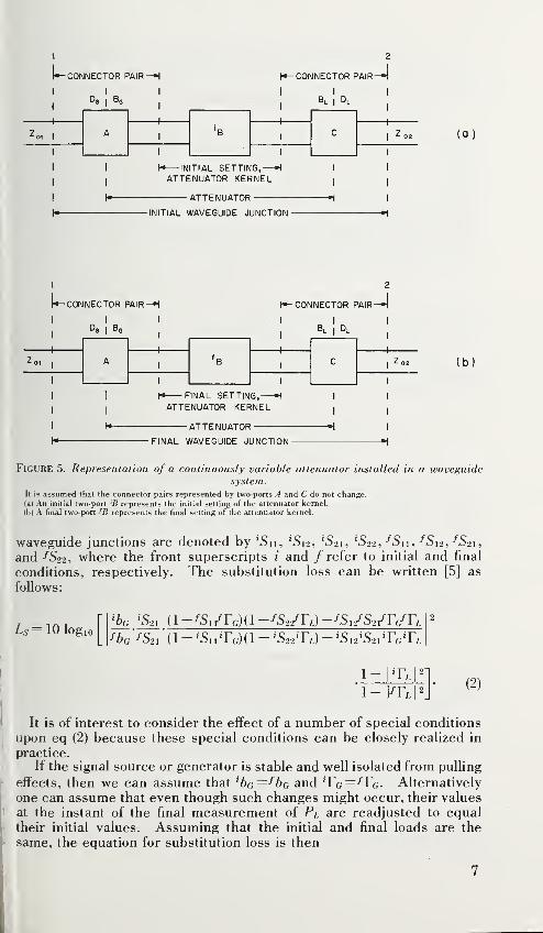
Figure 5. Representation of a continuously variable attenuator installed in a waveguidesystem.
It is assumed that the connector pairs represented by two-ports A and C do not change.
(a) An initial two-port 'fi represents the initial setting of the attenuator kernel.
(b) A final two-port represents the final setting of the attenuator kernel.
waveguide junctions are denoted by '5ii, 'S12, 'S21, '522, ^Sn, ^Si2, '^521,
and -'^522, where the front superscripts i and / refer to initial and final
conditions, respectively. The substitution loss can be written [5] as
foUows:
Ls=\0 logio%: 'S-n {i-fs^/Ya)a-fs,-/Y,)-fSv/S2/r(/r,
^ba ^S-n (l-'S„Tr;)(l-'S22Tj-'S,2*S2,'rf;*r/.
1- IT,
I
1 - VTl(2)
It is of interest to consider the effect of a number of special conditions
upon eq (2) because these special conditions can be closely realized in
practice.
If the signal source or generator is stable and well isolated from puUing
effects, then we can assume that ^ba—^bc and ^Ta=fYa. Alternatively
one can assume that even though such changes might occur, their values
at the instant of the final measurement of Pl are readjusted to equaltheir initial values. Assuming that the initial and final loads are the
same, the equation for substitution loss is then
7

Is- = 20 logio^ (1 -^SnTrOd -fS22r,)-fs,-/S2^rarL
/s.,, '(1 - 'Snr(;)(i - >s->-ii\) - 'S,2'52,r(..r/.(3)
2.5. Expression for Insertion Loss
In the definition given for insertion loss, the initial condition of the
system is not usually specified, but in many analyses [6], it is assumedthat the system can be broken apart at the insertion point without intro-
ducing any discontinuity. This is equivalent to considering insertion
loss as a special case of substitution loss, in which the initial waveguidejunction is a perfect connector or adapter (one having no dissipative
loss, no reflection, and no phase shift). For such an adapter, the scat-
tering coefficients will satisfy the following relationships:
'Si I ='S22 = 0 (non-reflection),
'Si2 = ^^'52i (reciprocity), and
'Si2'S2i = 1 (no dissipative loss and no phase shift). (4)
Substitution of these conditions into eq (3) yields the following equationfor the insertion loss:
L/ = 10 logioZo2
.^01
(1 - 5„rG)(i - S22TL) - 5,252,ro-rz.
S2A\-IgIl) (5)
The above expression gives the insertion loss of the final waveguidejunction which represents the attenuator. The representation by a
single two-port as in figure 1(b) is tacitly assumed, since it would makelittle sense to assume that the connectors were perfect in the initial wave-guide junction but not in the final waveguide junction. In the usual
case, the waveguides are practically identical and propagating a single
mode so that one conveniently sets Zo =Zo2 in eq (5).
It is observed that the insertion loss cannot be considered character-
istic of a device because it depends upon Tf, and Tl, which are properties
of the system external to the device. A quantity more nearly charac-
teristic of a device is the attenuation.
2.6. Expression for Attenuation
Attenuation is defined as the insertion loss in a nonreflecting system.
It is obtained from eq (5) by setting Fa— F/, = 0, as follows:
^ = 10 logio"Z02 1
"
Zoi'\S2l\\(6)
It is characteristic of the two-port used to represent the attenuator
and is characteristic of the attenuator to the degree that the two-port
actually represents the attenuator. The faithfulness of such a repre-
sentation depends upon the excellence of the connectors and/or adapters
of the attenuator and of the system in which it is measured.
8

2.7. Analysis of Attenuator Calibration
In the calibration of an attenuator, it is universal practice to reducethe reflections of the system to a low level before observing the substitu-
tion loss. In the limit as Fa and F/, approach zero, the substitution loss
according to eq (3) becomes
[Ls]rf; = r/ = 0= 20 logio
This is seen to be the difference between the attenuations of the final
and initial waveguide junctions.
Usually the initial waveguide junction represents a connector pair as
shown in figure 6, formed of connectors similar to these on the attenuator
under test. Although connectors are designed and constructed so as
to closely approximate ideal conditions, they will have some dissipative
loss and some loss due to reflection.
Thus the attenuation of the initial waveguide junction may be small,
but is not zero, and the measured substitution loss does not equal the
attenuation of the final waveguide junction. It should be noted that
improved connectors have been developed, and if they are used, the needfor the more precise analysis given here is diminished or even eliminated.
For various reasons, improved connectors are not yet in general use, so
that the precise analysis is needed if precise results are desired.
(7)
SIGNAL
SOURCE
CONNECTOR -HPAIR
LOAD
SIGNAL
SOURCE
• CONNECTOR -
PAIR
Dg,B
'GI°G
-ATTENUATOR
A B C LOAD
CONNECTOR-PAIR
B,I
Dl
Figure 6. Representation of usual case of insertion of an attenuator into a waveguidesystem.
9

Actually, one may not really wish to measure the attenuation of thefinal waveguide junction. Instead, it may be more desirable to knowthe substitution loss in a nonreflecting system having a standard connec-tor at the insertion point. This is a more reaHstic quantity to measureand is more characteristic of the attenuator. It is called the standardattenuation.
An expression for the standard attenuation M is obtained from eq (7),
replacing '"S21 by its equivalent expression which involves the scatteringcoefficients of the cascaded two-ports A, B, and C, and replacing 'S->\ bydn, the corresponding scattering coefficient of D- (It is understood that
the connector pair represented by D is made strictly according to stand-ard specifications.)
M=20 log.o [(1 — a>2bii){l — 622C11) — a-iibvihiCu]a-nb-nc-n
(8)
In the special case when the connector pairs are all identical and non-
reflecting (but have some dissipative loss), the standard attenuation
becomes
[M]rf; = r; =611 = ci, = 0=^.1 + ^B- (9)
This is the attenuation of the kernel B plus that of one connector pair A.
Since one portion Ba of connector pair A belongs to the attenuator andthe other portion is identical to connector Bi,, eq (9) is a quantity that is
characteristic of the attenuator itself. It follows that to the first order,
the standard attenuation given by eq (8) is also characteristic of the atten-
uator itself.
Thus the quantity actually measured in an attenuator calibration is
most closely represented by the standard attenuation. This is the sub-
stitution loss in a nonreflecting system when the initial waveguide junc-
tion is a standard connector pair. It is a quantity characteristic of the
attenuator.
The analysis of the calibration of variable attenuators follows along
the same lines and has been described in detail in the literature [7].
2.8. Analysis of Mismatch and Connector Errors
The errors in the measurement of standard attenuation due to mis-
match and to connector deficiencies have been analyzed [7]. The basis
for the analysis is shown in figure 7. The attenuator is first installed
in a nonreflecting system joined by a standard connector pair, and then
in a system having reflections and joined by a nonstandard connector
pair. The substitution loss in the first case is the desired standard
attenuation and in the second case corresponds to what is actually
measured. The difference in the substitution losses in the two cases
is the error €5. It can be resolved into three components ej, en, and
€[11, which can be written as follows:
e, = {Ao-AH) + {Ap-AA)+ {AQ-Ac),
10
(10)
€11= 20 logio
-20 logio
+ 20 logio
Cm = 20 logio
(1 — P226ii)(l ~ bj-zqn) — P2ibv2b-2iq \i
1 — P22911
(1 — a226n)(l — 622011) — a-22bvibnC\i
1 —piiqn
1 — a22Cll
and1 — a22Cii
(1 -f^SuTcMi -^^S22r/j -/^Si/^S2,rf;r,.
-20 logio
1 - rr,r,,
(1 - Aiir(;)(l - A22r0 - hr^htxYc;^ ^
1 - r^rz.
(11)
(12)
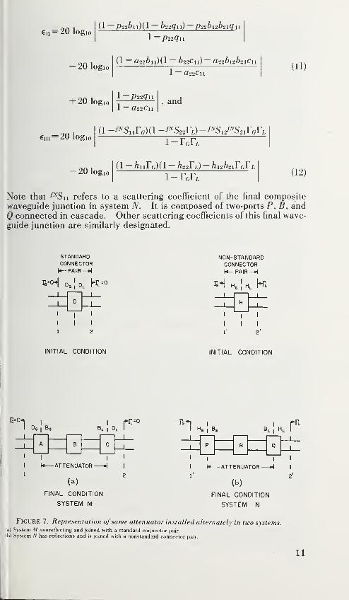
Note that -^^Sn refers to a scattering coefficient of the final compositewaveguide junction in system A'^. It is composed of two-ports P, B, and
Q connected in cascade. Other scattering coefficients of this final wave-guide junction are similarly designated.
STANDARDCONNECTORh— PAIR—
H
d,|d, K=o
I
I
I
I I I
1 2
INITIAL CONDITION
NON-STANDARDCONNECTORh- PAIR—
H
1
H
1
1 1
I I
INITIAL CONDITION
E--0
1 0,GI°G
I r;
3uI
D, I
rL=o
A B C
1
11
«• ATTENUATOR •
(a)
FINAL CONDITION
SYSTEM M
eI
"0 3lI
H, I
1
p B Q
1
1 1
• ATTENUATOR M I
2'
(b)
FINAL CONDITION
SYSTEM N
Figure 7. Representation ofsame attenuator installed alternately in tuio systems.(a) System M nonreflecting and joined with a standard connector pair.
(b) System /V has reflections and is joined with a nonstandard connector pair.
11
The error component ej consists of differences of attenuations of con-
nector pairs and will vanish if corresponding connectors Da = Ha andDi^ = Hl, since it then follows that D = H, A = P, and C = Q. This is
a sufficient but not necessary condition, since €] will vanish also whenAd + Ap+ Aq = Ah+Aa+ Ac- Usually the corresponding connectorpairs D and H will be similar, so that ej may be less than 0.01 decibel
(dB). Evidently, it is desirable to make D and H identical, or in other
words to use standard connectors at the insertion point.
The error component Cn consists of terms similar to eq (5). It is the
difference between the insertion losses of the attenuator kernel B if
installed alternately into two nonreflecting systems in which the con-
nector pairs A, C, P, and Q had reflections. This is a hypothetical
situation, and one in which identity of the corresponding connectors
Da = Ha, and Dl = Hi, would also cause en as well as €] to vanish. Sinceordinarily the connector pairs at the insertion point are quite close to
standard connectors, this error component will normally be small (of
the order of 0.001 dB or less).
The error component em differs from the other components in that
it does not necessarily vanish if Da = Ha and Dl = Hl. However, it
wiU vanish if the system reflection coefficients Ta and vanish.
It is the most significant of the error components and may well exceed0.01 dB if the VSWR of the system exceeds 1.02. The vanishing of
Fa and Ti, is a sufficient but not a necessary condition for the vanishingof em. This is apparent since the two terms may cancel due to for-
tuitous amplitude and phase relationships of the scattering and reflection
coefficients involved.
The above analysis reduces to the usual analysis [6, 7, 8] for mis-
match error using a simpler model, if we assume that the connectorsare all nonreflecting, lossless, and introduce no phase shift. In this
case ej and Cn vanish, and em reduces to [7].
€m = 20 logio(1 - 6„r(;)(l - b2>rL) - br-zb-nVar,.
i-r^r. (13)
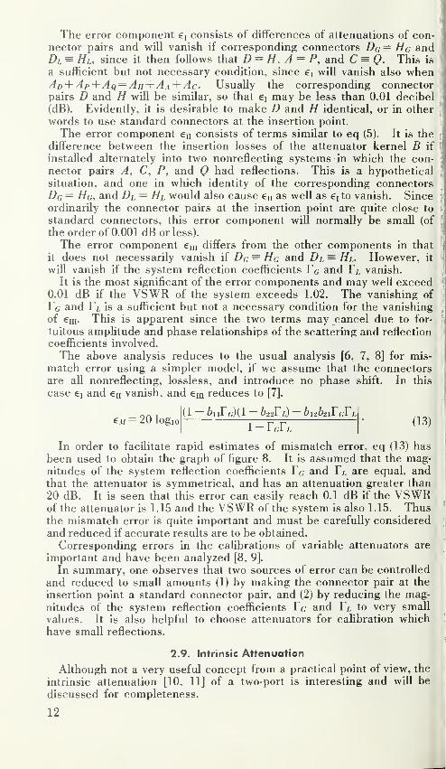
In order to facilitate rapid estimates of mismatch error, eq (13) has
been used to obtain the graph of figure 8. It is assumed that the mag-nitudes of the system reflection coefficients Va and Yi. are equal, andthat the attenuator is symmetrical, and has an attenuation greater than
20 dB. It is seen that this error can easily reach 0.1 dB if the VSWRof the attenuator is 1.15 and the VSWR of the system is also 1.15. Thusthe mismatch error is quite important and must be carefully considered
and reduced if accurate results are to be obtained.
Corresponding errors in the calibrations of variable attenuators are
important and have been analyzed [8, 9].
In summary, one observes that two sources of error can be controlled
and reduced to small amounts (1) by making the connector pair at the
insertion point a standard connector pair, and (2) by reducing the mag-
nitudes of the system reflection coefficients Ta and to very small
values. It is also helpful to choose attenuators for calibration whichhave small reflections.
2.9. Intrinsic Attenuation
Although not a very useful concept from a practical point of view, the
intrinsic attenuation [10, 11] of a two-port is interesting and will be
discussed for completeness.
12

1.001 1.002 I.OI 1.02 I.IO 1.20
VSWR OF SYSTEM
Figure 8. Graph for rapid estimates of limits of mismatch error.
The intrinsic attenuation can be defined as the attenuation of three
two-ports in cascade: the inner two-port represents the attenuator andthe other two represent lossless tuners that have been adjusted to elim-
inate reflections Sii = Sz2= 0 for the composite two-port). The fact
that it is always possible to make such an adjustment is seen by con-
sidering what has been called [12] the "modified Wheeler network."The intrinsic attenuation is never greater than, and usually less than,
the attenuation of the two-port representing the attenuator. Hence,it should be possible to reduce the attenuation by the use of tuners as
described above. However, in a practical situation, it may be foundthat the losses added due to dissipation in the tuners may exceed the
expected reduction in attenuation.
Another way of defining the intrinsic attenuation of a two-port makesuse of its efficiency 7], the ratio of net power output to net power input.
The efficiency depends upon the reflection coefficient Yl of the load andwill be maximum rjM for a particular value Ym of F/,.
The intrinsic attenuation Ai is then given by
.4/= 10 logio— , (14)J?.v/ ^ '
229-293 O - 67 - 313

where
(15)
and
(16)
where ^ =5^2 + 5* (SiaS,, -SnSaa), and 5 = 1 - iSn P + - |S,252,
-SnS.,2|2.
It is evident that for a reciprocal two-port the intrinsic attenuation is
the same regardless of the direction of energy flow through the two-port.However, for a nonreciprocal two-port, there will be two different in-
trinsic attenuations, one for each direction of energy flow.
3. Standards of Attenuation
3.1. Power Ratio Standards at D-C and Audio Frequencies
Power ratio standards developed at d-c and audio frequencies are not
only important at these frequencies but are useful at much higher fre-
quencies where substitution devices and techniques have been devel-
oped. Devices such as barretter detectors accurately foUow a square-
law response over a useful range and permit one to measure ratios of
microwave signal levels by referring to audio frequency or to d-c ratio
standards.
Although attenuators or resistive voltage dividers [13] which operate
at d-c are commercially available, they are not as widely used as poten-
tiometers. The potentiometer has been highly developed and is a
versatile instrument that is available in most laboratories.
In order to determine d-c power with a potentiometer, one ordinarily
measures the current through a resistor of known value. The uncer-
tainty in making such a power measurement is ordinarily small. Forexample, the current may be obtained by measuring the voltage across
a standard resistor of one ohm (known to 0.001 percent). If a voltage
of 9.0 mV is measured with a potentiometer, the uncertainty may be
0.01 percent. Consequently, the uncertainty in the measurement of a
current of 9 mA is 0.011 percent. The corresponding uncertainty in
determining the d-c power (16.2 mV) dissipated in a 200-ohm resistor,
known to an uncertainty of 0.01 percent, is 0.032 percent. The uncer-
tainty in determining d-c power ratios would then be 0.064 percent or
Somewhat lower uncertainties [13] may be obtained with commerciallyavailable equipment of higher quality. An order of magnitude improve-
ment is possible (0.0064 percent, or 0.00028 dB in power ratio).
Inductive voltage dividers or ratio transformers have been developedas standards of voltage ratio at audio frequencies. Commercially avail-
able units may have a typical ratio uncertainty of 0.001 percent + 0.0006percent ratio. Variations of the uncertainty calculated from this
a. Power Ratio Standards at D-C
0.0028 dB.
b. Power Ratio Standards at Audio Frequencies
14

formula are shown in table 1. For ratios near unity or below 1 dB, the
uncertainty remains at 0.0016 percent or 0.00014 dB. At lower ratios,
the uncertainty continues to rise, reaching 0.6 percent or 0.052 dB for
a ratio of 0.001 or 60 dB.
The inductive voltage divider is usu^Uy quite stable and can be cali-
brated [14] in order to obtain somewhat greater accuracy. Perhaps an
order of magnitude decrease in the uncertainties in voltage ratios
quoted in table 1 is possible. Cahbration of these inductive voltage
dividers may be carried out with respect to capacitance standards,
[15] or by other methods [16] which have been recently developed.
The frequency range of most commercially available inductive volt-
age dividers is 30 to 1,000 Hz, and some wiU operate at 20 kHz.
Table 1. Typical uncertainty in the ratio of a commer-cially available inductive voltage divider
Ratio Ratio in
decibels
Uncertainty
Percent Decibels
0.900 0.9152 0.00166 0.00014
.500 6.0206 .0022 .00019
.100 20.000 .0070 .00061
.010 40.000 .061 .0053
.001 60.000 .601 .052
3.2. Broadband Attenuators
At frequencies above approximately 1 kHz, most inductive voltagedividers become less accurate due to capacitance effects, and broad-band drum-type attenuators are used as standards. Carbon-film,TT-section attenuators having 0.1-dB steps have been made [17] thatdo not exhibit much change in attenuation from d-c to 1,000 MHz. l- orfrequency changes from 0 to 200 MHz, corresponding changes in at-
tenuation were less than 0.1 dB and up to 1 GHz were less than 1 dB.In addition, metallic film attenuators are commercially available
which operate from d-c to microwave frequencies. Some of these arequite stable and are available in drum-type attenuators having 0.1-dBsteps and a range of 0 to 64 dB. They have a frequency range from d-cthrough 2 GHz and an uncertainty, when cahbrated, of 0.02 dB per 10dB, or 0.02 dB, whichever is greater. It is possible to obtain speciallyselected single attenuators of this type which operate up to 12.4 GHzand caUbrate them to higher accuracy; but at frequencies of approxi-mately 10 MHz to 1 GHz, higher accuracy can be obtained with wave-guide-below-cutoff attenuators.
3.3. Waveguide-Below-Cutoff Attenuators
a. General Considerations [18]
A waveguide section, excited in one mode by a sinusoidal signal at
a frequency below cutoff, has an exponential decay of field strength
along its axis. The rate of decay may be closely predicted from a
knowledge of the cross-sectional dimensions of the waveguide. Amoving probe which couples to the field will therefore have a predict-
able output variation. The entire arrangement constitutes a standardof attenuation.
Practical waveguide-below-cutoff attenuators are usually made frommetal tubes of circular cross section and operated in the TEi^ i mode.
15
(Rectangular cross section is also used and has the advantages that,
there is greater separation between the cutoff frequencies of higher I
modes and the attenuation rates are relatively greater for the unwanted '
modes.)
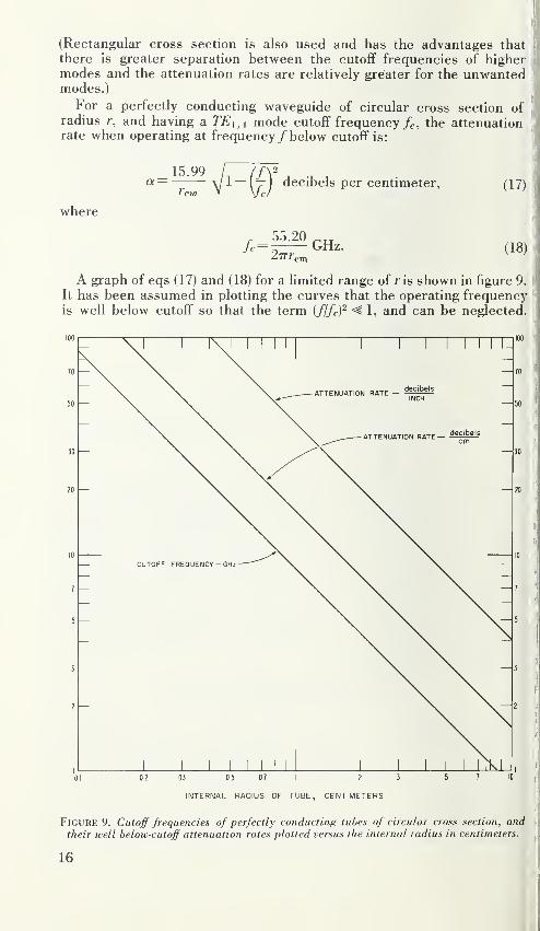
For a perfectly conducting waveguide of circular cross section ofradius r, and having a TEi,i mode cutoff frequency /c, the attenuationrate when operating at frequency /below cutoff is:
_ 15.99 r JfY ^ ^oc—
V \T I decibels per centimeter,cm ' Vc/
!
Inhere
fc55.20
27rr^mGHz.
(17)
(18) (
A graph of eqs (17) and (18) for a limited range of ris shown in figure 9. I
It has been assumed in plotting the curves that the operating frequencyis well below cutoff so that the term {fIfcY 1, and can be neglected.
CUTOFF FREQUENCY - GHz
J \ I I I I I
03 0 5 0,7 I 2 3
INTERNAL RADIUS OF TUBE, CENTIMETERS
Figure 9. Cutoff frequencies of perfrctly conducting tubes of circular cross section, andtheir well below-cutoff attenuation rates plotted versus the internal radius in centimeters.
16

It is advantageous to operate well below cutoff to reduce errors in the
attenuation rate due to any possible uncertainty in the frequency.
As one goes to higher frequencies, it is necessary to use tubes of
smaller radii in order to stay below the cutoff frequency, as seen fromeq (18). It is seen that this will result in an increased attenuation rate
according to eq (17). For a given tolerance in the radius, and for a
given uncertainty in measuring the displacement of the pickup coil,
the errors will increase. For this reason, the waveguide-below-cutoff
attenuator has not been used as a precise standard of attenuation muchI
above 1 GHz, although it has been used for direct reading variable at-
tenuators up to 11 GHz, in applications where an accuracy of ±2 dB is
I
considered satisfactory.
i As one goes to lower frequencies, the skin depth becomes appreciable
compared to the wall thickness, and waveguide-below-cutoff attenuatorsi are seldom used below 1 MHz. The skin depth in brass at 1 MHz is
iapproximately 0.005 in. The wall thickness should be much greater
!than the skin depth if leakage through the tube [18n] is to be neghgible.
jA desirable characteristic of waveguide-below-cutoff attenuators is
that the phase shift does not change as one varies the attenuation overthe linear range.
I
When used as a variable attenuator, the below-cutoff attenuator has
!the disadvantages of almost purely reactive input and output impedancesand a high residual attenuation of 20 to 30 dB. The large residual is
;due to the fact that the attenuation rate is not accurately predictable
when the separation of the pickup and exciting coils is too small. Thisminimum spacing is dependent upon both loading effects and the pres-
' ence of higher modes (to be discussed).
b. Dimensional Tolerances and Accuracy of Measurement of Displacement
1 The dimensional tolerances on the internal radius of the tube are' important. For example, a tube having a nominal radius of 0.80 cm
I
has an attenuation rate well below cutoff of approximately 20 dB per
j
centimeter. In order to keep the uncertainty in the attenuation rate to
1within 0.002 dB per centimeter, the radius must be held to the nominal
j
value to within 0.000080 cm, or 0.000032 in. Thus, close tolerances
j|imust be held in the fabrication of the tube, and electroforming techniques
Iare often used. In addition, machining and honing of stainless steel
s cyUnders have been carried out [18n].
I
At higher frequencies of operation, this problem becomes moreI critical. At an operating frequency of 30 MHz, a tube radius of 2.9
I
cm might be used, with an attenuation rate of 5.5 dB per centimeter.
Assuming an uncertainty of 0.001 cm in the radius, the correspondinguncertainty in the attenuation rate would be 0.0019 dB per centimeter.
This would result in an uncertainty of ±0.019 dB in a measurement of
55 dB.
The same 0.001 cm uncertainty in a radius of 2.9 mm, for a tube oper-I ating at 3 GHz would cause an uncertainty of 0.019 dB per centimeter;in the attenuation rate of 55 dB per centimeter. This would increase
I
the uncertainty of a 55 dB measurement to ± 1.9 dB.
IThe uncertainty in the messurement of the displacement of the pickup
' coil is also important. For example, if the attenuation rate is 5.5 dBper centimeter as in the case above, an error of 0.001 cm will cause a
17

corresponding error of 0.0055 dB at 30 MHz. At 3 GHz, with an at-
tenuation rate of 55 dB per centimeter, the same 0.001 cm error in the
measurement of displacement will cause an error of 0.055 dB.
It is clear that the dimensional tolerances on tube radius eventuallylimit the upper frequency at which below-cutoff attenuators are useful
as standards.
c. Skin Depth Corrections
The effect of the penetration of the current into the metal walls of
a waveguide is to decrease the attenuation rate by a small but appreciableamount. In a copper waveguide of circular cross section operating at
30 MHz, the skin depth is approximately 0.0005 in., and the effective
radius is increased by half [18e] this amount. Thus for a tube radius of
1.6 in. the attenuation rate might be 0.00156 dB per inch lower than that
predicted without accounting for the skin depth. One ordinarily corrects
for this in the design of the attenuator so that only the error in deter-
mining the skin depth contributes to the uncertainty in the attenuation
rate.
A nomogram [18i] is available for determining the attenuation rate of
a waveguide-below-cutoff attenuator operating in the TEj^i mode, andtaking into account the skin depth. Corresponding charts for rectangu-lar waveguide are not available, but the effect of skin depth on the propa-gation constant of the dominant mode has been analyzed [18j].
d. Loading Effects
As the coupling coils are brought closer together, there is an effect on
the input power due to loading of the input circuit by the circuit con-
nected to the pickup coil. If adequate coil separation is maintained,
this effect is negligible, but one pays a price of tolerating perhaps 30dB of initial attenuation. This limits the range over which attenuation
measurements can be made with the IF substitution technique.
Several approaches have been made to reduc^e the initial attenuation
or its effect in limiting the range of accurate measurement. Two dif-
ferent analyses [IBh], giving different results, are available to determine
the effects of loading. These effects are avoided by using a feedback
system to provide constant current to the exciting coil [18k]. Anotherapproach is to employ a separate source of energy at the intermediate fre-
quency to excite tTie below-cutoff attenuator, and to switch between the
attenuator output and the output of the mixer in the IF substitution sys-
tem [18c]. This removes the below-cutoff attenuator from the circuit
between mixer and detector and effectively increases the range of the
measurement by the amount of the initial attenuation of the below-cutoff
attenuator.
e. Mode Purity
In exciting the waveguide-below-cutoff attenuator, one attempts to
excite only the desired mode, but unless unduly elaborate exciting ar-
rangements are used, other modes will also be excited. The higher
modes will have somewhat higher attenuation rates than the desired
mode. Thus for large probe separations, the higher modes will have
18
decayed faster than the desired mode and will have negligible effect onthe output. One does not usually rely on this effect to obtain modepurity, but instead uses mode filters [18e] to attenuate the higher modes.The thickness of the mode filter then limits the closeness of separation
of the exciting and pickup coils, and this in turn limits the minimum or
residual attenuation of the below-cutoff attenuation standard.
The possibility of rotation of the polarization of the desired modeshould be reduced by careful fabrication of the tube to avoid any eccen-
tricty. This can easily be checked experimentally for a given tube.
3.4. Rotary Vane Type Attenuators [19]
The type of variable attenuator in which a dissipative resistive vane
is rotated in a section of waveguide of circular cross section has one of
the properties essential for a standard attenuator. That is, the incre-
mental attenuation can be accurately determined by calculation fromthe angle that the vane makes with the polarization of the TE^^i modein the waveguide.
In addition to its possible use as a standard attenuator, this type has
found wide use as a direct reading variable attenuator.
The attenuation is given [19d] by the expression
A = (40 logio sec d+ C)dB, (19)
where 6 is the angle of the central vane with respect to the normal to
the plane of polarization of the electric field in the TEi, i mode, and C is
a constant representing the residual attenuation when 6= 0. Tablesbased upon eq (19) are available [19h] to determine the variable com-ponent of attenuation as a function of the vane angle 6.
Errors in the incremental attenuation as given by the dial readingare usually small but are appreciable and are caused by a number of
factors, such as mismatch, drive gear imperfections, misahgnment of
end vanes, initial misahgnment of central vane, insufficient attenuation
of central vane, mode impurity in central section, perturbation of TEi, i
fields by the vane, imperfections in the rotating chokes, parallax in the
readout device, mechanical flexure of the end vanes during connectionof the attenuator in the circuit, warping of the vane, etc.
Practically aU of these errors have been investigated except for somealignment problems and perturbation of the field by the central vane.
The results [20] shown in table 2, if they can be considered typical,
cire a tribute both to the original concept upon which the attenuator is
based, and the design and construction of commercially available at-
tenuators. At present, the rotary vane attenuator is available in manysizes of waveguide operating from 2.6 to 220 GHz.At frequencies from 2.6 to perhaps 170 GHz, the waveguide-below-
cutoflf attenuator operating at 30 GHz (or 20 to 60 GHz) in an IF substi-
tution system wiU probably continue to be used to calibrate rotary vaneattenuators. Somewhat greater resolution and accuracy are available
[20] with reference to d-c standards, but the method is presently not asconvenient as the IF substitution technique. The modulated subcar-rier technique appears promising as a competitor, but comparable confi-
dence has not yet been developed.
19
f

Table 2. Results of three sets of measure-
ments on a rotary vane attenuator
Attenuator dialA fAverage oi
reading measured values
Decibels Decibels
0 0107.0214
.0303
.0407
.05 !0521
.uo 0609
.u/ 0700
,uo .0802no 0909
.1 !l021
.LZ 1 101
1 /I.14' 1 ^7"^
.10 .10 io1 o.lo . 1 /oo
.2 .2007
.250/171
.5/107Q
1
3 2.998
r0 /I Qon4-.W'J
1 AlU15 14.99
2025 25.01
30 30.07
40 40.33
50 52.24
4. Types of Attenuators Suitable for Calibration
4.1. Criteria for Suitable Attenuators
Not all types of attenuators are suitable for calibration for various
reasons. They should meet the following criteria:
1. Electrical characteristics should be stable over long periods of time(several years).
2. They should be mechanically stable and rugged so as not to undergoany permanent changes of characteristics under careful handling andshipping.
3. Changes of electrical characteristics with changes of environmental
conditions such as temperature, pressure, humidity, etc., should be
small (less than 0.01 dB over ranges encountered in various laboratories).
4. Changes of electrical characteristics with power level should besmall (less than 0.01 dB over ranges used).
5. Reflections should be small (VSWR certainly less than 1.5, prefer-
ably less than 1.15).
6. Leakage should be negligible.
20
4.2. Coaxial Attenuators
Sections of lossy cable such as RG-21/U have been used as attenua-
tion standards. These are especially attractive when average powersof 10 watts or higher are encountered. However, unless special pre-
cautions [21] are taken to eliminate flexure of the cable, especially nearthe connectors, they are not ordinarily suitable for precise work.Both T and tt configurations are used to construct attenuators in coaxial
line. The elements are rods and discs with a resistive film of graphite
or metal baked on an insulating base, then covered with a protective
insulating film. Such attenuators have been highly developed to havestable characteristics and low reflections over frequency ranges fromd-c to 12 GHz.
Coaxial attenuators having only resistive center conductors may also
be suitable for calibration over a limited bandwidth, for example 2 to
18 GHz.Extremely broadband coaxial attenuators have recently been built
using a resistive card [22] as the lossy element, and attaching leads to
certain points on the card. They are useful at frequencies from 0 to
at least 18 GHz.The use of in-hne directional coupler types of standard attenuators is
an anticipated development which should result in standard coaxial
attenuators having superior characteristics.
Ordinarily, coaxial pads can be easily checked at d-c to see whetherthere is any defect which would make them unsuitable for calibration at
higher frequencies.
Coaxial variable attenuators have been constructed using stripline androtating discs of resistive material, hybrid or ring circuits in stripline
with shding contacts, and sliding contacts on resistive cards. A capaci-
tively coupled metal slider, shorting out portions of a resistive center
conductor has been used. Variable directional coupler types of coaxial
attenuators have been very successful. In addition, flap-type variable
attenuators have been built in coaxial hne. The waveguide-below-cutoffattenuator has also been used as a basis for a variable coaxial attenuator.
Very few of these designs have met the criteria for a good standardvariable attenuator, so that more development needs to be done in this
area.
4.3. Attenuators in Rectangular Waveguide
Both fixed and variable attenuators are available in rectangular wave-guide which are suitable for calibration.
The type of fixed pad having best characteristics for a standard is the
in-line directional coupler [23] and related types. True in-line arrange-
ments can be calibrated more accurately than off^set "in-line" arrange-
ments. Fixed pads have the disadvantage that they must be inserted
and removed from the circuit during the calibration.
Single-step attenuators are available in which the in-line directional
coupler principle is used. A movable resistive vane is positioned in the
main waveguide between the two sets of coupling holes of an in-line
directional coupler. When the vane is flat against the wall of the wave-guide, energy passes through the main waveguide with very little loss.
When the vane is moved out into the electric field, it attenuates effec-
tively all of the energy which tends to pass through the main waveguide.
229-293 O - 67 - 421

In this case only the energy which passes through the coupling holesinto the auxiliary waveguide and back again arrives at the output. Thustwo steps are provided; an initial step having very little attenuation anda final step having an attenuation determined by the sets of couplingholes. Such an attenuator has a low VSWR, is not frequency sensitive
and does not need to be removed from the circuit during calibration.
However, the minimum loss position may show a small variation (less
than 0.1 dB) if the vane does not lay flat agaisnt the wall each time it
is so positioned.
Continuously variable attenuators of mainly two designs are suitable
for cahbration. These are (1) the rotary vane type, and (2) the type in
which a resistive vane moves in and out of the waveguide field, remainingparallel to the side wall.
The rotary vane type has superior resolution at the lower attenuationvalues while some models of the parallel translating vane type havehigher resolution at the higher attenuation values. The rotary vanetype has much lower phase change (less than 1 degree over the entire
range) and is less frequency sensitive than the other type.
Presently realizable accuracy [20] of attenuator calibration exceedsthe resolution to which these "precision" attenuators can be set andread; therefore, further developments are indicated.
5. Measurement Methods
5.1. Classification of Methods
A large variety of methods is available for attenuation measurements.They can be classified as follows, according to the kind of standard used:
1. D-c substitution
2. Audio substitution
3. IF substitution
4. Direct substitution
a. Series
b. Parallel
5. Methods requiring no standard of attenuation
6. OthersMany variations on, and mixtures of methods are possible, so that
the above classification scheme is not perfect. However, most of the
"standard" methods will be accommodated.Perhaps the greatest range (150 dB) has been obtained [18k] with the
i,
direct (parallel) substitution method at 30 MHz. Ordinarily up to 70dB range is obtained using the IF substitution technique, and this may
,
be extended at least 30 dB by use of a separate IF source [24] andj
switching arrangement and by combining this with direct substitution. ,
The greatest accuracy has been obtained using a d-c substitution[,
technique. Although comparable precision was obtained with a modu-lated sub-carrier method, the error evaluation of this method is not so
;
complete.j
Audio modulation methods are convenient to use with equipment^
ordinarily available in most laboratories, but have limited range and!
accuracy. However, continued refinement of the equipment, and use '
of dual channel systems, synchronous detection, and noise suppressors,5
can markedly increase the accuracy and ranges of these methods.
22

Methods requiring no attenuation standard are attractive from one
point of view — minimum equipment — but are comparatively tedious in
operation and limited in range. However, they may be quite useful
when an attenuation standard is not available.
5.2. D-C Substitution
In d-c substitution methods, some sort of converter is ordinarily usedto produce a change in d-c power bearing a known relationship to the
change in a-c power to be measured. The converter may be a crystal
rectifier, thermocouple, bolometer, etc. The "law" of the converter
must be known in order to convert from the measured d-c ratios to the
desired a-c ratio. A crystal rectifier may operate in a square-law region
at low signal levels, and in a linear region at high signal levels. Atintermediate levels, the "law" is somewhere between the two.
It is clear that a precise knowledge of how much the converter deviates
from its ideal "law" is necessary if accurate results are to be obtained.
A d-c substitution technique using bolometers (barretters or thermis-
tors) in a balanced bridge arrangement has been described [20]. In
this method, microwave power dissipated in a barretter causes a changei in its d-c resistance away from its initial value corresponding to a certain
d-c bias power. The barretter resistance is returned to its initial value
by withdrawing some of the d-c bias power. The amount of d-c powerwithdrawn is nearly equal to the microwave power dissipated in the
barretter. The ratio of the two powers is nearly unity. In order to
measure the absolute microwave power by this method, one would needto know this ratio; but in an attenuation measurement, we need to deter-
mine only the relative power. Hence we do not need to know the ratio,
but we do need to know that it is constant for a given bolometer andindependent of power level over the range of observation.
The constancy of the ratio is difficult to determine absolutely, but has
j
been investigated [25] by an experiment in which microwave power wasI fed through a power divider (3 dB directional coupler) to a barretter
j
mount and a thermistor mount. The microwave power level was varied
!
in steps over a 20 dB range, and the ratio of the d-c substituted powers
j
in the two bolometers was noted at each step. Within the experimental' error (0.1 percent) no change in the ratio was observable, indicating
either that no change occurred, or that it was identical for the two ele-
ments. However, the barretter and thermistor are sufficiently different
I
that it seems more likely that no appreciable change in the ratio occurred,
j
Since the experimental error of 0.1 percent corresponds to 0.0043 dB,f over a 20 dB range, it is reasonable to place at least this much confi-
1dence in the results of a 20 dB attenuation measurement using this d-c
I substitution technique. The confidence limit should be correspondinglyI better for attenuation smaller than 20 dB.
: Actually an error of 0.1 percent+ 0.1 /u,W in measuring power dififer-
iences can lead to errors of 0.0001 to 0.0043 dB in attenuation as theattenuation varies from approximately 0.06 to 3 dB. This follows if onemeasures directly the change in d-c power, W>—Wi, corresponding to
^
a change in the microwave attenuator rather than measuring each timei the departure from the initial bias power Wo- The error evaluation
jj
procedure is illustrated in the following example:

The attenuation A is given by
^ = 10 \og,, ^^_^ - (20)
Instead of measuring Wo~Wx and Wq—W-,, it is preferable for atten-uations less than 3 dB to measure W-y—Wu a smaller difference. Thisquantity appears exphcitly by rewriting eq (20)
An example will show the difference in the error in A as determinedby the two methods. The character of the error in measuring differ-
ences in d-c power is such that it is partially random and partially
systematic. In a particular example, it is assumed that this error hasequal random and systematic components. Thus if Wo — W\ is 0.1
percent high, Wq—W-z will be between 0 and 0.1 percent high. Let
15.00 mW, ri = 10.10 mW, and W2= 10.64 mW, so that; /4 = 0.5071
dB. If we measure Wq— Wi with an error of 0.1 percent high, obtain-
ing 4.095 mW, then the measured value of Wq—W-z wiU be between4.3600 and 4.3644 mW. We can then obtain A as high as 0.5115 dB,
or an error limit of 0.0044 dB.
Now suppose that we measure W> — W\ with an error of 0.1 percenthigh, obtaining 0.5405 mW, then the measured value of Wq—Wi will
be between 4.900 mW and 4.905 mW. We then can obtain A as high
as 0.5076 dB, or an error limit of 0.0005 dB. Thus the error hmit is
reduced to approximately one ninth of the error hmit which occurs whenmeasuring Wo — W\ and Wq — W-y.
For attenuations above 3 dB, one measures the d-c power differences
Wo-Wt and W^-W,, and uses eq (20).
In using thid d-c substitution method, it is recognized that other
sources of error wiU be present, and they must have correspondingly
low limits if one is to take full advantage of the high accuracies of d-c
standards. One must pay close attention to the reduction of systemreflections and carefully evaluate the mismatch errors. It has beenfound worthwhile to use this technique to calibrate rotary vane atten-
uators because they have quite small variations of phase shift as the
attenuation is changed, have low reflections, and have high resolution
over the lower part of their range.
Strictly speaking, any method in which the attenuation at somedesired higher frequency is obtained by reference to d-c standards canbe regarded as a d-c substitution technique. Thus the measurementof the power to a load before and after insertion of variation of the
attenuator can be a d-c substitution technique provided that the poweris measured by a method using d-c standards. The direct substitution
of d-c attenuation for the attenuation to be measured at a higher fre-
quency has not been so sidely employed because other techniques
have been easier to apply and have wider direct ranges.
24
5.3. Audio Substitution
Accurate standards of attenuation, such as drum-type attenuators
having step intervals as small as 0.01 dB, have been available for use
at audio frequencies for many years. Such standards are relatively
inexpensive and are available in most measurement laboratories. In
addition, accurately square-law converters such as barretters have also
been available and inexpensive for many years. Consequently, audio
substitution techniques of attenuation have been popular [26] in spite
of the limited range (below approximately 40 dB, directly) of the con-
verters.
Basically the method involves the following steps: modulation of the
signal source or its output, square-law detection, attenuation of the
audio frequency by a cahbrated audio attenuator, amplification, and,
finally, detection and indication.
In this substitution method, as well as aU others, a basic question
must be answered. That is, how much does the converter or detector
deviate from the assumed law? Studies have been made [27] of bar-
retters and crystal detectors, with the result that the range of use de-
pends upon the tolerable deviation from square law. If 0.2 dB is
tolerable, the crystal video diode can have a range of approximately 38dB, and the barretter a range of 53 dB. However, if less than 0.01 dBis tolerable, use of a crystal is not recommended, but a barretter has arange of approximately 20 or 30 dB.Other types of square-law detectors, such as thermistors, [28], thermo-
couples, bolomistors [29], ferrite [30] and ferroelectric [31] detectors,
and thermoelectric films [32], have also been used.
The deviations from square-law behavior are somewhat different for
each of these types of detectors. No exhaustive comparative studyhas been made; therefore, it is good practice to check the deviations
from square law when using audio substitution techniques.
One can determine this experimentally in a given system by starting
at a fairly low power level and measuring a given change of attenuation,
e.g., 1 dB, at progressively higher power levels to the detector. Whenthe observed attenuation increment changes by an amount equal to
the tolerable deviation, the power to the detector is noted. If one stays
below this power level, then deviations from square law will remainbelow the tolerable deviation. This is true because the small signal
theory of crystal and barretter detectors predicts square-law behavior,
and the smaller the signal, the closer one comes to ideal behavior.
The lower end of the range is limited by noise which increases ap-
proximately as 1//, where / is the frequency. One cannot decreasenoise indefinitely by increasing /, especially with barretters, becausetheir time constant wiU reduce their detection efficiency. Also, the
frequency ranges of audio standards such as resistive attenuators andinductive voltage dividers are hmited. Considerable reduction in the
effect of noise has been achieved by using synchronous detectionwhich effectively decreases the bandwidth.The effects of noise on errors in attenuation measurements have
been investigated [33] for different kinds of detectors. The results
apply to IF substitution methods employing audio modulation as well
as to audio substitution methods. Graphs are available [34] to showthe increase in d-c output due to noise and the rms fluctuation of Uneardetector output as a function of signal-to-noise ratio at the detectorinput.
25

The range of attenuation measurements using audio substitution
methods can be increased by first measuring a 20 or 30 dB fixed pad and
using it as a "gage block." When measuring an attenuator of 50 dB,
for example, a "gage block" of 30 dB is first inserted ahead of the de-
tector as shown in figure 10. The "gage block" is then removed and
the attenuator under test inserted in its place. The range of level change
^INSERTION POINT
AMPLIFIER,
SIGNAL STANDARD DETECTORCONVERTER
SOURCE ATTENUATOR AND
INDICATOR
(a)
LOCAL
OSCILLATOR
SIGNAL
SOURCE
1
"gage
block"
1
—1—
converter1 1
—(—
1 1
STANDARD
ATTENUATOR
AMPLIFIER,
DETECTOR
AND
INDICATOR
LOCAL
OSCILLATOR
(b)
1
SIGNAL—(-
1 CONVERTERSOURCE -H
SWITCH
AMPLIFIER,
DETECTOR
AND
INDICATOR
(C)
LOCAL
OSCILLATOR
STANDARD
ATTENUATOR
SEPARATE
IF
SIGNAL
SOURCE
Figure 10. Arrangement for extending range of attenuation measurement by using a
"gage block".
(a) Standard attenuator set on maximum, indicator on reference level.
(b) "Gage block" inserted, standard attenuator changed to set indicator on reference level, thus measuring attenuation
of "gage block." Next, standard attenuator is set on maximum and signal level and amplifier are adjusted to restore
indicator to reference level.
(c) Attenuator under test is substituted for "gage block," and standard attenuator changed to restore indicator to ref-
erence level, thus measuring attenuation difference between gage block and attenuator under test.
26

at the converter is then only 20 dB instead of the full 50 dB of the at-
tenuator under test. This procedure has the advantage that the square-
law range of the converter is not exceeded. However, the use of the
"gage block" or pad may cause additional mismatch error [35], and it
is desirable to choose a pad for this purpose which has low reflections,
and to reduce the reflections of the system at the insertion point.
5.4. IF Substitution
a. General Considerations
Any method which uses a superheterodyne receiver and employs a
standard attenuator operating at the intermediate frequency falls within
this category. It is usually understood that the intermediate frequency
i
is above the audio range to separate this from audio substitution tech-
niques. However, it would be possible to have an IF substitution
system employing a standard at audio frequencies, but this is unusual.
A "straight" IF substitution attenuation measurement system is
shown in figure 11(a), and variations of it for the purpose of improvingthe range are shown in figures 11(b) and 11(c). These techniques,
using a "gage block" and a separate IF source and switching, have
,
already been mentioned. In addition, audio modulation of the signal
INSERTION point"
AMPLIFIER,
SIGNAL STANDARD DETECTORCONVERTER
SOURCE ATTENUATOR AND
INDICATOR
(a)
AMPLIFIER,
SIGNAL "gage STANDARD DETECTOR(b)block"
CONVERTERSOURCE ATTENUATOR AND
INDICATOR
ATTENUATOR
UNDER
TEST
AMPLIFIER,
SIGNAL
SOURCECONVERTER
STANDARD
ATTENUATOR
DETECTOR
AND(c
INDICATOR
Figure 11. Basic IF substitution attenuation measurement systems.(a) "straight" IF substitution
(b) use of "gage block" attenuator(c) use of separate IF signal source
27
source output and synchronous detection are sometimes used to in-
crease the range.
Because of its importance, the "straight" IF substitution attenuationmeasurement system will be discussed with particular emphasis onthe analysis and reduction of errors. A system such as is shown in
figure 11(a) is considered a basic one. In practice it will include iso-f
lators following the signal source, tuners on each side of the insertion'
point, and possibly phase locking circuits to maintain the local oscil- ^
lator and signal frequencies at a constant separation frequency (the '
IF). Modulation of the signal source or its output will not be considered,although it is apparent that additional errors can be introduced by this
modification of the basic method. If modulation is used to obtain in-
creased range, the additional errors resulting from this practice shouldbe evaluated and controlled.
b. Discussion of Errors
1. Introduction— In addition to the departure of the converter or
mixer from linear power conversion, many other sources of error are
present and may be significant. Unless they are all accounted for to i
the best of one's ability, one is not justified in placing a great deal ofj,
confidence in a precise measurement of attenuation. l
Some errors are mainly systematic in nature, such that they producef
the same deviation in the same direction each time that a measure-ment is repeated in the same system operating at the same frequency.
The nonlinearity of power conversion in the mixer is an example of this,i
Other errors are ordinarily systematic, but can be made random bychanging or adjusting a portion of the system between measurements. L
An example of this is the mismatch error. One can readjust the tuners|
used for reduction of the system reflections between measurements, or,
they can be left alone. Even if left alone, a small random component,
may be introduced if there are slight frequency changes between meas-,
urements.\
Finally, errors are present which are mainly random in nature, and;
their effect will diminish upon averaging the result of a number of i
measurements. An example of this type of error is caused by the in-
ability of the operator to restore the output indicator exactly to the]
reference level after insertion or variation of the attenuator under test, f
One may have a small systematic component here, depending upon i
the way the operator looks at the output indicator.j
2. Mismatch errors— From previous considerations which led to eqsi
(10), (11), and (12), it is apparent that the interaction of system reflec-i
tions and reflections from the attenuator are significant sources of errori
in attenuation measurements using practically any method. In very
precise measurements, one cannot completely separate connector1
errors from errors caused by interaction of reflections, and the anaylsisi
of section 2.8 applies. If the precision is not greater than 0.01 dB, andi
the connectors are not uniform and conform to standard specifications,i
then the relatively simple eq (13) applies. The mismatch errors based j
upon eq (13) for fixed pads, and similar equations for variable attenu-i
ators [8, 9], have been analyzed and graphs [6] are available for rapidI
estimates of error limits. The use of figure 8 gives an especially rapid, i
if perhaps too conservative, estimate of the limits of error. :
28
It should be kept in mind that one could, in principle, determine the
mismatch error and make a correction for it. However, this wouldrequire information on both magnitudes and phases of a number of
reflection and scattering coefficients. Usually, one determines only
magnitudes. This permits calculation of the limits between whichthe error must he, but gives no idea where it actually lies between those
limits. In addition, equipment such as slotted lines is limited in the
accuracy with which the nonreflecting condition can be recognized. Theresult is that the so-caUed limit of mismatch error is really a conserva-
tive limit on our ability to determine how closely we have approachedthe desired nonreflecting condition. This is an important source of
error which can quickly become the dominant one if not carefully
controlled.
Attempts to eliminate mismatch error by special techniques haveappraently not yet been successful [36].
3. Converter errors— The power conversion linearity of the mixeror converter is of basic importance, and it is well known that appreciable
deviations can occur if special precuations are not observed. Inves-
tigations have shown that the deviations from linear power conversion
are reduced when the signal level in the mixer is reduced relative to
the level of the local oscillator power. It has been determined experi-
mentally that -for a range of at least 80 dB, such deviations remain less
than 0.01 dB if the signal power in the mixer is always at least 30 dBbelow the local oscillator power in the mixer.
Some analysis of this error has appeared [37, 38] but additional workwill be needed if aU other sources of error in this method are reducedto the point where 0.001 dB is a significant amount of error.
If the system has sufficient stability, resolution, and repeatability,
one can experimentally investigate the deviations from linear powerconversion by repeating the measurement of the same increment of
attenuation, e.g., 1 dB, at progressively increasing power levels. Theresults of such an experiment would be valuable even (or especially)
if such deviations were too small to be detected by the system due to
its other imperfections. If this were the case, no further information
about the linearity of power conversion would be required for that
system.
Additional errors associated with the converter might be caused by:
(1) instabihty of the local oscillator signal level and frequency, causingfluctuations in the conversion loss of the mixer; (2) pulling of the local
oscillator by load changes due to varying the rf attenuator (this nor-
mally is not serious but can occur if there is insufficient isolation be-
tween local oscillator and signal inputs to the mixer); (3) instability of
the crystal current (This is normally not serious but can occur if the
crystal or any part of the path of its d-c current is not stable.).
4. Instability of signal source— It is well known that because of
frequency-sensitive components such as tuners in the system, frequencyinstability of the source will cause fluctuations of the output level of
the system. Without phase locking of the frequency, the output fluc-
uations of the system caused by signal source instability can be heldto ±0.02 dB. This requires stabilized power supplies and may require
water cooling [39, 40] of the oscillator. It has been found that phaselocking of the oscillator to a stable source operating at a lower frequencywill permit holding the system output level fluctuations to within
±0.002 dB.
29
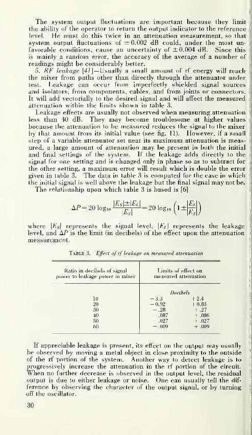
The system output fluctuations are important because they limit
the abihty of the operator to return the output indicator to the reference
level. He must do this twice in an attenuation measurement, so that
system output fluctuations of ±0.002 dB could, under the most un-
favorable conditions, cause an uncertainty of ±0.004 dB. Since this
is mainly a random error, the accuracy of the average of a number of
readings might be considerably better.
5. RF leakage [4i]— Usually a small amount of rf energy wiU reachthe mixer from paths other than directly through the attenuator undertest. Leakage can occur from imperfectly shielded signal sources
and isolators, from components, cables, and from joints or connectors.
It will add vectorially to the desired signal and will affect the measuredattenuation within the limits shown in table 3.
Leakage effects are usually not observed when measuring attenuation
less than 40 dB. They may become troublesome at higher values
because the attenuation to be measured reduces the signal to the mixerby that amount from its initial value (see fig. 11). However, if a small
step of a variable attenuator set near its maximum attenuation is meas-ured, a large amount of attenuation may be present in both the initial
and final settings of the system. If the leakage adds directly to the
signal for one setting and is changed only in phase so as to subtract for
the other setting, a maximum error will result which is double the error
given in table 3. The data in table 3 is computed for the case in whichthe initial signal is well above the leakage but the final signal may not be.
The relationship upon which table 3 is based is [6]
AP= 20 logio\Es\±\E,\
20 logio 1±
where \Es\ represents the signal level, \El\ represents the leakage '
level, and AP is the limit (in decibels) of the effect upon the attenuation
measurement.
Table 3. Effect of rf leakage on measured attenuation
Ratio in decibels of signal
power to leakage power in mixerLimits of effect on
measured attenuation
Decibels
10
2030405060
-3.3-0.92-.28-.087-.027-.009
f 2.4
^-0.83
+ .27
+ .086
+ .027
+ .009
If appreciable leakage is present, its effect on the output may usually
be observed by moving a metal object in close proximity to the outside
of the rf portion of the system. Another way to detect leakage is to
progressively increase the attenuation in the rf portion of the circuit.
When no further decrease is observed in the output level, the residual
output is due to either leakage or noise. One can usually tell the dif-
ference by observing the character of the output signal, or by turning
off^ the oscillator.
30

Perhaps the most sensitive method for detecting and locating sources
of leakage is to use an auxihary receiver having a cable and movable
probe or antenna. One explores the vicinity of joints and connectors
with the probe. At present, there are no really satisfactory methods
to measure or specify leakage from individual sources. Thus the re-
duction of leakage from a system is usually accomplished by a tedious
process of elimination which ends when the leakage effects are no
longer observed.
One method used to indicate a reduction of leakage is to record the
system output on a sensitive recorder. Output variations will result
from system instabilities and also from leakage fluctuations caused bymovement of personnel in the vicinity. When personnel movementhas no further effect on output variations (as determined by personnel
temporarily leaving the room), leakage is probably at least 20 dB belowsignal level.
It is usually necessary to place oscillators in shield cans, use gaskets
at joints, and to wrap leaking components with steel wool or metal mesh,when measuring high attenuations.
Errors caused by leakage can have both systematic and random com-ponents, but can be made more random by varying the phase of the leak-
age in some way from one measurement to another. One way wouldbe to make a number of measurements, each at a slightly different
frequency from the desired frequency. Also, a hne stretcher mightbe used to change the phase of the energy reaching the mixer via the
desired path through the attenuator.
6. IF leakage— heakage in the IF portion of the system is usually
not as bad a problem as in the rf portion. This is not because the loss
in the path is not as great, but because the openings which permitleakage are smaller compared to a wavelength. However, any IFleakage that does occur is usually more difficult to detect or ehminateand can cause errors at higher attenuations. It is also good practice
to reduce IF leakage so as to reduce interference from (or to) nearbysystems which may be operating at the same frequency.
7. Errors in standard attenuator— The errors in the standard attenua-
tor are basic and have been discussed previously in section 3.3. Ex-perience with various methods of attenuation measurement leads to the
I
conclusion that with sufficient refinement of design, construction, and
I
operation of the waveguide below cutoff attenuator, the uncertainty of
the average of five attenuation measurements can be less than 0.001dB at 20 dB. With Uttle or no refinement, the corresponding uncer-tainty could have been as much as 2.0 dB. This indicates that consider-
able attention must be paid to the waveguide below cutoff attenuation
I
standard if one is to have confidence in its calculated attenuation rate
given by eq (17).
[8. Noise— As long as the signal levels in the system are at least 10
jdB above the noise, as is usually the case, the noise does not contributesignificantly to uncertainties in attenuation measurement. However,when large attenuations are to be measured, one inserts a large amountof IF attenuation and sets the output signal to a reference level nearthe noise level. This noise may originate within the IF amplifier, the
,
mixer, the local oscillator, or the signal source.
|j
In the "straight" IF substitution system, the unknown and the stand-ard attenuators are varied so as to present the same signal level to theIF amplifier. Thus if the noise originates mainly within the IF ampli-
fier, there will be little effect on the measured attenuation other than to
decrease the resolution with which the reference level can be reset,
and thereby decrease the precision of the measurement. Systematic
effects have been noted [42] by some observers.
If the noise originates mainly within the mixer, it wiU have its greatest
effect on the output when the IF attenuator is set to the least attenua-
tion, and least effect when it is set to the greatest attenuation during
a measurement. In making a measurement of 20 dB 6r more, the ref-
erence level will be obtained from amplified signal and noise in one case,
and amplified signal in the other. Less signal wiU be required whennoise is present, so that the IF attenuation change will be less than the
rf change. The result is that the measured rf attenuation wiU be low.
If the noise originates mainly in the rf portion of the circuit, it will
tend to remain fairly steady as the rf attenuator varies and should have
a similar effect to noise originating within the mixer.
If noise originating within the local oscillator is troublesome, its
effect can be diminished by using a balanced mixer. As with audio
substitution, synchronous detection at the intermediate frequency can
reduce the effect of noise considerably.
9. Errors from connectors or waveguide joints and from waveguide or
cable— It was mentioned earlier (sect. 2.7) that the desired quantity in
an attenuation measurement is the substitution loss in a nonreflecting
system which is initially joined at the insertion point by a standard con-
nector pair or adapter. If the connector pair at the insertion point is
not standard, an error is introduced which has been analyzed [7]. This
error is normally less than 0.1 dB, for ordinary connectors and is probably
less than 0.01 dB for high-precision connectors.
Errors caused by slightly nonstandard waveguide at the insertion
point are difficult to assess, but have been experimentally found to benegligible (less than 0.001 dB) in practical cases.
Flexible cable or waveguide .is ordinarily not used at the insertion
point or elsewhere in the rf portion of the system. When flexed, the
phase shift through the cable changes and the interaction of reflections
may cause ampfitude changes large enough to result in serious errors.
Changes in the dissipative losses in the cable when flexed may causesimilar errors. At frequencies of approximately 100 MHz and below,loops of flexible cable are used to minimize flexing and these undesir-
able effects are largely avoided by this technique. However, at higher
frequencies it becomes increasingly difficult to avoid flexing effects.
Above approximately 6 GHz, leakage is such a serious problem that useof flexible cables is rare.
When the attenuation measurement requires the insertion and re-
moval of an attenuator, it is necessary to move a portion of the rf system
such as the local osciUator and mixer assembly. In order to facilitate
this motion, flexible cables are used in the IF and the d-c portions of
the circuit, where they ordinarily cause no trouble.
10. Errors associated with the device under test— The characteristics
of the device under test definitely affect certain sources of error in its
measurement. For example, mismatch error depends upon the reflec-
tions from the device under test. If we knew that the system had noreflections at all, the mismatch error according to eq (13) would vanish
regardless of the reflections from the device under test. In practice,
this is not the case, so that given the same system, lower hmits will be
32

obtained for the uncertainty of attenuation measurement of a device
having low reflections than for one having higher reflections.
A pad which is not stable, or has poor quaUty connectors, may have
a different loss each time it is measured. Similarly, a variable attenua-
tor may not be capable of repeating the same step in attenuation due to
mechanical defects or other difficulties. Unless these effects are noted,
the operator may mistakenly attribute them to his system rather than
to the device under test.
11. Overall error— It should be apparent that it is difficult to quote
reUable Umits for the uncertainty of attenuation measurements with a
given system. The quoted limits of error should vary with the amountof the attenuation being measured, gradually increasing at the extremeends of the range. Also, since the characteristics of the device undertest influence the errors, limits on these characteristics should be
quoted.
In some cases, the uncertainty Umits quoted for calibrating attenu-
ators are sufficiently conservative so that they are seldom exceeded.
In other cases, it is implied, but not stated, that the devices under test
must meet certain requirements and have certain characteristics.
It appears that the best way to compare diff^erent attenuation measure-ment systems is to use them to measure the same attenuators at the
same frequency and under similar conditions. This has the disadvan-
tage that similar systematic errors in the systems will not be revealed.
For this reason, confidence in an attenuation measurement system canbe increased by comparing measurements [43] of the same attenuators
in systems having different systematic errors.
5.5. Modulated Subcarrier
The modulated subcarrier technique [44, 45] bears marked similarity
to in IF substitution technique in which the signal source and the local
oscillator operate at the same frequency and the signal source alone is
amplitude modulated. The signals combine in a mixer and producean output at the modulation frequency. The power conversion is verynearly hnear over wide ranges of attenuation, as in the IF substitution
technique, and the standard attenuator operates at the modulationfrequency.
Actually one signal source is used, and its unmodulated output is
spht and fed to two channels as shown in figure 12. The channelcontaining the device under test is modulated and the modulator also
excites a standard attenuator. The signals from the two channelsare combined and fed to a phase sensitive detector which also receives
a signal from the standard attenuator at the modulation frequency.In this version of the system, a detector null is obtained which dependsupon phase and amplitude relationships at the modulation frequency.The modulated subcarrier technique has the following advantages
over the IF substitution technique: (1) only one signal source is re-
quired, (2) satisfactory audio attenuation standards are commerciallyavailable at relatively low cost, (3) the phase shift of the device undertest may be determined at the same time that its attenuation is beingmeasured, and (4) a higher resolution is obtained at low attenuations.
The following disadvantages tend to "balance the scales": (1) the
procedure in making a measurement is less convenient: (2) the range
33
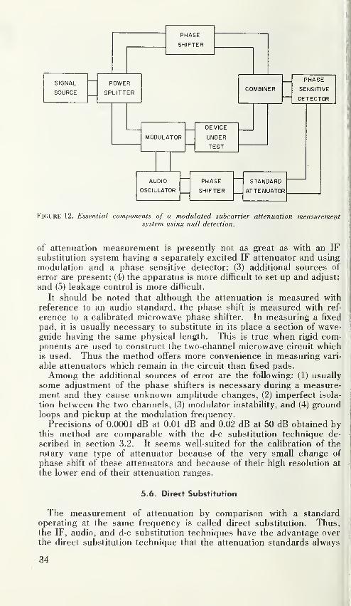
1
PHASE
SHIFTER
SIGNAL
SOURCE
POWER
SPLITTER
MODULATOR
AUDIO
OSCILLATOR
PHASE
SHIFTER
COMBINER
DEVICE
UNDER
TEST
PHASE
SENSITIVE
DETECTOR
STANDARD
ATTENUATOR
Figure 12. Essential components of a modulated subcarrier attenuation measurementsystem using null detection.
of attenuation measurement is presently not as great as with an IFsubstitution system having a separately excited IF attenuator and using
modulation and a phase sensitive detector; (3) additional sources of
error are present; (4) the apparatus is more difficult to set up and adjust;
and (5) leakage control is more difficult.
It should be noted that although the attenuation is measured with
reference to an audio standard, the phase shift is measured with ref-
erence to a calibrated microwave phase shifter. In measuring a fixed
pad, it is usually necessary to substitute in its place a section of wave-guide having the same physical length. This is true when rigid com-ponents are used to construct the two-channel microwave circuit whichis used. Thus the method offers more convenience in measuring vari-
able attenuators which remain in the circuit than fixed pads.
Among the additional sources of error are the following: (1) usually
some adjustment of the phase shifters is necessary during a measure-ment and they cause unknown amphtude changes, (2) imperfect isola-
tion between the two channels, (3) modulator instability, and (4) groundloops and pickup at the modulation frequency.
Precisions of 0.0001 dB at 0.01 dB and 0.02 dB at 50 dB obtained bythis method are comparable with the d-c substitution technique de-
scribed in section 3.2. It seems well-suited for the calibration of the
rotary vane type of attenuator because of the very small change of
phase shift of these attenuators and because of their high resolution at
the lower end of their attenuation ranges.
5.6. Direct Substitution
The measurement of attenuation by comparison with a standardoperating at the same frequency is called direct substitution. Thus,the IF, audio, and d-c substitution techniques have the advantage overthe direct substitution technique that the attenuation standards always
34

operate at a fixed frequency, no matter what frequency is chosen for
the attenuator calibration. However, the direct substitution technique
has other advantages, such as increased range. Three direct substi-
tution arrangements are shown in figure 13.
The parallel substitution arrangement of figure 13(a) is often usedbecause it offers high resolution and range, and tolerates more amph-tude instabihty of the signal source. It does require adjustment of a
phase shifter which ideally should have an unchanging loss during these
adjustments.
One should not confuse this parallel substitution arrangement with
that of figure 11(c), which has been called [24] parallel IF substitution.
SIGNAL
SOURCE
STANDARD
ATTENUATOR
PHASE
SHIFTER
POWER
SPLITTER
(a)
COMBINER
DEVICE
UNDER
TEST
DETECTOR
(bl
DEVICE
UNDERSIGNAL STANDARD
DETECTORSOURCE ATTENUATOR
TEST
SIGNAL
SOURCE
PHASE
SHIFTER
POWER
SPLITTER
(C)
COMBINER
STANDARD
ATTENUATOR
DEVICE
UNDER
TEST
DETECTOR
"IGURE 13. Basic arrangements for the measurement ofattenuation using direct substitution.
(a) Parallel
(b) Series
(c) Combination
35

The parallel substitution arrangement is well suited to use with wave-j
guide-below-cutoff attenuators which have a high residual attenuation ,
and very little change of phase shift.j
The series substitution arrangement is often used when an attenuatorf
is calibrated with reference to a standard attenuator built into a stand-
ard signal generator. It is also used to extend the range of IF substitu-
tion systems. It is very convenient and requires no phase shifters.
However, it introduces additional loss between the signal source andthe detector. For this reason, it is weU-suited for use with the rotary
j
vane attenuator which has small residual attenuation.
The combination arrangement [18k] has also been used for a widerange, high-precision, fixed-frequency system.
In addition to the waveguide-below-cutofif and the rotary vane types
of attenuators, other attenuation standards have been used with direct
substitution systems. For example, a short-circuited slotted line ideallyi
has a sinusoidal voltage standing wave. One can then vary the outputof the traveling probe in a predictable manner and calculate the relative
output from the measured probe displacement relative to a minimumposition. An arrangement for doing this is shown in figure 14(a). Asone approaches a mimimum, the probe response departs from the sinus-
DETECTOR
SIGNAL
SOURCE
VOLTAGE STANDING WAVE
PROBE
DEVICE
UNDER
TEST(a)
PLANE REFLECTOR
SIGNAL
SOURCE
„_DEVICE
UNDER
TESTDETECTOR (b)
Figure 14. Standard attenuators for direct substitution attenuation measurements.
(a) short-circuited slotted line
lb) rotating dipole in plane polarized field
36

oidal distribution due to line losses. However, a practical range of
5 to 15 dB is possible. Near the maximum, the response is closest to
sinusoidal. The variation of probe coupUng vyrith travel is within 0.5
percent or 0.04 dB in a slotted line of high quality.
Another standard of attenuation for direct substitution consists of a
rotating dipole antenna in a linearly polarized field, as shown in figure
14{b). The probe response is ideally proportional to the cosine of theangle 6 between the dipole and the f'-field. Hence, relative levels canbe predicted given the angular position of the dipole relative to the^-field.
5.7. Short-Circuited Attenuator [46]
The wave traveling through an attenuator and reflected by a short-
circuit is attenuated twice before it reaches the input and becomes the
reflected wave. Thus the reflection coefficient Y at the input to a short-
circuited attenuator should have a magnitude
where a is the attenuation in nepers. (IfA is the attenuation in decibels,
A = 8.686a.) Thus a short-circuited 20 dB pad should have an input
reflection coefficient of 0.01, or a VSWR of 1.02. This assumes that the
attenuator introduces no additional reflections. If this were generally
true, it would be possible to determine the attenuation by measuringthe VSWR of a short-circuited pad.
Unfortunately, attenuators usually produce internal reflections whichare large enough to cause serious errors if the above procedure werefollowed. However, it is stiU possible to determine attenuation in
terms of the input reflection coefficients of a short-circuited pad, the
short-circuit being a shding short-circuit in a section of waveguide.
Using a two-port network as a model for the attenuator, and assumingthat Zoi = Zo2 it is known that the attenuation A is
^ = 10 logio |5~~|2"" 10 loglO|g
+1Q logio|2
, (22)
where the two components are those due to dissipation and to reflection
of energy, respectively, and it is assumed that energy enters port 1
and leaves port 2.
It is also known that the reflection coefficient F-z is
where Tt is the reflection coefficient of a load terminating port 1, andthe signal source is connected to arm 2.
If the phase of F/, is varied, while \Tl\ remains constant, the locus ofr2 is a circle of radius
i-|5„r/j2 (^4)
37
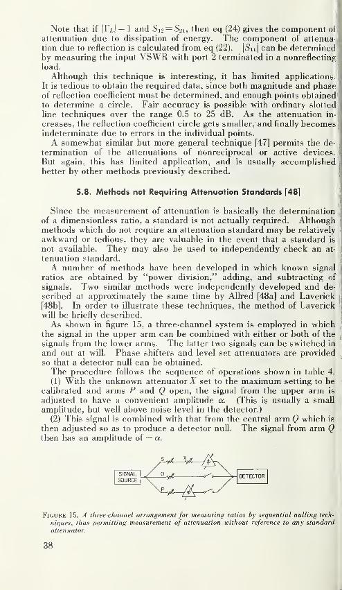
Note that if IF/J = 1 and Si2 = S2i, then eq (24) gives the component of
attenuation due to dissipation of energy. The component of attenua-i
tion due to reflection is calculated from eq (22). |Sii|
can be determinedby measuring the input VSWR with port 2 terminated in a nonreflecting
load.
Although this technique is interesting, it has limited applications.
It is tedious to obtain the required data, since both magnitude and phaseof reflection coefficient must be determined, and enough points obtainedto determine a circle. Fair accuracy is possible with ordinary slotted
line techniques over the range 0.5 to 25 dB. As the attenuation in-
creases, the reflection coefficient circle gets smaller, and finally becomesindeterminate due to errors in the individual points.
A somewhat similar but more general technique [47] permits the de-
termination of the attenuations of nonreciprocal or active devices.
But again, this has limited application, and is usually accompfishedbetter by other methods previously described.
5.8. Methods not Requiring Attenuation Standards [48]
Since the measurement of attenuation is basically the determinationof a dimensionless ratio, a standard is not actually required. Althoughmethods which do not require an attenuation standard may be relatively
awkward or tedious, they are valuable in the event that a standard is
not available. They may also be used to independently check an at-
tenuation standard.
A number of methods have been developed in which known signal,
ratios are obtained by "power division," adding, and subtracting of
signals. Two similar methods were independently developed and de-
scribed at approximately the same time by AUred [48a] and Laverick
[48b]. In order to illustrate these techniques, the method of Laverickwill be briefly described.
As shown in figure 15, a three-channel system is employed in whichthe signal in the upper arm can be combined with either or both of the
signals from the lower arms. The latter two signals can be switched in
and out at will. Phase shifters and level set attenuators are provided
so that a detector null can be obtained.
The procedure follows the sequence of operations shown in table 4.
(1) With the unknown attenuator^ set to the maximum setting to becalibrated and arms P and Q open, the signal from the upper arm is
adjusted to have a convenient ampUtude a. (This is usually a small
amplitude, but well above noise level in the detector.)
(2) This signal is combined with that from the central arm Q which is
then adjusted so as to produce a detector null. The signal from arm Qthen has an amplitude of — a.
DETECTOR
Figure 15. A three-channel arrangement for measuring ratios by sequential nulling tech-
niques, thus permitting measurement of attenuation without reference to any standard
attenuator.
38

Table 4. Signal amplitudes in each channel in successive operations in Laverick's
cedure for calibrating an attenuator
Chan-nel
Step 1 Step 2 Step 3
Etc.
1 2 3 4 5 1 2 3 1 2 3
SPQ
a a
— a
a— a
a— a— a
2a— a— a
2a-2a
2(
-2a— a
3a-2a— a
3a-3a
3a-3a— a
4a-3a— Q
Etc.
(3) With arm Q open, the signal from arm S is combined with that fromthe lower arm P. Arm P is then adjusted so as to produce a detectornuU. The signal from arm P then has an amplitude of — a.
(4) The signals from all three channels are then combined.(5) The attenuator X to be calibrated in arm S is adjusted for a de-
tector nuU. (Some adjustment of the phase shifter in arm S may also
be required, but it is assumed that this causes negligible change in thesignal amplitude.)
This completes step 1.
It is clear that the attenuator adjustment changed the amplitude of
the signal of arm S from a to 2a, and thus produced an attenuation
change of 6.02 dB. In the subsequent steps, as shown in table 4, channel
Q is not adjusted, but channel P is adjusted each time to balance chan-nel S. Then, all three channels are combined so that the attenuator Xmust be changed a known amount to restore the detector null. Thecorresponding attenuation steps are 6.0206, 3.5218, 2.4988 dB, etc.,
as shown in table 5. The attenuator under test must be initially set
at a fairly large dial reading, say 20 dB, since each step in the aboveprocedure reduces its attenuation by a certain amount. Intermediatepoints can then be obtained by starting over again with a different
initial setting of the test attenuator.
It is apparent that even though no attenuation standard is used, there
are a number of sources of error present. For example, there are mis-
TaBLE 5. Magnitude of amplitude ratio expressed in decibels for successive steps in thecalibration of an attenuator by Laverick's procedure
Magnitude of ratio of Incremental TotalStep amplitude change in attenuation change attenuation change
channel S in decibels in decibels
1 2 6.0206 6.02062 3/2 3.5218 9.54243 4/3 2.4988 12.04124 5/4 1.9382 13.97945 6/5 1.5836 15.56306 7/6 1.3390 16.90207 8/7 1.1598 18.06188 9/8 1.0230 19.08489 10/9 0.9152 20.000010 11/10 0.8278 20.8278
39

match errors caused by system reflections at the place where the test
attenuator is inserted, changes in power division between channelscaused by changes in reflection, changes in level caused by readjust-
ments of phase shifters, and changes in level caused by frequencydrift. There is also a small error each time that the signal in any chan-
nel is adjusted to produce a detector null, due to the limited resolution
of this process. This error depends upon the sensitivity of the detector,
repeatabilities of the attenuators, and noise level, and has a cumulativeeffect as more and more steps are taken. The procedure is not as
convenient to use as methods which employ standard attenuators.
However, if no standard is available, the method can be used, and withcare, uncertainties of less than 0.02 dB in measurements of up to 20 dBcan be achieved.
This method is weU-suited for the calibration of variable attenuators
which do not produce large changes in phase shift. Laverick has usedthe method for the calibration of rotary vane attenuators in rectangular
waveguide, and AUred has calibrated waveguide-below-cutoflf attenua-
tors in coaxial systems. When such an attenuator is used as a standardin an intermediate frequency substitution method for attenuation
measurement, confidence in the standard may be increased by cahbrat-
ing it as AUred has done. In addition, he has shown how a measure-ment of the phase shift of the attenuator may also be made.
Several other methods not requiring a standard attenuator have beendescribed by Peck [48c] and Davies [48d]. One of the methods [48c]
makes use of a detector whose response varies linearly with the magni-tude of the signal amplitude (a linear voltmeter, for example). A graphi-
cal method is used to eliminate the constants in the linear relationship,
and the accuracy of the results is limited by the linearity of the detector
and the precision of the graphical analysis.
This method is modified by using two- and three-channel nulling
arrangements in which the dependence on detector linearity is elimi-
nated, and the detector serves only as a null indicator. An interesting
test of these methods was described by Peck. A waveguide-below-cutoff attenuation standard was "calibrated" by several methods andthe results compared with the attenuation rate of 10.000 ±0.002 dB perinch predicted from design data. Using three versions of his method,the following results were obtained: 10.006, 10.003, and 10.023 dB perinch. The discrepancy of approximately 0.02 dB per inch was ascribed
to reflection interactions in the system.The method described by Davies [48d] makes use of two identical
3-dB directional couplers and employs a two-channel circuit, nulling
the demodulated outputs. Thus adjustable phase shifters are not re-
quired. The accuracy is claimed to be 1 percent of the attenuation in
decibels, in contrast to Laverick's estimate of 0.1 percent.
5.9. Measurement of Small Attenuation
The measurement of smaU attenuation is of interest in the determin-
ation of losses in short sections of waveguide, and other low-loss com-ponents.
A number of methods are based upon the measurement of the VSWRof a short-circuited section of waveguide [49a, b].
40
Another method [49c] measures the loss of a transmission cavity con-structed of the waveguide sample and two irises. The loss of each ofthe irises must be evaluated. Although not claimed to be highly accu-rate, the method is ver\- convenient to use. The low loss is measuredwith reference to a rotary vane attenuator.
Methods having high resolution have been developed using a two-channel arrangement with nulling of audio or d-c signals after detection[49d, e]. They are inexpensive and convenient to use.
Another method having high resolution and accuracy uses a two-channel arrangement in which a null is obtained with a phase shifter
and attenuator [49f]. Errors are reduced by use of a quarter-wavelengthshort-circuit and the selection of a frequency at which the length of thesample is effectively a half wavelength. Then no change in the phaseshifter is required to restore the null. A rotary vane attenuator is usedas a standard and a precision of 0.001 dB is obtained.
Direct substitution techniques are also used, but require exceptionallyhigh stabihty of the signal source and detector.
6. Conclusions
Many methods are available to measure attenuation. The currentstate of the art can be inferred from articles in the hterature [50]. It
can be measured without reference to an attenuation standard. How-ever, methods which employ an attenuation standard are more conven-ient to use.
At present, the claim of highest accuracy is ±0.0001 dB at 0.01 dB,using d-c substitution techniques. At 30 MHz, a range of 150 dB is
obtained in a series-parallel substitution arrangement using a wave-guide-below-cutoff attenuator of high accuracy. Somewhat greaterranges are obtainable from signal generators, but accuracy is ±2 dB.The rotary vane attenuator shows promise as a standard attenuator.
However, refinements and the analysis of errors are currently underway.The rotary vane attenuator will probably be used as a standard of attenua-
tion in IF substitution systems operating at 0.1 to 10 THz. At higherfrequencies, prisms, polarizers-analyzers, and other optical techniqueswiU probably take over.
The above material has evolved as a result of two courses presentedat NBS over the past several years. One was entitled Microwave Meas-urements and the other was the RSL Summer Course in ElectromagneticMeasurements. The author has consulted notes prepared for thesecourses by C. M. Allred and G. E. Schafer of NBS, as well as textbookmaterial by numerous other authors [51]. In addition, considerableinformation arising out of the author's own experience is presented.Helpful discussions on attenuation measurements and standards havebeen held with a number of NBS personnel, including D. A. Ellerbruch,W. Larson, W. E. Little. A. Y. Rumfelt. and D. H. RusseU. The verythorough review of this manuscript by C. C. Cook was especially valu-
able. References to work pubhshed in the hterature may not actually
be complete but are fairly extensive.
41
7. References
[1] IRE standards on antennas and waveguides: Definitions of terms, Proc. IRE 41,No. 12, 1721-1728, Standard 53 IRE 2.S1, 1953.
[2] R. W. Beatty, Insertion loss concepts, Proc. IEEE 52, 663-671 (June 1964).
[3] R. W. Beatty, The system of electromagnetic quantities at frequencies above 1 GHz,Metrologia 2, 46-54 (Jan. 1966).
[4] I. A. Harris, Mode of use and assessment of precision coaxial connectors, Proc.
lEE (London) 112, 2025-2032 (Nov. 1965).
[5] By adapting eq (2.50) of Basic Theory of Waveguide Junctions and Introductory Micro-
wave Network Analysis, David M. Kerns and Robert W. Beatty, Pergamon Press,New York, N.Y., May 1967, one can write
,p Pg2.l^(l-|T,P)'•
Z„, |(l-'S„Tf;)(l-'S,,T,,)-'-S„'S„Tr.T,,|2
It follows that the ratio of 'P,, to ^Pi, is
' 1-|T,.|2 il-fSnJTa)(l-rS2/r,)
i-Kr,.|^ (i-'S,,T,;)(i-'S..'n,)
and eq (3) then follows from substitution of the ratio of 'P;, to Vi. into eq (1).
[6] See for example Ernst Weber, The measurement of attenuation, in Technique of
Microwave Measurements, Sect. 13.5, Ch. 13, MIT Rad. Lab. Series 11, McGraw-Hill Book Co., Inc., New York, N.Y., 824-832 (1947).
[7] R. W. Beatty, Effects of connectors and adapters on accurate attenuation measure-ments at microwave frequencies, IEEE Trans. Instr. 13, 272-284 (Dec. 1964).
[8] R. W. Beatty, Mismatch errors in the measurement of ultrahigh-frequency and micro-
wave variable attenuators, J. Res. NBS 52. 7-9 (Jan. 1954).
[9] G. E. Schafer and A. Y. Rumfelt, Mismatch errors in cascade-connected variable
attenuators, IRE Trans. MTT 7, 447-453 (Oct. 1959).
[10] K. Tomiyasu, Intrinsic insertion loss of a mismatched microwave network, IRE Trans.
MTT 3, 40-44 (Jan. 1955).
[11] R. W. Beatty, Intrinsic attenuation, IEEE Trans. MTT 11, 179-182 (May 1963).
[12] H. M. Altschuler and W. K. Kahn, Nonreciprocal two-ports represented by modified
.Wheeler networks. IRE Trans. MTT 4, 228-233 (Oct'. 1956).
[13] Andrew F. Dunn, Calibration of a Kelvin-Varley voltage divider, IEEE Trans. Instr.
Meas. 13, 129-139 (June-Sept. 1964).
[14] Walter J. Karplus, Design and error analysis of high-accuracy DC voltage-measuring
systems, IEEE Trans. Instr. Meas. 13, 139-145 (June-Sept. 1964).
[15] Thomas L. Zapf, Voltage ratio measurements with a transformer capacitance bridge,
J. Res. NBS 66C, 25-32 (Jan.-Mar. 1962).
[16] T. L. Zapf, The accurate measurement of voltage ratios of inductive voltage dividers,
Acta IMEKO III, 317-331 (1964).
[17] J. S. Elliott, Coaxial attenuation standards, Bell Labs. Record 27, 221-225 (June 1949).
[18] Selected bibliography on waveguide-below-cutoiT attenuators:
a. D. E. Harnett and N. P. Case, The design and testing of multirange receivers,
Proc. IRE 23, 578-593 (June 1935).
b. R. N. Griesheimer,^ Microwave attenuators. Cutoff attenuators. Technique of
microwave measurements, Ch. 11, MIT Rad. Lab. Series, 11, McGraw-Hill
Book Co., Inc., New York, N.Y., 685-719 (1947).
c. G. F. Gainsborough, A method of calibrating standard-signal generators and radio-
frequency attenuators, J. IEEE (London) 94, Pt. Ill, 203-210 (May 1947).
d. J. J. Freeman, Theory and design of a cavity attenuator, J. Res. NBS 40, 235-243
(Mar. 1948).
e. R. E. Grantham and J. J. Freeman, A standard of attenuation for microwave meas-
urements. Trans. AIEE 67, 329-335 (June 1948).
f. H. A. Wheeler, The piston attenuator in a waveguide below cutoff. Wheeler Mono.No. 8 (Jan. 1949).
g. J. Brown, Corrections to the attenuation constants of piston attenuators, Proc.
lEE (London) 96, Pt. Ill, 491-495 (Nov. 1949).
h. H. M. Barlow and A. L. CuUen, Microwave measurements, Constable and Co.,
Ltd., London, England, 242-254, 384-388 (1950).
42
i. CM. AUred, Chart for the TE„ mode piston attenuator, J. Res. NBS 48, 109-110(Feb. 1952).
j. D. M. Kerns and R. W. Hedberg, Propagation constant in rectangular waveguideof finite conductivity, J. Appl. Phys. 25, 1550-1551 (Dec. 1954).
k. C. M. Allred and C. C. Cook, A precision RF attenuation calibration system,
IRE Trans. Instr. 9, 268-274 (Sept. 1960).
1. L. A. Birger, Nonlinearity of cutoff attenuators due to the effect of loading, Izm.
Tekh. No. 11, 59-61 (1960).
m. D. L. Hollway and F. P. Kelly, A standard attenuator and the precise measurementof attenuation, lEE Trans. Instr. Meas. 13, 33-44 (Mar. 1964).
n. B. O. Weinschel and G. U. Sorger, Waveguide below cutoff attenuation standard,
Acta IMEKO III, 407-424 (1964).
[19] Selected bibliography on the rotary vane attenuator:
a. G. C. Southworth, Principles and Applications of Waveguide Transmission, D.
Van Nostrand Co., Inc., New York, N.Y. 374-376 (1950).
b. B. P. Hand, A precision waveguide attenuator which obeys a mathematical law,
Hewlett-Packard Journal 6, 1-2 (Jan. 1955).
c. Wilbur Larson, Analysis of rotation errors of a waveguide rotary vane attenuator,
IRE International Convention Record, Pt. 3, 213-219 (1962).
d. P. F. Mariner, An absolute microwave attenuator, Proc. lEE (London) 109, Pt. B,
415-419 (Sept. 1962).
e. Allan V. James, A high-accuracy microwave-attenuation standard for use in pri-
mary calibration laboratories, IRE Trans. Instr. 11, 285-290 (Dec. 1962).
f. Wilbur Larson, Table of attenuation error as a function of vane-angle error for
rotary vane attenuators, NBS Tech. Note No. 177 (May 1963).
g. Wilbur Larson, Gearing errors as related to alignment techniques of the rotary
vane attenuator, IEEE Trans. Instr. Meas. 14, 117-123 (Sept. 1965).
h. Wilbur Larson, Table of attenuation as a function of vane angle for rotary-vane
attenuators (/i =-40 log,o cos 6), NBS Tech. Note No. 229 (Jan. 7, 1965).
j
[20] G. F. Engen and R. W. Beatty, Microwave attenuation measurements vvith accuracies
from 0.0001 to 0.06 decibel over a range of 0.01 to 50 decibels, J. Res. NBS 64C,139-145 (Apr. -June 1960).
[21] R. W. Beatty and C. E. Huber, Lossy cable attenuator pads. Rev. Sci. Instr. 24,1002-1003 (Oct. 1953).
I [22] B. O. Weinschel, Card attenuator for microwave frequencies, U.S. Patent No. 3,157,846
j
(17 Nov. 1964).
[23] Wilbur Larson, Inline waveguide attenuator (correspondence), IEEE Trans. MTT 12,'! 367-368 (May 1964).
I
[24] B. O. Weinschel, An accurate attenuation measuring system with great dynamicrange. Microwave J. 4, 77-83 (Sept. 1961).
(i[25] Glenn F. Engen, Recent developments in the field of microwave power measurementsj,
at the National Bureau of Standards, IRE Trans. Instr. 7, 304-306 (Dec. 1958).
J[26] John Korewick, A-M System measures microwave attenuation. Electronics 27,J 175-177 (Jan. 1954).
|[27] G. U. Sorger and B. O. Weinschel, Comparison of deviations from square law for RF' crystal diodes and barretters, IRE Trans. Instr. 8, 103-111 (Dec. 1959).
j[28] G. F. Engen, A DC-RF substitution error in dual-element bolometer mounts, IEEETrans. Instr. Meas. 13, 58-64 (June-Sept. 1964). (It is noted that the substitution
error varies with power level.)
[29] Square-law microwave detector. Military Sys. Design 6, 58 (Sept.-Oct. 1962).
i[30]G. B. Bogdanov, Possible application of ferrites for absolute measurement of micro-
i wave power (Radiotekhnika i Elektronika, 4, 663 (1961)). Radio Engineering and
|.Electronic Physics 4, 587 (1961).
|[31] F. L. Wentworth, J. D. Rodgers, J. W. Dozier, and M. Cohn, Millimeter wave harmonic' generators, mixers, and detector. Program and Digest, The Millimeter and Sub-
millimeter Conference. (Copies available from E. D. Houseman, MP-75, Martin
j
Co., Orlando, Florida) 103-105 (1963).
il[32] S. Hopfer, N. H. Riederman, and L. Nadler, The properties of thermoelectric elements
I
as microwave power detectors, IRE Intern. Convention Record, Pt. 3, 77-84 (1962).
I[33] G. U. Sorger and B. O. Weinschel, Precise insertion loss measurements using imper-
f feet square law detectors and accuracy limitations due to noise, IRE Trans. Instr.
4, 55-68 (Oct. 1955).
[34] The Microwave Engineer's Handbook and Buyer's Guide, 318-319 (1966).
[35] R. W. Beatty, Cascade-connected attenuators, J. Res. NBS 45, 231-235 (Sept. 1950).
.i[36] A. N. Leber, Method free from mismatching errors for measuring the loss of attenu-
ators (Correspondence), IEEE Trans. MTT 12, 480 (July 1964).
43

[37] F. E. Terman, Radio Engineering, McGraw-Hill Book Co., Inc., New York, N.Y., 2d ed.,
448-449 (1937).
[38] B. 0. Weinschel, G. U. Sorger, and A. L. Hedrich, Relative voltmeter for VHF/UHFsignal generator attenuator calibration IRE Trans. Instr. 8, 22-31 (Mar. 1959).
[39] E. Niesen, R. W. Beatty, and W. J. Anson, Water-cooling of low-power klystrons used
in the laboratory. Rev. Sci. Instr. 29, 791-792 (Sept. 1958).
[40] Wilbur Anson and Edward Niesen, Fast melting alloy forms water jacket for small
klystrons, Micro Waves 42 (Mar. 15, 1962).
[41] A good discussion is given on pp. 830-831 of reference 6.
[42] See pp. 845-846 of reference 6.
[43] Comparison of two techniques for measuring microwave attenuation. NBS Tech.
News Bull. 44, 192-193 flNov. 19'60).
[44] G. E. Schafer and R. R. Bowman, A modulated sub-carrier technique of measuring
microwave attenuation, Proc. lEE (London) 109, Pt. B, Suppl. No. 23, 783-786
(May 1962).
[45] William E. Little, Further analysis of the modulated subcarrier technique of attenua-
tion measurement, IEEE Trans. Instr. Meas. 13, 71-76 (June-Sept. 1964).
[46] R. W. Beatty, Determination of attenuation from impedance measurements, Proc.
IRE 38, 895-897 (Aug. 1950).
[47] H. M. Altschuler, The measurement of arbitrary linear microwave two-ports, Proc.
IFF (London) 109. Pt. B, Suppl. No. 23; 704-712 (May 1962).
[48] Selected bibliography on measurement of attenuation without using a standard:
a. Self-calibrating method of measuring insertion ratio, NBS Tech. News Bull. 41,132-133 (Sept. 1957).
b. E. Laverick, The calibration of microwave attenuators by an absolute method,
IRE Trans. MTT 4, 250-254 (Oct 1957).
c. R. L. Peck, A method for the self-calibration of attenuation-measuring systems,
J. Res. NBS 66C, 13-18 (Jan.-Mar. 1962).
d. M. C. Davies, An absolute method for calibrating microwave attenuators, Proc.
lEE (London) 109, Pt. B, Suppl. No. 23, 796-800 (May 1962).
[49] Selected bibhography on the measurement of small attenuations:
a. W. T. Blackband and D. R. Brown, The two-point method of measuring character-
istic impedance and attenuation of cables at 3000 Mc/s, J. lEE, Pt. IIIA, 93,i
1383-1386(1946). '
b. J. H. Vogelman, Precision measurement of waveguide attenuation, Electronics 26,|
196-199 (Dec. 1953).
c. Peter D. Lacy and Kenneth E. Miller, An improved method for measuring losses
in short waveguide lengths, Hewlett-Packard J. 9 (Nov. -Dec. 1957).
d. B. O. Weinschel, Insertion loss test sets using square law detectors, IRE Trans,j
Instr. 4, 160-164 (Oct. 1955).
e. C. T. Stelzried and S. M. Petty, Microwave insertion loss test set (correspondence),
IEEE Trans. MTT 12, 475-477 (July 1964).
f. R. W. Beatty, A two-channel nuUing method for measuring attenuation constants
of short sections of waveguide and the losses in waveguide joints (correspond-
ence), Proc. IEEE 53, 642-643 (June 1965).
[50] The current state of the art in attenuation standards can be inferred from manufac-
turer's literature and from articles in the literature such as the following:
a. R. E. Larson, Microwave measurements in the NBS electronic calibration center,
Proc. lEE (London) 109, Pt. B, Suppl. No. 23, 644-650 (May 1962).
b. R. W. Beatty, Standards and measurements of attenuation, impedance, and phase
shift, September 1960-December 1962 (URSI USA National Committee Report,
XlVth General Assembly, 1963), Radio Science J. Res. NBS/USNC-URSI 68D,529-533 (May 1964).
c. R. W. Beatty, Microwave standards and measurements, A progress review 1960-
1963, IEEE Trans. Instr. Meas. 12, 134-138 (Dec. 1963). Also see the book
Progress in Radio Science, 1960-1963, Vol. I. Radio Standards and Measure-
ments, Elsevier Publ. Co., Amsterdam, 1965. Articles in this book by D. Woods,S. Okamura and K. Sakurai, D. L. HoUway, and others discuss attenuation
measurements.d. Engineering Division, Radio Standards Laboratory, National Bureau of Standards,
Microwave and high-frequency calibration services of the National Bureau of
Standards, part II (correspondence), IEEE Trans. MTT 12, 572-576 (Sept. 1964).
e. W. A. Wildhack, R. C. Powell, and H. L. Mason (editors). Accuracy in measure-
ments and cahbrations, 1965, NBS Tech. Note 262 (June 15, 1965).
f. J. E. Ebert and G. U. Sorger, Survey of precision microwave attenuation measuring
techniques, ISA Trans. 3, 280-290 (July 1964).
44
1 [51] The following textbooks contain valuable source material on microwave attenuation
measurements and standards.
a. C. G. Montgomer>' (editor). Technique of Microwave Measurements. MIT Rad.
Lab. Series 1 1,'McGraw-HiU Book Co., Inc., New York, N.Y.. 1947. (See part
IV. beginning on p. 679.1
b. Donald D. King. Measurements at Centimeter Wavelength. D. Van Nostrand Co.,
Inc.. New York. N.Y.. 1952. (See sect. 3.13 beginning on p. 99.)
c. E. L. Ginzton. Microwave Measurements. McGraw-Hill Book Co., Inc., New York,
N.Y.. 1957. (See ch. 11. beginning on p. 462.)
d. Sucher & Fox (editors). Handbook of Microwave Measurements. 3d ed.. Poly-
technic Press. Pohtechnic Institute of BrooklvTi. Brooklyn, N.Y.. 1963. (See
ch. VII. beginning in vol. I. p. 377.1
45


U.S. DEPARTMENT OF COMMERCEWASHINGTON, D.C. 20230
POSTAGE AND FEES PAIDU.S. DEPARTMENT OF COMMERCI
OFFICIAL BUSINESS
t