microstructural dependence of the compressive mechanical
TRANSCRIPT
ARL-TR-8512 ● SEP 2018
US Army Research Laboratory
Microstructural Dependence of the Compressive Mechanical Response of Human Skull by Stephen L Alexander, C Allan Gunnarsson, Karin Rafaels, and Tusit Weerasooriya Approved for public release; distribution is unlimited.

NOTICES
Disclaimers
The research reported in this document was performed in connection with contract/instrument W911QX-16-D-0014 with the U.S. Army Research Laboratory. The views and conclusions contained in this document are those of SURVICE Engineering Company and the U.S. Army Research Laboratory. Citation of manufacturer’s or trade names does not constitute an official endorsement or approval of the use thereof. The U.S. Government is authorized to reproduce and distribute reprints for Government purposes notwithstanding any copyright notation hereon. The findings in this report are not to be construed as an official Department of the Army position unless so designated by other authorized documents. Destroy this report when it is no longer needed. Do not return it to the originator.

ARL-TR-8512 ● SEP 2018
US Army Research Laboratory
Microstructural Dependence of the Compressive Mechanical Response of Human Skull by Stephen L Alexander SURVICE Engineering Company, Belcamp, MD C Allan Gunnarsson, Karin Rafaels, and Tusit Weerasooriya Weapons and Materials Research Directorate, ARL Approved for public release; distribution is unlimited.
ii
REPORT DOCUMENTATION PAGE Form Approved OMB No. 0704-0188
Public reporting burden for this collection of information is estimated to average 1 hour per response, including the time for reviewing instructions, searching existing data sources, gathering and maintaining the data needed, and completing and reviewing the collection information. Send comments regarding this burden estimate or any other aspect of this collection of information, including suggestions for reducing the burden, to Department of Defense, Washington Headquarters Services, Directorate for Information Operations and Reports (0704-0188), 1215 Jefferson Davis Highway, Suite 1204, Arlington, VA 22202-4302. Respondents should be aware that notwithstanding any other provision of law, no person shall be subject to any penalty for failing to comply with a collection of information if it does not display a currently valid OMB control number. PLEASE DO NOT RETURN YOUR FORM TO THE ABOVE ADDRESS.
1. REPORT DATE (DD-MM-YYYY)
September 2018 2. REPORT TYPE
Technical Report 3. DATES COVERED (From - To)
August 2016–February 2018 4. TITLE AND SUBTITLE
Microstructural Dependence of the Compressive Mechanical Response of Human Skull
5a. CONTRACT NUMBER
5b. GRANT NUMBER
5c. PROGRAM ELEMENT NUMBER
6. AUTHOR(S)
Stephen L Alexander, C Allan Gunnarsson, Karin Rafaels, and Tusit Weerasooriya
5d. PROJECT NUMBER
5e. TASK NUMBER
5f. WORK UNIT NUMBER
7. PERFORMING ORGANIZATION NAME(S) AND ADDRESS(ES)
US Army Research Laboratory ATTN: RDRL-WMP-B Aberdeen Proving Ground, MD 21005-5069
8. PERFORMING ORGANIZATION REPORT NUMBER
ARL-TR-8512
9. SPONSORING/MONITORING AGENCY NAME(S) AND ADDRESS(ES)
10. SPONSOR/MONITOR'S ACRONYM(S)
11. SPONSOR/MONITOR'S REPORT NUMBER(S)
12. DISTRIBUTION/AVAILABILITY STATEMENT
Approved for public release; distribution is unlimited. 13. SUPPLEMENTARY NOTES The research reported in this document was performed in connection with contract/instrument W911QX-16-D-0014 with the US Army Research Laboratory. The views and conclusions contained in this document are those of SURVICE Engineering Company and the US Army Research Laboratory. Citation of manufacturer’s or trade names does not constitute an official endorsement or approval of the use thereof. The US Government is authorized to reproduce and distribute reprints for Government purposes notwithstanding any copyright notation hereon. 14. ABSTRACT
Skull specimens were extracted from the full thickness of human crania, with both the inner and outer surfaces intact. The morphology of these specimens had been previously characterized with high-resolution micro-computed tomography (~5 um resolution). A subset of these specimens were directly loaded in the direction normal to the outer surface in quasi-static compression. Many potential sources of error present in previous studies were avoided. First, the skull specimens were stored and loaded fresh, without embalming. Furthermore, non-contact strain measurements were made with digital image correlation directly on the specimen surface, as well as on the compression platens avoiding errors due to machine compliance and irregularities in the loading surfaces of the specimen. The compressive response is presented as apparent properties observed at the macroscopic scale of the entire heterogeneous structure. Additionally, a power law was used to represent the relationship between response and the morphology. This relationship was used to predict the modulus depth dependency. The mechanical properties, density, and thickness of the skull layers are presented for use in finite element simulations to model the skull with varying degrees of complexity: a single homogenous layer, three-layer sandwich or multilayer heterogeneous structure. 15. SUBJECT TERMS
human skull bone mechanics, cranial bone, digital image correlation, microcomputed tomography, skull modeling, compressive mechanical characterization, skull material model properties, finite element modeling
16. SECURITY CLASSIFICATION OF: 17. LIMITATION OF ABSTRACT
UU
18. NUMBER OF PAGES
66
19a. NAME OF RESPONSIBLE PERSON
Stephen L Alexander a. REPORT
Unclassified b. ABSTRACT
Unclassified
c. THIS PAGE
Unclassified
19b. TELEPHONE NUMBER (Include area code)
410-306-0917 Standard Form 298 (Rev. 8/98)
Prescribed by ANSI Std. Z39.18
Approved for public release; distribution is unlimited. iii
Contents
List of Figures v
List of Tables vii
1. Introduction 1
2. Methods 3
2.1 Specimen Extraction and Preparation 3
2.1.1 Composite Specimens 4
2.1.2 Table Specimens 4
2.2 Morphological Characterization 4
2.3 Experiments 5
2.3.1 Composite Specimen Compression 5
2.3.2 Table Specimen Compression 7
3. Results 8
3.1 Porosity Variation 8
3.1.1 Porosity-Depth Profiles 8
3.1.2 Layer Thickness 12
3.2 Apparent Mechanical Response 13
3.2.1 Mechanical Response of Composite Specimens 13
3.2.2 Mechanical Response of Table Specimens 17
3.3 Local Mechanical Response 17
3.4 Relating Morphology and Mechanics 18
3.4.1 Modulus-BVF Power Relationship 18
3.4.2 Predicted Modulus-Depth Profiles for All Specimens 19
3.5 Localized Mechanical Properties 20
3.5.1 Ten Equally Thick Layers 20
3.5.2 Three Layers Based on Sandwich Structure and One Homogenized Layer 22
3.5.3 Summary of Mechanical Response of the Inner Table, Diploe, and Outer Table 24
Approved for public release; distribution is unlimited. iv
4. Discussion 24
4.1 Apparent Structural Response of the Composite Specimens 24
4.2 Layered Response 26
4.3 Limitations, Assumptions and Inter-Study Comparisons 28
5. Conclusions 30
6. References 32
Appendix A. Preliminary Experiments with Unsanded Sandwich-Structure Specimens using Epoxy Endcaps 35
A.1 Methods 36
A.2 Results 39
A.3 Comparison of Unsanded and Sanded Specimens 41
Appendix B. Machine Compliance in Displacement Measurements 43
Appendix C. Thickness Percentages for the Three Layers 46
Appendix D. Moduli Values for Each Specimen 49
List of Symbols, Acronyms, and Abbreviations 54
Distribution List 55

Approved for public release; distribution is unlimited. v
List of Figures
Fig. 1 Micro-CT results for Specimen 04-06: a) A 3-D visualization of the specimen, with the outer surface on the top and inner surface on the bottom; b) a through-thickness image, with the outer surface on the top and the inner surface on the bottom; and c) a cross-sectional image slice, taken in the diploë of the specimen. ............................................ 5
Fig. 2 Experimental setup: a) Instron loading frame with two cameras and specimen prior to compression (detail shown in inset). Typical camera images are shown in b) and c), both from Specimen 04-06. ................. 7
Fig. 3 Schematic of the VOI selections for Specimen 04-06. Examples show the area of interest (AOI) drawn on cross-sectional (x–z) images taken from the inner table, diploë, and outer table. The AOIs drawn for the creation of the whole-specimen VOI are shown in orange. The AOIs drawn for the creation of the sub-VOIs corresponding to the right and left cameras are shown in green and blue, respectively. ....................... 8
Fig. 4 The porosity-depth profile of Specimen 04-06 ................................... 10
Fig. 5 The porosity-depth profile of Specimen 04-07 ................................... 10
Fig. 6 The porosity-depth profile of Specimen 04-09 ................................... 11
Fig. 7 The porosity-depth profiles of the table specimens compared with the profile of the original (whole) specimen from which they originated ............................................................................................ 12
Fig. 8 A representative example of the apparent average stress response (load/area) for the human skull specimens, taken from the results for Specimen 04-06. Point A corresponds to a yield point, point B corresponds to the inflection point after which stress again increases with displacement, and point C is taken during the reloading portion. ................................................................................................ 14
Fig. 9 DIC results for the specimen faces. Contours are of the surface strain in the compression direction (εyyA) for Specimen 04-06 at the yield point (A), inflection point (B), and during the reloading phase (C). The letters A, B, and C correspond with the markings of Fig. 8. The specimen height (distance between platens) at each point was: 9.39 mm at A, 8.89 mm at B, and 6.93 mm at C ........................................ 15
Fig. 10 The apparent average stress (load/area) as a function of displacement of the composite specimens ................................................................ 16
Fig. 11 The modulus of each layer (En) plotted as a function of the layer’s BVF. The resulting power relationship between modulus and BVF is shown together with the 95% confidence interval. ............................. 19
Fig. 12 The porosity-depth profile, Pd, and modulus-depth profile, Ed, for Specimen 04-01. The transitions between the three sections (inner table, diploë, and outer table) are identified by the dashed vertical lines (Section 3.1.2). .................................................................................... 20

Approved for public release; distribution is unlimited. vi
Fig. 13 The variation of porosity (left) and modulus (right) with depth, comparing the frontal and parietal specimens. Results were averaged over the specimens for each 10% of the depth, and results are shown as mean ± 1 standard deviation. .............................................................. 21
Fig. 14 The porosity and moduli variations (Fig. 13) shown simultaneously. The dashed vertical lines indicate the intersection of the porosity curve with the porosity = 30% threshold, which was used to determine the transition between the inner table, diploë, and outer table (Section 3.1.2). .................................................................................................. 21
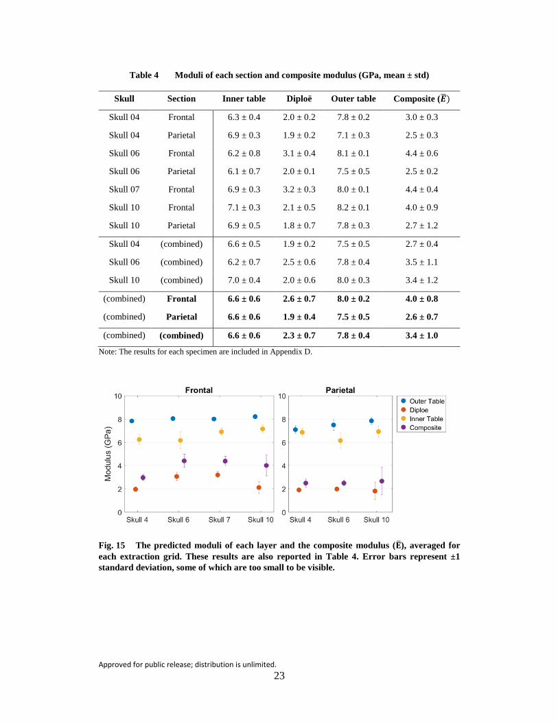
Fig. 15 The predicted moduli of each layer and the composite modulus (E), averaged for each extraction grid. These results are also reported in Table 4. Error bars represent ±1 standard deviation, some of which are too small to be visible. ........................................................................ 23
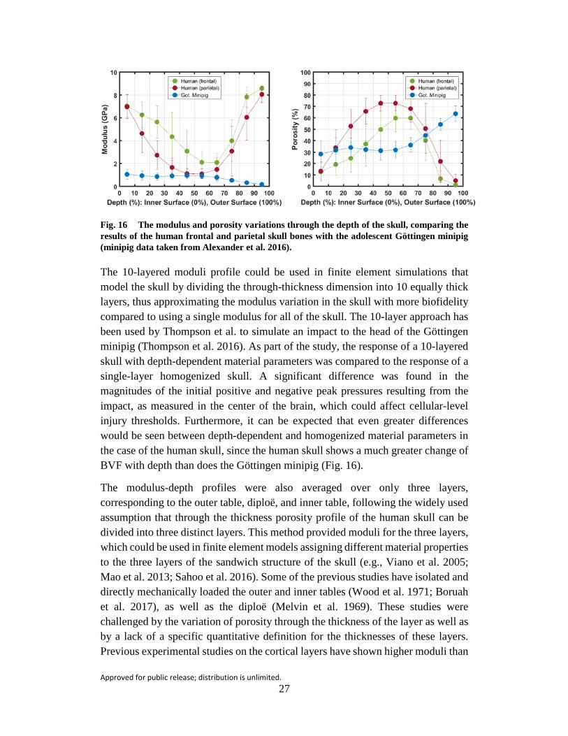
Fig. 16 The modulus and porosity variations through the depth of the skull, comparing the results of the human frontal and parietal skull bones with the adolescent Göttingen minipig (minipig data taken from Alexander et al. 2016). ........................................................................ 27
Fig. A-1 Micro-CT image of Specimen 04-02, taken after extraction from the skull without sanding. Image shows the through-thickness dimension: the top of the image is the outer surface of the skull and the bottom of the image is the inner surface of the skull. .......................................... 37
Fig. A-2 Image from the far camera of the assembly of Specimen 04-02, prior to compression. The difference in speckle density between the platens and the assembly is clearly visible. ..................................................... 38
Fig. A-3 The apparent stress–strain response for Specimen 04-02. The apparent stress was calculated by normalizing the force measurement from the load cell of the loading machine by the nominal cross-sectional area of the specimen. The apparent strain was calculated based on the relative displacement of the platens and the uncompressed height of the specimen. Compression of this specimen was extended beyond diploë failure to investigate the large-strain response and failure. ................ 39
Fig. A-4 The apparent stress–strain response for all three unsanded (assembly) specimens. Inset figure shows detail of the elastic region, with the modulus calculated for each specimen. In the inset, the region of each response curve that was considered in calculating the stiffness (or effective modulus of the sandwich structure) is shown by bolded dotted lines. ......................................................................................... 40
Fig. A-5 The apparent mechanical response of the unsanded and sanded specimens ............................................................................................ 42
Fig. B-1 Compliance error for Specimen 04-06 ................................................ 44
Fig. B-2 Compliance error for Specimen 04-07 ................................................ 45
Fig. B-3 Compliance error for Specimen 04-09 ................................................ 45
Fig. C-1 Thickness percentage of the outer table, diploë, and inner table, averaged by bone type as reported in ARL-TR-7962. Differences
Approved for public release; distribution is unlimited. vii
between frontal and parietal bone thicknesses are significant (Alexander et al. 2017). ...................................................................... 48
List of Tables
Table 1 Elastic and failure parameters from the apparent mechanical response of the nonuniform heterogeneous specimens ...................................... 17
Table 2 Failure stress of the outer and inner tables .......................................... 17
Table 3 Moduli and porosity for each of the 10 equally thick layers .............. 22
Table 4 Moduli of each section and composite modulus (GPa, mean ± std) ... 23
Table 5 Summary of mechanical response for the inner table, diploë and outer table (mean ± std) ................................................................................ 24
Table A-1 Apparent mechanical properties of the sanded and unsanded sandwich-structure specimens ............................................................................. 41
Table C-1 Thickness percentage (%) of each layer (mean ± std) ........................ 47
Table D-1 Moduli for specimens from the frontal bone of Skull 04.................... 50
Table D-2 Moduli for specimens from the parietal bone of Skull 04 .................. 50
Table D-3 Moduli for specimens from the frontal bone of Skull 06.................... 51
Table D-4 Moduli for specimens from the parietal bone of Skull 06 .................. 51
Table D-5 Moduli for specimens from the frontal bone of Skull 07.................... 52
Table D-6 Moduli for specimens from the frontal bone of Skull 10.................... 52
Table D-7 Moduli for specimens from the parietal bone of Skull 10 .................. 53

Approved for public release; distribution is unlimited. 1
1. Introduction
During externally applied mechanical insults to the head, such as blast or impact loading, the skull protects the brain from injuries. Design and evaluation of the effectiveness of head protection devices and concepts depend on the ability to understand the mechanical response of cranial bone to these external loads. Mechanical properties obtained from other bones cannot be used to describe the skull a priori because different bones have different micro-structural details affecting the apparent mechanical response of these bones (Morgan and Keaveny 2001, Morgan et al. 2003). For example, cranial bones have a three-layer sandwich structure. The outer layer closest to the skin is referred to as the outer table (identified as OT), while the inner layer closest to the brain is referred to as the inner table (identified as IT). The middle layer is known as the diploë, and will also be referenced in this report as the mid-diploë (MD). The outer and inner tables are made of dense cortical bone (generally less than 30% porosity), while the diploë is highly porous (Alexander et al. 2017). This sandwich structure of the skull is in contrast to long bones, such as those found in the extremities, where the dense cortical bone is found only at the outer most surface nearest to the skin (Sanborn et al. 2015; Weerasooriya et al. 2016).
Cranial bone also differs in the arrangement of its osteons. Osteons are substructural elements found in cortical bone, and are cylindrical arrangements of collagen-reinforced lamellae that contribute to the stiffness of the bone (Mow and Huiskes 2005; Weerasooriya et al. 2016). The long axis of the osteonal cylinders are arranged in the direction of loading in typical load-bearing bones such as the femur. However, the few studies investigating the osteonal arrangement in the skull cortical bone have concluded that cranial osteons do not show similar trends (Dempster 1967; McElhaney et al. 1970; Alexander et al. 2017; Boruah et al. 2017).
Previous studies have directly characterized the mechanical response of human cranial bone through three-point bending (Hubbard 1971; Motherway et al. 2009; Auperrin et al. 2014; Rahmoun 2014), tension (Boruah et al. 2017), shear (Robbins et al. 1969; McElhaney et al. 1970) and compression (Robbins and Wood 1969; McElhaney et al. 1970; Boruah et al. 2013). However, much variability exists in the data, likely due to natural variability in skull microstructure and bone material as well as differences in testing methods and type of loading. For example, researchers have concluded that large standard deviations within their own studies are likely due to structural variations (McElhaney et al. 1970; Motherway et al. 2009). US Army Research Laboratory (ARL) researchers have previously quantified the significant skull-to-skull variation in the thickness of each of the

Approved for public release; distribution is unlimited. 2
three layers (boundaries defined by the 30% porosity threshold) of the sandwich structure (Alexander et al. 2017). With regard to test methods, Keaveny et al. has shown that calculating the modulus of trabecular bone using the test machine motion can yield results that range between 10% and 260% of the true modulus due to a number of testing artifacts (Keaveny et al. 1993).
The microstructurally based mechanical properties for porcine cranial bone have been previously reported for two different miniature porcine breeds, the Göttingen and Yucatan (Alexander et al. 2016; Gunnarsson et al. 2018). To avoid potential artifacts, strain data from the quasi-static compression tests were measured directly on the specimen using digital image correlation (DIC). The change of modulus through the thickness of the specimen, which depends on the local porosity, was calculated from local strain obtained from the DIC measurements. After observing banding of strain distribution with depth during mechanical compression, Alexander et al. (2016) proposed a layered porous structure for skull bone as a function of depth. The morphology of the bone was measured with high-resolution microcomputed tomography (micro-CT). Both the measured moduli and morphological data showed a large gradient from the inner (brain) to the outer (skin) surfaces of the bone. Power-law relationships had been previously used to relate the far-field modulus of bone to its density or other correlative measures of the bone volume fraction (Helgason et al. 2008). A power-law relationship was used to relate the localized moduli to the localized bone volume fraction in the animal cranial bone, in order to account for the observed gradient in the measured moduli and corresponding morphologies. These depth-dependent modulus relationships were then directly implemented into a computational model of the porcine skull (Thompson et al. 2016). The simulation results showed that implementing depth-dependent mechanical properties for the skull during impact loading significantly influenced the peak pressure predicted in the brain.
The detailed morphological variations of human cranial bone were measured using a high-resolution micro-CT, and have been previously reported (Alexander et al. 2017). The change of porosity as a function of depth was measured, and the variation between the frontal and parietal bones, as well as between different donors, was quantified to identify the intra- and inter-skull variability. Additionally, a method was developed to quantitatively identify the boundaries of the three layers of the skull (outer table, diploë, and inner table) using the porosity-depth profile. Using a quantitative technique to define the layer boundaries was an improvement compared to the majority of previous literature (e.g., McElhaney et al. 1970; Hubbard et al. 1971; Peterson and Dechow 2002, 2003), which qualitatively defined the layer boundaries using visual inspection.
Approved for public release; distribution is unlimited. 3
Here, the morphology of the human skull was related to its mechanical response by further extending the techniques previously reported for the animal skull (Alexander et al. 2016). Several human skull specimens from the previous morphological study (Alexander et al. 2017) were mechanically loaded in quasi-static compression. Two cameras were used to capture the resulting deformation on two adjacent speckled specimen faces. DIC was used to measure the full-field specimen surface strain distribution during deformation. Specimens were assumed to consist of layers acting in series as described by Alexander et al. (2016). Initial elastic moduli of each layer were calculated using a constant uniaxial stress assumption within the specimen and the measured average strain within layers. A power relationship was used to represent the local bone volume fraction (BVF) and the local modulus. The relationship was used to predict the porosity-dependent moduli of all specimens using the measured porosity distributions, as well as the solid bone modulus of the skull bone material. The moduli were averaged over 10 equally thick layers and are included in this report, along with the average moduli for each of the three layers of the sandwich structure (outer table, diploë, and inner table).
2. Methods
2.1 Specimen Extraction and Preparation
Bone specimens were extracted from the skull of a postmortem human subject (PMHS). These specimens were used from a previous study on skull morphology, which fully detailed the donor information and extraction methodology (Alexander et al. 2017). All testing was done in accordance with ARL’s Policy for Use of Human Cadavers for Research, Development, Test, and Evaluation under the guidance and oversight of the ARL Human Cadaver Review Board and the ARL Safety Office. The skull did not have a history of musculoskeletal diseases nor did it demonstrate any macroscopic pathological changes near the specimen extraction sites. In this report, specimen labeling will follow the previously established convention, with precise in-situ locations on the skull having been already documented (Alexander et al. 2017). The specimens originated from the frontal bone of Skull 04 (79 years old). The dimensions on the outer surface were approximately 8 × 8 mm, and the specimens included the entire skull thickness. All specimens were stored in individual vials filled with Hank’s Buffered Saline Solution (HBSS) at 4 °C.
Approved for public release; distribution is unlimited. 4
2.1.1 Composite Specimens
Three specimens were wet-sanded so that the outer and inner surfaces were flat and parallel for compression loading. Sandpaper (180 grit) and a custom lapping device were used for wet-sanding. These specimens will be hereafter referred to as composite specimens, since they consisted of the outer and inner tables as well as the diploë. The labels of the composite specimens, according to previous convention (Alexander et al. 2017), were 04-06, 04-07, and 04-09. Their precise in-situ location relative to the skull sutures was also previously documented (Alexander et al. 2017).
2.1.2 Table Specimens
Table specimens, consisting only of the outer or inner table, were prepared from five other specimens to estimate the compressive failure strengths of the tables: 04-01, 04-02, 04-03, 04-04, and 04-08. Four of these specimens, 04-01, 04-02, 04-03, and 04-04, were first compressed in preliminary experiments using epoxy endcaps (Appendix A), which caused the diploë to fail very early with almost no strain in the table sections of the specimen. Afterwards, the diploë of each of these specimens was cut through to separate the outer half of the specimen from the inner half. Specimen 04-08 was cut through the diploë into two halves with a razor blade prior to any experimentation. For all of the specimens, each half was then wet-sanded to remove the diploë, as determined by visual examination, leaving only the inner and outer table as two separate specimens. Thus, each of the five specimens yielded an outer table specimen and an inner table specimen. These 10 table specimens will be referred to using the previous convention with the suffix OT or IT.
2.2 Morphological Characterization
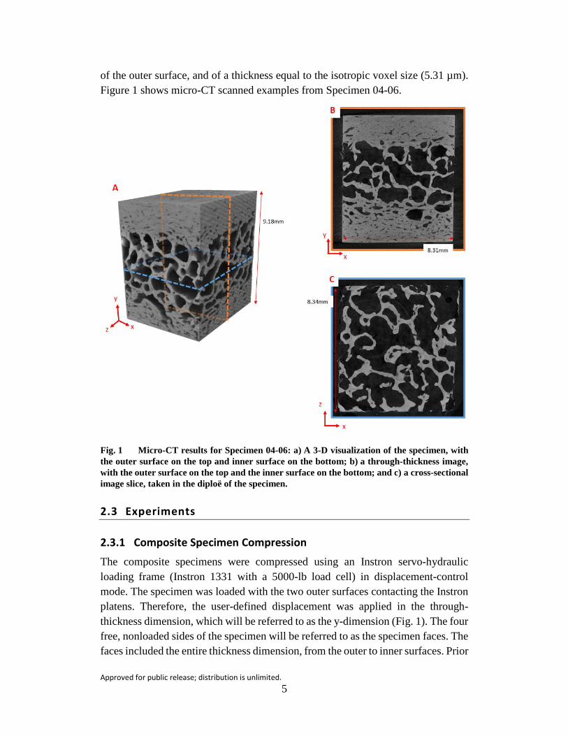
After sanding, the composite and table specimens were imaged using a desktop micro-CT scanner (Skyscan 1172, Bruker microCT, Belgium). The following scan settings were used: 62 kV, 161 µA, 0.15° rotation step, and 10 images averaged for each acquired image. The isotropic voxel size was 5.31 µm. The specimens were wrapped in HBSS-soaked gauze and placed in a radio-translucent tube to keep them hydrated during micro-CT scanning. Image postprocessing followed the same procedures as previously described for the unsanded specimens (Alexander et al. 2017). As a result, each specimen was represented digitally as a stack (series) of roughly 1000 images separated along the depth dimension by a thickness equal to the isotropic voxel size (5.31 µm). The stack of images was oriented such that the normal to the outer table surface was aligned to the loading direction. Each image in the stack represented a cross-sectional slice (Fig. 1c), perpendicular to the normal
Approved for public release; distribution is unlimited. 5
of the outer surface, and of a thickness equal to the isotropic voxel size (5.31 µm). Figure 1 shows micro-CT scanned examples from Specimen 04-06.
Fig. 1 Micro-CT results for Specimen 04-06: a) A 3-D visualization of the specimen, with the outer surface on the top and inner surface on the bottom; b) a through-thickness image, with the outer surface on the top and the inner surface on the bottom; and c) a cross-sectional image slice, taken in the diploë of the specimen.
2.3 Experiments
2.3.1 Composite Specimen Compression
The composite specimens were compressed using an Instron servo-hydraulic loading frame (Instron 1331 with a 5000-lb load cell) in displacement-control mode. The specimen was loaded with the two outer surfaces contacting the Instron platens. Therefore, the user-defined displacement was applied in the through-thickness dimension, which will be referred to as the y-dimension (Fig. 1). The four free, nonloaded sides of the specimen will be referred to as the specimen faces. The faces included the entire thickness dimension, from the outer to inner surfaces. Prior

Approved for public release; distribution is unlimited. 6
to loading the specimens, two adjacent faces (joined by a single edge) were spray painted to apply speckle patterns necessary for DIC measurement of displacements. The compression platens of the Instron loading frame were also speckled to enable DIC tracking of the relative movement between the two platens, which were directly in contact with the specimen. DIC tracking of the platen movement provided a more accurate determination of the global specimen strain than the machine displacement, which includes the machine compliance, as shown in Appendix B.
Two cameras (Point Grey Research Grasshopper; 12.3 megapixels; resolution = 2824 × 4240) were used to capture the deformation of the two adjacent speckled faces during deformation. As shown in Fig. 2, one camera was focused on the left face (referred to as the left camera), and the other camera was focused on the right face (referred to as the right camera). The field of view of the cameras included part of the speckle patterns on the loading platens (Figs. 2b and 2c). The images of the speckle patterns were postprocessed using VIC-2D (Correlated Solutions Inc.) to calculate displacement and strain fields. The subset size used for correlations varied across specimens and was based on speckling and image quality: 55 pixels for both cameras of Specimens 04-06 and 04-07, and 45 pixels for both cameras of Specimen 04-09.
Machine displacement was specified to achieve a nominal strain rate of 0.001/s, with load and displacement data recorded during loading. The experiments were stopped when macroscopic damage of the specimen surface obscured the speckle pattern (Section 3.2).

Approved for public release; distribution is unlimited. 7
Fig. 2 Experimental setup: a) Instron loading frame with two cameras and specimen prior to compression (detail shown in inset). Typical camera images are shown in b) and c), both from Specimen 04-06.
2.3.2 Table Specimen Compression
The table specimens were loaded in order to obtain their compressive failure strength. The same load frame, displacement rate, and cameras were used as for the composite specimens. Experiments were stopped after macroscopic failure of the specimens was visually identified.
Approved for public release; distribution is unlimited. 8
3. Results
3.1 Porosity Variation
3.1.1 Porosity-Depth Profiles
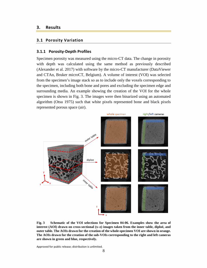
Specimen porosity was measured using the micro-CT data. The change in porosity with depth was calculated using the same method as previously described (Alexander et al. 2017) with software by the micro-CT manufacturer (DataViewer and CTAn, Bruker microCT, Belgium). A volume of interest (VOI) was selected from the specimen’s image stack so as to include only the voxels corresponding to the specimen, including both bone and pores and excluding the specimen edge and surrounding media. An example showing the creation of the VOI for the whole specimen is shown in Fig. 3. The images were then binarized using an automated algorithm (Otsu 1975) such that white pixels represented bone and black pixels represented porous space (air).
Fig. 3 Schematic of the VOI selections for Specimen 04-06. Examples show the area of interest (AOI) drawn on cross-sectional (x–z) images taken from the inner table, diploë, and outer table. The AOIs drawn for the creation of the whole-specimen VOI are shown in orange. The AOIs drawn for the creation of the sub-VOIs corresponding to the right and left cameras are shown in green and blue, respectively.

Approved for public release; distribution is unlimited. 9
After rotation of the specimen was applied during postprocessing (Section 2.2), the image stack was aligned to the thickness dimension of the specimen. Each image within the stack was normal to the axis connecting the outer surface to the inner surface. The average porosity, 𝑃𝑃𝑖𝑖, was calculated for each cross-sectional image as the ratio of black pixels to total number of pixels within the VOI.
Therefore, the porosity of each image was assigned as the porosity at the image depth along the image stack at 𝑑𝑑𝑖𝑖, 𝑃𝑃(𝑑𝑑𝑖𝑖) = 𝑃𝑃𝑖𝑖. This procedure for all images produced the porosity-depth profile of the specimen, 𝑃𝑃(𝑑𝑑). The depth of the specimen was then normalized, so that specimens of differing total thickness (depth) can be directly compared. The porosity-depth profile determined by this method represented an average over the entire specimen cross section (x–z plane in Fig. 1).
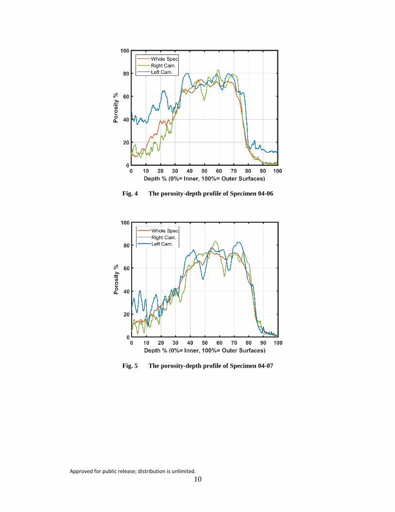
For the composite specimens (IT-MD-OT), localized porosity-depth profiles were also calculated for the region of the specimen nearest to each of the cameras (left-right). First, the position of the cameras was noted relative to prominent specimen features that were visually identifiable by the unaided eye. These features were then located in the 3-D visualization of the micro-CT dataset using the software DataViewer, which also allowed identification of several smaller microscopic features. Finally, the macroscopic and microscopic features were also located within the individual image slices in order to identify the sides of the image slices corresponding with the left and right cameras. After left-right identification, sub-VOIs were created to represent the portion of the specimen nearest to each of the cameras. Each sub-VOI occupied between 9% and 19% of the area of the entire cross-sectional image. Figure 3 shows an example of the creation of sub-VOIs for the two cameras. The VOIs were then binarized and the porosity within the VOI was calculated using the same procedure as above. Figures 4–6 show the resulting porosity-depth profiles for Specimens 04-06, 04-07, and 04-09.
Approved for public release; distribution is unlimited. 10
Fig. 4 The porosity-depth profile of Specimen 04-06
Fig. 5 The porosity-depth profile of Specimen 04-07

Approved for public release; distribution is unlimited. 11
Fig. 6 The porosity-depth profile of Specimen 04-09
Figure 7 shows the 𝑃𝑃(𝑑𝑑) profiles of the table specimens overlaid on the 𝑃𝑃(𝑑𝑑) profile of the original specimens from which they were isolated. The 𝑃𝑃(𝑑𝑑) profiles of the source specimens had been obtained in the previous study (Alexander et al. 2017). The positions of the 𝑃𝑃(𝑑𝑑) profiles of the table specimens along the depth dimension were determined by minimizing the least squares error between the 𝑃𝑃(𝑑𝑑) profiles of the original composite specimens and the table specimens.

Approved for public release; distribution is unlimited. 12
Fig. 7 The porosity-depth profiles of the table specimens compared with the profile of the original (whole) specimen from which they originated
3.1.2 Layer Thickness
The thickness of the outer table, diploë, and inner table were calculated from the porosity-depth profile of each specimen following a previously presented method (Alexander et al. 2017). The method approximated the outer and inner tables as cortical bone and the diploë as trabecular bone. As mentioned in the previous report, it assumed that cortical bone is generally considered to have a porosity of less than 30%, while trabecular bone has a porosity of greater than 30% (Mow et al. 2005).
The method to find the transition points between layers started at the outer surface, where 𝑑𝑑 = 100%. At the outer surface, the cross-sectional porosity was always less than 30% (𝑃𝑃𝑑𝑑=100% < 30%, using the notation of P presented in Section 3.1.1). The method then iteratively checked each lower depth until the depth at which the porosity first exceeded 30% was found. This depth, 𝑑𝑑𝑂𝑂𝑂𝑂→𝑀𝑀𝑀𝑀, was taken as the transition point between the OT and the MD. The depth was then further decreased until the first time that the porosity was again less than 30%. The corresponding depth, 𝑑𝑑𝑀𝑀𝑀𝑀→𝐼𝐼𝑂𝑂, was noted as the transition point between the IT and the MD. Using the notation of Section 3.1.1, this process is summarized as follows:
Approved for public release; distribution is unlimited. 13
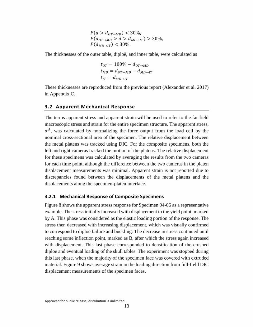
𝑃𝑃(𝑑𝑑 > 𝑑𝑑𝑂𝑂𝑂𝑂→𝑀𝑀𝑀𝑀) < 30%, 𝑃𝑃(𝑑𝑑𝑂𝑂𝑂𝑂→𝑀𝑀𝑀𝑀 > 𝑑𝑑 > 𝑑𝑑𝑀𝑀𝑀𝑀→𝐼𝐼𝑂𝑂) > 30%, 𝑃𝑃(𝑑𝑑𝑀𝑀𝑀𝑀→𝐼𝐼𝑂𝑂) < 30%.
The thicknesses of the outer table, diploë, and inner table, were calculated as
𝑡𝑡𝑂𝑂𝑂𝑂 = 100% − 𝑑𝑑𝑂𝑂𝑂𝑂→𝑀𝑀𝑀𝑀 𝑡𝑡𝑀𝑀𝑀𝑀 = 𝑑𝑑𝑂𝑂𝑂𝑂→𝑀𝑀𝑀𝑀 − 𝑑𝑑𝑀𝑀𝑀𝑀→𝐼𝐼𝑂𝑂 𝑡𝑡𝐼𝐼𝑂𝑂 = 𝑑𝑑𝑀𝑀𝑀𝑀→𝐼𝐼𝑂𝑂
These thicknesses are reproduced from the previous report (Alexander et al. 2017) in Appendix C.
3.2 Apparent Mechanical Response
The terms apparent stress and apparent strain will be used to refer to the far-field macroscopic stress and strain for the entire specimen structure. The apparent stress, 𝜎𝜎𝐴𝐴, was calculated by normalizing the force output from the load cell by the nominal cross-sectional area of the specimen. The relative displacement between the metal platens was tracked using DIC. For the composite specimens, both the left and right cameras tracked the motion of the platens. The relative displacement for these specimens was calculated by averaging the results from the two cameras for each time point, although the difference between the two cameras in the platen displacement measurements was minimal. Apparent strain is not reported due to discrepancies found between the displacements of the metal platens and the displacements along the specimen-platen interface.
3.2.1 Mechanical Response of Composite Specimens
Figure 8 shows the apparent stress response for Specimen 04-06 as a representative example. The stress initially increased with displacement to the yield point, marked by A. This phase was considered as the elastic loading portion of the response. The stress then decreased with increasing displacement, which was visually confirmed to correspond to diploë failure and buckling. The decrease in stress continued until reaching some inflection point, marked as B, after which the stress again increased with displacement. This last phase corresponded to densification of the crushed diploë and eventual loading of the skull tables. The experiment was stopped during this last phase, when the majority of the specimen face was covered with extruded material. Figure 9 shows average strain in the loading direction from full-field DIC displacement measurements of the specimen faces.

Approved for public release; distribution is unlimited. 14
Fig. 8 A representative example of the apparent average stress response (load/area) for the human skull specimens, taken from the results for Specimen 04-06. Point A corresponds to a yield point, point B corresponds to the inflection point after which stress again increases with displacement, and point C is taken during the reloading portion.

Approved for public release; distribution is unlimited. 15
Fig. 9 DIC results for the specimen faces. Contours are of the surface strain in the compression direction (𝜺𝜺𝒚𝒚𝒚𝒚𝑨𝑨 ) for Specimen 04-06 at the yield point (A), inflection point (B), and during the reloading phase (C). The letters A, B, and C correspond with the markings of Fig. 8. The specimen height (distance between platens) at each point was: 9.39 mm at A, 8.89 mm at B, and 6.93 mm at C.
Figure 10 shows the apparent mechanical response for the three specimens 04-06, 04-07, and 04-09; each were nonuniform structures with varying microstructures. The apparent stiffness during the initial loading phase was calculated for each

Approved for public release; distribution is unlimited. 16
specimen. First, the displacement applied during the experiment was normalized by the original distance between platens. A linear regression was then fit to the initial portion of the loading curve.
Fig. 10 The apparent average stress (load/area) as a function of displacement of the composite specimens
The failure stress was calculated in three ways. For all three techniques, the failure stress used the load peak just prior to diploë collapse and fracture softening. The three techniques differed in the cross-sectional area (CSA) used to calculate the failure stress. The first technique used apparent specimen CSA obtained with calipers. This method did not account for the reduced CSA in the specimen due to porosity.
The other two methods accounted for the reduced specimen CSA in the diploë region by normalizing the area by the BVF ratio in the diploë. Accounting for the reduced BVF provided a more accurate CSA to use in calculating failure stress for bone tissue, as the failure stress after elastic loading was driven by collapse and fracture of trabeculae in the diploë. The second method used the average BVF over the entire diploë region, while the third method used the diploë minimum BVF, therefore providing the smallest CSA and largest failure strength. Table 1 lists the apparent stiffnesses and failure stresses.
Approved for public release; distribution is unlimited. 17
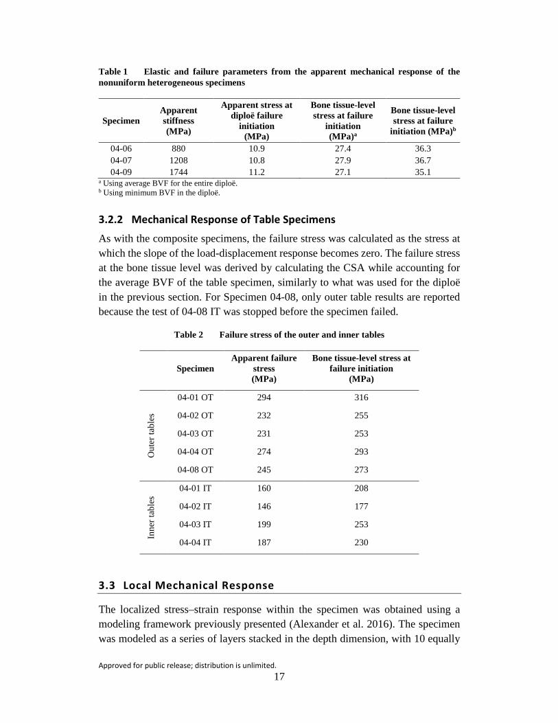
Table 1 Elastic and failure parameters from the apparent mechanical response of the nonuniform heterogeneous specimens
Specimen Apparent stiffness (MPa)
Apparent stress at diploë failure
initiation (MPa)
Bone tissue-level stress at failure
initiation (MPa)a
Bone tissue-level stress at failure
initiation (MPa)b
04-06 880 10.9 27.4 36.3 04-07 1208 10.8 27.9 36.7 04-09 1744 11.2 27.1 35.1
a Using average BVF for the entire diploë. b Using minimum BVF in the diploë.
3.2.2 Mechanical Response of Table Specimens
As with the composite specimens, the failure stress was calculated as the stress at which the slope of the load-displacement response becomes zero. The failure stress at the bone tissue level was derived by calculating the CSA while accounting for the average BVF of the table specimen, similarly to what was used for the diploë in the previous section. For Specimen 04-08, only outer table results are reported because the test of 04-08 IT was stopped before the specimen failed.
Table 2 Failure stress of the outer and inner tables
Specimen Apparent failure
stress (MPa)
Bone tissue-level stress at failure initiation
(MPa)
Out
er ta
bles
04-01 OT 294 316
04-02 OT 232 255
04-03 OT 231 253
04-04 OT 274 293
04-08 OT 245 273
Inne
r tab
les
04-01 IT 160 208
04-02 IT 146 177
04-03 IT 199 253
04-04 IT 187 230
3.3 Local Mechanical Response
The localized stress–strain response within the specimen was obtained using a modeling framework previously presented (Alexander et al. 2016). The specimen was modeled as a series of layers stacked in the depth dimension, with 10 equally
Approved for public release; distribution is unlimited. 18
thick layers between the inner and outer surfaces. Local strain measures of the two adjacent specimen surfaces were obtained using the VIC-2D software (Correlated Solutions) to postprocess the speckle images captured from each camera during mechanical loading. The vertical strain in the loading direction, 𝜀𝜀𝑦𝑦𝑦𝑦, the horizontal strain, 𝜀𝜀𝑥𝑥𝑥𝑥, and the shear strain, 𝜀𝜀𝑥𝑥𝑦𝑦, were calculated over the specimen face as a function of time and location: 𝜀𝜀𝑦𝑦𝑦𝑦(𝑥𝑥,𝑦𝑦, 𝑡𝑡), 𝜀𝜀𝑥𝑥𝑥𝑥(𝑥𝑥, 𝑦𝑦, 𝑡𝑡), and 𝜀𝜀𝑥𝑥𝑦𝑦(𝑥𝑥,𝑦𝑦, 𝑡𝑡). Then, for each layer, 𝑛𝑛, the layer-specific strains, 𝜀𝜀𝑦𝑦𝑦𝑦𝑛𝑛 (𝑡𝑡), 𝜀𝜀𝑥𝑥𝑥𝑥𝑛𝑛 (𝑡𝑡), and 𝜀𝜀𝑥𝑥𝑦𝑦𝑛𝑛 (𝑡𝑡) were calculated by averaging the strain data located within the x-y area of each layer.
The stress of each layer, 𝜎𝜎𝑛𝑛, was assumed to be the same as the apparent stress calculated from the load cell, 𝜎𝜎𝑛𝑛 = 𝜎𝜎𝐴𝐴 (this assumption is analyzed in Section 4). The compressive stress–strain response of the layer was then plotted using 𝜎𝜎𝑛𝑛 and 𝜀𝜀𝑦𝑦𝑦𝑦𝑛𝑛 . Finally, the localized modulus of each layer, 𝐸𝐸𝑛𝑛, was calculated from a linear fit to the initial portion of the stress–strain curve for that layer.
3.4 Relating Morphology and Mechanics
3.4.1 Modulus-BVF Power Relationship
The bone volume fraction (BVF or 𝑓𝑓𝐵𝐵𝐵𝐵) of each image is defined as the number of pixels corresponding to the bone as a fraction of the total number of pixels in the image. Therefore, the BVF can be calculated by subtracting the porosity fraction from 1. The BVF-depth profile, 𝑓𝑓𝐵𝐵𝐵𝐵(𝑑𝑑) was obtained as
𝑓𝑓𝐵𝐵𝐵𝐵(𝑑𝑑) = 1 − 𝑃𝑃(𝑑𝑑). (1)
The average bone volume fraction of each layer was then calculated by averaging 𝑓𝑓𝐵𝐵𝐵𝐵(𝑑𝑑) over the depth of the layer.
Figure 11 plots the modulus of each layer (𝐸𝐸𝑛𝑛, Section 3.3) as a function of its average BVF. A power relationship was used to represent the layer modulus and the layer BVF, 𝐸𝐸 = 𝐸𝐸0(𝑓𝑓𝐵𝐵𝐵𝐵)𝑘𝑘 , where 𝑘𝑘 exponentially scales the effect of the BVF and 𝐸𝐸0 corresponds to the modulus of pure bone (100% dense bone). Pure bone material, or tissue, is defined as the completely solid portion of the specimen, with zero porosity (𝑓𝑓𝐵𝐵𝐵𝐵=1). In modulus units of GPa, the power law that was obtained minimizing the sum of squares of errors is given by
𝐸𝐸 = 8.755(𝑓𝑓𝑏𝑏𝑏𝑏) 1.603
. (2)

Approved for public release; distribution is unlimited. 19
Fig. 11 The modulus of each layer (𝑬𝑬𝒏𝒏) plotted as a function of the layer’s BVF. The resulting power relationship between modulus and BVF is shown together with the 95% confidence interval.
3.4.2 Predicted Modulus-Depth Profiles for All Specimens
The change of modulus as a function of depth through the specimens was predicted by applying Eq. 2 to the depth-variation of BVF, 𝑓𝑓𝐵𝐵𝐵𝐵(𝑑𝑑). The porosity-depth profiles were extracted from the micro-CT data of the 63 specimens reported previously (Alexander et al. 2017). The BVF profile of each specimen, 𝑓𝑓𝐵𝐵𝐵𝐵(𝑑𝑑), was then calculated using Eq. 1. Figure 12 provides an example of 𝑃𝑃(𝑑𝑑) and 𝐸𝐸(𝑑𝑑) for Specimen 04-01.
Approved for public release; distribution is unlimited. 20
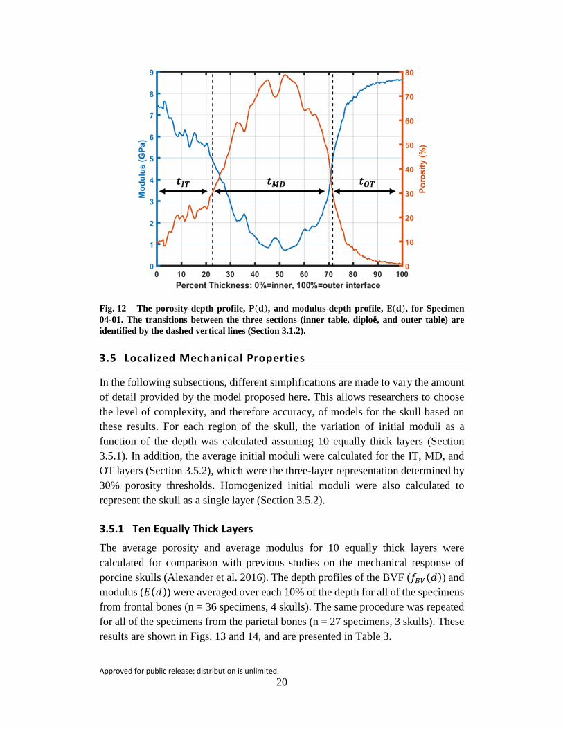
Fig. 12 The porosity-depth profile, 𝐏𝐏(𝐝𝐝), and modulus-depth profile, 𝐄𝐄(𝐝𝐝), for Specimen 04-01. The transitions between the three sections (inner table, diploë, and outer table) are identified by the dashed vertical lines (Section 3.1.2).
3.5 Localized Mechanical Properties
In the following subsections, different simplifications are made to vary the amount of detail provided by the model proposed here. This allows researchers to choose the level of complexity, and therefore accuracy, of models for the skull based on these results. For each region of the skull, the variation of initial moduli as a function of the depth was calculated assuming 10 equally thick layers (Section 3.5.1). In addition, the average initial moduli were calculated for the IT, MD, and OT layers (Section 3.5.2), which were the three-layer representation determined by 30% porosity thresholds. Homogenized initial moduli were also calculated to represent the skull as a single layer (Section 3.5.2).
3.5.1 Ten Equally Thick Layers
The average porosity and average modulus for 10 equally thick layers were calculated for comparison with previous studies on the mechanical response of porcine skulls (Alexander et al. 2016). The depth profiles of the BVF (𝑓𝑓𝐵𝐵𝐵𝐵(𝑑𝑑)) and modulus (𝐸𝐸(𝑑𝑑)) were averaged over each 10% of the depth for all of the specimens from frontal bones (n = 36 specimens, 4 skulls). The same procedure was repeated for all of the specimens from the parietal bones (n = 27 specimens, 3 skulls). These results are shown in Figs. 13 and 14, and are presented in Table 3.
Approved for public release; distribution is unlimited. 21
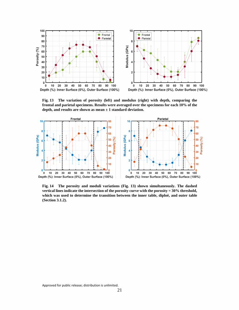
Fig. 13 The variation of porosity (left) and modulus (right) with depth, comparing the frontal and parietal specimens. Results were averaged over the specimens for each 10% of the depth, and results are shown as mean ± 1 standard deviation.
Fig. 14 The porosity and moduli variations (Fig. 13) shown simultaneously. The dashed vertical lines indicate the intersection of the porosity curve with the porosity = 30% threshold, which was used to determine the transition between the inner table, diploë, and outer table (Section 3.1.2).
Approved for public release; distribution is unlimited. 22
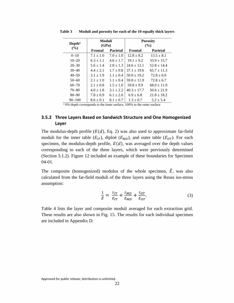
Table 3 Moduli and porosity for each of the 10 equally thick layers
Deptha
(%)
Moduli (GPa)
Porosity (%)
Frontal Parietal Frontal Parietal 0–10 7.1 ± 1.0 7.0 ± 1.0 12.8 ± 8.2 13.5 ± 8.1
10–20 6.3 ± 1.1 4.6 ± 1.7 19.1 ± 9.2 33.9 ± 15.7 20–30 5.6 ± 1.4 2.8 ± 1.3 24.6 ± 12.1 52.8 ± 14.4 30–40 4.4 ± 2.1 1.7 ± 0.8 37.1 ± 19.6 65.7 ± 11.3 40–50 3.1 ± 1.9 1.1 ± 0.4 50.0 ± 19.2 72.8 ± 6.9 50–60 2.1 ± 1.0 1.1 ± 0.4 59.8 ± 11.9 72.8 ± 6.7 60–70 2.1 ± 0.8 1.5 ± 1.0 59.8 ± 9.9 68.0 ± 11.9 70–80 4.0 ± 1.8 3.1 ± 2.2 40.3 ± 17.7 50.6 ± 21.9 80–90 7.8 ± 0.9 6.1 ± 2.0 6.9 ± 6.8 21.8 ± 18.2
90–100 8.6 ± 0.1 8.1 ± 0.7 1.3 ± 0.7 5.2 ± 5.4 a 0% depth corresponds to the inner surface, 100% to the outer surface
3.5.2 Three Layers Based on Sandwich Structure and One Homogenized Layer
The modulus-depth profile (𝐸𝐸(𝑑𝑑), Eq. 2) was also used to approximate far-field moduli for the inner table (𝐸𝐸𝐼𝐼𝑂𝑂), diploë (𝐸𝐸𝑀𝑀𝑀𝑀), and outer table (𝐸𝐸𝑂𝑂𝑂𝑂). For each specimen, the modulus-depth profile, 𝐸𝐸(𝑑𝑑), was averaged over the depth values corresponding to each of the three layers, which were previously determined (Section 3.1.2). Figure 12 included an example of these boundaries for Specimen 04-01.
The composite (homogenized) modulus of the whole specimen, 𝐸𝐸�, was also calculated from the far-field moduli of the three layers using the Reuss iso-stress assumption:
1𝐸𝐸�
= 𝑡𝑡𝐼𝐼𝐼𝐼𝐸𝐸𝐼𝐼𝐼𝐼
+ 𝑡𝑡𝑀𝑀𝑀𝑀𝐸𝐸𝑀𝑀𝑀𝑀
+ 𝑡𝑡𝑂𝑂𝐼𝐼𝐸𝐸𝑂𝑂𝐼𝐼
. (3)
Table 4 lists the layer and composite moduli averaged for each extraction grid. These results are also shown in Fig. 15. The results for each individual specimen are included in Appendix D.
Approved for public release; distribution is unlimited. 23
Table 4 Moduli of each section and composite modulus (GPa, mean ± std)
Skull Section Inner table Diploë Outer table Composite (𝑬𝑬�)
Skull 04 Frontal 6.3 ± 0.4 2.0 ± 0.2 7.8 ± 0.2 3.0 ± 0.3
Skull 04 Parietal 6.9 ± 0.3 1.9 ± 0.2 7.1 ± 0.3 2.5 ± 0.3
Skull 06 Frontal 6.2 ± 0.8 3.1 ± 0.4 8.1 ± 0.1 4.4 ± 0.6
Skull 06 Parietal 6.1 ± 0.7 2.0 ± 0.1 7.5 ± 0.5 2.5 ± 0.2
Skull 07 Frontal 6.9 ± 0.3 3.2 ± 0.3 8.0 ± 0.1 4.4 ± 0.4
Skull 10 Frontal 7.1 ± 0.3 2.1 ± 0.5 8.2 ± 0.1 4.0 ± 0.9
Skull 10 Parietal 6.9 ± 0.5 1.8 ± 0.7 7.8 ± 0.3 2.7 ± 1.2
Skull 04 (combined) 6.6 ± 0.5 1.9 ± 0.2 7.5 ± 0.5 2.7 ± 0.4
Skull 06 (combined) 6.2 ± 0.7 2.5 ± 0.6 7.8 ± 0.4 3.5 ± 1.1
Skull 10 (combined) 7.0 ± 0.4 2.0 ± 0.6 8.0 ± 0.3 3.4 ± 1.2
(combined) Frontal 6.6 ± 0.6 2.6 ± 0.7 8.0 ± 0.2 4.0 ± 0.8
(combined) Parietal 6.6 ± 0.6 1.9 ± 0.4 7.5 ± 0.5 2.6 ± 0.7
(combined) (combined) 6.6 ± 0.6 2.3 ± 0.7 7.8 ± 0.4 3.4 ± 1.0
Note: The results for each specimen are included in Appendix D.
Fig. 15 The predicted moduli of each layer and the composite modulus (𝐄𝐄�), averaged for each extraction grid. These results are also reported in Table 4. Error bars represent ±1 standard deviation, some of which are too small to be visible.

Approved for public release; distribution is unlimited. 24
3.5.3 Summary of Mechanical Response of the Inner Table, Diploë, and Outer Table
Table 5 presents a summary for the modulus and failure stress of the inner table, diploë, and outer table. The data was taken from the results of direct experimentation of the composite specimens (Section 3.2.1) and table specimens (Section 3.2.2), together with the modeling results (Section 3.5.2).
Table 5 Summary of mechanical response for the inner table, diploë and outer table (mean ± std)
Inner table Diploë Outer table Composite
Modulus (GPa) 6.6 ± 0.6a 2.3 ± 0.7a 7.8 ± 0.4a 3.4 ± 1.0a
Failure strength (MPa) 173 ± 24b 11.0 ± 0.2c 255 ± 28b 11.0 ± 0.2c a From results of the E-BVF model and morphology (Section 3.5.2)
b From experimental results of the table specimens (Section 3.2.2)
c From experimental results of the composite specimens (Section 3.2.1)
4. Discussion
4.1 Apparent Structural Response of the Composite Specimens
The composite heterogeneous skull specimens were mechanically compressed as complete structures. The apparent stress–strain response was obtained using force measurements from the load cell of the testing machine and far-field displacement measurements from DIC of the speckled platens. The stiffness calculated from the slope of the initial linear portion of the apparent stress–strain response therefore represents the structural modulus of the entire thickness of the specimen, and the results ranged between 0.9 and 1.7 GPa. The few previous studies, where the entire structure was loaded in compression, do not present a conclusive range of values for the apparent modulus or stiffness. For example, the present stiffness numbers are similar to the ranges of stiffnesses reported by Robbins et al. (0.7–3.6 GPa) and McElhaney et al. (2.4 ± 1.4 GPa) (Robbins et al. 1969; McElhaney et al. 1970). In contrast, Boruah et al. reported lower stiffness values of 0.5 ± 0.1 GPa (Boruah et al. 2013). Considerations for inter-study comparisons are further discussed in Section 4.3.
The apparent stress–strain response of the human skull specimens exhibited approximately three different phases during uniaxial compression: initial loading, diploë buckling and failure, and further reloading. The first phase was the initial loading of the complete structure. This phase included an initial random “toe”
Approved for public release; distribution is unlimited. 25
region, which likely arose from contact between the platens and any surface artifacts or roughness on the outer and inner surfaces of the specimens, as others have also observed (Boruah et al. 2013). After the “toe” region, the stress increased almost linearly with deformation until the yield point.
The yield point likely corresponded with the beginning of trabeculae failure inside the diploë, as others have also concluded (Boruah et al. 2013; Robbins et al. 1969). This conclusion was supported by the observation that material was ejected from the middle portion of the specimen as it was loaded beyond the yield point. Moreover, at the “yield”, DIC started to break down in the diploë region due to strain localization accompanied with pockets of concentrated large deformation zones, as seen in Fig. 9a. Examples of ejections could be seen in the images of Fig. 9 taken after the yield point (Figs. 9b and 9c). Furthermore, the outer and inner tables appeared intact even after the final loading was completed, further showing that failure occurred within the diploë. This is to be expected, as the tables are denser than the diploë.
Since yield was associated with failure in the diploë, the failure stress of the composite specimens at the bone tissue level was approximated by accounting for the porosity of the diploë (last two columns of Table 1). Similarly, the bone-tissue-level failure stress within the table specimens was derived by accounting for their average porosity (last column of Table 2). The goal was to compare these bone-tissue-level failure stresses within the composite and table specimens. However, the failure stresses of the composite specimens were still an order of magnitude less than those for the table specimens, even after normalizing the CSA by the peak values of porosity within the diploë. This result is likely due to the fact that the bone material within the diploë is not vertically aligned in the loading direction, but is instead arranged at various angles from vertical. The dissimilarity in failure stresses underlines the influence of the microstructural arrangement of the bone within the diploë on the mechanical properties.
All three specimens exhibited a decrease in stress after the yield point, prior to the reloading phase. The post-yield decrease in stress prior to reloading has not been universally observed in the skull, with some specimens showing only a stress plateau or simply a kink in the stress–strain response (Robbins et al. 1969; Boruah et al. 2013). However, Robbins et al. reported that the post-yield decrease in stress was the most commonly observed response (Robbins et al. 1969). The variation could be due to variation in the porosity of the diploë. It could also be due to differences in strain measurement method, since test machine compliance affects the final displacement measurement. Cellular materials such as foams and honeycombs have also been shown to exhibit three-phase responses, with variation

Approved for public release; distribution is unlimited. 26
in the overall shape of the stress–strain response arising from the relative density and microstructure (Gibson and Ashby 1997).
The stress–strain response during reloading had a lower slope than the initial loading phase, as also observed in previous studies (Robbins et al. 1969; Boruah et al. 2013). The lower slope of the reloading phase is likely caused by densification of the failed diploë material. However, during further compression, the specimen continued to solidify until the relatively solid table regions started to carry significant load. This caused the slope of the reloading phase to increase with displacement in the densification region (green region of Fig. 8).
4.2 Layered Response
A simplified material model was used to extract depth-dependency of the initial modulus. The power relationship of Eq. 2 related the localized modulus to the localized BVF. The parameter 𝐸𝐸0 = 8.8 GPa corresponds to the modulus for pure bone (BVF = 100%, also referred to as the bone tissue modulus). There have only been a few other studies that have reported the tissue modulus for human cranial bone using modeling techniques, though the results have not been conclusive (e.g., Rahmoun et al. 2014; Boruah et al. 2017). Rahmoun et al. loaded cranial bone in three-point bending and used anisotropic and isotropic models to calculate the tissue modulus as 4.9 or 3.8 GPa, respectively (Rahmoun et al. 2014). On the other hand, Boruah et al. tested the outer table in dynamic tension and reported a tissue modulus of 18.5 GPa (Boruah et al. 2017). The differences could be attributed to the assumptions that are used during different modeling concepts and also to the variations in loading type and experimental procedures.
In this report, the modulus-depth profiles were averaged by three methods. In the first method, the depth dimension was divided into 10 layers of equal thickness and the modulus was averaged over each layer. This method allowed comparison of human skull moduli with previously obtained moduli for the cranial bone of the adolescent Göttingen minipig (Alexander et al. 2016). In that study, the depth dimension was divided into 10 layers of equal thickness due to the observed porosity gradient along the depth of the bone. In contrast to human skull, the average BVF-depth profile of the adolescent minipig skull gradually decreased from the inner surface (72%) to the outer surface (36%). Figure 16 compares the BVF-depth and modulus-depth profiles between the human and the Göttingen minipig.
Approved for public release; distribution is unlimited. 27
Fig. 16 The modulus and porosity variations through the depth of the skull, comparing the results of the human frontal and parietal skull bones with the adolescent Göttingen minipig (minipig data taken from Alexander et al. 2016).
The 10-layered moduli profile could be used in finite element simulations that model the skull by dividing the through-thickness dimension into 10 equally thick layers, thus approximating the modulus variation in the skull with more biofidelity compared to using a single modulus for all of the skull. The 10-layer approach has been used by Thompson et al. to simulate an impact to the head of the Göttingen minipig (Thompson et al. 2016). As part of the study, the response of a 10-layered skull with depth-dependent material parameters was compared to the response of a single-layer homogenized skull. A significant difference was found in the magnitudes of the initial positive and negative peak pressures resulting from the impact, as measured in the center of the brain, which could affect cellular-level injury thresholds. Furthermore, it can be expected that even greater differences would be seen between depth-dependent and homogenized material parameters in the case of the human skull, since the human skull shows a much greater change of BVF with depth than does the Göttingen minipig (Fig. 16).
The modulus-depth profiles were also averaged over only three layers, corresponding to the outer table, diploë, and inner table, following the widely used assumption that through the thickness porosity profile of the human skull can be divided into three distinct layers. This method provided moduli for the three layers, which could be used in finite element models assigning different material properties to the three layers of the sandwich structure of the skull (e.g., Viano et al. 2005; Mao et al. 2013; Sahoo et al. 2016). Some of the previous studies have isolated and directly mechanically loaded the outer and inner tables (Wood et al. 1971; Boruah et al. 2017), as well as the diploë (Melvin et al. 1969). These studies were challenged by the variation of porosity through the thickness of the layer as well as by a lack of a specific quantitative definition for the thicknesses of these layers. Previous experimental studies on the cortical layers have shown higher moduli than
Approved for public release; distribution is unlimited. 28
the results presented here for the outer and inner tables (7.8 ± 0.4 and 6.6 ± 0.6 GPa, respectively). For example, Wood et al. measured the tensile modulus of the outer and inner tables to range from 10.3 to 22.1 GPa, based on increasing the strain rate from 0.005 to 150/s (Wood et al. 1971). Similarly, Boruah et al. measured the modulus of the outer table to be 12.0 ± 3.3 GPa, as tested under dynamically applied tension (Boruah et al. 2017). Some possible reasons for these discrepancies are discussed in Section 4.3. On the other hand, the modulus of the diploë (2.3 ± 0.7 GPa) in this study falls within the 0.4- to 2.8-GPa range reported by Melvin et al. for bones tested by compression (Melvin et al. 1969).
4.3 Limitations, Assumptions and Inter-Study Comparisons
Discrepancies between the present results and previous literature are likely due to different testing techniques in addition to the limitations and assumptions in each study. Material properties obtained from mechanical characterization of bone are highly sensitive to the experimental protocols, as bone is a complex, heterogeneous, multi-scale biomaterial. This especially hinders inter-study comparisons for the case of the human skull because the literature is already sparse. For example, several of the studies mentioned previously were based on either tension tests (e.g., Wood et al. 1971; Boruah et al. 2017) or bending tests, which involve a combination of compression and tension (e.g., Motherway et al. 2009; Rahmoun et al. 2014). However, the mechanical properties of bone in compression and tension are not the same, as has been shown, for example, for ultimate strains and stresses (Keaveny et al. 2004). Furthermore, the modulus of bone has been shown to vary with loading rate (Wood et al. 1971; Sanborn et al. 2015). The few studies that have reported the apparent, far-field compression response of human skull specimens have used differing strain rates (McElhaney et al. 1979; Robbins et al. 1969; Boruah et al. 2013), ranging from the quasi-static rate (0.001/s) of the present study to 3/s (Boruah et al. 2013), thus further complicating inter-study comparisons. Other variables that influence the measured mechanical properties include the method and location of the strain measurement (Keaveny et al. 1993) and the method of preservation of bone samples. Embalming bone specimens has been shown to significantly lower the compressive modulus, when kept embalmed for long periods (Ohman et al. 2008). This study used direct measurements of the surface strain using DIC on unembalmed bone specimens.
Differences in the method of identification of the boundaries of the three layers of the human skull sandwich structure further impede inter-study comparisons of the three-layer moduli values. The current study derived the moduli of the outer table, diploë, and inner table (Section 3.5.2) by identifying the boundaries of these three layers with a quantitative method based on the porosity of the cross-sectional

Approved for public release; distribution is unlimited. 29
micro-CT images (30% porosity threshold). This method of layer identification differed from the many previous methods, which were based solely on subjective visual inspection, either with or without microscopy (McElhaney et al. 1970; Hubbard et al. 1971; Wood et al. 1971), and also from the few recent studies that have used other quantitative methods (e.g., Boruah et al. 2013).
The present compression study was limited in sample size, and composed of specimens from a single donor of advanced age: Skull 04, 79 years of age (Alexander et al. 2017). Ideally, a much broader sample size, to include more donors of various ages with specimens from other bones and skull locations, would complete the study.
The current study required sanding the inner and outer surfaces of the compression samples to obtain flat and parallel loading surfaces; this is not ideal, as it is possible that the sanding motion introduced shear loading, and could appreciably damage the diploë, thus altering the measured properties. Preliminary experiments were performed to try to avoid sanding the specimens by potting them in custom-created epoxy endcaps. These experiments are briefly discussed in Appendix A. However, the results indicated that using epoxy introduced artifacts in the results, especially at the interfaces, which influenced the outcomes. Therefore, sanding was used to minimize the confounding factors from additional materials as well as to minimize edge effects by creating flat contact surfaces. A customized lapping device was used to minimize the amount of force exerted on the specimen during sanding. Furthermore, cursory examination of the micro-CT images taken after sanding did not show damage to the diploë at the length scales that were used with the micro-CT.
Several assumptions were used in processing the experimental results to extract the depth-dependent modulus 𝐸𝐸(𝑑𝑑), relate 𝐸𝐸(𝑑𝑑) to the porosity-depth profile, and finally to predict the 10-layer and 3-layer moduli values. The depth-dependent modulus was obtained by assuming the specimen could be separated into 10 distinct layers acting in series (uniaxial stress is the same within each layer). This modeling framework was previously used to analyze the response of the Göttingen minipig, where the accompanying report presents and discusses the underlying assumptions in more detail (Alexander et al. 2016).
There were two basic assumptions involved with the modulus calculation. First, the specimens were transversely isotropic on the macroscopic, far-field scale such that the modulus was assumed to vary only with depth (from the brain-most to the skin-most surfaces). The modulus was assumed to be constant across the perpendicular plane (orthogonal to the depth dimension) and insensitive to the location in the perpendicular plane. This assumption of transverse isotropy has been supported by
Approved for public release; distribution is unlimited. 30
the literature for the dense tables of the skull, either by direct mechanical characterization of specimens from different transverse orientations (McElhaney et al. 1970; Wood et al. 1971), finite element modeling (Boruah et al. 2017), or visualization of the osteonal structure (Alexander et al. 2017). The diploë has also been assumed to be transversely isotropic, as shown through mechanical characterization and visualization (McElhaney et al. 1970).
The other assumption used in the modeling procedure was that the depth variation of the modulus was only due to changes in bone volume fraction. The bone material (BVF=100%) modulus, 𝐸𝐸0, was assumed to be constant within a single specimen and also across all specimens. However, the elastic modulus of the bone material within the trabecular bone of the diploë and the cortical bone of the outer and inner tables may differ, as others have shown moduli differences between trabecular and cortical bone in the human femur (Zysset et al. 1999). Furthermore, the bone material modulus may significantly differ between skulls based on several donor-specific factors such as age and weight, and bone chemistry-specific factors such as collagen and mineral content (discussed in Keaveny et al. 2004).
The skull specimens used here for compression experiments were first characterized using a micro-CT to understand their structure and orientation. There is research that suggests that exposure to irradiation may alter the mechanical properties of bone (Barth et al. 2010). The irradiation exposure of the skull specimens discussed here has been estimated and is similar to that reported previously (Gunnarsson et al. 2018), which concluded that the absorbed irradiation dosage had negligible effect on the mechanical properties.
5. Conclusions
The apparent, far-field mechanical response of the sandwich structure of human skull loaded in quasi-static compression along the through-thickness axis was determined. There were three discrete regions, each with different characteristic stiffnesses. First was a nearly linear initial loading portion, with a modulus between 0.9 to 1.7 GPa. In the next region, there was a yield point likely due to initiation of diploë failure, after which the stress decreased with increasing strain as more diploë structure failed. Yield occurred at apparent strains between 0.01 and 0.02 and in the apparent engineering stress range of 10.8 to 11.2 MPa. Finally, after the postyield stress decreases, there was an inflection point, after which the stress again increased with increasing strain. This inflection point occurred when the diploë completely failed and the material began to densify. As it densified and became more solid, the stiffness began to increase until the table material started to contribute to the deformation. The derived or measured moduli and failure properties from this study
Approved for public release; distribution is unlimited. 31
expand the sparse literature on compression of human skull bone using unembalmed bones and modern experimentation techniques.
The modulus-depth profiles of the compression specimens were generated using a power law model, assuming uniform uniaxial strain within each layer and the measured surface DIC strain data. Equation 2 related the localized moduli to the localized porosity; here, 𝐸𝐸0, the approximate bone tissue modulus, was found to be 8.8 GPa for the bone samples used in this study.
Mechanical properties of the human skull were presented for use in finite element analysis (FEA), at various levels of approximation and simplification. The most complex and accurate model represented the human skull as 10 equally thick layered moduli profiles, with individual layer moduli and porosities. The intermediate complexity level model represented the human skull as three individual layers with distinct moduli; each layer representing one of the IT-MD-OT layers and identified assuming layer boundaries at the 30% porosity threshold. Finally, the simplest model represented the human skull as a single layer with a single homogenized modulus.
Based on the complexity necessary for a particular analysis, it is possible to select the number of layers and the appropriate moduli profile. For example, far away from the region of action, such as away from an impact zone, the homogenized single-layer modulus can be used in FEA, reducing the complexity significantly. On the other hand, within the action zone, a multilayer representation with varying moduli for each layer can be used in the analysis.
Approved for public release; distribution is unlimited. 32
6. References
Alexander SL, Karin R, Gunnarsson CA, Weerasooriya T. Morphological characterization of the frontal and parietal bones of the human skull. Aberdeen Proving Ground (MD): Army Research Laboratory (US); 2017. Report No.: ARL-TR-7962.
Alexander SL, Gunnarsson CA, Weerasooriya T. Structural influence on the mechanical response of adolescent Göttingen porcine cranial bone. Aberdeen Proving Ground (MD): Army Research Laboratory (US); 2016. Report No.: ARL-TR-7845.
Auperrin A, Delille R, Lesueur D, Bruyère K, Masson C, Drazétic P. Geometrical and material parameters to assess the macroscopic mechanical behaviour of fresh cranial bone samples. Journal of Biomechanics. 2014;47(5):1180–1185.
Barth HD, Launey ME, MacDowell AA, Ager III JW, Ritchie RO. On the effect of X-ray irradiation on the deformation and fracture behavior of human cortical bone. Bone. 2010 Jun 1;46(6):1475–85.
Boruah S, Henderson K, Subit D, Salzar R, Shender B, Paskoff G. Response of human skull bone to dynamic compressive loading. In: Proceedings of the International Research Council on Biomechanics of Injury (IRCOBI) Conference; 2013 Sep 11–13; Gothenburg, Sweden. Vol. 13; p. 497.
Boruah S, Subit DL, Paskoff GR, Shender BS, Crandall JR, Salzar RS. Influence of bone microstructure on the mechanical properties of skull cortical bone—a combined experimental and computational approach. Journal of the Mechanical Behavior of Biomedical Materials. 2017;65:688–704.
Dempster WT. Correlation of types of cortical grain structure with architectural features of the human skull. American Journal of Anatomy. 1967;120(1):7–31.
Gibson LJ, Ashby MF. Cellular solids: structure and properties. Cambridge (UK): Cambridge University Press; 1997.
Gunnarsson CA, Alexander SL, Weerasooriya T. Morphological and mechanical characterization of adolescent Yucatan miniature porcine skull. Aberdeen Proving Ground (MD): Army Research Laboratory (US); 2018 Sep. Report No.: ARL-TR-8489.
Helgason B, Perilli E, Schileo E, Taddei F, Brynjólfsson S, Viceconti M. Mathematical relationships between bone density and mechanical properties: a literature review. Clinical Biomechanics. 2008;23(2):135–146.

Approved for public release; distribution is unlimited. 33
Hubbard RP. Flexure of layered cranial bone. Journal of Biomechanics. 1971;4(4):251–263.
Keaveny TM, Borchers RE, Gibson LJ, Hayes WC. Theoretical analysis of the experimental artifact in trabecular bone compressive modulus. Journal of Biomechanics. 1993;26(4–5):599–607.
Keaveny TM, Morgan EF, Yeh OC.. Bone mechanics. Standard handbook of Biomedical Engineering and Design. 2004. p.1–24.
Mao H, Zhang L, Jiang B, Genthikatti VV, Jin X, Zhu F, Makwana R, Gill A, Jandir G, Singh A, Yang KH. Development of a finite element human head model partially validated with thirty five experimental cases. Journal of Biomechanical Engineering. 2013;135(11):111002.
McElhaney JH, Fogle JL, Melvin JW, Haynes RR, Roberts VL, Alem NM. Mechanical properties of cranial bone. Journal of Biomechanics. 1970;3(5):495–511.
Melvin JW, Robbins DH, Roberts VL. The mechanical behavior of the diploë layer of the human skull in compression. Dev Mech. 1969;5:811–818. Cited in: Wood JL. Dynamic response of human cranial bone. Journal of Biomechanics. 1971;4.1:1–12.
Morgan EF, Keaveny TM. Dependence of yield strain of human trabecular bone on anatomic site. Journal of Biomechanics. 2001;34(5):569–577.
Morgan EF, Bayraktar HH, Keaveny TM. Trabecular bone modulus density relationships depend on anatomic site. Journal of Biomechanics. 2003;36(7):897–904.
Motherway JA, Verschueren P, Van der Perre G, Vander Sloten J, Gilchrist MD. The mechanical properties of cranial bone: the effect of loading rate and cranial sampling position. Journal of Biomechanics. 2009;42(13):2129–2135.
Mow VC, Huiskes R. Basic orthopaedic biomechanics and mechano-biology. 3rd ed. Baltimore (MD): Lippincott Williams and Wilkins; 2005.
Öhman C, Dall’Ara E, Baleani M, Jan SVS, Viceconti M. The effects of embalming using a 4% formalin solution on the compressive mechanical properties of human cortical bone. Clinical Biomechanics. 2008;23(10):1294–1298.
Otsu N. A threshold selection method from gray-level histograms. Automatica. 1975;11.285(296):23–27.
Approved for public release; distribution is unlimited. 34
Peterson J, Dechow PC. Material properties of the inner and outer cortical tables of the human parietal bone. The Anatomical Record. 2002;268(1):7–15.
Peterson J, Dechow PC. Material properties of the human cranial vault and zygoma. Anal Rec A Discov Mol Cell Evol Biol. 2003;274(1):785–797.
Rahmoun J, Auperrin A, Delille R, Naceur H, Drazetic P. Characterization and micromechanical modeling of the human cranial bone elastic properties. Mech Research Comm. 2014; 60:7–14.
Robbins DH, Wood JL. Determination of mechanical properties of the bones of the skull. Experimental Mechanics. 1969;9(5):236–240.
Sanborn B, Gunnarsson CA, Foster M, Moy P, Weerasooriya T. Effect of loading rate and orientation on the compressive response of human cortical bone. Aberdeen Proving Ground (MD): Army Research Laboratory (US); 2015 May. Report No.: ARL-TR-6907.
Sahoo D, Deck C, Willinger R. Brain injury tolerance limit based on computation of axonal strain. Accident Analysis and Prevention, 2016;92:53–70.
Thompson KA, Sokolow AC, Ivancik J, Zhang TG, Mermagen WH, Satapathy SS. A sensitivity study of the porcine head subjected to bump impact. In: ASME 2016 International Mechanical Engineering Congress and Exposition. 2016 Nov 11–17; Phoenix, AZ. American Society of Mechanical Engineers; p. V003T04A047-V003T04A047.
Viano DC, Casson IR, Pellman EJ, Zhang L, King AI, Yang KH. Concussion in professional football: brain responses by finite element analysis: part 9. Neurosurgery. 2005;57(5):891–916.
Weerasooriya T, Brett SC, Gunnarsson CA, Foster M. Orientation dependent compressive response of human femoral cortical bone as a function of strain rate. Journal of Dynamic Behavior of Materials 2. 2016;1:74–90.
Wood JL. Dynamic response of human cranial bone. Journal of Biomechanics 4.1. 1971:1–12.
Zysset PK, Guo XE, Hoffler CE, Moore KE, Goldstein SA. Elastic modulus and hardness of cortical and trabecular bone lamellae measured by nanoindentation in the human femur. Journal of Biomechanics. 1999;32(10):1005–1012.

Approved for public release; distribution is unlimited. 35
Appendix A. Preliminary Experiments with Unsanded Sandwich-Structure Specimens Using Epoxy Endcaps

Approved for public release; distribution is unlimited. 36
The sanding process may have caused mechanical damage to the composite specimens. To avoid these problems, preliminary experiments were performed on sandwich-structure specimens “as extracted” (without any sanding), using cast epoxy end caps to obtain flat and parallel loading surfaces. Three specimens, 04-01, 04-02, and 04-03, were extracted from the frontal bone of Skull 04, which was the same extraction grid as the composite specimens previously described (Section 2.1). Extraction procedures were identical to those described for the composite specimens, apart from sanding. Since these three specimens, as well as the composite specimens previously described, all contained the entire sandwich structure of the skull with both the outer and inner tables, they will be referred to as sandwich-structure specimens.
A.1 Methods
The unsanded sandwich-structure specimens generally had uneven outer and inner surfaces, due to the natural curvature of the human skull. An example is provided in Fig. A-1. Therefore, epoxy endcaps (JB Weld, SteelStik) were custom-molded to the outer and inner surfaces of the specimen. After molding and curing, the endcaps had one flat surface for contact with the compression platen and one surface that was adhered to the surface of the specimen. Finally, the portion of the endcap that would face the camera during experimentation was cut using a low-speed sectioning saw (Buehler IsoMet) to prevent the endcap from extending past the specimen edge and obscuring the specimen face. This allowed more of the through-thickness face of the specimen to be visible to the camera, thereby enabling the collection of additional speckle images for digital image correlation (DIC) analysis from the extreme top and bottom portions of the specimen tables.
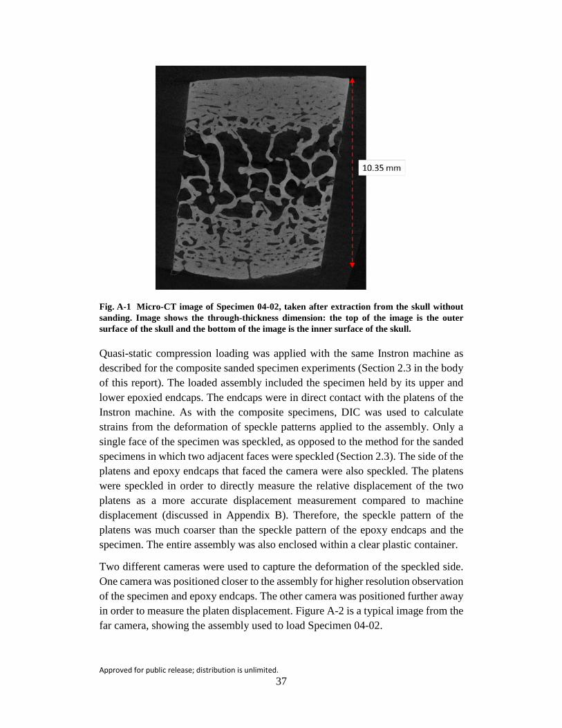
Approved for public release; distribution is unlimited. 37
Fig. A-1 Micro-CT image of Specimen 04-02, taken after extraction from the skull without sanding. Image shows the through-thickness dimension: the top of the image is the outer surface of the skull and the bottom of the image is the inner surface of the skull.
Quasi-static compression loading was applied with the same Instron machine as described for the composite sanded specimen experiments (Section 2.3 in the body of this report). The loaded assembly included the specimen held by its upper and lower epoxied endcaps. The endcaps were in direct contact with the platens of the Instron machine. As with the composite specimens, DIC was used to calculate strains from the deformation of speckle patterns applied to the assembly. Only a single face of the specimen was speckled, as opposed to the method for the sanded specimens in which two adjacent faces were speckled (Section 2.3). The side of the platens and epoxy endcaps that faced the camera were also speckled. The platens were speckled in order to directly measure the relative displacement of the two platens as a more accurate displacement measurement compared to machine displacement (discussed in Appendix B). Therefore, the speckle pattern of the platens was much coarser than the speckle pattern of the epoxy endcaps and the specimen. The entire assembly was also enclosed within a clear plastic container.
Two different cameras were used to capture the deformation of the speckled side. One camera was positioned closer to the assembly for higher resolution observation of the specimen and epoxy endcaps. The other camera was positioned further away in order to measure the platen displacement. Figure A-2 is a typical image from the far camera, showing the assembly used to load Specimen 04-02.

Approved for public release; distribution is unlimited. 38
Fig. A-2 Image from the far camera of the assembly of Specimen 04-02, prior to compression. The difference in speckle density between the platens and the assembly is clearly visible.
For Specimen 04-02, the clear plastic container was filled with Hank’s Buffered Saline Solution HBSS in order to hydrate the specimen during loading. However, the submerged specimen began to extrude air bubbles from the diploë during compression. The bubbles accumulated on the diploë face of the specimen and would also ascend the face toward the top of the specimen as the loading continued. This process obscured the speckle pattern, causing a loss of image correlation. Therefore, HBSS was not used with other specimens, as using HBSS also added additional experimental difficulties in assembling the loading components inside the Instron machine, and prevented the use of two cameras. Unfortunately, compression loading of the specimen in air (without HBSS) did not solve this problem, as HBSS fluid bubbles (originating from inside the specimen structure) still formed on the specimen surface after the yield point. This was the case for both the unsanded and sanded sandwich-structure experiments.
For specimens 04-01 and 04-03, the test was aborted soon after extruded material and bubbles started to obscure the speckled specimen face. The experiment with
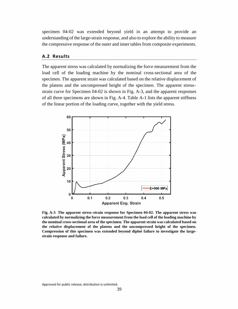
Approved for public release; distribution is unlimited. 39
specimen 04-02 was extended beyond yield in an attempt to provide an understanding of the large-strain response, and also to explore the ability to measure the compressive response of the outer and inner tables from composite experiments.
A.2 Results
The apparent stress was calculated by normalizing the force measurement from the load cell of the loading machine by the nominal cross-sectional area of the specimen. The apparent strain was calculated based on the relative displacement of the platens and the uncompressed height of the specimen. The apparent stress–strain curve for Specimen 04-02 is shown in Fig. A-3, and the apparent responses of all three specimens are shown in Fig. A-4. Table A-1 lists the apparent stiffness of the linear portion of the loading curve, together with the yield stress.
Fig. A-3 The apparent stress–strain response for Specimen 04-02. The apparent stress was calculated by normalizing the force measurement from the load cell of the loading machine by the nominal cross-sectional area of the specimen. The apparent strain was calculated based on the relative displacement of the platens and the uncompressed height of the specimen. Compression of this specimen was extended beyond diploë failure to investigate the large-strain response and failure.

Approved for public release; distribution is unlimited. 40
Fig. A-4 The apparent stress–strain response for all three unsanded (assembly) specimens. Inset figure shows detail of the elastic region, with the modulus calculated for each specimen. In the inset, the region of each response curve that was considered in calculating the stiffness (or effective modulus of the sandwich structure) is shown by bolded dotted lines.
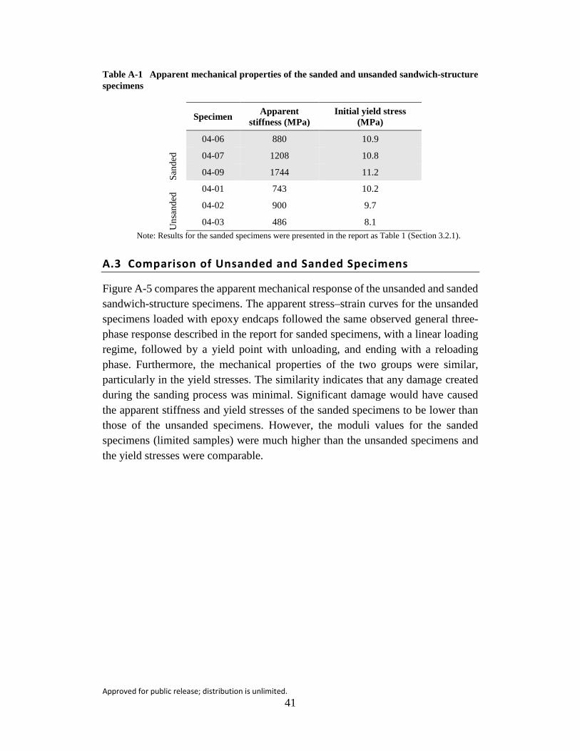
Approved for public release; distribution is unlimited. 41
Table A-1 Apparent mechanical properties of the sanded and unsanded sandwich-structure specimens
Specimen Apparent stiffness (MPa)
Initial yield stress (MPa)
Sand
ed
04-06 880 10.9
04-07 1208 10.8
04-09 1744 11.2 U
nsan
ded 04-01 743 10.2
04-02 900 9.7
04-03 486 8.1 Note: Results for the sanded specimens were presented in the report as Table 1 (Section 3.2.1).
A.3 Comparison of Unsanded and Sanded Specimens
Figure A-5 compares the apparent mechanical response of the unsanded and sanded sandwich-structure specimens. The apparent stress–strain curves for the unsanded specimens loaded with epoxy endcaps followed the same observed general three-phase response described in the report for sanded specimens, with a linear loading regime, followed by a yield point with unloading, and ending with a reloading phase. Furthermore, the mechanical properties of the two groups were similar, particularly in the yield stresses. The similarity indicates that any damage created during the sanding process was minimal. Significant damage would have caused the apparent stiffness and yield stresses of the sanded specimens to be lower than those of the unsanded specimens. However, the moduli values for the sanded specimens (limited samples) were much higher than the unsanded specimens and the yield stresses were comparable.
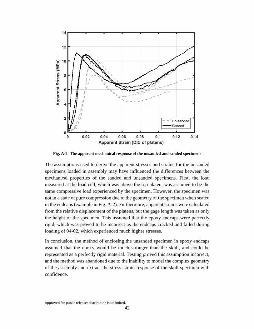
Approved for public release; distribution is unlimited. 42
Fig. A-5 The apparent mechanical response of the unsanded and sanded specimens
The assumptions used to derive the apparent stresses and strains for the unsanded specimens loaded in assembly may have influenced the differences between the mechanical properties of the sanded and unsanded specimens. First, the load measured at the load cell, which was above the top platen, was assumed to be the same compressive load experienced by the specimen. However, the specimen was not in a state of pure compression due to the geometry of the specimen when seated in the endcaps (example in Fig. A-2). Furthermore, apparent strains were calculated from the relative displacement of the platens, but the gage length was taken as only the height of the specimen. This assumed that the epoxy endcaps were perfectly rigid, which was proved to be incorrect as the endcaps cracked and failed during loading of 04-02, which experienced much higher stresses.
In conclusion, the method of enclosing the unsanded specimen in epoxy endcaps assumed that the epoxy would be much stronger than the skull, and could be represented as a perfectly rigid material. Testing proved this assumption incorrect, and the method was abandoned due to the inability to model the complex geometry of the assembly and extract the stress–strain response of the skull specimen with confidence.

Approved for public release; distribution is unlimited. 43
Appendix B. Machine Compliance in Displacement Measurements

Approved for public release; distribution is unlimited. 44
The outer and inner surfaces of the specimen were compressed by platens. Therefore, the global displacement applied to the specimen was given by the relative displacement between the two platens. Two different methods were used to measure this displacement. The first method was based on the displacement output from the Instron loading machine, hereafter referred to as the machine displacement. The second method was derived from digital image correlation (DIC) of the platens themselves, as described in Section 2.3. In this method, the platens were speckled and part of these speckle patterns was included in the field of view of the images captured during the experiment (Fig. 2 in the body of this report). VIC-2D software (Correlated Solutions) was used for DIC of these speckle patterns during loading, and the relative displacement between the two platens was obtained from this DIC analysis. This measured displacement is hereafter referred to as the platen displacement.
Figures B-1 through B-3 compare the two measures of displacement during the compression tests of Specimens 04-06, 04-07, and 04-09. The difference between the machine displacement and the platen displacement is plotted as a function of time, together with the apparent stress (load/area). The machine displacement was consistently higher than the platen displacement, and the magnitude of this overestimation generally increased with stress. This discrepancy is caused by compliance in the loading train and demonstrated why the use of highly accurate optical techniques is required, especially when measuring elastic properties, which are highly sensitive to the strain measurement.
Fig. B-1 Compliance error for Specimen 04-06
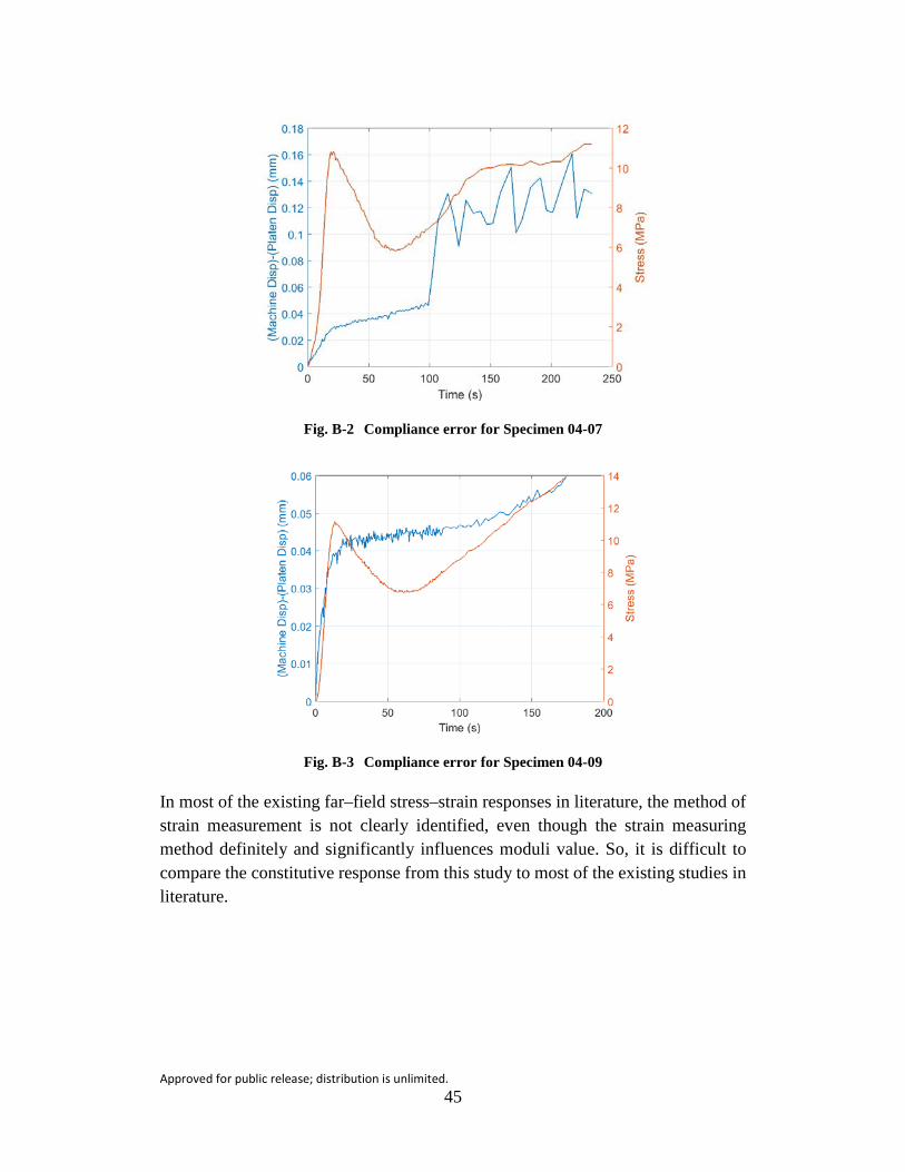
Approved for public release; distribution is unlimited. 45
Fig. B-2 Compliance error for Specimen 04-07
Fig. B-3 Compliance error for Specimen 04-09
In most of the existing far–field stress–strain responses in literature, the method of strain measurement is not clearly identified, even though the strain measuring method definitely and significantly influences moduli value. So, it is difficult to compare the constitutive response from this study to most of the existing studies in literature.
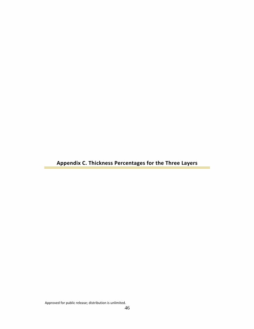
Approved for public release; distribution is unlimited. 46
Appendix C. Thickness Percentages for the Three Layers

Approved for public release; distribution is unlimited. 47
Section 3.1.2 in the body of this report referenced the method used previously1 to identify the boundaries between the three layers. For reference, Table C-1 is reproduced from the previous report, showing the average thickness percentage of each layer. These thicknesses represent the percentage of total thickness occupied by each of the three layers. The thickness percentages are reported as averages over a given extraction grid (e.g., the frontal bone of Skull 04), for each skull (Skull 04, Skull 06, and Skull 10), for each bone type (frontal and parietal), and as a grand average over all specimens. Figure C-1 plots the averages by bone type, showing the differences between the frontal and parietal bones.
Table C-1 Thickness percentage (%) of each layer (mean ± std)
Skull Section Inner table Diploe Outer table
Skull 04 Frontal 23.5 ± 5.3 53.1 ± 5.0 23.5 ± 3.2
Skull 04 Parietal 13.3 ± 3.5 68.1 ± 7.9 18.6 ± 5.3
Skull 06 Frontal 35.8 ± 12.0 42.9 ± 12.4 21.2 ± 1.6
Skull 06 Parietal 13.0 ± 2.9 71.3 ± 5.4 15.7 ± 4.2
Skull 07 Frontal 25.7 ± 8.9 52.6 ± 11.1 21.7 ± 3.0
Skull 10 Frontal 43.1 ± 8.6 33.5 ± 8.3 23.3 ± 2.6
Skull 10 Parietal 17.4 ± 6.3 58.6 ± 11.2 24.1 ± 6.4
Skull 04 (combined) 18.4 ± 6.8 60.6 ± 10.0 21.0 ± 5.0
Skull 06 (combined) 24.4 ± 14.5 57.1 ± 17.3 18.5 ± 4.2
Skull 10 (combined) 30.3 ± 15.1 46.1 ± 16.1 23.7 ± 4.8
(combined) Frontal 32.0 ± 11.8 45.5 ± 12.3 22.4 ± 2.7
(combined) Parietal 14.6 ± 4.7 66.0 ± 9.8 19.4 ± 6.3
(combined) (combined) 24.6 ± 12.8 54.3 ± 15.2 21.1 ± 4.8
1 Alexander SL, Karin R, Gunnarsson CA, Weerasooriya T. Morphological characterization of the
frontal and parietal bones of the human skull. Aberdeen Proving Ground (MD): Army Research Laboratory (US); 2017. Report No.: ARL-TR-7962.

Approved for public release; distribution is unlimited. 48
Fig. C-1 Thickness percentage of the outer table, diploë, and inner table, averaged by bone type as reported in ARL-TR-7962. Differences between frontal and parietal bone thicknesses are significant (Alexander et al. 2017).

Approved for public release; distribution is unlimited. 49
Appendix D. Moduli Values for Each Specimen
Approved for public release; distribution is unlimited. 50
Tables D-1 through D-7 show the tabulated three-layer and composite moduli for every skull specimen, as described in Section 3.5.2 (these moduli were presented as averages in Table 4 and Fig. 15 in the body of this report). All of the moduli in this appendix are in units of gigapascals (GPa).
Table D-1 Moduli for specimens from the frontal bone of Skull 04
Specimen Inner table Diploë Outer table Composite (𝑬𝑬�)
04-01 6.24 2.01 7.90 3.17
04-02 6.35 1.63 7.63 2.66
04-03 6.49 1.85 7.73 2.79
04-04 6.31 1.86 7.96 2.98
04-05 5.81 1.95 7.63 2.77
04-06 6.82 2.11 7.98 3.08
04-07 6.49 2.00 8.02 3.00
04-08 5.38 2.11 7.65 2.84
04-09 6.36 2.23 7.96 3.48
Mean±std 6.25 ± 0.42 1.97 ± 0.18 7.83 ± 0.17 2.97 ± 0.25
Table D-2 Moduli for specimens from the parietal bone of Skull 04
Specimen Inner table Diploë Outer table Composite (𝑬𝑬�)
04-10 6.31 2.02 7.46 2.49
04-11 6.94 2.10 7.33 2.89
04-12 7.08 2.15 7.54 3.06
04-13 6.51 1.68 7.15 1.95
04-14 7.39 1.89 6.98 2.48
04-15 6.63 2.04 6.55 2.74
04-16 7.01 1.84 7.01 2.19
04-17 6.80 1.70 6.66 2.28
04-18 7.12 1.78 7.16 2.43
Mean±std 6.87 ± 0.34 1.91 ± 0.18 7.09 ± 0.34 2.50 ± 0.35
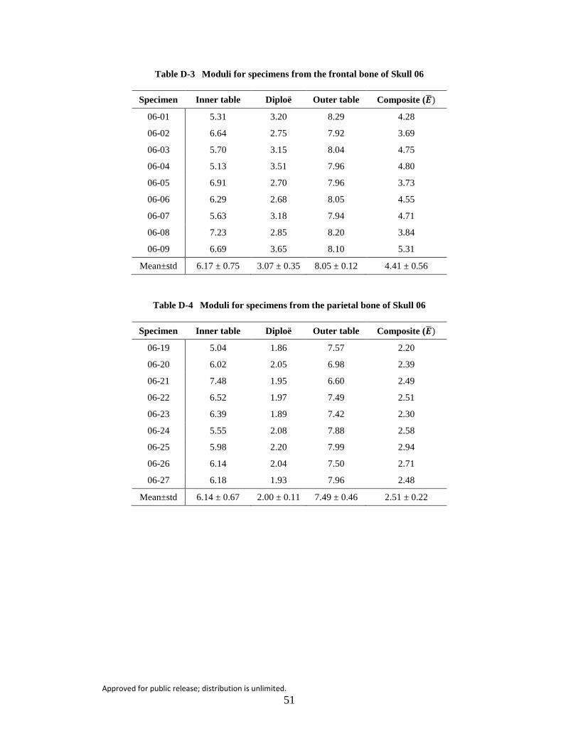
Approved for public release; distribution is unlimited. 51
Table D-3 Moduli for specimens from the frontal bone of Skull 06
Specimen Inner table Diploë Outer table Composite (𝑬𝑬�)
06-01 5.31 3.20 8.29 4.28
06-02 6.64 2.75 7.92 3.69
06-03 5.70 3.15 8.04 4.75
06-04 5.13 3.51 7.96 4.80
06-05 6.91 2.70 7.96 3.73
06-06 6.29 2.68 8.05 4.55
06-07 5.63 3.18 7.94 4.71
06-08 7.23 2.85 8.20 3.84
06-09 6.69 3.65 8.10 5.31
Mean±std 6.17 ± 0.75 3.07 ± 0.35 8.05 ± 0.12 4.41 ± 0.56
Table D-4 Moduli for specimens from the parietal bone of Skull 06
Specimen Inner table Diploë Outer table Composite (𝑬𝑬�)
06-19 5.04 1.86 7.57 2.20
06-20 6.02 2.05 6.98 2.39
06-21 7.48 1.95 6.60 2.49
06-22 6.52 1.97 7.49 2.51
06-23 6.39 1.89 7.42 2.30
06-24 5.55 2.08 7.88 2.58
06-25 5.98 2.20 7.99 2.94
06-26 6.14 2.04 7.50 2.71
06-27 6.18 1.93 7.96 2.48
Mean±std 6.14 ± 0.67 2.00 ± 0.11 7.49 ± 0.46 2.51 ± 0.22

Approved for public release; distribution is unlimited. 52
Table D-5 Moduli for specimens from the frontal bone of Skull 07
Specimen Inner table Diploë Outer table Composite (𝑬𝑬�)
07-10 6.84 3.50 7.94 4.32
07-11 6.84 3.41 8.08 4.54
07-12 7.35 3.26 8.06 4.81
07-13 7.32 3.30 7.95 4.02
07-14 6.81 2.63 8.10 3.90
07-15 7.10 3.18 8.07 4.67
07-16 6.57 3.30 7.68 4.03
07-17 6.62 2.85 8.06 4.25
07-18 6.77 3.43 8.12 5.08
Mean±std 6.91 ± 0.28 3.21 ± 0.29 8.01 ± 0.14 4.40 ± 0.40
Table D-6 Moduli for specimens from the frontal bone of Skull 10
Specimen Inner table Diploë Outer table Composite (𝑬𝑬�)
10-01 7.39 1.67 8.30 3.42
10-02 7.37 2.21 8.14 4.31
10-03 6.88 2.88 8.20 5.35
10-04 6.92 1.46 8.23 3.08
10-05 7.57 1.94 8.36 3.45
10-06 7.42 2.83 8.18 5.11
10-07 6.64 2.01 8.23 4.05
10-08 7.28 1.71 8.13 2.78
10-09 6.87 2.35 8.10 4.65
Mean±std 7.15 ± 0.32 2.12 ± 0.50 8.21 ± 0.08 4.02 ± 0.91

Approved for public release; distribution is unlimited. 53
Table D-7 Moduli for specimens from the parietal bone of Skull 10
Specimen Inner table Diploë Outer table Composite (𝑬𝑬�)
10-10 6.05 1.26 7.49 1.55
10-11 6.47 2.33 7.98 3.17
10-12 7.48 2.92 8.04 4.48
10-13 6.81 0.67 7.41 0.91
10-14 7.45 2.13 7.60 3.01
10-15 7.15 2.70 8.08 4.20
10-16 6.66 1.25 7.71 1.77
10-17 7.00 1.54 8.11 2.32
10-18 7.35 1.61 8.20 2.71
Mean±std 6.94 ± 0.48 1.82 ± 0.74 7.85 ± 0.30 2.68 ± 1.19

Approved for public release; distribution is unlimited. 54
List of Symbols, Acronyms, and Abbreviations
3-D 3-dimensional
ARL US Army Research Laboratory
BVF bone volume fraction
CSA cross-sectional area
DIC digital image correlation
FEA finite element analysis
HBSS Hank’s Buffered Saline Solution
IT inner table
MD mid-diploë
micro-CT microcomputed tomography
OT outer table
PMHS postmortem human subject
VOI volume of interest

Approved for public release; distribution is unlimited. 55
1 DEFENSE TECHNICAL (PDF) INFORMATION CTR DTIC OCA 2 DIR ARL (PDF) IMAL HRA RECORDS MGMT RDRL DCL TECH LIB 1 GOVT PRINTG OFC (PDF) A MALHOTRA 11 NATICK SOLDIER RSRCH (PDF) DEV AND ENG CTR M G CARBONI D COLANTO R DILLALLA J FONTECCHIO B KIMBALL J KIREJCZYK J PARKER M MAFEO M MARKEY D PHELPS J WARD 2 PROG EXECUTIVE OFC (PDF) SOLDIER A FOURNIER J MULLENIX 1 MTRL SCIENCES DIV (PDF) LAWRENCE BERKELY NATL LAB R RITCHIE 5 SOUTHWEST RSRCH INST (PDF) C ANDERSON JR S CHOCRON D NICOLELLA T HOLMQUIST G JOHNSON 1 INST FOR DEFNS ANLYS (PDF) Y MACHERET 4 MRMC DOD BLAST INJURY (PDF) RSRCH PROGRAM COOR OFC R GUPTA M LEGGIERI T PIEHLER R SHOGE
2 MRMC JTAPIC PRGM OFC (PDF) W LEI J USCILOWICZ 4 US ARMY AEROMEDICAL (PDF) RSRCH LAB F BROZOSKI V CHANCEY B MCENTYRE D WISE 1 TARDEC (PDF) R SCHERER 1 RDECOM HQ (PDF) AMSRD PE D RUSIN 2 EDGEWOOD CHEML AND (PDF) BIOL RSRCH DEV AND ENG CTR M HORSMON N VINCELLI 1 OSD DOT&E (PDF) J IVANCIK 5 US NAVAL RSRCH LAB (PDF) A BAGCHI A ILIOPOULOS J MICHOPOULOS K TEFERRA X TAN 3 WHITING SCHOOL OF (PDF) ENGRG JOHNS HOPKINS UNIV T D NGUYEN B NOTGHI S BAILOOR 1 COULTER DEPT OF BIOL (PDF) ENGRG GEORGIA INST OF TECHLGY S MARGULIES 1 DEPT OF ENGRG SCI AND (PDF) MECHANICS VIRGINIA POLYTECHNIC INST AND STATE UNIV R BATRA
Approved for public release; distribution is unlimited. 56
2 MASSACHUSETTS INST OF (PDF) TECHLGY INST FOR SOLDIER NANOTECHNOLOGIES R RADOVITZKY S SOCRATE 1 DEPT OF MECHL AND (PDF) NUCLEAR ENGRNG THE PENNSYLVANIA STATE UNIV R KRAFT 1 INDIAN INST OF TECH (PDF) R BHARDWAJ 1 UNIV OF VIRGINIA CTR FOR (PDF) APPLIED BIOMECHANICS ROBERT SALZAR 85 ARL (PDF) RDRL CI P PLOSTINS RDRL DP S WALSH RDRL SL P BAKER RDRL SLB G DIETRICH RDRL SLB W J GURGANUS W MERMAGEN S SNEAD RDRL WM S KARNA A RAWLETT RDRL WML W OBERLE RDRL WML F G BROWN RDRL WML H T EHLERS L MAGNESS C MEYER J NEWILL D SCHEFFLER B SCHUSTER RDRL WM S SCHOENFELD RDRL WMM J BEATTY J MCCAULEY J SINGH M VANLANDINGHAM
RDRL WMM A D O’BRIEN T PLAISTED E WETZEL C YEN K STRAWHECKER RDRL WMM B G GAZONAS D GRAY B LOVE P MOY T WALTER V WU RDRL WMM C R JENSEN RDRL WMM D A BUJANDA R CARTER B CHEESEMAN E CHIN J SIETINS J SOUTH RDRL WMM E G GILDE J LASALVIA P PATEL J SWAB L VARGAS-GONZALEZ RDRL WMM F R DOWDING S GRENDAHL RDRL WMM G J LA SCALA J LENHART K MASSER R MROZEK RDRL WMP A S BILYK RDRL WMP B S ALEXANDER A BROWN A DAGRO A DILEONARDI A EIDSMORE A GUNNARSSON C HAMPTON C HOPPEL M KLEINBERGER J MCDONALD P MCKEE K RAFAELS M SCHEIDLER K THOMPSON T WEERASOORIYA S WOZNIAK
Approved for public release; distribution is unlimited. 57
T ZHANG RDRL WMP C R BECKER J BRADLEY D CASEM C MEREDITH S SATAPATHY A SOKOLOW RDRL WMP D R DONEY B SCOTT C RANDOW RDRL WMP E M BURKINS P GILLICH M LOVE P SWOBODA RDRL WMP F N GNIAZDOWSKI R GUPTA X HUANG